International Conference on Mechanical Engineering Research (ICMER2013), 1-3 July 2013

Bukit Gambang Resort City, Kuantan, Pahang, Malaysia

Organized by Faculty of Mechanical Engineering, Universiti Malaysia Pahang

Paper ID: P132

1

SMART METHODOLOGY OF STIFFNESS NONLINEARITY

IDENTIFICATION VIBRATION SYSTEM

M.S.M. Sani 1,2

, H. Ouyang2

J.E. Cooper3 and C.K.E.Nizwan

1

1Faculty of Mechanical Engineering, University Malaysia Pahang

26600 Pekan, Pahang, Malaysia

Phone : +609-4242246 ; Fax : +609-4246325

Email: mshahrir@ump.edu.my 2Dynamics Group, School of Engineering, University of Liverpool,

Liverpool L69 3GH, UK

Email: H.Ouyang@liverpool.ac.uk 3Department of Aerospace, Faculty of Engineering, University of Bristol,

Bristol, BS8 1 TR, UK

Email: j.e.cooper@bristol.ac.uk

ABSTRACT

Nonlinear identification is a very popular topic in the area of structural dynamics.

Detection, localisation and quantification of nonlinearities are very important steps for

assessing faults or damages in engineering structures. There have been many studies of

identifying structural nonlinearities based on vibration data but most methods are only

suitable for a small number of degrees of freedom and few nonlinear terms. In this

paper, a procedure that utilises the restoring force surface method is developed in order

to identify the parameters of nonlinear properties such as cubic stiffness, bilinear

stiffness or free play. This method employs measured vibration data, and can be applied

to structures of many degrees-of-freedom. In this paper, NASTRAN is used to compute

the frequencies and modes of the structure under study. The simulated nonlinear model

is formulated in modal space with additional terms representing nonlinear behaviour.

Nonlinear curve fitting then enables interpretation of the nonlinear stiffness via the

restoring force surface. The method is shown by MATLAB simulations to yield quite

accurate identification of stiffness nonlinearity.

Keywords: Nonlinearity, structural identification, cubic stiffness, bilinear stiffness, free

play

INTRODUCTION

Linear identification methods have been widely explored by researchers over the last 35

years and are now a mature approach. Generally, most structures exhibit some degree of

nonlinearity characteristics (Dearson, 1994: Worden et al., 2001: Ewins, 1999).

Nonlinearity can present extremely complex behaviour which linear systems cannot

(Worden et al., 2001). Furthermore, nonlinear dynamic analysis becomes very important

for the identification of damage in structures. Detection, localisation and quantification

of nonlinearity are very common in nonlinear structural dynamics area (Ewins, 1999).

The identification of nonlinear dynamic systems is increasingly a necessity for

industrial applications of full-scale structures.

Initially, non-parametric identification of nonlinear system was proposed (Peng

et al., 2007) which certain constraint made on the type of nonlinear identification. This

brought to you by COREView metadata, citation and similar papers at core.ac.uk

provided by UMP Institutional Repository

2

method assumed that system mass matrix M must be diagonal, symmetric and excitation

of the force should be directly applied to discrete mass locations.

This paper presents a method or procedure for the identification of non-linear

single and multi degree-of-freedom using restoring forces method with three types of

nonlinearity. Even though the method is general, the application highlighted in this

paper suitable for non-linear identification.

RESTORING SURFACE METHOD

The equation of motion for SDOF system, can be written as

( ) ( ) (1)

where m is the mass, is the acceleration, ( ) is any applied force and ( ) is the

restoring force which is a function of velocity, and displacement, . Equation (1) can

be rewritten for the restoring force as below

( ) ( ) (2)

The restoring force surface method offers an efficient and reliable identification

of nonlinear SDOF (Platten et al., 2002). (Masri et al., 1978) described how restoring

force method could be extended to multi-degree of freedom (MDOF) systems.

Equations of motion can be transformed from physical coordinates to modal coordinates

by means of modal matrix of the linear part of the system. Velocity and displacement

can be obtained by integration of acceleration or by separate measurements and then

curve fitting to form the restoring force surface (Kerschen et al., 2003).

NONLINEAR MODAL MODEL

The equations of motion of discretised structures in the physical space can be expressed

as

( ) ( ) (3)

where M, C and K are n×n mass, damping and stiffness matrices; gnl is an n×n

nonlinear stiffness matrix, f(t)is applied nodal force vector and x(t) is the vector of

physical displacements. The equations can be obtained for example, from finite element

modelling of a structure. Transformation by leads to

( ) ( ) (4)

where is the modal vector matrix. By using orthogonality of the modes, equation (4)

become

(5)

where and are diagonal matrices, and

3

. If the structure has proportional damping, is also a

diagonal matrix and equation (5) reduces to

(6)

where is the rth modal displacement and other parameters in modal expression.

Nonlinear terms, refer to rth mode nonlinear restoring force and others mode allow

for nonlinear cross-coupling terms.

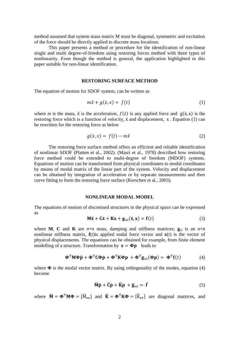
METHOD OF NONLINEAR IDENTIFICATION

Figure 1 shows the flow chart for the methodology of nonlinear identification. From

equation (6), nonlinear stiffness terms can be expressed as:

(7)

a) Choose the numbers of degree of freedom and modes to represent the system.

b) Choose a suitable input and ‘measure’ the response.

c) Assume a suitable type of nonlinearity with coefficients to be determined in step

f.

d) Set the time step, dt.

e) Compute the right-hand side of equation (7).

f) Curve fit the coefficients in step c. If the error between the two sides of equation

(7) is big, go back to step c and try with a different type of nonlinearity. If the

error is small enough, the identification is considered completed and successful.

No

Yes

Yes

No

Choose number of

modes and DOF

Suitable input and

response

Assume nonlinear

terms

Set time steps

Run simulation

Phase plot

type shape?

Plot restoring forces vs

velocity vs displacement

Curve Fitting

and Polynomial

Inverse

Analysis

Compare End

Figure 1. Methodology of Nonlinear Identification

4

NONLINEAR IDENTIFICATION FOR SDOF SYSTEM

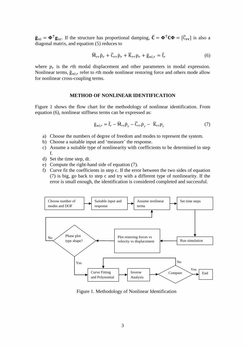
Cubic Stiffness

Consider a SDOF system with a cubic nonlinearity shown in Figure 2, with properties

as below: m=5kg, c=10 Ns/m, k=5000 N/m, gnl= 3x105 N/m

3, f(t)=100 N with chirp

signal. A chirp is a signal in which the frequency increases ('up-chirp') or decreases

('down-chirp') with time (Masri et al., 1982). Figure 3 shows the input and output of this

system. The equation of motion cubic stiffness non-linearity system is called Duffing’s

equation as follows:

( ) (8)

Figure 2. Nonlinear SDOF System

Figure 3. Input and Output of Cubic

Stiffness Nonlinearity SDOF System

Figure 4. Phase Diagram of Cubic

Stiffness Nonlinearity SDOF System

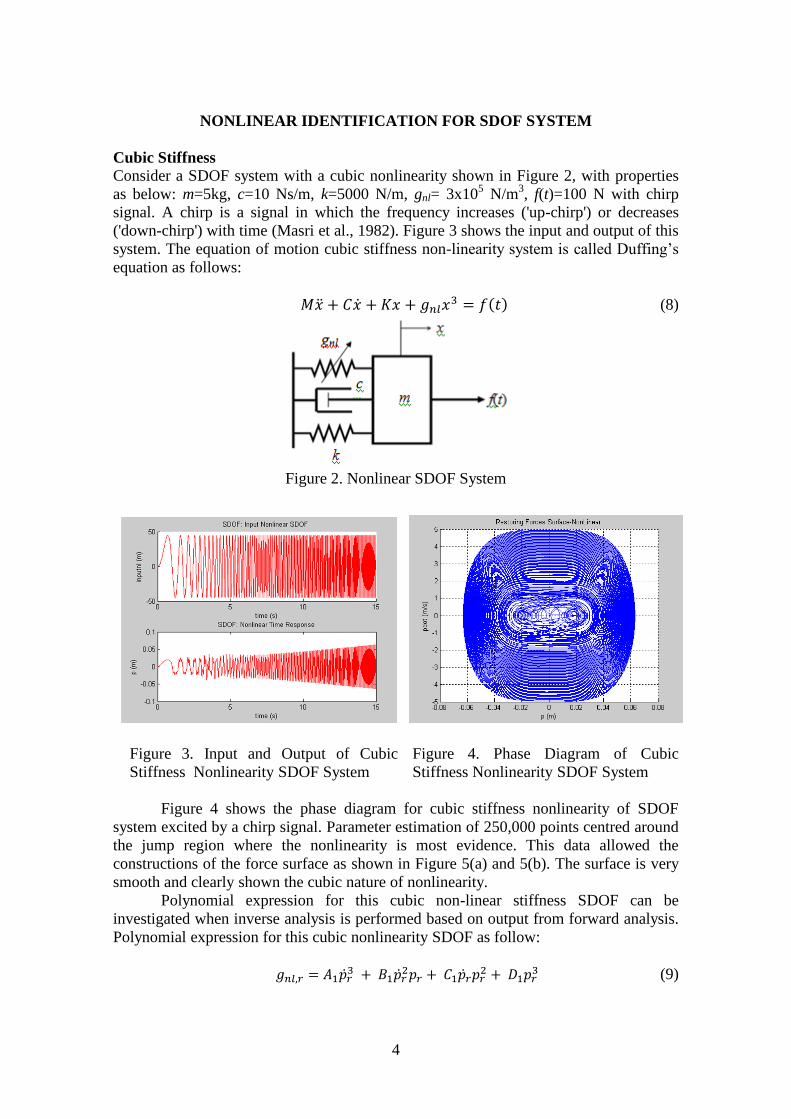
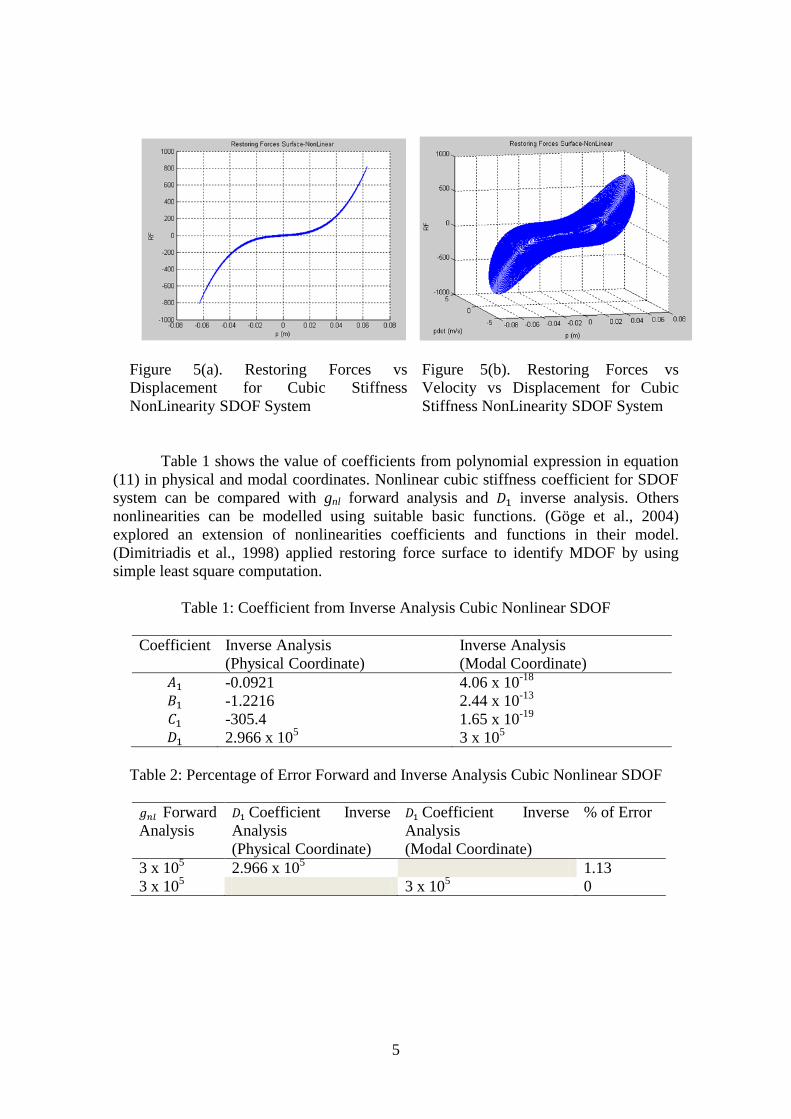
Figure 4 shows the phase diagram for cubic stiffness nonlinearity of SDOF

system excited by a chirp signal. Parameter estimation of 250,000 points centred around

the jump region where the nonlinearity is most evidence. This data allowed the

constructions of the force surface as shown in Figure 5(a) and 5(b). The surface is very

smooth and clearly shown the cubic nature of nonlinearity.

Polynomial expression for this cubic non-linear stiffness SDOF can be

investigated when inverse analysis is performed based on output from forward analysis.

Polynomial expression for this cubic nonlinearity SDOF as follow:

(9)

5

Figure 5(a). Restoring Forces vs

Displacement for Cubic Stiffness

NonLinearity SDOF System

Figure 5(b). Restoring Forces vs

Velocity vs Displacement for Cubic

Stiffness NonLinearity SDOF System

Table 1 shows the value of coefficients from polynomial expression in equation

(11) in physical and modal coordinates. Nonlinear cubic stiffness coefficient for SDOF

system can be compared with gnl forward analysis and inverse analysis. Others

nonlinearities can be modelled using suitable basic functions. (Göge et al., 2004)

explored an extension of nonlinearities coefficients and functions in their model.

(Dimitriadis et al., 1998) applied restoring force surface to identify MDOF by using

simple least square computation.

Table 1: Coefficient from Inverse Analysis Cubic Nonlinear SDOF

Coefficient Inverse Analysis

(Physical Coordinate)

Inverse Analysis

(Modal Coordinate)

-0.0921 4.06 x 10-18

-1.2216 2.44 x 10-13

-305.4 1.65 x 10-19

2.966 x 105

3 x 105

Table 2: Percentage of Error Forward and Inverse Analysis Cubic Nonlinear SDOF

Forward

Analysis

Coefficient Inverse

Analysis

(Physical Coordinate)

Coefficient Inverse

Analysis

(Modal Coordinate)

% of Error

3 x 105 2.966 x 10

5 1.13

3 x 105 3 x 10

5 0

6

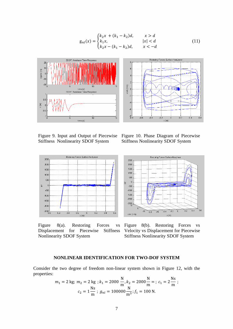
Bilinear (damping) Stiffness

Consider a SDOF system with a bilinear stiffness shown in Figure 2, with properties as

below: m=5kg, c=10 Ns/m, k1=5000 N/m, k2= 3x105 N/m, f(t)=100 N with chirp signal.

The force displacement characteristics bilinear stiffness nonlinearity system as:

( ) {

(10)

Figure 6. Input and Output of Bilinear

Stiffness Nonlinearity SDOF System

Figure 7. Phase Diagram of Bilinear

Stiffness Nonlinearity SDOF System

Figure 8(a). Restoring Forces vs

Displacement for Bilinear Stiffness

Nonlinearity SDOF System

Figure 8(b). Restoring Forces vs

Velocity vs Displacement for Bilinear

Stiffness Nonlinearity SDOF System

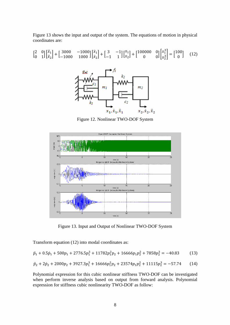
Piecewise Stiffness

Consider a SDOF system with a piecewise or backlash nonlinear stiffness shown in

Figure 2, with properties as below: m=5kg, c=10 Ns/m, k1=5000 N/m, k2= 3x105 N/m,

f(t)=100 N with chirp signal. The force displacement characteristics piecewise stiffness

nonlinearity system as:

7

( ) {

( )

| |

( ) (11)

Figure 9. Input and Output of Piecewise

Stiffness Nonlinearity SDOF System

Figure 10. Phase Diagram of Piecewise

Stiffness Nonlinearity SDOF System

Figure 8(a). Restoring Forces vs

Displacement for Piecewise Stiffness

Nonlinearity SDOF System

Figure 8(b). Restoring Forces vs

Velocity vs Displacement for Piecewise

Stiffness Nonlinearity SDOF System

NONLINEAR IDENTIFICATION FOR TWO-DOF SYSTEM

Consider the two degree of freedom non-linear system shown in Figure 12, with the

properties:

8

Figure 13 shows the input and output of the system. The equations of motion in physical

coordinates are:

[

] [

] [

] [

] [

] [

] [

] [

] [

] (12)

Figure 12. Nonlinear TWO-DOF System

Figure 13. Input and Output of Nonlinear TWO-DOF System

Transform equation (12) into modal coordinates as:

(13)

(14)

Polynomial expression for this cubic nonlinear stiffness TWO-DOF can be investigated

when perform inverse analysis based on output from forward analysis. Polynomial

expression for stiffness cubic nonlinearity TWO-DOF as follow:

9

(15)

(16)

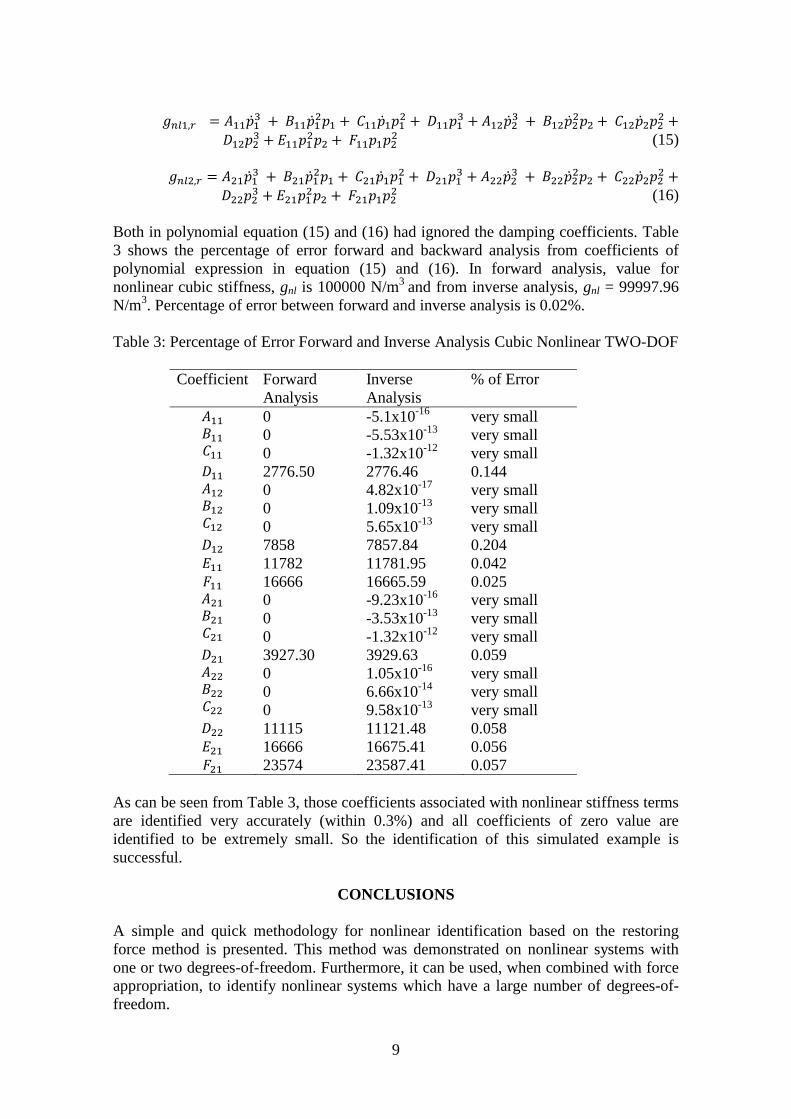
Both in polynomial equation (15) and (16) had ignored the damping coefficients. Table

3 shows the percentage of error forward and backward analysis from coefficients of

polynomial expression in equation (15) and (16). In forward analysis, value for

nonlinear cubic stiffness, gnl is 100000 N/m3

and from inverse analysis, gnl = 99997.96

N/m3. Percentage of error between forward and inverse analysis is 0.02%.

Table 3: Percentage of Error Forward and Inverse Analysis Cubic Nonlinear TWO-DOF

Coefficient Forward

Analysis

Inverse

Analysis

% of Error

0

0

0

-5.1x10-16

-5.53x10-13

-1.32x10-12

very small

very small

very small

2776.50

0

0

0

2776.46

4.82x10-17

1.09x10-13

5.65x10-13

0.144

very small

very small

very small 7858 7857.84 0.204 11782 11781.95 0.042

16666

0

0

0

16665.59

-9.23x10-16

-3.53x10-13

-1.32x10-12

0.025

very small

very small

very small

3927.30

0

0

0

3929.63

1.05x10-16

6.66x10-14

9.58x10-13

0.059

very small

very small

very small 11115 11121.48 0.058 16666 16675.41 0.056 23574 23587.41 0.057

As can be seen from Table 3, those coefficients associated with nonlinear stiffness terms

are identified very accurately (within 0.3%) and all coefficients of zero value are

identified to be extremely small. So the identification of this simulated example is

successful.

CONCLUSIONS

A simple and quick methodology for nonlinear identification based on the restoring

force method is presented. This method was demonstrated on nonlinear systems with

one or two degrees-of-freedom. Furthermore, it can be used, when combined with force

appropriation, to identify nonlinear systems which have a large number of degrees-of-

freedom.

10

ACKNOWLEDGEMENT

Mohd Shahrir Mohd Sani would like to thank the Malaysian Ministry of Higher

Education (MOHE) and the Universiti Malaysia Pahang (UMP) for their support. This

work was carried out in the Centre for Engineering Dynamics, University of Liverpool,

with the second and third authors being the PhD supervisors.

REFERENCES

Dearson, R.K. 1994. Discrete time dynamic model. Oxford University Press.

Dimitriadis,G. and Cooper, J.E. 1998. A method for identification of nonlinear multi-

degree of freedom systems. Journal of Aerospace Engineering, 212(4):287–298.

Ewins, D.J. 1999. Modal testing: Theory, practice and application. Hertfordshire

:Research Studies Press Ltd.

Göge, D., Sinapius, M., Füllekrug, U., and Link, M. 2005. Detection and description of

non-linear phenomena in experimental modal analysis via linearity plots.

International Journal of Non-Linear Mechanics, Vol. 40(1) : 27–48.

Kerschen, G. and Lenanval, J.-C. 2003. VTT Benchmark: Application of the restoring

force surface method. Mechanical Systems and Signal Processing, 17(1): 189-

193

Masri, S.F. and Caughey, T.K. 1978. A nonparametric identification technique for

nonlinear dynamics systems. Journal of Applied Mechanics, 46: 433-447

Masri, S.F., Sassi, H. and Caughey, T.K. 1982. Nonparametric identification of nearly

arbitrary nonlinear systems. Journal of Applied Mechanics, 49: 619-627.

Peng, Z.K., Lang, Z.Q., Billings, S.A and Lu, Y. 2007. Analysis of bilinear oscillators

under harmonic loading output frequency response functions. International

Journal of Mechanical Sciences, Vol. 49(11): 1213-1225.

Platten, M.F., Wright, J.R., Cooper, J.E and Sarmast, M. 2002. Identification of multi-

degree of freedom non-linear systems using and extension of force

appropriation. Proceedings of the 20th International Modal Analysis Conference,

IMAC XX, Los Angeles, USA.

Worden, K. and Tomlinson, G.R. 2001. Nonlinearity in structural dynamics: Detection,

identification and modelling. University of Sheffield: Institute of Physics

Publishing.