reliability of interconnected scheduled services

European Journal of Operational Research 79 (1994) 51-72 51 North-Holland

Theory and Methodology

Reliability of interconnected scheduled services

M a l a c h y C a r e y

Faculty of Business and Management University of Ulster, N. Ireland, UK, BT37 OQB

Received July 1992; revised December 1992

Abstract: In this paper we consider the performance of interconnected scheduled transport services for which the service times have a significant random element. That is, the arrival and departure times vary randomly from trip to trip. Any delay to a service can affect its punctuality at later stops and can affect all following services. For specificity we refer mainly to scheduled train services throughout. The reliability and performance of schedules is often investigated by stochastic simulation. However, by adopting a more analytic approach we are able to: (a) derive some properties of various measures of performance and, (b) more easily find improved or optimized schedules. Both (a) and (b) can be difficult or intractable using a simulation approach. We define various measures of reliability and performance for scheduled services, and show how to compute these. We also show how to compute or adjust schedules so as to satisfy reliability goals or targets, or optimize costs or benefits, including reliability costs. We derive various properties of these measures of reliability. In particular, we consider how reliability and costs vary in response to varying the scheduled trip times and station dwell times, or arrival and departure times. To ensure generality, we do not specify any particular forms for any of the distributions of trip times, etc. - they can be theoretical or empirical.

Keywords: Transportation; Reliability; Scheduling

I. Introduction

When designing or revising timetables or schedules for scheduled transport services (bus, train, air, etc), it is desirable to have some measures of the effects on the reliability or robustness of the timetable. For example, what effect will the changes in the schedule have on expected (mean) lateness, or on the costs or variance of lateness? What will be the probability of arriving 5, 10, etc. minutes late?

The usual way in which such measures of reliability are obtained is by simulation, using either empirical or theoretical probability distributions of trip times, station delay times, etc. However,

Correspondence to: M. Carey, Faculty of Business, University of Ulster, N. Ireland, UK, BT37 0QB.

0377-2217/94/$07.00 © 1994 - Elsevier Science B.V. All rights reserved SSDI 0377-2217(93)E0004-H

52 M. Carey / Reliability of interconnected scheduled services

simulation is often costly. More importantly, it does not easily tell us in what direction to adjust the timetable so as to improve or optimize performance. Further, it does not yield analytical insights into the measures of performance. An alternative is to take a purely analytic approach, assuming particular theoretical distributions of link trip times, etc. However, this analytical approach is tractable only for special very simple cases.

The approach adopted here is partly analytic, but to ensure tractability the computations are performed by a one pass calculation or simulation. To ensure generality we do not assume any particular functional form, so that the given distributions of trip times, etc. can be either theoretical or empirical. The latter is important, since in practice only empirical distributions may be available. We numerically calculate the probability distributions for arrival and departure times, etc., hence obtaining numerical answers to questions about performance and reliability. This numerical approach can handle cases of much greater realism and complexity than a purely analytic approach. It is faster than a simulation approach, and unlike the latter it gives 'exact' answers. It is also more amenable than simulation to optimizing timetable performance or costs, and to obtaining insights into properties of these.

For specificity, we will refer mainly to scheduled train services throughout. For example, we consider a scheduled intercity or commuter passenger train service which is common in Europe and elsewhere.

As Ceder (1986) has noted, timetable construction for scheduled services has been neglected in the literature as compared with the attention devoted to the scheduling of vehicles/stock and crews to operate an already timetabled service. (For the latter scheduling problems see Wren (1981), Rousseau (1985) and Daduna and Wren (1988)). However, over the past couple of decades some authors have investigated timetable construction and the construction of optimal timetables. In general, they have been concerned with the basic matching of supply and demand: with such issues as service frequency/ headways, stopping patterns, etc., and the effect of these on the trade off between operating cost and passenger travel time/cost and waiting time/cost.

Most of this timetable modelling assumes deterministic travel times and wait times, hence it is not directly applicable to answering questions about reliability indicated above. For a rail line, the schedule and timetable construction problem has been analysed by Vuchic and Newell (1968), Salzborn (1969), Young (1970), Amit and Goldfarb (1971), Saha (1975) and others - see the still useful surveys in Assad (1980, 1981). Salzborn (1970) and Nemhauser (1969) investigate using a mix of local and express services to reduce travel times or costs. More recently, Ceder (1986) presented several alternative methods for constructing timetables using passenger load data. Also, some authors (Kikuchi and Vuchic, 1982; Kikuchi, 1985; Ling and Taylor, 1988) investigated the relationship between the optimum number of stops and optimum headways for a transit route. Their objective is to minimize average user travel time or travel cost. However, all of the above work is deterministic. The authors do not consider the implications of the fact that point to point trip times, wait times, etc. are in general subject to random variation.

On the other hand, Powell and Sheffi (1983) introduce various forms of randomness affecting busses operating on a single route, and explore the interdependence of these. Their focus is different from the present paper, and is not on optimizing measures of cost and reliability as in Sections 4 and 5 below, nor on the properties developed in Sections 6 to 8 below. Chert and Harker (1990) consider the problem of estimating parameters of trip time and delay distributions for scheduled rail services subject to random delay. Jovanovic and Harker (1991, Appendix B.2), and Carey (1991, Section 5) in large scale mathematical programming approaches to rail timetabling, have included rough first order approximation methods for computing a measure of timetable robustness.

In view of the relative neglect of random variation in trip times, wait times, etc., reliability and punctuality issues have been neglected. For example the costs of arriving late or early have been neglected as compared to other costs. In view of this, we are concerned here with how to evaluate the reliability of proposed scheduled services. These methods can be used for: (a) computing reliability/punctuality costs of reducing trip times and wait times, or increasing the

number of trains per hour, (b) evaluating and comparing reliability of sections of proposed timetables,

M. Carey / Reliability of interconnected scheduled services 53

(c) adjusting/designing simple timetables to meet prespecified reliability or performance criteria (e.g., no more than say 10% of trains more than 5 minutes late), and

(d) optimizing scheduled arrival and departure times (timetables). In Section 2, we consider a single train traversing a stretch of rail line having stops at several stations

en route. In Section 3, we extend this to consider multiple trains traversing the same line, again having multiple stops. This introduces the knock-on effects which the delays to any trains may impose on following trains. In Section 4 we introduce costs of travel time and reliability costs, that is, expected costs of arriving or departing late or early. We formulate mathematical programs to minimize these costs, while satisfying stochastic travel time, wait time and headway constraints. In Section 5 we discuss solving the optimization problems from Section 4 and set out an algorithm for this. We are not particularly concerned here with developing fast efficient algorithms - hence we leave consideration of alternative algorithms for later research. Our concern here is to demonstrate the feasibility of the modelling approach. In Section 6 we set out other measures of performance and reliability as alternatives to the cost-based measures in Section 4. These include measures commonly used by operators, managers and planners. Such measures can be used to define timetable design criteria, and timetables satisfying these criteria can then be computed by sequential application of the formulae from Sections 2 and 3. In Sections 7 and 8 we derive and set out various properties of the measures of reliability from Sections 4 and 6. In particular, we consider how the various measures behave in response to changing the scheduled timing allowances - the scheduled trip time on each link and wait time at each stop.

2. Single train with stochastic trip times and wait times

In this section we derive the distributions of arrival and departure times, hence lateness or earliness, of a train at each successive scheduled stopping point. In particular, we see how these distributions depend on the scheduled departure times, or equivalently on how much time is allowing in the schedule for each leg of the journey. To do this we take as given the underlying distributions of trip times on each link and delays at each station. These latter distributions can be estimated from data which is routinely collected.

Consider a single train starting at station i = 1 and traversing links i = 1 . . . . , I - 1, joining stations i = 1 , . . . , I. Link i joins station i to i + 1. Let: T,.a,Ti d = The scheduled arrival and departure times respectively at station i. W~ = The minimum time which the train is required to wait at station i, to allow for boarding

alighting, etc. Note that W~ < r i d - r i a.

ta,t d = The actual arrival and departure times respectively at station i. t~ = The actual trip time (duration) from station i to i + 1.

Let the trip time t~ be a random variable with pdf fis(t). The trip t 2 time may also depend on the departure time t/a from station i. For example, if a train departs late from i one might expect it to compensate by travelling faster. To reflect this, write the conditional pdf of t~ as fis(t [ t¢). Since the trip times t~ are random variables it follows that the station arrival and departure times t a and t¢ are random variables. Denote the pdf's of these by fia(t) and fid(t). We derive these pdf's below.

2.1. Departure and arrival time distributions

The train departing from station i may depart on time or may depart late. Recall, that there is a minimum fixed wait time ~ at station i, hence to depart on time the train must arrive at i at or before time T/d - I4//. Thus the probability of departing on time is just the probability of arriving at station i at or before time T,. d - IV/. That is,

P (depa r t on time from station i) = F / a ( r / d - W / ) = fold--w/f/a(/) dt. (1)


A train departs late from station i if it arrives after time T / d - W/. In this case the train waits the minimum time W i and then departs, hence the departure distribution is the same as the arrival distribution with the origin shifted by W~. In summary, the departure time pdf at station i is

l 0 if t < T,. d, i.e. the train cannot depart before time T/°

f / d ( t ) = Fia(Ti d - W/) if t = T/d, i.e. if the train arrives before t i m e T/d - W/

it departs at time Ti d, (2)

~f/a(t - Wi) if t > Ti d.

By definition, (arrival time at station i + 1) = (departure time from i) + (travel time from i to i + 1), i.e.,

t a + l = ( t d + t s ) . (3)

The two terms on the right-hand side are random variables, with pdf's f /°(t) and f/s(tl ti °) respectively. Thus the pdf of the arrival time t a is the convolution 1 or sum of these: i+1

f /~ l ( t ) = f j f / d ( z ) f i s ( t -- ~" It d = z) dr . (4)

Equation (4) states f/a+l(t) in terms of f/d(.), and conversely (2) states rio(t) in terms of f/a(.). Hence, given either f ia(t) o r f/d(t) we can recursively compute fiR(t) and fjd(t) for all later stops j > i. To do this we of course also need the trip time pdf's f/s(.) and the parameters T/a, T/d and W/ used in (2) and (4).

If we are concerned with arrival time pdf's rather than departure time pdf's then it is convenient to use (2) to substitute for and eliminate f/d(~.) from (4), thus

f/a+l(t ) = Fia(z/d - Wi)fis(t - T~ d It/d = T/d) + f ~ / i a ( ' l " - ~ i ) f / s ( t - '7" I t~ = ~') dT, (5)

which states f/a+ 1(') in terms of f/a(.) without explicit reference to f/o(.). The first term on the right is the component of the pdf corresponding to trains departing from station i on time, at time T~ d. The second term is the component of the pdf corresponding to trains departing late from station i. (The latter term can be rewritten as f~-TPfia((t -- r) -- Wi)f/s('r It/d = (t -- z -- W,.)) d~'.)

Similarly, if we are interested only in departure time pdf's rather than arrival time pdf's we can use (4) to substitute for and eliminate f/a(.) from (2): this yields f/d(.) in terms of f /~l ( ' ) without explicit reference to f/a(.).

In the above model the scheduled arrival time T/a a t a station does not affect the actual arrival time or departure time for that station: it only affects whether the arrival is classified as late or early. In contrast, the scheduled departure time does affect the actual departure time (via equation (2)), and hence affects the arrival and departure times at later stations. This is because a train departs at its scheduled time if and only if it is ready. It follows that T/d and W~ rather than T,. a are the appropriate control variables to use when seeking to control the distribution of actual arrival and departure times. More formally:

Proposition. The pd f ' s f/+ 1 (" ) and fid("), o f ta+ 1 and ti d respectively, (a) can be stated as functions of Tj a and ~j for all j < i and (b) are independent of Tj a for all j.

Proof. (a) The only parameters on the right of (2) and (4) are T/a and W/. By recursive substitution of (4) in (2) and (2) in (4), f/a(. ) and fiR+ 1(') can be expressed in terms of functions of these parameters for all j < i. (b) The parameter T, a does not appear in (2) or (4). []

1 See for example Feller (1966) for pdf's of sums of random variables (convolutions). Also, the origin t = 0 for fis(t) is defined as the departure time of the train from station i, whereas the origins for lid(t) and fia(t) are defined as clock time, e.g., the start time of the train at the initial station i = 1.


2.2. Introducing stochastic delay times at stations

Above we assumed that the minimum time needed for train boarding, alighting, etc. at a station is a constant W~. In practice however the time taken for these activities is usually a random variable t w, with pdf f/w(t). For convenience define f/w(t) so as to include a required minimum wait time W~ at the station, i.e., f~w(t) = 0 for all t < W/. The time which the train is 'ready' to depart from station i is then t b = (t a + tw). The pdf of t b is the convolution of f/a(.) and f/w(.). Thus,

f /b( t ) = ~f /a(~ ' ) f /w(t -- ~') dr . (6)

Alternatively, if waiting time delays occur only after the scheduled arrival time T/a, then the time at which the train is 'ready' to depart from station i is t b = max(T/a, t a) + t w. In this case,

f/b(t) =Fia(T/a)fiw(t - T/a) + f~/ia(~')fiw(t --'r) d7 (7)

if t > Ti a, and fib(t) = 0 if t < T/a. More generally, if t w depends on the arrival time t a at station i we rewrite fiw(t) as fiw(t [ t/~). Even more generally, t w may depend on t a and on the scheduled times T/a and T/d, but the latter can be assumed to be already included in the parameters of fiw(t [ta). Which form of fib(t) holds is an empirical question.

Though the train is 'ready' to depart at time t b it is not permitted ('legally' ready) to depart until the scheduled departure time T/a. Hence, by analogy with (2), the pdf f/dO) of the departure time t d is

0 if t < T/d, i.e. the train cannot depart before t i m e T/d,

/Fib(T/b) if t = T/a, i.e. if the train is 'ready--to depart

fid(t) = / before time T/° it departs at time T/.o,

[fib(t) if t > T/d.

(2 ' )

3. Multiple trains/services with stochastic link trip times and wait times

In this section we extend the results of Section 2 from a single train to multiple trains. This involves introducing 'knock-on' effects, that is, if a train is delayed it may delay the following train(s). We assume that trains are not allowed to pass each other on a link, and that they are allowed to pass each other at stopping points only if this is prespecified in the schedule. Thus the order in which trains traverse each link is known in advance, and is adhered to even if some trains are running late.

Consider a sequence of trains v = 1, 2 . . . . . V, traversing link i in the order v = 1, 2 . . . . . For train v at s top/s ta t ion i, let: T~ a and T~ = The scheduled arrival and departure times respectively. Wvi ~-- The minimum required dwell time. t~i and t~i = The actual arrival and departure times respectively. tti = The actual trip time from i to i + 1. h~,v+~, ~ = The minimum headway required between the arrival times of trains v and v + 1.

Since trains cannot pass and since their trip times are random variables, train v - 1 may obstruct or delay train v. As a result, for each train v we need only consider delays to it caused by the train v - 1 immediately ahead of it, which in turn may be delayed by the train v - 2.immediately ahead of that, and SO on.

56 M. Carey / Reliability o f interconnected scheduled services

3.1. Arrival time distributions

Let ta/- denote the time at which train v would arrive at stop i (exit from link i - 1) if there were no preceding trains. The pdf fa.-(t) of t~/- is obtained by simply adding a v subscript throughout (4) of Section 2.1 above, thus

fo t t d s t d = x ) dx. (8) fa i - ( t ) = f ~ , i _ l ( X ) f v , i _ l ( - x I v , i - 1

However, train v exits at this time ta/- only if there is sufficient headway following the exit of the preceding train, i.e. if tai - > t~ 1 i + ha_ x,w Otherwise, train v is obstructed by train v - 1 ahead and exits at time tai = t a a v - - i , / "['- hv-l,vi" Thus,

tai= max{tai-, ( tav-l,i + h a - l , v i ) } •

It follows that

a t h a ~ [ t r a - [ q . ~ a - t - h ~ - ' , vl a f a ( t ) = f v - l , i ( - - v - l , v i ] J o J v i k I dT 'Jc - fv i ( t ) fo f v _ l , i ( T ) dr. (9)

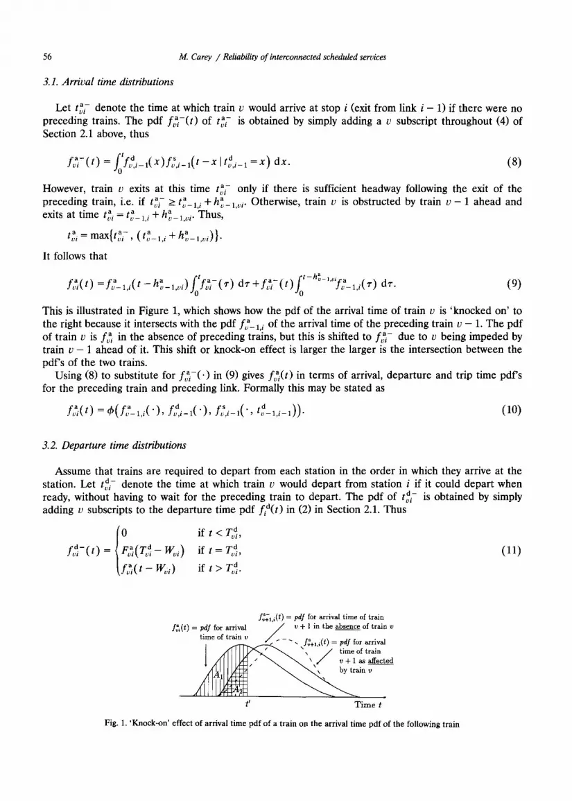
This is illustrated in Figure 1, which shows how the pdf of the arrival time of train v is 'knocked on' to the right because it intersects with the pdf f~_ 1,~ of the arrival time of the preceding train v - 1. The pdf of train v is f~. in the absence of preceding trains, but this is shifted to f ~ - due to v being impeded by train v - 1 ahead of it. This shift or knock-on effect is larger the larger is the intersection between the pdf's of the two trains.

Using (8) to substitute for f a - ( . ) in (9) gives fai(t) in terms of arrival, departure and trip time pdf's for the preceding train and preceding link. Formally this may be stated as

f~.(t) = ~ b ( f a _ l , i ( " ) , d s d f v ~ , i - l ( ' ) , f ~ , i - l ( ' , t v - l , i - 1 ) ) . ( 1 0 )

3.2. Departure time distributions

Assume that trains are required to depart from each station in the order in which they arrive at the station. Let tvd. - denote the time at which train v would depart from station i if it could depart when ready, without having to wait for the preceding train to depart. The pdf of tdi - is obtained by simply adding v subscripts to the departure time pdf lid(t) in (2) in Section 2.1. Thus

0 if t < Tf ,

f d - ( t ) = F~(T~id _ Wvi) if t = Tf, (11)

~fai(t -- Wvi ) if t > T d.

f,~+x,i(t) = pdf for arrival time of train f~( t ) = pdf for arrival / v + 1 in the absenc.._____~ee of train v

time of train v , / . _ " - " - " " f,~+l i( t ) = pdf for arrival

] ~ ~ " ~ "x J time of train I d l l l l ~ , " ~ ~ ' , / v+lasaffected

•KIII ~ ~ " ~ ' \ by train v

.

t ~ T ime t

Fig. 1. 'Knock-on' effect of arrival time pdf of a train on the arrival time pdf of the following train


However, train v can depart at this time tffi- only if it is not held up by train v - 1 ahead of it. Let h~_ ~,,~ be the minimum headway required between the departure times of trains v - 1 and v. Thus train v departs at time t~- or time t ff_l,i + d h~_L~, i whichever is the later. That is,

d - max{t~i- ' t d d ( ,~- +hv_l.vi)}, tvi -- 1,i

which implies

t d = f g _ l , i ( t - d ' d - - h , lL, hv_l,vi)fof~i (7")dT-wf~i ( t ) fo f~_ l , i ( ' r ) dT-. (12)

This equation is the same as (8) but with the 'a' superscript replaced by 'd' throughout. Using (11) to substitute for f d - ( t ) in (12) gives f~,~(') in terms of fL°_l.i('), and f a(.). Formally,

f~ ( t ) = O( d fr- l , i (") , f a ( . ) ) . (13)

Using (10) to substitute in (12) for fai(') gives fd(t) in terms of arrival, departure and trip time pdf's for the preceding train and the preceding stop. It follows immediately from (10) and (13), or equivalently (8)-(9), (11)-(12), that the arrival and departure time pdf's fa(t) and fd(t) can be computed succes- sively for each train and each station, by recursive substitution, starting say from initial known departure times for each train v from some initial station. From example: (a) use (8) to compute the arrival time pdfs fa - ( t ) for each train v = 1, 2 . . . . . at stop i ignoring arrival

time 'knock-on' effects; (b) use (9) to adjust these for 'knock-on' effects, hence obtaining arrival time pdf's f,](t), for each train

v = l , 2 . . . . ; (c) use (11) to compute the departure time pdf's f~ - ( t ) ignoring departure time knock-on effects; (d) use (12) to adjust the latter for these knock-on effects, hence obtaining departure time pdfs f~(t).

Now move to s ta t ion /s top i + 1 and repeat the process (a)-(d), and so on. Alternatively, instead of dealing with all trains v = 1, 2 . . . . , for one station or stop at a time, we can deal with one train at a time for all stations i = 1, 2 . . . . . Thus, for train v, compute f~a-(t), f,a(t), f,~-(t) and f,~.(t), as in (a)-(d) above.

4. Minimizing expected costs of travel and deviation from schedule

The costs associated with travel can be stated as the sum of (a') the (expected) cost of travel time on links and wait time at stat ions/stops; (b) the (expected) cost of arriving later or earlier than scheduled at a stop; (c) the (expected) cost of departing later than scheduled from a stop. (We assume that trains are not

allowed to depart earlier than scheduled.) The stochastic component of (a') can instead be included in (b) and (c) so that (a') becomes (a) the cost of scheduled travel time on links and scheduled wait time at stations.

4.1. A single train case

Costs of scheduled travel time Let c~ be the net cost or benefit per unit (minute) of scheduled trip time on link i, so that the cost of

scheduled time on link i is (T~_ 1 - T,d)c~ • Similarly, let c w be the cost per unit of scheduled wait time at stop i, so that the cost of scheduled wait time at stop i is (Ti d - T/a)c w. The total cost of scheduled trip time plus wait time is thus

Z (T/~_l - T/d)c s -'t- (Ti d - T/a)c w. (14)


Expected costs of arriving late Late arrival means later than the scheduled arrival time T/a. However, simply summing lateness over

all stations is not very meaningful: it may involve a substantial amount of double counting of lateness. For passengers, lateness usually matters only at stations at which they board or alight, hence depends on the number and type of passengers, etc. Also, the operating cost which lateness imposes on operators can differ at each station and for each train.

Let caL(l a) denote the total cost incurred by customers a n d / o r operators if the train arrives l a minutes late at station i. For example, if the cost per minute is a constant c aL then total cost is caLl a. For passengers, c aL might be taken as proportional to the average number of passengers alighting, or their average total fare. The expected cost of late arrivals at station i is thus

E[C?L(/a)] = f(caL(t_ T/a)fia(t) dt.

The total cost of late arrivals, over all stations, is c a z aE a = ~'i= lCi (li), hence the expected total cost of late arrivals is

E[c aL] = E l t,~. caL(la)] ~ t~. E[caL(la)] = t~ " fTt:CaL(t - Tia)fia(t)dt. ( 1 5 )

Expected costs of arriving early The expected cost of arriving earlier than scheduled at a stop is closely analogous to the cost of

arriving late at a stop. Let caE(e a) denote the cost incurred by customers a n d / o r operators if the train arrives e a = T/a - t i minutes early at stop i. Then, by analogy with (15) the expected total cost due to arriving earlier than scheduled is

E[caE]=E[~i caE(ea)]= ~i E[caE(ea)] = ~i foTi'caE(zia--t)fia(t)dt. (16)

Expected cost of arriving later or earlier than scheduled The costs associated with arriving late or early can easily be combined by adding (15) and (16). Thus,

E[ca] = E[ ~i ca( Tia)] = Ei ~°~ca( Tia)fia(t) dt (17)

where ca(t - T/a) is the cost of arriving at stop i at time t. If t = T~ a the cost is ca(0) = 0.

Expected costs of departing late (later than scheduled) Let I d = t - T/d denote the lateness of departure train, relative to its scheduled departure time T~ d

from stop i. Then the expected costs due to late departure of the train from all stops i = 1 . . . . . I, is

E [ c/d] = E[ ~. c/d(l/d)] = ~_~E[c~(l~)]=i ~'~i "T,f~c~(t-- Tid)fid(t)dt. (18)

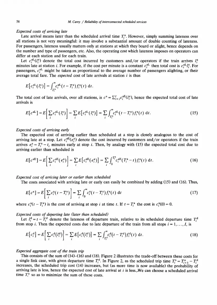
Expected aggregate cost of the train trip This consists of the sum of (14)-(16) and (18). Figure 2 illustrates the trade-off between these costs for

a single link case, with given departure time T, d. In Figure 2, as the scheduled trip time T, s= 77ai+1 - T/d increases, the scheduled trip cost (14) increases, but (as more time is now available) the probability of arriving late is less, hence the expected cost of late arrival at i is less.AVe can choose a scheduled arrival time T, a so as to minimize the sum of these costs.

M. Carey / Reliability of interconnected scheduled services

Expected lExpected ~ cost~ total costs " ' ~ - ~ J ' y - " " ~ o s t of scheduled

~ trip time, c~iT~ ', Expected costs

~ - ~ - ~ q f l a t e arrival

Minimum Optxmum Scheduled trip trip time trip time time, T~

Fig. 2. Expected trip costs vary with the scheduled arrival time Ti a

59

More generally, to minimize the expected total cost we wish to choose appropriate scheduled arrival times T~ a, i = 1 . . . . . I, and departure times T,. d, i = 1 , . . . , I. The trip cost minimizing problem for a single train v can be stated as

(P,)

Min (14) + (15) + (16) + (18), (19a) {T,a,Tf}

subject to (2 ' ) and (4) for i = 1 , . . . , I . (19b)

Equations (4) and (2) or (2') are needed since the pdf's fia(t), i = 1 . . . . . I, in (15)-(18) are interdepen- dent: f ia( t )depends on f iL l ( t )which depends on fia_z(t), and so on.

4.2. Multiple trains

To extend the above discussion (Section 4.1) to multiple trains, simply replace the i subscript with vi throughout and replace Y'-i with Y:vEi throughout. Then (14)-(18) become

E E (Ttai+l- Tf)c~,i- t - (Tt d - T ta ) c~ , (14') c' i

oo ~ l~. f a aL e [c aL] = ac2~( t - r~)fL, ~ ( t ) dt, (15')

) • T~i

T a E[caE] : c~ /~. /" "i aEz JO cvi t t -- T~a)f~'E(t) dt , (16')

oo E[ ca ] = • E f c : i ( t - T:a)f~ai(t) d t , (17')

v , i 0

f°~cdC ( t a a E[cdL] = ~ E,T,g v,, - r/ ,)C,(/) dt. (18')

The problem of minimizing travel costs for trains v = 1 . . . . , V, can then be stated as

(e)

Min (14') + (15') + (16') + (18') (20)

where the pdf's in (15')-(18') are related by (8)-(9) and (11)-(12). It is instructive to consider what happens to the solutions of programs Pv and P if we omit some of

the cost terms (14)-(18) or (14')-(18').


Example 1. Suppose that in program P~, or P we omit the costs of departing late from a station, or arriving early at the next station. In this case, there is no incentive to hold the train at stop i longer than the absolute minimum required time W//. Holding a train longer would increase the scheduled trip time without reducing the expected costs of lateness or earliness. Thus in solutions of P~ and P we have T/d - T/a = W// and T~,a/- T a = Wci r e s p e c t i v e l y .

Example 2. Suppose that in programs P~ and P we omit costs of arriving late at a stop. In this case there is no incentive to allow extra or slack trip time to reduce lateness. In an optimal solution of program P~ and P the scheduled trip time T, w will be the minimum feasible, i.e. T/w = min{t I f/w(t) > 0}.

Example 3. Suppose that in program Pv and P we omit the costs of scheduled wait time at stops. In this case in the solution of programs Pv and P the wait time W~ will be made sufficiently long as to ensure that trains always depart on time from each stop.

The discussion and propositions in Section 7 and 8 below indicate that the above problem P can be assumed to be a well-behaved optimization problem. Hence algorithms can be devised to solve it, and can be assumed to converge to a global optimum.

5. Solving problems Pv and P

In programs P~ and P as stated above the variables are the scheduled arrival and departure times To a and T d, i = 1 . . . . . I. However, it is also useful for computational and other reasons to restate programs P~, and P in terms of activity variables, scheduled trip times on links and dwell times at stations. For train v, T~ = T~ a -Td i_ l denotes the scheduled trip time on link i - 1 , and T w = T ~ - T a denotes the scheduled dwell time at stop i. Then,

i - 1 i

T a = ~] (T~) ~ + T~) and T~= E (T~) ~ + TS, y-1) • j = l j = l

Using these equations substitute for T a and T d throughout programs P~. and P. The resulting versions of programs Po and P can be referred to as Pv(T]i, Tv w) and P(T]i, TOW), to distinguish them from the previous versions P~(T a, T d) and P(T a, T~).

The effect of stating programs P~ and P in terms of scheduled trip time and dwell time variables rather than arrival and departure times (Ta, T d) can be illustrated as follows. If in program Po(T/s, T/w) we increase (decrease) some scheduled trip time T/s or dwell time T/w, holding all other (Tj s, Tj w, j ¢ i) fixed, this automatically increases (decreases) the arrival and departure times (Tfl, Tfl) at all later stops j > i. In contrast, if in program P~(T/a, T/d) we increase say T/o this increases T/w and decreases T/s leaving all other times fixed: similarly, increasing T/a increases only T/S1 and decreases only T/w.

A cyclic coordinate or recursive algorithm The following algorithms can be applied to either of the two formulations of program Po and P set

out above. However, for simplicity we will refer to only one version, namely Po(T/a, Tfl). By recursive substitution the equality constraints (2') and (4) in problem Po can be reduced to stating

fia(t) and lid(t) as functions of the given pdf's fiw,(.) and fi~,(.), and (T/a, T/,~), i ' = 1 . . . . . i. Substituting these for fia(t) and f/dO) in the cost function of problem P eliminates the fia(.) and lid(') terms, hence reduces P to an unconstrained optimization problem pV. To solve ptJ we can use any of several algorithms for optimizing functions of several variables without using derivatives. Well known methods include the cyclic coordinate method, the method of Hooke and Jeeves, the method of Rosenbrock, and variants of these methods (e.g., see Bazaraa and Shetty, 1979).


The cyclic coordinate method is not in general very efficient. However, the strongly sequential nature of the computations in program P~ suggests that a variant of the cyclic coordinate method may be useful in the present context. This can be stated as follows.

Algorithm A1 Step 1. Initialization. Set station i = 1 and set the major iteration counter k = 1. Choose a tolerance

value e for termination in Step 4, and set z 0 = + ~. Find an initial solution for problem P, (see below). Let this be (T/ag, T/dk, i = 1 . . . . . I).

Step 2. Let T/d vary. In program Pv hold all T 9, j ~ i, and all T~ a's fixed at their current values. In (2 ') and (4) in P,., T~ d affects only equations j = i . . . . . I, hence program P, reduces to

(P~,~) i

Min E ((14) + (15) + (16) + (18)) T/d j = 1

subject to (2 ' ) and (4) for j = i . . . . . I.

Program P,:rf is a function of a single variable T/d and can be solved using any of several line search algorithms (see Bazaraa and Shetty, 1979).

Step 3. Let Ti a vary. In program PL, hold all TjO's and Tj~'s fixed at their current values except for T~ a. This makes the constraints (2') and (4) in P, redundant, since T/~ does not enter into (2') or (4). Hence P,, reduces to

(P, ra) o o

Mint? (Tid--T/a)cw+fTiaCa(t--Tia)fia(t) d t + " ' ' .

Program PL, r? is a function of a single variable T/a hence can be solved using any of several line search algorithms.

Step 4. Termination. If i < I set i = i + 1 and return to Step 2. If i = I set z ~ = (the current value of the cost function in P). If z k-1 - z ~ < e then stop, and take the current solution (T/d, T/a, i = 1 . . . . , I ) as the solution of P. Otherwise, set i = 1, k -- k + 1, and return to Step 2.

Starting solutions. It is easy to obtain an initial feasible solution (T/a, T/d, i = 1 . . . . . I ) for problems PL. and P, by various methods.

Method 1. A simple starting solution is obtained by setting (Ti a, T/d) to their minimum values. The latter are obtained by setting all link trip times t~ and station dwell times t w to their minimum values. Thus,

min(t~) = min{ t l f i s ( t ) > 0} and min( t w) = IVi or min{ t l f iw( t ) > 0}.

Hence,

min(T/d) = min(T/a) + min( t~) and min(T/+l) -- min(T/d) + min(t~).

Method 2. If the optimal link trip times and station dwell times are likely to significantly or substantially exceed their minimum values then method 1 may not provide a good starting solution. In this case an alternative initial solution can be obtained as follows. Decompose program P~ or P into I separate cost minimizing programs. I_~t each program consist of optimizing with respect to (T/d_ 1, T/a) for a single link and station. Take the optimal solution of each of these simple separate problems as the starting solution for problem P,.. Similarly for program P.


6. Other measures of performance and reliability

In Section 4 we used probability distributions of train trip times to obtain expected costs of train trips. In Sections 4 and 5 we discussed minimizing the sum of these system costs. However, a common goal in service planning is often satisfying rather than optimizing: that is, satisfy certain pre-specified measures of reliability or performance. For trains, these measures or targets may differ between train types, terminal stations, intermediate stations, etc. Such measures can be used to evaluate proposed or planned train schedules, or proposed alterations or adjustments to existing schedules. Thus performance measures may be valuable at the train service planning stage as well as at the shorter run rescheduling or control stage. In the latter case, operators have to choose between a number of competing options for responding to failures, delays, etc. which cause deviations from the pre-planned schedule.

The following are some measures of train running reliability or performance which can be calculated using the pdf's of train arrival times, departure times, etc. obtained in Sections 2 and 3. 1. The probability of arriving at a station later than scheduled, or more than say k minutes later than

scheduled. A commonly used measure of service performance or reliability, for scheduled transport services, is the fraction p, or percentage 100p%, of services arriving (or departing) late or more than say 5, 10, etc. minutes late. For example, transport operators often set performance targets such as: at least 90% of services should arrive on time and say 95% should arrive no more than 10 minutes late. Also, operators, including airlines and railways, are often required to publish data on the extent to which they achieve these targets.

The probability of arriving late (i.e. after time T/a) is f~afia('r) dr, and the probability of arriving more than k minutes late is

p a ( k ) = f ~ a + / i a ( ' / " ) d ~ - = ( 1 - f i a (T / a "t - k ) ) . ( 2 1 )

Note that decreasing T/a increases pa, since from (21), (dpa/dT/a) = - f ia(Ti ~ + k ) < 0. Hence the earliest scheduled arrival time Ti a which will satisfy the reliability target p~ < ~ is the T~ ~ which yields pa =j3a

I I " By inverting F,a(") we obtain T/a as a function of pa, and hence can compute the (earliest) T/~ which

_a < /~a satisfies Pi - - i" If the density function fia(") is empirical, so that the functional form of F/a(') is not _a ffa known, it is still straightforward to find the value of T/a which yields Pi = i" Use (21), or a

summation rather than integral, to compute Zi a for given pa's and hence find the value of T/a which yields pa =~a l I "

2. The probability of departing from a station late, or more than say k minutes later than scheduled. Surveys of consumer attitudes have found that they perceive departing late as having a substantial cost or disutility, even if the serve arrives at its next destination on time. Also, departing late can have substantial costs on the operators of a service.

3. The expected (mean) lateness of arrivals or departures from a station. Expected lateness of arrivals = (expected arrival t i m e ) - (scheduled arrival time).

4. The expected costs of departing or arriving later or earlier than scheduled. These costs have already been discussed in Section 4.

5. The variance of (a) the lateness of arrivals, or (b) the earliness of arrivals, or (c) the arrival times (both late and early), or (d) the lateness of departures, at each station stop. For example, let I a = t a - Z i a

denote the lateness of arrivals at station i. Then,

var[l a] = f ((ti" - T/a) - E [ t a - T/a] )2f /a( /a) d t a = f f ( t a - Tia- E[t~] + Tia)2fia(t a) d t a • - 1 i ~

= f;~a ( t/~ -- E[ t/~]) 2 fia( t a) d t a.


Similarly, let e a = T/a - ti ~ denote earliness of arrival at station i. Then,

var[e a ] = f0~a(t? -- E [ t?] )2La ( t a) dt a.

Hence,

var[t a] = var[/a] + var[ea] .

The variance of arrival or departure times may be a more useful measure of reliability than mean lateness or earliness. For example, suppose that the mean deviation from the scheduled arrival time is say 10 minutes but the variance of the arrival time is very small. In this case the perception of lateness can be largely eliminated by simply shifting the scheduled arrival time forward 10 minutes. In contrast, suppose that the mean arrival time is close to the scheduled time but the variance is large. In this case there may be no easy way to improve the problem of perceived lateness. One of the more important potential uses of measures of performance such as 1-5 above is as design

criteria when generating train schedules. This is a valuable alternative to the 'expected cost minimizing' approach of Section 5 above. For example, suppose that the timetable design criterion is 'for each train at each station ensure that the probability of arriving, and departing, no more than 5 minutes late is 0.95'. A timetable satisfying this criterion can be calculated in one pass by starting with the first train at the first stop and proceeding sequentially from stop to stop and train to train. For each train at each stop calculate the earliest arrival and departure time which will ensure that the desired percentage of trains (say 95%) will arrive no more than 5 minutes late.

7. Properties of travel cost, performance and reliability measures as functions of scheduled trip times and dwell times

Measures of travel cost are set out in Section 4, and other measures of reliability in Section 6. Here we consider some properties of these measures. These properties provide insight into the behaviour and usefulness of the measures of reliability. They are also directly useful when computing or adjusting train schedules to improve system performance or to meet specified reliability or performance targets.

We consider how lateness at stops varies with variation in scheduled dwell times at earlier stops and scheduled trip times on earlier links. In particular, we consider how these affect (a) the probability of being late, (b) expected (average) lateness and (c) the expected costs of lateness. An important difference between the discussion in this section and the next section is as follows. Here we treat the probability of lateness, expected lateness, costs of lateness, etc., as functions of Ti~'s and TiW's, as in program P(Ti s, T~ w) in Section 5. Hence, when taking derivatives with respect to Ti w or T~ s we let all other scheduled dwell times and trip times be held ffvced. This implies that if T~ w is increased by say At, then the scheduled departure times Tj d and arrival times Tj+ 1 a t all later stops j _> i must increase by the same amount At. Similarly, it implies that if T~ ~ increases by At this increases Tj a and Tj a, for all j > i, by the same amount.

It can be shown that, under very mild conditions, cost and reliability measures have the properties set out below. Since the proofs are somewhat tedious and the results are in many cases intuitive, we will not set out full proofs in all cases.

Let E[c~(1)] denote the expected cost incurred due to arriving late at station i.

Proposition. (i) (aE[c~(l)]/aTj w) <_ 0 for all j < i

(i) This is proven in Proposition 4(i) below for the case of j = i - 1. For j < i - 2 a full proof is similar, but tedious, hence we only outline a proof here.


P r o o f (outline). An increase dTj w in Tj w allows more dwell time at stop j, hence reduces the probability of departing late from stop j. This in turn reduces the probability of arriving late at stop j + 1, since the scheduled trip time from j to j + 1 is held fixed. Further, it reduces the probability of departing late from stop j + 1, since the dwell time at j + 1 is fixed. And so on. Thus the probability of arriving and departing late at all future stops i > j tends to decrease, or at least not increase. A decrease in the probability of arriving late at a stop decreases the expected cost incurred by arriving late at the stop. []

(ii) (OE[ca(I)]/OTT) = O, for ally > i.

This holds since dwell times Tj w at stops j do not affect arrival times at earlier stops i < y.

(iii) (aE[ca(l)]/aTj s) <_ O, for ally < i.

This is proven in Proposition 5 below for the case of j = i - 1. For the case of j _< i - 2 an outline proof is similar to that given for (i) above.

(iv) (OE[ca(l)]/aTy s) = O, for ally > i.

This holds since trip times Tj s on links j > i do not affect arrival times at earlier stops i _< j.

Let E[ l a] denote expected lateness o f arrival at stop i. The same results (i)-(iv) hold as for E[ ca( la)] above. To see this, let c~(l) = l~. Then E[l a] is simply a special case o f E[ca(la)] obtained by setting, ca(l a) = 1~. Let Pia(1) denote the probability o f arriving I or more minutes late at station i. Then (v)-(x) follows.

(v) (oPia(l)/aTj ~) < O, for ally < i.

This is proven in Proposition 1 below for the case of y = i - 1. For j _< i - 2 an outline proof is similar to that given for (i) above.

(vi) (aPia(l)/aTj s) = o, for all j > i.

This holds since, in the present model, the trip time on link y does not affect the arrival times at that or earlier stations i _<y.

(vii) (aPia(l)/aTj w) < O, for ally < i.

This is proven in Proposition 2 for the case of j = i - 1. For y _< i - 2, an outline proof is similar to that given for (i) above.

(viii) (oPia(l) /aT 7 ) = O, for all y > i.

This holds since the dwell time at station j does not affect the arrival t ime at that or earlier stops i <y.

(ix) (a2Pia(l)/(OTjW) 2) >_ O, for ally < i, so that Pia(l, 7 7 ) /S convex in Tj w.

This is proven in Proposition 3(i) below for the case of j = i - 1.

(X) (O2Pia(l)/(OTjW) 2) = O, for j > i.

This holds for the same reason as (viii). We can obtain similar results for trip times Tj s as obtained for dwell times Tj w in (ix)-(x).


The above results (i)-(x) refer to late arrivals at a station. We can derive analogous results for late departures from a station. We chose to focus on late arrivals since the costs incurred due to arriving say l minutes late are usually higher than the costs incurred by departing l minutes late. The latter is in turn usually higher than the cost incurred by arriving l minutes early.

In the rest of this section we prove the results (i), (iii), (v), (vii) and (ix) above. Recall that i f ( t ) is the pdf of t a, the arrival time at stop i. The probability of arriving late (i.e., later than the scheduled arrival time Ti a) at stop i is therefore f~iafia(t) dt. More generally, the probability of arriving k or more minutes late at stop i is

oo

P/a (k) : Pi t a >_ (Ti a -~- k ) ] fTa+kfia(t) dt.

This probability of late arrival can be reduced by increasing the scheduled trip time from the previous stop, or equivalently increasing the scheduled arrival time at stop i. Thus:

Proposition 1. (oPia(k)/OTiSl) = -f ia(T/a q- k ) _~< 0.

Proof. By definition, T~ a = Tdi-1 -b T si_l, hence

Pia(k)= fT, +TiLl+/ia(t) dt'

hence

aTL1 f ia(~/dlq-Tsi -1 -l-k)= -fia( Tia-l- k ),

since (0fia(')//0T/S_ 1 = 0. But fia(Tia + k) >_ 0 since it is a pdf, hence the proposition follows. []

The following proposition shows that the probability of late arrival at stop i can be reduced by increasing the dwell time at the previous stop i - 1. The proof is much less simple than for the previous proposition, since varying T~ w_ 1 affects fia( • ) whereas varying T~ ~_ 1 does not. To simplify the proof we use the following lemma.

Lemma 1. Let f l (x [ x < O) = O. Then, fff+fttfz(~')fl(t - ~') dr dt reduces to A = ft%f2(¢)[1 - Fl(t + - z)l dt, where Fl(t +- r) = fd+ f l(t - r) dt.

Proof. Replace the integral f/- with f~-- f~. Hence,

oo c o oo oo

A = ftt ÷ f - f 2 ( ' Q f ' ( t - ' r ) d'r d t - f . ft f 2 ( ' r ) f l ( t - r ) d'; dt.

In the second integral term, the range of integration for ~" is oo > r >__ t, hence t - r < 0. But, by assumption, f l (x [ x < 0) = 0, hence f l( t - ~') = 0 over the range of integration. This reduces the second integral term above to zero, hence reduces A to A = fS+ftf2(r)fl(t - r) dr dt. The range of integration in the inner integral is now independent of the outer integral hence the order of integration can be reversed. Thus


Proposition 2. (oPia(k)/OTi w _ 1 ) __< 0. Further,

~)e/a(k) oo ---- - - f , j f/a_l('/'--W/_l)f/S_x(T/a + k - 7) d r

0T/w- 1 r, ,

= -[probabil ity of depart ing late (later than T/~_,) from stop i - 1

and arriving exactly k minutes late at stop i ] .

(22)

Remark. Recall that as explained above, f ia( t ) depends on the scheduled dwell time Tj w at previous stops j < i, and on the scheduled trip time on links j < i.

Proof. The arrival time t a at stop i is the departure time from i - 1 plus the trip time from i - 1 to i, i.e., ta = t/d- 1 + t~_ 1" The pdf of t/~ is the sum or convolution of the pdf's of ti o_ 1 and t,_l.~ The former is given

¢s its ~ hence t h e p d f o f t d i s by (2) and the latter by J i - l , i - v ,

f ia ( t a) = ' a l ( 7 - W i _ l ) f i S l ( t a - y ) dq-q-F a [ T d - W . . ~,cs ( ta_T/d_l) . (23) ._ i- l l , i -1 i - l J d i - D , i

The probability considered in the proposition is P/a(k) = f~,+~f/a(t) dt, hence from (23),

P?(k)= f , fo f / a _ l ( ' l " - W i _ l ) f i S a ( t - ' g ) d'r dt +F/a-l(Tid--l- W/-l)JT~a+k f / - l ( t - T /d l ) dt" T~ +k T,_ 1

(24)

For any scheduled service we can assume that the probability of the trip time being < 0 is zero, i.e., f/~_ t(t It < 0) = 0. This satisfies the assumption of Lemma 1. Applying Lemma 1 to the first of the two terms on the right-hand side of (24) reduces (24) to

eia(k) = f ~ d f i a l ( ~ ' - W i ' i - - 1)[1 -F'St- 1( Tia + k - ~')] d'r + Fai-ll, [T'di-1 - W / - 1 ) [ 1 -FS , - 1( T/S_ 1 +k)] (25)

where T/~-I = T/a - T/d- 1. Recall that

OPi( k ) OPi( k ) OTidl OPi( k ) 0T/a

0T/w- l 0T/d- 1 OTi w- 1 0T/a aT/w- 1"

It is easy to check that (OPi(k)/OT/d_l) reduces to zero. Also, by construction, T/a = T/a 1 + T/~I + T/~l ' hence (0T/a/0T,-~I)= 1. This reduces the above to

OPi(k ) OPt(k) o~ -- f i -1]J i - - l \ i + k r) dr. OT/._lW oT/a d f i a l ( 7 - W~ ~,cs t T a _

7],_ 1

The proposition follows from this equation: by definition pdf's are > 0 hence the integrand is > 0, hence (OPi/OTi w- 1) < 0. Further, the integral can be interpreted as (the probability of depart ing late (after 7],. d l) from stop i - 1 and arriving exactly k minutes late at stop i). []

Proposition 3. Let eia(k ) denote the probability o f arriving k or more minutes late at stop i, and let: (a) ( d f f _ l ( t ) / d t ) < 0 for all t, a n d / o r (b) (d f /a_l(t) /dt) < 0 for all t > Tid_l -- Wi_ 1. Then, (i) (02Pia(k )/(OTiW_l)2) > O, so that Pia(k, TiW_l)/s convex in T/W_l, and

(ii) (a2p/a(k)/OT/W_,OT/s ,) > 0.


Remark. Assumption (a) is satisfied if for example fi s_ l(t) is exponential:

s t (aoe-b ' f o r t > t + , f i - l ( ) = for t < t +

Assumption (b) is usually likely to be satisfied. It states (see (2)) that the tail of the arrival and departure pdf corresponding to late departures from station i - 1 is downward sloping.

Proof. (i): (0~a(k)/OTi w_ 1) is given in Proposition 2. Differentiating again with respect to TWi-i gives

aip?(k) ( 0 T T _ 0 2

oo T d [4( ~¢s i'Ta +La-l( i - l - - i - 1 ) J i - l \ i fia_l(T-- W/_I)

Ti-i

To obtain this we used

df/~l(X)dx (ra+k-¢) dr .

0 / 0 E w , - _ _ _ _ + - -

OTi a OTi w- 1 OTi d- 1 ~Ti w- 1'

which reduces to (0/aTi a) + (0/aT/d_1), since T/~ -- T/W_1 + constant, and Ti°_l = T/W_1 + constant. Pdf's are >_ 0 hence fi a 1(') and if_ 1(') >- 0. The result then follows immediately from assumption (a).

Now let us use assumption (b) rather than (a). Equation (22) in Proposition 2 can be rewritten as

aPi ~ r - ~ ,,J~- l +kfia_ l(Ti a - r - Wi_,) f iS l ( k + r) dr

aT /W 1

where T/~ L = Ti a - ~ d 1" Hence differentiating again, using (0/0T/w l) = (a/0T/aXOT/a/oTi w- l) = (0/0T/a), gives

02pia(k) f - ~ d f i a _ l ( T i a - r - I~i_l) fiL l( k + T) dr.

(~)T/W_l) 2 JT?_l+k d(T /a - r - W/_I)

The result then follows immediately from assumption (b). (ii): The proof of (ii) is similar to that for (i) hence we omit it here. []

Expected lateness at stop i is

E [ l a > T/a] = f ~ a ( t - - Tia)fia(t) d t .

Let ca(k) denote the (total) cost of arriving k minutes late (later than Ti a) at stop i. Then, the expected cost of lateness of arrival at stop i is

oo

E [ c a ( t a - T,.a)] = f~aCa(t -- Tia)f/a(t) dt . (26)

We can show that under very weak assumptions lateness and the expected cost of lateness both decrease as the dwell time at the previous stop i - 1 increases.

Proposition 4. Let c~(k ) >_ 0 and (dca(k ) / d k ) >_ O. Then, (i) (0[expected cost of lateness of arrival at stop i]/aTiWl) < O.

(ii) (0[expected lateness of arrival at stop i]/OT~ w _ 1) <- O.

Proof. (i): This can be proven by appropriate changes in the proof of Proposition 2 above. There, pia(k) is defined as f~?+kfia(t) dt. This corresponds here to E i = fr~aca(t -- Tia)fia(t) dr, the expected cost of arriving late at stop i. Work through the rest of the proof of Proposition 2 making changes implied by


substituting E i for eia(k). Thus, in (25), 1 -- F. si_l,, (Tai -7") becomes f~aca( t - T "Ji-x" tt - 7 " ) d t and 1 - F i S l(T/S 1 --[-k)becomes f~,ca(t - T/a)fiS_l(t -- T/d1 ) dt. In the final equation in Proposition 2, Ji-1, es t~ai + k - r) becomes

0Ti a = _ca [0"~ l e s / ' T a _ 7 " ) _ [ ~ d c a ( t - T/a) s

i~, / J / - l ~ , i Jr," d(tZ]r/-- ~ f i _ l ( t - 7 " ) d t . (,)

Hence the final equation in the proof of Proposition 2 becomes

0E i = f ~ fia_l(7"-- W/_I) [right-hand side of ( * ) ] dr . OT,w I ~-1 (27)

Pdf's are always > 0 hence f / a _ l ( ' ) ~ " 0, and fib_l(-) > 0, hence the above expression is always negative: recall that, by assumption, ca(0) > 0 and ( d c a ( x ) / d x ) > 0 for all x > 0.

(ii): This is a special case of (i), obtained by setting c~(t - Ti ~) = t - T/a. []

Proposition 5. Let ca(k) > O. Then

0[expected cost of lateness of arrivals at stop i ]

~TiS l = c a ( T i a - b k ) f i a ( T i a + k ) ~ 0 .

Proof. The proof is similar to that for Proposition 1 above. By definition, T/~ = T/d1 .q.- T/s 1, hence

oo E[ca( t a - Tia)] = fTid_,+T?_l+ca(t)fia(t) dt ,

hence

OE[-] aT~L 1

ca / 'Td k)fia(T/d_l -[- T/S 1 i l , i - l ' l - T i S - 1 "l- - + k ) = - c a ( T i a + k ) f i a ( T i a + k ) •

This is < 0 since fia( • ) is a pdf and hence > 0. []

8. Properties of travel cost, performance and reliability measures, as functions of scheduled arrival and departure times

This section is analogous to Section 7. The difference here is that we consider costs, performance and reliability as functions of scheduled arrival and departure times, rather than scheduled trip times and dwell times as in Section 7. We consider how lateness varies with variation in scheduled arrival and departure times. In particular, we consider how these affect (a) the probability of being late, (b) expected (average) lateness and (c) the expected costs of lateness. The main difference between the discussion in this section and the previous section is as follows. Here we treat the probability of lateness, expected lateness, costs of lateness, etc. as functions of T/a's and T/d's as in program P(T/a, T/d) in Section 5. Hence when taking derivatives with respect to T,. d o r Ti a we let all other scheduled departure and arrival times (Tj d, Tja; j 4~ i) be held fixed. This implies that if T/d is increased by an amount At, then the trip time T,. s decreases by At and the dwell time T/w increases by At. Similarly, if T/a is increased by At, then the trip time T/~-I increases by At, while the dwell time T/w decreases by At.

Proposition. (i) Let (dca(x) /dx)>_ O, i.e., the cost o f lateness increases (or does not decrease) with lateness. This is normally true. Then (OE[ ca( l)]/aTi a) <_ O.

M. Carey / Reliability of interconnected scheduled services 6 9

Proof. E[ca(l)] = f~-?c~(t - T/a)f/a(t) dt, hence

0E[.] r ~ d c a ( t - T/a) f/a(t) dr.

0T/a JT~ a d ( / - Ti a )

This is < 0 since ( dca (x ) / dx ) >_ 0 by assumption and fia(t) > 0 as it is a pdf.

(ii) (OE[ca(l)]/OTj a) = 0, for alZ j 4: i.

Proof. A change in the scheduled arrival time Tj .a a t stop j does not affect the actual arrival, or departure, time at stop j or at any other stops. Hence it does not affect the probability or expected cost of arriving late at stop i.

When taking the partial derivatives (OE[ca(I)]/OT~ a in (ii), if we also require that Tj a satisfy the constraints Tj a _~< Tj d - Wj and Tj a >_ Tidl + min(Tj s_ 1), there are four possible outcomes (iia)-(iid) as follows. (iia) (OE[c~(I)]/OTj a) = 0, for increases in Tj a (i.e., for 'right' derivatives), if j 4: i and Tj w > Wj.

Proof. If the scheduled dwell time Tj w at stop j is greater than the required minimum Wj (i.e. Tj w > W i) then the proof is as in (ii) above.

(iib) (OE[ca(I)]/OTj a) > 0 for increases in Tj a, if j 4: i and Tj w = Wj.

Proof. In contrast to case (a), if T. w = = a Jo Wj then increasing T~ a forces T 9 to increase, since T 9 Tj + Tj w. From (iii) below, an increase in T] increases E[ca(l)], hence (iib) holds.

(iic) (OE[ca(l)]//OTi a) = 0 for decreases in Tj a, if j 4: i and Tj~ 1 >_ min(Tj~_ 1).

Proof. Similar to (iia) above. If TjL1 >- min(TjS_0 then any decrease in Tj a does not affect arrival or departure times at any other stops.

(iid) (OE[ca(I)]//OTj a) >_ 0 for decreases in Tj a, if j 4: i and Tj~ 1 = min(Tj~l).

Proof. Similar to (iib) above. If T]Sl = min(TjS_l) then decreasing Tj a forces T]dl to decrease, since Tg_ 1 = Tj a - Tj~_I . From (iii) below, a decrease in zjd_l decreases E[cT(l)].

(iii) (OE[ca(1)]/OTj d) > O, for all j < i.

Proof. Increasing Ti°, the scheduled departure time, at any stop j forces some or all trains to depart later from j, and does not enable any to depart earlier from j. As a result, trains will arrive later or at least no earlier at all later stops i > j . This increases the probability of arriving late at stops i > j and hence increases the expected cost of late arrival at stops i > j.

(iv) (aE[cd(l)]/aT] d) = 0, for all j _> i.

Proof. This holds since increasing the scheduled departure time Tfl at stop j does not affect the actual arrival times at that or any earlier stops i _< j; hence it does not affect the probability or expected cost of late arrival at i < j . []

Let E[l a] denote expected lateness of arrival at stop i. The same results (i)-(iv) hold as for E[ca(la)] above. To see this, note that E[l~] is simply a special case of E[c~(l~.)] obtained by setting the cost c ~ ( t D = z a.

70 M. Carey / Reliability o f interconnected scheduled services

Let Pia(l~) denote the probability of arriving l or more minutes late at stop i. Results analogous to (i)-(iv) above can also be obtained for e i a ( l a ) , instead of E[ca(la)] and E[I a] as above.

In the above results we refer to the expected costs, expected lateness, etc. of arrivals at a station. Analogous results can be derived for late departures from stations but we will not set these out here.

9. Concluding remarks

Some numerical applications of the results in this paper, to a rail service with multiple trains and multiple stations, are given in Carey and Seckington (1992).

The above approach can be extended to much more complex network contexts than those specifically considered above. In particular, it can be extended to allow trains to choose among multiple lines between stations, and to choose among multiple platforms at a station. The principles are the same. The main additional complications lie in listing all the possible control possibilities or options. In particular, for every pair of trains u and v which may present themselves at any station, junction, etc. we need to know the circumstances in which u can precede v or vice versa. Some of these extensions are discussed in a follow-up paper (Carey, 1992).

Appendix. Notation used in the paper

For convenience, this Appendix lists the notation already introduced throughout the paper. When considering only a single train (as in Section 2) the train subscript v is dropped.

Subscripts

i, j : Link i joins s ta t ion/s top i to i + 1; i = 1 . . . . . I. v, u: Trains; v = 1 . . . . , V.

Variables

For each train v, ta,-, t~ = Arrival and departure time respectively from stat ion/s top i. tvw. _ d a = - - t v i - - tv i Dwell time (wait time) at station i. tsvi _ a d _ - - t v , i + 1 - - t ~ i - Time taken to transverse link i. t~- = The time at which train v would depart from station i if it could depart from station i when

ready (i.e., if it did not have to wait its turn to depart from i, and if its departure were not obstructed by the departure of other trains); t~ d- = max(T~, ( # 7 + tvw-)) •

t a t = The time at which train v would arrive at station i if it could ignore headways with respect to preceding trains on link i - 1; i.e., tai = t v d + tSvi .

Parameters

The scheduled values of the above variables are denoted by replacing t with T. Thus Ta-, T d, TSi and Tv~. Also, Wvi : Minimum required wait time at s ta t ion/s top i, to allow for boarding, alighting, etc.

Woi < T d - T~. d ha,~+l,i, h~,~+l, i : Minimum headways required between the arrival (departure) time of train v + 1 and

that of the preceding train v at station i.


Density functions

d The probability density functions (pdf's) of the times t~i, t,, w, t~/-, t~d,i - , tai and tvi are denoted by f~i(t), fw(t) , f~a-(t), etc. It is assumed that the fL',s(t)'s and f,.w(t)'s are given. Using these we derive the other pdf's, in Sections 2 and 3.

If the trip time tv TM on link i depends on the start time t~d.i on the link then rewrite f~( t ) as f~i(t I t~i). Similarly, if the wait time t~. w at i depends on the arrival time tL~.i at i rewrite f~w(t) as f~w(t I tai ). We also assume that t~'] includes a minimum required wait time W,g. If it contains no random element then f~w(t) reduces to 1 if t = Wvi, otherwise 0. For f~s~(t), time is measured from the time at which the train sets out from station i, whereas for f~.g(t) and f,~(t), time is the clock time measured from say the scheduled start time of the first train at the first station.

Cost data

ca/L(t):Cost incurred due to train v arriving t minutes late at station i. caiZ(t):Cost incurred due to train v arriving t minutes early at station i.

The above costs include only the direct costs of late or early arrival at station i, and do not include any possible knock-on effects at later stations. The cost to passengers may be measured by the amount passengers would be willing to pay to reduce lateness/earliness. Hence the cost to passengers could instead be stated as a loss of potential revenue to the operator.

The costs of late or early arrival are usually those associated with passengers who alight at station i. Passengers who simply pass through station i usually do not mind if the train is late at i: they care about punctuality at their destination, and perhaps origin. Also, passengers boarding at station i are usually not concerned if the train arrives late at i: they are concerned about its departure time from i. c~/L(t):Cost incurred due to train v departing t minutes late from station i.

The cost due to a train arriving late or early, or departing early, may also include operating costs such as the cost of finding an alternative crew, if a train is more than x minutes late. It may also include an penalty for failing to meet a statutory or voluntary punctuality target.

We do not define any function or variable to represent costs due to trains departing early from stations, since this is usually not permitted for scheduled train services.

Acknowledgements

This work was supported by UK Science and Engineering Research Council grants G R / F / 9 1 4 0 7 and G R / H / 5 0 4 3 2 , and by British Rail and the Fellowship of Engineering. The author would like to thank each of these for their support and cooperation.

References

Amit, I., and Goldfarb, D. (1971), "The time-table problem for railways", in: B. Avi-Itzhak (ed.), Developments in Operations Research, Vol. 2, Gordon and Breach, New York, 379-387.

Assad, A.A. (1980), "Models for rail transportation", Transportation Research 14A, 205-220. Assad, A.A. (1981), "Analytical models in rail transportation: An annotated bibliography", INFOR 19/1, 59-80. Bazaraa, M.S., and Shetty, C.M. (1979), Nonlinear Programming: Theory and Algorithms, Wiley, New York. Carey, M. (1991), "A model, algorithms and strategy for train pathing and planning", Research Report, Dept. of Statistics,

University of Oxford, and Faculty of Business and Management, University of Ulster, N. Ireland. Carey, M. (1992), "Reliability of interconnected scheduled services with resequencing allowed", Research Report, Faculty of

Business and Management, University of Ulster, N. Ireland. Carey, M., and Seckington, P. (1992), "Generating and revising timetables: A program for exploring reliability, time and

cost-trade-offs", Research Report, Faculty of Business and Management, University of Ulster, N. Ireland. Ceder, A. (1986), "Methods for creating bus timetables", Transportation Research A 21A/l , 59-83.


Chen, B., and Harker, P.T. (1990), "Two moment estimation of the delay on a single track on single track rail lines with scheduled traffic", Transportation Science 24, 261-275.

Daduna, J.R., and Wren, A. (eds.) (1988), Computer-aided Transit Scheduling, in: Proceedings of the Fourth International Workshop on Computer-aided Scheduling of Public Transport, Springer-Verlag, Berlin.

Feller, W. (1966), An Introduction to Probability Theory and its Applications, Wiley, New York. Jovanovic, D., and Harker, P.T. (1991), "Tactical scheduling of rail operations: The SCAN 1 system", Transportation Science 25/1,

46-64. Kikuchi, S. (1985), "Relationship between the number of stops and headway for a fixed-route transit system", Transportation

Research 19A/l , 65-71. Kikuchi, S., and Vuchic, V.R. (1982), "Transit vehicle stopping regimes and spacings", Transportation Research 16/3, 311-331. Ling, J.-H., and Taylor, M.A.P. (1988), "A comment on the number of stops and headway for a fixed-route transit system",

Transportation Research 22B/6, 471-475. Nemhauser, G.L. (1969), "Scheduling local and express trains", Transportation Science 3, 164-175. Powell, W.B., and Sheffi, Y. (1983), "A probabilistic model of bus route performance", Transportation Science 17/4, 376-404. Rousseau, J.-M. (ed.) (1985), Computer Scheduling of Public Transport 2, Elsevier Science Publishers, North-Holland, Amsterdam. Saha, J.L. (1975), "On some problems in railway networks", Ph.D. Thesis, Dept. of Opns. Res., Case Western Reserve University. Salzborn, F.J.M. (1969), "Timetables for a suburban rail transit system", Transportation Science 3, 297-316. Vuchic, V.R., and Newell, G.F. (1968), "Rapid transit interstation spacings for minimum travel time", Transportation Science 2,

303-339. Wren, A. (ed.) (1981), Computer scheduling of Public Transportation: Urban Passenger Vehicle and Crew Scheduling, Elsevier Science

Publishers, North-Holland, Amsterdam. Young, D.R. (1970), "Scheduling a fixed schedule, common carrier passenger transportation system", Transportation Science 4/3,

243-269.

reliability of interconnected scheduled services

Documents