software reliability
TRANSCRIPT
Software Reliability
... Yes sometimes the system fails ...
© G. Antoniol 2012 LOG6305 2
Motivations
◆ Software is an essential component of many safety-critical systems ◆ These systems depend on the reliable operation of software components ◆ How can we decide, whether the software is ready to ship after system test? ◆ How can we decide, whether an acquired or developed component is acceptable?
© G. Antoniol 2012 LOG6305 3
What is Reliability?
◆ IEEE-Std-729-1991: “Software reliability is defined as the probability of failure-free operation for a specified period of time in a specified environment”
◆ ISO9126: “Reliability is the capability of the software product to maintain a specified level of performance when used under specified conditions”
© G. Antoniol 2012 LOG6305 4
Reliability Informal
◆ Probability of failure-free operation for a specified time in a specified environment for a given purpose
◆ This means quite different things depending on the system and the users of that system
◆ Informally, reliability is a measure of how well system users think it provides the services they require
◆ Reliability is a measure of how well the software provides the services expected by the customer.
◆ Quantification: Number of failures, severity
© G. Antoniol 2012 LOG6305 5
Software Reliability
◆ Cannot be defined objectively • Reliability measurements which are quoted out of context are not
meaningful
◆ Requires operational profile for its definition • The operational profile defines the expected pattern of software
usage
◆ Must consider fault consequences • Not all faults are equally serious. System is perceived as more
unreliable if there are more serious faults
© G. Antoniol 2012 LOG6305 6
Failure Fault
◆ A failure corresponds to unexpected run-time behavior observed (by a user)
◆ A fault is a static software characteristic which causes a failure to occur
◆ Faults need not necessarily cause failures. ◆ If a user does not notice a failure, is it a failure? ➫ Remember most users don’t know the
software specification
© G. Antoniol 2012 LOG6305 7
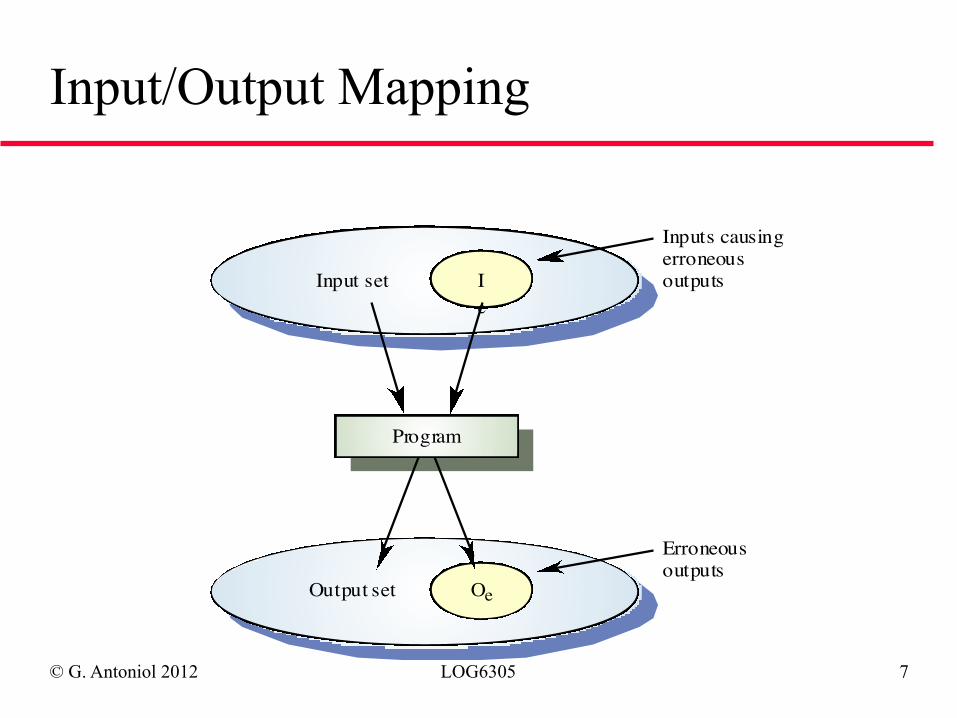
Input/Output Mapping
Ie
Input set
OeOutput set
Program
Inputs causingerroneousoutputs
Erroneousoutputs
© G. Antoniol 2012 LOG6305 8
How Can we Measure and Model Reliability
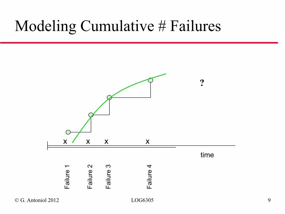
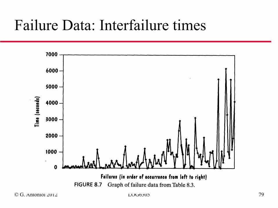
◆ The cumulative number of failures by time t ◆ Failure Intensity: The number of failures per time
unit at time t ◆ Mean-Time-To-Failure MTTF: Average value of
inter-failure time interval ◆ We do not know for sure when the software is
going to fail next => model failure behavior as a random process
© G. Antoniol 2012 LOG6305 9
Modeling Cumulative # Failures
x x x x
time
Failu
re 1
Failu
re 2
Failu
re 3
Failu
re 4
?
© G. Antoniol 2012 LOG6305 10
Reliability Growth
◆ Reliability is improved when software faults which occur in the most frequently used parts of the software are removed
◆ Removing x% of software faults will not necessarily lead to an x% reliability improvement
◆ In a study, removing 60% of software defects actually led to a 3% reliability improvement
◆ Removing faults with serious consequences is the most important objective
© G. Antoniol 2012 LOG6305 11
Problems with Quantification?
◆ US standard for equipment on civil aircraft:
➫ [A critical failure must be ] so unlikely that [it] need not be
considered ever to occur, unless engineering judgment would
require [its] consideration.
◆ Typical requirement for critical flight systems: 10-9 probability of failure per flying hour based on a flight mean duration of 10 hours.
◆ Problem 1: such a level of reliability cannot be demonstrated – would require too much testing time
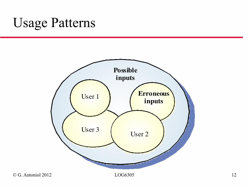
◆ Problem 2: Reliability is relative to the usage of the system
© G. Antoniol 2012 LOG6305 12
Usage Patterns
Possibleinputs
User 1
User 3User 2
Erroneousinputs
© G. Antoniol 2012 LOG6305 13
Reliability and Quality
◆ Reliability is usually more important than other quality aspects
◆ Unreliable software isn't used ◆ Hard to improve the quality of unreliable systems ◆ Software failure costs often far exceed system
costs ◆ Costs of data loss are very high
© G. Antoniol 2012 LOG6305 14
Reliability Metrics
◆ Probability of failure on demand • This is a measure of the likelihood that the system will fail when a
service request is made • POFOD = 0.001 means 1 out of 1000 service requests result in
failure • Relevant for safety-critical or non-stop systems
◆ Rate of fault occurrence (ROCOF) • Frequency of occurrence of unexpected behavior • ROCOF of 0.02 means 2 failures are likely in each 100
operational time units • Relevant for operating systems, transaction processing systems
© G. Antoniol 2012 LOG6305 15
Reliability Metrics
◆ Mean time to failure • Measure of the time between observed failures • MTTF of 500 means that the time between failures is 500 time
units • Relevant for systems with long transactions e.g. CAD systems
◆ Availability • Measure of how likely the system is available for use. Takes
repair/restart time into account • Availability of 0.998 means software is available for 998 out of
1000 time units • Relevant for continuously running systems e.g. telephone
switching systems
© G. Antoniol 2012 LOG6305 16
Reliability Measurement
◆ Measure the number of system failures for a given number of system inputs • Used to compute POFOD
◆ Measure the time (or number of transactions) between system failures • Used to compute ROCOF and MTTF
◆ Measure the time to restart after failure • Used to compute AVAIL
© G. Antoniol 2012 LOG6305 17
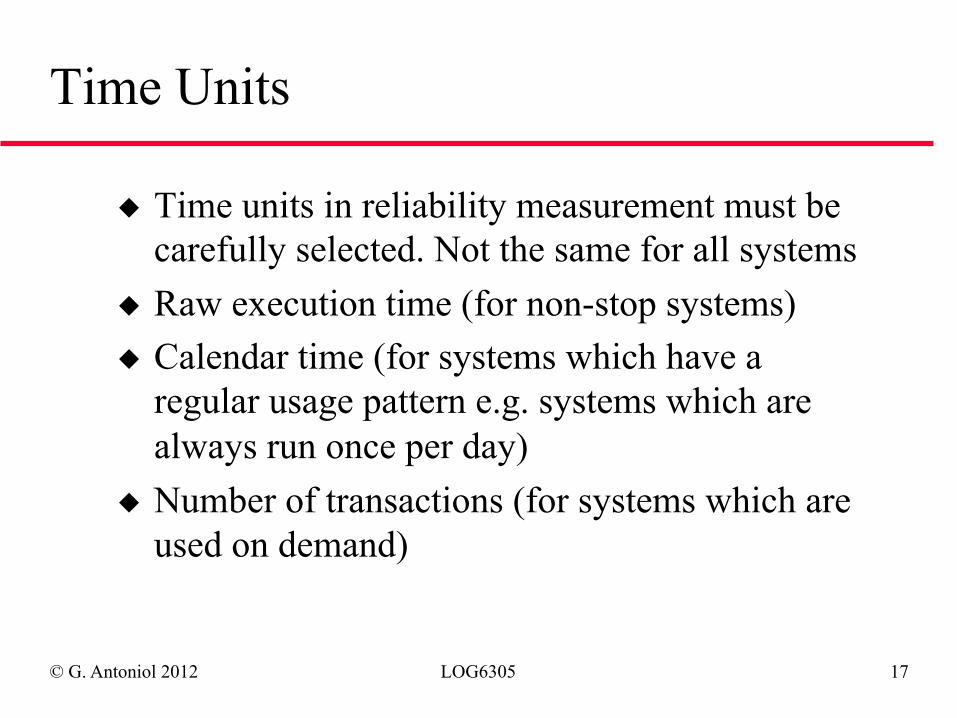
Time Units
◆ Time units in reliability measurement must be carefully selected. Not the same for all systems
◆ Raw execution time (for non-stop systems) ◆ Calendar time (for systems which have a
regular usage pattern e.g. systems which are always run once per day)
◆ Number of transactions (for systems which are used on demand)
© G. Antoniol 2012 LOG6305 18
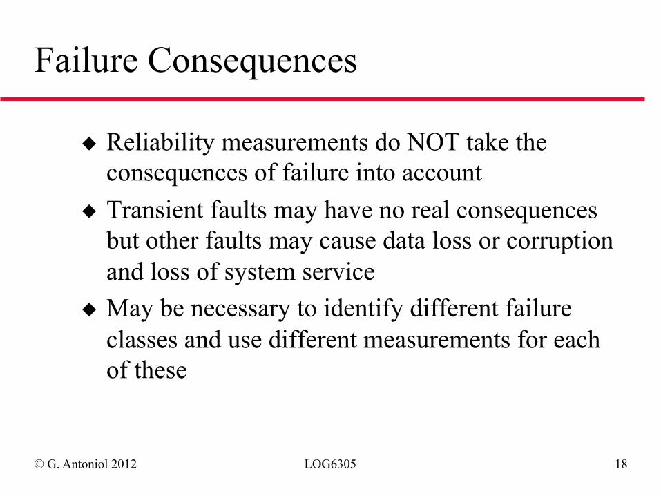
Failure Consequences
◆ Reliability measurements do NOT take the consequences of failure into account
◆ Transient faults may have no real consequences but other faults may cause data loss or corruption and loss of system service
◆ May be necessary to identify different failure classes and use different measurements for each of these
© G. Antoniol 2012 LOG6305 19
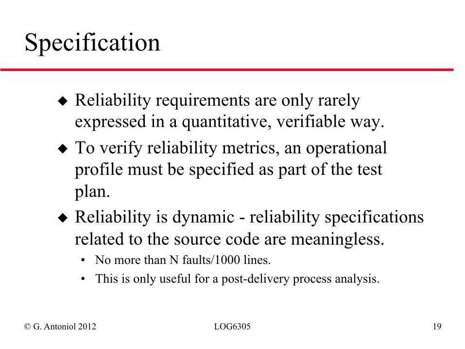
Specification
◆ Reliability requirements are only rarely expressed in a quantitative, verifiable way.
◆ To verify reliability metrics, an operational profile must be specified as part of the test plan.
◆ Reliability is dynamic - reliability specifications related to the source code are meaningless. • No more than N faults/1000 lines. • This is only useful for a post-delivery process analysis.
© G. Antoniol 2012 LOG6305 20
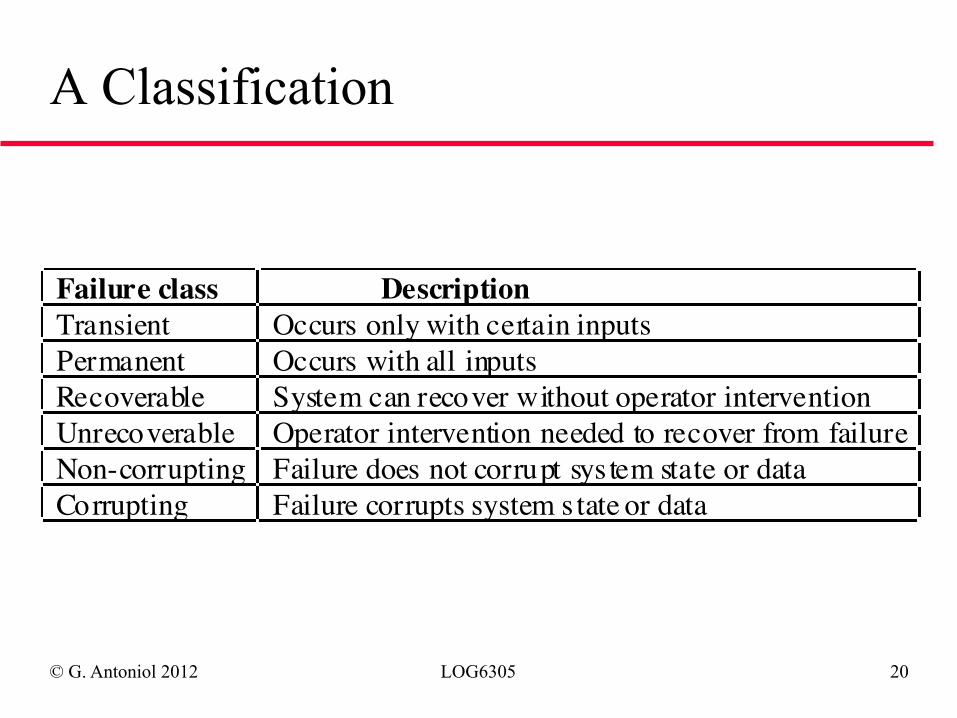
A Classification
Failure class DescriptionTransient Occurs only with certain inputsPermanent Occurs with all inputsRecoverable System can recover without operator interventionUnrecoverable Operator intervention needed to recover from failureNon-corrupting Failure does not corrupt sys tem state or dataCorrupting Failure corrupts system s tate or data
© G. Antoniol 2012 LOG6305 21
Specification Validation
◆ It is impossible to empirically validate very high reliability specifications
◆ No database corruptions means POFOD of less than 1 in 200 million
◆ If a transaction takes 1 second, then simulating one day’s transactions takes 3.5 days
◆ It would take longer than the system’s lifetime to test it for reliability
© G. Antoniol 2012 LOG6305 22
Compromises
◆ Because of very high costs of reliability achievement, it may be more cost effective to accept unreliability (and pay for failure costs)
◆ Social, business and political factors: ➫ A reputation for unreliable products may lose
future business ◆ Depends on system type - for business systems in
particular, modest reliability may be adequate
© G. Antoniol 2012 LOG6305 23
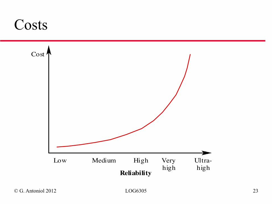
Costs
Cost
Low Medium High Veryhigh
Ultra-high
Reliability
© G. Antoniol 2012 LOG6305 24
Statistical Testing
◆ Testing software for reliability rather than fault detection
◆ Test data selection should follow the predicted usage profile for the software
◆ Measuring the number of errors allows the reliability of the software to be predicted
◆ An acceptable level of reliability should be specified and the software tested and amended until that level of reliability is reached
© G. Antoniol 2012 LOG6305 25
Testing Procedure
◆ Determine operational profile of the software ◆ Generate a set of test data corresponding to
this profile ◆ Apply tests, measuring amount of execution
time between each failure ◆ After a statistically valid number of tests have
been executed, reliability can be measured
© G. Antoniol 2012 LOG6305 26
Difficulties
◆ Uncertainty in the operational profile • This is a particular problem for new systems with no operational
history. Less of a problem for replacement systems
◆ High costs of generating the operational profile • Costs are very dependent on what usage information is collected
by the organisation which requires the profile
◆ Statistical uncertainty when high reliability is specified • Difficult to estimate level of confidence in operational profile • Usage pattern of software may change with time
© G. Antoniol 2012 LOG6305 27
Reliability Growth Model
◆ Growth model is a mathematical model of the system reliability change as it is tested and faults are removed
◆ Used as a means of reliability prediction by extrapolating from current data
◆ Depends on the use of statistical testing to measure the reliability of a system version
© G. Antoniol 2012 LOG6305 28
Reliability Models
◆ Many different reliability growth models have been proposed
◆ No universally applicable growth model ◆ Reliability should be measured and observed data
should be fitted to several models ◆ Best-fit model should be used for reliability
prediction
© G. Antoniol 2012 LOG6305 29
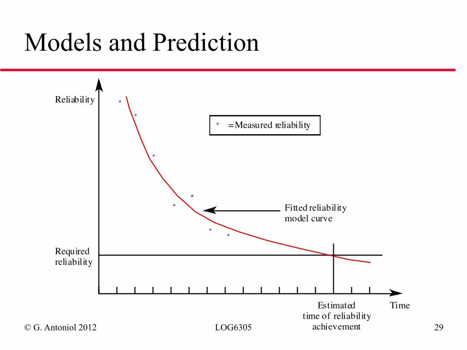
Models and Prediction
Reliability
Requiredreliability
Fitted reliabilitymodel curve
Estimatedtime of reliability
achievement
Time
= Measured reliability
© G. Antoniol 2012 LOG6305 30
Hardware Reliability
◆ Well-developed reliability theories ◆ A hardware component may fail due to design error, poor
fabrication quality, momentary overload, deterioration, etc. ◆ The random nature of system failure enables the estimation
of system reliability using probability theory ◆ Can it be adapted for software? No physical deterioration,
most programs always provide the same answer to the same input, the “fabrication” of code is trivial, etc.
© G. Antoniol 2012 LOG6305 31
Software Reliability Engineering
◆ No method of development can guarantee totally reliable software => important field in practice!
◆ A set of statistical modeling techniques ◆ Enables the achieved reliability to be assessed or
predicted, quantitatively and objectively ◆ Based on observation of system failures during system
testing and operational use ◆ Uses general reliability theory, but is much more than that
© G. Antoniol 2012 LOG6305 32
Applications ◆ How reliable is the program/component now? ◆ Based on the current reliability of a purchased/reused
component: can we accept it or should we reject it? ◆ Based on the current reliability of the system: can we stop
testing and start shipping? ◆ How reliable will the system be, if we continue testing for
some time? ◆ When will the reliability objective be achieved? ◆ How many failures will occur in the field (and when) – to help
plan resources for customer support?
© G. Antoniol 2012 LOG6305 33
Random Variable
◆ A random variable X is a function defined over a sample space S
◆ X associates a real numbers x with each possible outcome in S: X(e) = x
◆ If S is finite or countable infinite we say that X is discrete
◆ If X can be any value in a given interval we say that X is a continuous random variable
© G. Antoniol 2012 LOG6305 34
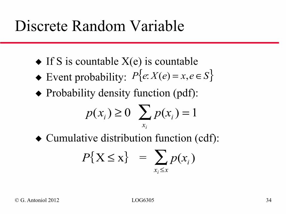
Discrete Random Variable
{ }P e X e x e S: ( ) ,= ∈◆ If S is countable X(e) is countable ◆ Event probability: ◆ Probability density function (pdf):
◆ Cumulative distribution function (cdf):
p x p xix
ii
( ) ( )≥ =∑0 1
{ }P p xx x
ii
X x = ≤≤∑ ( )
© G. Antoniol 2012 LOG6305 35
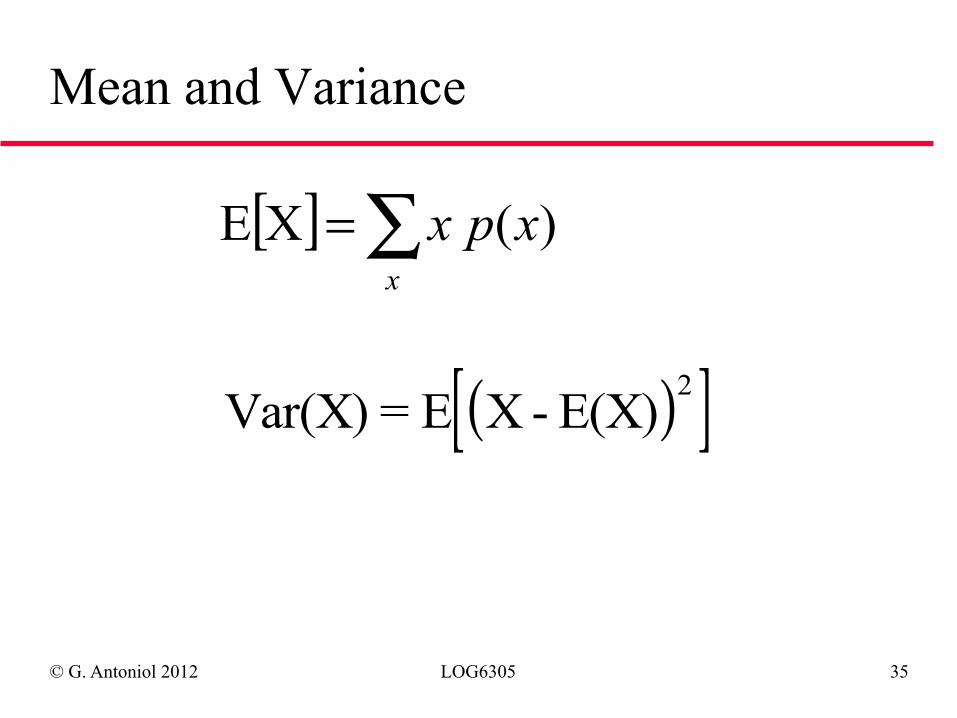
Mean and Variance
[ ] ∑=x
xpx )( XE
( )[ ]Var(X) = E X - E(X) 2
© G. Antoniol 2012 LOG6305 36
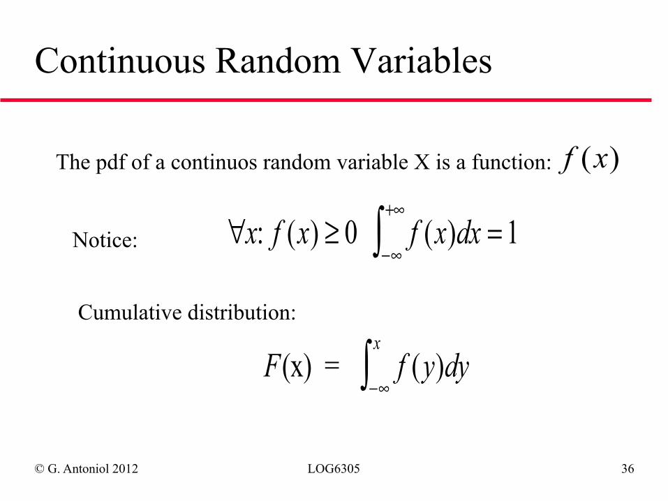
Continuous Random Variables
The pdf of a continuos random variable X is a function: f x( )
Notice: ∀ ≥ =−∞
+∞
∫x f x f x dx: ( ) ( ) 0 1
F f y dyx
(x) = ( )−∞∫
Cumulative distribution:
© G. Antoniol 2012 LOG6305 37
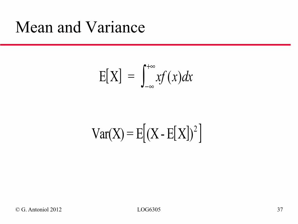
Mean and Variance
[ ]E X = xf x dx( )−∞
+∞
∫
[ ][ ]Var(X) = E (X - E X )2
© G. Antoniol 2012 LOG6305 38
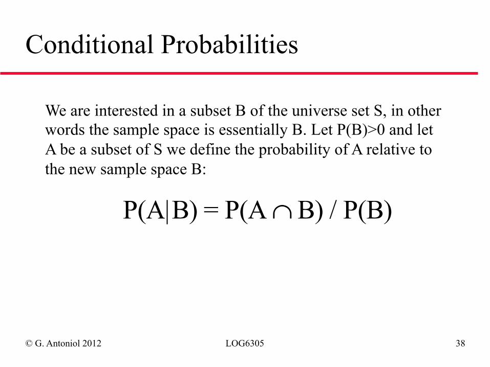
Conditional Probabilities
We are interested in a subset B of the universe set S, in other words the sample space is essentially B. Let P(B)>0 and let A be a subset of S we define the probability of A relative to the new sample space B:
P(A|B) = P(A B) / P(B)∩
© G. Antoniol 2012 LOG6305 39
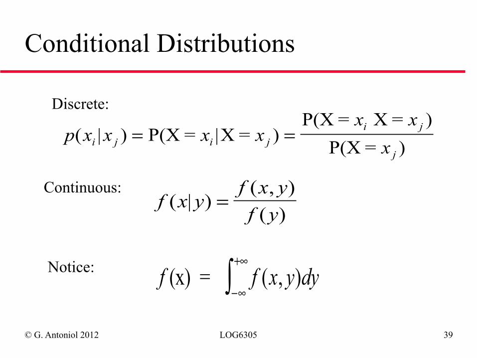
Conditional Distributions
Discrete:
Continuous:
p x x x xx xxi j i j
i j
j( | ) | )
))
= =P(X = X =P(X = X =
P(X =
f x yf x yf y
( | )( , )( )
=
Notice: f f x y dy(x) = ( , )−∞
+∞
∫
© G. Antoniol 2012 LOG6305 40
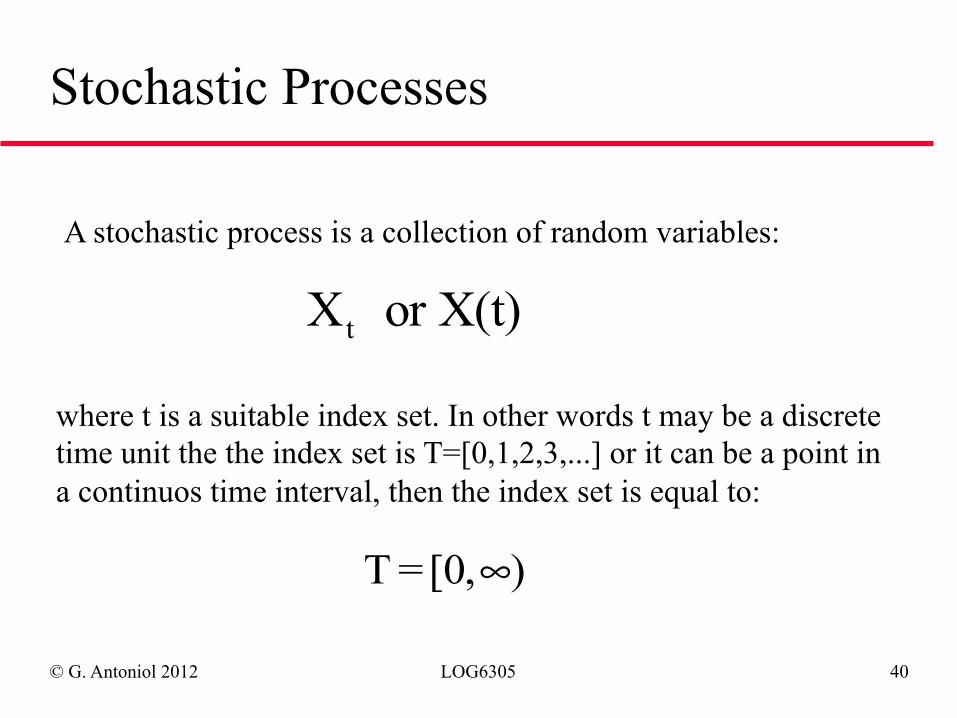
Stochastic Processes
A stochastic process is a collection of random variables:
X or X(t)t
where t is a suitable index set. In other words t may be a discrete time unit the the index set is T=[0,1,2,3,...] or it can be a point in a continuos time interval, then the index set is equal to:
T=[0, )∞

© G. Antoniol 2012 LOG6305 41
Reliability
The random variable of interest is the time to failure T. We focus our interest on the probability that the time to failure between is in some interval. The time to failure T in some interval:
T (t , t + t)∈ ΔIn other words:
P(t T t + t) = (t) t = (t + t) - (t)≤ ≤ Δ Δ Δf F F
The pdf f is also called failure density function
© G. Antoniol 2012 LOG6305 42
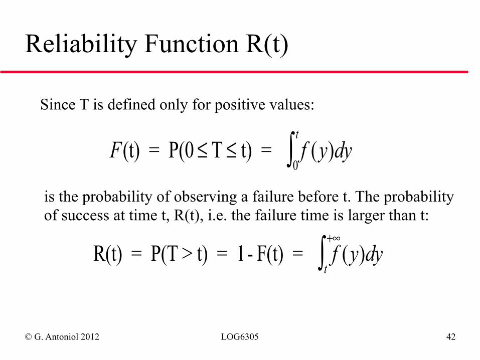
Reliability Function R(t)
Since T is defined only for positive values:
F f y dyt
(t) = P(0 T t) = ≤ ≤ ∫ ( )0
is the probability of observing a failure before t. The probability of success at time t, R(t), i.e. the failure time is larger than t:
R(t) = P(T > t) = 1- F(t) = f y dyt
( )+∞
∫
© G. Antoniol 2012 LOG6305 43
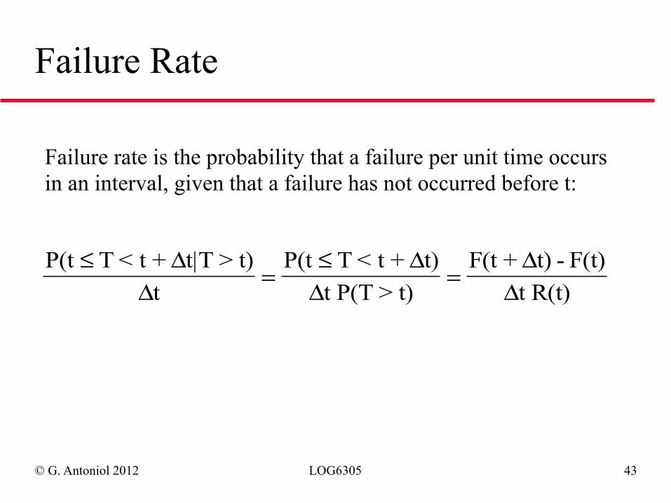
Failure Rate
Failure rate is the probability that a failure per unit time occurs in an interval, given that a failure has not occurred before t:
P(t T < t + t|T > t)t
P(t T < t + t)t P(T > t)
F(t + t) - F(t)t R(t)
≤=
≤=
ΔΔ
ΔΔ
ΔΔ
© G. Antoniol 2012 LOG6305 44
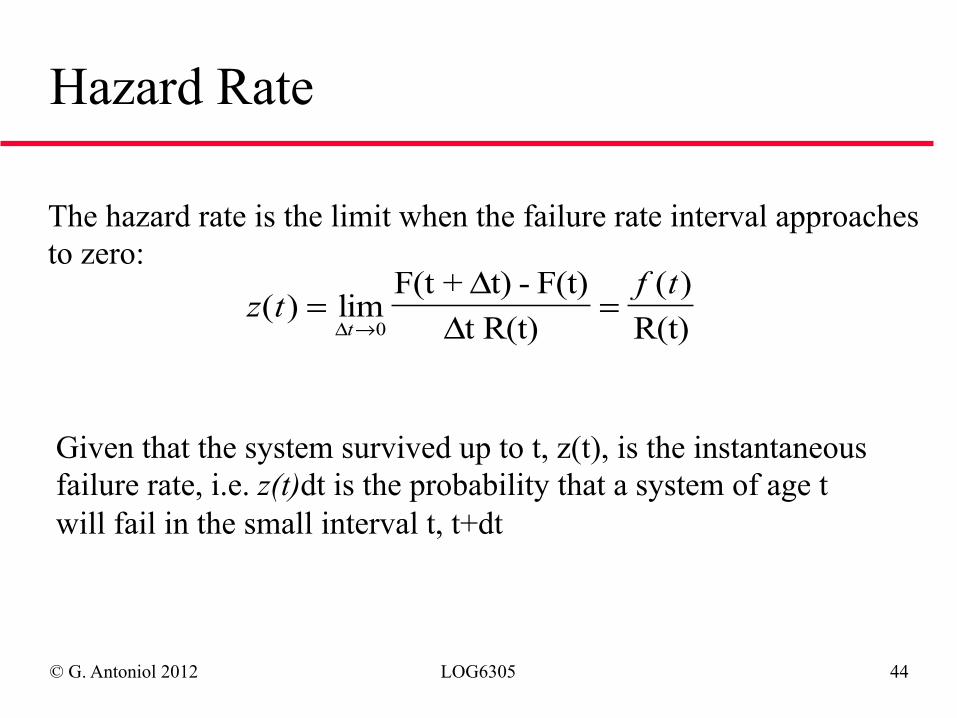
Hazard Rate
The hazard rate is the limit when the failure rate interval approaches to zero:
z tf t
t( ) lim
( )= =
→Δ
ΔΔ0
F(t + t) - F(t)t R(t) R(t)
Given that the system survived up to t, z(t), is the instantaneous failure rate, i.e. z(t)dt is the probability that a system of age t will fail in the small interval t, t+dt
© G. Antoniol 2012 LOG6305 45
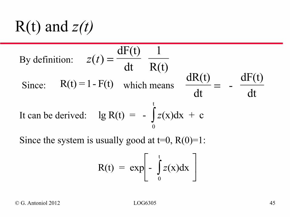
R(t) and z(t)
By definition: z t( ) =dF(t)
dt
1R(t)
Since: R(t) =1- F(t) which means dR(t)
dt -
dF(t)dt
=
It can be derived: lg R(t) = - (x)dx + c0
t
z∫Since the system is usually good at t=0, R(0)=1:
R(t) = exp - (x)dx 0
t
z∫⎡
⎣⎢
⎤
⎦⎥
© G. Antoniol 2012 LOG6305 46
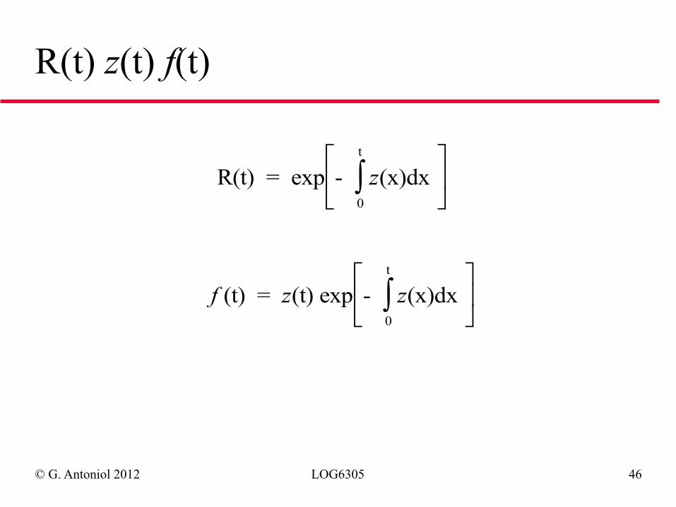
R(t) z(t) f(t)
R(t) = exp - (x)dx 0
t
z∫⎡
⎣⎢
⎤
⎦⎥
(t) = (t) exp - (x)dx 0
t
f z z∫⎡
⎣⎢
⎤
⎦⎥
© G. Antoniol 2012 LOG6305 47
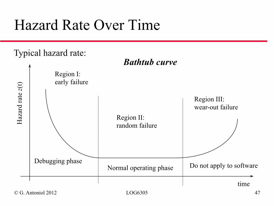
Hazard Rate Over Time
Typical hazard rate:
Region I: early failure
Region II: random failure
Region III: wear-out failure
time
Haz
ard
rate
z(t)
Debugging phase Normal operating phase Do not apply to software
Bathtub curve
© G. Antoniol 2012 LOG6305 48
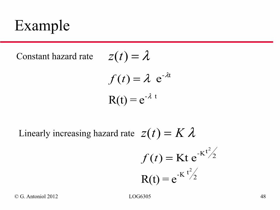
Example
Constant hazard rate
Linearly increasing hazard rate
z t( ) = λf t( ) = λ λ e- t
R(t) = e- tλ
z t K( ) = λ
f t( ) = Kt e-Kt2
2
R(t) = e-K t2
2
© G. Antoniol 2012 LOG6305 49
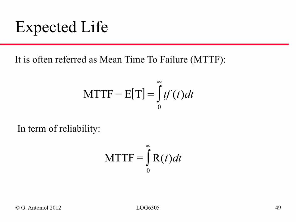
Expected Life
It is often referred as Mean Time To Failure (MTTF):
[ ]MTTF= E T =∞
∫ tf t dt( )0
In term of reliability:
MTTF = R( )t dt0
∞
∫
© G. Antoniol 2012 LOG6305 50
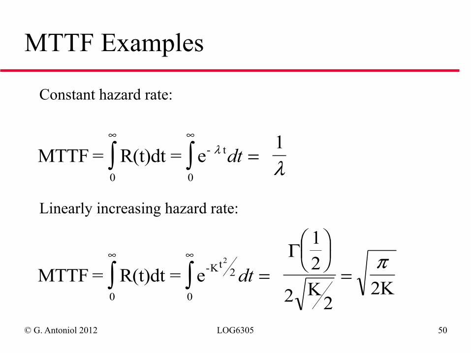
MTTF Examples
Constant hazard rate:
Linearly increasing hazard rate:
MTTF = R(t)dt = e 1- t
00
λ
λdt =∞∞
∫∫
MTTF = R(t)dt = e
12K
22K
-Kt2
00
2
dt =
⎛⎝⎜
⎞⎠⎟=
∞∞
∫∫Γ
2
π
© G. Antoniol 2012 LOG6305 51
Another Point of View
Instead of the random variable T, the time to next failure, we can model with the number of failure a system experienced by time t.
Clearly the number of failure experienced by time t is a random variable, actually it is a random process, since once fixed the time the number of experienced failures is a random variable.
© G. Antoniol 2012 LOG6305 52
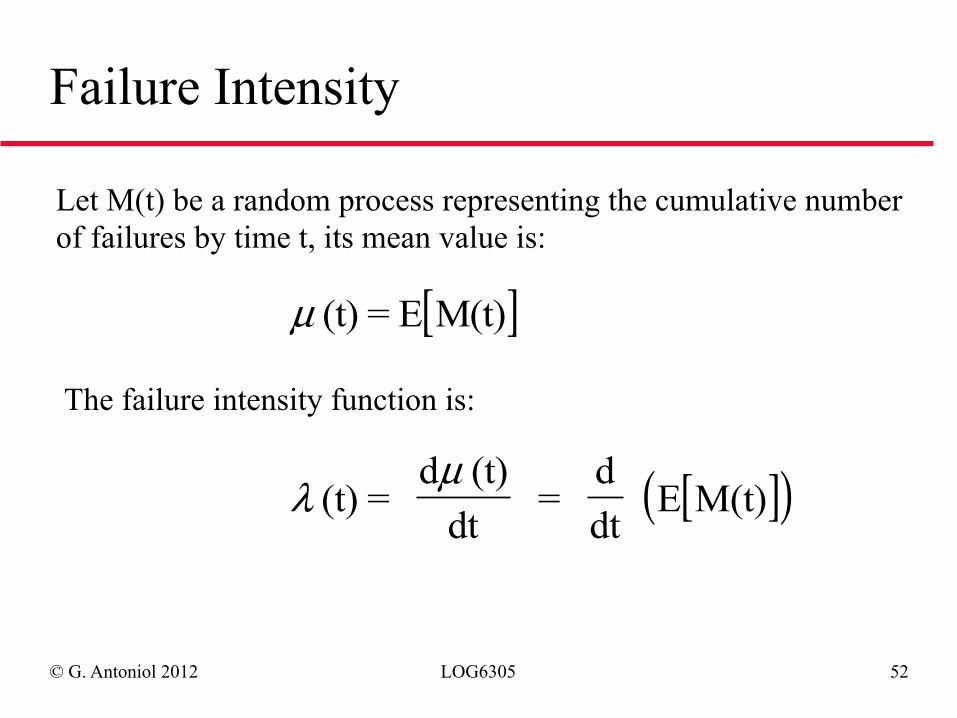
Failure Intensity
Let M(t) be a random process representing the cumulative number of failures by time t, its mean value is:
[ ]µ (t) = E M(t)
The failure intensity function is:
[ ]( )λµ
(t) = d (t)
dt =
ddt
E M(t)
© G. Antoniol 2012 LOG6305 53
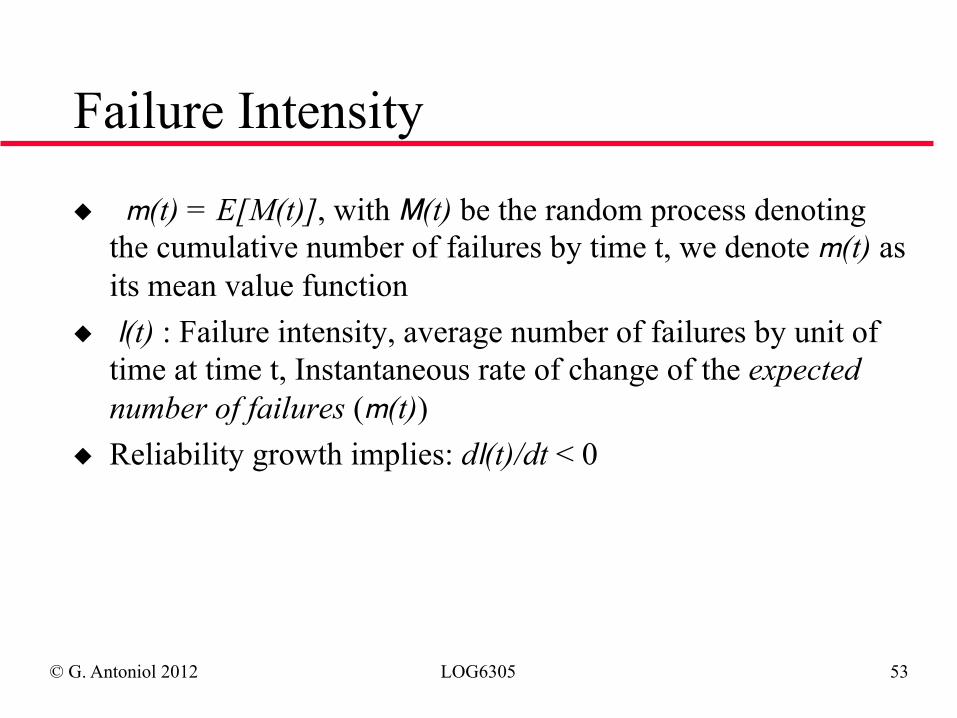
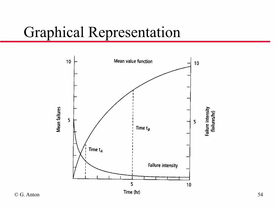
Failure Intensity
◆ m(t) = E[M(t)], with M(t) be the random process denoting the cumulative number of failures by time t, we denote m(t) as its mean value function
◆ l(t) : Failure intensity, average number of failures by unit of time at time t, Instantaneous rate of change of the expected number of failures (m(t))
◆ Reliability growth implies: dl(t)/dt < 0
© G. Antoniol 2012 LOG6305 54
Graphical Representation
© G. Antoniol 2012 LOG6305 55
Failure Intensity Properties
The failure intensity represent the expected number of failures per unit of time.
The number of failures that will occur between t and t + tΔcan be approximated by λ (t) tΔ
While µ (t) is a non decreasing function, it is the cumulative number of failures at t, the failure intensity, its derivative, must decrease in order to obtain an increase in R(t)
© G. Antoniol 2012 LOG6305 56
Reliability Models Classification
◆ Time domain: wall clock versus execution time ◆ Category: the total number of failure that can be
experienced in infinite time (finite or infinite) ◆ Type: the distribution of the number of failures
experienced by time t (Poisson or Binomial)
© G. Antoniol 2012 LOG6305 57
Poisson Type
The distribution of the failure experienced by time t is a Poisson process. In other words if:
t t t t t0 1 2 n= =0, , ,...,
is a partition of the interval [0,t] we have a Poisson process if the number of faults detected in the i-th interval are independent Poissons variables with f i i = 1,2,..., n
[ ]E (t (ti i i-1f = −µ µ) )
© G. Antoniol 2012 LOG6305 58
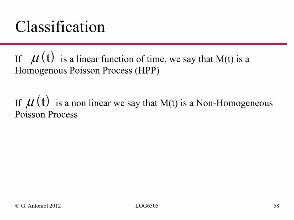
Classification
If is a linear function of time, we say that M(t) is a Homogenous Poisson Process (HPP)
If is a non linear we say that M(t) is a Non-Homogeneous Poisson Process
( )µ t
( )µ t
© G. Antoniol 2012 LOG6305 59
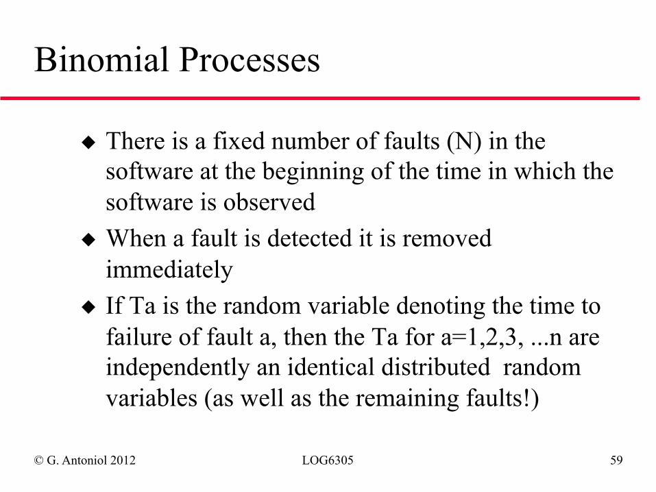
Binomial Processes
◆ There is a fixed number of faults (N) in the software at the beginning of the time in which the software is observed
◆ When a fault is detected it is removed immediately
◆ If Ta is the random variable denoting the time to failure of fault a, then the Ta for a=1,2,3, ...n are independently an identical distributed random variables (as well as the remaining faults!)
© G. Antoniol 2012 LOG6305 60
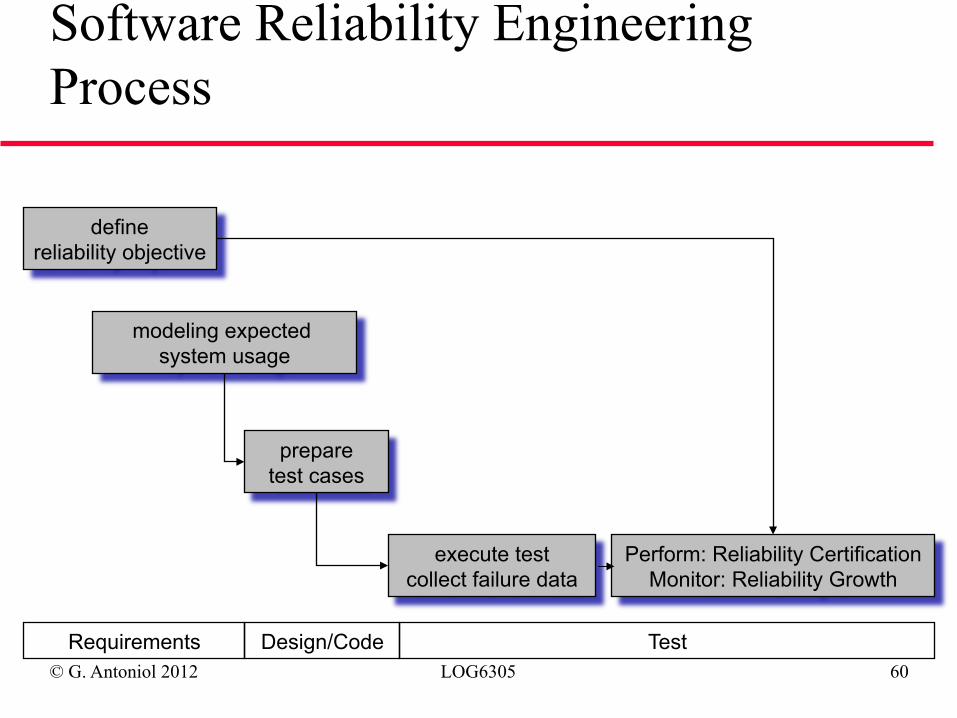
define reliability objective
modeling expected system usage
prepare test cases
execute test collect failure data
Perform: Reliability Certification Monitor: Reliability Growth
Requirements Design/Code Test
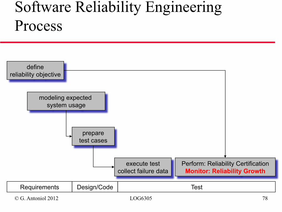
Software Reliability Engineering Process
© G. Antoniol 2012 LOG6305 61
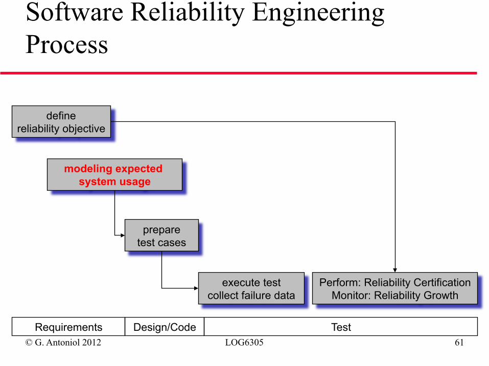
define reliability objective
modeling expected system usage
prepare test cases
execute test collect failure data
Perform: Reliability Certification Monitor: Reliability Growth
Requirements Design/Code Test
Software Reliability Engineering Process
© G. Antoniol 2012 LOG6305 62
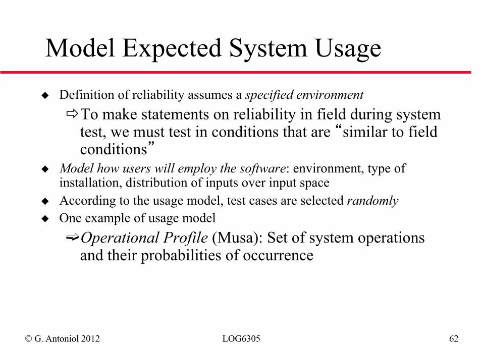
Model Expected System Usage ◆ Definition of reliability assumes a specified environment
ð To make statements on reliability in field during system test, we must test in conditions that are “similar to field conditions”
◆ Model how users will employ the software: environment, type of installation, distribution of inputs over input space
◆ According to the usage model, test cases are selected randomly ◆ One example of usage model ➫ Operational Profile (Musa): Set of system operations
and their probabilities of occurrence
© G. Antoniol 2012 LOG6305 63
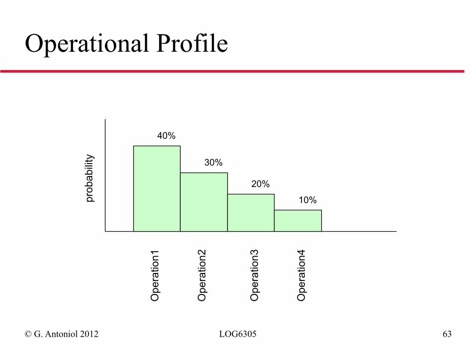
Operational Profile
Ope
ratio
n1
Ope
ratio
n2
Ope
ratio
n3
Ope
ratio
n4
prob
abili
ty
10%
20%
30%
40%
© G. Antoniol 2012 LOG6305 64
Operations
◆ Major system logical task of short duration, which returns control to the system when complete and whose processing is substantially different from other operations ➫ major: related to functional requirement (similar to use
cases) ➫ logical: not bound to software, hardware, users,
machines ➫ short: 100s-1000s operations per hour under normal
load conditions ➫ different: likely to contain different faults
◆ In OO systems, an operation ~ use case
© G. Antoniol 2012 LOG6305 65
Examples
◆ Command executed by a user ◆ Response to an input from an external system or
device, e.g., processing a transaction, processing an event (alarm)
◆ Routine housekeeping, e.g., file backup, database cleanup
© G. Antoniol 2012 LOG6305 66
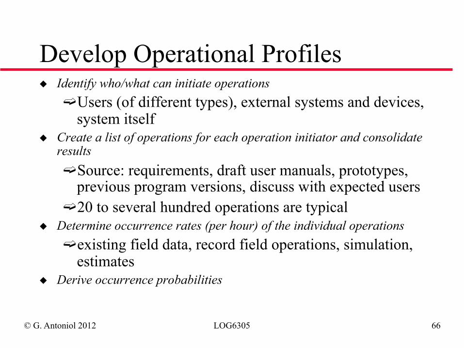
Develop Operational Profiles ◆ Identify who/what can initiate operations ➫ Users (of different types), external systems and devices,
system itself ◆ Create a list of operations for each operation initiator and consolidate
results ➫ Source: requirements, draft user manuals, prototypes,
previous program versions, discuss with expected users ➫ 20 to several hundred operations are typical
◆ Determine occurrence rates (per hour) of the individual operations ➫ existing field data, record field operations, simulation,
estimates ◆ Derive occurrence probabilities
© G. Antoniol 2012 LOG6305 67
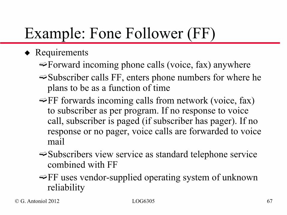
Example: Fone Follower (FF) ◆ Requirements ➫ Forward incoming phone calls (voice, fax) anywhere ➫ Subscriber calls FF, enters phone numbers for where he
plans to be as a function of time ➫ FF forwards incoming calls from network (voice, fax)
to subscriber as per program. If no response to voice call, subscriber is paged (if subscriber has pager). If no response or no pager, voice calls are forwarded to voice mail
➫ Subscribers view service as standard telephone service combined with FF
➫ FF uses vendor-supplied operating system of unknown reliability
© G. Antoniol 2012 LOG6305 68
Initiators of Operations
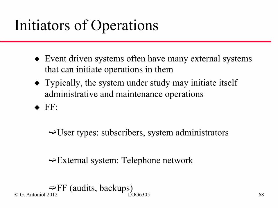
◆ Event driven systems often have many external systems that can initiate operations in them
◆ Typically, the system under study may initiate itself administrative and maintenance operations
◆ FF:
➫ User types: subscribers, system administrators
➫ External system: Telephone network
➫ FF (audits, backups)
© G. Antoniol 2012 LOG6305 69
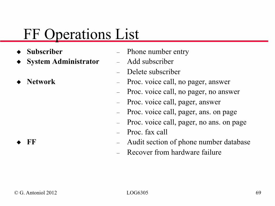
FF Operations List ◆ Subscriber ◆ System Administrator
◆ Network
◆ FF
– Phone number entry – Add subscriber – Delete subscriber – Proc. voice call, no pager, answer – Proc. voice call, no pager, no answer – Proc. voice call, pager, answer – Proc. voice call, pager, ans. on page – Proc. voice call, pager, no ans. on page – Proc. fax call – Audit section of phone number database – Recover from hardware failure
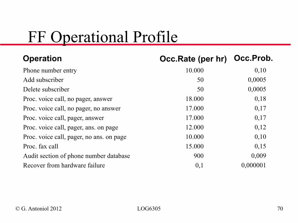
© G. Antoniol 2012 LOG6305 70
FF Operational Profile
10.000 50 50
18.000 17.000 17.000 12.000 10.000 15.000
900 0,1
Phone number entry Add subscriber Delete subscriber Proc. voice call, no pager, answer Proc. voice call, no pager, no answer Proc. voice call, pager, answer Proc. voice call, pager, ans. on page Proc. voice call, pager, no ans. on page Proc. fax call Audit section of phone number database Recover from hardware failure
0,10 0,0005 0,0005
0,18 0,17 0,17 0,12 0,10 0,15
0,009 0,000001
Operation Occ.Rate (per hr) Occ.Prob.
© G. Antoniol 2012 LOG6305 71
Statistical Testing
◆ Testing based on operational profiles is referred to as statistical testing ◆ This form of testing has the advantage of testing more intensively the
system functions that will be used the most ◆ Good for reliability estimation, but not very effective in terms of
finding defects ◆ Hence we differentiate testing that aims at finding defects
(verification) and testing whose purpose is reliability assessment (validation).
◆ There exists research on techniques that combine white-box testing and statistical testing …
© G. Antoniol 2012 LOG6305 72
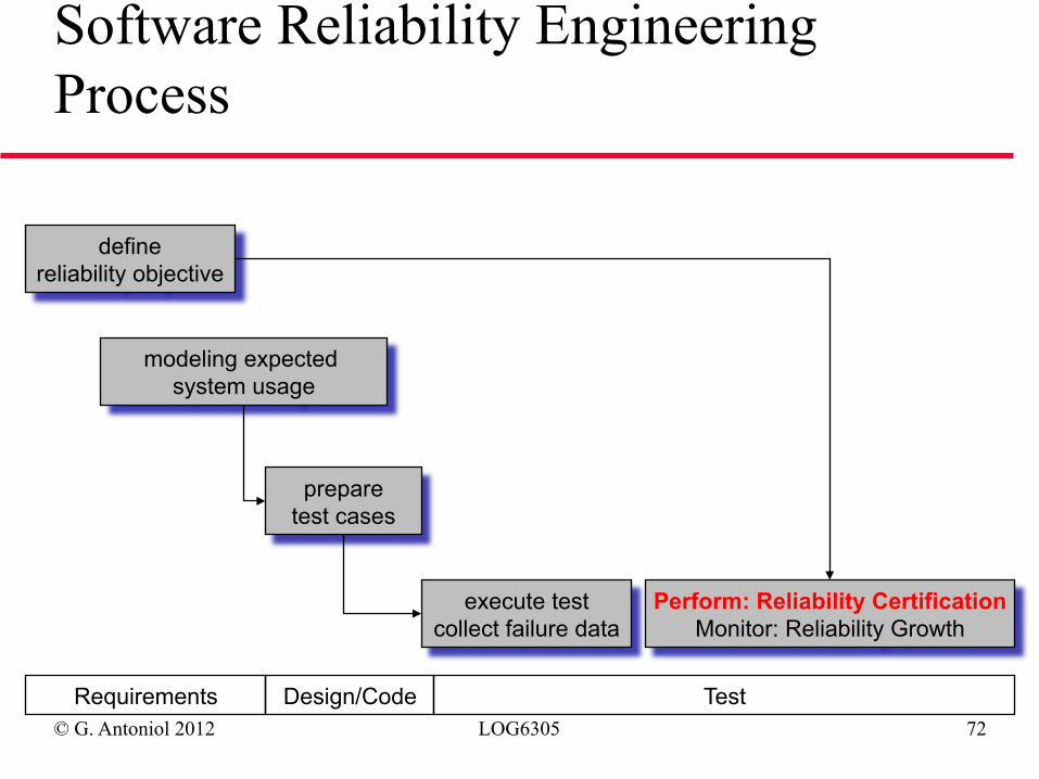
define reliability objective
modeling expected system usage
prepare test cases
execute test collect failure data
Perform: Reliability Certification Monitor: Reliability Growth
Requirements Design/Code Test
Software Reliability Engineering Process
© G. Antoniol 2012 LOG6305 73
Can We Accept a Component?
◆ Certification Testing: Show that a (acquired or developed) component satisfies a given reliability objective (e.g., failure intensity)
◆ Generate test data randomly according to usage model (e.g., operational profile)
◆ Record all failures (also multiple ones) but do not correct
© G. Antoniol 2012 LOG6305 74
Procedure
◆ Use a hypothesis testing control chart to show that the reliability objective is/is not satisfied
➫ Reliability Demonstration Chart
» Collect times at which failures occurred » Normalize data by multiplying with failure intensity
objective (using same units!) » Plot each failure in chart » Based on region in which failure falls, accept or
reject component
© G. Antoniol 2012 LOG6305 75
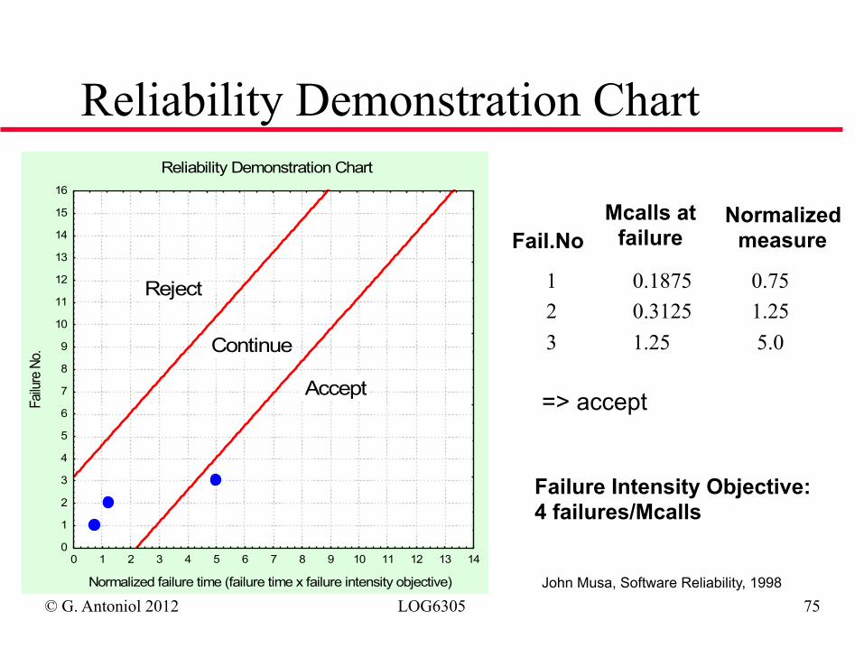
Reliability Demonstration Chart
John Musa, Software Reliability, 1998
1 0.1875 0.75 2 0.3125 1.25 3 1.25 5.0
Fail.No Mcalls at
failure Normalized
measure
Failure Intensity Objective: 4 failures/Mcalls
=> accept
Reliability Demonstration Chart
Normalized failure time (failure time x failure intensity objective)
Failu
re N
o.
0
1
2
3
4
5
6
7
8
9
10
11
12
13
14
15
16
0 1 2 3 4 5 6 7 8 9 10 11 12 13 14
Accept
Reject
Continue
© G. Antoniol 2012 LOG6305 76
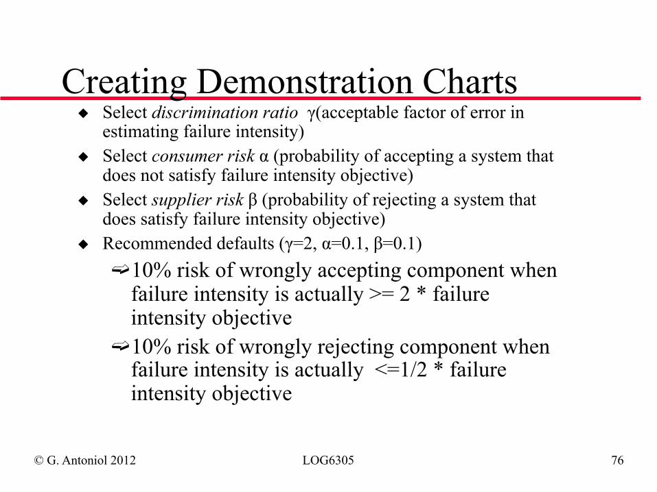
Creating Demonstration Charts ◆ Select discrimination ratio γ(acceptable factor of error in
estimating failure intensity) ◆ Select consumer risk α (probability of accepting a system that
does not satisfy failure intensity objective) ◆ Select supplier risk β (probability of rejecting a system that
does satisfy failure intensity objective) ◆ Recommended defaults (γ=2, α=0.1, β=0.1)
➫ 10% risk of wrongly accepting component when failure intensity is actually >= 2 * failure intensity objective
➫ 10% risk of wrongly rejecting component when failure intensity is actually <=1/2 * failure intensity objective
© G. Antoniol 2012 LOG6305 77
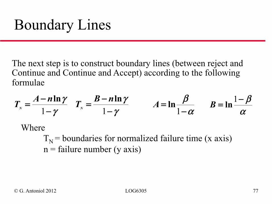
Boundary Lines
γγ
−−=1lnnATN γ
γ−
−=1lnnBTN α
β−
=1
lnAαβ−= 1lnB
Where TN = boundaries for normalized failure time (x axis) n = failure number (y axis)
The next step is to construct boundary lines (between reject and Continue and Continue and Accept) according to the following formulae
© G. Antoniol 2012 LOG6305 78
define reliability objective
modeling expected system usage
prepare test cases
execute test collect failure data
Perform: Reliability Certification Monitor: Reliability Growth
Requirements Design/Code Test
Software Reliability Engineering Process
© G. Antoniol 2012 LOG6305 79
Failure Data: Interfailure times
© G. Antoniol 2012 LOG6305 80
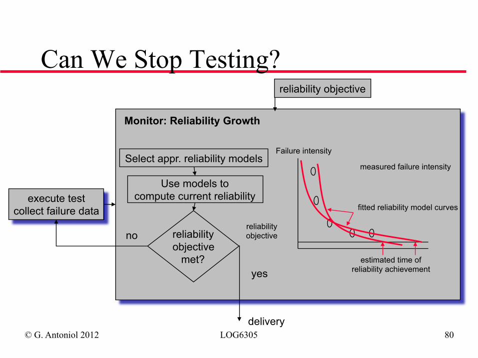
execute test collect failure data
Failure intensity
measured failure intensity
reliability objective
fitted reliability model curves
estimated time of reliability achievement
Monitor: Reliability Growth
Select appr. reliability models
Use models to compute current reliability
reliability objective
met?
reliability objective
no
yes
delivery
Can We Stop Testing?
© G. Antoniol 2012 LOG6305 81
MUSA Model
◆ Developed by John Musa at ATT Bell Labs ◆ One of the first proposed and still widely applied ◆ It is based on execution time ◆ Execution time can be converted into calendar
time ( in a second part of the model)
© G. Antoniol 2012 LOG6305 82
Basic Assumptions
◆ The rate of fault detection is proportional to the current number of faults in the code
◆ The fault detection rate remains constant over the interval between faults occurrence
◆ A fault is corrected instantaneously, without introducing new faults in the code
◆ The failure when the faults are detected are independent ◆ The software is operated in a similar manner as that in
which reliability predictions are made ◆ Every fault has the same change of being encountered
within a severity class as any other fault in that class
© G. Antoniol 2012 LOG6305 83
MUSA Assumptions
◆ Basic assumptions ◆ The cumulative number of failure by time t, M(t),
follows a Poisson process with mean functions:
◆ The execution times between failure are piecewise exponentially distributes, i.e. the hazard rate is a constant
[ ]µ β ββ (t) = with 0 t
0,11 01− >−e
© G. Antoniol 2012 LOG6305 84
MUSA Assumptions ...
◆ Resources available (testing personnel, debuggers, programmers) are constant over the segment of time for which the system is observed
◆ Fault-identification personnel can be fully utilized and computer utilization is constant
◆ Fault-correction personnel is established by the limitation of fault queue length for any fault correction person.
© G. Antoniol 2012 LOG6305 85
MUSA Required Data
◆ To apply MUSA model we need
➫ the actual time that software failed or
➫ the elapsed time between failures
© G. Antoniol 2012 LOG6305 86
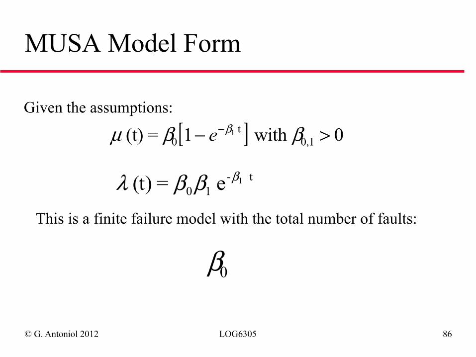
MUSA Model Form
Given the assumptions:
[ ]µ β ββ (t) = with 0 t
0,11 01− >−e
t-10
1e = (t) βββλThis is a finite failure model with the total number of faults:
β0
© G. Antoniol 2012 LOG6305 87
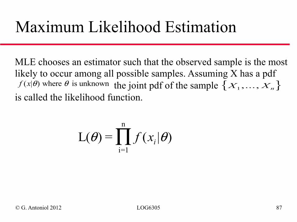
Maximum Likelihood Estimation
MLE chooses an estimator such that the observed sample is the most likely to occur among all possible samples. Assuming X has a pdf the joint pdf of the sample is called the likelihood function. f x( | )θ θ where is unknown { }X Xn1,...,
L( ) =i=1
n
θ θf xi( | )∏
© G. Antoniol 2012 LOG6305 88
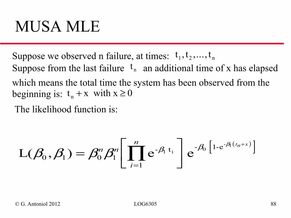
MUSA MLE
Suppose we observed n failure, at times: t t t1 2 n, ,...,Suppose from the last failure t n an additional time of x has elapsed which means the total time the system has been observed from the beginning is: t x with x 0n + ≥
The likelihood function is:
( )[ ]L( e e0- t - 1-e
1 i 0- 1
β β β β β β β
, )1 0 11
=⎡⎣⎢
⎤⎦⎥=
∏+
n n
i
n tn x
© G. Antoniol 2012 LOG6305 89
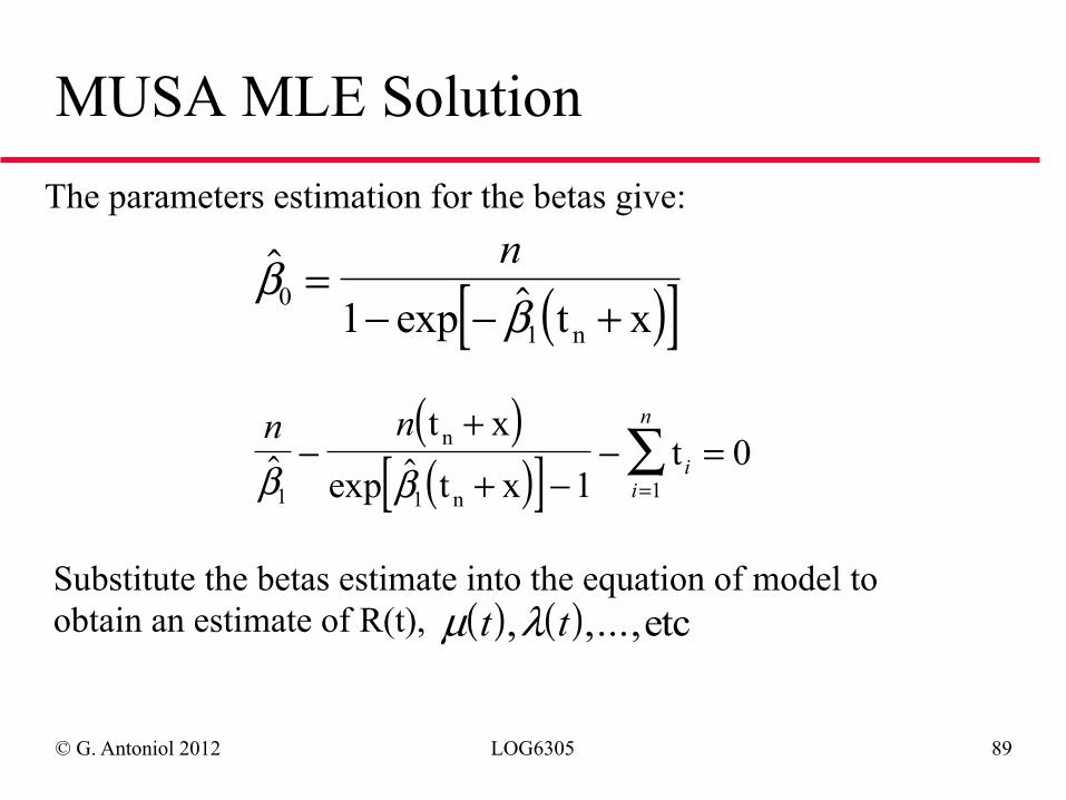
MUSA MLE Solution The parameters estimation for the betas give:
( )[ ]!
exp !β
β011
=− − +
nt xn
( )( )[ ]
n ni
i
n
! exp !β β1 1 110−
+
+ −− =
=∑t x
t xtn
n
Substitute the betas estimate into the equation of model to obtain an estimate of R(t), ( ) ( )µ λt t, ,...,etc
© G. Antoniol 2012 LOG6305 90
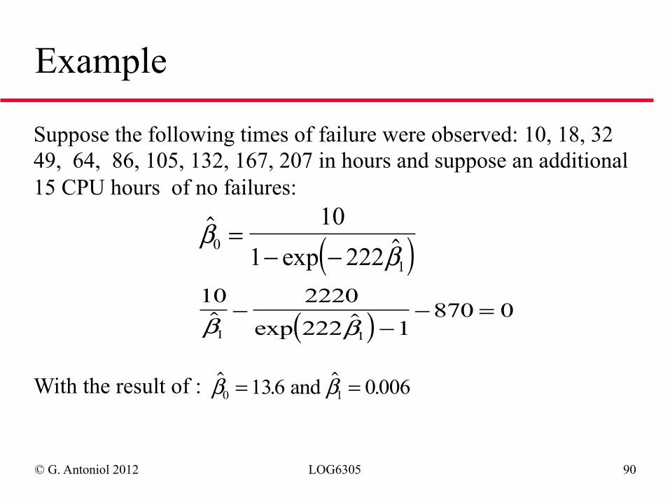
Example
Suppose the following times of failure were observed: 10, 18, 32 49, 64, 86, 105, 132, 167, 207 in hours and suppose an additional 15 CPU hours of no failures:
( )!
exp !β
β01
101 222
=− −
( )10 2220
222 1870 0
1 1! exp !β β−
−− =
With the result of : ! . ! .β β0 1136 0 006= = and
© G. Antoniol 2012 LOG6305 91
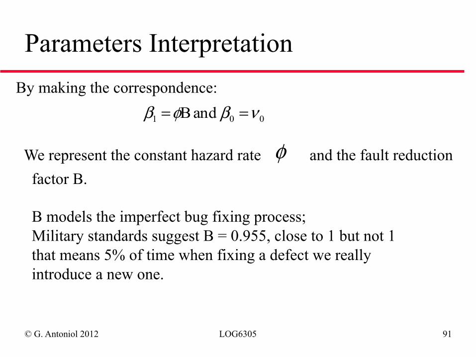
Parameters Interpretation By making the correspondence:
001 and B νβφβ ==
We represent the constant hazard rate φ and the fault reduction factor B. B models the imperfect bug fixing process; Military standards suggest B = 0.955, close to 1 but not 1 that means 5% of time when fixing a defect we really introduce a new one.
© G. Antoniol 2012 LOG6305 92
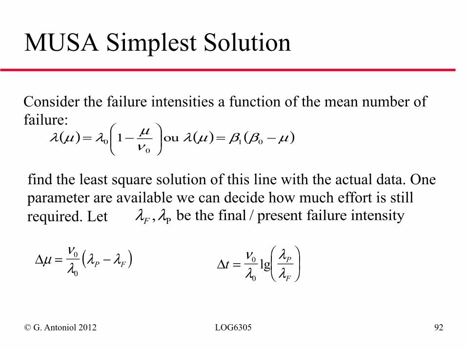
MUSA Simplest Solution
Consider the failure intensities a function of the mean number of failure:
( ) ( ) ( )µββµλνµλµλ −=⎟⎟⎠
⎞⎜⎜⎝
⎛−= 01
00 ou 1
find the least square solution of this line with the actual data. One parameter are available we can decide how much effort is still required. Let λ λF , be the final / present failure intensityP
( )Δµνλ λ λ= −0
0P F Δt P
F=
⎛⎝⎜
⎞⎠⎟
νλ
λλ
0
0lg
© G. Antoniol 2012 LOG6305 93
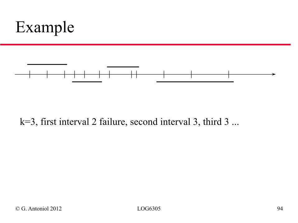
Grouping of Data
◆ Chose a number of failure you wish to consider for each sub-interval say k (suggested k=5)
◆ Divide the data set into p independent sub-sets each containing exactly k failures (p is the smallest integer greater or equal the total number of failure divided by k)
◆ Estimate failure intensity as the ratio between the number of failure in the interval and the interval duration
© G. Antoniol 2012 LOG6305 94
Example
k=3, first interval 2 failure, second interval 3, third 3 ...
© G. Antoniol 2012 LOG6305 95
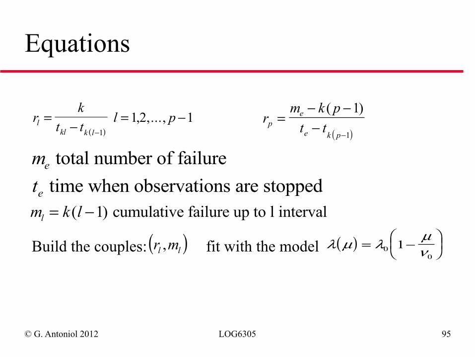
Equations
( )r
kt t
l plkl k l
=−
= −−1
1 2 1 , ,...,( )
rm k pt tpe
e k p
=− −−
−
( )1
1
me total number of failurete time when observations are stoppedm k ll = −( )1 cumulative failure up to l interval
Build the couples: ( )r ml l, fit with the model ( )λ µ λµν= −
⎛⎝⎜
⎞⎠⎟00
1
© G. Antoniol 2012 LOG6305 96
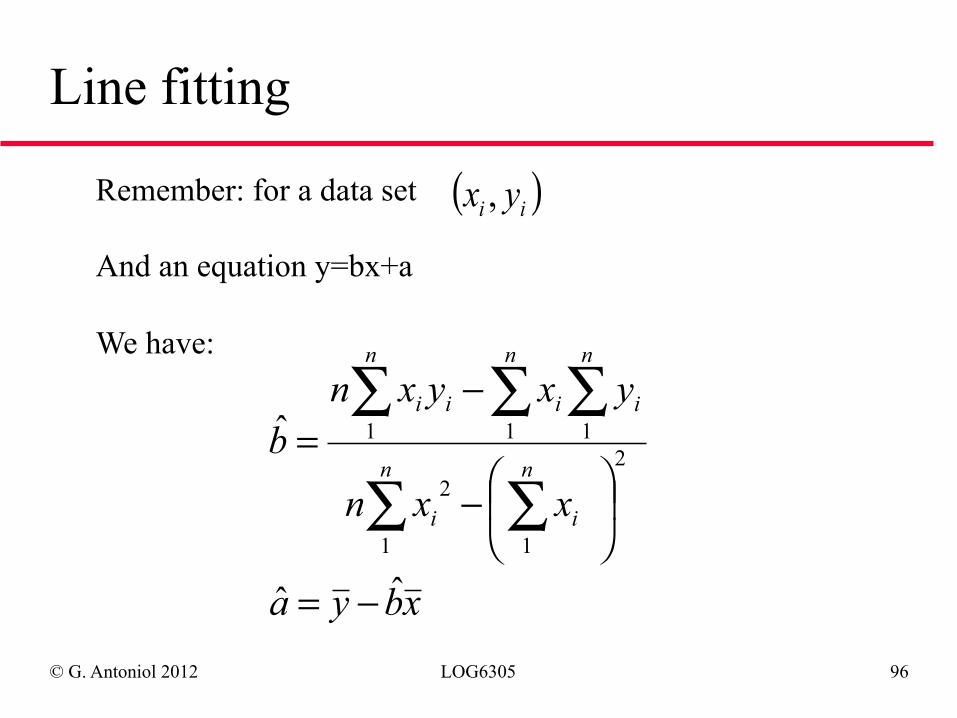
Line fitting
( )ii yx ,Remember: for a data set And an equation y=bx+a We have:
xbya
xxn
yxyxnb
n
i
n
i
n
i
n
i
n
ii
ˆˆ
ˆ2
11
2
111
−=
⎟⎠⎞⎜
⎝⎛−
−=
∑∑
∑∑∑
© G. Antoniol 2012 LOG6305 97
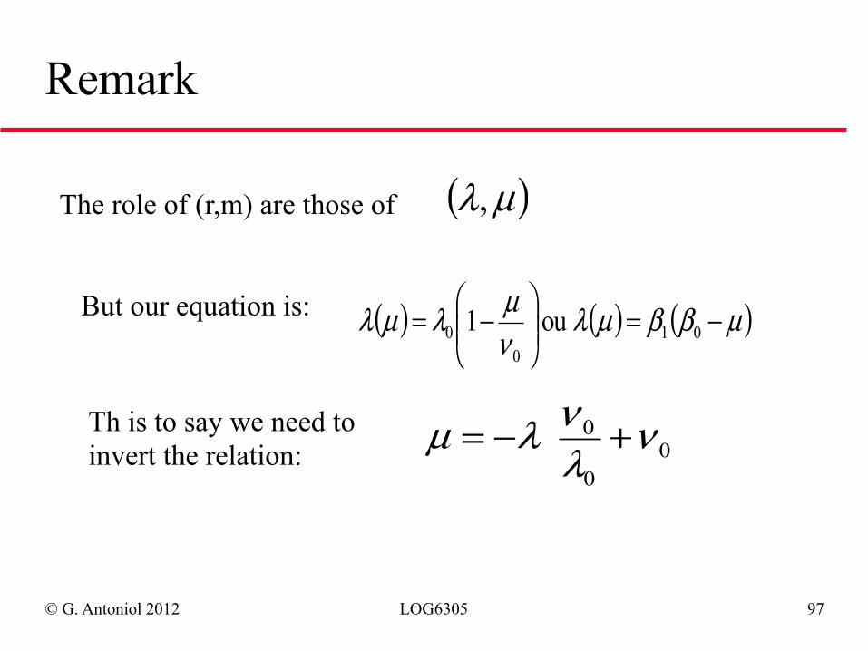
Remark
( )µλ,
( ) ( ) ( )µββµλνµλµλ −=⎟⎟⎠
⎞⎜⎜⎝
⎛−= 01
00 ou 1
The role of (r,m) are those of
But our equation is:
Th is to say we need to invert the relation: 0
0
0 νλνλµ +−=
© G. Antoniol 2012 LOG6305 98
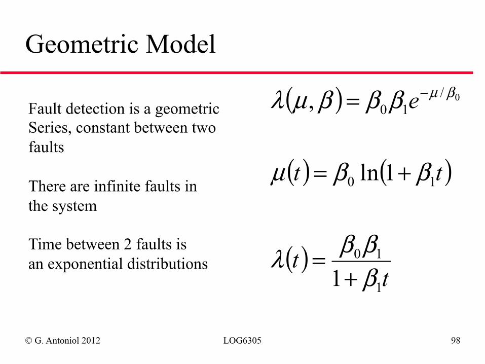
Geometric Model
( )
( ) ( )
( )t
t
tt
e
1
10
10
/10
1
1ln
, 0
βββλ
ββµ
βββµλ βµ
+=
+=
= −Fault detection is a geometric Series, constant between two faults There are infinite faults in the system Time between 2 faults is an exponential distributions
© G. Antoniol 2012 LOG6305 99
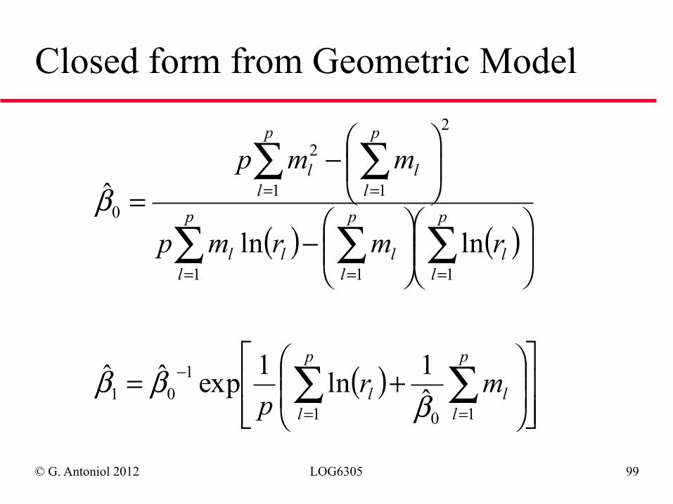
Closed form from Geometric Model
( ) ( )
( )⎥⎥⎦
⎤
⎢⎢⎣
⎡⎟⎟⎠
⎞⎜⎜⎝
⎛+=
⎟⎟⎠
⎞⎜⎜⎝
⎛⎟⎟⎠
⎞⎜⎜⎝
⎛−
⎟⎟⎠
⎞⎜⎜⎝
⎛−
=
∑∑
∑∑∑
∑∑
==
−
===
==
p
ll
p
ll
p
ll
p
ll
p
lll
p
ll
p
ll
mrp
rmrmp
mmp
101
101
111
2
11
2
0
ˆ1ln1expˆˆ
lnln
ˆ
βββ
β
© G. Antoniol 2012 LOG6305 100
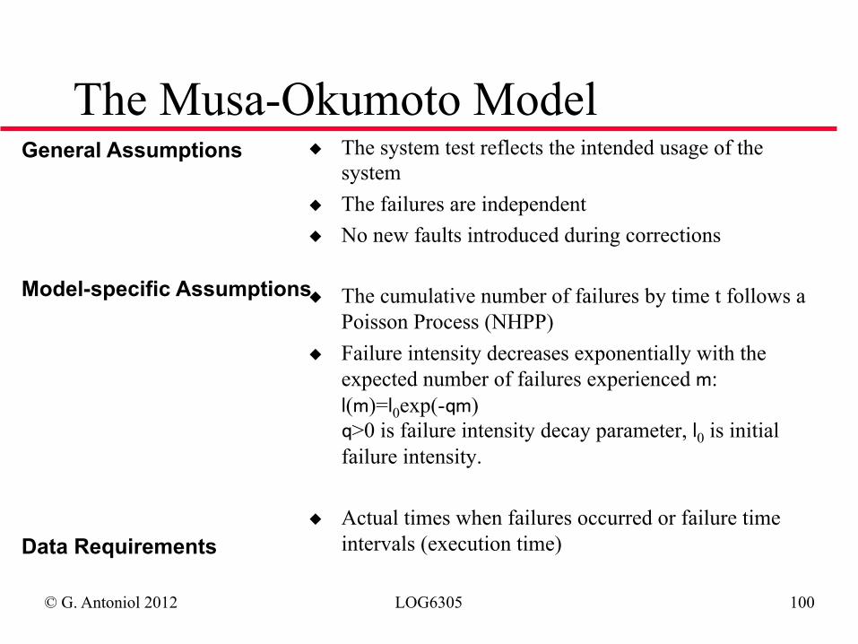
The Musa-Okumoto Model ◆ The system test reflects the intended usage of the
system ◆ The failures are independent ◆ No new faults introduced during corrections
◆ The cumulative number of failures by time t follows a Poisson Process (NHPP)
◆ Failure intensity decreases exponentially with the expected number of failures experienced m: l(m)=l0exp(-qm) q>0 is failure intensity decay parameter, l0 is initial failure intensity.
◆ Actual times when failures occurred or failure time intervals (execution time)
General Assumptions Model-specific Assumptions Data Requirements
© G. Antoniol 2012 LOG6305 101
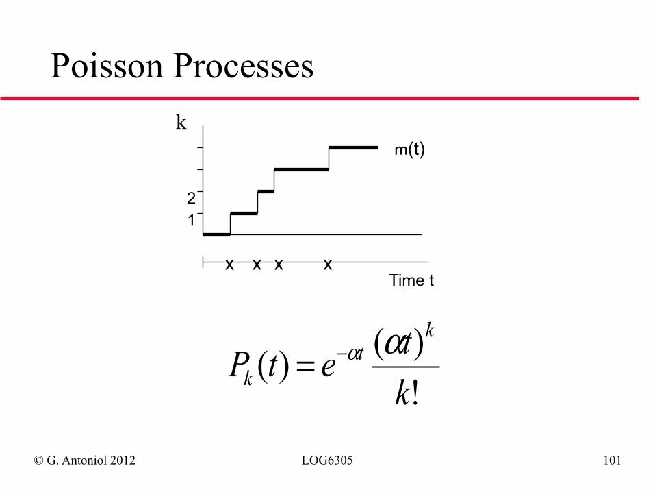
Poisson Processes
x x x x Time t
1 2
m(t)
!)()(ktetPk
tk
αα−=
k
© G. Antoniol 2012 LOG6305 102
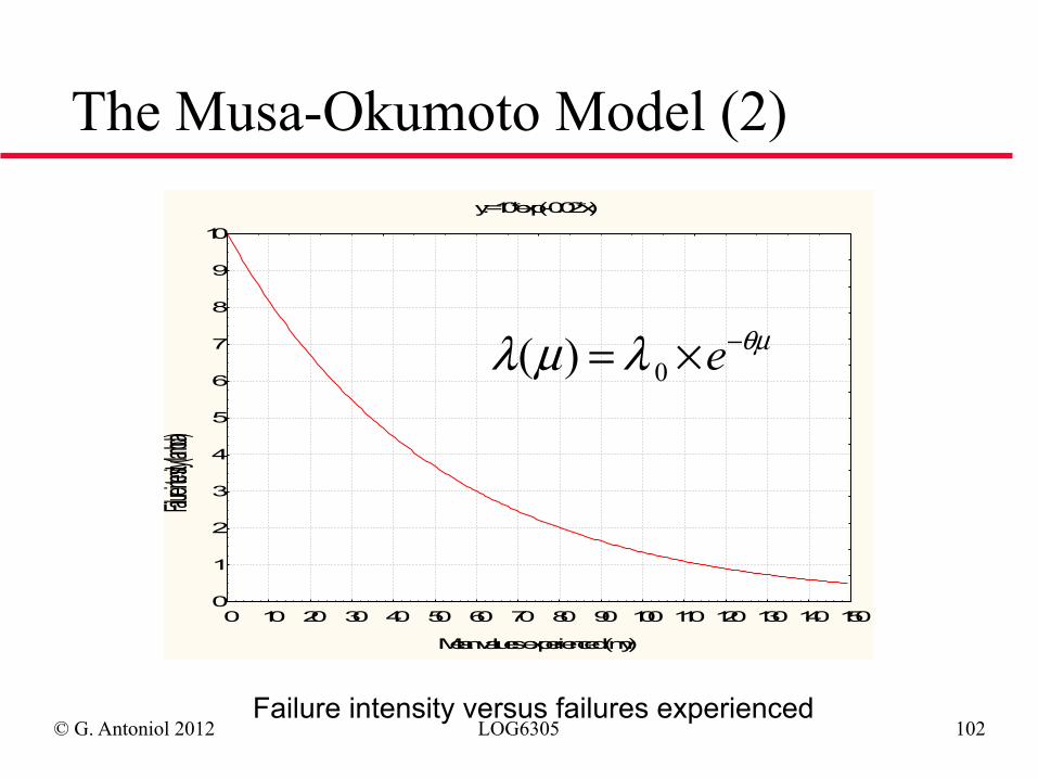
The Musa-Okumoto Model (2)
Failure intensity versus failures experienced
θµλµλ −×= e0)(
y:=10*exp(-0.02*x)
Mean values experienced (my)
Failure intensit
y (lambda)
0
1
2
3
4
5
6
7
8
9
10
0 10 20 30 40 50 60 70 80 90 100 110 120 130 140 150
θµλµλ −×= e0)(
© G. Antoniol 2012 LOG6305 103
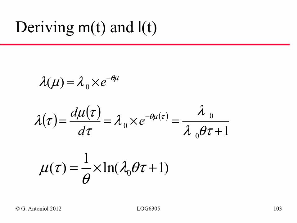
Deriving m(t) and l(t)
θµλµλ −×= e0)(
( ) ( ) ( )10
00 +
=×== −
θτλλ
λττµτλ τθµe
dd
)1ln(1)( 0 +×= θτλθ
τµ
© G. Antoniol 2012 LOG6305 104
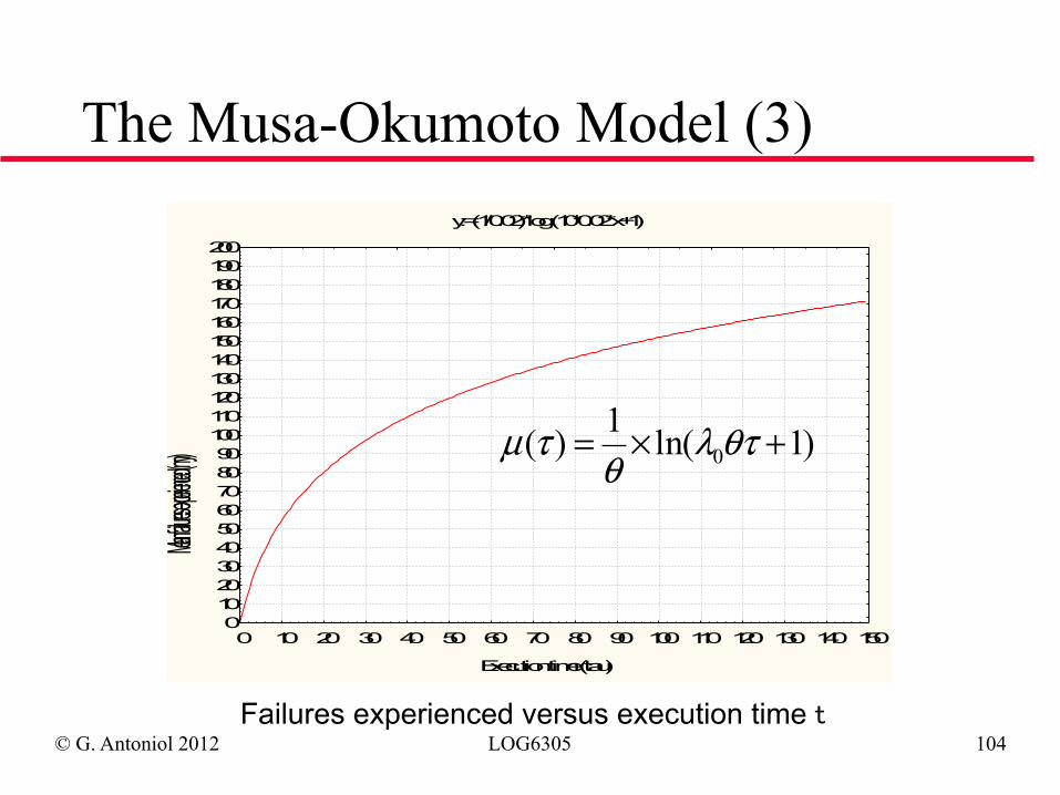
The Musa-Okumoto Model (3) y:=(1/0.02)*log (10*0.02*x+1)
Execution time (tau)
Mean failures
experienced (m
y)
0102030405060708090100110120130140150160170180190200
0 10 20 30 40 50 60 70 80 90 100 110 120 130 140 150
Failures experienced versus execution time t
)1ln(1)( 0 +×= θτλθ
τµ
© G. Antoniol 2012 LOG6305 105
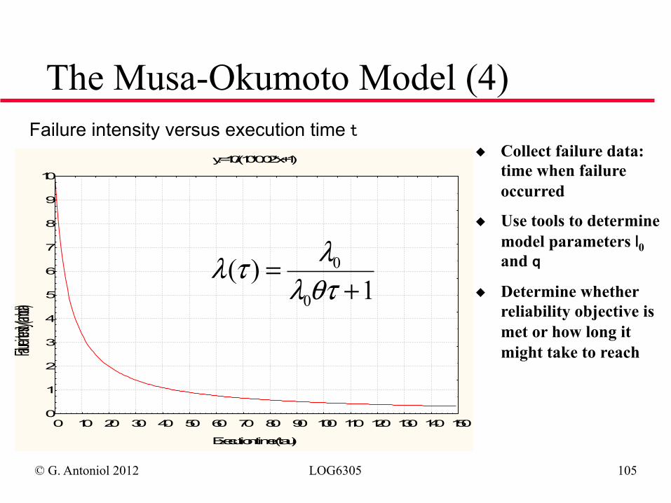
y:=10/(10*0.02*x+1)
Execution time (tau)
Failure intensit
y (lambda)
0
1
2
3
4
5
6
7
8
9
10
0 10 20 30 40 50 60 70 80 90 100 110 120 130 140 150
Failure intensity versus execution time t◆ Collect failure data:
time when failure occurred
◆ Use tools to determine model parameters l0 and q
◆ Determine whether reliability objective is met or how long it might take to reach
The Musa-Okumoto Model (4)
1)(
0
0
+=
θτλλτλ
© G. Antoniol 2012 LOG6305 106
The Musa-Okumoto Model (5)
◆ Once the parameters l0 and � are estimated, it can be used to predict failure intensity in the future, not only to estimate its current value. From this, we can plan how much additional testing is likely to be needed
◆ The model allows for the realistic situation where fault correction is not perfect (infinite number of failures at infinite time)
◆ When faults stop being corrected, the model reduces to a homogeneous Poisson process with failure intensity l as the parameter – the number of failures expected in a time interval then follows a Poisson distribution
© G. Antoniol 2012 LOG6305 107
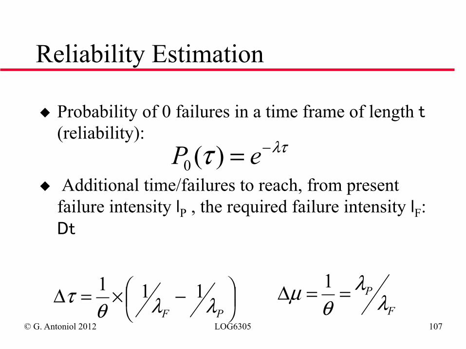
Reliability Estimation
◆ Probability of 0 failures in a time frame of length t (reliability):
◆ Additional time/failures to reach, from present failure intensity lP , the required failure intensity lF: Dt
λττ −= eP )(0
⎟⎠⎞⎜⎝
⎛ −×=ΔPF λλθ
τ 111F
Pλ
λθ
µ ==Δ 1
© G. Antoniol 2012 LOG6305 108
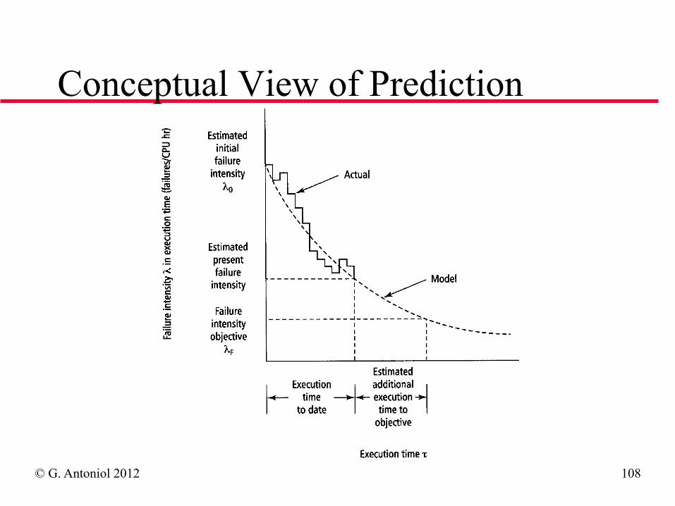
Conceptual View of Prediction
© G. Antoniol 2012 LOG6305 109
Time Measurement
◆ Execution (CPU) time: may be difficult to collect but accurate
◆ Calendar time: Easy to collect but makes numerous assumptions (equivalent testing intensity with time periods)
◆ Testing effort: Same as calendar time, but easier to verify the assumptions
◆ Specific time measurement may often be devised: #Calls, Lines of code compiled, #transactions
© G. Antoniol 2012 LOG6305 110
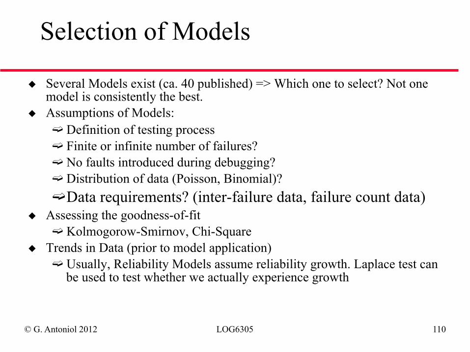
Selection of Models
◆ Several Models exist (ca. 40 published) => Which one to select? Not one model is consistently the best.
◆ Assumptions of Models: ➫ Definition of testing process ➫ Finite or infinite number of failures? ➫ No faults introduced during debugging? ➫ Distribution of data (Poisson, Binomial)? ➫ Data requirements? (inter-failure data, failure count data)
◆ Assessing the goodness-of-fit ➫ Kolmogorow-Smirnov, Chi-Square
◆ Trends in Data (prior to model application) ➫ Usually, Reliability Models assume reliability growth. Laplace test can
be used to test whether we actually experience growth
© G. Antoniol 2012 LOG6305 111
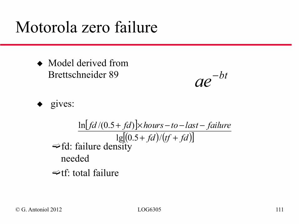
Motorola zero failure
◆ Model derived from Brettschneider 89
◆ gives:
➫ fd: failure density needed
➫ tf: total failure
btae−
[ ]( ) ( )[ ]fdtffd
failurelasttohoursfdfd++
−−−×+/5.0lg
)5.0/(ln
© G. Antoniol 2012 LOG6305 112
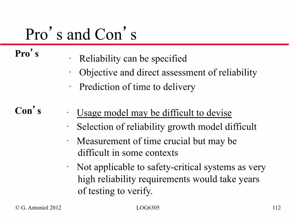
Pro’s and Con’s Pro’s Con’s · Usage model may be difficult to devise
· Selection of reliability growth model difficult · Measurement of time crucial but may be
difficult in some contexts · Not applicable to safety-critical systems as very
high reliability requirements would take years of testing to verify.
· Reliability can be specified · Objective and direct assessment of reliability · Prediction of time to delivery