15IEEE TRANSACTIONS ON SOFTWARE ENGINEERING, VOL. SE-ll, NO. 12, DECEMBER 1985

Assessing (Software) Reliability Growth Using a

Random Coefficient Autoregressive Process

and Its RamificationsNOZER D. SINGPURWALLA AND REFIK SOYER

Abstract-In this paper we motivate a random coefficient autore-gressive process of order 1 for describing reliability growth or decay.We introduce several ramifications of this process, some of which re-duce it to a Kalman Filter model. We illustrate the usefulness of ourapproach by applying these processes to some real life data on softwarefailures. Finally, we make a pairwise comparison of the models in termsof the ratio of likelihoods of their predictive distributions, and identifythe "best" model.

Index Terms-Dynamic linear and nonlinear models, Kalman Filter-ing, likelihood ratios, predictive distributions, prequential analysis,random coefficient autoregressive processes, reliability growth, soft-ware reliability.

I. INTRODUCTION AND OVERVIEW

A COMPLEX newly developed system, such as a pieceof software, undergoes several stages of testing be-

fore it is put into operation. After each stage of testing,corrections and modifications are made to the system, withthe hope of increasing its reliability. This procedure istermed reliability growth.

It is important to recognize that a particular modifica-tion, or series of modifications, could lead to a deterio-ration in performance of the system even though the intentof the modifications is to improve performance. A key is-sue is how to model and how to describe the changes inthe performance of the system as a result of the modifi-cations. The final goal is to be able to predict the behaviorof the system after the last modification, so that a decisionmaker can either continue the test-modify cycle, or ter-minate it, and put the system into final operation.To introduce some notation, let 1, 2, - - *, t denote the

various stages of testing, where the testing at a particularstage follows a modification to the system at that stage.Let X, denote the life length of the system at the tth stageof testing. Having observed X, we would like to be able to

1) determine whether the latest modification, i.e., theone at stage t, has been beneficial;

2) determine whether our policy of deciding upon the

Manuscript received March 3, 1985; revised August 27, 1985. This workwas supported by the Office of Naval Research under Contract N00014-85-K-0202 and by the U.S. Army Research Office under Grant DAAG 29-84-K-0160.

The authors are with the Institute for Reliability and Risk Analysis,School of Engineering and Applied Science, George Washington Univer-sity, Washington, DC 20006.

nature of the modifications and implementing them hasbeen such that there is an overall growth (or decay) inreliability; and

3) make uncertainty statements about X, + 1, the lifelength of the system after the next modification (i.e., ob-tain the predictive distribution of X, + 1).

In addressing the above issues it seems reasonable thatwe take into consideration all the knowledge that we haveabout the system, both due to the physical nature of themodifications and the results of all the previous tests. Fur-thermore, it is reasonable to expect that the life length atthe tth stage is related to the life length at the previousstage(s), unless of course the modifications at the tth stageare of a nature which is drastic enough to change the con-figuration of the system.

In recognition of the above features, Horigome, Soyer,and Singpurwalla [6], henceforth HSS, have viewed thereliability growth process as a time series, and have intro-duced a random coefficient autoregressive process of order1, to describe the series. In this paper, we introduce sev-eral ramifications of the above process, and present themain results for each ramification. An approximation dueto [10] plays a central role in our ability to obtain some ofthe results. We then apply each of the resulting models toa set of software failure data published by [14]. Finally,we make a pairwise comparison of these models in termsof their "prequential properties" [2] using the "likelihoodratios" of [15] and identify that model which appears tobe the best in terms of the above criteria.

II. MOTIVATION FOR THE RANDOM COEFFICIENTAUTOREGRESSIVE PROCESS

Let X, t = 0, 1, 2, * * , denote the time to failure ofthe software after the tth modification is made to it; X0represents the time to failure of the software when it istested for the veryfirst time. It is certainly convenient, butnot unreasonable, to assume that Xt has a lognormal dis-tribution, and that wlog, Xt >- 1, for t = 0, 1, * * *, . Toa subjective Bayesian, this assumption should not be thefocus of a heated debate. Furthermore, the lognormal dis-tribution provides much flexibility in modeling times tofailure of software, for which there is no physical basis foraging. The failure rate of a lognormal distribution can, bya suitable choice of parameters, be made increasing, or

0098-5589/85/1200-1456$01.00 © 1985 IEEE

1456

SINGPURWALLA AND SOYER: ASSESSING SOFTWARE RELIABILITY GROWTH

decreasing, or both increasing and decreasing (see, for ex- by afirst order autoregressive process with a random coef-ample, [4]), the latter feature being relevant for capturing ficient Q. In what follows, we shall focus attention on thethe opinion of an analyst regarding software failures. variables Y, instead of the Xt's.HSS have presented the arguments given below, to ad- First order autoregressive models with random coeffi-

vocate a use of the familiar power law (of, reliability and cients have been considered before in the economics andbiometry) to relate the lifetimes from one stage to the next. statistics literatures, by [1], [11], and [18]. However, theA use of this law enables us to describe the reliability statistical paradigm, and/or the method of analysis consid-growth process. ered by the above authors is different from that considered

Since modifications to the system typically involve mi- by us. The motivation for reliability growth modeling isnor but important changes to its design and configuration, new.it is reasonable to assume that Xt will be related to Xt- l, Having observed Y1 = Yi, Y2 = Y2, . . , Yt = yt, theand it is hoped will be larger than X, - l. Of course, it is prequential view of statistical inference requires us toalso possible that the design changes could be poorly con- make sequential probability forecasts of future observa-ceived so that Xt is equal to Xt - l, or even smaller than tions Y, + l, Yt + 2, * * *, rather than make uncertainty state-Xt- To reflect these features, we write ments about parameters. However, in order to be able to

X a f 11t do this, we must first specify a structure for the stochastic- -I' behavior of the power coefficient Ot.where Ot is a coefficient. Values of at > (<) 1 would de-scribe growth (decay) in reliability. To introduce uncer- A. A Model for Ottainty in our specification of the power law as a model forreliability growth, or to account for the possibility of some We have stated before that it appears reasonable to viewslight deviation from it, either systematic or sudden, we the 0, s as constituting an exchangeable sequence. To fa-introduce a multiplicative error term at, and generalize cilitate our specification of a probability distribution for(2.1) by writing the sequence of Ot's, we recall that all values of O, > 1

imply growth, that 0t = 1 implies neither growth nor de-Xt = Xt-' 1 bt. (2 2) cay, and that all values of Ot < 1 imply decay. When 0, <

Technical convenience demands that we al'so assume bt to 0, the decay in reliability is drastic and is likely to happen2 when the modification is a major design change. The casebe lognormal with known parameters, 0 and 1 . of 0t = 0 is interesting, because from (2.3) we see that YtThe random coefficient feature of our model arises be- = .i

cause of the fact that we allow the coefficient Ot to change et des byYt whes no rmal wt andiS best described by Et, where Et iS normal with mean O andfrom stage to stage. Of the several arguments which jus- 2

tify the changing nature of the coefficient, the most plau- variance arI. When 0t = 0 for all t, (2.3) implies that thesible is that initial modifications to the system are typically sequence { Yt} is a "band limited white noise process" in

the sense of [8, p. 149]. If this were to happen, none ofdue to errors in workmanship and tend to show more im- the previous models for describing reliability growth wouldprovement in reliability than the later ones. Thus the se- be applicable.quence {0t} should be stochastically decreasing in t, withvalues of Ot greater than 1 for small t, and closer to 1 for It icle fothe aboe ta thcoefficis 0canakelarge t. However, this description of 0, may not always be an alue in theranget( oOt+ or) a

T it i reasab' . . . . ~~~~~~toassume that the density of 0, iS normal with a mean, sayoperative, because design alterations, typically dictated by 2an Wh 2S

changes in the system requirements or changes in the po- 'close to u ten tm sa deay i ablity,litical and economic climate, occur at any stage, and could .

cls to.wudtnoepaiz ea nrlaiiyclimat,'oc whereas those in the vicinity of and above would tendmake the system worse. Thus in practice, it may not be t 2

realistic to assign a time pattern to the Ot's. In the contextt mhsz eiblt rwh h auso 2ol

rreflect our views about the consistency of our policies re-of software reliability, for example, the process of cor- g m a d c F' '. ~~~~~~garding modifications and design changes. For example,recting an error at any stage could introduce new errors some design changes could be much more elaborate andmaking the software worse than before. It therefore seems involved than others. When this happens a 2would tend toreasonable to assume a mild form of dependence between bthe Ot's. One way of achieving this is to assume that the be large. If the magnmtudes of the design changes are more

or less of the same order, say all of them are minor, thensequence of 0,'s is exchangeable-but not independent. 2

If we take the natural logarithms on both sides of (2.2), w 2treat 2as being fixed but known.and let E-t = log at, t = l, 2, * * -* then our power lawtra 2sbigfxdutkonandellet 'i='logro,t= 12co ten The usual strategy for ensuring that the 0,'s constitutemodel for reliability growth becomes an exchangeable, but not independent, sequence is to as-

Yt = 0t Yt-1 + t,t (2.3) sume a probability distribution for X as well. This is bestdef done by assuming X to be normal with a known mean ,u

where Y, = log X, and E, are both normally distributed, and a known variance a. Because of our discussion aboutthe latter with mean 0 and variance u . It is clear from the the influence of the possible values of X on the growth orabove that the sequence { Yj}, t = 1, 2, - - *, is described decay of reliability, an innocuous choice for i is 1.0. The

1457

IEEE TRANSACTIONS ON SOFTWARE ENGINEERING, VOL. SE-ll, NO. 12, DECEMBER 1985

value aJ should reflect the strength of our belief about ourchoice of,u.

Thus, to summarize, our model for the growth or decayof reliability, for Y, = log Xt, t = 1, 2, , is of the form

Y= 0,Y,-I + E1, with

et N(O, a2), a2 known,

ot - N(X, C2), OF known, and

X - N(It, o2), It and a3 known. (2.4)

In (2.4) above, Ot is assumed independent of Et. In whatfollows, we shall let y(t) = (Yl, * - *, yt), and given y(rour objective is to make inferences about0T9 X, YT+ 1, andif necessary YT d-f log XT, where XT is the time to failureof another copy of the system.

It is useful to note that E(0, y(t)) gives us informationabout reliability growth or decay from stage (t - 1) tostage t, whereas E(X y(t)) gives us information about theoverall growth or decay in reliability. Thus for example,E(X y(t)) tends to be greater than 1, for most of the valuesof t, especially the large values, we may conclude thatthere is an overall growth in reliability.

In what follows, we shall refer to the model specifiedby (2.4) as Model I. Ramifications of this model, whichemanate from assuming alternate structures for the de-pendence between the Ot's, are discussed in the next sec-tion.

III. SOME RAMIFICATIONS OF THE RANDOM COEFFICIENTAUTOREGRESSIVE PROCESS

An obvious way to extend Model I would be to let (2.3)be an autoregressive process of orderp > 1. However, thisis not the direction that we choose to pursue here, be-cause, to do so would required that (2.1) be extended ast= tI '2* X0tp , a relationship with an intu-

itive and simple motivation. Instead, we propose to staywith (2.3), but impose on the sequence 0t, structures forEdependence which are stronger than that of exchangeabil-ity.A natural model for dependence between the 0,'s is the

first order autoregressive process with the autoregressivecoefficient a known, and for convenience set equal to 1.That is, we let 0O = Ot- I + wt, where the innovation w, isassumed normal with mean 0 and known variance W,. Weshall refer to this set up as Model II, and for conveniencespell it out below as

Yt= O,Yt-I + Et with

et N(O, u2), with or known, and

Ot = Ot-I + wt, with

w, ~N(O, W,), with W, known. (3.1)Note that (3.1) is a special case of an Ordinary Kalman

Filter Model considered by [12]; it is referred to by [5] asthe steady model. Here the Ot's are assumed to be con-stant, except for the random changes brought about by the

innovations w. Inference about the pertinent quantitiesusing this model follows along well established lines ofKalman Filtering.A generalization of (3.1) leads us to Model III, wherein

the 0a's are described by an autoregressive process of order2, with the autoregressive coefficients a, and a2 also as-sumed known. Specifically, this model can be written as

Yt= 01Yt-I + ct, with

(t N(O, a2), with a known, and

0t = to-I + a201-2 + WI, with

w, - N(O, W,), with a1, a2 and WT, known. (3.2)

Since Model III is also a special case of the KalmanFilter model, inference about the pertinent quantities usingthis model proceeds along familiar lines.

In both Model II and Model ILL, we assumed the auto-regressive coefficients for Ot known. Model IV, given be-low, is a generalization of Model II, in the sense that theautoregressive coefficient oa is assumed unknown. Wewrite out this model, in detail, as follows:

Yt= OtY,- + E,, with

(t NN(0, or2), with or known, and

0, = at-I + w,, with

wt ~N(0, W,), with WT, known. (3.3)Since a is unknown, the Bayesian paradigm requires

that we assign a prior distribution for it. A convenient priorfor a is the uniform on [a, b].We refer to model (3.3) above as an Adaptive Kalman

Filter Model. Even though (3.3) is a slight generalizationof the ordinary Kalman Filter Model (3.1), its analysisproduces technical difficulties, in the sense that the auto-matic and closed form nature of the ordinary Kalman Fil-ter is lost. It is here that an approximation due to Lindleyplays an important role. In Model IV we have a type ofextension of the Kalman Filter model which has rarelybeen considered before. Furthermore, our approach to itsanalysis is new and represents a contribution to the liter-ature of Kalman Filtering.

It is to be noted that in (3.2)-(3.4), the innovations E,and wt are assumed independent of each other.

Finally, we would like to remark that there are no con-vincing physical arguments which motivate the need for(3.2)-(3.4), beyond those used for motivating (3.1). Theramifications given in this section are purely technical.Our hope is that these ramifications may lead to improve-ments in the predictive performance of the new models,as compared to that of Model I. Model I, with a generalstructure for dependence between the 0t's from a subjec-tive point of view, is our preferred model.

IV. COMPARISON OF MODELSThe Bayesian paradigm does not enable us to formally

compare more than two models at the same time. Conse-

1458

SINGPURWALLA AND SOYER: ASSESSING SOFTWARE RELIABILITY GROWTH

quently, we will be making pairwise comparisons to seeif any of the four models of this paper appears to dominatethe others in terms of the ratio of likelihoods of observedvalues based on two predictive distributions. An overviewof this approach, due to [15], is given below. Since ModelI is our preferred model, we will be comparing this modelto each of the other three.

Let us suppose that we wish to compare two models,say A and B, based on their predictive distributions forY,+1 given the data Y for t = 1, 2,- ,. Let thesepredictive distributions be denoted by P (Y, + y ( A) andP(Yt+ 1 Yt B), respectively. Let P (A) and P (B) denoteour "prior weights" assigned to models Al and B, respec-tively. These weights reflect our belief in the relative per-formance of the two models prior to any inference and anypredictions using these models. The ratio P (A)IP (B) isthe prior ratio of weights A to B, and in the terminologyused by' Savage is "private" to us. The ratio P(A yP (B |y (t)) represents our posterior ratio of weights A toB, posterior to the' data y(t). It is obtained by multiplyingthe prior ratio of weights by the ratio p (y() A)lp (Y(t) B).The ratio p (t) A)Ip(y(t) B) is a likelihood ratio and inthe terminology of [16], this ratio is fully "public." If wechoose P(A)IP(B) = 1, that is, if a priori we have nopreference of one model over the other, then

P(AIy(t)) P(ytI y(t-) A)

P(BIy)) P(ytl y(t-1), B)

Model IThe posterior distribution of X, given y(t) is

(- y (t)) - N(Mt, St)where

Mt= y , whereSt_Iy2_1 + rt

St- I rtSt= 2 , and

St-lyt-I + rt

r 2= or2y21 + ao; Mo and So a2.The posterior distribution of Ot given y(t) is

(ot y (t) N(Ot, ASt)where

A 2lMt + y2Yt Yt_ Iot= M and

rt

2(u2S, + or2)AnohI trn

(5.1)

(5.2)

And the predictive distribution of Y, given y t- I) is alsoa normal:

* (Yt I Y(t- I)) - N(Mt Ilyt- (, y52_(5.3)

P(yt-l Y(t-2) A)p( IIy(t-2) B)

P(yI IA)P(y1 B)

where Yi,Y2l, , y, are the observed values of Y1,Y2,, Y,. Note that the ratio' P(y, y(t-l), A)!P (yt y -), B), is a ratio of the likelihood of yt, givenY(t-l), under A and B. The likelihood P(ytI y(-), A) isobtained by replacing Y, by its observed value y, inP(Y,I y(t- 1), A), the predictive distribution of Yt givenY(-1) under model A.

If the posterior'ratio of weights A to B is greater than1, then model A is to be preferred over model B; otherwisethe reverse is true.

In Section VI, we shall compare Model I versus Model= II, III, and IV, using the posterior ratio of weights

A to B given above.

V. MAIN RESULTS ON INFERENCE

The emphasis of this paper is a motivation for the ran-dom coefficient autoregressive process (2.4) as a model forreliability growth, and a comparison of this model to itsramifications-'when applie'd to some data on software re-liability. The details regarding the development of the nec-essary results of infeience are given in [17]. What wepresent below is'merely a statement of the key results foreach model.

Model IIThe key results for Model II are obtained via Kalman

Filter solution [121.The posterior distribution of 0, given y ( is

(Ot Y Nt) (oNt, St) (5.4)where

=Ot_ I or + Rtytyt-t Yt2_Rt + Or2

A Rt or

Yt _1Rt + r2'

t= St-1 + Wt

The predictive distribution of Yt given y t- ') iS

(5.5)

Model III

Model III is a special case of the Kalman Filter model.Thus, the main results can be obtained via Kalman Filtersolution.The posterior distribution of 6, given y ' is

(5.6)

where

1459

(t 1) A 2 2).(Yt y ) - N(yt-lot-1, yt _,Rt + orl

. (Ot Y (1)) - N (O', E't)

IEEE TRANSACTIONS ON SOFTWARE ENGINEERING, VOL. SE-lb, NO. 12, DECEMBER 1985

a= I(Ot lI + 2Ot- 2) I+ Rtytyt_Rt+ Ul

RtOFt 2 +r2 andYt _j-Rt + I2

Rt = I Et-I + °x2Et-2 + 2a10a2-t-1,t-2 + Wtwhere

=coy~~~~ 0~~21y~(tI)Et- 1,t-2 =COV (Ot- 1, Ot-21 Y( )

The covariance Et,t-I can be computed by using the re-cursion

=tt 1 (a 1 1 2 t 1, t 2 ) t t (5.7)The predictive distribution of Yt given y(t- 1)is

(Yy(t- 1)) N[Yt-1 (U IOt -1 + a2,t-2)

Y,1Rt + or,] (5.8)

Model IVModel IV, which we have referred to as an Adaptive

Kalman Filter, is a generalization of the ordinary KalmanFilter model. There are no closed form solutions for theposterior distribution of Ot given y(t) and the predictive dis-tribution of Yt given y(t - 1), Thus, we use an approximationby [10] to compute these distributions.The posterior distribution of Q given y(t) can be approx-

imated by the expansion

2+ 2P HI +P (.9p(Qty(l), &) {1 - 2L2 + 2L2 (5.9)

where p(Otly(t), a) denotes the probability density of Otgiven y(t) and a, with

P = loge [P (ItY &)],L = loge [p((t) &)] - log likelihood of a,

H = loge [p(&lJC)] - log of the prior for a, and

Pi, Li, and Hi are the ith derivatives of the correspondingfunctions with respect to a. All the functions and theirderivatives are evaluated at &^, the maximum likelihoodestimate of a.We note that p (OtI y(t), a) is the posterior density of 0,

when oa is known and can be obtained from ordinary Kal-man Filter solution. We obtain the predictive distributionof Yt given y(i-I), by using the same expansion withp(yy(t-l) a) replacing p (Ot Iy(t), ') in (5.9).We can compute the posterior mean and other posterior

moments of Ot by using a similar expansion

_(t A E2 + 2E1H1 El L3E(Ot E(t Iy(t, a I-

2L2E + 2L~E)

where

E = E(t yy,&)

and

a 'EE(0OtI Y, a)au1 i = 1, 2.

Similarly, we obtain the predictive mean of Y, given y(t - 1)with E(YtIy(t-1), ) replacing E(0 y(t, 'a) in (5. 10). Thedetails for developing the necessary formulae for inferenceare given in [17].

VI. APPLICATION OF THE MODELS TO MUSA'S DATA ON

COMPUTER SOFTWARE FAILURESMusa [14] has published several sets of data on the fail-

ure times of computer software which undergoes a debug-ging process. We shall apply the four models introducedin Section III to the data set of [14] labeled as "'System 40data." We do this for illustrative purposes only, to see howModel I and its ramifications perform on software failuredata and to see what insights about reliability growth wecan obtain from our analysis. We present the results in theAppendix.

In Appendix A, column 2, we present values of Y, =loge Xt, t 0, 1, * * *, 100, where X, are the executiontimes given by Musa. In columns 3, 4, 5, and 6 we presentthe values of Yt, the means of the predictive distributionsof Y, for Models I, II, III, and IV, respectively.

In undertaking the computations which lead us to theresults presented in Appendixes A and B, we choose thestarting values in each model as follows:

In Model I: Ir = 1.0, u2= 1.0, u2 = 0.25 and t -1.0.

In Model II: a2 = 1.0, W, 1.0 for all t, 00 = 1.0 andEo = 0.25.

In Model III: o2 = 1.0, WV = 1.0 for all t, a1 = 0.5, Z2= 0.5, 00 = 1.0, 01 = 1.0, Eo = 0.25, El = 0.25, and El0= 0.0.In Model IV: u1 = 1.0, W, = 1.0 for all t, 00 = 1.0, E0

= 0.25 and the parameters of the prior density of ae are a= -2.0 and b = 2.0.Given the large amount of data, our final conclusions

are not too sensitive to the choice of these values; the ex-ception is a1 and a2 of Model III.We are not able to judge the predictive performance of

these models merely based on the results presented in Ap-pendix A, but a comparison of column 2 with columns 3,4, 5, and 6 shows that these models perform reasonablywell for predicting the (logarithms of) the next executiontimes.As stated in Section II, the value E(0,1 y(t)) gives us in-

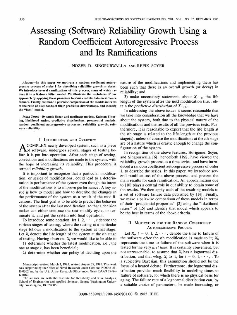
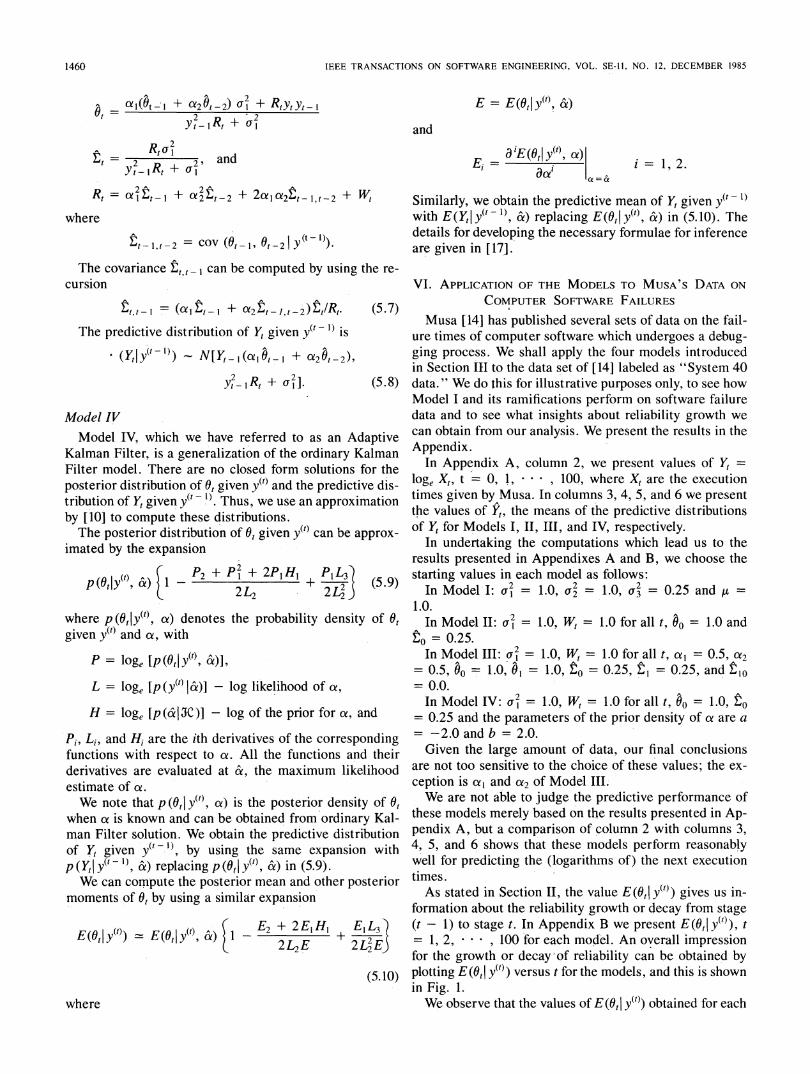
formation'about the reliability growth or decay from stage(t - 1) to stage t. In Appendix B we present E(0t Iy()), t= 1, 2, * * , 100 for each model. An overall impressionfor the growth or decay- of reliability can be obtained byplotting E(0,I y(t)) versus t for the models, and this is shownin Fig. 1.We observe that the values of E(0,1 y(t)) obtained for each

1460

SINGPURWALLA AND SOYER: ASSESSING SOFTWARE RELIABILITY GROWTH

ett029

Ot

AD 40 1000Q7Qs l'o 20 a

(a)

1 ~~~~~~~~~~~~~~~~E(Ot{Y)

III,~~~~~~~~~~~~~~~~~~~~~~~~~~~ (dMoel.V

7

,2

aI0~~~~~~~~~~~~~~~~j

(b)Fig. 1. Posterior means of 0, using (a) Model I, (b) Model II, (c) Model

III, (d) Model IV.

E( (t )

1i s0 u t

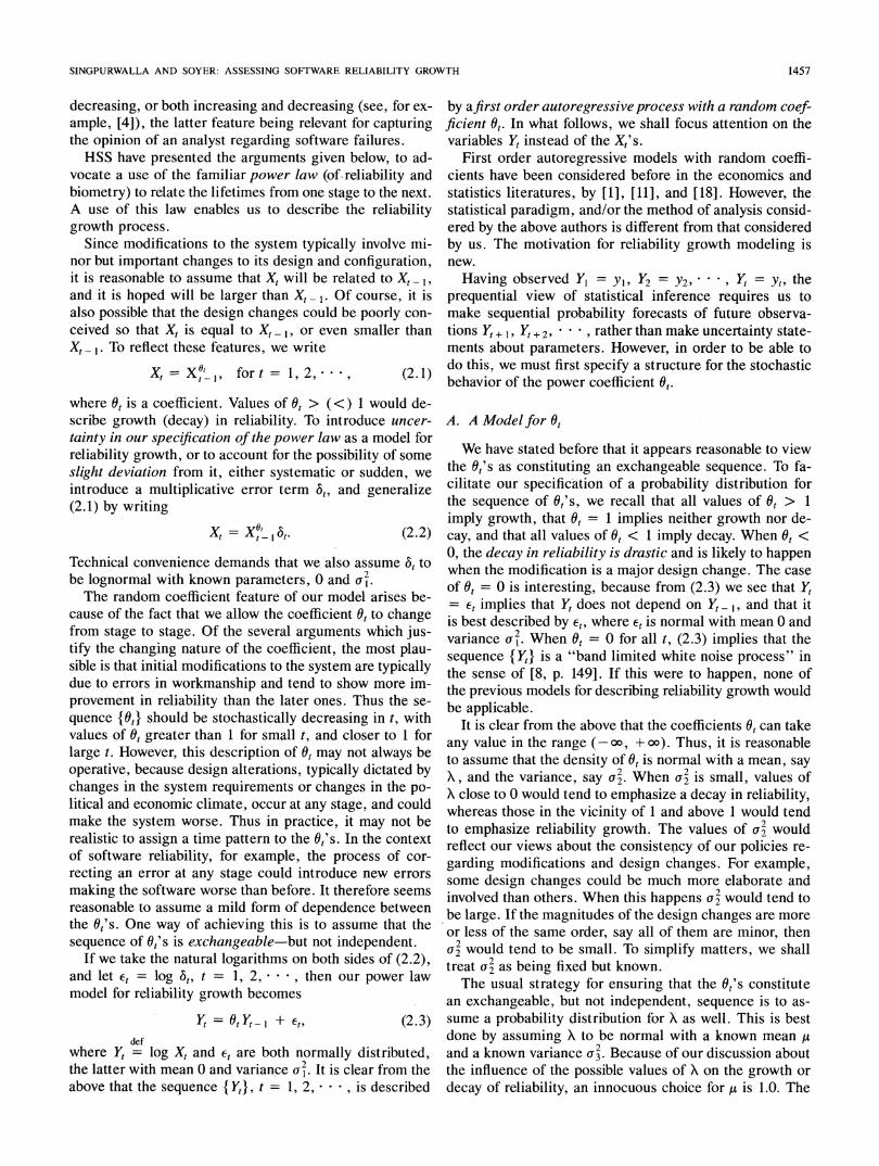
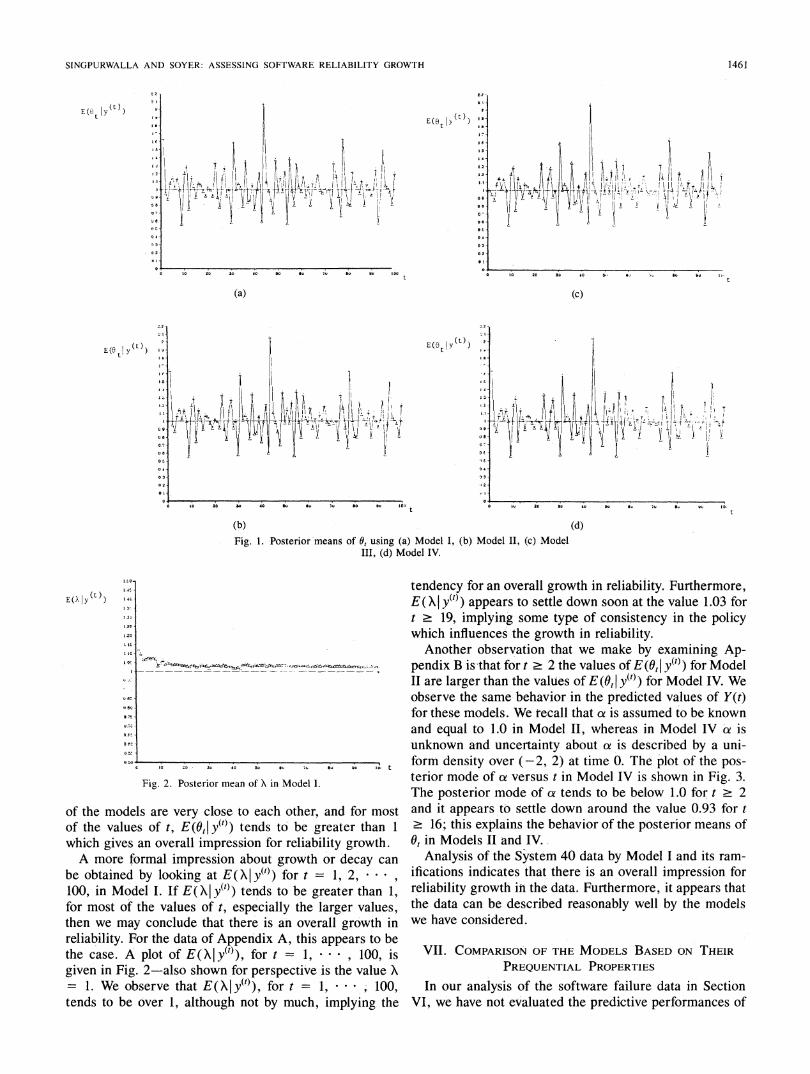
Fig. 2. Posterior mean of X in Model l.

of the models are very close to each other, and for mostof the values of t, E(OtI y(t)) tends to be greater than 1

which gives an overall impression for reliability growth.A more formal impression about growth or decay can

be obtained by looking at E( XIy(')) for t = 1, 2, * * *100, in Model I. If E( XI Y(0)) tends to be greater than 1,for most of the values of t, especially the larger values,then we may conclude that there is an overall growth inreliability. For the data of Appendix A, this appears to bethe case. A plot of E(XIy(0t), for t = 1, , 100, isgiven in Fig. 2-also shown for perspective is the value X= 1. We observe that E(XIy(t)), for t = 1, * * *, 100,tends to be over 1, although not by much, implying the

tendency for an overall growth in reliability. Furthermore,E (X y(t)) appears to settle down soon at the value 1.03 fort > 19, implying some type of consistency in the policywhich influences the growth in reliability.

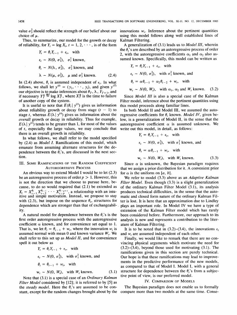
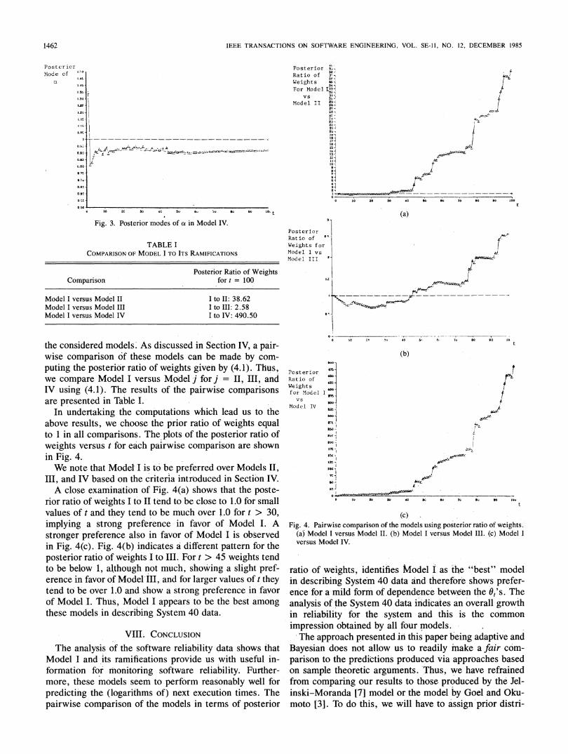
Another observation that we make by examining Ap-pendix B is that for t 2 2 the values of E(OtI y(t)) for ModelII are larger than the values of E (t I y(t)) for Model IV. Weobserve the same behavior in the predicted values of Y(t)for these models. We recall that ca is assumed to be knownand equal to 1.0 in Model II, whereas in Model IV 'e isunknown and uncertainty about ae is described by a uni-form density over (-2, 2) at time 0. The plot of the pos-terior mode of a versus t in Model IV is shown in Fig. 3.The posterior mode of at tends to be below 1.0 for t 2 2and it appears to settle down around the value 0.93 for t> 16; this explains the behavior of the posterior means ofOt in Models II and IV.

Analysis of the System 40 data by Model I and its ram-

ifications indicates that there is an overall impression forreliability growth in the data. Furthermore, it appears thatthe data can be described reasonably well by the modelswe have considered.

VII. COMPARISON OF THE MODELS BASED ON THEIRPREQUENTIAL PROPERTIES

In our analysis of the software failure data in SectionVI, we have not evaluated the predictive performances of

E t|Y )

EE(6tI

(c)

(d)

1461

[.'.O-

1.41-

IAG

.3 1.

1,3.1

Lk,

-20

i it

10

I ol-

I--

1 2

f, a .1-

" a,,

0.71-

u.7C

O.ft -

a (IC

0 -V

0 5.0 I

ze--Intl-e

IEEE TRANSACTIONS ON SOFTWARE ENGINEERING, VOL. SE-11, NO. 12, DECEMBER 1985

Posterior s,-Ratio of 31

Ratio~~~~~~~~~~~~~~~~~~~aWeights 1|For Model T133

Vs 3'-

Model II t9

27-10..

Is313.i915

6

6 0t

o l0 ac 30 10 5U ;0 t

Fig. 3. Posterior modes of a in Model IV.

TABLE ICOMPARISON OF MODEL I TO ITS RAMIFICATIONS

Posterior Ratio of WeightsComparison for t = 100

Model I versus Model II I to II: 38.62Model I versus Model III I to III: 2.58Model I versus Model IV I to IV: 490.50

the considered models'. As discussed in Section IV, a pair-

wise comparison of these models can be made by com-

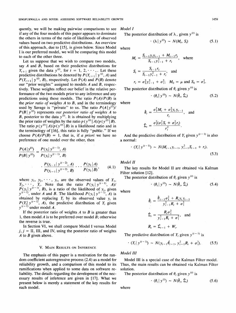
puting the posterior ratio of weights given by (4.1). Thus,we compare Model I versus Mpdel j for j =II, III, andIV using (4.1). The results of the pairwise comparisonsare presented in Table I.

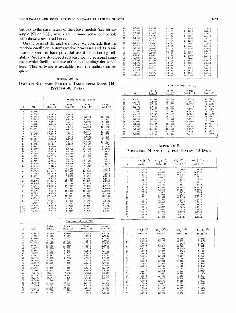
In undertaking the computations which lead us to theabove results, we choose the prior ratio of weights equalto 1 in all comparisons. The plots of the posterior ratio ofweights versus t for each pairwise comparison are shownin Fig. 4.We note that Model I is to be preferred over Models II,

III, and IV based on the criteria introduced in Section IV.A close examination of Fig. 4(a) shows that the poste-

rior ratio of weights I to II tend to be close to 1.0 for smallvalues of t and they tend to be much over 1.0 for t > 30,implying a strong preference in favor of Model I. Astronger preference also in favor of Model I is observedin Fig. 4(c). Fig. 4(b) indicates a different pattern for theposterior ratio of weights I to III. For t > 45 weights tendto be below 1, although not much, showing a slight pref-erence in favor of Model'III, and for larger values of t theytend to be over 1.0 and show a strong preference in favorof Model I. Thus, Model I appears to be the best amongthese models in describing System 40 data.

VIII. CONCLUSIONThe analysis of the software reliability data shows that

Model I and its ramifications provide us with useful in-formation for monitoring software reliability. Further-more, these models seem to perform reasonably well forpredicting the (logarithms of) next execution times. Thepairwise comparison of the models in terms of posterior

PosteriorRatio ofWeights forModel I vs

Model III

O 10 20 to o0 Oo u1 7 ~ o De loo

(a)

.T

fh=w1

d

dt/~~~~~~~~~~~~~~~~~~~~~~~

a so ^rI .w 40 5* FI #9 so 9 ((

(b)

Post erisorRatio ofWeight s

for Modelvs

Model IV

I o?5I.o I

2

Llso -

toto -I7

17.i -

t

it

.t

(c)

Fig. 4. Pairwise comparison of the models using posterior ratio of weights.(a) Model I versus Model II. (b) Model I versus Model III. (c) Model Iversus Model IV.

ratio of weights, identifies Model I as the "best" modelin describing Syste'm 40 data and therefore shows prefer-ence for a mild form of dependence between the 0 's. Theanalysis of the System 40 data indicates an overall growthin reliability for the system and this is the common

impression obtained by all four models.The approach presented in this paper being adaptive and

Bayesian does not allow us to readily make a fair com-

parison to the predictions produced via approaches basedon sample theoretic arguments. Thus, we have refrainedfrom comparing our results to those produced by the Jel-inski-Moranda [7] model or the model by Goel and Oku-moto [3]. To do this, we will have to assign prior distri-

Pos ter iorMXode of '"' °

1.4c

I1.40

1I3.:1

.30

&

wtO

IG

L .

Qt.S;

a.90

ozs

0.eog.r.

tG.-, v

0.61.

O0.6D

G '-'

1462

t

475

.-

uZ

SINGPURWALLA AND SOYER: ASSESSING SOFTWARE RELIABILITY GROWTH

butions to the parameters of the above models (see for ex-

ample [9] or [13]), which are in some sense compatiblewith those considered here.On the basis of the analysis made, we conclude that the

random coefficient autoregressive processes and its rami-fications seem to have potential use for monitoring reli-ability. We have developed software for the personal com-

puter which facilitates a use of the methodology developedhere. This software is available from the authors on re-

quest.

APPENDIX ADATA ON SOFTWARE FAILURES TAKEN FROM MUSA [14]

(SYSTEM 40 DATA)

Using Using Using Usingt Y(t) Model I Model II Model III Model IV

0 5.7683 - -

1 9.5743 5.7683 5.76832 9.1050 10.8081 15.74323 7.9655 10.0095 8.72194 8.6482 8.5025 6.97645 9.9887 9.2509 9.36166 10.1962 10.7791 11.52767 11.6399 10.9435 10.42138 11.6275 12.5653 13.27499 6.4922 12.4737 11.6271

10 7.9010 6.7074 3.645811 10.2679 8.2653 9.496312 7.6839 10.9138 13.328413 8.8905 8.0161 5.789314 9.2933 9.3340 10.227415 8.3499 9.7545 9.726416 9.0431 8.6979 7.516317 9.6027 9.4386 9.770718 9.3736 10.0310 10.199119 8.5869 9.7625 9.158520 8.7877 8.8964 7.872121 8.7794 9.0998 8.980822 8.0469 9.0784 8.773623 10.8459 8.2847 7.383924 9.7416 11.2937 14.548425 7.5443 10.0939 8.785626 8.5941 7.7489 5.852627 11.0399 8.8592 9.736628 10.1196 11.4706 14.159829 10.1786 10.4756 9.305830 5.8944 10.5276 10.229531 9.5460 6.0174 3.437232 9.6197 9.9059 15.185533 10.3852 9.9743 9.753234 10.6301 10.7800 11.204435 8.3333 11.0302 10.886136 11.3150 8.5926 6.550237 9.4871 11.7592 15.272538 8.1391 9.8129 7.991639 8.6713 8.3844 6.981340 6.4615 8.9398 9.2118

9.57438.38407. 27808.471211.166811.085612. 587412.44505.06916.988612.83537.86098.4807

10. 21808.12008.962810.28709.55268. 13348.52238.87 197.7107

12. 254510.92086.33018.216113.326711.12769.80044. 6845

10.402212. 530910.8 55211.19197.541812.094110. 39636. 92128. 3362

31.46917. 29855. 90058.402410.64489.525412.418910.77373. 25758.802412.55375. 20749.43308. 95036.88269.06249.48518.50667.31078. 39768.21516.9043

13.85078.19865.44739.167413.43898.71649. 62133. 1938

14. 38909.0268

10.412510.12036.059214.31357. 37836. 45588. 5647

I3~~~~~~~~~~~~~~~

Predicted value of Y(t)

Using Using Using UsingY(t) Model I Model 11 Model III Model IV

41 6. 461542 7.695543 4.700544 10.002445 11.012946 10.862147 9.437248 6. 664449 9. 229450 8.967151 10. 353452 10.099853 12.607854 7 .1 54655 10.003356 9.860157 7.867558 10.575759 10. 929460 10.660461 12.497262 11. 374563 11. 915864 9 .575065 10.4504

6.6196 4.84146.6162 6.42418.1919 9.77614.7904 2.819210.4177 20.632411.4835 12.226011.3140 10.72439.7977 8.20856.8764 4.71839.5838 12.64559.3004 8.7528

10.7603 11.931610.4852 9.868713.1355 15.70577.3952 4.0901

10.4011 13.828810.2433 9.75698.1421 6.2928

10.9974 14.125511.3641 11.323711.0736 10.403313.0074 14.629211.8162 10.371312.3801 12.47059.9147 7.7102

5.84835. 64028. 85084. 283313.374617. 508111. 37498. 78325. 26149.6011

10.510711.011810.761914. 01286. 50149. 801811.70647.0314

11.310512. 956310.718313.421811.841211. 6690

4.47095.96349.13432. 5915

19.388111. 09049.72747.44024. 2686

11. 55897.937710.87628.979514.38213. 6967

12.61378.83705.6897

12.878310.27979.4502

13.34689.4337

11.37768.8680 7.0159

66 10.586667 12.720168 12. 598269 12.085970 12.276671 11.960272 12.024673 9.287374 12.495075 14. 556976 1 3. 32 7977 8.946478 14.782479 14.896980 12.139981 9.798182 12.090783 13. 097 784 13.368085 12.7 206

10.8297 11.373810.9673 10.731713.2073 15.262613.0723 12.493512.5277 11.596912.7219 12.465712.3840 11.655212.4459 12.08689.5809 7.1879

12.9403 16.729315.0996 16.975013.8044 12.21829.2257 6.011815.3558 24.247715.4692 15.054712.5737 9.903810.1218 7.908612.5184 14.866913.5683 14.201513.8459 13.6488

9.898811. 127014.072613.803411.791612.127411.899411.90218.2618

13. 207518.229113. 87097.1144

17.111519. 74011 1. 08147. 9609

12.317215.144314. 0649

10.39379. 8073

14.004011.440810.627011.442710.703611.11516.5952

1 5.44971 5. 655011. 24195. 5249

22.457213.80099.06747. 244 0

13. 680313.056912.5528

APPENDIX BPOSTERIOR MEANS OF et FOR SYSTEM 40 DATA

E( tly( )) E(ytty ) E( tly( E( t1y(t)

t Model I Model II Model III Model IV

1 1.6443 1.6443 1.0000 1.65782 0.9526 0.9583 0.9515 0.95503 0.8771 0.8758 0.8759 0.87414 1.0855 1.0825 1.0831 1.08115 1.1540 1.1541 1.1528 1.15296 1.021-3 1.0221 1.0217 1.02117 1.1410 1.1405 1.1411 1.13988 0.9995 0.9999 0.9995 0.99939 0.5618 0.5616 0.5621 0.5608

10 1.2130 1.2019 1.2070 1.200911 1.2958 1.2981 1.2931 1.296912 0.7511 0.7534 0.7530 0.752213 1.1552 1.1504 1.1548 1.149414 1.0454 1.0466 1.0442 1.045515 0.9001 0.9002 0.9008 0.899216 1.0825 1.0805 1.0815 1.079517 1.0617 1.0621 1.0610 1.061218 0.9768 0.9771 0.9772 0.976219 0.9174 0.9168 0.9172 0.916020 1.0235 1.0220) 1.0224 1.0212

E(to ly Moel It) E(Mo ly II) E(Mtoly )

t Model I Model II_ Model III Model IV

21 0.999522 0. 918023 1.343224 0.899325 0.7777126 1.137327 1.281328 0.917629 1.006130 0.583331 1.603232 1.008033 1.079134 1.023735 0. 786136 1.353337 0.840038 0.859839 1.064940 0.748841 1.000642 1.228043 0.5968

0. 99930.91761. 34140.90190. 77581.13291.28260. 91961.00500.58311.59081.01391.07891.02410.78601. 34980.84240. 85771.06230. 74930. 99421. 22730.5998

0. 99870.91781.34200. 90010. 77801. 13401. 28030. 91901.00670.58271.59671.00861.08191.02380. 78631.35140.84020.86051.06220. 74800. 99781. 22450. 5980

0. 99850.91681.39070. 90110. 7 7511.13221.28180. 91891.00450. 58231.58991.01261. 07811.02340. 78541. 34910.84160.85711.06140.74820. 99301.22580.5983

1463

Predicted value of Y(t)

Predicted value of Y(t)

Using Using Using Usingt Y(t) Model I Model II Model III Model IV

86 14.1920 13.1633 12.1094 12.5523 11.138287 11.3704 14.6987 15.8194 14.6675 14.587588 12.2021 11.7469 9.1273 10.8997 8.391889 12.2793 12.6114 13.0694 11.4370 12.051990 11.3667 12.6876 12.3623 12.7591 11.400391 11.3923 11.7316 10.5280 10.9819 9.707892 14.4113 11.7545 11.4113 10.9845 10.537093 8.3333 14.9045 18.2015 16.3186 16.866794 8.0709 8.5791 4.8458 7.6817 4.454595 12.2021 8.3040 7.7726 6.2499 7.164096 12.7831 12.6137 18.3481 15.0614 16.011197 13.1585 13.2161 13.4301 16.2962 12.386198 12.7530 13.6036 13.5466 13.6828 12.503399 10.3533 13.1763 12.3644 12.7557 11.4137

100 12.4897 10.6746 8.4151 9.2267 7.7609

IEEE TRANSACTIONS ON SOFTWARE ENGINEERING, VOL. SE-It, NO. 12, DECEMBER 1985

44 2.080945 1.100446 0.986847 0.870248 0. 709849 1.377350 0.972351 1.153252 0.9761

53 1.246354 0. 570455 1.391356 0.986257 0.800358 1.339459 1.033560 0.975961 1.171262 0.911063 1.047564 0.805265 1.0908

2. 06271. 11020.987 30. 86980.7 0791.37010. 97611. 15240.97711. 24 570.57181.38240.98950.79981.33571.03610.97591.17060. 91181. 04 660. 80521.0884

2.07631.10330. 99110. 8 7030.70871.37190. 97 241. 15480. 97631.24660.57081.38890.98560.80181. 33711,03380. 97 711.17090. 91121 .04760. 80481.089 7

2.06111.10840.98650.86900.70711. 36880. 9 7471.15140. 97621. 24490.57091.38150. 98830.79891.33451. 03500.97511 .16990. 91111.04590.804 61.0876

ACKNOWLEDGMENT

We would like to express our appreciation to Prof. P. K.Goel for suggesting one of the ramifications considered inthis paper.

REFERENCES

[I] T. W. Anderson, "Repeated measurements on autoregressive pro-cesses, J. Amer. Statist. Ass., vol. 73, pp. 371-378, 1978.

[2] A. P. Dawid, "Statistical theory: The prequential approach," J. Roy.Statist. Soc., part A, vol. 147, pp. 278-292, 1984.

[3] A. L. Goel and K. Okumoto, "Time-dependent error-detection ratemodel for software reliability and other performance measures," IEEETrans. Rel., vol. R-28, pp. 206-211, 1979.

[4] L. R. Goldthwaite, "Failure rate study for the lognormal lifetimemodel," in Proc. 7th Nat. Symp. Rel. and Quality Contr., 1961, pp.

208-213.

[5] P. J. Harrison and C. F. Stevens, "Bayesian forecasting (with discus-sion)," J. Roy. Statist. Soc., part B, vol. 38, pp. 205-247, 1976.

[6] M. Horigome, N. D. Singpurwalla, and R. Soyer, "A Bayes empiricalBayes approach for (software) reliability growth," in Proc. 16th Com-put. Sci. Statist. Symp. Interface, L. Billard, Ed., 1984, pp. 47-56,1984.

[7] Z. Jelinski and P. B Moranda, "Software reliability research," in Sta-tistical Computer Performance Evaluation, W. Freiberger, Ed. NewYork: Academic, 1972, pp. 485-502.

[8] G. W. Jenkins and D. G. Watts. Spectral Analysis and Its Applica-tions. San Francisco, CA: Holden-Day, 1968.

[9] N. Langberg and N. D. Singpurwalla, "A unification of some soft-ware reliability models," SIAM J. Sci. Statist. Comput., vol. 6, pp.781-790, 1985.

[10] D. V. Lindley, "Approximate Bayesian methods," Trabajos Estadis-tica, vol. 31, pp. 223-237, 1980.

[11] L. M. Liu and G. C. Tiao, "Random coefficient first-order autore-gressive models," J. Econometrics, vol. 13, pp. 305-325, 1980.

[12] R. J. Meinhold and N. D. Singpurwalla, "Understanding the KalmanFilter," Amer. Statist., vol. 37, pp. 123-127, 1983.

[13] -, "Bayesian analysis of a commonly used model for describingsoftware failures," The Statist., vol. 32, pp. 168-173, 1983.

[14] J. D. Musa, "Software reliability data," IEEE Comput. Soc. Repos-itory, 1979.

[15] H. V. Roberts, "Probabilistic prediction," J. Amer. Statist. Ass., vol.60, pp. 50-61, 1965.

[16] L. J. Savage, The Subjective Basis of Statistical Practice. Ann Ar-bor, MI: University of Michigan, 1961.

[17] R. Soyer, "Random coefficient autoregressive processes and theirramifications: Applications to reliability growth assessment," D.Sc.dissertation, School Eng. Appl. Sci., George Washington Univ.,Washington, DC, 1985.

[18] P. A. V. B. Swamy, Statistical Inference in Random CoefficientRegression Models. New York: Springer-Verlag, 1971.

Nozer D. Singpurwalla is Professor of Operations Research and of Statis-tics at The George Washington University, Washington, DC. He has pub-lished several papers on reliability and is coauthor of a book on the subject.

Dr. Singpurwalla is a Fellow of the American Statistical Association andthe Institute of Mathematical Statistics, and an Elected Member of the In-ternational Statistics Institute.

Refik Soyer received the B.A. degree in econom-ics from Bogazici University, Istanbul, Turkey, in1978, the M.Sc. degree in operational researchfrom Sussex University, Brighton, England, in1979, and the D.Sc. degree in operations researchfrom The George Washington University, Wash-ington, DC.

He is currently a Postdoctoral Associate at TheGeorge Washington University.

1464

E(6, y )) E(0Iy( )) E(O,ly( ) E(6tly(t))t Model I Model II Model III Model IV

66 1.0132 1.0137 1.0124 1.012967 1.2001 1.1999 1.2002 1.199168 0.9907 0.9917 0.9911 0.991169 0.9598 0.9595 0.9602 0.959070 1.0159 1.0154 1.0155 1.014971 0.9746 0.9745 0.9743 0.974072 1.0056 1.0052 1.0053 1.004673 0.7741 0.7739 0.7738 0.773474 1.3418 1.3389 1.3402 1.338275 1.1642 1.1661 1.1643 1.165576 0.9161 0.9167 0.9171 0.916377 0.6733 0.6726 0.6733 0.672278 1.6448 1.6403 1.6418 1.639779 1.0079 1.0106 1.0084 1.010080 0.8159 0.8158 0.8172 0.815481 0.8056 0.8072 0.8078 0.806782 1.2319 1.2296 1.2297 1.229083 1.0830 1.0843 1.0829 1.083684 1.0207 1.0210 1.0214 1.020585 0.9520 0.9520 0.9521 0.951586 1.1152 1.1147 1.1149 1.114287 0.8023 0.8027 0.8023 0.802388 1.0728 1.0711 1.0723 1.070689 1.0065 1.0068 1.0059 1.006290 0.9264 0.9262 0.9264 0.925791 1.0025 1.0017 1.0019 1.001192 1.2632 1.2630 1.2627 1.262493 0.5804 0.5815 0.5809 0.581094 0.9694 0.9630 0.9679 0.962495 1.5046 1.5037 1.5008 1.502696 1.0475 1.0506 1.0489 1.049997 1.0294 1.0295 1.0308 1.029098 0.9696 0.9695 0.9696 0.969199 0.8132 0.8128 0.8130 0.8123

100 1.2047 1.2027 1.2035 1.2022