a rank correlation coefficient resistant to outliers

University of MontanaScholarWorks at University of Montana

Mathematical Sciences Faculty Publications Mathematical Sciences

6-1987

A Rank Correlation Coefficient Resistant toOutliersRudy GideonUniversity of Montana, Missoula

Robert Ashley HollisterThe University of Montana

Let us know how access to this document benefits you.Follow this and additional works at: https://scholarworks.umt.edu/math_pubs

Part of the Mathematics Commons

This Article is brought to you for free and open access by the Mathematical Sciences at ScholarWorks at University of Montana. It has been accepted forinclusion in Mathematical Sciences Faculty Publications by an authorized administrator of ScholarWorks at University of Montana. For moreinformation, please contact [email protected].

Recommended CitationGideon, Rudy and Hollister, Robert Ashley, "A Rank Correlation Coefficient Resistant to Outliers" (1987). Mathematical SciencesFaculty Publications. 3.https://scholarworks.umt.edu/math_pubs/3

https://scholarworks.umt.edu?utm_source=scholarworks.umt.edu%2Fmath_pubs%2F3&utm_medium=PDF&utm_campaign=PDFCoverPages

https://scholarworks.umt.edu/math_pubs?utm_source=scholarworks.umt.edu%2Fmath_pubs%2F3&utm_medium=PDF&utm_campaign=PDFCoverPages

https://scholarworks.umt.edu/math?utm_source=scholarworks.umt.edu%2Fmath_pubs%2F3&utm_medium=PDF&utm_campaign=PDFCoverPages

https://goo.gl/forms/s2rGfXOLzz71qgsB2

https://scholarworks.umt.edu/math_pubs?utm_source=scholarworks.umt.edu%2Fmath_pubs%2F3&utm_medium=PDF&utm_campaign=PDFCoverPages

http://network.bepress.com/hgg/discipline/174?utm_source=scholarworks.umt.edu%2Fmath_pubs%2F3&utm_medium=PDF&utm_campaign=PDFCoverPages

https://scholarworks.umt.edu/math_pubs/3?utm_source=scholarworks.umt.edu%2Fmath_pubs%2F3&utm_medium=PDF&utm_campaign=PDFCoverPages

mailto:[email protected]

A Rank Correlation Coefficient Resistant to Outliers RUDY A. GIDEON and ROBERT A. HOLLISTER*

In this article, a nonparametric correlation coefficient is defined that is based on the principle of maximum deviations. This new correlation

coefficient, RgB is easy to compute by hand for small to medium sample sizes. In comparing it with existing correlation coefficients, it was found to be superior in a sampling situation that we call "biased outliers," and hence appears to be more resistant to outliers than the Pearson, Spear- man, and Kendall correlation coefficients. In a correlational study not included in this article of some social data consisting of five variables for each of 51 observations, Rg was compared with the other three correlation coefficients. There was agreement on 8 of the 10 possible correlations, but in one case, Rg was significant when the others were not, and in yet another case, Rg was not significant when the others were. A further analysis of this data set indicated that there were three to six data points that were anomalies and had a severe effect on the other correlations

but not Rg. Apparently, the statistic Rg measures association in a unique fashion. This different measure of association for real data is extended to a population interpretation and expressed in terms of the copula function.

In consideration of ties, this article suggests a randomization method and a computation of the minimum and maximum possible correlation values when ties are present. These ideas are illustrated with an example.

Critical values of Rg and enough examples are included so that this new statistic can be applied to data. The success that we have had with the use of Rg in hypothesis testing suggests that Rg may have important applications wherever robustness is desired.

KEY WORDS: Permutation group; Copula function; Simulated distribution; Robust rank correlation coefficients; Independence testing; Out- liers and their effect on correlation coefficients.

1. INTRODUCTION

Some sampling situations involve bivariate data that look correlated but have one or more data points that appear inconsistent with the bulk of the data. The trimmed mean has been suggested as an appropriate procedure in certain estimation problems. In some data, however, the "outlier" part of the data is in fact reliable data and should not be excluded. The proposed correlation coefficient is not as sensitive to inconsistent data as the most commonly used ones.

The data shown in Figure 1 were observed in a YMCA fourth and fifth grade boys' basketball league in Missoula, Montana in 1979. The won-lost standings for the 16-team league are given as well as a sportsmanship ranking that was an accumulation of a subjective evaluation after each game.

In general, we see that the better teams had poorer sportmanship rankings, except for the fourth and thir- teenth best teams. In evaluating this relationship one would desire a correlation coefficient that illuminates the general relations and is not unduly influenced by several

* Rudy A. Gideon is Professor, Department of Mathematical Sciences, University of Montana, Missoula, MT 59812. Robert A. Hollister is Assistant Professor, Mathematics Department, University of Wisconsin, Oshkosh, WI 54901. Part of this work appears in Hollister's doctoral dissertation at the University of Montana. The authors would like to thank Michael J. Prentice, Edinburgh University, Scotland for his help on the population interpretation section while Gideon was on his sab- batical in Edinburgh. In addition, the authors appreciate referees' comments, which aided in the article's emphasis and in connecting the population interpretation to existing literature.

possibly unusual but yet accurate data. Let us compute

the Spearman R, (1904), the Kendall Rk (1938), the quadrant Rq (Blomqvist 1950), and the new correlation coefficient, denoted by Rg, for the data in Figure 1 and for two perturbations of this data: (a) when the sportsmanship rankings of teams 4 and 13 are interchanged (more consistent); and (b) when teams 4 and 13 are left as they were observed, but the sportsmanship rankings of the best and worst (first and sixteenth) teams are interchanged (less consistent). The results are given in Table 1.

It can be seen that the greatest changes in the values of the correlation coefficients over the three cases occur in the existing correlations and that Rg changes least. This is backed up by computation of the corresponding one-sided probability values for each result. This resistance-to- change property of Rg and the corresponding probability values are possibly of great value in detecting relationships between variables that are masked by current correlation coefficients.

2. DEFINITION OF CORRELATION COEFFICIENT Rg

Let p = (ply P2 . . . , PN) be a permutation of the first N positive integers. For a bivariate set of data (xi, yi)NI=, let r(xi) be the rank of xi among the x data and similarly define r(yi). We shall assume a continuous distribution so that with probability 1 the ranks are unique. Now order

the x data and let pi be the rank of the y datum that corresponds to the ith smallest x value. In the YMCA example in Figure 1 with the won-lost ranks as the x values and the sportsmanship ranks as the y values, this vector p = (14, 11, 16, ... , 5) appears above the x-axis.

Let SN be the symmetric group of degree N. There are N! possible p in SN. Let the group operation o be

the composition of mappings. Thus if both p = (Pl, P2, *., PN) and q = (ql, q2, . . ., qN) are in SN, then p o q has for its ith component p o q(i) = P(q,) (i = 1, 2, ... , N). For each (X, Y) data set of size N, permutation p is denoted by p = p(X, Y) and formally defined by

Pr(x,) = p(r(xi)) = r(yi), where (xi, yi) is the ith pair in the data set (i = 1, 2, . . . ,N).

There are two permutations in SN that are of special interest. They are the identity permutation, e = (1, 2, ... , N), and the reverse permutation, E = (N, N - 1, .. .,1). Since e(i) = N + 1 - i, o p =(N + 1 -

Ply * * * , N + 1 - PN) and p ? c = (PN, . , pi). The composition e o p results from the reversal of the order of the y values. So p(X, - Y) = o p(X, Y). Similarly, the composition p o e results from the reversal of the order of the x values, and so p(-X, Y) = p(X, Y) o e. Now we shall motivate our definition of the correlation coefficient Rg.

? 1987 American Statistical Association Journal of the American Statistical Association

June 1987, Vol. 82, No. 398, Theory and Methods

656

This content downloaded from 150.131.114.90 on Mon, 26 Feb 2018 21:40:53 UTCAll use subject to http://about.jstor.org/terms

Gideon and Hollister: A Rank Correlation Coefficient 657

16

15

14 a

13 a

12 a

11 a ~~10 0 ca 9X

c8X

E 7 X

co

5 X

4 X

3X

2X

1X

14 11 16 2 12 13 7 9 10 3 8 1 15 6 4 5

? 1 2 3 4 5 6 7 8 9 10 1 112 13 14 15 16

Won-Lost Standings

Figure 1. YMCA Basketball Data.

When the permutation for the data is the identity permutation e (reverse permutation F.), any rank correlation coefficient should be 1 ( -1). Our new correlation coefficient is based on the property of maximum deviation of p(X, Y) from e and F-, that is, from permutations that represent perfect positive and negative correlation.

In comparing the permutation determined by the sample p(X, Y) with e, we measure the deviation at i (for i = 1, 29 . . ., N) by the number of pl, ... ., pi that exceed ei = i.

Definition 1. Let I(E) =1 if E is true and 0 if E is false , and let

i ~~N

di(p) = ,I(i < pj) = 2 I(r(xj) ci< r(yj)). j=1 j=1

For the YMCA data , (d, (p) , d2 (p) * .. *, d16(P)) = (1, 29,39,39,49,59,59,69,6,59,49,39,39,2,1,0). In comparing p(X, Y) with F., we shall measure the deviation at i (for i = 1, 29 ... ., N) by the number of pl,

..., Pi that are less than ei = N + 1 - i. This is equivalent to measuring the deviation at i for e o p with e, since

i i

, I(pj < N + 1 - i) = , I(i < N + 1 - pj) j=1 j=1

= di( o p).

Again for the YMCA data, e o p = (3, 6, 1, 15, 5, 4, 10,

8, 7, 14, 9, 16, 2, 11, 13, 12), and (d1(E o p), d2(EQ a * .. , d16( o p)) = (1, 2, 1, 2, 2, 1, 2, 2, 2, 2, 2, 3, 3, 2, 1, O).

Definition 2. d(p) = maxi di(p). Then d(E o p) - maxi di(E o p), and for the YMCA data d(p) = 6 and

d(Eop) = 3. Definition 3. Rg(X, Y) = (d(E o p) - d(p))I[N12],

where p = p(X, Y), the permutation determined by the sample, and [S] is the greatest integer notation. If we now compute Rg for the data of Figure 1, we have Rg = (3 - 6)I[1612] - 8.

The statistic d(p)(d(E o p)) measures the greatest deviation of p from e (p from e). The subscript g is used on R to denote greatest deviation. Rg is 1 if p = e, -1 if p

= F, and 0 if p deviates from e and e equally.

3. PROPERTIES OF Rg

Reasonable correlation coefficients need to possess certain properties. Renyi (1959) gave a list of desirable properties for correlation coefficients and Schweizer and Wolfe (1981) gave a modified list of properties for nonparametric measures of dependence for continuously distributed ran-

dom variables X and Y. This latter list is used to illustrate some of the properties that have been proved for Rg. In general the proofs are long and tedious and are, therefore, deleted, except for an outline of the proof of Property 3. The proofs appear in Hollister (1984).

Consider Rg(X, Y) as a random variable, distributed over all possible samples of size N obtained from a continuous bivariate distribution of the random variables X

and Y. Then the following properties hold.

Property 1. Rg(X, Y) is well defined. Property 2. -1 c Rg(X, Y) - + 1. Property 3. Rg(Y, X) = Rg(X, Y) . Property 4. Rg( -X, Y) = Rg(X, - Y) -Rg(X, Y).

Table 1. YMCA Correlations and Probability Values

(a) Teams 4 and 13 interchanged (b) Teams 1 and 16 interchanged (more consistent) Original data (less consistent)

Rg = -*500 -= 375 .250 p value .009 .068 .149

Rk - = -.617 -j = -.367 = -.083 p value <.005 <.025 .326

Rs - = -.832 -^ = -.488 - = -.091 p value <.001 .030 .362

Rq -3 = -.750 = -.500 .250 p value .005 .066 .310


658 Journal of the American Statistical Association, June 1987

Property 5. Rg(X, Y) = + 1 with probability 1 iff Y is a strictly monotone increasing function of X. Rg(X, Y) = - 1 with probability 1 iff Y is a strictly monotone decreas- ing function of X.

Property 6. If X and Y are independent, then E[Rg(X, Y)] = 0.

Property 7. Rg(f(X), g(Y)) = Rg(X, Y) if f and g are strictly monotone increasing functions on the ranges of X and Y, respectively.

In addition to these properties, several other facts about Rg have been proved, but again the proofs will be omitted. For the most part the proofs involved the properties of SN and its operation o.

(a) For any positive integer N greater than 2, [NI 2]Rg(X, Y) can assume the 2[N12] + 1 values kl[N12] fork= -[N12], -[N12] + 1,..., -1,0,1,...,[N/ 2].

(b) P(Rg(X, Y) = +1) = P(Rg(X, Y) = 1) = 1/ N!, when X and Y are independent.

(c) The null distribution (X, Y independent) of Rg(X, Y) is symmetric about 0.

(d) If p o e replaces e o p in the definition of Rg, then Rg remains unchanged, since it can be shown that d(po

= d(e o p). However, di(E o p) = dN-i(p a

The technique used to prove these properties is illus-

trated by the following outline of our proof of Prop- erty 3.

Let p' be the inverse of p. Then p o p1 = p1 a p =

e. Distinguish p = p(X, Y) from py = p(Y, X). Then py = p '.Thus

[N12]Rg(Y, X) = d(E o py) -d(py)

= d(e o p-1) d(p-1)

= d((p o )-') -d(p-1), since (p oa )-1 = a-1 p-

= a p ; = d(p o e) -d(p), since d(p) = d(p')

[because di(p) = dj(p-1), for all i]. Thus [N/2]Rg(Y, X) = [N/2]Rg(X, Y) as d(p o) =

d( op) from Property (d).

4. THE DISTRIBUTION OF Rg AND SOME POWER COMPARISONS

The distribution of Rg(X, Y) is directly related to that of p(X, Y), which is difficult to determine in most cases. Under the hypothesis of independence between X and Y (the null hypothesis for a test of independence), however, it becomes easier. In that case all of the permutations in SN are equally likely. Thus P(p(X, Y) = p) = 1/N! for each p in SN

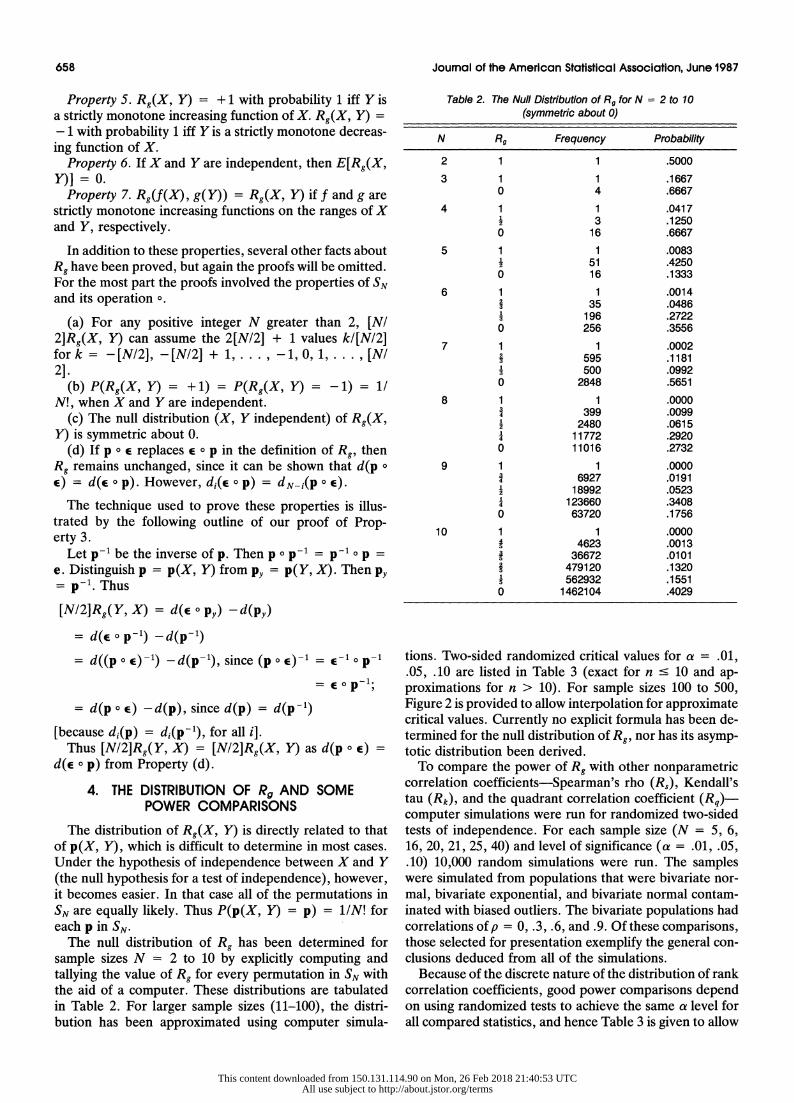
The null distribution of Rg has been determined for sample sizes N = 2 to 10 by explicitly computing and tallying the value of Rg for every permutation in SN with the aid of a computer. These distributions are tabulated

in Table 2. For larger sample sizes (11-100), the distri-

bution has been approximated using computer simula-

Table 2. The Null Distribution of Rg for N = 2 to 10

(symmetric about 0)

N Rg Frequency Probability

2 1 1 .5000

3 1 1 .1667 0 4 .6667

4 1 1 .0417

2 3 .1250 0 16 .6667

5 1 1 .0083

2 51 .4250 0 16 .1333

6 1 1 .0014

i 35 .0486 3 196 .2722 0 256 .3556

7 1 1 .0002 595 .1181 500 .0992

0 2848 .5651

8 1 1 .0000 4 399 .0099 2 2480 .0615 4 11772 .2920 0 11016 .2732

9 1 1 .0000

4 6927 .0191 2 18992 .0523 4 123660 .3408 0 63720 .1756

10 1 1 .0000 45 4623 .0013

36672 .0101

i 479120 .1320 5 562932 .1551 0 1462104 .4029

tions. Two-sided randomized critical values for a - .01, .05, .10 are listed in Table 3 (exact for n < 10 and ap- proximations for n > 10). For sample sizes 100 to 500, Figure 2 is provided to allow interpolation for approximate

critical values. Currently no explicit formula has been determined for the null distribution of Rg, nor has its asymptotic distribution been derived.

To compare the power of Rg with other nonparametric

correlation coefficients-Spearman's rho (Rs), Kendall's tau (Rk), and the quadrant correlation coefficient (Rq) computer simulations were run for randomized two-sided tests of independence. For each sample size (N = 5, 6, 16, 20, 21, 25, 40) and level of significance (a = .01, .05, .10) 10,000 random simulations were run. The samples were simulated from populations that were bivariate normal, bivariate exponential, and bivariate normal contaminated with biased outliers. The bivariate populations had

correlations of p = 0, .3, .6, and .9. Of these comparisons, those selected for presentation exemplify the general con- clusions deduced from all of the simulations.

Because of the discrete nature of the distribution of rank correlation coefficients, good power comparisons depend

on using randomized tests to achieve the same ae level for all compared statistics, and hence Table 3 is given to allow



.24

.22

.20

.18

.16

co

.14

o .12 t \ \ a. a .10 \ \ \ .01 C. .10

.08 N-. .05

~ _ .10 .06

-..20

.04

.02

I I I . 0 100 200 300 400 500

Sample Size, N

Figure 2. Interpolated Critical Values for a Randomized Two-Tailed Test of Independence, Using Rg(X, Y), for Samples of Sizes 100, 200, 300, 400, and 500 (based on simulations of size 2,500). Interpolated critical values = cl + p*(c, - c2), where cl > C2 and P(Rg 2 cd) + p*P(Rg = C2) = a.

possible future comparisons. To use Table 3 for a two- sided test with a c .10 for N = 33, reject the independence

hypothesis if IRg I 2 15; that is, use the column labeled Critl. To get a = .10 exactly, reject if IRgl 2 15 and reject with probability p = .4909 if |Rg| = 16

The biased outliers referred to previously are based on the type of bias that may occur when comparing judges' rankings, for example, in diving or gymnastics competi-

tion. For instance, two judges from rival regions may each

rank competitors from their own region more favorably than other competitors and rank those from the rival re-

gion more harshly. In the YMCA data, the YMCA di- rector's son was on the fourth best team! In the simulations

that were run, this bias was created by sampling from a bivariate normal distribution having the given correlation p and having standard normal marginal distributions. Then, if the first value of the pair sampled was an extreme

value (e.g., absolute value of the sample exceeds Za/2), the second value was negated. For example, if a = .05

and the pair sampled was (2, 1.5), then since 2> z.025 = 1.96, (2, 1.5) was replaced by the pair (2, -1.5) in the

sample to test the hypothesis of independence. This is an exaggerated biased outlier concept and hence is useful for detecting effects of such outliers.

As expected, simulations from a bivariate normal population showed that the power of Rg was better than that of the quadrant correlation coefficient (Rq) and not as good as that of Spearman's rho (Rs) and Kendall's tau (Rk). Figure 3 illustrates this for p = .6. The power of

the Pearson product moment correlation coefficient (Rp) was graphed for the same set of simulations.

When the sample was derived from a bivariate exponential population (Marshall and Olkin 1967), the power of Rg was better than that of the quadrant correlation (Rq) and not as good as Kendall's tau (Rk). Note, however, that the power of Rg was close to that of Rs. Moreover, the power of Rg overtook the power of the Spearman rho

(Rs) as the sample size increased. For larger samples the



Table 3. Critical Values for a Randomized Two-Tailed Test of Independence Using Rg(X, y),a for Samples of Sizes 2 to 100b

10% 5% 1%

N Criti Crit2 p Criti Crit2 p Critl Crit2 p

2 * .10000 * .05000 * .01000 3 * .30000 .15000 * .03000 4 4 4 .06667 .60000 4 .12000 5 4 4 .09804 4 .03922 4 .60000 6 4 4 .00000 4 .48571 4 .07429 7 4 4 .42185 4 .21008 4 4 .04067 8 4 4 .65161 4 .24516 4 .50276 9 4 4 .59056 4 4 .11289 4 4 .26179 10 4 4 .29250 4 4 .10316 4 4 .36867 11 4 4 .23640 4 4 .04260 4 4 .19350 12 4 4 .13820 4 4 .59640 4 4 .08190 13 .04960 4 .59530 .01480 14 4 .10300 4 .64540 . 55230 15 .94240 4 .36640 .50000 16 .65860 4 .40770 .48750 17 4 4 .76300 4 4 .40380 4 4 .20000 18 4 4 .76600 4 4 .34650 4 4 .17750 19 .50390 .34400 4 .06110 20 .41240 A .05320 .01510 21 1 .40810 .81180 A A .02740 22 .29500 A A .43330 1 .58820 23 1 A .27790 A .43150 A A .47060 24 1 .18570 .38160 1 .34440 25 A A .06400 A A .36730 A A5- .27400 26 A A .07220 A A .33850 A A .05260 27 1 .10510 1 .32930 1 1 .16410 28 4 - .95360 A 1 .22900 A 4 .06340 29 A A .81450 4 .18800 A 4 .92000 30 1 A .83330 1 1 .09480 A .75000 31 A .79740 A .00000 A A .63460 32 1 1 .63730 1 1 .01660 A A .67920 33 A A .49090 1 .92900 A 1 .53130 34 7 .50380 A P .62740 A 1 .47830 35 A .40050 .* 67940 A 17 .29730 36 1 .35230 A A .61810 1 1 .20730 37 A .33620 1 .54400 1 A .10620 38 1 .26040 A 1 .36090 1 A9 .02080 39 1 .26320 A .35360 1 .02220 40 .23800 A .29910 .05940 41 A A .14670 A A .31780 A A .87100 42 A .00810 A A .31090 A A .76320 43 .94700 A .16480 .40910 44 A .84330 A .14290 .37290 45 2 .86220 A .94510 22 .34380 46 .78920 A .08310 - .30190 47 .74230 A .88270 A 3 .10840 48 .61240 A .98560 A 4 .09590 49 .71890 A A .79680 2A .09520 50 A .55620 A A .65660 85- .17390 51 .43660 i * .58060 A A .75760 52 A .58200 A A .55630 A A .91180

powers of Rg and Rs were essentially equal, with that of Rg generally being slightly greater. Figure 4 illustrates this for p = .6. Again the power of the Pearson product

moment correlation coefficient (Rp) was included for comparison even though it is not appropriate for this

distribution.

When the samples were bivariate normal with the biased outlier contamination, the powers of the correlation coefficients were ordered as they were for the pure bivariate normal case when the sample was quite small. However, the power of Rg increased relative to the others as the sample size increased. Rg had the most power for larger

samples. Figure 5 illustrates this for simulations from a bivariate normal with p = .6, which was contaminated by biased outliers as explained earlier.

Further study of biased outliers showed that Spearman's rho (Rs) and Kendall's tau (Rk) often rejected the null hypothesis of independence in the wrong direction, whereas Rg rarely did. That is, when p > 0, the rejection was frequently due to the sample correlation being more negative than the negative critical value. In this case we shall say that the null hypothesis was incorrectly rejected.

The Pearson product moment correlation coefficient (Rp) is extremely sensitive to this contamination. Table 4 gives



Table 3 (continued)

10% 5% 1%

N Criti Crit2 p Criti Crit2 p Criti Crit2 p

53 A A .51160 A A .57320 A A .55260 54 .26920 7 1 .42960 P A .57690 55 A .32860 7 A .49870 P 7 .75860 56 A .24570 Af A .13710 A .55000 57 A A .30410 Af A .31330 BA .33330 58 A A .12240 YA .31290 .16670 59 A .06640 A .13770 .18000 60 .07990 .13490 .05560 61 .11670 .00550 .05450 62 .01990 .95240 .04240 63 .04650 T .05740 .06370 64 .89510 .91180 .87440 65 .86900 .78620 .71920 66 3A .84880 A .81300 A .79170 67 A A .63290 A .77600 A .58620 68 h A .71190 A .75000 A .75000 69 4 A .66500 A .61310 A .57690 70 A A .82900 A .39040 A .30560 71 5 A .53970 A 5 .47370 A .36110 72 A .58200 A - .33820 A .25000 73 A .41960 A .25640 A .10260 74 7 A .51880 A .39390 .13640 75 i A .37900 A .30720 ? .25580 76 1 A .32220 A .14570 A .08700 77 1 A .31350 A .35250 A .31580 78 A A .31490 A A .14570 A .04000 79 A A .22090 A A .01430 a .64710 80 a A .22050 A a .03390 a .60000 81 4i A .21190 A a .05260 a .16670 82 A A .14910 A .75440 i 4? .92310 83 A4 A .09230 A .92310 .16670 84 4A .08940 A .86000 4 .50000 85 A .02960 A .78460 4A .06900 86 -A .86460 h .88890 a .38460 87 A -A .95450 h A .64290 A .03330 88 f4 A .04170 A A .79590 V .00000 89 4i A .05000 A A .77080 R .91670 90 A fi .69880 A A .61710 4 5 .85710 91 A A .55170 A A .43860 i .33330 92 A li .55790 A A .37500 4 .00000 93 A .64710 .32260 4 .28570 94 7 .63640 4 .48280 4 .12500 95 4 .63830 1 .39240 H * .27270 96 A A .51550 A A .16070 14 .20000 97 A A .55240 T A .28570 4 .25000 98 A .59520 A .13640 i 4 .52940 99 A .61860 A A .07790 f .68750 100 A A .35710 A A .00000 1 A .72730

a Example: To obtain a two-sided test with a = .05 for N = 15, reject Ho independent variables if IRgl 2 - and reject Ho with probability p = .36640 if IRgl = . b The values are based on the exact distribution of Rg(X, Y) for N = 2 to 10 and on simulations (of size 10,000) for N = 11 to 100; thus the fifth decimal place (0) for N > 11 appears only

as a visual convenience.

the results from 1,000 simulations of samples of the stated size from a bivariate normal population with the indicated correlation (p) and with biased outlier contamination. Consequently, for one-sided alternatives the power of Rg would be better relative to that of the other sample correlations.

5. TIED RANKS

A summary of tied rank procedures appears in H'ajek and gidak (1967, pp. 118-123), and we will assume that the reader is familiar with the randomization technique. For many data sets with tied values, Rg assumes only one

value, and hence we recommend the randomization method so that Tables 2 and 3 can be used. We also recommend that the highest and lowest values of Rg be com- puted over the range of possible randomizations. If it is found that the difference between these values is large, then the conclusion should be drawn that there is little information in the data set.

To determine the extreme values of Rg, the two randomizations of p that most favor positive and negative correlation are determined.

Let us demonstrate the suggested procedure by taking an example from Conover (1980, example 1, p. 253). This



1.0 8R

_-.--- _ *-, Rk

0~ ~ ~ ~~~~~~~~ 6 / Rq

Rg

0.8

I.~ ~ ~ ~ ~~~*

~~~/ Rp Paro

q

0.6 1

a.~~~~~~~~~~ .

0 /100304

0.4

0.2 1 / ,_ _

t ~~~~~~~~Rg: Greatest / // ~~~~~~~Rk: Kendall

R -p :Pearson ---Rq: Quadrant

RS: Spearman

0 1 0 20 30 40

Sample Size, N

Figure 3. Relative Powers of Randomized Tests of Independence From a Bivariate Normal Population Based on 10,000 Simulations for Each of N = 5, 6, 16, 20, 21, 25, and 40 (p = .6, a = .05, two-tailed tests).

example is chosen because the tied rank procedure is dis- cussed there for Rs and Rk. The data are from psycholog- ical tests on identical twins, with X being the first born.

The data given are in the well-known mid-rank form:

X 1 2 3.5 3.5 5 6.5 6.5 8 9 10 11.5 11.5

Y 1 2.5 8 7 4.5 6 2.5 10 4.5 9 12 11

From Conover, Rs = .7378 or .7354 depending on which formula is used for Rs, and Rk = .5606. The approximate probability values for the two-sided test are given as .01

for both Rs and Rk. To obtain the randomization of this tied data that most

favors positive correlation, one simply chooses the lowest possible rank for Y as one proceeds over the 12 ranks of X within the constraints of the tied values. The permutation obtained is the same if the roles of X and Y have

been interchanged. In a similar manner the permutation

most favoring negative correlation is determined. We list these two permutations:

X 1 2 3 4 5 6 7 8 9 10 11 12

Y(+ correlation) 1 2 7 8 4 3 6 10 5 9 11 12

Y(- correlation) 1 3 8 7 5 6 2 10 4 9 12 11

In both cases Rg = (4 - 2)/6 = 1 and hence all random-

izations would give Rg = 2. For N = 12, Rg is significant at the 10% level, significant with probability .5964 at the

5% level, and significant with probability .0819 at the 1% level.

Thus, for this data set, the use of Rg leads to 10% significance, whereas Rs and Rk are approximate tests significant at the 1% level but based on limiting distributions



1.0 Rs

0.8

0.61

0 0-

0.4--~~~4

0.2 1

f/- - Rg: Greatest .. Rk: Kendall

Rp: Pearson - - - Rq: Quadrant

RS: Spearman

0 10 20 30 40

Sample Size, N

Figure 4. Relative Powers of Randomized Tests of Independence From a Bivariate Exponential Population Based on 10,000 Simulations for Each of N = 5, 6, 16, 20, 21, 25, and 40 (p = .6, a = .05, two-tailed tests).

that may be unreliable for small sample sizes. A possible use of Rg as an exact test for data sets with tied values would certainly help an experimenter in evaluating his data, especially when the sample size is very modest, as in this example.

The above data set was one of several that were checked in various nonparametric statistics books. Most led to one value of Rg. Suppose, however, that the X variable had all distinct ranks but all N Y ranks were tied. Then the rejection of the null hypothesis would be unrelated to the gathered data but would be entirely due to the randomization procedure. In this case the two extremes of Rg would be in -1 and +1 and all experimenters would realize that there is no information in their data relating X and Y. Note also that in this case, the average of the two extreme possible values of Rg would be 0.

The use of mid-ranks is well established for many rank

statistics, but after some study, no satisfactory way was found for their use with Rg. On the other hand, the idea of determining the highest and lowest statistic over the range of possible permutations within the constraints of tied data might be beneficial descriptive statistics for other statistics besides Rg.

6. POPULATION INTERPRETATION OF Rg

Kruskal (1958) gave a population interpretation to Rs, Rk, and Rq. It is possible also to relate the correlation statistic Rg to a population parameter. Assume that a bivariate random variable (X, Y) is absolutely continuous and that a sample of size N is to be drawn. Let X(i), Y(1) be the order statistics. It is straightforward to show that for Rg(X, Y) the quantity di(p)li equals, within the sample, the proportion of cases in which Y > Y(1) given X c



0.5

Rg

Rk

0.4 .

0. 0.2* //p

. //

0.1 / Rg: Greatest /w*- * - Rk: Kendall

Rp: Pearson

- - - Rq: Quadrant

R:S Spearman

0 10 20 30 40

Sample Size, N

Figure 5. Relative Powers of Randomized Tests of Independence From a Bivariate Normal Population With 10% Biased Outliers Based on 10,000 Simulations for Each of N = 5, 6, 16, 20, 21, 25, and 40 (p = .6, a = .05, one-tailed tests).

X(i). Likewise, di(E o p)Ii equals the proportion of cases in which Y < Y(N+1-i) given X < X(i). Thus di(p)Ii is an estimate of P(Y > Y(i) j X c X(i)) and di(E o p)Ii is an estimate of P(Y < Y(N+l-i) X c X(i)). For i = 1,

2, ... , N, P(Y > Y(O) I X s X(i)) is the standardized area of a series of rectangles [corner at (X(i), Y(i))], which are open toward the upper left if we let X be the abscissa and Y be the ordinate axes. Similarly, as i = 1, 2, . .. , N

P(Y < Y(N+l-i) I X - X(i)) is the standardized area of a series of rectangles [corner at (X(i), Y(N+1-i))], which are open toward the lower left.

To simplify matters let us use the probability integral transformation as was done in Kruskal (1958). Let U = F(X) and V = G(Y), where F and G are the marginal cdf's of X and Y, respectively. Then for the joint density of (U, V), the marginals will be U(O, 1). Let U(i), V(i) be the order statistics for random variables U, V; (U, V) are

called the grades in Kruskal. Then di(p)I[NI2] will estimate

(il[N12])P(U s< U(i), V > V(i,)IP( U < uoi),

and di(e o p)I[N12] will estimate

(il[N12])P(U C U(i), V < V(N+1-i))IP(U c U(i)).

For N large, U(i) approaches its expectation il(N + 1), and since P(U c il(N + 1)) = il(N + 1) and ([N12]Ii) * (il(N + 1) approaches 2, for large N and letting il(N + 1) -t

Rg = max di(E o p)I[N12] - max di(p)I[NI2]

estimates

sup 2P(U t, V < 1 - t) - sup 2P(U < t, V > t). O<t<l O<t<l



Table 4. Wrong Direction Rejection Comparisons for Biased Outlier Simulations

Correlation Total number Number incorrectly coefficient rejected rejected

Sample size = 20, p = .2, 1,000 samples

Rg 34 7 Rk 56 32 Rs 55 30 Rp 57 40

Sample size = 21, p .8, 1,000 samples

Rg 138 2 Rk 140 49 R, 113 57 Rp 263 229

Before proceeding with examples, let us relate the pre- vious formula to the copula function C used in Schweizer and Wolfe (1981).

P(U < t, v < 1 - t) = C(t, 1 -t)

and

P( U -S t, V > t) =C(tq 1) C(tg t) -

Thus in the limit

Rg = 2 sup C(t, 1 - t)-2 sup [C(t, 1) - C(t, t)]. O<t l O<t<l

Now as stated in Schweizer and Wolfe (1981),

C(u, v)

= max(u + v - 1, 0) for perfect negative correlation

= uv if independent

= min(u, v) for perfect positive correlation.

Thus C(t, 1 - t) = 0 for perfect positive correlation and hence sup C(t, 1 - t) - 0 measures the distance from perfect positive correlation. Likewise, C(t, 1) - C(t, t) = 0 for perfect negative correlation and sup[C(t, 1) - C(t, t)] - 0 measures the distance from perfect negative

correlation. The quantity K(X, Y) = 4 supo<u,v<l C(u, v) - uvj was introduced by Blum, Kiefer, and Rosenblatt (1961) as a test of independence, but it was not developed for practical use and its asymptotic distribution was not derived. In contrast to Rg their statistic measures distance from independence, and the sample statistic form

K = 4 sup[Hn(X, y) -En(x)Gn(Y)] x,y

where Hn, Fn, Gn are empirical distribution functions, needs a computer for evaluation even for small sample sizes.

We now give two examples to show that Rg can sometimes behave like Kendall's tau and sometimes like Spear- man's rho. If (X, Y) is bivariate normal, say

then for large N, Rg estimates the same quantities as Ken-

dall's z, (2Iir)sin-tp. To see this, we make the probability

integral transformation and then C(u, v), the copula function, is the bivariate cdf of (U, V). Then for large N,

Rg = sup 2C(t, 1 - t) - sup 2(t - C(t, t)) O<t<l O<t<l -

(2 2) (2 (2 2)

=(24 + 17 sin p)I - 2 (1 - 2-sin -lp)

2 - - sin- p,

because the bivariate normal has maximum probability of open rectangles at the medians. If p = , then Rg = Rk

= (2/I)sin- X .5399 and R, = (6/7r)sin-1(p/2) = .7341. It is not true that Rg always estimates the same quantity

that Rk does. To show this, take the following example, where the density of U, V is

g(u, v) = 2 for 0 s u, v c 2 and for 1 c u, v c 1

= 0 elsewhere.

Then the marginals are U(O, 1) and it is straightforward

to show that p = Rs = Rg = 43, but Rk 1 Finally, if X and Y are independent, then so are U and

V. In this case maxi di(p)I[NI2] and max, di(e o p)I[N12] both estimate A and Rg estimates supo<t<l 2t(1 - t) - supo<t<i 2(t - t2) = 0.

7. FINAL COMMENTS

It should be noted that in the biased outlier simulations the quadrant correlation coefficient (Rq) also increased in

power relative to R. and Rk, becoming second to Rg for large samples. Rq is closely related to a correlation coefficient defined similarly to Rg but based on the deviation at only one point instead of the maximum deviations at all points. All results are stated without proofs, which are tedious but straightforward (Hollister 1984). To see this,

define, for an integer 0 < i < N, Ri(X, Y) as follows: Ri(X, Y) = (di(e o p) - di(p))INi, where p = p(X, Y) and Ni = min(i, N - i). Under the null hypothesis of independence between X and Y, di(p) and di(E o p) are hypergeometric random variables and Ri(X, Y) has the probability function

f(x) = P(Ri(X, Y) = x)

, Nij Ni N-2N j /Nh + jNixJ \2j +(x- 1)N/ VNi}

forx= -1, -1 + 1INi, -1 + 2INi, . . . , + 1. ForN

even, R[N,21 = R1(N+1),21 = Rq; for N odd, however, R[NI2], R[(N+ 1)/21, and Rq may differ slightly but R[N/2] and R[(N+1)/2] have the same distribution, which is asymptoti- cally equivalent to the distribution of Rq.

In conclusion, we have defined a maximum deviation type nonparametric correlation coefficient Rg for use in

testing the hypothesis of independence between two random variables. Moreover, Rg could be considered as a



generalization of the quadrant correlation coefficient, Rq. Furthermore the power of Rg falls among that of other well-known nonparametric correlation coefficients when the sample comes from a bivariate normal, is as good as

Rs for larger sample sizes of a bivariate exponential population, and is greater than that of the others when the population is a bivariate normal contaminated with biased outliers and the sample sizes are large. In addition, if a sample is severely biased in one of the tails (or, equiva- lently, the correlation is reversed from the bulk of the data in one of the tails), then Rg senses the correlation in the bulk of the data best. Thus Rg may be especially useful in problems in which outliers are present, contaminated populations are involved, or certain types of nonlinearity occur in bivariate data.

There are possible uses for Rg beyond just independence testing. For example, some forms of cluster analysis depend on the correlation coefficient as a measure of dis-

tance. This new coefficient used on nonnormal data could possibly cluster the data in a more attractive manner.

[Received May 1985. Revised August 1986.]

REFERENCES

Blomqvist, N. (1950), "On a Measure of Dependence Between Two Random Variables," Annals of Mathematical Statistics, 21, 593-600.

Blum, J. R., Kiefer, J., and Rosenblatt, M. (1961), "Distribution-Free Tests of Independence Based on the Sample Distribution Function," Annals of Mathematical Statistics, 32, 485-498.

Conover, W. J. (1980), Practical Nonparametric Statistics, New York: John Wiley.

Hajek, J., and Widak, Z. (1967), Theory of Rank Tests, New York: Academic Press.

Hollister, R. A. (1984), "A Correlation Coefficient Based on Maximum Deviation," unpublished Ph.D. dissertation, University of Montana, Dept. of Mathematical Sciences.

Kendall, M. G. (1938), "A New Measure of Rank Correlation," Bio- metrika, 30, 81-93.

Kruskal, W. (1958), "Ordinal Measures of Association," Journal of the American Statistical Association, 53, 814-861.

Marshall, A. W., and Olkin, I. (1967), "A Multivariate Exponential Distribution," Journal of the American Statistical Association, 62, 30- 44.

Renyi, A. (1959), "On Measures of Dependence," Acta Mathematica Academiae Scientiarum Hungaricae, 10, 441-451.

Schweizer, B., and Wolfe, E. F. (1981), "On Nonparametric Measures of Dependence for Random Variables," The Annals of Statistics, 9, 879-885.

Spearman, C. E. (1904), "The Proof and Measurement of Association Between Two Things," American Journal of Psychiatry, 15, 72-101.


a rank correlation coefficient resistant to outliers

Documents