1

Application of Nonlinear Autoregressive with Exogenous Input

(NARX) neural network in macroeconomic forecasting, national goal

setting and global competitiveness assessment

Liyang Tang1, *

1Research Bureau, People’s Bank of China, Beijing 100800, China; tliyang@pbc.gov.cn

*Correspondence: tliyang@pbc.gov.cn; Tel.: +86-10-13581917180

2

Abstract:

As the trove of economic big data released by statistical agencies, private and public surveys, and

other sources every day becomes continuously available in real time, making high-quality

economic forecasts requires tracking a large and complex set of data, however, the limited

deductive and inductive abilities of the human brain or the inadequacies of current econometric

approaches and other modeling methods greatly limit the above full use of the trove of economic

big data. But with the rapid development of neural network methods and their cross-field

applications in recent years, certain types of neural networks such as the Nonlinear Autoregressive

with Exogenous Input (NARX) neural network may be considered as a general method of making

full use of the trove of economic data to make time series predictions. This paper selects the

NARX neural network as the method of this study through literature review, and constructs

specific NARX neural networks under specific application scenarios involving macroeconomic

forecasting, national goal setting and global competitiveness assessment, where after this study

focuses on analyzing how different settings for exogenous inputs from the trove of economic big

data affect the prediction performance of NARX neural networks. Next, through case studies on

China, US and Eurozone, this study wants to explore and summarize how those limited & partial

exogenous inputs or abundant & comprehensive exogenous inputs, a small set of most relevant

exogenous inputs or a large set of exogenous inputs covering all major aspects of the macro

economy, whole area related exogenous inputs or both whole area and subdivision area related

exogenous inputs specifically affect the forecasting performance of NARX neural networks for

specific macroeconomic indicators or indices. And next, through the case study on Russia this

paper similarly explores how the limited & most relevant exogenous inputs set or the abundant &

comprehensive exogenous inputs set specifically influences the fitting performance and prediction

performance of those specific NARX neural networks for national goal setting. Finally,

comparative studies on the application of NARX neural networks for the forecasts of Global

Competitiveness Indices (GCIs) of various economies are conducted, in order to explore whether

the specific NARX neural network trained on the basis of the GCI related data of some economies

can make sufficiently accurate predictions about GCIs of other economies, and whether the

specific NARX neural network trained on the basis of the data of some type of economies can

3

give more accurate predictions about GCIs of the same type of economies than those of different

type of economies. Based on all of the above successful application, this paper provides policy

recommendations on applying fully trained NARX neural networks that are assessed as qualified

to assist or even replace the deductive and inductive abilities of the human brain in a variety of

appropriate tasks.

Keywords: Nonlinear Autoregressive with Exogenous Input (NARX) neural network;

macroeconomic forecasting; goal setting; competitiveness assessment; leading business and

economic indicators and indices

4

1. Introduction

The trove of economic big data released by statistical agencies, private and public surveys,

and other sources is parsed every day by not only governments and authorities, but also

economists and market analysts. The governments and authorities usually parse the trove of

economic big data in order to assist decision-making, and making forecasts on the basis of the

trove of economic big data is also essential to governments and authorities in informing their

policy decisions and communicating their economic outlook to the public. Economists usually

parse the trove of economic big data to assess the health of the economy and serve specific

research topics. Market analysts usually strive to parse the most valuable part of the trove of

economic big data, in order to understand where the economy currently is and to forecast in which

direction it is going, which can provide direct and indirect market value.

However, the full use of the trove of economic big data is not that easy. For example,

although monitoring a large number of different economic indicators and indices to detect early

signals, which not only enables one to exploit different sampling frequencies and different timing

of macroeconomic data releases, but also mitigates the risk of overweighting idiosyncratic

fluctuations as well as measurement errors, can enhance timeliness and accuracy in assessing the

health of the economy, separating meaningful signals from noise for each indicator or index and

integrating the extracted information (sometimes even contradictory) into a single conclusion are

always difficult tasks with no fixed solution (Bok et al., 2017). Take another example, as the trove

of economic big data becomes continuously available in real time, making high-quality economic

forecasts to help understand where the economy is now requires tracking a large and complex set

of data, since information about different aspects and sectors of the economy can be considered as

imperfect measures of latent economic situations, the more systematic and comprehensive the

information, the higher the quality of prediction, however, the limited deductive and inductive

abilities of the human brain or the inadequacies of current econometric methods and modelling

methods (such as can’t provide economic forecasts at high frequency) greatly limit the above full

use of the trove of economic big data, then forecasters could either only track a small number of

key and comprehensive indicators of economic activity to make predictions, or use complicated

mathematical models to form projections and apply subjective adjustments to pure

5

model-generated forecasts, or use a combination of a suite of models and a fair amount of expert

judgment to generate forecasts, all of the above workarounds are just stopgaps and

problem-specific solutions, and cannot be regarded as general methods of making full use of the

trove of economic big data to make predictions (Ghoddusi et al., 2019; Ozbayoglu et al., 2020).

With the development of a large number of machine learning methods and their cross-field

applications, representative machine learning methods such as neural network methods have been

well equipped to exploit the trove of economic big data more effectively and efficiently than

traditional econometric or modeling methods, in other words, certain types of neural networks

may be considered as a general method of making full use of the trove of economic big data to

make predictions (Bok et al., 2017; Storm et al., 2019). Compared with current econometric

approaches and other modeling methods, neural network methods that focus on making

predictions have the following advantages: first, neural networks are highly flexible and may be

helpful in settings where other flexible models have computational problems due to the size of the

dataset or the number of economic variables that need to be considered; second, neural network

approaches can automatically extract the most relevant features for a prediction task, and are

potentially capable of deriving more complex features from the raw data that are missed by other

approaches; third, neural network methods can be useful in addressing problems with large

number of explanatory variables, and they are especially crucial and almost irreplaceable when the

number of explanatory variables exceeds the number of observations in large datasets; fourth, the

predictive ability of neural networks in complex and high-dimensional settings can be used to

improve causal estimates under some application scenarios (Storm et al., 2019).

Since neural network methods that are specifically developed for making predictions have

already demonstrated great potential in improving prediction, then the idea of this study is to

first determine both the specific type of neural network and the specific application

scenarios that have important economic significance but have not been systematically and

deeply studied, and then apply this particular type of neural network to these specific

economic scenarios, in order to focus on analyzing how different settings for exogenous

inputs from the trove of economic big data affect the prediction performance of neural

networks.

6

The remainder of this paper is structured as follows. The literature review in the next section

focuses on the systematic and comprehensive search for application of neural networks in various

subfields of economics and finance from the most representative academic and policy studies,

which are used to provide inspiration to either the determination of specific application scenarios

or the selection of specific neural network methods in our study. Section 3 selects and introduces

the Nonlinear Autoregressive with Exogenous Input (NARX) neural network, and constructs

specific NARX neural networks under various specific application scenarios including

macroeconomic forecasting, national goal setting and global competitiveness assessment, so that

the subsequent studies can focus on analyzing how different settings for exogenous inputs affect

the prediction performance of NARX neural networks. Section 4 carries out the application of

NARX neural networks for macroeconomic forecasting in the form of case studies on China, US

and Eurozone, in order to explore and summarize how those limited & partial exogenous inputs or

abundant & comprehensive exogenous inputs, a small set of most relevant exogenous inputs or a

large set of exogenous inputs covering all major aspects of the macro economy, whole area related

exogenous inputs or both whole area and subdivision area related exogenous inputs specifically

affect the forecasting performance of NARX neural networks for specific macroeconomic

indicators or indices. Section 5 similarly explores how the limited & most relevant exogenous

inputs set or the abundant & comprehensive exogenous inputs set specifically influences the

fitting performance and prediction performance of those specific NARX neural networks for

national goal setting, through the case study on Russia. Section 6 conducts comparative studies on

the application of NARX neural networks for the forecasts of Global Competitiveness Indices

(GCIs) of various economies, in order to simply and intuitively explore whether the specific

NARX neural network trained on the basis of the GCI related data of some economies can make

sufficiently accurate predictions about GCIs of other economies, and whether the specific NARX

neural network trained on the basis of the data of some type of economies can give more accurate

predictions about GCIs of the same type of economies than those of different type of economies.

Section 7 offers policy recommendations on applying fully trained NARX neural networks that

are assessed as qualified to assist or even replace the deductive and inductive abilities of the

human brain in a variety of appropriate tasks. Section 8 concludes.

7

2. Literature Review

In this section we systematically and comprehensively search for application of neural

networks in both empirical and normative fields of economics and finance from the most

representative academic and policy studies, which could be used to provide enlightenment for this

study not only in the selection of specific neural network methods, but also in the determination of

specific application scenarios such as economic & financial forecasting, government

decision-making and policy evaluation that have not been systematically and deeply studied.

If we have to pick not only the hottest but also the most representative application areas for

neural network methods among various economic and financial subfields, that must be the various

subfields of energy economics and finance. More specifically, the application of neural networks

covers areas such as energy prices prediction, energy demand or consumption forecasting,

structure of energy system, energy policy analysis, model calibration, energy trading strategies,

and data management. Neural network methods can provide superior performance for forecasting

energy prices because they have higher flexibility in handling energy commodity price series that

typically demonstrate complex features such as non-linearity, lag-dependence, non-stationarity,

and volatility clustering (Cheng et al., 2018; Ghoddusi et al., 2019). Among literatures about

energy price predictions, a vast majority of papers focus on either crude oil price prediction

(Cheng et al., 2018; Ding, 2018; Godarzi et al., 2014; Huang and Wang, 2018; Jammazi and Aloui,

2012; Moshiri and Foroutan, 2006; Safari and Davallou, 2018; Wang and Wang, 2016; Yu et al.,

2008; Yu et al., 2017; Zhao et al., 2017) or electricity price prediction (Aggarwal et al., 2009;

Bento et al., 2018; Conejo et al., 2005; Dudek, 2016; Lago et al., 2018; Panapakidis and

Dagoumas, 2016; Peng et al., 2018; Singh et al., 2017; Wang et al., 2017; Weron, 2014; Yang et al.,

2017); papers on predicting natural gas prices (Čeperić et al., 2017; Nguyen and Nabney, 2010)

and carbon prices (Fan et al., 2015; Sun et al., 2016) are much less frequent, while major papers

on predicting coal prices are hard to be found, even though coal is a major energy source. Since

government agencies and financial & trading institutions are all interested in having a realistic

forecast of energy consumption portfolio in the future, a vast majority of literatures make

long-range predictions of aggregate and sectoral energy demand based on neural network methods

(Debnath and Mourshed, 2018; Geem and Roper, 2009; Kaytez et al., 2015; Liu et al., 2016;

8

Sözen and Arcaklioglu, 2007; Sözen et al., 2007; Xiao et al., 2018), among different types of

energy, electricity demand forecasting is the most traditional domains for neural network methods

(Ardakani and Ardehali, 2014; Azadeh et al., 2008; Lai et al., 2008; Pao, 2006), and neural

network is much better suited for short-term electricity demand forecast than the national level

forecast, since the electricity sector can provide a large number of high-frequency observations on

a large set of potential input variables (Anderson et al., 2011; Bassamzadeh and Ghanem, 2017;

Liu et al., 2014), however, there are less neural network related literatures on predicting natural

gas demand (Azadeh et al., 2010; Panapakidis and Dagoumas, 2017; Szoplik, 2015), on predicting

transport energy demand (Geem, 2011; Limanond et al., 2011; Murat and Ceylan, 2006), and on

predicting coal demand (Hu et al., 2008; Ning, 2003; Yang et al., 2014). Among other relatively

minor application areas of the neural network approach, there are relatively abundant studies on

structure of energy system (Ermis et al., 2007; Fang et al., 2013; Farajzadeh and Nematollahi,

2018; Skiba et al., 2017; Sözen, 2009; Zhang et al., 2016), and researches on energy policy

analysis are also relatively easy to be found (Dagoumas et al., 2017; Mahmoud and Alajmi, 2010;

Skiba et al., 2017), while studies on model calibration (Sun et al., 2011), on energy trading

strategies (Moreno, 2009), and on data management (Abdella and Marwala, 2005; Nelwamondo et

al., 2007) are the least frequent.

If the merits and limitations of neural network methods are compared horizontally among all

machine learning methods that have already been applied to some subfield of energy economics

and finance, then accuracy in general, speed of classification, dealing with binary/continuous

attributes, and attempts for incremental learning are all considered to be the outstanding merits of

most neural network methods, while relatively low speed of learning, relatively low tolerance to

missing values, relatively low tolerance to irrelevant attributes, relatively low tolerance to

redundant attributes, relatively low tolerance to data noise, dealing with danger of overfitting, lack

of explanation ability or statistical inference, black box nature that leads to difficulties in

understanding how the results were obtained compared to other more transparent methods, and no

general rules for model parameter handling are considered as the limitations of some neural

network methods in some situations but not always (Ghoddusi et al., 2019). Among all kinds of

neural networks, the NARX neural network usually has a higher level of accuracy, superior

9

generality and practicability for time series prediction because of various advantages such as the

ability to keep a memory of past events to predict future trends (Wang and Wang, 2016), the

capacity to provide better forecasting accuracy than traditional time series analysis, especially in

the multi-step ahead short-term forecast (Cheng et al., 2018), its special structure that allows the

algorithm to automatically and efficiently model a high degree of complexity not only in the

interaction among various exogenous inputs, but also in the possible relationships between inputs

and outputs (Hatcher and Yu, 2018; LeCun et al., 2015), the ability to provide a high degree of

flexibility to address features as including a large number of exogenous variables in time-series

models, in other words, the ability to accept almost any number of exogenous inputs, which

relieves the neural network builder from the task of picking a small number of informative input

variables (Zhao et al., 2017), the flexibility of outputs depending on the problem under study, in

other words, the flexible and changeable application of the same type of NARX neural network in

various problems such as regression problems, classification problems or ranking problems

(Ghoddusi et al., 2019), and no special data preprocessing required, for example the detrending,

seasonal adjustment, or decomposition of the time series, since the NARX neural network can

consider those characteristics as additional features of the data and incorporate them into the final

forecasting algorithm (Dudek, 2016).

Subfields of finance such as algorithmic trading, risk assessment, fraud detection, portfolio

management, asset pricing and derivatives market (such as options, futures, and forward contracts),

cryptocurrency and blockchain studies, financial sentiment analysis and behavioral finance, and

financial text mining are also among the hottest application areas for neural network methods

where specific neural networks are developed to provide real-time working solutions for the

financial industry (Ozbayoglu et al., 2020). For the sake of simplicity, we only state and compare

the major conclusions from those representative reviews of neural network-related studies in each

of the above subfields as follows. Algorithmic trading is defined as buy-sell decisions made solely

by algorithmic models, since financial time series forecasting is highly coupled with algorithmic

trading, most of the algorithmic trading studies have been concentrated on the prediction of stock

or index prices, meanwhile, the various types of recurrent neural networks (RNNs) have been the

most preferred neural networks in this subfield, since various types of trade indicators and

10

technical indicators that provide either real-time information or historical information can be

simply treated as the exogenous inputs into RNNs to help improve the quality of forecasts (Hu et

al., 2015; Ozbayoglu et al., 2020; Sezer et al., 2019). Risk assessment studies that adopt neural

networks as the method identify the riskiness of any given asset, firm, person, product, and bank,

and form various research topics such as bankruptcy prediction, credit scoring, credit evaluation,

loan/insurance underwriting, bond rating, loan application, consumer credit determination,

corporate credit rating, mortgage choice decision, financial distress prediction, and business

failure prediction, among various machine learning methods, a great number of researches have

turned their attention to specific neural networks such as the deep neural networks (DNNs) for

higher accuracy (Chen et al., 2015; Fethi & Pasiouras, 2010; Kirkos & Manolopoulos, 2004;

Kumar & Ravi, 2007; Lahsasna et al., 2010; Lin et al., 2012; Marqués et al., 2013; Ozbayoglu et

al., 2020; Ravi et al., 2008; Sun et al., 2014; Verikas et al., 2009). Financial fraud is one of the

areas where the governments and authorities are desperately trying to find a permanent solution,

that’s one important reason why fraud detection is also among the hottest application areas for

neural network methods, most of the studies in this area can be considered as anomaly detection

and are generally classification problems between fraud and non-fraud, and those neural networks

that specialize in accurate classification are usually adopted by these studies, for example the

convolutional neural networks (CNNs) (Kirkos et al., 2007; Ngai et al., 2011; Ozbayoglu et al.,

2020; Phua et al., 2010; Sharma & Panigrahi, 2013; Wang, 2010; West & Bhattacharya, 2016; Yue

et al., 2007). Portfolio management, which is the process of choosing various assets within the

portfolio for a predetermined period, covers those closely related and even interchangeable areas

such as portfolio optimization, portfolio selection, and portfolio allocation, since portfolio

management is actually an optimization problem, identifying the best possible course-of-action for

selecting the best-performing assets for a given period, as a result, a lot of neural networks that

specialize in solving optimization problems, such as RNNs and CNNs, have been developed for

this purpose (Li & Hoi, 2012; Metaxiotis & Liagkouras, 2012; Ozbayoglu et al., 2020). Asset

pricing and derivatives market (options, futures, forward contracts) are almost destined to be one

of the application areas for neural network methods, since accurate pricing or valuation of an asset

is a fundamental study area in finance, among a vast number of special neural networks developed

11

for banks, corporates, real estate, derivative products, etc., specially designed RNNs and DNNs

are usually proved to be more capable of assisting the asset pricing researchers or valuation

experts (Ozbayoglu et al., 2020). Since price forecasting and trading systems dominate the area of

cryptocurrency and blockchain studies, then application of neural network methods in this area is

similar to that in the area of algorithmic trading, which we’ve already mentioned above

(Ozbayoglu et al., 2020). Since emotion or investor sentiment is among the most important

components of behavioral finance, neural network methods are increasingly applied to financial

sentiment analysis, especially for trend forecasting, since most of the researches in this area are

focused on financial forecasting and based on text mining, then specially constructed RNNs,

DNNs, and CNNs are used most often in these researches (Kearney & Liu, 2014; Ozbayoglu et al.,

2020). With the rapid spreading of social media and real-time streaming news, instant text-based

information retrieval has become available, as a result, financial text mining studies have been

more and more popular in recent years, in fact text mining is usually accompanied by the semantic

analysis and forecast application of the extracted information, such as those financial sentiment

analysis coupled with text mining for forecasting, which we’ve already mentioned above, and text

mining without sentiment analysis for forecasting, which we haven’t talked about yet, and various

types of specially designed RNNs are the most widely and frequently used neural networks in both

types of studies (Kumar & Ravi, 2016; Li, 2011; Loughran & McDonald, 2016; Mitra & Mitra,

2012; Mittermayer & Knolmayer, 2006; Ozbayoglu et al., 2020).

Some newly developed representative and interesting application areas for neural network

methods and even machine learning methods in a broader sense in recent years that can offer

inspiration to either the determination of specific application scenarios or the selection of specific

neural network methods in our study are also briefly described as follows.

Recent literatures that can provide inspiration for application scenario determination are

presented as follows. Bandiera et al. (2020) use an unsupervised machine learning algorithm to

measure the behavior of CEOs in large samples via a survey that collects high-frequency,

high-dimensional diary data, this algorithm uncovers two distinct behavioral types that are leader

type and manager type, and its ability of accurate classification is proved to be much higher than

other traditional methods. Sabahi & Parast (2020) use predictive analytics by proposing a machine

12

learning approach to predict individuals’ project performance, which is considered as a new

measurement system for predicting performance. Mittal et al. (2019) monitor the impact of

economic crisis on crime in India through machine learning methods, which are proved to be

capable of automatically predicting the factors that affect the crimes effectively and efficiently.

Sansone (2019) helps high schools obtain more precise predictions of student dropout through

exploiting the available high-dimensional data from 9th grade jointly with machine learning tools,

which are proved to perform much better than the parsimonious early warning systems as

implemented in many high schools. Erel et al. (2018) demonstrate that machine learning

algorithms can even assist firms in their decisions on nominating corporate directors, specifically

speaking, machine learning holds promise for understanding the process by which governance

structures are chosen, and has potential to help real-world firms improve their governance.

Kleinberg et al. (2018) take bail decisions as a good test case, and prove that although machine

learning can be valuable when it is used to improve human decision making, realizing this value

requires integrating these tools into an economic framework: being clear about the link between

predictions and decisions; specifying the scope of payoff functions; and constructing unbiased

decision counterfactuals. Handel & Kolstad (2017) implement machine learning-based models to

assess treatment effect heterogeneity, which are considered as new methods applied to health

behaviors related new data based on wearable technologies to understand population health.

Chalfin et al. (2016) demonstrate that studying the nature of production functions in social policy

applications requires not an estimate of a causal effect, but rather a prediction, then there can be

large social welfare gains from using machine learning tools to predict worker productivity, since

these research works can be used to help improve productivity. McBride & Nichols (2016) use

out-of-sample validation and machine learning to retool poverty targeting, since poverty targeting

tools have become common tools for beneficiary targeting and poverty assessment where full

means tests are costly.

All the above representative and interesting literatures in recent years show that lots of

different implementations of neural network methods and even machine learning methods in

a broader sense are constantly emerging, and the broad interest in combining economic

analysis and neural network methods is always continuing, however, the playfield for neural

13

network methods in subfields of economics and finance is wide open, and a lot of research

opportunities, such as macroeconomic forecasting, national goal setting and global

competitiveness assessment that are all specific scenarios selected in this study, still exist and

haven’t been extensively covered and fully explored.

Recent literatures that can offer inspiration for neural network selection are introduced as

follows. Athey & Imbens (2019) highlight newly developed methods at the intersection of

machine learning and econometrics, which typically perform better than either off-the-shelf

machine learning or more traditional econometric methods when applied to particular classes of

problems, such as causal inference problems, optimization problems, performance evaluation

problems, and policy effect estimation problems. Storm et al. (2019) review application of

machine learning methods in agricultural and applied economics, and find that a large number of

machine learning methods have already demonstrated great potential in improving prediction and

computational power in agricultural and applied economic analysis, while economists still have a

vital role in addressing the shortcomings of machine learning methods when used for quantitative

economic analysis. Kasy (2018) suggests an approach based on maximizing posterior expected

social welfare, combining insights from both optimal policy theory as developed in the field of

public finance, and machine learning using Gaussian process priors, in fact this study tells us how

to use (quasi-)experimental evidence when choosing policies such as optimal taxation and

insurance. Athey & Imbens (2017) argue that the use of machine learning can help buttress the

credibility of policy evaluation, and believe that further developed literatures in the area of

causality and policy evaluation can help researchers avoid unnecessary functional form and other

modeling assumptions, and increase the credibility of policy analysis. Athey (2017) argues that

there are a number of gaps between making a prediction and making a decision when applying

machine-learning prediction methods, and underlying assumptions need to be understood in order

to optimize data-driven decision-making. Kleinberg et al. (2015) argue that an important class of

policy problems does not require causal inference but instead requires predictive inference, and

newly developed machine learning methods are particularly useful for addressing these prediction

problems, specifically, this study uses an example from health policy to illustrate the large

potential social welfare gains from improved prediction.

14

All the above representative and interesting literatures in recent years argue that although

novel neural network approaches and even machine learning approaches in a broader sense

have led to important breakthroughs in various subfields of economics and finance, uniting

data-driven machine learning methods with the amassed theoretical disciplinary knowledge

of economics and finance still remains a central challenge for the application of neural

network methods and even machine learning methods in a broader sense, in this respect,

economists have a vital role not only in addressing the shortcomings of neural network

methods when used for quantitative economic analysis, but also in combining results of

neural network methods with theoretical knowledge to answer economic questions.

From all of the above literature reviews, neural network methods hold significant

potential for capturing complex spatial and temporal relationships, and are the most widely

used, effective supervised machine learning approaches currently available, among many

neural network architectures, the three most relevant for economists are convolutional

neural networks (CNNs), recurrent neural networks (RNNs) and deep neural networks

(DNNs), since CNNs are well placed to process grid-like data such as 2D or 3D data, RNNs

are an alternative to CNNs for processing sequential data or time series data, handling

dynamic relationships and long-term dependencies, and DNNs are the basis for the first two,

then this study selects a special type of RNNs, the Nonlinear Autoregressive with Exogenous

Input (NARX) neural network, according to the specific application scenarios involving

macroeconomic forecasting, national goal setting and global competitiveness assessment.

3. Method

3.1. Introduction of General Nonlinear Autoregressive with Exogenous Input

(NARX) Neural Network

Since the Nonlinear Autoregressive with Exogenous Input (NARX) neural network is a

special type of Recurrent Neural Network (RNN), here we first introduce the ideas behind RNN.

The advantage of RNNs is that they could use their reasoning about previous events in a task to

inform later ones, since they are networks with loops in them, allowing information to persist.

15

Both the basic and unrolled structures of a general RNN are shown in Figure 1. In the basic

structure, a chunk of neural network A looks at some inputs xt and outputs values yt in each period

t, a loop in each period t allows information to be passed from one step of the network to the next

(Olah, 2015). In the unrolled structure, a general RNN can be thought of as multiple copies of the

module A, each passing a message to a successor, this repeating module A usually has a very

simple structure such as a single tanh layer (here tanh is a hyperbolic function that is the ratio of

sinh to cosh, which is expressed as tanh(x)=(ex-e-x)/(ex+e-x)), this chain-like nature reveals that

RNNs are intimately related to sequences and lists, they’re the natural architecture of neural

network to use for time series data (Olah, 2015).

As a special type of RNN, NARX neural network is further specifically designed to serve

time series prediction, it usually provides better predictions than the above general input-output

RNN model (with {xt, xt-1,…} as inputs and get {yt, yt-1,…} as outputs), because it uses the

additional information contained in the series of interest {yt-1, yt-2,…} that has already been output

before period t, and both the basic and unrolled structures of a general NARX neural network as

an update and improvement to a general RNN in Figure 1 are comparatively shown in Figure 2.

Switching to the perspective of econometrics, since a general NARX neural network would like to

nonlinearly predict future values yt of a time series {yt, yt-1,…} from not only past values of that

time series {yt-1, yt-2,…}, but also past values of a second time series {xt-1, xt-2,…}, then it could

also be considered as an update and improvement to the classic autoregressive (AR) model which

specifies that the output variable yt depends linearly on its own previous values {yt-1, yt-2,…} and

on a stochastic term (an imperfectly predictable term), that’s just the reason why this form of

prediction is called nonlinear autoregressive with exogenous (external) input, or NARX

(Number23, 2019). Since the externally determined inputs series {xt, xt-1,…} influence the series

of interest {yt, yt-1,…} based on the above modeling ideas, the exogenous inputs series {xt, xt-1,…}

are also called the driving series of a general NARX model (Wikipedia, 2019).

A general NARX neural network model can be mathematically stated as follows:

yt = F(yt-1, …, yt-d; xt-1, …, xt-d)+εt

Here t represents for period t; d is the exogenously designated time delays; {yt, yt-1,…} is the

series of interest; {xt, xt-1,…} is the exogenous inputs series or driving series, here it’s worth

16

mentioning that each xt could contain several variables based on time t, in other words, {xt,

xt-1,…} could be made up of several exogenously determined time series; function F represents for

a general NARX neural network; moreover, the above model contains the error term εt (also called

noise of the above NARX model), which signifies that although knowledge of both past values of

the exogenous inputs series {xt-1, xt-2,…} and past values of the series of interest {yt-1, yt-2,…} help

predict the current value of the series of interest yt, they will not enable yt to be predicted exactly

(Number23, 2019).

Based on the above simplest model expression, the performance of a general NARX neural

network model can be simply and directly evaluated by the following mean squared error (MSE)

and coefficient of determination (R2):

MSE := {∑t=T0T1[yt - F(yt-1, …, yt-d; xt-1, …, xt-d)]^2}/(T1-T0+1)

R2 := 1 - {∑t=T0T1[yt - F(yt-1, …, yt-d; xt-1, …, xt-d)]^2}/[∑t=T0

T1F(yt-1, …, yt-d; xt-1, …, xt-d)^2]

Here [T0, T1] is the entire time interval for the specific time series prediction problem; T0 is

equal to the starting time of exogenous inputs series {xt, xt-1,…} or target series {yt, yt-1,…} plus

the time delays parameter d that represents the minimum number of previous periods required to

make the earliest prediction in the target series; T1 is equal to the end time of exogenous inputs

series {xt, xt-1,…} or target series {yt, yt-1,…} (Beale et al., 2014; MathWorks, 2020). Then the

optimum configuration of a general NARX neural network model that gives the lowest MSE and

highest R² for the training dataset is usually considered to have the optimal performance (Islam &

Morimoto, 2015).

In addition to the set of exogenous inputs series {xt, xt-1,…}, target series {yt, yt-1,…}, and the

time delays parameter d which we’re going to discuss in the next subsection when setting specific

NARX neural networks for various application scenarios, other user-defined parameters in the

NARX modeling comprise the selection of some target timesteps for training, validation, or

testing, and the selection of number of hidden neurons in the NARX neural network. Here the

target timesteps for training are used to directly be presented to the NARX neural network during

training, in order to help adjust the model according to its intermediate error term series {εt,

εt-1,…}; the target timesteps for validation are adopted not only to measure NARX neural network

generalization, but also to halt training when model generalization stops improving; the target

17

timesteps for testing are ruled out during the training process, so they have no effects on training,

and their main function is to provide an independent measure of prediction performance of the

NARX neural network during and after training (Beale et al., 2014; MathWorks, 2020). In our

subsequent study, all target timesteps along with associated inputs series and target series are

randomly divided into the training set, the validation set, and the testing set for all applications of

NARX neural networks in macroeconomic forecasting, national goal setting and global

competitiveness assessment, with 70% be incorporated into the training set, 10% be put into the

validation set, and the last 20% be included in the testing set.

Based on the conclusion from the literature that any multi-dimensional nonlinear mapping of

any continuous function can be carried out by a two-layer model with a suitable chosen number of

neurons in its hidden layer (Cybenko, 1989), the standard NARX network is set as a two-layer

feedforward network, with the tangent sigmoid transfer function (also called the logistic function,

which is expressed as tangent-sigmoid(x)=tanh(x):=(ex-e-x)/(ex+e-x)) in the hidden layer and the

linear transfer function in the output layer, then only the selection of number of hidden neurons in

the hidden layer is closely related to the nonlinearity degree of the model, the learning ability of

past information from both the exogenous inputs series and target series, the forecasting ability of

the target series, and the training efficiency and complexity of the model (Beale et al., 2014; Lee

& Sheridan, 2018; MathWorks, 2020). Specifically speaking, if the number of hidden neurons is

too small, the model cannot have the necessary degree of nonlinearity for highly nonlinear

forecasting problems, the necessary learning ability or past information processing ability, and the

sufficient forecasting ability at the target timesteps for testing, although the training efficiency of

the model is guaranteed to be high and the training complexity is usually low; on the contrary, if

the number of hidden neurons is too large, not only the complexity of the NARX neural network

structure (which is especially important for the neural network implemented by hardware) will

greatly increase, which brings about the model is more likely to fall into the local minimum rather

than the global minimum in the training process, but also the training speed of the NARX neural

network will become quite slow and the training efficiency is too difficult to be guaranteed,

sometimes the above situation even leads to the forecasting problem no longer solvable under the

constraints of existing software and hardware resources, although the nonlinearity degree of the

18

model could be guaranteed to be enough for catching nonlinear dynamics of the system for

nonlinear forecasting problems, besides, increasing the number of hidden neurons cannot always

and necessarily improve model accuracy and generalizability, which means either the learning

ability of past information or the forecasting ability of the target series are not guaranteed to be

improved with the increase of the number of hidden neurons, moreover, even when the learning &

forecasting abilities improve as the number of hidden neurons increase, the marginal learning &

forecasting abilities improvement decreases with the increase of the number of hidden neurons

(Asgari, 2014; Beale et al., 2014; Islam & Morimoto, 2015; MathWorks, 2020).

Considering the above impacts of number of hidden neurons on the various characteristics

and performance of a general NARX neural network, and since it is desirable for us to adopt the

simplest possible network structure to carry out macroeconomic forecasting, national goal setting

and global competitiveness assessment (Lee & Sheridan, 2018), we always start with 1 hidden

neuron and gradually increase the number of hidden neurons until there is very limited

improvement in further reducing the mean square error (MSE) of the model (more concretely, the

average squared difference between output series and target series of the model), or further

increasing the coefficient of determination (R2) of the neural network. In the subsequent

preliminary experiments for various applications of NARX neural networks in macroeconomic

forecasting, national goal setting and global competitiveness assessment, in most cases after

choosing Bayesian Regularization as the NARX training algorithm (which is going to be

discussed in the next paragraph), setting the number of hidden neurons to 2 or sometimes 3 can be

enough for the specific NARX neural network to not only yield the best performance, but also best

balance the nonlinearity degree of the model for those specific nonlinear forecasting problems, the

learning ability and the forecasting ability, and the training efficiency and complexity of this

specific NARX neural network.

After exogenous inputs series {xt, xt-1,…} and target series {yt, yt-1,…} are fully prepared,

meanwhile the time delays parameter d, target timesteps for training, validation, or testing, and

number of hidden neurons in the hidden layer of a specific NARX neural network are all explicitly

set, before training and testing the NARX neural network we still need to make a choice about the

NARX training algorithm at the end. There are three commonly used NARX training algorithms

19

involving Levenberg-Marquardt Optimization, Bayesian Regularization, and Scaled Conjugate

Gradient Optimization. All algorithms are briefly described and especially their advantages and

disadvantages are highlighted as follows:

1. Levenberg-Marquardt Optimization is the training algorithm that is usually considered

to be a good balance between model performance, training efficiency and computational

resource consuming, the training under this algorithm automatically stops when the

average squared difference between output series and target series at those target

timesteps for validation almost stops declining (Beale et al., 2014; Guzman et al., 2017;

Lee et al., 2016; MathWorks, 2020);

2. Bayesian Regularization is modified to include the regularization technique on the basis

of Levenberg-Marquardt Optimization, since this algorithm minimizes a combination of

squared errors & weights and determines the correct combination to produce a NARX

neural network that generalizes well (more precisely, Bayesian Regularization training

algorithm updates weight and bias values according to a proper combination of gradient

descent with momentum, gradient descent with adaptive learning rate, and gradient

descent momentum & adaptive learning rate), and training under this algorithm stops

according to adaptive weight minimization (regularization), then it can result in good

generalization for difficult, small or noisy datasets, however, this algorithm typically

takes more training time and is more dependent on computational resources (Beale et al.,

2014; Eugen, 2012; Guzman et al., 2017; Islam & Morimoto, 2015; MathWorks, 2020);

3. Scaled Conjugate Gradient Optimization is considered as the time saving and

computational resource saving algorithm, it’s especially recommended for time wasting

and computational resource wasting problems with extremely large datasets, because it

uses gradient calculations which are more memory efficient than the Jacobian

calculations used by the above two algorithms, the training under this algorithm also

automatically stops when the average squared difference between output series and

target series at those target timesteps for validation almost stops improving, which is the

same as that under Levenberg-Marquardt Optimization (Beale et al., 2014; MathWorks,

2020).

20

Since those subsequent applications of NARX neural networks in macroeconomic forecasting,

national goal setting and global competitiveness assessment mostly work on difficult and noisy

datasets, also since this study focuses more on the forecasting performance of the model and

relatively less on the training time efficiency and computational resource utilization efficiency of

the neural network, the Bayesian Regularization training algorithm is ultimately chosen for all the

subsequent applications of NARX neural networks in the following sections.

3.2. Specific Nonlinear Autoregressive with Exogenous Input (NARX) Neural

Networks for Macroeconomic Forecasting, National Goal Setting and Global

Competitiveness Assessment

The selection of exogenous inputs series {xt, xt-1,…} is usually considered as the most

important part in the process of constructing a specific NARX neural network, whether the

selection is appropriate or not is directly related to the applicability & generalization ability of the

specific NARX neural network and the accuracy of its forecasting. Since when the training of

NARX neural network does not have the problem of overfitting, previous studies show that the

greater the relationship between exogenous inputs series {xt, xt-1,…} and target series {yt, yt-1,…},

the more accurate the forecasting value given by the trained NARX neural network (Fan & Yu,

2015; Wang & Hou, 2015), then specific exogenous inputs series for specific target series in the

construction of a particular NARX neural network are selected based on the following preference

order.

1. The exogenous inputs series have similar statistical meaning to the target series;

2. The functional relationship between the exogenous inputs series and the target series is

linear;

3. The exogenous inputs series are highly linearly correlated with the target series from an

empirical perspective, although there is no obvious & direct functional relationship

between the two from a theoretical perspective;

4. The exogenous inputs series and the target series have low degree nonlinear functional

relationship, which is closer to linear rather than nonlinear, for example they have the

21

quasi linear function relations;

5. Although the exogenous inputs series and the target series have high degree nonlinear

functional relationship, this functional relationship is explicit and can be expressed

analytically, such as they have polynomial function relations;

6. There is an arbitrary nonlinear functional relationship between the exogenous inputs

series and the target series, and the steps of function operation from the exogenous

inputs series to the target series are relatively short;

7. There is still an arbitrary nonlinear function relation between the exogenous inputs

series and the target series, but the steps of function operation from the exogenous

inputs series to the target series are relatively long, and function operations are relatively

complicated;

8. The exogenous inputs series are highly nonlinearly correlated with the target series from

an empirical perspective, although there is no obvious & direct functional relationship

between them from a theoretical perspective.

Based on the above preference order for the selection of exogenous inputs series, and in

consideration of the fact that those leading business and economic indicators & indices (LBEIs)

from the corresponding country’s business and economic surveys usually contain the most

abundant information that is useful for the forecasting of the relevant target series, the specific

NARX neural network for macroeconomic forecasting can be mathematically stated as follows on

the basis of adjustment & improvement to a general NARX neural network:

MEIt = F(MEIt-1, …, MEIt-d; LBEIst-1, …, LBEIst-d)+εt

Here t represents for period t; MEIt represents for the value of a specific macro-economic

indicator or index (MEI) in period t; LBEIst represent for the values of selected leading business

and economic indicators & indices (LBEIs) in period t; d is the exogenously designated time

delays, since 1-year past values of both exogenous inputs series {LBEIst-1, LBEIst-2,…} and target

series {MEIt-1, MEIt-2,…} are considered sufficient to capture the underlying level of the specific

macro-economic indicator or index MEIt in the future period t and its recent growth rate, d is set to

12 or 4 if the specific NARX neural network is used to make monthly forecast or quarterly

forecast respectively; function F represents for the specific NARX neural network for the

22

forecasting of the specific macroeconomic target series; the error term εt is used to calculate the

mean squared error (MSE) and coefficient of determination (R2) mentioned in the previous

subsection in order to evaluate the fitting or prediction performance of this specific NARX neural

network. Figures 3 and Figure 4 give the example of the specific NARX neural network for

monthly frequency forecasting of the target series and quarterly frequency forecasting of the target

series respectively.

The only difference between the specific NARX neural network for macroeconomic

forecasting and the specific NARX neural network for national goal setting is that the latter

requires not only the inclusion of LBEIs in exogenous inputs series, but also the inclusion of

major and conventional macroeconomic statistical indicators & indices in exogenous inputs series.

Thus the specific NARX neural network for national goal setting can be mathematically expressed

as follows on the basis of minor modifications to the specific NARX neural network for

macroeconomic forecasting:

NGt = F(NGt-1, …, NGt-d; LBEIst-1, …, LBEIst-d; MCMSIst-1, …, MCMSIst-d)+εt

Here NGt represents for the value of a specific national goal (NG) in period t; LBEIst still

represent for the values of selected leading business and economic indicators & indices (LBEIs) in

period t; additional added MCMSIst represent for the values of selected major and conventional

macroeconomic statistical indicators & indices (MCMSIs) in period t; the exogenously designated

time delays d is still set to 12 or 4, depending on whether the specific NARX neural network is

used to set monthly goal or quarterly goal; function F represents for the specific NARX neural

network for the forecasting of the specific national goal series; the error term εt is still used for the

evaluation of fitting or prediction performance of this specific NARX neural network.

Modeling ideas behind the specific NARX neural network for global competitiveness

assessment are almost the same as those behind the specific NARX neural network for national

goal setting, except that only those LBEIs and MCMSIs collected or estimated for all countries in

the training sample could be incorporated into the exogenous inputs series, meanwhile those

selected LBEIs and MCMSIs should cover more aspects besides the country’s macro economy,

since the global competitiveness assessment is in fact the prediction of the Global

Competitiveness Index (GCI), which is a systematic and comprehensive assessment of the

23

corresponding country’s institutions, infrastructure, macroeconomic environment, health and

primary education, higher education and training, goods market efficiency, labour market

efficiency, financial market development, technological readiness, market size, business

sophistication, and innovation by World Economic Forum (WEF). Based on the above preparation,

the specific NARX neural network for global competitiveness assessment can be mathematically

stated as follows on the basis of minor adjustments to the specific NARX neural network for

national goal setting:

GCIst = F(GCIst-1, …, GCIst-d; LBEIst-1, …, LBEIst-d; MCNSIst-1, …, MCNSIst-d)+εt

Here GCIst represent for the values of all sample countries’ global competitiveness indices in

period t; LBEIst represent for the values of all sample countries’ selected leading business and

economic indicators & indices (LBEIs) that cover more aspects besides macro economy in period

t; MCNSIst represent for the values of all sample countries’ selected major and conventional

national statistical indicators & indices (MCNSIs) that cover more aspects besides macro economy

in period t; since any country’s GCI is yearly released by WEF, and 2-year past values of a

particular country’s GCI are considered sufficient to capture the underlying level of that country’s

GCI in the next period and its recent growth rate, then the exogenously designated time delays d is

set to 2; function F represents for the specific NARX neural network for the forecasting of the

specific GCI series; the error term εt is still used for the evaluation of fitting or prediction

performance of this specific NARX neural network. Figure 5 gives an example of a specific

NARX neural network for yearly frequency forecasting of GCIs.

In addition, the training for all of the above specific NARX neural networks can be made

more efficient if the values of exogenous inputs series and target series are all normalized into the

interval [−1, 1], which simplifies the problem of the outliers for the NARX neural network (Islam

& Morimoto, 2015). Based on the above considerations, most statistical indicators and indices

adopted in exogenous inputs series & target series are converted to year-on-year growth type

indicators and indices when the conversion is possible and necessary.

4. Application of NARX Neural Networks for Macroeconomic Forecasting

In this section, we’re going to carry out the application of NARX neural networks for

24

macroeconomic forecasting in the form of case studies on China (at the national level), US (at the

national level) and Eurozone (at the regional level). Through comparing the fitting and prediction

performance of NARX neural networks with different settings for exogenous inputs, we’re going

to explore and summarize how those limited & partial exogenous inputs or abundant &

comprehensive exogenous inputs specifically affect the forecasting performance of NARX neural

networks for specific macroeconomic indicators or indices.

4.1. Application of NARX Neural Networks for Macroeconomic Forecasting: A

Case Study on China

In this subsection, we apply specific NARX neural networks for macroeconomic forecasting

to forecast the following macroeconomic indicators and indices of China, all of which are

regularly predicted by China’s most famous financial database WIND, while WIND’s predictions

are in fact the forecast average of major financial institutions in China and abroad:

Year-on-Year Growth of Constant Price GDP

Year-on-Year Growth of Value-Added of Industrial Enterprises above Designated Size

(IVA)

Year-on-Year Growth of Consumer Price Index (CPI)

Year-on-Year Growth of Ex-factory Price Index of Industrial Products or Producer Price

Index (PPI)

Year-on-Year Growth of Investment in Fixed Assets (FAI)

Year-on-Year Growth of Total Retail Sales of Consumer Goods (TRSCG)

Year-on-Year Growth of Value of Exports

Year-on-Year Growth of Value of Imports

Average Exchange Rate of USD/CNY

Year-on-Year Growth of M2

Year-on-Year Growth of RMB Loans of Financial Institutions

1-Year Time Deposit Rate (Lump-Sum Deposit and Withdrawal)

6-Month to 1-Year Short-Term Loan Interest Rate

The precondition of the above application is to select all available leading business and

25

economic indicators & indices (LBEIs) related to each target indicator or index waiting for

prediction, therefore, before presenting and comparing the forecast results of each macroeconomic

indicator or index, we first list all their related LBEIs that are treated as exogenous inputs for those

specific NARX neural networks.

Year-on-year growth of constant price GDP from the second quarter of 1992 to the fourth

quarter of 2019 is predicted based on the following exogenous inputs.

Macro-economic climate indices: involving the coincident index, the leading index and

the lagging index, which are all released by the National Bureau of Statistics of China and

converted from monthly to quarterly;

Diffusion indices from business survey of 5000 principal industrial enterprises: including

overall operation situation index, utility of equipment capacity index, inventory of

manufactured products index, domestic orders index, orders of export products index,

capital turnover index, reflow of corporate sales income index, conditions of bank loans

index, enterprise profit capability index, sales price of products index, and fixed assets

investment index, which are all quarterly indices released by the People’s Bank of China;

Consumer confidence indices: containing consumer confidence index, consumer

satisfaction index and consumer expectation index, which are all quarterly indices

released by the National Bureau of Statistics of China.

Figure 6 not only displays the predicted year-on-year growth of constant price GDP of China

as output series of the specific NARX neural network, with all the above related LBEIs taken as

input series, but also shows the forecasts of China’s most famous financial database WIND (which

are first released as late as the first quarter of 2010) that are taken as a comparison object for the

above predicted results. The upper subgraph in Figure 6 displays the specific NARX neural

network’s outputs, reference targets for training neural network, comparative targets from WIND

database and forecast errors versus time, while the lower subgraph uses this neural network’s

outputs as the benchmark and shows the gaps between targets/comparative targets and outputs

versus time. The time on the horizontal axis of both upper and lower subgraphs corresponds to

each quarter from the second quarter of 1993 to the fourth quarter of 2019, which is also the time

span of the exogenous inputs series or reference target series for training neural network minus the

26

initial four quarters as the initial time delays for forecast. It is indicated that which time points

were selected for training and testing neural network in both subgraphs.

From the outputs at those time points used for training neural network in Figure 6, we find

that the average deviation of those training outputs from the training targets is even greater than

the average deviation of comparative targets from the training targets, which means that the

trained NARX neural network does not provide a fit to the training targets as good as comparative

forecasts from WIND database. From the outputs at other time points adopted for testing neural

network in Figure 6, although the deviations of very few test outputs from test targets are smaller

than the deviations of the corresponding comparative targets from those test targets, the deviations

of most test outputs from test targets are much greater than the deviations of the corresponding

comparative targets from test targets, which signifies that the trained NARX neural network does

not give a more accurate prediction that is closer to the true value in the future than the

comparative prediction from WIND database. The main reason for both poor fitting

performance and poor prediction performance of the specific NARX neural network for

predicting year-on-year growth of constant price GDP could be that the above selected

LBEIs only provide limited and partial information for the forecasts of year-on-year growth

of constant price GDP of China.

Year-on-year growth of value-added of industrial enterprises above designated size (IVA)

from January 2005 to February 2020 is forecasted on the basis of the following exogenous inputs.

China purchasing managers’ indices (PMIs) of the manufacturing industry: involving PMI

overall index, PMI on production, PMI on new orders, PMI on new export orders, PMI on

backlog of orders, PMI on stocks of finished goods, PMI on quantity of purchases, PMI

on imports, PMI on ex-factory price, PMI on prices of purchased materials, PMI on

inventory of raw materials, PMI on employment, and PMI on speed of supplier deliveries,

which are all monthly indices released by the National Bureau of Statistics of China.

After still adopting the forecasts (which are first released as late as January 2008) by WIND

database as the comparative forecasts in Figure 7, and omitting a description of Figure 7 similar to

that of Figure 6, we directly find that the deviations of most training outputs from the training

targets are smaller than the deviations of the corresponding comparative targets from the training

27

targets, which means that the trained NARX neural network provides a better fit to the training

targets than comparative forecasts from WIND database, however, the deviations of most test

outputs from test targets are greater than the deviations of the corresponding comparative targets

from test targets, which signifies that the trained NARX neural network provides less accurate

forecasts than the comparative forecasts by WIND database. The main reason for good fitting

performance but poor prediction performance of the specific NARX neural network for

forecasting year-on-year growth of IVA could still be that the above selected LBEIs are only

limited and partial exogenous inputs around the forecasts of year-on-year growth of IVA of

China.

Year-on-year growth of consumer price index (CPI) from May 2015 to February 2020 is

predicted based on all of the following exogenous inputs.

Both the initial value (play the role of leading index) and final value (play the role of

coincident index) of CICC cyclical momentum index (CMI) on prices, which are all

monthly released by China International Capital Corporation (CICC);

PMI on ex-factory price, non-manufacturing PMI on selling price, non-manufacturing

PMI of construction industry on selling price, and non-manufacturing PMI of service

industry on selling price, which are all monthly indices released by the National Bureau

of Statistics of China;

Consumer confidence indices: containing consumer confidence index, consumer

satisfaction index and consumer expectation index, which are all monthly indices released

by the National Bureau of Statistics of China;

9M macro indices: including the inflation index, the monetary condition index, and the

monetary policy index, which are all released by the Nine Martingale Investment

Management LP of China and converted from daily to monthly;

Indices from national survey of urban depositors: involving index of future price

expectation, index of future price expectation on proportion of choosing rises, and index

of future price expectation on proportion of choosing falls, which are all released by the

People’s Bank of China and converted from quarterly to monthly.

Based on Figure 8 with a description similar to that of Figure 6, we find that the deviations of

28

all training outputs from the training targets are so small that they can almost be ignored, which

means that the trained NARX neural network provides an extremely accurate fit to the training

targets that is much better than the comparative targets from WIND database, however, the

deviations of most test outputs from test targets are much greater than the deviations of the

corresponding comparative targets from test targets, which signifies that the trained NARX neural

network could only give less accurate forecasts than the comparative forecasts from WIND

database. The main reason for extremely good fitting performance but relatively poor

prediction performance of the specific NARX neural network for predicting year-on-year

growth of CPI could still be that the above selected LBEIs could only provide relatively

limited and partial information for the forecasts of year-on-year growth of CPI of China.

Year-on-year growth of ex-factory price index of industrial products or producer price index

(PPI) from May 2015 to February 2020 is forecasted on the basis of all the following exogenous

inputs.

Both the initial value (play the role of leading index) and final value (play the role of

coincident index) of CICC CMI index on prices, which are all monthly released by China

International Capital Corporation (CICC);

PMI on ex-factory price, PMI on prices of purchased materials, PMI of large enterprises

on main raw material purchase price, PMI of medium-sized enterprises on main raw

material purchase price, PMI of small enterprises on main raw material purchase price,

non-manufacturing PMI on selling price, non-manufacturing PMI of construction industry

on selling price, and non-manufacturing PMI of service industry on selling price, which

are all monthly indices released by the National Bureau of Statistics of China;

Iron and steel PMI on purchasing price of raw materials, which is monthly released by

China Federation of Logistics & Purchasing (CFLP);

LanGe steel circulation PMI on selling price, and LanGe steel circulation PMI on

purchase cost, which are monthly released by LanGe Steel Platform of China;

Emerging industries PMI on purchase price, which is calculated according to the press

finishing by WIND database;

China enterprises development indices: including micro-sized enterprise operating index

29

on cost, micro-sized enterprise operating index of agriculture, forestry, animal husbandry

and fishery industry on cost, micro-sized enterprise operating index of manufacturing

industry on cost, micro-sized enterprise operating index of construction industry on cost,

micro-sized enterprise operating index of transport industry on cost, micro-sized

enterprise operating index of wholesale and retail industry on cost, micro-sized enterprise

operating index of accommodation and catering industry on cost, micro-sized enterprise

operating index of service industry on cost, micro-sized enterprise operating index of

North China on cost, micro-sized enterprise operating index of Northeast China on cost,

micro-sized enterprise operating index of East China on cost, micro-sized enterprise

operating index of Central South China on cost, micro-sized enterprise operating index of

Southwest China on cost, and micro-sized enterprise operating index of Northwest China

on cost, which are all monthly indices released by the Postal Savings Bank of China;

Chinese business conditions indices (BCIs): including BCI on labor costs, BCI on overall

costs, BCI on consumer prices, and BCI on producer prices, which are all monthly indices

released by the Cheung Kong Graduate School of Business (CKGSB);

9M macro indices: including the inflation index, the monetary condition index, and the

monetary policy index, which are all released by the Nine Martingale Investment

Management LP of China and converted from daily to monthly;

Indices from entrepreneur poll: involving raw material purchase price index, raw material

purchase price index on proportion of choosing rises, raw material purchase price index

on proportion of choosing equals, and raw material purchase price index on proportion of

choosing falls, which are all released by the People’s Bank of China and converted from

quarterly to monthly.

Compared with the forecasts of year-on-year growth of CPI in Figure 8, we find that the

forecasts of year-on-year growth of PPI in Figure 9 are more accurate, not only the deviations of

all training outputs from the training targets are small enough to be ignored, which signifies that

the trained NARX neural network provides a sufficiently accurate fit to the training targets that is

much better than the comparative targets from WIND database, but also the deviations of the

majority of test outputs from test targets are smaller than the deviations of the corresponding

30

comparative targets from test targets, which means that the trained NARX neural network gives

more accurate forecasts than the comparative forecasts by WIND database. Compared with the

relatively poor prediction performance for year-on-year growth of CPI, the above selected

LBEIs provide more abundant and comprehensive information for the forecasts of

year-on-year growth of PPI than those selected LBEIs for the forecasts of year-on-year

growth of CPI, that could be the main reason why the specific NARX neural network for

forecasting year-on-year growth of PPI has extremely good fitting performance and

relatively good prediction performance for year-on-year growth of PPI of China.

Year-on-year growth of investment in fixed assets (FAI) from March 2012 to February 2020

is predicted based on all of the following exogenous inputs.

Non-manufacturing PMIs of construction industry: involving non-manufacturing PMI of

construction industry, non-manufacturing PMI of construction industry on new orders,

non-manufacturing PMI of construction industry on new export orders,

non-manufacturing PMI of construction industry on expected operational activities,

non-manufacturing PMI of construction industry on input price, non-manufacturing PMI

of construction industry on selling price, and non-manufacturing PMI of construction

industry on employment, which are all monthly indices released by the National Bureau

of Statistics of China;

Iron and steel PMIs: including iron and steel PMI, iron and steel PMI on production, iron

and steel PMI on raw material purchasing volume, iron and steel PMI on inventory of raw

materials, iron and steel PMI on new orders, iron and steel PMI on stocks of finished

goods, and iron and steel PMI on purchasing price of raw materials, which are all monthly

indices released by China Federation of Logistics & Purchasing (CFLP);

LanGe steel circulation PMIs: containing LanGe steel circulation PMI, LanGe steel

circulation PMI on sales, LanGe steel circulation PMI on selling price, LanGe steel

circulation PMI on total orders, LanGe steel circulation PMI on export orders, LanGe

steel circulation PMI on domestic orders, LanGe steel circulation PMI on purchase cost,

LanGe steel circulation PMI on speed of arrival, LanGe steel circulation PMI on

inventory level, LanGe steel circulation PMI on financing environment, LanGe steel

31

circulation PMI on employees, LanGe steel circulation PMI on trend judgement, and

LanGe steel circulation PMI on willingness of purchase, which are all monthly indices

released by LanGe Steel Platform of China;

Chinese business conditions index (BCI) on investment, which is monthly released by the

Cheung Kong Graduate School of Business (CKGSB).

From Figure 10 with a description similar to that of Figure 6, we find that the deviations of

all training outputs from the training targets are so small that could almost be ignored, which

means that the trained NARX neural network provides a sufficiently precise fit to the training

targets that is much better than the comparative targets from WIND database, however, the

deviations of all test outputs from test targets are much greater than the deviations of the

corresponding comparative targets from test targets, which signifies that the trained NARX neural

network gives much less accurate forecasts than the comparative forecasts by WIND database.

The main reason for sufficiently good fitting performance but relatively poor forecast

performance of the specific NARX neural network for forecasting year-on-year growth of

FAI could still be that the above selected LBEIs could only provide relatively limited and

partial information for the forecasts of year-on-year growth of FAI of China.

Year-on-year growth of total retail sales of consumer goods (TRSCG) from January 2009 to

February 2020 is forecasted on the basis of all the following exogenous inputs.

Both the initial value (play the role of leading index) and final value (play the role of

coincident index) of CICC CMI index on domestic demand, which are all monthly

released by China International Capital Corporation (CICC);

PMI on ex-factory price, non-manufacturing PMI on expected operational activities,

non-manufacturing PMI on selling price, non-manufacturing PMI of service industry on

expected operational activities, and non-manufacturing PMI of service industry on selling

price, which are all monthly indices released by the National Bureau of Statistics of

China;

Caixin China PMIs: involving Caixin China services PMI on business activity, and Caixin

China composite PMI on output, which are sponsored by China Caixin Media and are

monthly compiled and distributed by IHS Markit;

32

Consumer confidence indices: including consumer confidence index, consumer

satisfaction index, consumer expectation index, and consumer confidence index on

consumption willingness, which are all monthly indices released by the National Bureau

of Statistics of China;

Chinese business conditions indices (BCIs): including BCI on sales, and BCI on

consumer prices, which are all monthly indices released by the Cheung Kong Graduate

School of Business (CKGSB).

Since both fitting performance and prediction performance of the specific NARX neural

network for forecasting year-on-year growth of TRSCG in Figure 11 are almost the same as those

for predicting year-on-year growth of FAI in Figure 10, we directly summarize that the

sufficiently good fitting performance but relatively poor prediction performance of the

specific NARX neural network for predicting year-on-year growth of TRSCG could still be

due to the relatively limited and partial information contained in the above selected LBEIs

for the forecasts of year-on-year growth of TRSCG of China.

The forecasts of year-on-year growth of value of exports are compared with the forecasts of

year-on-year growth of value of imports because of their similarity and proximity. Year-on-year

growth of value of exports from December 2012 to February 2020 is predicted on the basis of the

following abundant and comprehensive exogenous inputs.

Both the initial value (play the role of leading index) and final value (play the role of

coincident index) of CICC CMI index on external demand, which are all monthly released

by China International Capital Corporation (CICC);

China PMIs of the manufacturing industry involving PMI on new export orders, PMI of

large enterprises on new export orders, PMI of medium-sized enterprises on new export

orders, and PMI of small enterprises on new export orders, China non-manufacturing

PMIs including non-manufacturing PMI on new export orders, non-manufacturing PMI of

construction industry on new export orders, and non-manufacturing PMI of service

industry on new export orders, which are all monthly indices released by the National

Bureau of Statistics of China;

LanGe steel circulation PMI on export orders, which is monthly released by LanGe Steel

33

Platform of China;

Export leading indicators (ELIs): containing export leading indicator, export managers’

index (EMI), EMI on new export orders, EMI on export confidence, EMI on cost of

export enterprises, EMI of large enterprises, EMI of medium-sized enterprises, EMI of

small enterprises, business ratio of decrease in amount of new orders year-on-year,

business ratio of increase in amount of new orders year-on-year, business ratio of no

increase and decrease in amount of new orders year-on-year, business ratio of not

optimistic for confidence in the export situation, business ratio of optimism for

confidence in the export situation, business ratio of increase in comprehensive cost of

exports year-on-year, business ratio of decrease in comprehensive cost of exports

year-on-year, business ratio of no increase and decrease in comprehensive cost of exports

year-on-year, business ratio of rising labor costs (as one type of comprehensive cost of

exports) year-on-year, business ratio of rising exchange rate costs (as one type of

comprehensive cost of exports) year-on-year, and business ratio of rising raw material

costs (as one type of comprehensive cost of exports) year-on-year, which are all monthly

indicators released by China Customs;

Maritime silk road trade index (STI) on overall exports, which is monthly released by

Ningbo Shipping Exchange of China;

Indices from entrepreneur poll: involving export order index, export order index on

proportion of choosing rises, export order index on proportion of choosing equals, and

export order index on proportion of choosing falls, which are all released by the People’s

Bank of China and converted from quarterly to monthly.

As a contrast, year-on-year growth of value of imports from January 2013 to February 2020

is predicted only on the basis of the following limited and partial exogenous inputs.

China PMIs of the manufacturing industry: involving PMI on imports, PMI of large

enterprises on imports, PMI of medium-sized enterprises on imports, and PMI of small

enterprises on imports, which are all monthly indices released by the National Bureau of

Statistics of China;

Maritime silk road trade index (STI) on overall imports, which is released by Ningbo

34

Shipping Exchange of China.

Through comparing fitting performance and prediction performance between the specific

NARX neural network for forecasting year-on-year growth of value of exports in Figure 12 and

the neural network for predicting year-on-year growth of value of imports in Figure 13, we find

that the trained NARX neural network for predicting either year-on-year growth of value of

exports or year-on-year growth of value of imports provides a general level of fit to the training

targets that is no worse than the comparative targets from WIND database, however, the trained

NARX neural network for forecasting year-on-year growth of value of exports gives accurate

forecasts that are at least as good as the comparative forecasts by WIND database, while the

trained NARX neural network for predicting year-on-year growth of value of imports could only

give less accurate forecasts than the comparative forecasts by WIND database. The main reason

for significantly different forecast performance between the specific NARX neural network

for forecasting year-on-year growth of value of exports and the NARX neural network for

predicting year-on-year growth of value of imports has been proved to be that the

export-related abundant and comprehensive exogenous inputs provide much more abundant

and comprehensive information for the forecasts of year-on-year growth of value of exports

than the import-related limited and partial exogenous inputs for the forecasts of

year-on-year growth of value of imports.

The forecasts of average exchange rate of USD/CNY, year-on-year growth of M2,

year-on-year growth of RMB loans of financial institutions, 1-year time deposit rate (lump-sum

deposit and withdrawal), and 6-month to 1-year short-term loan interest rate are put together for

comparison and analysis, because all of them are important statistical indicators for China’s

financial system. Firstly, all the relevant exogenous inputs for each of the above five financial

indicators are listed as follows.

All relevant exogenous inputs for the forecasts of average exchange rate of USD/CNY from

November 2014 to February 2020 are as follows.

CNH exchange rates: involving 1-week USD/CNY non-delivery forward (NDF), 1-month

USD/CNY NDF, 2-month USD/CNY NDF, 3-month USD/CNY NDF, 6-month

USD/CNY NDF, 9-month USD/CNY NDF, 1-year USD/CNY NDF, overnight USD/CNH

35

delivery forward (DF), 1-week USD/CNY DF, 2-week USD/CNY DF, 1-month

USD/CNY DF, 2-month USD/CNY DF, 3-month USD/CNY DF, 6-month USD/CNY DF,

9-month USD/CNY DF, and 1-year USD/CNY DF, which are all released by the

UK-based money broker ICAP and converted from daily to monthly;

CNY forward/swap quote: including 1-week USD/CNY bid, 1-month USD/CNY bid,

3-month USD/CNY bid, 6-month USD/CNY bid, 9-month USD/CNY bid, 1-year

USD/CNY bid, 1-week USD/CNY ask, 1-month USD/CNY ask, 3-month USD/CNY ask,

6-month USD/CNY ask, 9-month USD/CNY ask, and 1-year USD/CNY ask, which are

all released by China Foreign Exchange Trade System (CFETS) and converted from daily

to monthly.

Year-on-year growth of M2 from October 1999 to February 2020 is forecasted on the basis of

all the following exogenous inputs.

9M macro indices: including the inflation index, the monetary condition index, and the

monetary policy index, which are all released by the Nine Martingale Investment

Management LP of China and converted from daily to monthly;

Government economic target for year-on-year growth of M2, which is released by the

National Development and Reform Commission of China and converted from yearly to

monthly.

All of the exogenous inputs for the prediction of year-on-year growth of RMB loans of

financial institutions from January 2009 to February 2020 are listed as follows.

Indices from bankers survey: involving loan demand climate index, loan demand climate

index of manufacturing industry, loan demand climate index of non-manufacturing

industry, loan demand climate index of infrastructure construction, loan demand climate

index of large enterprises, loan demand climate index of medium-sized enterprises, loan

demand climate index of small enterprises, and loan approval index, which are all

released by the People’s Bank of China and converted from quarterly to monthly;

China enterprises development indices: including micro-sized enterprise operating index

on financing, micro-sized enterprise operating index of agriculture, forestry, animal

husbandry and fishery industry on financing, micro-sized enterprise operating index of

36

manufacturing industry on financing, micro-sized enterprise operating index of

construction industry on financing, micro-sized enterprise operating index of transport

industry on financing, micro-sized enterprise operating index of wholesale and retail

industry on financing, micro-sized enterprise operating index of accommodation and

catering industry on financing, micro-sized enterprise operating index of service industry

on financing, micro-sized enterprise operating index of North China on financing,

micro-sized enterprise operating index of Northeast China on financing, micro-sized

enterprise operating index of East China on financing, micro-sized enterprise operating

index of Central South China on financing, micro-sized enterprise operating index of

Southwest China on financing, and micro-sized enterprise operating index of Northwest

China on financing, which are all monthly indices released by the Postal Savings Bank of

China;

Chinese business conditions index (BCI) on financing, which is monthly released by the

Cheung Kong Graduate School of Business (CKGSB);

9M macro indices: including the monetary condition index, and the monetary policy

index, which are all released by the Nine Martingale Investment Management LP of

China and converted from daily to monthly.

1-year time deposit rate (lump-sum deposit and withdrawal) from January 2004 to February

2020 is forecasted based on all the following relevant exogenous inputs.

The offer prices for interbank deposit rates: involving the deposit price for 7-day

interbank deposit rate, the deposit price for 14-day interbank deposit rate, the deposit

price for 1-month interbank deposit rate, the deposit price for 2-month interbank deposit

rate, the deposit price for 3-month interbank deposit rate, the deposit price for 6-month

interbank deposit rate, the deposit price for 1-year interbank deposit rate, the deposit

prices by state-owned commercial banks for the above various types of interbank deposit

rates, the deposit prices by joint-stock commercial banks for the above various types of

interbank deposit rates, the deposit prices by urban commercial banks for the above

various types of interbank deposit rates, and the deposit prices by rural commercial banks

for the above various types of interbank deposit rates, which are the arithmetic average

37

value of the offer price of big QQ Groups from each industry and converted from daily to

monthly;

Major interest rate data: including 3-month treasury bonds interest rate, 1-year treasury

bonds interest rate, 10-year treasury bonds interest rate, which are all released by China

Foreign Exchange Trade System (CFETS) and converted from daily to monthly;

Index of willingness to save on proportion of choosing more savings from national survey

of urban depositors, which is released by the People’s Bank of China and converted from

quarterly to monthly;

9M macro indices: including the monetary condition index, and the monetary policy

index, which are all released by the Nine Martingale Investment Management LP of

China and converted from daily to monthly.

6-month to 1-year short-term loan interest rate from January 2004 to February 2020 is

predicted on the basis of all the following relevant exogenous inputs.

The withdraw prices for interbank deposit rates: involving the withdraw price for

overnight interbank deposit rate, the withdraw price for 7-day interbank deposit rate, the

withdraw price for 14-day interbank deposit rate, the withdraw price for 1-month

interbank deposit rate, the withdraw price for 2-month interbank deposit rate, the

withdraw price for 3-month interbank deposit rate, the withdraw price for 6-month

interbank deposit rate, the withdraw price for 1-year interbank deposit rate, the withdraw

prices by state-owned commercial banks for the above various types of interbank deposit

rates, the withdraw prices by joint-stock commercial banks for the above various types of

interbank deposit rates, and the withdraw prices by urban commercial banks for the above

various types of interbank deposit rates, which are the arithmetic average value of the

withdraw price of big QQ Groups from each industry and converted from daily to

monthly;

Loan prime rates (LPRs): including 1-year LPR released by the National Interbank

Funding Center of China, 1-year LPR released by Bank of Communications, 1-year LPR

released by Shanghai Pudong Development Bank, 1-year LPR released by China

Everbright Bank, 1-year LPR released by China Minsheng Banking, 1-year LPR released

38

by Agricultural Bank of China, and 1-year LPR released by Bank of China, all LPRs are

converted from daily to monthly;

9M macro indices: including the monetary condition index, and the monetary policy

index, which are all released by the Nine Martingale Investment Management LP of

China and converted from daily to monthly.

Since the formation mechanism of all the above five financial indicators is usually less

complicated than that of the previous macroeconomic indicators, and their influencing factors are

also less numerous and simpler than those of the previous macroeconomic indicators, then the

fitting performance and prediction performance of the specific NARX neural networks for

forecasting any of them can be good enough even if only based on a small number of relevant

exogenous inputs, when taking the comparative forecasts by WIND database as criteria for

performance evaluation.

From Figure 14 to Figure 18, we find that the deviations of all training outputs from the

training targets are so small that could almost be ignored in Figure 14, Figure 16, Figure 17 and

Figure 18, while only the deviations of most training outputs from the training targets are not

small enough to be ignored in Figure 15, which means that all of the trained NARX neural

networks for forecasting average exchange rate of USD/CNY, year-on-year growth of RMB loans

of financial institutions, 1-year time deposit rate, and 6-month to 1-year short-term loan interest

rate provide sufficiently accurate fits to the training targets that are much better than the

comparative forecasts by WIND database, while the trained NARX neural network for forecasting

year-on-year growth of M2 could only provide insufficiently accurate fits to the training targets

that are at most slightly better than the comparative forecasts by WIND database. The main

reason for the above significantly different fitting performance of the specific NARX neural

networks for forecasting different financial indicators of China is that the M2-related limited

and partial exogenous inputs are the least numerous and provide the minimum amount of

and the least systematic and comprehensive information for the fitting of year-on-year

growth of M2, compared with the other financial indicators related more abundant and

comprehensive exogenous inputs for the fitting of the corresponding financial indicators.

Moving from fitting performance to prediction performance in Figure 14 to Figure 18, we

39

find that the deviations of most test outputs from test targets are smaller than the deviations of the

corresponding comparative forecasts by WIND database from test targets in Figure 14, the

deviations of about half of the test outputs from test targets are at least as small as the deviations

of the corresponding comparative forecasts by WIND database from test targets in Figure 16, and

the deviations of only a very small percentage of the test outputs from test targets are at least as

small as the deviations of the corresponding comparative forecasts by WIND database from test

targets in Figure 17 and Figure 18, while the deviations of the majority of test outputs from test

targets are greater than the deviations of the corresponding comparative forecasts by WIND

database (which are first released as late as December 2007) from test targets in Figure 15, which

signifies that the prediction performance of the trained NARX neural network for forecasting

average exchange rate of USD/CNY is the best, the prediction performance of the trained NARX

neural network for forecasting year-on-year growth of RMB loans of financial institutions is the

second best, and the prediction performance of the trained NARX neural networks for forecasting

1-year time deposit rate and 6-month to 1-year short-term loan interest rate are the third best,

while the prediction performance of the trained NARX neural network for forecasting

year-on-year growth of M2 is the worst, when taking the comparative forecasts by WIND database

as criteria for performance evaluation. The main reason for the above significantly different

prediction performance of the specific NARX neural networks for forecasting different

financial indicators of China is that the exchange rate related abundant and comprehensive

exogenous inputs provide the maximum amount of and the most relevant, systematic and

comprehensive information for the forecasts of average exchange rate of USD/CNY, the

RMB loans related abundant and comprehensive exogenous inputs provide the information

of the second best quality for the forecasts of year-on-year growth of RMB loans of financial

institutions, and either the deposit rate related or loan interest rate related abundant and

comprehensive exogenous inputs provide the information of the third best quality for the

forecasts of 1-year time deposit rate or 6-month to 1-year short-term loan interest rate

respectively, while the M2-related limited and partial exogenous inputs are the least

numerous and provide the minimum amount of and the least systematic and comprehensive

information for the forecasts of year-on-year growth of M2.

40

As a summary of the case study on China, it is found that the significantly different fitting

performance and prediction performance among the specific NARX neural networks for

forecasting different macroeconomic or financial indicators of China are closely related with

and most likely caused by whether the forecast target related abundant and comprehensive

exogenous inputs provide the sufficient amount of and the sufficiently relevant, systematic

and comprehensive information for the forecasts of the corresponding macroeconomic or

financial indicators, or the forecast target related limited and partial exogenous inputs only

provide the insufficient amount of and the insufficiently relevant, incomplete and partial

information for the forecasts of the corresponding macroeconomic or financial indicators, it

is also found that if the formation mechanism of some simpler indicators (for example

financial indicators) is less complicated than that of other more complex indicators (for

example macroeconomic indicators), and their influencing factors are also less numerous

and simpler than those of more complex indicators, then the fitting performance and

prediction performance of the specific NARX neural networks for forecasting simpler

indicators can be as good as or even better than those of the specific NARX neural networks

for forecasting more complex indicators, even if only based on fewer number of but the most

relevant exogenous inputs that can provide the sufficient amount of and the sufficiently

relevant, systematic and comprehensive information for the forecasts of the corresponding

simpler indicators.

4.2. Application of NARX Neural Networks for Macroeconomic Forecasting:

Case Study on US

In this subsection, we apply specific NARX neural networks for macroeconomic forecasting

to predict the main macroeconomic indicators and indices of US that are regularly predicted at a

lower time frequency (yearly) by International Monetary Fund (IMF) and released in its World

Economic Outlook (WEO). Here in the case study on US we take another way of selecting

available leading business and economic indicators & indices (LBEIs) related to target

indicators and indices waiting for prediction, first we are going to build a large set of LBEIs

covering all major aspects of the macro economy of US (such as national accounts,

41

production, government policy and governance performance, labor market, inflation,

domestic trade, foreign trade, business environment, financial market, etc.), and then this

large set of LBEIs is adopted to predict all the following major macroeconomic indicators

and indices of US, rather than only using those relevant LBEIs to predict different indicators

or indices.

Year-on-Year Growth of Current Price GDP or Nominal GDP with Seasonal Adjustment

(Converted from Quarterly to Monthly)

Year-on-Year Growth of Chain Linked 2012 Price GDP or Real GDP with Seasonal

Adjustment (Converted from Quarterly to Monthly)

Year-on-Year Growth of General Government Revenue (Converted from Quarterly to

Monthly)

Year-on-Year Growth of General Government Expense (Converted from Quarterly to

Monthly)

Unemployment Rate with Seasonal Adjustment from Current Population Survey

Year-on-Year Growth of Urban Consumer Price Index (CPI) with Seasonal Adjustment

Year-on-Year Growth of Exports of Goods, Services & Income with Seasonal Adjustment

(Converted from Quarterly to Monthly)

Year-on-Year Growth of Imports of Goods, Services & Income with Seasonal Adjustment

(Converted from Quarterly to Monthly)

Balance of Current Account (CA) with Seasonal Adjustment as a Percentage of Nominal

GDP with Seasonal Adjustment (Converted from Quarterly to Monthly)

All available LBEIs that cover all major aspects of the macro economy of US and can be

incorporated into the large exogenous inputs set are listed as follows.

PMIs: including overall PMI, PMI on production, PMI on new orders, PMI on backlog of

orders, PMI on supplier deliveries, PMI on inventories, PMI on employment, PMI on

prices, PMI on new export orders, PMI on imports, and PMI on customers inventories,

which are all monthly indices released by Institute for Supply Management (ISM);

Non-Manufacturing Indices (NMIs): involving overall NMI, NMI on business activity,

NMI on new orders, NMI on backlog of orders, NMI on supplier deliveries, NMI on new

42

export orders, NMI on imports, NMI on inventory change, NMI on inventory sentiment,

NMI on prices, and NMI on employment, which are also monthly indices released by

ISM;

Manufacturing operating rate and non-manufacturing operating rate, which are still

monthly indices released by ISM;

Sentix Economic Indicators: containing overall sentix economic indicator, sentix

economic indicator on current situation from headline opinions, sentix economic indicator

on expectation from headline opinions, sentix economic indicator on current situation

from private investors’ opinions, sentix economic indicator on expectation from private

investors’ opinions, sentix economic indicator on current situation from institutional

investors’ opinions, and sentix economic indicator on expectation from institutional

investors’ opinions, which are all monthly indicators released by the Sentix-project as one

of the leading surveys of investor opinion;

Economic Optimism Indices: including overall economic optimism index, economic

optimism index for 6-month outlook, economic optimism index for personal financial

outlook, and economic optimism index for federal policies, which are all monthly indices

released by Investor’s Business Daily (IBD) and Techno Metrica Market Intelligence

(TIPP);

Chicago Fed National Activity Index (CFNAI): involving overall CFNAI, CFNAI on

production & income, CFNAI on employment, unemployment & hours, CFNAI on

personal consumption & housing, CFNAI on sales, orders & inventories, 3-month moving

average CFNAI, and diffusion index for CFNAI, which are all monthly indices released

by US Federal Reserve Bank of Chicago;

State Coincident Indices: containing overall state coincident index, 1-month diffusion

index for state coincident index, 3-month diffusion index for state coincident index, and

state coincident indices for all states, which are all monthly indices released by US

Federal Reserve Bank of Philadelphia;

State Leading Indices: including overall state leading index, and state leading indices for

all states, which are all monthly indices released by US Federal Reserve Bank of

43

Philadelphia;

National Federation of Independent Business (NFIB) Small Business Optimism Indices

(SBOIs): involving overall SBOI, SBOIs on outlook for expansion, SBOIs on outlook for

general business condition, SBOIs on earnings, SBOIs on sales, SBOIs on prices, SBOIs

on employment, SBOIs on compensation, SBOIs on credit conditions, SBOIs on

inventories, SBOIs on capital outlay, and SBOIs on most pressing problems, which are all

monthly indices with seasonal adjustments and released by US National Federation of

Independent Business (NFIB) Research Foundation;

CEO Economic Outlook Index, which is a quarterly index released by US Business

Roundtable and converted from quarterly to monthly;

Recession Probability Indices: containing recession probability, National Bureau of

Economic Research (NBER) recorded recession, recession probability based on 10-year

treasury yield curve, recession probability based on 3-month treasury yield curve, and

recession probability based on yield spread curve, which are all monthly indices released

by US Federal Reserve Bank of New York;

Financial Stress Index, which is a weekly index released by US Federal Reserve Bank of

St. Louis and converted from weekly to monthly;

Bank Lending Practice Indices from Senior Loan Officer Opinion Survey: including

indices on demand for commercial & industrial loans, indices on reason for strong

demand for commercial & industrial loans, indices on reason for weak demand for

commercial & industrial loans, indices on lending policies for large & middle market

firms, indices on lending policies for small firms, indices on lending policies’ reason for

credit tightening, indices on lending policies’ reason for credit easing, indices on demand

for consumer loans, indices on lending policies for individual credit cards, indices on

lending policies for new and used autos, indices on lending policies for other consumer

loans except credit cards & autos, indices on demand for commercial real estate loans,

indices on lending policies for commercial real estate loans, indices on revolving home

equity, and indices on residential mortgage loans, which are all quarterly indices released

by US Federal Reserve Board and converted from quarterly to monthly;

44

Smoothed CEIC leading indicator, which is a monthly indicator released by the world

famous CEIC Database;

Country Governance Indicators: involving country governance indicator on government

effectiveness, country governance indicator on regulatory quality, country governance

indicator on rule of law, country governance indicator on control of corruption, country

governance indicator on voice and accountability, and country governance indicator on

political stability and absence of violence/terrorism, which are all annual indicators

estimated by World Bank (WB) and converted from yearly to monthly.

From Figure 19 to Figure 27 with descriptions similar to that of Figure 6, first we focus on

and compare the fitting performance of the specific NARX neural networks for forecasting

different macroeconomic indicators and indices of US. It is found that the deviations of all training

outputs from the training targets are small enough to be ignored in almost all of the above figures

except Figure 21, while the deviations of training outputs from the training targets at those time

points where the training targets have risen or fallen sharply are not small enough to be ignored in

Figure 21, which means that all of the trained NARX neural networks for forecasting other

macroeconomic indicators and indices of US except year-on-year growth of general government

revenue provide sufficiently accurate fits to the training targets that are much better than the

comparative forecasts by IMF (although the annual time frequency is low, the prediction accuracy

is sufficient), while the trained NARX neural network for forecasting year-on-year growth of

general government revenue can only provide insufficiently accurate fits to the training targets that

are assessed to be slightly better than the comparative forecasts by IMF. The main reasons for

the above significantly different fitting performance between the specific NARX neural

network for forecasting year-on-year growth of general government revenue and the specific

NARX neural networks for predicting other macroeconomic indicators and indices of US are

not as singular as in case studies on China, these differences are not only caused by the fact

that the large set of LBEIs or the large exogenous inputs set contains smaller number of

LBEIs associated with general government revenue of US than LBEIs associated with other

macroeconomic indicators and indices of US, and provides smaller amount of and less

systematic and comprehensive information for the fitting of year-on-year growth of general

45

government revenue than for the fitting of other macroeconomic indicators and indices of

US, but also caused by the fact that the true values of year-on-year growth of general

government revenue at those time points where the training targets have risen or fallen

sharply are extremely difficult to be fitted by the specific NARX neural network, and this

type of volatility is particularly large and discontinuous when applying the specific NARX

neural network to forecast year-on-year growth of general government revenue of US among

all macroeconomic indicators and indices of US.

Taking the forecasts of year-on-year growth of real GDP as an example, an additional

comparison between the case study on China and the case study on US suggests that the

large set of LBEIs covering all major aspects of the macro economy of US really helps to

make the fitting performance of the specific NARX neural network for forecasting

year-on-year growth of real GDP much better than a small set of LBEIs closely related only

to China’s GDP, as illustrated by the comparison of both the upper left subgraph and the

coefficient of determination R2 above that subgraph between Figure 28 and Figure 29.

Next our concerns transfer from fitting performance to prediction performance of the specific

NARX neural networks for forecasting different macroeconomic indicators and indices of US in

Figure 19 to Figure 27. It is found that the deviations of the majority of test outputs from test

targets are smaller than the deviations of the corresponding comparative forecasts by IMF from

test targets in Figure 25 and Figure 26, and the deviations of the majority of test outputs from test

targets are at least as small as the deviations of the corresponding comparative forecasts by IMF

from test targets in Figure 19, Figure 20, Figure 22, Figure 23, Figure 24 and Figure 27, while the

deviations of the majority of test outputs from test targets are greater than the deviations of the

corresponding comparative forecasts by IMF from test targets in Figure 21, which signifies that

the prediction performance of the trained NARX neural networks for forecasting year-on-year

growth of exports of goods, services & income and year-on-year growth of imports of goods,

services & income are the best, the prediction performance of the trained NARX neural networks

for forecasting year-on-year growth of nominal GDP, year-on-year growth of real GDP,

year-on-year growth of general government expense, unemployment rate, year-on-year growth of

CPI, and balance of current account as a percentage of nominal GDP are the second best, while the

46

prediction performance of the trained NARX neural network for forecasting year-on-year growth

of general government revenue is the worst, when taking the comparative forecasts by IMF as

criteria for prediction performance evaluation. The main reasons for the above significantly

different prediction performance of the specific NARX neural networks for forecasting

different macroeconomic indicators and indices of US are also not that singular as in case

studies on China, these differences are not only caused by the fact that the large set of LBEIs

or the large exogenous inputs set provides the maximum amount of and the most relevant,

systematic and comprehensive information for the forecasts of year-on-year growth of

exports of goods, services & income and year-on-year growth of imports of goods, services &

income, and provides the information of the second best quality for the forecasts of

year-on-year growth of nominal GDP, year-on-year growth of real GDP, year-on-year growth

of general government expense, unemployment rate, year-on-year growth of CPI, and

balance of current account as a percentage of nominal GDP, while only provides the

minimum amount of and the least systematic and comprehensive information for the

forecasts of year-on-year growth of general government revenue, but also caused by the fact

that the true values of year-on-year growth of general government revenue at those time

points where the training targets have risen or fallen sharply are extremely difficult to be

accurately predicted by the specific NARX neural network, and the fluctuation of time series

of year-on-year growth of general government revenue is the largest and most discontinuous

among time series of all macroeconomic indicators and indices of US, and also caused by the

fact that the monthly frequency fluctuations of time series of both year-on-year growth of

exports of goods, services & income and year-on-year growth of imports of goods, services &

income usually keep the monthly frequency test targets the furthest from the annual

frequency comparative forecasts by IMF among time series of all macroeconomic indicators

and indices of US, which make the monthly frequency forecasts of year-on-year growth of

exports of goods, services & income and year-on-year growth of imports of goods, services &

income the easiest to be much more accurate than the annual frequency forecasts by IMF.

And an additional comparison between the case study on China and the case study on

US similarly suggests that the large set of LBEIs covering all major aspects of the macro

47

economy of US really makes the prediction performance of the specific NARX neural

network for forecasting year-on-year growth of real GDP much better than a small set of

LBEIs closely related only to China’s GDP, as demonstrated by the comparison of both the

upper right subgraph and the coefficient of determination R2 above that subgraph between

Figure 28 and Figure 29.

As a summary of the case study on US, it is found that the significantly different fitting

performance and prediction performance among the specific NARX neural networks for

forecasting different macroeconomic indicators and indices of US are not only most likely

caused by the amount of relevant, systematic and comprehensive information for the

forecasts of the corresponding macroeconomic indicator or index provided by the large set of

LBEIs covering all major aspects of the macro economy of US, but also closely related with

whether those large and discontinuous fluctuations of time series of some macroeconomic

indicator or index make the forecasts of the specific NARX neural network extremely

difficult to be sufficiently accurate at those time points where the time series of the

corresponding macroeconomic indicator or index have risen or fallen sharply, and also

closely related with the monthly frequency fluctuations of time series of some

macroeconomic indicator or index that keep the monthly frequency test targets far away

from the annual frequency comparative forecasts by IMF usually make the monthly

frequency forecasts of the specific NARX neural network easier to be much more accurate

than the annual frequency comparative forecasts by IMF. An additional comparison between

the case study on China and the case study on US suggests that the large set of LBEIs

covering all major aspects of a country’s macro economy really helps to make the prediction

performance of the specific NARX neural network for forecasting a certain macroeconomic

indicator or index of that country much better than a small set of LBEIs closely related only

to that macroeconomic indicator or index.

4.3. Application of NARX Neural Networks for Macroeconomic Forecasting:

Case Study on Eurozone

Since the large set of LBEIs used for the forecasts of main macroeconomic indicators and

48

indices of US not only just contains national level LBEIs, but also involves a small number of

state level LBEIs, such as state coincident indices for all states of US, and state leading indices for

all states of US, then in this subsection, through the case study on Eurozone we want to take our

research one step further and answer the following further question:

Whether adding those subdivision area related LBEIs on the basis of the whole area or

global area related LBEIs can help to make the prediction performance of the specific

NARX neural network for forecasting some macroeconomic indicator or index of the whole

area or global area better?

All major macroeconomic indicators and indices of Eurozone waiting for prediction are listed

as follows.

Year-on-Year Growth of Current Price GDP or Nominal GDP with Seasonal & Working

Days Adjustment (Converted from Quarterly to Monthly)

Year-on-Year Growth of Chain Linked 2015 Price GDP or Real GDP with Seasonal &

Working Days Adjustment (Converted from Quarterly to Monthly)

General Government Revenue as a Percentage of Nominal GDP (Converted from

Quarterly to Monthly)

General Government Expenditure as a Percentage of Nominal GDP (Converted from

Quarterly to Monthly)

Unemployment Rate with Seasonal Adjustment

Year-on-Year Growth of Harmonised Index of Consumer Prices (HICP)

Year-on-Year Growth of Exports with Seasonal & Working Days Adjustment

Year-on-Year Growth of Imports with Seasonal & Working Days Adjustment

Balance of Current Account (CA) as a Percentage of Nominal GDP (Converted from

Quarterly to Monthly)

Before applying the specific NARX neural networks to forecast the above macroeconomic

indicators and indices of Eurozone, we need to build two large sets of LBEIs covering all major

aspects of the macro economy of Eurozone (such as national accounts, production, industrial

situation, labor market, inflation, domestic trade, foreign trade, business environment, financial

market, etc.), one only contains those whole Eurozone related LBEIs, and we simply call it the

49

overall regional exogenous inputs set, the other includes both those whole Eurozone related LBEIs

and those country-specific LBEIs, and it is called the overall regional & country-specific

exogenous inputs set. Both whole Eurozone related LBEIs and country-specific LBEIs are listed

together as follows.

Survey of Professional Forecasters (SPF) Indicators: involving SPF inflation for current

calendar year, SPF inflation for next calendar year, SPF inflation for long term, SPF real

GDP growth for current calendar year, SPF real GDP growth for next calendar year, SPF

real GDP growth for long term, SPF unemployment rate for current calendar year, SPF

unemployment rate for next calendar year, and SPF unemployment rate for long term,

which are all quarterly indicators released by European Central Bank (ECB) and

converted from quarterly to monthly;

Business Climate Indicator with seasonal adjustment, which is a monthly indicator

released by European Commission’s Directorate-General for Economic and Financial

Affairs;

Economic Sentiment Indices with seasonal adjustment: including economic sentiment

index for Euro Area 19, and economic sentiment indices for all 19 countries in Euro Area,

which are all monthly indices with seasonal adjustment and released by European

Commission’s Directorate-General for Economic and Financial Affairs;

Monthly Industrial Confidence Indicators (ICIs) with seasonal adjustment: containing

overall ICI for Euro Area 19, overall ICIs for all 19 countries in Euro Area, ICI on

production trend observed in recent months for Euro Area 19, ICIs on production trend

observed in recent months for all 19 countries in Euro Area, ICI on assessment of order

book for Euro Area 19, ICIs on assessment of order book for all 19 countries in Euro Area,

ICI on assessment of export order book for Euro Area 19, ICIs on assessment of export

order book for all 19 countries in Euro Area, ICI on assessment of stocks of finished

products for Euro Area 19, ICIs on assessment of stocks of finished products for all 19

countries in Euro Area, ICI on production expectations for the months ahead for Euro

Area 19, ICIs on production expectations for the months ahead for all 19 countries in

Euro Area, ICI on selling price expectations for the months ahead for Euro Area 19, ICIs

50

on selling price expectations for the months ahead for all 19 countries in Euro Area, ICI

on employment expectations for the months ahead for Euro Area 19, ICIs on employment

expectations for the months ahead for all 19 countries in Euro Area, ICIs on consumer

goods for all 19 countries in Euro Area, ICIs on durable consumer goods for all 19

countries in Euro Area, ICIs on non-durable consumer goods for all 19 countries in Euro

Area, ICIs on intermediate goods for all 19 countries in Euro Area, and ICIs on

investment goods for all 19 countries in Euro Area, which are all monthly indicators with

seasonal adjustment and released by European Commission’s Directorate-General for

Economic and Financial Affairs;

Quarterly Industrial Confidence Indicators (ICIs) with seasonal adjustment: involving ICI

on no factors limiting the production for Euro Area 19, ICI on demand factors limiting the

production for Euro Area 19, ICI on labour factors limiting the production for Euro Area

19, ICI on equipment factors limiting the production for Euro Area 19, ICI on financial

factors limiting the production for Euro Area 19, ICI on other factors limiting the

production for Euro Area 19, ICI on assessment of current production capacity for Euro

Area 19, ICIs on assessment of current production capacity for all 19 countries in Euro

Area, ICI on duration of production assured by current order book level for Euro Area 19,

ICIs on duration of production assured by current order book level for all 19 countries in

Euro Area, ICI on new orders in recent months for Euro Area 19, ICIs on new orders in

recent months for all 19 countries in Euro Area, ICI on export expectations for the months

ahead for Euro Area 19, ICIs on export expectations for the months ahead for all 19

countries in Euro Area, ICI on competitive position in domestic market for Euro Area 19,

ICIs on competitive position in domestic market for all 19 countries in Euro Area, ICI on

competitive position inside EU for Euro Area 19, ICIs on competitive position inside EU

for all 19 countries in Euro Area, ICI on competitive position outside EU for Euro Area

19, and ICIs on competitive position outside EU for all 19 countries in Euro Area, which

are all quarterly indicators with seasonal adjustment released by European Commission’s

Directorate-General for Economic and Financial Affairs, and converted from quarterly to

monthly;

51

Service Confidence Indicators (SCIs) with seasonal adjustment: including overall SCI for

Euro Area 19, overall SCIs for all 19 countries in Euro Area, SCI on business situation

development over the past 3 months for Euro Area 19, SCIs on business situation

development over the past 3 months for all 19 countries in Euro Area, SCI on evolution of

the demand over the past 3 months for Euro Area 19, SCIs on evolution of the demand

over the past 3 months for all 19 countries in Euro Area, SCI on expectation of the

demand over the next 3 months for Euro Area 19, SCIs on expectation of the demand over

the next 3 months for all 19 countries in Euro Area, SCI on evolution of the employment

over the past 3 months for Euro Area 19, SCIs on evolution of the employment over the

past 3 months for all 19 countries in Euro Area, SCI on expectations of the employment

over the next 3 months for Euro Area 19, SCIs on expectations of the employment over

the next 3 months for all 19 countries in Euro Area, SCI on expectations of the prices over

the next 3 months for Euro Area 19, and SCIs on expectations of the prices over the next

3 months for all 19 countries in Euro Area, which are all monthly indicators with seasonal

adjustment and released by European Commission’s Directorate-General for Economic

and Financial Affairs;

Sentix Economic Indicators: containing overall sentix economic indicator, sentix

economic indicator on current situation from headline opinions, sentix economic indicator

on expectation from headline opinions, sentix economic indicator on current situation

from private investors’ opinions, sentix economic indicator on expectation from private

investors’ opinions, sentix economic indicator on current situation from institutional

investors’ opinions, and sentix economic indicator on expectation from institutional

investors’ opinions, which are all monthly indicators released by the Sentix-project as one

of the leading surveys of investor opinion;

Smoothed CEIC leading indicator, which is a monthly indicator released by the world

famous CEIC Database;

Business Environment Indices: involving business extent of disclosure index, depth of

credit information index, distance to frontier score, strength of legal rights index, labour

tax and contributions as a percentage of commercial profits, profit tax as a percentage of

52

commercial profits, and other taxes payable by businesses as a percentage of commercial

profits, which are all annual indices released by World Bank (WB) and converted from

yearly to monthly.

Figure 30, Figure 32, Figure 34, Figure 36, Figure 38, Figure 40, Figure 42, Figure 44 and

Figure 46 show those specific NARX neural networks’ forecast results for the above 9 major

macroeconomic indicators and indices of Eurozone on the basis of the overall regional exogenous

inputs set, as a contrast, Figure 31, Figure 33, Figure 35, Figure 37, Figure 39, Figure 41, Figure

43, Figure 45 and Figure 47 present the corresponding specific NARX neural networks’ forecast

results for the above 9 major macroeconomic indicators and indices of Eurozone on the basis of

the overall regional & country-specific exogenous inputs set. After still adopting the comparative

forecasts by IMF as criteria for both fitting performance and prediction performance evaluation,

the differences of fitting performance and prediction performance of those specific NARX neural

networks for forecasting major macroeconomic indicators and indices of Eurozone based on

different exogenous inputs sets can be simply and intuitively expressed as follows.

Both the fitting performance and prediction performance of the specific NARX neural

network for forecasting any one of the 9 major macroeconomic indicators and indices of

Eurozone based on the overall regional & country-specific exogenous inputs set are far

better than those based on the overall regional exogenous inputs set. To be more specific, the

deviations of most training outputs from the training targets are not small enough to be ignored in

Figure 30, Figure 32, Figure 34, Figure 36, Figure 38, Figure 40, Figure 42, Figure 44 and Figure

46 (all of them show those specific NARX neural networks’ forecast results on the basis of the

overall regional exogenous inputs set), while the deviations of almost all training outputs from the

training targets are small enough to be ignored in Figure 31, Figure 33, Figure 35, Figure 37,

Figure 39, Figure 41, Figure 43, Figure 45 and Figure 47 (all of them show those specific NARX

neural networks’ forecast results on the basis of the overall regional & country-specific exogenous

inputs set), which means that all of the trained NARX neural networks based on the overall

regional & country-specific exogenous inputs set provide sufficiently accurate fits to the training

targets that are much better than those of the trained NARX neural networks based on the overall

regional exogenous inputs set. It’s similarly found that the deviations of the majority of test

53

outputs from test targets are smaller than or at most as small as the deviations of the corresponding

comparative forecasts by IMF from test targets in Figure 31, Figure 33, Figure 35, Figure 37,

Figure 39, Figure 41, Figure 43, Figure 45 and Figure 47 (all of them show forecast results based

on the overall regional & country-specific exogenous inputs set), while the deviations of the

majority of test outputs from test targets are greater than or at least as large as the deviations of the

corresponding comparative forecasts by IMF from test targets in Figure 30, Figure 32, Figure 34,

Figure 36, Figure 38, Figure 40, Figure 42, Figure 44 and Figure 46 (all of them show forecast

results based on the overall regional exogenous inputs set), which signifies that all of the trained

NARX neural networks based on the overall regional & country-specific exogenous inputs set

give more accurate predictions that are closer to the true values in the future than the comparative

forecasts by IMF, while those trained NARX neural networks based on the overall regional

exogenous inputs set give less accurate predictions that are further away from the true values in

the future than the comparative forecasts by IMF.

The main reason for the above significantly different fitting performance and prediction

performance of those specific NARX neural networks for forecasting 9 major

macroeconomic indicators and indices of Eurozone can only fall on the differences between

the overall regional exogenous inputs set and the overall regional & country-specific

exogenous inputs set. Since not only those whole Eurozone related LBEIs contained in the

overall regional exogenous inputs set, but also those country-specific LBEIs involved in the

overall regional & country-specific exogenous inputs set can help to provide relevant,

systematic and comprehensive information for the forecasts of major macroeconomic

indicators and indices of Eurozone, then the overall regional & country-specific exogenous

inputs set is surely to provide the larger amount of relevant, more systematic and more

comprehensive information for the forecasts of major macroeconomic indicators and indices

of Eurozone than the overall regional exogenous inputs set.

As a summary of the case study on Eurozone, we can answer the question raised at the

beginning of this subsection, it is suggested that not only those whole area or global area

related LBEIs, but also those subdivision area related LBEIs can provide relevant,

systematic and comprehensive information for the forecasts of major macroeconomic

54

indicators and indices of the whole area or global area, then using both types of LBEIs can

help to make the fitting performance and prediction performance of the specific NARX

neural network for forecasting some macroeconomic indicator or index of the whole area or

global area much better than only adopting the former-those whole area or global area

related LBEIs.

5. Application of NARX Neural Networks for National Goal Setting: A

Comparative Case Study on Russia

We have already discussed in subsection 3.1 that the only difference between the specific

NARX neural network for macroeconomic forecasting and the specific NARX neural network for

national goal setting is that available exogenous inputs required by the latter not only

comprise those available leading business and economic indicators & indices (LBEIs) that

are relevant to national goals waiting for prediction, as suggested in subsection 4.1, 4.2 and

4.3, but also contain those major and conventional macroeconomic statistical indicators &

indices (MCMSIs) that are also related to these national goals. In addition, the relevance for

these national goals here can be understood in a broad sense, then selecting all available LBEIs

and MCMSIs covering all major aspects of both the macro economy and the market or industry

segmentation is also suggested, in order to further promote the prediction performance of the

specific NARX neural networks for the forecasts of major national goals.

Since we still want to simply and intuitively explore how those limited & partial exogenous

inputs or abundant & comprehensive exogenous inputs specifically influence the fitting

performance and prediction performance of those specific NARX neural networks for

national goal setting, we still build two exogenous inputs sets for each of those selected national

goals of Russia, one only contains a small number of MCMSIs that are most relevant to the

specific national goal, and we simply call it the limited & most relevant exogenous inputs set, the

other involves all available LBEIs and MCMSIs covering all major aspects of both the macro

economy and the market or industry segmentation of Russia (such as national accounts, flow of

funds, production, government and public finance, demographic characteristics and labour market,

domestic trade and household situation, inflation, foreign trade, balance of payments, monetary

55

data, interest and foreign exchange rates, investment, financial market, etc.), and we simply call it

the abundant & comprehensive exogenous inputs set, here the abundant & comprehensive

exogenous inputs set is the same for all selected national goals of Russia.

We apply the specific NARX neural network for national goal setting to the 14 most

important national goals of Russia, among them 13 national goals set by Ministry of Economic

Development (MED) of the Russian Federation are listed as follows.

Target for Year-on-Year Growth of Real GDP (Converted from Yearly to Monthly)

Target for GDP Deflator (Converted from Yearly to Monthly)

Target for Year-on-Year Growth of Labor Productivity (Converted from Yearly to

Monthly)

Target for Unemployment Rate (Converted from Yearly to Monthly)

Target for Year-on-Year Growth of Real Wage (Converted from Yearly to Monthly)

Target for Year-on-Year Growth of Real Disposable Income (Converted from Yearly to

Monthly)

Target for Year-on-Year Growth of Paid Services Rendered to Population (Converted from

Yearly to Monthly)

Target for Year-on-Year Growth of Year Average CPI (Converted from Yearly to Monthly)

Target for Year-on-Year Growth of Exports (Converted from Yearly to Monthly)

Target for Year-on-Year Growth of Imports (Converted from Yearly to Monthly)

Target for Current Account (Unit Billion USD, Converted from Yearly to Monthly)

Target for Capital Inflow (+) /Outflow (-) (Unit Billion USD, Converted from Yearly to

Monthly)

Target for Year Average Foreign Exchange Rate RUB/USD (Converted from Yearly to

Monthly)

In addition, one more national goal that is set by Central Bank of the Russian Federation

(CBRF) is as follows.

Target for Inflation (Converted from Yearly to Monthly)

The limited & most relevant exogenous inputs sets for each of the above 14 national goals are

specifically listed as follows.

56

The limited & most relevant exogenous inputs set around the target for year-on-year growth

of real GDP only contains the following unique statistical indicator:

Year-on-year growth of 2016 constant price GDP, which is quarterly released by Russia

Federal State Statistics Service (RFSSS) and converted from quarterly to monthly.

The limited & most relevant exogenous inputs set around the target for GDP deflator includes

the following single statistical indicator:

Year-on-year growth of GDP deflator, which is quarterly released by RFSSS and

converted from quarterly to monthly.

The limited & most relevant exogenous inputs set around the target for year-on-year growth

of labor productivity involves the following unique statistical indicator:

Year-on-year growth of labour productivity, which is yearly released by RFSSS and

converted from yearly to monthly.

The limited & most relevant exogenous inputs set around the target for unemployment rate

includes the following two statistical indicators:

Extended history unemployment rate that is monthly released by the world famous CEIC

Database;

Unemployment rate with seasonal & working days adjustment that is monthly released by

RFSSS.

The limited & most relevant exogenous inputs set around the target for year-on-year growth

of real wage involves the following four statistical indicators and indices:

Year-on-year growth of labour force demand, nominal wages index (same month previous

year=100), and real wages index (same month previous year=100), which are all monthly

released by RFSSS;

Year-on-year growth of official minimal wages per month that is monthly released by

Ministry of Labour and Social Security of the Russian Federation (MLSSRF).

The limited & most relevant exogenous inputs set around the target for year-on-year growth

of real disposable income contains the following three statistical indices:

Real household income index (same quarter previous year=100), real disposable income

index (same quarter previous year=100), and household income per capita index (same

57

quarter previous year=100), which are all quarterly released by RFSSS and converted

from quarterly to monthly.

The limited & most relevant exogenous inputs set around the target for year-on-year growth

of paid services rendered to population only contains the following unique statistical indicator:

Paid services rendered to population (same month previous year=100), which is monthly

released by RFSSS.

The limited & most relevant exogenous inputs set around the target for inflation involves the

following four statistical indicators and indices:

Median value of inflation expectations that is monthly released by CBRF;

Year-on-year growth of CPI (2010=100), core inflation for CPI (same month previous

year=100), and PPI (same month previous year=100) calculated in accordance with new

All-Russia classification of products by kinds of economic activities (OKVED2), which

are all monthly released by RFSSS.

The limited & most relevant exogenous inputs set around the target for year-on-year growth

of year average CPI includes the following two statistical indices:

Year-on-year growth of CPI (2010=100), and core inflation for CPI (same month previous

year=100), which are all monthly released by RFSSS.

The limited & most relevant exogenous inputs set around the target for year-on-year growth

of exports involves the following three statistical indicators and indices:

Year-on-year growth of exports that is monthly released by Russia Federal Customs

Service (RFCS);

Export volume index (same month previous year=100), and export unit value index (same

month previous year=100), which are all monthly released by Ministry of Economic

Development of the Russian Federation (MEDRF).

The limited & most relevant exogenous inputs set around the target for year-on-year growth

of imports contains the following three statistical indicators and indices:

Year-on-year growth of imports that is monthly released by RFCS;

Import volume index (same month previous year=100), and import unit value index (same

month previous year=100), which are all monthly released by MEDRF.

58

The limited & most relevant exogenous inputs set around the target for current account (unit

billion USD) involves the following four statistical indicators:

Current account with seasonal adjustment (unit million USD), analytical presentation of

current account (unit million USD), and neutral presentation of current account (unit

million USD), which are all quarterly released by CBRF and converted from quarterly to

monthly;

Analytical presentation of current account (unit billion USD), which is monthly released

by CBRF.

The limited & most relevant exogenous inputs set around the target for capital inflow (+)

/outflow (-) (unit billion USD) contains the following three statistical indicators:

Capital account (unit million USD), financial account (unit million USD), and net capital

inflow (+) /outflow (-) of private sector (unit billion USD), which are all quarterly

released by CBRF and converted from quarterly to monthly.

The limited & most relevant exogenous inputs set around the target for year average foreign

exchange rate RUB/USD includes the following three statistical indicators and indices:

Monthly average exchange rate RUB/USD, which is monthly released by CBRF;

Nominal effective exchange rate index for RUB (2010=100), and real effective exchange

rate index for RUB, which are all monthly released by Bank for International Settlements

(BIS).

All available LBEIs and MCMSIs contained in the identical Abundant & Comprehensive

Exogenous Inputs Set prepared for all selected national goals of Russia are specifically listed as

follows, according to the module to which they belong.

Module 1. National Accounts Indicators & Indices

Year-on-year growth of nominal GDP, year-on-year growth of final consumption in nominal

GDP, year-on-year growth of final consumption by households, year-on-year growth of final

consumption by government, year-on-year growth of final consumption by non-profit institutions

serving households, year-on-year growth of gross capital formation, year-on-year growth of gross

fixed capital formation, year-on-year growth of exports, year-on-year growth of imports,

year-on-year growth of gross value added, year-on-year growth of taxes on products, year-on-year

59

growth of subsides on products, and year-on-year growth of net taxes on products;

Year-on-year growth of 2016 constant price GDP, year-on-year growth of 2016 constant price

final consumption in 2016 constant price GDP, year-on-year growth of 2016 constant price final

consumption by households, year-on-year growth of 2016 constant price final consumption by

government, year-on-year growth of 2016 constant price final consumption by non-profit

institutions serving households, year-on-year growth of 2016 constant price gross capital

formation, year-on-year growth of 2016 constant price gross fixed capital formation, year-on-year

growth of 2016 constant price exports, year-on-year growth of 2016 constant price imports,

year-on-year growth of 2016 constant price gross value added, year-on-year growth of 2016

constant price taxes on products, year-on-year growth of 2016 constant price subsides on products,

and year-on-year growth of 2016 constant price net taxes on products;

Year-on-year growth of average earning of employees, year-on-year growth of net taxes on

products and import, year-on-year growth of gross profit of economy and gross mixed income,

and year-on-year growth of GDP deflator;

All of the above indicators in this module are quarterly released by RFSSS and converted

from quarterly to monthly.

Year-on-year growth of GDP per capita, year-on-year growth of gross national income,

year-on-year growth of current transfers receivable from rest of world, year-on-year growth of

current transfers payable to rest of world, year-on-year growth of gross national disposable income,

year-on-year growth of gross savings, year-on-year growth of gross savings by non-financial

corporations, year-on-year growth of gross savings by financial corporations, year-on-year growth

of gross savings by general government, year-on-year growth of gross savings by households, and

year-on-year growth of gross savings by non-profit institutions serving households, which are all

yearly released by RFSSS and converted from yearly to monthly.

2016 constant price output index for key economic activities (same month previous

year=100), which is monthly released by RFSSS.

Module 2. Flow of Funds Indicators & Indices

Year-on-year growth of financial balance of the total economy, year-on-year growth of

financial assets of the total economy, year-on-year growth of financial liabilities of the total

60

economy, year-on-year growth of financial balance of financial corporations, year-on-year growth

of financial assets of financial corporations, year-on-year growth of financial liabilities of financial

corporations, year-on-year growth of financial balance of non-financial corporations, year-on-year

growth of financial assets of non-financial corporations, year-on-year growth of financial

liabilities of non-financial corporations, year-on-year growth of financial balance of general

government, year-on-year growth of financial assets of general government, year-on-year growth

of financial liabilities of general government, year-on-year growth of financial balance of

households & non-profit institutions serving households, year-on-year growth of financial assets

of households & non-profit institutions serving households, year-on-year growth of financial

liabilities of households & non-profit institutions serving households, year-on-year growth of

financial balance of rest of the world, year-on-year growth of financial assets of rest of the world,

and year-on-year growth of financial liabilities of rest of the world, which are all quarterly

released by CBRF and converted from quarterly to monthly.

Module 3. Production Indicators & Indices

Year-on-year growth of industrial production index, year-on-year growth of industrial

production index with seasonal adjustment, year-on-year growth of agricultural production index,

and year-on-year growth of orders value of all industries, which are all monthly released by

RFSSS.

Module 4. Government and Public Finance Indicators & Indices

Year-on-year growth of consolidated government revenue, year-on-year growth of

consolidated government expenditure, year-on-year growth of consolidated government budget

balance, year-on-year growth of consolidated government financing, year-on-year growth of

consolidated internal government financing, and year-on-year growth of consolidated external

government financing, which are all monthly released by Russia Federal Treasury (RFT);

Year-on-year growth of consolidated government tax revenue, which is monthly released by

Federal Tax Service of Russia (FTSR);

Year-on-year growth of domestic debt, which is monthly released by Ministry of Finance of

the Russian Federation (MFRF).

Module 5. Demographic and Labour Market Indicators & Indices

61

Year-on-year growth of period average population, year-on-year growth of working age

population, year-on-year growth of life expectancy at birth, and year-on-year growth of labour

productivity, which are all yearly released by RFSSS and converted from yearly to monthly;

Extended history unemployment rate, which is monthly released by the world famous CEIC

Database;

Economic activity rate among age 15 and above, employment rate among age 15 and above,

unemployment rate among age 15 and above, unemployment rate among age 15 to 72,

unemployment rate with seasonal & working days adjustment, year-on-year growth of labour

force demand, year-on-year growth of period average nominal wages, nominal wages index (same

month previous year=100), real wages index (same month previous year=100), and year-on-year

growth of average weekly hours worked per employee among age 15 and above for main job,

which are all monthly released by RFSSS;

Year-on-year growth of official minimal wages per month, which is monthly released by

MLSSRF.

Module 6. Domestic Trade and Household Survey Indicators & Indices

Year-on-year growth of retail trade turnover, year-on-year growth of wholesale trade turnover,

year-on-year growth of trade turnover, paid services rendered to population (same month previous

year=100), year-on-year growth of paid personal services, and year-on-year growth of public

catering turnover, which are all monthly released by RFSSS;

Retail trade confidence indicator (RTCI), RTCI on actual economic situation, RTCI on

forecast economic situation, RTCI on actual storage stock, wholesale trade confidence indicator,

consumer confidence index, consumer expectation index (CEI) on current economic situation, CEI

on changes occurred in economic situation, CEI on expecting changes in economic situation for

short term perspective, CEI on expecting changes in price, CEI on expecting changes in number of

unemployed, CEI on financial situation of household, CEI on changes occurred in financial

situation of household, CEI on expecting changes in financial situation of household, CEI on

conditions favourable for major purchase, CEI on conditions favourable for money savings, real

household income index (same quarter previous year=100), real disposable income index (same

quarter previous year=100), household income per capita index (same quarter previous year=100),

62

and year-on-year growth of average household income per capita per month, which are all

quarterly released by RFSSS and converted from quarterly to monthly;

Year-on-year growth of retail trade turnover per capita, year-on-year growth of household

expenditures & savings, and year-on-year growth of household expenditure per capita, which are

all yearly released by RFSSS and converted from yearly to monthly;

Median value of inflation expectations, which is monthly released by CBRF;

Year-on-year growth of household disposable money income, which is yearly released by

CBRF and converted from yearly to monthly.

Module 7. Inflation Indicators & Indices

Year-on-year growth of CPI (2010=100), CPI of food (same month previous year=100), CPI

of non food (same month previous year=100), CPI of food & non food (same month previous

year=100), CPI of services (same month previous year=100), core inflation for CPI (same month

previous year=100), and PPI (same month previous year=100) calculated in accordance with new

All-Russia classification of products by kinds of economic activities (OKVED2), which are all

monthly released by RFSSS.

Module 8. Foreign Trade Indicators & Indices

Year-on-year growth of exports, year-on-year growth of imports, and year-on-year growth of

foreign trade turnover, which are all monthly released by RFCS;

Foreign trade balance (unit million USD), which is monthly released by CBRF;

Export volume index (same month previous year=100), import volume index (same month

previous year=100), export unit value index (same month previous year=100), and import unit

value index (same month previous year=100), which are all monthly released by MEDRF.

Module 9. Balance of Payments Indicators & Indices

Current account with seasonal adjustment (unit million USD), capital account (unit million

USD), financial account (unit million USD), neutral presentation of current account (unit million

USD), neutral presentation of goods & services in current account (unit million USD), neutral

presentation of primary & secondary income in current account (unit million USD), neutral

presentation of capital account (unit million USD), neutral presentation of balance from current &

capital account (unit million USD), neutral presentation of financial account (unit million USD),

63

neutral presentation of reserve assets (unit million USD), assets for foreign claims and liabilities

(unit million USD), liabilities for foreign claims and liabilities (unit million USD), net

international investment position for foreign claims and liabilities (unit million USD), assets for

international investment position (unit million USD), liabilities for international investment

position (unit million USD), reserve assets for international investment position (unit million

USD), external debt (unit million USD), external debt of general government (unit million USD),

external debt of monetary authorities (unit million USD), external debt of banks (unit million

USD), external debt of other sectors (unit million USD), short term external debt (unit million

USD), long term external debt (unit million USD), foreign currency external debt (unit million

USD), domestic currency external debt (unit million USD), net capital inflow (+) /outflow (-) of

private sector (unit billion USD), inward foreign direct investments (unit million USD), and

outward foreign direct investments (unit million USD), which are all quarterly released by CBRF

and converted from quarterly to monthly;

Analytical presentation of current account (unit billion USD), analytical presentation of

capital account (unit billion USD), analytical presentation of balance from current & capital

account (unit billion USD), analytical presentation of financial account except reserve assets (unit

billion USD), and analytical presentation of change in reserve assets (unit billion USD), which are

all monthly released by CBRF.

Module 10. Monetary Indicators & Indices

Year-on-year growth of monetary base, year-on-year growth of currency issued, year-on-year

growth of M2 supply, year-on-year growth of M1 supply, year-on-year growth of M0 supply,

year-on-year growth of broad money M2x supply, year-on-year growth of broad money M2x

supply with seasonal adjustment, year-on-year growth of official reserve assets, required reserve

ratio for national currency liabilities to non-residents, required reserve ratio for foreign currency

liabilities to non-residents, required reserve ratio for national currency liabilities to individuals,

and required reserve ratio for foreign currency liabilities to individuals, which are all monthly

released by CBRF;

Year-on-year growth of number of personal banking cards, year-on-year growth of number of

personal transactions through banking cards, year-on-year growth of amount of personal

64

transactions through banking cards, year-on-year growth of number of corporate’s banking cards,

year-on-year growth of number of corporate’s transactions through banking cards, and

year-on-year growth of amount of corporate’s transactions through banking cards, which are all

quarterly released by CBRF and converted from quarterly to monthly.

Module 11. Interest and Foreign Exchange Rates Indicators & Indices

Month end policy rate, central bank bonds rate, 10-year GKO-OFZ government bond zero

coupon yield as key long term interest rate, central bank repo rate, 1 to 3-month short term interest

rate, short term national currency deposit rate for households, short term national currency lending

rate for households, short term national currency lending rate for non-financial institutions, short

term national currency lending rate for mortgage loans, short term foreign currency deposit rate

for households, short term foreign currency lending rate for households, short term foreign

currency lending rate for non-financial institutions, short term foreign currency lending rate for

mortgage loans, up to 1-year deposit rate for individuals, over 1-year deposit rate for individuals,

up to 1-year deposit rate for non-financial organisations, over 1-year deposit rate for non-financial

organisations, up to 1-year lending rate for individuals, over 1-year lending rate for individuals, up

to 1-year lending rate for non-financial organisations, over 1-year lending rate for non-financial

organisations, monthly average exchange rate RUB/USD by central bank, monthly average

exchange rate RUB/EUR by central bank, period end exchange rate of RUB against dual-currency

basket of USD & EUR by central bank, and period end exchange rate RUB/SDR by central bank,

which are all monthly released by CBRF;

Nominal effective exchange rate index for RUB (2010=100), and real effective exchange rate

index for RUB, which are all monthly released by Bank for International Settlements (BIS);

Period average official foreign exchange rate RUB/USD, period average official foreign

exchange rate RUB/EUR, period average official foreign exchange rate RUB/SDR, nominal

effective exchange rate index for RUB (2010=100), and real effective exchange rate index for

RUB based on CPI (2010=100), which are all monthly released by IMF.

Module 12. Investment Indicators & Indices

Year-on-year growth of fixed capital investment, and year-on-year growth of financial

investment, which are all quarterly released by RFSSS and converted from quarterly to monthly;

65

Year-on-year growth of number of registered new enterprises, year-on-year growth of number

of registered Russian ownership new enterprises, year-on-year growth of number of registered

foreign ownership new enterprises, year-on-year growth of number of registered joint Russian &

foreign ownership new enterprises, year-on-year growth of number of liquidated enterprises,

year-on-year growth of number of Russian ownership liquidated enterprises, year-on-year growth

of number of foreign ownership liquidated enterprises, year-on-year growth of number of joint

Russian & foreign ownership liquidated enterprises, balance (profit less loss) of big & medium

enterprises (same period previous year=100), balance (profit less loss) for scientific research &

development activities of big & medium enterprises (same period previous year=100),

year-on-year growth of profit amount of big & medium enterprises, year-on-year growth of profit

amount for scientific research & development activities of big & medium enterprises, year-on-year

growth of loss amount of big & medium enterprises, and year-on-year growth of loss amount for

scientific research & development activities of big & medium enterprises, which are all monthly

released by RFSSS.

Module 13. Financial Market Indicators & Indices

Month end Russian Trading System (RTS) equity market index, RTS market capitalization

index, RTS turnover rate index for classia & standard markets, Moscow Exchange (MOEX)

Russia index, Moscow Interbank Currency Exchange (MICEX) 10 index, blue chip index, blue

chip market capitalization index, and blue chip turnover rate index, which are all monthly released

by Moscow Exchange;

Year-on-year growth of deposit certificates issued by credit institutions, year-on-year growth

of saving certificates issued by credit institutions, year-on-year growth of bonds issued by credit

institutions, and year-on-year growth of derivatives at fair value issued by credit institutions,

which are all monthly released by CBRF;

Year-on-year growth of insurance premium of all contracts except mandatory medical, and

year-on-year growth of insurance benefit of all contracts except mandatory medical, which are all

quarterly released by CBRF and converted from quarterly to monthly;

Russia share price index, which is monthly released by IMF.

Module 14. Leading Business & Economic Indicators and Indices (LBEIs)

66

Russian Economic Barometer Indices: containing expected percentage of enterprises with

rising sales prices in the next 3 months, expected percentage of enterprises with rising purchasing

prices in the next 3 months, expected percentage of enterprises with rising wages in the next 3

months, expected percentage of enterprises with rising employment in the next 3 months, expected

percentage of enterprises with rising production in the next 3 months, expected percentage of

enterprises with rising equipment purchase in the next 3 months, expected percentage of

enterprises with improving financial situation in the next 3 months, expected percentage of

enterprises with rising orders in the next 3 months, expected percentage of enterprises with rising

debt to banks in the next 3 months, actual percentage of enterprises with rising sales prices over 1

month, actual percentage of enterprises with rising purchasing prices over 1 month, actual

percentage of enterprises with rising wages over 1 month, actual percentage of enterprises with

rising employment over 1 month, actual percentage of enterprises with rising production over 1

month, actual percentage of enterprises with rising orders over 1 month, actual percentage of

enterprises with rising stocks over 1 month, actual percentage of enterprises with rising

sales/purchasing prices ratio over 1 month, actual percentage of enterprises with rising equipment

purchase over 1 month, actual percentage of enterprises with improving credit conditions over 1

month, enterprises indicator (EI) for actual capacity utilisation rate (normal monthly level=100),

EI for actual labour utilisation rate (normal monthly level=100), EI for actual stocks (normal

monthly level=100), EI for actual orders (normal monthly level=100), EI for enterprises debt to

banks (normal monthly level=100), percentage of enterprises in good or normal financial situation,

percentage of enterprises not buying equipment for 2 months and more, interest rates on RUB

bank loans that attract enterprises in the next 3 months, percentage of enterprises without debt to

banks & not expected to have debt to banks in the next 3 months, and percentage of enterprises

not going to take banking loans in the next 3 months, which are all monthly indicators released by

Institute of World Economy and International Relations, Russian Academy of Sciences (IMEMO

RAS);

Vnesheconombank Monthly Monitoring Indices: including overall 1-month Semaphon index

(Semaphon 1M), Semaphon 1M for macro economy, Semaphon 1M for industry, Semaphon 1M

for assessments, overall 12-month Semaphon index (Semaphon 12M), Semaphon 12M for macro

67

economy, Semaphon 12M for industry, Semaphon 12M for assessments, and Vnesheconombank

monthly GDP index as a leading index of quarterly GDP, which are all monthly indices released

by Vnesheconombank of Russia (VEB);

Higher School of Economics (HSE) Composite Indices: involving HSE leading index, HSE

coinciding index, and HSE lagging index, which are all monthly indices released by Higher

School Of Economics Russia (HSER);

Entrepreneur Confidence Indicators (ECIs): including ECI on mining & quarrying, ECI on

manufacturing, and ECI on electricity, gas, steam & air conditioning supply, which are all monthly

indicators released by RFSSS;

Smoothed CEIC leading indicator, which is a monthly indicator released by the world famous

CEIC Database;

Business Environment Indices: involving business extent of disclosure index, depth of credit

information index, distance to frontier score, strength of legal rights index, index for time to obtain

an electrical connection, index for power outages in firms in a typical month, firms experiencing

electrical outages as a percentage of firms, firms expected to give gifts in meetings with tax

officials as a percentage of firms, labour tax and contributions as a percentage of commercial

profits, profit tax as a percentage of commercial profits, and other taxes payable by businesses as a

percentage of commercial profits, which are all annual indices released by World Bank (WB) and

converted from yearly to monthly;

Country Governance Indicators: involving country governance indicator (CGI) on

government effectiveness, CGI on regulatory quality, CGI on rule of law, CGI on control of

corruption, CGI on voice and accountability, and CGI on political stability and absence of

violence/terrorism, which are all annual indicators estimated by World Bank (WB) and converted

from yearly to monthly.

Based on all the above preparations, those specific NARX neural networks’ forecast results

for the above 14 national goals of Russia on the basis of the corresponding Limited & Most

Relevant Exogenous Inputs Sets are presented in Figure 48, Figure 50, Figure 52, Figure 54,

Figure 56, Figure 58, Figure 60, Figure 62, Figure 64, Figure 66, Figure 68, Figure 70, Figure 72,

and Figure 74 respectively, as a comparison, the corresponding specific NARX neural networks’

68

forecast results for the above 14 national goals of Russia on the basis of the identical Abundant &

Comprehensive Exogenous Inputs Set are shown in Figure 49, Figure 51, Figure 53, Figure 55,

Figure 57, Figure 59, Figure 61, Figure 63, Figure 65, Figure 67, Figure 69, Figure 71, Figure 73,

and Figure 75 respectively. Then the differences of fitting performance and prediction

performance of those specific NARX neural networks for setting national goals of Russia based on

different exogenous inputs sets can be simply and intuitively expressed as follows.

The fitting performance of the specific NARX neural network for setting any one of the

14 major national goals of Russia based on the abundant & comprehensive exogenous inputs

set is almost the same as that based on the limited & most relevant exogenous inputs set, in

other words, at least there is no conspicuously visible difference between them. As a contrast,

the prediction performance of the specific NARX neural network for setting any one of the

14 major national goals of Russia based on the abundant & comprehensive exogenous inputs

set is always far better than that based on the limited & most relevant exogenous inputs set.

More specifically, the deviations of all training outputs from the training targets are small

enough to be ignored in Figure 48, Figure 52, Figure 56, Figure 58, Figure 62, Figure 64, Figure

66, Figure 68, Figure 70, Figure 72, and Figure 74 (all of them show those specific NARX neural

networks’ forecast results on the basis of the corresponding Limited & Most Relevant Exogenous

Inputs Sets), and the deviations of all training outputs from the training targets are also small

enough to be ignored in Figure 49, Figure 51, Figure 53, Figure 55, Figure 57, Figure 59, Figure

61, Figure 63, Figure 65, Figure 67, Figure 69, Figure 71, Figure 73, and Figure 75 (all of them

show those specific NARX neural networks’ forecast results on the basis of the identical Abundant

& Comprehensive Exogenous Inputs Set), while the deviations of most training outputs from the

training targets are not small enough to be ignored in Figure 50, Figure 54 and Figure 60 (all of

them show those specific NARX neural networks’ forecast results on the basis of the

corresponding Limited & Most Relevant Exogenous Inputs Sets), which means that the majority

of the trained NARX neural networks based on the corresponding Limited & Most Relevant

Exogenous Inputs Sets can provide sufficiently accurate fits to the training targets that are close

enough to the true values of most of the corresponding national goals issued by the authorities,

except those for setting the target for GDP deflator, the target for unemployment rate, and the

69

target for year-on-year growth of paid services rendered to population, while all of the trained

NARX neural networks based on the identical Abundant & Comprehensive Exogenous Inputs Set

provide sufficiently accurate fits to the training targets that are close enough to the true values of

all the corresponding national goals issued by the authorities. The main reason for the above

poor fitting performance of the specific NARX neural network for setting the target for GDP

deflator is that the GDP deflator goals issued by the authorities are usually much lower than

the true values of GDP deflator in the future, since the authorities are usually too optimistic

about the country’s overall price level; the foremost reason for the poor fitting performance

of the specific NARX neural network for setting the target for unemployment rate is that the

extended history unemployment rate and the unemployment rate with seasonal & working

days adjustment in the limited & most relevant exogenous inputs set are usually inconsistent

on trends, then the conflicting information about trends provided by them is usually going to

lower rather than promote the fitting performance of this specific NARX neural network;

the primary cause for the poor fitting performance of the specific NARX neural network for

setting the target for year-on-year growth of paid services rendered to population is that

extracting the annual average trend as the national goal from the high frequency and

excessive fluctuations of the single indicator-paid services rendered to population (same

month previous year=100) is too difficult and almost infeasible for this specific NARX neural

network, besides, even the moving average of this single indicator in the limited & most

relevant exogenous inputs set is not entirely consistent with the annual trend of the national

goal to be fitted.

The findings on prediction performance of those specific NARX neural networks for setting

the 14 major national goals of Russia are simpler and more consistent than the above findings on

fitting performance. The average deviations of all test outputs from test targets in Figure 48,

Figure 50, Figure 52, Figure 54, Figure 56, Figure 58, Figure 60, Figure 62, Figure 64, Figure 66,

Figure 68, Figure 70, Figure 72, and Figure 74 (all of them show forecast results on the basis of

the corresponding Limited & Most Relevant Exogenous Inputs Sets) are far smaller than the

average deviations of all test outputs from test targets in Figure 49, Figure 51, Figure 53, Figure

55, Figure 57, Figure 59, Figure 61, Figure 63, Figure 65, Figure 67, Figure 69, Figure 71, Figure

70

73, and Figure 75 (all of them show forecast results on the basis of the identical Abundant &

Comprehensive Exogenous Inputs Set) respectively, which signifies that all of the trained NARX

neural networks based on the identical Abundant & Comprehensive Exogenous Inputs Set give far

more accurate predictions that are much closer to those major national goals issued by the

authorities than those trained NARX neural networks based on the corresponding Limited & Most

Relevant Exogenous Inputs Sets. The main reason for the above significantly different

prediction performance of those specific NARX neural networks for setting major national

goals of Russia can only fall on the differences between the corresponding Limited & Most

Relevant Exogenous Inputs Sets and the identical Abundant & Comprehensive Exogenous

Inputs Set. Since not only a small number of MCMSIs that are most relevant to the specific

national goal in the corresponding Limited & Most Relevant Exogenous Inputs Set, but also

all available LBEIs and MCMSIs covering all major aspects of both the macro economy and

the market or industry segmentation of Russia in the identical Abundant & Comprehensive

Exogenous Inputs Set are capable of providing relevant, systematic and comprehensive

information for the forecasts of the 14 major national goals of Russia, then the identical

Abundant & Comprehensive Exogenous Inputs Set is always capable of providing the larger

amount of, directly and indirectly relevant, more systematic and more comprehensive

information for the settings of the 14 major national goals of Russia than those

corresponding Limited & Most Relevant Exogenous Inputs Sets.

As a summary of the comparative case study on Russia, it is found that only a small number

of MCMSIs that are most relevant to the specific national goal are usually enough to help

the trained NARX neural network provide sufficiently accurate fits to the true values of this

national goal issued by the authorities, however, they are still not enough to help this trained

NARX neural network provide sufficiently accurate predictions that are close enough to the

true values of this national goal, therefore, it’s suggested that we adopt all available LBEIs

and MCMSIs covering all major aspects of both the macro economy and the market or

industry segmentation of this country, which are usually capable of providing the larger

amount of, directly and indirectly relevant, more systematic and more comprehensive

information for the setting of a major national goal, to support the trained NARX neural

71

network to give sufficiently accurate forecasts that are much closer to the true values of this

national goal.

6. Application of NARX Neural Networks for Global Competitiveness

Assessment: Comparative Case Studies on Global Competitiveness Index

The global competitiveness assessment is in fact the prediction of the Global

Competitiveness Index (GCI) of a specific economy, through conducting comparative studies on

the application of NARX neural networks for the forecasts of GCIs of various economies, we want

to simply and intuitively explore the following two questions:

Whether the specific NARX neural network trained on the basis of the GCI related data

of some economies can make sufficiently accurate predictions about GCIs of other

economies?

Whether the specific NARX neural network trained on the basis of the data of some

type of economies can give more accurate predictions about GCIs of the same type of

economies than those of different type of economies?

Then our specific comparative research ideas are as follows:

Step 1. Both China and US are chosen as the test economies, the former is the

representative of the emerging and developing economies, while the latter is the

representative of the advanced economies.

Step 2. The first specific NARX neural network for global competitiveness assessment is

trained on the basis of the GCI related data of all advanced economies except US (it’s

generally assumed that this neural network’s prediction performance for other advanced

economies should be significantly better than its prediction performance for emerging and

developing economies), then it is used to predict the GCIs of the two test economies, in order

to verify whether the first specific NARX neural network’s prediction of the GCI of US is

much more accurate than that of the GCI of China.

Here advanced economies except US involve Australia, Austria, Belgium, Canada, Cyprus,

Czech Republic, Denmark, Finland, France, Germany, Greece, Hong Kong SAR (China), Iceland,

Ireland, Israel, Italy, Japan, South Korea, Lithuania, Luxembourg, Malta, Netherlands, New

72

Zealand, Norway, Portugal, Singapore, Slovakia, Slovenia, Spain, Sweden, Switzerland, Taiwan

(China), and United Kingdom.

Step 3. The second specific NARX neural network for global competitiveness

assessment is trained on the basis of the GCI related data of all emerging and developing

Asian economies except China (it’s generally assumed that this neural network’s prediction

performance for other emerging and developing economies should be significantly better

than its prediction performance for advanced economies), then it is still used to predict the

GCIs of the two test economies, in order to verify whether the second specific NARX neural

network’s prediction of the GCI of China is much more accurate than that of the GCI of US.

Here emerging and developing Asian economies except China include Bangladesh, Bhutan,

Brunei, Cambodia, India, Indonesia, Laos, Malaysia, Mongolia, Myanmar, Nepal, Philippines, Sri

Lanka, Thailand, Timor-Leste, and Vietnam.

Step 4. The third specific NARX neural network for global competitiveness assessment

is trained on the basis of the GCI related data of both European Union 28 economies and

emerging & developing European economies (it’s generally assumed that this neural

network’s prediction performance for emerging and developing economies should be as good

as its prediction performance for advanced economies), then it is also used to predict the

GCIs of the two test economies, in order to verify whether the third specific NARX neural

network’s prediction of the GCI of China is as accurate as that of the GCI of US.

Here European Union 28 economies involve Austria, Belgium, Bulgaria, Croatia, Cyprus,

Czech Republic, Denmark, Estonia, Finland, France, Germany, Greece, Hungary, Ireland, Italy,

Latvia, Lithuania, Luxembourg, Malta, Netherlands, Poland, Portugal, Romania, Slovakia,

Slovenia, Spain, Sweden, and United Kingdom (before 2019); emerging and developing European

economies include Albania, Bosnia and Herzegovina, Bulgaria, Croatia, Hungary, North

Macedonia, Montenegro, Poland, Romania, Serbia, and Turkey; although overlap economies

between European Union 28 economies and emerging & developing European economies lead to

data duplication in the training data set, this situation could only improve the fitting performance

of the specific NARX neural network on these overlap economies, but hardly affect the prediction

performance of the neural network on economies outside the training data set.

73

It has already been mentioned in subsection 3.1 that the specific NARX neural network for

global competitiveness assessment can be considered almost the same as the specific NARX

neural network for national goal setting in the previous section, except that those available

leading business and economic indicators & indices (LBEIs) and those major and

conventional macroeconomic statistical indicators & indices (MCMSIs) that are selected as

exogenous inputs of the specific NARX neural network for global competitiveness

assessment should cover more aspects besides the macro economy, since the global

competitiveness assessment is in fact the prediction of the Global Competitiveness Index (GCI),

which is a systematic and comprehensive assessment of the corresponding economy’s institutions,

infrastructure, macroeconomic environment, health and primary education, higher education and

training, goods market efficiency, labour market efficiency, financial market development,

technological readiness, market size, business sophistication, and innovation by World Economic

Forum (WEF).

In order to help the exogenous inputs cover other aspects besides economic performance,

such as institutions, infrastructure, etc., and also taking into account that a single source of data

can better ensure the consistency of data among economies, we mainly adopt authoritative

statistical indicators & indices monthly, quarterly or yearly released by International Monetary

Fund (IMF), supplemented by authoritative indicators & indices published by World Bank (WB).

Moreover, in order to ensure the frequency & unit consistency of all exogenous inputs of the

specific NARX neural networks for forecasting GCIs, not only all monthly or quarterly indicators

are converted to yearly, but also all indicators with currency units are converted to dollar unit

based on the year average exchange rate released by IMF.

Then all selected indicators & indices that are taken as systematic and comprehensive

exogenous inputs of the specific NARX neural networks for forecasting GCIs are listed as follows,

according to the module to which they belong.

Module 1. National Accounts Indicators & Indices

Current price GDP per capita, household consumption expenditure including non-profit

institutions serving households (NPISHs) per capita, government consumption expenditure per

capita, gross fixed capital formation per capita, changes in inventories per capita, exports of goods

74

and services per capita, imports of goods and services per capita, gross national income per capita,

gross national disposable income per capita, gross capital formation per capita, year-on-year

growth of GDP deflator, gross value added of agriculture per capita at factor cost, gross value

added of industry per capita at factor cost, and gross value added of manufacturing industry per

capita at factor cost are involved, all their units are USD.

Module 2. Production Indicators & Indices

Only year-on-year growth of industrial production index as a key indicator estimated for all

sample economies is included here.

Module 3. Demographic and Labour Market Indicators & Indices

Labour force (unit thousand person), year-on-year growth of employment index,

unemployment (unit thousand person), unemployment rate, total population (unit person), female

population as a percentage of total population, urbanization rate or urban population as a

percentage of total population, labour force participation rate as a percentage of total population

aged 15+, ratio of employment to total population aged 15+, ratio of unemployment to total labour

force, male unemployment as a percentage of total male labour force, and female unemployment

as a percentage of total female labour force collected or estimated for all sample economies are

contained.

Module 4. Inflation Indicators & Indices

Only year-on-year growth of CPI and year-on-year growth of PPI collected or estimated for

all sample economies are included.

Module 5. Foreign Trade Indicators & Indices

Value of exports per capita, value of imports per capita, and trade balance per capita are

included, all their units are USD, and moreover, year-on-year growth of export volume index,

year-on-year growth of import volume index, year-on-year growth of export value index, and

year-on-year growth of import value index are also included.

Module 6. Balance of Payments Indicators & Indices

Per capita credit of current account, per capita debit of current account, per capita credit of

goods in current account, per capita debit of goods in current account, per capita credit of services

in current account, per capita debit of services in current account, per capita credit of primary

75

income in current account, per capita debit of primary income in current account, per capita credit

of secondary income in current account, per capita debit of secondary income in current account,

per capita personal remittances received in current account, per capita personal remittances paid in

current account, per capita credit of capital account, per capita debit of capital account, per capita

assets of direct investment in financial account, per capita liabilities of direct investment in

financial account, per capita assets of portfolio investment in financial account, per capita

liabilities of portfolio investment in financial account, per capita financial derivatives & employee

stock options in financial account, per capita assets of other investment in financial account, per

capita liabilities of other investment in financial account, per capita official reserve assets in

financial account, per capita assets for international investment position, and per capita liabilities

for international investment position are included, units of all these indicators are USD.

Module 7. Monetary Indicators & Indices

Per capita international reserves as international liquidity, per capita gold as international

liquidity, net domestic credit per capita collected or estimated for all sample economies are

included, all their units are USD, and furthermore, ratio of bank non-performing loans to total

gross loans is also included.

Module 8. Interest and Foreign Exchange Rates Indicators & Indices

End of period central bank policy rate, period average lending rate, and year-on-year growth

of real effective exchange rate index for national currency based on CPI, which are collected or

estimated for all sample economies.

Module 9. Financial Market Indicators & Indices

Only total value per capita of stocks traded in each economy’s financial markets (unit USD)

is included.

Module 10. Telecommunication & Postal Sector Indicators & Indices

Ratio of mobile cellular subscriptions to total population and ratio of fixed broadband

internet subscribers to total population are included.

Module 11. Tourism Sector Indicators & Indices

Ratio of number of arrivals for international tourism to total population and ratio of number

of departures for international tourism to total population are included.

76

Module 12. Transportation Sector Indicators & Indices

Ratio of passengers carried by air transport to total population (unit person/person), ratio of

freight by air transport to total population (unit ton-km/person), ratio of goods transported by

railways to total population (unit ton-km/person), and ratio of passengers carried by railways to

total population (unit person-km/person), which are collected or estimated for all sample

economies.

Module 13. Business Environment Indicators & Indices

Business extent of disclosure index, depth of credit information index, distance to frontier

score, strength of legal rights index, index for time to obtain an electrical connection, index for

power outages in firms in a typical month, firms experiencing electrical outages as a percentage of

firms, firms expected to give gifts in meetings with tax officials as a percentage of firms, labour

tax and contributions as a percentage of commercial profits, profit tax as a percentage of

commercial profits, and other taxes payable by businesses as a percentage of commercial profits,

which are assessed for all of the economies included in the sample.

Module 14. Country Governance Indicators (CGIs)

CGI on government effectiveness, CGI on regulatory quality, CGI on rule of law, CGI on

control of corruption, CGI on voice and accountability, and CGI on political stability and absence

of violence/terrorism, which are assessed for all sample economies.

After 80% of all time points for all advanced economies except US were randomly selected

for the training of the first specific NARX neural network and the remaining 20% for network

performance testing, each sample economy’s global competitiveness assessment results from this

specific NARX neural network are presented in Figure 76. As we can see, the first specific NARX

neural network can provide sufficiently accurate global competitiveness assessment results for

each sample economy that are close enough to the actual values of global competitiveness index

for the corresponding sample economy, no matter at those time points selected for neural network

training or at other time points selected for network performance testing, which means we’ve

already got a high quality NARX neural network trained by data of advanced economies except

US. Subsequently, the first specific NARX neural network is applied to exogenous inputs of China

and US that contain the same indicators & indices as those of the sample economies, and the

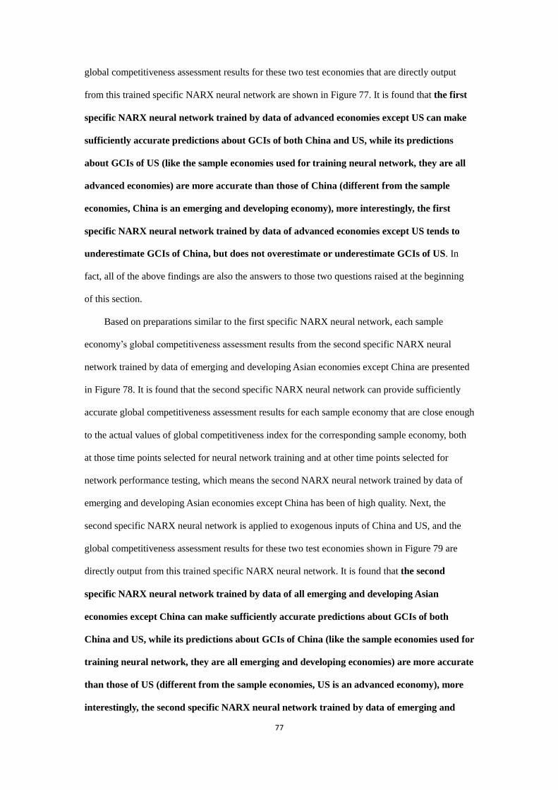
77

global competitiveness assessment results for these two test economies that are directly output

from this trained specific NARX neural network are shown in Figure 77. It is found that the first

specific NARX neural network trained by data of advanced economies except US can make

sufficiently accurate predictions about GCIs of both China and US, while its predictions

about GCIs of US (like the sample economies used for training neural network, they are all

advanced economies) are more accurate than those of China (different from the sample

economies, China is an emerging and developing economy), more interestingly, the first

specific NARX neural network trained by data of advanced economies except US tends to

underestimate GCIs of China, but does not overestimate or underestimate GCIs of US. In

fact, all of the above findings are also the answers to those two questions raised at the beginning

of this section.

Based on preparations similar to the first specific NARX neural network, each sample

economy’s global competitiveness assessment results from the second specific NARX neural

network trained by data of emerging and developing Asian economies except China are presented

in Figure 78. It is found that the second specific NARX neural network can provide sufficiently

accurate global competitiveness assessment results for each sample economy that are close enough

to the actual values of global competitiveness index for the corresponding sample economy, both

at those time points selected for neural network training and at other time points selected for

network performance testing, which means the second NARX neural network trained by data of

emerging and developing Asian economies except China has been of high quality. Next, the

second specific NARX neural network is applied to exogenous inputs of China and US, and the

global competitiveness assessment results for these two test economies shown in Figure 79 are

directly output from this trained specific NARX neural network. It is found that the second

specific NARX neural network trained by data of all emerging and developing Asian

economies except China can make sufficiently accurate predictions about GCIs of both

China and US, while its predictions about GCIs of China (like the sample economies used for

training neural network, they are all emerging and developing economies) are more accurate

than those of US (different from the sample economies, US is an advanced economy), more

interestingly, the second specific NARX neural network trained by data of emerging and

78

developing Asian economies except China tends to slightly overestimate GCIs of China,

while significantly underestimate GCIs of US. Then the two questions raised at the beginning of

this section are answered by the above findings.

Since most of the findings about the third specific NARX neural network are similar to those

of the previous two specific NARX neural networks, we are going to briefly discuss these findings

as follows. It is found from Figure 80 that the third specific NARX neural network trained by data

of European Union 28 economies and emerging & developing European economies can provide

sufficiently accurate global competitiveness assessment results for each sample economy that are

close enough to the actual values of global competitiveness index for the corresponding sample

economy, both at those time points selected for neural network training and at other time points

selected for network performance testing, which means the third NARX neural network after

training has already been of high quality. It is found in Figure 81 that the third specific NARX

neural network trained by data of both European Union 28 economies and emerging &

developing European economies can make sufficiently accurate predictions about GCIs of

both China and US, while its predictions about GCIs of China (like the emerging &

developing European economies used for training neural network, they are all emerging and

developing economies) are as accurate as those of US (like most of the European Union 28

economies used for training neural network, they are all advanced economies), more

interestingly, the third specific NARX neural network trained by data of both European

Union 28 economies and emerging & developing European economies usually tends to

slightly overestimate GCIs of China, while slightly underestimate GCIs of US. Then the two

questions raised at the beginning of this section are answered by the above findings again.

As a summary of the comparative case study on Global Competitiveness Index (GCI), we can

answer the two questions raised at the beginning of this section with enough certainty now: the

specific NARX neural network trained on the basis of the GCI related data of some

economies are usually capable of making sufficiently accurate predictions about GCIs of

other economies, as long as the number of sample economies used for training neural

network is large enough and the amount of relevant, systematic and comprehensive

information provided by their exogenous inputs is sufficiently large; the specific NARX

79

neural network trained on the basis of the data of some type of economies usually can give

more accurate predictions about GCIs of the same type of economies than those of different

type of economies, as long as the differences between the two types of economies reflected in

the indicators contained in their exogenous inputs are obvious and large enough, such as the

differences between advanced economies and emerging & developing economies.

7. Policy Recommendation

Unlike the human brain which is usually only capable of extracting information from a small

number of statistics, and integrating these information inefficiently, unsteadily and unrepeatably to

help improve the prediction of the object of interest, the NARX neural network specially

constructed for the prediction of the object of interest has the following advantages over the

human brain.

1. A NARX neural network has the potential to efficiently and effectively capture the

dynamics of almost arbitrary nonlinear dynamic system, since it has been proved in the

literature that any multi-dimensional nonlinear mapping of any continuous function can

be carried out by a two-layer NARX neural network (one hidden layer and one output

layer) with a suitable chosen number of neurons in its hidden layer, as a result, the ability

of the NARX neural network to construct almost arbitrary nonlinear dynamic mapping,

which takes complex multiple exogenous inputs and past values of the object of interest

as independent variables and gives the predictions of the object of interest as dependent

variables, is usually much higher than that of human brain.

2. During training, a NARX neural network is capable of automatically and efficiently

extracting useful information from not only past values of the time series of both the

object of interest and exogenous inputs (treated as independent variables), but also current

values of the time series of the object of interest waiting to be fitted (treated as dependent

variables), and also capable of automatically and adaptively building reasonable rules

between these complex multiple independent variables and dependent variables, through

the so called self-learning process, therefore, the fast self-learning ability of the NARX

neural network during training is usually much higher than that of human brain.

80

3. A NARX neural network is good at discovering long-term dependencies between past

values of both complex multiple exogenous inputs and the object of interest and current or

even future values of the object of interest, in other words, when the gap between the time

point where the relevant information appears and the time point where it is needed

becomes extremely large, a reasonably constructed NARX neural network is still able to

learn to connect the past information to the later output values over an extremely long

period of time, which seems as if this NARX neural network has far greater capacity of

long-term memory, and far more powerful ability of memory retrieval and memory

connection construction than the average human brain.

4. The generalization ability of the specially constructed NARX neural network is usually

much higher than that of human brain, in other words, the specially constructed NARX

neural network is better at applying those reasonable rules mentioned above between

complex multiple independent variables and dependent variables to new independent

variables with unseen background and meaning, and sometimes even with unknown data

accuracy and noise pollution, than the average human brain.

5. The fault tolerance ability of the specially constructed NARX neural network could be

better or at least as good as that of human brain, to be more specific, even if a small

number of hidden neurons in the hidden layer of a NARX neural network are damaged,

for example the weights in these hidden neurons that are updated through the self-learning

process are lost, the self-learning outcome of this NARX neural network after training can

usually still be maintained, and its prediction performance is usually not significantly

affected.

Of course, the application of the NARX neural network is still immature under some

scenarios due to there are no good and general decision criteria for the setting of the architecture

of the trained NARX neural network that affects its prediction performance. The most favorable

behavior of a specially constructed NARX model is dependent upon the exogenously designated

time delay that is especially important for the initial prediction, the selection of time points for

training, validation, or testing that may lead to either different fitting performance for the known

objects during training or different prediction performance for unknown objects outside of training,

81

and the selection of number of hidden neurons in the hidden layer of this NARX neural network,

which may result in the inadequate ability of the NARX neural network to construct highly

nonlinear dynamic mapping when this number is too small, on the contrary, could bring about not

only a real danger of overtraining the data and producing the false fitting of the known objects

during training that does not lead to better forecasts for unknown objects outside of training, but

also the excessively low training efficiency under the constraints of existing software and

hardware resources, when this number is too large. In general, the determination of these

architectural elements, in an optimal way, is a critical and difficult task for the construction of a

specific NARX neural network, which has no fixed criteria and needs to be determined based on

the specific requirements under the particular scenario.

In this study, the successful application of specific NARX neural networks in

macroeconomic forecasting, national goal setting and global competitiveness assessment

demonstrate that the above five advantages of the specially constructed NARX neural

networks over the human brain are obvious under the above three application scenarios,

while all architectural elements of these specific NARX neural networks can be simply and

directly determined as occasion demands. As a consequence, it’s strongly recommended that

government authorities and policy research institutions gradually turn to applying fully

trained NARX neural networks that are assessed as qualified to assist or even replace the

deductive and inductive abilities of the human brain in the macroeconomic forecasting tasks

and the market or industry segmentation forecasting tasks, in the tasks for setting national

or regional goals and market or industry targets, also in those tasks focusing on the global or

regional or national comparative assessments of the general performance of individuals or

the performance of individuals on particular subjects such as policy implementation and

government governance.

8. Conclusion

Although the trove of economic big data released by statistical agencies, private and public

surveys, and other sources is parsed every day by governments and authorities, economists and

market analysts, mostly for the purposes of economic forecasting, the full use of the trove of

82

economic big data through current econometric approaches and other modeling methods is not

that easy. However, with the rapid development of neural network methods and their cross-field

applications in recent years, certain types of neural networks may be considered as a general

method of making full use of the trove of economic data to make predictions.

After selecting the Nonlinear Autoregressive with Exogenous Input (NARX) neural network

as the method of this study through systematic and comprehensive literature review, and

constructing specific NARX neural networks under specific application scenarios involving

macroeconomic forecasting, national goal setting and global competitiveness assessment, this

study can concentrate on analyzing how different settings for exogenous inputs from the trove of

economic big data affect the prediction performance of NARX neural networks.

The case study on China demonstrates that the forecast target related abundant and

comprehensive exogenous inputs, which provide the sufficient amount of and the sufficiently

relevant, systematic and comprehensive information for the forecasts of the corresponding

macroeconomic or financial indicators, can further improve the prediction performance of

the specific NARX neural networks, compared with the forecast target related limited and

partial exogenous inputs.

The case study on US mainly demonstrates that the large set of exogenous inputs covering

all major aspects of a country’s macro economy helps to make the prediction performance of

the specific NARX neural network for forecasting a certain macroeconomic indicator or

index of that country much better than a small set of exogenous inputs closely related only to

that macroeconomic indicator or index.

The case study on Eurozone argues that not only those whole area related exogenous

inputs, but also those subdivision area related exogenous inputs can provide relevant,

systematic and comprehensive information for the forecasts of major macroeconomic

indicators and indices of the whole area, then using both whole area and subdivision area

related exogenous inputs can help to make the prediction performance of the specific NARX

neural network for forecasting a certain macroeconomic indicator or index of the whole area

much better than only adopting those whole area related exogenous inputs.

In the case study on Russia, it is found that only a small number of major and

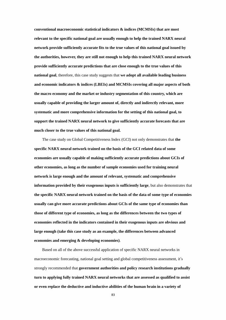
83

conventional macroeconomic statistical indicators & indices (MCMSIs) that are most

relevant to the specific national goal are usually enough to help the trained NARX neural

network provide sufficiently accurate fits to the true values of this national goal issued by

the authorities, however, they are still not enough to help this trained NARX neural network

provide sufficiently accurate predictions that are close enough to the true values of this

national goal, therefore, this case study suggests that we adopt all available leading business

and economic indicators & indices (LBEIs) and MCMSIs covering all major aspects of both

the macro economy and the market or industry segmentation of this country, which are

usually capable of providing the larger amount of, directly and indirectly relevant, more

systematic and more comprehensive information for the setting of this national goal, to

support the trained NARX neural network to give sufficiently accurate forecasts that are

much closer to the true values of this national goal.

The case study on Global Competitiveness Index (GCI) not only demonstrates that the

specific NARX neural network trained on the basis of the GCI related data of some

economies are usually capable of making sufficiently accurate predictions about GCIs of

other economies, as long as the number of sample economies used for training neural

network is large enough and the amount of relevant, systematic and comprehensive

information provided by their exogenous inputs is sufficiently large, but also demonstrates that

the specific NARX neural network trained on the basis of the data of some type of economies

usually can give more accurate predictions about GCIs of the same type of economies than

those of different type of economies, as long as the differences between the two types of

economies reflected in the indicators contained in their exogenous inputs are obvious and

large enough (take this case study as an example, the differences between advanced

economies and emerging & developing economies).

Based on all of the above successful application of specific NARX neural networks in

macroeconomic forecasting, national goal setting and global competitiveness assessment, it’s

strongly recommended that government authorities and policy research institutions gradually

turn to applying fully trained NARX neural networks that are assessed as qualified to assist

or even replace the deductive and inductive abilities of the human brain in a variety of

84

appropriate tasks, such as the macroeconomic forecasting tasks and the market or industry

segmentation forecasting tasks, the tasks for setting national or regional goals and market or

industry targets, and those tasks focusing on the global or regional or national comparative

assessments of the general performance of individuals or the performance of individuals on

particular subjects such as policy implementation and government governance.

85

References

1. Abdella, M., & Marwala, T. (2005). The use of genetic algorithms and neural networks to

approximate missing data in database. Computing and Informatics, 24, 207–212.

2. Aggarwal, S. K., Saini, L. M., & Kumar, A. (2009). Electricity price forecasting in

deregulated markets: A review and evaluation. International Journal of Electrical Power &

Energy Systems, 31(1), 13–22.

3. Anderson, R. N., Boulanger, A., Powell, W. B., & Scott, W. (2011). Adaptive stochastic

control for the smart grid. Proceedings of the IEEE, 99(6), 1098–1115.

4. Ardakani, F., & Ardehali, M. (2014). Long-term electrical energy consumption forecasting

for developing and developed economies based on different optimized models and historical

data types. Energy, 65, 452–461.

5. Asgari, H. (2014). Modelling, Simulation and control of gas turbines using artificial neural

networks. PhD thesis, Mechanical Engineering University of Canterbury Christchurch, New

Zealand.

6. Athey, S. (2017). Beyond prediction: using big data for policy problems. Science, 355(6324),

483–485.

7. Athey, S., & Imbens, G. W. (2017). The State of Applied Econometrics: Causality and Policy

Evaluation. Journal of Economic Perspectives, 31(2), 3–32.

8. Athey, S., & Imbens, G. W. (2019). Machine Learning Methods That Economists Should

Know About. Annual Review of Economics, 11(1), 685–725.

9. Azadeh, A., Asadzadeh, S., & Ghanbari, A. (2010). An adaptive network-based fuzzy

inference system for short-term natural gas demand estimation: uncertain and complex

environments. Energy Policy, 38(3), 1529–1536.

10. Azadeh, A., Ghaderi, S., & Sohrabkhani, S. (2008). A simulated-based neural network

algorithm for forecasting electrical energy consumption in Iran. Energy Policy, 36(7),

2637–2644.

11. Bandiera, O., Prat, A., Hansen, S., & Sadun, R. (2020). CEO Behavior and Firm Performance.

Journal of Political Economy, 128(4), 1325–1369.

12. Bassamzadeh, N., & Ghanem, R. (2017). Multiscale stochastic prediction of electricity

86

demand in smart grids using Bayesian networks. Applied Energy, 193, 369–380.

13. Beale, M. H., Hagan, M. T., & Demuth, H. B. (2014). Neural Network Toolbox™ User’s

Guide, R2014a ed. Natick, MA: The MathWorks.

14. Bento, P., Pombo, J., Calado, M., & Mariano, S. (2018). A bat optimized neural network and

wavelet transform approach for short-term price forecasting. Applied Energy, 210, 88–97.

15. Bok, B., Caratelli, D., Giannone, D., Sbordone, A. M., & Tambalotti, A. (2017).

Macroeconomic Nowcasting and Forecasting with Big Data. Federal Reserve Bank of New

York, Staff Report No 830.

16. Čeperić, E., Žiković, S., & Čeperić, V. (2017). Short-term forecasting of natural gas prices

using machine learning and feature selection algorithms. Energy, 140, 893–900.

17. Chalfin, A., Danieli, O., Hillis, A., Jelveh, Z., Luca, M., Ludwig, J., & Mullainathan, S.

(2016). Productivity and selection of human capital with machine learning. American

Economic Review, 106(5), 124–127.

18. Chen, N., Ribeiro, B., & Chen, A. (2015). Financial credit risk assessment: a recent review.

Artificial Intelligence Review, 45(1), 1–23.

19. Cheng, F., Fan, T., Fan, D., & Li, S. (2018). The prediction of oil price turning points with

log-periodic power law and multi-population genetic algorithm. Energy Economics, 72,

341–355.

20. Conejo, A. J., Contreras, J., Espinola, R., & Plazas, M. A. (2005). Forecasting electricity

prices for a day-ahead pool-based electric energy market. International journal of forecasting,

21(3), 435–462.

21. Cybenko, G. (1989). Approximation by superpositions of a sigmoidal function. Mathematics

of Control, Signals, and Systems, 2(4), 303–314.

22. Dagoumas, A. S., Koltsaklis, N. E., & Panapakidis, I. P. (2017). An integrated model for risk

management in electricity trade. Energy, 124, 350–363.

23. Debnath, K. B., & Mourshed, M. (2018). Forecasting methods in energy planning models.

Renewable and Sustainable Energy Reviews, 88, 297–325.

24. Ding, Y. (2018). A novel decompose-ensemble methodology with AIC-ANN approach for

crude oil forecasting. Energy, 154, 328–336.

87

25. Dudek, G. (2016). Multilayer perceptron for GEFCom2014 probabilistic electricity price

forecasting. International Journal of Forecasting, 32(3), 1057–1060.

26. Erel, I., Stern, L. H., Tan, C., & Weisbach, M. S. (2018). Selecting directors using machine

learning. European Corporate Governance Institute (ECGI), Finance Working Paper No.

605/2019. Available at https://ssrn.com/abstract=3144080 or

http://dx.doi.org/10.2139/ssrn.3144080

27. Ermis, K., Midilli, A., Dincer, I., & Rosen, M. (2007). Artificial neural network analysis of

world green energy use. Energy Policy, 35(3), 1731–1743.

28. Eugen, H. (2012). NARX neural networks for sequence processing tasks. Master of Science

Thesis, Universitat Politècnica de Catalunya – Universitat Rovira i Virgili – Universitat de

Barcelona.

29. Fan, X., Li, S., & Tian, L. (2015). Chaotic characteristic identification for carbon price and an

multi-layer perceptron network prediction model. Expert Systems with Applications, 42(8),

3945–3952.

30. Fan, Y., & Yu, S. (2015). Port container throughput forecast based on NARX neural network.

Journal of Shanghai Maritime University, 36(4), 1–5.

31. Fang, G., Tian, L., Fu, M., & Sun, M. (2013). The impacts of carbon tax on energy intensity

and economic growth–a dynamic evolution analysis on the case of China. Applied Energy,

110, 17–28.

32. Farajzadeh, Z., & Nematollahi, M. A. (2018). Energy intensity and its components in Iran:

Determinants and trends. Energy Economics, 73, 161–177.

33. Fethi, M. D., & Pasiouras, F. (2010). Assessing bank efficiency and performance with

operational research and artificial intelligence techniques: a survey. European Journal of

Operational Research, 204(2), 189–198.

34. Geem, Z. W. (2011). Transport energy demand modeling of South Korea using artificial

neural network. Energy policy, 39(8), 4644–4650.

35. Ghoddusi, H., Creamer, G. G., & Rafizadeh, N. (2019). Machine learning in energy

economics and finance: a review. Energy Economics, 81(6), 709–727.

36. Godarzi, A. A., Amiri, R. M., Talaei, A., & Jamasb, T. (2014). Predicting oil price movements:

88

A dynamic Artificial Neural Network approach. Energy Policy, 68, 371–382.

37. Guzman, S. M., Paz, J. O., & Tagert, M. L. M. (2017). The use of NARX neural networks to

forecast daily groundwater levels. Water Resources Management, 31, 1591–1603.

38. Handel, B., & Kolstad, J. (2017). Wearable Technologies and Health Behaviors: New Data

and New Methods to Understand Population Health. American Economic Review, 107(5),

481–485.

39. Hatcher, W. G., & Yu, W. (2018). A Survey of Deep Learning: Platforms, Applications and

Emerging Research Trends. IEEE Access, 6, 24411–24432.

40. Hu, X., Zhao, G., & Zhao, J. (2008). Forecasting model of coal demand based on matlab bp

neural network. Chinese Journal of Management Science, 10(16), 521–525.

41. Hu, Y., Liu, K., Zhang, X., Su, L., Ngai, E.W.T., & Liu, M. (2015). Application of

evolutionary computation for rule discovery in stock algorithmic trading: A literature review.

Applied Soft Computing, 36, 534–551.

42. Huang, L., & Wang, J. (2018). Global crude oil price prediction and synchronization based

accuracy evaluation using random wavelet neural network. Energy, 151, 875–888.

43. Islam, M. P., & Morimoto, T. (2015). Performance Prediction of Solar Collector Adsorber

Tube Temperature using a Nonlinear Autoregressive Model with eXogenous Input.

International Journal of Computer Applications, 114(12), 24–32.

44. Jammazi, R., & Aloui, C. (2012). Crude oil price forecasting: Experimental evidence from

wavelet decomposition and neural network modeling. Energy Economics, 34(3), 828–841.

45. Kasy, M. (2018). Optimal taxation and insurance using machine learning-Sufficient statistics

and beyond. Journal of Public Economics, 167, 205–219.

46. Kaytez, F., Taplamacioglu, M. C., Cam, E., & Hardalac, F. (2015). Forecasting electricity

consumption: A comparison of regression analysis, neural networks and least squares support

vector machines. International Journal of Electrical Power & Energy Systems, 67, 431–438.

47. Kearney, C., & Liu, S. (2014). Textual sentiment in finance: a survey of methods and models.

International Review of Financial Analysis, 33(3), 171–185.

48. Kirkos, E., & Manolopoulos, Y. (2004). Data mining in finance and accounting: A review of

current research trends. Proceedings of the 1st International Conference on Enterprise

89

Systems and Accounting (ICESAcc), 63–78.

49. Kirkos, E., Spathis, C., & Manolopoulos, Y. (2007). Data mining techniques for the detection

of fraudulent financial statements. Expert Systems with Applications, 32(4), 995–1003.

50. Kleinberg, J., Lakkaraju, H., Leskovec, J., Ludwig, J., & Mullainathan, S. (2018). Human

decisions and machine predictions. Quarterly Journal of Economics, 133(1), 237–293.

51. Kleinberg, J., Ludwig, J., Mullainathan, S., & Obermeyer, Z. (2015). Prediction policy

problems. American Economic Review, 105(5), 491–495.

52. Kumar, B. S., & Ravi, V. (2016). A survey of the applications of text mining in financial

domain. Knowledge-Based Systems, 114, 128–147.

53. Kumar, P. R., & Ravi, V. (2007). Bankruptcy prediction in banks and firms via statistical and

intelligent techniques – a review. European Journal of Operational Research, 180(1), 1–28.

54. Lago, J., De Ridder, F., & De Schutter, B. (2018). Forecasting spot electricity prices: Deep

learning approaches and empirical comparison of traditional algorithms. Applied Energy, 221,

386–405.

55. Lahsasna, A., Ainon, R. N., & Wah, T. Y. (2010). Credit scoring models using soft computing

methods: a survey. International Arab Journal of Information Technology, 7(2), 115–123.

56. Lai, T., To, W. M., Lo, W., & Choy, Y. (2008). Modeling of electricity consumption in the

Asian gaming and tourism center—Macao SAR, People’s Republic of China. Energy, 33(5),

679–688.

57. LeCun, Y., Bengio, Y., & Hinton, G. (2015). Deep learning. Nature, 521(7553), 436.

58. Lee, C. C., & Sheridan, S. C. (2018). A new approach to modeling temperature-related

mortality: non-linear autoregressive models with exogenous input. Environmental Research,

164(7), 53–64.

59. Lee, C.C., Sheridan, S. C., Barnes, B. B., Hu, C., Pirhalla, D. E., Ransibrahmanakul, V., &

Shein, K. (2016). The development of a non-linear auto-regressive model with exogenous

input to model climate-water clarity relationships: reconstructing a historical water clarity

index for the coastal waters of the southeastern USA. Theoretical & Applied Climatology,

130, 557–569.

60. Li, B., & Hoi, S. C. H. (2012). Online Portfolio Selection: A Survey. ACM Computing

90

Surveys, 46(3), 1–33.

61. Li, F. (2011). Textual analysis of corporate disclosures: a survey of the literature. Journal of

Accounting Literature, 29, 1–40.

62. Limanond, T., Jomnonkwao, S., & Srikaew, A. (2011). Projection of future transport energy

demand of Thailand. Energy policy, 39(5), 2754–2763.

63. Lin, W. Y., Hu, Y. H., & Tsai, C. F. (2012). Machine learning in financial crisis prediction: a

survey. IEEE Transactions on Systems Man & Cybernetics, Part C, 42(4), 421–436.

64. Liu, N., Tang, Q., Zhang, J., Fan, W., & Liu, J. (2014). A hybrid forecasting model with

parameter optimization for short-term load forecasting of micro-grids. Applied Energy, 129,

336–345.

65. Liu, X., Moreno, B., & García, A. S. (2016). A grey neural network and input-output

combined forecasting model. Primary energy consumption forecasts in Spanish economic

sectors. Energy, 115, 1042–1054.

66. Loughran, T., & McDonald, B. (2016). Textual analysis in accounting and finance: A survey.

Journal of Accounting Research, 54(4), 1187–1230.

67. Mahmoud, M. A., & Alajmi, A. F. (2010). Quantitative assessment of energy conservation

due to public awareness campaigns using neural networks. Applied Energy, 87(1), 220–228.

68. Marqués, A. I., García, V., & Sánchez, J. S. (2013). A literature review on the application of

evolutionary computing to credit scoring. Journal of the Operational Research Society, 64(9),

1384–1399.

69. MathWorks. (2020). Shallow Neural Network Time-Series Prediction and Modeling.

Available at

https://www.mathworks.com/help/deeplearning/gs/neural-network-time-series-prediction-and

-modeling.html

70. McBride, L., & Nichols, A. (2016). Retooling Poverty Targeting Using Out-of-Sample

Validation and Machine Learning. The World Bank Economic Review, 32(3), 531–550.

71. Metaxiotis, K., & Liagkouras, K. (2012). Multiobjective evolutionary algorithms for portfolio

management: a comprehensive literature review. Expert Systems with Application, 39(14),

11685–11698.

91

72. Mitra, L., & Mitra, G. (2012). Applications of news analytics in finance: A review. In The

Handbook of News Analytics in Finance, 1–39, John Wiley & Sons, Ltd.

73. Mittal, M., Goyal, L. M., Sethi, J. K., & Hemanth, D. J. (2019). Monitoring the impact of

economic crisis on crime in India using machine learning. Computational Economics, 53(4),

1467–1485.

74. Mittermayer, M., & Knolmayer, G. F. (2006). Text mining systems for market response to

news: A survey. University of Bern, Institute for Information Systems, Working Paper No

184.

75. Moshiri, S., & Foroutan, F. (2006). Forecasting nonlinear crude oil futures prices. The Energy

Journal, 27(4), 81–95.

76. Murat, Y. S., & Ceylan, H. (2006). Use of artificial neural networks for transport energy

demand modeling. Energy policy, 34(17), 3165–3172.

77. Nelwamondo, F. V., Mohamed, S., & Marwala, T. (2007). Missing data: A comparison of

neural network and expectation maximization techniques. Current Science, 93(11),

1514–1521.

78. Ngai, E. W. T., Hu, Y., Wong, Y. H., Chen, Y., & Sun, X. (2011). The application of data

mining techniques in financial fraud detection: a classification framework and an academic

review of literature. Decision Support Systems, 50(3), 559–569.

79. Nguyen, H. T., & Nabney, I. T. (2010). Short-term electricity demand and gas price forecasts

using wavelet transforms and adaptive models. Energy, 35(9), 3674–3685.

80. Ning, Y. C. (2003). A superposition wavelet-neural network model of coal demand forecast.

Journal of China Coal Society, 1, 021.

81. Number23. (2019). Learning NARX (Nonlinear autoregressive with external input) neural

network. Available at https://blog.csdn.net/sinat_17306241/article/details/88664606

82. Olah, C. (2015). Understanding LSTM Networks. Available at

http://colah.github.io/posts/2015-08-Understanding-LSTMs/

83. Ozbayoglu, A. M., Gudelek, M. U., & Sezer, O. B. (2020). Deep learning for financial

applications: a survey. Available at https://arxiv.org/abs/2002.05786

84. Panapakidis, I. P., & Dagoumas, A. S. (2016). Day-ahead electricity price forecasting via the

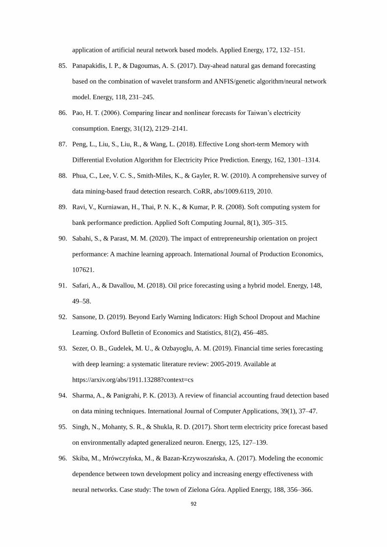
92

application of artificial neural network based models. Applied Energy, 172, 132–151.

85. Panapakidis, I. P., & Dagoumas, A. S. (2017). Day-ahead natural gas demand forecasting

based on the combination of wavelet transform and ANFIS/genetic algorithm/neural network

model. Energy, 118, 231–245.

86. Pao, H. T. (2006). Comparing linear and nonlinear forecasts for Taiwan’s electricity

consumption. Energy, 31(12), 2129–2141.

87. Peng, L., Liu, S., Liu, R., & Wang, L. (2018). Effective Long short-term Memory with

Differential Evolution Algorithm for Electricity Price Prediction. Energy, 162, 1301–1314.

88. Phua, C., Lee, V. C. S., Smith-Miles, K., & Gayler, R. W. (2010). A comprehensive survey of

data mining-based fraud detection research. CoRR, abs/1009.6119, 2010.

89. Ravi, V., Kurniawan, H., Thai, P. N. K., & Kumar, P. R. (2008). Soft computing system for

bank performance prediction. Applied Soft Computing Journal, 8(1), 305–315.

90. Sabahi, S., & Parast, M. M. (2020). The impact of entrepreneurship orientation on project

performance: A machine learning approach. International Journal of Production Economics,

107621.

91. Safari, A., & Davallou, M. (2018). Oil price forecasting using a hybrid model. Energy, 148,

49–58.

92. Sansone, D. (2019). Beyond Early Warning Indicators: High School Dropout and Machine

Learning. Oxford Bulletin of Economics and Statistics, 81(2), 456–485.

93. Sezer, O. B., Gudelek, M. U., & Ozbayoglu, A. M. (2019). Financial time series forecasting

with deep learning: a systematic literature review: 2005-2019. Available at

https://arxiv.org/abs/1911.13288?context=cs

94. Sharma, A., & Panigrahi, P. K. (2013). A review of financial accounting fraud detection based

on data mining techniques. International Journal of Computer Applications, 39(1), 37–47.

95. Singh, N., Mohanty, S. R., & Shukla, R. D. (2017). Short term electricity price forecast based

on environmentally adapted generalized neuron. Energy, 125, 127–139.

96. Skiba, M., Mrówczyńska, M., & Bazan-Krzywoszańska, A. (2017). Modeling the economic

dependence between town development policy and increasing energy effectiveness with

neural networks. Case study: The town of Zielona Góra. Applied Energy, 188, 356–366.

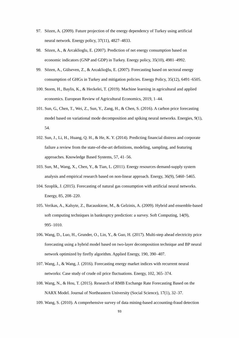
93

97. Sözen, A. (2009). Future projection of the energy dependency of Turkey using artificial

neural network. Energy policy, 37(11), 4827–4833.

98. Sözen, A., & Arcaklioglu, E. (2007). Prediction of net energy consumption based on

economic indicators (GNP and GDP) in Turkey. Energy policy, 35(10), 4981–4992.

99. Sözen, A., Gülseven, Z., & Arcaklioğlu, E. (2007). Forecasting based on sectoral energy

consumption of GHGs in Turkey and mitigation policies. Energy Policy, 35(12), 6491–6505.

100. Storm, H., Baylis, K., & Heckelei, T. (2019). Machine learning in agricultural and applied

economics. European Review of Agricultural Economics, 2019, 1–44.

101. Sun, G., Chen, T., Wei, Z., Sun, Y., Zang, H., & Chen, S. (2016). A carbon price forecasting

model based on variational mode decomposition and spiking neural networks. Energies, 9(1),

54.

102. Sun, J., Li, H., Huang, Q. H., & He, K. Y. (2014). Predicting financial distress and corporate

failure a review from the state-of-the-art definitions, modeling, sampling, and featuring

approaches. Knowledge Based Systems, 57, 41–56.

103. Sun, M., Wang, X., Chen, Y., & Tian, L. (2011). Energy resources demand-supply system

analysis and empirical research based on non-linear approach. Energy, 36(9), 5460–5465.

104. Szoplik, J. (2015). Forecasting of natural gas consumption with artificial neural networks.

Energy, 85, 208–220.

105. Verikas, A., Kalsyte, Z., Bacauskiene, M., & Gelzinis, A. (2009). Hybrid and ensemble-based

soft computing techniques in bankruptcy prediction: a survey. Soft Computing, 14(9),

995–1010.

106. Wang, D., Luo, H., Grunder, O., Lin, Y., & Guo, H. (2017). Multi-step ahead electricity price

forecasting using a hybrid model based on two-layer decomposition technique and BP neural

network optimized by firefly algorithm. Applied Energy, 190, 390–407.

107. Wang, J., & Wang, J. (2016). Forecasting energy market indices with recurrent neural

networks: Case study of crude oil price fluctuations. Energy, 102, 365–374.

108. Wang, N., & Hou, T. (2015). Research of RMB Exchange Rate Forecasting Based on the

NARX Model. Journal of Northeastern University (Social Science), 17(1), 32–37.

109. Wang, S. (2010). A comprehensive survey of data mining-based accounting-fraud detection

94

research. 2010 International Conference on Intelligent Computation Technology and

Automation, IEEE.

110. Weron, R. (2014). Electricity price forecasting: A review of the state-of-the-art with a look

into the future. International journal of forecasting, 30(4), 1030–1081.

111. West, J., & Bhattacharya, M. (2016). Intelligent financial fraud detection: a comprehensive

review. Computers & Security, 57, 47–66.

112. Wikipedia. (2019). Nonlinear autoregressive exogenous model. Available at

https://en.wikipedia.org/wiki/Nonlinear_autoregressive_exogenous_model

113. Xiao, J., Li, Y., Xie, L., Liu, D., & Huang, J. (2018). A hybrid model based on selective

ensemble for energy consumption forecasting in China. Energy, 159, 534–546.

114. Yang, J. H., Wu, C. Y., & Zhang, G. M. (2014). Coal demand prediction in Shandong

Province based on artificial firefly wavelet neural network. Advanced Materials Research,

962, 1931–1935.

115. Yang, Z., Ce, L., & Lian, L. (2017). Electricity price forecasting by a hybrid model,

combining wavelet transform, ARMA and kernel-based extreme learning machine methods.

Applied Energy, 190, 291–305.

116. Yu, L., Wang, S., & Lai, K. K. (2008). Forecasting crude oil price with an EMD-based neural

network ensemble learning paradigm. Energy Economics, 30(5), 2623–2635.

117. Yu, L., Zhao, Y., & Tang, L. (2017). Ensemble forecasting for complex time series using

sparse representation and neural networks. Journal of Forecasting, 36(2), 122–138.

118. Yue, D., Wu, X., Wang, Y., Li, Y., & Chu, C. (2007). A review of data mining-based financial

fraud detection research. 2007 International Conference on Wireless Communications,

Networking and Mobile Computing, IEEE.

119. Zhang, W., Tian, L., Wang, M., Zhen, Z., & Fang, G. (2016). The evolution model of

electricity market on the stable development in China and its dynamic analysis. Energy, 114,

344–359.

120. Zhao, Y., Li, J., & Yu, L. (2017). A deep learning ensemble approach for crude oil price

forecasting. Energy Economics, 66, 9–16.

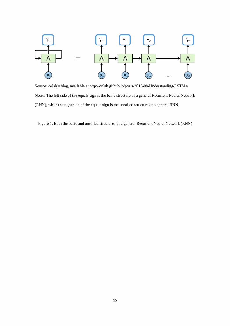
95

Source: colah’s blog, available at http://colah.github.io/posts/2015-08-Understanding-LSTMs/

Notes: The left side of the equals sign is the basic structure of a general Recurrent Neural Network

(RNN), while the right side of the equals sign is the unrolled structure of a general RNN.

Figure 1. Both the basic and unrolled structures of a general Recurrent Neural Network (RNN)

Yt Y0 Y1 Y2 Yt

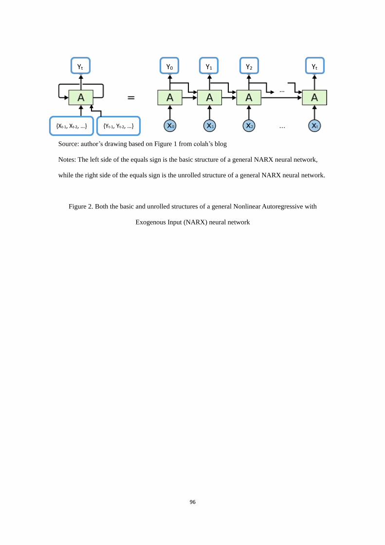
96

Source: author’s drawing based on Figure 1 from colah’s blog

Notes: The left side of the equals sign is the basic structure of a general NARX neural network,

while the right side of the equals sign is the unrolled structure of a general NARX neural network.

Figure 2. Both the basic and unrolled structures of a general Nonlinear Autoregressive with

Exogenous Input (NARX) neural network

Yt Y0 Y1 Y2 Yt

{Yt-1, Yt-2, …}

…

{Xt-1, Xt-2, …}

97

Source: Neural Net Time Series Toolbox of Matlab

Notes: The specific NARX neural network in the above figure is set to have 31 exogenous inputs

series {xt, xt-1,…}, 1 monthly frequency target series {yt, yt-1,…}, 2 hidden neurons in the hidden

layer, and 12-month or 1-year time delays for the dynamic forecasting of the target series.

Figure 3. Example of a specific NARX neural network for monthly frequency forecasting of the

target series

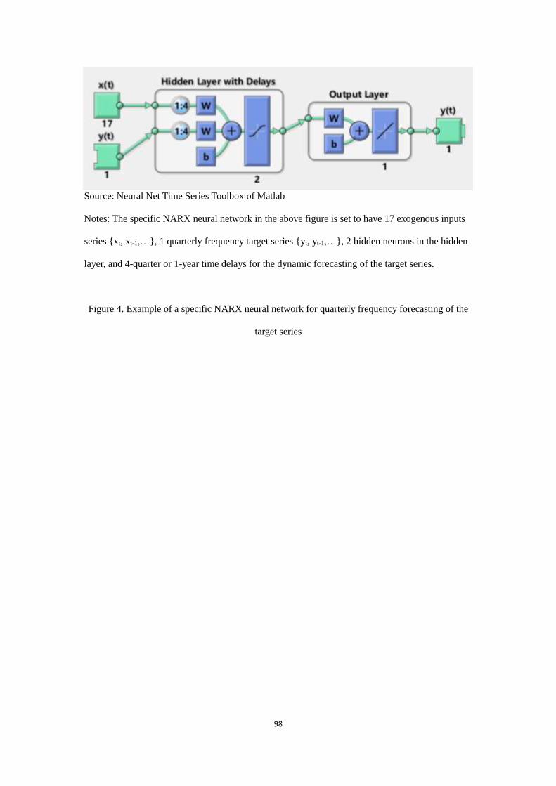
98

Source: Neural Net Time Series Toolbox of Matlab

Notes: The specific NARX neural network in the above figure is set to have 17 exogenous inputs

series {xt, xt-1,…}, 1 quarterly frequency target series {yt, yt-1,…}, 2 hidden neurons in the hidden

layer, and 4-quarter or 1-year time delays for the dynamic forecasting of the target series.

Figure 4. Example of a specific NARX neural network for quarterly frequency forecasting of the

target series

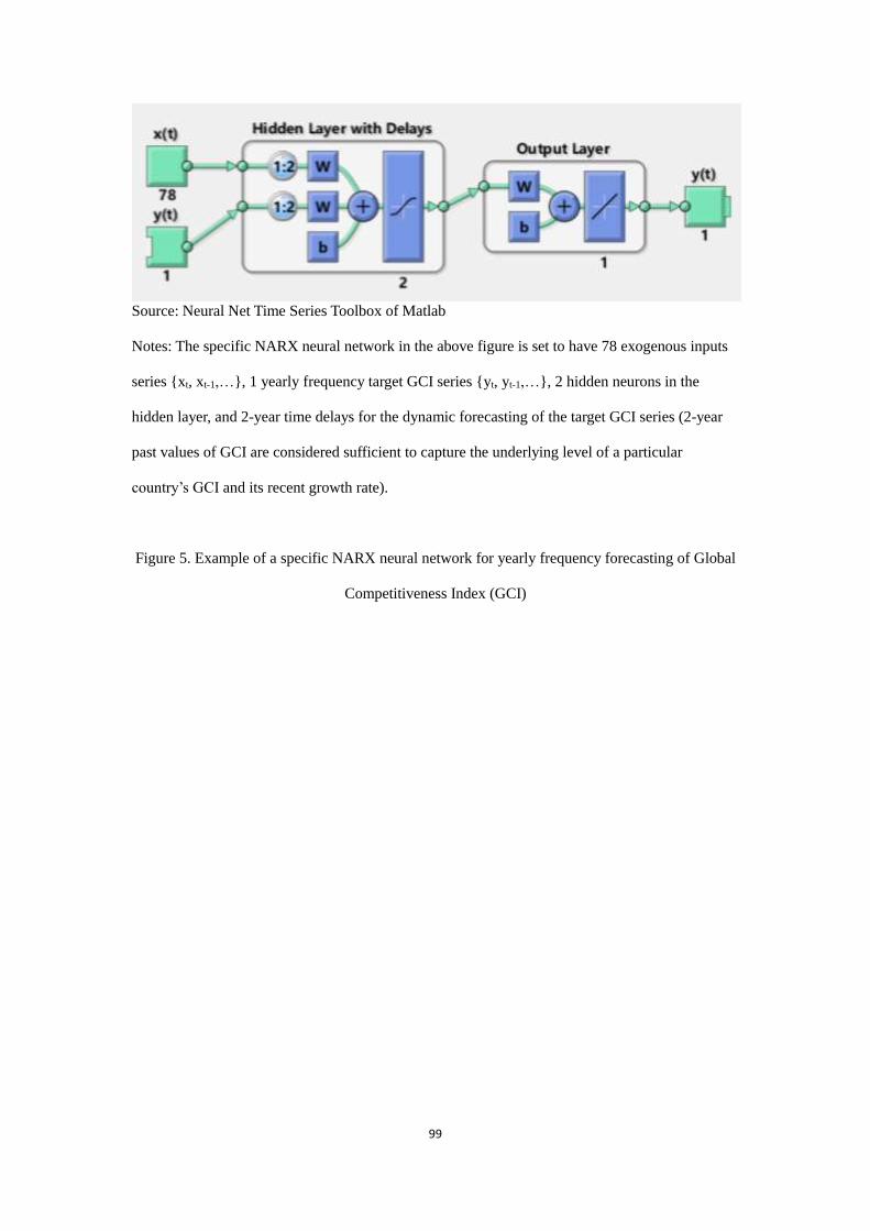
99

Source: Neural Net Time Series Toolbox of Matlab

Notes: The specific NARX neural network in the above figure is set to have 78 exogenous inputs

series {xt, xt-1,…}, 1 yearly frequency target GCI series {yt, yt-1,…}, 2 hidden neurons in the

hidden layer, and 2-year time delays for the dynamic forecasting of the target GCI series (2-year

past values of GCI are considered sufficient to capture the underlying level of a particular

country’s GCI and its recent growth rate).

Figure 5. Example of a specific NARX neural network for yearly frequency forecasting of Global

Competitiveness Index (GCI)

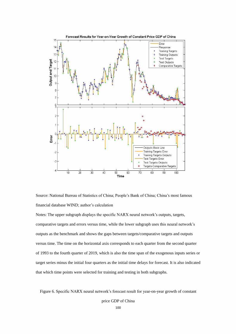
100

Source: National Bureau of Statistics of China; People’s Bank of China; China’s most famous

financial database WIND; author’s calculation

Notes: The upper subgraph displays the specific NARX neural network’s outputs, targets,

comparative targets and errors versus time, while the lower subgraph uses this neural network’s

outputs as the benchmark and shows the gaps between targets/comparative targets and outputs

versus time. The time on the horizontal axis corresponds to each quarter from the second quarter

of 1993 to the fourth quarter of 2019, which is also the time span of the exogenous inputs series or

target series minus the initial four quarters as the initial time delays for forecast. It is also indicated

that which time points were selected for training and testing in both subgraphs.

Figure 6. Specific NARX neural network’s forecast result for year-on-year growth of constant

price GDP of China

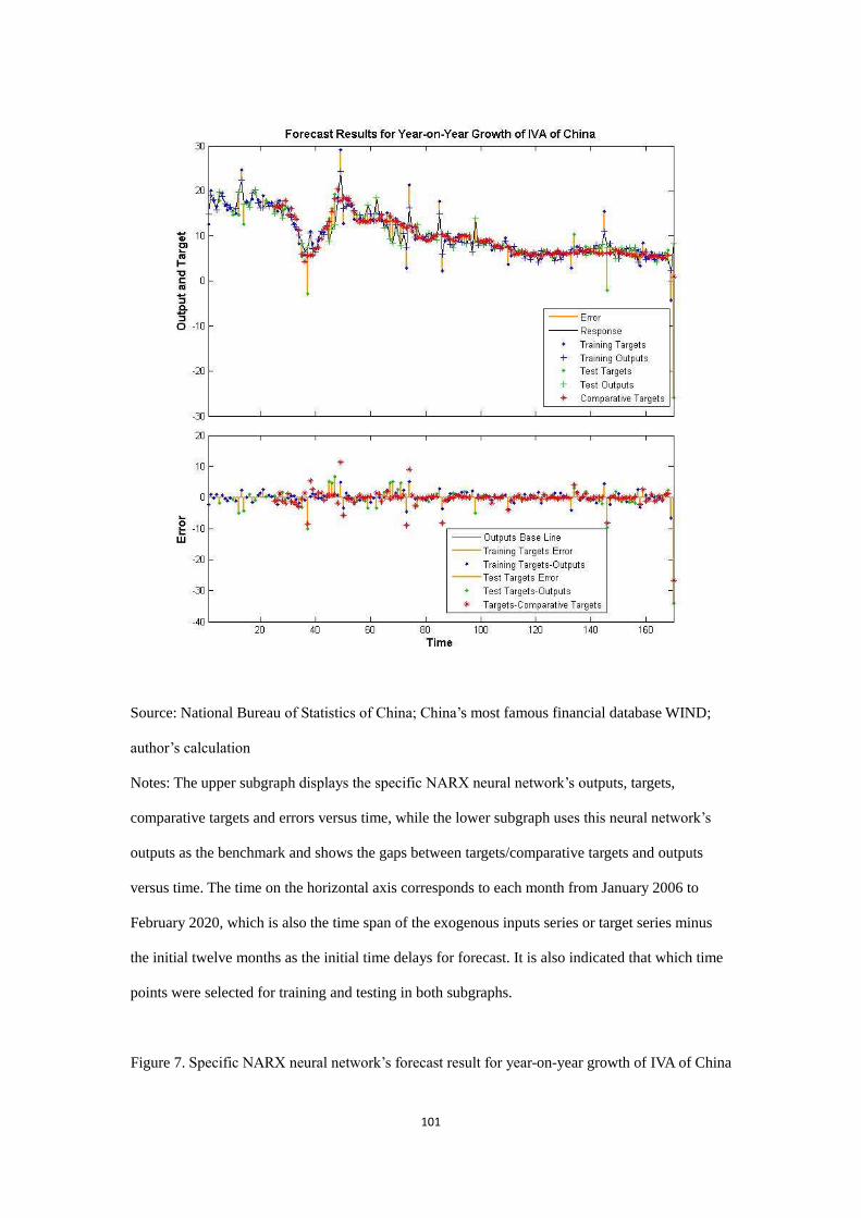
101

Source: National Bureau of Statistics of China; China’s most famous financial database WIND;

author’s calculation

Notes: The upper subgraph displays the specific NARX neural network’s outputs, targets,

comparative targets and errors versus time, while the lower subgraph uses this neural network’s

outputs as the benchmark and shows the gaps between targets/comparative targets and outputs

versus time. The time on the horizontal axis corresponds to each month from January 2006 to

February 2020, which is also the time span of the exogenous inputs series or target series minus

the initial twelve months as the initial time delays for forecast. It is also indicated that which time

points were selected for training and testing in both subgraphs.

Figure 7. Specific NARX neural network’s forecast result for year-on-year growth of IVA of China

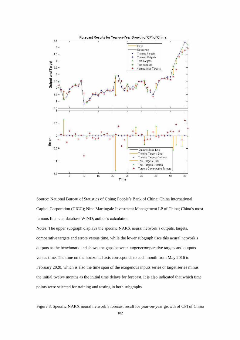
102

Source: National Bureau of Statistics of China; People’s Bank of China; China International

Capital Corporation (CICC); Nine Martingale Investment Management LP of China; China’s most

famous financial database WIND; author’s calculation

Notes: The upper subgraph displays the specific NARX neural network’s outputs, targets,

comparative targets and errors versus time, while the lower subgraph uses this neural network’s

outputs as the benchmark and shows the gaps between targets/comparative targets and outputs

versus time. The time on the horizontal axis corresponds to each month from May 2016 to

February 2020, which is also the time span of the exogenous inputs series or target series minus

the initial twelve months as the initial time delays for forecast. It is also indicated that which time

points were selected for training and testing in both subgraphs.

Figure 8. Specific NARX neural network’s forecast result for year-on-year growth of CPI of China

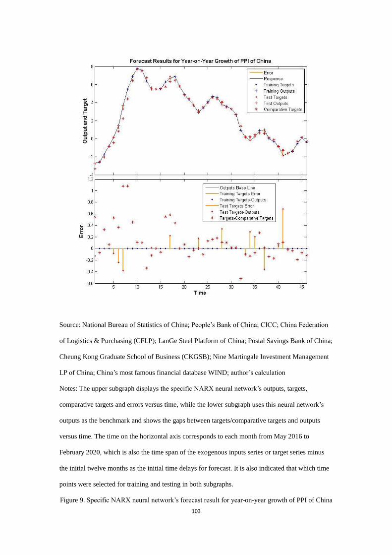
103

Source: National Bureau of Statistics of China; People’s Bank of China; CICC; China Federation

of Logistics & Purchasing (CFLP); LanGe Steel Platform of China; Postal Savings Bank of China;

Cheung Kong Graduate School of Business (CKGSB); Nine Martingale Investment Management

LP of China; China’s most famous financial database WIND; author’s calculation

Notes: The upper subgraph displays the specific NARX neural network’s outputs, targets,

comparative targets and errors versus time, while the lower subgraph uses this neural network’s

outputs as the benchmark and shows the gaps between targets/comparative targets and outputs

versus time. The time on the horizontal axis corresponds to each month from May 2016 to

February 2020, which is also the time span of the exogenous inputs series or target series minus

the initial twelve months as the initial time delays for forecast. It is also indicated that which time

points were selected for training and testing in both subgraphs.

Figure 9. Specific NARX neural network’s forecast result for year-on-year growth of PPI of China

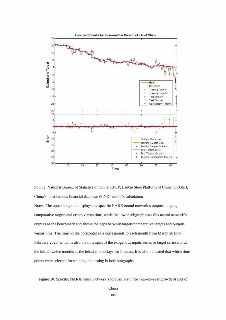
104

Source: National Bureau of Statistics of China; CFLP; LanGe Steel Platform of China; CKGSB;

China’s most famous financial database WIND; author’s calculation

Notes: The upper subgraph displays the specific NARX neural network’s outputs, targets,

comparative targets and errors versus time, while the lower subgraph uses this neural network’s

outputs as the benchmark and shows the gaps between targets/comparative targets and outputs

versus time. The time on the horizontal axis corresponds to each month from March 2013 to

February 2020, which is also the time span of the exogenous inputs series or target series minus

the initial twelve months as the initial time delays for forecast. It is also indicated that which time

points were selected for training and testing in both subgraphs.

Figure 10. Specific NARX neural network’s forecast result for year-on-year growth of FAI of

China

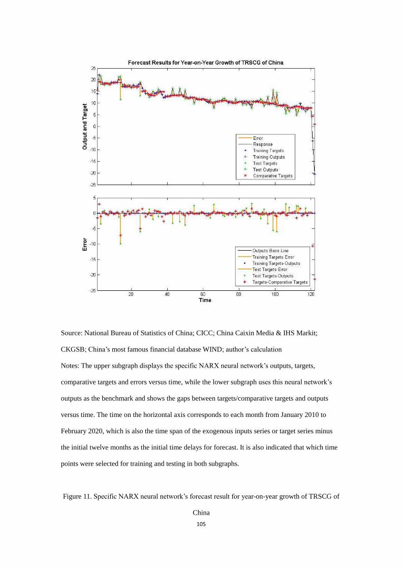
105

Source: National Bureau of Statistics of China; CICC; China Caixin Media & IHS Markit;

CKGSB; China’s most famous financial database WIND; author’s calculation

Notes: The upper subgraph displays the specific NARX neural network’s outputs, targets,

comparative targets and errors versus time, while the lower subgraph uses this neural network’s

outputs as the benchmark and shows the gaps between targets/comparative targets and outputs

versus time. The time on the horizontal axis corresponds to each month from January 2010 to

February 2020, which is also the time span of the exogenous inputs series or target series minus

the initial twelve months as the initial time delays for forecast. It is also indicated that which time

points were selected for training and testing in both subgraphs.

Figure 11. Specific NARX neural network’s forecast result for year-on-year growth of TRSCG of

China

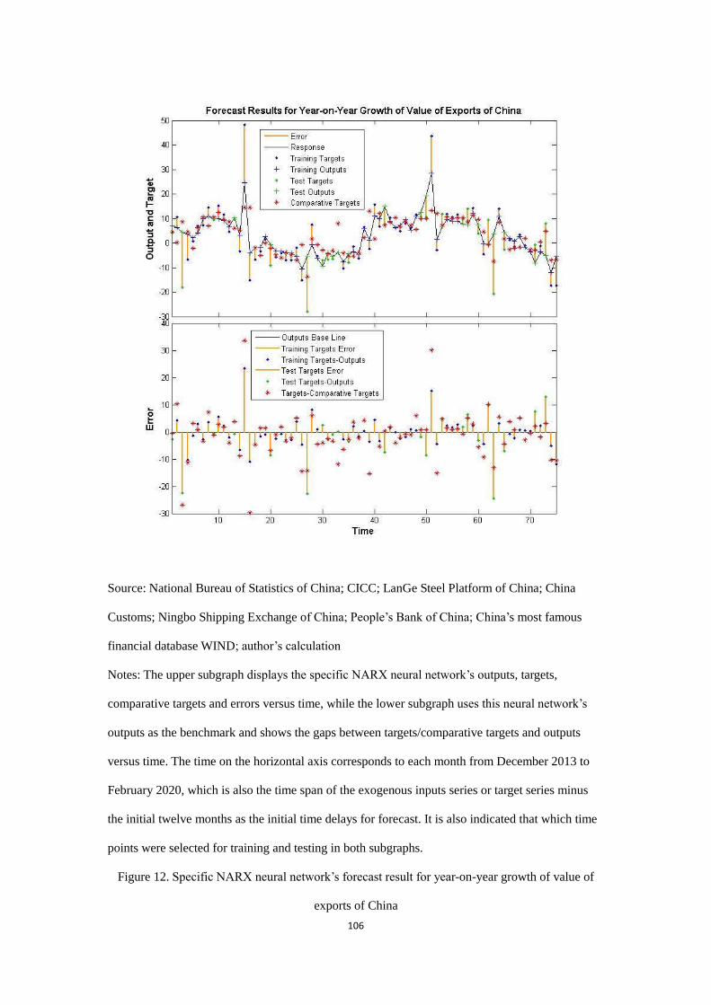
106

Source: National Bureau of Statistics of China; CICC; LanGe Steel Platform of China; China

Customs; Ningbo Shipping Exchange of China; People’s Bank of China; China’s most famous

financial database WIND; author’s calculation

Notes: The upper subgraph displays the specific NARX neural network’s outputs, targets,

comparative targets and errors versus time, while the lower subgraph uses this neural network’s

outputs as the benchmark and shows the gaps between targets/comparative targets and outputs

versus time. The time on the horizontal axis corresponds to each month from December 2013 to

February 2020, which is also the time span of the exogenous inputs series or target series minus

the initial twelve months as the initial time delays for forecast. It is also indicated that which time

points were selected for training and testing in both subgraphs.

Figure 12. Specific NARX neural network’s forecast result for year-on-year growth of value of

exports of China

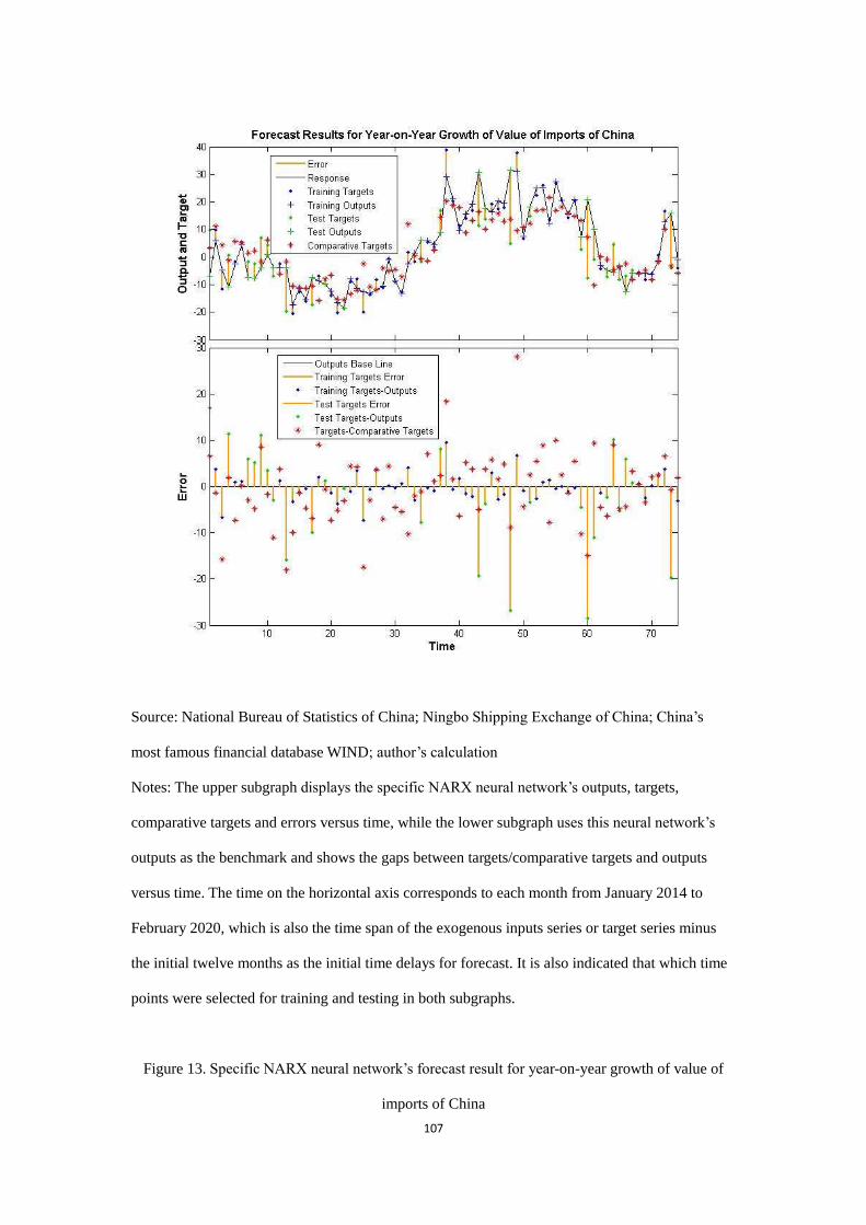
107

Source: National Bureau of Statistics of China; Ningbo Shipping Exchange of China; China’s

most famous financial database WIND; author’s calculation

Notes: The upper subgraph displays the specific NARX neural network’s outputs, targets,

comparative targets and errors versus time, while the lower subgraph uses this neural network’s

outputs as the benchmark and shows the gaps between targets/comparative targets and outputs

versus time. The time on the horizontal axis corresponds to each month from January 2014 to

February 2020, which is also the time span of the exogenous inputs series or target series minus

the initial twelve months as the initial time delays for forecast. It is also indicated that which time

points were selected for training and testing in both subgraphs.

Figure 13. Specific NARX neural network’s forecast result for year-on-year growth of value of

imports of China

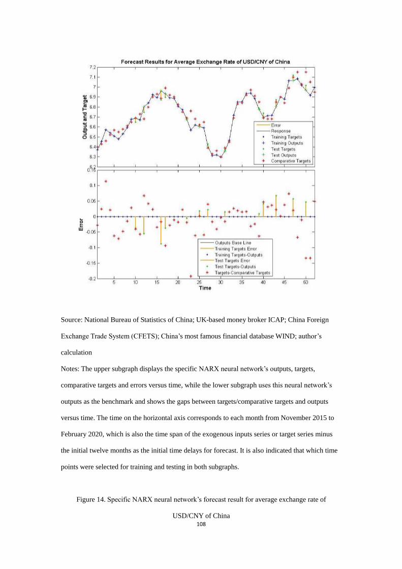
108

Source: National Bureau of Statistics of China; UK-based money broker ICAP; China Foreign

Exchange Trade System (CFETS); China’s most famous financial database WIND; author’s

calculation

Notes: The upper subgraph displays the specific NARX neural network’s outputs, targets,

comparative targets and errors versus time, while the lower subgraph uses this neural network’s

outputs as the benchmark and shows the gaps between targets/comparative targets and outputs

versus time. The time on the horizontal axis corresponds to each month from November 2015 to

February 2020, which is also the time span of the exogenous inputs series or target series minus

the initial twelve months as the initial time delays for forecast. It is also indicated that which time

points were selected for training and testing in both subgraphs.

Figure 14. Specific NARX neural network’s forecast result for average exchange rate of

USD/CNY of China

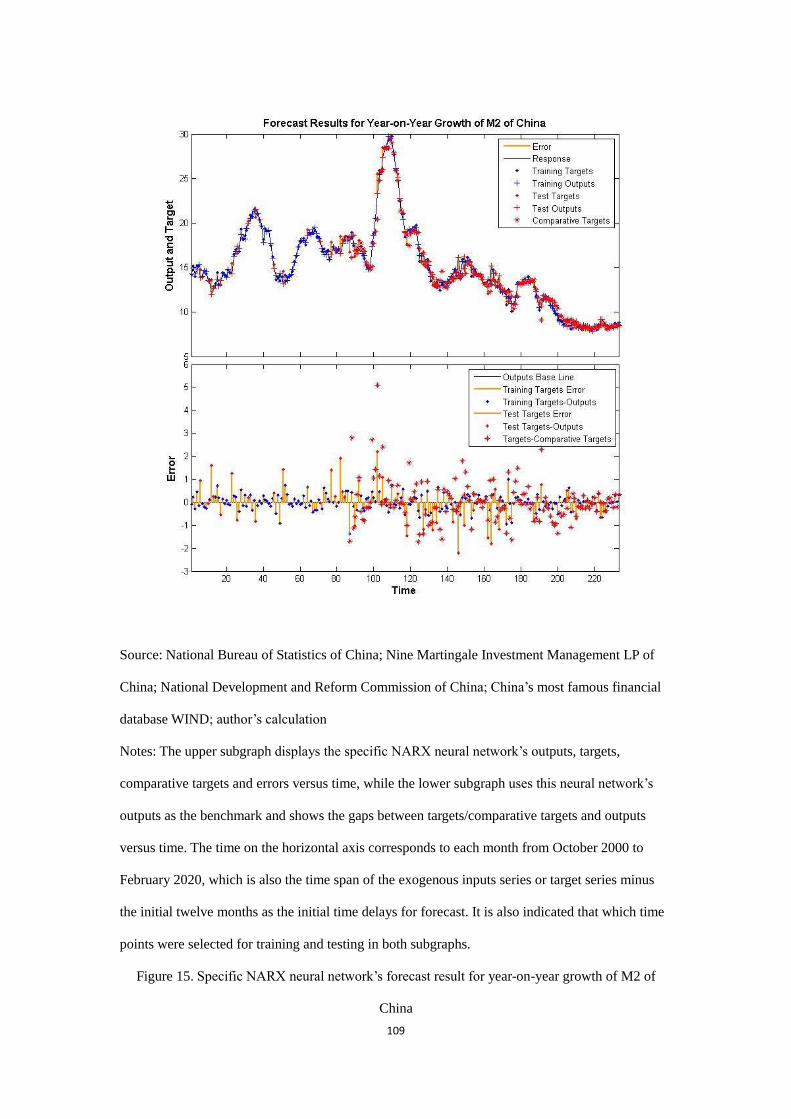
109

Source: National Bureau of Statistics of China; Nine Martingale Investment Management LP of

China; National Development and Reform Commission of China; China’s most famous financial

database WIND; author’s calculation

Notes: The upper subgraph displays the specific NARX neural network’s outputs, targets,

comparative targets and errors versus time, while the lower subgraph uses this neural network’s

outputs as the benchmark and shows the gaps between targets/comparative targets and outputs

versus time. The time on the horizontal axis corresponds to each month from October 2000 to

February 2020, which is also the time span of the exogenous inputs series or target series minus

the initial twelve months as the initial time delays for forecast. It is also indicated that which time

points were selected for training and testing in both subgraphs.

Figure 15. Specific NARX neural network’s forecast result for year-on-year growth of M2 of

China

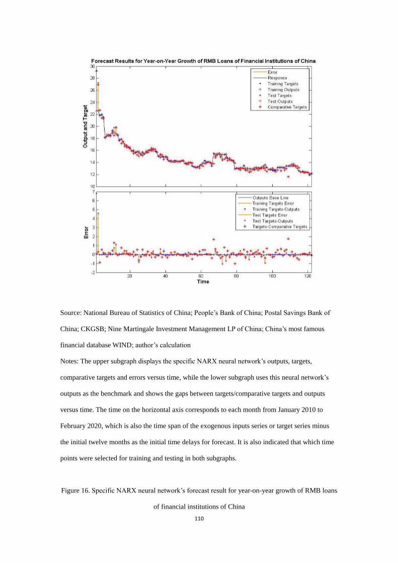
110

Source: National Bureau of Statistics of China; People’s Bank of China; Postal Savings Bank of

China; CKGSB; Nine Martingale Investment Management LP of China; China’s most famous

financial database WIND; author’s calculation

Notes: The upper subgraph displays the specific NARX neural network’s outputs, targets,

comparative targets and errors versus time, while the lower subgraph uses this neural network’s

outputs as the benchmark and shows the gaps between targets/comparative targets and outputs

versus time. The time on the horizontal axis corresponds to each month from January 2010 to

February 2020, which is also the time span of the exogenous inputs series or target series minus

the initial twelve months as the initial time delays for forecast. It is also indicated that which time

points were selected for training and testing in both subgraphs.

Figure 16. Specific NARX neural network’s forecast result for year-on-year growth of RMB loans

of financial institutions of China

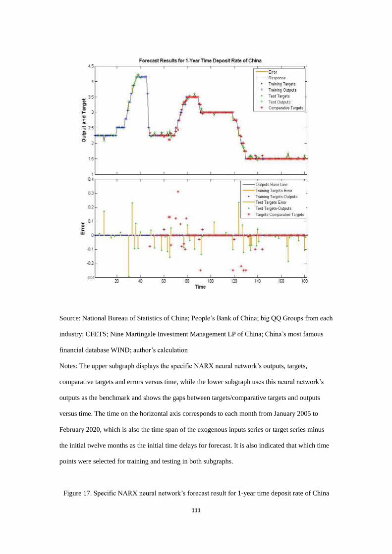
111

Source: National Bureau of Statistics of China; People’s Bank of China; big QQ Groups from each

industry; CFETS; Nine Martingale Investment Management LP of China; China’s most famous

financial database WIND; author’s calculation

Notes: The upper subgraph displays the specific NARX neural network’s outputs, targets,

comparative targets and errors versus time, while the lower subgraph uses this neural network’s

outputs as the benchmark and shows the gaps between targets/comparative targets and outputs

versus time. The time on the horizontal axis corresponds to each month from January 2005 to

February 2020, which is also the time span of the exogenous inputs series or target series minus

the initial twelve months as the initial time delays for forecast. It is also indicated that which time

points were selected for training and testing in both subgraphs.

Figure 17. Specific NARX neural network’s forecast result for 1-year time deposit rate of China

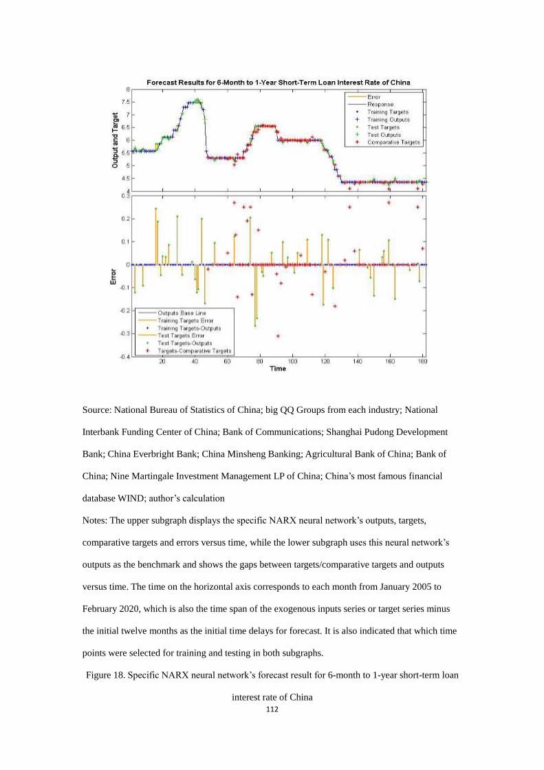
112

Source: National Bureau of Statistics of China; big QQ Groups from each industry; National

Interbank Funding Center of China; Bank of Communications; Shanghai Pudong Development

Bank; China Everbright Bank; China Minsheng Banking; Agricultural Bank of China; Bank of

China; Nine Martingale Investment Management LP of China; China’s most famous financial

database WIND; author’s calculation

Notes: The upper subgraph displays the specific NARX neural network’s outputs, targets,

comparative targets and errors versus time, while the lower subgraph uses this neural network’s

outputs as the benchmark and shows the gaps between targets/comparative targets and outputs

versus time. The time on the horizontal axis corresponds to each month from January 2005 to

February 2020, which is also the time span of the exogenous inputs series or target series minus

the initial twelve months as the initial time delays for forecast. It is also indicated that which time

points were selected for training and testing in both subgraphs.

Figure 18. Specific NARX neural network’s forecast result for 6-month to 1-year short-term loan

interest rate of China

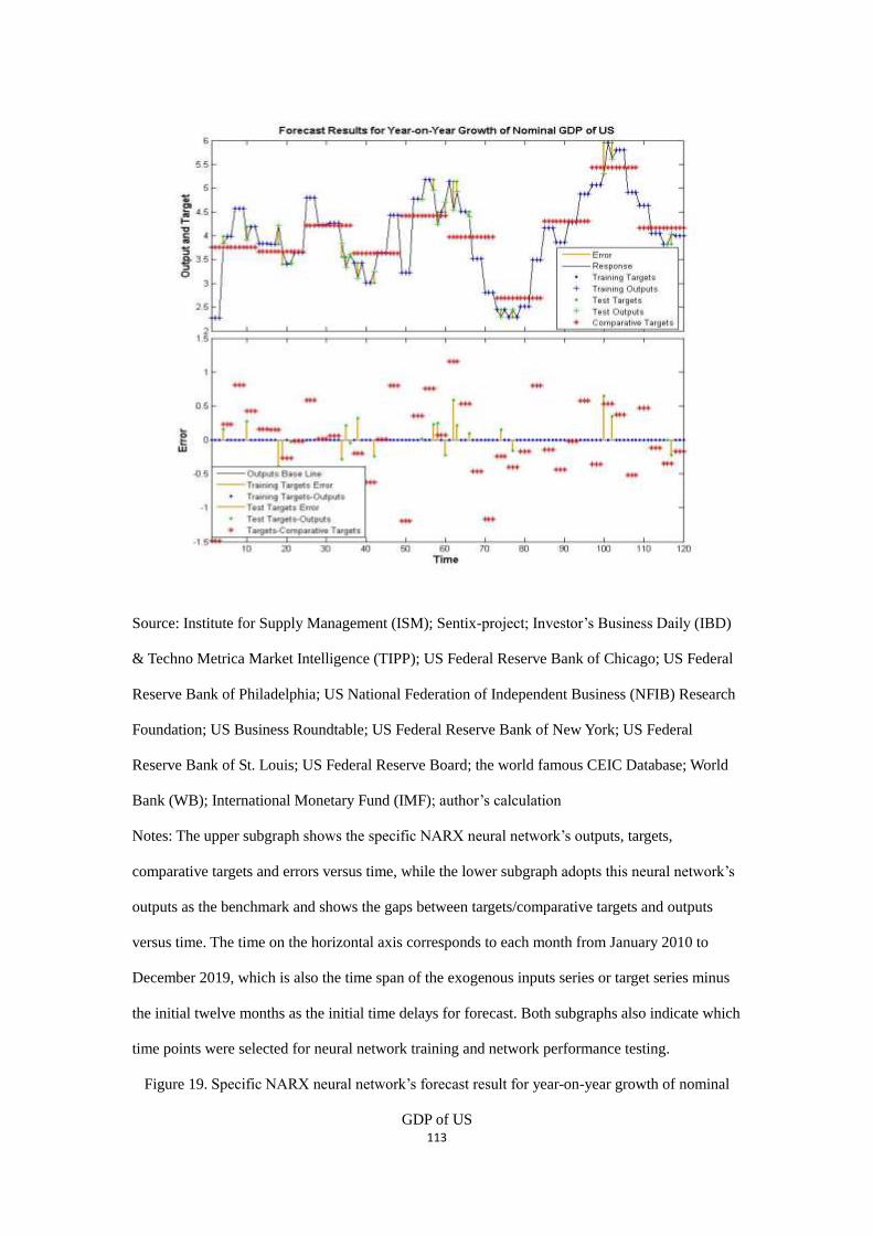
113

Source: Institute for Supply Management (ISM); Sentix-project; Investor’s Business Daily (IBD)

& Techno Metrica Market Intelligence (TIPP); US Federal Reserve Bank of Chicago; US Federal

Reserve Bank of Philadelphia; US National Federation of Independent Business (NFIB) Research

Foundation; US Business Roundtable; US Federal Reserve Bank of New York; US Federal

Reserve Bank of St. Louis; US Federal Reserve Board; the world famous CEIC Database; World

Bank (WB); International Monetary Fund (IMF); author’s calculation

Notes: The upper subgraph shows the specific NARX neural network’s outputs, targets,

comparative targets and errors versus time, while the lower subgraph adopts this neural network’s

outputs as the benchmark and shows the gaps between targets/comparative targets and outputs

versus time. The time on the horizontal axis corresponds to each month from January 2010 to

December 2019, which is also the time span of the exogenous inputs series or target series minus

the initial twelve months as the initial time delays for forecast. Both subgraphs also indicate which

time points were selected for neural network training and network performance testing.

Figure 19. Specific NARX neural network’s forecast result for year-on-year growth of nominal

GDP of US

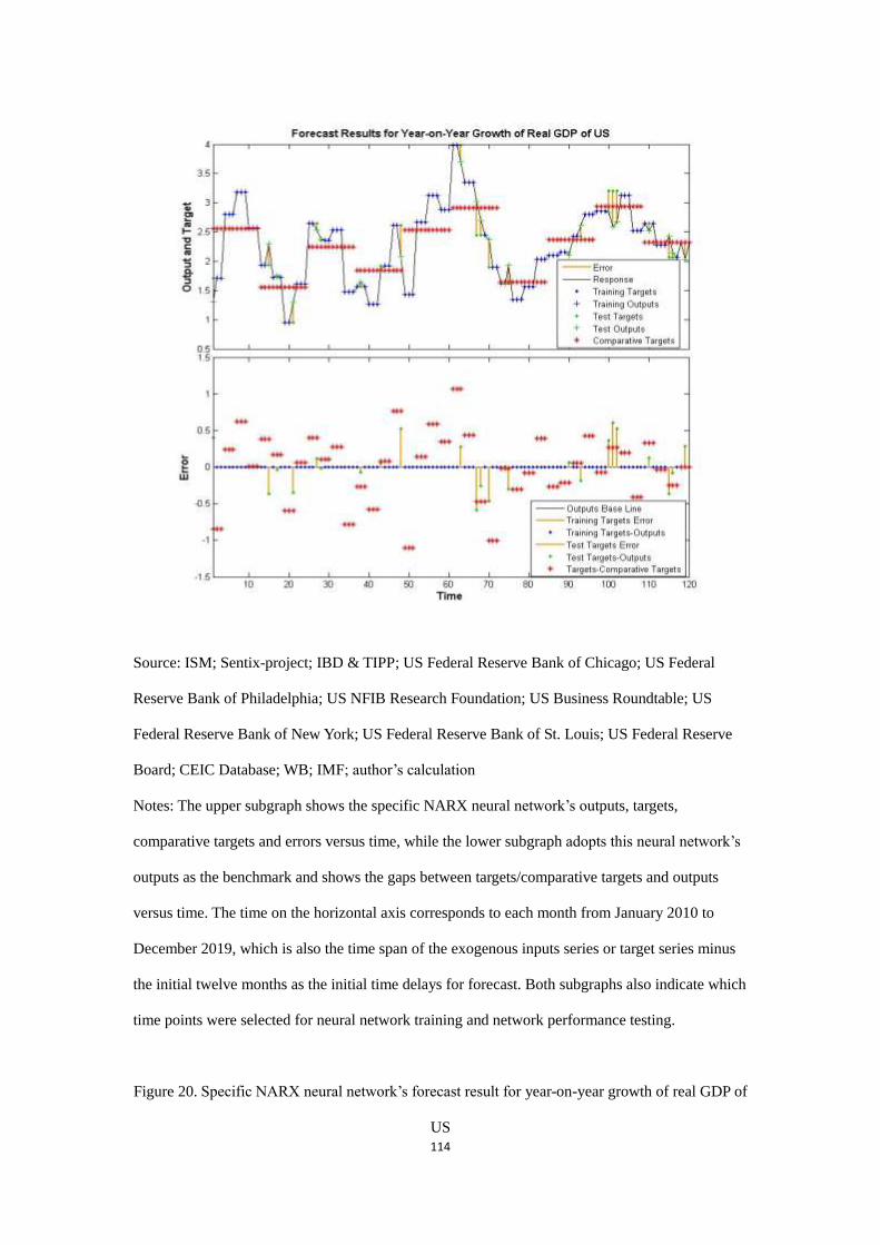
114

Source: ISM; Sentix-project; IBD & TIPP; US Federal Reserve Bank of Chicago; US Federal

Reserve Bank of Philadelphia; US NFIB Research Foundation; US Business Roundtable; US

Federal Reserve Bank of New York; US Federal Reserve Bank of St. Louis; US Federal Reserve

Board; CEIC Database; WB; IMF; author’s calculation

Notes: The upper subgraph shows the specific NARX neural network’s outputs, targets,

comparative targets and errors versus time, while the lower subgraph adopts this neural network’s

outputs as the benchmark and shows the gaps between targets/comparative targets and outputs

versus time. The time on the horizontal axis corresponds to each month from January 2010 to

December 2019, which is also the time span of the exogenous inputs series or target series minus

the initial twelve months as the initial time delays for forecast. Both subgraphs also indicate which

time points were selected for neural network training and network performance testing.

Figure 20. Specific NARX neural network’s forecast result for year-on-year growth of real GDP of

US

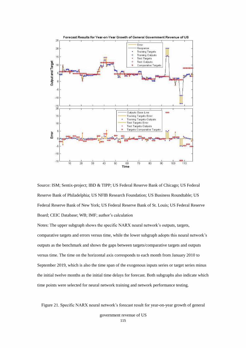
115

Source: ISM; Sentix-project; IBD & TIPP; US Federal Reserve Bank of Chicago; US Federal

Reserve Bank of Philadelphia; US NFIB Research Foundation; US Business Roundtable; US

Federal Reserve Bank of New York; US Federal Reserve Bank of St. Louis; US Federal Reserve

Board; CEIC Database; WB; IMF; author’s calculation

Notes: The upper subgraph shows the specific NARX neural network’s outputs, targets,

comparative targets and errors versus time, while the lower subgraph adopts this neural network’s

outputs as the benchmark and shows the gaps between targets/comparative targets and outputs

versus time. The time on the horizontal axis corresponds to each month from January 2010 to

September 2019, which is also the time span of the exogenous inputs series or target series minus

the initial twelve months as the initial time delays for forecast. Both subgraphs also indicate which

time points were selected for neural network training and network performance testing.

Figure 21. Specific NARX neural network’s forecast result for year-on-year growth of general

government revenue of US

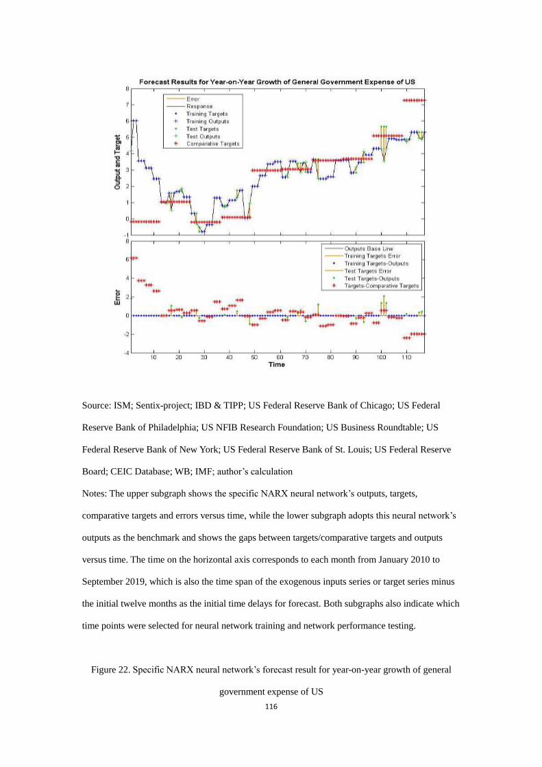
116

Source: ISM; Sentix-project; IBD & TIPP; US Federal Reserve Bank of Chicago; US Federal

Reserve Bank of Philadelphia; US NFIB Research Foundation; US Business Roundtable; US

Federal Reserve Bank of New York; US Federal Reserve Bank of St. Louis; US Federal Reserve

Board; CEIC Database; WB; IMF; author’s calculation

Notes: The upper subgraph shows the specific NARX neural network’s outputs, targets,

comparative targets and errors versus time, while the lower subgraph adopts this neural network’s

outputs as the benchmark and shows the gaps between targets/comparative targets and outputs

versus time. The time on the horizontal axis corresponds to each month from January 2010 to

September 2019, which is also the time span of the exogenous inputs series or target series minus

the initial twelve months as the initial time delays for forecast. Both subgraphs also indicate which

time points were selected for neural network training and network performance testing.

Figure 22. Specific NARX neural network’s forecast result for year-on-year growth of general

government expense of US

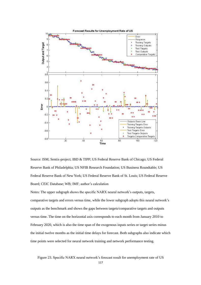
117

Source: ISM; Sentix-project; IBD & TIPP; US Federal Reserve Bank of Chicago; US Federal

Reserve Bank of Philadelphia; US NFIB Research Foundation; US Business Roundtable; US

Federal Reserve Bank of New York; US Federal Reserve Bank of St. Louis; US Federal Reserve

Board; CEIC Database; WB; IMF; author’s calculation

Notes: The upper subgraph shows the specific NARX neural network’s outputs, targets,

comparative targets and errors versus time, while the lower subgraph adopts this neural network’s

outputs as the benchmark and shows the gaps between targets/comparative targets and outputs

versus time. The time on the horizontal axis corresponds to each month from January 2010 to

February 2020, which is also the time span of the exogenous inputs series or target series minus

the initial twelve months as the initial time delays for forecast. Both subgraphs also indicate which

time points were selected for neural network training and network performance testing.

Figure 23. Specific NARX neural network’s forecast result for unemployment rate of US

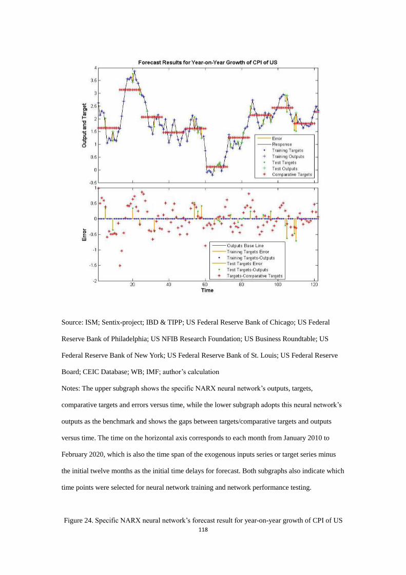
118

Source: ISM; Sentix-project; IBD & TIPP; US Federal Reserve Bank of Chicago; US Federal

Reserve Bank of Philadelphia; US NFIB Research Foundation; US Business Roundtable; US

Federal Reserve Bank of New York; US Federal Reserve Bank of St. Louis; US Federal Reserve

Board; CEIC Database; WB; IMF; author’s calculation

Notes: The upper subgraph shows the specific NARX neural network’s outputs, targets,

comparative targets and errors versus time, while the lower subgraph adopts this neural network’s

outputs as the benchmark and shows the gaps between targets/comparative targets and outputs

versus time. The time on the horizontal axis corresponds to each month from January 2010 to

February 2020, which is also the time span of the exogenous inputs series or target series minus

the initial twelve months as the initial time delays for forecast. Both subgraphs also indicate which

time points were selected for neural network training and network performance testing.

Figure 24. Specific NARX neural network’s forecast result for year-on-year growth of CPI of US

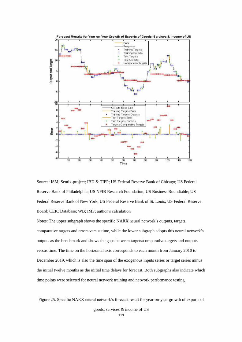
119

Source: ISM; Sentix-project; IBD & TIPP; US Federal Reserve Bank of Chicago; US Federal

Reserve Bank of Philadelphia; US NFIB Research Foundation; US Business Roundtable; US

Federal Reserve Bank of New York; US Federal Reserve Bank of St. Louis; US Federal Reserve

Board; CEIC Database; WB; IMF; author’s calculation

Notes: The upper subgraph shows the specific NARX neural network’s outputs, targets,

comparative targets and errors versus time, while the lower subgraph adopts this neural network’s

outputs as the benchmark and shows the gaps between targets/comparative targets and outputs

versus time. The time on the horizontal axis corresponds to each month from January 2010 to

December 2019, which is also the time span of the exogenous inputs series or target series minus

the initial twelve months as the initial time delays for forecast. Both subgraphs also indicate which

time points were selected for neural network training and network performance testing.

Figure 25. Specific NARX neural network’s forecast result for year-on-year growth of exports of

goods, services & income of US

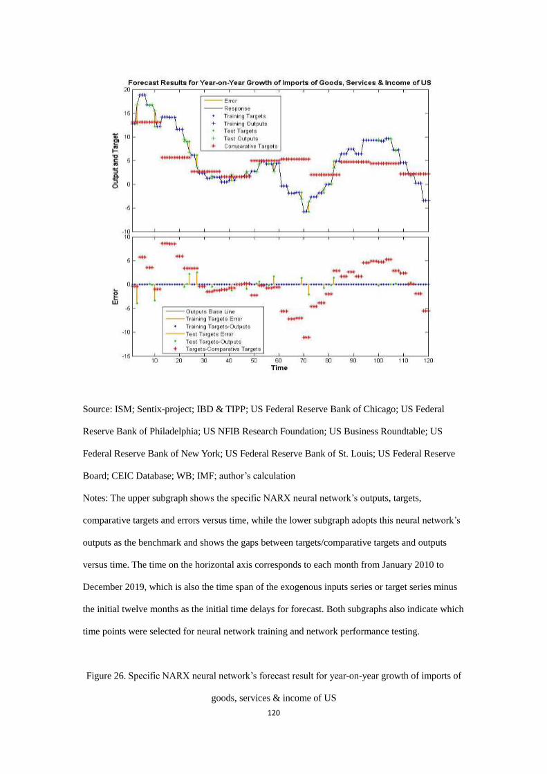
120

Source: ISM; Sentix-project; IBD & TIPP; US Federal Reserve Bank of Chicago; US Federal

Reserve Bank of Philadelphia; US NFIB Research Foundation; US Business Roundtable; US

Federal Reserve Bank of New York; US Federal Reserve Bank of St. Louis; US Federal Reserve

Board; CEIC Database; WB; IMF; author’s calculation

Notes: The upper subgraph shows the specific NARX neural network’s outputs, targets,

comparative targets and errors versus time, while the lower subgraph adopts this neural network’s

outputs as the benchmark and shows the gaps between targets/comparative targets and outputs

versus time. The time on the horizontal axis corresponds to each month from January 2010 to

December 2019, which is also the time span of the exogenous inputs series or target series minus

the initial twelve months as the initial time delays for forecast. Both subgraphs also indicate which

time points were selected for neural network training and network performance testing.

Figure 26. Specific NARX neural network’s forecast result for year-on-year growth of imports of

goods, services & income of US

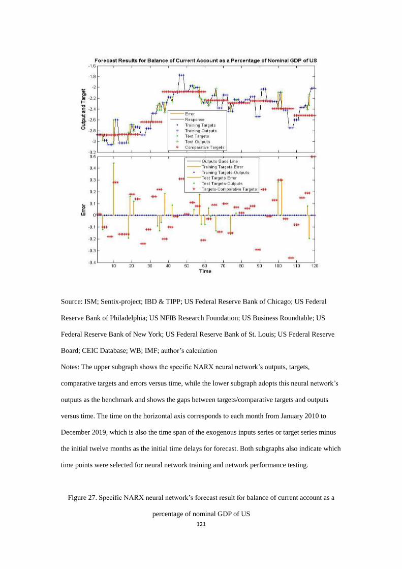
121

Source: ISM; Sentix-project; IBD & TIPP; US Federal Reserve Bank of Chicago; US Federal

Reserve Bank of Philadelphia; US NFIB Research Foundation; US Business Roundtable; US

Federal Reserve Bank of New York; US Federal Reserve Bank of St. Louis; US Federal Reserve

Board; CEIC Database; WB; IMF; author’s calculation

Notes: The upper subgraph shows the specific NARX neural network’s outputs, targets,

comparative targets and errors versus time, while the lower subgraph adopts this neural network’s

outputs as the benchmark and shows the gaps between targets/comparative targets and outputs

versus time. The time on the horizontal axis corresponds to each month from January 2010 to

December 2019, which is also the time span of the exogenous inputs series or target series minus

the initial twelve months as the initial time delays for forecast. Both subgraphs also indicate which

time points were selected for neural network training and network performance testing.

Figure 27. Specific NARX neural network’s forecast result for balance of current account as a

percentage of nominal GDP of US

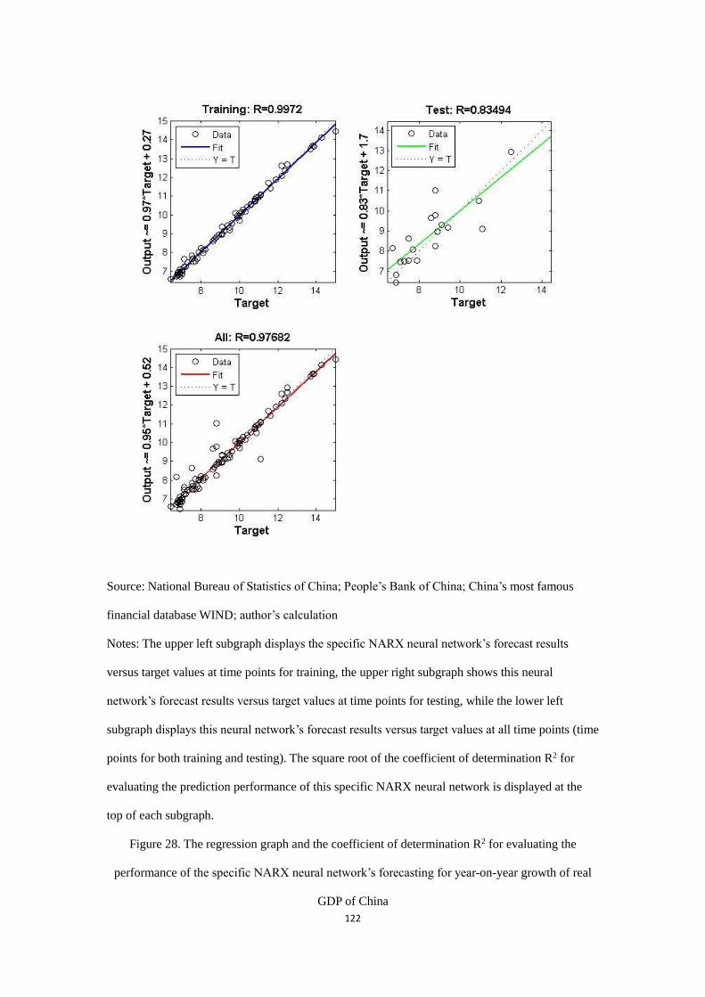
122

Source: National Bureau of Statistics of China; People’s Bank of China; China’s most famous

financial database WIND; author’s calculation

Notes: The upper left subgraph displays the specific NARX neural network’s forecast results

versus target values at time points for training, the upper right subgraph shows this neural

network’s forecast results versus target values at time points for testing, while the lower left

subgraph displays this neural network’s forecast results versus target values at all time points (time

points for both training and testing). The square root of the coefficient of determination R2 for

evaluating the prediction performance of this specific NARX neural network is displayed at the

top of each subgraph.

Figure 28. The regression graph and the coefficient of determination R2 for evaluating the

performance of the specific NARX neural network’s forecasting for year-on-year growth of real

GDP of China

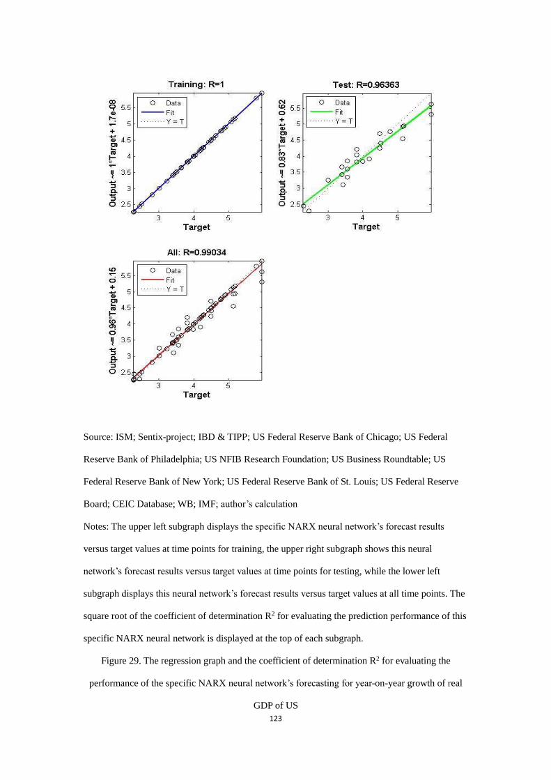
123

Source: ISM; Sentix-project; IBD & TIPP; US Federal Reserve Bank of Chicago; US Federal

Reserve Bank of Philadelphia; US NFIB Research Foundation; US Business Roundtable; US

Federal Reserve Bank of New York; US Federal Reserve Bank of St. Louis; US Federal Reserve

Board; CEIC Database; WB; IMF; author’s calculation

Notes: The upper left subgraph displays the specific NARX neural network’s forecast results

versus target values at time points for training, the upper right subgraph shows this neural

network’s forecast results versus target values at time points for testing, while the lower left

subgraph displays this neural network’s forecast results versus target values at all time points. The

square root of the coefficient of determination R2 for evaluating the prediction performance of this

specific NARX neural network is displayed at the top of each subgraph.

Figure 29. The regression graph and the coefficient of determination R2 for evaluating the

performance of the specific NARX neural network’s forecasting for year-on-year growth of real

GDP of US

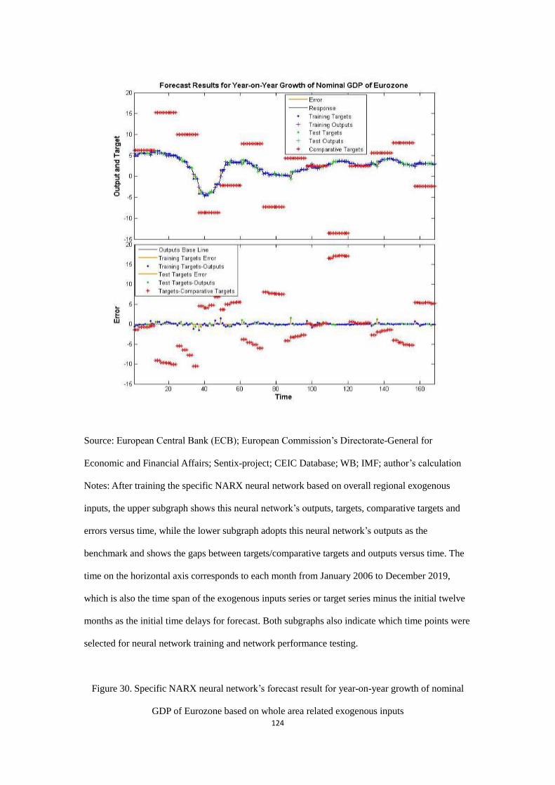
124

Source: European Central Bank (ECB); European Commission’s Directorate-General for

Economic and Financial Affairs; Sentix-project; CEIC Database; WB; IMF; author’s calculation

Notes: After training the specific NARX neural network based on overall regional exogenous

inputs, the upper subgraph shows this neural network’s outputs, targets, comparative targets and

errors versus time, while the lower subgraph adopts this neural network’s outputs as the

benchmark and shows the gaps between targets/comparative targets and outputs versus time. The

time on the horizontal axis corresponds to each month from January 2006 to December 2019,

which is also the time span of the exogenous inputs series or target series minus the initial twelve

months as the initial time delays for forecast. Both subgraphs also indicate which time points were

selected for neural network training and network performance testing.

Figure 30. Specific NARX neural network’s forecast result for year-on-year growth of nominal

GDP of Eurozone based on whole area related exogenous inputs

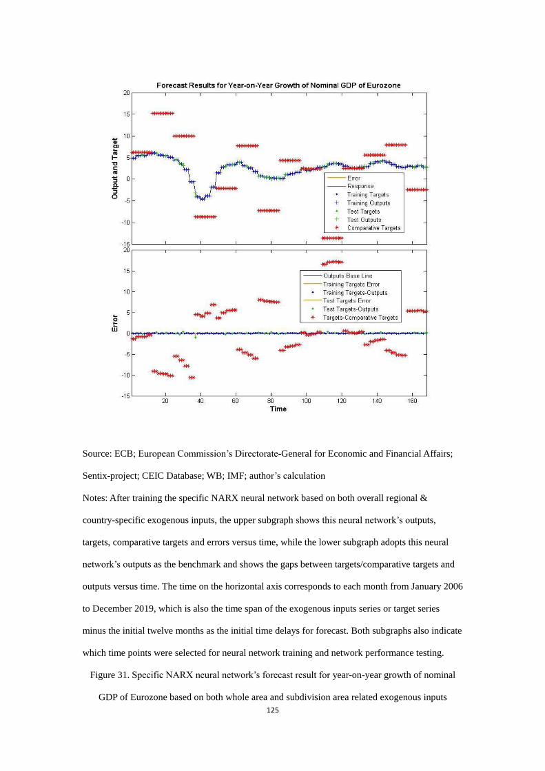
125

Source: ECB; European Commission’s Directorate-General for Economic and Financial Affairs;

Sentix-project; CEIC Database; WB; IMF; author’s calculation

Notes: After training the specific NARX neural network based on both overall regional &

country-specific exogenous inputs, the upper subgraph shows this neural network’s outputs,

targets, comparative targets and errors versus time, while the lower subgraph adopts this neural

network’s outputs as the benchmark and shows the gaps between targets/comparative targets and

outputs versus time. The time on the horizontal axis corresponds to each month from January 2006

to December 2019, which is also the time span of the exogenous inputs series or target series

minus the initial twelve months as the initial time delays for forecast. Both subgraphs also indicate

which time points were selected for neural network training and network performance testing.

Figure 31. Specific NARX neural network’s forecast result for year-on-year growth of nominal

GDP of Eurozone based on both whole area and subdivision area related exogenous inputs

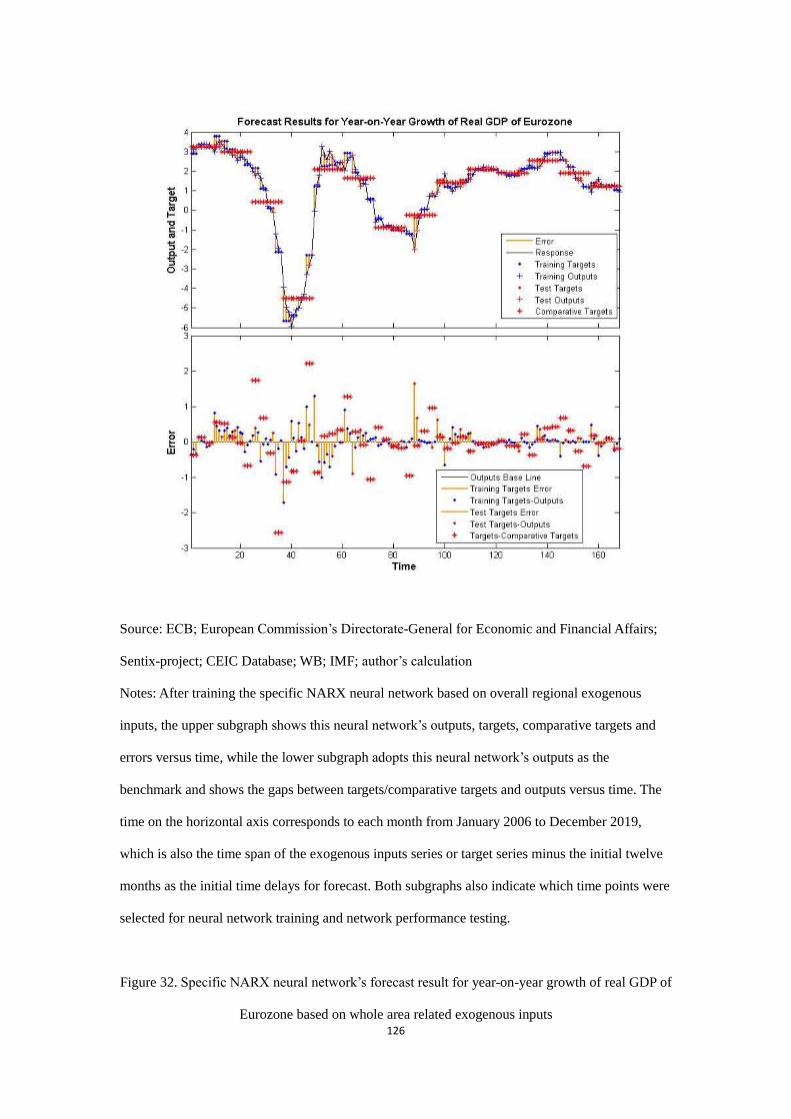
126

Source: ECB; European Commission’s Directorate-General for Economic and Financial Affairs;

Sentix-project; CEIC Database; WB; IMF; author’s calculation

Notes: After training the specific NARX neural network based on overall regional exogenous

inputs, the upper subgraph shows this neural network’s outputs, targets, comparative targets and

errors versus time, while the lower subgraph adopts this neural network’s outputs as the

benchmark and shows the gaps between targets/comparative targets and outputs versus time. The

time on the horizontal axis corresponds to each month from January 2006 to December 2019,

which is also the time span of the exogenous inputs series or target series minus the initial twelve

months as the initial time delays for forecast. Both subgraphs also indicate which time points were

selected for neural network training and network performance testing.

Figure 32. Specific NARX neural network’s forecast result for year-on-year growth of real GDP of

Eurozone based on whole area related exogenous inputs

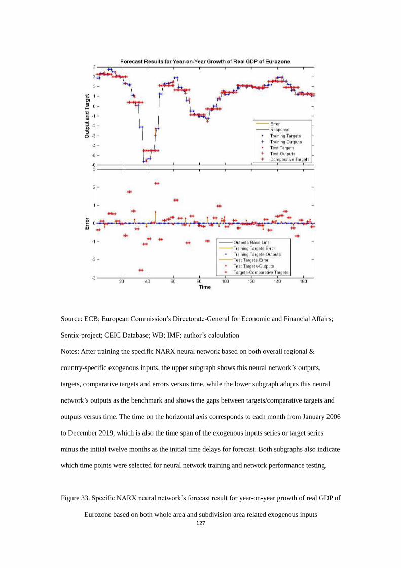
127

Source: ECB; European Commission’s Directorate-General for Economic and Financial Affairs;

Sentix-project; CEIC Database; WB; IMF; author’s calculation

Notes: After training the specific NARX neural network based on both overall regional &

country-specific exogenous inputs, the upper subgraph shows this neural network’s outputs,

targets, comparative targets and errors versus time, while the lower subgraph adopts this neural

network’s outputs as the benchmark and shows the gaps between targets/comparative targets and

outputs versus time. The time on the horizontal axis corresponds to each month from January 2006

to December 2019, which is also the time span of the exogenous inputs series or target series

minus the initial twelve months as the initial time delays for forecast. Both subgraphs also indicate

which time points were selected for neural network training and network performance testing.

Figure 33. Specific NARX neural network’s forecast result for year-on-year growth of real GDP of

Eurozone based on both whole area and subdivision area related exogenous inputs

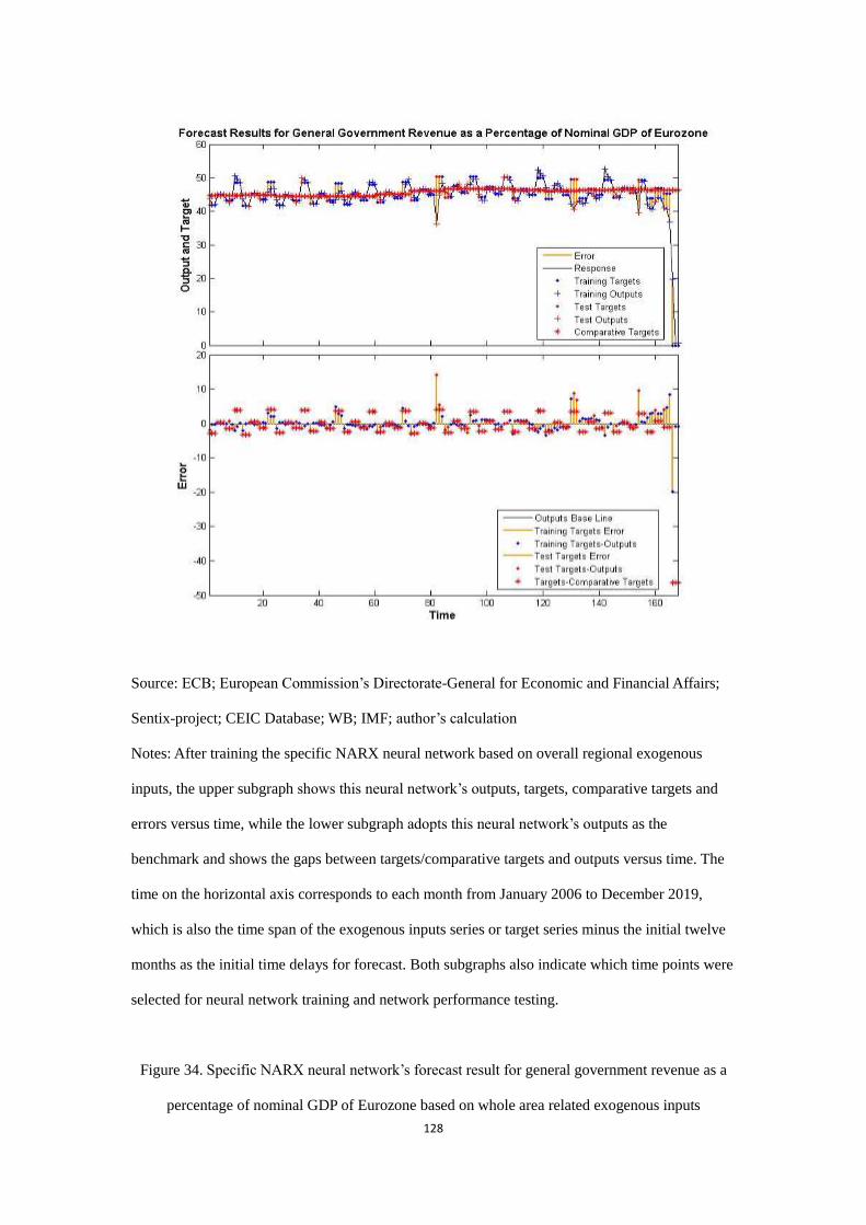
128

Source: ECB; European Commission’s Directorate-General for Economic and Financial Affairs;

Sentix-project; CEIC Database; WB; IMF; author’s calculation

Notes: After training the specific NARX neural network based on overall regional exogenous

inputs, the upper subgraph shows this neural network’s outputs, targets, comparative targets and

errors versus time, while the lower subgraph adopts this neural network’s outputs as the

benchmark and shows the gaps between targets/comparative targets and outputs versus time. The

time on the horizontal axis corresponds to each month from January 2006 to December 2019,

which is also the time span of the exogenous inputs series or target series minus the initial twelve

months as the initial time delays for forecast. Both subgraphs also indicate which time points were

selected for neural network training and network performance testing.

Figure 34. Specific NARX neural network’s forecast result for general government revenue as a

percentage of nominal GDP of Eurozone based on whole area related exogenous inputs

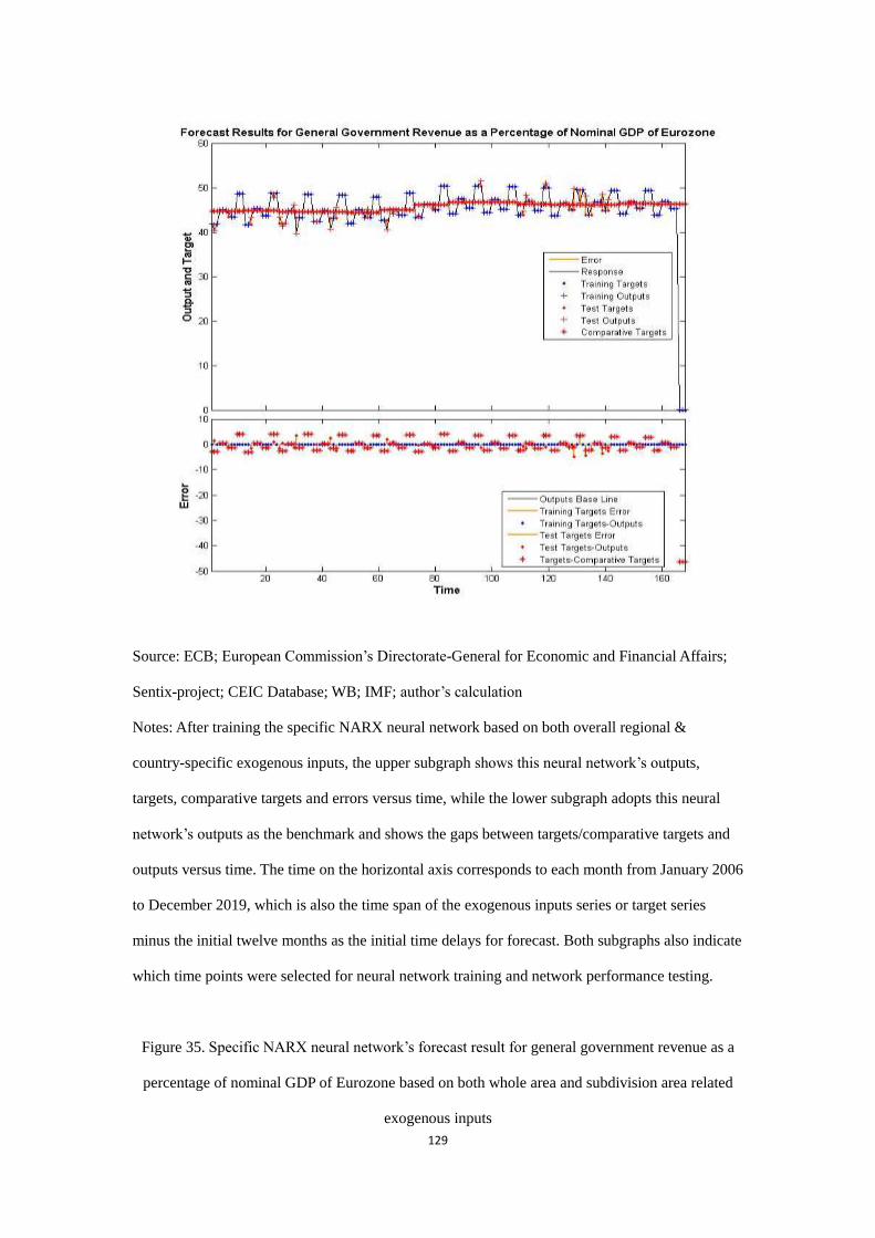
129

Source: ECB; European Commission’s Directorate-General for Economic and Financial Affairs;

Sentix-project; CEIC Database; WB; IMF; author’s calculation

Notes: After training the specific NARX neural network based on both overall regional &

country-specific exogenous inputs, the upper subgraph shows this neural network’s outputs,

targets, comparative targets and errors versus time, while the lower subgraph adopts this neural

network’s outputs as the benchmark and shows the gaps between targets/comparative targets and

outputs versus time. The time on the horizontal axis corresponds to each month from January 2006

to December 2019, which is also the time span of the exogenous inputs series or target series

minus the initial twelve months as the initial time delays for forecast. Both subgraphs also indicate

which time points were selected for neural network training and network performance testing.

Figure 35. Specific NARX neural network’s forecast result for general government revenue as a

percentage of nominal GDP of Eurozone based on both whole area and subdivision area related

exogenous inputs

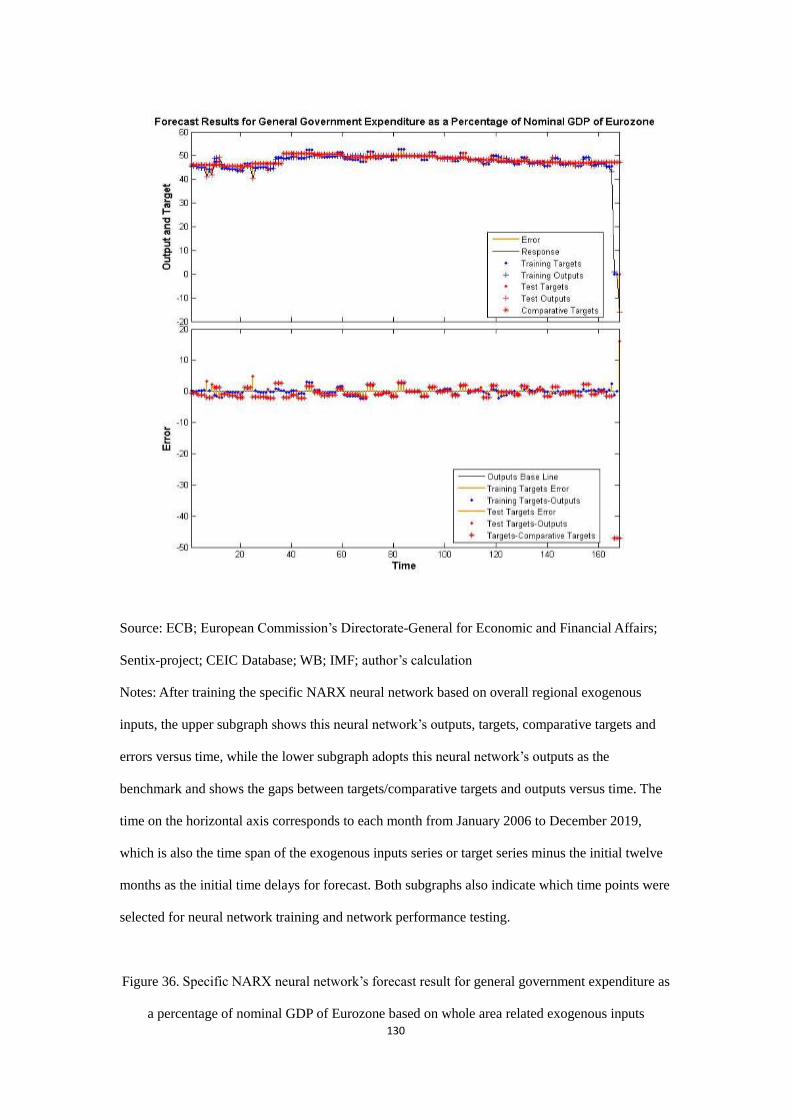
130

Source: ECB; European Commission’s Directorate-General for Economic and Financial Affairs;

Sentix-project; CEIC Database; WB; IMF; author’s calculation

Notes: After training the specific NARX neural network based on overall regional exogenous

inputs, the upper subgraph shows this neural network’s outputs, targets, comparative targets and

errors versus time, while the lower subgraph adopts this neural network’s outputs as the

benchmark and shows the gaps between targets/comparative targets and outputs versus time. The

time on the horizontal axis corresponds to each month from January 2006 to December 2019,

which is also the time span of the exogenous inputs series or target series minus the initial twelve

months as the initial time delays for forecast. Both subgraphs also indicate which time points were

selected for neural network training and network performance testing.

Figure 36. Specific NARX neural network’s forecast result for general government expenditure as

a percentage of nominal GDP of Eurozone based on whole area related exogenous inputs

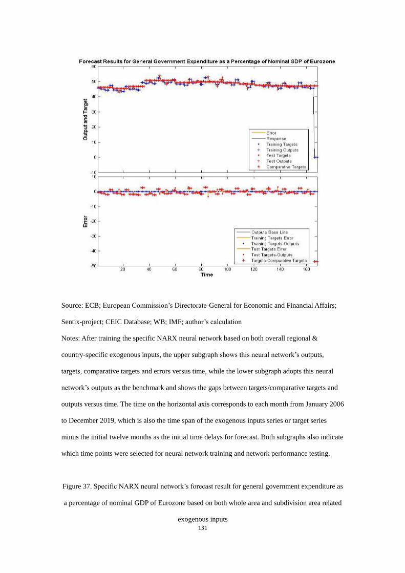
131

Source: ECB; European Commission’s Directorate-General for Economic and Financial Affairs;

Sentix-project; CEIC Database; WB; IMF; author’s calculation

Notes: After training the specific NARX neural network based on both overall regional &

country-specific exogenous inputs, the upper subgraph shows this neural network’s outputs,

targets, comparative targets and errors versus time, while the lower subgraph adopts this neural

network’s outputs as the benchmark and shows the gaps between targets/comparative targets and

outputs versus time. The time on the horizontal axis corresponds to each month from January 2006

to December 2019, which is also the time span of the exogenous inputs series or target series

minus the initial twelve months as the initial time delays for forecast. Both subgraphs also indicate

which time points were selected for neural network training and network performance testing.

Figure 37. Specific NARX neural network’s forecast result for general government expenditure as

a percentage of nominal GDP of Eurozone based on both whole area and subdivision area related

exogenous inputs

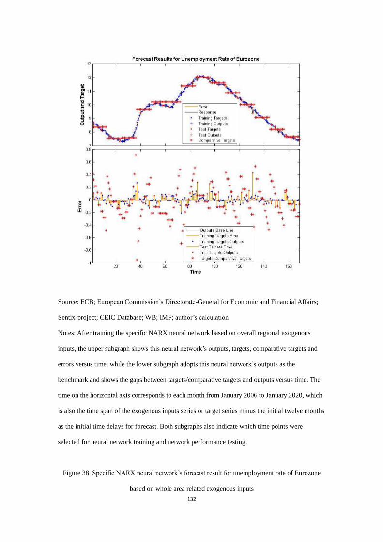
132

Source: ECB; European Commission’s Directorate-General for Economic and Financial Affairs;

Sentix-project; CEIC Database; WB; IMF; author’s calculation

Notes: After training the specific NARX neural network based on overall regional exogenous

inputs, the upper subgraph shows this neural network’s outputs, targets, comparative targets and

errors versus time, while the lower subgraph adopts this neural network’s outputs as the

benchmark and shows the gaps between targets/comparative targets and outputs versus time. The

time on the horizontal axis corresponds to each month from January 2006 to January 2020, which

is also the time span of the exogenous inputs series or target series minus the initial twelve months

as the initial time delays for forecast. Both subgraphs also indicate which time points were

selected for neural network training and network performance testing.

Figure 38. Specific NARX neural network’s forecast result for unemployment rate of Eurozone

based on whole area related exogenous inputs

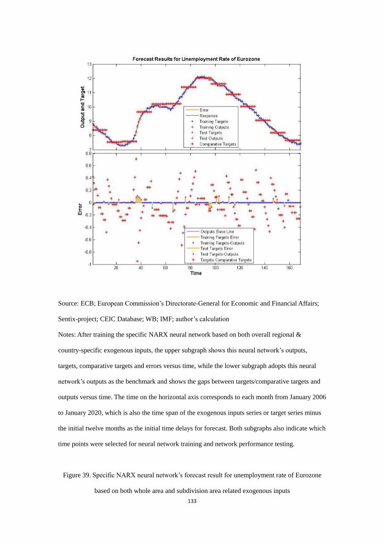
133

Source: ECB; European Commission’s Directorate-General for Economic and Financial Affairs;

Sentix-project; CEIC Database; WB; IMF; author’s calculation

Notes: After training the specific NARX neural network based on both overall regional &

country-specific exogenous inputs, the upper subgraph shows this neural network’s outputs,

targets, comparative targets and errors versus time, while the lower subgraph adopts this neural

network’s outputs as the benchmark and shows the gaps between targets/comparative targets and

outputs versus time. The time on the horizontal axis corresponds to each month from January 2006

to January 2020, which is also the time span of the exogenous inputs series or target series minus

the initial twelve months as the initial time delays for forecast. Both subgraphs also indicate which

time points were selected for neural network training and network performance testing.

Figure 39. Specific NARX neural network’s forecast result for unemployment rate of Eurozone

based on both whole area and subdivision area related exogenous inputs

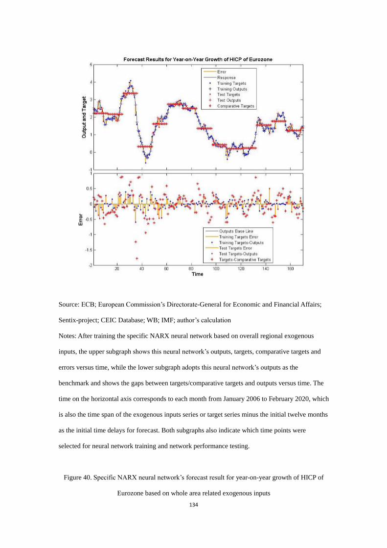
134

Source: ECB; European Commission’s Directorate-General for Economic and Financial Affairs;

Sentix-project; CEIC Database; WB; IMF; author’s calculation

Notes: After training the specific NARX neural network based on overall regional exogenous

inputs, the upper subgraph shows this neural network’s outputs, targets, comparative targets and

errors versus time, while the lower subgraph adopts this neural network’s outputs as the

benchmark and shows the gaps between targets/comparative targets and outputs versus time. The

time on the horizontal axis corresponds to each month from January 2006 to February 2020, which

is also the time span of the exogenous inputs series or target series minus the initial twelve months

as the initial time delays for forecast. Both subgraphs also indicate which time points were

selected for neural network training and network performance testing.

Figure 40. Specific NARX neural network’s forecast result for year-on-year growth of HICP of

Eurozone based on whole area related exogenous inputs

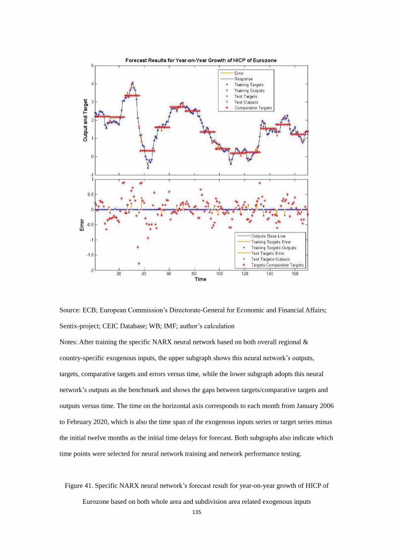
135

Source: ECB; European Commission’s Directorate-General for Economic and Financial Affairs;

Sentix-project; CEIC Database; WB; IMF; author’s calculation

Notes: After training the specific NARX neural network based on both overall regional &

country-specific exogenous inputs, the upper subgraph shows this neural network’s outputs,

targets, comparative targets and errors versus time, while the lower subgraph adopts this neural

network’s outputs as the benchmark and shows the gaps between targets/comparative targets and

outputs versus time. The time on the horizontal axis corresponds to each month from January 2006

to February 2020, which is also the time span of the exogenous inputs series or target series minus

the initial twelve months as the initial time delays for forecast. Both subgraphs also indicate which

time points were selected for neural network training and network performance testing.

Figure 41. Specific NARX neural network’s forecast result for year-on-year growth of HICP of

Eurozone based on both whole area and subdivision area related exogenous inputs

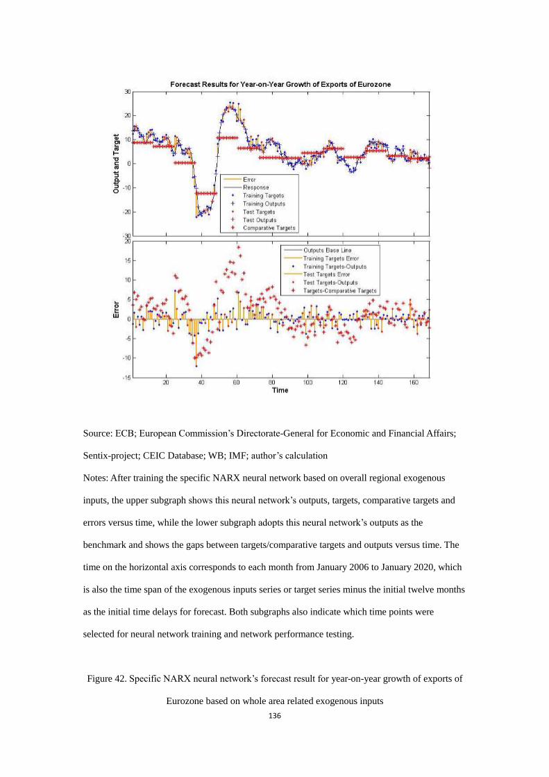
136

Source: ECB; European Commission’s Directorate-General for Economic and Financial Affairs;

Sentix-project; CEIC Database; WB; IMF; author’s calculation

Notes: After training the specific NARX neural network based on overall regional exogenous

inputs, the upper subgraph shows this neural network’s outputs, targets, comparative targets and

errors versus time, while the lower subgraph adopts this neural network’s outputs as the

benchmark and shows the gaps between targets/comparative targets and outputs versus time. The

time on the horizontal axis corresponds to each month from January 2006 to January 2020, which

is also the time span of the exogenous inputs series or target series minus the initial twelve months

as the initial time delays for forecast. Both subgraphs also indicate which time points were

selected for neural network training and network performance testing.

Figure 42. Specific NARX neural network’s forecast result for year-on-year growth of exports of

Eurozone based on whole area related exogenous inputs

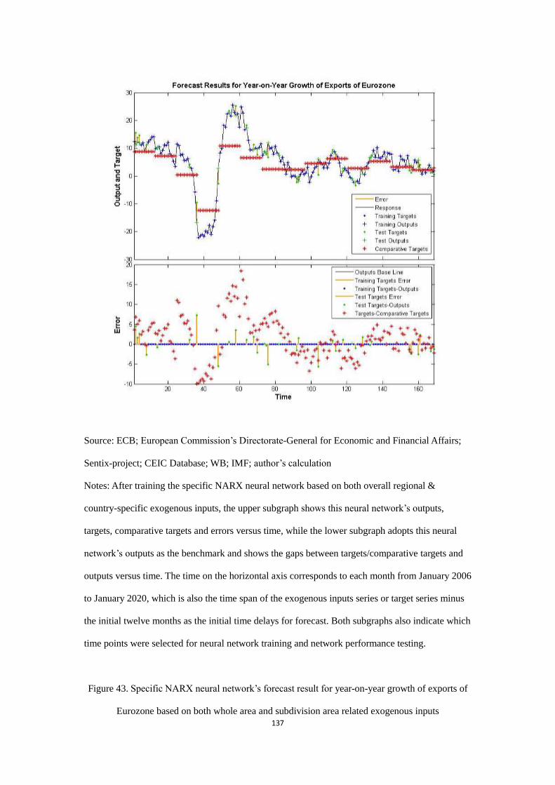
137

Source: ECB; European Commission’s Directorate-General for Economic and Financial Affairs;

Sentix-project; CEIC Database; WB; IMF; author’s calculation

Notes: After training the specific NARX neural network based on both overall regional &

country-specific exogenous inputs, the upper subgraph shows this neural network’s outputs,

targets, comparative targets and errors versus time, while the lower subgraph adopts this neural

network’s outputs as the benchmark and shows the gaps between targets/comparative targets and

outputs versus time. The time on the horizontal axis corresponds to each month from January 2006

to January 2020, which is also the time span of the exogenous inputs series or target series minus

the initial twelve months as the initial time delays for forecast. Both subgraphs also indicate which

time points were selected for neural network training and network performance testing.

Figure 43. Specific NARX neural network’s forecast result for year-on-year growth of exports of

Eurozone based on both whole area and subdivision area related exogenous inputs

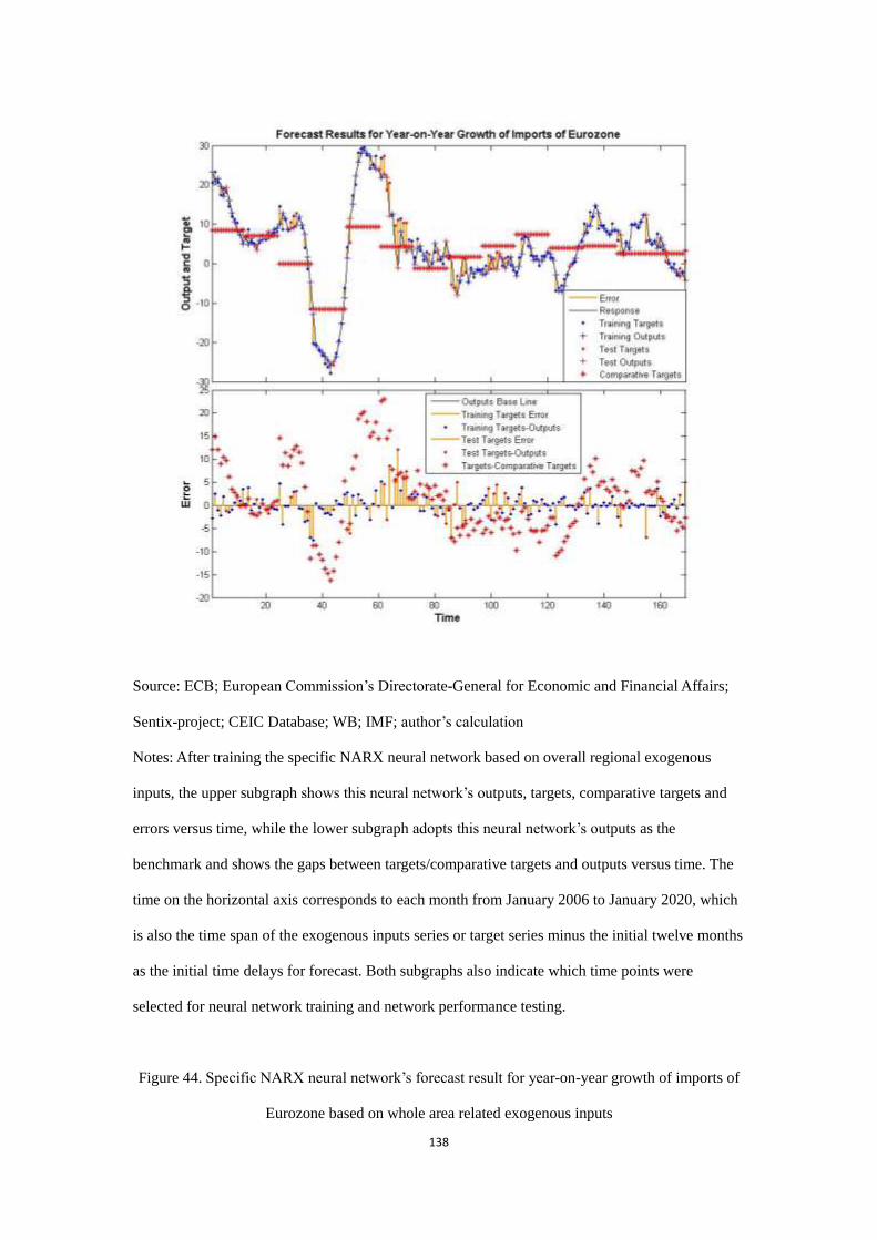
138

Source: ECB; European Commission’s Directorate-General for Economic and Financial Affairs;

Sentix-project; CEIC Database; WB; IMF; author’s calculation

Notes: After training the specific NARX neural network based on overall regional exogenous

inputs, the upper subgraph shows this neural network’s outputs, targets, comparative targets and

errors versus time, while the lower subgraph adopts this neural network’s outputs as the

benchmark and shows the gaps between targets/comparative targets and outputs versus time. The

time on the horizontal axis corresponds to each month from January 2006 to January 2020, which

is also the time span of the exogenous inputs series or target series minus the initial twelve months

as the initial time delays for forecast. Both subgraphs also indicate which time points were

selected for neural network training and network performance testing.

Figure 44. Specific NARX neural network’s forecast result for year-on-year growth of imports of

Eurozone based on whole area related exogenous inputs

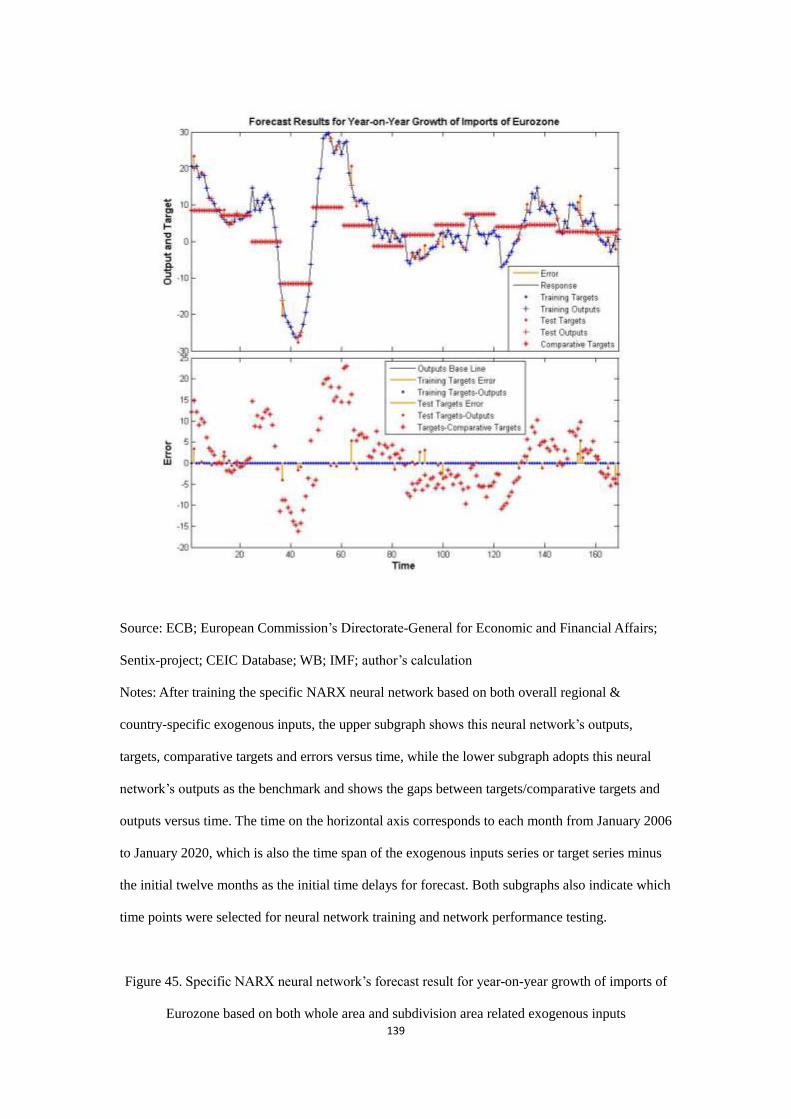
139

Source: ECB; European Commission’s Directorate-General for Economic and Financial Affairs;

Sentix-project; CEIC Database; WB; IMF; author’s calculation

Notes: After training the specific NARX neural network based on both overall regional &

country-specific exogenous inputs, the upper subgraph shows this neural network’s outputs,

targets, comparative targets and errors versus time, while the lower subgraph adopts this neural

network’s outputs as the benchmark and shows the gaps between targets/comparative targets and

outputs versus time. The time on the horizontal axis corresponds to each month from January 2006

to January 2020, which is also the time span of the exogenous inputs series or target series minus

the initial twelve months as the initial time delays for forecast. Both subgraphs also indicate which

time points were selected for neural network training and network performance testing.

Figure 45. Specific NARX neural network’s forecast result for year-on-year growth of imports of

Eurozone based on both whole area and subdivision area related exogenous inputs

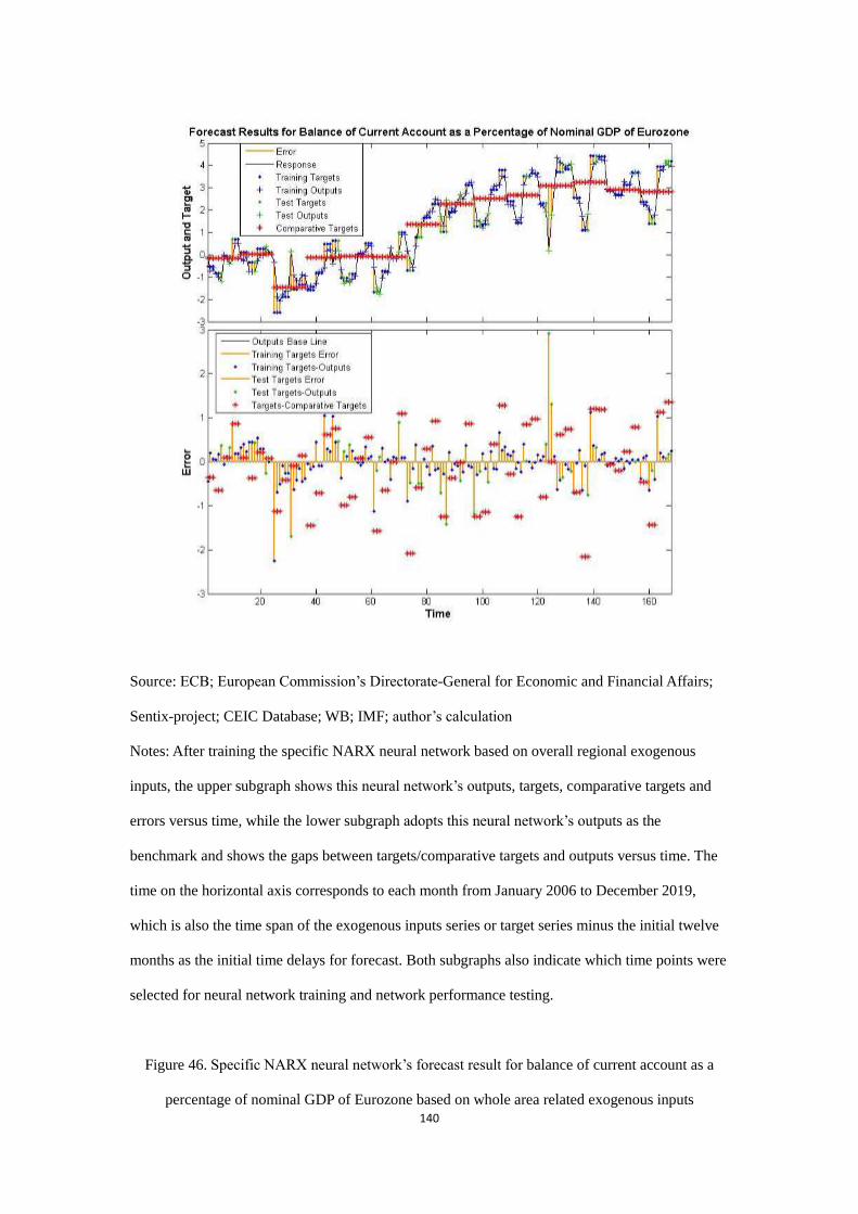
140

Source: ECB; European Commission’s Directorate-General for Economic and Financial Affairs;

Sentix-project; CEIC Database; WB; IMF; author’s calculation

Notes: After training the specific NARX neural network based on overall regional exogenous

inputs, the upper subgraph shows this neural network’s outputs, targets, comparative targets and

errors versus time, while the lower subgraph adopts this neural network’s outputs as the

benchmark and shows the gaps between targets/comparative targets and outputs versus time. The

time on the horizontal axis corresponds to each month from January 2006 to December 2019,

which is also the time span of the exogenous inputs series or target series minus the initial twelve

months as the initial time delays for forecast. Both subgraphs also indicate which time points were

selected for neural network training and network performance testing.

Figure 46. Specific NARX neural network’s forecast result for balance of current account as a

percentage of nominal GDP of Eurozone based on whole area related exogenous inputs

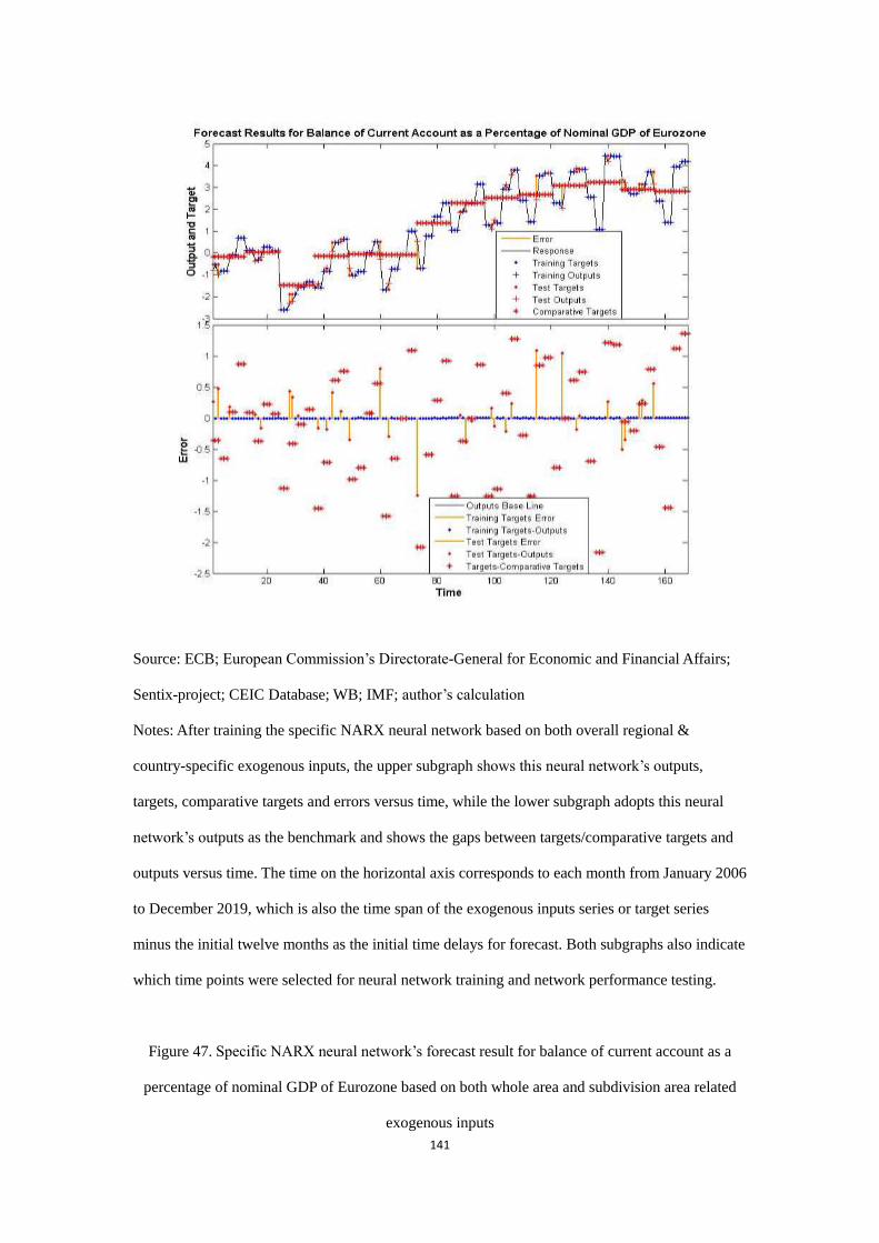
141

Source: ECB; European Commission’s Directorate-General for Economic and Financial Affairs;

Sentix-project; CEIC Database; WB; IMF; author’s calculation

Notes: After training the specific NARX neural network based on both overall regional &

country-specific exogenous inputs, the upper subgraph shows this neural network’s outputs,

targets, comparative targets and errors versus time, while the lower subgraph adopts this neural

network’s outputs as the benchmark and shows the gaps between targets/comparative targets and

outputs versus time. The time on the horizontal axis corresponds to each month from January 2006

to December 2019, which is also the time span of the exogenous inputs series or target series

minus the initial twelve months as the initial time delays for forecast. Both subgraphs also indicate

which time points were selected for neural network training and network performance testing.

Figure 47. Specific NARX neural network’s forecast result for balance of current account as a

percentage of nominal GDP of Eurozone based on both whole area and subdivision area related

exogenous inputs

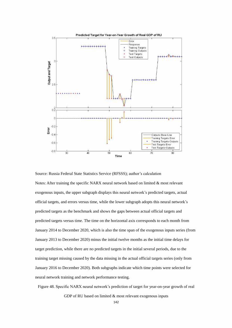
142

Source: Russia Federal State Statistics Service (RFSSS); author’s calculation

Notes: After training the specific NARX neural network based on limited & most relevant

exogenous inputs, the upper subgraph displays this neural network’s predicted targets, actual

official targets, and errors versus time, while the lower subgraph adopts this neural network’s

predicted targets as the benchmark and shows the gaps between actual official targets and

predicted targets versus time. The time on the horizontal axis corresponds to each month from

January 2014 to December 2020, which is also the time span of the exogenous inputs series (from

January 2013 to December 2020) minus the initial twelve months as the initial time delays for

target prediction, while there are no predicted targets in the initial several periods, due to the

training target missing caused by the data missing in the actual official targets series (only from

January 2016 to December 2020). Both subgraphs indicate which time points were selected for

neural network training and network performance testing.

Figure 48. Specific NARX neural network’s prediction of target for year-on-year growth of real

GDP of RU based on limited & most relevant exogenous inputs

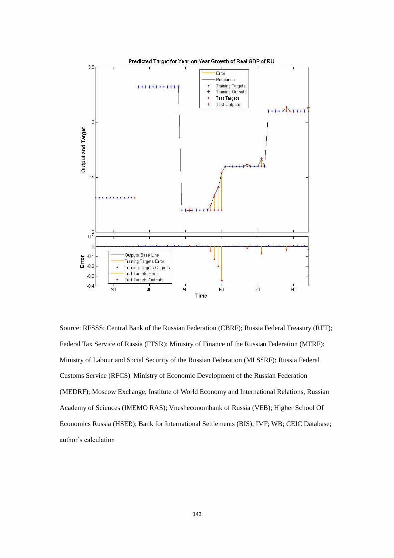
143

Source: RFSSS; Central Bank of the Russian Federation (CBRF); Russia Federal Treasury (RFT);

Federal Tax Service of Russia (FTSR); Ministry of Finance of the Russian Federation (MFRF);

Ministry of Labour and Social Security of the Russian Federation (MLSSRF); Russia Federal

Customs Service (RFCS); Ministry of Economic Development of the Russian Federation

(MEDRF); Moscow Exchange; Institute of World Economy and International Relations, Russian

Academy of Sciences (IMEMO RAS); Vnesheconombank of Russia (VEB); Higher School Of

Economics Russia (HSER); Bank for International Settlements (BIS); IMF; WB; CEIC Database;

author’s calculation

144

Notes: After training the specific NARX neural network based on abundant & comprehensive

exogenous inputs, the upper subgraph displays this neural network’s predicted targets, actual

official targets, and errors versus time, while the lower subgraph adopts this neural network’s

predicted targets as the benchmark and shows the gaps between actual official targets and

predicted targets versus time. The time on the horizontal axis corresponds to each month from

January 2014 to December 2020, which is also the time span of the exogenous inputs series (from

January 2013 to December 2020) minus the initial twelve months as the initial time delays for

target prediction, while there are no predicted targets in the initial several periods, due to the

training target missing caused by the data missing in the actual official targets series (only from

January 2016 to December 2020). Both subgraphs indicate which time points were selected for

neural network training and network performance testing.

Figure 49. Specific NARX neural network’s prediction of target for year-on-year growth of real

GDP of RU based on abundant & comprehensive exogenous inputs

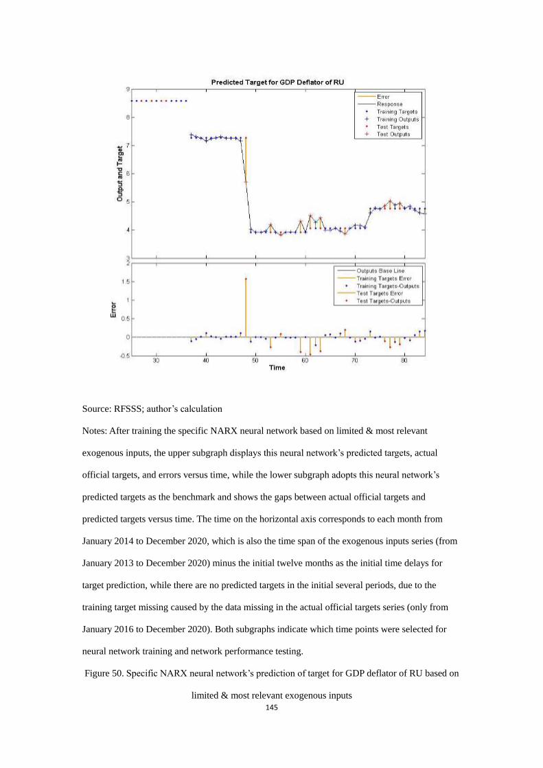
145

Source: RFSSS; author’s calculation

Notes: After training the specific NARX neural network based on limited & most relevant

exogenous inputs, the upper subgraph displays this neural network’s predicted targets, actual

official targets, and errors versus time, while the lower subgraph adopts this neural network’s

predicted targets as the benchmark and shows the gaps between actual official targets and

predicted targets versus time. The time on the horizontal axis corresponds to each month from

January 2014 to December 2020, which is also the time span of the exogenous inputs series (from

January 2013 to December 2020) minus the initial twelve months as the initial time delays for

target prediction, while there are no predicted targets in the initial several periods, due to the

training target missing caused by the data missing in the actual official targets series (only from

January 2016 to December 2020). Both subgraphs indicate which time points were selected for

neural network training and network performance testing.

Figure 50. Specific NARX neural network’s prediction of target for GDP deflator of RU based on

limited & most relevant exogenous inputs

146

Source: RFSSS; CBRF; RFT; FTSR; MFRF; MLSSRF; RFCS; MEDRF; Moscow Exchange;

IMEMO RAS; VEB; HSER; BIS; IMF; WB; CEIC Database; author’s calculation

Notes: After training the specific NARX neural network based on abundant & comprehensive

exogenous inputs, the upper subgraph displays this neural network’s predicted targets, actual

official targets, and errors versus time, while the lower subgraph adopts this neural network’s

predicted targets as the benchmark and shows the gaps between actual official targets and

predicted targets versus time. The time on the horizontal axis corresponds to each month from

January 2014 to December 2020, which is also the time span of the exogenous inputs series (from

January 2013 to December 2020) minus the initial twelve months as the initial time delays for

target prediction, while there are no predicted targets in the initial several periods, due to the

training target missing caused by the data missing in the actual official targets series (only from

January 2016 to December 2020). Both subgraphs indicate which time points were selected for

neural network training and network performance testing.

Figure 51. Specific NARX neural network’s prediction of target for GDP deflator of RU based on

abundant & comprehensive exogenous inputs

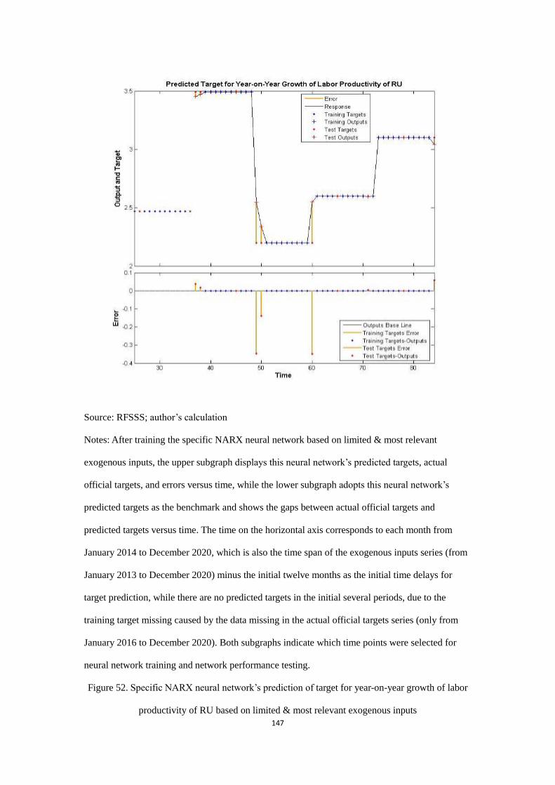
147

Source: RFSSS; author’s calculation

Notes: After training the specific NARX neural network based on limited & most relevant

exogenous inputs, the upper subgraph displays this neural network’s predicted targets, actual

official targets, and errors versus time, while the lower subgraph adopts this neural network’s

predicted targets as the benchmark and shows the gaps between actual official targets and

predicted targets versus time. The time on the horizontal axis corresponds to each month from

January 2014 to December 2020, which is also the time span of the exogenous inputs series (from

January 2013 to December 2020) minus the initial twelve months as the initial time delays for

target prediction, while there are no predicted targets in the initial several periods, due to the

training target missing caused by the data missing in the actual official targets series (only from

January 2016 to December 2020). Both subgraphs indicate which time points were selected for

neural network training and network performance testing.

Figure 52. Specific NARX neural network’s prediction of target for year-on-year growth of labor

productivity of RU based on limited & most relevant exogenous inputs

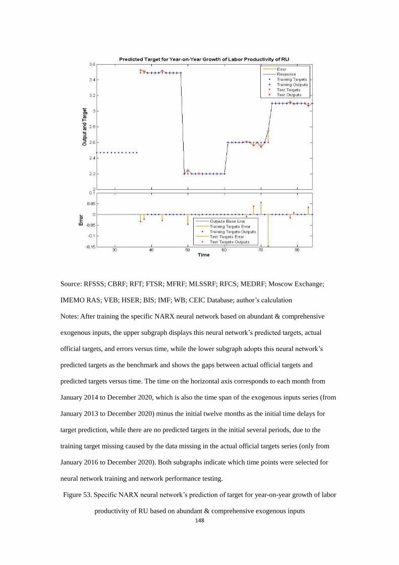
148

Source: RFSSS; CBRF; RFT; FTSR; MFRF; MLSSRF; RFCS; MEDRF; Moscow Exchange;

IMEMO RAS; VEB; HSER; BIS; IMF; WB; CEIC Database; author’s calculation

Notes: After training the specific NARX neural network based on abundant & comprehensive

exogenous inputs, the upper subgraph displays this neural network’s predicted targets, actual

official targets, and errors versus time, while the lower subgraph adopts this neural network’s

predicted targets as the benchmark and shows the gaps between actual official targets and

predicted targets versus time. The time on the horizontal axis corresponds to each month from

January 2014 to December 2020, which is also the time span of the exogenous inputs series (from

January 2013 to December 2020) minus the initial twelve months as the initial time delays for

target prediction, while there are no predicted targets in the initial several periods, due to the

training target missing caused by the data missing in the actual official targets series (only from

January 2016 to December 2020). Both subgraphs indicate which time points were selected for

neural network training and network performance testing.

Figure 53. Specific NARX neural network’s prediction of target for year-on-year growth of labor

productivity of RU based on abundant & comprehensive exogenous inputs

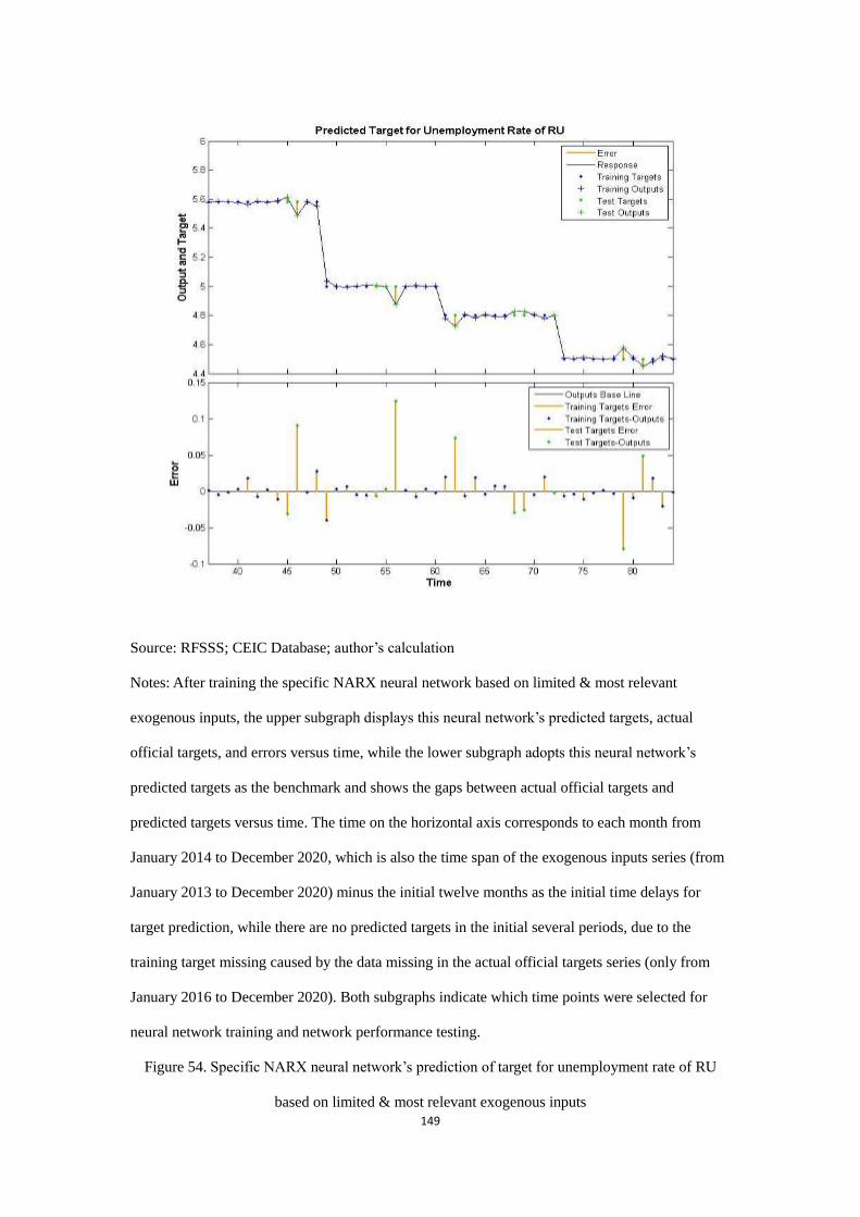
149

Source: RFSSS; CEIC Database; author’s calculation

Notes: After training the specific NARX neural network based on limited & most relevant

exogenous inputs, the upper subgraph displays this neural network’s predicted targets, actual

official targets, and errors versus time, while the lower subgraph adopts this neural network’s

predicted targets as the benchmark and shows the gaps between actual official targets and

predicted targets versus time. The time on the horizontal axis corresponds to each month from

January 2014 to December 2020, which is also the time span of the exogenous inputs series (from

January 2013 to December 2020) minus the initial twelve months as the initial time delays for

target prediction, while there are no predicted targets in the initial several periods, due to the

training target missing caused by the data missing in the actual official targets series (only from

January 2016 to December 2020). Both subgraphs indicate which time points were selected for

neural network training and network performance testing.

Figure 54. Specific NARX neural network’s prediction of target for unemployment rate of RU

based on limited & most relevant exogenous inputs

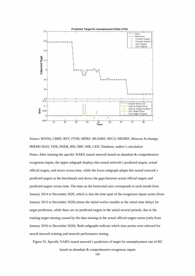
150

Source: RFSSS; CBRF; RFT; FTSR; MFRF; MLSSRF; RFCS; MEDRF; Moscow Exchange;

IMEMO RAS; VEB; HSER; BIS; IMF; WB; CEIC Database; author’s calculation

Notes: After training the specific NARX neural network based on abundant & comprehensive

exogenous inputs, the upper subgraph displays this neural network’s predicted targets, actual

official targets, and errors versus time, while the lower subgraph adopts this neural network’s

predicted targets as the benchmark and shows the gaps between actual official targets and

predicted targets versus time. The time on the horizontal axis corresponds to each month from

January 2014 to December 2020, which is also the time span of the exogenous inputs series (from

January 2013 to December 2020) minus the initial twelve months as the initial time delays for

target prediction, while there are no predicted targets in the initial several periods, due to the

training target missing caused by the data missing in the actual official targets series (only from

January 2016 to December 2020). Both subgraphs indicate which time points were selected for

neural network training and network performance testing.

Figure 55. Specific NARX neural network’s prediction of target for unemployment rate of RU

based on abundant & comprehensive exogenous inputs

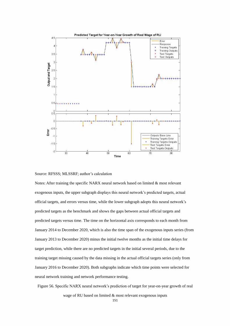
151

Source: RFSSS; MLSSRF; author’s calculation

Notes: After training the specific NARX neural network based on limited & most relevant

exogenous inputs, the upper subgraph displays this neural network’s predicted targets, actual

official targets, and errors versus time, while the lower subgraph adopts this neural network’s

predicted targets as the benchmark and shows the gaps between actual official targets and

predicted targets versus time. The time on the horizontal axis corresponds to each month from

January 2014 to December 2020, which is also the time span of the exogenous inputs series (from

January 2013 to December 2020) minus the initial twelve months as the initial time delays for

target prediction, while there are no predicted targets in the initial several periods, due to the

training target missing caused by the data missing in the actual official targets series (only from

January 2016 to December 2020). Both subgraphs indicate which time points were selected for

neural network training and network performance testing.

Figure 56. Specific NARX neural network’s prediction of target for year-on-year growth of real

wage of RU based on limited & most relevant exogenous inputs

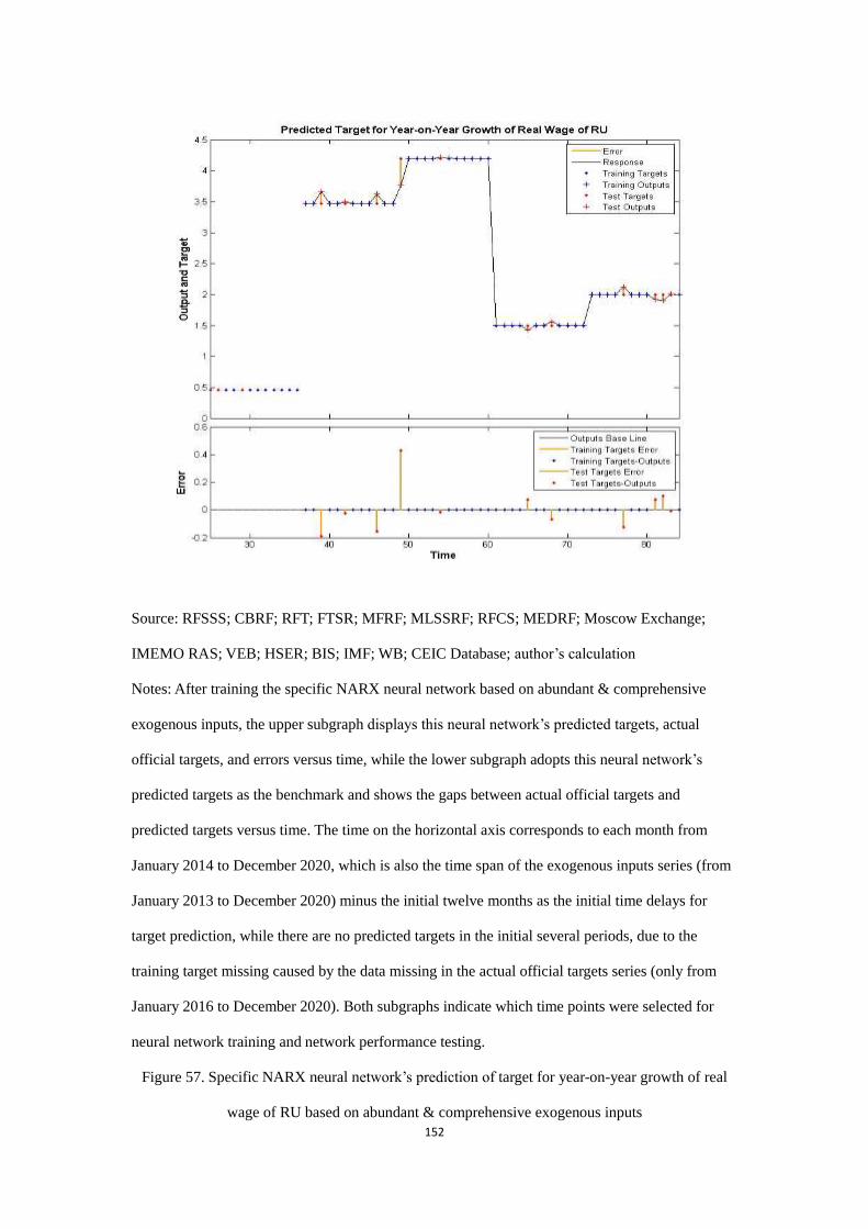
152

Source: RFSSS; CBRF; RFT; FTSR; MFRF; MLSSRF; RFCS; MEDRF; Moscow Exchange;

IMEMO RAS; VEB; HSER; BIS; IMF; WB; CEIC Database; author’s calculation

Notes: After training the specific NARX neural network based on abundant & comprehensive

exogenous inputs, the upper subgraph displays this neural network’s predicted targets, actual

official targets, and errors versus time, while the lower subgraph adopts this neural network’s

predicted targets as the benchmark and shows the gaps between actual official targets and

predicted targets versus time. The time on the horizontal axis corresponds to each month from

January 2014 to December 2020, which is also the time span of the exogenous inputs series (from

January 2013 to December 2020) minus the initial twelve months as the initial time delays for

target prediction, while there are no predicted targets in the initial several periods, due to the

training target missing caused by the data missing in the actual official targets series (only from

January 2016 to December 2020). Both subgraphs indicate which time points were selected for

neural network training and network performance testing.

Figure 57. Specific NARX neural network’s prediction of target for year-on-year growth of real

wage of RU based on abundant & comprehensive exogenous inputs

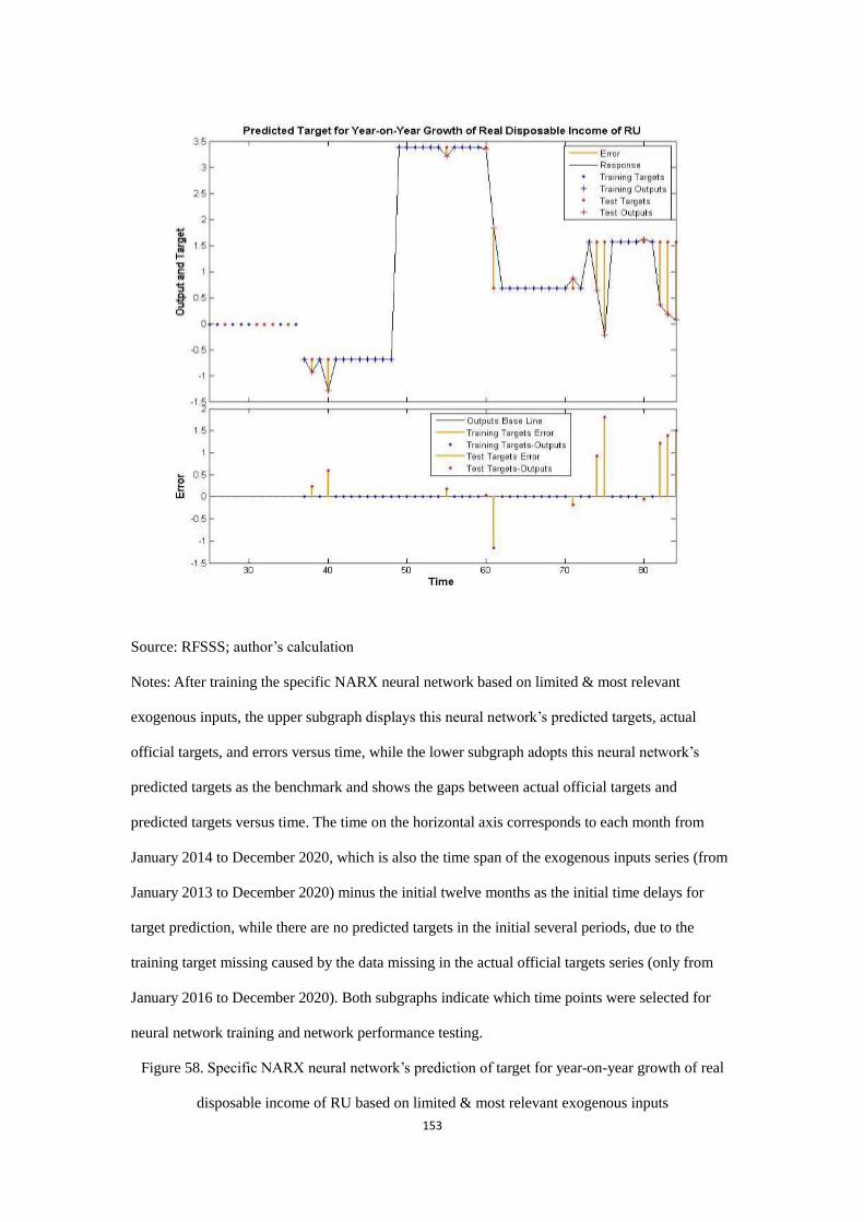
153

Source: RFSSS; author’s calculation

Notes: After training the specific NARX neural network based on limited & most relevant

exogenous inputs, the upper subgraph displays this neural network’s predicted targets, actual

official targets, and errors versus time, while the lower subgraph adopts this neural network’s

predicted targets as the benchmark and shows the gaps between actual official targets and

predicted targets versus time. The time on the horizontal axis corresponds to each month from

January 2014 to December 2020, which is also the time span of the exogenous inputs series (from

January 2013 to December 2020) minus the initial twelve months as the initial time delays for

target prediction, while there are no predicted targets in the initial several periods, due to the

training target missing caused by the data missing in the actual official targets series (only from

January 2016 to December 2020). Both subgraphs indicate which time points were selected for

neural network training and network performance testing.

Figure 58. Specific NARX neural network’s prediction of target for year-on-year growth of real

disposable income of RU based on limited & most relevant exogenous inputs

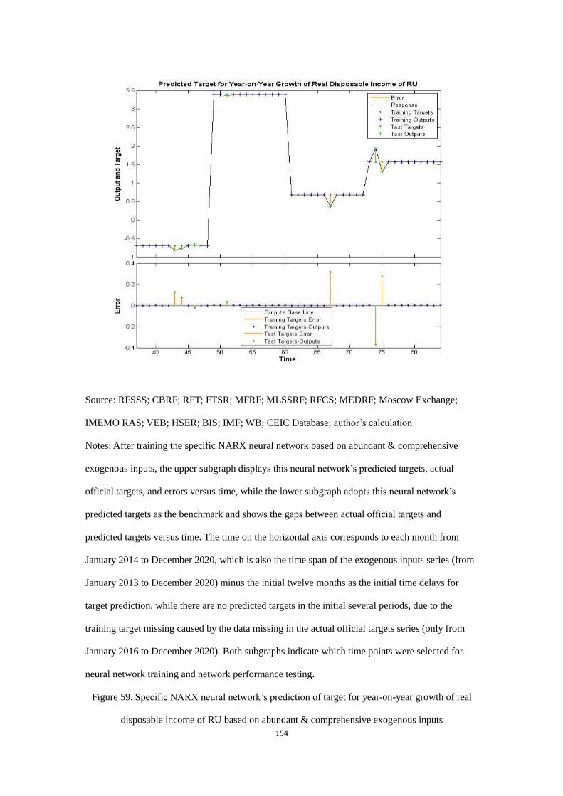
154

Source: RFSSS; CBRF; RFT; FTSR; MFRF; MLSSRF; RFCS; MEDRF; Moscow Exchange;

IMEMO RAS; VEB; HSER; BIS; IMF; WB; CEIC Database; author’s calculation

Notes: After training the specific NARX neural network based on abundant & comprehensive

exogenous inputs, the upper subgraph displays this neural network’s predicted targets, actual

official targets, and errors versus time, while the lower subgraph adopts this neural network’s

predicted targets as the benchmark and shows the gaps between actual official targets and

predicted targets versus time. The time on the horizontal axis corresponds to each month from

January 2014 to December 2020, which is also the time span of the exogenous inputs series (from

January 2013 to December 2020) minus the initial twelve months as the initial time delays for

target prediction, while there are no predicted targets in the initial several periods, due to the

training target missing caused by the data missing in the actual official targets series (only from

January 2016 to December 2020). Both subgraphs indicate which time points were selected for

neural network training and network performance testing.

Figure 59. Specific NARX neural network’s prediction of target for year-on-year growth of real

disposable income of RU based on abundant & comprehensive exogenous inputs

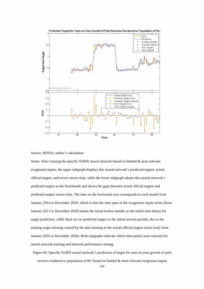
155

Source: RFSSS; author’s calculation

Notes: After training the specific NARX neural network based on limited & most relevant

exogenous inputs, the upper subgraph displays this neural network’s predicted targets, actual

official targets, and errors versus time, while the lower subgraph adopts this neural network’s

predicted targets as the benchmark and shows the gaps between actual official targets and

predicted targets versus time. The time on the horizontal axis corresponds to each month from

January 2014 to December 2020, which is also the time span of the exogenous inputs series (from

January 2013 to December 2020) minus the initial twelve months as the initial time delays for

target prediction, while there are no predicted targets in the initial several periods, due to the

training target missing caused by the data missing in the actual official targets series (only from

January 2016 to December 2020). Both subgraphs indicate which time points were selected for

neural network training and network performance testing.

Figure 60. Specific NARX neural network’s prediction of target for year-on-year growth of paid

services rendered to population of RU based on limited & most relevant exogenous inputs

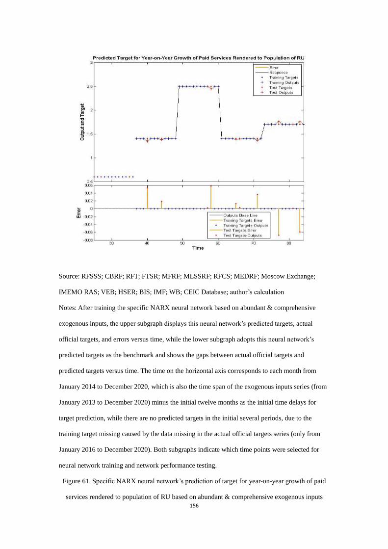
156

Source: RFSSS; CBRF; RFT; FTSR; MFRF; MLSSRF; RFCS; MEDRF; Moscow Exchange;

IMEMO RAS; VEB; HSER; BIS; IMF; WB; CEIC Database; author’s calculation

Notes: After training the specific NARX neural network based on abundant & comprehensive

exogenous inputs, the upper subgraph displays this neural network’s predicted targets, actual

official targets, and errors versus time, while the lower subgraph adopts this neural network’s

predicted targets as the benchmark and shows the gaps between actual official targets and

predicted targets versus time. The time on the horizontal axis corresponds to each month from

January 2014 to December 2020, which is also the time span of the exogenous inputs series (from

January 2013 to December 2020) minus the initial twelve months as the initial time delays for

target prediction, while there are no predicted targets in the initial several periods, due to the

training target missing caused by the data missing in the actual official targets series (only from

January 2016 to December 2020). Both subgraphs indicate which time points were selected for

neural network training and network performance testing.

Figure 61. Specific NARX neural network’s prediction of target for year-on-year growth of paid

services rendered to population of RU based on abundant & comprehensive exogenous inputs

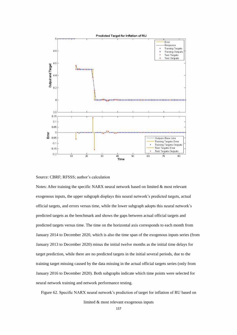
157

Source: CBRF; RFSSS; author’s calculation

Notes: After training the specific NARX neural network based on limited & most relevant

exogenous inputs, the upper subgraph displays this neural network’s predicted targets, actual

official targets, and errors versus time, while the lower subgraph adopts this neural network’s

predicted targets as the benchmark and shows the gaps between actual official targets and

predicted targets versus time. The time on the horizontal axis corresponds to each month from

January 2014 to December 2020, which is also the time span of the exogenous inputs series (from

January 2013 to December 2020) minus the initial twelve months as the initial time delays for

target prediction, while there are no predicted targets in the initial several periods, due to the

training target missing caused by the data missing in the actual official targets series (only from

January 2016 to December 2020). Both subgraphs indicate which time points were selected for

neural network training and network performance testing.

Figure 62. Specific NARX neural network’s prediction of target for inflation of RU based on

limited & most relevant exogenous inputs

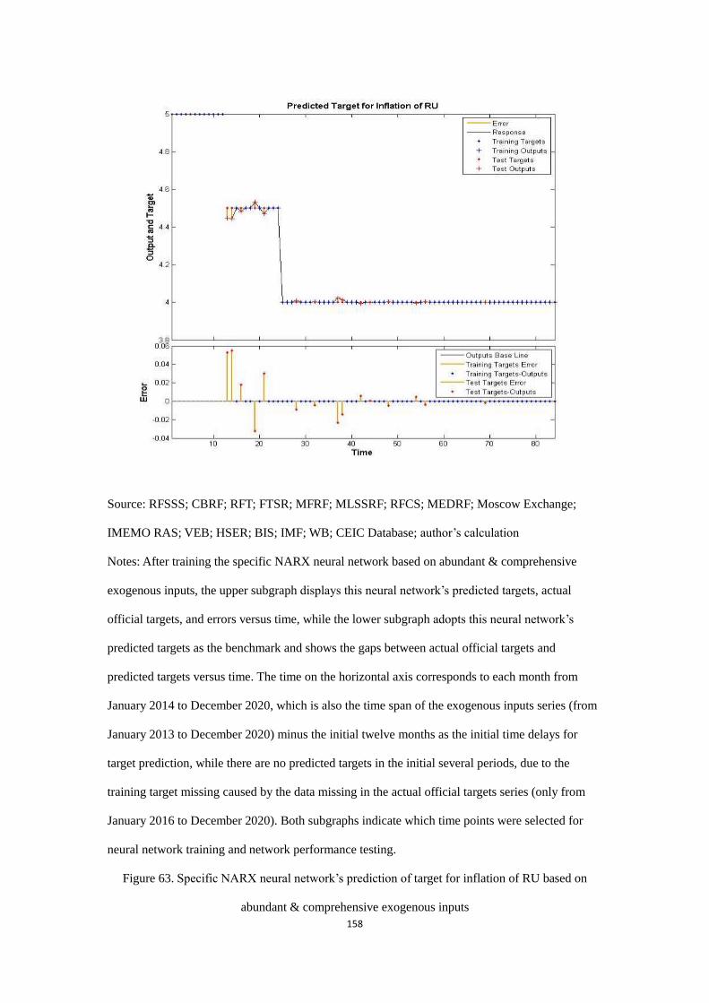
158

Source: RFSSS; CBRF; RFT; FTSR; MFRF; MLSSRF; RFCS; MEDRF; Moscow Exchange;

IMEMO RAS; VEB; HSER; BIS; IMF; WB; CEIC Database; author’s calculation

Notes: After training the specific NARX neural network based on abundant & comprehensive

exogenous inputs, the upper subgraph displays this neural network’s predicted targets, actual

official targets, and errors versus time, while the lower subgraph adopts this neural network’s

predicted targets as the benchmark and shows the gaps between actual official targets and

predicted targets versus time. The time on the horizontal axis corresponds to each month from

January 2014 to December 2020, which is also the time span of the exogenous inputs series (from

January 2013 to December 2020) minus the initial twelve months as the initial time delays for

target prediction, while there are no predicted targets in the initial several periods, due to the

training target missing caused by the data missing in the actual official targets series (only from

January 2016 to December 2020). Both subgraphs indicate which time points were selected for

neural network training and network performance testing.

Figure 63. Specific NARX neural network’s prediction of target for inflation of RU based on

abundant & comprehensive exogenous inputs

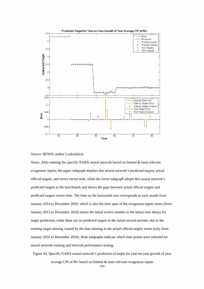
159

Source: RFSSS; author’s calculation

Notes: After training the specific NARX neural network based on limited & most relevant

exogenous inputs, the upper subgraph displays this neural network’s predicted targets, actual

official targets, and errors versus time, while the lower subgraph adopts this neural network’s

predicted targets as the benchmark and shows the gaps between actual official targets and

predicted targets versus time. The time on the horizontal axis corresponds to each month from

January 2014 to December 2020, which is also the time span of the exogenous inputs series (from

January 2013 to December 2020) minus the initial twelve months as the initial time delays for

target prediction, while there are no predicted targets in the initial several periods, due to the

training target missing caused by the data missing in the actual official targets series (only from

January 2016 to December 2020). Both subgraphs indicate which time points were selected for

neural network training and network performance testing.

Figure 64. Specific NARX neural network’s prediction of target for year-on-year growth of year

average CPI of RU based on limited & most relevant exogenous inputs

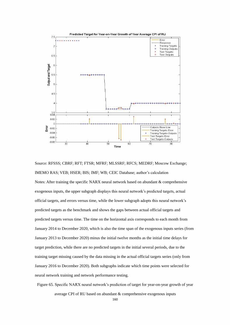
160

Source: RFSSS; CBRF; RFT; FTSR; MFRF; MLSSRF; RFCS; MEDRF; Moscow Exchange;

IMEMO RAS; VEB; HSER; BIS; IMF; WB; CEIC Database; author’s calculation

Notes: After training the specific NARX neural network based on abundant & comprehensive

exogenous inputs, the upper subgraph displays this neural network’s predicted targets, actual

official targets, and errors versus time, while the lower subgraph adopts this neural network’s

predicted targets as the benchmark and shows the gaps between actual official targets and

predicted targets versus time. The time on the horizontal axis corresponds to each month from

January 2014 to December 2020, which is also the time span of the exogenous inputs series (from

January 2013 to December 2020) minus the initial twelve months as the initial time delays for

target prediction, while there are no predicted targets in the initial several periods, due to the

training target missing caused by the data missing in the actual official targets series (only from

January 2016 to December 2020). Both subgraphs indicate which time points were selected for

neural network training and network performance testing.

Figure 65. Specific NARX neural network’s prediction of target for year-on-year growth of year

average CPI of RU based on abundant & comprehensive exogenous inputs

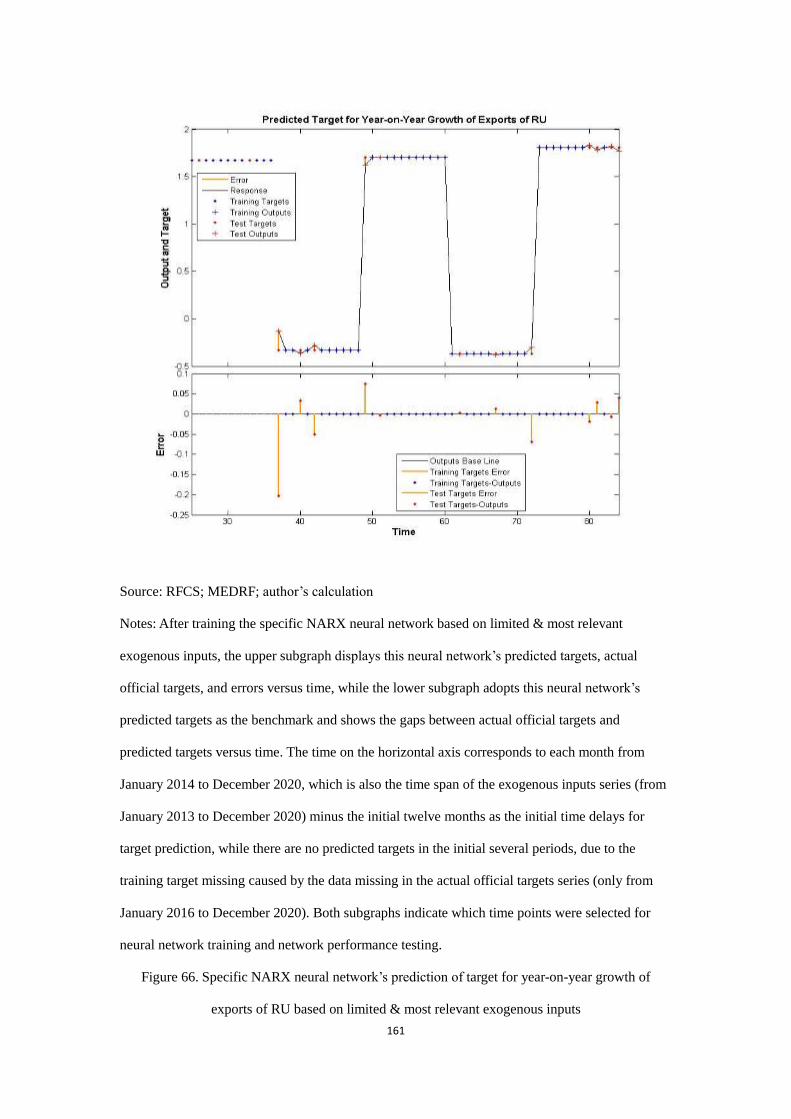
161

Source: RFCS; MEDRF; author’s calculation

Notes: After training the specific NARX neural network based on limited & most relevant

exogenous inputs, the upper subgraph displays this neural network’s predicted targets, actual

official targets, and errors versus time, while the lower subgraph adopts this neural network’s

predicted targets as the benchmark and shows the gaps between actual official targets and

predicted targets versus time. The time on the horizontal axis corresponds to each month from

January 2014 to December 2020, which is also the time span of the exogenous inputs series (from

January 2013 to December 2020) minus the initial twelve months as the initial time delays for

target prediction, while there are no predicted targets in the initial several periods, due to the

training target missing caused by the data missing in the actual official targets series (only from

January 2016 to December 2020). Both subgraphs indicate which time points were selected for

neural network training and network performance testing.

Figure 66. Specific NARX neural network’s prediction of target for year-on-year growth of

exports of RU based on limited & most relevant exogenous inputs

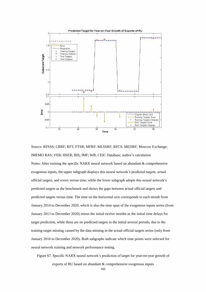
162

Source: RFSSS; CBRF; RFT; FTSR; MFRF; MLSSRF; RFCS; MEDRF; Moscow Exchange;

IMEMO RAS; VEB; HSER; BIS; IMF; WB; CEIC Database; author’s calculation

Notes: After training the specific NARX neural network based on abundant & comprehensive

exogenous inputs, the upper subgraph displays this neural network’s predicted targets, actual

official targets, and errors versus time, while the lower subgraph adopts this neural network’s

predicted targets as the benchmark and shows the gaps between actual official targets and

predicted targets versus time. The time on the horizontal axis corresponds to each month from

January 2014 to December 2020, which is also the time span of the exogenous inputs series (from

January 2013 to December 2020) minus the initial twelve months as the initial time delays for

target prediction, while there are no predicted targets in the initial several periods, due to the

training target missing caused by the data missing in the actual official targets series (only from

January 2016 to December 2020). Both subgraphs indicate which time points were selected for

neural network training and network performance testing.

Figure 67. Specific NARX neural network’s prediction of target for year-on-year growth of

exports of RU based on abundant & comprehensive exogenous inputs

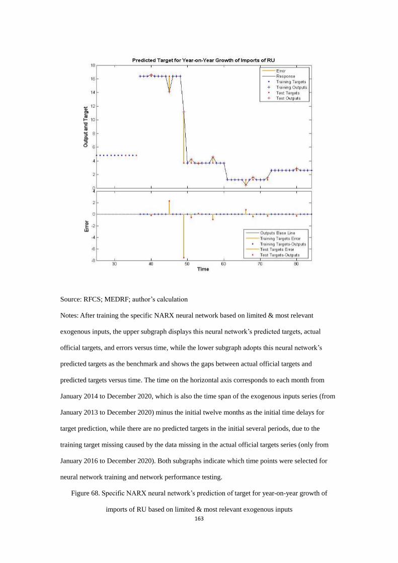
163

Source: RFCS; MEDRF; author’s calculation

Notes: After training the specific NARX neural network based on limited & most relevant

exogenous inputs, the upper subgraph displays this neural network’s predicted targets, actual

official targets, and errors versus time, while the lower subgraph adopts this neural network’s

predicted targets as the benchmark and shows the gaps between actual official targets and

predicted targets versus time. The time on the horizontal axis corresponds to each month from

January 2014 to December 2020, which is also the time span of the exogenous inputs series (from

January 2013 to December 2020) minus the initial twelve months as the initial time delays for

target prediction, while there are no predicted targets in the initial several periods, due to the

training target missing caused by the data missing in the actual official targets series (only from

January 2016 to December 2020). Both subgraphs indicate which time points were selected for

neural network training and network performance testing.

Figure 68. Specific NARX neural network’s prediction of target for year-on-year growth of

imports of RU based on limited & most relevant exogenous inputs

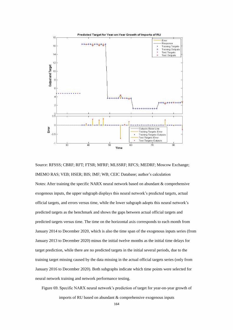
164

Source: RFSSS; CBRF; RFT; FTSR; MFRF; MLSSRF; RFCS; MEDRF; Moscow Exchange;

IMEMO RAS; VEB; HSER; BIS; IMF; WB; CEIC Database; author’s calculation

Notes: After training the specific NARX neural network based on abundant & comprehensive

exogenous inputs, the upper subgraph displays this neural network’s predicted targets, actual

official targets, and errors versus time, while the lower subgraph adopts this neural network’s

predicted targets as the benchmark and shows the gaps between actual official targets and

predicted targets versus time. The time on the horizontal axis corresponds to each month from

January 2014 to December 2020, which is also the time span of the exogenous inputs series (from

January 2013 to December 2020) minus the initial twelve months as the initial time delays for

target prediction, while there are no predicted targets in the initial several periods, due to the

training target missing caused by the data missing in the actual official targets series (only from

January 2016 to December 2020). Both subgraphs indicate which time points were selected for

neural network training and network performance testing.

Figure 69. Specific NARX neural network’s prediction of target for year-on-year growth of

imports of RU based on abundant & comprehensive exogenous inputs

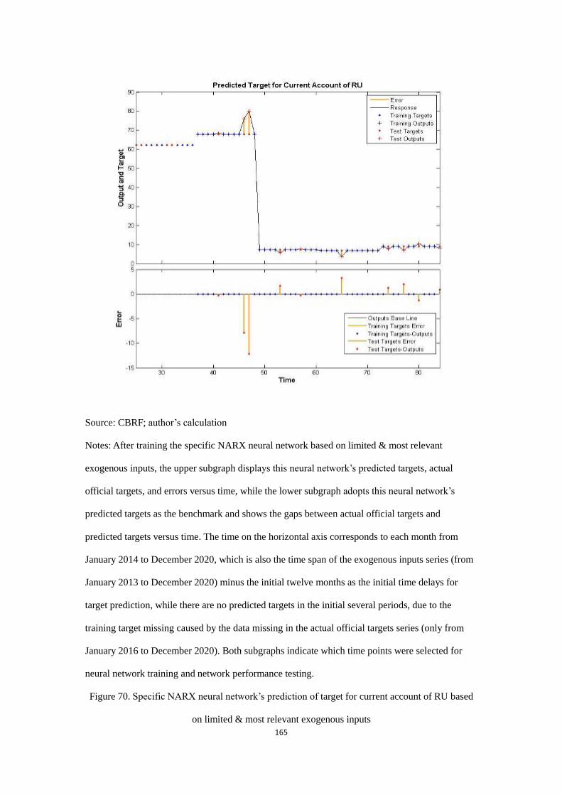
165

Source: CBRF; author’s calculation

Notes: After training the specific NARX neural network based on limited & most relevant

exogenous inputs, the upper subgraph displays this neural network’s predicted targets, actual

official targets, and errors versus time, while the lower subgraph adopts this neural network’s

predicted targets as the benchmark and shows the gaps between actual official targets and

predicted targets versus time. The time on the horizontal axis corresponds to each month from

January 2014 to December 2020, which is also the time span of the exogenous inputs series (from

January 2013 to December 2020) minus the initial twelve months as the initial time delays for

target prediction, while there are no predicted targets in the initial several periods, due to the

training target missing caused by the data missing in the actual official targets series (only from

January 2016 to December 2020). Both subgraphs indicate which time points were selected for

neural network training and network performance testing.

Figure 70. Specific NARX neural network’s prediction of target for current account of RU based

on limited & most relevant exogenous inputs

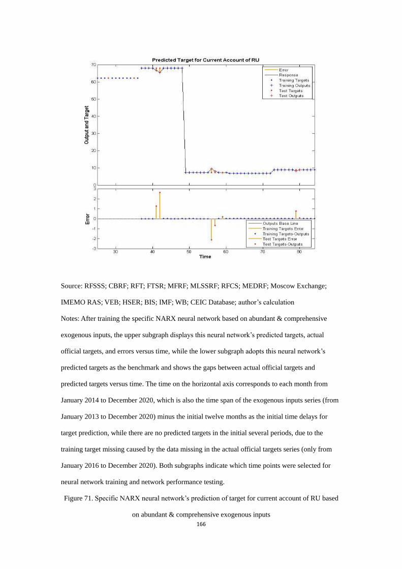
166

Source: RFSSS; CBRF; RFT; FTSR; MFRF; MLSSRF; RFCS; MEDRF; Moscow Exchange;

IMEMO RAS; VEB; HSER; BIS; IMF; WB; CEIC Database; author’s calculation

Notes: After training the specific NARX neural network based on abundant & comprehensive

exogenous inputs, the upper subgraph displays this neural network’s predicted targets, actual

official targets, and errors versus time, while the lower subgraph adopts this neural network’s

predicted targets as the benchmark and shows the gaps between actual official targets and

predicted targets versus time. The time on the horizontal axis corresponds to each month from

January 2014 to December 2020, which is also the time span of the exogenous inputs series (from

January 2013 to December 2020) minus the initial twelve months as the initial time delays for

target prediction, while there are no predicted targets in the initial several periods, due to the

training target missing caused by the data missing in the actual official targets series (only from

January 2016 to December 2020). Both subgraphs indicate which time points were selected for

neural network training and network performance testing.

Figure 71. Specific NARX neural network’s prediction of target for current account of RU based

on abundant & comprehensive exogenous inputs

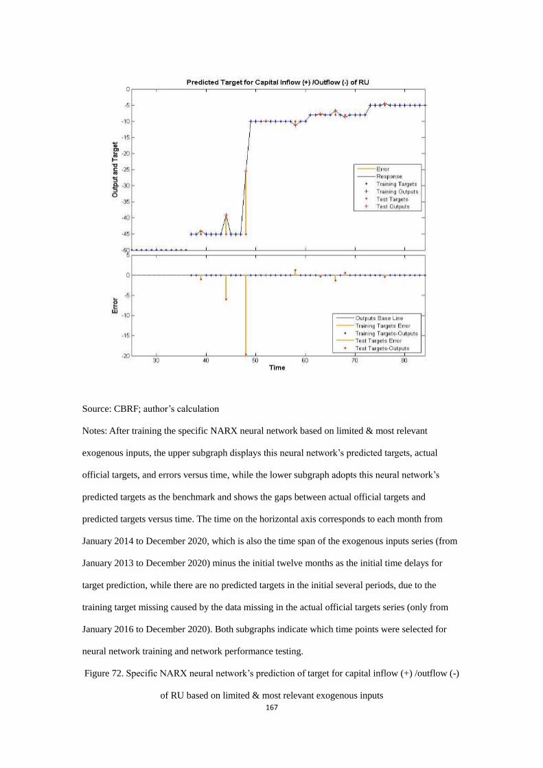
167

Source: CBRF; author’s calculation

Notes: After training the specific NARX neural network based on limited & most relevant

exogenous inputs, the upper subgraph displays this neural network’s predicted targets, actual

official targets, and errors versus time, while the lower subgraph adopts this neural network’s

predicted targets as the benchmark and shows the gaps between actual official targets and

predicted targets versus time. The time on the horizontal axis corresponds to each month from

January 2014 to December 2020, which is also the time span of the exogenous inputs series (from

January 2013 to December 2020) minus the initial twelve months as the initial time delays for

target prediction, while there are no predicted targets in the initial several periods, due to the

training target missing caused by the data missing in the actual official targets series (only from

January 2016 to December 2020). Both subgraphs indicate which time points were selected for

neural network training and network performance testing.

Figure 72. Specific NARX neural network’s prediction of target for capital inflow (+) /outflow (-)

of RU based on limited & most relevant exogenous inputs

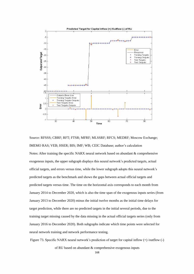
168

Source: RFSSS; CBRF; RFT; FTSR; MFRF; MLSSRF; RFCS; MEDRF; Moscow Exchange;

IMEMO RAS; VEB; HSER; BIS; IMF; WB; CEIC Database; author’s calculation

Notes: After training the specific NARX neural network based on abundant & comprehensive

exogenous inputs, the upper subgraph displays this neural network’s predicted targets, actual

official targets, and errors versus time, while the lower subgraph adopts this neural network’s

predicted targets as the benchmark and shows the gaps between actual official targets and

predicted targets versus time. The time on the horizontal axis corresponds to each month from

January 2014 to December 2020, which is also the time span of the exogenous inputs series (from

January 2013 to December 2020) minus the initial twelve months as the initial time delays for

target prediction, while there are no predicted targets in the initial several periods, due to the

training target missing caused by the data missing in the actual official targets series (only from

January 2016 to December 2020). Both subgraphs indicate which time points were selected for

neural network training and network performance testing.

Figure 73. Specific NARX neural network’s prediction of target for capital inflow (+) /outflow (-)

of RU based on abundant & comprehensive exogenous inputs

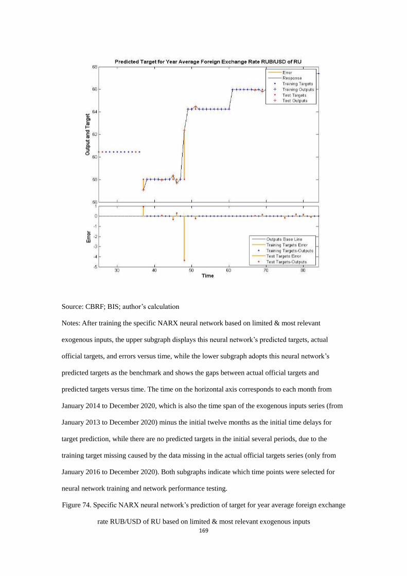
169

Source: CBRF; BIS; author’s calculation

Notes: After training the specific NARX neural network based on limited & most relevant

exogenous inputs, the upper subgraph displays this neural network’s predicted targets, actual

official targets, and errors versus time, while the lower subgraph adopts this neural network’s

predicted targets as the benchmark and shows the gaps between actual official targets and

predicted targets versus time. The time on the horizontal axis corresponds to each month from

January 2014 to December 2020, which is also the time span of the exogenous inputs series (from

January 2013 to December 2020) minus the initial twelve months as the initial time delays for

target prediction, while there are no predicted targets in the initial several periods, due to the

training target missing caused by the data missing in the actual official targets series (only from

January 2016 to December 2020). Both subgraphs indicate which time points were selected for

neural network training and network performance testing.

Figure 74. Specific NARX neural network’s prediction of target for year average foreign exchange

rate RUB/USD of RU based on limited & most relevant exogenous inputs

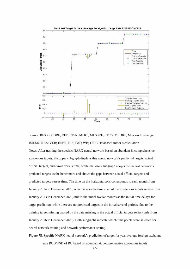
170

Source: RFSSS; CBRF; RFT; FTSR; MFRF; MLSSRF; RFCS; MEDRF; Moscow Exchange;

IMEMO RAS; VEB; HSER; BIS; IMF; WB; CEIC Database; author’s calculation

Notes: After training the specific NARX neural network based on abundant & comprehensive

exogenous inputs, the upper subgraph displays this neural network’s predicted targets, actual

official targets, and errors versus time, while the lower subgraph adopts this neural network’s

predicted targets as the benchmark and shows the gaps between actual official targets and

predicted targets versus time. The time on the horizontal axis corresponds to each month from

January 2014 to December 2020, which is also the time span of the exogenous inputs series (from

January 2013 to December 2020) minus the initial twelve months as the initial time delays for

target prediction, while there are no predicted targets in the initial several periods, due to the

training target missing caused by the data missing in the actual official targets series (only from

January 2016 to December 2020). Both subgraphs indicate which time points were selected for

neural network training and network performance testing.

Figure 75. Specific NARX neural network’s prediction of target for year average foreign exchange

rate RUB/USD of RU based on abundant & comprehensive exogenous inputs

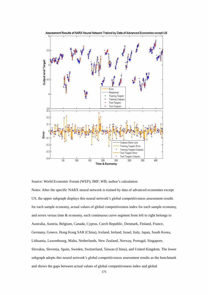
171

Source: World Economic Forum (WEF); IMF; WB; author’s calculation

Notes: After the specific NARX neural network is trained by data of advanced economies except

US, the upper subgraph displays this neural network’s global competitiveness assessment results

for each sample economy, actual values of global competitiveness index for each sample economy,

and errors versus time & economy, each continuous curve segment from left to right belongs to

Australia, Austria, Belgium, Canada, Cyprus, Czech Republic, Denmark, Finland, France,

Germany, Greece, Hong Kong SAR (China), Iceland, Ireland, Israel, Italy, Japan, South Korea,

Lithuania, Luxembourg, Malta, Netherlands, New Zealand, Norway, Portugal, Singapore,

Slovakia, Slovenia, Spain, Sweden, Switzerland, Taiwan (China), and United Kingdom. The lower

subgraph adopts this neural network’s global competitiveness assessment results as the benchmark

and shows the gaps between actual values of global competitiveness index and global

172

competitiveness assessment results versus time & economy. The time & economy on the

horizontal axis corresponds to each year from 2008 to 2017 (the time span of the exogenous inputs

series minus the initial two years as the initial time delays for assessment) for each sample

economy. Both subgraphs indicate which time points were selected for neural network training

and network performance testing.

Figure 76. Each sample economy’s global competitiveness assessment results from specific

NARX neural network trained by data of advanced economies except US

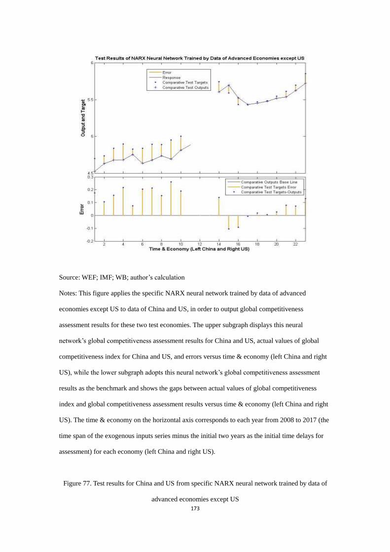
173

Source: WEF; IMF; WB; author’s calculation

Notes: This figure applies the specific NARX neural network trained by data of advanced

economies except US to data of China and US, in order to output global competitiveness

assessment results for these two test economies. The upper subgraph displays this neural

network’s global competitiveness assessment results for China and US, actual values of global

competitiveness index for China and US, and errors versus time & economy (left China and right

US), while the lower subgraph adopts this neural network’s global competitiveness assessment

results as the benchmark and shows the gaps between actual values of global competitiveness

index and global competitiveness assessment results versus time & economy (left China and right

US). The time & economy on the horizontal axis corresponds to each year from 2008 to 2017 (the

time span of the exogenous inputs series minus the initial two years as the initial time delays for

assessment) for each economy (left China and right US).

Figure 77. Test results for China and US from specific NARX neural network trained by data of

advanced economies except US

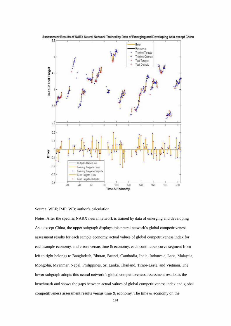
174

Source: WEF; IMF; WB; author’s calculation

Notes: After the specific NARX neural network is trained by data of emerging and developing

Asia except China, the upper subgraph displays this neural network’s global competitiveness

assessment results for each sample economy, actual values of global competitiveness index for

each sample economy, and errors versus time & economy, each continuous curve segment from

left to right belongs to Bangladesh, Bhutan, Brunei, Cambodia, India, Indonesia, Laos, Malaysia,

Mongolia, Myanmar, Nepal, Philippines, Sri Lanka, Thailand, Timor-Leste, and Vietnam. The

lower subgraph adopts this neural network’s global competitiveness assessment results as the

benchmark and shows the gaps between actual values of global competitiveness index and global

competitiveness assessment results versus time & economy. The time & economy on the

175

horizontal axis corresponds to each year from 2008 to 2017 (the time span of the exogenous inputs

series minus the initial two years as the initial time delays for assessment) for each sample

economy. Both subgraphs indicate which time points were selected for neural network training

and network performance testing.

Figure 78. Each sample economy’s global competitiveness assessment results from specific

NARX neural network trained by data of emerging and developing Asia except China

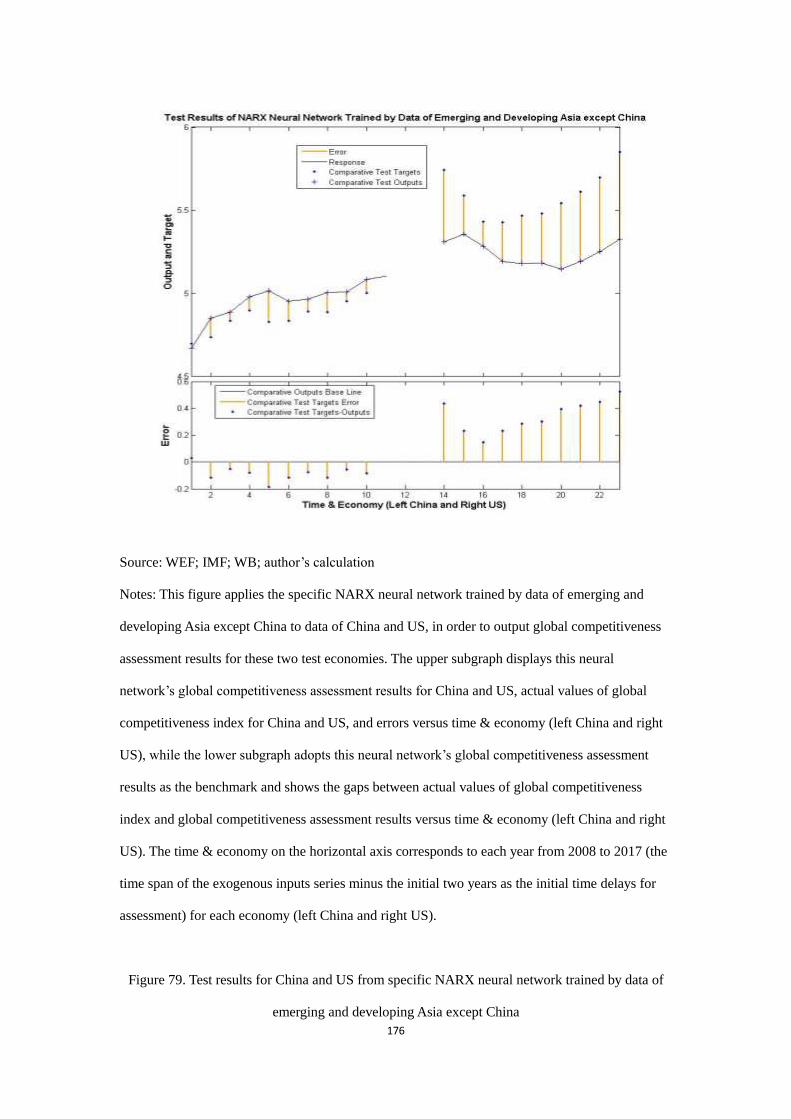
176

Source: WEF; IMF; WB; author’s calculation

Notes: This figure applies the specific NARX neural network trained by data of emerging and

developing Asia except China to data of China and US, in order to output global competitiveness

assessment results for these two test economies. The upper subgraph displays this neural

network’s global competitiveness assessment results for China and US, actual values of global

competitiveness index for China and US, and errors versus time & economy (left China and right

US), while the lower subgraph adopts this neural network’s global competitiveness assessment

results as the benchmark and shows the gaps between actual values of global competitiveness

index and global competitiveness assessment results versus time & economy (left China and right

US). The time & economy on the horizontal axis corresponds to each year from 2008 to 2017 (the

time span of the exogenous inputs series minus the initial two years as the initial time delays for

assessment) for each economy (left China and right US).

Figure 79. Test results for China and US from specific NARX neural network trained by data of

emerging and developing Asia except China

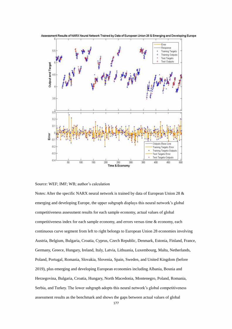
177

Source: WEF; IMF; WB; author’s calculation

Notes: After the specific NARX neural network is trained by data of European Union 28 &

emerging and developing Europe, the upper subgraph displays this neural network’s global

competitiveness assessment results for each sample economy, actual values of global

competitiveness index for each sample economy, and errors versus time & economy, each

continuous curve segment from left to right belongs to European Union 28 economies involving

Austria, Belgium, Bulgaria, Croatia, Cyprus, Czech Republic, Denmark, Estonia, Finland, France,

Germany, Greece, Hungary, Ireland, Italy, Latvia, Lithuania, Luxembourg, Malta, Netherlands,

Poland, Portugal, Romania, Slovakia, Slovenia, Spain, Sweden, and United Kingdom (before

2019), plus emerging and developing European economies including Albania, Bosnia and

Herzegovina, Bulgaria, Croatia, Hungary, North Macedonia, Montenegro, Poland, Romania,

Serbia, and Turkey. The lower subgraph adopts this neural network’s global competitiveness

assessment results as the benchmark and shows the gaps between actual values of global

178

competitiveness index and global competitiveness assessment results versus time & economy. The

time & economy on the horizontal axis corresponds to each year from 2008 to 2017 (the time span

of the exogenous inputs series minus the initial two years as the initial time delays for assessment)

for each sample economy. Both subgraphs indicate which time points were selected for neural

network training and network performance testing.

Figure 80. Each sample economy’s global competitiveness assessment results from specific

NARX neural network trained by data of European Union 28 & emerging and developing Europe

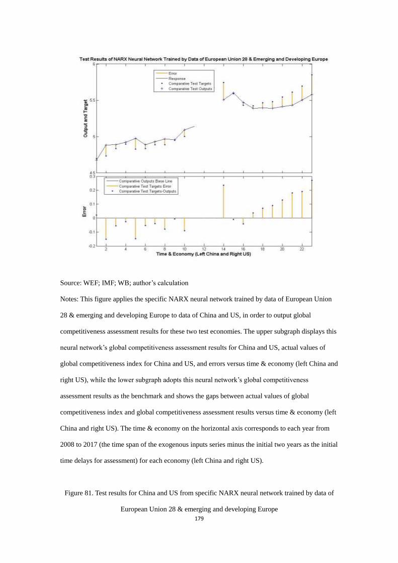
179

Source: WEF; IMF; WB; author’s calculation

Notes: This figure applies the specific NARX neural network trained by data of European Union

28 & emerging and developing Europe to data of China and US, in order to output global

competitiveness assessment results for these two test economies. The upper subgraph displays this

neural network’s global competitiveness assessment results for China and US, actual values of

global competitiveness index for China and US, and errors versus time & economy (left China and

right US), while the lower subgraph adopts this neural network’s global competitiveness

assessment results as the benchmark and shows the gaps between actual values of global

competitiveness index and global competitiveness assessment results versus time & economy (left

China and right US). The time & economy on the horizontal axis corresponds to each year from

2008 to 2017 (the time span of the exogenous inputs series minus the initial two years as the initial

time delays for assessment) for each economy (left China and right US).

Figure 81. Test results for China and US from specific NARX neural network trained by data of

European Union 28 & emerging and developing Europe