Absorption of Shocks in Nonlinear

Autoregressive Models

Dick van Dijk a,∗, Philip Hans Franses a H. Peter Boswijk b

aEconometric Institute, Erasmus University Rotterdam, P.O. Box 1738, NL-3000

DR Rotterdam, The Netherlands

bDepartment of Quantitative Economics, University of Amsterdam, Roetersstraat

11, NL-1018 WB Amsterdam, The Netherlands

Abstract

It generally is difficult, if not impossible, to fully understand and interpret nonlin-ear time series models by considering the estimated values of the model parametersonly. To shed light on the characteristics and implications of a nonlinear model itcan then be useful to consider the effects of shocks on the future patterns of thetime series variable. Most interest in such impulse response analysis has concen-trated on measuring the persistence of shocks, or the magnitude of their (ultimate)effect. A framework is developed and implemented that is useful for measuring therate at which this final effect is attained, or the rate of absorption of shocks. It isshown that the absorption rate can be used to examine whether the propagationof different types of shocks, such as positive and negative shocks or large and smallshocks follows different patterns. The nonlinear floor-and-ceiling model for US out-put growth is used to illustrate the various concepts. The presence of substantialasymmetries in both persistence and absorption of shocks is documented, with in-teresting differences arising across magnitudes of shocks and across regimes in themodel. Furthermore, it appears that asymmetry became much less pronounced dueto a large decline in output volatility in the 1980s.

Key words: impulse response, half-life, asymmetry, regime-switching models.

∗ Corresponding author. Tel.: +31-10-4081263; fax: +31-10-4089162Email addresses: djvandijk@few.eur.nl (Dick van Dijk),

franses@few.eur.nl (Philip Hans Franses), H.P.Boswijk@uva.nl (H. PeterBoswijk).

Preprint submitted to Elsevier Science 3 April 2006

1 Introduction

Nonlinear time series models are becoming increasingly popular in empiri-cal macroeconomics and empirical finance for describing and forecasting vari-ables such as output, (un)employment, stock returns and interest rates, seeGranger and Terasvirta (1993) and Franses and van Dijk (2000) for reviews.Examples of often considered models are the threshold autoregressive [TAR]model, see Tong (1990), the smooth transition autoregressive [STAR] model,see Chan and Tong (1986), Terasvirta (1994) and van Dijk, Terasvirta andFranses (2002), the Markov-Switching model put forward in Hamilton (1989),and the Artificial Neural Network [ANN] model advocated by Kuan and White(1994), among others. A key feature of these (and other) nonlinear time seriesmodels is that they assume that the model structure (lag length, parameters,variance) experiences occasional changes or, put differently, they assume thepresence of different regimes. Hence, these models can, for example, describeasymmetric business cycle behavior as observed in output and unemployment,or different behavior in different states of the financial market (for example,in bull and bear markets) as observed in stock returns and interest rates.

A common property of many of these (univariate) nonlinear models (and thisholds true even more so for their multivariate counterparts) is that only con-sidering (estimates of) the model parameters generally is not sufficient to com-pletely grasp the implied properties of time series generated by the model. Putdifferently, it is difficult to interpret a specific nonlinear model and to under-stand why it is useful in a particular application. Therefore, to shed lighton the characteristics of a nonlinear model it often is useful to consider theeffects of shocks on the future patterns of the time series variable. Impulseresponse functions provide a convenient tool for measuring such effects. Re-cent applications of impulse response analysis in nonlinear models in empiricalmacroeconomics and finance can be found in Weise (1999), Balke (2000), Du-four and Engle (2000), Taylor and Peel (2000), Altissimo and Violante (2001),Taylor, Peel and Sarno (2001), Balke, Brown and Yucel (2002), Skalin andTerasvirta (2002), Atanasova (2003), Chen, Tsai and Wu (2004), Dufrenot,Mignon and Peguin-Feissolle (2004), Grier et al. (2004), and Camacho (2005),among others.

Most applications of impulse response analysis concentrate on measuring thepersistence of shocks, indicated by the magnitude of their (ultimate) effecton the time series variable. Interestingly, far less attention typically is givento measuring the rate at which this final effect is attained, that is, how fastshocks are ‘absorbed’ by a time series. Due to the properties of impulse re-sponses in linear models, they can be used straightforwardly to gain insightin this rate of absorption of shocks as well, see, for example, Lutkepohl (2005)for a discussion of impulse response functions in linear models. However, im-

2

pulse response analysis in nonlinear models is more complicated, as discussedat length in Gallant, Rossi and Tauchen (1993), Koop, Pesaran and Potter(1996), and Potter (2000). The complications arise because in nonlinear mod-els (1) the effect of a shock depends on the history of the time series up tothe point where the shock occurs, (2) the effect of a shock need not be pro-portional to its size and (3) the effect of a shock depends on shocks occurringin periods between the moment at which the impulse occurs and the momentat which the response is measured. Because of these properties of impulseresponses, assessing the absorption time of shocks in nonlinear models alsois more involved, as will become clear below. In this paper we develop andimplement a framework that can be used for measuring and analyzing absorp-tion of shocks in nonlinear models. Among others, we demonstrate that ourabsorption measure can be used to address relevant questions such as

(1) Are positive and negative shocks absorbed at the same rate? Are shocksof different magnitudes absorbed at the same rate?

(2) Does the rate of absorption of shocks depend on the initial values or thehistory of the time series?

(3) Are shocks absorbed at the same rate by the different components of amultivariate time series?

(4) Are shocks absorbed at the same rate by linear combinations of the com-ponents in a multivariate time series and by the individual componentsthemselves?

It should be stressed at the outset that our absorption measure should notbe considered as a substitute for conventional impulse response analysis andpersistence measures but rather as a complement. Our absorption measureallows one to obtain a more complete picture of the propagation mechanismof a nonlinear model, as it can highlight interesting asymmetry properties ofshocks to economic time series different from the ones that are revealed byimpulse response functions as such.

Finally, an alternative approach to absorption is developed by Lee and Pesaran(1993) and Pesaran and Shin (1996). They examine the time profile of theeffect of shocks by means of so-called ‘persistence profiles’, defined as thedifference between the conditional variances of n-step and (n − 1)-step aheadforecasts, viewed as a function of n. Also see Galbraith (2003) on the relatedconcept of ‘content horizons’, defined as the ratio of the conditional varianceof n-step ahead forecasts and the unconditional variance of the time series ofinterest.

Our paper proceeds as follows. In Section 2, we briefly review the main aspectsof impulse response analysis in nonlinear time series models and the general-ized impulse response functions introduced by Koop et al. (1996). In Section3, we develop our measure of absorption of shocks. To facilitate the under-

3

standing of the concept of absorption, we concentrate on univariate modelsfirst. In this section we also demonstrate how to address the question of asym-metric absorption, that is the question whether positive and negative shocksare absorbed differently. In Section 4, we generalize our absorption measureto multivariate models. Particular attention is given to the question whethershocks are absorbed at the same rate by the different components of a mul-tivariate time series. We also outline how to measure absorption for a linearcombination of the components of a multivariate time series. In Section 5,we discuss an empirical application to quarterly US GDP growth rates us-ing the floor-and-ceiling model of Pesaran and Potter (1997). We documentthe presence of substantial asymmetries in both persistence and absorption ofshocks, with interesting differences arising across magnitudes of shocks andacross regimes in the model. Furthermore, it appears that asymmetry becamemuch less pronounced due to a large decline in output volatility in the 1980s.Finally, Section 6 contains some concluding remarks.

2 Preliminaries

Consider the multivariate nonlinear autoregressive time series model

Yt = F (Yt−1, . . . , Yt−p; θ) + Vt, (1)

where Yt = (Y1t, . . . , Ykt)′ is a (k × 1) random vector, F (·) is a known func-

tion that depends on the (q × 1) parameter vector θ, Vt = (V1t, . . . , Vkt)′ is a

(k× 1) vector of random disturbances with E[Vt|Ωt−1] = 0 and E[VtV′t |Ωt−1] =

H(Yt−1, . . . , Yt−r; ξ), where the (k×k) conditional covariance matrix H(Yt−1, . . . , Yt−r; ξ) ≡Ht = Ht,ij, i, j = 1, . . . , k depends on the (s × 1) parameter vector ξ.

Throughout, we use upper-case letters to denote random variables and lower-case letters to denote realizations of those random variables. For example, yt

and vt are realizations of Yt and Vt, respectively. The ‘history’ of the processup to t−1, which is the information set used to forecast future values of Yt, isdenoted as Ωt−1, with corresponding realizations denoted as ωt−1. Because thenonlinear model (1) is Markov of order max(p, r), it suffices to take Ωt−1 =Yt−1, . . . , Yt−max(p,r).

2.1 Impulse response functions

Impulse response functions are meant to provide a measure of the effect ofa shock vt occurring at time t on the time series after n periods, that is onYt+n for n ≥ 0. The impulse response measure that is commonly used in the

4

analysis of linear models is defined as the difference between two realizations ofYt+n. Both realizations start from the same history ωt−1, but in one realizationthe process is hit by a shock of size vt at time t, while in the other realizationno shock occurs at time t. Furthermore, all shocks in intermediate periodsbetween t and t + n are set equal to zero in both realizations, such that thetraditional impulse response function [TI] is given by

TIY (n, vt, ωt−1) = E[Yt+n|Vt = vt, Vt+1 = . . . = Vt+n = 0, ωt−1]−E[Yt+n|Vt = 0, Vt+1 = . . . = Vt+n = 0, ωt−1], (2)

for n = 0, 1, 2, . . .. The second realization usually is called the benchmarkprofile.

This traditional impulse response function has several convenient proper-ties in case the specification for the conditional mean F (Yt−1, . . . , Yt−p; θ)in (1) is linear. First, it is symmetric in the sense that a shock of magni-tude −vt has exactly the opposite effect as a shock of magnitude +vt, that isTIY (n, vt, ωt−1) = −TIY (n,−vt, ωt−1). Furthermore, it might be called linear,in the sense that the impulse response is proportional to the magnitude of theshock, that is TIY (n, a vt, ωt−1) = aTIY (n, vt, ωt−1) for all a 6= 0. Third, theimpulse response is history independent as it does not depend on the particu-lar history ωt−1, that is TIY (n, vt, ω

′t−1) = TIY (n, vt, ωt−1) for all histories ωt−1

and ω′t−1. Finally, the impulse response is independent of the shocks that occur

in intermediate periods t + 1, . . . , t + n. Even though vt+1, . . . , vt+n are com-monly set equal to 0, as in (2), the value of TIY (n, vt, ωt−1) does not changeif other values were used instead (as long as the same values are used in thetwo realizations defining the impulse response function). For example, in theunivariate AR(1) model Yt = φYt−1 + Vt, it holds that TIY (n, vt, ωt−1) = φnvt,from which the properties mentioned above are immediately obvious.

In general, none of these properties continue to hold in nonlinear time seriesmodels. In nonlinear models, the impact at t + n of a shock that occurs attime t typically depends (1) on the history of the process up to the time theshock occurs, (2) on the sign and the size of the shock, and (3) on the shocksthat occur in intermediate periods t+1, . . . , t+n. The first property is closelyrelated to the observation that the accuracy of forecasts from nonlinear modelsdepends on the initial value, see Yao and Tong (1994) and Fan, Yao and Tong(1996), among others. Concerning the third property, the assumption thatno shocks occur in intermediate periods, as in the TI in (2), might give riseto quite misleading inference concerning the propagation mechanism of thenonlinear model, see Pesaran and Potter (1997) for an example.

The Generalized Impulse Response Function [GI], introduced by Koop et al.(1996), provides a natural and elegant solution to the complications involvedin impulse response analysis in nonlinear models. The GI for a specific shock

5

vt and history ωt−1 is defined as

GIY (n, vt, ωt−1) = E[Yt+n|Vt = vt, ωt−1] − E[Yt+n|ωt−1], (3)

for n = 0, 1, 2, . . .. In the GI, the expectation of Yt+n given that a shock vt

occurs at time t is conditioned only on the history and on this shock. Put dif-ferently, the problem of handling shocks occurring in intermediate time periodsis dealt with by averaging them out. Given this choice, the natural benchmarkprofile for the impulse response is the expectation of Yt+n conditional only onthe history of the process ωt−1. Thus, in the benchmark profile the currentshock is averaged out as well. It is straightforward to show that for linearmodels the GI in (3) is equivalent to the traditional impulse response in (2).

The GI as defined in (3) is a function of vt and ωt−1, which are realizationsof the random variables Vt and Ωt−1. Koop et al. (1996) stress that henceGIY (n, vt, ωt−1) itself is a realization of the random variable given by

GIY (n, Vt, Ωt−1) = E[Yt+n|Vt, Ωt−1] − E[Yt+n|Ωt−1]. (4)

Using this interpretation of the GI as a random variable, various conditionalversions can be defined that are of potential interest. For example, one mightconsider a particular history ωt−1 and treat the GI as a random variable interms of the shock Vt only, that is,

GIY (n, Vt, ωt−1) = E[Yt+n|Vt, ωt−1] − E[Yt+n|ωt−1]. (5)

Alternatively, one could reverse the role of the shock and the history by fixingthe shock at Vt = vt and consider the GI as a random variable in terms ofthe history Ωt−1 only. In general, one might examine the GI conditional on asubset S of shocks and a subset H of histories, that is,

GIY (n,S,H) = E[Yt+n|Vt ∈ S, Ωt−1 ∈ H] − E[Yt+n|Ωt−1 ∈ H]. (6)

For example, one might condition on all histories such that Yt−1 ≤ 0 andconsider only negative shocks.

Note that as for nonlinear models analytic expressions for the conditional ex-pectations involved in the GI in (3) and (4) usually are not available, stochasticsimulation should be used to obtain estimates of the impulse response mea-sures. See Koop et al. (1996) for a detailed description of the relevant tech-niques. Finally, it is useful to note that the shock- and history-specific impulseresponse measure GIY (n, vt, ωt−1) in (3) can still be interpreted as a randomvariable if parameter uncertainty is taken into account as an additional sourceof randomness. In that case, Bayesian techniques are convenient to constructthe distribution of the impulse response, as discussed in Koop (1996).

The two aspects of impulse responses that appear to be of most interest are (1)the final response to an impulse, and (2) the rate at which this final response

6

is attained. Traditionally, most attention has been given to the first element,usually referred to as persistence. In the present paper we focus on the secondaspect, which we call absorption. Before we proceed to discuss how absorptioncan be measured in the next section, we summarize how persistence of shockscan be assessed by means of the GI. This section then closes with some remarkson how to determine whether the response to positive and negative shocks isasymmetric.

2.2 Measuring persistence of shocks

A shock vt is said to be transient at history ωt−1 if in the long run the shockdoes not affect the pattern of the time series, that is, if GIY (n, vt, ωt−1) becomesequal to 0 as the horizon n goes to infinity. If this is not the case, the shockis said to be persistent. The final impulse response for a specific shock andhistory can be obtained as

GI∞Y (vt, ωt−1) = limn→∞GIY (n, vt, ωt−1), (7)

if this limit exists. In practice, the final impulse response GI∞Y (vt, ωt−1) can beestimated by GIY (nmax, vt, ωt−1) for certain large nmax.

Potter (1995a) and Koop et al. (1996) suggest that the dispersion of the distri-bution of GIY (n, Vt, Ωt−1) at finite horizons n can be interpreted as a measureof persistence of shocks. It is intuitively clear that if a time series process isstationary and ergodic, the effect of all shocks eventually becomes zero for allpossible histories of the process. Hence, GI∞Y (vt, ωt−1) in (7) is equal to zero forall choices of vt and ωt−1 or, put differently, the distribution of GIY (n, Vt, Ωt−1)collapses to a spike at 0 as n → ∞. By contrast, for nonstationary time seriesthe dispersion of the distribution of GIY (n, Vt, Ωt−1) is positive for all n. Con-ditional versions of the GI are particularly suited to assess the persistence ofshocks. For example, one might compare the dispersion of the distributions ofGIs conditional on positive and negative shocks to determine whether negativeshocks are more persistent than positive ones, or vice versa. A potential prob-lem with this approach is that no unambiguous measure of dispersion exists,although the notion of second-order stochastic dominance might be useful inthis context, see Potter (2000).

2.3 Measuring asymmetric impulse response

One possible use of the GI is to examine asymmetry in the effects of positiveand negative shocks. Potter (1994) defines a measure of asymmetric responseto a particular (positive) shock Vt = vt given a particular history ωt−1 as the

7

sum of the GI for this particular shock and the GI for the shock of the samemagnitude but with opposite sign, that is,

ASYY (n, vt, ωt−1) = GIY (n, vt, ωt−1) + GIY (n,−vt, ωt−1). (8)

As noted before, by taking into account parameter uncertainty as an additionalsource of randomness, GIY (n, vt, ωt−1), and hence ASYY (n, vt, ωt−1), can stillbe interpreted as a random variable. Potter (1995b) uses a straightforwardsimulation procedure to assess whether this shock- and history-specific asym-metry measure is significantly different from zero or not.

Alternatively, one could consider the distribution of the random asymmetrymeasure

ASYY (n, V +t , Ωt−1) = GIY (n, V +

t , Ωt−1) + GIY (n,−V +t , Ωt−1), (9)

where V +t = vt|vt > 0 indicates the set of all positive shocks. If posi-

tive and negative shocks induce the same response (but with opposite sign),ASYY (n, V +

t , Ωt−1) should be equal to zero almost surely. More generally, thedistribution of ASYY (n, V +

t , Ωt−1) may be used to infer the asymmetry proper-ties of the impulse response function GIY (n, Vt, Ωt−1). When this distributionhas mean (or median) equal to zero, shocks may be said to have a symmetriceffect on average. At the same time, the dispersion and skewness of this dis-tribution might be interpreted as measures of the asymmetry in the effects ofpositive and negative shocks.

3 Absorption of shocks in univariate models

Irrespective of whether shocks are persistent or not, it should be of interestto assess how fast innovations are absorbed, that is, the rate at which the GIapproaches the final response GI∞Y (vt, ωt−1). In this section we discuss howabsorption can be measured.

3.1 Definition of absorption

Suppose for the moment that Yt is a univariate time series. Define the indicatorfunction

IY (π, n, vt, ωt−1) ≡ I[|GIY (n, vt, ωt−1)−GI∞Y (vt, ωt−1)| ≤ π|vt−GI∞Y (vt, ωt−1)|],(10)

for certain π such that 0 ≤ π ≤ 1, where I[A] = 1 if the event A occurs and0 otherwise, and where it is assumed that the limit defining GI∞Y (vt, ωt−1) in

8

(7) exists. In words, the function IY (π, n, vt, ωt−1) is equal to 1 if the absolutedifference between the GI at horizon n and the ultimate response to the shockvt, as given by GI∞Y (vt, ωt−1), is less than or equal to a fraction π of theabsolute difference between the shock vt (which is equal to the initial impactof the shock or the GI at horizon 0) and the ultimate response. Put differently,IY (π, n, vt, ωt−1) = 1 if at least a fraction 1 − π of the difference between theinitial and ultimate effects of vt has been absorbed after n periods.

The ‘π-life’ or ‘π-absorption time’ of vt can now be defined as

NY (π, vt, ωt−1) =∞∑

m=0

(

1 −∞∏

n=m

IY (π, n, vt, ωt−1)

)

. (11)

In words, NY (π, vt, ωt−1) is the minimum horizon beyond which the differencebetween the impulse responses at all longer horizons and the ultimate responseis less than or equal to a fraction π of the difference between the initial impactand the ultimate response. That is, NY (π, vt, ωt−1) = n∗ if IY (π, n, vt, ωt−1) =1 for all n ≥ n∗ and IY (π, n∗ − 1, vt, ωt−1) = 0. The reason for not definingNY (π, vt, ωt−1) as the shortest horizon for which IY (π, n, vt, ωt−1) = 1 is thatthe GI need not approach the limit GI∞Y (vt, ωt−1) monotonically. Hence, itmay occur that IY (π, n, vt, ωt−1) = 1 and IY (π, n + j, vt, ωt−1) = 0 for certainj > 0.

Just like the shock- and history-specific GI in (3) can be regarded as a real-ization of the random variable GIY (n, Vt, Ωt−1) in (4), the π-absorption timeNY (π, vt, ωt−1) in (11) can be regarded as a realization of the random variable

NY (π, Vt, Ωt−1) =∞∑

m=0

(

1 −∞∏

n=m

IY (π, n, Vt, Ωt−1)

)

, (12)

where the random indicator function IY (π, n, Vt, Ωt−1) is defined as

IY (π, n, Vt, Ωt−1) ≡ I[|GIY (n, Vt, Ωt−1)−GI∞Y (Vt, Ωt−1)| ≤ π|Vt−GI∞Y (Vt, Ωt−1)|].(13)

Conditional versions NY (π,S,H) for a particular subset S of shocks and asubset H of histories can be defined analogously in a straightforward manner.

It is useful to consider some basic properties of the absorption measure NY (π, vt, ωt−1),which can conveniently be illustrated by means of the linear AR(1) modelYt = φYt−1 + Vt with |φ| < 1. In this case GIY (n, vt, ωt−1) = φnvt, andGI∞Y (vt, ωt−1) = 0. Thus, IY (π, n, vt, ωt−1) = I[|φnvt| ≤ π|vt|], which is equalto 1 if |φn| = |φ|n ≤ π, or n ≤ ln(π)/ ln(|φ|). From (11) it then followsthat NY (π, vt, ωt−1) = ⌈ln(π)/ ln(|φ|)⌉, where ⌈z⌉ denotes the smallest integergreater than or equal to z. First, observe that NY (π, vt, ωt−1) is independent ofthe (sign and size of the) shock vt and of the history ωt−1 in this case. Corre-sponding with the properties of the GI, this applies to all linear models but it

9

no longer holds for nonlinear models. Second, given that IY (π, n, vt, ωt−1) = 1implies IY (π′, n, vt, ωt−1) = 1 for all 0 ≤ π < π′ ≤ 1, it follows from the defini-tion of the absorption measure in (11) that NY (π′, vt, ωt−1) ≤ NY (π, vt, ωt−1).That is, there is a negative relationship between the π-life and π. Third,the fact that NY (π, vt, ωt−1) is discrete implies that the absorption measurehas to be applied with some care. In particular, for a given single value ofπ, NY (π, vt, ωt−1) is not necessarily able to discriminate between processesthat have different persistence properties. Examining the absorption mea-sure for a range of values for π helps to remedy this. For example, in theAR(1) case, the π-absorption time for π = 0.50, which corresponds to theusual measure of the half-life of shocks, is equal to 2 for both φ = 0.6 andφ = 0.7. On the other hand, NY (π, vt, ωt−1) for π = 0.10 is equal to 5 and7 for φ = 0.6 and 0.7, respectively. Finally, notice that for a random walkYt = Yt−1 +Vt, GIY (n, vt, ωt−1) = vt for all n ≥ 0, so that IY (π, n, vt, ωt−1) = 1and NY (π, vt, ωt−1) = 0 in all cases. This follows from the fact that for a ran-dom walk the final effect of a shock is reached instantaneously upon impact.

When implementing the absorption measure NY (π, Vt, Ωt−1) in practice, a fi-nite horizon nmax has to be chosen both to approximate (11) and to approx-imate the ultimate impulse response GI∞Y (Vt, Ωt−1) necessary for computingthe indicator function IY (π, n, Vt, Ωt−1) in (13). It is advisable to set the trun-cation point nmax fairly large, in any case larger than the typical horizonsof interest. In addition, it is appropriate to perform some empirical checksto ensure that GIY (n, Vt, Ωt−1) is approximately equal to GIY (nmax, Vt, Ωt−1)for horizons n > nmax. This would also provide a rough idea of the existenceof the limit GI∞Y (Vt, Ωt−1), and of the accuracy of GIY (nmax, Vt, Ωt−1) as aproxy for the ultimate response. We illustrate this and other aspects involvedin the practical implementation of the absorption measure in the empiricalapplication in Section 5.

3.2 Measuring asymmetric absorption

Possible asymmetry in the absorption of positive and negative shocks can beexamined in a way similar to detecting asymmetry in impulse responses, asdiscussed in Section 2.3. For a specific shock vt and history ωt−1, a measure ofasymmetric absorption can be defined as the difference in π-absorption timesof vt and −vt, that is,

ASYNY (π, vt, ωt−1) = NY (π, vt, ωt−1) − NY (π,−vt, ωt−1). (14)

If vt has symmetric absorption at ωt−1, ASYNY (π, vt, ωt−1) = 0 for all valuesof π.

Note that symmetry in GIY (n, vt, ωt−1), that is, ASYY (n, vt, ωt−1) = 0 for all

10

n ≥ 0 in (8), implies symmetry in absorption, that is, ASYNY (π, vt, ωt−1) = 0for all π ∈ (0, 1). Interestingly, the reverse does not hold, that is, a shockcan have symmetric absorption but an asymmetric impulse response. Also,ASYNY (π, vt, ωt−1) 6= 0 for certain π ∈ (0, 1) implies that ASYY (n, vt, ωt−1) 6=0 for certain n ≥ 0, whereas the reverse need not hold.

As before, the asymmetry measure in (14) can be regarded as a realization ofthe random variable

ASYNY (π, V +t , Ωt−1) = NY (π, V +

t , Ωt−1) − NY (π,−V +t , Ωt−1), (15)

where V +t is the set of positive shocks, as defined just below (9). Obviously,

the asymmetry measure can also be defined for a subset S+ of positive shocksand a subset H of histories.

By taking into account parameter uncertainty, one can consider whether aspecific shock vt has symmetric absorption at a specific history ωt−1 by ex-amining whether ASYNY (π, vt, ωt−1) is significantly different from zero. Toassess whether the absorption of shocks in the set S for the set of histories His symmetric on average, we may test whether the mean of the distributionof ASYNY (π,S+,H) is equal to zero. This is complicated by the fact thatthe different realizations ASYNY (π, vt, ωt−1) used to estimate this distribu-tion are not independent across histories ωt−1. Hence, the standard error forthe mean of ASYNY (π,S+,H) is not equal to σASYNY (π,S+,H)/

√nSH, where

σASYNY (π,S+,H) is the standard deviation of ASYNY (π,S+,H) and nSH is thenumber of combinations of shocks vt and histories ωt−1 for which ASYNY (π, vt, ωt−1)is computed. Note however that the ASYNY (π, vt, ωt−1) are independent acrossshocks vt. Therefore, as a conservative standard error for the mean of ASYNY (π,S+,H)we suggest to use σASYNY (π,S+,H)/

√nS , where nS is the number of shocks vt

for which ASYNY (π, vt, ωt−1) is computed.

Alternatively, the asymmetry of the distribution of ASYNY (π,S+,H) can beassessed by means of confidence regions. Following Hyndman (1995), we con-sider three different 100 · (1 − α)% confidence regions:

(1) An interval symmetric around the mean

SAMα = (µASYNY (π,S+,H) − w, µASYNY (π,S+,H) + w),

where µASYNY (π,S+,H) is the mean of the asymmetry measure ASYNY (π,S+,H)and w is such that P (ASYNY (π,S+,H) ∈ SAMα) = 1 − α.

(2) The interval between the α/2 and (1−α/2) quantiles of the distributionof ASYNY (π,S+,H), denoted qα/2 and q1−α/2, respectively,

EQIα = (qα/2, q1−α/2).

11

(3) The highest-density region [HDR]

HDRα = ASYNY (π,S+,H) | g(ASYNY (π,S+,H)) ≥ gα, (16)

where g(·) is the density of its argument and gα is such that P (ASYNY (π,S+,H) ∈HDRα) = 1 − α.

For symmetric and unimodal distributions, these three regions are identical.For asymmetric or multimodal distributions they are not, see Hyndman (1995)for discussion and Chan and Tong (2004) for recent tests for multimodality. Inthe applications below, we report α∗, which is the minimum value of α ∈ (0, 1)such that 0 would not be included in the relevant confidence region and, hence,can be interpreted as the p-value for testing the hypothesis that the mean ofASYNY (π,S+,H) = 0. Note that the three confidence regions all providedifferent information. The interval symmetric around the mean indicates theposition of 0 relative to the mean of the distribution. The interval with equalquantiles in the tail indicates whether 0 is located in the tails or in the centralpart of the distribution. Finally, the HDR indicates the probability that theasymmetry measure is equal to 0.

4 Absorption of shocks in multivariate models

The concept of absorption can also be used to investigate the properties ofmultivariate nonlinear models. In this section, we first define the multivariateextension of the univariate absorption measure used so far. Next, we discusshow to measure whether shocks are absorbed at the same rate by the differentcomponents of a multivariate time series, which we call common absorption.

4.1 Definition of absorption in multivariate models

Extending the π-absorption time measure to multivariate models is fairlystraightforward. Following Pesaran and Shin (1998), we restrict attention tothe generalized impulse response measuring the effect of a shock in the j-thequation only. Consistent with the idea of GIs that irrelevant shocks are dealtwith by integrating out their effects, not only the shocks during intermediateperiods t + 1, . . . , t + n are averaged out, but shocks to the other equationsoccurring at time t as well. Hence, we have

GIY (n, vjt, ωt−1) = E[Yt+n|Vjt = vjt, ωt−1] − E[Yt+n|ωt−1]. (17)

The immediate effect of the shock is given by the impulse response at horizonn = 0, which is equal to GIY (0, vjt, ωt−1) = E[Vt|Vjt = vjt, ωt−1]. If conditional

12

upon the history ωt−1, Vt is normally distributed with covariance matrix ht, itcan be shown that

E[Vt|Vjt = vjt, ωt−1] = (ht,1j , ht,2j , . . . , ht,kj)′h−1

t,jjvjt = htejh−1t,jjvjt,

where ej is a (k×1) vector with unity as its j-th element and zeros elsewhere,see Pesaran and Shin (1998). Thus, the indicator function IYi

(π, n, vjt, ωt−1)now may be defined as

IYi(π, n, vjt, ωt−1) =

I[|GIYi(n, vjt, ωt−1) − GI∞Yi

(vjt, ωt−1)| ≤ π|ht,ijh−1t,jjvjt − GI∞Yi

(vjt, ωt−1)|].

The ‘π-life’ or ‘π-absorption time’ of vjt for Yi then can be defined as

NYi(π, vjt, ωt−1) =

∞∑

m=0

(

1 −∞∏

n=m

IYi(π, n, vjt, ωt−1)

)

. (18)

As in the univariate case, NYi(π, vjt, ωt−1) can be regarded as a realization of

the random variable

NYi(π, Vjt, Ωt−1) =

∞∑

m=0

(

1 −∞∏

n=m

IYi(π, n, Vjt, Ωt−1)

)

, (19)

where the random indicator function IYi(π, n, Vjt, Ωt−1) is obviously defined.

Similarly, one can define the asymmetry measure

ASYNYi(π, V +

jt , Ωt−1) = NYi(π, V +

jt , Ωt−1) − NYi(π,−V +

jt , Ωt−1), (20)

where V +jt = Vjt|Vjt > 0, which can be used to assess whether positive and

negative shocks are absorbed differently.

4.2 Measuring common absorption

In multivariate models, an additional question of interest is whether shocks areabsorbed at the same rate by different variables in the system. Define the ran-dom variable CNYi,Yl

(π, Vjt, Ωt−1) as the difference between the π-absorptiontimes of Yi and of Yl, that is

CNYi,Yl(π, Vjt, Ωt−1) = NYi

(π, Vjt, Ωt−1) − NYl(π, Vjt, Ωt−1). (21)

If shocks Vjt are absorbed at the same rate by Yi and Yl on average, CNYi,Yl(π, Vjt, Ωt−1)

should have a distribution with mean equal to zero.

Alternatively, one may ask whether there exists a linear combination β ′Y , fora certain (k × 1) vector β, for which the effects of shocks die out faster than

13

for the component series Yi, i = 1, . . . , k. If so, this linear combination can beviewed as a more stable variable as shocks last for a shorter period of time.From the definition of the GI given in (4) and elementary properties of theconditional expectations operator it follows that

GIβ′Y (n, Vjt, Ωt−1) = β ′GIY (n, Vjt, Ωt−1). (22)

Hence, the GI for a linear combination of the elements in Yt can be obtaineddirectly as the same linear combination of the GI of Yt. Note that such asimple relationship does not exist between the π-absorption times of a linearcombination and the absorption times of the elements of Yt. That is, in general

Nβ′Y (π, Vjt, Ωt−1) 6= β ′NY (π, Vjt, Ωt−1),

where NY (π, Vjt, Ωt−1) = (NY1(π, Vjt, Ωt−1), . . . , NYk(π, Vjt, Ωt−1))

′. It is how-ever straightforward to define the π-absorption time of β ′Yt as

Nβ′Y (π, Vjt, Ωt−1) =∞∑

m=0

(

1 −∞∏

n=m

Iβ′Y (π, n, Vjt, Ωt−1)

)

,

where the indicator function Iβ′Y (π, n, Vjt, Ωt−1) is defined as

Iβ′Y (π, n, Vjt, Ωt−1) =

I[|β ′(GIY (n, Vjt, Ωt−1)−GI∞Y (Vjt, Ωt−1))| ≤ π|β ′(htejh−1t,jjVjt−GI∞Y (Vjt, Ωt−1))|].

An alternative common absorption measure CANYi,Yl(π, Vjt, Ωt−1) can then be

defined as the difference of the π-absorption times of Yi and β ′Y , that is

CANYi,β′Y (π, Vjt, Ωt−1) = NYi(π, Vjt, Ωt−1)−Nβ′Y (π, Vjt, Ωt−1), i = 1, . . . , k.

(23)If shocks Vjt are not absorbed differently by the linear combination β ′Y thanby the individual series Yi on average, CANYi,β′Y (π, Vjt, Ωt−1) should have adistribution with mean equal to zero for all i = 1, . . . , k.

5 Impulse response and absorption in the floor-and-ceiling model

US output growth has been by far the most popular macro-economic appli-cation of nonlinear regime-switching time series models. In particular, follow-ing Hamilton (1989) many attempts have been made to describe the appar-ent asymmetric behavior over the business cycle in US output by means ofMarkov-Switching models, see Clements and Krolzig (2002) and Kim, Morley,and Piger (2005) for recent contributions. Alternatively, threshold and smoothtransition models have also been used for this purpose, see Potter (1995b) and

14

Terasvirta (1995), respectively. Here we consider the floor-and-ceiling modelof Pesaran and Potter (1997), which attempts to capture business cycle asym-metry by including ‘current-depth-of-recession’ and ‘overheating’ variables asadditional regressors in a linear autoregressive model for the growth rate ofoutput.

To develop the model, define the indicators Ft and Ct for the floor and ceilingregimes recursively as

Ft =

I[∆Yt < rF ] if Ft−1 = 0,

I[CDRt−1 + ∆Yt < 0] if Ft−1 = 1,(24)

Ct = I[Ft = 0]I[∆Yt > rC ]I[∆Yt−1 > rC ], (25)

where the current-depth-of-recession variable CDRt is defined as

CDRt =

(∆Yt − rF )Ft if Ft−1 = 0,

(CDRt−1 + ∆Yt)Ft if Ft−1 = 1,(26)

and the overheating variable OHt is given by

OHt = Ct(OHt−1 + ∆Yt − rC). (27)

The above definitions imply that the floor regime is entered whenever outputgrowth falls below the threshold rF . In that case CDRt measures the accu-mulated growth below rF since entering the floor regime. The floor regime isleft whenever this ‘growth deficit’ is eliminated and CDRt turns non-negative.Note that in case the floor threshold rF = 0, (26) with (24) reduces to thegap between the current value of output and its historical maximum value,that is CDRt = Yt − maxj≥0 Yt−j , as used by Beaudry and Koop (1993). Theceiling regime becomes active when output growth exceeds the threshold rC

in two consecutive quarters (and provided that the floor regime is not active).The overheating variable OHt then measures the accumulated growth over theceiling rC . The floor-and-ceiling model for output growth now is given by

φ(L)∆Yt = φ0 + θ1CDRt−1 + θ2OHt−1 + Vt, (28)

where φ(L) = 1−φ1L− . . .−φpLp is a lag polynomial of order p, with the lag

operator defined as LmYt = Yt−m for all m and ∆ = 1−L is the first-differenceoperator, E[Vt|Ωt−1] = 0, and the conditional variance of Vt is given by

E[V 2t |Ωt−1] ≡ Ht = (σ2

F Ft−1 + σ2CORCORt−1 + σ2

CCt−1)(1− σ2BI[t > τ ]), (29)

where the indicator for the corridor regime is defined as

CORt = I[Ft + Ct = 0].

15

Compared to the original model of Pesaran and Potter (1997), the conditionalvolatility specification in (29) is augmented with the term (1 − σ2

BI[t > τ ]).This is included to accommodate the large decline in output volatility thatoccurred during the 1980s, see McConnell and Perez-Quiros (2000), Stockand Watson (2003) and Sensier and van Dijk (2004), among others. Notethat we assume that this break affects volatility in all three regimes equally.Pesaran and Potter (1997) provide an extensive discussion and motivation ofthe floor-and-ceiling model, showing among others that it can be interpretedas a specific type of threshold model.

The floor-and-ceiling model is applied to quarterly observations on seasonallyadjusted real US GDP, from 1954:1-2004:4, expressed in annualized percent-age points. Following Pesaran and Potter (1997), we set p = 2 in (28). Wefix the date of the volatility break τ to be equal to 1984:1, as established byMcConnell and Perez-Quiros (2000) and Stock and Watson (2003). We esti-mate the model parameters with maximum likelihood, using a grid search overthe floor and ceiling thresholds rF and rC where we require that each of theregimes contains at least 10% of the observations. The resulting parameterestimates, with heteroskedasticity-consistent standard errors in parentheses,are given by φ0 = 1.205(0.153), φ1 = 0.310(0.006), φ2 = 0.314(0.006), θ1 =−0.524(0.050), θ2 = −0.072(0.002), σF = 5.280(0.645), σCOR = 4.095(0.113),σC = 3.740(0.150), σB = 0.554(0.002), rF = −2.775, and rC = 3.297. In theeffective estimation sample, 23, 120 and 58 observations are located in thefloor, corridor and ceiling regimes, respectively. The statistically significantnegative estimates of θ1 and θ2 indicate that the model implies the presenceof ‘dampening effects’. Given that CDRt is zero in the corridor and ceilingregimes and becomes negative in the floor regime, average growth increasessharply during recessions. Similarly, OHt is positive in the ceiling regime andequal to zero otherwise, such that average growth falls when the economy isoverheated. Finally, note that the estimate of σB indicates that volatility ofGDP growth has been substantially lower after 1984 than it was before.

We use impulse response analysis to examine whether the persistence and ab-sorption of shocks varies with the history of the time series, with the signof the shock and with its magnitude. In addition, we consider the effects ofthe volatility break in 1984:1 on these impulse response properties. For thispurpose, we compute two sets of impulse response functions GI∆Y (n, vt, ωt−1)for all 201 histories ωt−1 in the sample, for values of the normalized shockequal to vt/

√ht = 0,±0.1, . . . ,±2.9,±3, where ht denotes a realization of the

conditional variance Ht. For the first set of GIs, Ht is set equal to σ2F Ft−1 +

σ2CORCORt−1 + σ2

CCt−1, corresponding with the pre-break level of the condi-tional variance in (29), while for the second set of GIs, this is multiplied with(1 − σ2

B) such that Ht corresponds with the post-break conditional variances.The relevant histories consist of the growth rate in the two previous periodsand the lagged CDR and OH variables, that is Ωt−1 = ∆Yt−1, ∆Yt−2, CDRt−1, OHt−1.

16

GIs are computed for horizons n = 0, 1, . . . , nmax with nmax = 20, using thealgorithm outlined in Koop et al. (1996), with 50, 000 replications to averageout the effects of shocks occurring in intermediate periods, which are sampledfrom a normal distribution. Impulse responses for the log level of GNP areobtained by accumulating the impulse responses for the growth rate, that isGIY (n, vt, ωt−1) =

∑ni=0 GI∆Y (i, vt, ωt−1). At horizons beyond 20 quarters, the

impulse response GI∆Y (n, vt, ωt−1) is equal to 0 for virtually all shocks vt andωt−1. Hence, GIY (nmax, vt, ωt−1) forms a reliable estimate of the final impulseresponse GI∞Y (vt, ωt−1).

Figures 1 and 2 show distributions of GIY (n, Vt,H) and ASYY (n, V +t ,H),

respectively, at horizons n = 0, 1, . . . , 4 and 20 using the pre-break and post-break levels of conditional volatility, where H is the set of all histories in aparticular regime. These and all subsequent distributions are obtained witha kernel density estimator, using a Gaussian kernel with automatic band-width selection. In addition, we set φ(vt/

√ht) as weight for GIY (n, vt, ωt−1),

where φ(z) denotes the standard normal probability distribution. The reasonfor using this weighting scheme is that the standardized shocks vt/

√ht then

effectively are sampled from a discretized normal distribution and the result-ing distribution of GIY (n, Vt,H) should resemble a normal distribution if theeffects of shocks are symmetric and proportional to their magnitude (as isthe case in linear models). Table 1 shows the means of the impulse responsedistributions. In addition, means of GIY (n,S+,H) and ASYY (n,S+,H) areshown where S is taken to be the set of small (0 < |Vt/

√Ht| ≤ 1), medium

(1 < |Vt/√

Ht| ≤ 2) or large (2 < |Vt/√

Ht| ≤ 3) shocks. Table 2 containsfurther summary statistics for the distributions of ASYY (n,S+,H) at horizonn = 20. The reason for reporting results for horizons n = 0, 1, . . . , 4 and 20is that almost all impulse responses turn out to be hump-shaped, where thelargest effect (in absolute value) is attained within the first year followed bya gradual decline or increase towards the ultimate response.

Panels (a), (c) and (e) of Figure 1 show that the GIY (n, Vt,H) distributionsare heavily skewed when using the pre-break volatility levels, especially in thefloor and corridor regimes. This definitely suggests the presence of asymmetryin the impulse response, but note that it need not be the case that the (final)impulse response is larger for positive shocks than for negative ones. In fact,the distributions of the asymmetry measure ASYY (n, V +

t ,H) shown in panels(a), (c) and (e) of Figure 2 have considerable probability mass at negativevalues, suggesting that for quite a few shocks and histories, the response toa negative shock actually is larger. The means of ASYY (n, V +

t ,H), as shownin the columns headed A in Table 1 are close to zero, confirming that theasymmetry in the impulse response is not (only) related to the sign of theshocks. Distinguishing between different magnitudes of shocks is more reveal-ing in this respect. The means of ASYY (n,S+,H) in Table 1 shows that smallnegative shocks have larger effects than small positive ones and vice versa for

17

(a) floor, pre-break volatility (b) floor, post-break volatility

(c) corridor, pre-break volatility (d) corridor, post-break volatility

(e) ceiling, pre-break volatility (f) ceiling, post-break volatility

Fig. 1. Distributions of impulse response functions GIY (n, Vt,H) in floor-and-ceilingmodel, conditional on different sets of histories consisting of all observations thatfall in a particular regime (floor, corridor, ceiling).

18

(a) floor, pre-break volatility (b) floor, post-break volatility

(c) corridor, pre-break volatility (d) corridor, post-break volatility

(e) ceiling, pre-break volatility (f) ceiling, post-break volatility

Fig. 2. Distributions of asymmetry measures ASYY (n, V +t ,H) in floor-and-ceiling

model, conditional on different sets of histories consisting of all observations thatfall in a particular regime (floor, corridor, ceiling).

19

Table 1. Impulse responses and asymmetry measures

floor regime corridor regime ceiling regime

n A S M L A S M L A S M L

GIY (n,S+,H), pre-break volatility

0 4.26 2.45 7.18 12.14 3.31 1.90 5.57 9.42 3.02 1.73 5.09 8.60

1 4.18 1.98 7.66 14.06 4.08 2.26 6.99 11.94 3.57 1.98 6.13 10.48

2 4.58 1.85 8.87 17.04 5.06 2.75 8.76 15.09 4.34 2.36 7.52 12.91

3 4.08 1.21 8.55 17.44 5.26 2.78 9.26 16.09 4.42 2.36 7.74 13.32

4 3.80 0.83 8.39 17.75 5.38 2.78 9.56 16.74 4.46 2.35 7.88 13.57

20 3.14 0.29 7.51 16.78 5.07 2.52 9.15 16.22 4.17 2.13 7.47 12.96

ASYY (n,S+,H), pre-break volatility

1 0.01 −0.74 1.17 3.67 0.00 −0.39 0.45 2.82 0.00 −0.10 −0.01 1.50

2 0.02 −1.36 2.09 6.93 0.00 −0.71 0.81 4.97 0.00 −0.16 −0.01 2.43

3 0.02 −1.97 2.98 10.13 −0.01 −1.04 1.20 7.17 0.00 −0.22 −0.02 3.35

4 0.02 −2.31 3.46 11.92 −0.02 −1.25 1.45 8.48 0.00 −0.27 −0.02 3.89

20 0.02 −2.52 3.76 13.11 −0.04 −1.46 1.68 9.53 0.00 −0.34 0.04 4.48

GIY (n,S+,H), post-break volatility

0 1.90 1.09 3.20 5.41 1.47 0.85 2.48 4.20 1.35 0.77 2.27 3.84

1 1.82 0.93 3.23 5.88 1.91 1.10 3.21 5.41 1.58 0.87 2.71 4.65

2 2.00 0.91 3.72 7.08 2.46 1.42 4.13 6.97 1.91 1.04 3.31 5.70

3 1.87 0.72 3.66 7.31 2.72 1.58 4.55 7.65 1.96 1.06 3.41 5.86

4 1.83 0.61 3.71 7.61 2.93 1.71 4.89 8.19 2.02 1.09 3.51 6.01

20 1.63 0.34 3.61 7.83 3.24 1.92 5.38 8.90 2.04 1.10 3.56 6.05

ASYY (n,S+,H), post-break volatility

1 0.00 −0.22 0.33 1.22 0.00 0.00 −0.03 0.09 0.00 −0.06 0.12 0.14

2 0.00 −0.45 0.65 2.43 0.00 0.01 −0.06 0.12 0.01 −0.10 0.23 0.21

3 0.00 −0.66 0.95 3.57 −0.01 0.03 −0.11 0.12 0.01 −0.12 0.29 0.13

4 0.00 −0.80 1.15 4.28 −0.01 0.05 −0.15 0.07 0.02 −0.12 0.34 0.05

20 0.00 −1.05 1.53 5.54 0.00 0.11 −0.26 −0.11 0.03 −0.12 0.39 −0.17

Note: Mean of GIY (n,S,H) and ASYY (n,S+,H) in floor-and-ceiling model, conditional on different setsof shocks and histories. The sets of shocks are defined as A(ll)= Vt, S(mall)= Vt|1 ≥ |Vt/

√Ht| > 0,

M(edium)= Vt|2 ≥ |Vt/√

Ht| > 1, L(arge)= Vt|3 ≥ |Vt/√

Ht| > 2. The sets of histories consist of allobservations that fall in a particular regime (floor, corridor, ceiling).

medium and large shocks. Comparing the mean of ASYY (n,S+,H) for n = 20with the conservative standard error σASYY (n,S+,H)/

√nS in Table 2, it appears

that the asymmetry is significant in the floor and corridor regimes for allmagnitudes of shocks, and only for large shocks in the ceiling regime. Thevalues of α∗ reported in the final three rows for the different confidence regionssuggest that the asymmetry is most pronounced for large shocks occurring inthe floor and corridor regimes, with positive shocks being more persistent. Thisis in contrast with Pesaran and Potter (1997), who find that negative shocksare more persistent than positive ones on average. We do confirm their findingthat shocks are more persistent in the corridor regime, with the absolute

20

Table 2. Asymmetry measures for impulse responses

floor regime corridor regime ceiling regime

S A S M L A S M L A S M L

Pre-break volatility

Mean 0.02 −2.52∗ 3.76∗ 13.11∗ −0.04 −1.46∗ 1.68∗ 9.53∗ 0.00 −0.34 0.04 4.48∗

St.dev. 4.58 1.63 2.80 3.57 3.23 0.85 3.30 2.75 1.58 1.04 1.21 2.66

Skewness 1.54 −0.27 0.60 0.18 2.06 −0.27 0.46 0.06 2.13 0.17 1.88 −0.79

SAMα∗ 0.99 0.13 0.20 0.00 0.98 0.08 0.89 0.00 1.00 0.71 0.97 0.16

EQIα∗ 0.82 0.12 0.15 0.00 0.57 0.05 1.00 0.01 0.87 0.73 0.82 0.29

HDRα∗ 0.58 0.13 0.33 0.00 0.40 0.06 0.45 0.00 0.73 0.76 0.49 0.25

Post-break volatility

Mean 0.00 −1.05∗ 1.53∗ 5.54∗ 0.00 0.11 −0.26∗ −0.11 0.03 −0.12 0.39 −0.17

St.dev. 2.16 1.03 1.58 2.94 0.63 0.25 0.41 2.44 1.01 0.82 1.20 1.51

Skewness 1.59 −1.38 0.98 −0.10 7.07 0.23 7.88 2.54 1.23 0.83 1.23 0.90

SAMα∗ 1.00 0.23 0.34 0.07 1.00 0.54 0.21 0.88 0.98 0.85 0.75 0.93

EQIα∗ 0.86 0.21 0.33 0.08 1.00 0.65 0.21 0.35 0.86 0.80 0.98 0.75

HDRα∗ 0.72 0.32 0.69 0.07 0.88 0.79 0.33 0.40 0.63 0.57 0.76 0.45

Note: Summary statistics for asymmetry measure ASYY (n,S+,H) for n = 20 in floor-and-ceiling model,conditional on different sets of shocks and histories. The sets of shocks are defined as A(ll)= Vt, S(mall)=Vt|1 ≥ |Vt/

√Ht| > 0, M(edium)= Vt|2 ≥ |Vt/

√Ht| > 1, L(arge)= Vt|3 ≥ |Vt/

√Ht| > 2. The sets

of histories consist of all observations that fall in a particular regime (floor, corridor, ceiling). Entries inthe row labelled Mean which are larger than two times σASYY (n,S+,H)/

√nS are marked with an asterisk,

where σASYY (n,S+,H) is the standard deviation of ASYY (n,S+,H) and nS is the number of shocks vt

for which ASYY (n, vt, ωt−1) is computed. Entries in rows labelled Zα∗ represent the minimum value ofα ∈ (0, 1) such that 0 would not be included in the relevant confidence region Zα, where Z = SAM , EQIand HDR.

ultimate effect being equal to 5.07 for an average magnitude of the initialshock of 3.31. The difference with persistence in the ceiling regime, wherethe average initial shock equals 3.02 and the eventual response equals 4.17, isnot large though. Note that in the floor regime, the response at n = 20 (andbeyond) of 3.26 is actually smaller than the average magnitude of the impulseat n = 0 of 4.26.

Given the large decline in volatility in 1984, it is not surprising that the im-pulse response distributions shown in panels (b), (d) and (f) of Figure 1 areless dispersed than their counterparts in panels (a), (c) and (e). We do notethough that the reduction in standard deviation of GIY (n, Vt, Ωt−1) is less thanproportional to the reduction in the conditional standard deviation

√H t, es-

pecially at longer horizons. More interestingly, we observe that the change involatility has substantially reduced the asymmetry in the impulse responses,in particular in the corridor regime. This is confirmed in Table 2, where themeans of ASYY (n,S+,H) are very close to zero for all magnitudes of shocks forthe corridor regime. Asymmetry has become considerably smaller in the floorregime as well, although Table 2 shows that at n = 20 it remains significant.

Truncating the summations in (11) at nmax = 20 and using GIY (nmax, vt, ωt−1)

21

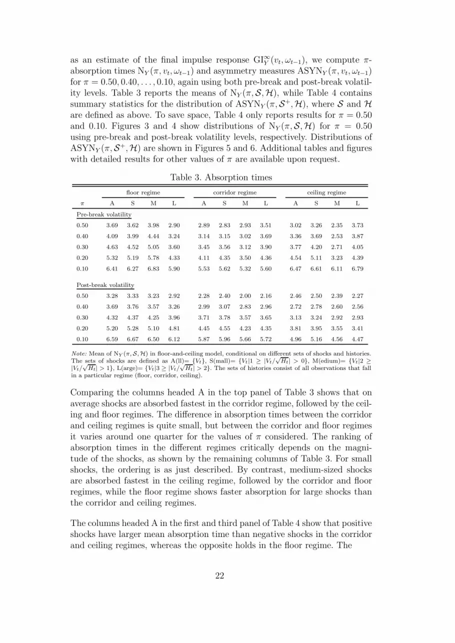
as an estimate of the final impulse response GI∞Y (vt, ωt−1), we compute π-absorption times NY (π, vt, ωt−1) and asymmetry measures ASYNY (π, vt, ωt−1)for π = 0.50, 0.40, . . . , 0.10, again using both pre-break and post-break volatil-ity levels. Table 3 reports the means of NY (π,S,H), while Table 4 containssummary statistics for the distribution of ASYNY (π,S+,H), where S and Hare defined as above. To save space, Table 4 only reports results for π = 0.50and 0.10. Figures 3 and 4 show distributions of NY (π,S,H) for π = 0.50using pre-break and post-break volatility levels, respectively. Distributions ofASYNY (π,S+,H) are shown in Figures 5 and 6. Additional tables and figureswith detailed results for other values of π are available upon request.

Table 3. Absorption times

floor regime corridor regime ceiling regime

π A S M L A S M L A S M L

Pre-break volatility

0.50 3.69 3.62 3.98 2.90 2.89 2.83 2.93 3.51 3.02 3.26 2.35 3.73

0.40 4.09 3.99 4.44 3.24 3.14 3.15 3.02 3.69 3.36 3.69 2.53 3.87

0.30 4.63 4.52 5.05 3.60 3.45 3.56 3.12 3.90 3.77 4.20 2.71 4.05

0.20 5.32 5.19 5.78 4.33 4.11 4.35 3.50 4.36 4.54 5.11 3.23 4.39

0.10 6.41 6.27 6.83 5.90 5.53 5.62 5.32 5.60 6.47 6.61 6.11 6.79

Post-break volatility

0.50 3.28 3.33 3.23 2.92 2.28 2.40 2.00 2.16 2.46 2.50 2.39 2.27

0.40 3.69 3.76 3.57 3.26 2.99 3.07 2.83 2.96 2.72 2.78 2.60 2.56

0.30 4.32 4.37 4.25 3.96 3.71 3.78 3.57 3.65 3.13 3.24 2.92 2.93

0.20 5.20 5.28 5.10 4.81 4.45 4.55 4.23 4.35 3.81 3.95 3.55 3.41

0.10 6.59 6.67 6.50 6.12 5.87 5.96 5.66 5.72 4.96 5.16 4.56 4.47

Note: Mean of NY (π,S,H) in floor-and-ceiling model, conditional on different sets of shocks and histories.The sets of shocks are defined as A(ll)= Vt, S(mall)= Vt|1 ≥ |Vt/

√Ht| > 0, M(edium)= Vt|2 ≥

|Vt/√

Ht| > 1, L(arge)= Vt|3 ≥ |Vt/√

Ht| > 2. The sets of histories consist of all observations that fallin a particular regime (floor, corridor, ceiling).

Comparing the columns headed A in the top panel of Table 3 shows that onaverage shocks are absorbed fastest in the corridor regime, followed by the ceil-ing and floor regimes. The difference in absorption times between the corridorand ceiling regimes is quite small, but between the corridor and floor regimesit varies around one quarter for the values of π considered. The ranking ofabsorption times in the different regimes critically depends on the magni-tude of the shocks, as shown by the remaining columns of Table 3. For smallshocks, the ordering is as just described. By contrast, medium-sized shocksare absorbed fastest in the ceiling regime, followed by the corridor and floorregimes, while the floor regime shows faster absorption for large shocks thanthe corridor and ceiling regimes.

The columns headed A in the first and third panel of Table 4 show that positiveshocks have larger mean absorption time than negative shocks in the corridorand ceiling regimes, whereas the opposite holds in the floor regime. The

22

Table 4. Asymmetry measures for absorption times

floor regime corridor regime ceiling regime

A S M L A S M L A S M L

π = 0.50, pre-break volatility

Mean −0.12 −0.20 0.17 −0.74∗ 0.31 1.49∗ −1.88∗ −3.02∗ 0.06 0.62 −0.64 −3.52∗

St.dev. 2.52 2.47 2.73 1.68 2.95 2.47 2.45 1.40 2.93 3.02 2.13 2.46

Skewness −0.68 −0.89 −0.52 1.70 0.05 0.87 −1.32 −2.82 −0.33 −0.21 −2.19 −0.94

SAMα∗ 1.00 1.00 1.00 0.38 1.00 0.84 0.82 0.02 1.00 0.84 0.96 0.23

EQIα∗ 1.00 1.00 1.00 0.36 1.00 1.00 1.00 0.01 1.00 1.00 1.00 0.35

HDRα∗ 1.00 1.00 1.00 0.11 1.00 1.00 1.00 0.01 1.00 1.00 1.00 0.38

π = 0.50, post-break volatility

Mean −0.33 0.00 −0.96 −1.07∗ −0.16 −0.22 −0.01 −0.31 −0.31 −0.05 −0.83∗ −0.71

St.dev. 2.43 2.44 2.38 1.67 1.29 1.54 0.21 1.18 2.04 2.14 1.72 1.67

Skewness −0.10 0.00 −0.46 −0.32 −4.27 −3.48 −19.01 −5.01 −0.59 −0.50 −1.34 −2.62

SAMα∗ 1.00 1.00 0.90 0.41 1.00 1.00 1.00 1.00 1.00 1.00 0.90 0.97

EQIα∗ 1.00 1.00 1.00 0.65 1.00 1.00 1.00 1.00 1.00 1.00 1.00 1.00

HDRα∗ 1.00 1.00 1.00 0.67 1.00 1.00 1.00 1.00 1.00 1.00 1.00 1.00

π = 0.10, pre-break volatility

Mean −0.33 −1.00 1.05∗ 0.56 1.98∗ 3.40∗ −0.47 −3.16∗ 0.79 1.46 −0.15 −2.85∗

St.dev. 3.02 3.11 2.39 1.96 3.45 2.22 3.79 2.05 3.13 3.24 2.16 2.64

Skewness −0.88 −1.04 0.37 −0.43 −1.05 0.38 −1.10 −1.32 0.15 0.25 −1.47 −1.25

SAMα∗ 1.00 0.75 0.41 0.80 0.65 0.10 1.00 0.12 0.78 0.65 1.00 0.33

EQIα∗ 1.00 0.85 0.63 0.95 0.52 0.11 1.00 0.12 0.94 0.66 1.00 0.20

HDRα∗ 0.60 0.59 0.58 1.00 0.50 0.11 0.70 0.18 1.00 0.74 1.00 0.34

π = 0.10, post-break volatility

Mean −0.41 0.12 −1.46∗ −1.47∗ 0.00 0.19 −0.28∗ −1.02∗ −0.70 −0.02 −1.98∗ −2.57∗

St.dev. 2.93 2.82 2.96 2.09 1.73 2.03 0.56 1.26 2.94 2.87 2.63 2.10

Skewness −0.18 −0.14 −0.28 0.34 −2.01 −2.04 −2.08 −2.17 −0.30 −0.14 −1.21 −1.97

SAMα∗ 1.00 1.00 0.84 0.55 1.00 1.00 1.00 0.51 0.83 1.00 0.54 0.16

EQIα∗ 1.00 1.00 0.99 0.52 1.00 1.00 1.00 0.86 1.00 1.00 0.62 0.15

HDRα∗ 1.00 1.00 1.00 0.15 1.00 1.00 1.00 1.00 1.00 1.00 0.73 0.28

Note: Summary statistics for asymmetry measure ASYNY (π,S+,H) in floor-and-ceiling model. The dif-ferent sets of shocks are defined as A(ll)= Vt, S(mall)= Vt|1 ≥ |Vt/

√Ht| > 0, M(edium)= Vt|2 ≥

|Vt/√

Ht| > 1, L(arge)= Vt|3 ≥ |Vt/√

Ht| > 2. The sets of histories consist of all observations that fall ina particular regime (floor, corridor, ceiling). Entries in rows labelled Mean which are larger than two timesσASYNY (π,S+,H)/

√nS are marked with an asterisk, where σASYNY (π,S+,H) is the standard deviation of

ASYNY (π,S+,H) and nS is the number of shocks vt for which ASYNY (π, vt, ωt−1) is computed. Entriesin rows labelled Zα∗ represent the minimum value of α ∈ (0, 1) such that 0 would not be included in therelevant confidence region Zα, Z = SAM , EQI and HDR.

average asymmetry is not significantly different from zero though. Turning tothe subsets of shocks of different magnitudes, we observe interesting differencesin the absorption time for π = 0.50 or, put differently, the half-life of shocks.In the floor and ceiling regimes, positive large shocks are absorbed faster thannegative large shocks, while there is no significant asymmetry for small and

23

(a) A, floor (b) A, corridor (c) A, ceiling

(d) N, floor (e) N, corridor (f) N, ceiling

(g) P, floor (h) P, corridor (i) P, ceiling

Fig. 3. Distributions of absorption times in floor-and-ceiling model for π = 0.50using pre-break volatility, conditional on different sets of shocks and histories.The sets of shocks are defined as A(ll)= Vt, N(egative)= Vt|Vt < 0, andP(ositive)= Vt|Vt > 0. The sets of histories consist of all observations that fall ina particular regime (floor, corridor, ceiling).

medium shocks in these regimes based on the standard error σASYNY (π,S+,H)/√

nS .In the corridor regime, large positive shocks have a shorter half-life as well,but in addition the same holds for medium-sized shocks. By contrast, smallpositive shocks in the corridor regime have a longer half-life than negativeones. Similar patterns emerge for π = 0.10 in the third panel of Table 4. Alsonote that in the floor regime there is a ‘reversal’, in the sense that positivelarge shocks are absorbed faster for larger values of π, while they are absorbedslower for smaller values of π.

24

(a) A, floor (b) A, corridor (c) A, ceiling

(d) N, floor (e) N, corridor (f) N, ceiling

(g) P, floor (h) P, corridor (i) P, ceiling

Fig. 4. Distributions of absorption times in floor-and-ceiling model for π = 0.50using post-break volatility, conditional on different sets of shocks and histories.The sets of shocks are defined as A(ll)= Vt, N(egative)= Vt|Vt < 0, andP(ositive)= Vt|Vt > 0. The sets of histories consist of all observations that fall ina particular regime (floor, corridor, ceiling).

Comparing the two panels of Table 3 reveals that the decline in volatilityin 1984 has substantially reduced the average absorption times for shocksoccurring in the ceiling regime for all values of π considered. Interestingly,for the floor and corridor regimes we observe that the half-life of shocks hasbecome smaller, but that absorption times have become longer for smallervalues of π, although the latter changes are fairly small. The volatility changehas also had mixed effects on the asymmetry properties of NY (π,S,H), whichcan be learned from Table 4. Asymmetry has been hardly affected for certain

25

(a) S, floor (b) S, corridor (c) S, ceiling

(d) M, floor (e) M, corridor (f) M, ceiling

(g) L, floor (h) L, corridor (i) L, ceiling

Fig. 5. Distributions of asymmetry measures for absorption times in floor-and-ceilingmodel for π = 0.50 using pre-break volatility, conditional on different sets of shocksand histories. The sets of shocks are defined as S(mall)= Vt|1 ≥ |Vt/

√Ht| > 0,

M(edium)= Vt|2 ≥ |Vt/√

Ht| > 1, L(arge)= Vt|3 ≥ |Vt/√

Ht| > 2. The sets ofhistories consist of all observations that fall in a particular regime (floor, corridor,ceiling).

subsets of shocks S and histories H and for certain values of π, such as largeshocks occurring in the floor regime for π = 0.50 or occurring in the ceilingregime for π = 0.10. In other cases, asymmetry has disappeared, see thehalf-life of large shocks occurring in the ceiling regime or small shocks in thecorridor regime for both π = 0.50 and 0.10. The half-life of medium shocks inthe corridor regime provides the most striking example. As can be seen frompanel (e) of Figures 5 and 6 the distribution of ASYNY (π,S,H) has effectivelycollapsed to a spike at 0 in this case. In still other cases, asymmetry has been

26

(a) S, floor (b) S, corridor (c) S, ceiling

(d) M, floor (e) M, corridor (f) M, ceiling

(g) L, floor (h) L, corridor (i) L, ceiling

Fig. 6. Distributions of asymmetry measures for absorption times in floor-and–ceiling model for π = 0.50 using post-break volatility, conditional on differ-ent sets of shocks and histories. The sets of shocks are defined as A(ll)= Vt,S(mall)= Vt|1 ≥ |Vt/

√Ht| > 0, M(edium)= Vt|2 ≥ |Vt/

√Ht| > 1,

L(arge)= Vt|3 ≥ |Vt/√

Ht| > 2. The sets of histories consist of all observationsthat fall in a particular regime (floor, corridor, ceiling).

introduced, see large shocks in the floor regime and medium shocks in theceiling regime at π = 0.10. Panels (d) and (f) of Figures 5 suggest that theabsorption of medium-sized shocks in the floor and ceiling regimes also hasbecome more asymmetric, but according to Table 4 this is not significant.

Finally, we note that our empirical analysis in this Section is based entirelyon a univariate reduced-form model. This does not allow us to distinguishbetween different possible sources or explanations for the observed asymme-

27

tries in absorption times and changes therein. We therefore restrict ourselvesto documenting their existence. Investigating the underlying causes requires astructural modeling approach, and is left for future research.

6 Concluding remarks

In this paper we proposed a new tool that can be used to examine the prop-erties of univariate and multivariate nonlinear time series models. This tool,which we called the absorption rate, can be viewed as complementary to thefamiliar impulse response function, as both consider different aspects of thepropagation of shocks. The absorption rate can be used to examine whetherthe propagation of different types of shocks, such as large and small shocks,positive and negative shocks, and shocks in various regimes, follows a differentpattern. In multivariate models, the absorption rate can also reveal whethershocks have longer lasting effects on certain variables than on others. Hence,the absorption rate can help to interpret a possibly complicated nonlinearmodel, with potentially a large number of parameters.

In a sense, the absorption rate is informative for the degree of nonlinearity aparticular model is picking up from the data. If all kinds of shocks have similareffects on the future path of a time series variable, the nonlinear model canbe said to have linear properties, even though parameters for the nonlinearcomponent are highly significant. Such a finding can imply that either there isnot enough nonlinearity in the data or the model is not capturing the nonlinearfeatures adequately.

The above leads to the suggestion that the absorption rate can provide usefulprior information as to how successful a particular nonlinear model will bewhen it comes to out-of-sample forecasting. With respect to our empiricalapplication to US GDP, we found considerable evidence for asymmetry in theabsorption rate of different types of shocks in the different regimes in thefloor-and-ceiling model. However, it appears that asymmetry became muchless pronounced due to a large decline in output volatility in the 1980s. Hence,it may not come as a surprise that linear models tend to beat this nonlinearmodel in terms of forecasting output growth during recent years.

Acknowledgements

Helpful discussions with Clive Granger and Simon Potter are gratefully ac-knowledged, as well as useful comments and suggestions from an associate ed-itor and an anonymous referee. The first draft of this paper (which circulated

28

under the title ‘Common persistence in nonlinear autoregressive models’) waswritten while the third author was enjoying the hospitality of the Departmentof Economics of the University of California, San Diego.

References

Altissimo, F., Violante, G.L., 2001. The non-linear dynamics of output and unem-ployment in the US. J. Appl. Econometrics 16, 461–481.

Atanasova, C., 2003. Credit market imperfections and business cycle dynamics: Anonlinear approach. Stud. Nonl. Dyn. Econometrics 7(4), article 5.

Balke, N.S., 2000. Credit and economic activity: Credit regimes and nonlinear prop-agation of shocks. Rev. Econom. Stat. 82, 344–349.

Balke, N.S., Brown, S.P.A., Yucel, M.K., 2002. Oil price shocks and the US economy:Where does the asymmetry originate?. Energy J. 23, 27–52.

Beaudry, P., Koop, G., 1993. Do recessions permanently change output?. J. Mon.Econom. 31, 149–163.

Camacho, M., 2005. Markov-switching stochastic trends and economic fluctuations.J. Econom. Dyn. Control 29, 135–158.

Chan, K.S., Tong, H., 1986. On estimating thresholds in autoregressive models. J.Time Series Anal. 7, 178–190.

Chan, K.S., Tong, H., 2004. Testing for multimodality with dependent data. Biometrika91, 113–123.

Chen, S.L., Tsai, L.J., Wu, J.L., 2004. A revisit to liquidity effects - Evidence froma nonlinear approach. J. Macroeconom. 26, 501–517.

Clements, M.P., Krolzig, H.-M., 2002. Can oil shocks explain asymmetries in theUS business cycle?. Emp. Econom. 27, 185–204.

Dufour, A., Engle, R.F., 2000. Time and the price impact of a trade. J. Finance 55,2467–2498.

Dufrenot, G., Mignon, V., Peguin-Feissolle, A., 2004. Business cycle asymmetry andmonetary policy: a further investigation using MRSTAR models. Econom. Mod.21, 37–71.

Fan, J., Yao, Q., Tong, H., 1996. Estimation of conditional densities and sensitivitymeasures in nonlinear dynamical systems. Biometrika 83, 189–206.

Franses, P.H., van Dijk, D., 2000. Nonlinear Time Series Models in Empirical Fi-nance, Cambridge University Press, Cambridge.

Galbraith, J.W., 2003. Content horizons for univariate time series forecasts. Inter-nat. J. Forecasting 19, 43–55.

Gallant, A.R., Rossi, P.E., Tauchen, G., 1993. Nonlinear dynamic structures. Econo-metrica 61, 871–908.

Granger, C.W.J., Terasvirta, T., 1993. Modelling Nonlinear Economic Relation-ships, Oxford University Press, Oxford.

Grier, K.B., Henry, O.T., Olekalns, N., Shields, K., 2004. The asymmetric effects ofuncertainty on inflation and output growth. J. Appl. Econometrics 19, 551–565.

Hamilton, J.D., 1989. A new approach to the economic analysis of nonstationarytime series subject to changes in regime. Econometrica 57, 357–384.

Hyndman, R.J., 1995. Highest-density forecast regions for non-linear and non-normal

29

time series. J. Forecasting 14, 431–441.Kim, C.-J., Morley J., Piger, J., 2005. Nonlinearity and the permanent effects of

recessions. J. Appl. Econometrics 20, 291–309.Koop, G., 1996. Parameter uncertainty and impulse response analysis. J. Econo-

metrics 72, 135–149.Koop, G., Pesaran, M.H., Potter, S.M., 1996. Impulse response analysis in nonlinear

multivariate models. J. Econometrics 74, 119–147.Kuan, C.-M., White, H., 1994. Artificial neural networks: an econometric perspective

(with discussion). Econometric Rev. 13, 1–143.Lee, K.C., Pesaran, M.H., 1993. Persistence profiles and business cycle fluctuations

in a disaggregated model of UK output growth. Richerche Economiche 47, 293–322.

Lutkepohl, H., 2005. New Introduction to Multiple Time Series Analysis, Springer-Verlag, Berlin.

McConnell, M.M., Perez-Quiros, G., 2000. Output fluctuations in the United States:What has changed since the early 1980s?. Amer. Econom. Review 90, 1464–1476.

Pesaran, M.H., Potter, S.M., 1997. A floor and ceiling model of US output. J.Econom. Dyn. Control 21, 661–695.

Pesaran, M.H., Shin, Y., 1996. Cointegration and speed of convergence to equilib-rium. J. Econometrics 71, 117–143.

Pesaran, M.H., Shin, Y., 1998. Generalized impulse response analysis in linear mul-tivariate models. Econom. Letters 58, 17–29.

Potter, S.M., 1994. Asymmetric economic propagation mechanisms. In: W. Semm-ler (Ed.), Business Cycles: Theory and Empirical Methods, Kluwer AcademicPublishers, Boston, 313–330.

Potter, S.M., 1995a. Nonlinear models of economic fluctuations. In: K. Hoover (Ed.),Macroeconometrics - Developments, Tensions and Prospects, Kluwer, Boston,517–560.

Potter, S.M., 1995b. A nonlinear approach to US GNP. J. Appl. Econometrics 10,109–125.

Potter, S.M., 2000. Nonlinear impulse response functions. J. Econom. Dyn. Control24, 1425–1446.

Sensier, M., van Dijk, D., 2004. Testing for volatility changes in US macroeconomictime series. Rev. Econom. Stat. 86, 833–839.

Skalin, J., Terasvirta, T., 2002. Modeling asymmetries and moving equilibria inunemployment rates. Macroeconom. Dyn. 6, 202–241.

Stock, J.H., Watson, M.W., 2003. Has the business cycle changed? Evidence andexplanations. In: Monetary Policy and Uncertainty: Adapting to Changing Econ-omy symposium proceedings, Federal Reserve Bank of Kansas City, 9–56.

Taylor, M.P., Peel, D.A., 2000. Nonlinear adjustment, long-run equilibrium andexchange rate fundamentals. J. Internat. Money Fin. 19, 33–53.

Taylor, M.P., Peel D.A., Sarno, L., 2001. Nonlinear mean-reversion in exchangerate rates: towards a solution to the purchasing power parity puzzles. Internat.Econom. Rev. 42, 1015–1042.

Terasvirta, T., 1994. Specification, estimation, and evaluation of smooth transitionautoregressive models. J. Amer. Stat. Ass. 89, 208–218.

Terasvirta, T., 1995. Modelling nonlinearity in US gross national product 1889-1987.

30

Emp. Econom. 20, 577–598.Tong, H., 1990. Non-Linear Time Series: a Dynamical Systems Approach, Oxford

University Press, Oxford.van Dijk, D., Terasvirta, T., Franses, P.H., 2002. Smooth transition autoregressive

models - a survey of recent developments. Econometric Rev. 21, 1–47.Weise, C.L., 1999. The asymmetric effects of monetary policy: A nonlinear vector

autoregression approach. J. Money Credit Banking 31, 85–108.Yao, Q., Tong, H., 1994. Quantifying the influence of initial values on non-linear

prediction. J. Royal Stat. Soc. B 56, 701–725.

31