Flow Coefficient Definition

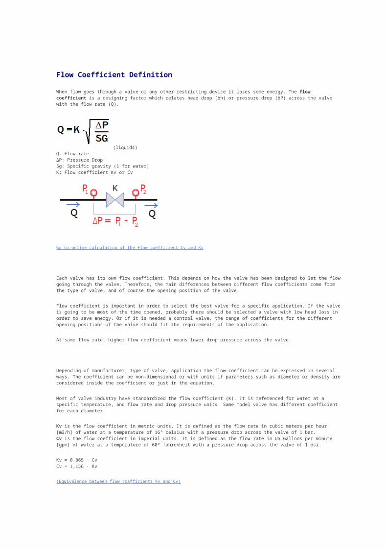
When flow goes through a valve or any other restricting device it loses some energy. The flow coefficient is a designing factor which relates head drop (Δh) or pressure drop (ΔP) across the valve with the flow rate (Q).

(liquids) Q: Flow rateΔP: Pressure DropSg: Specific gravity (1 for water)K: Flow coefficient Kv or Cv

Go to online calculation of the Flow coefficient Cv and Kv

Each valve has its own flow coefficient. This depends on how the valve has been designed to let the flowgoing through the valve. Therefore, the main differences between different flow coefficients come from the type of valve, and of course the opening position of the valve.

Flow coefficient is important in order to select the best valve for a specific application. If the valveis going to be most of the time opened, probably there should be selected a valve with low head loss in order to save energy. Or if it is needed a control valve, the range of coefficients for the different opening positions of the valve should fit the requirements of the application.

At same flow rate, higher flow coefficient means lower drop pressure across the valve.

Depending of manufacturer, type of valve, application the flow coefficient can be expressed in several ways. The coefficient can be non-dimensional or with units if parameters such as diameter or density areconsidered inside the coefficient or just in the equation.

Most of valve industry have standardized the flow coefficient (K). It is referenced for water at a specific temperature, and flow rate and drop pressure units. Same model valve has different coefficient for each diameter.

Kv is the flow coefficient in metric units. It is defined as the flow rate in cubic meters per hour [m3/h] of water at a temperature of 16º celsius with a pressure drop across the valve of 1 bar.Cv is the flow coefficient in imperial units. It is defined as the flow rate in US Gallons per minute [gpm] of water at a temperature of 60º fahrenheit with a pressure drop across the valve of 1 psi.

Kv = 0.865 · CvCv = 1,156 · Kv

(Equivalence between flow coefficients Kv and Cv)

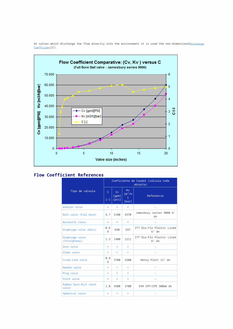
At valves which discharge the flow directly into the environment it is used the non-dimensionalDischargeCoefficient(C).

Flow Coefficient References

Tipo de válvula

Coeficiente de Caudal (válvula todaabierta)

C

[-]

Cv[gpm][psi]

Kv[m³/h]

[bar]

Referencia

Annular valve ÷ ÷ ÷ -

Ball valve (Full bore) 4.7 5100 4370 Jamesbury series 9000 6"dn

Butterlfy valve ÷ ÷ ÷ -

Diaphragm valve (Weir) 0.64 690 597 ITT Dia-Flo Plastic Lined

6" dn

Diaphragm valve (Straightway) 1.3 1400 1211 ITT Dia-Flo Plastic Lined

6" dn

Gate valve ÷ ÷ ÷ -

Globe valve ÷ ÷ ÷ -

Fixed Cone valve 0.86 3700 3200 Henry Platt 12" dn

Needle valve ÷ ÷ ÷ -

Plug valve ÷ ÷ ÷ -

Pinch valve ÷ ÷ ÷ -Rubber Duck-Bill check valve 1.0 4300 3700 EVR CPF/CPO 300mm dn

Spherical valve ÷ ÷ ÷ -

Tilting disc check valve 0.93 1160 1003 Val-matic 6" dn

(*) Water density reference (1000kg/m3) to calculate C and Cv KV equivalencies

The flow coefficient of a device is a relative measure of its efficiency at allowing fluid flow. It describes the relationship between the pressure drop across an orifice, valve or other assembly and the corresponding flow rate.

Mathematically the flow coefficient can be expressed as:

where:Cv = Flow coefficient or flow capacity rating of valve.F = Rate of flow (US gallons per minute).SG = Specific gravity of fluid (Water = 1).ΔP = Pressure drop across valve (psi).

In more practical terms, the flow coefficient Cv is the volume (in US gallons) of water at 60°F that will flow per minute through a valve with a pressure drop of 1 psi across the valve.

The use of the flow coefficient offers a standard method of comparing valve capacities and sizing valves for specific applications that is widely accepted by industry. The general definition of the flow coefficient can be expanded into equations modeling the flow of liquids, gases and steam as follows:

Coefficient of discharge is the ratio of actual flow rate to theoretical discharge.

For gas flow in a pneumatic system the Cv for the same assembly can be used with a more complex equation.[1][2] Absolute pressures (psia) must be used for gas rather than simply differential pressure.

For air flow at room temperature, when the outlet pressure is less than 1/2 the absolute inlet pressure, the flow becomes quite simple (although it reaches sonic velocity internally). With Cv = 1.0 and 200 psia inlet pressure the flow is 100 standard cubic feet per minute (scfm). The flow is proportional to the absolute inlet pressure so that the flowin scfm would equal the Cv flow coefficient if the inlet pressure were reduced to 2 psia and the outlet were connected to a vacuum with less than 1 psi absolute pressure (1.0 scfm when Cv = 1.0, 2 psia input).

Using the Flow Coefficient (Cv) to Characterize the Performance of a Piping System

Fluid flow through a piping system that consists of components such asvalves, fittings, heat exchangers, nozzles, filters, and pipelines willresult in a loss of energy due to the friction between the fluid andinternal surfaces, changes in the direction of the flow path,obstructions in the flow path, and changes in the cross-section andshape of the flow path.

The energy loss, or head loss, will be seen as a pressure drop acrossthe piping system and each component in the system. There are differentways to characterize the impact of these factors with regard to the flowrate through the component and the resulting pressure drop.

One way is to characterize the amount of resistance that is offered by thesystem or components. The resistance can be given a numerical value as aresistance coefficient (K) or by the pipe length (or equivalent length),which can be used in the 2nd order Darcy equation to calculate the amountof head loss:

Where: HL = head loss (ft)f = Darcy friction factor (unitless)Leqv = pipe length (ft)D = pipe internal diameter (ft)v = fluid velocity (ft/sec)g = gravitational constant (ft/sec2)K= resistance coefficient (unitless)

The pressure drop resulting from the head loss is given by:

Where: dP = pressure drop (psi)rho = fluid density (lb/ft3)

The resistance of a piping system is constant when all the valves(including control valves) remain in one position. When the position ofa valve is changed, the resistance of the valve and therefore the entiresystem is changed. The change in resistance results in a change of flowrate and pressure drop in the system. Conversely, if the resistanceremains constant and the differential pressure changes, the effect onthe flow rate can be calculated.

Another way to characterize the performance of the system or a componentis by its capacity. The capacity can be expressed with a numerical valueas a flow coefficient (CV) that equates the amount of pressure drop tothe flow rate by the following equation:

Where: Cv = flow coefficient (unitless)Q = flow rate (gpm)SG = fluid specific gravity

The flow coefficient is commonly used by control valve manufacturers tocharacterize the performance of their valves with a change in valveposition. Nozzle and sprinkler manufacturers also use the flowcoefficient, except that they generally refer to it as a dischargecoefficient. For a nozzle or sprinkler, when the inlet pressure changes,the flow rate through the nozzle will change proportionally, as given bythe CV equation above and holding CV constant.

Just as with the system resistance, the system capacity remains constantas long as the positions of the valves in the system are constant. Aconstant flow coefficient allows for calculating the flow rate when thedifferential pressure changes.

This concept can be used to simplify piping systems for analysis usingEngineered Software's PIPE-FLO or Flow of Fluids programs. If thepressure (or differential pressure) and flow rate at a point in thesystem is known and the system resistance downstream from this point isconstant, the downstream system can be simplified and represented with aflow coefficient, CV.

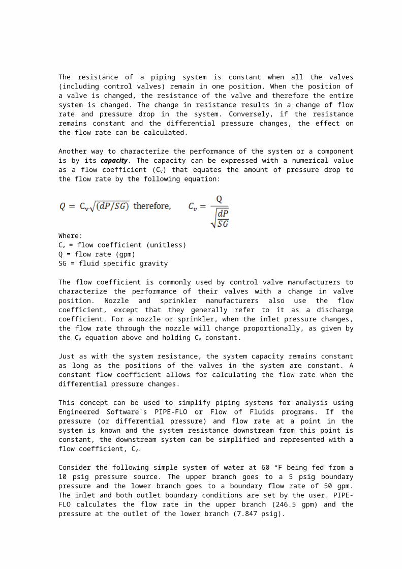
Consider the following simple system of water at 60 °F being fed from a10 psig pressure source. The upper branch goes to a 5 psig boundarypressure and the lower branch goes to a boundary flow rate of 50 gpm.The inlet and both outlet boundary conditions are set by the user. PIPE-FLO calculates the flow rate in the upper branch (246.5 gpm) and thepressure at the outlet of the lower branch (7.847 psig).

To determine what happens to the flow rate and pressure in the upperbranch when the flow rate in the lower branch changes, assuming theconfiguration of the upper branch remains the same (i.e. valve positionsin the upper branch are not changed), the system should be modified toobtain an equivalent system, as shown below. A short length of pipe(0.0001 ft) is added to the upper branch at the outlet with a boundarypressure of 0 psig and a fixed CV fitting installed in the pipe. TheCV is calculated using the CV formula above, using SG=1.0 (for water at60 °F), the calculated flow rate, and a differential pressure of 5 psid.

The calculated model confirms that the two systems are equivalent sincethe calculated flow rate in the upper branch is 246.5 gpm and thecalculated pressure at the node is 5 psig.

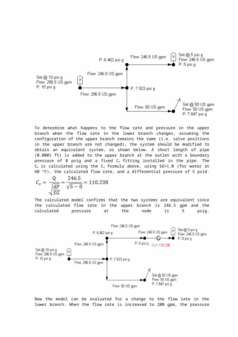
Now the model can be evaluated for a change to the flow rate in thelower branch. When the flow rate is increased to 200 gpm, the pressure

at the common junction decreased from 7.923 psig to 6.049 psig. Thisresults in a lower differential pressure in the upper branch andtherefore a lower flow rate in the upper branch. The flow rate in theupper branch goes from 246.5 to 214.8 gpm, and the pressure at theoutlet goes from 5 psig to 3.797 psig.

This method of simplifying a system can be used when the flow rate andpressure are known at a given point in the system and it is known thatthe system downstream of that point remains constant with regard tovalve positions. It can also be used when the differential pressure isknown for a given flow rate and the components within the boundariesthat define the differential pressure remain constant.

This method can also be used for evaluating the performance of a closedloop system. Consider the following system with three heat exchangers,each with a flow rate of about 200 gpm. The flow control valves aremanually operated valves and have Cv data entered for the range of valvepositions (each valve has different Cv values so they are notidentical). The three heat exchangers have identical head loss curves.This is a common configuration for a plant with heat exchangers locatedthroughout the facility.

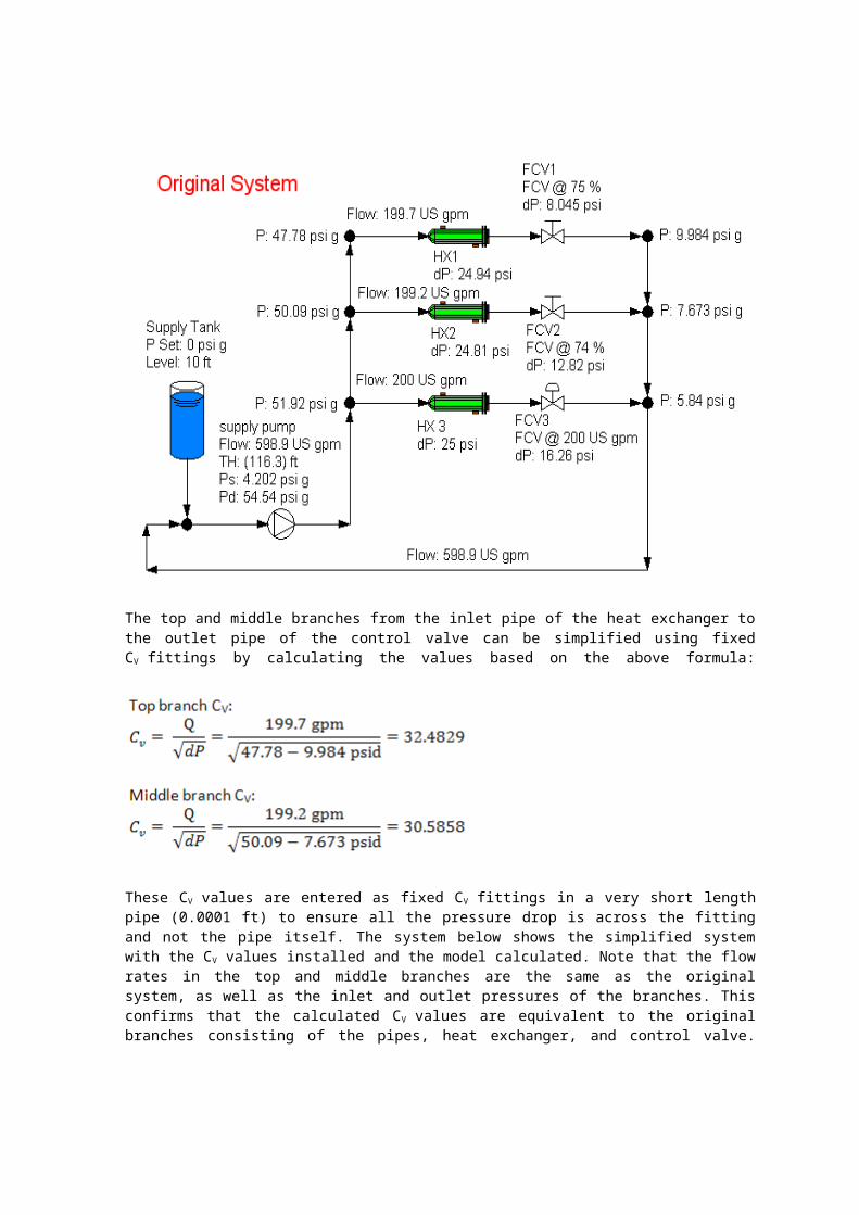
The top and middle branches from the inlet pipe of the heat exchanger tothe outlet pipe of the control valve can be simplified using fixedCV fittings by calculating the values based on the above formula:

These CV values are entered as fixed CV fittings in a very short lengthpipe (0.0001 ft) to ensure all the pressure drop is across the fittingand not the pipe itself. The system below shows the simplified systemwith the CV values installed and the model calculated. Note that the flowrates in the top and middle branches are the same as the originalsystem, as well as the inlet and outlet pressures of the branches. Thisconfirms that the calculated CV values are equivalent to the originalbranches consisting of the pipes, heat exchanger, and control valve.

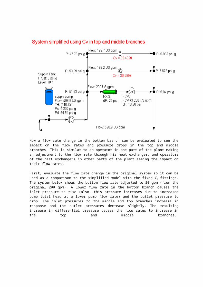
Now a flow rate change in the bottom branch can be evaluated to see theimpact on the flow rates and pressure drops in the top and middlebranches. This is similar to an operator in one part of the plant makingan adjustment to the flow rate through his heat exchanger, and operatorsof the heat exchangers in other parts of the plant seeing the impact ontheir flow rates.

First, evaluate the flow rate change in the original system so it can beused as a comparison to the simplified model with the fixed CV fittings.The system below shows the bottom flow rate adjusted to 50 gpm (from theoriginal 200 gpm). A lower flow rate in the bottom branch causes theinlet pressure to rise (also, this pressure increases due to increasedpump total head at a lower pump flow rate) and the outlet pressure todrop. The inlet pressures to the middle and top branches increase inresponse and the outlet pressures decrease slightly. The resultingincrease in differential pressure causes the flow rates to increase inthe top and middle branches. 

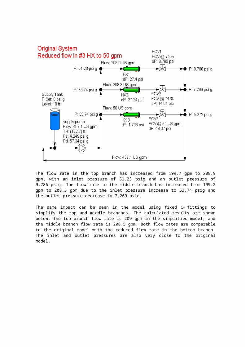
The flow rate in the top branch has increased from 199.7 gpm to 208.9gpm, with an inlet pressure of 51.23 psig and an outlet pressure of9.786 psig. The flow rate in the middle branch has increased from 199.2gpm to 208.3 gpm due to the inlet pressure increase to 53.74 psig andthe outlet pressure decrease to 7.269 psig.

The same impact can be seen in the model using fixed CV fittings tosimplify the top and middle branches. The calculated results are shownbelow. The top branch flow rate is 209 gpm in the simplified model, andthe middle branch flow rate is 208.5 gpm. Both flow rates are comparableto the original model with the reduced flow rate in the bottom branch.The inlet and outlet pressures are also very close to the originalmodel. 

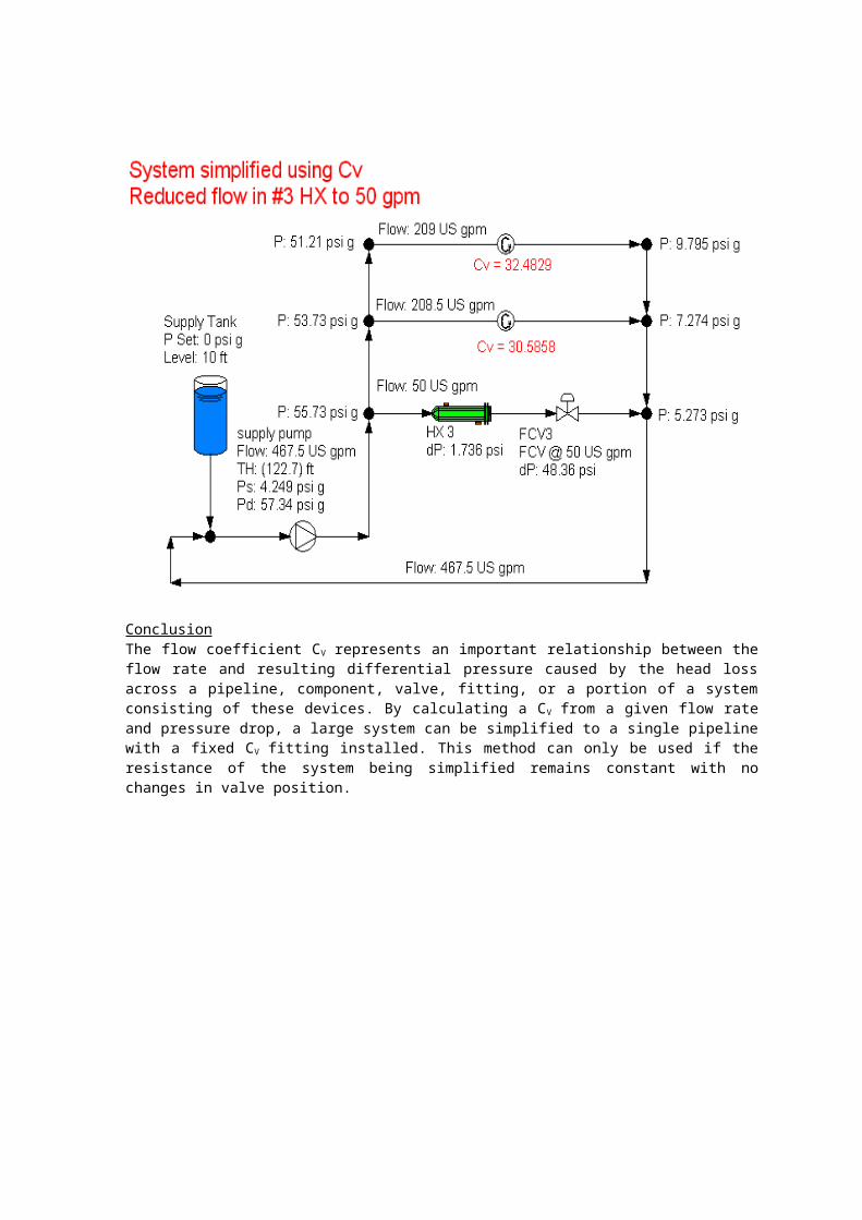
ConclusionThe flow coefficient CV represents an important relationship between theflow rate and resulting differential pressure caused by the head lossacross a pipeline, component, valve, fitting, or a portion of a systemconsisting of these devices. By calculating a CV from a given flow rateand pressure drop, a large system can be simplified to a single pipelinewith a fixed CV fitting installed. This method can only be used if theresistance of the system being simplified remains constant with nochanges in valve position.

Pressure Drop in Pipe Fittings and ValvesA Discussion of the Equivalent Length (Le/D), ResistanceCoefficient (K) and Valve Flow Coefficient (Cv) Methods

Copyright © Harvey Wilson - Katmar SoftwareOctober 2012

If you are looking for a calculator to perform pipe sizing and pressure drop calculations please jump tothe AioFlo page.

1. Introduction

The sizing of pipes for optimum economy requires that engineers be able to accurately calculate the flowrates and pressure drops in those pipes. The purpose of this document is to discuss the various methodsavailable to support these calculations. The focus will be on the methods for calculating the minorlosses in pipe sizing and to consider in particular the following aspects:

the advantages and disadvantages of each method

Reynolds Number and the flow regime (turbulent vs laminar)

the fitting size

the roughness of the fitting

the roughness of the attached piping

converting data from one method to another

2. Background

Over the years excellent progress has been made in developing methods for determining the pressure dropwhen fluids flow through straight pipes. Accurate pipe sizing procedures are essential to achieve aneconomic optimum by balancing capital and running costs. Industry has converged on the Darcy-Weisbachmethod, which is remarkably simple considering the scope of applications that it covers.The Darcy-Weisbach formula is usually used in the following form:

Equation (1) expresses the pressure loss due to friction in the pipe as a head (hL) of the flowing fluid.

The terms and dimensions in Equation (1) are:hL =head of fluid, dimension is lengthƒ =Moody friction factor (also called Darcy-Weisbach friction factor), dimensionlessL =straight pipe, dimension is lengthD= inside diameter of pipe, dimension is lengthv =average fluid velocity (volumetric flow / cross sectional area), dimension is length/timeg=acceleration due to earth's gravity, dimension is length/time2

The dimensions in Equation (1) can be in any consistent set of units. If the Fanning friction factor isused instead of the Moody friction factor then ƒ must be replaced by 4ƒ.

In long pipelines most of the pressure drop is due to the friction in the straight pipe, and thepressure drop caused by the fittings and valves is termed the "minor loss". As pipes get shorter andmore complicated the proportion of the losses due to the fittings and valves gets larger, but byconvention are still called the "minor losses".Over the last few decades there have been considerable advances in the accurate determination of theminor losses, but as of now they cannot be determined with the same degree of accuracy as the majorlosses caused by friction in the straight pipe. This situation is aggravated by the fact that theserecent developments have not filtered through to all levels of engineering yet, and there are many olddocuments and texts still around that use older and less accurate methods. There is still considerableconfusion amongst engineers over which are the best methods to use and even how to use them.Unfortunately one of the most widely used and respected texts, which played a major role in advancingthe state of the art, has added to this confusion by including errors and badly worded descriptions.(See section 4 below)Nevertheless, by employing the currently available knowledge and exercising care the minor losses can bedetermined with more than sufficient accuracy in all but the most critical situations.

3. The Three Methods for Minor Loss Determination

The 3 methods which are used to calculate the minor losses in pipe sizing exercises are the equivalentlength (Le/D), the resistance coefficient (K) and the valve flow coefficient (Cv), although the Cv methodis almost exclusively used for valves. To further complicate matters, the resistance coefficient (K)method has several levels of refinement and when using this procedure it is important to understand howthe K value was determined and its range of applicability. There are also several definitions for Cv,and these are discussed below.For all pipe fittings it is found that the losses are close to being proportional to the second term inEquation (1). This term (v2/2g) is known as the "velocity head". Both the equivalent length (Le/D) andthe resistance coefficient (K) method are therefore aimed at finding the correct multiplier for thevelocity head term.

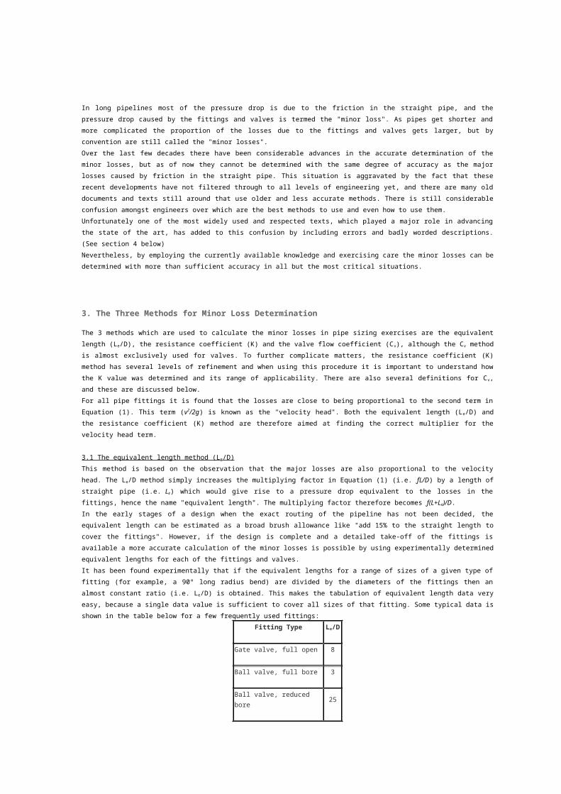
3.1 The equivalent length method (Le/D)This method is based on the observation that the major losses are also proportional to the velocityhead. The Le/D method simply increases the multiplying factor in Equation (1) (i.e. ƒL/D) by a length ofstraight pipe (i.e. Le) which would give rise to a pressure drop equivalent to the losses in thefittings, hence the name "equivalent length". The multiplying factor therefore becomes ƒ(L+Le)/D.In the early stages of a design when the exact routing of the pipeline has not been decided, theequivalent length can be estimated as a broad brush allowance like "add 15% to the straight length tocover the fittings". However, if the design is complete and a detailed take-off of the fittings isavailable a more accurate calculation of the minor losses is possible by using experimentally determinedequivalent lengths for each of the fittings and valves.It has been found experimentally that if the equivalent lengths for a range of sizes of a given type offitting (for example, a 90° long radius bend) are divided by the diameters of the fittings then analmost constant ratio (i.e. Le/D) is obtained. This makes the tabulation of equivalent length data veryeasy, because a single data value is sufficient to cover all sizes of that fitting. Some typical data isshown in the table below for a few frequently used fittings:

Fitting Type Le/D

Gate valve, full open 8

Ball valve, full bore 3

Ball valve, reduced bore 25

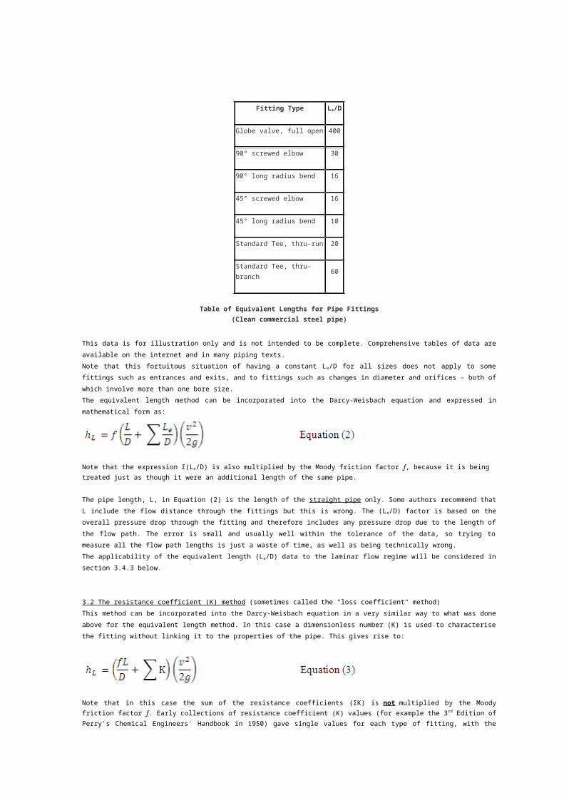
Fitting Type Le/D

Globe valve, full open 400

90° screwed elbow 30

90° long radius bend 16

45° screwed elbow 16

45° long radius bend 10

Standard Tee, thru-run 20

Standard Tee, thru-branch 60

Table of Equivalent Lengths for Pipe Fittings(Clean commercial steel pipe)

This data is for illustration only and is not intended to be complete. Comprehensive tables of data areavailable on the internet and in many piping texts.Note that this fortuitous situation of having a constant Le/D for all sizes does not apply to somefittings such as entrances and exits, and to fittings such as changes in diameter and orifices - both ofwhich involve more than one bore size.The equivalent length method can be incorporated into the Darcy-Weisbach equation and expressed inmathematical form as:

Note that the expression Σ(Le/D) is also multiplied by the Moody friction factor ƒ, because it is being treated just as though it were an additional length of the same pipe.

The pipe length, L, in Equation (2) is the length of the straight pipe only. Some authors recommend thatL include the flow distance through the fittings but this is wrong. The (Le/D) factor is based on theoverall pressure drop through the fitting and therefore includes any pressure drop due to the length ofthe flow path. The error is small and usually well within the tolerance of the data, so trying tomeasure all the flow path lengths is just a waste of time, as well as being technically wrong.The applicability of the equivalent length (Le/D) data to the laminar flow regime will be considered insection 3.4.3 below.

3.2 The resistance coefficient (K) method (sometimes called the "loss coefficient" method)This method can be incorporated into the Darcy-Weisbach equation in a very similar way to what was doneabove for the equivalent length method. In this case a dimensionless number (K) is used to characterisethe fitting without linking it to the properties of the pipe. This gives rise to:

Note that in this case the sum of the resistance coefficients (ΣK) is not multiplied by the Moodyfriction factor ƒ. Early collections of resistance coefficient (K) values (for example the 3rd Edition ofPerry's Chemical Engineers' Handbook in 1950) gave single values for each type of fitting, with the

intention that the value be applicable to all sizes of that fitting. As more research was done it wasfound that in general the resistance coefficient (K) decreased as the fitting size increased, and whenthe Hydraulic Institute published the "Pipe Friction Manual" in 1954 the coefficients were given in theform of graphs covering a wide range of sizes.

Up until that point in time the derived K values were for use in the fully turbulent flow regime only,and the 3rd Edition of Perry's Handbook makes specific mention of the non-applicability of the data tolaminar (or viscous) flow.The valve manufacturer, Crane Company, had been producing technical information for flow calculationssince 1935 and launched their Technical Paper No. 410 "Flow of Fluids through Valves, Fittings and Pipe"in 1942. Since then this document has been regularly updated and is probably the most widely used sourceof piping design data in the English speaking world. The 1976 edition of Crane TP 410 saw the watershedchange from advocating the equivalent length (Le/D) method to their own version of the resistancecoefficient (K) method. This is widely referred to in the literature as the "Crane 2 friction factor"method or simply the "Crane K" method. Crane provided data for an extensive range of fittings, andprovided a method for adjusting the K value for the fitting size. Unfortunately this welcome advanceintroduced a significant error and much confusion. The details of the Crane method, plus the error andsource of the confusion are discussed separately in section 4 below.

By the time the 4th Edition of Perry's Handbook was published in 1963 some meager data was available forresistance coefficients in the laminar flow regime, and they indicated that the value of K increasedrapidly as the Reynolds Number decreased below 2000. The first comprehensive review and codification ofresistance coefficients for laminar flow that I am aware of was done by William Hooper (1981). In thisclassic paper Hooper described his two-K method which included the influence of both the fitting sizeand the Reynolds Number, using the following relationship:

In this Equation K∞ is the "classic" K for a large fitting in the fully turbulent flow regime and K1 isthe resistance coefficient at a Reynolds Number of 1. Note that although the K's and Re aredimensionless the fitting inside diameter (D) must be given in inches.The advances made by Hooper were taken a step further by Ron Darby in 1999 when he introduced his three-K method. This is the method used in the AioFlo pipe sizing calculator. The three-K equation is slightlymore complicated than Hooper's two-K but is able to fit the available data slightly better. Thisequation is:

In Equation (5) the fitting diameter (D) is again dimensional, and must be in inches. Possibly becauseof the significant increase in computational complexity over the equivalent length (Le/D) and Crane Kmethods, the two-K and three-K methods have been slow to achieve much penetration in the piping designworld, apart from their use in some high-end software where the complexity is hidden from the user.Also, both of these methods suffered from typographic errors in their original publications and someeffort is required to get reliable data to enable their use, adding to the hesitation for pipe designersto adopt them.

This slow take-up of the new methods is reflected in the fact that Hooper's work from 1981 did not makeit into the 7th Edition of Perry's Handbook in 1997 (which still listed "classic" K values with nocorrection for size or flow regime). However, it is only a matter of time until some multi-K formbecomes part of the standard methodology for pipe sizing.

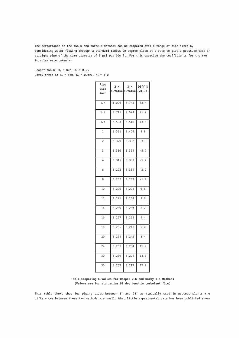
The performance of the two-K and three-K methods can be compared over a range of pipe sizes by considering water flowing through a standard radius 90 degree elbow at a rate to give a pressure drop instraight pipe of the same diameter of 3 psi per 100 ft. For this exercise the coefficients for the two formulas were taken as

Hooper two-K: K1 = 800, K∞ = 0.25Darby three-K: Km = 800, Ki = 0.091, Kd = 4.0

PipeSizeinch

2-KK-Value

3-KK-Value

Diff %(2K-3K)

1/4 1.096 0.743 38.4

1/2 0.715 0.574 21.9

3/4 0.593 0.516 13.8

1 0.501 0.463 8.0

2 0.379 0.392 -3.3

3 0.336 0.355 -5.7

4 0.315 0.333 -5.7

6 0.293 0.304 -3.9

8 0.282 0.287 -1.7

10 0.276 0.274 0.6

12 0.271 0.264 2.6

14 0.269 0.260 3.7

16 0.267 0.253 5.4

18 0.265 0.247 7.0

20 0.264 0.242 8.4

24 0.261 0.234 11.0

30 0.259 0.224 14.5

36 0.257 0.217 17.0

Table Comparing K-Values for Hooper 2-K and Darby 3-K Methods(Values are for std radius 90 deg bend in turbulent flow)

This table shows that for piping sizes between 1" and 24" as typically used in process plants thedifferences between these two methods are small. What little experimental data has been published shows

larger variations than the differences between these two methods, and suggests that both these methodsare slightly conservative.

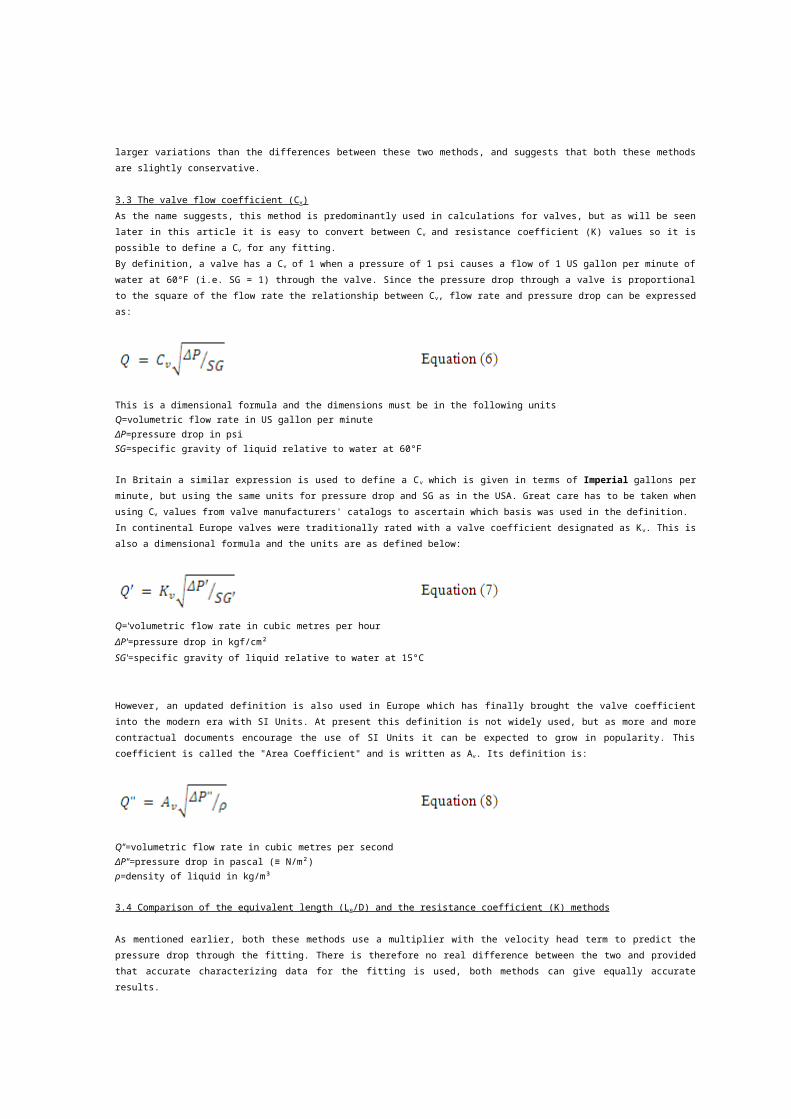
3.3 The valve flow coefficient (Cv)As the name suggests, this method is predominantly used in calculations for valves, but as will be seenlater in this article it is easy to convert between Cv and resistance coefficient (K) values so it ispossible to define a Cv for any fitting.By definition, a valve has a Cv of 1 when a pressure of 1 psi causes a flow of 1 US gallon per minute ofwater at 60°F (i.e. SG = 1) through the valve. Since the pressure drop through a valve is proportionalto the square of the flow rate the relationship between Cv, flow rate and pressure drop can be expressedas:

This is a dimensional formula and the dimensions must be in the following unitsQ=volumetric flow rate in US gallon per minuteΔP=pressure drop in psiSG=specific gravity of liquid relative to water at 60°F

In Britain a similar expression is used to define a Cv which is given in terms of Imperial gallons perminute, but using the same units for pressure drop and SG as in the USA. Great care has to be taken whenusing Cv values from valve manufacturers' catalogs to ascertain which basis was used in the definition.In continental Europe valves were traditionally rated with a valve coefficient designated as Kv. This isalso a dimensional formula and the units are as defined below:

Q='volumetric flow rate in cubic metres per hourΔP'=pressure drop in kgf/cm²SG'=specific gravity of liquid relative to water at 15°C

However, an updated definition is also used in Europe which has finally brought the valve coefficientinto the modern era with SI Units. At present this definition is not widely used, but as more and morecontractual documents encourage the use of SI Units it can be expected to grow in popularity. Thiscoefficient is called the "Area Coefficient" and is written as Av. Its definition is:

Q"=volumetric flow rate in cubic metres per secondΔP"=pressure drop in pascal (≡ N/m²)ρ=density of liquid in kg/m³

3.4 Comparison of the equivalent length (Le/D) and the resistance coefficient (K) methods

As mentioned earlier, both these methods use a multiplier with the velocity head term to predict thepressure drop through the fitting. There is therefore no real difference between the two and providedthat accurate characterizing data for the fitting is used, both methods can give equally accurateresults.

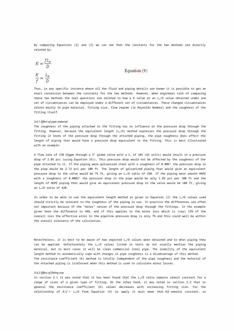
By comparing Equations (2) and (3) we can see that the constants for the two methods are directlyrelated by:

Thus, in any specific instance where all the fluid and piping details are known it is possible to get anexact conversion between the constants for the two methods. However, when engineers talk of comparingthese two methods the real questions are related to how a K value or an Le/D value obtained under oneset of circumstances can be employed under a different set of circumstances. These changed circumstancesrelate mainly to pipe material, fitting size, flow regime (ie Reynolds Number) and the roughness of thefitting itself.

3.4.1 Effect of pipe materialThe roughness of the piping attached to the fitting has no influence on the pressure drop through thefitting. However, because the equivalent length (Le/D) method expresses the pressure drop through thefitting in terms of the pressure drop through the attached piping, the pipe roughness does affect thelength of piping that would have a pressure drop equivalent to the fitting. This is best illustratedwith an example:

A flow rate of 150 USgpm through a 3" globe valve with a Cv of 105 (US units) would result in a pressuredrop of 2.05 psi (using Equation (6)). This pressure drop would not be affected by the roughness of thepipe attached to it. If the piping were galvanized steel with a roughness of 0.006" the pressure drop inthe pipe would be 2.72 psi per 100 ft. The length of galvanized piping that would give an equivalentpressure drop to the valve would be 75 ft, giving an Le/D ratio of 290. If the piping were smooth HDPEwith a roughness of 0.0002" the pressure drop in the pipe would be only 1.89 psi per 100 ft and thelength of HDPE piping that would give an equivalent pressure drop to the valve would be 108 ft, givingan Le/D ratio of 420.

In order to be able to use the equivalent length method as given in Equation (2) the Le/D values usedshould strictly be relevant to the roughness of the piping in use. In practice the differences are oftennot important because of the "minor" nature of the pressure drop through the fittings. In the examplegiven here the difference is 44%, and if this applies to the minor loss which is (say) 15% of theoverall loss the effective error in the pipeline pressure drop is only 7% and this could well be withinthe overall tolerance of the calculation.

Nevertheless, it is best to be aware of how reported Le/D values were obtained and to what piping theycan be applied. Unfortunately the Le/D values listed in texts do not usually mention the pipingmaterial, but in most cases it will be clean commercial steel pipe. The inability of the equivalentlength method to automatically cope with changes in pipe roughness is a disadvantage of this method.The resistance coefficient (K) method is totally independent of the pipe roughness and the material ofthe attached piping is irrelevant when this method is used to calculate minor losses.

3.4.2 Effect of fitting sizeIn section 3.1 it was noted that it has been found that the Le/D ratio remains almost constant for arange of sizes of a given type of fitting. On the other hand, it was noted in section 3.2 that ingeneral the resistance coefficient (K) values decreases with increasing fitting size. For therelationship of K/ƒ = Le/D from Equation (9) to apply it must mean that K/ƒ remains constant, or

that K and ƒ change at the same rate. This observation was the basis of the Crane K method and isdiscussed further in section 4 below.When using the equivalent length method, the (Le/D) ratio is multiplied by the friction factor and sincethe friction factor decreases as the pipe size increases the term (ƒLe/D) decreases accordingly. Thismakes the equivalent length method largely self-correcting for changes in fitting size and makes it verysuitable for preliminary or hand calculations where ultimate accuracy is not the main goal.The best available method available at present to accommodate changing pipe sizes appears to be Darby's3-K method. This method predicts resistance coefficients slightly higher than some of the older datathat did take fitting size into account (for example, the Hydraulic Institute "Pipe Friction Manual")but because it is given in algebraic form it is much easier to use in modern spreadsheets and computerprograms than the graphical data presented in the older documents.As an illustration, consider 2" and 20" long radius bends in a clean commercial steel pipeline. At fullyturbulent flow the resistance coefficient (K) calculated by the Darby method would be 0.274 for the 2"bend and 0.173 for the 20". This is a 37% decrease. If the equivalent length is calculated from these Kvalues and from the Moody friction factor for clean commercial steel pipe then the 2" bend has an (Le/D)value of 13.8 and the 20" bend has value of 14.0 - a change of just over 1% and a strong recommendationfor the equivalent length method.

3.4.3 Effect of flow regime (Reynolds Number)The early "classic" K values were measured under fully turbulent flow conditions. This is the flowregime most often used in industrial applications and it was an understandable place to startaccumulating data. But it was observed that at lower Reynolds Numbers in the transition zone between Re= 4,000 and fully developed turbulent flow the K values did increase somewhat. When the investigationswere extended into the laminar regime very large K value increases were found.Continuing with the example of the long radius bends, at a Reynolds number of 100 the Darby 3-K methodpredicts that both the 2" and the 20" L.R. bends would have K values of 8.2. This is a huge increaseover the turbulent flow situation. It should be remembered though that in the laminar flow regimevelocities tend to be very low, making the velocity head (v2/2g) low and since the pressure drop iscalculated as the product of the K value and the velocity head, the effect of the increase in K ispartially offset and the pressure drop can be low in absolute terms.Again, the equivalent lengths can be calculated from these K values and the Moody friction factors togive an (Le/D) ratio and this turns out to be 12.8 for both bends. This small change in the (Le/D) ratiocompared with those found in section 3.4.2, despite such a large change in Reynolds number, furtherreinforces the equivalent length method as a very useful technique for preliminary and non-missioncritical calculations.There is another consideration of the flow regime that arises out of engineering convention, rather thanfrom fundamentals. Strictly, the velocity head (the kinetic energy term in the Bernoulli equation)should be expressed as (αv2/2g). The correction factor, α, is required because by convention the velocityis taken as the average velocity (i.e. v = flow rate / cross sectional area). In reality (averagevelocity)2 is not equal to (average of v2) and the correction factor is used to avoid having to integrateto get the true average. In turbulent flow α is very close to 1 and in laminar flow it has a value of 2.It was stated in section 2 above that to calculate the pressure drop in straight pipe the velocity headis multiplied by the factor (ƒL/D). There is no α in the Darcy-Weisbach formula (Equation (1)), so whatdo we do for laminar flow? The answer is that by engineering convention the effect of α is absorbed intothe friction factor. We could include α and use a friction factor that is only half the usual value, butto keep the arithmetic easy α is absorbed into the friction factor, ƒ, and the velocity head is taken as(v2/2g).A similar thing is done with the resistance coefficients (K values) for pipe fittings. We define the Kvalues to include the value of α just to keep the arithmetic easy.There is one exception when it comes to minor losses. What is often called the "exit loss", but which ismore accurately the acceleration loss, is the kinetic energy in the stream issuing from the discharge ofthe pipe. This energy is lost and is equal to one velocity head. There is no way of getting away from itthat here you have to use the correct value of α to get the "exit loss" correct. The only alternativewould be to define it to have a K value of 2 in laminar flow, but it would then appear that in laminarflow you lose 2 velocity heads.

In practice this is usually not important. In laminar flow the velocity is low enough that one velocityhead is insignificant - and even if doubled with an α value of 2, it is still insignificant. The Kvalues of fittings in laminar flow can go into the hundreds, or even thousands, and one measly little2.0 isn't going to bother anybody.

3.4.4 Effect of the fitting roughnessThe main causes of the pressure losses in pipe fittings are the changes in direction and cross sectionalarea. Both of these changes result in acceleration of the fluid and this consumes energy. There will ofcourse be some influence of the friction between the inner surface of the fitting and the fluid on thepressure drop through the fitting, but it needs to be seen in context. Sticking with the example of theL.R. bend, the flow path through the bend can be calculated to be approximately 2.5 times the insidediameter of the pipe.

The equivalent length of a long radius bend is usually taken (perhaps a bit conservatively) as 16. Ifthe overall pressure drop is equivalent to a pipe length of 16 diameters, and the pressure drop due tothe actual flow path length (which is affected by the roughness) is equivalent to only 2.5 diametersthen it can be seen that a small change in the wall friction inside the bend will have a very smalleffect on the total pressure drop. In a higher resistance fitting like a globe valve or strainer theeffect of the friction is even less.

Experimental work on flow in bends has shown that the roughness does have a measurable impact on thepressure drop. But the experimental work also shows that there are measurable differences in thepressure drop through supposedly identical fittings from different manufacturers. Because thedifferences are small, all the generally accepted methods have ignored the roughness in the fitting andhave rather selected slightly conservative values for (Le/D) and (K).

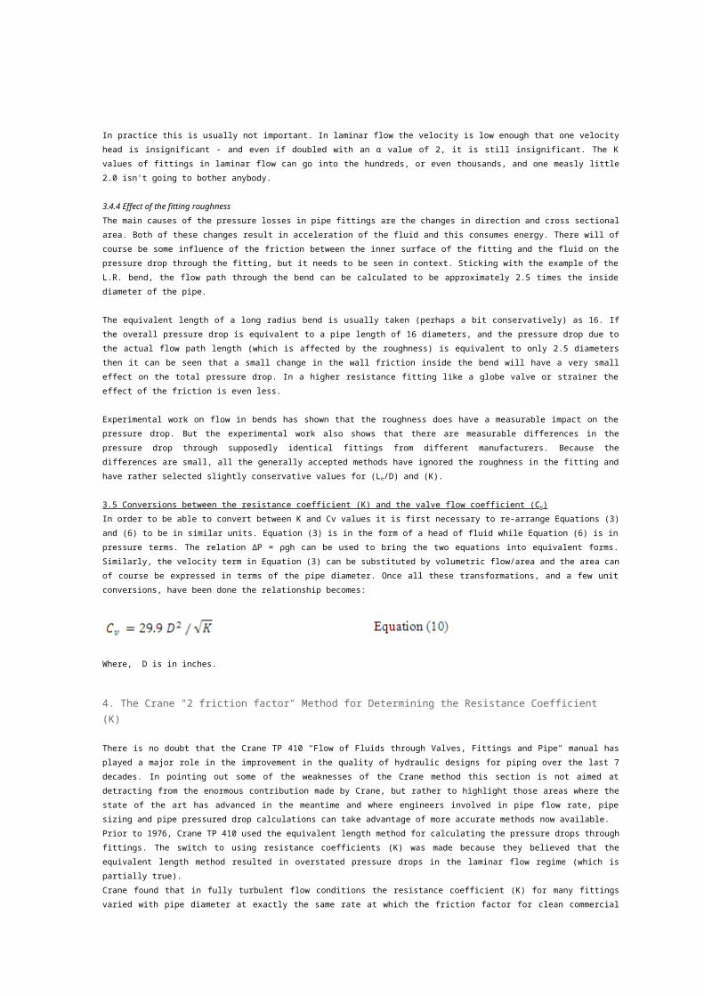
3.5 Conversions between the resistance coefficient (K) and the valve flow coefficient (Cv)In order to be able to convert between K and Cv values it is first necessary to re-arrange Equations (3)and (6) to be in similar units. Equation (3) is in the form of a head of fluid while Equation (6) is inpressure terms. The relation ΔP = ρgh can be used to bring the two equations into equivalent forms.Similarly, the velocity term in Equation (3) can be substituted by volumetric flow/area and the area canof course be expressed in terms of the pipe diameter. Once all these transformations, and a few unitconversions, have been done the relationship becomes:

Where, D is in inches.

4. The Crane "2 friction factor" Method for Determining the Resistance Coefficient (K)

There is no doubt that the Crane TP 410 "Flow of Fluids through Valves, Fittings and Pipe" manual hasplayed a major role in the improvement in the quality of hydraulic designs for piping over the last 7decades. In pointing out some of the weaknesses of the Crane method this section is not aimed atdetracting from the enormous contribution made by Crane, but rather to highlight those areas where thestate of the art has advanced in the meantime and where engineers involved in pipe flow rate, pipesizing and pipe pressured drop calculations can take advantage of more accurate methods now available.Prior to 1976, Crane TP 410 used the equivalent length method for calculating the pressure drops throughfittings. The switch to using resistance coefficients (K) was made because they believed that theequivalent length method resulted in overstated pressure drops in the laminar flow regime (which ispartially true).Crane found that in fully turbulent flow conditions the resistance coefficient (K) for many fittingsvaried with pipe diameter at exactly the same rate at which the friction factor for clean commercial

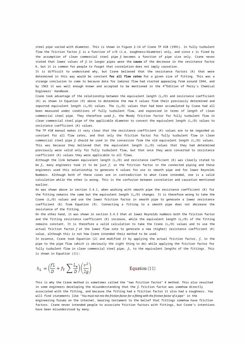
steel pipe varied with diameter. This is shown in Figure 2-14 of Crane TP 410 (1991). In fully turbulentflow the friction factor ƒT is a function of ε/D (i.e. roughness/diameter) only, and since ε is fixed bythe assumption of clean commercial steel pipe ƒT becomes a function of pipe size only. Crane neverstated that lower values of ƒT in larger pipes were the cause of the decrease in the resistance factorK, but it is common for people to forget that correlation does not imply causation.It is difficult to understand why, but Crane believed that the resistance factors (K) that weredetermined in this way would be constant for all flow rates for a given size of fitting. This was astrange conclusion to come to because data for laminar flow had started appearing from around 1944, andby 1963 it was well enough known and accepted to be mentioned in the 4thEdition of Perry's ChemicalEngineers' Handbook.Crane took advantage of the relationship between the equivalent length (Le/D) and resistance coefficient(K) as shown in Equation (9) above to determine the new K values from their previously determined andreported equivalent length (Le/D) values. The (Le/D) values that had been accumulated by Crane had allbeen measured under conditions of fully turbulent flow, and expressed in terms of length of cleancommercial steel pipe. They therefore used ƒT, the Moody friction factor for fully turbulent flow inclean commercial steel pipe of the applicable diameter to convert the equivalent length (Le/D) values toresistance coefficient (K) values.The TP 410 manual makes it very clear that the resistance coefficient (K) values are to be regarded asconstant for all flow rates, and that only the friction factor for fully turbulent flow in cleancommercial steel pipe ƒT should be used in the conversion from the old equivalent length (Le/D) values.This was because they believed that the equivalent length (Le/D) values that they had determinedpreviously were valid only for fully turbulent flow, but that once they were converted to resistancecoefficient (K) values they were applicable to all flows.Although the link between equivalent length (Le/D) and resistance coefficient (K) was clearly stated tobe ƒT, many engineers took it to be just ƒ, or the friction factor in the connected piping and theseengineers used this relationship to generate K values for use in smooth pipe and for lower ReynoldsNumbers. Although both of these cases are in contradiction to what Crane intended, one is a validcalculation while the other is wrong. This is the confusion between correlation and causation mentionedearlier.As was shown above in section 3.4.1, when working with smooth pipe the resistance coefficient (K) forthe fitting remains the same but the equivalent length (Le/D) changes. It is therefore wrong to take theCrane (Le/D) values and use the lower friction factor in smooth pipe to generate a lower resistancecoefficient (K) from Equation (9). Connecting a fitting to a smooth pipe does not decrease theresistance of the fitting.On the other hand, it was shown in section 3.4.3 that at lower Reynolds numbers both the friction factorand the fitting resistance coefficient (K) increase, while the equivalent length (Le/D) of the fittingremains constant. It is therefore a valid calculation to take the Crane (Le/D) values and to use theactual friction factor ƒ at the lower flow rate to generate a new (higher) resistance coefficient (K)value, although this is not how Crane intended their method to be used.In essence, Crane took Equation (2) and modified it by applying the actual friction factor, ƒ, in thepipe to the pipe flow (which is obviously the right thing to do) while applying the friction factor forfully turbulent flow in clean commercial steel pipe, ƒT, to the equivalent lengths of the fittings. Thisis shown in Equation (11):

This is why the Crane method is sometimes called the "two friction factor" K method. This also resulted in some engineers developing the misunderstanding that the ƒT friction factor was somehow directly associated with the fitting, and because the fitting had a friction factor it also had a roughness. You will find statements like "You must not mix the friction factor for a fitting with the friction factor of a pipe" in the engineering forums on the internet, bearing testament to the belief that fittings somehow have friction factors. Crane never intended people to associate friction factors with fittings, but Crane's intentionshave been misunderstood by many.

The result of the switch from the equivalent length (Le/D) method to the resistance coefficient (K)method was (apart from the confusion caused) that while the (Le/D) method may have overstated pressuredrops slightly in the laminar flow regime, the new constant K value method horribly understated them.The examples in sections 3.4.2 and 3.4.3 show how the resistance coefficient (K) for a L.R. bend canincrease from around 0.2 to 8.2 when the Reynolds Number drops to 100. Fortunately this error is usuallynot significant in practice because the pressure drops through the fittings tend to be a small part ofthe overall pressure drop, and a large error in a small portion becomes a small error overall.When Crane first published their piping design guidelines in 1935, industrial piping was manufacturedalmost exclusively from carbon steel and the Crane methods were aimed at providing reliable designmethods for that pipe. Also, the overwhelming majority of industrial pipe flow is in the turbulent flowregime. Crane certainly succeeded in establishing a comprehensive and accurate design method forturbulent flow in steel pipe. In modern times with the ever increasing use of smooth plastic and highalloy pipe it is essential that engineers fully understand the design methods they use, and that theyemploy the right method for the problem at hand. The right methods are available in the 2-K and 3-Kresistance coefficient methods discussed earlier, and it is time for the piping design world to breakwith the past and to embrace the new methods.

5. Accuracy

Much of what has been said above could be seen to imply that determining the pressure losses in pipefittings is an exact science. It is not. Very few sources of equivalent length (Le/D) or resistancecoefficient (K) values give accuracy or uncertainty limits. A notable exception is the HydraulicInstitute's Engineering Data Book. At the very best the uncertainty would be 10% and in general 25 to30% is probably a more realistic estimate.Standard fittings like elbows and tees vary from manufacturer to manufacturer and a tolerance of 25%should be assumed in calculations. Precision engineered items like control valves and metering orificeswill of course have much tighter tolerances, and these will usually be stated as part of theaccompanying engineering documentation.An area that needs particular care is using generic data for proprietary items. Many of the data tablesinclude values for proprietary items like gate, globe, butterfly and check valves, strainers and thelike. The actual flow data can vary very widely and variations of -50% to +100% from generic data can beexpected.

6. Conclusion

At some point in the past the equivalent length (Le/D) method of determining the pressure drop throughpipe fittings gained the reputation of being inaccurate. This was quite likely a result of Cranedropping this method in favour of the resistance coefficient (K) method. Recently this attitude haschanged in some circles, and hopefully the analysis done above will help convince more design engineersthat the equivalent length (Le/D) method is actually very useful and sufficiently accurate in manysituations. However, this method does suffer from two serious drawbacks. These are the necessity ofdefining the pressure drop properties of the fitting in terms of an arbitrary external factor (i.e. theattached piping) and the inability of this method to cope with entrances, exits and fittings with twocharacteristic diameters (e.g. changes in diameter and orifices). For these reasons the resistancecoefficient (K) method is the better route to accurate and comprehensive calculations.Darby's 3-K method has the capability of taking the fitting size and the flow regime into account. Thequantity of data available is gradually increasing and is now roughly equivalent in scope to the CraneTP 410 database. Already some of the higher end software has switched to using Darby's method, and itcan be expected that with time it will become more widely used.The data in Crane TP 410 remains a very valuable resource, but it should be used with an understandingof its range of applicability. Fortunately this data is at its most accurate in the zone of fullyturbulent flow, which is where most piping operates. The errors introduced by this method when the flowrate is below the fully turbulent regime can be large relative to the losses in the fittings themselves,

but since these are often a small part of the overall losses the errors are often insignificant. Asalways, an appreciation for the accuracy of the methods being employed enables the engineer to achieve asafe and economical design.

7. References

Crane Co. Flow of Fluids Through Valves, Fittings and Pipe. Tech Paper 410, 1991Darby, R. Chem Eng July, 1999, p. 101Darby, R. Chem Eng April, 2001, p. 127Hooper, WB. Chem Eng Aug 24, 1981, p. 97Hydraulic Institute, Pipe Friction Manual, New York 1954Hydraulic Institute, Engineering Data Book, 2nd ed, 1991Perry, JH. "Chemical Engineers' Handbook", 3rd ed, McGraw-Hill, 1950Perry, RH and Chilton, CH. "Chemical Engineers' Handbook", 4th ed, McGraw-Hill, 1963Perry, RH and Green, DW. "Chemical Engineers' Handbook", 7th ed, McGraw-Hill, 1997

Pipe Flow Calculations 3: The Friction Factor & Frictional Head Losswritten by: Harlan Bengtson • edited by: Lamar Stonecypher • updated:8/30/2010

Frictional head loss (or pressure drop) in pipe flow is related to thefriction factor and flow velocity by the Darcy Weisbach equation.Reynolds number is needed to find friction factor value. Fully developedturbulent flow is needed in order to use the friction factor equationfor pipe flow.

IntroductionPipe flow under pressure is used for a lot of purposes. Energy input tothe gas or liquid is needed to make it flow through the pipe or conduit.This energy input is needed because there is frictional energy loss(also called frictional head loss or frictional pressure drop) due tothe friction between the fluid and the pipe wall and internal frictionwithin the fluid. The Darcy Weisbach Equation, which will be discussedin this article, is commonly used for a variety of calculationsinvolving frictional head loss, pipe diameter, flow rate or velocity,and several other parameters. The friction factor, which is used in theDarcy Weisbach equation, depends upon the Reynolds number and the piperoughness.

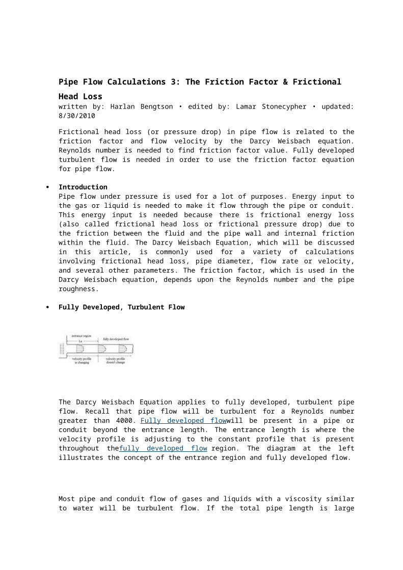
Fully Developed, Turbulent Flow

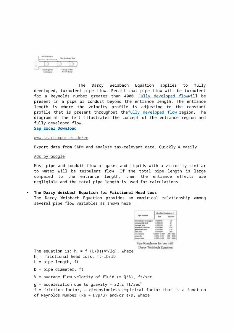
The Darcy Weisbach Equation applies to fullydeveloped, turbulent pipe flow. Recall that pipe flow will be turbulentfor a Reynolds number greater than 4000. Fully developed flowwill bepresent in a pipe or conduit beyond the entrance length. The entrancelength is where the velocity profile is adjusting to the constantprofile that is present throughout thefully developed flow region. Thediagram at the left illustrates the concept of the entrance region andfully developed flow.Sap Excel Download

www.smartexporter.de/en

Export data from SAP® and analyze tax-relevant data. Quickly & easily

Ads by Google

Most pipe and conduit flow of gases and liquids with a viscosity similarto water will be turbulent flow. If the total pipe length is largecompared to the entrance length, then the entrance effects arenegligible and the total pipe length is used for calculations.

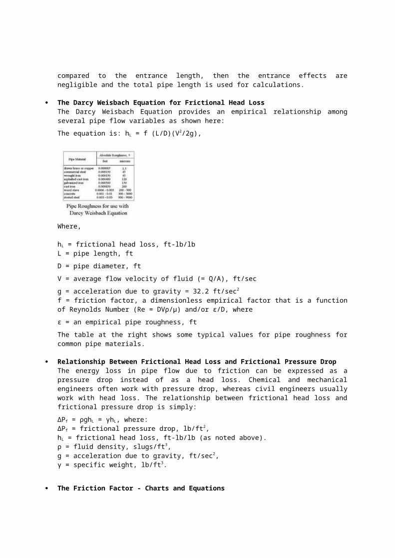
The Darcy Weisbach Equation for Frictional Head LossThe Darcy Weisbach Equation provides an empirical relationship amongseveral pipe flow variables as shown here:

The equation is: hL = f (L/D)(V2/2g), wherehL = frictional head loss, ft-lb/lbL = pipe length, ftD = pipe diameter, ftV = average flow velocity of fluid (= Q/A), ft/secg = acceleration due to gravity = 32.2 ft/sec2

f = friction factor, a dimensionless empirical factor that is a functionof Reynolds Number (Re = DVρ/μ) and/or ε/D, where

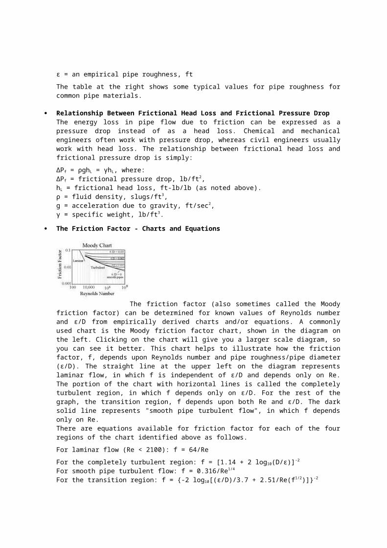
ε = an empirical pipe roughness, ftThe table at the right shows some typical values for pipe roughness forcommon pipe materials.

Relationship Between Frictional Head Loss and Frictional Pressure DropThe energy loss in pipe flow due to friction can be expressed as apressure drop instead of as a head loss. Chemical and mechanicalengineers often work with pressure drop, whereas civil engineers usuallywork with head loss. The relationship between frictional head loss andfrictional pressure drop is simply:ΔPf = ρghL = γhL, where:ΔPf = frictional pressure drop, lb/ft2,hL = frictional head loss, ft-lb/lb (as noted above).ρ = fluid density, slugs/ft3,g = acceleration due to gravity, ft/sec2,γ = specific weight, lb/ft3.

The Friction Factor - Charts and Equations

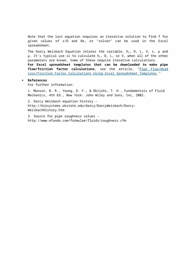
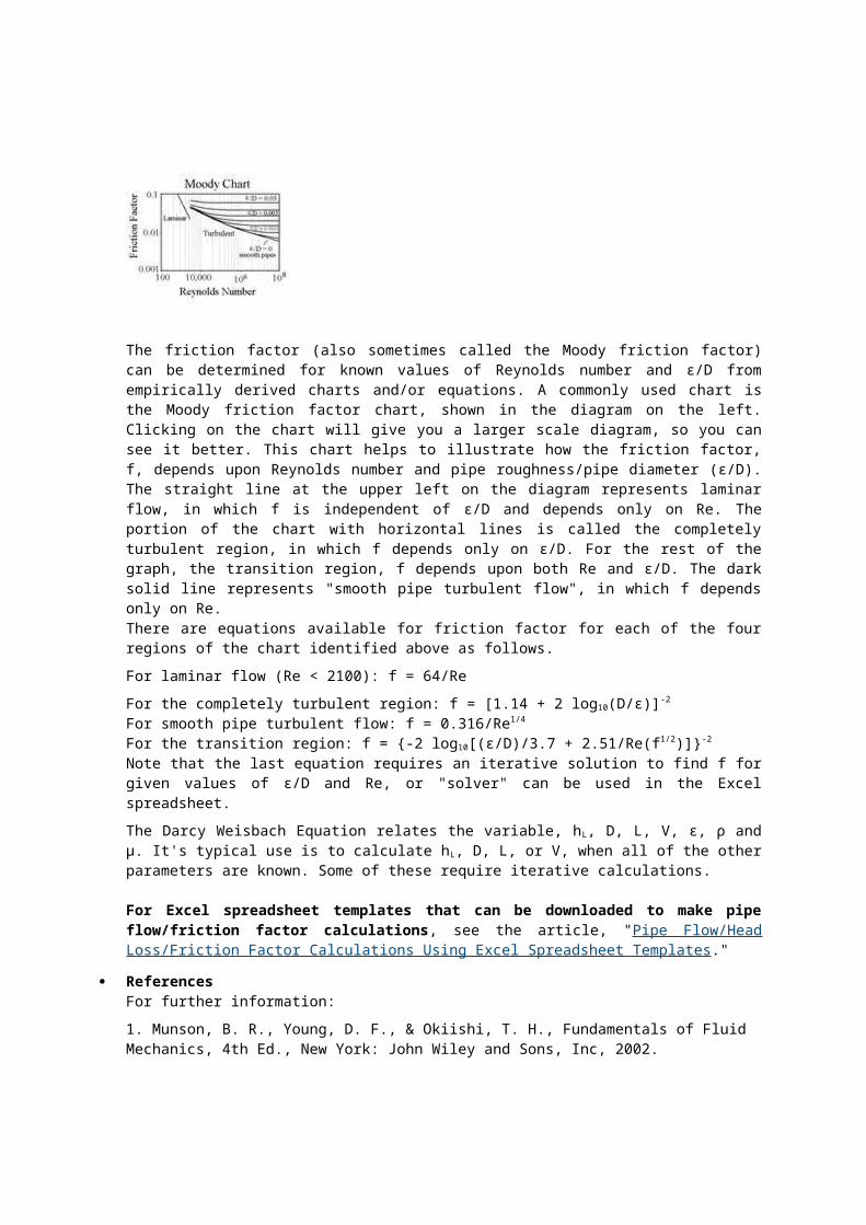
The friction factor (also sometimes called the Moodyfriction factor) can be determined for known values of Reynolds numberand ε/D from empirically derived charts and/or equations. A commonlyused chart is the Moody friction factor chart, shown in the diagram onthe left. Clicking on the chart will give you a larger scale diagram, soyou can see it better. This chart helps to illustrate how the frictionfactor, f, depends upon Reynolds number and pipe roughness/pipe diameter(ε/D). The straight line at the upper left on the diagram representslaminar flow, in which f is independent of ε/D and depends only on Re.The portion of the chart with horizontal lines is called the completelyturbulent region, in which f depends only on ε/D. For the rest of thegraph, the transition region, f depends upon both Re and ε/D. The darksolid line represents "smooth pipe turbulent flow", in which f dependsonly on Re.There are equations available for friction factor for each of the fourregions of the chart identified above as follows.For laminar flow (Re < 2100): f = 64/ReFor the completely turbulent region: f = [1.14 + 2 log10(D/ε)]-2

For smooth pipe turbulent flow: f = 0.316/Re1/4

For the transition region: f = {-2 log10[(ε/D)/3.7 + 2.51/Re(f1/2)]}-2

Note that the last equation requires an iterative solution to find f forgiven values of ε/D and Re, or "solver" can be used in the Excelspreadsheet.The Darcy Weisbach Equation relates the variable, hL, D, L, V, ε, ρ andμ. It's typical use is to calculate hL, D, L, or V, when all of the otherparameters are known. Some of these require iterative calculations.For Excel spreadsheet templates that can be downloaded to make pipeflow/friction factor calculations, see the article, "Pipe Flow/HeadLoss/Friction Factor Calculations Using Excel Spreadsheet Templates."

ReferencesFor further information:1. Munson, B. R., Young, D. F., & Okiishi, T. H., Fundamentals of Fluid Mechanics, 4th Ed., New York: John Wiley and Sons, Inc, 2002.2. Darcy Weisbach equation history - http://biosystems.okstate.edu/darcy/DarcyWeisbach/Darcy-WeisbachHistory.htm3. Source for pipe roughness values - http://www.efunda.com/formulae/fluids/roughness.cfm

Pipe Flow Calculations 1: the Entrance Length for Fully Developed Flowwritten by: Harlan Bengtson • edited by: Lamar Stonecypher • updated: 5/13/2010

The Reynolds number is used to calculate the entrance length needed toreach fully developed flow for turbulent flow or for laminar flow in apipe. At the end of the entrance length the pipe flow enters the fullydeveloped flow region, where the velocity profile remains constant.

IntroductionEquations for analyzing pipe flow, such as the Darcy Weisbach equationfor frictional head loss, often apply only to the fully developed flowportion of the pipe flow. If the total pipe length is large compared tothe entrance length, then the effect of the entrance length can usuallybe neglected and the total pipe length can be used in calculations. Ifthe total pipe length is relatively short in comparison with theentrance length, however, then the entrance region may need to beanalyzed separately. An estimate of the entrance length is sometimesneeded in order to determine how to proceed with pipe flow calculations.The Reynolds number for pipe flow is needed to calculate the entrancelength for turbulent flow or for laminar flow.

The Entrance Region

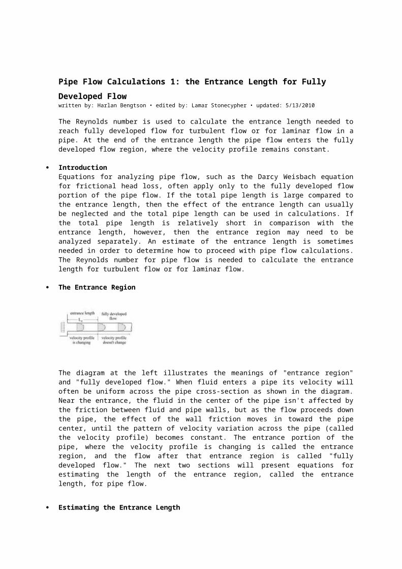
The diagram at the left illustrates the meanings of "entrance region"and "fully developed flow." When fluid enters a pipe its velocity willoften be uniform across the pipe cross-section as shown in the diagram.Near the entrance, the fluid in the center of the pipe isn't affected bythe friction between fluid and pipe walls, but as the flow proceeds downthe pipe, the effect of the wall friction moves in toward the pipecenter, until the pattern of velocity variation across the pipe (calledthe velocity profile) becomes constant. The entrance portion of thepipe, where the velocity profile is changing is called the entranceregion, and the flow after that entrance region is called "fullydeveloped flow." The next two sections will present equations forestimating the length of the entrance region, called the entrancelength, for pipe flow.

Estimating the Entrance Length

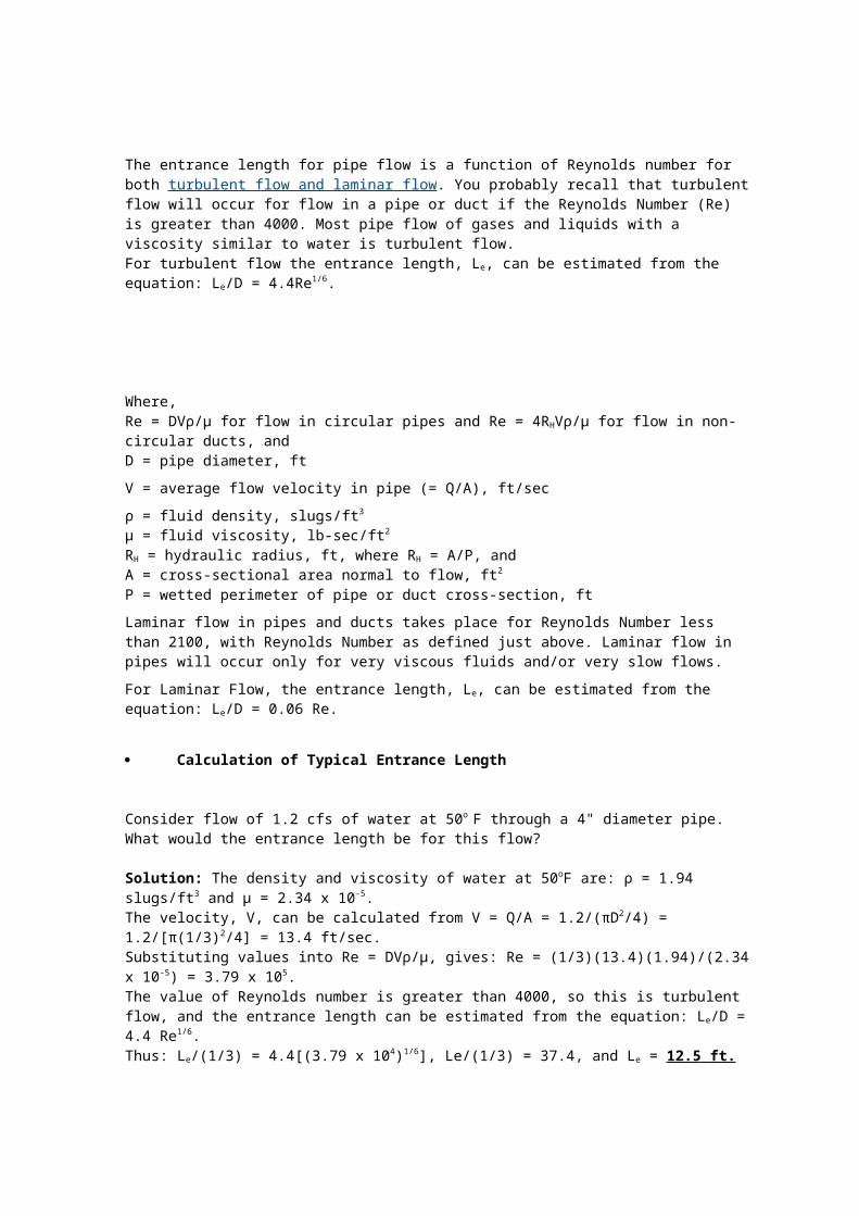
The entrance length for pipe flow is a function of Reynolds number for both turbulent flow and laminar flow. You probably recall that turbulentflow will occur for flow in a pipe or duct if the Reynolds Number (Re) is greater than 4000. Most pipe flow of gases and liquids with a viscosity similar to water is turbulent flow.For turbulent flow the entrance length, Le, can be estimated from the equation: Le/D = 4.4Re1/6.

Where, Re = DVρ/μ for flow in circular pipes and Re = 4RHVρ/μ for flow in non-circular ducts, andD = pipe diameter, ftV = average flow velocity in pipe (= Q/A), ft/secρ = fluid density, slugs/ft3

μ = fluid viscosity, lb-sec/ft2

RH = hydraulic radius, ft, where RH = A/P, andA = cross-sectional area normal to flow, ft2

P = wetted perimeter of pipe or duct cross-section, ftLaminar flow in pipes and ducts takes place for Reynolds Number less than 2100, with Reynolds Number as defined just above. Laminar flow in pipes will occur only for very viscous fluids and/or very slow flows.For Laminar Flow, the entrance length, Le, can be estimated from the equation: Le/D = 0.06 Re.

Calculation of Typical Entrance Length

Consider flow of 1.2 cfs of water at 50o F through a 4" diameter pipe. What would the entrance length be for this flow?

Solution: The density and viscosity of water at 50oF are: ρ = 1.94 slugs/ft3 and μ = 2.34 x 10-5.The velocity, V, can be calculated from V = Q/A = 1.2/(πD2/4) = 1.2/[π(1/3)2/4] = 13.4 ft/sec.Substituting values into Re = DVρ/μ, gives: Re = (1/3)(13.4)(1.94)/(2.34x 10-5) = 3.79 x 105.The value of Reynolds number is greater than 4000, so this is turbulent flow, and the entrance length can be estimated from the equation: Le/D = 4.4 Re1/6.Thus: Le/(1/3) = 4.4[(3.79 x 104)1/6], Le/(1/3) = 37.4, and Le = 12.5   ft.

Pipe Flow Calculations 2: Reynolds Number and Laminar & Turbulent FlowWritten by: Harlan Bengtson • edited by: Lamar Stonecypher • updated: 8/22/2010

Pipe flow may be either laminar flow or turbulent flow. Laminar flow ischaracterized by low flow velocity and high viscosity. Turbulent flow ischaracterized by high flow velocity and low viscosity. For Reynoldsnumber < 2100, flow is laminar. For Reynolds number > 4000, flow isturbulent.

IntroductionFor pipe flow applications, it's often important to be able to determinewhether a given flow condition is laminar flow or turbulent flow.Different equations or methods of analysis often apply to laminar flowand turbulent flow conditions.The concepts of turbulent and laminar flow are shown in the diagram inthe next section. Laminar flow (also called streamline flow or viscousflow) occurs for low Reynolds number, with relatively slow flow velocityand high viscosity It is characterized by all of the fluid velocityvectors lined up in the direction of flow. Turbulent flow, on the otherhand occurs at high Reynolds number, with relatively high flow velocityand low viscosity. It has point velocity vectors in all directions,although the overall flow is in one direction, along the axis of thepipe.Practical transport of water or air in a pipe or other closed conduit istypically turbulent flow. Similarly, pipe flow of other gases or liquidswith viscosity similar to water will normally be transported in conduitsunder turbulent flow conditions. Laminar flow will often be present withliquids of high viscosity, such as lubricating oils.

The Reynolds Number

The typical criterion for whether pipe flow is laminar or turbulent isthe value of the Reynolds Number. The Reynolds number for pipe flow isdefined as Re = DVρ/μ, where D is the pipe diameter, V is the averageflow velocity in the pipe, ρ is the density of the flowing fluid and μ

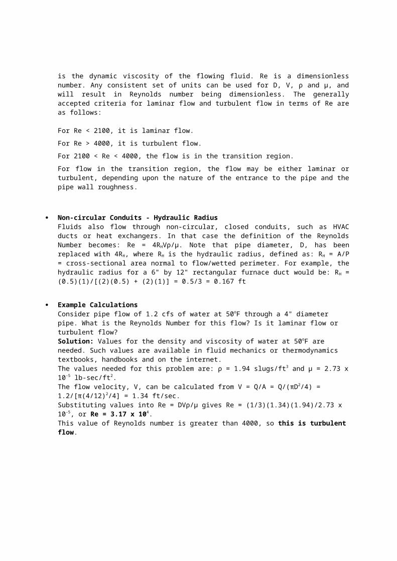
is the dynamic viscosity of the flowing fluid. Re is a dimensionlessnumber. Any consistent set of units can be used for D, V, ρ and μ, andwill result in Reynolds number being dimensionless. The generallyaccepted criteria for laminar flow and turbulent flow in terms of Re areas follows:

For Re < 2100, it is laminar flow.For Re > 4000, it is turbulent flow.For 2100 < Re < 4000, the flow is in the transition region.For flow in the transition region, the flow may be either laminar orturbulent, depending upon the nature of the entrance to the pipe and thepipe wall roughness.

Non-circular Conduits - Hydraulic RadiusFluids also flow through non-circular, closed conduits, such as HVACducts or heat exchangers. In that case the definition of the ReynoldsNumber becomes: Re = 4RHVρ/μ. Note that pipe diameter, D, has beenreplaced with 4RH, where RH is the hydraulic radius, defined as: RH = A/P= cross-sectional area normal to flow/wetted perimeter. For example, thehydraulic radius for a 6" by 12" rectangular furnace duct would be: RH =(0.5)(1)/[(2)(0.5) + (2)(1)] = 0.5/3 = 0.167 ft

Example CalculationsConsider pipe flow of 1.2 cfs of water at 50oF through a 4" diameter pipe. What is the Reynolds Number for this flow? Is it laminar flow or turbulent flow?Solution: Values for the density and viscosity of water at 50oF are needed. Such values are available in fluid mechanics or thermodynamics textbooks, handbooks and on the internet.The values needed for this problem are: ρ = 1.94 slugs/ft3 and μ = 2.73 x10-5 lb-sec/ft2.The flow velocity, V, can be calculated from V = Q/A = Q/(πD2/4) = 1.2/[π(4/12)2/4] = 1.34 ft/sec.Substituting values into Re = DVρ/μ gives Re = (1/3)(1.34)(1.94)/2.73 x 10-5, or Re = 3.17 x 104.This value of Reynolds number is greater than 4000, so this is turbulentflow.

Pipe Flow Calculations 3: The Friction Factor & Frictional Head Losswritten by: Harlan Bengtson • edited by: Lamar Stonecypher • updated:8/30/2010

Frictional head loss (or pressure drop) in pipe flow is related to thefriction factor and flow velocity by the Darcy Weisbach equation.Reynolds number is needed to find friction factor value. Fully developedturbulent flow is needed in order to use the friction factor equationfor pipe flow.

IntroductionPipe flow under pressure is used for a lot of purposes. Energy input tothe gas or liquid is needed to make it flow through the pipe or conduit.This energy input is needed because there is frictional energy loss(also called frictional head loss or frictional pressure drop) due tothe friction between the fluid and the pipe wall and internal frictionwithin the fluid. The Darcy Weisbach Equation, which will be discussedin this article, is commonly used for a variety of calculationsinvolving frictional head loss, pipe diameter, flow rate or velocity,and several other parameters. The friction factor, which is used in theDarcy Weisbach equation, depends upon the Reynolds number and the piperoughness.

Fully Developed, Turbulent Flow

The Darcy Weisbach Equation applies to fully developed, turbulent pipeflow. Recall that pipe flow will be turbulent for a Reynolds numbergreater than 4000. Fully developed flowwill be present in a pipe orconduit beyond the entrance length. The entrance length is where thevelocity profile is adjusting to the constant profile that is presentthroughout thefully developed flow region. The diagram at the leftillustrates the concept of the entrance region and fully developed flow.

Most pipe and conduit flow of gases and liquids with a viscosity similarto water will be turbulent flow. If the total pipe length is large

compared to the entrance length, then the entrance effects arenegligible and the total pipe length is used for calculations.

The Darcy Weisbach Equation for Frictional Head LossThe Darcy Weisbach Equation provides an empirical relationship amongseveral pipe flow variables as shown here:The equation is: hL = f (L/D)(V2/2g),

Where,

hL = frictional head loss, ft-lb/lbL = pipe length, ftD = pipe diameter, ftV = average flow velocity of fluid (= Q/A), ft/secg = acceleration due to gravity = 32.2 ft/sec2

f = friction factor, a dimensionless empirical factor that is a functionof Reynolds Number (Re = DVρ/μ) and/or ε/D, whereε = an empirical pipe roughness, ftThe table at the right shows some typical values for pipe roughness forcommon pipe materials.

Relationship Between Frictional Head Loss and Frictional Pressure DropThe energy loss in pipe flow due to friction can be expressed as apressure drop instead of as a head loss. Chemical and mechanicalengineers often work with pressure drop, whereas civil engineers usuallywork with head loss. The relationship between frictional head loss andfrictional pressure drop is simply:ΔPf = ρghL = γhL, where:ΔPf = frictional pressure drop, lb/ft2,hL = frictional head loss, ft-lb/lb (as noted above).ρ = fluid density, slugs/ft3,g = acceleration due to gravity, ft/sec2,γ = specific weight, lb/ft3.

The Friction Factor - Charts and Equations

The friction factor (also sometimes called the Moody friction factor)can be determined for known values of Reynolds number and ε/D fromempirically derived charts and/or equations. A commonly used chart isthe Moody friction factor chart, shown in the diagram on the left.Clicking on the chart will give you a larger scale diagram, so you cansee it better. This chart helps to illustrate how the friction factor,f, depends upon Reynolds number and pipe roughness/pipe diameter (ε/D).The straight line at the upper left on the diagram represents laminarflow, in which f is independent of ε/D and depends only on Re. Theportion of the chart with horizontal lines is called the completelyturbulent region, in which f depends only on ε/D. For the rest of thegraph, the transition region, f depends upon both Re and ε/D. The darksolid line represents "smooth pipe turbulent flow", in which f dependsonly on Re.There are equations available for friction factor for each of the fourregions of the chart identified above as follows.For laminar flow (Re < 2100): f = 64/ReFor the completely turbulent region: f = [1.14 + 2 log10(D/ε)]-2

For smooth pipe turbulent flow: f = 0.316/Re1/4

For the transition region: f = {-2 log10[(ε/D)/3.7 + 2.51/Re(f1/2)]}-2

Note that the last equation requires an iterative solution to find f forgiven values of ε/D and Re, or "solver" can be used in the Excelspreadsheet.The Darcy Weisbach Equation relates the variable, hL, D, L, V, ε, ρ andμ. It's typical use is to calculate hL, D, L, or V, when all of the otherparameters are known. Some of these require iterative calculations.

For Excel spreadsheet templates that can be downloaded to make pipeflow/friction factor calculations, see the article, "Pipe Flow/HeadLoss/Friction Factor Calculations Using Excel Spreadsheet Templates."

ReferencesFor further information:1. Munson, B. R., Young, D. F., & Okiishi, T. H., Fundamentals of Fluid Mechanics, 4th Ed., New York: John Wiley and Sons, Inc, 2002.

2. Darcy Weisbach equation history - http://biosystems.okstate.edu/darcy/DarcyWeisbach/Darcy-WeisbachHistory.htm3. Source for pipe roughness values - http://www.efunda.com/formulae/fluids/roughness.cfm

Excel Formulas to Calculate Water Flow Rates for Different Pipe SizesWritten by: Harlan Bengtson • edited by: Lamar Stonecypher • updated: 5/26/2011

Excel formulas to calculate water flow rates for pipe sizes (diameters and lengths) can be downloaded as Excel templates in this article. The Hazen Williams formula is used for water flow rate calculations. Either S.I. units or U.S. units can be used in the Excel spreadsheet templates.

Limitations on the Hazen Williams Formula for Water Flow Rate

CalculationsThe Hazen Williams formula is an empirical equation that can be used forturbulent flow of water at typical ambient temperatures. The turbulent flow requirement is not very limiting. Most practical applications of water transport in pipes are in the turbulent flow regime. For a review of this topic see the article, 'Reynolds Number and Laminar & Turbulent Flow.' Strictly speaking, the Hazen Williams formula applies to water at60oF, but it works quite well for a reasonable range of water temperatures above or below 60oF. For fluids with viscosity different from water, or for water temperatures far above or below 60oF, the Darcy Weisbach Equation works better than the Hazen Williams Formula. Click onthe following link for more details about the Darcy Weisbach Equation.Following presentation and discussion of several forms of the Hazen Williams equation in the next couple of sections, a downloadable Excel spreadsheet template will be presented and discussed for making Hazen Williams water flow rate calculations, using Excel formulas.

Forms of the Hazen Williams FormulaThere are several different forms of the Hazen Williams Formula in use for water flow rate calculations. It can be written in terms of water velocity or water flow rate, in terms of pressure drop or head loss, andfor several different sets of units. The traditional form of the Hazen Williams formula is:U.S. units: V = 1.318 C R0.633 S0.54,

Where: V = water flow velocity in ft/sec C = Hazen Williams coefficient, dependent on the pipe material and

pipe age R = Hydraulic radius, ft (R = cross-sectional area/wetted perimeter) S = slope of energy grade line = head loss/pipe length = hL/L, which

is dimensionlessS.I. units: V = 0.85 C R0.633 S0.54, where: V is in m/s and R is in metersThe Hazen Williams Formula is used primarily for pressure flow in pipes,for which the hydraulic radius is one fourth of the pipe diameter (R = D/4). Using this relationship and Q = V(πD2/4), for flow in a circular pipe, the Hazen Williams formula can be rewritten as shown in the next section.

Water Flow Rates for Pipe Sizes over a Range of Diameters with the Hazen

Williams FormulaFor flow of water under pressure in a circular pipe, the Hazen Williams formula shown above can be rewritten into the following convenient form:in U.S. units: Q = 193.7 C D2.63 S0.54, where: Q = water flow rate in gal/min (gpm) D = pipe diameter in ft C and S are the same as abovein S.I. units: Q = 0.278 C D2.63 S0.54, where Q is in m3/s and D is in metersThe Hazen Williams formula can also be expressed in terms of the pressure difference (ΔP) instead of head loss (hL) across the pipe length, L, using ΔP = ρghL:In S.I. units, a convenient form of the equation is: Q = (3.763 x 10-6) CD2.63 (ΔP/L)0.54, where Q is water flow rate in m3/hr, D is pipe diameter in mm L is pipe length in m, ΔP is the pressure difference across pipe length, L, in kN/m2

In U.S. units: Q = 0.442 C D2.63 (ΔP/L)0.54, where Q is water flow rate in gpm, D is pipe diameter in inches L is pipe length in ft, ΔP is the pressure difference across pipe length, L, in psiThis is a form of the Hazen Williams formula that is convenient to use for estimating water flow rates for pipe sizes and lengths in U.S. units, as illustrated in the section after next on the second page.The second page of this article has a table with values for the Hazen Williams coefficient, a table with example water flow rate calculations for several PVC pipe lengths and diameters, and a link to download a spreadsheet template with Excel formulas to make the water flow rate calculations.

Values for the Hazen Williams Coefficient

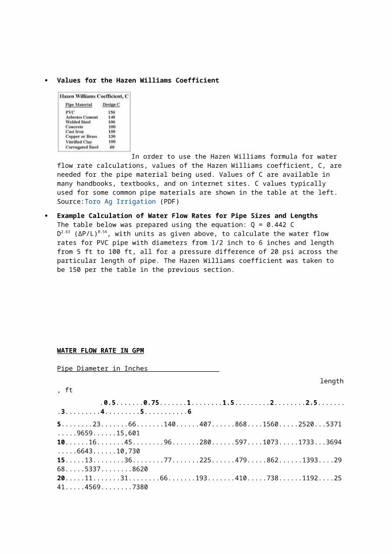
In order to use the Hazen Williams formula for water flow rate calculations, values of the Hazen Williams coefficient, C, areneeded for the pipe material being used. Values of C are available in many handbooks, textbooks, and on internet sites. C values typically used for some common pipe materials are shown in the table at the left.Source:Toro Ag Irrigation (PDF)

Example Calculation of Water Flow Rates for Pipe Sizes and LengthsThe table below was prepared using the equation: Q = 0.442 C D2.63 (ΔP/L)0.54, with units as given above, to calculate the water flow rates for PVC pipe with diameters from 1/2 inch to 6 inches and length from 5 ft to 100 ft, all for a pressure difference of 20 psi across the particular length of pipe. The Hazen Williams coefficient was taken to be 150 per the table in the previous section.

WATER FLOW RATE IN GPM

Pipe Diameter in Inches length, ft .0.5.......0.75.......1........1.5.........2........2.5........3.........4.........5...........65........23.......66.......140......407......868....1560.....2520...5371.....9659......15,60110......16.......45........96.......280......597....1073.....1733...3694.....6643......10,73015.....13........36........77.......225......479.....862......1393....2968.....5337........862020.....11.......31........66.......193.......410.....738......1192....2541.....4569........7380

40.....7.........21........46.......132......282......508......820.....1747.....3142........5076100...4.........13........28........81.......172.....309.......500.....1065.....1916........3096

The table shows a pattern that you should intuitively expect. For agiven pressure difference driving the flow, the water flow rateincreases as diameter increases for a given pipe length and the waterflow rate decreases as pipe length increases for a given pipe diameter.The equation above can be used to calculate water flow rates for pipesizes and lengths with different pipe materials and pressure drivingforces, using the Hazen Williams equation as demonstrated in the tableabove.

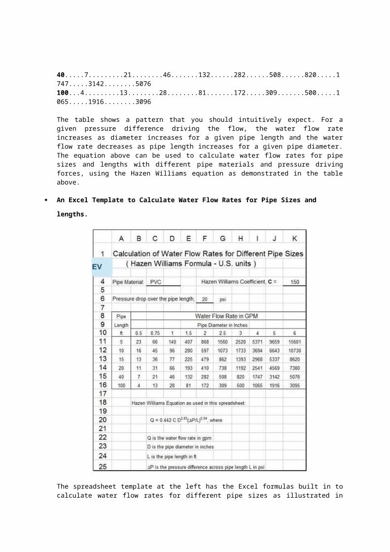
An Excel Template to Calculate Water Flow Rates for Pipe Sizes and

lengths.

The spreadsheet template at the left has the Excel formulas built in tocalculate water flow rates for different pipe sizes as illustrated in

the previous section. This Excel spreadsheet template that can bedownloaded below, allows for input of the Hazen Williams coefficientvalue and the pressure drop across the length of pipe being considered.Also, the pipe diameters and lengths can be changed from those currentlyin the spreadsheet, so the flow rate can be calculated for anycombination of pipe diameter and length if the Hazen Williamscoefficient is known and the pressure drop across the pipe is known.The example spreadsheet has U.S. units, but an S.I. version and a U.S.version are available for download.

ReferencesReferences for Further Information:1. Bengtson, H., Fundamentals of Fluid Flow, An online continuing education course for PDH credit.2. Munson, B. R., Young, D. F., & Okiishi, T. H., Fundamentals of Fluid Mechanics, 4th Ed., New York: John Wiley and Sons, Inc, 2002.3. Liou, C.P., "Limitations and Proper Use of the Hazen-Williams Equation," Journal of Hydraulic Engineering, Vol. 124, No. 9, Sept. 1998, pp. 951-954.

Natural Convection Heat Transfer Coefficient Estimation Calculationswritten by: Harlan Bengtson • edited by: Lamar Stonecypher • updated: 9/25/2013

Download Excel spreadsheets to calculate natural convection heat transfer coefficients. We've included several configurations, including vertical plate or from a horizontal cylinder.

Newton’s Law of Cooling for Forced and Natural Convection Heat TransferConvection heat transfer takes place when a fluid flows past a solid surface, with a difference in temperature between the fluid and the surface. If the fluid flow is due to an external force, like a pump or fan, it is forced convection. If the fluid flow is caused by density differences within the fluid due to internal fluid temperature differences, then it is natural convection, also sometimes called free convection.An equation that is widely used for both forced and natural convection heat transfer is Newton's Law of Cooling: Q = h A ΔT, whereQ is the rate of heat transfer between the fluid and the surface, Btu/hr(W for S.I.),

A is the area of the surface that is in contact with the fluid, ft2 (m2 for S.I.),ΔT is the temperature difference between the fluid and the solid surface, oF (oC or K for S.I.),h is the convective heat transfer coefficient, Btu/hr-ft2-oF (W/m2-K for S.I.)

Determining the value for the heat transfer coefficient is the major part of convective heat transfer calculations. The article, "Calculationof Forced Convection Heat Transfer Coefficients with Excel Spreadsheets," provides information about correlations and Excel spreadsheets to calculate heat transfer coefficients for several forced convection heat transfer configurations. This article provides similar information and Excel spreadsheets to calculate natural convection heat transfer coefficients.

Dimensionless Prandtl, Grashof, Rayleigh and Nusselt NumbersThe equations used to calculate natural convection heat transfer coefficients come from correlations of dimensionless numbers. The

dimensionless  numbers typically appearing in these correlations are the Nusselt number, the Prandtl number, the Grashof number, and sometimes the Rayleigh number. The equations for the Nusselt, Prandtl, and Grashof numbers (Nu, Pr, and Gr) are shown in the box at the right. The Rayleigh number is simply: Ra = Gr Pr.Following are the parameters that appear in these dimensionless numbers (units are given for the U.S engineering system with S.I. units in parentheses): D is a characteristic length parameter (e.g. diameter for natural

convection from a circular cylinder or a sphere or height of a vertical plate) in ft (m for S.I.)

ρ is the density of the fluid in slugs/ft3 (Kg/m3 for S.I.) μ is the viscosity of the fluid in lb-sec/ft2 (N-s/m2 for S.I.) k is the thermal conductivity of the fluid in Btu/hr-ft-oF (W/m-K for

S.I.) Cp is the heat capacity of the fluid in Btu/lb-oF (J/kg-K for S.I.) g is the acceleration due to gravity (32.17 ft/sec2 or 9.81 m/s2)

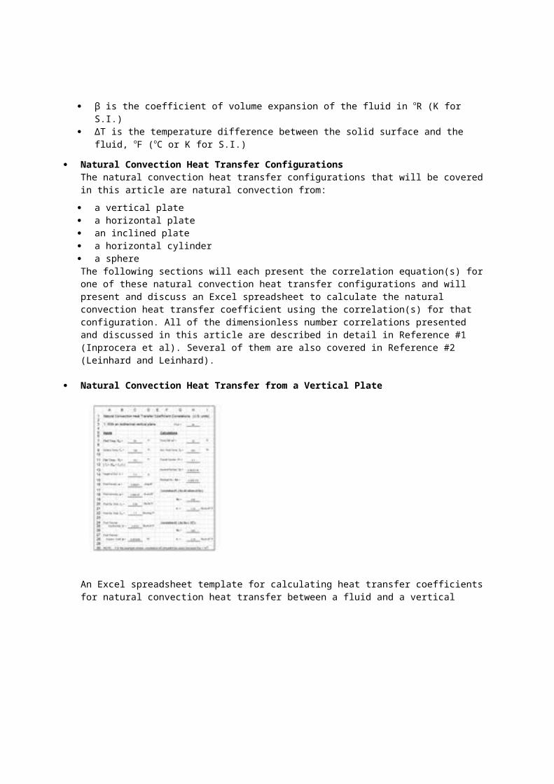
β is the coefficient of volume expansion of the fluid in oR (K for S.I.)

ΔT is the temperature difference between the solid surface and the fluid, oF (oC or K for S.I.)

Natural Convection Heat Transfer ConfigurationsThe natural convection heat transfer configurations that will be coveredin this article are natural convection from: a vertical plate a horizontal plate an inclined plate a horizontal cylinder a sphereThe following sections will each present the correlation equation(s) forone of these natural convection heat transfer configurations and will present and discuss an Excel spreadsheet to calculate the natural convection heat transfer coefficient using the correlation(s) for that configuration. All of the dimensionless number correlations presented and discussed in this article are described in detail in Reference #1 (Inprocera et al). Several of them are also covered in Reference #2 (Leinhard and Leinhard).

Natural Convection Heat Transfer from a Vertical Plate

An Excel spreadsheet template for calculating heat transfer coefficientsfor natural convection heat transfer between a fluid and a vertical

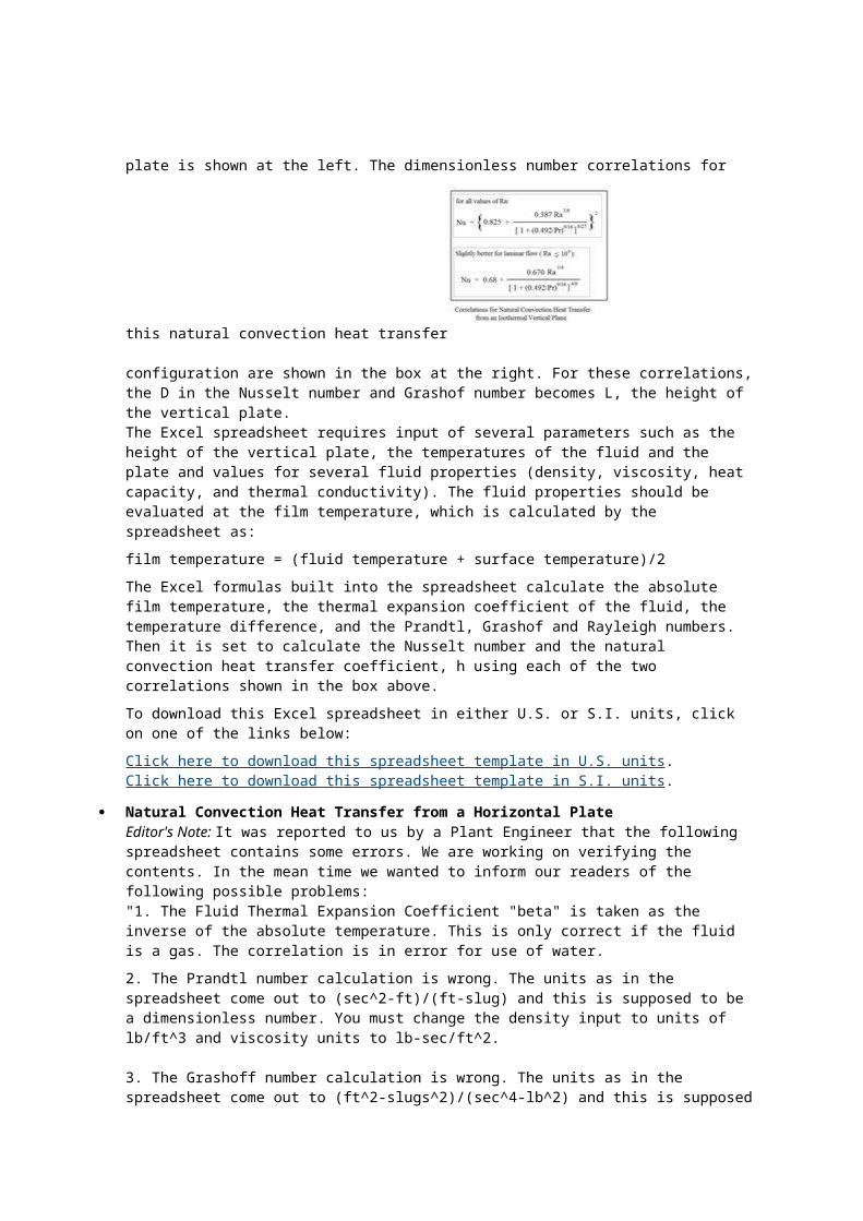
plate is shown at the left. The dimensionless number correlations for

this natural convection heat transfer  

configuration are shown in the box at the right. For these correlations,the D in the Nusselt number and Grashof number becomes L, the height of the vertical plate.The Excel spreadsheet requires input of several parameters such as the height of the vertical plate, the temperatures of the fluid and the plate and values for several fluid properties (density, viscosity, heat capacity, and thermal conductivity). The fluid properties should be evaluated at the film temperature, which is calculated by the spreadsheet as:film temperature = (fluid temperature + surface temperature)/2The Excel formulas built into the spreadsheet calculate the absolute film temperature, the thermal expansion coefficient of the fluid, the temperature difference, and the Prandtl, Grashof and Rayleigh numbers. Then it is set to calculate the Nusselt number and the natural convection heat transfer coefficient, h using each of the two correlations shown in the box above.To download this Excel spreadsheet in either U.S. or S.I. units, click on one of the links below:Click here to download this spreadsheet template in U.S. units.Click here to download this spreadsheet template in S.I. units.

Natural Convection Heat Transfer from a Horizontal PlateEditor's Note: It was reported to us by a Plant Engineer that the following spreadsheet contains some errors. We are working on verifying the contents. In the mean time we wanted to inform our readers of the following possible problems:"1. The Fluid Thermal Expansion Coefficient "beta" is taken as the inverse of the absolute temperature. This is only correct if the fluid is a gas. The correlation is in error for use of water.2. The Prandtl number calculation is wrong. The units as in the spreadsheet come out to (sec^2-ft)/(ft-slug) and this is supposed to be a dimensionless number. You must change the density input to units of lb/ft^3 and viscosity units to lb-sec/ft^2. 

3. The Grashoff number calculation is wrong. The units as in the spreadsheet come out to (ft^2-slugs^2)/(sec^4-lb^2) and this is supposed

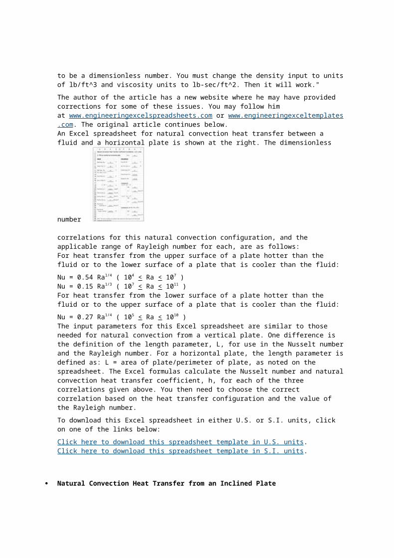
to be a dimensionless number. You must change the density input to unitsof lb/ft^3 and viscosity units to lb-sec/ft^2. Then it will work."The author of the article has a new website where he may have provided corrections for some of these issues. You may follow him at www.engineeringexcelspreadsheets.com or www.engineeringexceltemplates.com. The original article continues below.An Excel spreadsheet for natural convection heat transfer between a fluid and a horizontal plate is shown at the right. The dimensionless

number  

correlations for this natural convection configuration, and the applicable range of Rayleigh number for each, are as follows:For heat transfer from the upper surface of a plate hotter than the fluid or to the lower surface of a plate that is cooler than the fluid:Nu = 0.54 Ra1/4 ( 104 < Ra < 107 )Nu = 0.15 Ra1/3 ( 107 < Ra < 1011 )For heat transfer from the lower surface of a plate hotter than the fluid or to the upper surface of a plate that is cooler than the fluid:Nu = 0.27 Ra1/4 ( 105 < Ra < 1010 )The input parameters for this Excel spreadsheet are similar to those needed for natural convection from a vertical plate. One difference is the definition of the length parameter, L, for use in the Nusselt numberand the Rayleigh number. For a horizontal plate, the length parameter isdefined as: L = area of plate/perimeter of plate, as noted on the spreadsheet. The Excel formulas calculate the Nusselt number and naturalconvection heat transfer coefficient, h, for each of the three correlations given above. You then need to choose the correct correlation based on the heat transfer configuration and the value of the Rayleigh number.To download this Excel spreadsheet in either U.S. or S.I. units, click on one of the links below:Click here to download this spreadsheet template in U.S. units.Click here to download this spreadsheet template in S.I. units.

Natural Convection Heat Transfer from an Inclined Plate

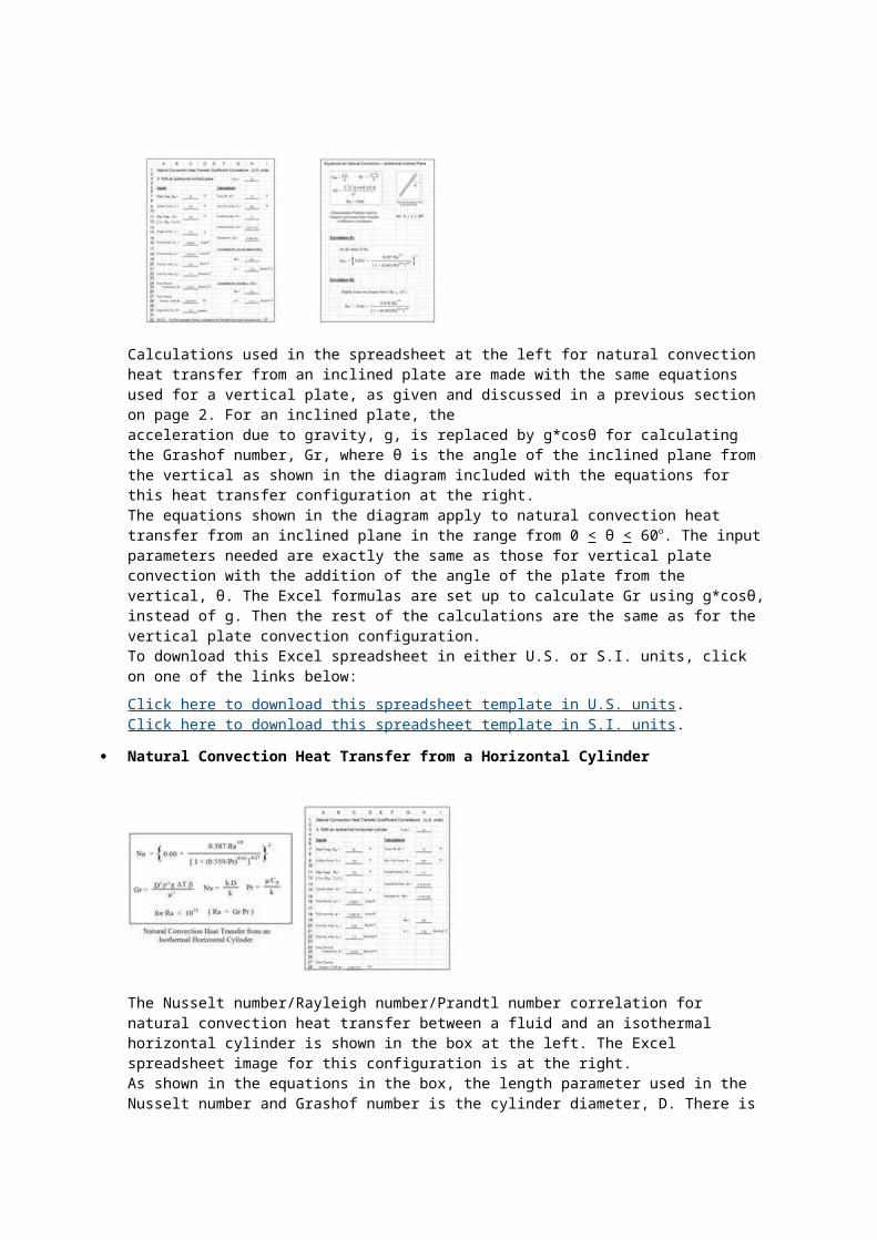
Calculations used in the spreadsheet at the left for natural convection heat transfer from an inclined plate are made with the same equations used for a vertical plate, as given and discussed in a previous section on page 2. For an inclined plate, the acceleration due to gravity, g, is replaced by g*cosθ for calculating the Grashof number, Gr, where θ is the angle of the inclined plane from the vertical as shown in the diagram included with the equations for this heat transfer configuration at the right.The equations shown in the diagram apply to natural convection heat transfer from an inclined plane in the range from 0 < θ < 60o. The input parameters needed are exactly the same as those for vertical plate convection with the addition of the angle of the plate from the vertical, θ. The Excel formulas are set up to calculate Gr using g*cosθ,instead of g. Then the rest of the calculations are the same as for the vertical plate convection configuration.To download this Excel spreadsheet in either U.S. or S.I. units, click on one of the links below:Click here to download this spreadsheet template in U.S. units.Click here to download this spreadsheet template in S.I. units.

Natural Convection Heat Transfer from a Horizontal Cylinder

The Nusselt number/Rayleigh number/Prandtl number correlation for natural convection heat transfer between a fluid and an isothermal horizontal cylinder is shown in the box at the left. The Excel spreadsheet image for this configuration is at the right.As shown in the equations in the box, the length parameter used in the Nusselt number and Grashof number is the cylinder diameter, D. There is

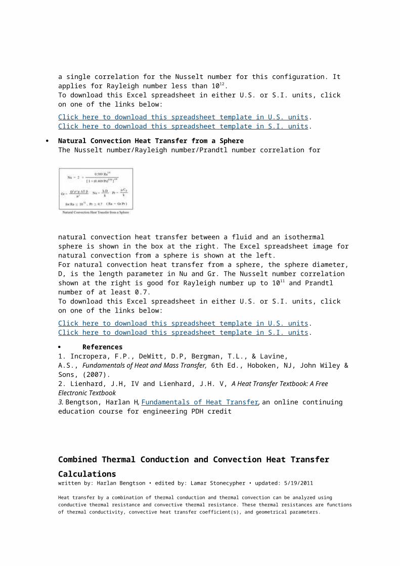
a single correlation for the Nusselt number for this configuration. It applies for Rayleigh number less than 1012.To download this Excel spreadsheet in either U.S. or S.I. units, click on one of the links below:Click here to download this spreadsheet template in U.S. units.Click here to download this spreadsheet template in S.I. units.

Natural Convection Heat Transfer from a SphereThe Nusselt number/Rayleigh number/Prandtl number correlation for

 natural convection heat transfer between a fluid and an isothermal sphere is shown in the box at the right. The Excel spreadsheet image fornatural convection from a sphere is shown at the left.For natural convection heat transfer from a sphere, the sphere diameter,D, is the length parameter in Nu and Gr. The Nusselt number correlation shown at the right is good for Rayleigh number up to 1011 and Prandtl number of at least 0.7.To download this Excel spreadsheet in either U.S. or S.I. units, click on one of the links below:Click here to download this spreadsheet template in U.S. units.Click here to download this spreadsheet template in S.I. units.

References1. Incropera, F.P., DeWitt, D.P, Bergman, T.L., & Lavine, A.S., Fundamentals of Heat and Mass Transfer, 6th Ed., Hoboken, NJ, John Wiley &Sons, (2007).2. Lienhard, J.H, IV and Lienhard, J.H. V, A Heat Transfer Textbook: A Free Electronic Textbook3. Bengtson, Harlan H, Fundamentals of Heat Transfer, an online continuing education course for engineering PDH credit

Combined Thermal Conduction and Convection Heat Transfer Calculationswritten by: Harlan Bengtson • edited by: Lamar Stonecypher • updated: 5/19/2011

Heat transfer by a combination of thermal conduction and thermal convection can be analyzed using conductive thermal resistance and convective thermal resistance. These thermal resistances are functionsof thermal conductivity, convective heat transfer coefficient(s), and geometrical parameters.

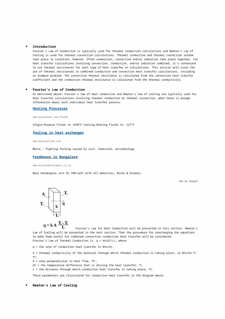
IntroductionFourier's Law of Conduction is typically used for thermal conduction calculations and Newton's Law of Cooling is used for thermal convection calculations. Thermal conduction and thermal convection seldom take place in isolation, however. Often conduction, convection and/or radiation take place together. Forheat transfer calculations involving convection, conduction, and/or radiation combined, it's convenient to use thermal resistances for each type of heat transfer in calculations. This article will cover the use of thermal resistances in combined conduction and convection heat transfer calculations, including an example problem. The convection thermal resistance is calculated from the convection heat transfer coefficient and the conduction thermal resistance is calculated from the thermal conductivity.

Fourier's Law of ConductionAs mentioned above, Fourier's law of heat conduction and Newton's law of cooling are typically used for heat transfer calculations involving thermal conduction or thermal convection, when there is enough information about each individual heat transfer process.

Heating Processes

www.paratherm.com/fluids

Single-Purpose Fluids to +650°F Cooling-Heating Fluids to -127°F

fouling in heat exchanger

www.merusonline.com

Merus - fighting fouling caused by rust, limescale, microbiology

Farmhouse in Bangalore

www.divinedevelopers.co.in

Near Kanakapura Just Rs.188/sqft with all amenities, Birds & Animals

Ads by Google

Fourier's Law for Heat Conduction will be presented in this section. Newton'sLaw of Cooling will be presented in the next section. Then the procedure for rearranging the equations to make them useful for combined convection conduction heat transfer will be considered.Fourier's Law of Thermal Conduction is: q = kA(ΔT/L), where

q = the rate of conduction heat transfer in Btu/hr,

k = thermal conductivity of the material through which thermal conduction is taking place, in Btu/hr-oF-ft,A = area perpendicular to heat flow, ft2,ΔT = the temperature difference that is driving the heat transfer, oF,L = the distance through which conduction heat transfer is taking place, ft.

These parameters are illustrated for conduction heat transfer in the diagram above.

Newton's Law of Cooling

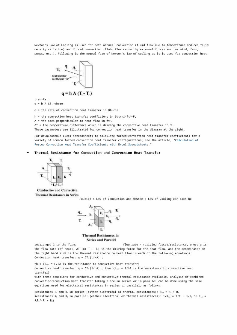
Newton's Law of Cooling is used for both natural convection (fluid flow due to temperature induced fluiddensity variation) and forced convection (fluid flow caused by external forces such as wind, fans, pumps, etc.). Following is the normal form of Newton's law of cooling as it is used for convection heat

transfer:q = h A ΔT, where

q = the rate of convection heat transfer in Btu/hr,

h = the convection heat transfer coefficient in But/hr-ft2-oF,A = the area perpendicular to heat flow in ft2,ΔT = the temperature difference which is driving the convective heat transfer in oF.These parameters are illustrated for convection heat transfer in the diagram at the right.

For downloadable Excel spreadsheets to calculate forced convection heat transfer coefficients for a variety of common forced convection heat transfer configurations, see the article, "Calculation of Forced Convection Heat Transfer Coefficients with Excel Spreadsheets."

Thermal Resistance for Conduction and Convection Heat Transfer

Fourier's Law of Conduction and Newton's Law of Cooling can each be

rearranged into the form:  flow rate = (driving force)/resistance, where q is the flow rate (of heat), ΔT (or T1 - T2) is the driving force for the heat flow, and the denominator on the right hand side is the thermal resistance to heat flow in each of the following equations:Conduction heat transfer: q = ΔT/(L/kA) ;

thus {Rcond = L/kA is the resistance to conductive heat transfer}Convective heat transfer: q = ΔT/(1/hA) ; thus {Rconv = 1/hA is the resistance to convective heat transfer}With these equations for conductive and convective thermal resistance available, analysis of combined convection/conduction heat transfer taking place in series or in parallel can be done using the same equations used for electrical resistances in series or parallel, as follows:

Resistances R1 and R2 in series (either electrical or thermal resistances): Rtot = R1 + R2

Resistances R1 and R2 in parallel (either electrical or thermal resistances): 1/Rtot = 1/R1 + 1/R2 or Rtot = R1R2/(R1 + R2)

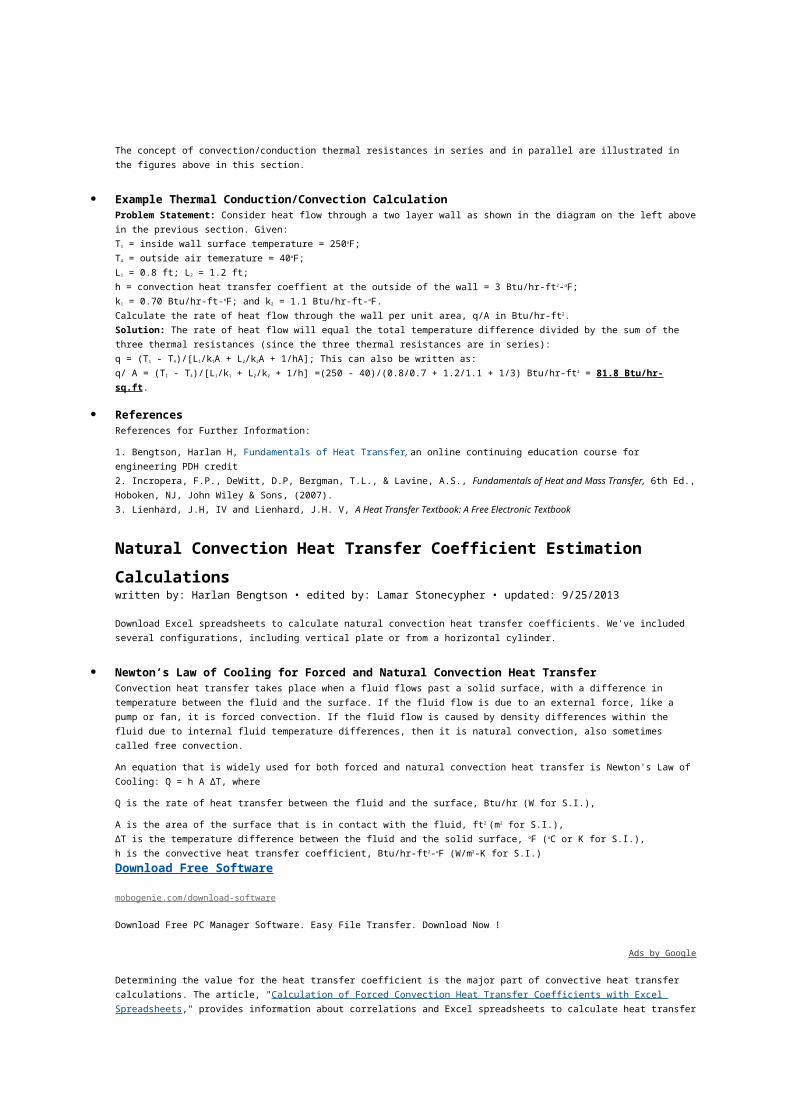
The concept of convection/conduction thermal resistances in series and in parallel are illustrated in the figures above in this section.

Example Thermal Conduction/Convection CalculationProblem Statement: Consider heat flow through a two layer wall as shown in the diagram on the left abovein the previous section. Given:T1 = inside wall surface temperature = 250oF;T4 = outside air temerature = 40oF;L1 = 0.8 ft; L2 = 1.2 ft;h = convection heat transfer coeffient at the outside of the wall = 3 Btu/hr-ft2-oF;k1 = 0.70 Btu/hr-ft-oF; and k2 = 1.1 Btu/hr-ft-oF.Calculate the rate of heat flow through the wall per unit area, q/A in Btu/hr-ft2.Solution: The rate of heat flow will equal the total temperature difference divided by the sum of the three thermal resistances (since the three thermal resistances are in series):q = (T1 - T4)/[L1/k1A + L2/k2A + 1/hA]; This can also be written as:q/ A = (T1 - T4)/[L1/k1 + L2/k2 + 1/h] =(250 - 40)/(0.8/0.7 + 1.2/1.1 + 1/3) Btu/hr-ft2 = 81.8 Btu/hr-sq.ft.

ReferencesReferences for Further Information:

1. Bengtson, Harlan H, Fundamentals of Heat Transfer, an online continuing education course for engineering PDH credit2. Incropera, F.P., DeWitt, D.P, Bergman, T.L., & Lavine, A.S., Fundamentals of Heat and Mass Transfer, 6th Ed.,Hoboken, NJ, John Wiley & Sons, (2007).3. Lienhard, J.H, IV and Lienhard, J.H. V, A Heat Transfer Textbook: A Free Electronic Textbook

Natural Convection Heat Transfer Coefficient Estimation Calculationswritten by: Harlan Bengtson • edited by: Lamar Stonecypher • updated: 9/25/2013

Download Excel spreadsheets to calculate natural convection heat transfer coefficients. We've included several configurations, including vertical plate or from a horizontal cylinder.

Newton’s Law of Cooling for Forced and Natural Convection Heat TransferConvection heat transfer takes place when a fluid flows past a solid surface, with a difference in temperature between the fluid and the surface. If the fluid flow is due to an external force, like a pump or fan, it is forced convection. If the fluid flow is caused by density differences within the fluid due to internal fluid temperature differences, then it is natural convection, also sometimes called free convection.

An equation that is widely used for both forced and natural convection heat transfer is Newton's Law of Cooling: Q = h A ΔT, where

Q is the rate of heat transfer between the fluid and the surface, Btu/hr (W for S.I.),

A is the area of the surface that is in contact with the fluid, ft2 (m2 for S.I.),ΔT is the temperature difference between the fluid and the solid surface, oF (oC or K for S.I.),h is the convective heat transfer coefficient, Btu/hr-ft2-oF (W/m2-K for S.I.)Download Free Software

mobogenie.com/download-software

Download Free PC Manager Software. Easy File Transfer. Download Now !

Ads by Google

Determining the value for the heat transfer coefficient is the major part of convective heat transfer calculations. The article, "Calculation of Forced Convection Heat Transfer Coefficients with Excel Spreadsheets," provides information about correlations and Excel spreadsheets to calculate heat transfer

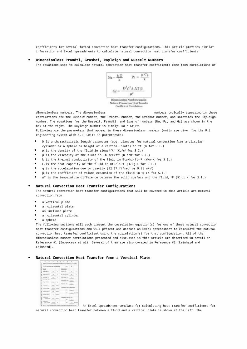
coefficients for several forced convection heat transfer configurations. This article provides similar information and Excel spreadsheets to calculate natural convection heat transfer coefficients.

Dimensionless Prandtl, Grashof, Rayleigh and Nusselt NumbersThe equations used to calculate natural convection heat transfer coefficients come from correlations of

dimensionless numbers. The dimensionless  numbers typically appearing in thesecorrelations are the Nusselt number, the Prandtl number, the Grashof number, and sometimes the Rayleigh number. The equations for the Nusselt, Prandtl, and Grashof numbers (Nu, Pr, and Gr) are shown in the box at the right. The Rayleigh number is simply: Ra = Gr Pr.Following are the parameters that appear in these dimensionless numbers (units are given for the U.S engineering system with S.I. units in parentheses):

D is a characteristic length parameter (e.g. diameter for natural convection from a circular cylinder or a sphere or height of a vertical plate) in ft (m for S.I.)

ρ is the density of the fluid in slugs/ft3 (Kg/m3 for S.I.) μ is the viscosity of the fluid in lb-sec/ft2 (N-s/m2 for S.I.) k is the thermal conductivity of the fluid in Btu/hr-ft-oF (W/m-K for S.I.) Cp is the heat capacity of the fluid in Btu/lb-oF (J/kg-K for S.I.) g is the acceleration due to gravity (32.17 ft/sec2 or 9.81 m/s2) β is the coefficient of volume expansion of the fluid in oR (K for S.I.) ΔT is the temperature difference between the solid surface and the fluid, oF (oC or K for S.I.)

Natural Convection Heat Transfer ConfigurationsThe natural convection heat transfer configurations that will be covered in this article are natural convection from:

a vertical plate a horizontal plate an inclined plate a horizontal cylinder a sphereThe following sections will each present the correlation equation(s) for one of these natural convectionheat transfer configurations and will present and discuss an Excel spreadsheet to calculate the natural convection heat transfer coefficient using the correlation(s) for that configuration. All of the dimensionless number correlations presented and discussed in this article are described in detail in Reference #1 (Inprocera et al). Several of them are also covered in Reference #2 (Leinhard and Leinhard).

Natural Convection Heat Transfer from a Vertical Plate

An Excel spreadsheet template for calculating heat transfer coefficients for natural convection heat transfer between a fluid and a vertical plate is shown at the left. The

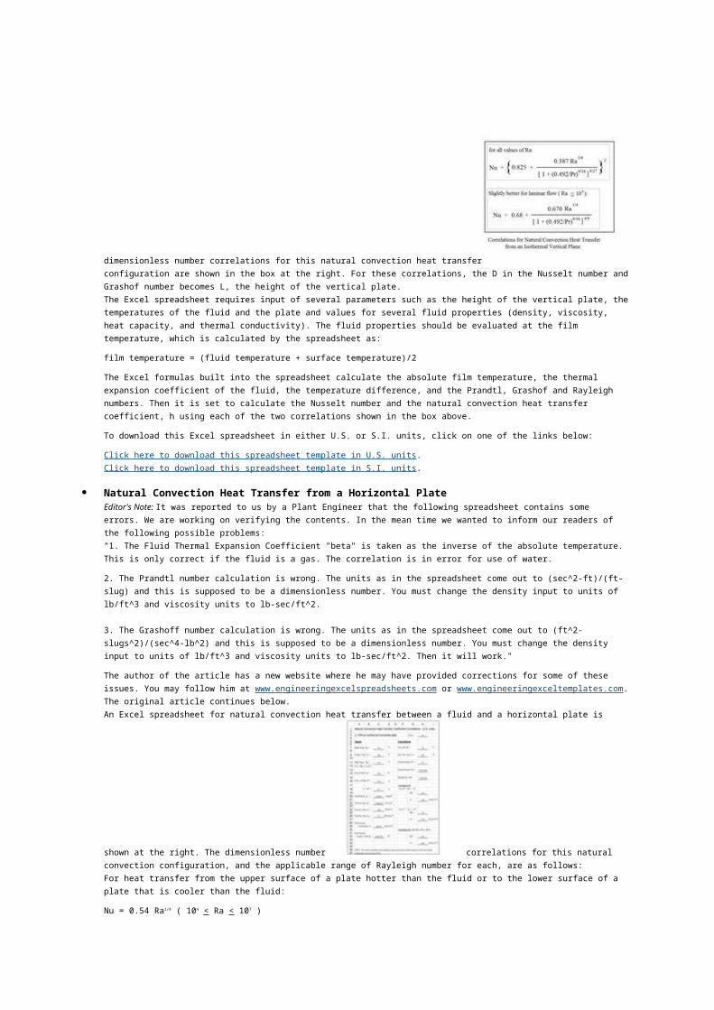
dimensionless number correlations for this natural convection heat transfer  configuration are shown in the box at the right. For these correlations, the D in the Nusselt number andGrashof number becomes L, the height of the vertical plate.The Excel spreadsheet requires input of several parameters such as the height of the vertical plate, thetemperatures of the fluid and the plate and values for several fluid properties (density, viscosity, heat capacity, and thermal conductivity). The fluid properties should be evaluated at the film temperature, which is calculated by the spreadsheet as:

film temperature = (fluid temperature + surface temperature)/2

The Excel formulas built into the spreadsheet calculate the absolute film temperature, the thermal expansion coefficient of the fluid, the temperature difference, and the Prandtl, Grashof and Rayleigh numbers. Then it is set to calculate the Nusselt number and the natural convection heat transfer coefficient, h using each of the two correlations shown in the box above.

To download this Excel spreadsheet in either U.S. or S.I. units, click on one of the links below:

Click here to download this spreadsheet template in U.S. units.Click here to download this spreadsheet template in S.I. units.

Natural Convection Heat Transfer from a Horizontal PlateEditor's Note: It was reported to us by a Plant Engineer that the following spreadsheet contains some errors. We are working on verifying the contents. In the mean time we wanted to inform our readers of the following possible problems:"1. The Fluid Thermal Expansion Coefficient "beta" is taken as the inverse of the absolute temperature. This is only correct if the fluid is a gas. The correlation is in error for use of water.

2. The Prandtl number calculation is wrong. The units as in the spreadsheet come out to (sec^2-ft)/(ft-slug) and this is supposed to be a dimensionless number. You must change the density input to units of lb/ft^3 and viscosity units to lb-sec/ft^2. 

3. The Grashoff number calculation is wrong. The units as in the spreadsheet come out to (ft^2-slugs^2)/(sec^4-lb^2) and this is supposed to be a dimensionless number. You must change the density input to units of lb/ft^3 and viscosity units to lb-sec/ft^2. Then it will work."

The author of the article has a new website where he may have provided corrections for some of these issues. You may follow him at www.engineeringexcelspreadsheets.com or www.engineeringexceltemplates.com.The original article continues below.An Excel spreadsheet for natural convection heat transfer between a fluid and a horizontal plate is

shown at the right. The dimensionless number  correlations for this natural convection configuration, and the applicable range of Rayleigh number for each, are as follows:For heat transfer from the upper surface of a plate hotter than the fluid or to the lower surface of a plate that is cooler than the fluid:

Nu = 0.54 Ra1/4 ( 104 < Ra < 107 )

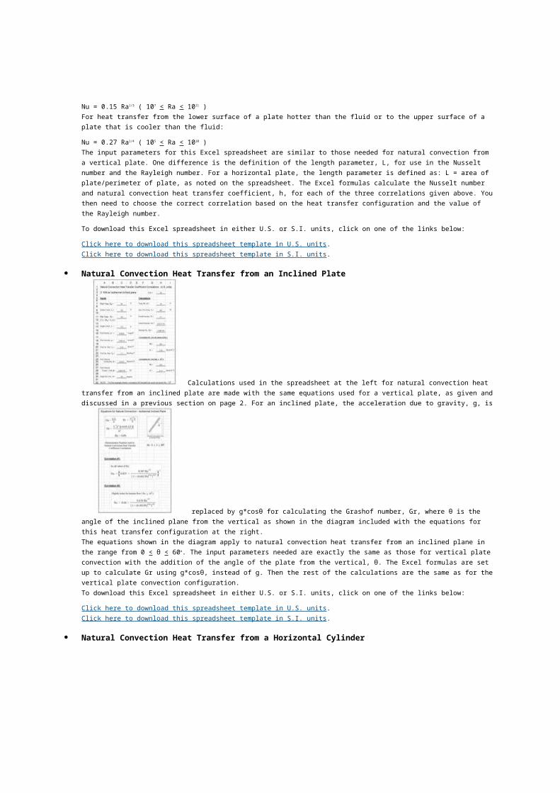
Nu = 0.15 Ra1/3 ( 107 < Ra < 1011 )For heat transfer from the lower surface of a plate hotter than the fluid or to the upper surface of a plate that is cooler than the fluid:

Nu = 0.27 Ra1/4 ( 105 < Ra < 1010 )The input parameters for this Excel spreadsheet are similar to those needed for natural convection from a vertical plate. One difference is the definition of the length parameter, L, for use in the Nusselt number and the Rayleigh number. For a horizontal plate, the length parameter is defined as: L = area of plate/perimeter of plate, as noted on the spreadsheet. The Excel formulas calculate the Nusselt number and natural convection heat transfer coefficient, h, for each of the three correlations given above. Youthen need to choose the correct correlation based on the heat transfer configuration and the value of the Rayleigh number.

To download this Excel spreadsheet in either U.S. or S.I. units, click on one of the links below:

Click here to download this spreadsheet template in U.S. units.Click here to download this spreadsheet template in S.I. units.

Natural Convection Heat Transfer from an Inclined Plate

Calculations used in the spreadsheet at the left for natural convection heat transfer from an inclined plate are made with the same equations used for a vertical plate, as given anddiscussed in a previous section on page 2. For an inclined plate, the acceleration due to gravity, g, is

 replaced by g*cosθ for calculating the Grashof number, Gr, where θ is the angle of the inclined plane from the vertical as shown in the diagram included with the equations for this heat transfer configuration at the right.The equations shown in the diagram apply to natural convection heat transfer from an inclined plane in the range from 0 < θ < 60o. The input parameters needed are exactly the same as those for vertical plateconvection with the addition of the angle of the plate from the vertical, θ. The Excel formulas are set up to calculate Gr using g*cosθ, instead of g. Then the rest of the calculations are the same as for thevertical plate convection configuration.To download this Excel spreadsheet in either U.S. or S.I. units, click on one of the links below:

Click here to download this spreadsheet template in U.S. units.Click here to download this spreadsheet template in S.I. units.

Natural Convection Heat Transfer from a Horizontal Cylinder

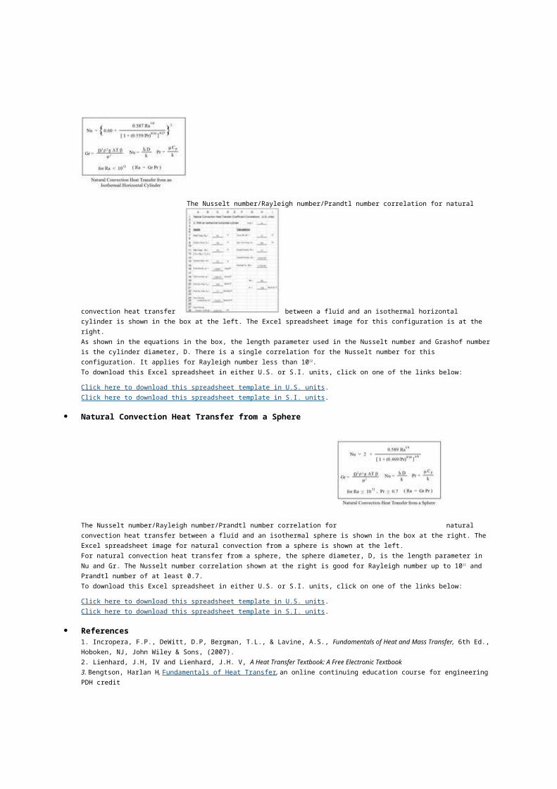
The Nusselt number/Rayleigh number/Prandtl number correlation for natural

convection heat transfer  between a fluid and an isothermal horizontal cylinder is shown in the box at the left. The Excel spreadsheet image for this configuration is at the right.As shown in the equations in the box, the length parameter used in the Nusselt number and Grashof numberis the cylinder diameter, D. There is a single correlation for the Nusselt number for this configuration. It applies for Rayleigh number less than 1012.To download this Excel spreadsheet in either U.S. or S.I. units, click on one of the links below:

Click here to download this spreadsheet template in U.S. units.Click here to download this spreadsheet template in S.I. units.

Natural Convection Heat Transfer from a Sphere

The Nusselt number/Rayleigh number/Prandtl number correlation for  natural convection heat transfer between a fluid and an isothermal sphere is shown in the box at the right. The Excel spreadsheet image for natural convection from a sphere is shown at the left.For natural convection heat transfer from a sphere, the sphere diameter, D, is the length parameter in Nu and Gr. The Nusselt number correlation shown at the right is good for Rayleigh number up to 1011 and Prandtl number of at least 0.7.To download this Excel spreadsheet in either U.S. or S.I. units, click on one of the links below:

Click here to download this spreadsheet template in U.S. units.Click here to download this spreadsheet template in S.I. units.

References1. Incropera, F.P., DeWitt, D.P, Bergman, T.L., & Lavine, A.S., Fundamentals of Heat and Mass Transfer, 6th Ed.,Hoboken, NJ, John Wiley & Sons, (2007).2. Lienhard, J.H, IV and Lienhard, J.H. V, A Heat Transfer Textbook: A Free Electronic Textbook3. Bengtson, Harlan H, Fundamentals of Heat Transfer, an online continuing education course for engineeringPDH credit

Calculation of Forced Convection Heat Transfer Coefficientswritten by: Harlan Bengtson • edited by: Lamar Stonecypher • updated: 5/8/2013

Forced convection heat transfer coefficient correlations are in terms of Nusselt, Prandtl, and Reynolds numbers. Download Excel spreadsheets to help calculate coefficients for several common forced convectionheat transfer configurations.

BackgroundForced convection heat transfer takes place between a solid surface and a fluid that is moving past it. The equation typically used for forced convection heat transfer calculations is Newton's Law of Cooling:Q = h A ΔT, where

Q is the rate of heat transfer between the surface and the fluid in Btu/hr (W for S.I.),

A is the area of the surface in contact with the fluid in ft2 (m2 for S.I.),ΔT is the temperature difference between the solid surface and the fluid in oF (oC or K for S.I.),h is the convective heat transfer coefficient in Btu/hr-ft2-oF (W/m2-K for S.I.)The biggest part of forced convection heat transfer calculations is determination of a value for the convective heat transfer coefficient, h, for the heat transfer configuration of interest. Empirical correlations are available for common forced convection configurations, such as flow through a circular pipe, external flow around a cylinder or a bank of cylinders, and flow through an annulus. These empirical correlations are usually in terms of the dimensionless numbers discussed in the next section. The rest of the article is devoted to presentation and discussion of correlations for several forced convection heat transfer configurations with downloadable Excel spreadsheets for each.

Heat transfer

www.hotscreen.se

All purpose heat transfer Best prices in europe!

Download Free Software

mobogenie.com/download-software

Download Free PC Manager Software. Easy File Transfer. Download Now !

Sap Excel Download

www.smartexporter.de/en

Export data from SAP® and analyze tax-relevant data. Quickly & easily

Ads by Google

Dimensionless Nusselt, Reynolds, and Prandtl Numbers

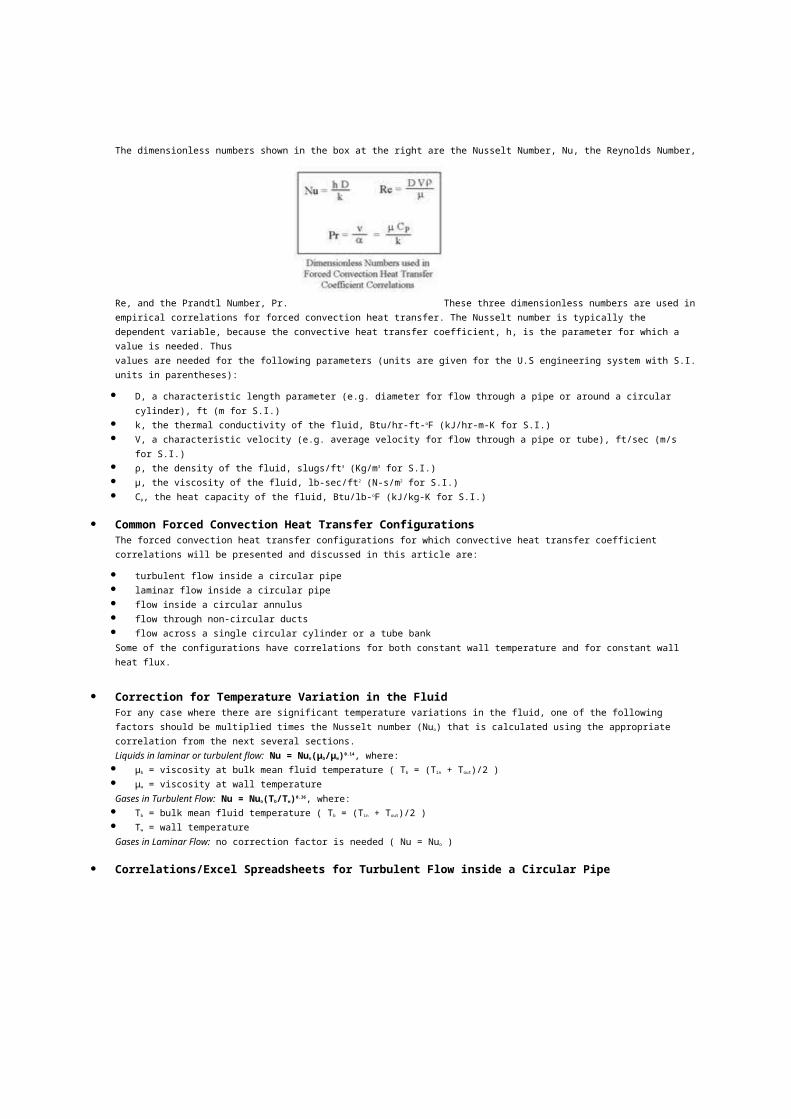
The dimensionless numbers shown in the box at the right are the Nusselt Number, Nu, the Reynolds Number,

Re, and the Prandtl Number, Pr.  These three dimensionless numbers are used inempirical correlations for forced convection heat transfer. The Nusselt number is typically the dependent variable, because the convective heat transfer coefficient, h, is the parameter for which a value is needed. Thusvalues are needed for the following parameters (units are given for the U.S engineering system with S.I.units in parentheses):

D, a characteristic length parameter (e.g. diameter for flow through a pipe or around a circular cylinder), ft (m for S.I.)

k, the thermal conductivity of the fluid, Btu/hr-ft-oF (kJ/hr-m-K for S.I.) V, a characteristic velocity (e.g. average velocity for flow through a pipe or tube), ft/sec (m/s

for S.I.) ρ, the density of the fluid, slugs/ft3 (Kg/m3 for S.I.) μ, the viscosity of the fluid, lb-sec/ft2 (N-s/m2 for S.I.) Cp, the heat capacity of the fluid, Btu/lb-oF (kJ/kg-K for S.I.)

Common Forced Convection Heat Transfer ConfigurationsThe forced convection heat transfer configurations for which convective heat transfer coefficient correlations will be presented and discussed in this article are:

turbulent flow inside a circular pipe laminar flow inside a circular pipe flow inside a circular annulus flow through non-circular ducts flow across a single circular cylinder or a tube bankSome of the configurations have correlations for both constant wall temperature and for constant wall heat flux.

Correction for Temperature Variation in the FluidFor any case where there are significant temperature variations in the fluid, one of the following factors should be multiplied times the Nusselt number (Nuo) that is calculated using the appropriate correlation from the next several sections.Liquids in laminar or turbulent flow: Nu = Nuo(μb/μw)0.14, where: μb = viscosity at bulk mean fluid temperature ( Tb = (Tin + Tout)/2 ) μw = viscosity at wall temperatureGases in Turbulent Flow: Nu = Nuo(Tb/Tw)0.36, where: Tb = bulk mean fluid temperature ( Tb = (Tin + Tout)/2 ) Tw = wall temperatureGases in Laminar Flow: no correction factor is needed ( Nu = Nuo )

Correlations/Excel Spreadsheets for Turbulent Flow inside a Circular Pipe

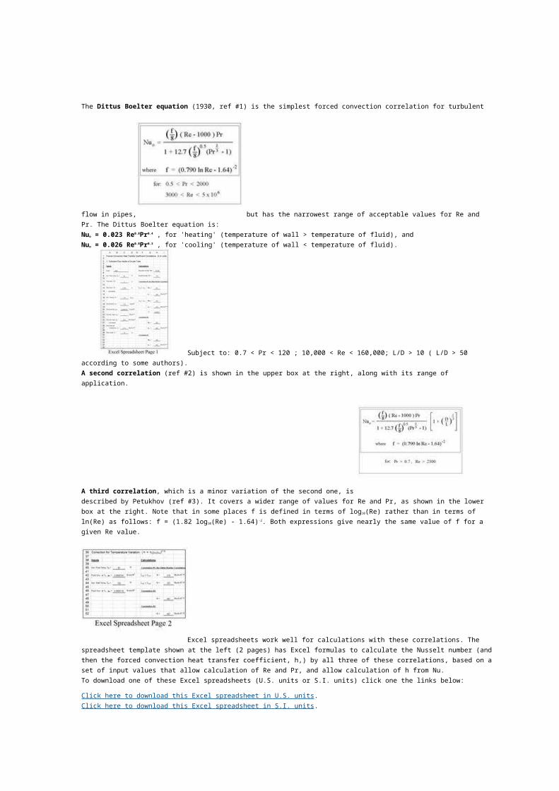
The Dittus Boelter equation (1930, ref #1) is the simplest forced convection correlation for turbulent

flow in pipes,  but has the narrowest range of acceptable values for Re and Pr. The Dittus Boelter equation is:Nuo = 0.023 Re0.8Pr0.4 , for 'heating' (temperature of wall > temperature of fluid), andNuo = 0.026 Re0.8Pr0.3 , for 'cooling' (temperature of wall < temperature of fluid).

Subject to: 0.7 < Pr < 120 ; 10,000 < Re < 160,000; L/D > 10 ( L/D > 50 according to some authors).A second correlation (ref #2) is shown in the upper box at the right, along with its range of application.

A third correlation, which is a minor variation of the second one, is described by Petukhov (ref #3). It covers a wider range of values for Re and Pr, as shown in the lower box at the right. Note that in some places f is defined in terms of log10(Re) rather than in terms of ln(Re) as follows: f = (1.82 log10(Re) - 1.64)-2. Both expressions give nearly the same value of f for a given Re value.

Excel spreadsheets work well for calculations with these correlations. The spreadsheet template shown at the left (2 pages) has Excel formulas to calculate the Nusselt number (andthen the forced convection heat transfer coefficient, h,) by all three of these correlations, based on aset of input values that allow calculation of Re and Pr, and allow calculation of h from Nu.To download one of these Excel spreadsheets (U.S. units or S.I. units) click one the links below:

Click here to download this Excel spreadsheet in U.S. units.Click here to download this Excel spreadsheet in S.I. units.

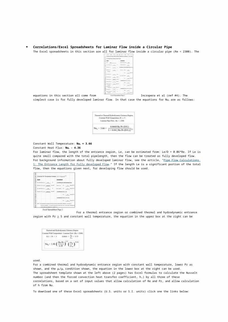
Correlations/Excel Spreadsheets for Laminar Flow inside a Circular PipeThe Excel spreadsheets in this section are all for laminar flow inside a circular pipe (Re < 2300). The

equations in this section all come from  Incropera et al (ref #4). The simplest case is for fully developed laminar flow. In that case the equations for Nuo are as follows:

Constant Wall Temperature: Nuo = 3.66Constant Heat Flux: Nuo - 4.36For laminar flow, the length of the entrance region, Le, can be estimated from: Le/D = 0.06*Re. If Le isquite small compared with the total pipelength, then the flow can be treated as fully developed flow. For background information about fully developed laminar flow, see the article, "Pipe Flow Calculations 1: The Entrance Length for Fully developed Flow." If the length Le is a significant portion of the totalflow, then the equations given next, for developing flow should be used.

For a thermal entrance region or combined thermal and hydrodynamic entrance region with Pr > 5 and constant wall temperature, the equation in the upper box at the right can be

used.For a combined thermal and hydrodynamic entrance region with constant wall temperature, lower Pr as shown, and the μb/μw condition shown, the equation in the lower box at the right can be used.The spreadsheet template shown at the left above (2 pages) has Excel formulas to calculate the Nusselt number (and then the forced convection heat transfer coefficient, h,) by all three of these correlations, based on a set of input values that allow calculation of Re and Pr, and allow calculation of h from Nu.

To download one of these Excel spreadsheets (U.S. units or S.I. units) click one the links below:

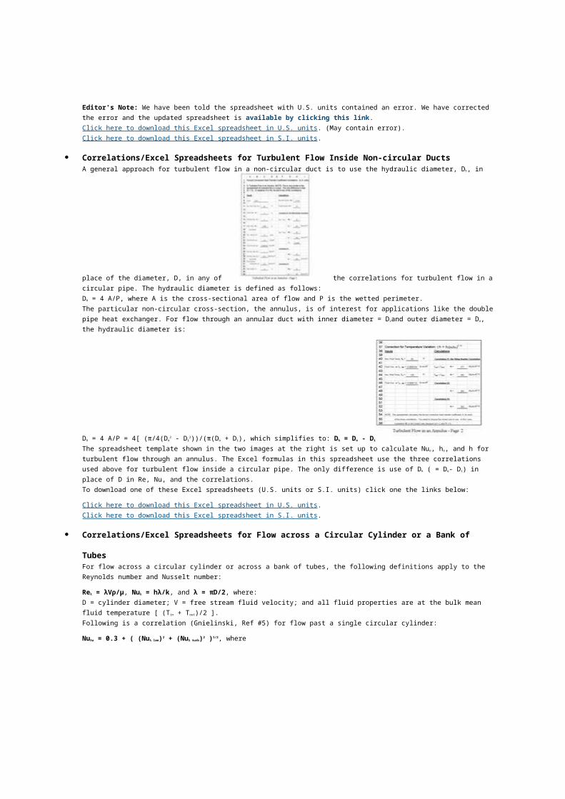
Editor's Note: We have been told the spreadsheet with U.S. units contained an error. We have corrected the error and the updated spreadsheet is available by clicking this link.Click here to download this Excel spreadsheet in U.S. units. (May contain error).Click here to download this Excel spreadsheet in S.I. units.

Correlations/Excel Spreadsheets for Turbulent Flow Inside Non-circular DuctsA general approach for turbulent flow in a non-circular duct is to use the hydraulic diameter, Dh, in

place of the diameter, D, in any of  the correlations for turbulent flow in a circular pipe. The hydraulic diameter is defined as follows:Dh = 4 A/P, where A is the cross-sectional area of flow and P is the wetted perimeter.The particular non-circular cross-section, the annulus, is of interest for applications like the double pipe heat exchanger. For flow through an annular duct with inner diameter = Diand outer diameter = Do, the hydraulic diameter is:

Dh = 4 A/P = 4[ (π/4(Do2 - Di

2))/(π(Do + Di), which simplifies to: Dh = Do - Di

The spreadsheet template shown in the two images at the right is set up to calculate Nuo, ho, and h for turbulent flow through an annulus. The Excel formulas in this spreadsheet use the three correlations used above for turbulent flow inside a circular pipe. The only difference is use of Dh ( = Do- Di) in place of D in Re, Nu, and the correlations.To download one of these Excel spreadsheets (U.S. units or S.I. units) click one the links below:

Click here to download this Excel spreadsheet in U.S. units.Click here to download this Excel spreadsheet in S.I. units.

Correlations/Excel Spreadsheets for Flow across a Circular Cylinder or a Bank of

TubesFor flow across a circular cylinder or across a bank of tubes, the following definitions apply to the Reynolds number and Nusselt number:

Reλ = λVρ/μ, Nuλ = hλ/k, and λ = πD/2, where:D = cylinder diameter; V = free stream fluid velocity; and all fluid properties are at the bulk mean fluid temperature [ (Tin + Tout)/2 ].Following is a correlation (Gnielinski, Ref #5) for flow past a single circular cylinder:

Nuλo = 0.3 + ( (Nuλ lam)2 + (Nuλ turb)2 )1/2, where

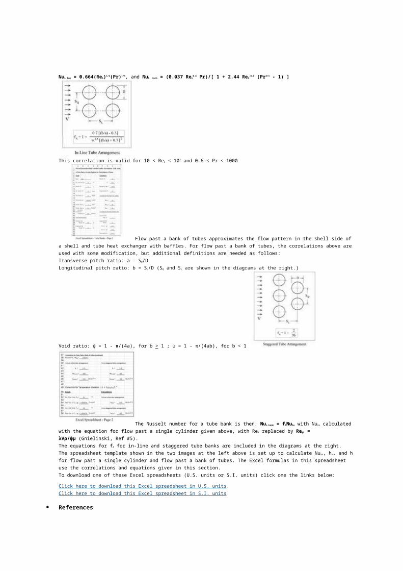
Nuλ lam = 0.664(Reλ)1/2(Pr)1/3, and Nuλ turb = (0.037 Reλ0.8 Pr)/[ 1 + 2.44 Reλ

-0.1 (Pr2/3 - 1) ]

This correlation is valid for 10 < Reλ < 107 and 0.6 < Pr < 1000

Flow past a bank of tubes approximates the flow pattern in the shell side of a shell and tube heat exchanger with baffles. For flow past a bank of tubes, the correlations above are used with some modification, but additional definitions are needed as follows:Transverse pitch ratio: a = SQ/DLongitudinal pitch ratio: b = SL/D (SQ and SL are shown in the diagrams at the right.)

Void ratio: ψ = 1 - π/(4a), for b > 1 ; ψ = 1 - π/(4ab), for b < 1

The Nusselt number for a tube bank is then: Nuo bank = fANuλo with Nuλo calculated with the equation for flow past a single cylinder given above, with Reλ replaced by Reψλ = λVρ/ψμ (Gnielinski, Ref #5).The equations for fA for in-line and staggered tube banks are included in the diagrams at the right.The spreadsheet template shown in the two images at the left above is set up to calculate Nuλo, ho, and hfor flow past a single cylinder and flow past a bank of tubes. The Excel formulas in this spreadsheet use the correlations and equations given in this section.To download one of these Excel spreadsheets (U.S. units or S.I. units) click one the links below:

Click here to download this Excel spreadsheet in U.S. units.Click here to download this Excel spreadsheet in S.I. units.

References

1. Dittus, P.W. and Boelter, L.M., Univ. Calif. Pub. Eng., Vol. 1, No. 13, pp 443-461 (reprinted in Int. Comm. Heat Mass Transfer, Vol. 12, pp 3-22 (1985).2. egr.msu.edu3. Petukhov, B.S., "Heat transfer and friction in turbulent pipe flow with variable physical properties," Adv. Heat Transfer6, 503-565 (1970).4. Incropera, F.P., DeWitt, D.P, Bergman, T.L., & Lavine, A.S., Fundamentals of Heat and Mass Transfer, 6th Ed.,Hoboken, NJ, John Wiley & Sons, (2007).5. Gnielinski, V., "Berechnung mittlerer Warme- und Stoffubergshoeffizienten an laminar und turbulent uberstromten Einzellkorpern mit Hilfe einer einheitlichen Gleichung," Forschung im Ingenierwesen, Vol. 41, pp145-153, (1975). Sample contents.

Fundamentals of Heat Exchanger Theory and Designwritten by: Harlan Bengtson • edited by: Lamar Stonecypher • updated: 10/6/2010

Heat exchanger theory leads to the heat exchanger design equation that relates the overall heat transfercoefficient, heat transfer surface area, and log mean temperature difference to the rate of heat transfer. This heat exchanger design equation is used to find the area needed for heat exchangers.

IntroductionThe heat exchanger design equation can be used to calculate the required heat transfer surface area for a variety of specified fluids, inlet and outlet temperatures and types and configurations of heat exchangers, including counterflow or parallel flow. A value is needed for the overall heat transfer coefficient for the given heat exchanger, fluids, and temperatures. Heat exchanger calculations could bemade for the required heat transfer area, or the rate of heat transfer for a heat exchanger of given area.

The Heat Exchanger Design EquationHeat exchanger theory leads to the basic heat exchanger design equation: Q = U A ΔTlm, whereQ is the rate of heat transfer between the two fluids in the heat exchanger in But/hr,

U is the overall heat transfer coefficient in Btu/hr-ft2-oF,A is the heat transfer surface area in ft2,and ΔTlm is the log mean temperature difference in oF, calculated from the inlet and outlet temperatures of both fluids.heat exchanger pipe

en.tiandapipe.com

China Heat exchanger pipe supplier More accurate&Faster delivery!

Cleaning Heat Exchanger

www.merusonline.com

solution to stop fouling, keep your heat exchanger clean no chemicals

Tube Heat Exchanger

rakshanequipments.net/Enquire_Now

Pioneer Supplier & Manufacturer of Tube Heat Exchanger in Coimbatore.

Ads by Google

For design of heat exchangers, the basic heat exchanger design equation can be used to calculate the required heat exchanger area for known or estimated values of the other three parameters, Q, U, and ΔTlm.Each of those parameters will now be discussed briefly.

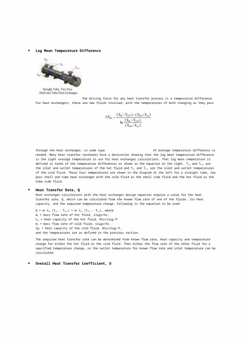
Log Mean Temperature Difference

The driving force for any heat transfer process is a temperature difference. For heat exchangers, there are two fluids involved, with the temperatures of both changing as they pass

through the heat exchanger, so some type  of average temperature difference isneeded. Many heat transfer textbooks have a derivation showing that the log mean temperature difference is the right average temperature to use for heat exchanger calculations. That log mean temperature is defined in terms of the temperature differences as shown in the equation at the right. THin and THout are the inlet and outlet temperatures of the hot fluid and TCin and TCout are the inlet and outlet temperaturesof the cold fluid. Those four temperatures are shown in the diagram at the left for a straight tube, twopass shell and tube heat exchanger with the cold fluid as the shell side fluid and the hot fluid as the tube side fluid.

Heat Transfer Rate, QHeat exchanger calculations with the heat exchanger design equation require a value for the heat transfer rate, Q, which can be calculated from the known flow rate of one of the fluids, its heat capacity, and the required temperature change. Following is the equation to be used:

Q = mH CpH (THin - THout) = mC CpC (TCout - TCin), wheremH = mass flow rate of hot fluid, slugs/hr,CpH = heat capacity of the hot fluid, Btu/slug-oFmC = mass flow rate of cold fluid, slugs/hr,CpC = heat capacity of the cold fluid, Btu/slug-oF,and the temperatures are as defined in the previous section.

The required heat transfer rate can be determined from known flow rate, heat capacity and temperature change for either the hot fluid or the cold fluid. Then either the flow rate of the other fluid for a specified temperature change, or the outlet temperature for known flow rate and inlet temperature can becalculated.

Overall Heat Transfer Coefficient, U

The overall heat transfer coefficient, U, depends on the conductivity through the heat transfer wall

separating the two fluids, and the  convection coefficients on both sides of the heat transfer wall. For a shell and tube heat exchanger, for example, there would be an inside convective coefficient for the tube side fluid and an outside convective coefficient for the shell side fluid. The heat transfer coefficient for a given heat exchanger is often determined empirically by measuring all of the other parameters in the basic heat exchanger equation and calculating U. Typical ranges of U values for various heat exchanger/fluid combinations are available in textbooks, handbooks and on websites. A sampling is given in the table at the right for shell and tube heat exchangers:

SummaryPreliminary heat exchanger design to estimate the required heat exchanger surface area can be done usingthe basic heat exchanger equation, Q = U A ΔTlm, if values are known or can be estimated for Q, U and ΔTlm. Heat exchanger theory tells us that ΔTlm is the right average temperature difference to use.For example preliminary heat exchanger design calculations, see the article, "Preliminary Heat ExchangerDesign Example."For Excel spreadsheet templates that can be downloaded to make preliminary heat exchanger design calculations, see the article: "Excel Spreadsheet Templates for Preliminary Heat Exchanger Design."

References and Image CreditReferences for Further Information:

1. Bengtson, H., Fundamentals of Heat Exchangers, an online, continuing education course for PDH credit2. Kakac, S. and Liu, H., Heat Exchangers: Selection, Rating and Thermal Design, CRC Press, 2002.3. Kuppan, T., Heat Exchanger Design Handbook, CRC Press, 2000.Image Credit:

Straight tube, two pass, shell and tube heat exchanger: http://www.e-steamboilers.com/en/shell_tube_heat_ex.asp

Preliminary Heat Exchanger Design Examplewritten by: Harlan Bengtson • edited by: Lamar Stonecypher • updated: 8/17/2011

Design of heat exchangers is an iterative process, using the heat exchanger design equation to estimate the needed heat transfer area, based on an estimate of the overall heat transfer coefficient, specified heat load, and log mean temperature difference (from inlet and outlet temperatures).

Introduction - The Heat Exchanger Design EquationThe basic heat exchanger design equation,

Q = U A ΔTlm,was introduced and discussed in another article, "Fundamentals of Heat Exchanger Theory and Design." When used as a design equation to calculate the required heat transfer surface area, the equation can berearranged to become:A = Q/(U ΔTlm),where Q is the required heat transfer rate in Btu/hr, U is the overall heat transfer coefficient in Btu/hr-oF, and Δtlm is the log mean temperature difference in oF.

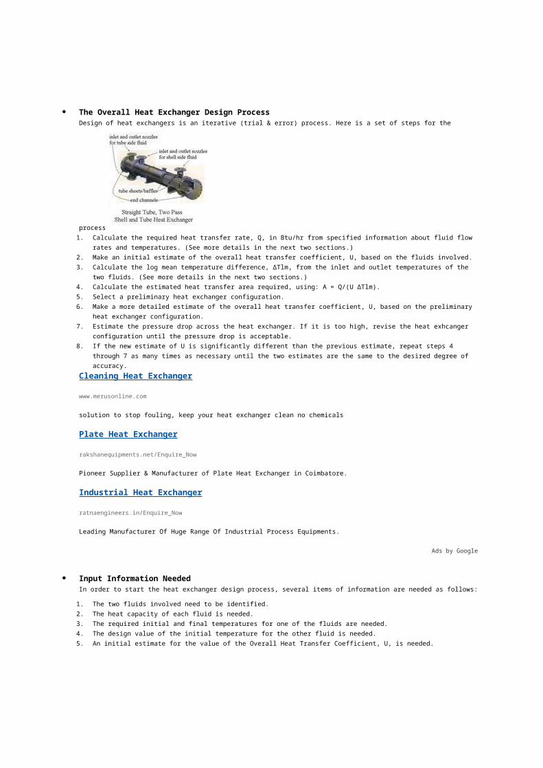
The Overall Heat Exchanger Design ProcessDesign of heat exchangers is an iterative (trial & error) process. Here is a set of steps for the

process1. Calculate the required heat transfer rate, Q, in Btu/hr from specified information about fluid flow

rates and temperatures. (See more details in the next two sections.)2. Make an initial estimate of the overall heat transfer coefficient, U, based on the fluids involved.3. Calculate the log mean temperature difference, ΔTlm, from the inlet and outlet temperatures of the

two fluids. (See more details in the next two sections.)4. Calculate the estimated heat transfer area required, using: A = Q/(U ΔTlm).5. Select a preliminary heat exchanger configuration.6. Make a more detailed estimate of the overall heat transfer coefficient, U, based on the preliminary

heat exchanger configuration.7. Estimate the pressure drop across the heat exchanger. If it is too high, revise the heat exhcanger

configuration until the pressure drop is acceptable.8. If the new estimate of U is significantly different than the previous estimate, repeat steps 4

through 7 as many times as necessary until the two estimates are the same to the desired degree of accuracy.

Cleaning Heat Exchanger

www.merusonline.com

solution to stop fouling, keep your heat exchanger clean no chemicals

Plate Heat Exchanger

rakshanequipments.net/Enquire_Now

Pioneer Supplier & Manufacturer of Plate Heat Exchanger in Coimbatore.

Industrial Heat Exchanger

ratnaengineers.in/Enquire_Now

Leading Manufacturer Of Huge Range Of Industrial Process Equipments.

Ads by Google

Input Information NeededIn order to start the heat exchanger design process, several items of information are needed as follows:

1. The two fluids involved need to be identified.2. The heat capacity of each fluid is needed.3. The required initial and final temperatures for one of the fluids are needed.4. The design value of the initial temperature for the other fluid is needed.5. An initial estimate for the value of the Overall Heat Transfer Coefficient, U, is needed.

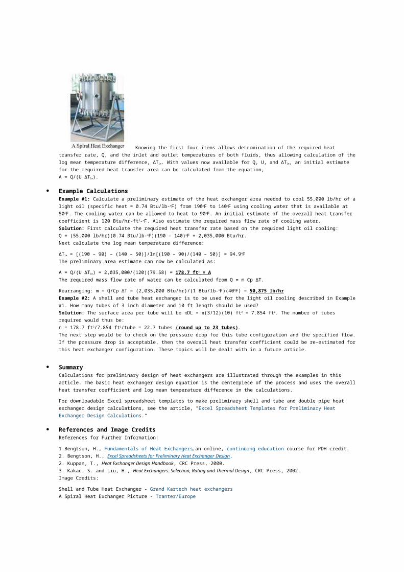
Knowing the first four items allows determination of the required heat transfer rate, Q, and the inlet and outlet temperatures of both fluids, thus allowing calculation of thelog mean temperature difference, ΔTlm. With values now available for Q, U, and ΔTlm, an initial estimate for the required heat transfer area can be calculated from the equation,A = Q/(U ΔTlm).

Example CalculationsExample #1: Calculate a preliminary estimate of the heat exchanger area needed to cool 55,000 lb/hr of alight oil (specific heat = 0.74 Btu/lb-oF) from 190oF to 140oF using cooling water that is available at 50oF. The cooling water can be allowed to heat to 90oF. An initial estimate of the overall heat transfer coefficient is 120 Btu/hr-ft2-oF. Also estimate the required mass flow rate of cooling water.Solution: First calculate the required heat transfer rate based on the required light oil cooling:Q = (55,000 lb/hr)(0.74 Btu/lb-oF)(190 – 140)oF = 2,035,000 Btu/hr.Next calculate the log mean temperature difference:

ΔTlm = [(190 – 90) – (140 – 50)]/ln[(190 – 90)/(140 – 50)] = 94.9oFThe preliminary area estimate can now be calculated as:

A = Q/(U ΔTlm) = 2,035,000/(120)(79.58) = 178.7 ft 2   = A The required mass flow rate of water can be calculated from Q = m Cp ΔT.

Rearranging: m = Q/Cp ΔT = (2,035,000 Btu/hr)/(1 Btu/lb-oF)(40oF) = 50,875 lb/hrExample #2: A shell and tube heat exchanger is to be used for the light oil cooling described in Example#1. How many tubes of 3 inch diameter and 10 ft length should be used?Solution: The surface area per tube will be πDL = π(3/12)(10) ft2 = 7.854 ft2. The number of tubes required would thus be:n = 178.7 ft2/7.854 ft2/tube = 22.7 tubes (round up to 23 tubes).The next step would be to check on the pressure drop for this tube configuration and the specified flow.If the pressure drop is acceptable, then the overall heat transfer coefficient could be re-estimated forthis heat exchanger configuration. These topics will be dealt with in a future article.

SummaryCalculations for preliminary design of heat exchangers are illustrated through the examples in this article. The basic heat exchanger design equation is the centerpiece of the process and uses the overallheat transfer coefficient and log mean temperature difference in the calculations.

For downloadable Excel spreadsheet templates to make preliminary shell and tube and double pipe heat exchanger design calculations, see the article, "Excel Spreadsheet Templates for Preliminary Heat Exchanger Design Calculations."

References and Image CreditsReferences for Further Information:

1.Bengtson, H., Fundamentals of Heat Exchangers, an online, continuing education course for PDH credit.2. Bengtson, H., Excel Spreadsheets for Preliminary Heat Exchanger Design.2. Kuppan, T., Heat Exchanger Design Handbook, CRC Press, 2000.3. Kakac, S. and Liu, H., Heat Exchangers: Selection, Rating and Thermal Design, CRC Press, 2002.Image Credits:

Shell and Tube Heat Exchanger - Grand Kartech heat exchangersA Spiral Heat Exchanger Picture - Tranter/Europe

Preliminary Heat Exchanger Design - Calculations Involvedwritten by: Harlan Bengtson • edited by: Lamar Stonecypher • updated: 10/6/2010

Excel spreadsheet templates for heat exchanger design can be downloaded in either S.I. units or U.S. units. The spreadsheets calculate heat transfer area needed and number of tubes or pipe length, for given values of several variables, including an estimate of the overall heat transfer coefficient.

Equations and ParametersThe heat exchanger design equation, Q = U A ΔTlm, can be used to determine the required heat transfer area, A, for a heat exchanger. The heat transfer area can be calculated after values have been determined or estimated for the required heat transfer rate, Q; the overall heat transfer coefficient, U, and the log mean temperature difference for the heat exchanger, ΔTlm, based on the values of several input parameters. Excel spreadsheet templates for calculating the heat transfer area needed for a heat exchanger are presented and discussed in the next section.For more details about preliminary heat exchanger design, the parameters involved, and example heat exchanger calculations, see the articles: "Preliminary Heat Exchanger Design Example" and "Fundamentals of Heat Exchanger Theory and Design."

Excel Template - Page 1: Calculation of Heat Transfer Area

The Excel spreadsheet template shown at the left will calculate the heat transfer area required for a heat exchanger after values for several parameters have been input. The parameters that need input values are the mass flow rate, specific heat, inlet temperature and outlet temperature of one of the fluids; the heat capacity, inlet temperature and outlet temperature of the second fluid; and an estimated value for the overall heat transfer coefficient. After values are enteredfor those parameters the Excel formulas in the spreadsheet will calculate the heat transfer rate, the log mean temperature difference, the required heat transfer area, and the needed mass flow rate for the second fluid.Plate Heat Exchanger

rakshanequipments.net/Enquire_Now

Pioneer Supplier & Manufacturer of Plate Heat Exchanger in Coimbatore.

Download Free Software

mobogenie.com/download-software

Download Free PC Manager Software. Easy File Transfer. Download Now !

Cleaning Heat Exchanger

www.merusonline.com

solution to stop fouling, keep your heat exchanger clean no chemicals

Ads by Google

Column C has cells for entry of several parameter values. Column I contains the Excel formulas to calculate the parameters noted above. This example spreadsheet shows calculations in U.S. units, howeveran S.I. version and a U.S. version are available for download just below.

Click here to download this Excel spreadsheet template (in U.S. units).Click here to download this Excel spreadsheet template (in S.I. units).

Excel Template - Page 2: Number of Tubes for a Shell and Tube Heat Exchanger

The Excel spreadsheet template at the right is for shell and tube heat

exchanger design. This spreadsheet  calculates the number of tubes needed for a specified tube length and diameter. In the spreadsheet templates that can be downloaded below, this page 2 and page 1 from the previous section are both included as part of the same Excel template. Thus the heat exchange area calculated on page 1 can be used for the page 2 calculations.This example spreadsheet shows calculations in U.S. units, however an S.I. version and a U.S. version are both available for download just below.

Click here to download this Excel spreadsheet template (pages 1 and 2, in U.S. units).Click here to download this Excel spreadsheet template (pages 1 and 2, in S.I. units).For more background information about the different types of shell and tube heat exchangers, see the article: "Types of Shell and Tube Heat Exchangers."

Excel Template- Alternate Page 2 Length of Pipe for a Double Pipe Heat Exchanger

The Excel spreadsheet template at the left is for double pipe heat exchanger

design. This spreadsheet  calculates the length of pipe needed for a double pipe heat exchanger of specified inner pipe diameter and known heat transfer area. The page 1 spreadsheet from the second section in this article is included with this page 2 in the spreadsheet templates that can be downloaded below. The required heat transfer area can thus be taken from the page 1 calculations.This example spreadsheet shows calculations in U.S. units, however an S.I. version and a U.S. version are both available for download just below.

Click here to download this Excel spreadsheet template (pages 1 and 2, in U.S. units).Click here to download this Excel spreadsheet template (pages 1 and 2, in S.I. units).For more background information about double pipe heat exchangers, see the article: "Double Pipe Heat Exchanger Design."

References and Image CreditsReferences for Further Information:

1. Bengtson, H., Fundamentals of Heat Exchangers, an online, continuing education course for PDH credit.2. Kuppan, T., Heat Exchanger Design Handbook, CRC Press, 2000.3. Kakac, S. and Liu, H., Heat Exchangers: Selection, Rating and Thermal Design, CRC Press, 2002.Image Credits:

1. Shell and Tube Heat Exchanger - Grand Kartech heat exchangers2. Double Pipe Heat Exchanger - Chin

Excel Formulas for Pressure Drop in Shell and Tube Heat Exchanger Designwritten by: Harlan Bengtson • edited by: Lamar Stonecypher • updated: 9/28/2011

Excel formulas for calculation of frictional pressure drop in shell and tube and double pipe heat exchanger design can be downloaded from this article. The pressure drop calculation is for the tubes in a shell and tube heat exchanger or for the inside pipe in a double pipe heat exchanger.

Preliminary Heat Exchanger Design Background

Heat exchanger design is a multi-step, iterative process made up of the following steps:

1. Calculate the heat transfer rate, Q, in Btu/hr, based on specified information about fluid flow rates and temperatures.

2. Determine an estimated value for the overall heat transfer coefficient, U, based on the fluids involved.

3. Calculate the log mean temperature difference, ΔTlm, using the inlet and outlet temperatures of the two fluids.

4. Make an initial estimate of the heat transfer area required, using: A = Q/(U ΔTlm).5. Choose a preliminary configuration for the heat exchanger and make necessary calculations (e.g.

number and size of tubes in a shell and tube heat exchanger or pipe diameters and length for a double pipe heat exchanger).

6. Estimate the pressure drop across the heat exchanger. If it is too high or too low, revise the configuration of the heat exchanger until the pressure drop is acceptable.

7. Make a more detailed estimate of the overall heat transfer coefficient, U, based on the current configuration of the heat exchanger.

8. If the latest estimate of U is significantly different than the previous estimate, repeat steps 4 through 7 as many times as necessary until the two estimates are the same to the desired degree of accuracy.

More details about this process are available in the first two articles of this series, "Fundamentals ofHeat Exchanger Theory and Design," and "Preliminary Heat Exchanger Design Example."fouling in heat exchanger

www.merusonline.com

Merus - fighting fouling caused by rust, limescale, microbiology

Download Free Software

mobogenie.com/download-software

Download Free PC Manager Software. Easy File Transfer. Download Now !

heat exchanger pipe

en.tiandapipe.com

China heat exchanger pipe supplier Efficient and timely delivery!

Ads by Google

Background on Pressure Drop Calculation for Pipe FlowThe most widely used equation for frictional head loss or frictional pressure drop in pipe flow (and theequation used in the Excel formulas in this article's spreadsheet templates) is the Darcy Weisbach equation:

hL = f(L/D)(V2/2g) or in term of pressure drop: ΔPf = ρghL = ρf(L/D)(V2/2), where hL = frictional head loss, ft-lb/lb L = pipe length, ft D = pipe diameter, ft V = average flow velocity of fluid (= Q/A), ft/sec g = acceleration due to gravity = 32.2 ft/sec2

f = friction factor, a dimensionless empirical factor that is a function of Reynolds Number (Re = DVρ/μ) and/or ε/D, where

ε = an empirical pipe roughness, ft ΔPf = frictional pressure drop, lb/ft2

ρ = fluid density, slugs/ft3

More details about the Darcy Weisbach equation, the parameters used in it, a table of pipe roughness (ε)values for typical pipe materials, typical values for friction factor, f, and equations and graphs for friction factor f as a function of Re and ε/D are available in the article, "Pipe Flow Calculations 3: The Friction Factor & Frictional Head Loss."

Excel Formulas for Pressure Drop Calculation in Shell and Tube Heat Exchanger Design

The Excel spreadsheet template at the left will calculate the frictional headloss and frictional pressure drop across the tubes of a shell and tube heat exchanger for the flow of the tubeside fluid. The parameters that need input values are the tube diameter and length; the tube roughness; the number of tubes; the tubeside flow rate; and the density and viscosity of the tubeside fluid. The Excel formulas in the spreadsheet template will then caclulate the cross-sectional area for the tubeside fluid flow through the tube bank, the average velocity, the Reynolds number, and an initialestimate of the friction factor. An iterative set of calculations is then used to calculate a value for the friction factor. Then the frictional head loss and the frictional pressure drop are calculated usingthe Darcy Weisbach equation.Excel spreadsheet templates that carry out the first 5 steps of the preliminary heat exchanger design process given above for a shell and tube heat exchanger are discussed in, and can be downloaded (in U.S.and S.I. versions) from, the article, "Excel Spreadsheet Templates for Preliminary Heat Exchanger Design." The Excel spreadsheets that can be downloaded below include the spreadsheet portion shown aboveplus the portion that carries out the first 5 steps of the design process, so many of the inputs needed for calculation of frictional head loss/pressure drop can be calculated in the first part of the spreadsheet.Click here to download this Excel spreadsheet template in U.S. units.Click here to download this Excel spreadsheet template in S.I. units.

Excel Formulas for Pressure Drop Calculation in Double Pipe Heat Exchanger Design

The first part of this Excel template is shown on the left and the second

part on the right . It will calculate the frictional head loss and frictional pressure drop for the flow through the inside pipe of a double pipe heat exchanger. The parameters that need input values are diameter and total length of the inside pipe; the pipe roughness; the flow rate through the inside pipe; the pipe length between bends; and the density and viscosity of the fluid flowing through the inside pipe. The Excel formulas in the spreadsheet calculate the frictional head loss and pressure drop due to the straight pipe flow in much the same manner as in the shell and tube spreadsheet just discussed above. For the double pipe heat exchanger design, however, there is an additional section for calculation of the 'minor losses' due to all of the 180o bends. The two components are then added together to get the total frictional head loss and pressure drop.

As discussed above for the shell and tube heat exchanger design spreadsheet, the Excel spreadsheet templates that can be downloaded below contain the spreadsheet portions for the first 5 steps of the preliminary design procedure, as well as the portions shown in the images in this section.

Click here to download this Excel spreadsheet template in U.S. units.Click here to download this Excel spreadsheet template in S.I. units.

ReferencesReferences for Further Information:

1. Munson, B. R., Young, D. F., & Okiishi, T. H., Fundamentals of Fluid Mechanics, 4th Ed., New York: John Wiley and Sons, Inc, 2002.

2. Bengtson, H., Excel Spreadsheets for Preliminary Heat Exchanger Design.3. Bengtson, H., Fundamentals of Heat Exchangers, an online, continuing education course for PDH credit

BackgroundHeat exchanger design is an iterative process. At the beginning an estimated value of the overall heat transfer coefficient, U, is needed, based on the type of heat exchanger and the fluids involved. Information about the fluid temperatures, flow rates, and properties allows determination of the required heat transfer rate, Q, and the log mean temperature difference, ΔTlm. Then, using the heat exchanger design equation, Q = UAΔTlm, allows an initial calculation of the needed heat transfer area, and then choice of a preliminary configuration for the heat exchanger can be made (e.g. pipe diameters and length for a double pipe heat exchanger or number and size of tubes for a shell and tube heat exchanger). At this point, a more detailed estimate of the overall heat transfer coefficient can be made, as described in this article. For more details on the overall heat exchanger design process, see the articles in this series like, "Fundamentals of Heat Exchanger Theory and Design," and "Preliminary Heat Exchanger Design Example."

Equations for the Overall Heat Transfer CoefficientThe overall heat transfer coefficient for a heat exchanger depends upon the convective heat transfer

coefficient between the hot fluid and the heat transfer surface, the thermal conductivity and thickness of the heat transfer surface, and the convective heat transfer coefficient between the heat transfer surface and the cold fluid. Emphasis in this article will be on a cylindrical shape for the heat transfer surface, as in a shell and tube or double pipe heat exchanger. The general principles can be applied to heat exchangers of other shapes as well.fouling in heat exchanger

www.merusonline.com

Merus - fighting fouling caused by rust, limescale, microbiology

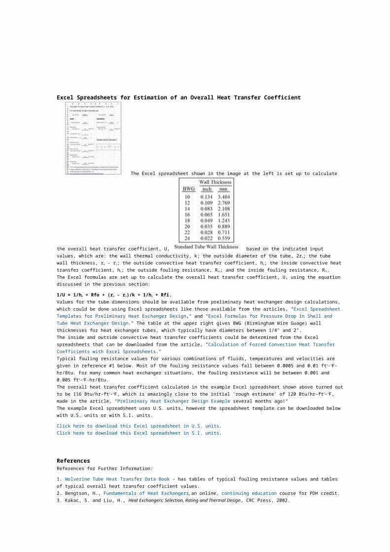
Excel Spreadsheets for Estimation of an Overall Heat Transfer Coefficient

The Excel spreadsheet shown in the image at the left is set up to calculate

the overall heat transfer coefficient, U,  based on the indicated input values, which are: the wall thermal conductivity, k; the outside diameter of the tube, 2ro; the tube wall thickness, ro - ri; the outside convective heat transfer coefficient, ho; the inside convective heattransfer coefficient, hi; the outside fouling resistance, Rfo; and the inside fouling resistance, Rfi.The Excel formulas are set up to calculate the overall heat transfer coefficient, U, using the equation discussed in the previous section:

1/U = 1/ho + Rfo + (ro - ri)/k + 1/hi + Rfi.Values for the tube dimensions should be available from preliminary heat exchanger design calculations, which could be done using Excel spreadsheets like those available from the articles, "Excel Spreadsheet Templates for Preliminary Heat Exchanger Design," and "Excel Formulas for Pressure Drop in Shell and Tube Heat Exchanger Design." The table at the upper right gives BWG (Birmingham Wire Guage) wall thicknesses for heat exchanger tubes, which typically have diameters between 1/4" and 2".The inside and outside convective heat transfer coefficients could be determined from the Excel spreadsheets that can be downloaded from the article, "Calculation of Forced Convection Heat Transfer Coefficients with Excel Spreadsheets."Typical fouling resistance values for various combinations of fluids, temperatures and velocities are given in reference #1 below. Most of the fouling resistance values fall between 0.0005 and 0.01 ft2-oF-hr/Btu. For many common heat exchanger situations, the fouling resistance will be between 0.001 and 0.005 ft2-oF-hr/Btu.The overall heat transfer coefficient calculated in the example Excel spreadsheet shown above turned outto be 116 Btu/hr-ft2-oF, which is amazingly close to the initial 'rough estimate' of 120 Btu/hr-ft2-oF, made in the article, "Preliminary Heat Exchanger Design Example several months ago!"The example Excel spreadsheet uses U.S. units, however the spreadsheet template can be downloaded below with U.S. units or with S.I. units.

Click here to download this Excel spreadsheet in U.S. units.Click here to download this Excel spreadsheet in S.I. units.

ReferencesReferences for Further Information:

1. Wolverine Tube Heat Transfer Data Book - has tables of typical fouling resistance values and tables of typical overall heat transfer coefficient values.2. Bengtson, H., Fundamentals of Heat Exchangers, an online, continuing education course for PDH credit.3. Kakac, S. and Liu, H., Heat Exchangers: Selection, Rating and Thermal Design, CRC Press, 2002.

4. Kuppan, T., Heat Exchanger Design Handbook, CRC Press, 2000.