modeling us petroleum production using standard and discounted exponential growth approaches
TRANSCRIPT
SAN FRANCISCO STATE UNIVERSITY
Modeling US Petroleum Production Using Standard and Discounted Exponential
Growth Approaches
Mark Ciotola
5/20/2010
Business 899
Supervised by Prof. Ramesh Bollapragada
SFSU BUS 899 May 2010
M. Ciotola
ii
ABSTRACT
The nature of petroleum deposits, their location and utilization is discussed. Economic factors and
general trends are also identified. Standard quantitative forecasting techniques are utilized to
forecast U.S. petroleum production. The concept of the Hewett-Hubbert curve, commonly known
as “peak oil”, is introduced. Existing methods of generating Hewett-Hubbert distributions are
demonstrated. Then, a discounted exponential growth method motivated by a proposed e th Law
of Thermodynamics is shown to generate Hewett-Hubbert distributions. The discounted
exponential growth method is then utilized to model U.S. petroleum production. Errors produced
by several standard quantitative forecasting techniques and the discounted exponential growth
method are compared.
SFSU BUS 899 May 2010
M. Ciotola
iii
Contents
EXECUTIVE SUMMARY...............................................................................................................1
SECTION 1: BACKGROUND REGARDING GLOBAL OIL GEOLOGY AND ECONOMICS.2
1.1 Why is there so much interest in oil?.......................................................................................2
1.2 What is oil and how is it formed?............................................................................................ 2
1.3 Where is oil located in the world?........................................................................................... 4
1.4 How Much Oil is There?..........................................................................................................5
1.5 How Much Oil Does the Global Economy Require? ..............................................................6
1.6 Why has Oil Become So Expensive? What Are the Current Trends on Oil............................7
1.7 Context for Production Forecasting....................................................................................... 11
SECTION 2: CONTEMPORARY PRODUCTION FORECASTING....................................... 12
2.1 Introduction............................................................................................................................11
2.2 Naive and Faith-Based Methods............................................................................................ 12
2.3 “Drill, Baby, Drill!”—Future Holes In the Ground Approach.............................................. 13
2.4 Trend Approaches, Generally................................................................................................ 13
2.5 Single Exponential Smoothing...............................................................................................14
2.6 Exponential Smoothing: Winters Method with Trend and Seasonality.................................14
2.7 Exponential Smoothing: Holt Method with Trend for Annual Data..................................... 15
2.9 Time Series Decomposition................................................................................................... 15
2.9 Regression..............................................................................................................................16
SECTION 3: DISCOUNTED EXPONENTIAL GROWTH HYPOTHESIS.................................17
Introduction..................................................................................................................................17
3.1 A Brief Introduction to Thermodynamics Fundamental Principles.......................................17
3.1.1 First Law of Thermodynamics.........................................................................................17
3.1.2 The Second Law of Thermodynamics............................................................................. 18
3.2 A Simple Thermal Conductor Bridging A Thermal Potential............................................... 20
3.3 Simple heat engine................................................................................................................. 24
3.4 Reproducing heat engines...................................................................................................... 30
3.5 Bring it all together: Generating a Hewett-Hubbert Curve Using Thermodynamics........... 32
3.6 Reproducing heat engines requiring maintenance................................................................. 33
3.7 Applying Discounted Exponential Growth to an actual example..........................................35
4 APPLICATION OF DISCOUNTED EXPONENTIAL APPROACH TO PETROLEUM
PRODUCTION............................................................................................................................38
4.1 Regional Field Hewett-Hubbert Approach............................................................................ 38
SFSU BUS 899 May 2010
M. Ciotola
iv
4.2 Hubbert basic Formula...........................................................................................................39
4.3 Discounted Exponential Growth Approach .......................................................................... 40
4.4 Discounted Exponential Growth Modeled With Iterative Program...................................... 40
4.5 Implementing Discounted Exponential Growth Modeled Analytically................................ 42
4.5.1 Efficiency Term Modeled As Simple Linear Function................................................... 43
4.5.2 Efficiency Term Modeled In Terms of Heat Flow.......................................................... 44
4.5.3 Efficiency Term Modeled In Terms of Entropy Increase................................................45
4.5.4 Comparison With Logistic Function............................................................................... 46
5 CONCLUSIONS ......................................................................................................................... 46
REFERENCES................................................................................................................................53
APPENDICES.................................................................................................................................56
Minitab Logs
Single Exponential Smoothing 1980-99
US Petroleum Production 1970-99 Decomposition
US Petroleum Production 1980-99 Decomposition
US Petroleum Production 1970-99 Regression/Trend—Linear w/Annual Data
US Petroleum Production 1970-99 Regression/Trend—Quadratic w/Annual Data
US Petroleum Production 1979-99 Regression/Trend—Linear w/Monthly Data w/ Forecast of
40 periods
US Petroleum Production 1979-99 Regression/Trend—Linear w/Monthly Data w/ Forecast of
122 periods
Minitab Charts
Single Exponential Smoothing 1980-99; Without Forecast to 2008
Single Exponential Smoothing 1980-99; With Forecast to 2008
US Petroleum Production 1980-99 Time Series Decomposition; Components
US Petroleum Production 1980-99 Time Series Decomposition; With Forecast to 2008
US Petroleum Production 1980-99 Time Series Decomposition; Seasonality
US Petroleum Production 1970-99 Regression/Trend—Linear w/Annual Data
US Petroleum Production 1970-99 Regression/Trend—Quadratic w/Annual Data
Excel Spreadsheets (may be in separate file)
US Petroleum Production 1920-2008 Naive w/Monthly
US Petroleum Production 2000-2008 Winters w/Monthly
US Petroleum Production 1970-2008 Decomposition w/Monthly
EXECUTIVE SUMMARY
The nature of petroleum deposits, their location and utilization is discussed. Economic factors and
general trends are also identified. Standard quantitative forecasting techniques are utilized to
forecast U.S. petroleum production. The concept of the Hewett-Hubbert curve, commonly known
as “peak oil”, is introduced. Such curves have been used since 1929 to model the production of
limited mineral resources such as metals or oil.1 Existing methods of generating Hewett-Hubbert
distributions are demonstrated. Then, a discounted exponential growth method motivated by a
proposed e th Law of Thermodynamics is shown to generate Hewett-Hubbert distributions. Then
it is shown how Hewett-Hubbert curves can be generated from fundamental thermodynamic
principles, using reproducing heat engines that require maintenance. The discounted exponential
growth method is then utilized to model U.S. petroleum production. Errors produced by several
standard quantitative forecasting techniques versus the discounted exponential growth method are
compared. The Winter’s Method applied to monthly data demonstrates seasonality in petroleum
production. Regression utilizing a quadratic trend is shown to reduce error when applied to
annual data. The discounted exponential growth method produces reasonable agreement over
upside modeling, but less so for downside modeling, although this may be due to error induced by
the manual choice of parameters and potential profile.
1 The author also uses Hubbert curves to model a wide range of social phenomena such as historical dynasties and economic bubbles.
SFSU BUS 899 May 2010
M. Ciotola
2
SECTION 1: BACKGROUND REGARDING GLOBAL OIL GEOLOGY AND ECONOMICS
1.1 Why is there so much interest in oil?
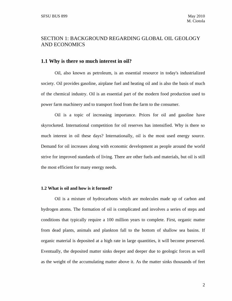
Oil, also known as petroleum, is an essential resource in today's industrialized
society. Oil provides gasoline, airplane fuel and heating oil and is also the basis of much
of the chemical industry. Oil is an essential part of the modern food production used to
power farm machinery and to transport food from the farm to the consumer.
Oil is a topic of increasing importance. Prices for oil and gasoline have
skyrocketed. International competition for oil reserves has intensified. Why is there so
much interest in oil these days? Internationally, oil is the most used energy source.
Demand for oil increases along with economic development as people around the world
strive for improved standards of living. There are other fuels and materials, but oil is still
the most efficient for many energy needs.
1.2 What is oil and how is it formed?
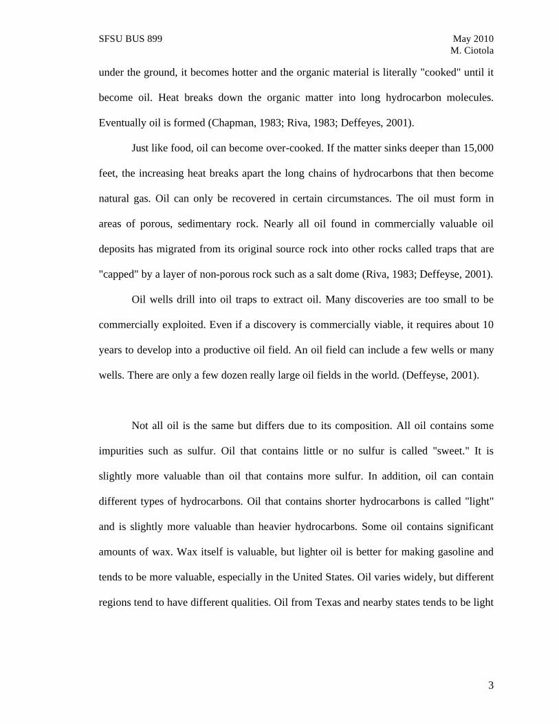
Oil is a mixture of hydrocarbons which are molecules made up of carbon and
hydrogen atoms. The formation of oil is complicated and involves a series of steps and
conditions that typically require a 100 million years to complete. First, organic matter
from dead plants, animals and plankton fall to the bottom of shallow sea basins. If
organic material is deposited at a high rate in large quantities, it will become preserved.
Eventually, the deposited matter sinks deeper and deeper due to geologic forces as well
as the weight of the accumulating matter above it. As the matter sinks thousands of feet
SFSU BUS 899 May 2010
M. Ciotola
3
under the ground, it becomes hotter and the organic material is literally "cooked" until it
become oil. Heat breaks down the organic matter into long hydrocarbon molecules.
Eventually oil is formed (Chapman, 1983; Riva, 1983; Deffeyes, 2001).
Just like food, oil can become over-cooked. If the matter sinks deeper than 15,000
feet, the increasing heat breaks apart the long chains of hydrocarbons that then become
natural gas. Oil can only be recovered in certain circumstances. The oil must form in
areas of porous, sedimentary rock. Nearly all oil found in commercially valuable oil
deposits has migrated from its original source rock into other rocks called traps that are
"capped" by a layer of non-porous rock such as a salt dome (Riva, 1983; Deffeyse, 2001).
Oil wells drill into oil traps to extract oil. Many discoveries are too small to be
commercially exploited. Even if a discovery is commercially viable, it requires about 10
years to develop into a productive oil field. An oil field can include a few wells or many
wells. There are only a few dozen really large oil fields in the world. (Deffeyse, 2001).
Not all oil is the same but differs due to its composition. All oil contains some
impurities such as sulfur. Oil that contains little or no sulfur is called "sweet." It is
slightly more valuable than oil that contains more sulfur. In addition, oil can contain
different types of hydrocarbons. Oil that contains shorter hydrocarbons is called "light"
and is slightly more valuable than heavier hydrocarbons. Some oil contains significant
amounts of wax. Wax itself is valuable, but lighter oil is better for making gasoline and
tends to be more valuable, especially in the United States. Oil varies widely, but different
regions tend to have different qualities. Oil from Texas and nearby states tends to be light
SFSU BUS 899 May 2010
M. Ciotola
4
and sweet. Fortunately, this is the best kind to refine into gasoline, given the huge
demand for gasoline in the United States (Chapman, 1983; Deffeyse, 2001).
1.3 Where is oil located in the world?
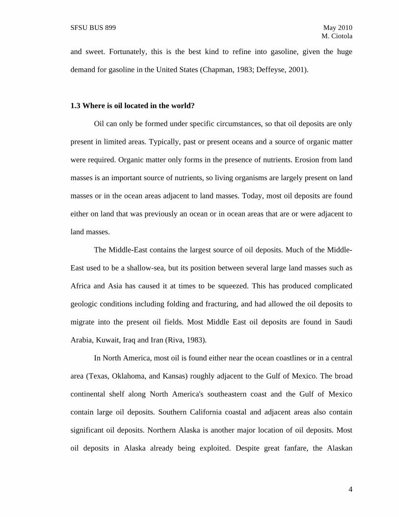
Oil can only be formed under specific circumstances, so that oil deposits are only
present in limited areas. Typically, past or present oceans and a source of organic matter
were required. Organic matter only forms in the presence of nutrients. Erosion from land
masses is an important source of nutrients, so living organisms are largely present on land
masses or in the ocean areas adjacent to land masses. Today, most oil deposits are found
either on land that was previously an ocean or in ocean areas that are or were adjacent to
land masses.
The Middle-East contains the largest source of oil deposits. Much of the Middle-
East used to be a shallow-sea, but its position between several large land masses such as
Africa and Asia has caused it at times to be squeezed. This has produced complicated
geologic conditions including folding and fracturing, and had allowed the oil deposits to
migrate into the present oil fields. Most Middle East oil deposits are found in Saudi
Arabia, Kuwait, Iraq and Iran (Riva, 1983).
In North America, most oil is found either near the ocean coastlines or in a central
area (Texas, Oklahoma, and Kansas) roughly adjacent to the Gulf of Mexico. The broad
continental shelf along North America's southeastern coast and the Gulf of Mexico
contain large oil deposits. Southern California coastal and adjacent areas also contain
significant oil deposits. Northern Alaska is another major location of oil deposits. Most
oil deposits in Alaska already being exploited. Despite great fanfare, the Alaskan
SFSU BUS 899 May 2010
M. Ciotola
5
National Wildlife Refuge contains relatively little additional oil (Chapman, 1983;
Deffeyse, 2001).
The European North Sea is also a prodigious source of oil deposits, primarily
portions that lie between the United Kingdom and Norway. Former Soviet Union states
and Indonesia are other important sources. An emerging source is the East Asian coastal
areas, which have not yet been significantly exploited due to political issues. Although
new Asian sources will be important, it is unlikely that there will be any new, extremely
large oil fields found there comparable with existing large sources such as the Middle
East oil fields (Chapman, 1983; Riva, 1983; Deffeyse, 2001).
1.4 How Much Oil is There?
Every few months, newspaper headlines make dramatic claims, such as "the U.S.
will run out of oil in 10 years" or "New Oil Field Discovered Will Supply Oil Needs for
100 years." These headlines are often misleading. One has to look at the facts behind
those figures to make sense of the global oil supply.
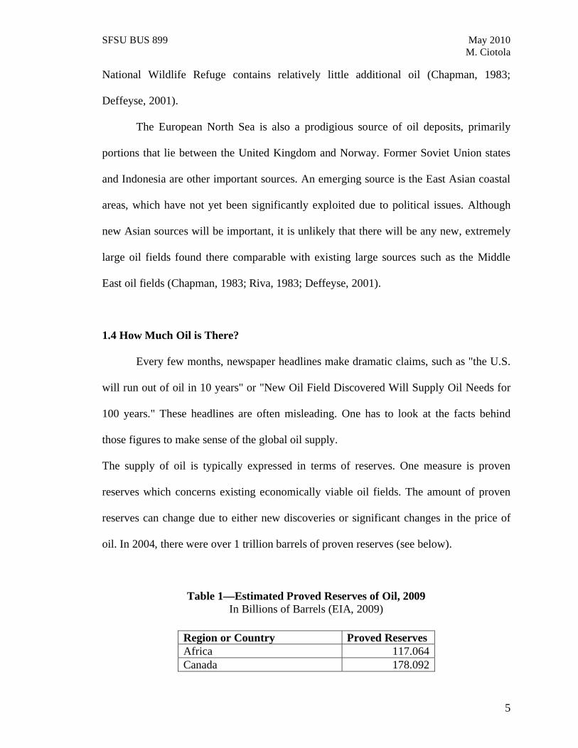
The supply of oil is typically expressed in terms of reserves. One measure is proven
reserves which concerns existing economically viable oil fields. The amount of proven
reserves can change due to either new discoveries or significant changes in the price of
oil. In 2004, there were over 1 trillion barrels of proven reserves (see below).
Table 1—Estimated Proved Reserves of Oil, 2009
In Billions of Barrels (EIA, 2009)
Region or Country Proved Reserves
Africa 117.064
Canada 178.092
SFSU BUS 899 May 2010
M. Ciotola
6
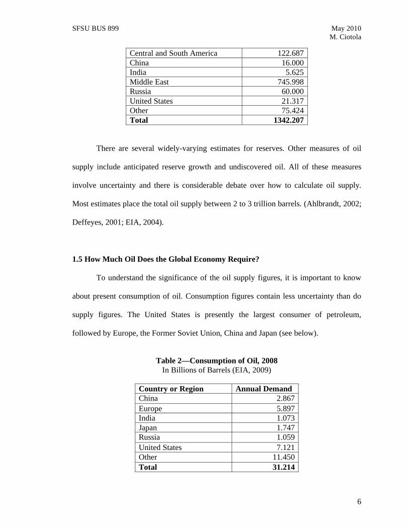
Central and South America 122.687
China 16.000
India 5.625
Middle East 745.998
Russia 60.000
United States 21.317
Other 75.424
Total 1342.207
There are several widely-varying estimates for reserves. Other measures of oil
supply include anticipated reserve growth and undiscovered oil. All of these measures
involve uncertainty and there is considerable debate over how to calculate oil supply.
Most estimates place the total oil supply between 2 to 3 trillion barrels. (Ahlbrandt, 2002;
Deffeyes, 2001; EIA, 2004).
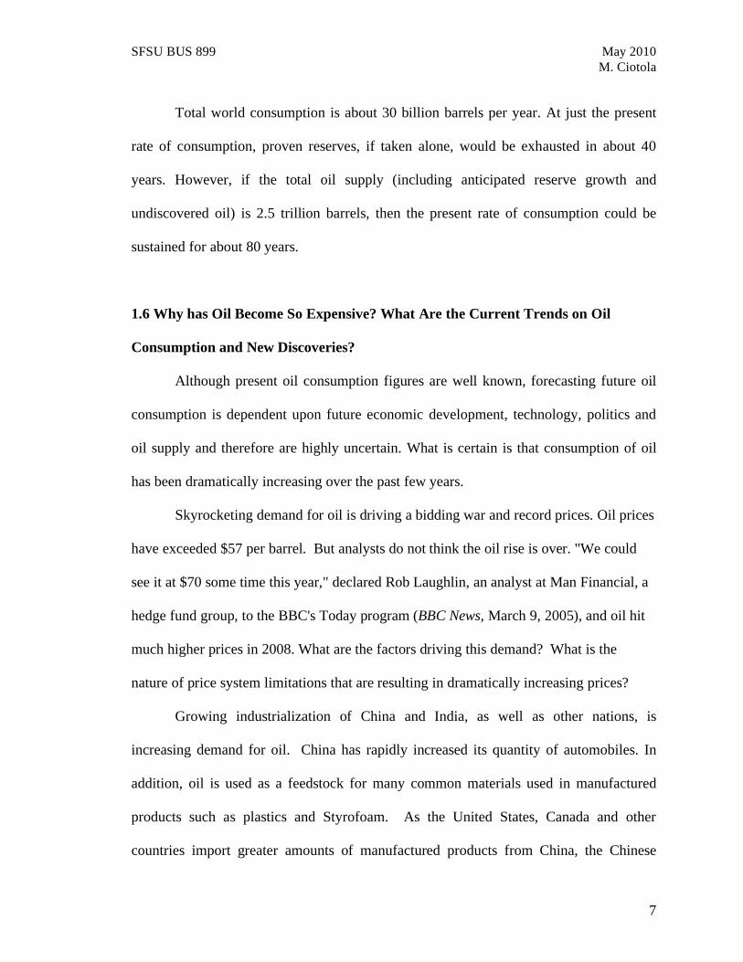
1.5 How Much Oil Does the Global Economy Require?
To understand the significance of the oil supply figures, it is important to know
about present consumption of oil. Consumption figures contain less uncertainty than do
supply figures. The United States is presently the largest consumer of petroleum,
followed by Europe, the Former Soviet Union, China and Japan (see below).
Table 2—Consumption of Oil, 2008
In Billions of Barrels (EIA, 2009)
Country or Region Annual Demand
China 2.867
Europe 5.897
India 1.073
Japan 1.747
Russia 1.059
United States 7.121
Other 11.450
Total 31.214
SFSU BUS 899 May 2010
M. Ciotola
7
Total world consumption is about 30 billion barrels per year. At just the present
rate of consumption, proven reserves, if taken alone, would be exhausted in about 40
years. However, if the total oil supply (including anticipated reserve growth and
undiscovered oil) is 2.5 trillion barrels, then the present rate of consumption could be
sustained for about 80 years.
1.6 Why has Oil Become So Expensive? What Are the Current Trends on Oil
Consumption and New Discoveries?
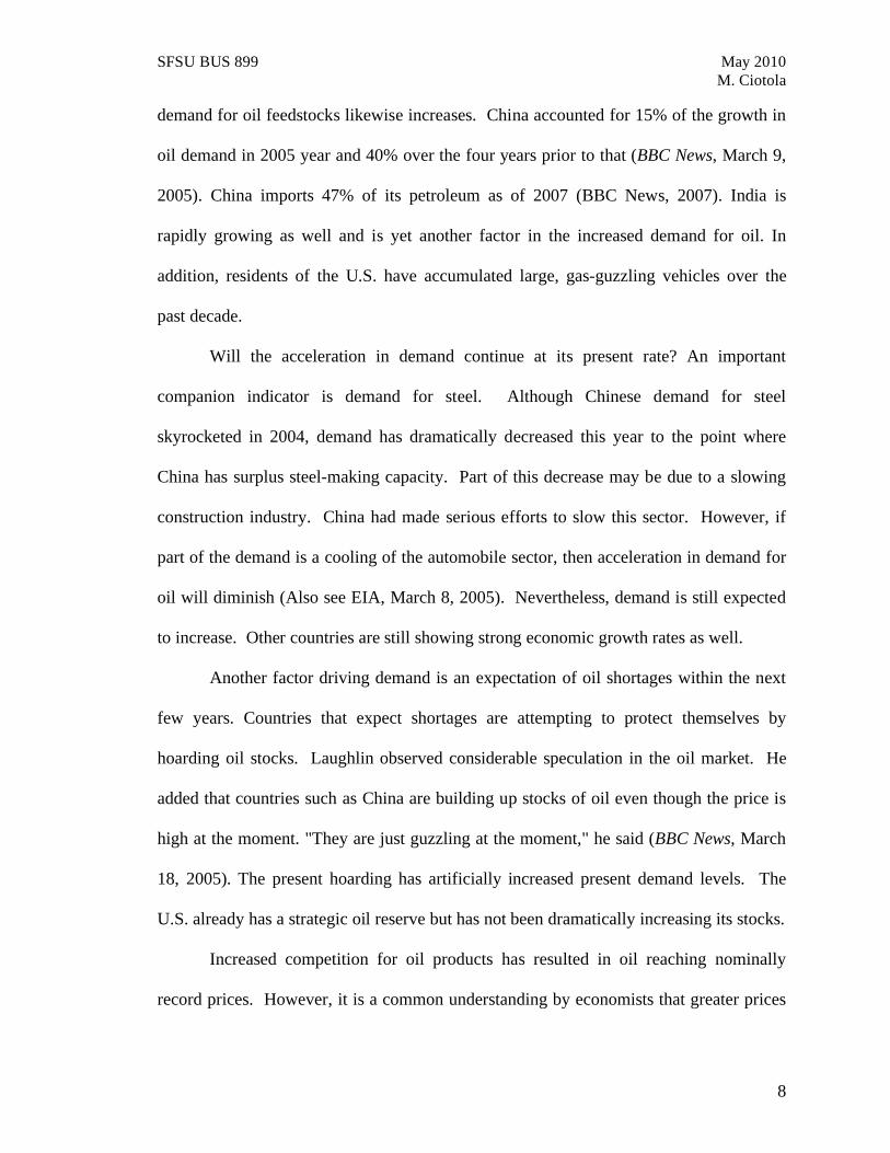
Although present oil consumption figures are well known, forecasting future oil
consumption is dependent upon future economic development, technology, politics and
oil supply and therefore are highly uncertain. What is certain is that consumption of oil
has been dramatically increasing over the past few years.
Skyrocketing demand for oil is driving a bidding war and record prices. Oil prices
have exceeded $57 per barrel. But analysts do not think the oil rise is over. "We could
see it at $70 some time this year," declared Rob Laughlin, an analyst at Man Financial, a
hedge fund group, to the BBC's Today program (BBC News, March 9, 2005), and oil hit
much higher prices in 2008. What are the factors driving this demand? What is the
nature of price system limitations that are resulting in dramatically increasing prices?
Growing industrialization of China and India, as well as other nations, is
increasing demand for oil. China has rapidly increased its quantity of automobiles. In
addition, oil is used as a feedstock for many common materials used in manufactured
products such as plastics and Styrofoam. As the United States, Canada and other
countries import greater amounts of manufactured products from China, the Chinese
SFSU BUS 899 May 2010
M. Ciotola
8
demand for oil feedstocks likewise increases. China accounted for 15% of the growth in
oil demand in 2005 year and 40% over the four years prior to that (BBC News, March 9,
2005). China imports 47% of its petroleum as of 2007 (BBC News, 2007). India is
rapidly growing as well and is yet another factor in the increased demand for oil. In
addition, residents of the U.S. have accumulated large, gas-guzzling vehicles over the
past decade.
Will the acceleration in demand continue at its present rate? An important
companion indicator is demand for steel. Although Chinese demand for steel
skyrocketed in 2004, demand has dramatically decreased this year to the point where
China has surplus steel-making capacity. Part of this decrease may be due to a slowing
construction industry. China had made serious efforts to slow this sector. However, if
part of the demand is a cooling of the automobile sector, then acceleration in demand for
oil will diminish (Also see EIA, March 8, 2005). Nevertheless, demand is still expected
to increase. Other countries are still showing strong economic growth rates as well.
Another factor driving demand is an expectation of oil shortages within the next
few years. Countries that expect shortages are attempting to protect themselves by
hoarding oil stocks. Laughlin observed considerable speculation in the oil market. He
added that countries such as China are building up stocks of oil even though the price is
high at the moment. "They are just guzzling at the moment," he said (BBC News, March
18, 2005). The present hoarding has artificially increased present demand levels. The
U.S. already has a strategic oil reserve but has not been dramatically increasing its stocks.
Increased competition for oil products has resulted in oil reaching nominally
record prices. However, it is a common understanding by economists that greater prices
SFSU BUS 899 May 2010
M. Ciotola
9
will drive the development of additional supplies that will mitigate prices. The problem
with this understanding is that supply of a natural resource cannot be arbitrarily
increased. As early as 1798, economist T. R. Malthus pointed out this principle in his
studies population and agriculture. In contemporary terms, Exxon chairman and chief
executive Lee Raymond told analysts: "We are in the mode where the fundamentals of
supply and demand really don't drive the price. High oil prices fail to lift oil stock (BBC
News, 18 March, 2005)." For example, China's output only rose 2% last year.
Improved technology such as Global Positioning Systems (GPS) and advanced seismic
techniques have been utilized to discover additional reserves. To give economists some
credit, the amount of recoverable oil in the ground is partially a factor of price. Despite
record use of oil, reserved have actually slightly increased over the past year. Higher
prices justify higher recovery costs.
Unfortunately newly-discovered reserves tend to be located in environmentally or
politically sensitive areas. "Much of the new production in the 1990s has come from the
developing countries of Latin America, West Africa, the non-OPEC Middle East, and
China." In fact, production from such sources is expected to increase "from 46.7 million
barrels per day in 2001 to 64.6 million barrels per day in 2025" (EIA, 2004). To put that
in perspective, "U.S. oil demand averaged 20.5 million barrels per day in 2004 (EIA,
2005)."
Also, new technologies are better at discovering offshore oil deposits. The
potential for environmentally disastrous leaks is significant. The Artic is another
controversial source of oil. "Arctic basins with about 25% of undiscovered oil resources"
(Ahlbrandt, 2002). Despite the political fanfare over drilling the Artic Wildlife Reserve in
SFSU BUS 899 May 2010
M. Ciotola
10
Alaska, that region contained relatively little oil. The bulk of Alaska's oil resources are
already being exploited (Deffeyes, 2001).
In addition, such reserves are more expensive to exploit since they are offshore or
in remote areas (EIA, 2004). Deposits in Africa and South America are often in remote
jungles. Offshore deposits require expensive drilling rigs and deep drilling. Artic areas
typically involve drilling through hundreds of meters of permafrost.
Yet despite increased reserves, oil prices have still dramatically increased. Causes
of these increases can be traced to increased competition for oil products, the expectation
in future increases in demand as well as the inability of the oil production infrastructure
to keep pace with growing demand.
There is still plenty of oil in the ground for at least the next few decades, so why
have prices increased so dramatically? The reason is only partly related to supply. Oil in
the ground is a much different matter than immediate supply. Immediately prior to the
U.S. 2004 Presidential election, Saudi Arabia was producing every barrel it could
squeeze out of its wells, yet prices remained high. The problem is two-fold. For the
immediate timeframe, the oil production, transportation and refining infrastructure is
relatively fixed. When demand increases quickly, the infrastructure operates at full
capacity, and so excessive demand creates a bidding war.
Infrastructure can be expanded over a period of several years. However, in a
business environment that focuses on quarterly profits, infrastructure expansion is
undesirable. Recall that 10 years is typically required to develop an oil discovery into a
productive oil field. Pipelines and refineries are expensive to build. So infrastructure
expansion creates short-term losses rather than short-term profits. CEO compensation
SFSU BUS 899 May 2010
M. Ciotola
11
rarely emphasizes the company's performance 10 years in the future. So relatively little
business incentive exists to expand infrastructure to meet increased demand. However,
governments can help to develop infrastructure through political pressure and incentives.
As infrastructure grows to meet demand, prices increases will stabilize. Nevertheless, the
long-term price of oil can be expected to increase as demand increases but supply
remains limited.
1.7 Context for Production Forecasting
Oil requires about 100 million years to form, about 10 years to develop and
exploit, and less than ten seconds to burn. Most oil is found in past or present ocean
environments such as the Middle East, the Gulf of Mexico, the North Sea or adjacent
areas such as Texas. There is an estimated 2 to 3 trillion barrels of commercially
exploitable oil already discovered or anticipated to be discovered. Present oil
consumption is 30 billion barrels per year, but has been dramatically increasing over the
past few years. Presently high oil prices are due to increased demand exceeding
production and delivery infrastructure as well as investor speculation that demand for oil
will continue to skyrocket. As infrastructure catches up with increased demand, price
increases should slow, but not disappear. There are sufficient oil reserves to meet demand
for at least the next few decades, although present levels of consumption cannot be
maintained indefinitely.
SECTION 2: CONTEMPORARY PRODUCTION FORECASTING
2.1 Introduction
SFSU BUS 899 May 2010
M. Ciotola
12
Several contemporary methods exist for oil production forecasting, ranging from
sophisticated to simple, from scientific to faith-based. There may be a commonly-
believed analogy regarding oil forecasting to the Heisenberg Uncertainty Principle in
Physics: the act of forecasting oil production will affect the actual level of oil production
(author observation). Therefore, forecasting petroleum production is fraught with
political and even religious implications. Putting politics largely aside, this section will
attempt to catalog major forecasting techniques, and discuss the strengths and weaknesses
of each from physical and quantitative viewpoints.
Actual petroleum production data is obtained by the Energy Information
Administration (EIA), a division of the United States Department of Energy. EIA data is
a widely-recognized benchmark for U.S. production data (the author found no significant
controversies regarding EIA data when concerning U.S. production).
2.2 Naive and Faith-Based Methods
The Naive Method results in a forecast that is identical to data from the most
recent observed period. Specifically, “naive forecasts assume that recent periods are the
best predictors of the future” (Hanke and Wichern, 2005). So the Naive Method would
forecast that oil production will continue at the same level as in the most recent period,
such as the last year. Some faith-based methods propose a physical mechanism to support
the naive method, that supernatural forces replace oil that is removed from the ground,
thereby ensuring a perpetual supply (e.g., see Akers, 2007). Naive and faith-based
methods are not unreasonable approaches for rough forecasts within a period of a few
SFSU BUS 899 May 2010
M. Ciotola
13
years, since new oil production infrastructure can take several years to build, and new oil
fields can easily take a decade or more to develop (see Section 1).
[See Appendices for Excel printout]
2.3 “Drill, Baby, Drill!”—Future Holes In the Ground Approach
The “Future Holes in the Ground” approach states that future oil production is a
function of the quantity of oil fields developed and wells placed in the ground. Since it
typically takes a decade to develop a new oil field, this approach is no better than the
naive method for shorter periods. For periods ranging from a decade to a few decades,
this approach may be effective (author opinion), since there still exist large, relatively
unexploited oil fields, such as in Iran (Deffayse, 2001), but since there are only a limited
quantity of such fields, this approach will likely not provide accurate forecasts be
effective beyond a few decades. This approach assumes that demand will rise to meet
production; the popularity of the Hummer and SUVs as a response to the relatively cheap
petroleum bubble of the 1990s supports this assumption (author observation). It also
assumes that the oil industry can drill as many holes as it desires, as long as the U.S.
public supports military intervention (available in unlimited quantities) in other countries
where needed, such as Iraq and Iran. This assumption is in part valid (the U.S. did invade
Iraq), but not entirely valid (any such plans that have existed to invade Iran have so far
not occurred). This approach can be summed up by a popular U.S. political mantra:
“Drill, Baby, Drill!”
2.4 Trend Approaches, Generally
SFSU BUS 899 May 2010
M. Ciotola
14
Trend approaches identify trends in historic data and then extrapolates those
trends into forecasts (text). Such trends, when using averaging and accounting for cycles,
are often effective for forecasting where linear, quadratic and even exponential trends
exist (Hanke and Wichern, 2005). However, they may fall short when there are more
complex mechanisms affecting the data over time. Complex, multi-component
exponential curves can change quickly (e.g., see Meadows et al, 1972).
2.5 Simple Exponential Smoothing
Simple exponential smoothing method attempts to forecast data by averaging data
for several past periods, so that single period variations do not skew forecasts. However,
smoothing is in a manner that is biased towards most recent data (Hanke and Wichern,
2005). For example, simple exponential smoothing might help minimize the impact of a
one-time hurricane event.
[See Appendices for Excel and Minitab printouts]
2.6 Exponential Smoothing: Winters Method with Trend and Seasonality
The Winters method involves exponential smoothing, but it also captures trend
and seasonality components (Hanke and Wichern, 2005). The Winters method improves
forecast when seasonal data is involved. Since seasonality is involved in U.S. petroleum
production, the Winters method is utilized here for analyzing monthly petroleum
production data.
SFSU BUS 899 May 2010
M. Ciotola
15
[See Appendices for Excel and Minitab printouts]
2.7 Exponential Smoothing: Holt Method with Trend for Annual Data
The Holt method is similar to the Winters method, but does not take seasonality
into account. The Holt method involves exponential smoothing, but it also captures a
trend component. The Holt method can account for linear trends or even simple
exponential or quadratic trends. The Holt method is most appropriate to analyze to annual
data where any seasonality have been averaged out when used to analyze petroleum
production.
[See Excel and Minitab printouts]
2.8 Time Series Decomposition
Decomposition involves separating the components of time series data by trend
and seasonality. Minitab was utilized to perform decomposition on U.S. petroleum
production data from January 1970 to December 1999. (See Minitab printout and graphs
and Excel data table in Appendices).
Seasonality was indicated, but it was not a smooth change from month to month.
Production was especially low during January; this could be due to difficulties
transporting oil from Alaska’s Prudhoe Bay during especially cold weather (author
speculation), since crude oil can solidify when cold.
SFSU BUS 899 May 2010
M. Ciotola
16
A forecast was then made from January 2000 to December 2009. (See Minitab
printout and graphs and Excel data table in Appendices).
SUMMARY OF MINITAB PRINTOUT
Multiplicative Model
Fitted Trend Equation: Yt = 282374 - 420.937*t Seasonal Indices
Month Index Month Index 1 1.02314 2 0.92934 3 1.02463 4 0.99138 5 1.01979 6 0.98262
7 1.01041 8 1.00651 9 0.98042 10 1.02164 11 0.98736 12 1.02275
Accuracy Measures
MAPE 3 MAD 7402 MSD 89458039
2.9 Regression
Decomposition involves separating the components of time series data by trend and
seasonality. Minitab was utilized to perform decomposition on U.S. petroleum production data
from January 1970 to December 1999. (See Minitab printout, graphs and Excel data table in
Appendices). Both linear and quadratic trends were modeled. The quadratic trend provided a
better fit (lower MSE, etc.).
SFSU BUS 899 May 2010
M. Ciotola
17
MINITAB PRINTOUT
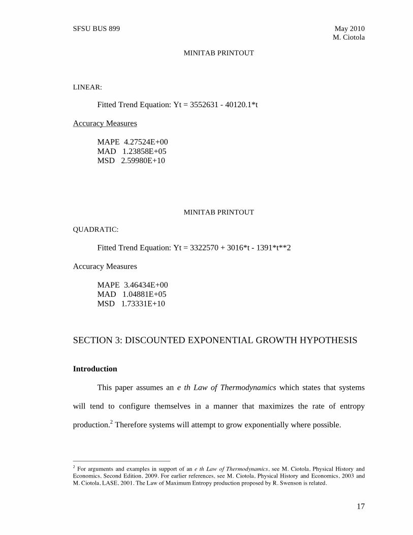
LINEAR:
Fitted Trend Equation: Yt = 3552631 - 40120.1*t Accuracy Measures
MAPE 4.27524E+00 MAD 1.23858E+05 MSD 2.59980E+10
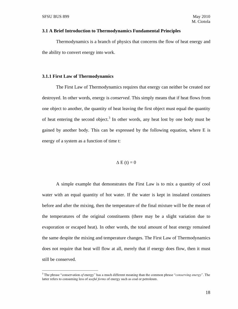
MINITAB PRINTOUT
QUADRATIC:
Fitted Trend Equation: Yt = 3322570 + 3016*t - 1391*t**2
Accuracy Measures
MAPE 3.46434E+00 MAD 1.04881E+05 MSD 1.73331E+10
SECTION 3: DISCOUNTED EXPONENTIAL GROWTH HYPOTHESIS
Introduction
This paper assumes an e th Law of Thermodynamics which states that systems
will tend to configure themselves in a manner that maximizes the rate of entropy
production.2 Therefore systems will attempt to grow exponentially where possible.
2 For arguments and examples in support of an e th Law of Thermodynamics, see M. Ciotola, Physical History and Economics, Second Edition, 2009. For earlier references, see M. Ciotola, Physical History and Economics, 2003 and M. Ciotola, LASE, 2001. The Law of Maximum Entropy production proposed by R. Swenson is related.
SFSU BUS 899 May 2010
M. Ciotola
18
3.1 A Brief Introduction to Thermodynamics Fundamental Principles
Thermodynamics is a branch of physics that concerns the flow of heat energy and
the ability to convert energy into work.
3.1.1 First Law of Thermodynamics
The First Law of Thermodynamics requires that energy can neither be created nor
destroyed. In other words, energy is conserved. This simply means that if heat flows from
one object to another, the quantity of heat leaving the first object must equal the quantity
of heat entering the second object.3 In other words, any heat lost by one body must be
gained by another body. This can be expressed by the following equation, where E is
energy of a system as a function of time t:
E (t) = 0
A simple example that demonstrates the First Law is to mix a quantity of cool
water with an equal quantity of hot water. If the water is kept in insulated containers
before and after the mixing, then the temperature of the final mixture will be the mean of
the temperatures of the original constituents (there may be a slight variation due to
evaporation or escaped heat). In other words, the total amount of heat energy remained
the same despite the mixing and temperature changes. The First Law of Thermodynamics
does not require that heat will flow at all, merely that if energy does flow, then it must
still be conserved.
3 The phrase “conservation of energy” has a much different meaning than the common phrase “conserving energy”. The latter refers to consuming less of useful forms of energy such as coal or petroleum.
SFSU BUS 899 May 2010
M. Ciotola
19
3.1.2 The Second Law of Thermodynamics
The Second Law of Thermodynamics states that if heat does flow, then overall, a
quantity called entropy will tend to increase.4
Entropy before heat flow Entropy after heat flow,
or
S(t0) S(t1),
where S is entropy and t is time.
Entropy has a precise meaning in physics that can be found in advanced textbooks
dedicated to thermodynamics. For now, we just need to recognize that when a closed
system has reached equilibrium, its entropy is at a maximum. The further away a closed
system is from equilibrium, the lower its entropy will tend to be. An example of a system
at equilibrium is in the above water-mixing example after the water has been mixed and
all becomes the same temperature.
Stated another way, the entropy of an isolated system away from equilibrium shall
tend to increase.5,6 A corollary is that a system will approach a state of maximum entropy
4 Specifically, the entropy of an isolated system shall tend to increase. A more precise definition is that “any large system in equilibrium will be found in the macrostate with the greatest multiplicity (aside from fluctuations that are normally too small to measure).” D. Schroeder, An Introduction to Thermal Physics. San Francisco: Addison-Wesley, 2002. 5 A more precise definition is that “any large system in equilibrium will be found in the macrostate with the greatest multiplicity (aside from fluctuations that are normally too small to measure).” D. Schroeder, An Introduction to Thermal Physics. San Francisco: Addison-Wesley, 2002. 6The Second Law states that the entire universe is moving towards greater entropy. The entire universe can be viewed as an isolated system.
SFSU BUS 899 May 2010
M. Ciotola
20
if given enough time.7 A system in a state of maximum entropy is in essence a system in
equilibrium. However, the Second Law does not describe the rate at which entropy shall
be produced, nor how long it would take a system to produce maximum entropy.
There are commonly several situations, in addition to heat flow, where entropy
increases. When Many chemical reactions result in increases of entropy, such as when
gasoline is combusted to propel an automobile. Entropy is increased when substances
become more mixed even where no chemical reaction occurs, such as when helium and
neon gasses become mixed together. Chemical reactions, such as burning coal and oil or
metabolizing sugars also results in entropy production.
3.2 A Simple Thermal Conductor Bridging A Thermal Potential
Most introductory physics textbooks do have an example concerning
thermodynamics that involves time.8 This example concerns a simple thermal conductor
through which energy flows from a warmer reservoir to the cooler reservoir. In most
textbooks, the term reservoir refers to a body whose temperature remains constant
regardless of how much heat energy flows in or out of it.9 However, in this paper, the
temperature of a reservoir will change depending on whether energy is added to or
removed from it.
7 Recall our simple thermal conductor example. As heat energy moves from the warmer to the cooler region, entropy is produced. 8 One can infer the passage of time by multiplying the calculated heat flow by time. However, this is example is not really time dependent. The heat flow remains constant regardless of how much time passes in this idealized example. It is nevertheless a good approximation for many real situations. 9 Heat flow is also proportional to the difference in two temperatures that the thermal conductor bridges. This difference has nothing to do with the conductors themselves. Heat flows through a thermal conductor in proportion to the area of the conductor as well as its thermal conductivity. More heat will flow through a broad conductor than a narrow one. Also, more heat will flow through a material with a high thermal conductivity such as aluminum than through a material with low thermal conductivity such as wood. Heat flow is inversely proportional to the conductor's length. More heat will flow through a shorter conductor than a long one. This is known as Fourier’s heat conduction law
SFSU BUS 899 May 2010
M. Ciotola
21
Recalling the First Law of Thermodynamics, any heat lost by one body must be
gained by another body. The quantity of heat energy lost by the warmer reservoir is
identical to the quantity of heat energy gained by the cooler reservoir:
Heat lost by warmer reservoir = Heat gained by cooler reservoir
Recalling the Second Law of Thermodynamics, if heat flows from the warmer
reservoir to the cooler reservoir, then the total entropy of this system increases. The
entropy of a cooler reservoir increases as its temperature increases. Conversely, if a
warmer reservoir’s temperature decreases as it loses heat energy, then its entropy will
decrease.
In this example, the heat lost by the warmer reservoir is gained by the cooler
reservoir. The magnitude of the entropy increase of the cooler body is greater than the
magnitude of entropy loss by the warmer body, so the total entropy of the combined
warmer reservoir - cooler reservoir system increases.
Picture a well-insulated container of hot water and another of cold water.10 The
container of hot water constitutes a warmer body, which we will call the hot reservoir.
The container of cold water represent a cooler body, which we will call the cold
reservoir. A copper bar thermally bridges the two containers so that heat can flow from
the hot container to the cold container.
Entropy = Entropy (hot reservoir) + entropy (cold reservoir)
10 If ice water is used, then energy due to the phase change of melting ice must also be accounted for.
SFSU BUS 899 May 2010
M. Ciotola
22
Potential entropy is represented by the difference between the quantity of entropy
when equilibrium is reached minus the quantity of entropy before any heat flow takes
place. This will be a positive number. An expression for potential entropy in this case is
the following equation, where m is the mass of the water in each reservoir, c is the
specific heat of water, T is temperature, and R is potential entropy, f refers to final, i
refers to initial, H refers to hot and C refers to cold:
R = mH cwater ln ( TH f / TH i ) + mC cwater ln ( TC f / TC i )
It should be noted that
TH f = TC f
which is the equivalent of stating that the a system has reached equilibrium. In
this context, the terms Hot and Cold refer to specific containers rather than the state of
those containers.
Entropy at the beginning is:
S = mH cwater TH i + mC cwater TC i
Entropy at end is:
S = mH cwater TH f + mC cwater TC f
SFSU BUS 899 May 2010
M. Ciotola
23
Or more simply,
S = ( mH + mC ) cwater T f
Heat flow through a thermal conductor is proportional to the area of the conductor
as well as its thermal conductivity. More heat will flow through a broad conductor than a
narrow one. Also, more heat will flow through a material with a high thermal
conductivity such as aluminum than through one with low thermal conductivity such as
wood. Heat flow is inversely proportional to the conductor's length. Thus, more heat will
flow through a short conductor than a long one.
Heat flow is also proportional to the difference in two temperatures that the
thermal conductor bridges. This difference in temperatures has nothing to do with the
conductors themselves. A greater temperature difference will provide a greater heat flow
across a given conductor, regardless of the characteristics of that conductor.
The equation for heat flow through a conductor is known as Fourier’s Conduction
Law11, where Q is heat flow, k is a thermal constant, A is conductor area, T is
temperature, x is conductor length and t is time:
Q / t = k A T / x
11 Electrical engineers will find this equation similar to an arrangement of Ohms Law, where electric current is proportional to voltage divided by resistance (I = V/R).
SFSU BUS 899 May 2010
M. Ciotola
24
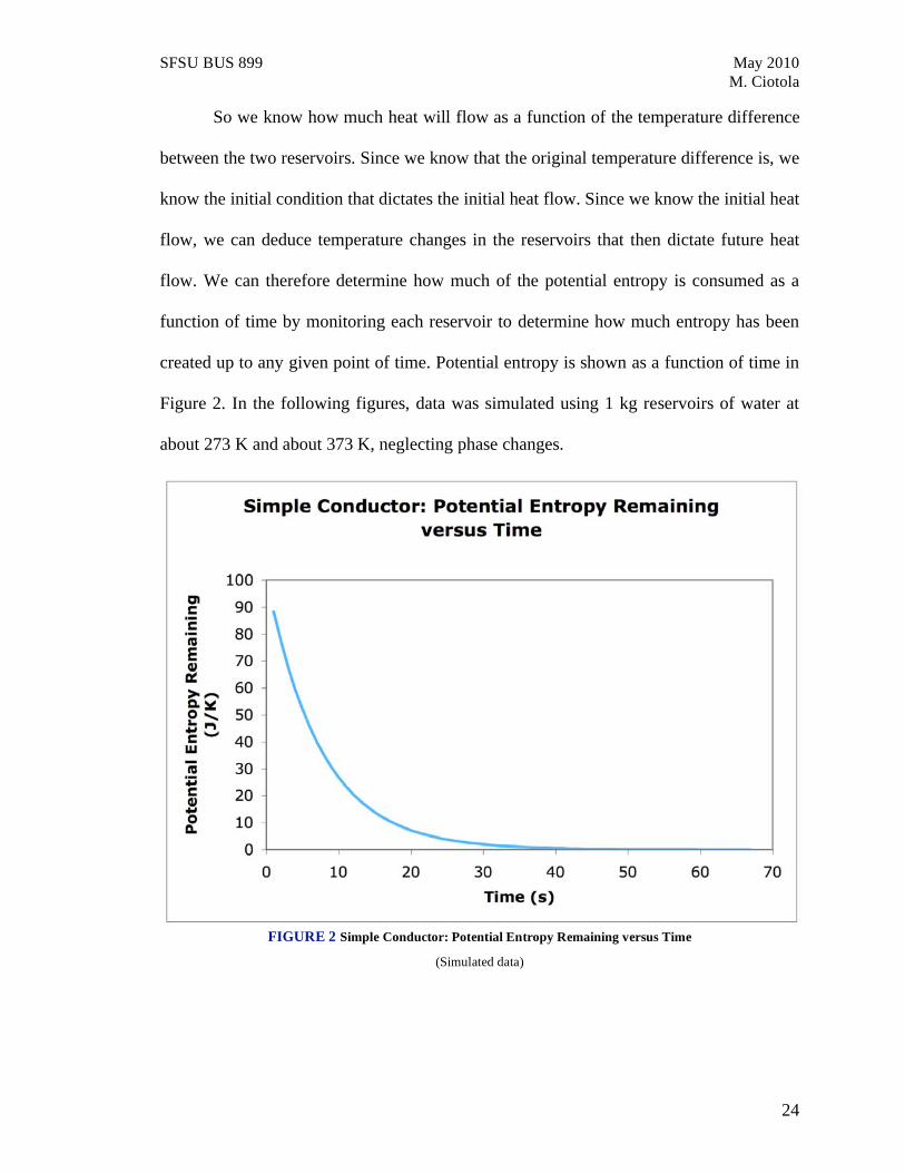
So we know how much heat will flow as a function of the temperature difference
between the two reservoirs. Since we know that the original temperature difference is, we
know the initial condition that dictates the initial heat flow. Since we know the initial heat
flow, we can deduce temperature changes in the reservoirs that then dictate future heat
flow. We can therefore determine how much of the potential entropy is consumed as a
function of time by monitoring each reservoir to determine how much entropy has been
created up to any given point of time. Potential entropy is shown as a function of time in
Figure 2. In the following figures, data was simulated using 1 kg reservoirs of water at
about 273 K and about 373 K, neglecting phase changes.
FIGURE 2 Simple Conductor: Potential Entropy Remaining versus Time
(Simulated data)
SFSU BUS 899 May 2010
M. Ciotola
25
3.3 Simple heat engine
A common example used to illustrate the Second Law is the Heat Engine. To
power a heat engine to function, heat must flow across a temperature difference,12 from a
warmer region to a cooler one. A heat engine uses temperature differences to perform
work. When heat flows to power a heat engine, part of the available energy is put into
work and the remainder results in waste heat. An example is the temperature difference
between a hot flame and a cool tank of water being used in a steam engine.
No engine turns all of the heat flow into work. That would imply 100%
efficiency, which is impossible in theory13
as well as practice, regardless of how well the
engine is constructed. The Second Law of Thermodynamics tells that even the best
engines will produce entropy along with work. The best efficiency that an ideal engine
can achieve is known as its Carnot Efficiency. The Carnot Efficiency is simply the
difference between the warmer and cooler temperature divided by the warmer
temperature. In reality, most engines are a great deal less efficient than even the Carnot
efficiency. Several modern means exist to utilize higher order energy. The equation for
Carnot Efficiency is:
Carnot Efficiency = 1 – (cooler temperature/warmer temperature)
Absolute temperatures must be used to calculate the Carnot Efficiency. Absolute
temperatures are measured from absolute zero, which is the lowest possible temperature
12 Incidentally, a heat engine is a system that has pure physical aspects as well as social aspects. 13 Unless the cold reservoir is at a temperature of absolutely zero, which is nearly impossible, statistically speaking.
SFSU BUS 899 May 2010
M. Ciotola
26
in theory, and has never been quite obtained in practice. Such temperatures are measured
in a kind of degree called Kelvin. 0° Celsius equals about 273 Kelvin.
An example is the temperature difference between a hot flame and a cool tank of
water being used in a steam engine. Then, part of the available energy is used to perform
work and the remainder is exhausted as waste heat. For instance, a steam engine could
contain a piston that converts some of the heat flow into a cyclic in-out motion that
represents work done upon a load, such as a flywheel wheel. Steam released into cooler
air represents waste heat. When waste heat is created, an intangible quantity called
entropy is produced. The more the heat engine works, the more entropy it will produce.14
If heat flows from a warmer object to a cooler object (where no engine is
involved), no work results, but entropy is still produced (or you could say that the entropy
of the system under consideration increases). For example, thermal conduction results in
lots of entropy production but little work. A thermal conductor can be thus thought of as
a lazy heat engine. If a heat engine operates at less than the Carnot ideal, entropy
increases. This is the case for all real heat engines.
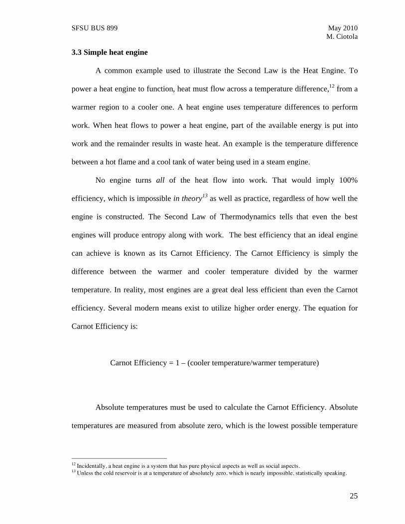
A simple heat engine "heat engine" is shown in Figure 3. Most technical details
have been omitted. Here, a tank of water that is presumably heated into high-pressure
steam by a flame or other energy source. The tank contains a piston that converts some of
that heat energy into a cyclic in-out motion that represents work done upon a load, here
represented by the wheel. The little puffs of steam represents the waste heat.
14 In theory, a heat engine is not required to produce entropy if the temperature of the cold region is absolute zero (which is about – 273° C). In practice, such a low temperature is physically impossible.
SFSU BUS 899 May 2010
M. Ciotola
27
FIGURE 3 Simple heat engine
Heat engines need to work between warmer and cooler heat reservoirs. Warmer
heat reservoirs can be flames, hot air or steam, for example. Cooler heat reservoirs can be
ice, cold air or cool water, for example. Air at room temperature can serve as either kind
of reservoir depending on how hot or cold the other reservoir is.
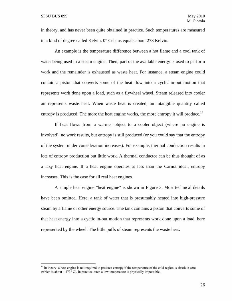
Here we see a heat engine working between a warmer reservoir and a cooler
reservoir, left and right, respectively (Fig. 4). Warmth is represented by greater height
and redder shading (if your version is in color). The higher and redder the left heat
reservoir, the hotter is it. Conversely, coolness is represented by lower height and bluer
shading. The lower and bluer the cooler heat reservoir, the colder it is. Our heat engine
begins operating between a quite hot and a quite cold reservoir as shown here (Figure 4).
FIGURE 4 Heat engine operating between thermal reservoirs
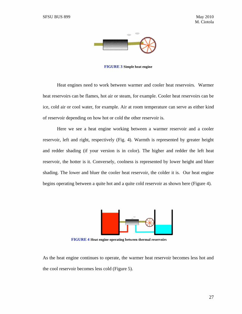
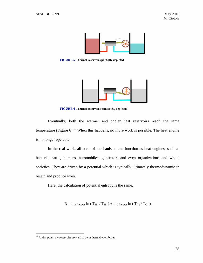
As the heat engine continues to operate, the warmer heat reservoir becomes less hot and
the cool reservoir becomes less cold (Figure 5).
SFSU BUS 899 May 2010
M. Ciotola
28
FIGURE 5 Thermal reservoirs partially depleted
FIGURE 6 Thermal reservoirs completely depleted
Eventually, both the warmer and cooler heat reservoirs reach the same
temperature (Figure 6).15 When this happens, no more work is possible. The heat engine
is no longer operable.
In the real work, all sorts of mechanisms can function as heat engines, such as
bacteria, cattle, humans, automobiles, generators and even organizations and whole
societies. They are driven by a potential which is typically ultimately thermodynamic in
origin and produce work.
Here, the calculation of potential entropy is the same.
R = mH cwater ln ( TH f / TH i ) + mC cwater ln ( TC f / TC i )
15 At this point, the reservoirs are said to be in thermal equilibrium.
SFSU BUS 899 May 2010
M. Ciotola
29
Potential is represented by the amount of entropy when equilibrium is reached minus
entropy at beginning of time.
Entropy at beginning is:
S = mH cwater TH i + mC cwater TC i
Entropy at end is:
S = mH cwater TH f + mC cwater TC f
However, here is where the examples diverge. Instead of a simple thermal
conductor bridging the thermal difference following Fourier’s Conduction Law, we are
now considering a heat engine. The amount of heat transferred by the heat engine is a
fixed about that we set arbitrarily. Once set, it does not change. For example, we could
set the heat engine to transfer 10 MJ per day.
Although the heat engine produces work, that work cannot exceed the amount of
energy transferred. In fact, it will be less.
Q = heat removed from hot reservoir – heat put into work
The percentage of energy removed that is turned into work is the engine’s
efficiency. The efficiency for the engine is a function of potential. The higher the
potential, the higher the efficiency.
SFSU BUS 899 May 2010
M. Ciotola
30
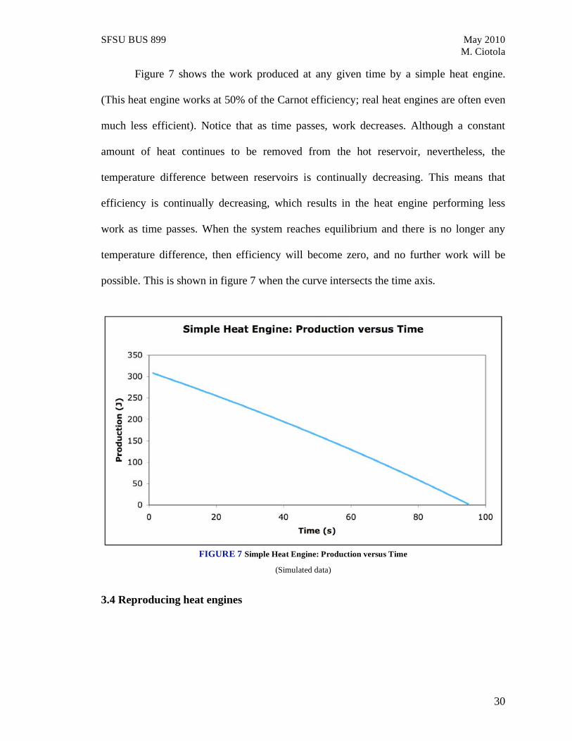
Figure 7 shows the work produced at any given time by a simple heat engine.
(This heat engine works at 50% of the Carnot efficiency; real heat engines are often even
much less efficient). Notice that as time passes, work decreases. Although a constant
amount of heat continues to be removed from the hot reservoir, nevertheless, the
temperature difference between reservoirs is continually decreasing. This means that
efficiency is continually decreasing, which results in the heat engine performing less
work as time passes. When the system reaches equilibrium and there is no longer any
temperature difference, then efficiency will become zero, and no further work will be
possible. This is shown in figure 7 when the curve intersects the time axis.
FIGURE 7 Simple Heat Engine: Production versus Time
(Simulated data)
3.4 Reproducing heat engines
SFSU BUS 899 May 2010
M. Ciotola
31
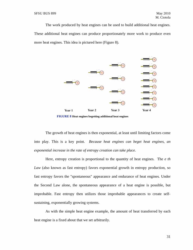
The work produced by heat engines can be used to build additional heat engines.
These additional heat engines can produce proportionately more work to produce even
more heat engines. This idea is pictured here (Figure 8).
FIGURE 8 Heat engines begetting additional heat engines
The growth of heat engines is then exponential, at least until limiting factors come
into play. This is a key point. Because heat engines can beget heat engines, an
exponential increase in the rate of entropy creation can take place.
Here, entropy creation is proportional to the quantity of heat engines. The e th
Law (also known as fast entropy) favors exponential growth in entropy production, so
fast entropy favors the "spontaneous" appearance and endurance of heat engines. Under
the Second Law alone, the spontaneous appearance of a heat engine is possible, but
improbable. Fast entropy then utilizes those improbable appearances to create self-
sustaining, exponentially growing systems.
As with the simple heat engine example, the amount of heat transferred by each
heat engine is a fixed about that we set arbitrarily.
SFSU BUS 899 May 2010
M. Ciotola
32
Let’s assume 300 J of the work is required to build new heat engines. Let’s further
assume new engines are produced instantaneously at the end of each day and put into
commission at the beginning of each next day. Then heat transferred for the second day
will be due to two heat engines. On the third day due to even more heat engines. So as
long as the potential remains high, the quantity of heat engines, this the quantity of heat
transfer grows exponentially. (Note that the data was simulated in seconds rather than
days; in a real mining region Hubbert curve, building new “engines” may require days or
even years. However, the underlying concepts still apply).
3.5 Bring it all together: Generating a Hewett-Hubbert Curve Using
Thermodynamics
Despite the growing population of heat engines, since the amount of potential is
limited, then the efficiency will begin to drop. Consequently, the amount of work each
heat engine produces drop, even though it still transfers the same amount of energy. So
for a while, the amount of heat engines and total heat transferred may continue to
increase, but the rate of increase will slow down. Eventually efficiency drops to a point
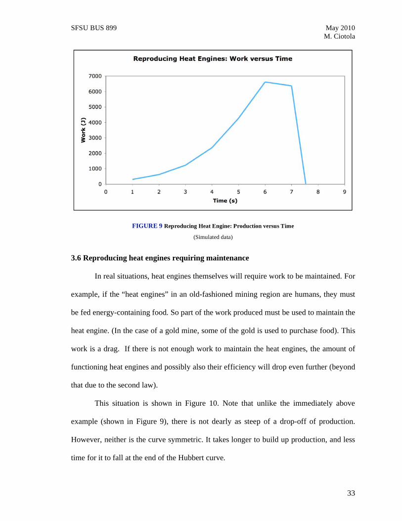
where production drops to zero. In this case, the drop-off is quite sudden and may happen
instantaneously. This results of the situation are shown in Figure 9. Partial heat engines
were allowed to be built in this simulation.
SFSU BUS 899 May 2010
M. Ciotola
33
FIGURE 9 Reproducing Heat Engine: Production versus Time
(Simulated data)
3.6 Reproducing heat engines requiring maintenance
In real situations, heat engines themselves will require work to be maintained. For
example, if the “heat engines” in an old-fashioned mining region are humans, they must
be fed energy-containing food. So part of the work produced must be used to maintain the
heat engine. (In the case of a gold mine, some of the gold is used to purchase food). This
work is a drag. If there is not enough work to maintain the heat engines, the amount of
functioning heat engines and possibly also their efficiency will drop even further (beyond
that due to the second law).
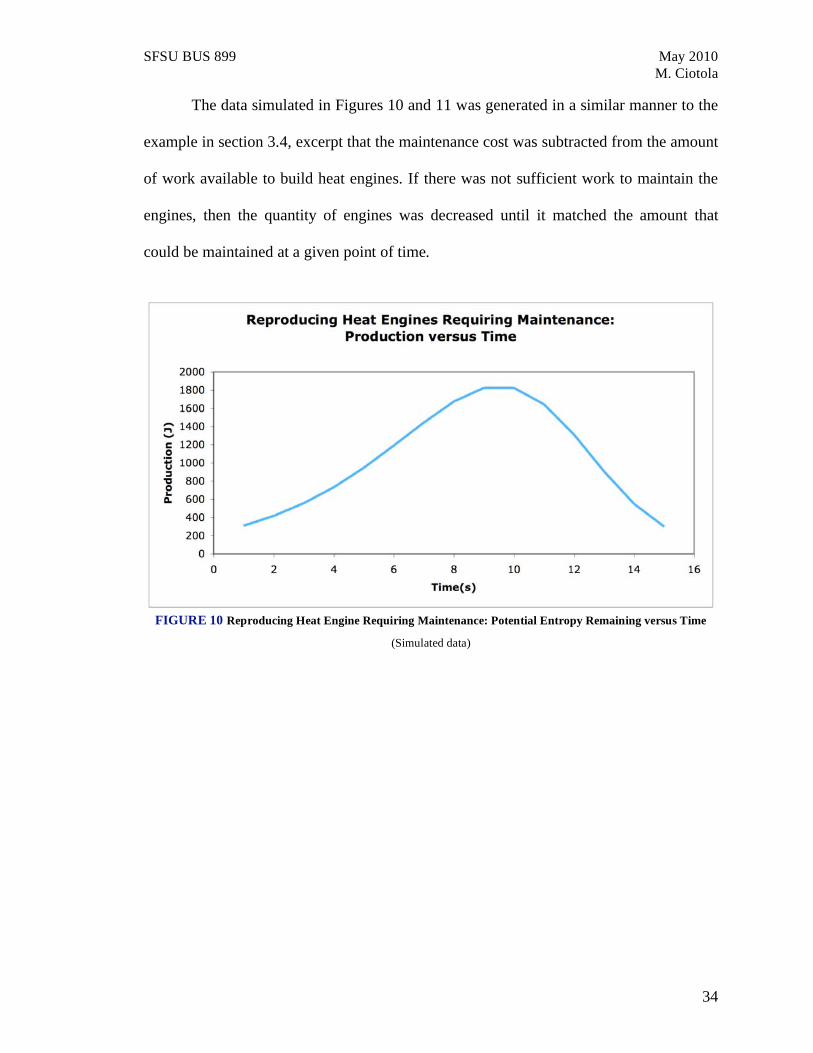
This situation is shown in Figure 10. Note that unlike the immediately above
example (shown in Figure 9), there is not dearly as steep of a drop-off of production.
However, neither is the curve symmetric. It takes longer to build up production, and less
time for it to fall at the end of the Hubbert curve.
SFSU BUS 899 May 2010
M. Ciotola
34
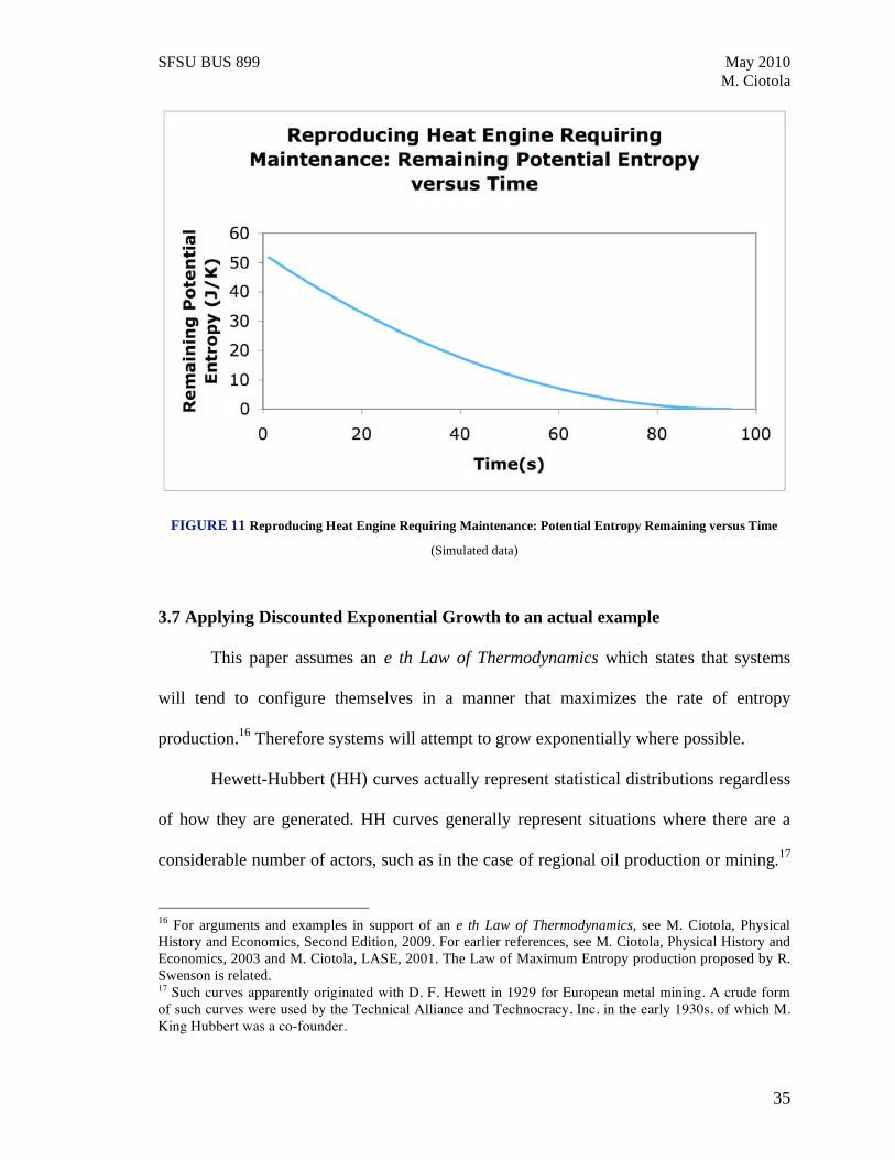
The data simulated in Figures 10 and 11 was generated in a similar manner to the
example in section 3.4, excerpt that the maintenance cost was subtracted from the amount
of work available to build heat engines. If there was not sufficient work to maintain the
engines, then the quantity of engines was decreased until it matched the amount that
could be maintained at a given point of time.
FIGURE 10 Reproducing Heat Engine Requiring Maintenance: Potential Entropy Remaining versus Time
(Simulated data)
SFSU BUS 899 May 2010
M. Ciotola
35
FIGURE 11 Reproducing Heat Engine Requiring Maintenance: Potential Entropy Remaining versus Time
(Simulated data)
3.7 Applying Discounted Exponential Growth to an actual example
This paper assumes an e th Law of Thermodynamics which states that systems
will tend to configure themselves in a manner that maximizes the rate of entropy
production.16 Therefore systems will attempt to grow exponentially where possible.
Hewett-Hubbert (HH) curves actually represent statistical distributions regardless
of how they are generated. HH curves generally represent situations where there are a
considerable number of actors, such as in the case of regional oil production or mining.17
16 For arguments and examples in support of an e th Law of Thermodynamics, see M. Ciotola, Physical History and Economics, Second Edition, 2009. For earlier references, see M. Ciotola, Physical History and
Economics, 2003 and M. Ciotola, LASE, 2001. The Law of Maximum Entropy production proposed by R.
Swenson is related. 17 Such curves apparently originated with D. F. Hewett in 1929 for European metal mining. A crude form of such curves were used by the Technical Alliance and Technocracy, Inc. in the early 1930s, of which M. King Hubbert was a co-founder.
SFSU BUS 899 May 2010
M. Ciotola
36
This allows for the formation of a Hewett-Hubbert distribution, which in turn, makes
thermodynamic modeling possible. Thermodynamic modeling is essentially a form of
statistical modeling. If there is a sufficient amount of independent actors, then an HH
curve can be modeled as a deterministic limiting case, but their statistical nature should
always be remembered.
With the e th Law in mind, we start to model an HH curve by using an pure
exponential growth function, representing output versus time. Let us call production P,
and time t, so that
P = et
In reality, there are additional multipliers (called parameters or constants), but we need
not consider those for this paper. Often, they need to be determined empirically.
However, such a function will quickly grow and approach infinity. However, in
the case of Hewett-Hubbert curves, there are limiting factors such as the amount of a
fixed resource in the ground, as well as increasing average effort needed to acquire each
additional unit of production. The rising rate of additional effort required (on average) to
produce each additional unit represents decreasing efficiency. So we need to discount
pure exponential growth by this decreasing efficiency. A simple way to do so is to
multiply the exponential growth function by efficiency. If we call efficiency d, and d is a
function of time, then
P = et D(t)
SFSU BUS 899 May 2010
M. Ciotola
37
Efficiency is itself a function of a thermodynamic potential driven by the e th
Law. Such a potential might be manifested by a vigorously sought after resource that
only exists in a limited quantity, such as in the case of a region of accessible18 gold
reserves.
A quick way19 to model efficiency is to divide cumulative production so far by the
original total amount of resource (i.e. total possible production) and subtract the result
from one. For example, if the total original amount of the resource is G and the amount
produced thus far is F, then the efficiency could be expressed as
D(t) = 1 – F(t) / G
where F is a function of time. The resulting equation is a Hewett-Hubbert curve:
P = et ( 1 – F(t) / G )
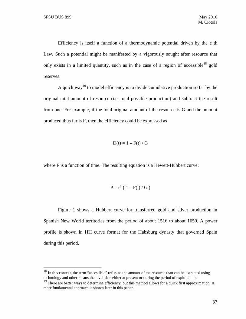
Figure 1 shows a Hubbert curve for transferred gold and silver production in
Spanish New World territories from the period of about 1516 to about 1650. A power
profile is shown in HH curve format for the Habsburg dynasty that governed Spain
during this period.
18 In this context, the term “accessible” refers to the amount of the resource than can be extracted using
technology and other means that available either at present or during the period of exploitation. 19
There are better ways to determine efficiency, but this method allows for a quick first approximation. A
more fundamental approach is shown later in this paper.
SFSU BUS 899 May 2010
M. Ciotola
38
FIGURE 1 Imports of New World Gold and Silver to 1665
(data from Gibson)
We can also generate a Hewett-Hubbert Curve directly from fundamental
thermodynamic principles, as will be shown later.
4 APPLICATION OF DISCOUNTED EXPONENTIAL APPROACH TO PETROLEUM PRODUCTION
This section will compare the strengths and weaknesses of each approach with
each other. Then both methods will be combines to determine if residuals can be further
reduced.
4.1 Regional Field Hewett-Hubbert Approach
In the early 1900s, David Foster Hewett modeled metal production in European
regions as a downward-facing curve with a peak where maximum metal production
occurred, and beginning and end-points where significant production began and ended.
SFSU BUS 899 May 2010
M. Ciotola
39
(Hewett, 1921). M. King Hubbert refined this model and applied it to petroleum
production (Hubbert, 1947, etc.). Although Hubbert was employed by Shell Oil during
much of his work, Hubbert’s approach has been viciously criticized. Most of the
objections have been political or faith-based. However, other objections have been
physical, in that Hubbert originally only counted production for the lower 48 U.S. states
and did not include Alaska, foreign source or deep-water sources. (Deffayse, etc.).
Although such arguments claim to invalidate Hubbert’s methodology, all they really do
physically is to shift the production peak to a later point of time.
4.2 Hubbert basic Formula
An initial approach to create a Hubbert formula is simply to create an inverted
parabola in the form of
y = -x2,
(Hubbert, 1980) and then fit the parabola as best as possible to the data obtained thus far.
A more sophisticated approach is to fit the data to a normal distribution such as:
y = e-t^2.
This approach works reasonably well as a first approximation. Yet uncertainly as to
where to locate the peak of the distribution can involve considerable debate and result in
SFSU BUS 899 May 2010
M. Ciotola
40
widely divergent forecasts. (See Deffeyse, 2001). Hubbert eventually developed a
somewhat different formula, but one which essentially produced a bell curve.
4.3 Discounted Exponential Growth Approach
The discounted exponential growth approach models a system as exhibiting pure
exponential growth, but then discounts that growth by a diminishing efficiency that is a
partial function of remaining potential. This approach can be modeled iteratively or
analytically.
4.4 Discounted Exponential Growth Modeled With Iterative Program
The easiest way to utilize the discounted exponential growth approach is to run
the model iteratively though a quantitative processing platform such as Microsoft Excel
or Python. This approach is demonstrated as follows. Work is calculated for each period,
and then is used to “construct” additional heat engines. (In the case of petroleum, a heat
engine could be analogous to an oil well). This process is ideally repeated until infinity,
but in practice is run until production drops below the initial level.
A Python program was written to generate the model. However, due to the limited
number of data points, the modeled was recreated using Microsoft Excel.
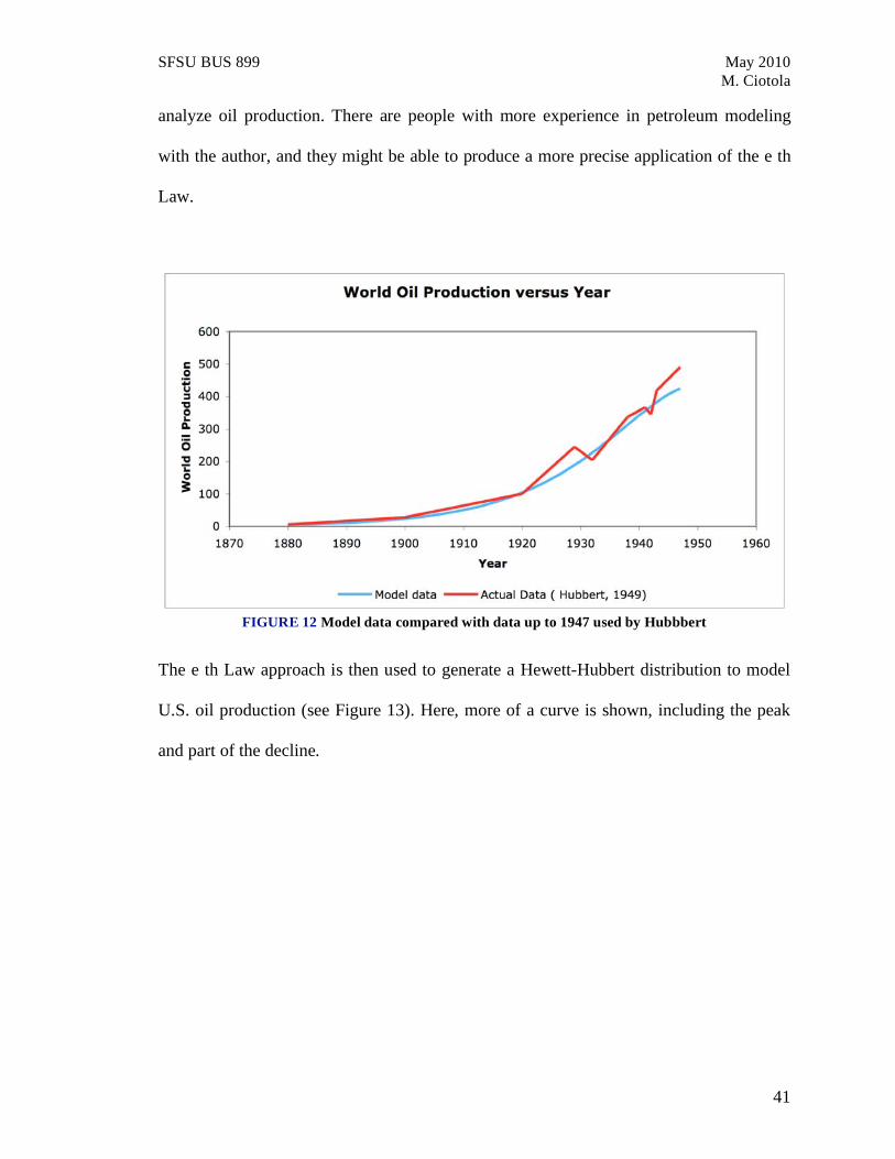
The e th Law approach is used to generate a Hewett-Hubbert distribution to model
data from M. K. Hubbert’s 1949 paper in Science magazine (see Figure 12). Here, only
the initial stages of a curve have formed, chiefly the pure exponential growth stage. Note
that this data only goes up to about 1947. The purpose of the following oil production
charts is to illustrate the general e th Law methodology and how it might be utilized to
SFSU BUS 899 May 2010
M. Ciotola
41
analyze oil production. There are people with more experience in petroleum modeling
with the author, and they might be able to produce a more precise application of the e th
Law.
FIGURE 12 Model data compared with data up to 1947 used by Hubbbert
The e th Law approach is then used to generate a Hewett-Hubbert distribution to model
U.S. oil production (see Figure 13). Here, more of a curve is shown, including the peak
and part of the decline.

SFSU BUS 899 May 2010
M. Ciotola
42
FIGURE 13 Model data compared with actual data for US Oil Production versus Year
4.5 Implementing Discounted Exponential Growth Modeled Analytically
Expressing the discounted exponential growth approach analytically is more
challenging. A simple model involving a pure exponential growth function multiplied by
a basic efficiency function is conceptually reasonable, but provides insufficient
flexibility.
The first term on the right represents pure exponential growth (e.g. see below).
The Second term on the right represents efficiency. This function successfully produces a
bell-shaped curve as shown below. For application to an actual case, appropriate
parameters in the form of constants will need to be included, such as to represent initial
conditions.
SFSU BUS 899 May 2010
M. Ciotola
43
The pure exponential growth function can be modeled either as a function of time
or of cumulative production. We will model it here as a function of cumulative
production. This term is fairly straightforward.
y = k • ex,
where k represents the initial starting condition.
4.5.1 Efficiency Term Modeled As Simple Linear Function
The simplest approach is to create efficiency as a simple linear function with a
negative slope.
y= - mx + b,
where m is the slope. Such a linear approach captures improvements in economies of
scale and better technology, thereby appropriately mitigating the initial steep drop-off of
intrinsic efficiency. A linear approach will be utilized for our model.
So we will could the following type of formula to model our approach:
y = ex mx + b( )
SFSU BUS 899 May 2010
M. Ciotola
44
Admittedly, this curve provides too steep an intersection with the x axis, but for
petroleum, that point will be of relatively little interest. For petroleum, b represents initial
efficiency, while m represents the steepness of the efficiency term. (Perhaps the
efficiency term should be replaced with the logistic equation (e.g. beginning at 1 and
ending at zero).
4.5.2 Efficiency Term Modeled In Terms of Heat Flow
The efficiency term is more challenging. We know that it starts high (but at less
than one) and ends low (but not necessarily at zero). A direct approach is:
y = 1 – (Tc/Th)
Where the difference Th - Tc represents a potential difference, or the “punch” of the
potential. Yet what are Tc and Th in the context of petroleum production? They could be
said to represent cost and benefit, respectively. Th could represent the selling price of oil,
while Tc could represent the cost of production. A high Th and low Tc would represent a
high net benefit (or, in the economics sense, “economic rent”). Th = Tc represents no net
benefit. Generally speaking, efficiency is proportionate to net benefit.
Recognizing that the reservoir temperatures may themselves be exponential
functions of the potential, then the full equation can be expressed as follows:
y =peak
parameter( )ekx 1 TcTh( ) Th+(T Th )e ( 0.001 T ( x 6)
Tc+(T Tc )e ( 0.001 T ( x 6)( )( )
SFSU BUS 899 May 2010
M. Ciotola
45
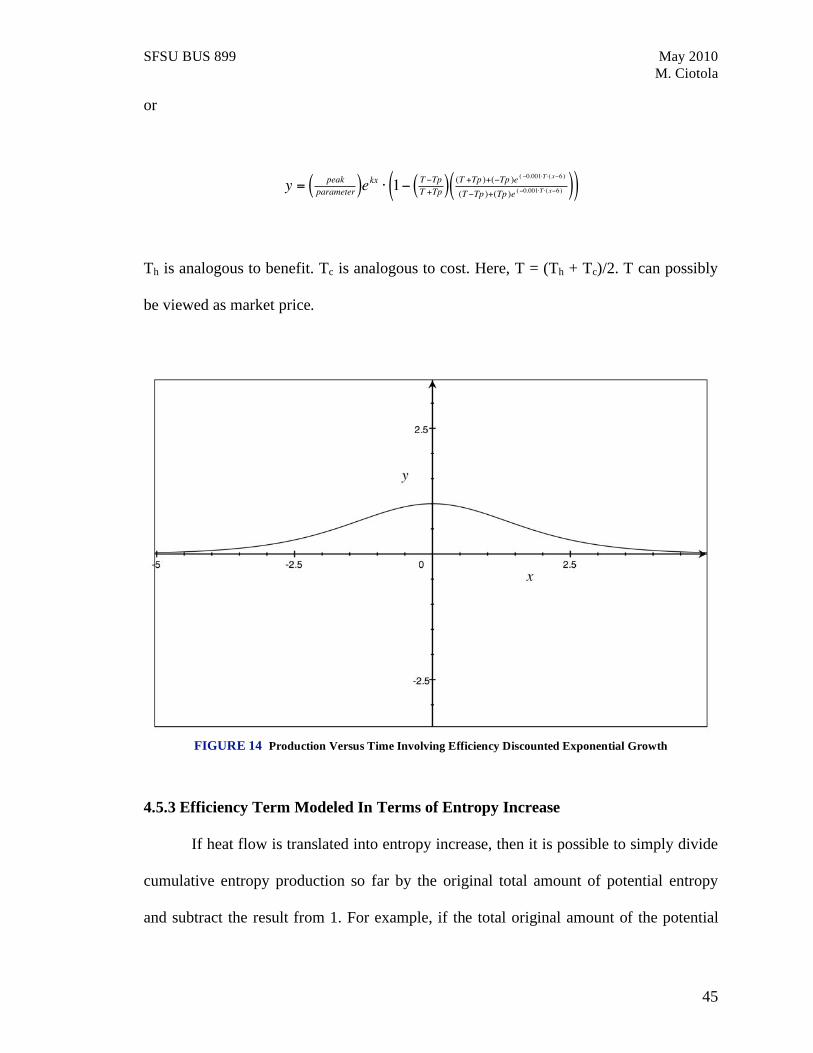
or
y =peak
parameter( )ekx 1 T TpT +Tp( ) (T +Tp )+( Tp )e ( 0.001 T ( x 6)
(T Tp )+(Tp )e ( 0.001 T ( x 6)( )( )
Th is analogous to benefit. Tc is analogous to cost. Here, T = (Th + Tc)/2. T can possibly
be viewed as market price.
FIGURE 14 Production Versus Time Involving Efficiency Discounted Exponential Growth
4.5.3 Efficiency Term Modeled In Terms of Entropy Increase
If heat flow is translated into entropy increase, then it is possible to simply divide
cumulative entropy production so far by the original total amount of potential entropy
and subtract the result from 1. For example, if the total original amount of the potential
SFSU BUS 899 May 2010
M. Ciotola
46
entropy is R0 and the amount produced thus far is St, then the efficiency could be
expressed as
E(t) = 1 – S(t) / R0
where F is a function of time. The full equation becomes:
P = et ( 1 – S(t) / R0 )
4.5.4 Comparison With Logistic Function
The above equation is similar to the logistic function:
dP/dt = P(t) ( 1 – P(t) / N )
where dP/dt represents population change with respect to time, P represents population,
and N represents a constant known as the carrying capacity. Hubbert uses the logistics
equation in part of his model (Hubbert, 1980), However, The logistics equation replaces
the exponential term with different term and does itself not produce a bell-shaped curve,
but rather approaches the constant N as t approaches infinity. This similarity suggests that
the logistics equation itself can be derived using thermodynamics.
5 COMPARISONS AND CONCLUSIONS
SFSU BUS 899 May 2010
M. Ciotola
47
This paper has shown that it is possible to generate curves that resemble Hubbert
from well-known thermodynamic principles, even if the e th Law is not fully accepted.
This approach was then used to model transferred gold and silver (analogous to
production) from Spain’s former New World territories. Application of the model gave a
fair visual fit. The thermodynamic approach provides a fundamental approach that can
then be generalized to apply to a wide range of large-scale human phenomena.
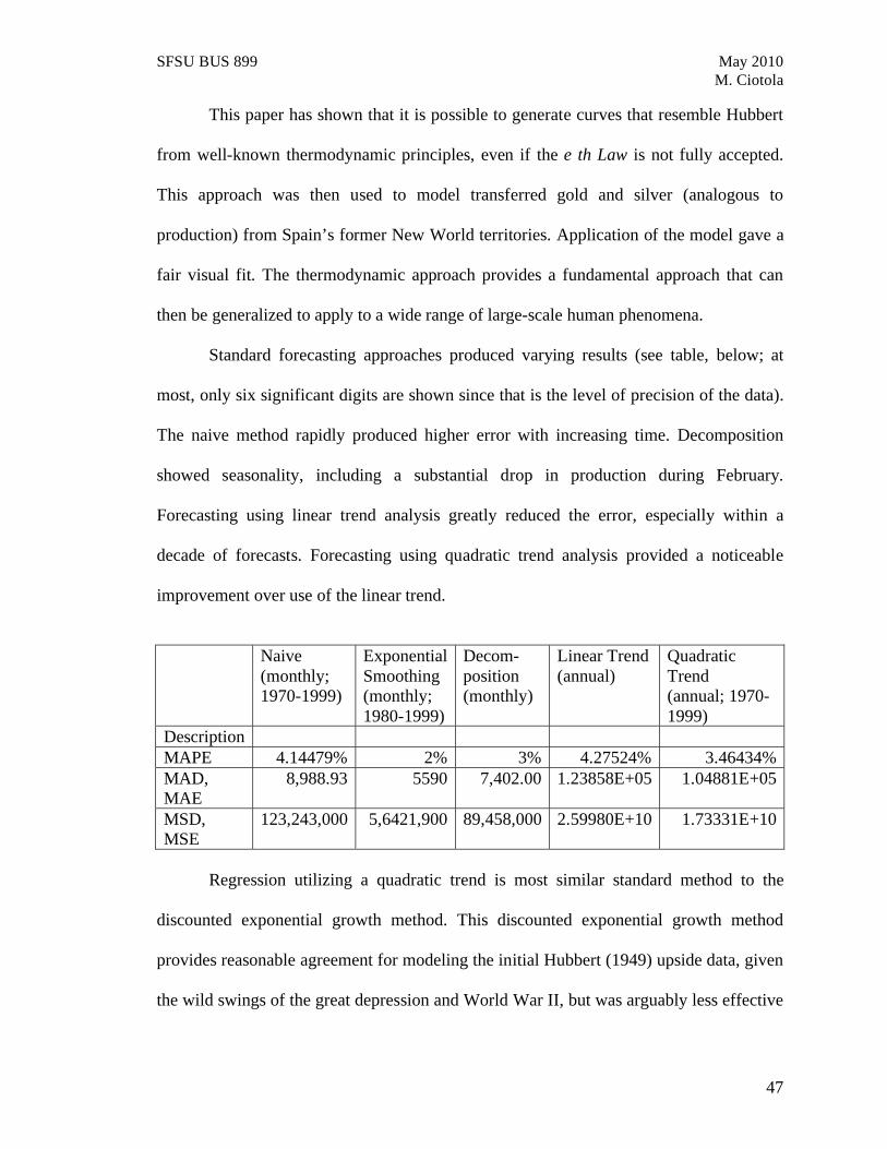
Standard forecasting approaches produced varying results (see table, below; at
most, only six significant digits are shown since that is the level of precision of the data).
The naive method rapidly produced higher error with increasing time. Decomposition
showed seasonality, including a substantial drop in production during February.
Forecasting using linear trend analysis greatly reduced the error, especially within a
decade of forecasts. Forecasting using quadratic trend analysis provided a noticeable
improvement over use of the linear trend.
Naive (monthly; 1970-1999)
Exponential Smoothing (monthly; 1980-1999)
Decom- position (monthly)
Linear Trend (annual)
Quadratic Trend (annual; 1970-1999)
Description
MAPE 4.14479% 2% 3% 4.27524% 3.46434%
MAD, MAE
8,988.93 5590 7,402.00 1.23858E+05 1.04881E+05
MSD, MSE
123,243,000 5,6421,900 89,458,000 2.59980E+10 1.73331E+10
Regression utilizing a quadratic trend is most similar standard method to the
discounted exponential growth method. This discounted exponential growth method
provides reasonable agreement for modeling the initial Hubbert (1949) upside data, given
the wild swings of the great depression and World War II, but was arguably less effective
SFSU BUS 899 May 2010
M. Ciotola
48
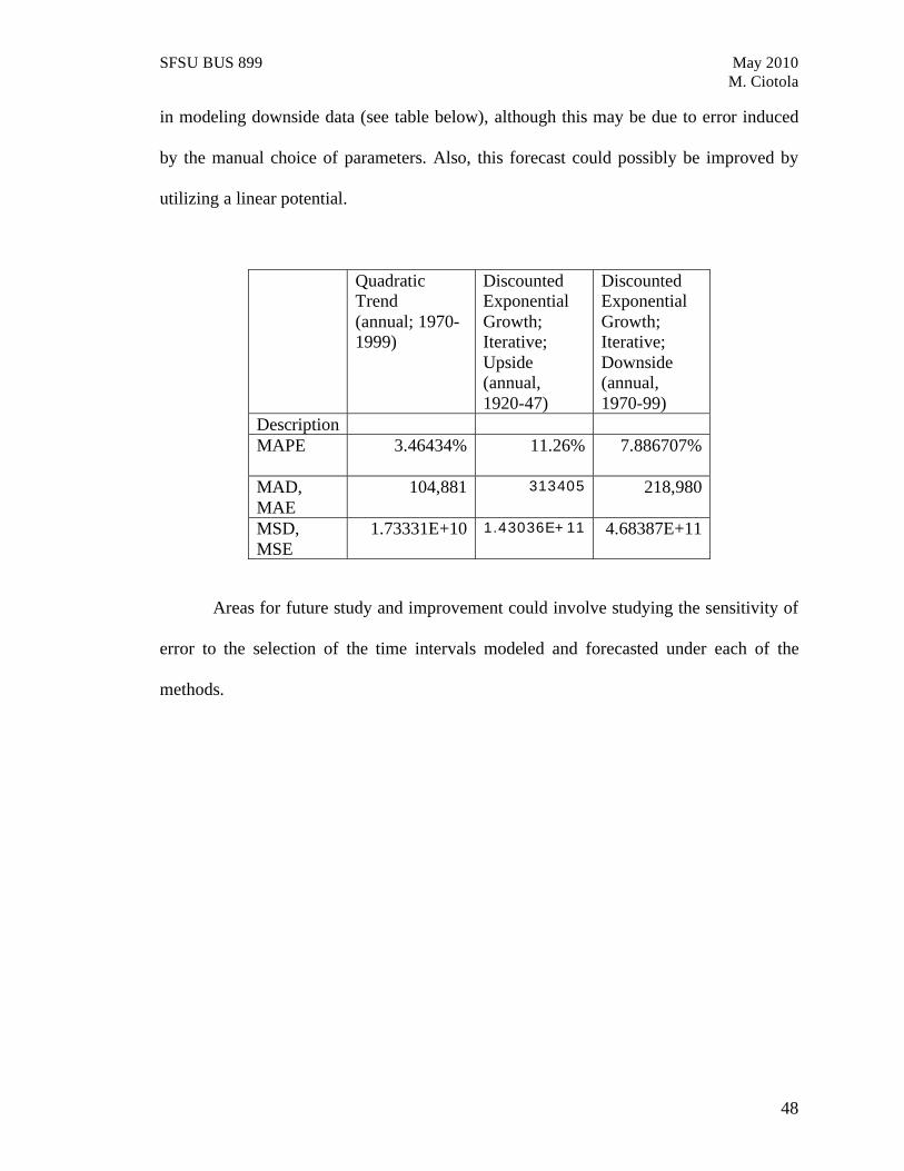
in modeling downside data (see table below), although this may be due to error induced
by the manual choice of parameters. Also, this forecast could possibly be improved by
utilizing a linear potential.
Quadratic Trend (annual; 1970-1999)
Discounted Exponential Growth; Iterative; Upside (annual, 1920-47)
Discounted Exponential Growth; Iterative; Downside (annual, 1970-99)
Description
MAPE 3.46434% 11.26% 7.886707%
MAD, MAE
104,881 313405
218,980
MSD, MSE
1.73331E+10 1.43036E+11
4.68387E+11
Areas for future study and improvement could involve studying the sensitivity of
error to the selection of the time intervals modeled and forecasted under each of the
methods.
SFSU BUS 899 May 2010
M. Ciotola
49
REFERENCES: Ahlbrandt, Thomas S. (2002), Future oil energy resources of the world. U. S. Geological Survey, Denver, CO, United States. International Geology Review. 44; 12, Pages 1092-1104. 2002. Winston & Son. Silver Spring, MD, United States. Akers, Keith (2007), The Jesus Family Tomb -- and Peak Oil. http://keithakers.com/Jesus-Family-Tomb-Peak-Oil.htm, last viewed on May 5, 2010. BBC News, "China's global hunt for oil", March 9, 2005. http://news.bbc.co.uk/2/hi/business/4191683.stm, last viewed on April 6, 2010. BBC News, "China's gets foreign oil incentives", March 1, 2007. http://news.bbc.co.uk/2/hi/business/6407337.stm, last viewed on April 6, 2010. BP (formerly British Petroleum) (2004), "Proven Oil Reserves", Geographical, 0016-741X, July 1, 2004, Vol.76, Issue 7 (which relies upon BP Statistical Review of World Energy, June 2003). Burt, J. A., "The thermal-wave lens", Can. J. Phys. 64: 1053, 198681995. Carroll, B. and D. Ostlie (2007), An Introduction to Modern Astrophysics, 2
nd Ed. Pearson Addison-Wesley.
Chapman, R.E., Oil Geology. Amsterdam: Elsevier, 1983. Ciotola, M. (1997), "San Juan Mining Region Case Study: Application of Maxwell-Boltzmann Distribution Function", Journal of Physical History and Economics, Vol 1. Ciotola, M. (2001), "Factors Affecting Calculation of L", Kingsley, S., R. Bhathal, ed.s, Conference Proceedings, International Society for Optical Engineering (SPIE), Vol. 4273. Ciotola, M. (2002), Hurtling Towards Heat Death (talk delivered at San Francisco State University). September,. Ciotola, M. (2003), Physical History and Economics. Pavilion Press, San Francisco. Ciotola, M. (2006), "Thermodynamic Perspective on Profits", North American Technocrat, Vol. 5, Issue 18. Deffeyes, Kenneth S. (2001), Hubbert's Peak. Princeton: Princeton University Press. Energy Information Administration, U.S. Oil Production figures, 2009, 2010. Energy Information Administration, World Petroleum Consumption, Annual Estimates, 1980-2008, 2009. Energy Information Administration, International Energy Outlook 2004. Energy Information Administration, February 2010 International Petroleum Monthly, March 10, 2010.
SFSU BUS 899 May 2010
M. Ciotola
50
Energy Information Administration, Short-Term Energy Outlook, March 8, 2005. Energy Information Administration, Petroleum Marketing Annual 2003. Energy Information Administration, Oil and Gas Supply Module Documentation, 2004. Energy Information Administration, World Proved Crude Oil Reserves, 2009. Garraty J. A. and P. Gay (1972), Columbia History of the World. Dorset Press (Harper and Rowe). Georgescu-Roegen, N. (1971), The Entropy Law and the Economic Process. Harvard University Press. Gibson, C. (1966), Spain in America. Harper and Row. Hanke, John E., Wichern, Dean W. (2005), Business Forecasting, 8
th Ed. Prentice Hall.
Heilbroner, R. L. (1980), The Worldly Philosophers 5
th Ed. (Touchstone (Simon and Schuster).
Hewett, D. F. (1929), Cycles in Metal Production, Technical Publication 183. The American Institute of of Mining and Metallurgical Engineers. Hubbert, M. K. (1936), "Man-Hours and Distribution", Technocracy. Series A, No. 8. Hubbert, M. K. (1947), "Energy from Fossil Fuels", Science. Vol. 109. Hubbert, M. King, 1980. J. Lunine, (2005), Astrobiology, A Multidisciplinary Approach. Pearson Addison Wesley. Mazour, A. G., and J. M. Peoples (1975), Men and Nations, A World History, 3
rd Ed., Harcourt, Brace, Jovanovich.
Meadows, D, and D. Meadows, J. Randers and W. Behrens III (1972), Limits to Growth, Club of Rome. Prigogine, I. (1967), Introduction to Thermodynamics of Irreversible Processes, Wiley, New York, pp. 67. ff. Riva, Joseph P. (1983), World Oil and Reserves, Boulder, Colorado: Westview Press, Inc. Schroeder, D. V. (2000), Introduction to Thermal Physics. Addison Wesley Longman. Stowe, K. (1984), Introduction to Statistical Mechanics and Thermodynamics. John Wiley & Sons. United States Geological Survey, 2010, etc. Note on references:

SFSU BUS 899 May 2010
M. Ciotola
51
The author independently conceived the statements made in this essay, with the exceptions, of course, of the 1st and 2nd Laws of Thermodynamics and its application to heat engines, and Hubbert’s peak production hypothesis. However, so many people have written on thermodynamics, that the author does not claim the statements are new. Nevertheless, to the author’s knowledge, the author is the first to synthesize all of these statements into an integrated whole. The author has subsequently been introduced to relevant the prior work of R. Swenson and I. Prigogine who have themselves discovered some of the major pieces.
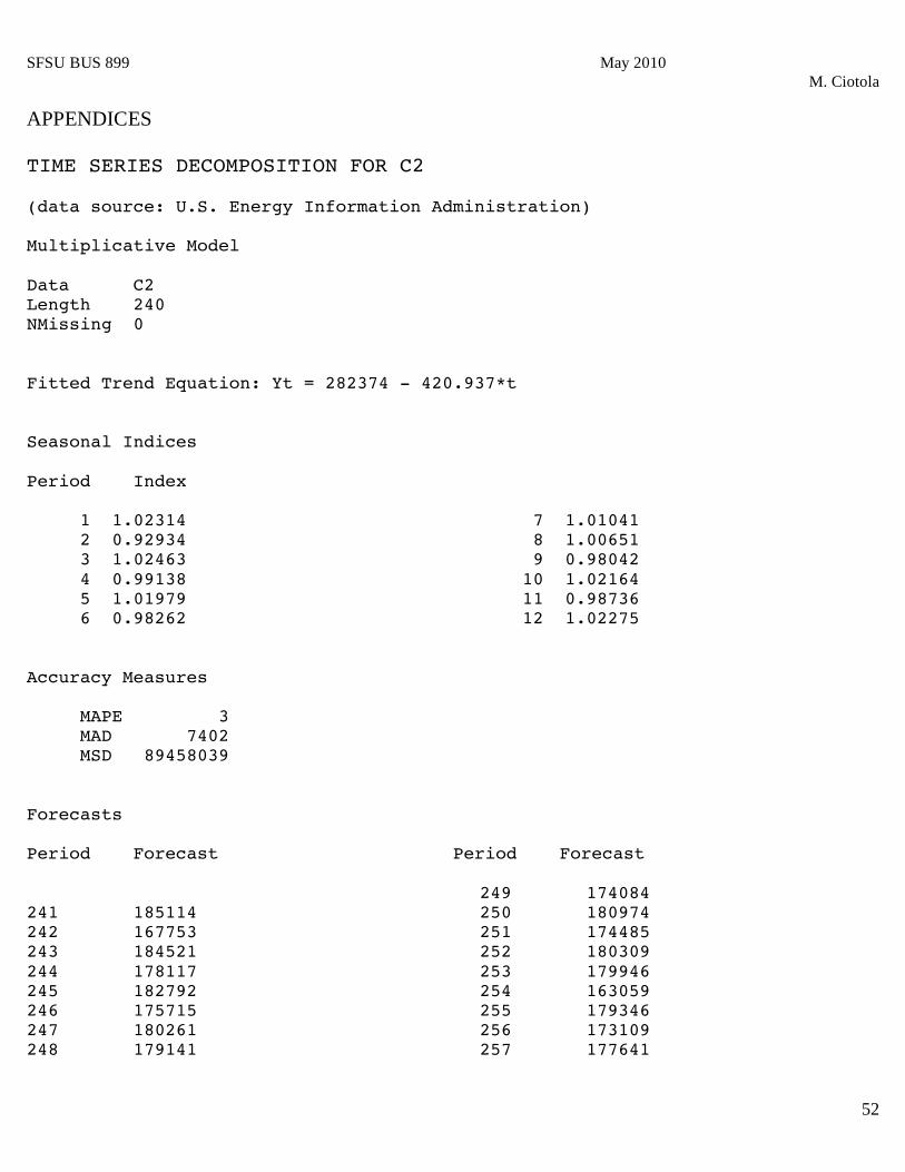
SFSU BUS 899 May 2010
M. Ciotola
52
APPENDICES TIME SERIES DECOMPOSITION FOR C2 (data source: U.S. Energy Information Administration) Multiplicative Model Data C2 Length 240 NMissing 0 Fitted Trend Equation: Yt = 282374 - 420.937*t Seasonal Indices Period Index 1 1.02314 2 0.92934 3 1.02463 4 0.99138 5 1.01979 6 0.98262
7 1.01041 8 1.00651 9 0.98042 10 1.02164 11 0.98736 12 1.02275
Accuracy Measures
MAPE 3 MAD 7402 MSD 89458039
Forecasts Period Forecast Period Forecast 241 185114 242 167753 243 184521 244 178117 245 182792 246 175715 247 180261 248 179141
249 174084 250 180974 251 174485 252 180309 253 179946 254 163059 255 179346 256 173109 257 177641
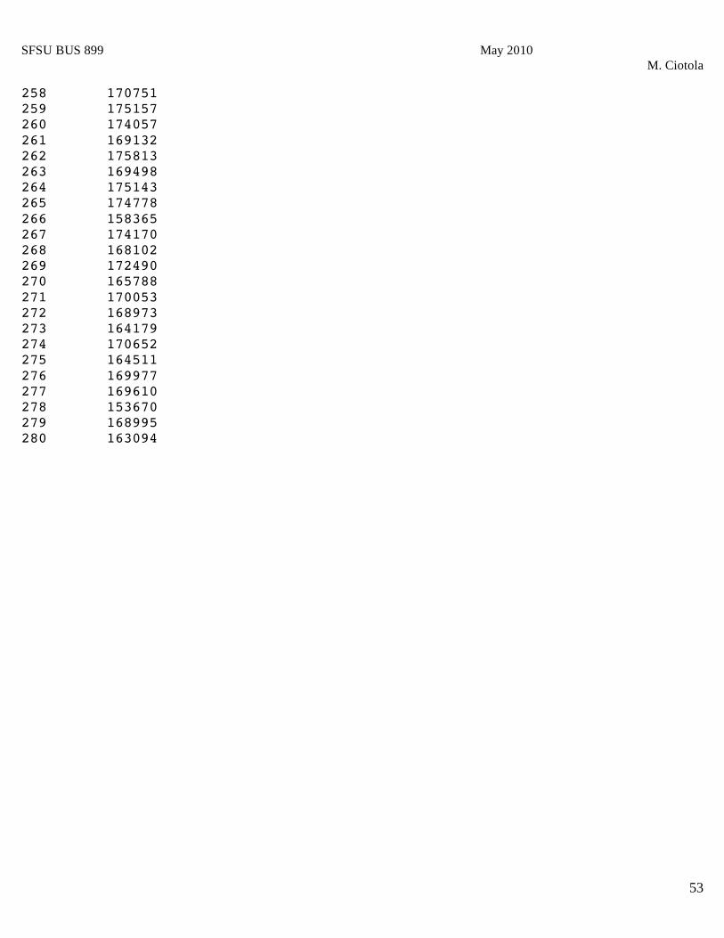
SFSU BUS 899 May 2010
M. Ciotola
53
258 170751 259 175157 260 174057 261 169132 262 175813 263 169498 264 175143 265 174778 266 158365 267 174170 268 168102 269 172490 270 165788 271 170053 272 168973 273 164179 274 170652 275 164511 276 169977 277 169610 278 153670 279 168995 280 163094
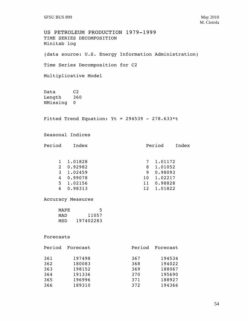
SFSU BUS 899 May 2010
M. Ciotola
54
US PETROLEUM PRODUCTION 1979-1999 TIME SERIES DECOMPOSITION Minitab log (data source: U.S. Energy Information Administration) Time Series Decomposition for C2 Multiplicative Model Data C2 Length 360 NMissing 0 Fitted Trend Equation: Yt = 294539 - 278.633*t Seasonal Indices Period Index Period Index
1 1.01828 2 0.92982 3 1.02459 4 0.99078 5 1.02156 6 0.98313
7 1.01172 8 1.01052 9 0.98093 10 1.02217 11 0.98828 12 1.01822
Accuracy Measures
MAPE 5 MAD 11057 MSD 197402283
Forecasts Period Forecast Period Forecast 361 197498 362 180083 363 198152 364 191336 365 196996 366 189310
367 194534 368 194022 369 188067 370 195690 371 188927 372 194366
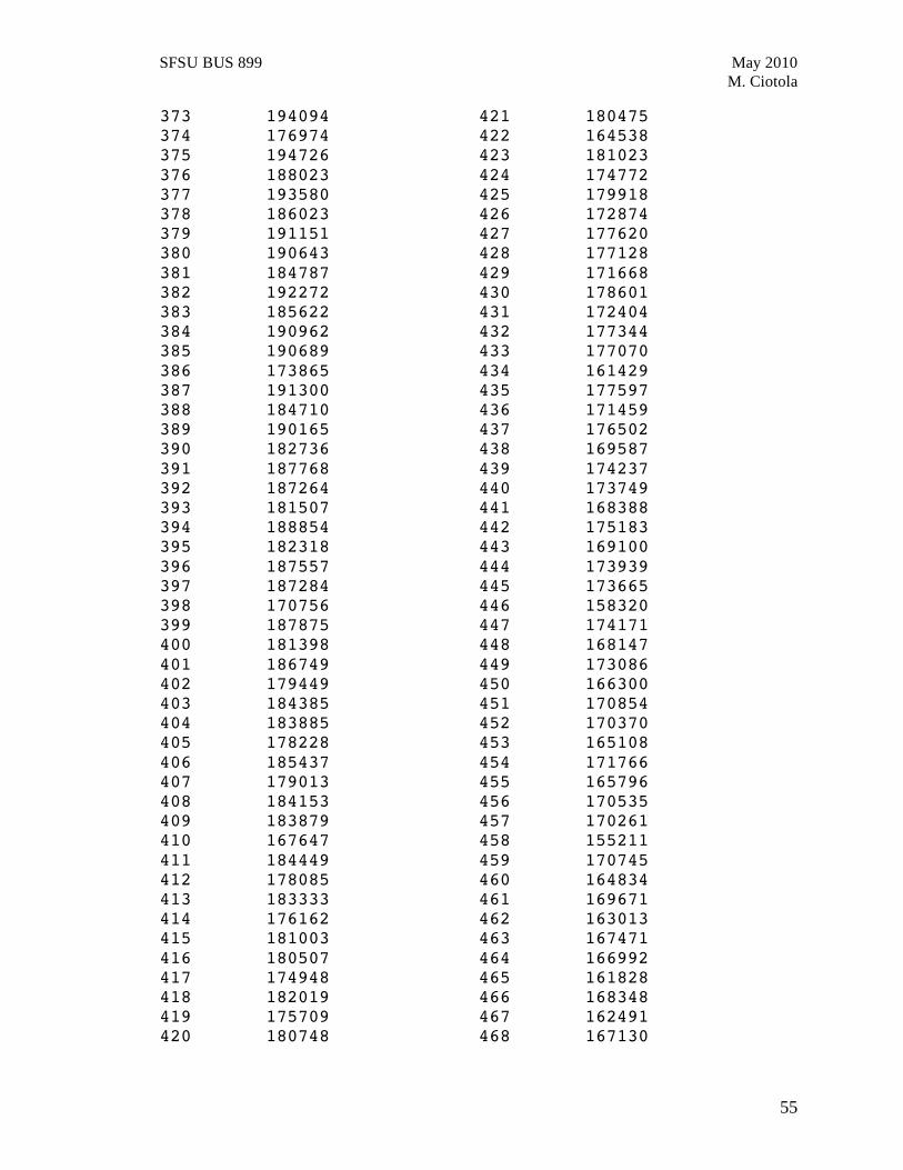
SFSU BUS 899 May 2010
M. Ciotola
55
373 194094 374 176974 375 194726 376 188023 377 193580 378 186023 379 191151 380 190643 381 184787 382 192272 383 185622 384 190962 385 190689 386 173865 387 191300 388 184710 389 190165 390 182736 391 187768 392 187264 393 181507 394 188854 395 182318 396 187557 397 187284 398 170756 399 187875 400 181398 401 186749 402 179449 403 184385 404 183885 405 178228 406 185437 407 179013 408 184153 409 183879 410 167647 411 184449 412 178085 413 183333 414 176162 415 181003 416 180507 417 174948 418 182019 419 175709 420 180748
421 180475 422 164538 423 181023 424 174772 425 179918 426 172874 427 177620 428 177128 429 171668 430 178601 431 172404 432 177344 433 177070 434 161429 435 177597 436 171459 437 176502 438 169587 439 174237 440 173749 441 168388 442 175183 443 169100 444 173939 445 173665 446 158320 447 174171 448 168147 449 173086 450 166300 451 170854 452 170370 453 165108 454 171766 455 165796 456 170535 457 170261 458 155211 459 170745 460 164834 461 169671 462 163013 463 167471 464 166992 465 161828 466 168348 467 162491 468 167130
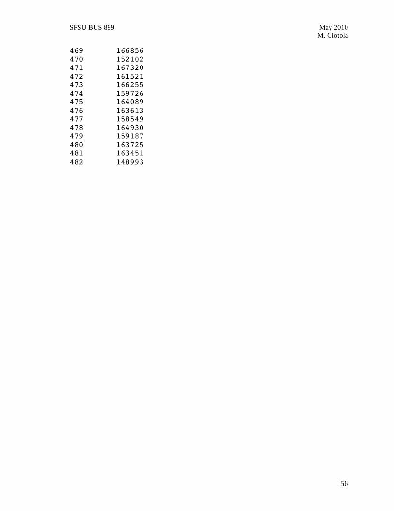
SFSU BUS 899 May 2010
M. Ciotola
56
469 166856 470 152102 471 167320 472 161521 473 166255 474 159726 475 164089 476 163613 477 158549 478 164930 479 159187 480 163725 481 163451 482 148993
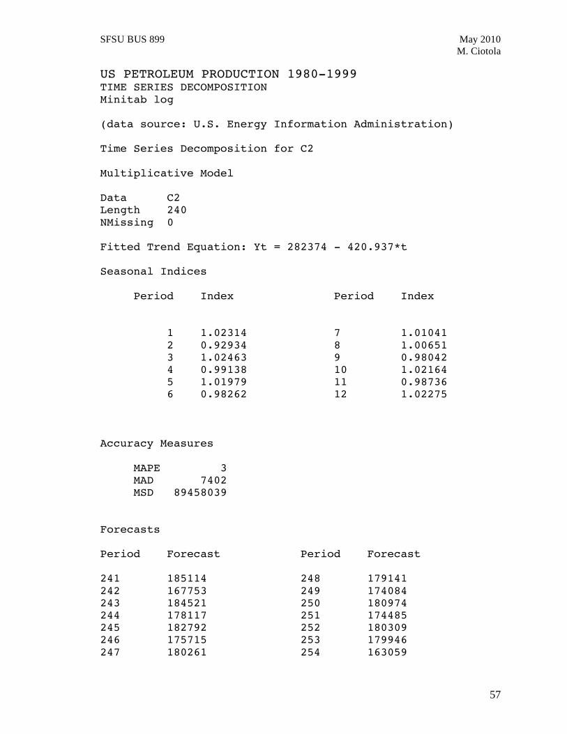
SFSU BUS 899 May 2010
M. Ciotola
57
US PETROLEUM PRODUCTION 1980-1999 TIME SERIES DECOMPOSITION Minitab log (data source: U.S. Energy Information Administration) Time Series Decomposition for C2 Multiplicative Model Data C2 Length 240 NMissing 0 Fitted Trend Equation: Yt = 282374 - 420.937*t Seasonal Indices
Period Index Period Index
1 1.02314
2 0.92934 3 1.02463 4 0.99138 5 1.01979 6 0.98262
7 1.01041 8 1.00651 9 0.98042 10 1.02164 11 0.98736 12 1.02275
Accuracy Measures
MAPE 3 MAD 7402 MSD 89458039
Forecasts Period Forecast Period Forecast 241 185114 242 167753 243 184521 244 178117 245 182792 246 175715 247 180261
248 179141 249 174084 250 180974 251 174485 252 180309 253 179946 254 163059
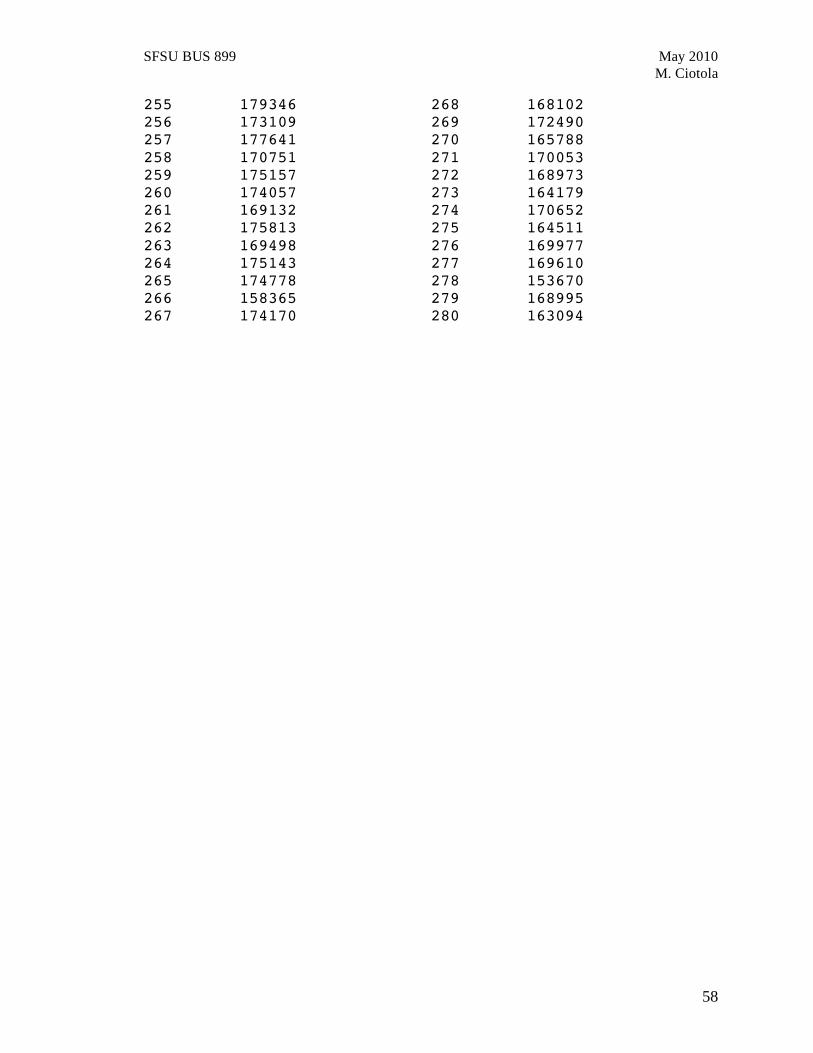
SFSU BUS 899 May 2010
M. Ciotola
58
255 179346 256 173109 257 177641 258 170751 259 175157 260 174057 261 169132 262 175813 263 169498 264 175143 265 174778 266 158365 267 174170
268 168102 269 172490 270 165788 271 170053 272 168973 273 164179 274 170652 275 164511 276 169977 277 169610 278 153670 279 168995 280 163094
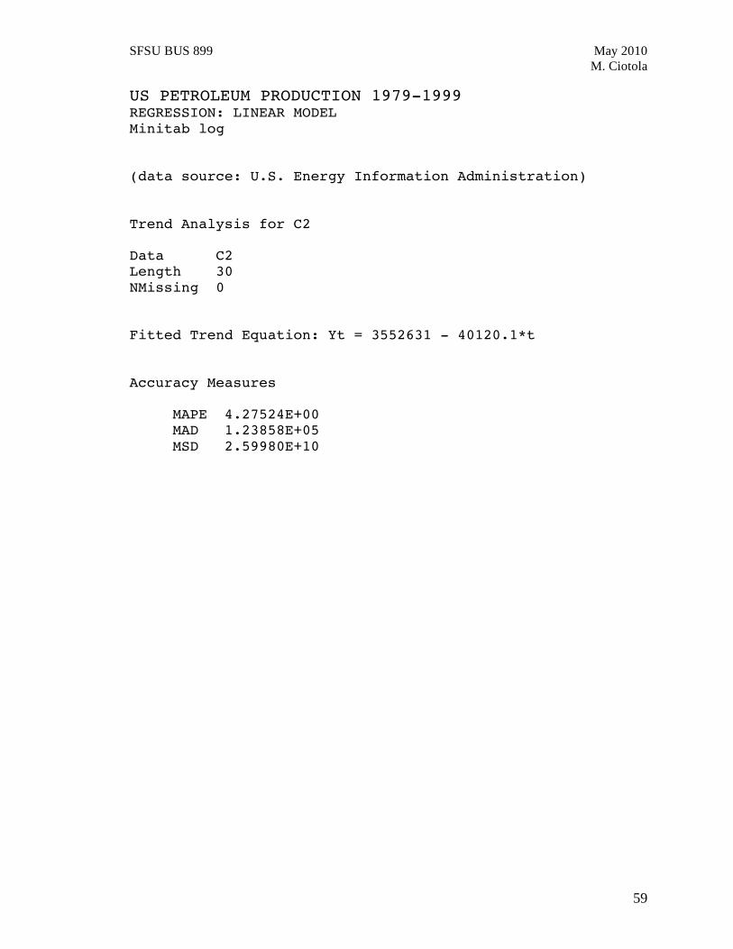
SFSU BUS 899 May 2010
M. Ciotola
59
US PETROLEUM PRODUCTION 1979-1999 REGRESSION: LINEAR MODEL Minitab log (data source: U.S. Energy Information Administration) Trend Analysis for C2 Data C2 Length 30 NMissing 0 Fitted Trend Equation: Yt = 3552631 - 40120.1*t Accuracy Measures
MAPE 4.27524E+00 MAD 1.23858E+05 MSD 2.59980E+10
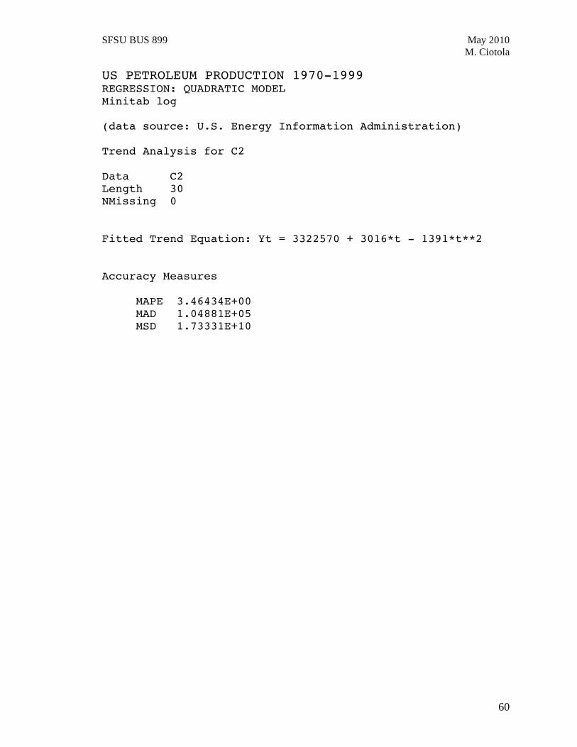
SFSU BUS 899 May 2010
M. Ciotola
60
US PETROLEUM PRODUCTION 1970-1999 REGRESSION: QUADRATIC MODEL Minitab log (data source: U.S. Energy Information Administration) Trend Analysis for C2 Data C2 Length 30 NMissing 0 Fitted Trend Equation: Yt = 3322570 + 3016*t - 1391*t**2 Accuracy Measures
MAPE 3.46434E+00 MAD 1.04881E+05 MSD 1.73331E+10
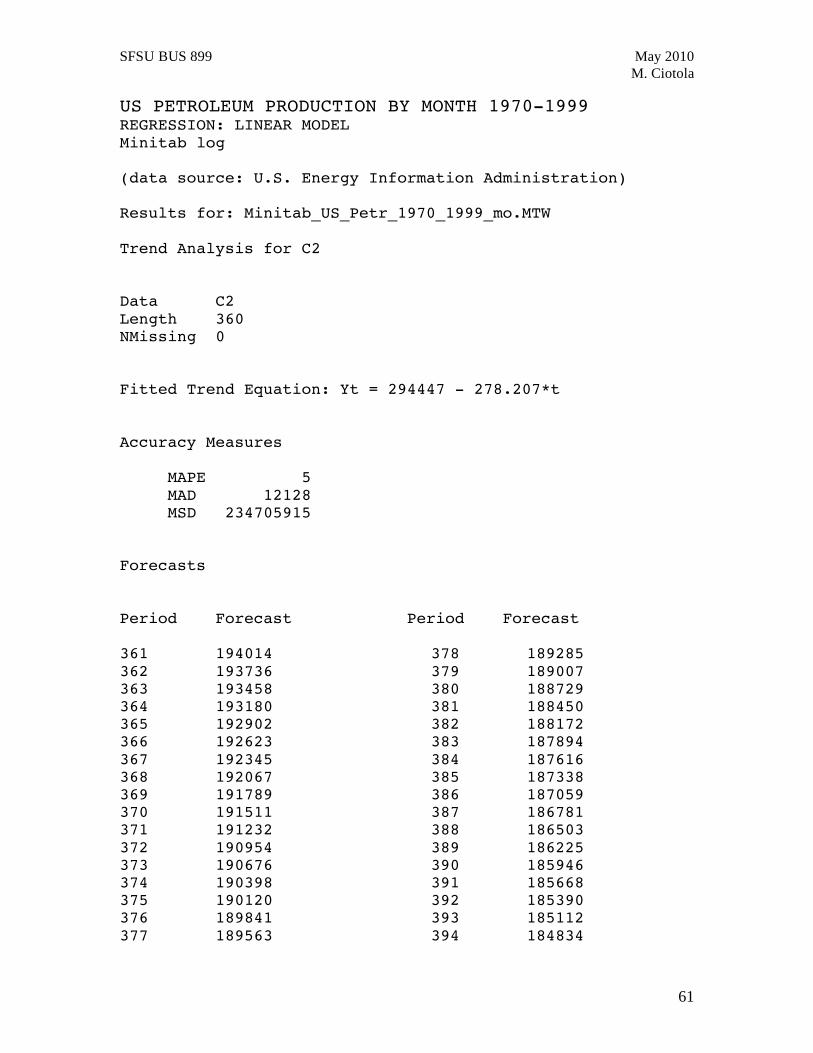
SFSU BUS 899 May 2010
M. Ciotola
61
US PETROLEUM PRODUCTION BY MONTH 1970-1999 REGRESSION: LINEAR MODEL Minitab log (data source: U.S. Energy Information Administration) Results for: Minitab_US_Petr_1970_1999_mo.MTW Trend Analysis for C2 Data C2 Length 360 NMissing 0 Fitted Trend Equation: Yt = 294447 - 278.207*t Accuracy Measures
MAPE 5 MAD 12128 MSD 234705915
Forecasts Period Forecast Period Forecast 361 194014 362 193736 363 193458 364 193180 365 192902 366 192623 367 192345 368 192067 369 191789 370 191511 371 191232 372 190954 373 190676 374 190398 375 190120 376 189841 377 189563
378 189285 379 189007 380 188729 381 188450 382 188172 383 187894 384 187616 385 187338 386 187059 387 186781 388 186503 389 186225 390 185946 391 185668 392 185390 393 185112 394 184834

SFSU BUS 899 May 2010
M. Ciotola
62
395 184555 396 184277 397 183999 398 183721 399 183443 400 183164
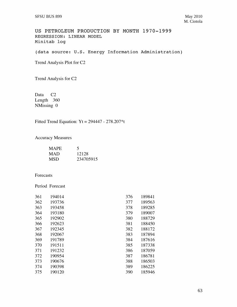
SFSU BUS 899 May 2010
M. Ciotola
63
US PETROLEUM PRODUCTION BY MONTH 1970-1999 REGRESSION: LINEAR MODEL Minitab log (data source: U.S. Energy Information Administration) Trend Analysis Plot for C2 Trend Analysis for C2 Data C2 Length 360 NMissing 0 Fitted Trend Equation: Yt = 294447 - 278.207*t Accuracy Measures
MAPE 5 MAD 12128 MSD 234705915
Forecasts Period Forecast 361 194014 362 193736 363 193458 364 193180 365 192902 366 192623 367 192345 368 192067 369 191789 370 191511 371 191232 372 190954 373 190676 374 190398 375 190120
376 189841 377 189563 378 189285 379 189007 380 188729 381 188450 382 188172 383 187894 384 187616 385 187338 386 187059 387 186781 388 186503 389 186225 390 185946
SFSU BUS 899 May 2010
M. Ciotola
64
391 185668 392 185390 393 185112 394 184834 395 184555 396 184277 397 183999 398 183721 399 183443 400 183164 401 182886 402 182608 403 182330 404 182052 405 181773 406 181495 407 181217 408 180939 409 180661 410 180382 411 180104 412 179826 413 179548 414 179270 415 178991 416 178713 417 178435 418 178157 419 177878 420 177600 421 177322 422 177044 423 176766 424 176487 425 176209 426 175931 427 175653 428 175375 429 175096 430 174818 431 174540 432 174262 433 173984 434 173705 435 173427 436 173149
437 172871 438 172593 439 172314 440 172036 441 171758 442 171480 443 171202 444 170923 445 170645 446 170367 447 170089 448 169810 449 169532 450 169254 451 168976 452 168698 453 168419 454 168141 455 167863 456 167585 457 167307 458 167028 459 166750 460 166472 461 166194 462 165916 463 165637 464 165359 465 165081 466 164803 467 164525 468 164246 469 163968 470 163690 471 163412 472 163134 473 162855 474 162577 475 162299 476 162021 477 161742 478 161464 479 161186 480 160908 481 160630 482 160351

SFSU BUS 899 May 2010
M. Ciotola
65
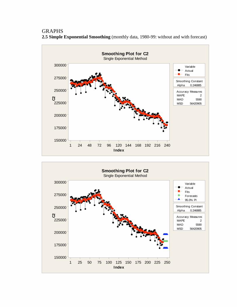
GRAPHS 2.5 Simple Exponential Smoothing (monthly data, 1980-99: without and with forecast)
240216192168144120967248241
300000
275000
250000
225000
200000
175000
150000
Index
C2
Alpha 0.246885
Smoothing Constant
MAPE 2
MAD 5590
MSD 56420905
Accuracy Measures
Actual
Fits
Variable
Smoothing Plot for C2Single Exponential Method
2502252001751501251007550251
300000
275000
250000
225000
200000
175000
150000
Index
C2
Alpha 0.246885
Smoothing Constant
MAPE 2
MAD 5590
MSD 56420905
Accuracy Measures
Actual
Fits
Forecasts
95.0% PI
Variable
Smoothing Plot for C2Single Exponential Method
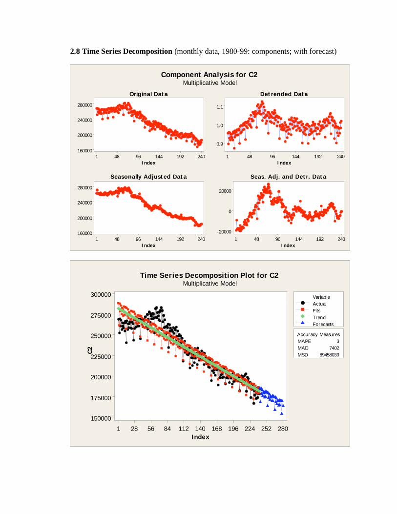
2.8 Time Series Decomposition (monthly data, 1980-99: components; with forecast)
24019214496481
280000
240000
200000
160000
Index
24019214496481
280000
240000
200000
160000
Index
24019214496481
1.1
1.0
0.9
Index
24019214496481
20000
0
-20000
Index
Component Analysis for C2Multiplicative Model
Original Data
Seasonally Adjusted Data
Detrended Data
Seas. Adj. and Detr. Data
2802522241961681401128456281
300000
275000
250000
225000
200000
175000
150000
Index
C2
MAPE 3
MAD 7402
MSD 89458039
Accuracy Measures
Actual
Fits
Trend
Forecasts
Variable
Time Series Decomposition Plot for C2Multiplicative Model
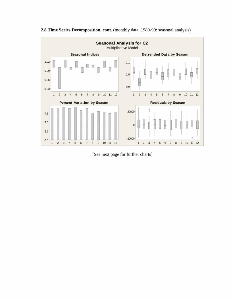
2.8 Time Series Decomposition, cont. (monthly data, 1980-99: seasonal analysis)
121110987654321
1.02
0.99
0.96
0.93
121110987654321
7.5
5.0
2.5
0.0
121110987654321
1.1
1.0
0.9
121110987654321
20000
0
-20000
Seasonal Analysis for C2Multiplicative Model
Seasonal Indices
Percent Variation by Season
Detrended Data by Season
Residuals by Season
[See next page for further charts]
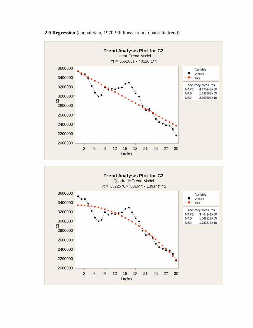
2.9 Regression (annual data, 1970-99: linear trend; quadratic trend)
30272421181512963
3600000
3400000
3200000
3000000
2800000
2600000
2400000
2200000
2000000
Index
C2
MAPE 4.27524E+00
MAD 1.23858E+05
MSD 2.59980E+10
Accuracy Measures
Actual
Fits
Variable
Trend Analysis Plot for C2Linear Trend Model
Yt = 3552631 - 40120.1*t
30272421181512963
3600000
3400000
3200000
3000000
2800000
2600000
2400000
2200000
2000000
Index
C2
MAPE 3.46434E+00
MAD 1.04881E+05
MSD 1.73331E+10
Accuracy Measures
Actual
Fits
Variable
Trend Analysis Plot for C2Quadratic Trend Model
Yt = 3322570 + 3016*t - 1391*t**2