terminal value calculations with the discounted cash flow
TRANSCRIPT

Terminal value calculations with the Discounted
Cash Flow model
Differences between literature and practice
University of Twente
Faculty of Behavioural, Management and Social Sciences
Supervision:
Ir. H Kroon
Dr. P.C. Schuur
Master in Business Administration
Master Thesis
Tim ten Beitel
S1665987
June 2016

Terminal Value Calculations with DCF
2
Preface
This thesis was written as a final task in the Master of Business Administration at the University of
Twente. Within this master I have been challenged on multiple areas of business administration and
the financial courses stood out for me. The interest I had in especially corporate and entrepreneurial
finance made it logical to choose a topic within these courses. The elusive side of valuation was
decisive for me to choose this interesting subject to focus upon.
In this I would like to thank my supervisors at the university for advising and guiding me. Especially
Henk Kroon who has been my teacher during one of the courses. He stood out as an unconventional
but therefore in my eyes a much better teacher. This is why I wanted him as a supervisor for this
project, in which he created a good starting point followed by a positive process. I would like to also
thank the respondents who have helped me with their time and provided me with the valuable
information needed to complete this thesis. At last I thank my parents for their support and
encouragement to both start and finish this Master.
Tim ten Beitel
Terminal Value Calculations with DCF
3
Abstract
This thesis has as goal to gain an insight in the differences in literature and practice regarding the use
of the Discounted Cash Flow method in valuation. The popularity of the method does not imply that
literature is in agreement over the most suitable calculation for especially the terminal period during
valuation.
The aim of this thesis is to find an answer to the research question;” To what extend differs practice
from current literature in terminal value calculations for DCF valuations of SME’s”. The focus in this
lies on the focus points and driving factors for authors to improve this model, and the discrepancy
between this and the selecting criteria for practitioners. The contributing factor of this to literature
has multiple sides to it. Firstly, by providing an overview of the different methods designed.
Secondly, by gaining an insight in the different focus points between literature and practice. And
thirdly by providing an opinion in whether and how these differences could be approached.
The design of the research could be described as a qualitative study with input from practitioners in
the field of valuation. Real life valuation reports together with semi-structured interviews serve as
the source out of which the data could be analyzed and from which conclusions on practitioners’
points of view can be drawn. The driving factors behind literature improvement in terminal value
calculation could be stated as follows: a) an increase in consistency, b) an improvement of
transparency, c) the natural pattern of growth rates and d) the better understanding of market
analysis. The criteria for practitioners in the selection of the most suitable terminal value method
are: a) the dependency towards clients and key management, b) the degree of attribution to current
owners, c) the feasibility of the deal in the takeover, and d) the ability to fund this deal. The main
finding in this is that the evolution of methods in literature have a value-enhancing effect whereas
the criteria for practitioners result in a more conservative approach.
This study is limited due to the sample size and qualitative design of the study. These make it hard to
provide a generalizable conclusion. Therefore the reliability of the results should be placed into
perspective.
Terminal Value Calculations with DCF
4
Table of Contents
Preface 2
Abstract 3
List of abbreviations 6
List of formulas, tables and figures 7
1 Introduction 8
1.1 Valuation 8
1.2 Research Question 8
1.3 Contributions 10
1.4 Approach and Outline 11
2 Theoretical Framework 12
2.1 Discounted Cash Flow Model 12
2.2 Terminal value approaches 17
2.3 Relative importance of the Terminal Value on total Value 21
2.4 Growth Patterns in DCF Terminal Value Calculations 22
2.5 Conclusions of the Theoretical Framework 24
3 Methodology 25
3.1 Introduction 25
3.2 Research Design 25
3.3 Collection and Analysis 26
Terminal Value Calculations with DCF
5
4 Results 29
4.1 Introduction 29
4.2 Focus in Literature on Terminal Value Calculations 29
4.3 Focus of Practitioners on Terminal Value Calculations 33
4.4 How to approach differences between Literature and Practice 37
5 Conclusion 38
6 Discussion, implications, limitations and future research 40
References 42
Appendix I Formulas 45
Appendix II Tables 47
Appendix III Interview questions 48
Terminal Value Calculations with DCF
6
List of Abbreviations
APV Adjusted Present Value
CAPEX Capital Expenditures
CAPM Capital Asset Pricing Model
CCF Capital Cash Flow
CVA Cash Value Added
CFROI Cash Flow Return On Investment
DCF Discounted Cash Flow
DDM Dividend Discount Model
EBIT Earnings Before Interest and Taxes
EBITDA Earnings Before Interest and Taxes, Depreciation and Amortization
ECF Equity Cash Flow
EVA Economic Value Added
EP Economic Profit
FCF Free Cash Flow
FCFE Free Cash Flow to Equity
FCFF Free Cash Flow to Firm
GDP Gross Domestic Product
NOPAT Net Operating Profit After Taxes
NPV Net Present Value
NWC Net Working Capital
RONIC Return on newly invested capital
SME Small and Medium Enterprises
TV Terminal Value
WACC Weighted Average Cost of Capital
Terminal Value Calculations with DCF
7
List of Formulas, Tables and Figures
Formulas
Formula1: DCF Net Present Value (Brealey , Myers, Allen., 2010)……………………………………………………12
Formula 2: Cost of Debt (Palepu, Healy, Peek., 2013)………………………………………………………………………14
Formula 3: Cost of Equity (Sharpe., 1964)………………………………………………………………………………………..14
Formula 4: Weighted Average Cost of Capital a (Brealey et al., 2010)……………………………………………..15
Formula 5: Weighted Average Cost of Capital b (Palepu et al., 2013)……………………………………………..15
Formula 6: Terminal Value Basic Perpetuity…………………………………………………………………………………….18
Formula 7: Terminal Value Gordon growth formula (Gordon., 1959)……………………………………………..18
Formula 8: Terminal Value Koller Value Driver Formula (Koller, Goedhart, Wessels., 2010)………….19
Formula 9: Terminal Value Koller Two-stage Value Driver Formula (Koller et al. 2010)………………….19
Formula 10: Terminal Value The Three-stage TV model (Damodaran. 2012)………………………………….20
Tables
Table 1: Degree of fulfillment to literature standards……………………………………………………………………..32
Table 2: Degree of fulfillment to practice standards………………………………………………………………………..36
Figures
Figure 1: Terminal Value Weights (Koller et al. 2010)………………………………………………………………………21
Figure 2: Growth development over time One-Stage Model…………………………………………………………22
Figure 3: Growth development over time Two-Stage Model…………………………………………………………23
Figure 4: Growth development over time Three-Stage Model………………………………………………………24
Terminal Value Calculations with DCF
8
1 Introduction
1.1 Valuation
When it comes to valuating a business one tries to give the most objective view on the present value
for a company. However, to derive at this objective view, many different valuation concepts can be
used. Valuation concepts are subdivided in five sections by Reis & Augusto (2013) in the following
categories: First, there is the category of models which are constructed around the discounting of
future cash flows, ranging from future cash flows (FCF) to equity and capital cash flows (ECF)(CCF).
Secondly, by the discounting dividends (DDM), which are closely related to the models in category
one. The third category focusses on the creation of value. Reis & Augusto (2013) name the Economic
Value Added (EVA), Economic Profit (EP), the Cash Value Added (CVA) and the Cash Flow Return on
Investment (CFROI) as the most notable. As a fourth group, the goodwill method and multiples
method are named, which are based on accounting elements which for instance for the multiples can
be seen as rules of thumb between certain numbers such as EBITDA and the corresponding value of
the company. The fifth group is identified as the group with sustaining models in real options (Black
& Scholes 1973)(Reis & Augusto 2013).
1.2 Research Question
Valuating has several practical purposes but according to Steiger (2008) they all boil down to serving
either the owner, the potential buyer or potential other stakeholders by providing an approximate
worth for a company.
Although there are different concepts, according to Damodaran (2006) the DCF model is the most
frequently used model for valuation in practice. Kaplan & Ruback (1995) argue that the discounting
of expected cash flows provide a value which is within a ten percent margin of the market value at
that point. Other models could be used simultaneously, but this mostly occurs as a comparative
measure to conclude whether or not the DCF outcome is within the reasonable range of values. Even
within the DCF model, literature is at variance as how to exercise the optimal valuation. Multiple
variations on key input factors such as capital structure, steady-state growth rate and length of
Terminal Value Calculations with DCF
9
terminal value calculations differ between several renowned authors. This thesis has the aim to find
out how the practice in DCF valuation compares to the current state of literature. The entire subject
of DCF valuation is very broad, and the combination of all the different components would exceed
the scope of this research. Therefore it is the goal to spot a subject which is debated the most in
literature when it comes to DCF valuation.
A DCF valuation roughly consists out of 2 different stages, the explicit forecasted period, and the
terminal value calculation. Although the outcome of the explicit forecasted period is highly
dependent on assumptions which will almost by definition differ between different actors, there is a
high consensus when it comes to the process in how to build this part of the valuation and how to
derive these assumptions. For the second stage this is completely different, not only do authors
disagree on which assumptions to make, but the fundamental structure of the terminal value
calculation is debated. The terminal value period is even more suitable for research because this has
a large impact on the value. Berkman, Bradbury and Ferguson (1998) state that this second stage of
valuation usually is between 53 and 80% of company value, whereas Koller et al. (2010) argues that
terminal value calculations typically account for at least 56% of the total company value for a mature
tobacco company, topped by the sporting goods industry with 81%, and the terminal value could
even exceed 100% in industries which have a potential high growth but have high initial investments
which will give a negative free cash flow in the first couple of years. This is why the research goal will
be to expose the difference in discounted cash flow terminal value calculations between literature
and practice in valuation for small and medium enterprises. The narrowing of the scope in both the
subject and the subject group results in the following research question.
Research question: To what extend differs practice from current literature in terminal value
calculations for DCF valuations of SME’s?
Because the terminal value calculation has limited input factors, the above question could be
subdivided into 3 different questions which point out the factors that show possible differences.
The sub questions could be stated as:
1. What are the motivations of researchers in literature to alter or extend terminal valuation
models?
2. What are the focus points for practitioners in the decision process of choosing an
appropriate terminal valuation model?
3. How could the differences between focus in literature and focus in practice be approached?
Terminal Value Calculations with DCF
10
1.3 Contributions to practice and literature
When the state of the literature is presented and differences have become clear, the current
valuation practices of companies will be investigated. Multiple valuation reports will be examined
and obviously especially the assumptions and calculation of the terminal value will be atomized.
Guest, Bunce & Johnson (2006) argue that twelve reports will give information saturation and this is
therefore the aim to investigate.
- The first intention of the research is to contribute in a practical way for the companies which
valuate. The practice companies can see how the academic world views DCF valuations and it
will be interesting to debate the different assumptions and practical implications these have.
- Ultimately, practitioners could be influenced and might even alter their practice due to new
insights gained from literature.
This research will serve to literature in different ways.
- Firstly, by providing an up to date and coherent overview of the different scenarios
concerning the terminal value calculations in the DCF model.
- Secondly, by pointing out differences between what has been researched and what is used in
practice.
- Lastly, by examining whether these differences can be overcome with possible new
techniques
The results of this research will serve as a stepping stone for future research and publications
about the discrepancy will be the ultimate goal.
Terminal Value Calculations with DCF
11
1.4 Approach and Outline
The research is build out of different stages, these stages will first be described. At first it is necessary
to get familiar with the subject of valuation in its broad perspective and investigate the current state
of literature regarding DCF valuations. During this stage the different authors are listed and their
views on the DCF valuation and, more precisely, their views on the terminal value calculations are
explained.
The next stage is about the current state of practice. Multiple valuation reports shall be reviewed
which in practice where conducted as a part of day to day activities for the companies. Because the
process of deriving to the explicit forecasted part of the reports is not really debatable, the focus is
predominantly on the calculation of the terminal value, or ending/continuing value. Because
valuation reports do not always show the full reasoning behind the numbers, this will become fully
clear whilst discussing with the professionals who worked on them. When information will be used
which is viewed as too confidential, there will be a random factor applied to the numbers to make it
untraceable but simultaneously to preserve the relative value of the numbers. A possible pitfall in
this section is the dependency the researcher has towards the people who realized the valuation
reports. The next stage in the research is to compare the listed literature approaches with the
approaches used in practice. At first the discrepancies in reasoning and assumptions will be made
clear in a qualitative way to see how focus points differ between them.
Subsequently the relationship between the differences in focus points are described in an overview
which clarifies the results of the research. This section aims to also come up with options as how to
approach the differences and to perhaps partly overcome them. The final stage of the research is to
discuss the results of this comparison with the valuators in practice to see where they can refute
parts of literature, or on the other hand maybe even consider to adopt alternatives provided by one
or multiple authors.
Terminal Value Calculations with DCF
12
2 Theoretical Framework
2.1 Discounted Cash Flow
The Discounted Cash Flow model (DCF) is explained as the most commonly used company valuation
model in today’s company valuation practices by Hongjiu (2009). The model is based upon forecasted
cash flows which therefore consist of assumptions and estimated guesses. This part of the paper will
analyze the set-up of a DCF-model and the different factors which construct it.
Design of the DCF
The DCF-Model is constructed such that one can calculate the Net Present Value (NPV) of future free
cash flows. The NPV can be seen as the current value for gains which have not occurred yet. A free
cash flow consists of cash which is not required for operations or reinvestment (Brealey et al, 2010)
and can be viewed as the excess gains achieved by the company. To come to the NPV of these future
free cash flows, the model discounts these by a discount rate which is determined on the basis of the
risks associated with the financing of the company at hand.
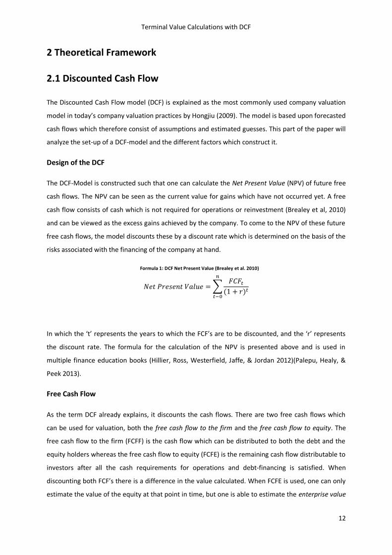
Formula 1: DCF Net Present Value (Brealey et al. 2010)
𝑁𝑒𝑡 𝑃𝑟𝑒𝑠𝑒𝑛𝑡 𝑉𝑎𝑙𝑢𝑒 = ∑𝐹𝐶𝐹𝑡
(1 + 𝑟)𝑡
𝑛
𝑡−0
In which the ‘t’ represents the years to which the FCF’s are to be discounted, and the ‘r’ represents
the discount rate. The formula for the calculation of the NPV is presented above and is used in
multiple finance education books (Hillier, Ross, Westerfield, Jaffe, & Jordan 2012)(Palepu, Healy, &
Peek 2013).
Free Cash Flow
As the term DCF already explains, it discounts the cash flows. There are two free cash flows which
can be used for valuation, both the free cash flow to the firm and the free cash flow to equity. The
free cash flow to the firm (FCFF) is the cash flow which can be distributed to both the debt and the
equity holders whereas the free cash flow to equity (FCFE) is the remaining cash flow distributable to
investors after all the cash requirements for operations and debt-financing is satisfied. When
discounting both FCF’s there is a difference in the value calculated. When FCFE is used, one can only
estimate the value of the equity at that point in time, but one is able to estimate the enterprise value
Terminal Value Calculations with DCF
13
when using the FCFF because with this you derive at the total value in excess of operations. The
latter is therefore the most used in valuating practices and is therefore also the predominant FCF
used in this paper. The FCFF can be assorted in the following order:
Earnings Before Interest and Taxes (EBIT) – Taxes = Net Operating Profit After Tax (NOPAT)
NOPAT + Depreciation and Amortization (D&A) – Capital Expenditures (CapEx) – Increase in net
working capital (NWC) = Free Cash Flow to Firm (FCFF)
The taxes are subtracted from the company’s EBIT firstly, providing an operation profit without
requirements outside of the company’s debt holders or investors. Secondly, the accounting amount
written in depreciation and amortization is added to the profit, this is done because the accounting
tool of depreciating assets or amortizing resources does not reflect an actual cash outflow for that
year. Thirdly, the capital expenditures in that year are subtracted from the NOPAT. Similar to the
D&A previously, although the capital expenditures most likely represent assets which will be used
for, and written off in, several years, these expenditures do reflect an actual cash outflow in this year
and should therefore be subtracted from the NOPAT. Lastly, the increase in net working capital
(NWC) should be subtracted. The NWC consists of the current assets minus the current liabilities, and
the requirement of a higher NWC reflects a cash outflow and should therefore be subtracted. The
resulting number reflects the free cash flow to the firm which can be used for DCF-valuation.
Discount Rate
When the future cash flows are estimated, they have to be given their current (present) value. This
can be done by discounting it using the appropriate discount rate. The appropriate rate is the rate
which the investors demand that the value would increase given the risks involved in that
investment.
Because companies usually have two types of financing in their capital structure, both the cost of the
equity raised, as the cost of the debt taken should be incorporated in the discount rate (Brealey et al.
2010). The ‘weight’ that both financing options should be given in the calculation depends on the
relative magnitude of them, resulting in a weighted average cost of capital, or WACC.
Cost of Debt
Debt is a financing option on which interest has to be paid by the borrower. There are different types
of debt which, depending on their duration and source, face different interest payments (costs). A
loan with a short duration and with a priority over different loans (senior debt) faces little risk for the
lender and it will therefore require a low interest rate, however, long-term debt may face an interest
Terminal Value Calculations with DCF
14
rate which is significantly higher due to the higher risk. Next to that, the situation of the borrower is a
highly influencing factor concerning the cost for debt. If a company is reckoned to be a stable and
reliable borrower, the financing source will, again focusing on its’ risk, demand a fairly low interest
rate, whereas an unstable and volatile company may face high costs regarding their loan. Because
the cost of debt can be subtracted from the taxable income, one should use the after-tax cost of debt
as the debt-input for the WACC resulting in the following cost of debt:
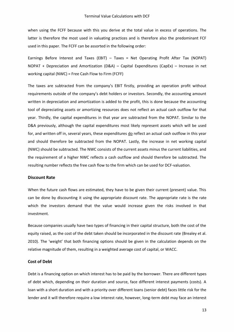
Formula 2: Cost of Debt (Palepu et al. 2013)
𝐶𝑜𝑠𝑡 𝑜𝑓 𝐷𝑒𝑏𝑡 = 𝑟𝑑 ∗ (1 − 𝑡)
In which the 𝑟𝑑 is the pre-tax cost of debt, and the 𝑡 is the tax rate.
Cost of Equity
The cost of equity can be derived using different models, a frequently used model is the Capital Asset
Pricing Model, or CAPM introduced by Sharpe in 1964. The three factors used in this model are the
risk-free rate, the market risk premium and the β (Beta). The risk-free rate, is the rate which every
investor/lender will get when they invest in the least fallible asset on the market. Damodaran (2008)
for example argues the 3 or 6 months T-bills which are backed by the U.S. government as a risk free
rate because these are almost non-fallible. The market risk premium are the combined risks to which
the asset at hand is exposed and which increase the fallibility of this investment. The systematic risk
or β (Beta) reflects the sensitivity of the cash flows to economy-wide market movements (Palepu et
al. 2013). The β represents the shift of the economy, and therefore the β of the economy is by
definition equal to 1. Companies which are highly sensitive to changes in the economy, such as
construction firms or luxury goods will have a β which is larger than 1 whereas less cyclical
companies will have a β below 1. These less sensitive stocks will lose less when the industry performs
badly, and will gain less when the industry is prosperous. The formula for the CAP-Model can be
written as is shown below.
Formula 3: Cost of Equity (Sharpe. 1964)
𝐶𝑜𝑠𝑡 𝑜𝑓 𝐸𝑞𝑢𝑖𝑡𝑦 = 𝑟𝑓 + 𝛽(𝑟𝑚 − 𝑟𝑓)
Both the cost of debt, as the cost of equity will be incorporated in the weighted average cost of
capital (WACC) in which the combined cost of financing can be calculated.
Terminal Value Calculations with DCF
15
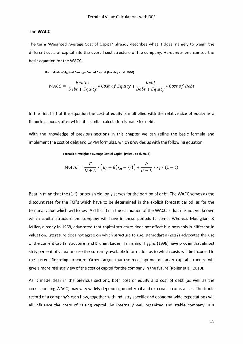
The WACC
The term ‘Weighted Average Cost of Capital’ already describes what it does, namely to weigh the
different costs of capital into the overall cost structure of the company. Hereunder one can see the
basic equation for the WACC.
Formula 4: Weighted Average Cost of Capital (Brealey et al. 2010)
𝑊𝐴𝐶𝐶 = 𝐸𝑞𝑢𝑖𝑡𝑦
𝐷𝑒𝑏𝑡 + 𝐸𝑞𝑢𝑖𝑡𝑦∗ 𝐶𝑜𝑠𝑡 𝑜𝑓 𝐸𝑞𝑢𝑖𝑡𝑦 +
𝐷𝑒𝑏𝑡
𝐷𝑒𝑏𝑡 + 𝐸𝑞𝑢𝑖𝑡𝑦∗ 𝐶𝑜𝑠𝑡 𝑜𝑓 𝐷𝑒𝑏𝑡
In the first half of the equation the cost of equity is multiplied with the relative size of equity as a
financing source, after which the similar calculation is made for debt.
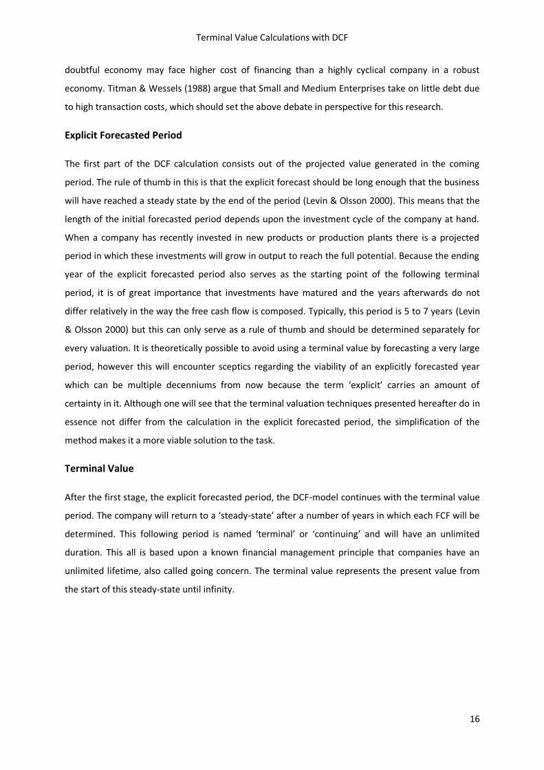
With the knowledge of previous sections in this chapter we can refine the basic formula and
implement the cost of debt and CAPM formulas, which provides us with the following equation
Formula 5: Weighted average Cost of Capital (Palepu et al. 2013)
𝑊𝐴𝐶𝐶 = 𝐸
𝐷 + 𝐸∗ (𝑅𝑓 + 𝛽(𝑟𝑚 − 𝑟𝑓)) +
𝐷
𝐷 + 𝐸∗ 𝑟𝑑 ∗ (1 − 𝑡)
Bear in mind that the (1-𝑡), or tax-shield, only serves for the portion of debt. The WACC serves as the
discount rate for the FCF’s which have to be determined in the explicit forecast period, as for the
terminal value which will follow. A difficulty in the estimation of the WACC is that it is not yet known
which capital structure the company will have in these periods to come. Whereas Modigliani &
Miller, already in 1958, advocated that capital structure does not affect business this is different in
valuation. Literature does not agree on which structure to use. Damodaran (2012) advocates the use
of the current capital structure and Bruner, Eades, Harris and Higgins (1998) have proven that almost
sixty percent of valuators use the currently available information as to which costs will be incurred in
the current financing structure. Others argue that the most optimal or target capital structure will
give a more realistic view of the cost of capital for the company in the future (Koller et al. 2010).
As is made clear in the previous sections, both cost of equity and cost of debt (as well as the
corresponding WACC) may vary widely depending on internal and external circumstances. The track-
record of a company’s cash flow, together with industry specific and economy-wide expectations will
all influence the costs of raising capital. An internally well organized and stable company in a
Terminal Value Calculations with DCF
16
doubtful economy may face higher cost of financing than a highly cyclical company in a robust
economy. Titman & Wessels (1988) argue that Small and Medium Enterprises take on little debt due
to high transaction costs, which should set the above debate in perspective for this research.
Explicit Forecasted Period
The first part of the DCF calculation consists out of the projected value generated in the coming
period. The rule of thumb in this is that the explicit forecast should be long enough that the business
will have reached a steady state by the end of the period (Levin & Olsson 2000). This means that the
length of the initial forecasted period depends upon the investment cycle of the company at hand.
When a company has recently invested in new products or production plants there is a projected
period in which these investments will grow in output to reach the full potential. Because the ending
year of the explicit forecasted period also serves as the starting point of the following terminal
period, it is of great importance that investments have matured and the years afterwards do not
differ relatively in the way the free cash flow is composed. Typically, this period is 5 to 7 years (Levin
& Olsson 2000) but this can only serve as a rule of thumb and should be determined separately for
every valuation. It is theoretically possible to avoid using a terminal value by forecasting a very large
period, however this will encounter sceptics regarding the viability of an explicitly forecasted year
which can be multiple decenniums from now because the term ‘explicit’ carries an amount of
certainty in it. Although one will see that the terminal valuation techniques presented hereafter do in
essence not differ from the calculation in the explicit forecasted period, the simplification of the
method makes it a more viable solution to the task.
Terminal Value
After the first stage, the explicit forecasted period, the DCF-model continues with the terminal value
period. The company will return to a ‘steady-state’ after a number of years in which each FCF will be
determined. This following period is named ‘terminal’ or ‘continuing’ and will have an unlimited
duration. This all is based upon a known financial management principle that companies have an
unlimited lifetime, also called going concern. The terminal value represents the present value from
the start of this steady-state until infinity.
Terminal Value Calculations with DCF
17
2.2 Terminal Value Calculations
The different terminal value calculations are hereunder presented and explained in which the
differences are made clear. One should take into account that different terminal value calculations
do not by definition result in different valuation outcomes. The techniques are selected based upon
the progression made upon the same DCF-idea and the applicability for practitioners. Reis & Augusto
(2013) show that there are differences in complexity and the different models are presented in an
ascending order of complexity.
Intrinsic value
A basic valuation method is the method in which the intrinsic value of the company is calculated. The
value is composed out of the combined sale of all the assets minus the liabilities the company is
required to repay to its creditors. If a company is expected to have no added value after the explicit
forecasted period, one can use this intrinsic value as a terminal value calculation. Companies for
which such a method could be suitable are for example those that serve in an industry which could
become obsolete after a certain period due to technological innovation. Also companies which are
built to serve for a particular project or a particular period in time might be valued in such a way.
Costs of replacement as a terminal value
In the book “Valuation: Measuring and Managing the value of Companies” the concept of
replacement costs as a way to calculate the terminal value has been explained by Koller et al. (2010).
The theory is based around the idea that the terminal value is equal to the expected costs to replace
the assets of the company. Drawbacks to this theory are that not all tangible and certainly not all
intangible assets are replaceable. Next to that, some assets within a company might still add value to
a company but will not be replaced in case of malfunction due to the limited added value. This would
therefore result in an overestimation of the value of the company. Although both the intrinsic value
technique as the cost of replacement are not seen as a traditional terminal value calculation for DCF,
these are incorporated in this thesis due to the applicability of these techniques in practice. The
fundamental differences in assumptions to the techniques that follow can serve as an example for
the different choices made by practitioners.
Terminal Value Calculations with DCF
18
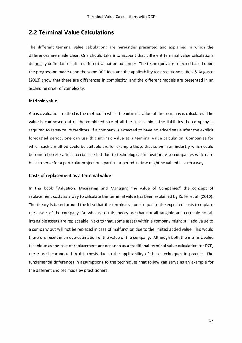
Basic Perpetuity
A perpetuity is a common model in DCF valuation techniques, the most simple version of which can
be stated as follows.
Formula 6: Terminal Value Basic Perpetuity
𝑇𝑉 =𝑁𝑂𝑃𝐴𝑇𝑡+1
𝑊𝐴𝐶𝐶
In this the net operating profit after taxes will be divided by the weighted average cost of capital. The
perpetuity is a mathematical trick to calculate the outcome of an infinite series, in this case the
present value of the net profits of all the years to come. In this method there is no acknowledgement
of potential growth so even if the company sees investment opportunities, the return will be equal to
the cost of capital. Over a longer period of time companies usually revert to a state of no real growth
which therefore makes the assumption reasonable for some industries and mature companies.
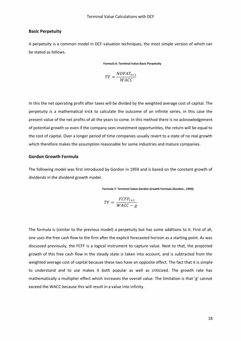
Gordon Growth Formula
The following model was first introduced by Gordon in 1959 and is based on the constant growth of
dividends in the dividend growth model.
Formula 7: Terminal Value Gordon Growth Formula (Gordon., 1959)
𝑇𝑉 = 𝐹𝐶𝐹𝐹𝑡+1
𝑊𝐴𝐶𝐶 − 𝑔
The formula is (similar to the previous model) a perpetuity but has some additions to it. First of all,
one uses the free cash flow to the firm after the explicit forecasted horizon as a starting point. As was
discussed previously, the FCFF is a logical instrument to capture value. Next to that, the projected
growth of this free cash flow in the steady state is taken into account, and is subtracted from the
weighted average cost of capital because these two have an opposite effect. The fact that it is simple
to understand and to use makes it both popular as well as criticized. The growth rate has
mathematically a multiplier effect which increases the overall value. The limitation is that ‘g’ cannot
exceed the WACC because this will result in a value into infinity.
Terminal Value Calculations with DCF
19
Koller Value Driver Formula
A more detailed approach of the Gordon growth model can be given with the value driver formula of
Koller et al (2010).
Formula 8: Terminal Value Koller Value Driver Formula (Koller et al. 2010)
𝑇𝑉 = 𝑁𝑂𝑃𝐿𝐴𝑇𝑡+1 (1 −
𝑔𝑅𝑂𝑁𝐼𝐶
)
𝑊𝐴𝐶𝐶 − 𝑔
In this, the term RONIC needs to be explained, as being the expected rate of return on newly
invested capital, which is capital which has not been put in place yet. Although the formula looks
more complex, this will result in the same valuation outcome, given that the input parameters are
consistent. Where the free cash flow to the firm is the numerator in the Gordon growth model, the
numerator in this formula actually represents the same input when the reasoning behind the
approach is the same.
The advantage in this model, compared with the Gordon growth model is the use of the RONIC which
defines the relationship between the terminal growth and the investment to be put in place to reach
this growth. A predefined expected return on newly invested capital means that an increase in
growth as an outlook for the firm would therefore require a higher percentage of the operating profit
to be invested (or retention rate) and this would therefore lower the free cash flow.
Koller two-stage Value Driver Formula
In addition to the value driver formula, the two-staged formula has been introduced by Koller et al
(2010). In this the expected return on newly invested capital ‘RONIC’ has been introduced in 2 stages
A and B, this correlates with the different growth rates in both stages.
Formula 9: Terminal Value Koller Two-stage Value Driver Formula (Koller et al. 2010)
𝑇𝑉 = (𝑁𝑂𝑃𝐿𝐴𝑇𝑡+1 (1−
𝑔𝑎𝑅𝑂𝑁𝐼𝐶𝑎
)
𝑊𝐴𝐶𝐶− 𝑔𝑎)(1 − (
1+ 𝑔𝑎
1+𝑊𝐴𝐶𝐶)𝑁) + (
𝑁𝑂𝑃𝐿𝐴𝑇𝑡+1(1+𝑔𝑎)𝑁(1−𝑔𝑏
𝑅𝑂𝑁𝐼𝐶𝑏)
(𝑊𝐴𝐶𝐶−𝑔𝑏)(1+𝑊𝐴𝐶𝐶)𝑁 )
In this the 𝑔𝑎 is the growth-rate in the initial period of the terminal value and is 𝑔𝑏 the growth-rate
in the stable period. The usefulness of this more complex calculation is more apparent in valuations
Terminal Value Calculations with DCF
20
for high-growth companies or companies which are expected to yield abnormal returns after the
explicit forecasted period. The reasoning behind the usage of two stages lies in the fact that valuators
have the possibility for a transitional period between the explicit forecasted period and the terminal
period. Growth rates do therefore not need to make an unrealistic drop after the first part of the
valuation.
The Three-stage Terminal Value model
The final model presented was introduced by Fuller and Hsia (1984) and served as a Dividend
Discount Model with multiple stages. Damodaran (2012) implemented this as a terminal Value
technique for a DCF-model in which the terminal value calculation is also subdivided in multiple
stages. The previous two-stage TV model assumes a different (lower) growth rate after the first
stage. This model assumes the same but with the addition that the growth rate in the first stage
gradually declines towards the latter (more definite) stable growth rate. The rationale behind this is
that growth does not increase or decline in drastic steps, but that it follows a trend before it
stabilizes on a new rate.
Formula 10: Terminal Value The Three-stage TV model (Damodaran 2012)
𝑇𝑉 = 𝐹𝐶𝐹𝐹0 ∗ (1 + 𝑔)𝑡
(1 + 𝑟)𝑡+ ∑
𝐹𝐶𝐹𝐹𝑡
(1 + 𝑟)𝑡+
𝐹𝐶𝐹𝐹𝑛+1
(𝑟 − 𝑔𝑛) ∗ (1 + 𝑟)𝑛
𝑡=𝑛2
𝑡=𝑛1+1
The 3 different parts of the equation represent the initial high growth part, the transition part and
the stable growth-rate part of the terminal value calculation.
Terminal Value Calculations with DCF
21
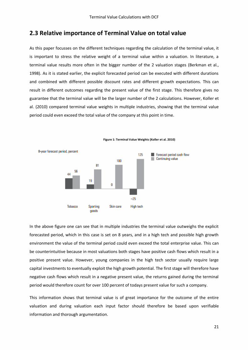
2.3 Relative importance of Terminal Value on total value
As this paper focusses on the different techniques regarding the calculation of the terminal value, it
is important to stress the relative weight of a terminal value within a valuation. In literature, a
terminal value results more often in the bigger number of the 2 valuation stages (Berkman et al.,
1998). As it is stated earlier, the explicit forecasted period can be executed with different durations
and combined with different possible discount rates and different growth expectations. This can
result in different outcomes regarding the present value of the first stage. This therefore gives no
guarantee that the terminal value will be the larger number of the 2 calculations. However, Koller et
al. (2010) compared terminal value weights in multiple industries, showing that the terminal value
period could even exceed the total value of the company at this point in time.
Figure 1: Terminal Value Weights (Koller et al. 2010)
In the above figure one can see that in multiple industries the terminal value outweighs the explicit
forecasted period, which in this case is set on 8 years, and in a high tech and possible high growth
environment the value of the terminal period could even exceed the total enterprise value. This can
be counterintuitive because in most valuations both stages have positive cash flows which result in a
positive present value. However, young companies in the high tech sector usually require large
capital investments to eventually exploit the high growth potential. The first stage will therefore have
negative cash flows which result in a negative present value, the returns gained during the terminal
period would therefore count for over 100 percent of todays present value for such a company.
This information shows that terminal value is of great importance for the outcome of the entire
valuation and during valuation each input factor should therefore be based upon verifiable
information and thorough argumentation.
Terminal Value Calculations with DCF
22
2.4 Growth Patterns in DCF Terminal Value Calculations
As can be seen in the previous sections, there are multiple terminal value calculation techniques
developed in the past decades. The aim of every technique is to valuate a company in a way that is
the most comprehensive. Within the calculation of terminal value, the input parameter of growth of
great importance, and Martins (2011) explains that any changes, no matter how insignificant, could
have a significant influence on the value of the company. As explained in section 2.2 the increase of
complexity in the valuation model also translates in 3 different growth patterns.
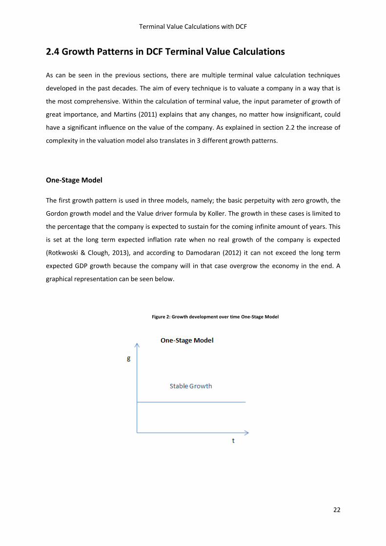
One-Stage Model
The first growth pattern is used in three models, namely; the basic perpetuity with zero growth, the
Gordon growth model and the Value driver formula by Koller. The growth in these cases is limited to
the percentage that the company is expected to sustain for the coming infinite amount of years. This
is set at the long term expected inflation rate when no real growth of the company is expected
(Rotkwoski & Clough, 2013), and according to Damodaran (2012) it can not exceed the long term
expected GDP growth because the company will in that case overgrow the economy in the end. A
graphical representation can be seen below.
Figure 2: Growth development over time One-Stage Model
Terminal Value Calculations with DCF
23
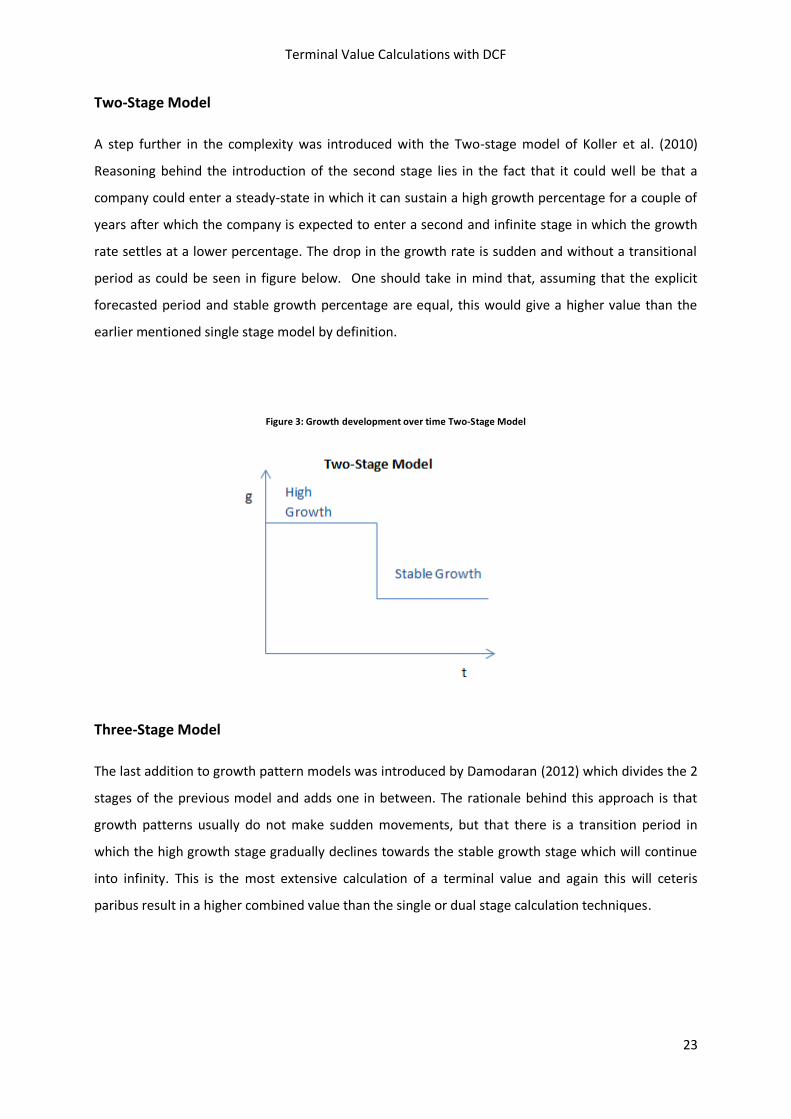
Two-Stage Model
A step further in the complexity was introduced with the Two-stage model of Koller et al. (2010)
Reasoning behind the introduction of the second stage lies in the fact that it could well be that a
company could enter a steady-state in which it can sustain a high growth percentage for a couple of
years after which the company is expected to enter a second and infinite stage in which the growth
rate settles at a lower percentage. The drop in the growth rate is sudden and without a transitional
period as could be seen in figure below. One should take in mind that, assuming that the explicit
forecasted period and stable growth percentage are equal, this would give a higher value than the
earlier mentioned single stage model by definition.
Figure 3: Growth development over time Two-Stage Model
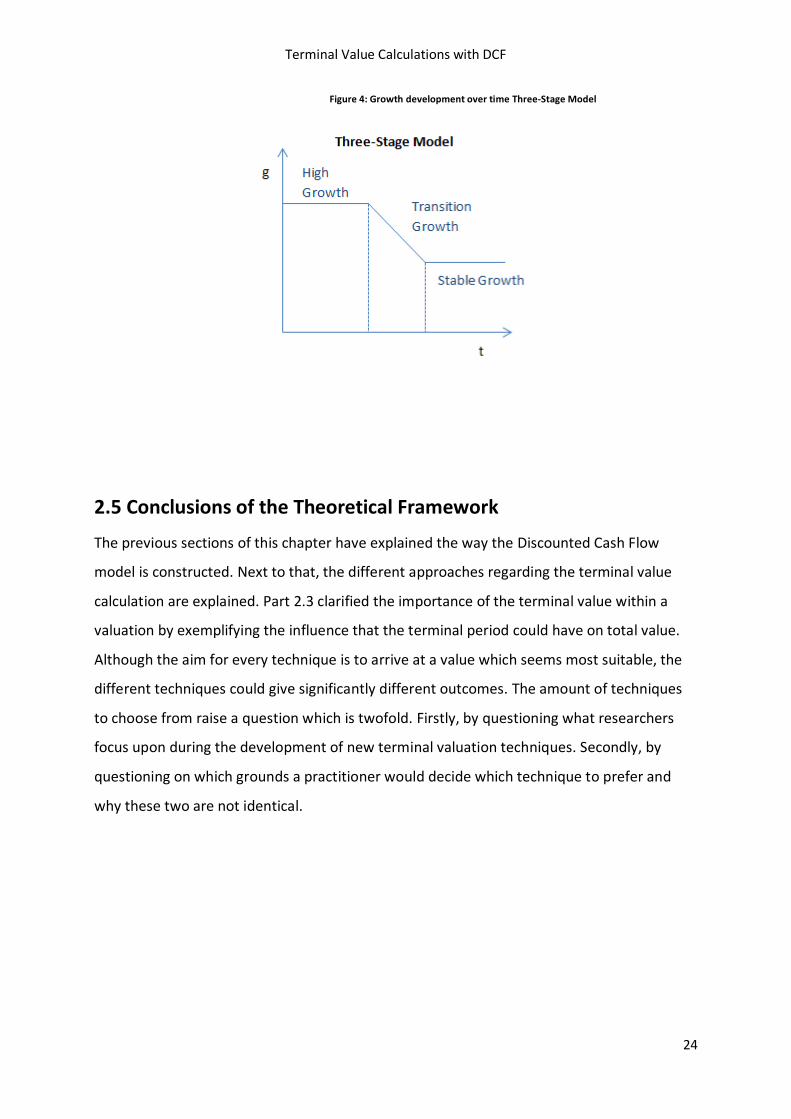
Three-Stage Model
The last addition to growth pattern models was introduced by Damodaran (2012) which divides the 2
stages of the previous model and adds one in between. The rationale behind this approach is that
growth patterns usually do not make sudden movements, but that there is a transition period in
which the high growth stage gradually declines towards the stable growth stage which will continue
into infinity. This is the most extensive calculation of a terminal value and again this will ceteris
paribus result in a higher combined value than the single or dual stage calculation techniques.
Terminal Value Calculations with DCF
24
Figure 4: Growth development over time Three-Stage Model
2.5 Conclusions of the Theoretical Framework
The previous sections of this chapter have explained the way the Discounted Cash Flow
model is constructed. Next to that, the different approaches regarding the terminal value
calculation are explained. Part 2.3 clarified the importance of the terminal value within a
valuation by exemplifying the influence that the terminal period could have on total value.
Although the aim for every technique is to arrive at a value which seems most suitable, the
different techniques could give significantly different outcomes. The amount of techniques
to choose from raise a question which is twofold. Firstly, by questioning what researchers
focus upon during the development of new terminal valuation techniques. Secondly, by
questioning on which grounds a practitioner would decide which technique to prefer and
why these two are not identical.
Terminal Value Calculations with DCF
25
3 Methodology
3.1 Introduction
After the clarification of the theory in valuation as a whole and with a more focused look upon the
different techniques regarding the calculation of the terminal value, this section explains how the
methodology of this research is constructed. The research design will explain in which manner the
goal of the paper is achieved. After the explanation of the aimed target the methodology
subsequently will continue with the way the data is collected, and the manner in which the data will
be analyzed to come up with the conclusions.
3.2 The Research design
In this section the research design will be introduced. In this, the units of observation , the time scale
and the type of analysis are explained. Each design has limitations regarding the reliability of the way
it is conducted, and eventually also on the results fort flowing from the research, these will be
touched upon in the last part of this section. The goal of this paper is to explain the differences
between how practice conducts terminal value calculations, and how theory argues it should be.
According to Babbie (2004) this can be viewed as an explanatory research.
When looking at the time horizon (or dimension) the study will have a cross sectional design because
the observations that are to be made are all on the same point in time and place Babbie (2004).
Gerring, (2012) which views this cross sectional studies as ‘non randomized’ makes the distinction
between large samples which suggest a quantitative study and small samples which suggest a
qualitative study. The amount of observations are low and a qualitative design will be opted to
explain why the differences occur, and how big the differences are. The valuation reports, together
with the interviews which clarify them will be the units of observation and the units of analysis will
be the differences at hand. The aim is to investigate the valuation reports and it is expected that
these differ from theory. The input factors which account for these differences have to be analyzed.
The collection of the data is quite straightforward in this research because valuators have made their
reports available. The sample which is used is chosen by both the researcher as the professional
valuators to make sure that interesting reports are picked, and differences could be easily spotted
which serves the validity of the research. Because the reports are hand-picked this could therefore
be described as purposive sampling (Babbie, 2004). The amount of reports and the corresponding
Terminal Value Calculations with DCF
26
interviews (units of observation) used in order to get a representative sample 12, at which Guest et
al. (2006) explain that data saturation is achieved, but in this case a sample of 6 will already give a
good insight in the differences. All the chosen reports will consist of a valuation for a small or
medium enterprise. Because the sample was purposely chosen, it is impossible to make a
generalizable conclusion. The lack of a generalizable conclusion decreases the validity of the research
(Gerring, 2012). The lack of quantitative data perhaps lowers the reliability of the results but the use
of qualitative data serves as a possibility to find differences which might not have been thought of
before. The validity can be viewed as ‘high’ for internal purposes, but outside the scope of the
research the validity is low and it can at most be used as a starting point for other organizations to
also conduct such a research.
3.3 Collection and Analysis
The collection of the data which serves as a base for the research is twofold. There is research in
both literature as there is in practice. The first is an analysis based around the papers and books
which aimed at constructing the best DCF terminal value technique. Literature was analyzed by
distilling the reasoning behind the adjustments and differences to the existing terminal value
techniques. The main target in this is to describe why researchers try to improve the models and why
they think this is a valuable addition. The sections in which authors argue why their model prevails
over previous models are most interesting in this case. These quotes are selected and categorized.
An overview will be constructed in which the main focus points are listed. This part of the research
aims at answering sub-question 1 of the research question.
The second part of the research is focusing on the criteria which compose the choice for the terminal
value calculation in practice. The collection of data from which to draw conclusions has two sides to
it. Firstly by examining actual valuation reports which describe the chosen method and support this
with argumentation. Secondly by having semi-structured interviews with the practitioners which
constructed the previously mentioned valuation reports. The interviews are semi-structured to give
the researcher the opportunity to extract information which goes beyond the scope of the interview
by asking new questions which arise during the conversations. The initial interview questions are
developed by connecting the theory to practical difficulties and differences. To gain a more coherent
insight in the reasoning of the practitioner, the questions are not limited to the scope of the terminal
value period alone.
Terminal Value Calculations with DCF
27
Interview Questions
The following questions are constructed to gain an insight in the practitioners calculations of the
terminal value with the DCF model.
Forecasted period
1: a) Although literature states that it does not affect the value as a whole, what is usual duration of
the explicit forecasted period in your calculations? Do you take the investment-cycle and the so
called steady-state into account?
b) When do you deviate from that choice?
WACC
2: a) To what extend is the used WACC in this explicit forecasted period applicable to use for the
calculation of the terminal value?
b) How do you see the option of an ‘optimal structure’ when there is space for improvement
regarding the capital structure?
Terminal value:
Technique:
3: a)Which technique do you use whilst calculating a terminal value?
b) Do you deviate from this model, if so, when?
4: What focus points serve as a base for this choice?
5: How do you estimate the expected growth for this stage, and in which bandwidth are these
percentages usually?
6: To what extend does this deviate on average from the growth-rate used in the explicit forecasted
period?
7: Most authors advocate that companies can not outperform the entire economy in the terminal
period. This is due to the fact that mathematically the company will eventually outgrow the
economy. How do you rate this argument?
8: Between 84 and 94 percent of the terminal value is accumulated in the first 20 years of the
terminal period (using a Gordon Growth model with growth between 0 and 5 percent)(Rotkowski &
Clough, 2013). Could you imagine that companies are able to outperform an economy for this
period? (How does this affect the previous question/answer?)
9: How do you see an extra stage between the explicit forecasted period and terminal period to
gradually decrease the growth to the stable rate?
10: How do you rate the value of the terminal period in relation with the value during the explicit
forecasted period, and is this too high? (This can exceed 100% for high growth companies)
Terminal Value Calculations with DCF
28
11: Do you think that the unpredictable nature of a terminal value calculation causes you to use
somewhat more conservative input for the calculation?
In General
The following questions could to a certain extend overlap with previous questions but serve to even
better understand the train of thoughts behind the chosen techniques.
12: Do you feel that you as a practitioner mainly calculate a ‘value’ or a ‘price’ when you supervise a
takeover?
13: Does the situation of the seller/buyer sometimes influences the calculation?
14: Do you think that the construction of a ‘possible value’ (perhaps whilst using a better than actual
capital structure) is an addition to the valuation report? Are there more options than the use of a
more optimal WACC?
15: In general, how big a portion of the total value could in your eyes be attributable to the seller
during a takeover? Does this also represent the difference between ‘value’ and ‘price’? And to what
extend is the size of the company a factor in this?
Analysis
The extracted information is rephrased and summarized by the researcher during the interviews to
check the validity and decrease the possibility of false interpretations. The semi-structured nature of
the interview provides this research with a good representation of the so called ‘gut-feeling’ of
practitioners when it comes to valuation. This qualitative approach is in this case more valuable due
to the soft-skill nature of valuations. The aim of the research in valuation reports and interviews is to
answer sub-question 2 of the research question and partially gain an insight for sub-question 3. The
Dutch version of the interview can be found in Appendix III.
Terminal Value Calculations with DCF
29
4 Results
4.1 Introduction
The previous chapter has focused upon the way the research could be structured and how data could
be collected. This chapter will focus on the outcome of this research. For both literature and practice
this research will narrow the amount of factors down to the four most dominant. The four most
relevant and frequent issues mentioned by authors are selected and these represent the focus points
for literature. The four criteria which were most distinguished and present in valuation reports and
interviews will be used for the analysis in practice. At the end of the coming sections, the focus
points and criteria will be graded against each other for which a five point scale will serve as a
grading measurement. The scores can vary from ‘++’ to ‘--‘ and ‘±’ is the middle grade.
4.2 Focus in Literature on Terminal Value Calculations
Within terminal value calculations, literature strives for a model in which uncertainty is as low as
possible and in which the resulting value can be argued the strongest. For this, the quality of the key
input factors determine the quality of the technique. Although multiple techniques could deliver the
same value when the same assumptions serve as a basis for the calculation, the strength of the
arguments resulting in these assumptions differ between them.
A separation can be made between internal and external (and a mixed) input for the valuation. A
focus point which gives a better view of the company’s side of the valuation is an internal analysis
focus point. An external focus point is a point which is determined by factors surrounding the
company, such as the state of the industry and economy. The third category is a mixed focus point
where both company and external factors determine the outcome. This section aims to create an
overview of these key focus points for the improvement of terminal value calculations and looks to
distinguish the differences between them. A table will summarize the findings in the concluding
stage of this section.
Terminal Value Calculations with DCF
30
Consistency
The first factor described in literature as to improve the terminal value techniques is consistency. As
consistency is a very broad and widely used term in most research, the term is not used as a fashion
term in this thesis. Although the intrinsic value and replacement cost techniques are consistent with
the accumulated value of the individual items, there is usually no consistency between these values
and the expected value forth flowing from operations of a company. Multiple authors have aimed to
approach this problem. Whereas the basic perpetuity already incorporates the going concern
principle in the fact that the terminal value calculation is a perpetuity, the Gordon growth model
takes this a step further. Gordon (1959) makes use of a stable growth rate after the explicit
forecasted period to valuate according to expectations even in the distant future. This already is a
new step in consistency because from growth in the initial period to zero growth hereafter without
explanation or valid argumentation decreases the validity of the valuation. Koller et al. (2010) takes
consistency a step further in both its single and two-stage model. This is due to the introduction of
the return on newly invested capital (RONIC) and the relationship with the terminal growth rate.
Koller argues that although under the same assumptions the value driver formula is equivalent to the
Gordon growth model, but the latter increases the chance of a conceptual error by not taking into
account the level of free cash flow which is consistent with the growth rate. The three stage model
by Damodaran (2012) improves consistency by adding a natural pattern in growth rates. The
transitional stage creates an opportunity to better argument the expected growth pattern. These
statements implicate that a terminal value calculation should be consistent in assumptions made and
should respect the interdependent relationships between numbers. A growth rate should be in
accordance with forecasted investments, their returns and WACC.
Transparency
The second factor that literature tries to constantly improve with new models is the level of
transparency. Similarly to the term ‘consistency’ the term transparency may seem somewhat
obvious. However, there are some differences in transparency regarding different terminal value
techniques.
Koller et al. (2010) proved with the value driver formula that the relationship between growth and
investment needed for that growth could be seen prominently in the terminal value calculation. The
addition of this reduces space for questions regarding assumed growth rates. The introduction of the
third stage by Damodaran (2012) increases transparency between the growth rates chosen.
Terminal Value Calculations with DCF
31
From this it can be concluded that a terminal value should be transparent in the sense that the result
is a logical outcome from the logically argued input factors. The transparency is increased when the
terminal value leaves little space for questions. An increase in the amount of input parameters
forces the valuator to strengthen its argumentation and results in a higher transparency. The
increase in complexity and amount of input factors also increases the amount of argumentation with
which a valuator supports the assumptions. This puts the value driver formula and the two- and
three-stage models in a better position regarding the level of compliance with this focus point.
Sensible Growth
A third element in which authors try to improve their models can be summarized as sensible growth.
Whereas the basic perpetuity does not even take growth into account, Gordon (1959) already
explained that growth can be expected even beyond the explicit forecasted period. The addition of a
stable growth rate for the terminal period was introduced by him. After this idea settled, multiple
authors sought ways of improving this idea. Koller et al. (2010) argues that terminal growth rates
should follow a natural pattern and have to be argued in a logical manner, with which he adds that in
certain situations, you may want to break up the continuing value. This is executed in his two-stage
model, by introducing a first high-growth stage which is followed by a second stable-growth stage.
Arguably this results in a more logical situation for companies which have an expected growth
difference somewhere in the future. A model which requires more thought about future growth
rates increases the validity and trustworthiness of the terminal value. Damodaran (2012) argues that
the implementation of a transition period follows an even more natural pattern. In this the two-stage
model is extended towards a three-stage model with a gradual decline in growth rate from high to
stable. Obviously, both intrinsic value and replacement costs as a way of computing the terminal
value do not take growth into account, therefore both score a minimum in this literature standard.
The basic perpetuity also does not take growth into account for the terminal period, but because in
some cases zero growth could be advocated as the best growth rate this is slightly less failing. From
the Gordon growth model onwards, the increase in complexity gives valuators a broader set of
opportunities at the starting point and therefore increasingly comply with the sensible growth rate
focus point.
Terminal Value Calculations with DCF
32
Extensive market analysis
A company moves within an industry and this industry moves in an economy, therefore there is a
relation between the state of the economy and the state of the company. Valuators should therefore
not only investigate the expectations of the company, but also the expectations of the economy as
whole. For instance the expected growth rate of the entire economy could influence the expected
growth rate for the company at hand. Shaked and Kempianen (2009) state that there is a close link
between growth rates in the terminal period and inflation of the economy. Damodaran (2006) adds
that a company can not sustain a higher growth than the expected growth of the economy in the
terminal period because mathematically the company should outgrow the size of the rest of the
economy. From these statements one can conclude that the optimal model should force a valuator
to also investigate the industry and economy. Whereas intrinsic value barely is influenced by the
market analysis, replacement costs are just slightly more applicable. One can argue that the state of
the economy influences prizes which affect the replacement costs. However, no extensive analysis is
required for these two techniques. The basic perpetuity could be used for a valuation during
stagnation of the economy but the Gordon growth model forces the valuator to take the state of the
economy into account because of the stable growth rate which has to be computed for the terminal
period and which partially is influenced by it. The two and three-staged models provide
opportunities for valuators to increase the level of detail regarding the influence of the economy on
the value, and therefore score higher points.
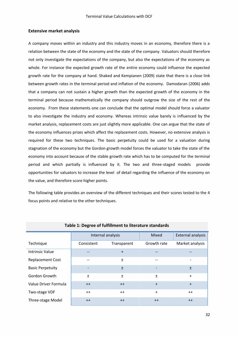
The following table provides an overview of the different techniques and their scores tested to the 4
focus points and relative to the other techniques.
Table 1: Degree of fulfillment to literature standards
Internal analysis Mixed External analysis
Technique Consistent Transparent Growth rate Market analysis
Intrinsic Value -- + -- --
Replacement Cost -- ± -- -
Basic Perpetuity - ± - ±
Gordon Growth ± ± ± +
Value Driver Formula ++ ++ + +
Two-stage VDF ++ ++ + ++
Three-stage Model ++ ++ ++ ++
Terminal Value Calculations with DCF
33
4.3 Focus of Practitioners on Terminal Value Calculations
Now that it is clear on which grounds literature tries to increase the validity and trustworthiness of
the terminal value calculation, this section reviews the motivations of valuators in practice to come
up with a terminal value for the customers they support. The following is based upon a review from
practice-case valuation reports and from supporting (semi-structured) interviews with those who
constructed these reports. The goal is to identify the reasons behind the choices of valuators with
respect to the technique they prefer. In this process it is possible to distinguish between different
categories of analysis. The category “Internal Analysis” represents the focus-points that practitioners
have regarding the valuation of the company at hand. In the category “External Analysis” the
practicality of the (to be determined) value is checked for other parties which are involved. The third
category “Mixed” represents the focus which lies on the intersection of both the company at hand,
and the counterpart. The goal of this section is to construct a table which tests the applicability of the
different terminal valuation techniques to the focus of practitioners.
Dependency
A major focus point that came forward in the valuation reports and the supporting interviews is the
dependency of the (to be valuated) company towards both its management and its customers. A
company which is conceived to be largely dependent to either one of them faces uncertainty which
has a depressing effect on price.
Respondent: “Companies which are very dependent of the manager or certain key figures within the
company could not be valued solely based on prospects created by this management”
A different practitioner added:
Respondent: “An entrepreneur who does not care for his successor destroys part of the value of the
firm”
A second dependency factor can be found in the spectrum of customers from the company. Are
customers solely based within one industry, and does a change in that industry therefore affect the
company directly. Does the firm has multiple small customers or does it rely on 1 or 2 large clients. A
valuator declared:
Respondent: “Dependency of one or few customers decreases the price of the company because the
risk of decreasing income is higher”
Terminal Value Calculations with DCF
34
This therefore clarifies that dependency on both the quality or network of its key figures, or
dependency of its clients will influence the price of the firm in a negative way. Whilst using the
intrinsic value or replacement cost technique, the dependency factor does not play a role. This is
totally due to the company as such. For a basic perpetuity or the Gordon growth model, the fact that
this is based on future cash flows makes that valuators already apply a more conservative approach.
The value driver formula, the two- and three-stage model imply a higher value for the distant future
which makes the practitioner more hesitant. These are therefore not seen as the best options.
Attribution
Within the process of valuation of small and medium enterprises, the valuators faces the question
which portion of the future cash flows and corresponding value could be attributed to the manager
shareholder(s) which sell or leave the company at this moment in time. Should the entire portion of
value forth flowing from (especially more distant) future cash flows be taken into account. Although
this again creates the gap between ‘value’ and ‘price’ a respondent described the situation as
follows:
Respondent: “During the takeover process a buyer sees future growth as a gain he or she can collect,
because this is up to them to achieve”
Whereas literature sees future growth as a logical outcome from the path set by the current owners,
SME entrepreneurs see this more as their own achievements. This therefore creates a practical
problem for valuators to use a growth factor in the terminal value period. This problem does not
occur for the first three terminal value techniques. But from the Gordon growth model onwards
there is a decrease in applicability for the more complex models due to the higher portions of value
corresponding with the growth.
Terminal Value Calculations with DCF
35
Deal making
A third decision criteria for practitioners is the amount of practicality when it comes down to making
a deal. Next to the valuation process, corporate finance companies also serve as dealmakers, and
even though valuation outcomes only serve as a starting point for negotiation according to Svetlova
(2012), the valuation outcome which discourages either the seller or the buyer in this process will
frustrate the creation of a deal. Both very low as very high valuation outcomes could therefore be
seen as undesirable. One of the respondents commented as follows:
Respondent: “During the process of a takeover we usually are at the middle of a rope which is pulled
from both sides.”
And even though this is the most classical issue in the gap between ‘value’ and ‘price’ practitioners
do have to take their position into account.
Respondent: “When several deals fail due to the gap in value in the valuation report and expected
prices by both parties, we have not done a good job”
But, as was touched upon, this has implications for both sides of the value spectrum. The use of the
intrinsic value and replacement cost as a terminal value could seem interesting for buyers and could
be seen as too little value for sellers, whereas the Koller et al. (2010) and Damodaran (2012)models
may lead to an insurmountable price for the buyers. Practitioners therefore tend to choose the
golden mean in the basic perpetuity or the Gordon growth model.
Ability to fund
Related to the previous “deal making” section, the valuators are involved in the entire process of for
instance take-overs or buy-outs. The process does most of the times not end with a deal between the
different actors and it is more the rule than the exception that the buying side of the deal needs
financing for this business. The perceived difficulties that practitioners would encounter in this stage
could have a price depressing effect on the valuation. A lower price would normally result in easier
fundability. During the interviews, some of the respondents made the following or similar
statements:
Respondent: “ When the agreed price is perceived as ‘too high’ by possible financiers, the deal could
(even in that stage) be put to a hold, and ultimately fail”
Terminal Value Calculations with DCF
36
When asked if this is only taken into account during the talks about the takeover, one of them
responded:
Respondent: “I do take rules of thumb regarding the ability to fund into account during the
construction of the valuation report”
The order in which the terminal value techniques are listed have increasingly high outcomes in value,
this therefore has a contrariwise effect on the ability to fund for external financiers.
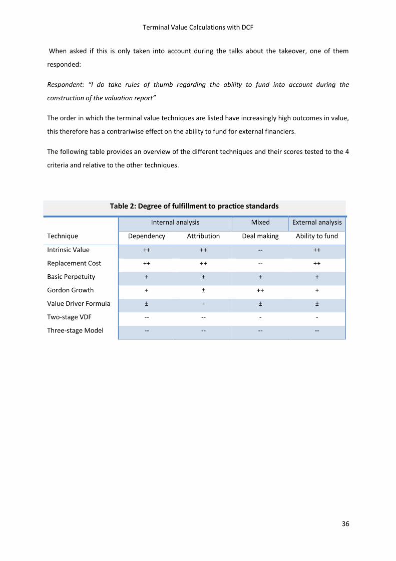
The following table provides an overview of the different techniques and their scores tested to the 4
criteria and relative to the other techniques.
Table 2: Degree of fulfillment to practice standards
Internal analysis Mixed External analysis
Technique Dependency Attribution Deal making Ability to fund
Intrinsic Value ++ ++ -- ++
Replacement Cost ++ ++ -- ++
Basic Perpetuity + + + +
Gordon Growth + ± ++ +
Value Driver Formula ± - ± ±
Two-stage VDF -- -- - -
Three-stage Model -- -- -- --
Terminal Value Calculations with DCF
37
4.4 How to approach differences between Literature and Practice
The tables in the previous sections show some striking differences in the points (plusses) that the
same techniques score in focus points for literature and in criteria for practice as in how to decide
the most suitable technique to use. In literature, authors try to improve the models on four pillars.
The four pillars of transparency, consistency, sensible growth rates and a better market analyses
score higher when models become more complex. These, more complex, models result in higher
output with similar input. On the other hand, there seems to be a certain reluctance for practitioners
to impose a terminal value calculation model which results in a high outcome. Although the input
factors most severely determine this outcome, these have to be supported by solid argumentation
and by choosing a different model these do not have to be altered. Whereas these conclusions seem
straightforward, the approach on how to bridge this gap is more difficult. The following results are a
combination of the ideas of the researcher and responses of practitioners. Valuators may want to
provide the various parties involved with more scenario based valuation calculations. One of the
respondents argued:
Respondent: “From our last 50 valuation reports, approximately 48 of them would contain the same
terminal value model. Only in cases of high exceptions we deviate from our dominant model ”
Because it is highly unlikely that 48 out of 50 valued companies were in the same position during the
valuation the predominant model used in practice might be chosen as the safe choice. To extend this,
valuators could also consider to incorporate sensitivity tables throughout the valuation report to
serve a dual purpose. First of all, a respondent claimed that an owner/director of a small or medium
enterprise is most likely not financially literate. And this hardens the process of explaining the
derived value.
Respondent: “A director (general owner) of a small company is more an entrepreneur than a financial
expert, the fact that he does not fully understand how the calculated value is build up makes it harder
to move him in a direction away from the targeted price he has in mind”
The sensitivity tables could possibly (partially) bridge this gap by clarifying how the different input
parameters influence the calculated value. Next to that, different values could at that point in time
be derived by explaining the different scenarios for the company and their respective consequences
for the input factors. This decreases the importance of the value derived in the valuation report and
gives the various parties involved a more ‘fluid’ starting point (Svetlova, 2012) in which
argumentation between the parties could influence the input parameters and, consequently, the
resulting value.
Terminal Value Calculations with DCF
38
5 Conclusions
This paper has gone through a couple of stages. The first stage aimed in creating an overall goal for
the thesis by stating a research question with sub-questions. After this, the theoretical framework
was constructed to put the theory in perspective and to be able to see the scope of the research.
This framework has showed several different DCF terminal value techniques. Most techniques are
based around the same line of thought but differ in terms of complexity. The theoretical framework
was concluded with the explanation of the importance of the terminal value in the overall value, and
the clarification around the different growth-rate patterns. The methodology sector explained that
this research has a qualitative design which has as goal to gain an insight on how literature and
practice differ in terminal value approaches. The latter was based around real life valuation reports
and semi-structured interviews. Both approaches were characterized by 4 pillars against which the
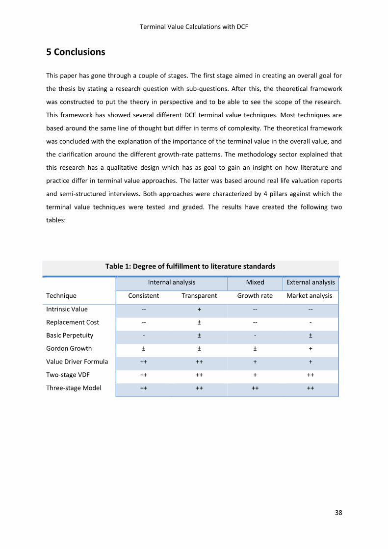
terminal value techniques were tested and graded. The results have created the following two
tables:
Table 1: Degree of fulfillment to literature standards
Internal analysis Mixed External analysis
Technique Consistent Transparent Growth rate Market analysis
Intrinsic Value -- + -- --
Replacement Cost -- ± -- -
Basic Perpetuity - ± - ±
Gordon Growth ± ± ± +
Value Driver Formula ++ ++ + +
Two-stage VDF ++ ++ + ++
Three-stage Model ++ ++ ++ ++
Terminal Value Calculations with DCF
39
Table 2: Degree of fulfillment to practice standards
Internal analysis Mixed External analysis
Technique Dependency Attribution Deal making Ability to fund
Intrinsic Value ++ ++ -- ++
Replacement Cost ++ ++ -- ++
Basic Perpetuity + + + +
Gordon Growth + ± ++ +
Value Driver Formula ± - ± ±
Two-stage VDF -- -- - -
Three-stage Model -- -- -- --
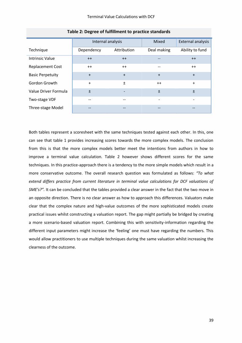
Both tables represent a scoresheet with the same techniques tested against each other. In this, one
can see that table 1 provides increasing scores towards the more complex models. The conclusion
from this is that the more complex models better meet the intentions from authors in how to
improve a terminal value calculation. Table 2 however shows different scores for the same
techniques. In this practice-approach there is a tendency to the more simple models which result in a
more conservative outcome. The overall research question was formulated as follows: “To what
extend differs practice from current literature in terminal value calculations for DCF valuations of
SME’s?”. It can be concluded that the tables provided a clear answer in the fact that the two move in
an opposite direction. There is no clear answer as how to approach this differences. Valuators make
clear that the complex nature and high-value outcomes of the more sophisticated models create
practical issues whilst constructing a valuation report. The gap might partially be bridged by creating
a more scenario-based valuation report. Combining this with sensitivity-information regarding the
different input parameters might increase the ‘feeling’ one must have regarding the numbers. This
would allow practitioners to use multiple techniques during the same valuation whilst increasing the
clearness of the outcome.
Terminal Value Calculations with DCF
40
6 Discussion, implications, limitations and future research
Discussion
The results give an insight in the logical development of literature, but also in the practical difficulties
the valuators have with these more complex models. The situation arises, that the value (whilst using
the more complex models) is in most cases very far of the price that may seem to be the ‘fair’ price.
This does, in my eyes, not take away the duty of the valuator to approach the ‘true value’ of the
company to the best of their abilities with the knowledge at hand. Having a conservative approach is
appropriate to a certain extent, but deliberately choosing models and input factors to come up with a
commercially more interesting value has some negatives to it which may harm not only the
trustworthiness of the valuator at hand, but also the reliability of the financial services as a whole. On
the other hand, the practical contradictions which are faced by the practitioners, may not serve as an
insurmountable burden which makes the practice of a SME-valuation company impossible. I would
argue that this development for both literature and practice is a logical one, but it is better for both if
this difference is mitigated in a way.
Implications & contribution
One of the first intentions of the research was to contribute in a practical way for the companies
which valuate. With the theoretical framework, practitioners can see how the academic world
improves the models designed to be used by them. Next to that, the valuators have the opportunity
to reconsider the criteria used for choosing a terminal valuation technique. Authors could on the
other hand use this research as a fair warning concerning the applicability of their models. The
complexity of some techniques makes it hard to understand in practice. Next to using the model as
such, the practitioner also has a task in explaining it to both the selling and buying part of the take-
over. For this, a more complex model is less desirable.
The research contributes to literature in several ways. As was touched upon in one of the previous
chapters, researchers can find an overview which is created around the different terminal valuation
techniques within the DCF model. Subsequently, the differences regarding focus between literature
and practice are pointed out and listed in a table. These serve literature in the way that this enables
future research to take the difficulties in practice into consideration and try to diminish these whilst
constructing a new technique.
Terminal Value Calculations with DCF
41
Limitations and Future Research
There are certain limitations with respect to the validity and generalizability of the main results and
corresponding conclusions. First of all, the research has a qualitative character for which a small
sample size is used. This sample size was constructed using similar corporate finance companies
mostly within the same region, with little diversity in the economy. The practitioners have their area
of expertise in corporate finance for Small and Medium Enterprises (SME) mostly. This forces readers
to place the outcomes into perspective and limit them regarding the valuation processes around
large companies. The literature techniques which were considered were limited to the discounted
cash flow method (DCF) and do not give a comprehensive image of all valuation techniques.
This research has constructed tables (table 1 and 2) for both practitioners and literature points of
view regarding terminal value techniques within the DCF model. The focus points and criteria listed
do not include every option because this research is limited to the 4 most relevant and frequently
addressed. Even with the limitations as they are posted, these tables do present an addition to
literature in the sense that such overviews are unique. An important starting point regarding future
research would therefore be to verify and broaden these tables. This could be done by verifying
whether these conclusions hold in other regions and industries. Subsequently this could be
researched for larger (public) corporations. Next to that it will be interesting to see to what extend
the different focus points have influence on the process of developing models. Similarly, it will be an
interesting addition to see how much weight is addressed to the four, and perhaps more, decision
criteria for practitioners. To achieve that, future researchers could aim at making a model with input
parameters as variables, and percentages filled in by practitioners.
Terminal Value Calculations with DCF
42
References
Babbie, E. (2004) The Practice of Social Research (12th edition). Belmont: Wadsworth/Thomson.
Berkman, H., Bradbury, M. E., & Ferguson, J. (1998) The magic of earnings in terminal value
calculations. Journal of Financial Statement Analysis, 3(4), 27-33.
Black, F., & Scholes, M. (1973). The pricing of options and corporate liabilities. Journal of Political
Economy, 81(3) 637-654.
Brealey, R. A., Meyers, S.C., Allen, F. (2010) Principles of corporate Finance 10th edition (Global
Edition) McGraw-Hill-Irwin.
Brunder, R., Eades, K., Harris, R., and Higgins, R. (1998). Best Practices in Estimating the Cost of
Capital: Survey and Synthesis. Financial Practice and Education, 14-28.
Damodaran, A. (2002) Investment valuation: Tools and techniques for determining the value of any
asset. New York, NY: John Wiley & Sons.
Damodaran, A. (2006) Damodaran on valuation: Security analysis for investment and corporate
finance (2nd ed.). New York, NY: John Wiley & Sons.
Damodaran, A. (2006) Valuation approaches and metrics: A survey of the theory. Working Paper of
Stern School of Business.
Damodaran, A. (2008) What is the risk-free rate? A search for the Basic building block. Stern School of
Business, New York University. 2-33.
Damodaran, A. (2012) Investment Valuation. New York; John Wiley and Sons.
Fernandez, P. (2007) A more realistic valuation: Adjusted present value and WACC with constant
book leverage ratio. Journal of Applied Finance, 17, 13-20.
Fuller, R.J., Hsia, C.C. (1987) A Simplified Common Stock Valuation Model. Financial Analysts Journal.
Vol. 40, No 5, 49-56.
Terminal Value Calculations with DCF
43
Gerring, J. (2012) Social Science Methodology: A Unified Framework (Second). Cambridge University
Press
Gordon, M. J. (1959) Dividends, earnings, and stock prices. Review of Economics and Statistics, 41,
99-105.
Guest, G. Bunce, A., & Johnson, L. (2006) How many interviews are enough? An experiment with data
saturation and variability. Field Methods, 18(1), 59–82.
Hillier, D., Ross, S., Westerfield, R., Jaffe, J., Jordan, B., (2012) Corporate Finance 2nd European
Edition. McGraw-Hill Education
Hongjiu, L. (2009) Improvement of Discounted Cash Flow Theory in Mergers and Acquisition Based
on Games. ECBI June 2009 192-195.
Jennergren, L. P. (2008) Continuing value in firm valuation by the discounted cash flow model.
European Journal of Operational Research, 185, 1548-1563.
Kaplan, S.N., Ruback, R. S. (1995). The Valuation of Cash Flow Forecasts: An empirical Analysis.
Journal of Finance, volume 40, issue 4, 1059-1093.
Koller, T. Goedhart, M. Wessels, D., (2010) Valuation: Measuring and Managing the Value of
Companies 5th edition John Wiley & Sons, Inc.
Levin, J., Olsson, P. (2000) Terminal Value Techniques in Equity Valuation – Implications of the Steady
State Assumption. Working Paper Series in Business Administration No 2000:7
Martins, A. (2011). The valuation of privately held firms and litigation: A case study. International
Journal of Law and Management, 53(3), 207-220.
Modigliani, F., Miller, M.H., (1958) The Cost of Capital, Corporation Finance and the Theory of
Investment. The American Economic Review, vol 48, June 261-297.
Terminal Value Calculations with DCF
44
Palepu, K.G., Healy, P.M., Peek, E. (2013) Business analysis and Valuation IFRS Edition. Cengage
Learning EMEA 3rd edition.
Reis, P.M.N., Augusto, M.P. (2013) The Terminal Value Performing in Firm Valuation: The Gap of
Literature and Research Agenda. Journal of Modern Accounting and Auditing Vol.9, No. 12, 1622-
1636.
Rotkowski, A., Clough, E. (2013) How to Estimate the Long-Term Growth Rate in the Discounted Cash
Flow Method Forensic Analysts Insights – Business Valuation 9 -20.
Shaked, I., Kempianen, S. (2009) A review of fairness opinions and proxy statements: 2005 2006.
Journal of Applied Finance 10, 103-128.
Sharpe, W.F. (1964) Capital Asset Prices: A Theory of market equilibrium under conditions of risk.
Journal of Finance 19: 425-442.
Steiger, F. (2008) The Validity of Company Valuation Using Discounted Cash Flow Methods. European
Business School
Svetlova, E. (2012) On the performative power of financial models. Economy and Society, 41, 418-
434.
Titman, S., Wessels, R. (1988). The Determinants of Capital Structure Choice. Journal of Finance, vol
43, Issue 1, 1-19.
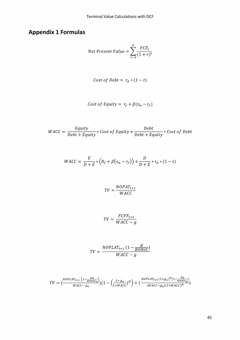
Terminal Value Calculations with DCF
45
Appendix 1 Formulas
𝑁𝑒𝑡 𝑃𝑟𝑒𝑠𝑒𝑛𝑡 𝑉𝑎𝑙𝑢𝑒 = ∑𝐹𝐶𝐹𝑡
(1 + 𝑟)𝑡
𝑛
𝑡−0
𝐶𝑜𝑠𝑡 𝑜𝑓 𝐷𝑒𝑏𝑡 = 𝑟𝑑 ∗ (1 − 𝑡)
𝐶𝑜𝑠𝑡 𝑜𝑓 𝐸𝑞𝑢𝑖𝑡𝑦 = 𝑟𝑓 + 𝛽(𝑟𝑚 − 𝑟𝑓)
𝑊𝐴𝐶𝐶 = 𝐸𝑞𝑢𝑖𝑡𝑦
𝐷𝑒𝑏𝑡 + 𝐸𝑞𝑢𝑖𝑡𝑦∗ 𝐶𝑜𝑠𝑡 𝑜𝑓 𝐸𝑞𝑢𝑖𝑡𝑦 +
𝐷𝑒𝑏𝑡
𝐷𝑒𝑏𝑡 + 𝐸𝑞𝑢𝑖𝑡𝑦∗ 𝐶𝑜𝑠𝑡 𝑜𝑓 𝐷𝑒𝑏𝑡
𝑊𝐴𝐶𝐶 = 𝐸
𝐷 + 𝐸∗ (𝑅𝑓 + 𝛽(𝑟𝑚 − 𝑟𝑓)) +
𝐷
𝐷 + 𝐸∗ 𝑟𝑑 ∗ (1 − 𝑡)
𝑇𝑉 =𝑁𝑂𝑃𝐴𝑇𝑡+1
𝑊𝐴𝐶𝐶
𝑇𝑉 = 𝐹𝐶𝐹𝐹𝑡+1
𝑊𝐴𝐶𝐶 − 𝑔
𝑇𝑉 = 𝑁𝑂𝑃𝐿𝐴𝑇𝑡+1 (1 −
𝑔𝑅𝑂𝑁𝐼𝐶)
𝑊𝐴𝐶𝐶 − 𝑔
𝑇𝑉 = (𝑁𝑂𝑃𝐿𝐴𝑇𝑡+1 (1−
𝑔𝑎𝑅𝑂𝑁𝐼𝐶𝑎
)
𝑊𝐴𝐶𝐶− 𝑔𝑎)(1 − (
1+ 𝑔𝑎
1+𝑊𝐴𝐶𝐶)𝑁) + (
𝑁𝑂𝑃𝐿𝐴𝑇𝑡+1(1+𝑔𝑎)𝑁(1−𝑔𝑏
𝑅𝑂𝑁𝐼𝐶𝑏)
(𝑊𝐴𝐶𝐶−𝑔𝑏)(1+𝑊𝐴𝐶𝐶)𝑁 )
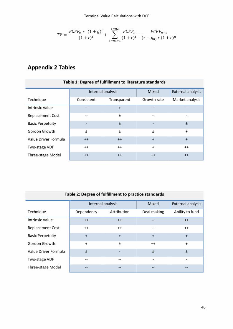
Terminal Value Calculations with DCF
46
𝑇𝑉 = 𝐹𝐶𝐹𝐹0 ∗ (1 + 𝑔)𝑡
(1 + 𝑟)𝑡+ ∑
𝐹𝐶𝐹𝐹𝑡
(1 + 𝑟)𝑡+
𝐹𝐶𝐹𝐹𝑛+1
(𝑟 − 𝑔𝑛) ∗ (1 + 𝑟)𝑛
𝑡=𝑛2
𝑡=𝑛1+1
Appendix 2 Tables
Table 1: Degree of fulfillment to literature standards
Internal analysis Mixed External analysis
Technique Consistent Transparent Growth rate Market analysis
Intrinsic Value -- + -- --
Replacement Cost -- ± -- -
Basic Perpetuity - ± - ±
Gordon Growth ± ± ± +
Value Driver Formula ++ ++ + +
Two-stage VDF ++ ++ + ++
Three-stage Model ++ ++ ++ ++
Table 2: Degree of fulfillment to practice standards
Internal analysis Mixed External analysis
Technique Dependency Attribution Deal making Ability to fund
Intrinsic Value ++ ++ -- ++
Replacement Cost ++ ++ -- ++
Basic Perpetuity + + + +
Gordon Growth + ± ++ +
Value Driver Formula ± - ± ±
Two-stage VDF -- -- - -
Three-stage Model -- -- -- --
Terminal Value Calculations with DCF
47
Appendix 3 Interview Questions (Dutch)
Interview vragenlijst Nederlands
De volgende vragen hebben betrekking op de praktijk berekening van de terminal value met een
DCF techniek.
Forecasted period
1: a) Hoewel het in feite geen effect hoort te hebben op de uiteindelijke waarde, over hoeveel jaar
berekend u normaalgesproken de explicit forecasted period? Houdt u hierbij rekening met de
investeringscyclus en de zogenaamde ‘steady-state’ hierop volgend?
b) wanneer wijkt u af van het bovengenoemde antwoord?
WACC
2 : a) U berekend en gebruikt een bepaalde WACC voor deze explicit forecasted period, in hoeverre
gebruikt u deze zelfde WACC in de berekening van de terminal period?
b) Hoe kijkt u aan tegen het gebruik van een ‘optimal structure’ als u kansen ziet voor verbetering
in de capital structure?
Terminal value:
Techniek:
3: a)Welke techniek past u toe bij het berekenen van een terminal value?
b) Wijkt u hier wel eens van af, zo ja, wanneer?
4: Welke drijfveren gebruikt u voor deze keuze?
5: Hoe bepaalt u een groei-prognose voor deze fase, en in welke orde van grootte liggen de
percentages die u in de groei heeft berekend?
6: Hoeveel wijkt deze gemiddeld genomen af van de groei die u meeneemt in de explicit forecasted
period?
7: In de literatuur zijn de meeste auteurs het erover eens dat een bedrijf niet sneller dan de
economie kan groeien in de terminal period (mathematisch zou het bedrijf dan op termijn groter
worden dan de economie) hoe kijkt u hier tegen aan?
8: Tussen 84 en 94 procent van de terminal value komt van de eerste 20 jaar in de terminal value
periode(Gordon Growth model met groei tussen 5 en 0 procent) (Rotkowski & Clough, 2013). Kunt u
zich voorstellen dat een bedrijf in zo’n periode een economie wél kan ‘outperformen’? (Hoe valide is
dan de vorige vraag/antwoord?)
9: Hoe kijkt u aan tegen een extra fase tussen de explicit forecasted en terminal period om de groei
geleidelijk af te laten nemen naar de stabiele waarde?
Terminal Value Calculations with DCF
48
10: Hoe kijkt u aan tegen de waarde van de terminal period relatief ten opzichte van de explicit
period, is deze te groot in uw ogen? (kan voor een high growth bedrijf oplopen tot boven 100% van
de waarde)
11: Denkt u dat het onvoorspelbare karakter van een terminal value berekening er voor zorgt dat u
wat conservatievere cijfers meeneemt in de berekening?
Algemeen
De komende vragen kunnen in meer of mindere mate een vergelijkbaar karakter hebben maar
hebben als doel om de rationele achter de gekozen technieken te begrijpen.
12: Heeft u het idee dat u voorál een ‘waarde’ of vooral een ‘overnameprijs’ berekend als u de
verkoop van een onderneming begeleid?
13: Hangt de berekening soms deels af van de situatie van de koper (of soms zelfs verkoper)?
14: Denkt u dat het construeren van een ‘mogelijke waarde’ (wanneer een bedrijf een betere
kapitaal structuur aanneemt) een goede aanvulling is voor het waarderingsrapport? Zijn hier ook
verschillen mogelijk naast de WACC?
15: In algemene zin, hoeveel van de waarde kunt u in uw ogen toeschrijven aan een verkopende
partij in geval van een overname, zit hem daarin ook het verschil tussen ‘waarde’ en ‘prijs’ in uw
ogen? En speelt hierbij de omvang van de onderneming een rol?