Elementary subpaths in discounted stochastic games

Kimmo Berg

Department of Mathematics and Systems Analysis, Aalto University School of Science, P.O.Box 11100, FI-00076 Aalto, Finland

Abstract

This paper examines the subgame-perfect equilibria in discounted stochasticgames with finite state and action spaces. The fixed-point characterizationof pure-strategy equilibria is generalized to unobservable mixed strategies. Itis also shown that the pure-strategy equilibria consist of elementary subpaths,which are repeating fragments that give the acceptable action plans in the game.The developed methodology offers a novel way of computing and analyzingequilibrium strategies that need not be stationary nor Markovian.

Keywords: game theory, stochastic game, subgame-perfect equilibrium,equilibrium path, fixed-point equation, tree

1. Introduction

Stochastic games are multiplayer decision making models in a dynamic en-vironment. They have been introduced in a seminal paper by Shapley (1953)and they can be applied, e.g., in industrial organization (Ericson and Pakes1995; Pakes and Ericson 1998), taxation (Phelan and Stacchetti 2001), fishwars, stochastic growth models, communication networks, queues, and hidingand searching for army forces; see the references in Filar and Vrieze (1997); Amir(2003); Doraszelski and Pakes (2007); Balbus et al. (2014). The stochastic gamemodel extends both Markov decision processes (MDPs) which have only a sin-gle decision maker and repeated games where the players encounter the samegame over and over again. In contrast to MDPs, the stochastic games may havemultiple solutions and a set of possible equilibrium payoffs that depends on theplayers’ strategies. Moreover, the strategies are inherently more complicatedcompared to repeated games as the actions can be planned conditionally basedon the realized future state.

This paper examines discounted stochastic games with a finite number ofplayers, actions and states. The existence of an equilibrium in stationary strate-gies has been proven in Fink (1964) and Takahashi (1964). For more generalstochastic games, the existence of an equilibrium is still an open problem. For

Email address: kimmo.berg@aalto.fi (Kimmo Berg)

Preprint submitted to - April 7, 2015

example, the stationary strategies may not be enough and the history-dependentbehavior strategies are needed when the state and the action spaces are moregeneral (Mertens and Parthasarathy 1987); see Levy (2013) and its corrigendum(Levy and McLennan 2015) for a game with no stationary nor Markovian equi-librium. Moreover, the indispensability of nonstationary (e.g., cyclic) strategiesand approximate equilibrium are typical features of stochastic games when thepayoffs are evaluated with the limiting average criterion (Blackwell and Fergu-son 1968; Flesch et al. 1997; Solan and Vieille 2001). This paper develops acomputational method for finding equilibria that need not be stationary norMarkovian, and this may help understand the solutions better that are requiredin more general stochastic games.

The pure-strategy subgame-perfect equilibria in repeated games has beencharacterized in Abreu (1986, 1988) and Abreu et al. (1986, 1990); we refer tothese paper by APS from now on. They show that it is enough to considersimple strategies and the extremal punishment paths support all equilibria1.The simple strategies define a path of actions that the players follow unless aunilateral deviation occurs. If this happens, the play switches regardless of thedeviation to the punishment path, which is the equilibrium path that gives theminimum payoff to the deviator. The same principles hold in stochastic games.The players follow a given plan of actions and the deviations are countered bythe player-specific punishments. However, the plan is no longer a deterministicpath but the actions and the punishments depend on the realized state. The factthat the players can condition their play on the state increases the complexityof the strategies and enlarges the set of equilibria compared to repeated games.It is also more difficult to derive monotonicity results for the equilibrium pathsand payoffs with respect to the players’ discount factors, since the equilibriumpayoffs are state dependent in general.

Abreu et al. (1986, 1990) have shown that the equilibrium payoffs can bedescribed with a set-valued fixed-point equation; Mertens and Parthasarathy(1987, 2003) give a resembling recursive presentation in stochastic games. TheAPS characterization has been generalized to stochastic games in several papers.Cole and Kocherlakota (2001) consider dynamic games with unobservable ac-tions and find that the set of Markov-private equilibria may be smaller than theset of pure-strategy sequential equilibria. Atkeson (1991) and Phelan and Stac-chetti (2001) develop recursive methods using a payoff relevant state variable.The folk theorem is proven in Fudenberg and Yamamoto (2011) and Horneret al. (2011), where they assume that the limit set is independent of the initialstate. Doraszelski and Escobar (2012) simplify the model by assuming that theplayers condition their play on summary statistics of past play and not the entirehistory. Kitti (2013b) examines a dynamic model with random disturbances andpure actions but assumes that they are both perfectly observed. Balbus et al.(2013) and Sleet and Yeltekin (2015) extend the methodology to uncountable

1See Thuijsman and Vrieze (1997); Flesch et al. (2000); Kitti (2013a) for the use of pun-ishment strategies in stochastic games.

2

state spaces, and Yamamoto (2015) studies a model with hidden states.In this paper, we develop a recursive characterization in behavior strategies

under the assumption that the players only observe the realized pure actions.This generalizes the result developed in repeated games (Berg and Schoenmakers2014). The mixed strategies impose an additional constraint that the differentcontinuation payoffs must be tailored so that the player is indifferent betweenthe pure actions in the support of the strategy.

The fixed-point characterization makes it possible to compute the set ofequlibria. The methods for repeated games under the simplifying assumption ofpublic correlation has been developed in Cronshaw (1997); Judd et al. (2003);Burkov and Chaib-draa (2010), which have been generalized to stochastic gamesin the following papers. MacDermed et al. (2011) present an algorithm for ap-proximating correlated equilibria that may not be subgame-perfect; see alsoMurray and Gordon (2007). Sleet and Yeltekin (2015); Yeltekin et al. (2015)compute correlated subgame-perfect equilibria that need not be Markovian us-ing lower and upper bounds. Balbus et al. (2014) provide a constructive methodfor finding stationary Markov strategies in uncountable state spaces where APStype methods may fail. Feng et al. (2014) find Markov equilibria in a model withshort-run players. The homotopy methods have also been extended to comput-ing stationary or Markov perfect equilibria in Herings and Peeters (2004); Govin-dan and Wilson (2009); Borkovsky et al. (2010); see also Judd et al. (2012) forcomputing all pure-strategy equilibria in continuous strategies, which is based onsolving all roots of polynomial equations (McKelvey and McLennan 1996; Datta2010). Lastly, Sen and Shanno (2008); Prasad et al. (2014) present optimizationformulations for finding stationary equilibria.

The APS characterization is a one-step method that considers only the cur-rent decision and all the future decisions and payoffs are embedded in the con-tinuation payoff. This paper focuses more on the players’ actions and developsa multi-step method where the players consider a sequence of actions, i.e., anaction plan that defines how the game is played in different future states. Theseaction plans can be represented as trees, and we construct pure-strategy equi-libria from the acceptable action plans. Berg and Kitti (2012) have developedthis idea in repeated games, where it is shown that the equilibrium paths con-sists of repeating fragments called elementary subpaths. These subpaths offera novel way of computing and analyzing the set of equilibria (Berg and Kitti2013, 2014). The pure-strategy payoffs can be identified as particular fractalscalled sub-self-affine sets and their density can be measured by the Hausdorffdimension. Furthermore, all the equilibrium paths can be represented with afinite graph when there are finitely many elementary subpaths and the size ofthe equilibrium set can be measured with the largest eigenvalue of the graph.

This paper generalizes this methodology to stochastic games. The factthat the equilibrium paths and the elementary subpaths are trees causes somechanges in the properties of equilibria. We observe that it is possible to plansome good payoffs in some contingencies in order to satisfy the incentive com-patibility conditions but leave some other contingencies without any plan. Ifthese unplanned states get, however, realized then all equilibria starting from

3

these states are possible as a continuation play. This property is named asregeneration effect since the planning of future actions can be restarted, andthis implies that the set of equilibria may be much larger compared to repeatedgames, where this cannot happen.

The paper is structured as follows. In Section 2, the stochastic game modeland the subgame-perfect equilibrium are defined. The set of equilibria is char-acterized in behavior strategies in Section 3. In Section 4, the equilibrium pathsare characterized in pure strategies, the elementary subpaths are generalized tostochastic games and an algorithm for producing the pure-strategy equilibriais presented. Numerical examples are examined in Section 5, where we observesome of the typical features of equilibrium behavior in stochastic games. Finally,Section 6 concludes.

2. Discounted stochastic games

We examine a stochastic game defined by a finite set of states and a normal-form game played at each state. The transitions between the states depend onthe players’ actions. In each period, the players receive payoffs from the currentgame and they observe the current state and all the past pure actions beforemaking their choices. This process is repeated infinitely and the players discountthe future payoffs.

A finite discounted stochastic game is defined by the tuple (N,S,A, u, δ),where

• N = {1, . . . , n} is the finite set of players,

• S = {1, . . . ,m} is the finite set of states,

• Asi is the finite set of pure actions for player i ∈ N in state s ∈ S and

As = ×i∈NAsi is the set of pure action profiles. A pure action of player i

is called ai ∈ Asi and a pure action profile is called a ∈ As.

• u(s, a) ∈ Rn is the vector of players’ payoffs for action profile a ∈ As instate s ∈ S,

• δi ∈ [0, 1) is the discount factor of player i ∈ N .

To simplify the notation, it is assumed that the players have the same numberof actions in each state, i.e., A = As for all s ∈ S, and they have the samediscount factors δ = δi for all i ∈ N .

The game begins in an initial state s1 ∈ S and the state evolves based onthe players’ latest actions, i.e., there is a time-independent transition functionq : S × A 7→ ∆(S), where ∆(S) is the set of probability distributions over S.The probability of reaching state t after state s and an action profile a ∈ A isdenoted by q(t|s, a) and naturally

∑t∈S q(t|s, a) = 1 for all s ∈ S and a ∈ A.

The distribution over the initial states is given by q(∅).In each period, player i ∈ N may randomize over his pure actions ai ∈

Ai, which gives a mixed action zi so that zi(ai) ≥ 0 for each ai ∈ Ai and

4

∑ai∈Ai

zi(ai) = 1. The set of probability distributions over Ai is called Zi =∆(Ai) and Z = ×i∈NZi. A mixed action profile is denoted by z = (z1, . . . , zn) ∈Z. We also denote the mixed action in state s by zs. The support of a mixed ac-tion is the set of pure actions that are played with a strictly positive probability,i.e., Supp(zi) = {ai ∈ Ai|zi(ai) > 0}. We also define Supp(z) = ×i∈NSupp(zi)and for each a ∈ Supp(z), we let πz(a) be the probability that action profile ais realized if the mixed action profile z is played: πz(a) =

∏j∈N zj(aj). The

player i’s opponents’ action profile is denoted by z−i ∈ Z−i = ×j∈N,j =iZj .The payoffs in each period are given by the function u : S ×Z 7→ Rn. If the

players use a mixed action profile z ∈ Z in state s ∈ S then player i receives anexpected payoff of

ui(s, z) =∑a∈A

ui(s, a)πz(a). (1)

We also denote ui(s, z) = ui(zs) to shorten the notation.

The players only observe the realized pure actions and not the randomiza-tions that the other players are using. They also observe the current state beforemaking their decisions and have perfect recall, i.e., they remember all the paststates and the pure action profiles. Thus, the public past play is given by the setof histories Hk = Hk−1 ×A× S and the initial set of histories at the beginningof the game is H1 = S. The set of all histories is H = ∪k≥1H

k.A behavior strategy of player i is a mapping σi : H 7→ Zi, which assigns a

mixed action in the current state for each possible history in the game. The setof strategies of player i is Σi. A strategy profile σ = ×i∈Nσi is the composition ofthe players’ strategies and the set of strategy profiles is Σ = ×i∈NΣi. The playeri’s opponents’ strategy profile is denoted by σ−i = ×j∈N,j =iσj and similarlyΣ−i = ×j∈N,j =iΣj . A pure strategy selects deterministically one of the pureactions, i.e., a pure strategy is a mapping σi : H 7→ Ai.

The players discount the future payoffs with a discount factor δ ∈ [0, 1). Theexpected discounted payoff of player i from a strategy profile σ is

Ui(σ) = Eσ

[(1− δ)

∞∑k=1

δk−1ui(sk, zk)

], (2)

where the expectation is over the histories induced by the distribution of initialstate q(∅) and σ, sk is the induced state at period k and zk is the inducedmixed action profile for the given history.

A strategy profile σ is a Nash equilibrium if no player has a profitable devi-ation, i.e.,

Ui(σ) ≥ Ui(σ′i, σ−i), for all i ∈ N and σ′

i ∈ Σi. (3)

A strategy profile σ is a subgame-perfect equilibrium (SPE) if it induces aNash equilibrium in every subgame, i.e., for any history h ∈ H ending in states, the continuation strategy induced by history h, denoted by σ|h, is a Nashequilibrium of the continuation game starting from the state s:

Ui(σ|h) ≥ Ui(σ′i, σ−i|h), for all i ∈ N , h ∈ H and σ′

i ∈ Σi. (4)

From now on, equilibrium refers to a subgame-perfect equilibrium.

5

3. Characterization of equilibrium

Let V ⊂ Rn×m be the set of SPE payoffs in the stochastic game. A vectorfrom this set gives a payoff for each player and state. We denote the payoffs instate s by V (s), i.e., v(s) = (vs1, . . . , v

sn) ∈ V (s) and v = (v(1), v(2), . . . , v(m)) ∈

V . Moreover, V (δ) refers to the payoff set with the discount factor δ. Theminimum payoff of player i in state s from a non-empty compact set W ⊂ Rn×m

is denoted byv−i (s,W ) = min {vi : v ∈W (s)} . (5)

The minimum equilibrium payoff in state s is denoted by v−i (s) = v−i (s, V ).This is the payoff that the player receives if he deviates and the game evolvesto state s since there is a transition before the deviation is observed.

Suppose that the players use a mixed action profile z in state s ∈ S andthere is a compact set of continuation payoffs W = (W (1), . . . ,W (m)). Thecontinuation play can be set distinctively for each pair (as, t) of an action pro-file a ∈ Supp(zs) and a future state t ∈ S such that the players receive acontinuation payoff x(a, t) ∈W (t). The expected continuation payoff is

w =∑t∈S

∑a∈Supp(z)

πz(a)q(t|s, a)x(a, t). (6)

Now, a pair (zs, w) consisting of an action profile z in state s and an expectedcontinuation payoff w is admissible with respect to W if it satisfies the incentivecompatibility (IC) conditions

(1− δ)ui(zs) + δwi ≥ max

a′i∈Ai\Supp(zi)

[(1− δ)ui(a

′i, z−i) + δvc−i ((a′i, z−i),W )

],

(7)for all i ∈ N , where vc−i (zs,W ) is the punishment continuation payoff of playeri from W in state s after an action profile zs

vc−i (zs,W ) =∑t∈S

∑a∈Supp(z)

πz(a)q(t|s, a)v−i (t,W ). (8)

When player i deviates to the action profile zs, the sum goes through all thepossible pure action profiles in the support and all the possible future statesgiven these pure actions. For each possible future state t, the play is followed bythe punishment payoff in that state v−i (t,W ). The IC conditions mean that it isbetter for player i to take a mixed action zsi and get the expected continuationpayoff wi than to deviate and obtain the punishment continuation payoffs. Notethat in Eq. (7) the maximum deviation may not be obtained with the actionthat gives the highest instant payoff since the transitions and the future states(and thus the total punishment payoff) may be different after each pure actionprofile.

Let Ms(x) denote the set of all equilibrium payoffs in state s ∈ S in a stagegame with payoffs u(a)

.= (1 − δ)u(s, a) + δx(a) for an action profile a ∈ As,

wherex(a) =

∑t∈S

q(t|s, a)x(a, t).

6

For each pure action profile a ∈ As, we have a continuation payoff x(a, t) foreach possible future state t, i.e., possibly m different continuation payoff vectors.With |A| different pure action profiles, the vector x has m × |A| continuationpayoff vectors.

Let us define a mapping B : Rn×m → Rn×m

B(W ) = (B1(W ), . . . , Bm(W )), (9)

whereBs(W ) =

∪x(a,t)∈W (t)

(z,w) IC w.r.t. W

Ms(x), (10)

s ∈ S, a ∈ As, w =∑

t∈S

∑a∈Supp(z) πz(a)q(t|s, a)x(a, t), (z, w) is admissible

with respect to W and z is an equilibrium in the stage game in state s ∈ Sdefined by the continuation payoffs x ∈ Wm×|A|. A set W is self-generating ifW ⊆ B(W ). The main theorem follows directly from the next proposition.

Proposition 1. Suppose a bounded set W is self-generating then B(W ) ⊆ V .

Proof. It is enough to show that for all payoffs v ∈ B(W ) there is a strategy thatproduces the payoff and that strategy does not have any unilateral deviationsat any period. We construct a sequence of strategies from the stage game Nashequilibria. We examine a payoff v(s) ∈ Bs(W ) in state s ∈ S. This meansthat v(s) ∈ Ms(x), x ∈ Wm×|A|, i.e., there is a Nash equilibrium with a mixedaction z1 which gives a payoff v(s) from the stage game where the payoffs takeinto account all the future payoffs and the continuation payoffs are drawn fromthe set W . There are no profitable deviations on the first period as the play isgiven by a Nash equilibrium in the stage game. Since the continuation payoffsare drawn from the same set W , there are no profitable deviations in the futureperiods either as the same holds for any payoff in B(W ) in any state. In the firstperiod, the players play z1 and then a pure action profile a ∈ Supp(z1) is realizedand the game evolves into state t. Now, the players need to produce a payoffx(a, t) in the second period. Since x(a, t) ∈ W (t) and W is self-generating, wehave x(a, t) ∈ Bt(W ). In similar way, there is a mixed action z2 that is Nashequilibrium, has no profitable deviations and produces the payoff x(a, t). Byrepeating this iteration, we produce a sequence of mixed actions (z1, z2, . . .)with no profitable deviations that produce the expected payoff v.

Theorem 1. The payoff set V is the largest fixed point of W = B(W ).

Note that it can be shown that the payoff set V is compact, which followsfrom the finiteness of stage game payoffs and states. It can also be shown thatthe self-generating sets are monotone in δ if they are convex and the payoffsproduced in different states overlap.

Proposition 2. Suppose a bounded set W ⊂ Rn is convex and Wm = (W, . . . ,W ) ⊆ V (δ1) is a self-generating set then Wm ⊆ V (δ2) for δ2 ≥ δ1.

7

Proof. It is enough to show that the same stage game payoffs can be constructedwith δ2 that are used in the equilibrium strategies with δ1 and the admissibilityis not violated. We need to show that we can find continuation payoffs x2(a, t) ∈W (t) such that u(a) = (1− δ1)u(s, a) + δ1x

1(a) = (1− δ2)u(s, a) + δ2x2(a). By

denoting δ2 = δ1 + ϵ, we get (δ1 + ϵ)x2(a) = δ1x1(a) + ϵu(s, a). We get this

x2(a) by selecting for each (δ1 + ϵ)x2(a, t) = δ1x1(a, t) + ϵu(s, a). From the

above equations, we get that x2(a, t) is between x1(a, t) and u(a). This meansthat x2(a, t) ∈W (t) as x1(a, t) ∈W (t), u(a) ∈W (t) and W (t) is convex.

Note that, contrast to repeated games, it is not enough for the payoff mono-tonicity that the self-generating sets W (s), s ∈ S, are convex. For example,take a game with two states and all the transitions are deterministic to state2. Suppose that there is a single Nash equilibrium in both of the states, whosepayoff is not the same. Let us denote these payoffs by u1 and u2. Then the onlyequilibrium payoff in state 1 is (1− δ)u1 + δu2. This keeps changing no matterhow large the discount factor is and thus the payoff set is not monotone in δ.Thus, it is more difficult to obtain payoff monotonicity in stochastic games.

4. Equilibrium paths in pure strategies

The construction of pure-strategy equilibria can be seen as a problem ofdesigning a sequence of pure action profiles such that no player wishes to deviatefrom the plan. Since the state transitions are probabilistic, the actions areplanned conditional on the realized state. This plan of conditional actions iscalled as a path or a tree, which is defined as follows.

A path p defines a pure action profile for the current state and all the possiblefuture states that are reachable when the players follow the path. The length ofpath p is the maximum depth how far the actions are planned in the future. Forexample, if |p| = 1 then the path defines the action profile only to the currentperiod (one action profile) and if |p| = 2 then the path defines the action profilesto the current period (one action profile) and the next period (possibly up tom action profiles). A path is called perfect if it defines the action profiles up tothe same length in all contingencies. To simplify the notation, we only considerperfect paths in this paper and assume that all the states are reachable fromany state after any action profile.

The action profiles on the path are numbered as follows: pk,j refers to thejth action profile on the kth period. The numbering is illustrated in Fig. 1(a),which shows a path of length three starting from state 1 in a game with threestates. For example, p1,1 = a1 is the root action profile, which is played on thecurrent period, p2,3 = d3 is the action profile played on the second period instate 3 and p3,8 = c2 is played in the third period in state 2 (if the state is 3 inthe second period). With a perfect path p, we have 1 ≤ j ≤ mk−1 and the pathhas a total of (m|p| − 1)/(m− 1) action profiles.

A subpath or a subtree is a part of a path. For example, taking a subpathmeans selecting a node in the tree and picking all or some of its descendants (sothat the selected nodes form a tree). Let sub(pk,j) denote the subpath starting

8

from node pk,j and picking all of its descendants. For example, sub(p2,3) containsp2,3 = d3 as the root node and p3,7 = c1, p3,8 = c2 and p3,9 = b3 as its children.Moreover, start(p, k), k ≤ |p|, denotes the action profiles of the path up tolength k. For example, start(p, 2) contains the actions on the first two periods.

Let p(σ) denote the infinite path induced by a strategy σ and v(pk,j) is thecontinuation payoff on path p after the action profile r = pk,j defined recursively:

v(r) =∑t∈S

q(t|r)[u(t, sub(r2,t)) + δv(sub(r2,t))

],

where sub(r2,t) is the action profile in state t after r. The following result showsthat the equilibrium paths do not have any profitable deviations.

Proposition 3. A path p is an equilibrium path induced by a pure-strategy σ ifand only if

(1−δ)ui(pk,j(σ))+δvi(p

k,j(σ)) ≥ maxa′i∈As

i

[(1− δ)ui(a

′i, p

k,j−i (σ)) + δvc−i ((a′i, p

k,j−i (σ)), V )

],

(11)for all i ∈ N , k ≥ 1 and 1 ≤ j ≤ mk−1.

Proof. The proof follows from Proposition 2.2.1 in Mailath and Samuelson(2006). The main idea is to show that the discounting implies that a strat-egy with a higher payoff must produce this higher payoff within a finite numberof periods. In stochastic games, the future payoffs can be bounded by payoffs

δk(maxs∈S

maxa∈As

ui(s, a)−mins∈S

mina∈As

ui(s, a)).

Eqs. (11) are called the incentive compatibility (IC) conditions. They meanthat at any stage of the SPE path all the players prefer taking the actionsprescribed by the SPE strategy σ, rather than deviating and then receiving theminimum equilibrium payoffs. The exhausting task of going through all thepossible realizations of the stochastic path can be further simplified by findingfinite fragments of which the SPE paths consists of and these fragments will becalled the elementary subpaths; this will be shown in Section 4.1.

As in repeated games, it is enough to consider only the simple strategieswhen studying the equilibrium outcomes. A simple strategy is defined by n ×m + 1 paths (p0, p1,1, . . . , pn,m): an initial path p0 that the play follows and apunishment path pi,s for each player i ∈ N and for each state s ∈ S. The playfollows the current path unless there is a unilateral deviation. In this case, theplay switches to the punishment path of the deviator in the future state. If morethan one player deviates, the play stays on the current path. These deviationscan be neglected in non-cooperative games.

Proposition 4. A path p can be supported as an outcome of a pure-strategyequilibrium if and only if there are n×m punishment paths pi,s, i ∈ N , s ∈ S,such that the simple strategy (p, p1,1, . . . , pn,m) is an equilibrium.

9

Proof. Suppose p is an outcome of a pure-strategy equilibrium. This means thatthe path does not have any profitable unilateral deviations. Since the punish-ment paths give by definition the minimum equilibrium payoffs, the incentivecompatibility conditions also hold when the deviations on the path are followedby the punishment paths, instead of the ones defined by the pure-strategy equi-librium. Thus, the simple strategy is an equilibrium.

4.1. Elementary subpaths

We now demonstrate through examples how the elementary subpaths ofrepeated games generalize to stochastic games.

Example 1. In a repeated game with four action profiles, we denote the actionprofiles by letters a to d. Let us assume that the elementary subpaths of thegame are d, aa, bc, ba, cb and ca. The elementary subpaths are fragmentsthat can be played in the game as long as they are followed by any equilibriumpath starting from the final action profile on the subpath. The subpaths areconstructed in such a way that the incentive compatiblity conditions are satisfiedalong the subpath. For example, a path (bc)∞ = bcbcbc . . ., where (bc)∞ denotesthe infinite repetition of bc, is an equilibrium path since it consists of combiningthe elementary subpaths bc and cb. Also, paths a∞, d∞, bca∞ and ddddbcbcba∞

are equilibrium paths as they are composed of the elementary subpaths. Bergand Kitti (2012, 2013) show how to get all the equilibrium paths and representthem with a graph when there are finitely many elementary subpaths.

The stochastic games are a bit more complicated as the continuation pathsare not deterministic and the game may evolve to multiple future states. Theequivalent concept of an elementary subpath in stochastic games is a tree, whichdefines action profiles for some future states. Fig. 1a shows a three-length pathin a stochastic game with three states, compared to a repeated game path acbshown below. Instead of having one action profile for each future period, theremay be one action profile for each possible future state. The tree is perfect asit defines the actions for all the possible realizations in the first three periods.

Fig. 1b shows how to construct a stochastic equilibrium path from theelementary subpaths in a game with two states. The star in d∗ denotes that theaction d can be played in any of the states, i.e., d∗ corresponds to two paths d1

and d2, which shortens the list of paths. The idea is to combine the elementarysubpaths in a proper manner so that all the action profiles fit together and allthe incentive compatibility conditions are satisfied. The first action p1,1 = d1

in the root node is incentive compatible, since d∗, i.e., both d1 and d2 areelementary subpaths; this is shown with a small dashed box. The second periodactions p2,1 = b1 and p2,2 = c2 are also IC, since their continuation actions fitthe elementary subpaths bcc and cab , respectively. In the third period, the figureshows two elementary subpaths caa and bcc with dashed boxes, which means thatboth p3,1 = c1 and p3,4 = b2 are IC. Since all the actions on the path are IC,the shown path is a viable start and a subpath for an equilibrium path in thestochastic game.

10

a1

c1

b1

a2

b3

a2

b1

d2

c3

d3

c1

c2

b3

k = 1 k = 2 k = 3

a c b

Elementary subpaths

d∗ b∗a1

a2

b∗a1

c2

b∗c1

c2

a∗a1

a2

c∗a1

a2

c∗a1

b2

c∗b1

b2

d1

b1

c1a1

a2

c2a1

b2

c2

a1a1

a2

b2c1

c2

(a) Comparison of paths (b) Construction of equilibrium path

Figure 1: Elementary subpaths and constructing an equilibrium path with them.

11

Now, let us define the concept formally. Let con(s, a) denote the minimumcontinuation payoff that is required to make an action profile a ∈ As incentivecompatible in state s:

(1− δ)ui(s, a) + δconi(s, a) = maxa′i∈As

i

[(1− δ)ui(a

′i, a−i) + δvc−i ((a′i, a−i), V )

].

(12)We also denote con(as) = con(s, a). Let u(p) denote the expected payoff of aperfect finite path p

ui(p) = ui(p1,1) +

|p|∑k=2

δk−1mk−1∑j=1

q(pk,j)ui(pk,j), (13)

where i ∈ N and q(pk,j) is the probability of reaching node pk,j . The maximumpayoff of player i in state s is

v+i (s) = max {vi : v ∈ V (s)} , (14)

and the maximum continuation payoff after an action profile a ∈ As is

vc+i (s, a) =∑t∈S

q(t|s, a)v+i (t). (15)

Since the minimum and maximum payoffs are typically not known in ad-vance, they can be approximated with the following lower and upper bounds.For a lower bound, we can find the fixed-points of

v−i (s) = mina−i∈As

−i

maxai∈As

i

(1− δ)ui(ai, a−i) + δ∑t∈S

q(t|s, (ai, a−i))v−i (t), (16)

and the starting values can be the minimum minimax payoffs over the states.We leave for future research how the minimum payoffs should be found. It isnot an easy task even in repeated games (Berg 2013; Berg and Karki 2014a),but these methods can be generalized to stochastic games. For an upper bound,we can solve

v+i (s) = maxa∈A

(1− δ)ui(a) + δ∑t∈S

q(t|s, a)v+i (t), (17)

and the starting values can be the maximum stage game payoffs over the states.The values v+(s) affect how fast Algorithm 1 converges.

A path is first-action feasible (FAF) if the first action profile (the root node)is incentive compatible when the path is continued by any equilibrium path.

Definition 1. A perfect path p, starting with an action a ∈ As in state s, is anFAF path if

(1−δ)ui(p)+δ|p|m|p|−1∑j=1

q(p|p|,j)coni(p|p|,j) ≥ max

a′i∈As

i

[(1− δ)ui (a

′i, a−i) + δvc−i ((a′i, a−i), V )

],

(18)for all i ∈ N .

12

The one-length FAF paths have no profitable deviations and these actionprofiles maximize the right hand-side of the incentive compatibility conditionfor all players. Note that the FAF paths may have profitable deviations fromthe other action profiles than the root node.

Similarly, it is possible to find the paths that cannot be FAF and these arecalled the first-action infeasible (FAI) paths.

Definition 2. A perfect path p, starting with an action a ∈ As in state s, is anFAI path if

(1−δ)ui(p)+δ|p|m|p|−1∑j=1

q(p|p|,j)vc+i (p|p|,j) < maxa′i∈As

i

[(1− δ)ui (a

′i, a−i) + δvc−i ((a′i, a−i), V )

],

(19)for any i ∈ N .

The definition means that the FAI path is not incentive compatible no matterwhat equilibrium path follows it. Thus, the FAI paths cannot be a part of anyequilbrium path.

The paths can now be classified into FAF, FAI or neutral (N) paths, whichare neither FAF nor FAI. We are only interested in the shortest FAF or FAIpaths for the following reason. Suppose a path p is an FAF (FAI) path thenany longer path starting with p and continuing it with any equilibrium pathis also an FAF (FAI) path. A path is called minimal if it is the shortest pathin satisfying certain conditions. Now, we are ready to define the elementarysubpaths.

Definition 3. A perfect path p is an elementary subpath if it is minimal FAFpath and all of its subpaths are covered by some FAF paths: for all 1 ≤ k ≤ |p|and 1 ≤ j ≤ mk−1 either part(sub(pk,j), i) is an FAF path for some 1 ≤ i ≤|sub(pk,j)| or sub(pk,j) = part(q, |sub(pk,j)|) for some FAF path q.

The second condition requires that all of the action profiles on the pathneed to be incentive compatible. In the first case, when part(sub(pk,j), i) isan FAF path for some 1 ≤ i ≤ |sub(pk,j)|, the path itself guarantees that theaction profile is IC. In the second case, when sub(pk,j) = part(q, |sub(pk,j)|)for some FAF path q, the path may need to be continued with some actionprofiles in order to make some of its action profiles IC. Note that it is possiblethat the elementary subpaths are infinitely long in which case they are actuallyequilibrium paths. Essentially, the elementary subpaths are FAF paths that donot have profitable deviations at any node. The following result shows that theequilibrium paths consist of elementary subpaths.

Proposition 5. A path p is an equilibrium path if and only if all of its sub-paths are covered by elementary subpaths: for all k ≥ 1 and 1 ≤ j ≤ mk−1

part(sub(pk,j), i) is an elementary subpath for some i ≥ 1.

Proof. Suppose all of the subpaths of a path is covered by elementary subpaths.This means that the incentive compatibility conditions are satisfied for all action

13

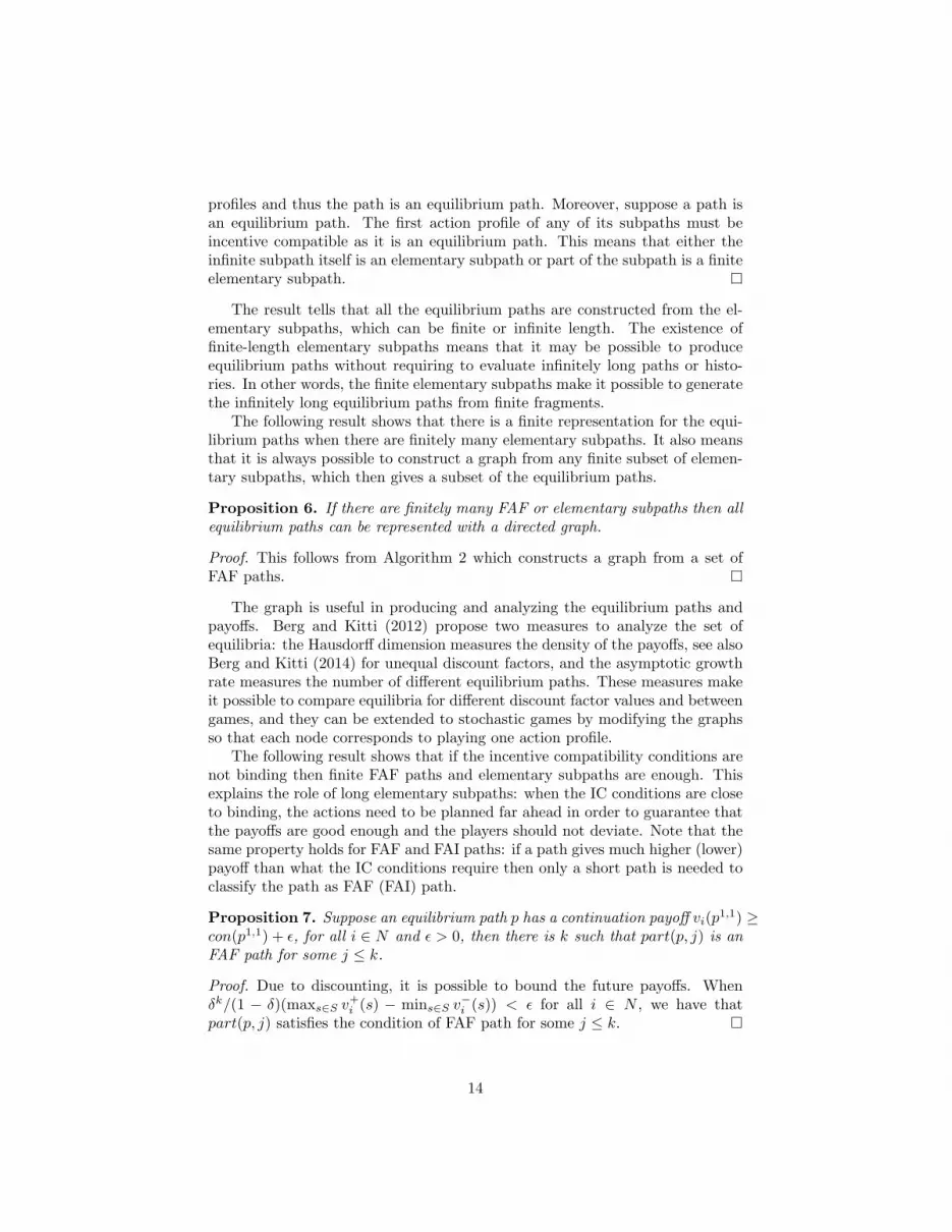
profiles and thus the path is an equilibrium path. Moreover, suppose a path isan equilibrium path. The first action profile of any of its subpaths must beincentive compatible as it is an equilibrium path. This means that either theinfinite subpath itself is an elementary subpath or part of the subpath is a finiteelementary subpath.

The result tells that all the equilibrium paths are constructed from the el-ementary subpaths, which can be finite or infinite length. The existence offinite-length elementary subpaths means that it may be possible to produceequilibrium paths without requiring to evaluate infinitely long paths or histo-ries. In other words, the finite elementary subpaths make it possible to generatethe infinitely long equilibrium paths from finite fragments.

The following result shows that there is a finite representation for the equi-librium paths when there are finitely many elementary subpaths. It also meansthat it is always possible to construct a graph from any finite subset of elemen-tary subpaths, which then gives a subset of the equilibrium paths.

Proposition 6. If there are finitely many FAF or elementary subpaths then allequilibrium paths can be represented with a directed graph.

Proof. This follows from Algorithm 2 which constructs a graph from a set ofFAF paths.

The graph is useful in producing and analyzing the equilibrium paths andpayoffs. Berg and Kitti (2012) propose two measures to analyze the set ofequilibria: the Hausdorff dimension measures the density of the payoffs, see alsoBerg and Kitti (2014) for unequal discount factors, and the asymptotic growthrate measures the number of different equilibrium paths. These measures makeit possible to compare equilibria for different discount factor values and betweengames, and they can be extended to stochastic games by modifying the graphsso that each node corresponds to playing one action profile.

The following result shows that if the incentive compatibility conditions arenot binding then finite FAF paths and elementary subpaths are enough. Thisexplains the role of long elementary subpaths: when the IC conditions are closeto binding, the actions need to be planned far ahead in order to guarantee thatthe payoffs are good enough and the players should not deviate. Note that thesame property holds for FAF and FAI paths: if a path gives much higher (lower)payoff than what the IC conditions require then only a short path is needed toclassify the path as FAF (FAI) path.

Proposition 7. Suppose an equilibrium path p has a continuation payoff vi(p1,1) ≥

con(p1,1) + ϵ, for all i ∈ N and ϵ > 0, then there is k such that part(p, j) is anFAF path for some j ≤ k.

Proof. Due to discounting, it is possible to bound the future payoffs. Whenδk/(1 − δ)(maxs∈S v+i (s) − mins∈S v−i (s)) < ϵ for all i ∈ N , we have thatpart(p, j) satisfies the condition of FAF path for some j ≤ k.

14

Algorithm 1: Breadth-first search to classify the finite paths.

input : u, v−, v+, q, δ and maximum path length.output: FAF, FAI and N paths up to the given path length.define: comb(p) gives all combinations of paths starting with p, whenthe length is increased by one. This involves picking all thecombinations of m|p| action profiles from the sets As.

beginSet queue counter i = 1.for s← 1 to m do

for j ∈ As doif con(as(j)) ≤ v−(as(j)) then as(j) is an FAF path.else if con(as(j)) ≥ v+(as(j)) then as(j) is an FAI path.else add paths comb(as(j)) to queue q.

while |q(i)| ≤ maximum path length doif q(i) satisfies Eq. (18) then q(i) is an FAF path.else if q(i) satisfies Eq. (19) then q(i) is an FAI path.else add paths comb(q(i)) to queue q.if end of queue then Stop.Otherwise, set i = i+ 1.

Let us define a strict equilibrium by the paths that satisfy the IC conditionsin Eq. (11) with a strict inequality along the path. The previous result togetherwith Proposition 6 then implies:

Proposition 8. The set of strict equilibrium is finite.

4.2. Computational method

The following methods are modified from the ones in repeated games (Bergand Kitti 2012, 2013). Algorithm 1 finds the finite-length FAF and FAI paths.Algorithm 2 shows how to get the elementary subpaths from the FAF pathsand how to form a graph presentation for the equilibrium paths. Example 2illustrates how the algorithm works.

Example 2. Let us assume that the FAF paths of a two-state game are the onesgiven in Fig. 2; they are numbered T1-T3 on the first line and T4-T7 on thesecond line. The FAF path T4 has an infeasible subpath, which is shown with adashed box. There is no FAF path that starts with b1 and then continues withb1 in state 1 and c2 in state 2 and thus FAF path T4 cannot be an elementarysubpath. All the other FAF paths are elementary, since they are minimal and alltheir subpaths are covered by some FAF paths. Algorithm 2 is now demonstratedwith these FAF paths.

In Step 1, a tree of the FAF paths is created. This is shown in Fig. 3a andit is called the supertree ST. For example, the FAF path T5 is added to ST in

15

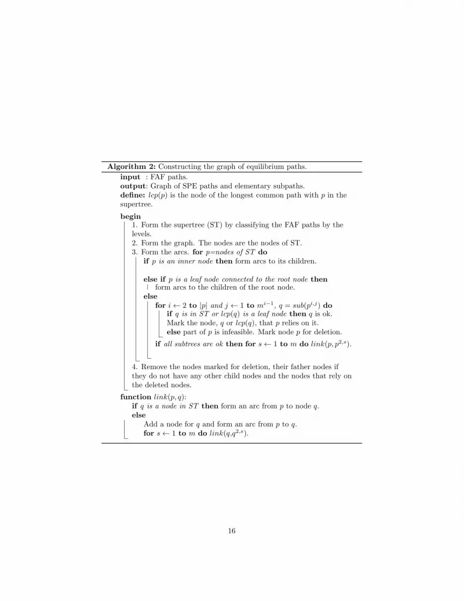
Algorithm 2: Constructing the graph of equilibrium paths.

input : FAF paths.output: Graph of SPE paths and elementary subpaths.define: lcp(p) is the node of the longest common path with p in thesupertree.

begin1. Form the supertree (ST) by classifying the FAF paths by thelevels.2. Form the graph. The nodes are the nodes of ST.3. Form the arcs. for p=nodes of ST do

if p is an inner node then form arcs to its children.

else if p is a leaf node connected to the root node thenform arcs to the children of the root node.

elsefor i← 2 to |p| and j ← 1 to mi−1, q = sub(pi,j) do

if q is in ST or lcp(q) is a leaf node then q is ok.Mark the node, q or lcp(q), that p relies on it.else part of p is infeasible. Mark node p for deletion.

if all subtrees are ok then for s← 1 to m do link(p, p2,s).

4. Remove the nodes marked for deletion, their father nodes ifthey do not have any other child nodes and the nodes that rely onthe deleted nodes.

function link(p, q):if q is a node in ST then form an arc from p to node q.else

Add a node for q and form an arc from p to q.for s← 1 to m do link(q,q2,s).

16

T1

a∗a1

a2

T2

c∗a1

a2

T3

c∗b1

b2

T4

a∗

b1b1

c2

c2b1

b2

T5

a1

b1c1

c2

c2b1

b2

T6

b∗

c1a1

a2

c2a1

a2

T7

b∗

c1b1

b2

c2b1

b2

Figure 2: Checking the subpaths of FAF paths.

∅

a1

T1 b1

c2

T4 T5

a2

T1 b1

c2

T4

c∗

T2 T3

b∗

c1

c2

T6 T7

a2 a1

∅ c∗ T3

b∗ c1

c2 T2

T7 T6

(a) Supertree (b) Graph of equilibrium paths

Figure 3: Forming the supertree and the graph.

17

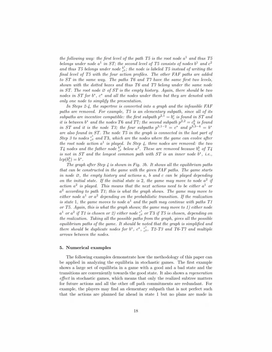
the following way: the first level of the path T5 is the root node a1 and thus T5belongs under node a1 in ST; the second level of T5 consists of nodes b1 and c2

and thus T5 belongs under node b1

c2 ; the node is labeled T5 instead of writing thefinal level of T5 with the four action profiles. The other FAF paths are addedto ST in the same way. The paths T6 and T7 have the same first two levels,shown with the dotted boxes and thus T6 and T7 belong under the same nodein ST. The root node ∅ of ST is the empty history. Again, there should be twonodes in ST for b∗, c∗ and all the nodes under them but they are denoted withonly one node to simplify the presentation.

In Steps 2-4, the supertree is converted into a graph and the infeasible FAFpaths are removed. For example, T5 is an elementary subpath, since all of itssubpaths are incentive compatible: the first subpath p2,1 = bcc is found in ST andit is between b∗ and the nodes T6 and T7; the second subpath p2,2 = cbb is foundin ST and it is the node T3; the four subpaths p3,1−2 = c∗ and p3,3−4 = b∗

are also found in ST. The node T5 in the graph is connected in the last part ofStep 3 to nodes c1

c2 and T3, which are the nodes where the game can evolve afterthe root node action a1 is played. In Step 4, three nodes are removed: the twoT4 nodes and the father node b1

c2 below a2. These are removed because bbc of T4is not in ST and the longest common path with ST is an inner node b∗, i.e.,lcp(bbc) = b∗.

The graph after Step 4 is shown in Fig. 3b. It shows all the equilibrium pathsthat can be constructed in the game with the given FAF paths. The game startsin node ∅, the empty history and actions a, b and c can be played dependingon the initial state. If the initial state is 2, the game may move to node a2 ifaction a2 is played. This means that the next actions need to be either a1 ora2 according to path T1; this is what the graph shows. The game may move toeither node a1 or a2 depending on the probabilistic transition. If the realizationis state 1, the game moves to node a1 and the path may continue with paths T1or T5. Again, this is what the graph shows; the game may move to 1) either node

a1 or a2 if T1 is chosen or 2) either node c1

c2 or T3 if T5 is chosen, depending onthe realization. Taking all the possible paths from the graph, gives all the possibleequilibrium paths of the game. It should be noted that the graph is simplified andthere should be duplicate nodes for b∗, c∗, c1

c2 , T2-T3 and T6-T7 and multiplearrows between the nodes.

5. Numerical examples

The following examples demonstrate how the methodology of this paper canbe applied in analyzing the equilibria in stochastic games. The first exampleshows a large set of equilibria in a game with a good and a bad state and thetransitions are conveniently towards the good state. It also shows a regenerationeffect in stochastic games, which means that only the realized subtree mattersfor future actions and all the other off path commitments are redundant. Forexample, the players may find an elementary subpath that is not perfect suchthat the actions are planned far ahead in state 1 but no plans are made in

18

state 2. Now, if the game evolves to state 2, the game may proceed with all thepossible equilibrium paths starting from state 2. The second example shows howthe equilibria in stochastic games differ from the equivalent game in repeatedgames. This example suggests that the sets of equilibria are much larger instochastic games in general.

5.1. Two prisoner’s dilemmas

This game has been examined in Kitti (2013b). There are two states with adifferent prisoner’s dilemma game in each. The letters a to d refer to the actionprofiles (T, L), (T,R), (B,L) and (B,R), respectively.

state 1L R

T 4,4 # 0,5 #

B 5,0 # 1,1state 2

L RT 0,0 -4,1B 1,-4 -3,-3 #

The discount factor is δ = 0.45 and the transition probabilities are q(1|1, a−c) =q(2|2, d) = 1 and q(1|1, d) = q(2|2, a−c) = 0.5. The symbol # marks the actionsafter which the state stays deterministically the same.

The first step is to find the minimum equilibrium payoffs and the punishmentpaths. The value δ = 0.4 is the limit when the punishment path changes fromrepeating the Nash equilibria d∗, with payoffs 1 and -3, to repeating actionsb∗ (c∗) when player 1 (2) is being punished with payoffs 0 and -4. Thus, withδ = 0.45, the expected minimum payoffs are solved from

v−i (1) = 0 + δv−i (1),v−i (2) = −4 + δ

(0.5v−i (1) + 0.5v−i (2)

),

(20)

which give v−i (1) = 0 and v−i (2) ≈ −5.16, which is on average (1 − δ)v−i (2) ≈−2.84. This also means that the maximum payoffs in the states are 5 and 1,and with a similar calculation, we get (1− δ)

(v+i (1), v

+i (2)

)≈ (5, 2.16).

What do the equilibrium paths look like in this game? For simplicity, theelementary subpaths are calculated up to length 2, which produce the mostsimple SPE paths. The one-length elementary subpaths are b∗ and c∗. In state1, the two-length elementary subpaths are aa∗, d

a∗, d

d∗, d

ba,c and dca,b, where ∗

denotes any action and a, c denotes a or c. In state 2, the two-length elementarysubpaths are aa∗, a

∗a and d∗a.

Since there are so many short elementary subpaths, there is a vast amountof SPE paths. The graph with all the SPE paths that can be constructed fromthese elementary subpaths is shown in Fig. 4a. Since b1 and c1 are elementary,it is possible to play them in any order and any action in state 1 can followthem. Since b2 and c2 are elementary and both states can be reached afterthese actions, all possible actions in the two states can follow them. Thus, abetter question is what paths cannot be SPE paths. These are paths startingfrom actions a1 and d2. Action a1 can only be followed by another a1 and actiond2 can only be followed by a2; otherwise, they cannot be played (based on theseelementary subpaths).

19

a1 a2

b1 b2

c1 c2

d1 d2

T1

a

a

a

a

b

a

c

T2

a

b

a

a

c

a

a

(a) Graph of equilibrium paths (b) Two elementary subpaths

Figure 4: Graph and elemententary subpaths in the two examples.

The asymptotic growth rate of equilibrium paths generated with the graphis 4.9, which means that on average the number of different starts of pathsmultiply by five when the length is increased by one. This only counts thedifferent realized paths and there are even more paths when the differences aredistinguished between paths that have the same realization but have differentactions in the states that are off the equilibrium path. For example, after actiond1 the players may agree to play a1 and a2, or b1 and a2. If the game evolves tostate 2, the paths are the same but the play would have continued differently ifthe game had moved to state 1. Thus, the whole equilibrium paths are differentbut the realization is the same.

This example demonstrates the regeneration effect. The players may planahead for a long period of time for some realizations but need not worry aboutsome states. If the game, nevertheless, evolves to these states then the gamestarts from the scratch and all the SPE paths starting from these states arepossible. For example, a2 can be played if the players commit to a2 in state2 but need not worry about what happens in state 1. If the game evolves tostate 1, then all equilibrium paths starting from this state are possible and thecommitment to a2 can be forgotten.

5.2. Prisoner’s dilemma with random states

This game extends the prisoner’s dilemma studied in Berg and Kitti (2012)to a setting where the same game is played in two states and the transitions arerandom. The repeated game is originally from Aumann (1981):

20

L RT 3,3 0,4B 4,0 1,1

The discount factor is δ = 1/2 and the transition probabilities are q(1|∗, ∗) =1/2. The minimum and the upper bound for the maximum payoffs are v−i (1) =v−i (2) = 1/(1− δ) and v+i (1) = v+i (2) = 4/(1− δ). The punishment path is therepetition of the Nash equilibria d∗ with payoff 1.

The elementary subpaths are almost as in Berg and Kitti (2012): d, aaa,baa, b

cc, c

aa and cbb are elementary subpaths, which correspond to the elementary

subpaths in the repeated game: d, aa, ba, bc, ca and cb. The stochastic gameis, however, more versatile and bac , b

ca, c

ab , c

ba and the ones in Fig. 4b are among

the set of elementary subpaths. These elementary subpaths mean that there aremore equilibrium paths in the stochastic game than in the equivalent repeatedgame and the equilibrium paths are characteristically different.

In the repeated game, it is not possible to play b or c after a has beenplayed. On the contrary, this is possible in the stochastic game. For example,the elementary subpath T2 means that in every second period the players maygamble whether they play b or c, after a has been played. However, the pathcontinues so that a is played again in the future. It is also interesting thatthere is a path that avoids playing a in some future realization. The elementarysubpath T1 shows that after two coin flips the realization of the path may beabc and then a need not be played again if b and c are repeated to the infinityfrom that on.

The reason why the set of equilibria is larger in this stochastic game is thefact that the two states enable the players to coordinate their actions. Theprobabilistic movement between the states can be seen as an additional lotterythat is not available in the repeated game. The players can condition theiractions based on this lottery which has no influence on the payoffs. This allowsthe players to use certain elementary subpaths like T1 and T2 in the game.

6. Conclusion

This paper characterizes the subgame-perfect equilibria in discounted stochas-tic games. The structure of equilibria has close resemblance to repeated games.All the equilibrium strategies can be implemented in simple strategies, where theplayers follow a path of actions and any deviation is countered with a player andstate-specific punishment path. The punishment paths are equilibrium pathsthat give the minimum payoffs to the deviator in a given state. Moreover,the equilibrium payoffs can be characterized with a fixed-point equation, whichdescribes how the payoffs are obtained by playing a stage game where the con-tinuation payoffs from all the future states are included in the payoffs.

The main difference to repeated games is the fact that the equilibrium payoffsmay be totally different in each state, which has many consequences. This meansthat the punishment payoffs may be different in each state and it is difficultto say what actions give good payoffs as the state transitions also matter. For

21

example, the path and payoff monotonicity in the discount factor is more difficultproperty to analyze in stochastic games. This all follows from the changes in theincentive compatibility conditions. In repeated games, the punishment payoffsare the same after any deviation but now they can be different due to the statetransitions and the state-dependent punishments.

The characterization result is complemented with computational methodsfor producing and analyzing the equilibrium paths and payoffs that may benon-stationary and non-Markovian. These methods make it possible to ana-lyze the properties of equilibria in a new way; e.g., we observe that the sets ofequilibria are much larger in stochastic games due to the regeneration effect,which may allow the players to forget all the commitments in future actions ifcertain states are realized. Moreover, it is found that the equilibrium paths con-sist of elementary subpaths, which make it possible to generate equilibria fromfinite fragments without needing to evaluate infinitely long sequences of actionprofiles. It is also shown that all finite sets of FAF paths can be transformedinto a directed graph, which is a compact representation of equilibrium pathsand payoffs. This means that the set of equilibria can be represented with afinite graph if the game has a finite number of elementary subpaths. Even ifthis is not the case, we can always find all strict equilibria by dropping out thelong elementary subpaths, which have the property that some of its incentivecompatiblity conditions are close to binding. It should be noted that the com-putational method requires the punishment payoffs in each state, which maynot be easy to find in pure strategies. This issue is an open problem and is leftfor future research.

It should be noted that some of the measures in repeated games cannot beuniquely generalized to stochastic games. In repeated games, the pure-strategyequilibrium path is deterministic and there is no difference between the plannedpath and the realized path. In stochastic games, these are different and thisaffects how the size of equilibria is measured. Thus, it is possible to measureboth the number of different planned paths and the number of realized paths,but it is not clear which one is more interesting. Moreover, the data structurefor the elementary subpaths is not obvious either. In this paper, we have onlyexamined perfect paths, but it is possible to examine paths that define actionprofiles for different lengths in different contingencies. These more general pathsmay be important when examining certain features; e.g., the regeneration effectcan only be observed with more general paths than perfect paths.

Acknowledgements

The author is grateful for the reviewers’ comments and suggestions forimprovements. The author acknowledges funding from Emil Aaltosen Saatiothrough Post doc -pooli.

22

References

Abreu, D., 1986. Extremal equilibria of oligopolistic supergames. Journal ofEconomic Theory 39 (2), 191–225.

Abreu, D., 1988. On the theory of infinitely repeated games with discounting.Econometrica 56 (2), 383–396.

Abreu, D., Pearce, D., Stacchetti, E., 1986. Optimal cartel equilibria with im-perfect monitoring. Journal of Economic Theory 39 (1), 251–269.

Abreu D., Pearce, D., Stacchetti, E., 1990. Toward a theory of discounted re-peated games with imperfect monitoring. Econometrica 58 (5), 1041–1063.

Amir, R., 2003. Stochastic games in economics and related fields: an overview.In Neyman, A., Sorin, S., Stochastic games and applications, NATO ScienceSeries 570, 455-470, Kluwer.

Atkeson, A., 1991. International lending with moral hazard and risk of repudi-ation. Econometrica 59 (4): 1069–1089.

Aumann, R.J., 1981. Survey of repeated games. In Essays in Game Theory andMathematical Economics in Honor of Oskar Morgenstern, BibliographischesInsitut, Mannheim, 11–42.

Balbus, L., Reffett, K., Wozny, L., 2013. Markov stationary equilibria in stochas-tic supermodular games with imperfect private and public information. Dy-namic Games and Applications 3, 187–206.

Balbus, L., Reffett, K., Wozny, L., 2014. A constructive study of Markov equilib-ria in stochastic games with strategic complementarities. Journal of EconomicTheory 150, 815–840.

Berg, K., 2013. Extremal Pure Strategies and Monotonicity in Repeated Games.Working paper.

Berg, K., Karki, M., 2014a. An Algorithm for Finding the Minimal Pure-Strategy Subgame-Perfect Equilibrium Payoffs in Repeated Games. Workingpaper.

Berg, K., Karki, M., 2014b. How patient the players need to be to get all therelevant payoffs in the symmetric 2× 2 supergames? Working paper.

Berg, K., Kitti, M., 2012. Equilibrium paths in discounted supergames. Workingpaper.

Berg, K., Kitti, M., 2013. Computing equilibria in discounted 2×2 supergames.Compututational Economics 41 (1), 71–88.

Berg, K., Kitti, M., 2014. Fractal geometry of equilibrium payoffs in discountedsupergames. Fractals 22 (4).

23

Berg, K., Schoenmakers, G., 2014. Construction of randomized subgame-perfectequilibria in repeated games. Working paper.

Blackwell, D., Ferguson, T.S., 1968. The big match. The Annals of MathematicalStatistics 39 (1), 159–163.

Borkovsky, R.N., Doraszelski, U., Kryukov, Y., 2010. A user’s guide to solvingdynamic stochastic games using the homotopy method. Operations Research58 (2), 1116–1132.

Burkov, A., Chaib-draa, B., 2010. An Approximate Subgame-Perfect Equi-librium Computation Technique for Repeated Games. Proceedings of theTwenty-Fourth AAAI Conference on Artificial Intelligence, 729–736.

Cole, H. L., Kocherlakota, N., 2001. Dynamic games with hidden actions andhidden states. Journal of Economic Theory 98, 114–126.

Cronshaw, M.B., 1997. Algorithms for finding repeated game equilibria. Com-putational Economics 10, 139–168.

Cronshaw, M.B., Luenberger, D.G., 1994. Strongly symmetric subgame perfectequilibria in infinitely repeated games with perfect monitoring. Games andEconomic Behavior 6, 220–237.

Datta, R. S., Finding all Nash equilibria of a finite game using polynomialalgebra. Economic Theory 42, 55–96.

Doraszelski, U., Pakes, A., 2007. A framework for applied dynamic analysis inIO. In Armstrong, M., Porter, R., Handbook of Industrial Organization 3,1887-1966, North-Holland.

Doraszelski, U., Escobar, J. F., 2012. Restricted feedback in long term relation-ships. Journal of Economic Theory, 142–161.

Ericson, R., Pakes, A., 1995. Markov-perfect industry dynamics: A frameworkfor empirical work. The Review of Economic Studies 62 (1), 53–82.

Feng, Z., Miao, J., Peralta-Alva, A., Santos, M. S., 2014. Numerical simulationof nonoptimal dynamic equilibrium models. International Economic Review55 (1), 83–110.

Filar, J., Vrieze, K., 1997. Competitive Markov Decision Processes. Springer.

Fink, A.M., 1964. Equilibrium in stochastic n-person games. Journal of Scienceof the Hiroshima University University Series A-I 28, 89–93.

Flesch, J., Thuijsman, F., Vrieze, O.J., 1997. Cyclic Markov equilibria instochastic games. International Journal of Game Theory 26, 303–314.

Flesch, J., Thuijsman, F., Vrieze, O.J., 2000. Almost stationary ϵ-equilibria inzero-sum stochastic games. Journal of Optimization Theory and Applications105 (2), 371–389.

24

Fudenberg, D., Tirole, J., 1991. Game theory. MIT Press.

Fudenberg, D., Yamamoto, Y., 2011. The folk theorem for irreducible stochasticgames with imperfect public monitoring. Journal of Economic Theory 146,1664–1683.

Govindan, S., Wilson, R., 2009. Global Newton method for stochastic games.Journal of Economic Theory 144, 414–421.

Herings, J.J., Peeters, R. Stationary equilibria in stochastic games: Structure,selection and computation. Journal of Economic Theory 118, 32–60.

Horner, J., Sugaya, T., Takahashi, S., Vieille, N., 2011. Recursive methods indiscounted stochastic games: An algorithm for δ → 1 and a folk theorem.Econometrica 79 (4), 1277–1318.

Judd, K., Yeltekin, S., Conklin, J., 2003. Computing supergame equilibria.Econometrica 71, 1239–1254.

Judd, K. L., Renner, P., Schmedders, K., 2012. Finding all pure-strategy equi-libria in games with continuous strategies. Quantitative Economics 3 (2), 289–331.

Kalai, E., 1990. Bounded rationality and strategic complexity in repeated games.In Ichiishi, T., Neyman, A., Tauman, Y., Game Theory and Applications,Academic Press, 131–157.

Kitti, M., 2013. Conditional Markov equilibria in discounted dynamic games.Mathematical Methods of Operations Research 78, 77-100.

Kitti, M., 2013. Subgame perfect equilibria in discounted stochastic games.Working paper.

Levy, Y., 2013. Discounted stochastic games with no stationary Nash equilib-rium: two examples. Econometrica 81 (5), 1973–2007.

Levy, Y., McLennan, A., 2015. Corrigendum to: Discounted stochastic gameswith no stationary Nash equilibrium: two examples. Econometrica, to appear.

MacDermed, L., Narayan, K.S., Isbell, C.L., Weiss, L., 2011. Quick polytomeapproximation of all correlated equilibria in stochastic games. Proceedings ofthe twenty-fifth AAAI conference on artificial intelligence, 707–712.

McKelvey, R., McLennan, A., 1996. Computation of equilibria in finite games.In Amman, H. M., Kendrick, D. A., Rust, J., Handbook of ComputationalEconomics, Vol. 1, Elsevier, 87–142.

Mailath, G.J., Samuelson, L., 2006. Repeated Games and Reputations: Long-Run Relationships. Oxford University Press.

25

Mertens, J.-F., Parthasarathy, T.E.S., 1987. Equilibria for discounted stochas-tic games. CORE discussion paper 8750, Universite Catholique de Louvain,Belgium.

Mertens, J.-F., Parthasarathy, T.E.S., 2003. Equilibria for discounted stochasticgames. in Neyman, A. , Sorin, S., Stochastic Games and Applications. NATOScience Series C, Mathematical and Physical Sciences, Vol. 570, Kluwer Aca-demic Publishers, Dordrecht, 131–172.

Murray, C., Gordon, G. J., 2007. Multi-robot negotiation: Approximating theset of subgame perfect equilibria in general-sum stochastic games. Advancesin Neural Information Processing Systems 19, 1001-1008.

Pakes, A., Ericson, R., 1998. Empirical implications of alternative models offirm dynamics. Journal of Economic Theory 79, 1–45.

Phelan, C., Stacchetti, E., 2001. Sequential equilibria in a Ramsey tax model.Econometrica 69 (6), 1491–1518.

Prasad, H. L., Prashanth, L. A., Shalabh, B., 2014. Algorithms for Nash equi-libria in general-sum stochastic games. Working paper.

Raghavan, T.E.S., 2003. Finite-step algorithms for single controller and perfectinformation stochastic games. In Neyman, A., Sorin, S., Stochastic Gamesand Applications, NATO Science Series 570, Kluwer, 227–251.

Sen, A., Shanno, D. F., 2008. Optimization and dynamical systems algorithmsfor finding equilibria of stochastic games. Optimization Methods & Software23(6), 975–993.

Shapley, L.S., 1953. Stochastic games. Proceedings of the National Academy ofSciences of the USA 39, 1095–1100.

Sleet, C., Yeltekin,S., 2015. On the computation of value correspondences fordynamic games. Dynamic Games and Applications, to appear.

Solan, E., Vieille, N., 2001. Quitting games. Mathematics of Operations Re-search 26 (2), 265–285.

Takahashi, M., 1964. Equilibrium points of stochastic non-cooperative n-persongames. Journal of Science of the Hiroshima University Series A-I 28, 95–99.

Thuijsman, F., Vrieze, O.J., 1997. The power of threats in stochastic games. InBardi et al., Stochastic Games and Numerical Methods for Dynamic Games,Birkhauser, 339-353.

Yamamoto,Y., 2015. Stochastic games with hidden states. Working paper.

Yeltekin, S., Cai, Y., Judd, K. L., 2015. Computing equilibria of dynamic games.Working paper.

26