risk discounting: the fundamental difference between the real option and discounted cash flow...

Draft date: 9 September, 2003 KMC Working Paper 2003-1

© 2003. All rights reserved. M. Samis, D. Laughton, and R. Poulin.

Kuiseb Minerals Consulting

Risk Discounting: The Fundamental Difference between the Real Option and Discounted Cash Flow Project Valuation Methods

Dr. Michael Samis, Kuiseb Minerals Consulting #2701 – 88 Erskine Avenue Phone: 1.416.485.3053 Toronto, Ontario FAX: 1.416.485.9831 M4P 1Y3, Canada Email: [email protected] Dr. David Laughton, Adjunct Professor, University of Alberta 11006 125th Street Phone: 1.780.454.8846 Edmonton, Alberta FAX: 1.403.492.3325 T5M 0M1, Canada Email: [email protected] Professor Richard Poulin, Professeur titulaire, Université Laval Faculté des sciences et de génie – Direction Phone: 1.418.656.2131 Ext. 5273 Pavillon Adrien-Pouliot FAX: 1.418.656.5343 Université Laval Phone: 1.780.454.8846 G1K 7P4, Canada Email: [email protected] Abstract:

The real option valuation method is often presented as an alternative to the conventional discounted cash flow

(DCF) approach because it is able to recognize additional project value due to the presence of management

flexibility. However, these two valuation methods can be separated on a more fundamental level by their

differences in risk discounting. Real option valuation applies the risk-adjustment to the source of uncertainty in the

cash flow while the DCF method adjusts for risk at the aggregate level of net cash flow. This seemingly small

difference is the reason why the real option method is able to differentiate between projects according to each

project’s unique risk characteristics while the conventional DCF approach cannot.

This paper provides an overview of the real options and DCF valuation frameworks and discusses the differences in

risk discounting that exist between the two methods. Using grade-school mathematics, this paper clearly

demonstrates how, with real options, a unique project risk discount can be calculated which is directly linked to the

project’s unique risk profile. It also highlights why the DCF method fails in this regard and shows why a call to

“increase the Risk-Adjusted Discount Rate” is an incomplete solution at best. Finally, a heap-leach project and

satellite reserve development project are valued with both techniques and the difference in investment conclusions is

explained in terms of the risk-discounting concepts discussed here.




The Fundamental Difference between the Real Option and

Discounted Cash Flow Project Valuation Methods

1.0 Introduction The mining industry, like any other business sector, is ultimately founded on its ability to create economic value and benefits for its investors. These investors, either managers representing shareholders or project creditors, use the project valuation process to determine the benefits of investing in a particular mining project. This process is an important part of managing mining projects for three reasons. First, the valuation process offers guidance during the mine design phase of a project. There are usually several competing designs and operating policies at this stage and a valuation model can assist in selecting the design and operating policy that provides the greatest economic value. Second, project valuation helps managers choose between competing projects based on economic attractiveness. Companies often have multiple projects to consider and knowing which projects provide benefits to the company and which do not is obviously helpful to know. Finally, the project valuation process is important because the methods by which this is done will directly affect the efficiency and effectiveness of capital allocation. Using valuation methods that incorporate unrecognized biases can lead to low equity returns since these biases cause capital to be allocated inadvertently without the dispassionate regard to the overall risk characteristics of a project.1

The key result from the valuation process is a measure of the economic value, called Net Present Value (NPV), which is gained through investing in the project. Projects with positive NPV are accepted because they add value to the company while negative NPV projects are rejected since their acceptance reduces overall company value.

Valuation theory recognizes that cash flow value is influenced by two fundamental factors. The first is the timing of project cash flows. Investors prefer receiving cash earlier rather than later so they must be compensated for delaying the receipt of cash. The amount of this compensation is called the time value of money and is commonly assumed to be reflected in the riskless interest rates paid by government bonds. The second factor affecting cash flow value is the uncertainty and risk associated with the cash flow. Investors are risk-averse and require compensation, in addition to the time value of money, for bearing the risks involved with a project.

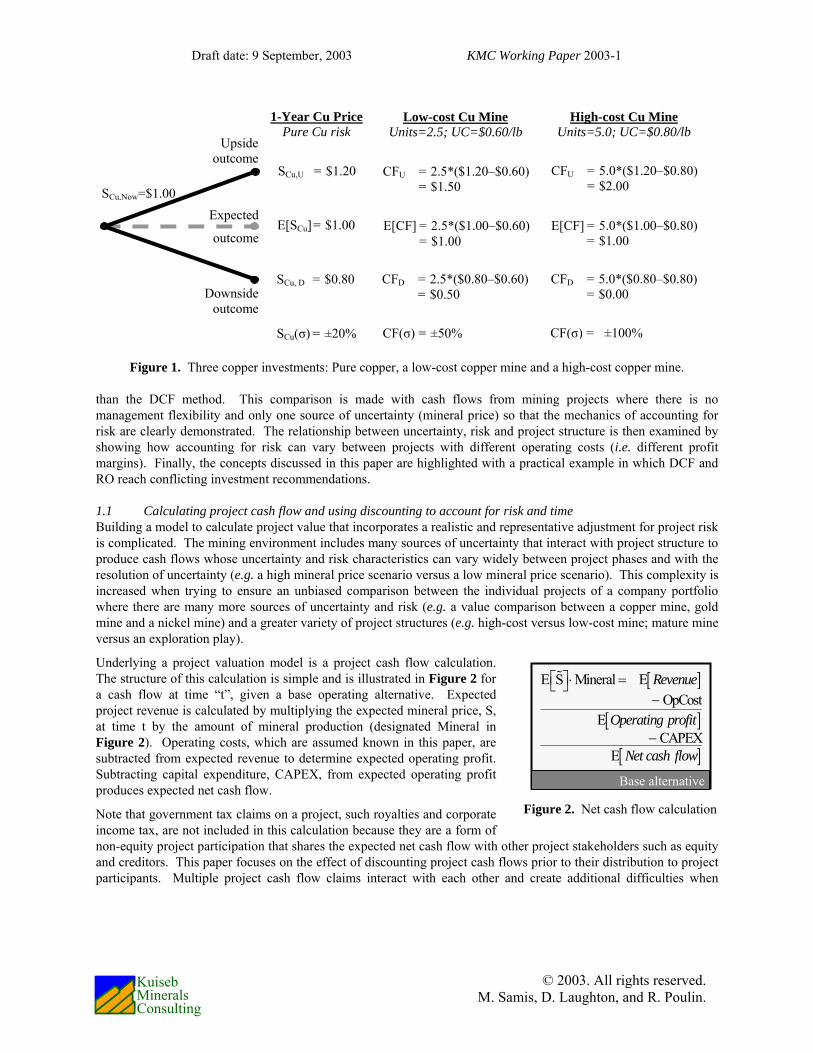
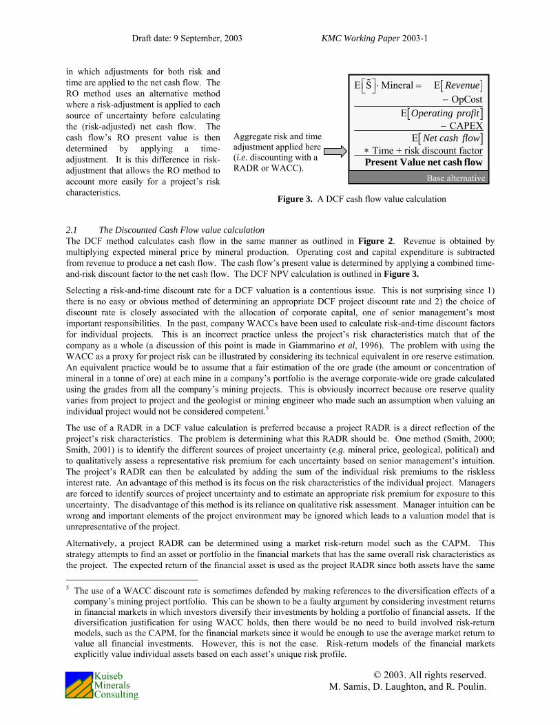
To illustrate the value effect of uncertainty, consider the three possible one year copper investments presented Figure 1. The current copper price is $1.00/lb and its expected price in one year is also $1.00. Copper price uncertainty can be approximated by a binomial outcome where there is a 50% probability of an upside copper price of $1.20/lb and a 50% probability of a downside copper price of $0.80/lb. An investor buying pure copper to hold for a year is exposed to uncertainty of ±20%. An investor may also elect to invest in either a low-cost copper mine or a high-cost copper mine that both have one year of production remaining. The low-cost mine produces 2.5 lbs of copper at a known cost of $0.60/lb and the high-cost mine produces 5.0 lbs of copper at a known cost of $0.80/lb. Both mines have expected cash flows of $1.00 but cash flow uncertainty at the low-cost mine is ±50%, while at the high-cost mine, it is ±100%.

Each of these investments has the same source of uncertainty (the copper price) but different overall levels of uncertainty. The absolute levels of uncertainty in each of these investments is important because investors see less value in and will pay less for an investment with greater uncertainty and risk even when competing investments have the same expected cash flow. Thus, in this example, investors will value more highly a pound of copper to hold for a year than the high-cost mine’s $1.00 of cash flow since the investment uncertainty associated with the high-cost mine is much greater (100% versus 20%).

Determining adequate compensation for risk exposure is more complicated than accounting for the time value of money since this calculation is directly related to the project’s risk profile or characteristics. Two methods currently used by the mining industry to calculate project NPV that consider uncertainty, risk and the time value of money. These are the Discounted Cash Flow (DCF) and Real Option (RO) valuation methods of which the DCF method is more commonly used. This paper compares the two valuation methods based on their ability to account for risk. It demonstrates why the RO method is structurally better able to differentiate between projects based on risk profile

1 Industry commentators have remarked in the past about the low equity returns associated with the mining industry

and often explain them by citing difficult business conditions. An alternative explanation could be that these low returns are the result of unrecognized biases contained within current valuation methods.




Figure 1. Three copper investments: Pure copper, a low-cost copper mine and a high-cost copper mine.

than the DCF method. This comparison is made with cash flows from mining projects where there is no management flexibility and only one source of uncertainty (mineral price) so that the mechanics of accounting for risk are clearly demonstrated. The relationship between uncertainty, risk and project structure is then examined by showing how accounting for risk can vary between projects with different operating costs (i.e. different profit margins). Finally, the concepts discussed in this paper are highlighted with a practical example in which DCF and RO reach conflicting investment recommendations.

1.1 Calculating project cash flow and using discounting to account for risk and time Building a model to calculate project value that incorporates a realistic and representative adjustment for project risk is complicated. The mining environment includes many sources of uncertainty that interact with project structure to produce cash flows whose uncertainty and risk characteristics can vary widely between project phases and with the resolution of uncertainty (e.g. a high mineral price scenario versus a low mineral price scenario). This complexity is increased when trying to ensure an unbiased comparison between the individual projects of a company portfolio where there are many more sources of uncertainty and risk (e.g. a value comparison between a copper mine, gold mine and a nickel mine) and a greater variety of project structures (e.g. high-cost versus low-cost mine; mature mine versus an exploration play).

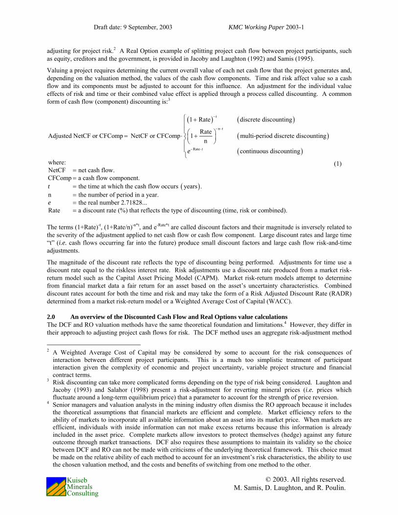
Underlying a project valuation model is a project cash flow calculation. The structure of this calculation is simple and is illustrated in Figure 2 for a cash flow at time “t”, given a base operating alternative. Expected project revenue is calculated by multiplying the expected mineral price, S, at time t by the amount of mineral production (designated Mineral in Figure 2). Operating costs, which are assumed known in this paper, are subtracted from expected revenue to determine expected operating profit. Subtracting capital expenditure, CAPEX, from expected operating profit produces expected net cash flow.

Note that government tax claims on a project, such royalties and corporate income tax, are not included in this calculation because they are a form of non-equity project participation that shares the expected net cash flow with other project stakeholders such as equity and creditors. This paper focuses on the effect of discounting project cash flows prior to their distribution to project participants. Multiple project cash flow claims interact with each other and create additional difficulties when

Figure 2. Net cash flow calculation

[ ]

[ ]

[ ]

E S Mineral EOpCost

ECAPEX

E

Revenue

Operating profit

Net cash flow

⎡ ⎤⋅ =⎣ ⎦−

−

Base alternative

Expected

outcome

SCu,Now=$1.00

Upside outcome

Downside outcome

1-Year Cu Price Pure Cu risk

SCu,U = $1.20

SCu, D = $0.80

SCu(σ) = ±20%

E[SCu] = $1.00

High-cost Cu Mine Units=5.0; UC=$0.80/lb

CFU = 5.0*($1.20–$0.80) = $2.00

E[CF] = 5.0*($1.00–$0.80)= $1.00

CF(σ) = ±100%

E[CF] = 2.5*($1.00–$0.60) = $1.00

CFD = 2.5*($0.80–$0.60)= $0.50

CF(σ) = ±50%

Low-cost Cu Mine Units=2.5; UC=$0.60/lb

CFU = 2.5*($1.20–$0.60) = $1.50

CFD = 5.0*($0.80–$0.80) = $0.00




adjusting for project risk.2 A Real Option example of splitting project cash flow between project participants, such as equity, creditors and the government, is provided in Jacoby and Laughton (1992) and Samis (1995).

Valuing a project requires determining the current overall value of each net cash flow that the project generates and, depending on the valuation method, the values of the cash flow components. Time and risk affect value so a cash flow and its components must be adjusted to account for this influence. An adjustment for the individual value effects of risk and time or their combined value effect is applied through a process called discounting. A common form of cash flow (component) discounting is:3

( ) ( )

( )

( )

n

Rate

1 Rate discrete discounting

RateAdjusted NetCF or CFComp NetCF or CFComp 1 multi-period discrete discountingn

continuous discounting

where:NetCF net cash flow.CFComp a cash flow

t

t

te

−

− ⋅

− ⋅

⎧ +⎪⎪⎛ ⎞= ⋅ +⎨⎜ ⎟⎝ ⎠⎪⎪⎩

==

( ) component.

the time at which the cash flow occurs years .n the number of period in a year.

the real number 2.71828... Rate a discount rate (%) that reflects the type of discounting (time, risk or co

t

e

==== mbined).

(1)

The terms (1+Rate)-t, (1+Rate/n)-n*t, and e-Rate*t are called discount factors and their magnitude is inversely related to the severity of the adjustment applied to net cash flow or cash flow component. Large discount rates and large time “t” (i.e. cash flows occurring far into the future) produce small discount factors and large cash flow risk-and-time adjustments.

The magnitude of the discount rate reflects the type of discounting being performed. Adjustments for time use a discount rate equal to the riskless interest rate. Risk adjustments use a discount rate produced from a market risk-return model such as the Capital Asset Pricing Model (CAPM). Market risk-return models attempt to determine from financial market data a fair return for an asset based on the asset’s uncertainty characteristics. Combined discount rates account for both the time and risk and may take the form of a Risk Adjusted Discount Rate (RADR) determined from a market risk-return model or a Weighted Average Cost of Capital (WACC).

2.0 An overview of the Discounted Cash Flow and Real Options value calculations The DCF and RO valuation methods have the same theoretical foundation and limitations.4 However, they differ in their approach to adjusting project cash flows for risk. The DCF method uses an aggregate risk-adjustment method

2 A Weighted Average Cost of Capital may be considered by some to account for the risk consequences of

interaction between different project participants. This is a much too simplistic treatment of participant interaction given the complexity of economic and project uncertainty, variable project structure and financial contract terms.

3 Risk discounting can take more complicated forms depending on the type of risk being considered. Laughton and Jacoby (1993) and Salahor (1998) present a risk-adjustment for reverting mineral prices (i.e. prices which fluctuate around a long-term equilibrium price) that a parameter to account for the strength of price reversion.

4 Senior managers and valuation analysts in the mining industry often dismiss the RO approach because it includes the theoretical assumptions that financial markets are efficient and complete. Market efficiency refers to the ability of markets to incorporate all available information about an asset into its market price. When markets are efficient, individuals with inside information can not make excess returns because this information is already included in the asset price. Complete markets allow investors to protect themselves (hedge) against any future outcome through market transactions. DCF also requires these assumptions to maintain its validity so the choice between DCF and RO can not be made with criticisms of the underlying theoretical framework. This choice must be made on the relative ability of each method to account for an investment’s risk characteristics, the ability to use the chosen valuation method, and the costs and benefits of switching from one method to the other.




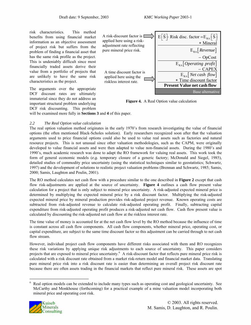
in which adjustments for both risk and time are applied to the net cash flow. The RO method uses an alternative method where a risk-adjustment is applied to each source of uncertainty before calculating the (risk-adjusted) net cash flow. The cash flow’s RO present value is then determined by applying a time-adjustment. It is this difference in risk-adjustment that allows the RO method to account more easily for a project’s risk characteristics.

2.1 The Discounted Cash Flow value calculation The DCF method calculates cash flow in the same manner as outlined in Figure 2. Revenue is obtained by multiplying expected mineral price by mineral production. Operating cost and capital expenditure is subtracted from revenue to produce a net cash flow. The cash flow’s present value is determined by applying a combined time- and-risk discount factor to the net cash flow. The DCF NPV calculation is outlined in Figure 3.

Selecting a risk-and-time discount rate for a DCF valuation is a contentious issue. This is not surprising since 1) there is no easy or obvious method of determining an appropriate DCF project discount rate and 2) the choice of discount rate is closely associated with the allocation of corporate capital, one of senior management’s most important responsibilities. In the past, company WACCs have been used to calculate risk-and-time discount factors for individual projects. This is an incorrect practice unless the project’s risk characteristics match that of the company as a whole (a discussion of this point is made in Giammarino et al, 1996). The problem with using the WACC as a proxy for project risk can be illustrated by considering its technical equivalent in ore reserve estimation. An equivalent practice would be to assume that a fair estimation of the ore grade (the amount or concentration of mineral in a tonne of ore) at each mine in a company’s portfolio is the average corporate-wide ore grade calculated using the grades from all the company’s mining projects. This is obviously incorrect because ore reserve quality varies from project to project and the geologist or mining engineer who made such an assumption when valuing an individual project would not be considered competent.5

The use of a RADR in a DCF value calculation is preferred because a project RADR is a direct reflection of the project’s risk characteristics. The problem is determining what this RADR should be. One method (Smith, 2000; Smith, 2001) is to identify the different sources of project uncertainty (e.g. mineral price, geological, political) and to qualitatively assess a representative risk premium for each uncertainty based on senior management’s intuition. The project’s RADR can then be calculated by adding the sum of the individual risk premiums to the riskless interest rate. An advantage of this method is its focus on the risk characteristics of the individual project. Managers are forced to identify sources of project uncertainty and to estimate an appropriate risk premium for exposure to this uncertainty. The disadvantage of this method is its reliance on qualitative risk assessment. Manager intuition can be wrong and important elements of the project environment may be ignored which leads to a valuation model that is unrepresentative of the project.

Alternatively, a project RADR can be determined using a market risk-return model such as the CAPM. This strategy attempts to find an asset or portfolio in the financial markets that has the same overall risk characteristics as the project. The expected return of the financial asset is used as the project RADR since both assets have the same 5 The use of a WACC discount rate is sometimes defended by making references to the diversification effects of a

company’s mining project portfolio. This can be shown to be a faulty argument by considering investment returns in financial markets in which investors diversify their investments by holding a portfolio of financial assets. If the diversification justification for using WACC holds, then there would be no need to build involved risk-return models, such as the CAPM, for the financial markets since it would be enough to use the average market return to value all financial investments. However, this is not the case. Risk-return models of the financial markets explicitly value individual assets based on each asset’s unique risk profile.

[ ]

[ ]

[ ]

E S Mineral E OpCost

E CAPEX

ETime + risk discount factor

Revenue

Operating profit

Net cash flow

⎡ ⎤ ⋅ =⎣ ⎦−

−

∗Present Value net cash flow

Base alternative

Aggregate risk and time adjustment applied here (i.e. discounting with a RADR or WACC).

Figure 3. A DCF cash flow value calculation




risk characteristics. This method benefits from using financial market information as an objective assessment of project risk but suffers from the problem of finding a financial asset that has the same risk profile as the project. This is undeniably difficult since most financially traded assets derive their value from a portfolio of projects that are unlikely to have the same risk characteristics as the project.

The arguments over the appropriate DCF discount rates are ultimately immaterial since they do not address an important structural problem underlying DCF risk discounting. This problem will be examined more fully in Sections 3 and 4 of this paper.

2.2 The Real Option value calculation The real option valuation method originates in the early 1970’s from research investigating the value of financial options (the often mentioned Black-Scholes solution). Early researchers recognized soon after that the valuation arguments used to price financial options could also be used to value real assets such as factories and natural resource projects. This is not unusual since other valuation methodologies, such as the CAPM, were originally developed to value financial assets and were then adapted to value non-financial assets. During the 1980’s and 1990’s, much academic research was done to adapt the RO framework for valuing real assets. This work took the form of general economic models (e.g. temporary closure of a generic factory; McDonald and Siegel, 1985), detailed studies of commodity price uncertainty (using the statistical techniques similar to geostatistics; Schwartz, 1997) and the development of solutions to realistic project valuation problems (Brennan and Schwartz, 1985; Samis, 2000; Samis, Laughton and Poulin, 2001).

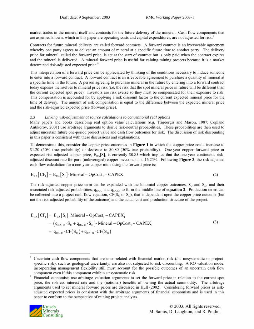
The RO method calculates net cash flow with a procedure similar to the one described in Figure 2 except that cash flow risk-adjustments are applied at the source of uncertainty. Figure 4 outlines a cash flow present value calculation for a project that is only subject to mineral price uncertainty. A risk-adjusted expected mineral price is determined by multiplying the expected mineral price by a risk discount factor. Multiplying the risk-adjusted expected mineral price by mineral production provides risk-adjusted project revenue. Known operating costs are subtracted from risk-adjusted revenue to calculate risk-adjusted operating profit. Finally, subtracting capital expenditure from risk-adjusted operating profit produces a risk-adjusted net cash flow. Cash flow present value is calculated by discounting the risk-adjusted net cash flow at the riskless interest rate.

The time value of money is accounted for at the net cash flow level by the RO method because the influence of time is constant across all cash flow components. All cash flow components, whether mineral price, operating cost, or capital expenditure, are subject to the same time discount factor so this adjustment can be carried through to net cash flow stream.

However, individual project cash flow components have different risks associated with them and RO recognizes these risk variations by applying unique risk adjustments to each source of uncertainty. This paper considers projects that are exposed to mineral price uncertainty.6 A risk-discount factor that reflects pure mineral price risk is calculated with a risk discount rate obtained from a market risk-return model and financial market data. Translating pure mineral price risk into a risk discount rate is easier than determining an overall project risk discount rate because there are often assets trading in the financial markets that reflect pure mineral risk. These assets are spot

6 Real option models can be extended to include many types such as operating cost and geological uncertainty. See

McCarthy and Monkhouse (forthcoming) for a practical example of a mine valuation model incorporating both mineral price and operating cost risk.

A risk-discount factor is applied here using a risk-adjustment rate reflecting pure mineral price risk.

A time discount factor is applied here using the riskless interest rate.

[ ]

[ ]

[ ]

RA

RA

RA

RA

E S Risk disc. factor E S Mineral

E OpCost

E CAPEX

E Time discount factor

Revenue

Operating profit

Net cash flow

⎡ ⎤ ⎡ ⎤⋅ =⎣ ⎦ ⎣ ⎦∗

−

−

∗Present Value net cash flow

Base alternative

Figure 4. A Real Option value calculation




market trades in the mineral itself and contracts for the future delivery of the mineral. Cash flow components that are assumed known, which in this paper are operating costs and capital expenditures, are not adjusted for risk.7

Contracts for future mineral delivery are called forward contracts. A forward contract is an irrevocable agreement whereby one party agrees to deliver an amount of mineral at a specific future time to another party. The delivery price for mineral, called the forward price, is set at the start of contract but is only paid when the contract expires and the mineral is delivered. A mineral forward price is useful for valuing mining projects because it is a market determined risk-adjusted expected price.8

This interpretation of a forward price can be appreciated by thinking of the conditions necessary to induce someone to enter into a forward contract. A forward contract is an irrevocable agreement to purchase a quantity of mineral at a specific time in the future. A person agreeing to purchase mineral in the future by entering into a forward contract today exposes themselves to mineral price risk (i.e. the risk that the spot mineral price in future will be different than the current expected spot price). Investors are risk averse so they must be compensated for their exposure to risk. This compensation is accounted for by applying a risk discount factor to the current expected mineral price for the time of delivery. The amount of risk compensation is equal to the difference between the expected mineral price and the risk-adjusted expected price (forward price).

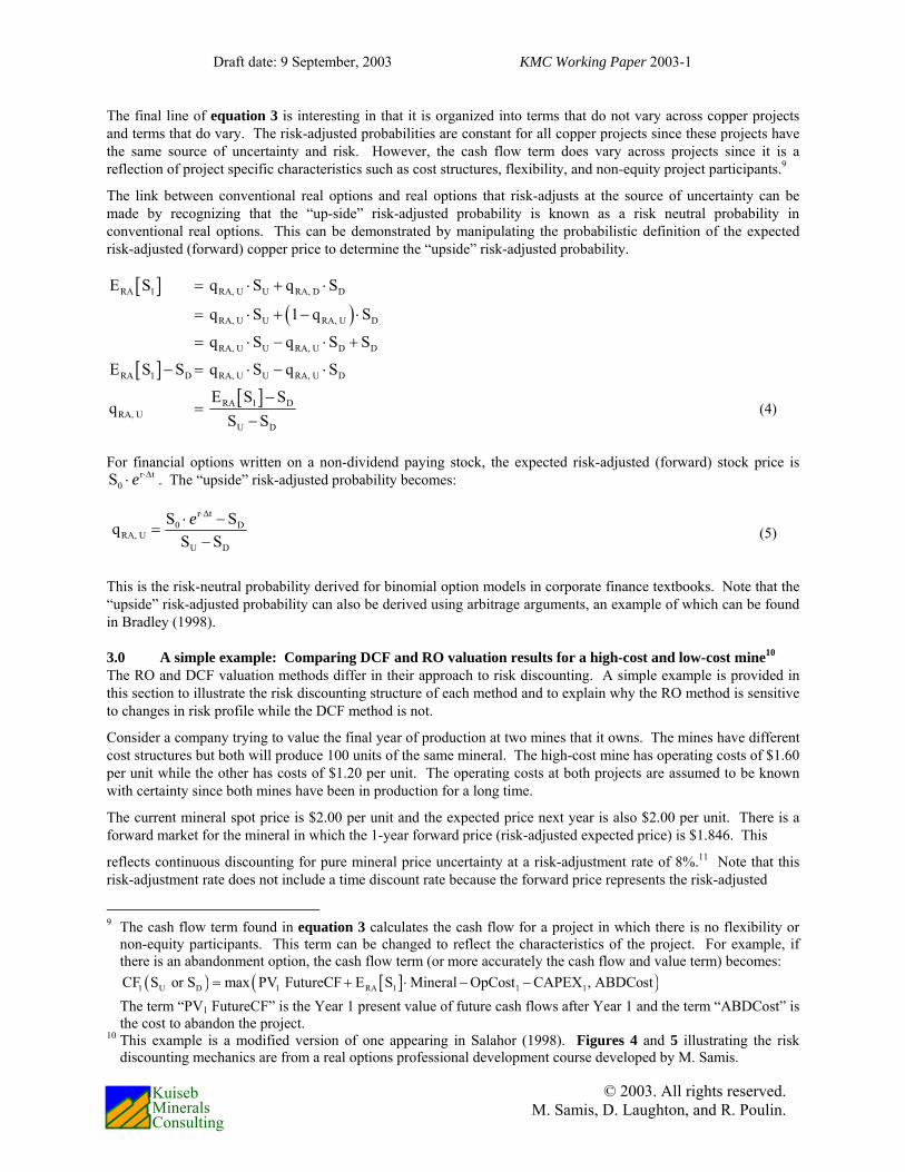
2.3 Linking risk-adjustment at source calculations to conventional real options Many papers and books describing real option value calculations (e.g. Trigeorgis and Mason, 1987; Copland Antikorov, 2001) use arbitrage arguments to derive risk-neutral probabilities. These probabilities are then used to adjust uncertain future one-period project value and cash flow outcomes for risk. The discussion of risk discounting in this paper is consistent with these discussions and explanations.

To demonstrate this, consider the copper price outcomes in Figure 1 in which the copper price could increase to $1.20 (50% true probability) or decrease to $0.80 (50% true probability). One-year copper forward price or expected risk-adjusted copper price, ERA[S], is currently $0.85 which implies that the one-year continuous risk-adjusted discount rate for pure (unleveraged) copper investments is 16.25%. Following Figure 2, the risk-adjusted cash flow calculation for a one-year copper mine using the forward price is:

[ ] [ ]RA 1 RA 1 1 1E CF E S Mineral OpCost CAPEX= ⋅ − − (2)

The risk-adjusted copper price term can be expanded with the binomial copper outcomes, SU and SD, and their associated risk-adjusted probabilities, qRA,U and qRA,D, to form the middle line of equation 3. Production terms can be collected into a project cash flow equation, CF(SU or SD), that is dependent upon the copper price outcome (but not the risk-adjusted probability of the outcome) and the actual cost and production structure of the project.

(3)

7 Uncertain cash flow components that are uncorrelated with financial market risk (i.e. unsystematic or project-

specific risk), such as geological uncertainty, are also not subjected to risk discounting. A RO valuation model incorporating management flexibility still must account for the possible outcomes of an uncertain cash flow component even if this component exhibits unsystematic risk.

8 Financial economists use arbitrage valuation arguments to set the forward price in relation to the current spot price, the riskless interest rate and the (notional) benefits of owning the actual commodity. The arbitrage arguments used to set mineral forward prices are discussed in Hull (2002). Considering forward prices as risk-adjusted expected prices is consistent with the arbitrage arguments of financial economists and is used in this paper to conform to the perspective of mining project analysts.

[ ] [ ]( )

( ) ( )

RA 1 RA 1 1 1

RA, U U RA, D D 1 1

RA, U U RA, D D

E CF E S Mineral OpCost CAPEX

q S q S Mineral OpCost CAPEX

q CF S q CF S

= ⋅ − −

= ⋅ + ⋅ ⋅ − −

= ⋅ + ⋅




The final line of equation 3 is interesting in that it is organized into terms that do not vary across copper projects and terms that do vary. The risk-adjusted probabilities are constant for all copper projects since these projects have the same source of uncertainty and risk. However, the cash flow term does vary across projects since it is a reflection of project specific characteristics such as cost structures, flexibility, and non-equity project participants.9

The link between conventional real options and real options that risk-adjusts at the source of uncertainty can be made by recognizing that the “up-side” risk-adjusted probability is known as a risk neutral probability in conventional real options. This can be demonstrated by manipulating the probabilistic definition of the expected risk-adjusted (forward) copper price to determine the “upside” risk-adjusted probability.

(4)

For financial options written on a non-dividend paying stock, the expected risk-adjusted (forward) stock price is r t

0S e ⋅∆⋅ . The “upside” risk-adjusted probability becomes:

(5)

This is the risk-neutral probability derived for binomial option models in corporate finance textbooks. Note that the “upside” risk-adjusted probability can also be derived using arbitrage arguments, an example of which can be found in Bradley (1998).

3.0 A simple example: Comparing DCF and RO valuation results for a high-cost and low-cost mine10 The RO and DCF valuation methods differ in their approach to risk discounting. A simple example is provided in this section to illustrate the risk discounting structure of each method and to explain why the RO method is sensitive to changes in risk profile while the DCF method is not.

Consider a company trying to value the final year of production at two mines that it owns. The mines have different cost structures but both will produce 100 units of the same mineral. The high-cost mine has operating costs of $1.60 per unit while the other has costs of $1.20 per unit. The operating costs at both projects are assumed to be known with certainty since both mines have been in production for a long time.

The current mineral spot price is $2.00 per unit and the expected price next year is also $2.00 per unit. There is a forward market for the mineral in which the 1-year forward price (risk-adjusted expected price) is $1.846. This

reflects continuous discounting for pure mineral price uncertainty at a risk-adjustment rate of 8%.11 Note that this risk-adjustment rate does not include a time discount rate because the forward price represents the risk-adjusted

9 The cash flow term found in equation 3 calculates the cash flow for a project in which there is no flexibility or

non-equity participants. This term can be changed to reflect the characteristics of the project. For example, if there is an abandonment option, the cash flow term (or more accurately the cash flow and value term) becomes:

( ) [ ]( )1 U D 1 RA 1 1 1CF S or S max PV FutureCF E S Mineral OpCost CAPEX , ABDCost= + ⋅ − − The term “PV1 FutureCF” is the Year 1 present value of future cash flows after Year 1 and the term “ABDCost” is

the cost to abandon the project. 10 This example is a modified version of one appearing in Salahor (1998). Figures 4 and 5 illustrating the risk

discounting mechanics are from a real options professional development course developed by M. Samis.

[ ]( )

[ ][ ]

RA 1 RA, U U RA, D D

RA, U U RA, U D

RA, U U RA, U D D

RA 1 D RA, U U RA, U D

RA 1 DRA, U

U D

E S q S q S

q S 1 q S

q S q S S

E S S q S q S

E S Sq

S S

= ⋅ + ⋅

= ⋅ + − ⋅

= ⋅ − ⋅ +

− = ⋅ − ⋅

−=

−

r t0 D

RA, UU D

S SqS S

e ⋅∆⋅ −=

−




Table 1. Analysis of cash flow risk and time discounting

value of mineral delivered in one year. The current riskless interest rate obtained from the government bond market is 5%. The company currently has a policy of using a DCF RADR of 15% in all its project valuations which combines a 10% adjustment for risk and the time value of money.

Table 1 outlines the value calculation and provides a breakdown of cash flow discounting for both DCF and RO. Section 1 of the table outlines the calculation of expected net cash flow. Both projects have expected revenue of $200. However, the high-cost project has a net cash flow of $40 and the low-cost project has a net cash flow of $80 due to differences in operating cost.

If the DCF method is used, project NPVs would be calculated by multiplying the net cash flow of each project by a risk-and-time discount factor of 0.8607 (from an RADR of 15%). DCF NPV of the high-cost project is $34.43 and $68.86 for the low-cost project.

The RO risk-adjustment calculation is outlined in the Section 2 of the table. A risk-adjustment for mineral price uncertainty is factored into the revenue calculation by multiplying the risk-adjusted expected mineral (forward) price of $1.8462 by mineral production. This represents a risk discount rate of 8% for pure mineral uncertainty. Note that risk-adjusted revenue is the same for both projects since both produce the same amount of mineral. Costs are not adjusted for risk because they are assumed known. A risk-adjusted net cash flow is produced by subtracting operating costs from revenue. The high-cost project has a risk-adjusted net cash flow of $24.62 and the low-cost project a risk-adjusted net cash flow of $64.62.

11 Developing models of mineral spot and forward prices is not trivial since the relationship between a commodity

and other financial assets can be complex and the financial market data necessary to estimate model parameters are incomplete. A very simple model is used in this example for demonstration purposes only.

Time value of money Project 1 Project 2Risk-free discount factor 0.9512 Section 1: Expected cash flowRisk-free discount rate 5.00% Production 100.00 100.00

Revenue $200.00 $200.00Mineral price model Cost $160.00 $120.00Current Year 1 expected price 2.0000 Net cash flow $40.00 $80.00Risk discount factor 0.9231 Section 2: Risk-adjusted cash flowRisk discount rate 8.00% Revenue $184.62 $184.62Mineral forward price ( $/unit ) 1.8462 Cost $160.00 $120.00

Net $24.62 $64.62DCF valuation results Section 3: Time- and risk-adjusted cash flowRADR (%) 15.0% Revenue $175.62 $175.62Project 1 $34.43 Cost $152.20 $114.15Difference between RO and DCF $11.01 Net $23.42 $61.47Project 2 $68.86 Section 4: Continuous discount ratesDifference between RO and DCF $7.39 Effective risk discount rate

Revenue 8.00% 8.00%Cost 0.00% 0.00%Net cash flow 48.52% 21.35%Effective risk and time discount rateRevenue 13.00% 13.00%Cost 5.00% 5.00%Net cash flow 53.52% 26.35%




An adjustment for time is applied in the third section of the table. Each cash flow stream in the RO calculation is multiplied by a time discounted factor of 0.9512, derived from a risk-free discount rate of 5%, to reach a present value of $23.42 for the high-cost project and $61.47 for the low-cost project.

The final two sections of Table 1 present the effective discount rates applied to each cash flow stream by the real options method. These rates are determined by comparing the expected cash flow stream magnitude in the first section of the table to that of the second or third section and then back-calculating the required discount rate using the continuous discounting formula. The equation (using a natural logarithm) to determine the effective discount rate in Section 4 is:

Adjusted CF stream (from table or )Discount rate lnUnadjusted CF stream (from table )

⎛ ⎞= − ⎜ ⎟

⎝ ⎠

section 2 3section 1

(6)

The effective risk discount rate applied to the revenue streams of both projects is 8%. This is expected since both projects produce the same mineral and are exposed to the same mineral price risk. The cost streams of both projects attract no effective risk adjustment because operating costs are considered known. The biggest discounting effect is found in the net cash flow stream where the effective risk discount is 48.5% for the high-cost project and 21.4% for the low-cost project. Adding in a time adjustment produces an overall effective risk-adjusted discount rate of 53.5% for the high-cost project and 26.4% for the low-cost project. The difference in discounting at the net cash flow level is also reasonable given that cash flows from the high-cost project are much more sensitive to changes in the operating costs from revenue. The high-cost project has a risk-adjusted net cash flow of $24.62 and the low-cost project a risk-adjusted net cash flow of $64.62.

The effective risk discount rate applied to the revenue streams of both projects is 8%. This is expected since both projects produce the same mineral and are exposed to the same mineral price risk. The cost streams of both projects attract no effective risk adjustment because operating costs are considered known. The biggest discounting effect is found in the net cash flow stream where the effective risk discount is 48.5% for the high-cost project and 21.4% for the low-cost project. Adding in a time adjustment produces an overall effective risk-adjusted discount rate of 53.5% for the high-cost project and 26.4% for the low-cost project. The difference in discounting at the net cash flow level is also reasonable given that cash flows from the high-cost project are much more sensitive to changes in the underlying mineral price than those from the low-cost project. That both projects attract higher effective discount rates with RO suggests that the DCF RADR of 15% incorporates a risk adjustment that is too small.

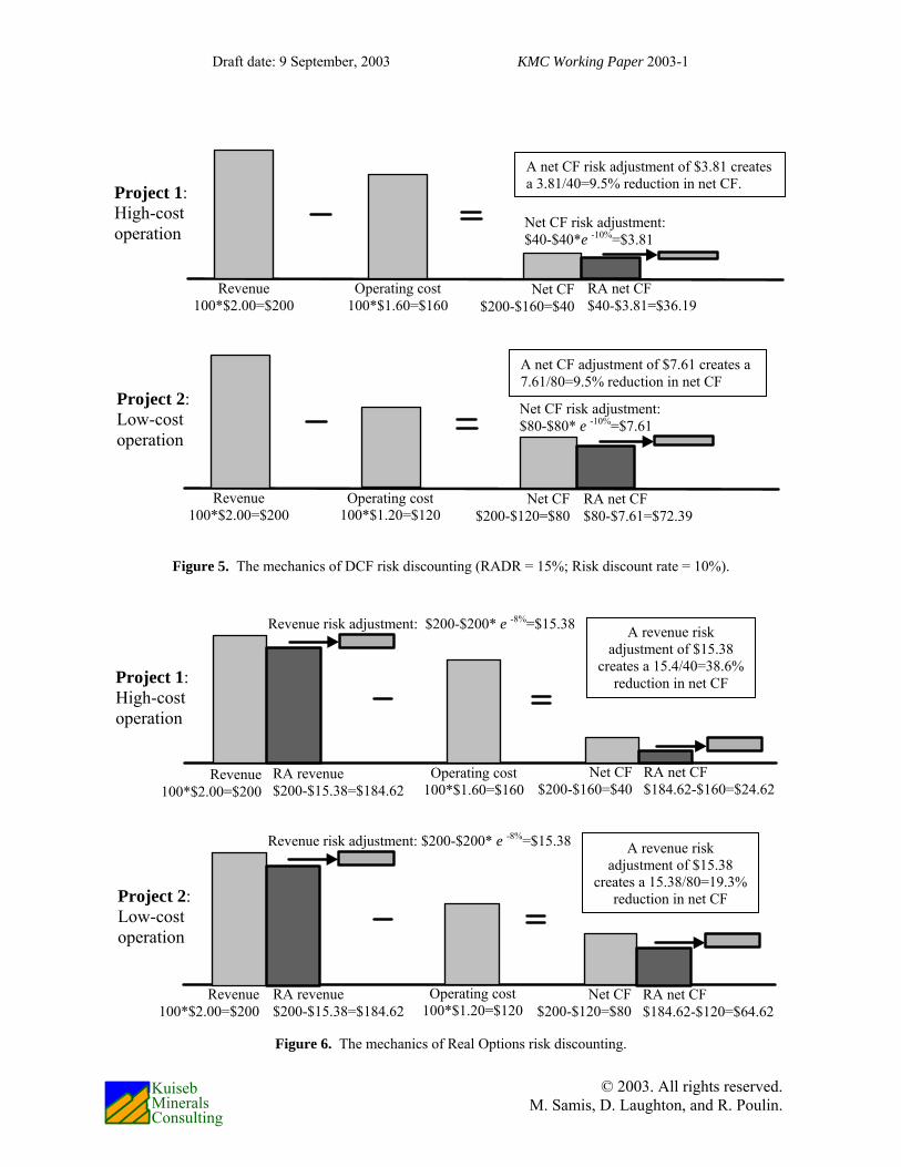
The mechanics of the DCF risk adjustment is illustrated in Figure 5. Revenue of $200 is produced by both projects and is represented by the left-most bar with light-colored infilling. Net cash flow from each project is calculated by subtracting operating cash flow from revenue. Net cash flow is represented by the lightly colored in-filled bar on the right side. The magnitude of net cash flow without a risk-adjustment is indicated by the height of each net cash flow bar.

A 10% risk discount rate is used for the DCF calculations in Figure 5 because this figure is focused on the risk-adjustment mechanics of DCF and this is the risk-adjustment portion of the 15% RADR (i.e. 15% less the riskless interest rate of 5%). The 5% time discount rate is ignored because it can not highlight the discounting differences between DCF and RO given this rate affects all cash flow streams equally. The cross-hatched bars on the right-hand side of Figure 5 represent the risk-adjusted net cash flows from each project. The magnitude of the risk-adjustment is indicated by the solid-colored slice on the right-hand side and is equal to the difference between the net cash flow and risk-adjusted net cash flow.

It is interesting to look at the absolute and relative effects of the DCF risk adjustment. A risk discount rate of 10% produces a net risk adjustment of $3.81 for the high-cost project and $7.61 for the low-cost project. The absolute magnitude of risk-adjustment is larger for the low-cost project because the 10% risk-adjustment rate is being applied to a larger net cash flow. However, on a relative basis, each risk-adjustment represents a 9.5% reduction in net cash flow regardless of the project cost structure. This demonstrates that the DCF method effectively applies the same risk discount to each $1 of net cash flow regardless of project cost structure.




Figure 5. The mechanics of DCF risk discounting (RADR = 15%; Risk discount rate = 10%).

Figure 6. The mechanics of Real Options risk discounting.

Project 1: High-cost operation

Project 2: Low-cost operation

Revenue 100*$2.00=$200

Operating cost 100*$1.60=$160

Net CF$200-$160=$40

RA net CF $40-$3.81=$36.19

Net CF risk adjustment: $40-$40*e -10%=$3.81

A net CF risk adjustment of $3.81 creates a 3.81/40=9.5% reduction in net CF.

Revenue 100*$2.00=$200


Net CF$200-$120=$80

RA net CF $80-$7.61=$72.39

Net CF risk adjustment: $80-$80* e -10%=$7.61

A net CF adjustment of $7.61 creates a 7.61/80=9.5% reduction in net CF

Revenue risk adjustment: $200-$200* e -8%=$15.38

Project 1: High-cost operation

Project 2: Low-cost operation

Revenue risk adjustment: $200-$200* e -8%=$15.38


RA revenue $200-$15.38=$184.62

Revenue 100*$2.00=$200

Net CF $200-$160=$40

RA net CF $184.62-$160=$24.62

A revenue risk adjustment of $15.38

creates a 15.4/40=38.6% reduction in net CF

Revenue 100*$2.00=$200

RA revenue $200-$15.38=$184.62


Net CF$200-$120=$80

RA net CF $184.62-$120=$64.62

A revenue risk adjustment of $15.38

creates a 15.38/80=19.3% reduction in net CF




The risk-adjustment mechanics of real options is presented in Figure 6. Once again, the lightly-colored in-filled bars represent the unadjusted revenue, operating cost and net cash flow streams. In contrast to DCF, RO applies the risk-adjustment to the revenue stream through the use of the risk-adjusted expected mineral price of $1.8462. Both projects have risk-adjusted revenue of $184.62, represented by the cross-hatched bars on the left, since they produce equal amounts of the same mineral. The absolute magnitude of the revenue risk adjustment is $15.38 which is represented by the solid colored slice on the left. Risk-adjusted net cash flow is calculated by subtracting known operating costs from the risk-adjusted revenue. The risk-adjusted net cash flow is $24.62 for the high-cost project and $64.62 for the low-cost project.

What is interesting here is how the revenue risk-adjustment translates into a risk-adjustment to the net cash flow stream. For both projects, the absolute revenue risk-adjustment of $15.38 does not change in size when carried through to net cash flow stream. In other words, the net cash flow from both projects is reduced by the same absolute amount of $15.38. However, the impact of this risk-adjustment differs between projects when considered as a proportion of each project’s net cash flow. The revenue risk-adjustment represents a 38.4% reduction in net cash flow for the high-cost project and a 19.3% reduction for the low-cost project. These figures are calculated by subtracting the continuous discounting factor using the net cash flow risk-discount rates in Table 1 (48.5% and 21.4%) from 1 (i.e. 1 – e-0.485=0.384; 1-e-0.214=0.193).

Within RO valuation framework, each $1 of net cash flow from the high-cost project is worth only $0.614 on a risk-adjusted basis while each $1 of net cash flow from the low-cost project is worth $0.807. The difference in risk-adjusted value is entirely due to cost structure variations between the projects. High operating costs result in revenue risk adjustments having a larger impact on net cash flow than low operating costs.

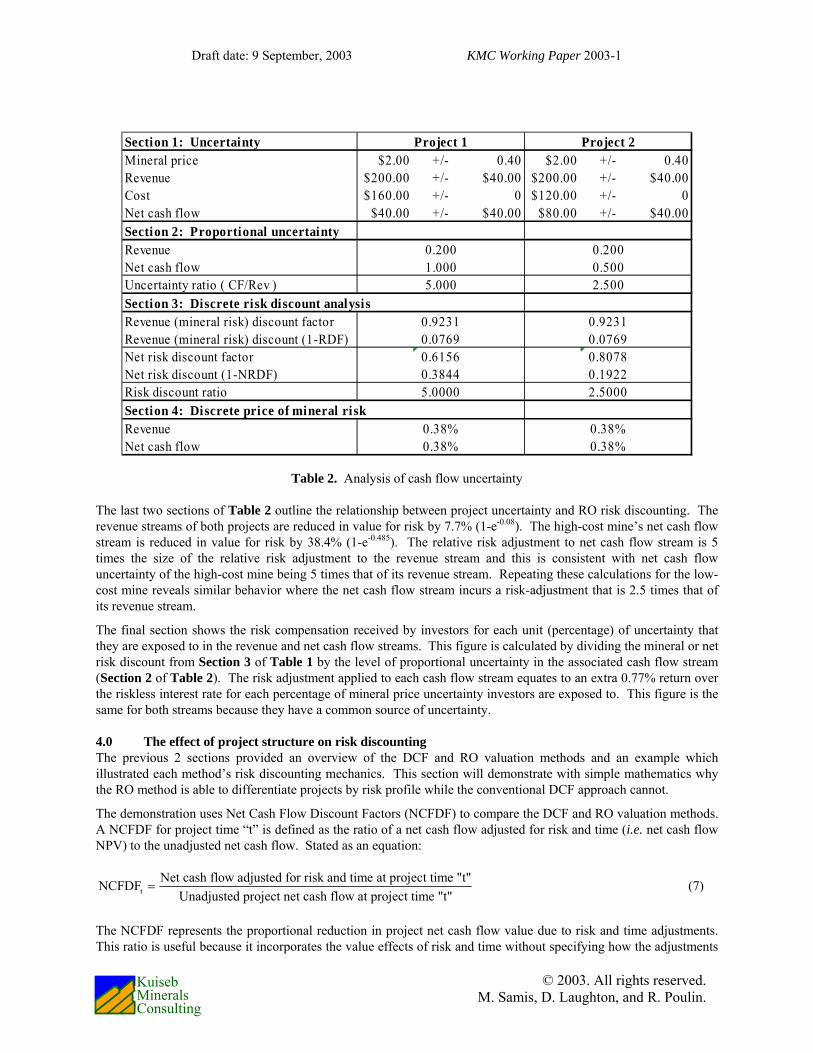
An important question that should be considered is whether it is acceptable for a high-cost project to be subject to larger risk adjustments than a low-cost project. It is widely accepted in the mining industry that cash flows from high-cost mines are more sensitive to mineral price variations than cash flows from low-cost projects so the use of larger risk-adjustments at higher-cost mines is not unreasonable.12 Table 2 demonstrates in more detail why the use of larger discount rates at high-cost mines makes sense and how mineral price uncertainty filters through the cost structure of each project.

Risk discounting is driven by cash flow uncertainty or the spread of possible cash flow values around a cash flow expectation. In this example, the mineral price is expected to be $2.00 in one year but may be 20% above or below this level giving mineral prices of either $1.60 or $2.40. This price uncertainty produces revenue uncertainty of 20% and results in $200 of expected revenue with possible revenue magnitudes of either $160 or $240 for both projects. Revenue uncertainty is magnified in the net cash flow stream by the known operating costs. The expected net cash flow from the high-cost project is $40.00 with possible net cash flows of either $0.00 or $80.00. The expected net cash flow from the low-cost project is $80.00 with possible net cash flows of either $40.00 or $120.00. In other words, net cash flow uncertainty is 100% for the high-cost project and 50% for the low-cost project.

This difference is important because a fundamental principle of valuation is that a risk-adjustment should be related directly to the level of cash flow uncertainty. Cash flows with greater magnitudes of uncertainty should in general attract risk adjustments that are larger than cash flows with lower levels of uncertainty due to investor risk aversion. In the second section of this table, net cash flow uncertainty in the high-cost project is 5 times the size of uncertainty in the revenue stream (net cash flow proportional uncertainty of 0.5 / revenue proportional uncertainty of 0.1) and twice the size of net cash flow uncertainty in the low-cost project.

The valuation policies and methods used to calculate value should recognize uncertainty variations between projects. In this example, the RO method directs a higher risk-adjustment to the high-cost mine net cash flow stream in response to this project’s higher levels of uncertainty while the use of a constant RADR of 15% within the DCF method ignores the difference in net cash flow uncertainty. At this point, it is easy to proclaim that all mining projects should be evaluated with RADRs linked to their risk profile. However, the author’s experience within the mining industry has been that many different projects are often valued with a constant RADR with a few exceptions possibly made for political risk.

12 Mining analysts often refer to high operating leverage as an explanation for the larger fluctuations in the equity

values of high-cost mines when compared to low-cost mines in response to significant mineral price changes.




Table 2. Analysis of cash flow uncertainty

The last two sections of Table 2 outline the relationship between project uncertainty and RO risk discounting. The revenue streams of both projects are reduced in value for risk by 7.7% (1-e-0.08). The high-cost mine’s net cash flow stream is reduced in value for risk by 38.4% (1-e-0.485). The relative risk adjustment to net cash flow stream is 5 times the size of the relative risk adjustment to the revenue stream and this is consistent with net cash flow uncertainty of the high-cost mine being 5 times that of its revenue stream. Repeating these calculations for the low-cost mine reveals similar behavior where the net cash flow stream incurs a risk-adjustment that is 2.5 times that of its revenue stream.

The final section shows the risk compensation received by investors for each unit (percentage) of uncertainty that they are exposed to in the revenue and net cash flow streams. This figure is calculated by dividing the mineral or net risk discount from Section 3 of Table 1 by the level of proportional uncertainty in the associated cash flow stream (Section 2 of Table 2). The risk adjustment applied to each cash flow stream equates to an extra 0.77% return over the riskless interest rate for each percentage of mineral price uncertainty investors are exposed to. This figure is the same for both streams because they have a common source of uncertainty.

4.0 The effect of project structure on risk discounting The previous 2 sections provided an overview of the DCF and RO valuation methods and an example which illustrated each method’s risk discounting mechanics. This section will demonstrate with simple mathematics why the RO method is able to differentiate projects by risk profile while the conventional DCF approach cannot.

The demonstration uses Net Cash Flow Discount Factors (NCFDF) to compare the DCF and RO valuation methods. A NCFDF for project time “t” is defined as the ratio of a net cash flow adjusted for risk and time (i.e. net cash flow NPV) to the unadjusted net cash flow. Stated as an equation:

tNet cash flow adjusted for risk and time at project time "t"NCFDF

Unadjusted project net cash flow at project time "t"= (7)

The NCFDF represents the proportional reduction in project net cash flow value due to risk and time adjustments. This ratio is useful because it incorporates the value effects of risk and time without specifying how the adjustments

Section 1: Uncertainty Project 1 Project 2Mineral price $2.00 +/- 0.40 $2.00 +/- 0.40Revenue $200.00 +/- $40.00 $200.00 +/- $40.00Cost $160.00 +/- 0 $120.00 +/- 0Net cash flow $40.00 +/- $40.00 $80.00 +/- $40.00Section 2: Proportional uncertaintyRevenue 0.200 0.200Net cash flow 1.000 0.500Uncertainty ratio ( CF/Rev ) 5.000 2.500Section 3: Discrete risk discount analysisRevenue (mineral risk) discount factor 0.9231 0.9231Revenue (mineral risk) discount (1-RDF) 0.0769 0.0769Net risk discount factor 0.6156 0.8078Net risk discount (1-NRDF) 0.3844 0.1922Risk discount ratio 5.0000 2.5000Section 4: Discrete price of mineral riskRevenue 0.38% 0.38%Net cash flow 0.38% 0.38%




for risk and time are made. The ratio becomes smaller as project risks become greater and the cash flow time horizon lengthens because there is an increase in the magnitude of adjustments for risk and time.

Net cash flow for the NCFDF is calculated as described in Figure 2 and is represented by the equation:

t 0

t

0

NetCF E S Mineral OpCost CAPEXwhere:NetCF net cash flow.E S the current expected mineral price.Mineral the amount of mineral produced.OpCost operating cost.CAPEX capital expenditure.

⎡ ⎤= ⋅ − −⎣ ⎦

=⎡ ⎤ =⎣ ⎦

===

(8)

This can be manipulated by dividing the operating costs by the amount of mineral produced so that:

( )t 0NetCF E S UnitOC Mineral CAPEXwhere:UnitOC unit operating cost OpCost Mineral

⎡ ⎤= − ⋅ −⎣ ⎦

= = (9)

As mentioned previously, the DCF uses an aggregate risk and time adjustment approach which produces a DCF NCFDF for a cash flow occurring at time “t”:

( )( )( )

0

DCF, t0

Risk rate t Time rate t

E S UnitOC Mineral CAPEXNCDF

E S UnitOC Mineral CAPEXwhere:RiskDF risk discount factor TimeDF time discount factore e− ⋅ − ⋅

⎡ ⎤ − ⋅ − ⋅ ⋅⎣ ⎦=⎡ ⎤ − ⋅ −⎣ ⎦

= = = =

DCFRiskDF TimeDF

(10)

This expression can be simplified by factoring out the net cash flow calculation so that, if continuous discounting is used:

Risk rate t Time rate t RADR tDCF, t DCFNCDF RiskDF TimeDF e e e− ⋅ − ⋅ − ⋅= ⋅ = ⋅ = (11)

Equation 11 shows that the DCF NCFDF is invariant to project structure. The DCF NCFDF of competing projects with different operating cost and capital expenditures will show no variation unless the RADR is changed to reflect differences in project risk. This is unlikely since it is valuation policy at many mining companies to use the same RADR for both high-cost and low-cost projects even though the cash flows from a high-cost project are more risky.

The RO method adjusts for risk at the uncertainty source and adjusts for time at the net cash flow stream which leads to a RO NCFDF:

( )( )( )

0

RO, t0

Mineral risk rate tRO

E S UnitOC Mineral CAPEXNCDF

E S UnitOC Mineral CAPEXwhere:RiskDF risk discount factor or a more complicated formula incorporating

the effects of e− ⋅

⎡ ⎤ ⋅ − ⋅ − ⋅⎣ ⎦=⎡ ⎤ − ⋅ −⎣ ⎦

= =

RORiskDF TimeDF

Time rate t

price reversion.TimeDF time discount factor e− ⋅= =

(12)




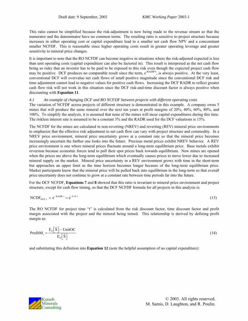
This ratio cannot be simplified because the risk-adjustment is now being made to the revenue stream so that the numerator and the denominator have no common terms. The resulting ratio is sensitive to project structure because increases in either operating cost or capital expenditure lead to a smaller net cash flow NPV and a concomitant smaller NCFDF. This is reasonable since higher operating costs result in greater operating leverage and greater sensitivity to mineral price changes. It is important to note that the RO NCFDF can become negative in situations where the risk-adjusted expected is less than unit operating costs (capital expenditure can also be factored in). This result is interpreted as the net cash flow being so risky that an investor has to be paid to be exposed to this risk even though the expected project cash flow may be positive. DCF produces no comparable result since the term, e-RADR*t, is always positive. At the very least, conventional DCF will overvalue net cash flows of small positive magnitude since the conventional DCF risk and time adjustment cannot lead to negative values for positive cash flows. Increasing the DCF RADR to reflect greater cash flow risk will not work in this situation since the DCF risk-and-time discount factor is always positive when discounting with Equation 11.

4.1 An example of changing DCF and RO NCFDF between projects with different operating costs The variation of NCFDF across projects of different structure is demonstrated in this example. A company owns 5 mines that will produce the same mineral over the next ten years at profit margins of 20%, 40%, 60%, 80%, and 100%. To simplify the analysis, it is assumed that none of the mines will incur capital expenditures during this time. The riskless interest rate is assumed to be a constant 3% and the RADR used for the DCF valuations is 15%.

The NCFDF for the mines are calculated in non-reverting (NREV) and reverting (REV) mineral price environments to emphasize that the effective risk adjustment to net cash flow can vary with project structure and commodity. In a NREV price environment, mineral price uncertainty grows at a constant rate so that the mineral price becomes increasingly uncertain the further one looks into the future. Precious metal prices exhibit NREV behavior. A REV price environment is one where mineral prices fluctuate around a long-term equilibrium price. Base metals exhibit reversion because economic forces tend to pull their spot prices back towards equilibrium. New mines are opened when the prices are above the long-term equilibrium which eventually causes prices to move lower due to increased mineral supply on the market. Mineral price uncertainty in a REV environment grows with time in the short-term but approaches an upper limit as the time horizon becomes longer because of the long-term equilibrium price. Market participants know that the mineral price will be pulled back into equilibrium in the long-term so that overall price uncertainty does not continue to grow at a constant rate between time periods far into the future.

For the DCF NCFDF, Equations 7 and 8 showed that this ratio is invariant to mineral price environment and project structure, except for cash flow timing, so that the DCF NCFDF formula for all projects in this analysis is:

RADR t 0.15 tDCF, tNCDF e e− ⋅ − ⋅= = (13)

The RO NCFDF for project time “t” is calculated from the risk discount factor, time discount factor and profit margin associated with the project and the mineral being mined. This relationship is derived by defining profit margin as:

0t

0

E S UnitOCProfitM

E S

⎡ ⎤ −⎣ ⎦=⎡ ⎤⎣ ⎦

(14)

and substituting this definition into Equation 12 (note the helpful assumption of no capital expenditure):




( )( )

( )( )( )( )

[ ] [ ]( )

0

RO, t

0

0 0

0 0

0 0 0

UnitOC E S ProfitM E S

E S RiskDF UnitOC Mineral TimeDFNCDF

E S UnitOC Mineral

E S RiskDF 1 ProfitM E S TimeDF

E S 1 ProfitM E S

E S RiskDF E S ProfitM E S

= − ⋅

⎡ ⎤ ⋅ − ⋅ ⋅⎣ ⎦=⎡ ⎤ − ⋅⎣ ⎦

⎡ ⎤ ⎡ ⎤⋅ − − ⋅ ⋅⎣ ⎦ ⎣ ⎦=⎡ ⎤ ⎡ ⎤− − ⋅⎣ ⎦ ⎣ ⎦

⎡ ⎤ ⎡ ⎤ ⎡ ⎤⋅ − + ⋅⎣ ⎦ ⎣ ⎦ ⎣=( )

( )( )

( )( )

0 0 0

0

0

RO, t

TimeDF

E S E S ProfitM E S

E S RiskDF 1 ProfitM TimeDF

E S 1 1 ProfitM

RiskDF ProfitM 1 TimeDFNCDF

ProfitM

⋅⎦⎡ ⎤ ⎡ ⎤ ⎡ ⎤− + ⋅⎣ ⎦ ⎣ ⎦ ⎣ ⎦

⎡ ⎤ ⋅ − + ⋅⎣ ⎦=⎡ ⎤ ⋅ − +⎣ ⎦

+ − ⋅=

(15)

The time discount factor in Equation 15 is determined from e-0.03*t. The profit margin is set either as 0.2, 0.4, 0.5, 0.8 or 1 since the unit operating costs can be set in relation to the expected mineral price to provide the needed profit margin. The risk discount factor is linked specifically to the market and uncertainty characteristics of the mineral being mined. If the mineral is non-reverting, this factor is calculated with the RO risk discount formula presented in Equation 12 with the mineral risk rate set to 6%. This mineral risk rate is based on the mineral price uncertainty (standard deviation=15%) and the price of mineral risk (0.4 or an extra 0.04% of return for each 1% of mineral price uncertainty). A more complicated formula is used to calculated the risk discount formula if the mineral price exhibits reversion.13 Note that mineral price uncertainty and the price of mineral risk is the same in both NREV and REV price environments.

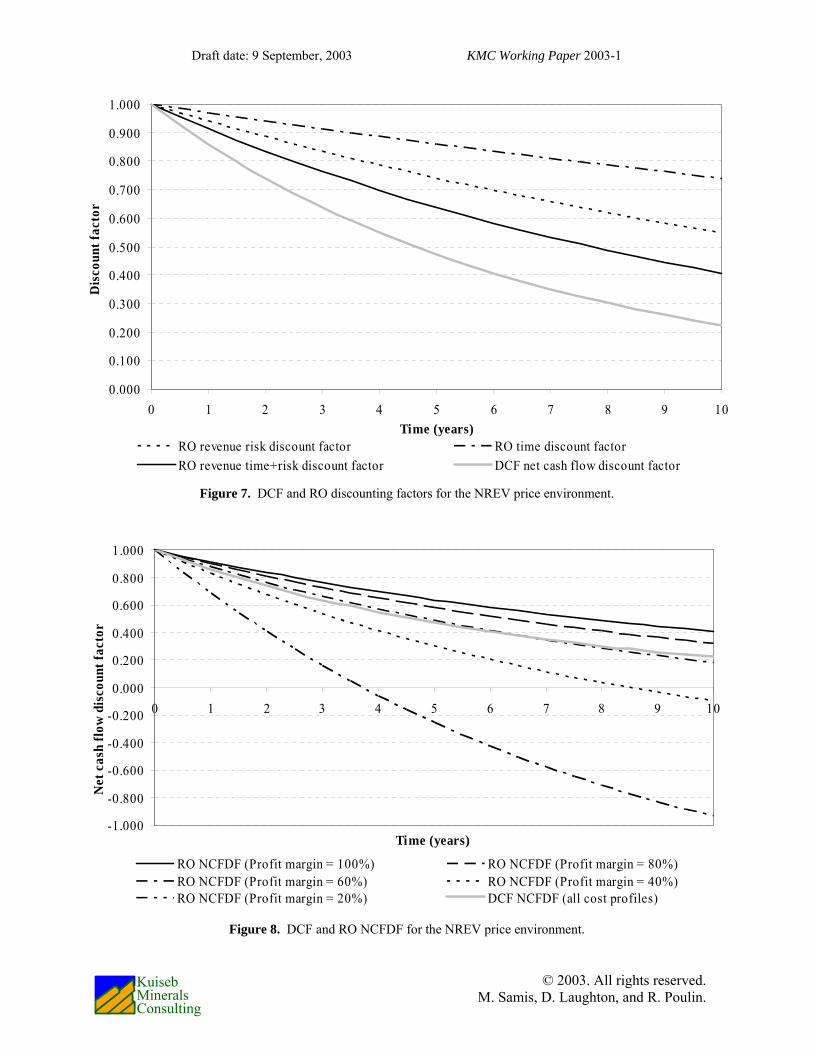
Figure 7 displays the risk and time discount factors for the NREV mineral price environment. The time discount factor is outlined by the upper line (dash-dot) in the graph. The mineral risk discount factor is represented by the dotted line immediately below the time discount factor. This factor decreases at a constant rate in a NREV price environment because mineral price uncertainty increases at a constant rate. The black solid line represents the RONCFDF for an asset exhibiting pure mineral price risk (e.g. a non-taxed 100% equity project with no operating costs and capital expenditures) and is produced by multiplying the time discount factor by the mineral risk discount factor. The grey solid line in Figure 7 outlines the DCF NCFDF when the RADR is 15%.

Figure 8 presents the RO and DCF NCFDFs across different project profit margins. The solid grey and black lines are the DCF NCFDF and RO NCFDF lines from the previous figure. The DCF NCFDF does not change with profit margin because it is invariant to project cost structure. The RO NCFDF does vary with project cost structure and, in this example, falls precipitously as the profit margin decreases. This effect is large enough that, at very low profit margins, cash flows occurring only 4 years into the future are considered so risky that an investor must be paid to be exposed to their risk even though they have a positive expected value of $0.20 per revenue dollar. Figure 8 shows that in comparison to the RO method the DCF method applies a larger risk-and-time adjustment to the project with an 80% profit margin and smaller risk-and-time adjustment to project’s with 40% and 20% margins.

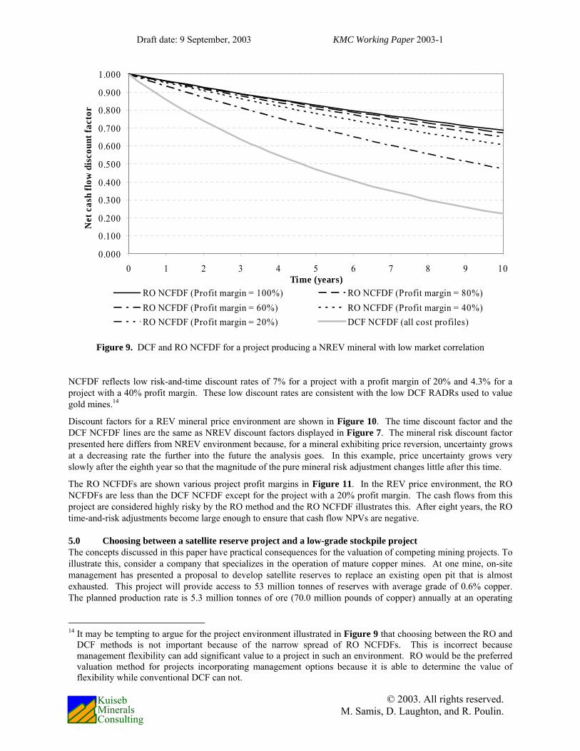
Figure 9 illustrates possible RO NCFDF for projects producing a mineral, such as gold, that is non-reverting and has a low correlation with uncertainty in the overall financial markets. The mineral risk discount factor is calculated with the formula from Equation 12 and a pure mineral risk adjustment rate of 0.75%. This rate is under 1% because of the low correlation (set to 0.1 in this example) between mineral price and financial market uncertainty. The RO

13 The reversion risk discount factor used in this paper is ( )tMineralPRiskRiskDF exp 1 e γσ

γ−⎡ ⎤⋅

= − ⋅ −⎢ ⎥⎣ ⎦

where

PRiskMineral is the price of mineral risk (set to 0.4), σ is the standard deviation of mineral price uncertainty (set to 15%), and γ is a mineral reversion factor (set to 0.231). Other reverting mineral price models will use different risk discount factor formulas. Further details about the risk discounting factor used in this paper can be found in Laughton and Jacoby (1993), Salahor (1998), and Samis (2000).




Figure 7. DCF and RO discounting factors for the NREV price environment.

Figure 8. DCF and RO NCFDF for the NREV price environment.

0.000

0.100

0.200

0.300

0.400

0.500

0.600

0.700

0.800

0.900

1.000

0 1 2 3 4 5 6 7 8 9 10Time (years)

Dis

coun

t fac

tor

RO revenue risk discount factor RO time discount factorRO revenue time+risk discount factor DCF net cash flow discount factor

-1.000

-0.800

-0.600

-0.400

-0.200

0.000

0.200

0.400

0.600

0.800

1.000

0 1 2 3 4 5 6 7 8 9 10

Time (years)

Net

cas

h flo

w d

isco

unt f

acto

r

RO NCFDF (Profit margin = 100%) RO NCFDF (Profit margin = 80%)RO NCFDF (Profit margin = 60%) RO NCFDF (Profit margin = 40%)RO NCFDF (Profit margin = 20%) DCF NCFDF (all cost profiles)




Figure 9. DCF and RO NCFDF for a project producing a NREV mineral with low market correlation

NCFDF reflects low risk-and-time discount rates of 7% for a project with a profit margin of 20% and 4.3% for a project with a 40% profit margin. These low discount rates are consistent with the low DCF RADRs used to value gold mines.14

Discount factors for a REV mineral price environment are shown in Figure 10. The time discount factor and the DCF NCFDF lines are the same as NREV discount factors displayed in Figure 7. The mineral risk discount factor presented here differs from NREV environment because, for a mineral exhibiting price reversion, uncertainty grows at a decreasing rate the further into the future the analysis goes. In this example, price uncertainty grows very slowly after the eighth year so that the magnitude of the pure mineral risk adjustment changes little after this time.

The RO NCFDFs are shown various project profit margins in Figure 11. In the REV price environment, the RO NCFDFs are less than the DCF NCFDF except for the project with a 20% profit margin. The cash flows from this project are considered highly risky by the RO method and the RO NCFDF illustrates this. After eight years, the RO time-and-risk adjustments become large enough to ensure that cash flow NPVs are negative.

5.0 Choosing between a satellite reserve project and a low-grade stockpile project The concepts discussed in this paper have practical consequences for the valuation of competing mining projects. To illustrate this, consider a company that specializes in the operation of mature copper mines. At one mine, on-site management has presented a proposal to develop satellite reserves to replace an existing open pit that is almost exhausted. This project will provide access to 53 million tonnes of reserves with average grade of 0.6% copper. The planned production rate is 5.3 million tonnes of ore (70.0 million pounds of copper) annually at an operating

14 It may be tempting to argue for the project environment illustrated in Figure 9 that choosing between the RO and

DCF methods is not important because of the narrow spread of RO NCFDFs. This is incorrect because management flexibility can add significant value to a project in such an environment. RO would be the preferred valuation method for projects incorporating management options because it is able to determine the value of flexibility while conventional DCF can not.

0.000

0.100

0.200

0.300

0.400

0.500

0.600

0.700

0.800

0.900

1.000

0 1 2 3 4 5 6 7 8 9 10Time (years)

Net

cas

h flo

w d

isco

unt f

acto

r





Figure 10. DCF and RO discounting factors for the REV price environment.

Figure 11. DCF and RO NCFDF for the REV price environment.

0.000

0.100

0.200

0.300

0.400

0.500

0.600

0.700

0.800

0.900

1.000

0 1 2 3 4 5 6 7 8 9 10Time (years)

Dis

coun

t fac

tor

RO revenue risk discount factor RO time discount factor

RO revenue time+risk discount factor DCF net cash flow discount factor

-0.200

0.000

0.200

0.400

0.600

0.800

1.000

0 1 2 3 4 5 6 7 8 9 10

Time (years)

Net

cas

h flo

w d

isco

unt f

acto

r





cost of $0.50 per pound. The satellite reserves will require an initial capital expenditure of $35 million to develop roads to the site, remove the overburden, and complete the mill modifications necessary to handle the new reserves.

There is a competing project from another mine site that has also nearly depleted its reserves. Management at this mine are proposing to extend the life of their mine by using their milling and heap leach facilities to process several low-grade stockpiles from neighboring mines. These stockpiles contain 166 million tonnes of material with an average grade of 0.3% copper. The annual production rate is expected to be 16.6 million tonnes of low-grade material (110 million pounds of copper) at an operating cost of $0.65 per pound of copper. The capital expenditure necessary to develop this project is $10.0 million.

The current copper price is $0.75 per pound. A corporate economist has developed a copper price forecast and a risk-adjustment model that is displayed in Table 3.15 The copper price is expected to rise over the next 10 years to $0.92 per pound while the risk-adjusted (forward) prices associated with this forecast rise more slowly to $0.78 per pound. Note that publicly available copper forward curves only exist for periods of up to two years so that the forward curve must be estimated after this time. The riskless interest rate is assumed to be a constant 3% and the DCF RADR used by the company is 12%.

Unfortunately, only one of these projects can be developed because investment capital is limited. The company’s cash flow is constrained due to the current copper price and the investment bankers who would normally provide project finance are unwilling to increase their exposure to this particular company. Which project should be developed?

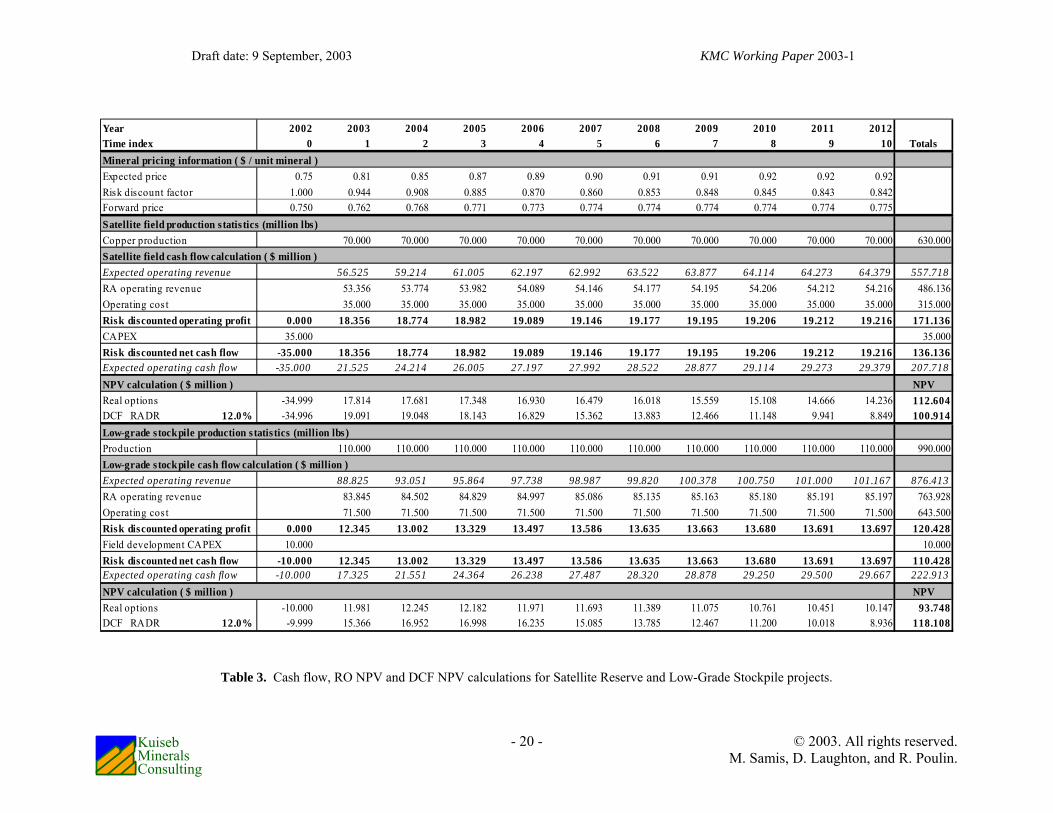
The DCF valuation with an RADR of 12% of both projects is presented in Table 3. Expected operating revenue is calculated by multiplying mineral production by the expected copper price. Operating costs and capital expenditure is subtracted from revenue to provide expected net operating cash flow. These net cash flows are then continuously discounted at 12% to determine the project’s DCF net present value. The DCF NPV for the satellite reserve project is $100.9 million and $118.1 million for the low-grade stockpile project. The low-grade stockpile project is the preferred project when the DCF method is used.

Table 3 also outlines the RO value calculation. Mineral production is multiplied by the risk-adjusted expected copper price to produce risk-adjusted expected revenue. Risk-adjusted net operating cash flow is calculated by subtracting operating costs and capital expenditure from the risk-adjusted revenue. The RO present value of each cash flow is determined by continuously discounting at 3%. The RO NPV for the satellite reserve project is $112.6method is used.

The reason for the different investment recommendations is the relative abilities of DCF and RO methods to assess the risk characteristics of each project. The low-grade stockpile project has higher unit costs than the satellite reserve project so its net cash flow is more risky. This difference in risk manifests itself when using the RO method

by subjecting the stockpile project to a larger effective net cash flow risk adjustment (the revenue risk-adjustment is the same for both projects) and producing a smaller RO NCFDF than the satellite reserve project. Using a 12% DCF RADR, both projects are subject to the same risk-and-time adjustment and have the same NCFDF. Figure 12 presents the DCF and RO NCFDF for both projects. In comparison to the RO NCFDF, the DCF method applies to the satellite reserve cash flows a risk-adjustment that is too large and a risk-adjustment that is too small to the low-grade stockpile cash flows. This results in the DCF method undervaluing the satellite reserves and overvaluing the low-grade stockpiles.

These results are calculated without considering the value of flexibility. Abandonment and temporarily closure options allow management to limit or avoid downside losses which can reduce project risk dramatically. It is possible that low-grade stockpile project includes options which allow its managers to avoid losses more easily than the satellite reserve project. In such a situation, the reduced exposure to financial losses in periods of low mineral 15 The formulas used to calculate copper’s expected and forward price can be found in Jacoby and Laughton (1992),

Salahor (1998) or Samis (2000). These prices where produced using short-term price standard deviation of 25%, a long-term copper price median of $0.90, a copper price reversion factor of 0.4, and a price of copper risk of 0.4. This is a single-factor copper price model that does not always fit actual market data and is used here to reduce the complexity of the example. Multi-factor copper price models are provided in Schwartz (1998) and are used in McCarthy and Monkhouse (forthcoming).


- 20 - © 2003. All rights reserved. M. Samis, D. Laughton, and R. Poulin.


Table 3. Cash flow, RO NPV and DCF NPV calculations for Satellite Reserve and Low-Grade Stockpile projects.

Year 2002 2003 2004 2005 2006 2007 2008 2009 2010 2011 2012Time index 0 1 2 3 4 5 6 7 8 9 10 TotalsMineral pricing information ( $ / unit mineral )Expected price 0.75 0.81 0.85 0.87 0.89 0.90 0.91 0.91 0.92 0.92 0.92Risk discount factor 1.000 0.944 0.908 0.885 0.870 0.860 0.853 0.848 0.845 0.843 0.842Forward price 0.750 0.762 0.768 0.771 0.773 0.774 0.774 0.774 0.774 0.774 0.775Satellite field production statis tics (million lbs)Copper production 70.000 70.000 70.000 70.000 70.000 70.000 70.000 70.000 70.000 70.000 630.000Satellite field cash flow calculation ( $ million )Expected operating revenue 56.525 59.214 61.005 62.197 62.992 63.522 63.877 64.114 64.273 64.379 557.718RA operating revenue 53.356 53.774 53.982 54.089 54.146 54.177 54.195 54.206 54.212 54.216 486.136Operating cos t 35.000 35.000 35.000 35.000 35.000 35.000 35.000 35.000 35.000 35.000 315.000Risk discounted operating profit 0.000 18.356 18.774 18.982 19.089 19.146 19.177 19.195 19.206 19.212 19.216 171.136CAPEX 35.000 35.000Risk discounted net cash flow -35.000 18.356 18.774 18.982 19.089 19.146 19.177 19.195 19.206 19.212 19.216 136.136Expected operating cash flow -35.000 21.525 24.214 26.005 27.197 27.992 28.522 28.877 29.114 29.273 29.379 207.718NPV calculation ( $ million ) NPVReal options -34.999 17.814 17.681 17.348 16.930 16.479 16.018 15.559 15.108 14.666 14.236 112.604DCF RADR 12.0% -34.996 19.091 19.048 18.143 16.829 15.362 13.883 12.466 11.148 9.941 8.849 100.914Low-grade stockpile production s tatistics (million lbs)Production 110.000 110.000 110.000 110.000 110.000 110.000 110.000 110.000 110.000 110.000 990.000Low-grade stockpile cash flow calculation ( $ million )Expected operating revenue 88.825 93.051 95.864 97.738 98.987 99.820 100.378 100.750 101.000 101.167 876.413RA operating revenue 83.845 84.502 84.829 84.997 85.086 85.135 85.163 85.180 85.191 85.197 763.928Operating cos t 71.500 71.500 71.500 71.500 71.500 71.500 71.500 71.500 71.500 71.500 643.500Risk discounted operating profit 0.000 12.345 13.002 13.329 13.497 13.586 13.635 13.663 13.680 13.691 13.697 120.428Field development CAPEX 10.000 10.000Risk discounted net cash flow -10.000 12.345 13.002 13.329 13.497 13.586 13.635 13.663 13.680 13.691 13.697 110.428Expected operating cash flow -10.000 17.325 21.551 24.364 26.238 27.487 28.320 28.878 29.250 29.500 29.667 222.913NPV calculation ( $ million ) NPVReal options -10.000 11.981 12.245 12.182 11.971 11.693 11.389 11.075 10.761 10.451 10.147 93.748DCF RADR 12.0% -9.999 15.366 16.952 16.998 16.235 15.085 13.785 12.467 11.200 10.018 8.936 118.108




Figure 12. RO and DCF NCFDF for the Satellite Reserve and Low-grade Stockpile projects.

prices or other adverse business conditions may result in the low-grade stockpile project being less risky than the satellite reserve project. The interaction between management flexibility and project risk must be assessed with a more involved valuation model that explicitly incorporates project options.16

5.0 Conclusion Comparisons between the conventional DCF and RO valuation methods often focus on the relative ability of each method to calculate the value added by project flexibility. There is no doubt that determining the value of project options is an important part of any valuation exercise because they may turn a risky project with a negative value into one with more desirable risk characteristics and positive value. As an added benefit, the explicit consideration of project options can alert company managers to possible operating strategies that maximize value in different business environments.

However, the focus on the value of flexibility deflects attention away from a more fundamental difference between conventional DCF and RO. These two valuation methods differ in the manner in which they adjust project cash flows for risk and time. The DCF method applies an aggregate risk-and-time adjustment to net cash flow while the RO method divides this adjustment into components so that risk adjustments are applied to the source of uncertainty and time adjustments are applied to net cash flow stream. It may seem to be inconsequential but the difference in risk discounting is the reason that the RO method can account for the risks of individual project cash flows while the

16 Valuation analysts can use real option or decision tree models to determine the value of project flexibility.

Decision tree models map out possible project outcomes based on underlying project uncertainties and structure. Cash flow outcomes within the tree are valued using their probability of occurrence and DCF discounting (for an overview of decision trees see Clemen, 1996). The results from this paper show that it is incorrect to use a single RADR within a decision tree since project risk changes within the tree. An investor preference relationship function is required to account for these risk variations.

0.000

0.100

0.200

0.300

0.400

0.500

0.600

0.700

0.800

0.900

1.000

0 1 2 3 4 5 6 7 8 9 10Time (years)

Net

cas

h flo

w d

isco

unt f

acto

rs

DCF NCFDF at 12% RO NCFDF satellite reserves RO NCFDF low-grade stockpile




conventional DCF method cannot. This paper has demonstrated the mechanics of conventional DCF and RO risk discounting and shown that the RO method is better able to account for cash flow risk.

The difference in risk discounting is also important because it affects corporate valuation policy. Companies are naturally interested in ensuring that investment capital is allocated efficiently since this will improve return on equity. The efficient allocation of capital requires that the valuation method used for this recognize the factors influencing project value which are the risk and timing of project cash flows. This process can hardly be called effective if projects are valued using a method that is insensitive to or has only limited ability to account for cash flow risk. Thus, it may be more productive for the arguments between advocates of conventional DCF and RO methods to be focused on which method is more capable of accounting for project risk than on their relative abilities to value management flexibility.

References

Brennan, M. and E. Schwartz (1985). “Evaluating natural resource investment.” Journal of Business 58(2): pp. 135-157.

Bradley, P. (1998). “On the use of MAP to compare alternative royalty systems for petroleum development projects.” The Energy Journal 19(1): pp. 47-82.

Clemen, R. (1996). Making Hard Decisions: An Introduction to Decision Analysis - Second Edition. Duxbury Press. New York, NY: 664p.

Giammarino, R., and E. Maynes, R. Brealey, S. Myers, A. Marcus (1996). Fundamentals of Corporate Finance – First Canadian Edition. McGraw-Hill Ryerson Limited. Toronto, ON: 683p.

Hull, J. (2002). Options, Futures and Other Derivatives. Prentice-Hall Inc. Upper Saddle River, NJ: 698p.

Jacoby, H. and D. Laughton (1992). “Project evaluation: A practical asset pricing method.” The Energy Journal 13: pp. 19-47.

Laughton, D. and H. Jacoby (1993). “Reversion, timing options and long-term decision-making.” Financial Management 22(3): pp. 225-240.

McCarthy, J. and P. Monkhouse (forthcoming). “To open or not to open, or what to do with a closed copper mine.” Journal of Applied Corporate Finance.

McDonald, R. and D. Siegel (1985). “Investment and the valuation of firms when there is an option to shut down.” International Economic Review 26(2): pp. 331-349.

Salahor, G. (1998). “Implications of output price risk and operating leverage for the evaluation of petroleum development projects.” The Energy Journal 19(1): pp. 13-46.

Samis, M. (1995). An option pricing analysis of the 1990 capital structure of ERPM. Computer Applications in the Mining Industry - Third Canadian Conference, Montreal, Canada.

Samis, M. (2000). Multi-Zone Mine Valuation Using Modern Asset Pricing (Real Options) Techniques. Unpublished Ph.D. dissertation, Department of Mining and Mineral Process Engineering, University of British Columbia. Vancouver, BC: 161p.

Samis, M., and D. Laughton, R. Poulin (2002). “An example of using real options to model a mine expansion decision at a multi-zone deposit.” 2002 Application of Computers and Operations Research in the Minerals Industry. Phoenix, AZ.

Schwartz, E. (1997). “The stochastic behavior of commodity prices: implications for valuation and hedging.” The Journal of Finance 52(3): pp. 923-973.

Smith, L. (2000). “Discounted cash flow analysis: Methodology and discount rates.” Mineral Property Valuation Proceedings: Papers presented at Mining Millennium 2000. Canadian Institute of Mining, Metallurgy and Petroleum. Montreal, Quebec: pp. 85-100.

Smith, L. (2001). “Financial analysis and economic optimization.” Mineral Processing Plant Design, Practice, and Control: Proceedings. Society of Mining, Metallurgy, and Exploration Inc. Littleton, CO: 2410p.

risk discounting: the fundamental difference between the real option and discounted cash flow...

Documents