how to perform discounted cash flow valuation? - repo pw

Foundations of Management, Vol. 3, No. 1 (2011), ISSN 2080-7279 DOI: 10.2478/v10238-012-0037-4 81

HOW TO PERFORM DISCOUNTED CASH FLOW VALUATION?

Sławomir JANISZEWSKI

Faculty of Management Warsaw University of Technology, Warsaw, Poland

e-mail: [email protected]

Abstract: Within the last few decades the quickly accelerating globalization processes contributed to rapid increase in the value of the global capital markets, and mergers and acquisitions transactions. This implicat-ed the rising importance of methodologies that enable investors to efficiently value the companies. The aim of this elaboration is to present practical approach towards the discounted cash flow company valu-ation method, considered one of the most effective but simultaneously one of the most sophisticated among all. The article comprises purely theoretical as well as practical knowledge, based on the author’s broad pro-fessional experiences.

Key words: valuation, discounted cash flow, free cash flows to firm, free cash flows to equity, residual val-ue, discount rate, beta, market risk premium.

1 Introduction In theory, the fair market value of a company can be assessed only in a real transaction, at which the shares change hands between a willing buyer and a willing seller. In such transaction the buyer is not under any compulsion to buy, the seller is not under any compul-sion to sell and both parties have reasonable knowledge of all relevant facts.

In practice there are few generally accepted methodol-ogy of company valuation which often are

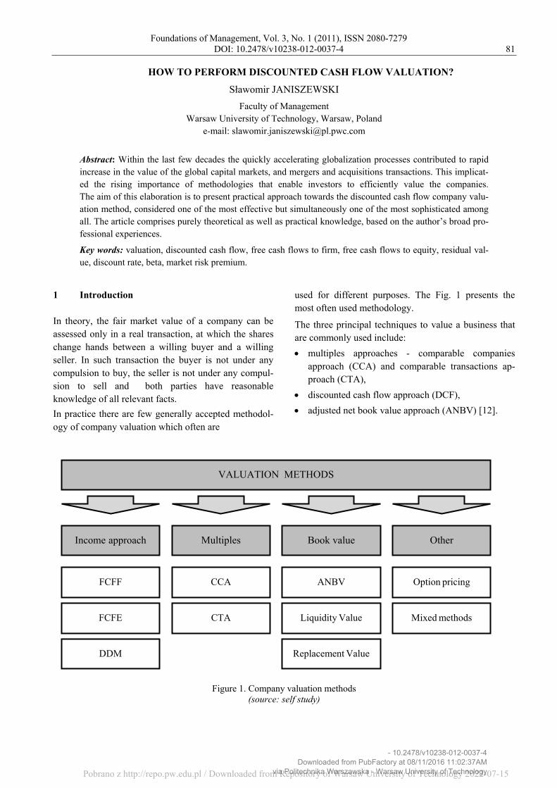
used for different purposes. The Fig. 1 presents the most often used methodology.

The three principal techniques to value a business that are commonly used include:

multiples approaches - comparable companies approach (CCA) and comparable transactions ap-proach (CTA),

discounted cash flow approach (DCF),

adjusted net book value approach (ANBV) [12].

Figure 1. Company valuation methods (source: self study)

VALUATION METHODS

Income approach Other Book value Multiples

CCA

CTA

FCFF

DDM

ANBV

FCFE Liquidity Value

Replacement Value

Option pricing

Mixed methods

- 10.2478/v10238-012-0037-4Downloaded from PubFactory at 08/11/2016 11:02:37AM

via Politechnika Warszawska - Warsaw University of TechnologyPobrano z http://repo.pw.edu.pl / Downloaded from Repository of Warsaw University of Technology 2022-07-15

82 Sławomir Janiszewski

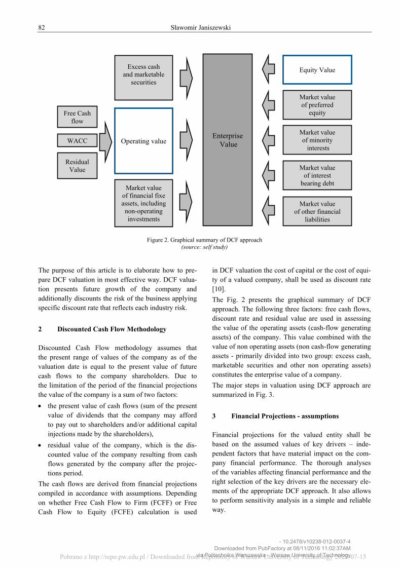
Figure 2. Graphical summary of DCF approach (source: self study)

The purpose of this article is to elaborate how to pre-pare DCF valuation in most effective way. DCF valua-tion presents future growth of the company and additionally discounts the risk of the business applying specific discount rate that reflects each industry risk.

2 Discounted Cash Flow Methodology Discounted Cash Flow methodology assumes that the present range of values of the company as of the valuation date is equal to the present value of future cash flows to the company shareholders. Due to the limitation of the period of the financial projections the value of the company is a sum of two factors:

the present value of cash flows (sum of the present value of dividends that the company may afford to pay out to shareholders and/or additional capital injections made by the shareholders),

residual value of the company, which is the dis-counted value of the company resulting from cash flows generated by the company after the projec-tions period.

The cash flows are derived from financial projections compiled in accordance with assumptions. Depending on whether Free Cash Flow to Firm (FCFF) or Free Cash Flow to Equity (FCFE) calculation is used

in DCF valuation the cost of capital or the cost of equi-ty of a valued company, shall be used as discount rate [10].

The Fig. 2 presents the graphical summary of DCF approach. The following three factors: free cash flows, discount rate and residual value are used in assessing the value of the operating assets (cash-flow generating assets) of the company. This value combined with the value of non operating assets (non cash-flow generating assets - primarily divided into two group: excess cash, marketable securities and other non operating assets) constitutes the enterprise value of a company.

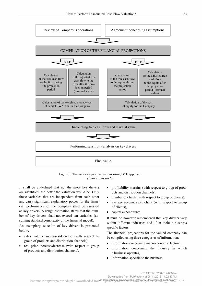
The major steps in valuation using DCF approach are summarized in Fig. 3.

3 Financial Projections - assumptions Financial projections for the valued entity shall be based on the assumed values of key drivers – inde-pendent factors that have material impact on the com-pany financial performance. The thorough analyses of the variables affecting financial performance and the right selection of the key drivers are the necessary ele-ments of the appropriate DCF approach. It also allows to perform sensitivity analysis in a simple and reliable way.

WACC

Residual Value

Free Cash flow

Operating value

Excess cash and marketable

securities

Market value of financial fixe assets, including non-operating investments

Enterprise Value

Equity Value

Market value of preferred

equity

Market value of minority interests

Market value of interest

bearing debt

Market value of other financial

liabilities



How to Perform Discounted Cash Flow Valuation? 83

It shall be underlined that not the more key drivers are identified, the better the valuation would be. Only those variables that are independent from each other and carry significant explanatory power for the finan-cial performance of the company shall be assessed as key drivers. A rough estimation states that the num-ber of key drivers shall not exceed ten variables (as-suming standard complexity of the financial model).

An exemplary selection of key drivers is presented below:

sales volume increases/decrease (with respect to group of products and distribution channels),

real price increase/decrease (with respect to group of products and distribution channels),

profitability margins (with respect to group of prod-ucts and distribution channels),

number of clients (with respect to group of clients),

average revenues per client (with respect to group of clients),

capital expenditures.

It must be however remembered that key drivers vary within different industries and often include business specific factors.

The financial projections for the valued company can be compiled using three categories of information:

information concerning macroeconomic factors,

information concerning the industry in which a business operates,

information specific to the business.

Figure 3. The major steps in valuations using DCF approach (source: self study)

Agreement concerning assumptions Review of Company’s operations

COMPILATION OF THE FINANCIAL PROJECTIONS

Calculation of the cost of equity for the Company

Discounting free cash flow and residual value

Performing sensitivity analysis on key drivers

Final value

Calculation of the free cash flow to the equity during

the projection period

Calculation of the adjusted free

cash flow to the equity after

the projection period (terminal

value)

Calculation of the free cash flow

to the firm during the projection

period

Calculation of the adjusted free

cash flow to the firm after the pro-

jection period (terminal value)

Calculation of the weighted average cost of capital (WACC) for the Company

FCFF FCFE




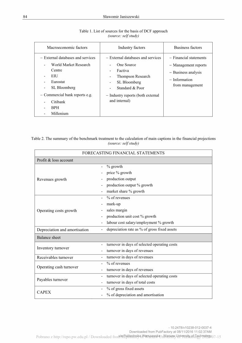
Table 1. List of sources for the basis of DCF approach (source: self study)

Macroeconomic factors Industry factors Business factors

External databases and services

- World Market Research Centre

- EIU

- Eurostat

- SL Bloomberg

Commercial bank reports e.g.

- Citibank

- BPH

- Millenium

External databases and services

- One Source

- Factiva

- Thompson Research

- SL Bloomberg

- Standard & Poor

Industry reports (both external and internal)

Financial statements

Management reports

Business analysis

Information from management

Table 2. The summary of the benchmark treatment to the calculation of main captions in the financial projections (source: self study)

FORECASTING FINANCIAL STATEMENTS

Profit & loss account

Revenues growth

- % growth

- price % growth

- production output

- production output % growth

- market share % growth

Operating costs growth

- % of revenues

- mark-up

- sales margin

- production unit cost % growth

- labour cost salary/employment % growth

Depreciation and amortisation - depreciation rate as % of gross fixed assets

Balance sheet

Inventory turnover - turnover in days of selected operating costs

- turnover in days of revenues

Receivables turnover - turnover in days of revenues

Operating cash turnover - % of revenues

- turnover in days of revenues

Payables turnover - turnover in days of selected operating costs

- turnover in days of total costs

CAPEX - % of gross fixed assets

- % of depreciation and amortisation




In general information on the macroeconomic factors and industry specific factors might be obtained from publicly available sources whereas the information on the factors specific to the valued entity shall be pri-marily provided by the management of the company.

The list of the sources which might constitute the basis for DCF approach valuation is presented in Table 1.

Set of assumptions shall provide both the information on the values of key parameters of the model and on the methodology of calculation of the certain cap-tions in the financial projections.

The summary of the benchmark treatment to the calcu-lation of main captions in the financial projections is presented in Table 2.

The duration of the financial projections shall be heavi-ly dependent on the forecasted performance of the val-ued entity. The general rule is that the duration of financial projections shall be at least equal to the period in which the company is supposed to reach the stable growth in perpetuity. The financial projec-tions shall cover the period long enough to estimate a normalised or mature level of cash flows prior to deriving to terminal value. The residual value shall be calculated no earlier than when steady state of the business’ operations arrives – this implies that all the value drivers in the financial projections would remain constant [12, 4].

In spite of the fact that while projections become less reliable further out, it still may be necessary to go out up to 10 years or more in order to reach normalised levels. Furthermore, if the valued company is expected to have a competitive advantage for a certain period, the financial projections duration should be of suffi-cient length to capture the entire period of this competi-tive advantage.

Summary of the factors that are useful in determining the duration of financial projections for the purposes of DCF valuation is presented below:

the length of high growth or transition growth peri-od,

industry cycle and competitive structure (operating margins),

economic cycle,

knowledge of significant events,

useful life of assets (e.g. coal, oil, etc.),

comfort of the person responsible for the assump-tions,

length of any competitive advantage.

It is important to remember that usually longer finan-cial projections period allows reducing the impact of the residual value on the valuation results. It is im-portant argument for extending the period of financial projections – the vogue estimate is that residual value shall constitute no more than 50,0% of the company value. In other cases the valuation result becomes very sensitive for the changes in projected cash flow in the last year of financial projections, which is the base to calculate the residual value [2].

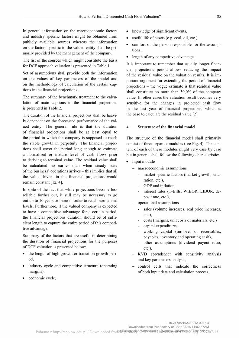
4 Structure of the financial model The structure of the financial model shall primarily consist of three separate modules (see Fig. 4). The con-tent of each of these modules might very case by case but in general shall follow the following characteristic:

Input module

macroeconomic assumptions

- market specific factors (market growth, satu-ration, etc.),

- GDP and inflation, - interest rates (T-Bills, WIBOR, LIBOR, de-

posit rate, etc.),

operational assumptions

- sales (volume increases, real price increases, etc.),

- costs (margins, unit costs of materials, etc.) - capital expenditures, - working capital (turnover of receivables,

payables, inventory and operating cash), - other assumptions (dividend payout ratio,

etc.),

KVD spreadsheet with sensitivity analysis and key parameters analysis,

control cells that indicate the correctness of both input data and calculation process.




Figure 4. The structure of financial model (source: self study)

Calculation module

calculating formulas and performing conversion of input/output variables:

- calculation of sales revenues (division of sales in respect to products and distribu-tion channels),

- calculation of cost by nature (materials & energy, depreciation, external services, payroll, etc.),

should not include sensitivity analysis and statis-tical tests,

should not include input cells (input data).

Output module

presentation of the final results on the aggregat-ed level:

- profit and loss account,

- balance sheet,

- cash flow statement,

presentation of additional measures of financial performance:

- sales and operating costs analytics,

- ratio analysis.

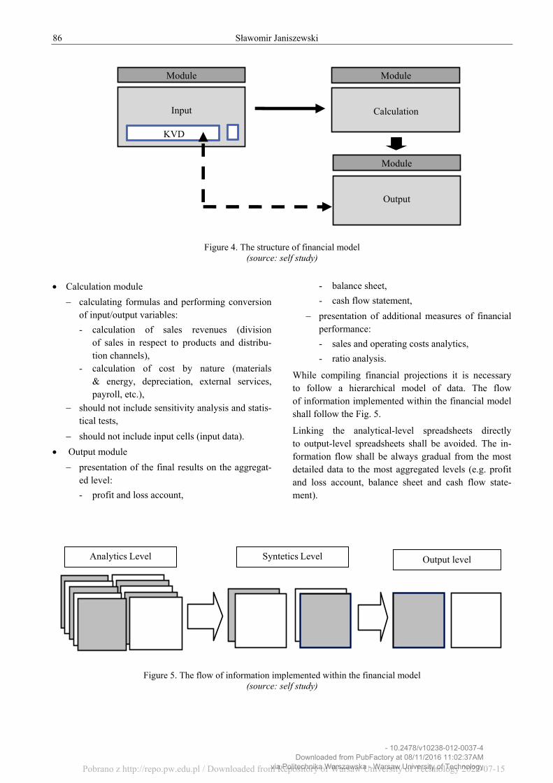
While compiling financial projections it is necessary to follow a hierarchical model of data. The flow of information implemented within the financial model shall follow the Fig. 5.

Linking the analytical-level spreadsheets directly to output-level spreadsheets shall be avoided. The in-formation flow shall be always gradual from the most detailed data to the most aggregated levels (e.g. profit and loss account, balance sheet and cash flow state-ment).

Figure 5. The flow of information implemented within the financial model (source: self study)

Output level Syntetics Level Analytics Level

Module

Input

KVD

Module

Module Module

Calculation

ModuleModule

Output




EBIT Earnings Before Interest and Taxes – the figure derived from Profit and Loss account (adjusted for extraordinary items)

+

Depreciation and amortisation Depreciation of all tangible and intangible assets (separate treatmentof goodwill amortization might be considered) - the figure derived from P&L

+

Corporate Income Tax paid (-) The figure derived from Profit and Loss account adjusted for Balance Sheet captions – deferred tax asset/liability unless additional CIT calcula-tion spreadsheet is available

= GROSS CASH-FLOWS

+

Changes in Working Capital Usually split into following categories: changes in operating cash, receivables, payables and inventory - the figures derived from Balance Sheet

+

Changes in other assets and liabilities Usually split into following categories: prepayments, financial assets (excluding cash), reserves and accruals excluding changes in deferred tax asset/liabilities - the figures derived from Balance Sheet

=

OPERATING CASH-FLOWS

+

Capital Expenditures (-) This caption might be split into two categories: replacement capital ex-penditures and expansion capital expenditures - the figures derived from Fixed Assets summary spreadsheet

+ CASH-FLOWS BEFORE FINANCING

+

Change in Indebtedness The difference between the debt issues and debt repayments - the figures derived from Balance Sheet

+

Net Interest The difference between the interest revenue and interest expense the figure derived from Profit and Loss account

= FREE CASH-FLOWS TO EQUITY

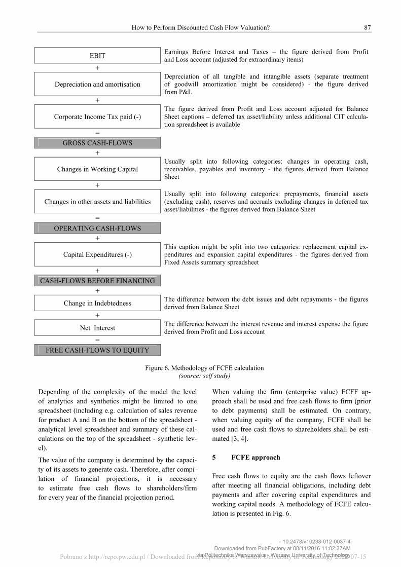
Figure 6. Methodology of FCFE calculation

(source: self study)

Depending of the complexity of the model the level of analytics and synthetics might be limited to one spreadsheet (including e.g. calculation of sales revenue for product A and B on the bottom of the spreadsheet - analytical level spreadsheet and summary of these cal-culations on the top of the spreadsheet - synthetic lev-el).

The value of the company is determined by the capaci-ty of its assets to generate cash. Therefore, after compi-lation of financial projections, it is necessary to estimate free cash flows to shareholders/firm for every year of the financial projection period.

When valuing the firm (enterprise value) FCFF ap-proach shall be used and free cash flows to firm (prior to debt payments) shall be estimated. On contrary, when valuing equity of the company, FCFE shall be used and free cash flows to shareholders shall be esti-mated [3, 4]. 5 FCFE approach Free cash flows to equity are the cash flows leftover after meeting all financial obligations, including debt payments and after covering capital expenditures and working capital needs. A methodology of FCFE calcu-lation is presented in Fig. 6.




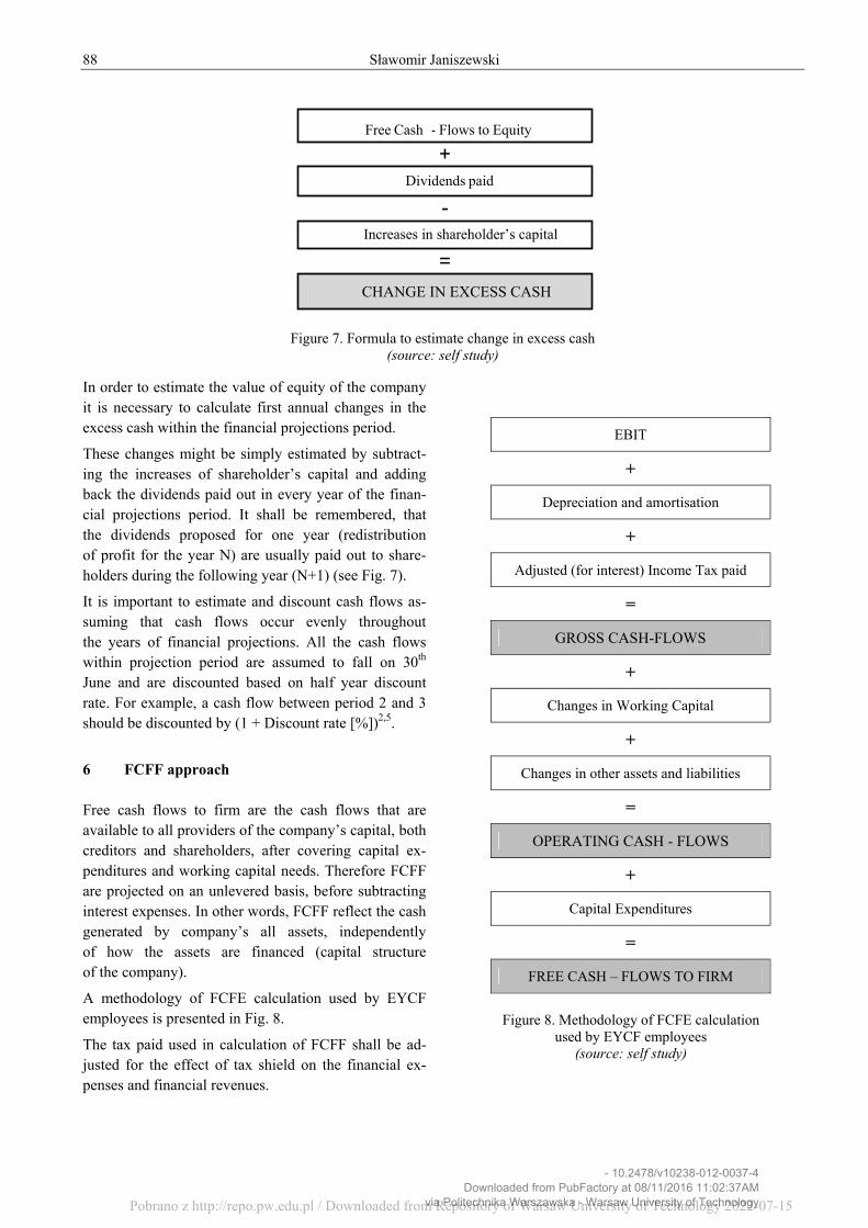
Figure 7. Formula to estimate change in excess cash (source: self study)

In order to estimate the value of equity of the company it is necessary to calculate first annual changes in the excess cash within the financial projections period.

These changes might be simply estimated by subtract-ing the increases of shareholder’s capital and adding back the dividends paid out in every year of the finan-cial projections period. It shall be remembered, that the dividends proposed for one year (redistribution of profit for the year N) are usually paid out to share-holders during the following year (N+1) (see Fig. 7).

It is important to estimate and discount cash flows as-suming that cash flows occur evenly throughout the years of financial projections. All the cash flows within projection period are assumed to fall on 30th June and are discounted based on half year discount rate. For example, a cash flow between period 2 and 3 should be discounted by (1 + Discount rate [%])2,5.

6 FCFF approach Free cash flows to firm are the cash flows that are available to all providers of the company’s capital, both creditors and shareholders, after covering capital ex-penditures and working capital needs. Therefore FCFF are projected on an unlevered basis, before subtracting interest expenses. In other words, FCFF reflect the cash generated by company’s all assets, independently of how the assets are financed (capital structure of the company).

A methodology of FCFE calculation used by EYCF employees is presented in Fig. 8.

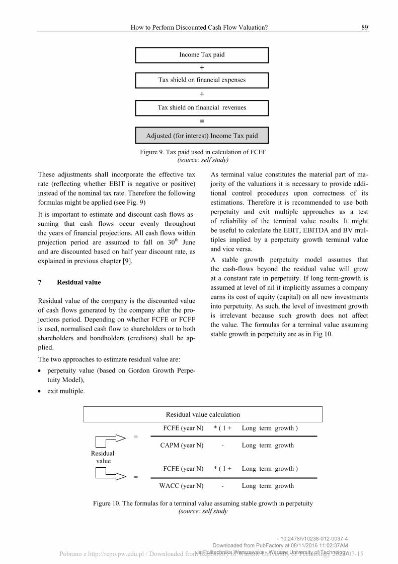
The tax paid used in calculation of FCFF shall be ad-justed for the effect of tax shield on the financial ex-penses and financial revenues.

Figure 8. Methodology of FCFE calculation used by EYCF employees


=

-

CHANGE IN EXCESS CASH

+Dividends paid

Increases in shareholder’s capital

Free Cash ‐ Flows to Equity

EBIT

+

Depreciation and amortisation

+

Adjusted (for interest) Income Tax paid

=

GROSS CASH-FLOWS

+

Changes in Working Capital

+

Changes in other assets and liabilities

=

OPERATING CASH - FLOWS

+

Capital Expenditures

=

FREE CASH – FLOWS TO FIRM




Figure 9. Tax paid used in calculation of FCFF (source: self study)

These adjustments shall incorporate the effective tax rate (reflecting whether EBIT is negative or positive) instead of the nominal tax rate. Therefore the following formulas might be applied (see Fig. 9)

It is important to estimate and discount cash flows as-suming that cash flows occur evenly throughout the years of financial projections. All cash flows within projection period are assumed to fall on 30th June and are discounted based on half year discount rate, as explained in previous chapter [9].

7 Residual value Residual value of the company is the discounted value of cash flows generated by the company after the pro-jections period. Depending on whether FCFE or FCFF is used, normalised cash flow to shareholders or to both shareholders and bondholders (creditors) shall be ap-plied.

The two approaches to estimate residual value are:

perpetuity value (based on Gordon Growth Perpe-tuity Model),

exit multiple.

As terminal value constitutes the material part of ma-jority of the valuations it is necessary to provide addi-tional control procedures upon correctness of its estimations. Therefore it is recommended to use both perpetuity and exit multiple approaches as a test of reliability of the terminal value results. It might be useful to calculate the EBIT, EBITDA and BV mul-tiples implied by a perpetuity growth terminal value and vice versa.

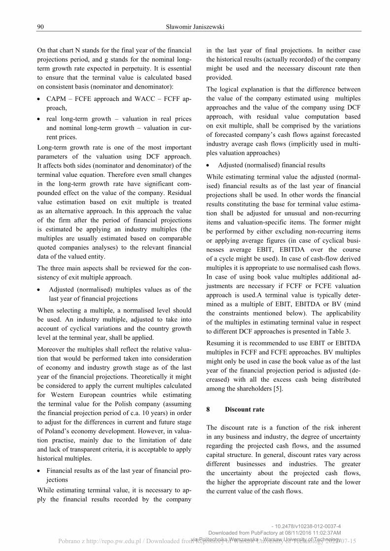
A stable growth perpetuity model assumes that the cash-flows beyond the residual value will grow at a constant rate in perpetuity. If long term-growth is assumed at level of nil it implicitly assumes a company earns its cost of equity (capital) on all new investments into perpetuity. As such, the level of investment growth is irrelevant because such growth does not affect the value. The formulas for a terminal value assuming stable growth in perpetuity are as in Fig 10.

Residual value calculation

Residual value

FCFE (year N) * ( 1 + Long term growth ) =

CAPM (year N) - Long term growth

FCFE (year N) * ( 1 + Long term growth ) =

WACC (year N) - Long term growth

Figure 10. The formulas for a terminal value assuming stable growth in perpetuity (source: self study

=

Adjusted (for interest) Income Tax paid

+

Tax shield on financial expenses

Tax shield on financial revenues

+

Income Tax paid




On that chart N stands for the final year of the financial projections period, and g stands for the nominal long-term growth rate expected in perpetuity. It is essential to ensure that the terminal value is calculated based on consistent basis (nominator and denominator):

CAPM – FCFE approach and WACC – FCFF ap-proach,

real long-term growth – valuation in real prices and nominal long-term growth – valuation in cur-rent prices.

Long-term growth rate is one of the most important parameters of the valuation using DCF approach. It affects both sides (nominator and denominator) of the terminal value equation. Therefore even small changes in the long-term growth rate have significant com-pounded effect on the value of the company. Residual value estimation based on exit multiple is treated as an alternative approach. In this approach the value of the firm after the period of financial projections is estimated be applying an industry multiples (the multiples are usually estimated based on comparable quoted companies analyses) to the relevant financial data of the valued entity.

The three main aspects shall be reviewed for the con-sistency of exit multiple approach.

Adjusted (normalised) multiples values as of the last year of financial projections

When selecting a multiple, a normalised level should be used. An industry multiple, adjusted to take into account of cyclical variations and the country growth level at the terminal year, shall be applied.

Moreover the multiples shall reflect the relative valua-tion that would be performed taken into consideration of economy and industry growth stage as of the last year of the financial projections. Theoretically it might be considered to apply the current multiples calculated for Western European countries while estimating the terminal value for the Polish company (assuming the financial projection period of c.a. 10 years) in order to adjust for the differences in current and future stage of Poland’s economy development. However, in valua-tion practise, mainly due to the limitation of date and lack of transparent criteria, it is acceptable to apply historical multiples.

Financial results as of the last year of financial pro-jections

While estimating terminal value, it is necessary to ap-ply the financial results recorded by the company

in the last year of final projections. In neither case the historical results (actually recorded) of the company might be used and the necessary discount rate then provided.

The logical explanation is that the difference between the value of the company estimated using multiples approaches and the value of the company using DCF approach, with residual value computation based on exit multiple, shall be comprised by the variations of forecasted company’s cash flows against forecasted industry average cash flows (implicitly used in multi-ples valuation approaches)

Adjusted (normalised) financial results

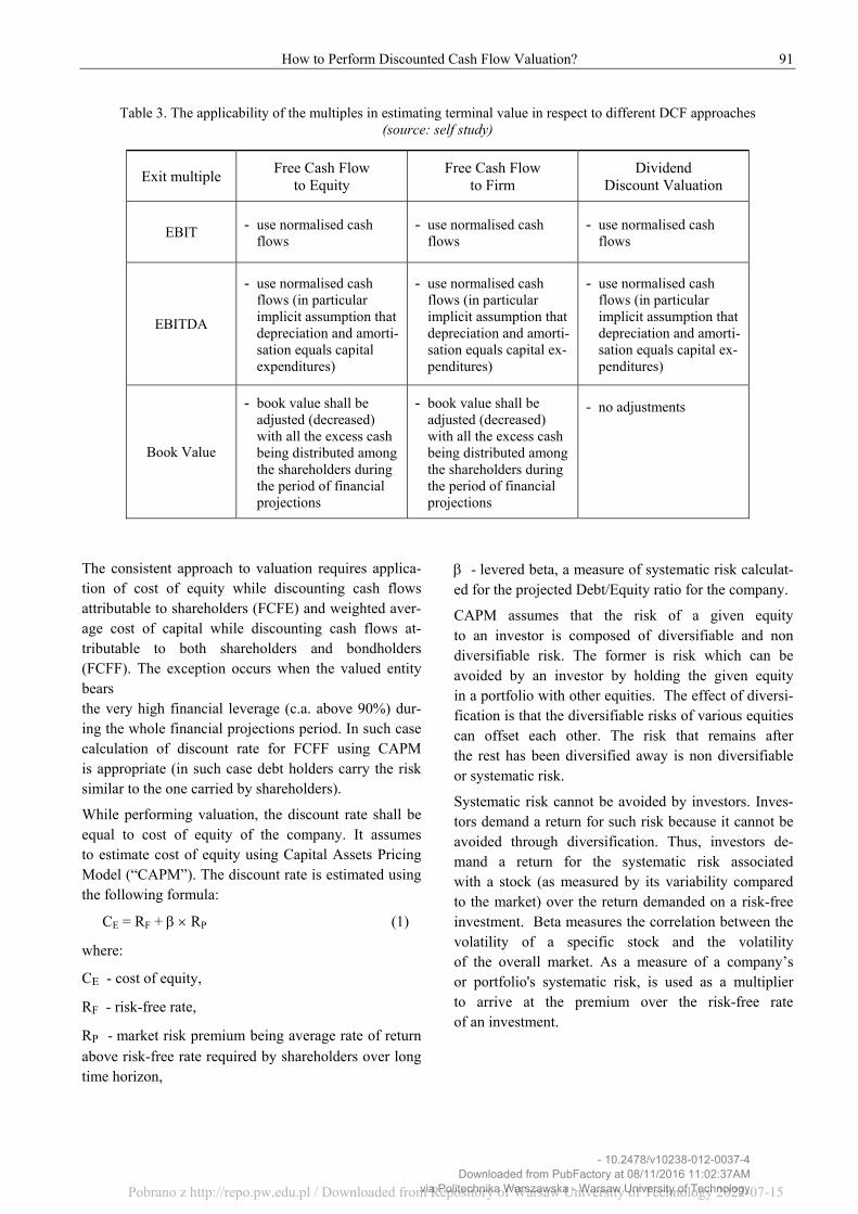
While estimating terminal value the adjusted (normal-ised) financial results as of the last year of financial projections shall be used. In other words the financial results constituting the base for terminal value estima-tion shall be adjusted for unusual and non-recurring items and valuation-specific items. The former might be performed by either excluding non-recurring items or applying average figures (in case of cyclical busi-nesses average EBIT, EBITDA over the course of a cycle might be used). In case of cash-flow derived multiples it is appropriate to use normalised cash flows. In case of using book value multiples additional ad-justments are necessary if FCFF or FCFE valuation approach is used.A terminal value is typically deter-mined as a multiple of EBIT, EBITDA or BV (mind the constraints mentioned below). The applicability of the multiples in estimating terminal value in respect to different DCF approaches is presented in Table 3.

Resuming it is recommended to use EBIT or EBITDA multiples in FCFF and FCFE approaches. BV multiples might only be used in case the book value as of the last year of the financial projection period is adjusted (de-creased) with all the excess cash being distributed among the shareholders [5].

8 Discount rate The discount rate is a function of the risk inherent in any business and industry, the degree of uncertainty regarding the projected cash flows, and the assumed capital structure. In general, discount rates vary across different businesses and industries. The greater the uncertainty about the projected cash flows, the higher the appropriate discount rate and the lower the current value of the cash flows.




Table 3. The applicability of the multiples in estimating terminal value in respect to different DCF approaches (source: self study)

The consistent approach to valuation requires applica-tion of cost of equity while discounting cash flows attributable to shareholders (FCFE) and weighted aver-age cost of capital while discounting cash flows at-tributable to both shareholders and bondholders (FCFF). The exception occurs when the valued entity bears the very high financial leverage (c.a. above 90%) dur-ing the whole financial projections period. In such case calculation of discount rate for FCFF using CAPM is appropriate (in such case debt holders carry the risk similar to the one carried by shareholders).

While performing valuation, the discount rate shall be equal to cost of equity of the company. It assumes to estimate cost of equity using Capital Assets Pricing Model (“CAPM”). The discount rate is estimated using the following formula:

CE = RF + RP (1)

where:

CE - cost of equity,

RF - risk-free rate,

RP - market risk premium being average rate of return above risk-free rate required by shareholders over long time horizon,

- levered beta, a measure of systematic risk calculat-ed for the projected Debt/Equity ratio for the company.

CAPM assumes that the risk of a given equity to an investor is composed of diversifiable and non diversifiable risk. The former is risk which can be avoided by an investor by holding the given equity in a portfolio with other equities. The effect of diversi-fication is that the diversifiable risks of various equities can offset each other. The risk that remains after the rest has been diversified away is non diversifiable or systematic risk.

Systematic risk cannot be avoided by investors. Inves-tors demand a return for such risk because it cannot be avoided through diversification. Thus, investors de-mand a return for the systematic risk associated with a stock (as measured by its variability compared to the market) over the return demanded on a risk-free investment. Beta measures the correlation between the volatility of a specific stock and the volatility of the overall market. As a measure of a company’s or portfolio's systematic risk, is used as a multiplier to arrive at the premium over the risk-free rate of an investment.

Exit multiple Free Cash Flow

to Equity Free Cash Flow

to Firm Dividend

Discount Valuation

EBIT - use normalised cash flows

- use normalised cash flows

- use normalised cash flows

EBITDA

- use normalised cash flows (in particular implicit assumption that depreciation and amorti-sation equals capital expenditures)

- use normalised cash flows (in particular implicit assumption that depreciation and amorti-sation equals capital ex-penditures)

- use normalised cash flows (in particular implicit assumption that depreciation and amorti-sation equals capital ex-penditures)

Book Value

- book value shall be adjusted (decreased) with all the excess cash being distributed among the shareholders during the period of financial projections

- book value shall be adjusted (decreased) with all the excess cash being distributed among the shareholders during the period of financial projections

- no adjustments




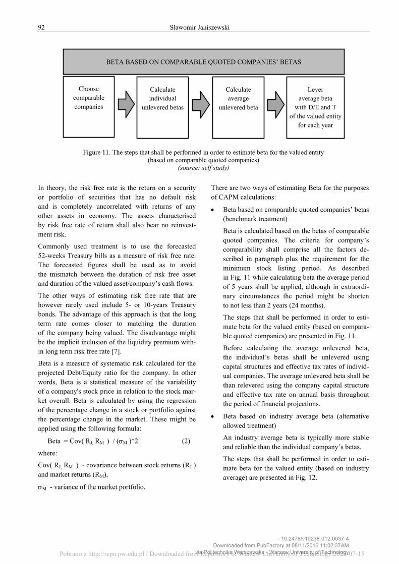
Figure 11. The steps that shall be performed in order to estimate beta for the valued entity (based on comparable quoted companies)


In theory, the risk free rate is the return on a security or portfolio of securities that has no default risk and is completely uncorrelated with returns of any other assets in economy. The assets characterised by risk free rate of return shall also bear no reinvest-ment risk.

Commonly used treatment is to use the forecasted 52-weeks Treasury bills as a measure of risk free rate. The forecasted figures shall be used as to avoid the mismatch between the duration of risk free asset and duration of the valued asset/company’s cash flows.

The other ways of estimating risk free rate that are however rarely used include 5- or 10-years Treasury bonds. The advantage of this approach is that the long term rate comes closer to matching the duration of the company being valued. The disadvantage might be the implicit inclusion of the liquidity premium with-in long term risk free rate [7].

Beta is a measure of systematic risk calculated for the projected Debt/Equity ratio for the company. In other words, Beta is a statistical measure of the variability of a company's stock price in relation to the stock mar-ket overall. Beta is calculated by using the regression of the percentage change in a stock or portfolio against the percentage change in the market. These might be applied using the following formula:

Beta = Cov( RJ, RM ) / (M )^2 (2)

where:

Cov( RJ, RM ) - covariance between stock returns (RJ ) and market returns (RM),

M - variance of the market portfolio.

There are two ways of estimating Beta for the purposes of CAPM calculations:

Beta based on comparable quoted companies’ betas (benchmark treatment)

Beta is calculated based on the betas of comparable quoted companies. The criteria for company’s comparability shall comprise all the factors de-scribed in paragraph plus the requirement for the minimum stock listing period. As described in Fig. 11 while calculating beta the average period of 5 years shall be applied, although in extraordi-nary circumstances the period might be shorten to not less than 2 years (24 months).

The steps that shall be performed in order to esti-mate beta for the valued entity (based on compara-ble quoted companies) are presented in Fig. 11.

Before calculating the average unlevered beta, the individual’s betas shall be unlevered using capital structures and effective tax rates of individ-ual companies. The average unlevered beta shall be than relevered using the company capital structure and effective tax rate on annual basis throughout the period of financial projections.

Beta based on industry average beta (alternative allowed treatment)

An industry average beta is typically more stable and reliable than the individual company’s betas.

The steps that shall be performed in order to esti-mate beta for the valued entity (based on industry average) are presented in Fig. 12.

B ’

Choose comparable companies

Calculate individual

unlevered betas

Calculate average

unlevered beta

Lever average beta

with D/E and T of the valued entity

for each year

BETA BASED ON COMPARABLE QUOTED COMPANIES’ BETAS




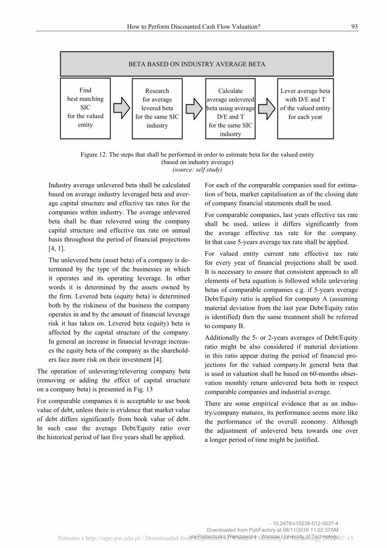
Figure 12. The steps that shall be performed in order to estimate beta for the valued entity

(based on industry average) (source: self study)

Industry average unlevered beta shall be calculated based on average industry leveraged beta and aver-age capital structure and effective tax rates for the companies within industry. The average unlevered beta shall be than relevered using the company capital structure and effective tax rate on annual basis throughout the period of financial projections [4, 1].

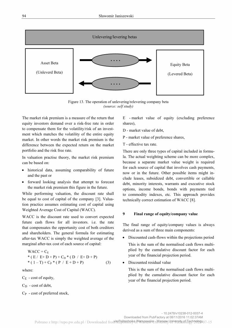
The unlevered beta (asset beta) of a company is de-termined by the type of the businesses in which it operates and its operating leverage. In other words it is determined by the assets owned by the firm. Levered beta (equity beta) is determined both by the riskiness of the business the company operates in and by the amount of financial leverage risk it has taken on. Levered beta (equity) beta is affected by the capital structure of the company. In general an increase in financial leverage increas-es the equity beta of the company as the sharehold-ers face more risk on their investment [4].

The operation of unlevering/relevering company beta (removing or adding the effect of capital structure on a company beta) is presented in Fig. 13

For comparable companies it is acceptable to use book value of debt, unless there is evidence that market value of debt differs significantly from book value of debt. In such case the average Debt/Equity ratio over the historical period of last five years shall be applied.

For each of the comparable companies used for estima-tion of beta, market capitalisation as of the closing date of company financial statements shall be used.

For comparable companies, last years effective tax rate shall be used, unless it differs significantly from the average effective tax rate for the company. In that case 5-years average tax rate shall be applied.

For valued entity current rate effective tax rate for every year of financial projections shall be used. It is necessary to ensure that consistent approach to all elements of beta equation is followed while unlevering betas of comparable companies e.g. if 5-years average Debt/Equity ratio is applied for company A (assuming material deviation from the last year Debt/Equity ratio is identified) then the same treatment shall be referred to company B.

Additionally the 5- or 2-years averages of Debt/Equity ratio might be also considered if material deviations in this ratio appear during the period of financial pro-jections for the valued company.In general beta that is used in valuation shall be based on 60-months obser-vation monthly return unlevered beta both in respect comparable companies and industrial average.

There are some empirical evidence that as an indus-try/company matures, its performance seems more like the performance of the overall economy. Although the adjustment of unlevered beta towards one over a longer period of time might be justified.

B ’

Find best matching

SIC for the valued

entity

Research for average levered beta

for the same SIC industry

Calculate average unlevered beta using average

D/E and T for the same SIC

industry

Lever average beta with D/E and T

of the valued entity for each year

BETA BASED ON INDUSTRY AVERAGE BETA




Figure 13. The operation of unlevering/relevering company beta (source: self study)

The market risk premium is a measure of the return that equity investors demand over a risk-free rate in order to compensate them for the volatility/risk of an invest-ment which matches the volatility of the entire equity market. In other words the market risk premium is the difference between the expected return on the market portfolio and the risk free rate.

In valuation practise theory, the market risk premium can be based on:

historical data, assuming comparability of future and the past or

forward looking analysis that attempt to forecast the market risk premium this figure in the future.

While performing valuation, the discount rate shall be equal to cost of capital of the company [3]. Valua-tion practice assumes estimating cost of capital using Weighted Average Cost of Capital (WACC).

WACC is the discount rate used to convert expected future cash flows for all investors. i.e. the rate that compensates the opportunity cost of both creditors and shareholders. The general formula for estimating after-tax WACC is simply the weighted average of the marginal after-tax cost of each source of capital:

WACC = CE * ( E / E+ D + P) + CD * ( D / E+ D + P) * ( 1 – T) + CP * ( P / E + D + P) (3)

where:

CE - cost of equity,

CD - cost of debt,

CP - cost of preferred stock,

E - market value of equity (excluding preference shares),

D - market value of debt,

P - market value of preference shares,

T - effective tax rate.

There are only three types of capital included in formu-la. The actual weighting scheme can be more complex, because a separate market value weight is required for each source of capital that involves cash payments, now or in the future. Other possible items might in-clude leases, subsidized debt, convertible or callable debt, minority interests, warrants and executive stock options, income bonds, bonds with payments tied to commodity indexes, etc. This approach provides technically correct estimation of WACC [8].

9 Final range of equity/company value The final range of equity/company values is always derived as a sum of three main components:

Discounted cash-flows within the projections period

This is the sum of the normalised cash flows multi-plied by the cumulative discount factor for each year of the financial projection period.

Discounted residual value

This is the sum of the normalised cash flows multi-plied by the cumulative discount factor for each year of the financial projection period.

Unlevering/levering betas

Asset Beta

(Unleverd Beta)

Equity Beta

(Levered Beta)

. . . .

. . . .




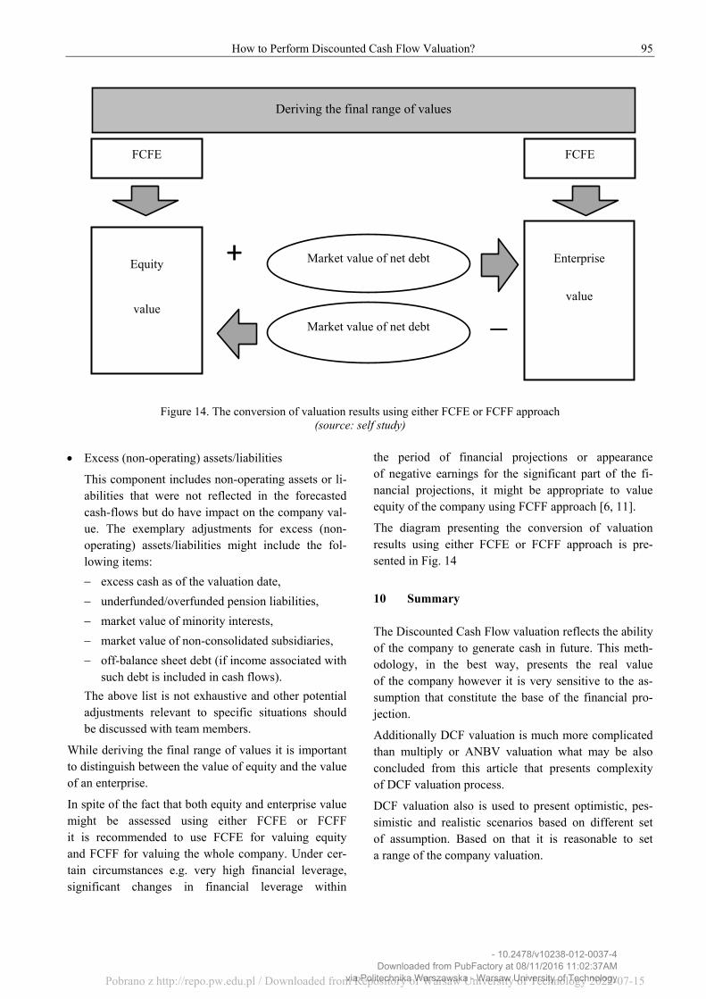
Figure 14. The conversion of valuation results using either FCFE or FCFF approach (source: self study)

Excess (non-operating) assets/liabilities

This component includes non-operating assets or li-abilities that were not reflected in the forecasted cash-flows but do have impact on the company val-ue. The exemplary adjustments for excess (non-operating) assets/liabilities might include the fol-lowing items:

excess cash as of the valuation date,

underfunded/overfunded pension liabilities,

market value of minority interests,

market value of non-consolidated subsidiaries,

off-balance sheet debt (if income associated with such debt is included in cash flows).

The above list is not exhaustive and other potential adjustments relevant to specific situations should be discussed with team members.

While deriving the final range of values it is important to distinguish between the value of equity and the value of an enterprise.

In spite of the fact that both equity and enterprise value might be assessed using either FCFE or FCFF it is recommended to use FCFE for valuing equity and FCFF for valuing the whole company. Under cer-tain circumstances e.g. very high financial leverage, significant changes in financial leverage within

the period of financial projections or appearance of negative earnings for the significant part of the fi-nancial projections, it might be appropriate to value equity of the company using FCFF approach [6, 11].

The diagram presenting the conversion of valuation results using either FCFE or FCFF approach is pre-sented in Fig. 14

10 Summary The Discounted Cash Flow valuation reflects the ability of the company to generate cash in future. This meth-odology, in the best way, presents the real value of the company however it is very sensitive to the as-sumption that constitute the base of the financial pro-jection.

Additionally DCF valuation is much more complicated than multiply or ANBV valuation what may be also concluded from this article that presents complexity of DCF valuation process.

DCF valuation also is used to present optimistic, pes-simistic and realistic scenarios based on different set of assumption. Based on that it is reasonable to set a range of the company valuation.

Deriving the final range of values

Equity

value

Enterprise

value

Market value of net debt

Market value of net debt

FCFE FCFE

+




11 References [1] Bösecke K. - Value Creation in Mergers, Acquisi-

tions and Alliances. Wiesbaden 2009.

[2] Copeland T., Koller T., Murrin J. - Valuation. Measuring and Managing the Value of Companies. John Wiley & Sons, New York 2000.

[3] Damodaran A. - Damodaran on Valuation: Security Analysis for Investment and Corporate Finance. Wiley Finance, 2006.

[4] Damodaran A. - Investment valuation. Tools and Techniques for Determining the Value of Any As-set. Sec. ed, John Wiley & Sons, Inc., New York 2002.

[5] Eccles R.G., Herz R.H., Keegan E.M., Phillips D.M.H. - The Value Reporting Revolution. Moving beyond the earnings gam. John Wiley & Sons, New York 2001.

[6] English J.R. - Applied Equity Analysis, Stock Valuation Techniques for Wall Street Profession-als. McGraw-Hill, New York 2001.

[7] Fernandez P. - Valuation Methods and Shareholder Value Creation. Academic Press, San Diego 2002.

[8] Frykman D., Tolleryd J. - Corporate valuation. Prentice Hall, London 2003.

[9] Keuleneer L., Verhoog W. - Recent Trends in Val-uation. John Wiley & Sons, The Atrium, Southern Gate, Chichester 2003.

[10] Pereiro L.E. - Valuation of Companies in Emerging Markets. John Wiley&Sons, New York 2002.

[11] Stowe J.D. - Equity asset valuation. John Wiley & Sons, Hoboken 2007.

[12] Szablewski A. - Wycena i zarządzanie wartością firmy, Wydawnictwo Poltext, Warszawa 2007.



how to perform discounted cash flow valuation? - repo pw

Documents