index policies for discounted bandit problems with availability constraints
TRANSCRIPT
INDEX POLICIES FOR DISCOUNTED BANDIT PROBLEMS WITHAVAILABILITY CONSTRAINTS
SAVAS DAYANIK, WARREN POWELL, AND KAZUTOSHI YAMAZAKI
Abstract. In the classical bandit problem, the arms of a slot machine are always available.
This paper studies the case where the arms are not always available. We first consider the
problem where the arms are intermittently available with some time-dependent probabilities.
We prove the non-existence of an optimal index policy and propose the so-called Whittle
index policy after reformulating the problem as a restless bandit. The index strikes the
balance between exploration and exploitation: it converges to the Gittins index as the
probability of availability approaches to one and to the immediate one-time reward as it
approaches to zero. We then consider the problem where the arms may break down and
repair is an option at some cost, and we derive the corresponding Whittle index policy.
We show that both problems are indexable and that the proposed index policies cannot
be dominated uniformly by any other index policy over the entire class of bandit problems
considered here. We illustrate how to evaluate one of the indices on a numerical example in
which rewards are Bernoulli random variables with unknown success probabilities.
1. Introduction
The multi-armed bandit problem considers the trade-off between exploration and exploita-
tion. It deals with the situations in which one needs to decide between actions that maximize
immediate reward and actions acquiring information that may help increase one’s total re-
ward in the future. In the classical multi-armed bandit problem, the decision maker has to
choose at each stage one arm of an N -armed slot machine to play in order to maximize his
expected total discounted reward over infinite time horizon. The reward obtained from an
arm depends on the state of a stochastic process that changes only when the arm is played.
Gittins and Jones [5] showed that each arm is associated with an index that is a function
of the state of the arm, and that the expected total discounted reward over infinite-horizon is
maximized if every time an arm with the largest index is played. We call an arm active if it
is played and passive otherwise. The proof (see, for example, Whittle [22] and Tsitsiklis [19])
relies on the condition that only active arms change their states. Due to this limitation, the
Date: May 20, 2007.
2000 Mathematics Subject Classification. Primary 93E20; Secondary 90B36.Key words and phrases. Optimal resource allocation, multi-armed bandit problems, Gittins index, Whittle
index, restart-in problem.1
2 SAVAS DAYANIK, WARREN POWELL, AND KAZUTOSHI YAMAZAKI
range of problems where optimal index policies are guaranteed to exist is small. Nevertheless,
the Gittins index policy is important because it considerably reduces the dimension of the
optimization problem by splitting it into N independent subproblems. Moreover, since at
each stage only one arm changes its state, at most one index has to be re-evaluated. For
this reason, many authors have generalized the classical multi-armed bandit problem and
studied performance of Gittins-like index policies for them.
In this paper, we study bandit problems where passive and active arms may become un-
available temporarily or permanently. Therefore, these are not classical multi-armed bandit
problems, and the Gittins index policies are not optimal any more.
For example in clinical trials, one chooses sequentially between alternative medicines to
prescribe to a number of patients. The arms correspond to medicines, and the state of
each arm corresponds to the state of knowledge about the corresponding medicine’s efficacy.
There are, however, situations where some medicine cannot be applied to certain patients.
For example, some medicines may go out of stock, or some patients are allergic to certain
ingredients of some medicines.
The bandit problems are also common in economics. In the face of the trade-off between
exploration and exploitation, rational decision makers are assumed to act optimally using
Gittins index policy. This framework has been used to explain, for example, insufficient
learning (Rothschild [18], Banks and Sundaram [1], and Brezzi and Lai [4]), matching and
job search (Jovanovic [10] and Miller [14]) and mechanism design (Bergemann and Valimaki
[3]). However, decision makers do not act in the same way when alternatives may become
unavailable in the future. Intuitively, the more pessimistic a decision maker is about the
future availability of the alternatives, the more focused he gets to immediate payoffs. There-
fore, it is questionable to expect that decision makers use the Gittins index policy in the
situations where the alternatives occasionally become unavailable.
In a variation of the above-mentioned problem, we assume that arms may break down,
and that the decision maker has the option to fix them. For example, if an energy company
loses the access to oil due to an unexpected international conflict, will it be worth the effort
to get another access to oil or will it be better to rely on other resources available to the
company such as natural gas or coal? Bandit problems with switching costs (see, for example,
Jun [11]) is a special case; arms break down immediately if they are not engaged, and if a
broken arm is engaged, then the switching cost is incurred to repair. According to Bank
and Sundaram [2], it is difficult to imagine an economic problem where the agent can switch
costlessly between alternatives. They also showed that an optimal index policy does not
exist in the presence of switching costs.
BANDIT PROBLEM WITH AVAILABILITY CONSTRAINTS 3
We generalize the classical multi-armed bandit problem as follows. There are N arms,
and each arm is available with some state-dependent probability. At each decision stage,
the decision maker chooses M arms to play simultaneously and collects rewards from each
arm. The reward from arm n depends on a stochastic process Xn = (Xn(t))t≥0, whose state
changes only when the arm is played. The process Xn may represent, for example, the state
of the knowledge about the reward obtainable from arm n.
At every iteration, only a subset of the arms are available. We denote by Yn(t) the
availability of arm n at time t; it is one if the arm is available at time t, and zero otherwise.
Unlike Xn, the stochastic process Yn changes even when the arm is not played. The objective
is to find a policy that chooses arms so as to maximize the expected total discounted reward
collected over infinite horizon. We study the following two problems:
Problem 1. Each arm is intermittently available. Its availability at time t is unobservable
before time t. The conditional probability that an arm is available at time t+ 1 given
(i) the state X(t) and its availability Y (t) of the arm, and
(ii) whether or not the arm is played at time t
is known at time t. An arm cannot be played when it is unavailable.
This problem will not be well-defined unless there are at least M available arms to play
at each stage. We can, however, let the decision maker pull less than M arms at a time by
introducing sufficient number of arms that are always available and always give zero reward.
Problem 2. Arms are subject to failure, and the decision maker has the option to repair a
broken arm. Whether or not an arm is played at time t, it may break down and may not be
available at time t+ 1 with some probability that depends on
(i) the state X(t) of the arm at time, and
(ii) whether or not the arm is played at time t.
If an arm is broken, then the decision maker has the option to repair it at some cost (or
negative reward) that depends on X(t). Repairing an arm is equivalent to playing the arm
when it is broken. If an arm is repaired at time t, then it will be available at time t+ 1 with
some conditional probability that depends only on the state X(t) of the arm at time t. On
the other hand, if it is not repaired, then the arm remains broken at time t+ 1.
We show that an optimal index policy does not exist for either problem. Nevertheless,
there exists a near-optimal index policy that cannot be dominated uniformly by any other
index policy over all instances of either problem. The index we propose is based on the
Whittle index proposed for the restless bandit problems. We evaluate the performance of
the index policy for each problem both analytically and numerically.
4 SAVAS DAYANIK, WARREN POWELL, AND KAZUTOSHI YAMAZAKI
The restless bandit problem was introduced by Whittle [23], and it is a generalization of
the classical bandit problem in three directions: (i) the states of passive arms may change,
(ii) rewards can be collected from passive arms, and (iii) M ≥ 1 arms can be played simul-
taneously. Therefore, Problems 1 and 2 fall in the class of restless bandit problems. These
problems are computationally intractable; Papadimitriou and Tsitsiklis [16] proved that they
are PSPACE-hard. As in a typical restless bandit problem, we assume that rewards can be
collected from passive arms and that more than one arm can be pulled simultaneously.
Whittle [23] introduced the so-called Whittle index to maximize long-term average reward
and characterized the index as a Lagrange multiplier for a relaxed conservation constraint,
which ensures that on average M arms are played at each stage. The Whittle index policy
makes sense if the problem is indexable. Weber and Weiss [20, 21] proved that under indexa-
bility, the Whittle index policy is asymptotically optimal as M and N tend to infinity while
M/N is constant. The verification of indexability is hard in general. Whittle [23] gave an
example of a unindexable problem. However, indexability can be verified, and Whittle index
policy can be developed analytically, for example, for the dual-speed restless bandit problem
[7] and the problem in [8] with improving active arms and deteriorating passive arms.
Glazebrook et al. [6] considered a problem in which passive arms are subject to permanent
failure. They modeled it as a restless bandit, showed its indexability, and developed the
Whittle index policy. Problems 1 and 2 are the generalizations of their problem in that a
broken arm is allowed to get back to the system, and that both passive and active arms may
break down. We prove that Problems 1 and 2 are indexable and derive the Whittle indices.
Glazebrook et al.’s [6] and Gittins’ indices turn out to be the special cases of those indices.
We also evaluate the Whittle index numerically. Like the Gittins index, the Whittle
indices for Problems 1 and 2 are also the solutions to suitable optimal stopping problems.
We generalize Katehakis and Veinott’s [12] restart-in formulation of Gittins index to Problem
1’s Whittle index. Problem 2’s Whittle index turns out to be similar to the Gittins index,
and we use the original restart-in problem to calculate the index for Problem 2.
In Section 2, we start by modeling Problems 1 and 2 as restless bandits. In Section 3,
we review Whittle index and indexability. In Sections 4 and 5, we verify the indexability
of Problems 1 and 2 and develop corresponding Whittle indices; we also prove the non-
existence of an optimal index policy. A generalization of the restart-in problem that is
used to calculate Problem 1’s Whittle index is discussed in Section 6. We then consider a
numerical example in which the reward process is a Bernoulli process with unknown success
probability, and we evaluate the index policy. The example is introduced in Section 7, and
the results for Problems 1 and 2 are given in Sections 8 and 9, respectively. Section 10
contains the concluding remarks.
BANDIT PROBLEM WITH AVAILABILITY CONSTRAINTS 5
2. Model
We first model a general restless bandit problem that subsumes Problems 1 and 2, and
then specialize to the latter ones in Sections 4 and 5, respectively.
Using the stochastic processes X and Y defined in the previous section, the state of arm n
at time t can be denoted by Sn(t) = (Xn(t), Yn(t)). We denote by S(t) = (S1(t), S2(t), . . . , SN(t))
the state at time t of the system consisting of N arms.
Suppose that Xn takes values in Xn, n = 1, . . . , N , and let Sn = Xn × {0, 1}. The process
(Xn(t), Yn(t)) is a controlled time-homogeneous Markov process with the control
an(t) =
{1, if arm n is played at time t,
0, otherwise.
Let a(t) = (a1(t), a2(t), . . . , aN(t)) denote the control action at time t ≥ 0.
For every 1 ≤ n ≤ N , the process (Xn(t))t∈≥0 evolves according to a one-step transition
probability matrix p(n) = (p(n)xx′)x,x′∈Xn , if arm n is available and is played, and does not
change otherwise; that is, for every x, x′ ∈ Xn,
P {Xn(t+ 1) = x′|Xn(t) = x, Yn(t) = y, an(t) = a} =
{p
(n)xx′ , if y = a = 1,
δxx′ , if y = 0 or a = 0,
where δxx′ equals one if x = x′ and zero otherwise. Hence, even if arm n is active, the process
Xn does not change if the arm is unavailable. In Problem 2, activating an unavailable arm is
equivalent to repairing it. In that case, the process Xn does not change; namely, repairing an
arm only changes its availability. In Problem 1, activating an unavailable arm is not allowed.
We denote the conditional probability that arm n is available at time t + 1, given Xn(t),
Yn(t), and an(t) by
θan(x, y) , P {Yn(t+ 1) = 1|Xn(t) = x, Yn(t) = y, an(t) = a} ,(1)
for every (x, y) ∈ Sn, a ∈ {0, 1}, t ≥ 0, and 1 ≤ n ≤ N . In other words, the random variable
Yn(t+ 1) has conditionally Bernoulli distribution with success probability θa(t)n (Xn(t), Yn(t))
given Xn(t) and Yn(t). For every x ∈ Xn and a, y ∈ {0, 1}, let
Ran(x, y) , expected reward collected from arm n when Xn(t) = x, Yn(t) = y, an(t) = a,
and as in the classical bandit problem, we assume that Ran(x, y) is bounded uniformly over
x ∈ X and y ∈ {0, 1}. Let 0 < γ < 1 be a given discount rate. Then the expected
discounted immediate reward at time t equals E[γt∑N
n=1Ran(t)n (Xn(t), Yn(t))
]. If ai(t) = 1
and Yi(t) = 1, then Xi(t) changes to Xi(t+1) according to p(i). If aj(t) = 0 or Yj(t) = 0, then
Xj(t + 1) = Xj(t). If ai(t) = 1, then Yi(t + 1) equals one with probability θ1i (Xi(t), Yi(t)),
6 SAVAS DAYANIK, WARREN POWELL, AND KAZUTOSHI YAMAZAKI
and zero with probability 1 − θ1i (Xi(t), Yi(t)). If aj(t) = 0, then Yj(t + 1) equals one with
probability θ0j (Xj(t), Yj(t)), and zero with probability 1− θ0
j (Xj(t), Yj(t)).
The stochastic process (X, Y ) = (X(t), Y (t))t≥0 is Markovian; therefore, we only need to
consider stationary policies π : S1 × . . . × SN 7→ A ,{a ∈ {0, 1}N : a1 + . . .+ aN = M
}.
Denote for every fixed ((x1, y1), . . . , (xN , yN)) ∈ S1 × . . .× SN , the value under a stationary
policy π by Jπ(((x1, y1), . . . , (xN , yN))), and it equals
Eπ
[∞∑
t=0
γt
N∑n=1
Ran(t)n (Xn(t), Yn(t))
∣∣∣∣∣Xn(0) = xn, Yn(0) = yn, n = 1, 2, . . . , N
],
where an(t) = π((X1(t), Y1(t)), . . . , (XN(t), YN(t))) for every t ≥ 0. A policy π∗ ∈ Π
is optimal if it maximizes Jπ(((x1, y1), . . . , (xN , yN))) over π ∈ Π for every initial state
((x1, y1), . . . , (xN , yN)) in S1 × . . .× SN .
3. The Whittle index and indexability
Let us fix an arm and denote its state (X(t), Y (t)) as in Section 2, and consider the
following auxiliary problem. At each time, the decision maker can either activate the arm
or leave it resting. Suppose the current state of the arm is (x, y). If the arm is activated,
then reward R1(x, y) is obtained. If it is rested, then a subsidy W ∈ R and the passive
reward R0(x, y) are obtained. The objective is to maximize the expected total discounted
reward. Whittle [22] called this problem as the “W -subsidy problem”, and it is a variant
of the retirement problem (see, for example, Ross [17, Chapter VII]). The so-called Whittle
index corresponds to the smallest value of W for which it is optimal to rest the arm. After
Whittle index is calculated for every arm, the Whittle index policy is to activate an arm with
the largest index. However, this policy makes sense only if any arm which is rested under
a subsidy W is also rested under any subsidy W ′ > W . Namely, the set of states at which
it is optimal to rest the arm increases monotonically as the value of subsidy W increases.
This property is called indexability. These concepts were originally introduced by Whittle
[23] in the average-reward case, and their counterparts in the discounted case are described
by other authors; see, e.g., Nino-Mora [15].
3.1. Definitions. Because the indexability and Whittle index are examined for each fixed
isolated arm, we omit the subscripts identifying the arm. In the restless bandit problem, a
passive arm may change its state and give a nonzero reward. We denote the state process of
the arm by the controlled Markov process S = (S(t))t≥0 on some state space S, the control
action at time t by a(t), its transition matrix by
pass′ = P{S(t+ 1) = s′|S(t) = s, a(t) = a}, s, s′ ∈ S, a ∈ {0, 1},
BANDIT PROBLEM WITH AVAILABILITY CONSTRAINTS 7
and the expected reward obtained from the arm under action a ∈ {0, 1} by Ra(s), s ∈ S.
The arm is said to be active if action a = 1 is taken and passive otherwise.
For every fixed W ∈ R, the value function of the W -subsidy problem satisfies
V (s,W ) = max{L1(s,W ), L0(s,W )
},(2)
where
L1(s,W ) = R1(s) + γ∑s′∈S
p1ss′V (s′,W ), L0(s,W ) = W +R0(s) + γ
∑s′∈S
p0ss′V (s′,W )
are the maximum expected total rewards if the first action is to activate or to rest the arm,
respectively. We let Π(W ) be the subset of S in which it is optimal to choose the passive
action when the passive subsidy is W . Namely,
Π(W ) ,{s ∈ S : L1(s,W ) ≤ L0(s,W )
}, W ∈ R.
If an arm is indexable and it is optimal to rest the arm when the value of subsidy is W , then
it is also optimal to rest the same arm whenever the value of subsidy is greater than W .
Definition 3.1 (Indexability). An arm is indexable if Π(W ) is increasing in W ; namely,
W1 > W2 =⇒ Π(W1) ⊇ Π(W2).(3)
Definition 3.2 (Whittle index). The Whittle index of an indexable arm equals
W (s) , inf{W ∈ R : s ∈ Π(W )} in every state s ∈ S.(4)
Under indexability, the Whittle index is the smallest value of W for which both the active
and passive actions are optimal.
Definition 3.3 (Whittle index policy). Suppose that the arms of a restless bandit problem
are indexable. The Whittle index policy plays M arms with the largest Whittle-indices.
The W -subsidy problem is a special instance of Problems 1 and 2. If an optimal index
policy exists for those problems, then it must also be optimal for W -subsidy problem. This
observation will imply the non-existence of an optimal index policy; see Sections 4.5 and 5.3.
4. The Whittle index for Problem 1
This section presents an index policy for Problem 1. We obtain the Whittle index for
Problem 1 by studying the W -subsidy problem and prove the non-existence of an optimal
index policy. We will see that the Whittle index policy is the unique optimal index policy for
the W -subsidy problem up to a monotone transformation. Because the W -subsidy problem
is a special case of Problem 1, if there exists an optimal index policy for Problem 1, then it
8 SAVAS DAYANIK, WARREN POWELL, AND KAZUTOSHI YAMAZAKI
must be a strict monotone transformation of the Whittle index policy. We prove the non-
existence of an optimal index policy by showing an example in which the Whittle index policy
is not optimal. We also show that there does not exist an index policy that is uniformly
better than our Whittle index policy over all instances of Problem 1.
If an arm is unavailable, then only passive action is available, and the following holds.
Condition 4.1. For every x ∈ X , we have
(x, 0) ∈ Π(W ), W ∈ R. (inf ∅ ≡ −∞)(5)
4.1. TheW -subsidy problem for Problem 1. Recall from Section 1 that S(t) = (X(t), Y (t))t≥0
is the state process of a potentially unavailable arm. If the current state is s = (x, y) for
some x ∈ X and y ∈ {0, 1}, then the probability that the arm is available at the next stage
is given by θ1(x, y) if the arm is active, and by θ0(x, y) if it is passive; see (1).
For fixed W ∈ R, let the value function for the corresponding W -subsidy problem be
V ((·, ·),W ) : X × {0, 1} 7→ R. As in (2), it satisfies the Bellman equation
V ((x, y),W ) = max{L1((x, y),W ), L0((x, y),W )}, x ∈ X , y ∈ {0, 1},
where
L1((x, y),W ) = R1(x, y) + γ∑x′∈X
pxx′[(1− θ1(x, y))V ((x′, 0),W ) + θ1(x, y)V ((x′, 1),W )
],
L0((x, y),W ) = W +R0(x, y) + γ[(
1− θ0(x, y))V ((x, 0),W ) + θ0(x, y)V ((x, 1),W )
].
Let P1,0 be the probability law induced by the policy that the arm is active whenever it is
available, and it is passive otherwise. Similarly, let P0,0 be the probability law induced when
the arm is always rested. That is, P1,0 {X(t+ 1) = x′, Y (t+ 1) = y′|X(t) = x, Y (t) = y} is pxx′[θ1(x, 1)
]y′ [1− θ1(x, 1)
]1−y′, y = 1
δxx′[θ0(x, 0)
]y′ [1− θ0(x, 0)
]1−y′, y = 0
,
and P0,0 {X(t+ 1) = x′, Y (t+ 1) = y′|X(t) = x, Y (t) = y} = δxx′ [θ0(x, y)]y′
[1− θ0(x, y)]1−y′
.
Let E1,0x,y[·] and E0,0
x,y[·] be the expectations with respect to P1,0 and P0,0, respectively, given
that X(0) = x and Y (0) = y.
Denote by ρ(x, y) the expected total discounted reward from a passive arm whose current
state is (x, y) ∈ X × {0, 1}; namely,
ρ(x, y) , E0,0x,y
[∞∑
t=0
γtR0(X(t), Y (t))
]= E0,0
x,y
[∞∑
t=0
γtR0(x, Y (t))
].(6)
BANDIT PROBLEM WITH AVAILABILITY CONSTRAINTS 9
Let (Ft)t≥0 be the filtration generated by (X(t))t≥0 and (Y (t))t≥0, and S be the set of all
almost-surely (a.s.) positive stopping times of (Ft)t≥0, and define
S , {τ ∈ S : Y (τ) = 1 a.s.}
as the set of positive stopping times at which the arm is available.
The following proposition states that there exists an optimal index policy for the W -
subsidy problem. This will be used to obtain the Whittle index and prove the non-existence
of an optimal index policy for Problem 1. All of the proofs are deferred to the appendix.
Proposition 4.1. In the W -subsidy problem, resting the arm is optimal at state (x, 1),
namely (x, 1) ∈ Π(W ), if and only if
W ≥ (1− γ) supτ∈S
E1,0x,1
[∑τ−1t=0 γ
tRY (t)(X(t), Y (t)) + γτρ(X(τ), Y (τ))]− ρ(x, 1)
1− E1,0x,1
[(1− γ)
∑τ−1t=1 γ
t1{Y (t)=0} + γτ] .(7)
4.2. Including passive rewards. The Whittle index and indexability of Problem 1 are
easy consequences of Proposition 4.1. Note that the right-hand side of (7) is the minimum
value of subsidy at which it is optimal to make the arm passive when the state of the arm is
(x, 1); therefore, it corresponds by definition to the Whittle index of the arm.
Proposition 4.2. For every x ∈ X and y ∈ {0, 1}, the arm is indexable with the index
(8) W (x, y) ,(1− γ) sup
τ∈S
E1,0x,1
[∑τ−1t=0 γ
tRY (t)(X(t), Y (t)) + γτρ(X(τ), Y (τ))]− ρ(x, 1)
1− E1,0x,1
[(1− γ)
∑τ−1t=1 γ
t1{Y (t)=0} + γτ] , if y = 1,
−∞, otherwise.
The index in (8) is the generalization of that of Glazebrook et al., [6], who studied a
problem where only passive arms may become unavailable, and once arms are unavailable,
they never become available. This is a special case of Problem 1 with the following condition.
Condition 4.2. For every x ∈ X , suppose that θ1(x, 1) = 1 and θ1(x, 0) = θ0(x, 0) = 0.
Corollary 4.1 (Glazebrook et al. [6, Theorem 2]). Suppose Conditions 4.1 and 4.2 hold.
Then the arm is indexable with the index W (x, y) defined for every x ∈ X by
(1− γ) sup
τ∈S
E1,0x,1
[∑τ−1t=0 γ
tR1(X(t), Y (t)) + γτρ(X(τ), Y (τ))]− ρ(x, 1)
1− E1,0x,1 [γτ ]
, if y = 1
−∞, otherwise
.
(9)
10 SAVAS DAYANIK, WARREN POWELL, AND KAZUTOSHI YAMAZAKI
4.3. The Whittle index if passive arms do not give rewards. We now derive the
Whittle index when passive arms do not give rewards. That is, in addition to Condition 4.1,
we also assume the following.
Condition 4.3. Suppose that R0(x, y) = 0 holds for every x ∈ X and y ∈ {0, 1}.
The arm is indeed indexable, and the Whittle index is given by the following corollary.
Corollary 4.2. If Conditions 4.1 and 4.3 hold, then the arm is indexable with the index
W (x, y) =
(1− γ) supτ∈S E1,0
x,1
[∑τ−1t=0 γ
tR1(X(t), Y (t))1{Y (t)=1}]
1− E1,0x,1
[∑τ−1t=1 (1− γ)γt1{Y (t)=0} + γτ
],
if y = 1
−∞, otherwise
, x ∈ X .
(10)
We omit the proof as the result is immediate from Proposition 4.2 after substituting
R0(x, y) = 0 for every x ∈ X and y ∈ {0, 1}. The index (10) can be simplified further when
the probability of availability does not depend on the state of X and Y .
Corollary 4.3. Suppose Conditions 4.1 and 4.3 hold, and θ0(x, y) = θ1(x, y) = θ ∈ [0, 1] is
constant for every x ∈ X and y ∈ {0, 1}. Then the arm is indexable with the index
W (x, y) =
(1− γ) supτ∈S E1,0
x,1
[∑τ−1t=0 γ
tR1(X(t), Y (t))1{Y (t)=1}]
1− γ(1− θ)− θE1,0x,1 [γτ ],
if y = 1
−∞, otherwise
, x ∈ X .
(11)
4.4. The convergence of the Whittle index to the Gittins index or to the immedi-
ate expected reward. We now analyze the Whittle index (11) as a function of probability
of availability θ ∈ [0, 1]. Firstly, the Whittle index is a generalization of the Gittins index:
they coincide when the arm is always available, as the next corollary shows; therefore, they
are optimal for the classical bandit problem.
Corollary 4.4. Suppose the arm is always available; i.e.,
θ0(x, y) = θ1(x, y) = 1, x ∈ X , y ∈ {0, 1}.(12)
Then the arm is indexable with the index
W (x, y) =
supτ∈S
E1,0x,1
[∑τ−1t=0 γ
tR1(X(t), Y (t))]
E1,0x,1
[∑τ−1t=0 γ
t] , if y = 1
−∞, otherwise
, x ∈ X .(13)
BANDIT PROBLEM WITH AVAILABILITY CONSTRAINTS 11
Since each arm is available with probability one, the probability law P1,0 chooses the active
action all the time. Thus, the Whittle index policy is optimal in the classical bandit problem.
Secondly, if θ0(x, y) = θ1(x, y) = 0 for every x ∈ X and y ∈ {0, 1}, then the index becomes
W (x, 1) = R1(x, 1), x ∈ X .(14)
The next proposition shows that the limits of the Whittle index in (11) as θ ↗ 1 and θ ↘ 0
exist and coincide with its extreme values in (13) and (14), respectively.
Proposition 4.3. The Whittle index W (x, 1) defined in (11) converges to the Gittins index
as θ ↗ 1, and to the one-time reward R1(x, 1) as θ ↘ 0 uniformly over x ∈ X .
The result is also intuitive. If the probability of availability is small, then the decision
maker becomes myopic; she does not care too much about the future rewards, because she
expects that the arm will not be available for most of the time. Consider, for example, the
situation in which there is one arm which is always available and gives her a constant reward
while the other arms are available today, but she knows that they will not be available in the
future. The optimal strategy is to pick today the arm with the highest immediate reward
and to pick tomorrow and in the future the only arm that is available. On the other hand,
as θ ↗ 1, the problem becomes more similar to the classical bandit problem, and the index
converges to the optimal Gittins index by Proposition 4.3.
4.5. The non-existence of an optimal policy. We conclude this section by proving the
non-existence of an optimal index policy for Problem 1. This is true even in a special case
in which M = 1, passive arms do not give rewards, and the probability of availability is
consistent. We claim that if there exists an optimal index policy, then it must be a strict
monotone transformation of the index defined by (8). We then show the non-existence of an
optimal index policy by showing an example in which the index policy is not optimal.
Proposition 4.4. Any index that is optimal for every instance of Problem 1 must be a strict
monotone transformation of the index W (·, ·) in (8).
Proposition 4.5. An optimal index policy does not exist for Problem 1.
If an optimal index policy exists for Problem 1, then it must be a strict monotone trans-
formation of (8) by Proposition 4.4. For, otherwise, it will not be optimal for the W -subsidy
problem, a special case of Problem 1. This also means that there does not exist an index
policy that uniformly dominates Whittle index policy over all of the instances of Problem 1.
12 SAVAS DAYANIK, WARREN POWELL, AND KAZUTOSHI YAMAZAKI
5. The Whittle index for Problem 2
Unlike in the previous problem, here we assume that the active action is still available
even when the arm is unavailable. Activating the arm is equivalent to repairing the arm.
We denote by Cn(x) > 0 the repair cost when arm n is broken at state x. If a broken arm
is not repaired, then it will be unavailable (or stay broken) the next time with probability
one. We assume that passive arms do not give rewards, and that the reward obtained from
activating an available arm is positive as in the following condition.
Condition 5.1. For every x ∈ X , y ∈ {0, 1}, and n = 1, . . . , N , suppose that R1n(x, 1) ≥ 0,
R1n(x, 0) = −Cn(x) < 0, R0
n(x, y) = 0, and θ0n(x, 0) = 0.
5.1. The W-subsidy problem and the Whittle index for Problem 2. As for Problem
1, we first consider the W -subsidy problem for Problem 2. Under Condition 5.1, the value
function of the W -subsidy problem satisfies
V ((x, y),W ) = max{L1((x, y),W ), L0((x, y),W )},
where for every x ∈ X , we have
L1((x, 1),W ) = R1(x, 1) + γ∑x′∈X
pxx′[(1− θ1(x, 1))V ((x′, 0),W ) + θ1(x, 1)V ((x′, 1),W )
],
L0((x, 1),W ) = W + γ[(1− θ0(x, 1))V ((x, 0),W ) + θ0(x, 1)V ((x, 1),W )
],
and
L1((x, 0),W ) = −C(x) + γ[(1− θ1(x, 0))V ((x, 0),W ) + θ1(x, 0)V ((x, 1),W )
],
L0((x, 0),W ) = W + γV ((x, 0),W ).
Similar to P1,0 and P0,0 of the previous section, let P1,1 be the probability law induced by
the policy that activates the arm forever and E1,1 denote the expectation with respect to
P1,1. Moreover, let ψ(x) be the expected total discounted reward if the arm is active forever
starting in state (x, 1) at time zero. Namely,
ψ(x) , E1,1x,1
[∞∑
t=0
γt{R1(X(t), Y (t))1{Y (t)=1} − C(X(t))1{Y (t)=0}
}].(15)
Condition 5.2. Suppose that we have ψ(x) ≥ −C(x)/(1− γ) for every x ∈ X .
Condition 5.2 is satisfied, for example, if
(i) the arm never breaks under the active action; i.e., θ1(x, 1) = 1 for every x ∈ X , or
(ii) C(X(t)) is constant or non-increasing almost surely under the active action.
BANDIT PROBLEM WITH AVAILABILITY CONSTRAINTS 13
Proposition 5.1. Under Condition 5.2, in the W -subsidy problem for Problem 2, activating
the arm is optimal if and only if
W ≥ (1− γ) supτ∈S
E1,1x,y
[∑τ−1t=0 γ
tR1(X(t), Y (t))]
1− E1,1x,y [γτ ]
.
Proposition 5.2. If Condition 5.2 holds, then the arm is indexable with the index
W (x, y) = (1− γ) supτ∈S
E1,1x,y
[∑τ−1t=0 γ
tR1(X(t), Y (t))]
1− E1,1x,y [γτ ]
, x ∈ X , y ∈ {0, 1}.(16)
Remark 5.1. If Condition 4.2 holds, then the problem reduces to a problem studied by
Glazebrook et al. [6] where passive arms do not give rewards, and the indices coincide.
5.2. The connection to the bandit problems with switching costs. The problem is
reduced to the classical bandit problem with switching costs if θ1(x, 1) = 1, and if Cn(x) is
the cost of switching to arm n when the current state of arm n is x. Condition 5.2 holds
because θ1(x, 1) = 1; therefore, the Whittle index is indexable. Glazebrook et al. [9] have
formulated the problem as a restless bandit problem. Their formulation is slightly different
from ours in that one does not have to wait for the arm to be fixed; when one plays a broken
arm, he obtains its immediate reward minus the switching cost and the arm is guaranteed to
be available the next time. Nevertheless, the form of their index is the same as ours. They
showed numerically that their index policy is nearly optimal.
5.3. The non-existence of an optimal policy. As in Problem 1, an optimal index policy
does not exist for Problem 2. We again show that if there exists one, then the corresponding
index must be a strict monotone transformation of our index, and we give an example where
our index policy is not optimal. Proof of Proposition 5.3 is omitted because it is very similar
to that of Proposition 4.4.
Proposition 5.3. If there is an optimal index policy for Problem 2, then the index must be
a strict monotone transformation of the index W (·, ·) in (16).
Proposition 5.4. An optimal index policy does not exist for Problem 2.
6. The restart-in problem
We have developed the Whittle indices for Problems 1 and 2 in the previous sections.
Here we assume that passive arms do not give rewards and discuss how to compute the
indices in (10) and (16). To this end, we develop the restart-in problem representation of the
indices. The restart-in problem representation of the Gittins index for the classical multi-
armed bandit problem was introduced by Katehakis and Veinott [13]. The index in (16) is
14 SAVAS DAYANIK, WARREN POWELL, AND KAZUTOSHI YAMAZAKI
similar to the Gittins index; therefore, we first formulate it as a restart-in problem. We then
propose a generalization of restart-in problem representation for the Whittle index in (10).
6.1. The restart-in problem for the Gittins index. We first review the restart-in prob-
lem formulated by Katehakis and Veinott [13]. Consider the classical multi-armed bandit
problem where a fixed arm follows a stochastic process S = (S(t))t≥0 on some state space Sand evolves according to a transition matrix p = (pss′)ss′∈S under the active action, and let
R(s) be the one-time reward obtained when the state of the arm is s and when it is active.
Katehakis and Veinott [13] showed that the Gittins index of the arm at state s ∈ S equals
(1− γ)νs, where ν = (νs)s∈S satisfies the optimality equation
νs = max
(R(s) + γ
∑s′∈S
pss′νs′ , R(s) + γ∑s′∈S
pss′νs′
), s ∈ S;(17)
particularly,
νs = supτ>0
E[∑τ−1
t=0 γtR(S(t))
∣∣S(0) = s]
E [1− γτ ]= sup
τ>0
E[∑τ−1
t=0 γtR(S(t))
∣∣S(0) = s]
(1− γ)E[∑τ−1
t=0 γt] .
The Gittins index at a fixed state s is the solution of |S| equations defined by (17), and it
can be calculated by the value-iteration algorithm applied to (17).
We now characterize the Whittle indices in (5.2) and (10) of a potentially unavailable arm
as the value function of a restart-in problem.
6.2. The restart-in problem representation of (16). Because (16) and Gittins index
are similar, we can use the restart-in problem representation of the Gittins index, after we
multiply each one-time reward by (1− γ). Namely, W (x, y) equals νx,y if R1(x, 0) = −C(x)
and (νx,y)x∈X ,y∈{0,1} satisfies for every x ∈ X and y ∈ {0, 1},
(18) νx,y = max
((1− γ)R1(x, y) + γ
∑x′∈X
pxx′[θ1(x, y)νx′,1 + (1− θ1(x, y))νx′,0
],
(1− γ)R1(x, y) + γ∑x′∈X
pxx′[θ1(x, y)νx′,1 + (1− θ1(x, y))νx′,0
]).
6.3. The restart-in problem representation for (10). Fix x ∈ X and define (νx,y)x∈X ,y∈{0,1}
such that, for every x ∈ X ,
(19) νx,1 = max
((1− γ)R1(x, 1) + γ
∑x′∈X
pxx′[θ1(x, 1)νx′,1 + (1− θ1(x, 1))νx′,0
],
(1− γ)R1(x, 1) + γ∑x′∈X
pxx′[θ1(x, 1)νx′,1 + (1− θ1(x, 1))νx′,0
]),
BANDIT PROBLEM WITH AVAILABILITY CONSTRAINTS 15
and
νx,0 = (1− γ)νx,1 + γ(θ0(x, 0)νx,1 + (1− θ0(x, 0))νx,0
).(20)
Next proposition shows that if (νx,y)x∈X ,y∈{0,1} satisfies (19) and (20), then νx,1 coincides
with the index in (2) of the arm in state (x, 1).
Proposition 6.1. If (νx,y)x∈X ,y∈{0,1} satisfies (19) and (20), then we have
νx,1 = (1− γ) supτ∈S
E1,0x,1
[∑τ−1t=0 γ
tR1(X(t), Y (t))1{Y (t)=1}]
1− E1,0x,1
[∑τ−1t=1 (1− γ)γt1{Y (t)=0} + γτ
] .(21)
Remark 6.1. Suppose θ1(x, 1) = 1 for every x ∈ X as in the classical multi-armed bandit
problem. Then (19) becomes
νx,1 = max
{(1− γ)R1(x, 1) + γ
∑x′∈X
pxx′νx′,1, (1− γ)R1(x, 1) + γ∑x′∈X
pxx′νx′,1
},
which is Katehakis and Veinott’s [13] restart-in problem representation of the Gittins index
after multiplication by (1−γ). Indeed, νx,1 equals the Gittins index of the arm in state (x, 1).
7. An example
We will illustrate how to evaluate Whittle indices in (10) and (16) and compare Whittle
and other index policies for Problems 1 and 2, in which the reward of each arm is a Bernoulli
random variable with some unknown success probability. The success probability of arm n
is a random variable λn having beta distribution with parameters an and bn; namely,
P {λn ∈ dr} =Γ(an + bn)
Γ(an)Γ(bn)ran−1(1− r)bn−1dr,
and let Cn > 0 be the repair cost for arm n in Problem 2.
Katehakis and Derman [12] approximate the Gittins index for the classical two-armed
bandit problem with Bernoulli distributed rewards. We generalize their approximation to
calculate the Whittle indices in (10) and (16). In the next section, we compute the Whittle
indices and evaluate corresponding index policies. Here we shall omit the subscripts that
identify the arms, because we compute the index for each arm separately.
If the parameters of the current beta distribution of λ are (a, b), and if c successes and d
failures are observed after c+ d plays, then the posterior probability distribution of λ is also
beta with parameters (a+ c, b+ d).
Let X(t) denote the parameters of the posterior beta distribution of λ after t plays. Then
the pair (X,Y ) stores all of the information needed; it is a Markov process that evolves
16 SAVAS DAYANIK, WARREN POWELL, AND KAZUTOSHI YAMAZAKI
under the active action according to transition probabilities
p(a,b),(a+1,b) =a
a+ b, p(a,b),(a,b+1) =
b
a+ b.
The one-time expected reward given X(t) = (a, b) and Y (t) = 1 at time t is a/(a + b).
We formulate the restart-in problem representation for Problems 1 and 2 and describe a
computational method analogous to that of Katehakis and Derman [12].
7.1. The restart-in problem for Problem 1. Specializing (19) and (20), the Whittle
index of the arm in state (x, 1) = ((a, b), 1) is given by W ((a, b), 1) = ν(a,b),1, which satisfy
ν(a,b),1 = max(L(a, b),L(a, b)),(22)
ν(a,b),0 = (1− γ)ν(a,b),1 + γ[θ0((a, b), 0)ν(a,b),1 + (1− θ0((a, b), 0))ν(a,b),0
],(23)
for every (a, b) ∈ N2, where
L(a, b) = (1− γ)R1((a, b), 1) + γ[θ1((a, b), 1)
(p(a,b)(a+1,b)ν(a+1,b),1 + p(a,b)(a,b+1)ν(a,b+1),1
)+(1− θ1((a, b), 1))
(p(a,b)(a+1,b)ν(a+1,b),0 + p(a,b)(a,b+1)ν(a,b+1),0
)]= (1− γ)
a
a+ b+ γ
[θ1((a, b), 1)
(a
a+ bν(a+1,b),1 +
b
a+ bν(a,b+1),1
)+(1− θ1((a, b), 1))
(a
a+ bν(a+1,b),0 +
b
a+ bν(a,b+1),0
)].
7.2. The restart-in problem for Problem 2. The Whittle index of the arm at state
(x, y) = ((a, b), y) is given by W ((a, b), y) = ν(a,b),y, which satisfy
ν(a,b),y = max(L((a, b), y),L((a, b), y))(24)
for every (a, b) ∈ N2 and y ∈ {0, 1}, where L((a, b), y) equals
(1− γ)R1((a, b), y) + γ[θ1((a, b), y)
(p(a,b)(a+1,b)ν(a+1,b),1 + p(a,b)(a,b+1)ν(a,b+1),1
)+(1− θ1((a, b), y)
(p(a,b)(a+1,b)ν(a+1,b),0 + p(a,b)(a,b+1)ν(k,l+1),0
)]= (1− γ)
(a
a+ b1{1}(y)− C1{0}(y)
)+ γ
[θ1((a, b), y)
(a
a+ bν(a+1,b),1 +
b
a+ bν(a,b+1),1
)+(1− θ1((a, b), y)
(a
a+ bν(a+1,b),0 +
b
a+ bν(a,b+1),0
)].
7.3. Computing the Whittle indices. We can calculate the Whittle indices (10) and (16)
by solving, with the value iteration algorithm, the Bellman equations (22), (23), and (24),
respectively. Katehakis and Derman [12] calculated the Gittins index for a classical bandit
problem with two Bernoulli arms after truncating the state space of the process X to
ZL ={(a, b) ∈ N2 : a+ b ≤ L
}(25)
BANDIT PROBLEM WITH AVAILABILITY CONSTRAINTS 17
for some fixed integer L > 0. In the same manner, we only consider states s = (x, y) where
x = (a, b) ∈ ZL and y ∈ {0, 1}. Katehakis and Derman [12] proved that as L increases, their
approximation converges to the true value of the Gittins index. It is easy to prove that the
same result holds in our settings.
7.4. Some bounds on the optimal value function of the restart-in problem. We dis-
cuss how to obtain some upper and lower bounds on the optimal value function. In principle,
the optimal values can be computed by solving the dynamic programming equations using,
for example, the value iteration algorithm. In practice, however, they are computationally
intractable when the number of arms is large.
Let J∗(s) denote the optimal value when the state of arm n is sn = ((an, bn), yn) for
n = 1, . . . , N . Let j and j be some upper and lower bounds of J∗, respectively. Namely,
j(s) ≤ J∗(s) ≤ j(s), s ∈ S1 × . . .× SN .
We truncate the state space to (ZL × {0, 1})N , where ZL is defined as in (25).
Now we can replace the reward at the boundaries by their bounds and use backward
induction to obtain bounds on the value function on the entire truncated state space. For
s ∈ (ZL × {0, 1})N , define J(s) = j(s) and J(s) = j(s) where ZL = {(a, b) ∈ N2 : a+b = L},and calculate J(s) and J(s) by solving the same Bellman equation for J∗(·). By monotonicity,
J(s) ≤ J∗(s) ≤ J(s), s ∈ (ZL × {0, 1})N .
8. Numerical results for Problem 1
We provide numerical results obtained for Problem 1 in this section. We considered the
problem where the reward process is defined as in Section 7, and the probability that an arm
is available is constant. The corresponding Whittle index is given by (11).
8.1. Computing the Whittle indices. We computed the Whittle indices for probabilities
of availability θ = 0.1, 0.3, 0.5, 0.7, 0.9, 1.0 and γ = 0.9 using the algorithm described in the
previous section with L = 200. These indices are tabulated in Appendix B. Recall that the
Whittle index is a generalization of the Gittins index and coincides with the Gittins index
when θ = 1. Indeed, we obtained the same values as Katehakis and Derman [13] for θ = 1
after multiplying by (1 − γ). Moreover, as the value of θ decreases to 0, as we proved in
Proposition 4.3, the index converges to the one-time reward. Note that the indices are very
close to the one-time reward a/(a+ b) when θ = 0.1.
18 SAVAS DAYANIK, WARREN POWELL, AND KAZUTOSHI YAMAZAKI
θ1 θ2 θ3 lower/upper bounds Whittle (95 % CI) Gittins (95 % CI)
1.0 1.0 1.0 (6.49292, 6.60618) 6.5426 (6.5381, 6.5471) 6.5426 (6.5381, 6.5471)
0.7 0.7 1.0 (6.17190, 6.22723) 6.1782 (6.1737, 6.1827) 6.1673 (6.1630, 6.1716)
0.7 0.5 1.0 (6.04527, 6.09630) 6.0304 (6.0259, 6.0349) 6.0357 (6.0314, 6.0400)
0.7 0.3 1.0 (5.92097, 5.97950) 5.9295 (5.9248, 5.9342) 5.9076 (5.9033, 5.9119)
0.7 0.1 1.0 (5.81247, 5.88546) 5.8155 (5.8106, 5.8204) 5.7866 (5.7821, 5.7911)
0.5 0.5 1.0 (5.89183, 5.93610) 5.8942 (5.8897, 5.8987) 5.8826 (5.8783, 5.8869)
0.5 0.3 1.0 (5.74100, 5.79254) 5.7308 (5.7261, 5.7355) 5.7293 (5.7248, 5.7338)
0.5 0.1 1.0 (5.60574, 5.67005) 5.5987 (5.5938, 5.6036) 5.5868 (5.5821, 5.5915)
0.3 0.3 1.0 (5.55919, 5.62343) 5.5503 (5.5454, 5.5552) 5.5562 (5.5517, 5.5607)
0.3 0.1 1.0 (5.39082, 5.39082) 5.3924 (5.3871, 5.3977) 5.3864 (5.3815, 5.3913)
0.1 0.1 1.0 (5.18692, 5.31909) 5.1898 (5.1843, 5.1953) 5.1888 (5.1837, 5.1939)
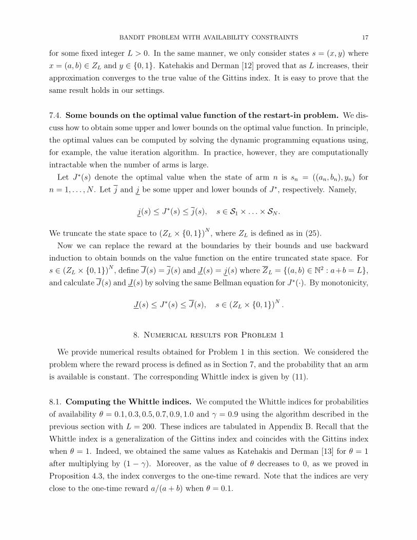
Table 1. The comparison of the optimal policy and the Whittle and Gittins
index policies
8.2. Evaluation of the Whittle index policy. We start by comparing the Whittle index
policy and the optimal policy. Suppose that there are exactly three arms. Arms 1 and 2 are
available with some fixed probability θ ∈ [0, 1], and arm 3 is available with probability one.
With larger number of arms, an interesting and hopefully tight lower bound of the optimal
value can be obtained by applying the Gittins index. Analogous to the Whittle index policy,
we define the Gittins index policy
Definition 8.1 (Gittins index policy). The Gittins index policy chooses, by definition, the
arm with the largest Gittins index among the available arms. The Gittins index coincides
with the Whittle index when θ = 1.
When the number of arms is more than three, we compared the Whittle index policy with
the Gittins index policy. We have tested several cases in which M out of N arms are played
each time. The parameters of the initial beta distribution of the reward from each arm is
(a, b) = (1, 1), and there are always M arms with θ = 1. In case of a tie, we pick a random
subset of M arms with the largest indices.
8.3. Results. Table 1 compares the upper and lower bounds on the optimal expected total
discounted reward values and expected total discounted rewards obtained by applying the
Whittle and Gittins index policies when the number of arms is three. The bounds on the
optimal values were obtained by the backward induction algorithm as described in Section
7.4 with j(s) =∑∞
t=0 γt1 = 1/(1 − γ), and j(s) = a3/(a3 + b3). Here, j(s) ≥ J∗(s) because
one-time reward is bounded from above by one, and j(s) ≤ J∗(s) because j(s) can be
BANDIT PROBLEM WITH AVAILABILITY CONSTRAINTS 19
10 15 20 25 30
5.0
5.5
6.0
6.5
7.0
7.5
L
Rew
ard
unde
r W
hittl
e in
dex
polic
y an
d bo
unds
● ● ● ● ● ● ● ● ● ● ● ● ● ● ● ● ● ● ● ● ● ● ● ●
10 15 20 25 30
5.0
5.5
6.0
6.5
7.0
7.5
L
Rew
ard
unde
r W
hittl
e in
dex
polic
y an
d bo
unds
● ● ● ● ● ● ● ● ● ● ● ● ● ● ● ● ● ● ● ● ● ● ● ●
(a) θ1 = 0.7, θ2 = 0.7, θ3 = 1.0 (b) θ1 = 0.5, θ2 = 0.5, θ3 = 1.0
10 15 20 25 30
5.0
5.5
6.0
6.5
7.0
7.5
L
Rew
ard
unde
r W
hittl
e in
dex
polic
y an
d bo
unds
● ● ● ● ● ● ● ● ● ● ● ● ● ● ● ● ● ● ● ● ● ● ● ●
10 15 20 25 305.
05.
56.
06.
57.
07.
5
L
Rew
ard
unde
r W
hittl
e in
dex
polic
y an
d bo
unds
● ● ● ● ● ● ● ● ● ● ● ● ● ● ● ● ● ● ● ● ● ● ● ●
(c) θ1 = 0.3, θ2 = 0.3, θ3 = 1.0 (d) θ1 = 0.1, θ2 = 0.1, θ3 = 1.0
10 15 20 25 30
5.0
5.5
6.0
6.5
7.0
7.5
L
Rew
ard
unde
r W
hittl
e in
dex
polic
y an
d bo
unds
● ● ● ● ● ● ● ● ● ● ● ● ● ● ● ● ● ● ● ● ● ● ● ●
10 15 20 25 30
5.0
5.5
6.0
6.5
7.0
7.5
L
Rew
ard
unde
r W
hittl
e in
dex
polic
y an
d bo
unds
● ● ● ● ● ● ● ● ● ● ● ● ● ● ● ● ● ● ● ● ● ● ● ●
(e) θ1 = 0.7, θ2 = 0.3, θ3 = 1.0 (f) θ1 = 0.5, θ2 = 0.1, θ3 = 1.0
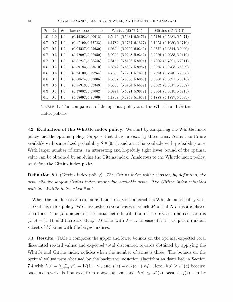
Figure 1. The upper/lower bounds on the optimal expected total discounted
reward and expected total discounted reward under the Whittle index policy
as a function of L at state (X1, Y1) = (X2, Y2) = (X3, Y3) = ((1, 1), 1).
attained by pulling arm 3, which is always available. The values under the Whittle and
Gittins index policies are calculated by Monte Carlo simulation based on 1,000,000 samples.
Figure 1 shows the upper and lower bounds and the value under the Whittle index policy
as a function of L used in the definition of the truncated space ZL in (25). The bounds
converge to the optimal value as L increases, and we can see how close the value obtained
by the Whittle index policy is to the optimal value.
20 SAVAS DAYANIK, WARREN POWELL, AND KAZUTOSHI YAMAZAKI
N M Whittle (95% CI) Gittins (95% CI) M Whittle (95% CI) Gittins (95% CI)
Case 1:
2 1 5.5474 (5.5313, 5.5635) 5.5587 (5.543, 5.5744)
6 1 6.6181 (6.6056, 6.6306) 6.4784 (6.4672, 6.4896)
12 1 6.9357 (6.9245, 6.9464) 6.5600 (6.5502, 6.5698) 2 13.7052 (13.6885, 13.7219) 13.3439 (13.3288, 13.3590)
18 1 7.0225 (7.0119, 7.0331) 6.6442 (6.6342, 6.6542) 3 20.6722 (20.6518, 60.6926) 20.1230 (20.1052, 20.1408)
24 1 7.0307 (7.0202, 7.0410) 6.6391 (6.6291, 6.6491) 4 27.6446 (27.6213, 27.6679) 26.8526 (26.8526, 26.8934)
30 1 7.0301 (7.0197, 7.0405) 6.6459 (6.6359, 6.6559) 5 34.6193 (34.5934, 34.6452) 33.6254 (33.6027, 33.6481)
36 1 7.0297 (7.0193, 7.0401) 6.6346 (6.6246, 6.6446) 6 41.5967 (41.5687, 41.6254) 40.3890 (40.3643, 40.4137)
Case 2:
3 1 5.9132 (5.8985, 5.9279) 5.9255 (5.9116, 5.9394)
6 1 6.6227 (6.6102, 6.6352) 6.4724 (6.4612, 6.4836)
12 1 6.9309 (6.9199, 6.9419) 6.5544 (6.5446, 6.5642) 2 13.5260 (13.5088, 13.5432) 13.1447 (13.1298, 13.1596)
18 1 6.9930 (6.9824, 7.0036) 6.5223 (6.5127, 6.5319) 3 20.4339 (20.4129, 20.4549) 19.7741 (19.7563, 19.7919)
24 1 7.0178 (7.0072, 7.0284) 6.4806 (6.4708, 6.4904) 4 27.3402 (27.3163, 27.3641) 26.4494 (26.4290, 26.4698)
30 1 7.0214 (7.0110, 7.0318) 6.4530 (6.4432, 6.4628) 5 34.2210 (34.1943, 34.2477) 33.0992 (33.0765, 33.1219)
36 1 7.0266 (7.0162, 7.037) 6.4499 (6.4401, 6.4597) 6 41.1573 (41.1283, 41.1863) 39.7806 (39.7561, 39.8051)
Case 3:
6 1 6.5085 (6.4958, 6.5212) 6.3575 (6.3459, 6.3691)
12 1 6.8716 (6.8604, 6.8828) 6.5676 (6.5574, 6.5778) 2 13.3253 (13.3079, 13.3427) 12.9986 (12.9829, 13.0143)
18 1 6.9434 (6.9326, 6.9542) 6.5944 (6.5842, 6.6046) 3 20.1669 (20.1457, 20.1881) 19.6288 (19.6098, 19.6478)
24 1 6.9805 (6.9699, 6.9911) 6.6165 (6.6065, 6.6265) 4 27.0206 (26.9963, 27.0449) 26.2567 (26.2350, 26.2786)
30 1 7.0076 (6.9970, 7.0182) 6.6249 (6.6149, 6.6349) 5 33.8775 (33.8504, 33.9044) 32.8960 (32.8717, 32.9203)
36 1 7.0178 (7.0071, 7.0283) 6.6399 (6.6299, 6.6499) 6 40.7183 (40.6842, 40.7434) 39.5345 (39.5079, 39.5609)
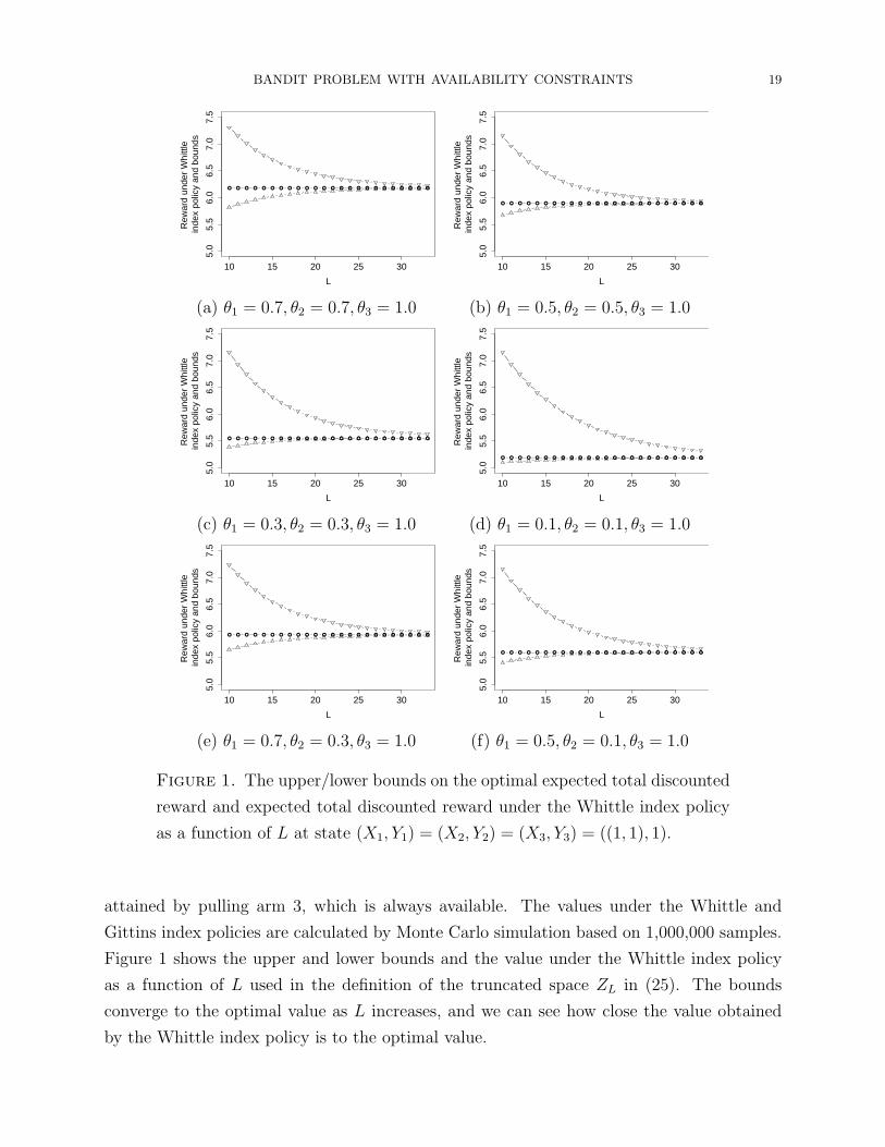
Table 2. The comparison of the expected total discounted rewards under
Whittle and Gittins index policies.
For larger number of arms, we compared the Whittle and Gittins index policies in the
following three cases, where M out of N arms are played every time; the results are shown
in Table 2.
case 1: N/2 arms are available with probability θ = 1.0 and 0.5,
case 2: N/3 arms are available with probability θ = 1.0, 0.7, and 0.3,
case 3: N/6 arms are available with probability θ = 1.0, 0.9, 0.7, 0.5, 0.3, and 0.1.
As seen from Table 1 and Figure 1, both the Whittle and Gittins index policies are as good
as the optimal policy, at least when the number of arms is small.
The Whittle index policy outperforms the Gittins index policy in most of the examples.
The Gittins index policy does not utilize the likelihood of each arm’s future availability, but
the Whittle index takes that information into account, and therefore it does better than the
Gittins index policy. Nevertheless, the Gittins index policy should give tight lower bounds
considering that the policy is optimal when each arm is always available.
BANDIT PROBLEM WITH AVAILABILITY CONSTRAINTS 21
N M optimal values (95% CI)
1 1 5.0021 (4.9962, 5.0080)
2 1 6.0963 (6.0912, 6.1014)
5 1 6.8722 (6.8602, 6.8842)
20 1 7.0151 (7.0045, 7.0257)
40 1 7.0261 (7.0156, 7.0364)
80 1 7.0256 (7.0152, 7.0360)
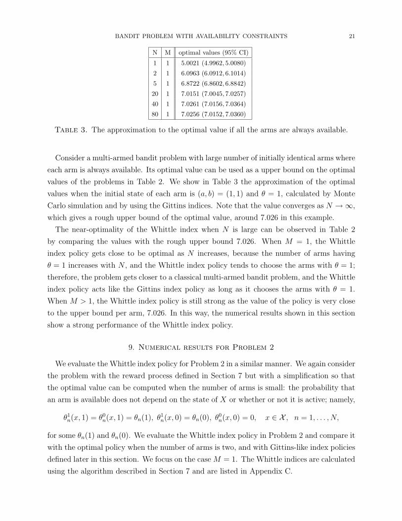
Table 3. The approximation to the optimal value if all the arms are always available.
Consider a multi-armed bandit problem with large number of initially identical arms where
each arm is always available. Its optimal value can be used as a upper bound on the optimal
values of the problems in Table 2. We show in Table 3 the approximation of the optimal
values when the initial state of each arm is (a, b) = (1, 1) and θ = 1, calculated by Monte
Carlo simulation and by using the Gittins indices. Note that the value converges as N →∞,
which gives a rough upper bound of the optimal value, around 7.026 in this example.
The near-optimality of the Whittle index when N is large can be observed in Table 2
by comparing the values with the rough upper bound 7.026. When M = 1, the Whittle
index policy gets close to be optimal as N increases, because the number of arms having
θ = 1 increases with N , and the Whittle index policy tends to choose the arms with θ = 1;
therefore, the problem gets closer to a classical multi-armed bandit problem, and the Whittle
index policy acts like the Gittins index policy as long as it chooses the arms with θ = 1.
When M > 1, the Whittle index policy is still strong as the value of the policy is very close
to the upper bound per arm, 7.026. In this way, the numerical results shown in this section
show a strong performance of the Whittle index policy.
9. Numerical results for Problem 2
We evaluate the Whittle index policy for Problem 2 in a similar manner. We again consider
the problem with the reward process defined in Section 7 but with a simplification so that
the optimal value can be computed when the number of arms is small: the probability that
an arm is available does not depend on the state of X or whether or not it is active; namely,
θ1n(x, 1) = θ0
n(x, 1) = θn(1), θ1n(x, 0) = θn(0), θ0
n(x, 0) = 0, x ∈ X , n = 1, . . . , N,
for some θn(1) and θn(0). We evaluate the Whittle index policy in Problem 2 and compare it
with the optimal policy when the number of arms is two, and with Gittins-like index policies
defined later in this section. We focus on the case M = 1. The Whittle indices are calculated
using the algorithm described in Section 7 and are listed in Appendix C.
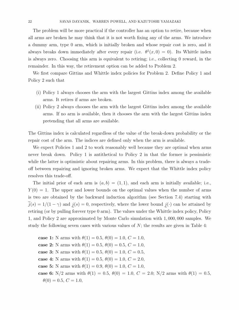
22 SAVAS DAYANIK, WARREN POWELL, AND KAZUTOSHI YAMAZAKI
The problem will be more practical if the controller has an option to retire, because when
all arms are broken he may think that it is not worth fixing any of the arms. We introduce
a dummy arm, type 0 arm, which is initially broken and whose repair cost is zero, and it
always breaks down immediately after every repair (i.e. θ1(x, 0) = 0). Its Whittle index
is always zero. Choosing this arm is equivalent to retiring; i.e., collecting 0 reward, in the
remainder. In this way, the retirement option can be added to Problem 2.
We first compare Gittins and Whittle index policies for Problem 2. Define Policy 1 and
Policy 2 such that
(i) Policy 1 always chooses the arm with the largest Gittins index among the available
arms. It retires if arms are broken.
(ii) Policy 2 always chooses the arm with the largest Gittins index among the available
arms. If no arm is available, then it chooses the arm with the largest Gittins index
pretending that all arms are available.
The Gittins index is calculated regardless of the value of the break-down probability or the
repair cost of the arm. The indices are defined only when the arm is available.
We expect Policies 1 and 2 to work reasonably well because they are optimal when arms
never break down. Policy 1 is antithetical to Policy 2 in that the former is pessimistic
while the latter is optimistic about repairing arms. In this problem, there is always a trade-
off between repairing and ignoring broken arms. We expect that the Whittle index policy
resolves this trade-off.
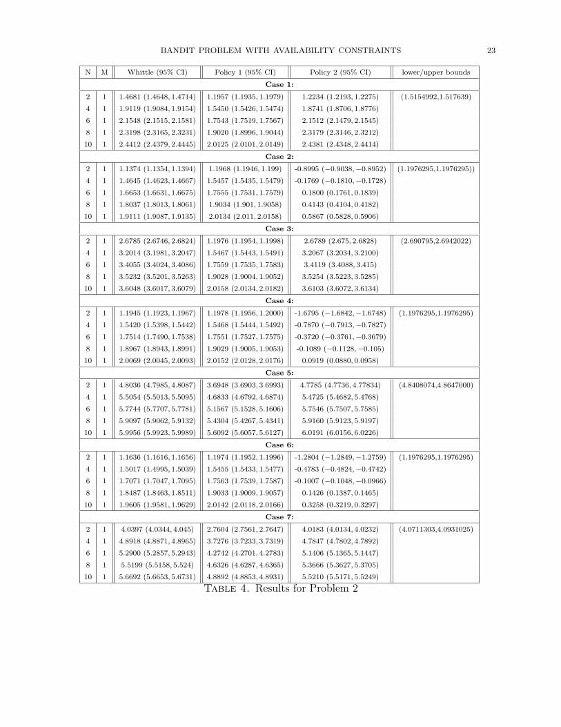
The initial prior of each arm is (a, b) = (1, 1), and each arm is initially available; i.e.,
Y (0) = 1. The upper and lower bounds on the optimal values when the number of arms
is two are obtained by the backward induction algorithm (see Section 7.4) starting with
j(s) = 1/(1− γ) and j(s) = 0, respectively, where the lower bound j(·) can be attained by
retiring (or by pulling forever type 0 arm). The values under the Whittle index policy, Policy
1, and Policy 2 are approximated by Monte Carlo simulation with 1, 000, 000 samples. We
study the following seven cases with various values of N ; the results are given in Table 4:
case 1: N arms with θ(1) = 0.5, θ(0) = 1.0, C = 1.0,
case 2: N arms with θ(1) = 0.5, θ(0) = 0.5, C = 1.0,
case 3: N arms with θ(1) = 0.5, θ(0) = 1.0, C = 0.5,
case 4: N arms with θ(1) = 0.5, θ(0) = 1.0, C = 2.0,
case 5: N arms with θ(1) = 0.9, θ(0) = 1.0, C = 1.0,
case 6: N/2 arms with θ(1) = 0.5, θ(0) = 1.0, C = 2.0; N/2 arms with θ(1) = 0.5,
θ(0) = 0.5, C = 1.0,
BANDIT PROBLEM WITH AVAILABILITY CONSTRAINTS 23
N M Whittle (95% CI) Policy 1 (95% CI) Policy 2 (95% CI) lower/upper bounds
Case 1:
2 1 1.4681 (1.4648, 1.4714) 1.1957 (1.1935, 1.1979) 1.2234 (1.2193, 1.2275) (1.5154992,1.517639)
4 1 1.9119 (1.9084, 1.9154) 1.5450 (1.5426, 1.5474) 1.8741 (1.8706, 1.8776)
6 1 2.1548 (2.1515, 2.1581) 1.7543 (1.7519, 1.7567) 2.1512 (2.1479, 2.1545)
8 1 2.3198 (2.3165, 2.3231) 1.9020 (1.8996, 1.9044) 2.3179 (2.3146, 2.3212)
10 1 2.4412 (2.4379, 2.4445) 2.0125 (2.0101, 2.0149) 2.4381 (2.4348, 2.4414)
Case 2:
2 1 1.1374 (1.1354, 1.1394) 1.1968 (1.1946, 1.199) -0.8995 (−0.9038,−0.8952) (1.1976295,1.1976295))
4 1 1.4645 (1.4623, 1.4667) 1.5457 (1.5435, 1.5479) -0.1769 (−0.1810,−0.1728)
6 1 1.6653 (1.6631, 1.6675) 1.7555 (1.7531, 1.7579) 0.1800 (0.1761, 0.1839)
8 1 1.8037 (1.8013, 1.8061) 1.9034 (1.901, 1.9058) 0.4143 (0.4104, 0.4182)
10 1 1.9111 (1.9087, 1.9135) 2.0134 (2.011, 2.0158) 0.5867 (0.5828, 0.5906)
Case 3:
2 1 2.6785 (2.6746, 2.6824) 1.1976 (1.1954, 1.1998) 2.6789 (2.675, 2.6828) (2.690795,2.6942022)
4 1 3.2014 (3.1981, 3.2047) 1.5467 (1.5443, 1.5491) 3.2067 (3.2034, 3.2100)
6 1 3.4055 (3.4024, 3.4086) 1.7559 (1.7535, 1.7583) 3.4119 (3.4088, 3.415)
8 1 3.5232 (3.5201, 3.5263) 1.9028 (1.9004, 1.9052) 3.5254 (3.5223, 3.5285)
10 1 3.6048 (3.6017, 3.6079) 2.0158 (2.0134, 2.0182) 3.6103 (3.6072, 3.6134)
Case 4:
2 1 1.1945 (1.1923, 1.1967) 1.1978 (1.1956, 1.2000) -1.6795 (−1.6842,−1.6748) (1.1976295,1.1976295)
4 1 1.5420 (1.5398, 1.5442) 1.5468 (1.5444, 1.5492) -0.7870 (−0.7913,−0.7827)
6 1 1.7514 (1.7490, 1.7538) 1.7551 (1.7527, 1.7575) -0.3720 (−0.3761,−0.3679)
8 1 1.8967 (1.8943, 1.8991) 1.9029 (1.9005, 1.9053) -0.1089 (−0.1128,−0.105)
10 1 2.0069 (2.0045, 2.0093) 2.0152 (2.0128, 2.0176) 0.0919 (0.0880, 0.0958)
Case 5:
2 1 4.8036 (4.7985, 4.8087) 3.6948 (3.6903, 3.6993) 4.7785 (4.7736, 4.77834) (4.8408074,4.8647000)
4 1 5.5054 (5.5013, 5.5095) 4.6833 (4.6792, 4.6874) 5.4725 (5.4682, 5.4768)
6 1 5.7744 (5.7707, 5.7781) 5.1567 (5.1528, 5.1606) 5.7546 (5.7507, 5.7585)
8 1 5.9097 (5.9062, 5.9132) 5.4304 (5.4267, 5.4341) 5.9160 (5.9123, 5.9197)
10 1 5.9956 (5.9923, 5.9989) 5.6092 (5.6057, 5.6127) 6.0191 (6.0156, 6.0226)
Case 6:
2 1 1.1636 (1.1616, 1.1656) 1.1974 (1.1952, 1.1996) -1.2804 (−1.2849,−1.2759) (1.1976295,1.1976295)
4 1 1.5017 (1.4995, 1.5039) 1.5455 (1.5433, 1.5477) -0.4783 (−0.4824,−0.4742)
6 1 1.7071 (1.7047, 1.7095) 1.7563 (1.7539, 1.7587) -0.1007 (−0.1048,−0.0966)
8 1 1.8487 (1.8463, 1.8511) 1.9033 (1.9009, 1.9057) 0.1426 (0.1387, 0.1465)
10 1 1.9605 (1.9581, 1.9629) 2.0142 (2.0118, 2.0166) 0.3258 (0.3219, 0.3297)
Case 7:
2 1 4.0397 (4.0344, 4.045) 2.7604 (2.7561, 2.7647) 4.0183 (4.0134, 4.0232) (4.0711303,4.0931025)
4 1 4.8918 (4.8871, 4.8965) 3.7276 (3.7233, 3.7319) 4.7847 (4.7802, 4.7892)
6 1 5.2900 (5.2857, 5.2943) 4.2742 (4.2701, 4.2783) 5.1406 (5.1365, 5.1447)
8 1 5.5199 (5.5158, 5.524) 4.6326 (4.6287, 4.6365) 5.3666 (5.3627, 5.3705)
10 1 5.6692 (5.6653, 5.6731) 4.8892 (4.8853, 4.8931) 5.5210 (5.5171, 5.5249)
Table 4. Results for Problem 2
24 SAVAS DAYANIK, WARREN POWELL, AND KAZUTOSHI YAMAZAKI
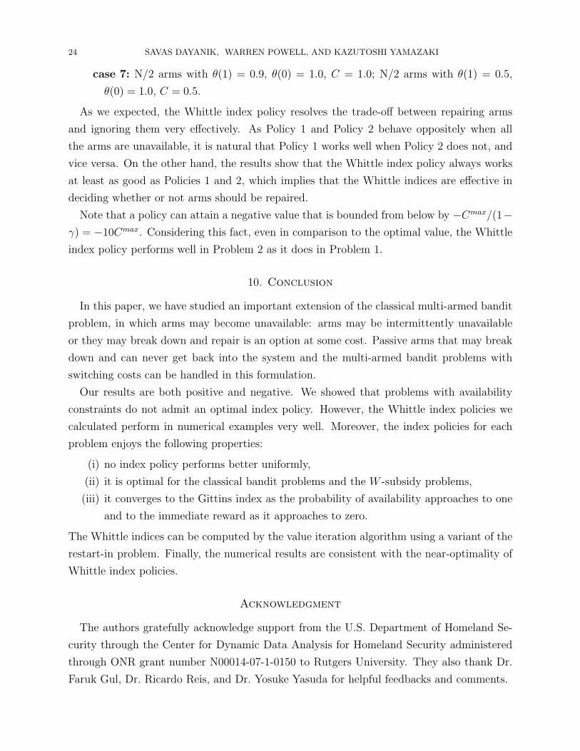
case 7: N/2 arms with θ(1) = 0.9, θ(0) = 1.0, C = 1.0; N/2 arms with θ(1) = 0.5,
θ(0) = 1.0, C = 0.5.
As we expected, the Whittle index policy resolves the trade-off between repairing arms
and ignoring them very effectively. As Policy 1 and Policy 2 behave oppositely when all
the arms are unavailable, it is natural that Policy 1 works well when Policy 2 does not, and
vice versa. On the other hand, the results show that the Whittle index policy always works
at least as good as Policies 1 and 2, which implies that the Whittle indices are effective in
deciding whether or not arms should be repaired.
Note that a policy can attain a negative value that is bounded from below by −Cmax/(1−γ) = −10Cmax. Considering this fact, even in comparison to the optimal value, the Whittle
index policy performs well in Problem 2 as it does in Problem 1.
10. Conclusion
In this paper, we have studied an important extension of the classical multi-armed bandit
problem, in which arms may become unavailable: arms may be intermittently unavailable
or they may break down and repair is an option at some cost. Passive arms that may break
down and can never get back into the system and the multi-armed bandit problems with
switching costs can be handled in this formulation.
Our results are both positive and negative. We showed that problems with availability
constraints do not admit an optimal index policy. However, the Whittle index policies we
calculated perform in numerical examples very well. Moreover, the index policies for each
problem enjoys the following properties:
(i) no index policy performs better uniformly,
(ii) it is optimal for the classical bandit problems and the W -subsidy problems,
(iii) it converges to the Gittins index as the probability of availability approaches to one
and to the immediate reward as it approaches to zero.
The Whittle indices can be computed by the value iteration algorithm using a variant of the
restart-in problem. Finally, the numerical results are consistent with the near-optimality of
Whittle index policies.
Acknowledgment
The authors gratefully acknowledge support from the U.S. Department of Homeland Se-
curity through the Center for Dynamic Data Analysis for Homeland Security administered
through ONR grant number N00014-07-1-0150 to Rutgers University. They also thank Dr.
Faruk Gul, Dr. Ricardo Reis, and Dr. Yosuke Yasuda for helpful feedbacks and comments.
BANDIT PROBLEM WITH AVAILABILITY CONSTRAINTS 25
Appendix A. Proofs
A.1. Proof of Proposition 4.1. Consider the W -subsidy problem with fixed W ∈ R. The
main argument in this proof is that if the process (X, Y ) enters a state (x, 1) for some x ∈ X(and the arm is available) and if it is optimal to take the passive action, then it must be
optimal to take the passive action at every stage after that.
Consider (X, Y ) with initial state (X(0), Y (0)) = (x, 1). Let us suppose (x, 1) ∈ Π(W ),
meaning that it is optimal to take the passive action if the arm is in state (x, 1). Note that
X does not change under the passive action, and that when it becomes unavailable (when it
enters (x, 0)) it is also optimal to make it passive by Condition 4.1. Consequently, when the
arm becomes available, the new state is again (x, 1). As we are assuming that (x, 1) ∈ Π(W ),
the passive action is optimal again. Consequently, once the process (X, Y ) enters the state
(x, 1) ∈ Π(W ), the arm must stay passive forever.
Therefore, the W-subsidy problem is reduced to an optimal stopping problem; finding
the best time when the arm is available to switch to the passive action. We restrict our
attention to (Ft)t≥0-stopping times τ such that Y (τ) = 1 almost surely, and consider the
following strategy: until time τ − 1, activate the arm if it is available and choose the passive
action otherwise; at and after time τ always choose the passive action. The expected total
discounted reward of this strategy is
E1,0x,1
[τ−1∑t=0
γt(RY (t)(X(t), Y (t)) +W1{Y (t)=0}
)+
∞∑t=τ
γtW + γτρ(X(τ), Y (τ))
].
On the other hand, stopping immediately in state (x, 1) gives∑∞
t=0 γtW + ρ(x, 1) = W/(1−
γ) + ρ(x, 1). Therefore, (x, 1) ∈ Π(W ) if and only if, for every τ ∈ S we have
(26)W
1− γ+ ρ(x, 1) ≥ E1,0
x,1
[τ−1∑t=0
γt(RY (t)(X(t), Y (t)) +W1{Y (t)=0}
)+ γτρ(X(τ), Y (τ)) +
∞∑t=τ
γtW
].
Moreover, the expectation on the right-hand side equals
E1,0x,1
[τ−1∑t=0
γtRY (t)(X(t), Y (t)) + γτρ(X(τ), Y (τ))
]+WE1,0
x,1
[τ−1∑t=1
γt1{Y (t)=0} +γτ
1− γ
].(27)
Substituting (27) into (26) and some algebra give
W ≥ (1− γ)E1,0
x,1
[∑τ−1t=0 γ
tRY (t)(X(t), Y (t)) + γτρ(X(τ), Y (τ))]− ρ(x, 1)
1− E1,0x,1
[(1− γ)
∑τ−1t=1 γ
t1{Y (t)=0} + γτ] ,
for every τ ∈ S. Thus, (x, 1) ∈ Π(W ) if and only if (7) holds.
26 SAVAS DAYANIK, WARREN POWELL, AND KAZUTOSHI YAMAZAKI
A.2. Proof of Proposition 4.2. Firstly, the Whittle index when the arm is not available
follows from its definition and Condition 4.1. Now consider the case when the arm is available.
By Proposition 4.1, (x, 1) ∈ Π(W ) if and only if (7) is satisfied. Therefore,
W1 > W2 =⇒ {(x, 1); (x, 1) ∈ Π(W1)} ⊇ {(x, 1); (x, 1) ∈ Π(W2)},
and by Condition 4.1 W1 > W2 =⇒ Π(W1) ⊇ Π(W2); therefore, the arm is indexable, and
W (x, 1) ≡ inf{W : (x, 1) ∈ Π(W )} coincides with the Whittle index.
A.3. Proof of Corollary 4.1. If Y (0) = 1, then by Condition 4.2 P1,0-a.s Y (t) = 1, t ≥ 0.
Thus, S can be replaced by S. Substituting 1{Y (t)=0} = 0 into (8) completes the proof.
A.4. Proof of Corollary 4.3. We obtain (11) after substituting into (10) the expression
(28) E1,0x,1
[τ−1∑t=1
γt1{Y (t)=0}
]= E1,0
x,1
[∞∑
t=1
γt1{Y (t)=0}1{t<τ}
]=
∞∑t=1
E1,0x,1
[γt1{Y (t)=0}1{t<τ}
]=
∞∑t=1
γtE1,0x,1
[1{Y (t)=0}
]E1,0
x,1
[1{t<τ}
]=
∞∑t=1
γt(1− θ)E1,0x,1
[1{t<τ}
]= E1,0
x,1
[τ−1∑t=1
(1− θ)γt
].
A.5. Proof of Corollary 4.4. If Y (0) = 1, then Y (t) = 1, P1,0-almost surely, for every
t ≥ 0 by (12). Therefore, S is the same as S, and after plugging θ ≡ 1 in (11), we obtain
W (x, 1) = (1− γ) supτ∈S
E1,0x,1
[∑τ−1t=0 γ
tR1(X(t), Y (t))]
1− E1,0x,1 [γτ ]
= supτ∈S
E1,0x,1
[∑τ−1t=0 γ
tR1(X(t), Y (t))]
E1,0x,1
[∑τ−1t=0 γ
t] .
A.6. Proof of Proposition 4.3. Only in this proof, in order to emphasize the dependence
of W and P1,0 on θ ∈ [0, 1], we replace them with Wθ and Pθ, respectively. Therefore,
Wθ(x, y) =
(1− γ) sup
τ∈S
Γ(θ, τ, x) ,Eθ
x,1
[∑τ−1t=0 γ
tR1(X(t), Y (t))1{Y (t)=1}]
1− γ(1− θ)− θEθx,1 [γτ ]
, if y = 1,
−∞, otherwise.
The Gittins index corresponds to M(x) = W1(x, 1) ≡ (1 − γ) supτ∈S Γ(1, τ, x). Let R be a
finite constant such that |R(x, 1)| < R for every x ∈ X .
We first prove the convergence to the immediate reward as θ ↘ 0. As immediate stopping
attains R1(x, 1), we have Wθ(x, 1) ≥ R(x, 1). Let
Wθ(x, 1) , supτ∈S
Eθx,1
[τ−1∑t=0
γtR1(X(t), Y (t))1{Y (t)=1}
].
Because (1 − γ) ≤ 1− γ(1− θ)− θE1,0x,1 [γτ ] for every τ ∈ S, we have Wθ(x, 1) ≥ Wθ(x, 1).
Therefore, it is sufficient to show that W (x, 1) − R1(x, 1) → 0 as θ → 0. Let K be the
BANDIT PROBLEM WITH AVAILABILITY CONSTRAINTS 27
next time the arm is available. Then Pθ {K = k} = (1 − θ)k−1θ, k ≥ 1 and Eθ[γK]
=
θγ/(1− γ(1− θ)) ≤ θγ/(1− γ); therefore,
W (x, 1) ≤ R1(x, 1) + E1,0x,1
[γK
∞∑t=0
γtR
]< R1(x, 1) + θ
Rγ
(1− γ)2
and R1(x, 1) ≤ Wθ(x, 1) ≤ Wθ(x, 1) < R1(x, 1) + θRγ/(1 − γ)2 holds for every x ∈ X , and
Wθ(x, 1) converges to the immediate reward R1(x, 1) as θ ↘ 0 uniformly over x ∈ X . To
show the convergence to the Gittins index as θ ↗ 1, we will need the following lemma.
Lemma A.1. There is a finite constant B such that supτ∈S, x∈X |Γ(1, τ, x)− Γ(θ, τ, x)| <B(1− θ).
Proof. For θ ∈ (0, 1), τ ∈ S, and x ∈ X , the difference |Γ(1, τ, x)− Γ(θ, τ, x)| equals∣∣∣∣∣E1x,1
[∑τ−1t=0 γ
tR1(X(t), Y (t))]
1− E1x,1 [γτ ]
−Eθ
x,1
[∑τ−1t=0 γ
tR1(X(t), Y (t))1{Y (t)=1}]
1− γ(1− θ)− θEθx,1 [γτ ]
∣∣∣∣∣≤
∣∣∣∣∣E1x,1
[∑τ−1t=0 γ
tR1(X(t), Y (t))]
1− E1x,1 [γτ ]
−Eθ
x,1
[∑τ−1t=0 γ
tR1(X(t), Y (t))1{Y (t)=1}]
1− E1x,1 [γτ ]
∣∣∣∣∣+
∣∣∣∣∣Eθx,1
[∑τ−1t=0 γ
tR1(X(t), Y (t))1{Y (t)=1}]
1− E1x,1 [γτ ]
−Eθ
x,1
[∑τ−1t=0 γ
tR1(X(t), Y (t))1{Y (t)=1}]
1− γ(1− θ)− θEθx,1 [γτ ]
∣∣∣∣∣=
∣∣E1x,1
[∑τ−1t=0 γ
tR1(X(t), Y (t))]− Eθ
x,1
[∑τ−1t=0 γ
tR1(X(t), Y (t))1{Y (t)=1}]∣∣
1− E1x,1 [γτ ]
+ Eθx,1
[τ−1∑t=0
γtR1(X(t), Y (t))1{Y (t)=1}
] ∣∣∣∣ 1
1− E1x,1 [γτ ]
− 1
1− γ(1− θ)− θEθx,1 [γτ ]
∣∣∣∣≤∣∣E1
x,1
[∑τ−1t=0 γ
tR1(X(t), Y (t))]− Eθ
x,1
[∑τ−1t=0 γ
tR1(X(t), Y (t))1{Y (t)=1}]∣∣
1− γ
+R
1− γ
∣∣∣∣ 1
1− E1x,1 [γτ ]
− 1
1− γ(1− θ)− θEθx,1 [γτ ]
∣∣∣∣ .Now it is sufficient to prove that there exist some finite numbers B1 and B2 such that
(i)∣∣E1
x,1
[∑τ−1t=0 γ
tR1(X(t), Y (t))]− Eθ
x,1
[∑τ−1t=0 γ
tR1(X(t), Y (t))1{Y (t)=1}]∣∣ ≤ B1(1− θ),
(ii)∣∣∣ 11−E1
x,1[γτ ]− 1
1−γ(1−θ)−θEθx,1[γτ ]
∣∣∣ ≤ B2(1− θ).
To this end, let L be the first time the arm is unavailable. Note that for every l ≥ 1,
the joint conditional Pθ-distribution of {(X(t), Y (t)); 0 ≤ t ≤ l − 1} given L = l is the
same as the joint unconditional P1-distribution of {(X(t), Y (t)); 0 ≤ t ≤ l − 1}, and we have
Pθ {L = l} = θl−1(1− θ), l ≥ 1 and Eθx,1
[γL]
= γ(1− θ)/(1− γθ) < (1− θ)γ/(1− γ). The
28 SAVAS DAYANIK, WARREN POWELL, AND KAZUTOSHI YAMAZAKI
inequality in (i) holds with B1 = (1− θ)2γR/(1− γ)2 because
∣∣∣∣∣E1x,1
[τ−1∑t=0
γtR1(X(t), Y (t))
]− Eθ
x,1
[τ−1∑t=0
γtR1(X(t), Y (t))1{Y (t)=1}
]∣∣∣∣∣≤
∞∑l=1
Pθx,1 {L = l}
∣∣∣∣∣E1x,1
[τ−1∑t=0
γtR1(X(t), Y (t))
]− Eθ
x,1
[τ−1∑t=0
γtR1(X(t), Y (t))1{Y (t)=1}
∣∣∣∣∣L = l
]∣∣∣∣∣ ,where for every l ≥ 1, the absolute difference can be rewritten as
∣∣∣∣∣E1x,1
[τ−1∑t=0
γtR1(X(t), Y (t))1{τ≤l−1}
]− Eθ
x,1
[τ−1∑t=0
γtR1(X(t), Y (t))1{Y (t)=1}1{τ≤l−1}
∣∣∣∣∣L = l
]
+ E1x,1
[τ−1∑t=0
γtR1(X(t), Y (t))1{τ>l−1}
]− Eθ
x,1
[τ−1∑t=0
γtR1(X(t), Y (t))1{Y (t)=1}1{τ>l−1}
∣∣∣∣∣L = l
]∣∣∣∣∣=
∣∣∣∣∣E1x,1
[τ−1∑t=0
γtR1(X(t), Y (t))1{τ>l−1}
]− Eθ
x,1
[τ−1∑t=0
γtR1(X(t), Y (t))1{Y (t)=1}1{τ>l−1}
∣∣∣∣∣L = l
]∣∣∣∣∣≤
∣∣∣∣∣E1x,1
[l−1∑t=0
γtR1(X(t), Y (t))1{τ>l−1}
]− Eθ
x,1
[l−1∑t=0
γtR1(X(t), Y (t))1{Y (t)=1}1{τ>l−1}
∣∣∣∣∣L = l
]∣∣∣∣∣+
∣∣∣∣∣E1x,1
[τ−1∑t=l
γtR1(X(t), Y (t))1{τ>l−1}
]− Eθ
x,1
[τ−1∑t=l
γtR1(X(t), Y (t))1{Y (t)=1}1{τ>l−1}
∣∣∣∣∣L = l
]∣∣∣∣∣=
∣∣∣∣∣E1x,1
[τ−1∑t=l
γtR1(X(t), Y (t))1{τ>l−1}
]− Eθ
x,1
[τ−1∑t=l
γtR1(X(t), Y (t))1{Y (t)=1}1{τ>l−1}
∣∣∣∣∣L = l
]∣∣∣∣∣which is less than
∑∞t=l γ
t2R; therefore, the left-hand side of (i) is less than or equal to
∞∑l=1
Pθx,1 {L = l}
∞∑t=l
γt2R =2R
1− γEθ
x,1
[γL]
= (1− θ)2γR
(1− γ)2.
The inequality in (ii) holds with B2 = γ(1− θ)/(1− γ)2 because
∣∣∣∣ 1
1− E1x,1 [γτ ]
− 1
1− γ(1− θ)− θEθx,1 [γτ ]
∣∣∣∣ =
∣∣∣∣∣ −γ(1− θ)− θEθx,1 [γτ ] + E1
x,1 [γτ ](1− E1
x,1 [γτ ]) (
1− γ(1− θ)− θEθx,1 [γτ ]
)∣∣∣∣∣≤γ(1− θ) + θ
∣∣Eθx,1 [γτ ]− E1
x,1 [γτ ]∣∣+ (1− θ)E1
x,1 [γτ ](1− E1
x,1 [γτ ]) (
1− γ(1− θ)− θEθx,1 [γτ ]
) ≤(γ + 1)(1− θ) +
∣∣Eθx,1 [γτ ]− E1
x,1 [γτ ]∣∣
(1− γ)2,
BANDIT PROBLEM WITH AVAILABILITY CONSTRAINTS 29
and∣∣E1
x,1 [γτ ]− Eθx,1 [γτ ]
∣∣ ≤∑∞n=1 Pθ
x,1 {L = l}∣∣E1
x,1 [γτ ]− Eθx,1 [γτ |L = l]
∣∣ equals
∞∑n=1
Pθx,1 {L = l}
∣∣E1x,1
[γτ1{τ≤l−1}
]− Eθ
x,1
[γτ1{τ≤l−1}|L = l
]+E1
x,1
[γτ1{τ>l−1}
]− Eθ
x,1
[γτ1{τ>l−1}|L = l
]∣∣=
∞∑n=1
Pθx,1 {L = l}
∣∣E1x,1
[γτ1{τ>l−1}
]− Eθ
x,1
[γτ1{τ>l−1}|L = l
]∣∣=
∞∑n=1
Pθx,1 {L = l}
∞∑t=l
γt∣∣P1
x,1 {τ = t} − Pθx,1 {τ = t|L = l}
∣∣≤
∞∑n=1
Pθx,1 {L = l}
∞∑t=l
γt =1
1− γEθ
x,1
[γL]< (1− θ)
γ
(1− γ)2.
Therefore, the conclusion of Lemma A.1 follows if B , B1/(1− γ) +B2R/(1− γ). �
Fix x ∈ X . Let τ 1(x) and τ θ(x) attain M(x) = supτ∈S Γ(1, τ, x) and Wθ(x, 1) =
supτ∈S Γ(θ, τ, x), respectively. Then Lemma A.1 implies that
Γ(1, τ 1(x), x) ≥ Γ(1, τ θ(x), x) ≥ Γ(θ, τ θ(x), x)−B(1− θ)
≥ Γ(θ, τ 1(x), x)−B(1− θ) ≥ Γ(1, τ 1(x), x)− 2B(1− θ),
which completes the proof of Proposition 4.3 because
supx∈X
|M(x)−Wθ(x, 1)| = supx∈X
∣∣Γ(1, τ 1(x), x)− Γ(θ, τ θ(x), x)∣∣ ≤ 2B(1 − θ)
θ↑1−−→ 0.
A.7. Proof of Proposition 4.4. The W -subsidy problem is a special case of Problem 1.
To see this, consider the situation where there are only two arms; arm 1 follows a generic
stochastic process (X(t), Y (t)) as defined in Section 2, and arm 2 is always available and
gives a constant reward a. Let (x1, 1) and (x2, 0) denote the current state of arm 1 and
arm 2, respectively. Therefore, by Proposition 4.1 it is optimal to rest the arm if and only
if a ≥ W (x1, 1). That is, the index of arm 1 must be a strict monotone transformation of
W (x1, 1) and that of arm 2 must be a monotone transformation of a. The process (X(t), Y (t))
of arm 1 is general, and any arm in the problem class has to satisfy the above mentioned
property. Moreover,
W (x2, 1) = (1− γ) supτ∈S
E1,0x2,1
[∑τ−1t=0 γ
tR1(X(t), Y (t))1{Y (t)=1}]
1− E1,0x2,1
[∑τ−1t=1 (1− γ)γt1{Y (t)=0} + γτ
] = supτ∈S
E1,0x2,1
[∑τ−1t=0 γ
ta]
E1,0x2,1
[∑τ−1t=0 γ
t] = a.
Since any optimal index W (·, ·) must also be optimal on every W -subsidy problem, it is
immediate that any such index must be a strict monotone transformation of W (·, ·).
30 SAVAS DAYANIK, WARREN POWELL, AND KAZUTOSHI YAMAZAKI
A.8. Proof of Proposition 4.5. We give a counterexample in which an arm is available
now, but its future availability is highly unlikely: consider the case with two arms where
arm 1 is always available, and arm 2 is available with probability ε ∈ (0, 1). Suppose that
passive arms do not give rewards and M = 1.
The reward from arm 1 changes deterministically under the active action
1 → 100 → 10 → 10 → . . .→ 10 → . . . .
Let the corresponding states be x11, x12, x13, . . . . On the other hand, arm 2 does not change
its state and it gives a constant reward 40 whenever it is available. Denote its state by
x2. Suppose both arm 1 and arm 2 are currently available, and their states are x11 and x2,
respectively. Let ε = 0.01 and γ = 0.7. After obvious choices of stopping times τ in (11),
the index for arm 1 satisfies the bounds
W1(x11, 1) ≥ 1 + γ100
1 + γ= 41.76, W1(x12, 1) ≥ 100
1= 100, W1(x1n, 1) = 10, n ≥ 3,(29)
and the indices for arm 2 must satisfy W2(x2, 1) = 40 and W2(x2, 0) = −∞.
For contradiction, assume that the index policy defined by (11) is optimal. Then arm
1 must be pulled, if X1 = x11; arm 1 must be pulled, if X1 = x12; arm 2 must be pulled
whenever it is available and arm 1 must be pulled otherwise, if X1 = x13, . . .. That is, the
optimal policy is to pull arm 1 twice (at X1 = x11 and x12) and then pull arm 2 whenever it
is available and arm 1 otherwise. Therefore, the value function must satisfy
V ((x11, 1), (x2, 1)) = 1 + γ100 + γ2 {10(1− ε) + 40ε}+ γ3 {10(1− ε) + 40ε}+ . . . .
= 1 + γ100 + γ2
∞∑k=0
{γk(10 + 30ε)
}≈ 87.8233,
and V ((x11, 1), (x2, 0)) = V ((x11, 1), (x2, 1)); however, pulling arm 2 at ((x11, 1), (x2, 1)) gives
40 + γ {εV ((x11, 1), (x2, 1)) + (1− ε)V ((x11, 1), (x2, 0))} ≈ 101.4763 > V ((x11, 1), (x2, 1)).
This contradicts with the optimality of V . Therefore, the index policy given by (11) cannot
be optimal, and by Proposition 4.4 no optimal index policy exists for Problem 1 in general.
A.9. Proof of Proposition 5.1. We prove the indexability and obtain the Whittle index
of the arm under Condition 5.1. We consider the cases W < −C(x) and W ≥ −C(x)
separately after the following two lemmas.
Lemma A.2. For every x ∈ X and W ∈ R, if (x, 0) ∈ Π(W ), then V ((x, 0),W ) = W/(1−γ), which is obtained by taking the passive action all the time.
BANDIT PROBLEM WITH AVAILABILITY CONSTRAINTS 31
Proof. Both X and Y do not change under the passive action. If (x, 0) ∈ Π(W ), then the
passive action remains optimal forever. Consequently, the expected total discounted reward
starting in (x, 0) becomes V ((x, 0),W ) =∑∞
t=0 γtW = W/(1− γ). �
Lemma A.3. For every x ∈ X and W ∈ R, if (x, 1) ∈ Π(W ), then the stochastic process
(X, Y ) starting in (x, 1) visits only (x, 1) and/or (x, 0) under the optimal policy, and
V ((x, 1),W ) = max
{E0,1
x,1
[∞∑
t=0
γt{W1{Y (t)=1} − C(x)1{Y (t)=0}
}],W
1− γ
},(30)
where P0,1 is the probability law induced by the policy that activates the arm as long as it is
unavailable and leaves it in rest otherwise.
Proof. First, note that X does not change under the passive action and when the arm is not
available. Therefore, the next time the arm is available, X = x. As we are assuming that
(x, 1) ∈ Π(W ), the passive action must be taken whenever the arm is available. Therefore,
only (x, 0) and (x, 1) will be visited by the process.
Now the optimal policy must be one of the following two: the policy under which the arm
is passive when it is in state (x, 1) or in (x, 0), and the policy under which the arm is passive
when it is in (x, 1), but is active when it is in (x, 0). The value under the former policy is
W/(1− γ) by Lemma A.2, and the value under the latter is the expectation in (30). �
Lemma A.4. If W < −C(x), and Condition 5.2 holds, then (x, y) /∈ Π(W ) for every
y ∈ {0, 1}; therefore, Π(W ) = ∅.
Proof. Suppose that (x, 0) ∈ Π(W ) for some x ∈ X . By Lemma A.2,
V ((x, 0),W ) = W/(1− γ).(31)
However, a lower bound on V ((x, 0),W ) can be obtained by considering the policy under
which the arm is active at (x, 0) and passive otherwise. Because W < −C(x), this policy
gives V ((x, 0),W ) > W/(1− γ), which contradicts with (31) and implies that
(x, 0) /∈ Π(W ), x ∈ X .(32)
Suppose now (x, 1) ∈ Π(W ) for some x ∈ X . Then, by Lemma A.3 and (32), we obtain
V ((x, 1),W ) = E0,1x,1
[∞∑
t=0
γt{W1{Y (t)=1} − C(x)1{Y (t)=0}
}]≤ −C(x)
1− γ.
However, this contradicts with the lower bound obtained by applying the policy under which
the arm is always active; namely,
V ((x, 1),W ) = E1,1x,1
[∞∑
t=0
γt{R1(X(t), Y (t))1{Y (t)=1} − C(X(t))1{Y (t)=0}
}]> −C(x)
1− γ,
32 SAVAS DAYANIK, WARREN POWELL, AND KAZUTOSHI YAMAZAKI
where the last inequality holds under Condition 5.2. Therefore, (x, 1) /∈ Π(W ), x ∈ X . �
Lemma A.5. If W ≥ −C(x), then (x, y) ∈ Π(W ) if and only if, for every τ ∈ S,
W ≥ (1− γ)E1,1
x,y
[∑τ−1t=0 γ
tR1(X(t), Y (t))]
1− E1,1x,y [γτ ]
.
Proof. The main argument in the proof is that in the W -subsidy problem, once the passive
action is optimal, it remains optimal to take the passive action thereafter. This follows for
y = 0 immediately from Lemma A.2.
Suppose now (x, 1) ∈ Π(W ) for some x ∈ X . By Lemma A.3, starting at (x, 1) under the
optimal policy, only (x, 0) and (x, 1) will be visited by the process (X,Y ), and (30) holds.
Moreover, W ≥ −C(x) implies
E0,1x,1
[∞∑
t=0
γt{W1{Y (t)=1} − C(x)1{Y (t)=0}
}]≤ W
1− γ;
thus, V ((x, 1),W ) = W/(1− γ), and the optimal policy always chooses the passive action.
Using the argument above, the W -subsidy problem is reduced to an optimal stopping
problem as in the proof of Proposition 4.2. The optimal strategy must choose the active
action until some stopping time τ and choose the passive action at and after time τ . The
main difference with Problem 1 is that it may be optimal to stop even when Y = 0. If
we switch from the active action to the passive action at some stopping time τ , then the
expected total discounted reward will be
E1,1x,y
[τ−1∑t=0
R1(X(t), Y (t)) +∞∑
t=τ
γtW
].
As in the proof of Proposition 4.2, (x, y) ∈ Π(W ) if and only if immediate stopping achieves
greater value than the displayed expectation for any positive stopping time τ ∈ S. Since
immediate stopping yields W/(1− γ), we have (x, y) ∈ Π(W ) if and only if
W
1− γ≥ E1,1
x,y
[τ−1∑t=0
R1(X(t), Y (t)) +∞∑
t=τ
γtW
]for every τ ∈ S. �
Proposition 5.1 follows immediately from Lemmas A.4 and A.5.
A.10. Proof of Proposition 5.2. The monotonicity of W 7→ Π(W ) is clear by Proposition
5.1; therefore, the arm is indexable. By Proposition 5.1 and by definition of the Whittle
index (4), the Whittle index at (x, y) is given by (16).
BANDIT PROBLEM WITH AVAILABILITY CONSTRAINTS 33
A.11. Proof of Proposition 5.4. Consider a variant of the situation in the proof for
Proposition 4.5 (see Proof of Proposition 4.5 in A.8) with the same value of ε and γ. Arm
1 is defined the same as in the proof of Proposition 4.5, and arm 2 again gives a constant
reward 40 whenever it is available. Arm 2 breaks down with probability (1 − ε), and it is
repaired with probability 1 the next time when it is repaired. The repair costs C = 100.
The index for arm 1 still satisfies the inequalities in (29) while the index for arm 2 satisfies
W2(x2, 1) ≤ 40, and
W2(x2, 0) = supτ∈S
E1,1x2,0
[∑τ−1t=0 γ
tR(X(t), Y (t))]
E1,1x2,0
[∑τ−1t=0 γ
t] ≤ sup
τ∈SE1,1
x2,0
[τ−1∑t=0
γtR(X(t), Y (t))
]
≤ −C + γ40 + γ240 + . . . = −C +40γ
1− γ≤ 10.
Therefore, the index policy pulls arm 1 twice (at X1 = x11 and x12) and then arm 2 whenever
it is available and arm 1 otherwise. Therefore, the value function satisfies
V ((x11, 1), (x2, 1)) = 1 + γ100 + γ2{10(1− ε2) + 40ε2
}+ γ3
{10(1− ε3) + 40ε3
}+ . . . .
= 1 + γ100 + γ2
∞∑k=0
{γk(10 + 30εk
)}≈ 102.1370,
and V ((x11, 1), (x2, 0)) = V ((x11, 1), (x2, 1)); however, pulling arm 2 at ((x11, 1), (x2, 1)) gives
40 + γ {εV ((x11, 1), (x2, 1)) + (1− ε)V ((x11, 1), (x2, 0))} = 111.4959 > V ((x11, 1), (x2, 1)),
which contradicts with the optimality of V . Therefore, the index policy defined by (16)
cannot be optimal, and by Proposition 5.3 there is no optimal index policy for Problem 2.
A.12. Proof of Proposition 6.1. Since νx,1 = (1 − γ)R1(x, 1) + γ∑
x′∈X pxx′ [θ1(x, 1)νx′,1
+(1− θ1(x, 1))νx′,0], we have
νx,1 = max
{(1− γ)R1(x, 1) + γ
∑x′∈S
pxx′[θ1(x, 1)νx′,1 + (1− θ1(x, 1))νx′,0
], νx,1
}, x ∈ X .
Together with (20), it is easy to see that
νx,1 = supτ∈S
E1,0x,1
[τ−1∑t=0
γt((1− γ)R1(X(t), Y (t))1{Y (t)=1} + (1− γ)νx,11{Y (t)=0}
)+ γτνx,1
],
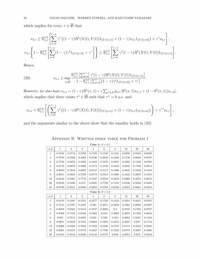
34 SAVAS DAYANIK, WARREN POWELL, AND KAZUTOSHI YAMAZAKI
which implies for every τ ∈ S that
νx,1 ≥ E1,0x,1
[τ−1∑t=0
γt((1− γ)R1(X(t), Y (t))1{Y (t)=1} + (1− γ)νx,11{Y (t)=0}
)+ γτνx,1
],
νx,1
{1− E1,0
x,1
[τ−1∑t=0
(1− γ)γt1{Y (t)=0} + γτ
]}≥ E1,0
x,1
[τ−1∑t=0
γt(1− γ)R1(X(t), Y (t))1{Y (t)=1}
].
Hence,
νx,1 ≥ supτ∈S
E1,0x,1
[∑τ−1t=0 γ
t(1− γ)R1(X(t), Y (t))1{Y (t)=1}]
1− E1,0x,1
[∑τ−1t=0 (1− γ)γt1{Y (t)=0} + γτ
] .(33)
However, we also have νx,1 = (1−γ)R1(x, 1)+γ∑
x′∈X pxx′ [θ1(x, 1)νx′,1 + (1− θ1(x, 1))νx′,0],
which implies that there exists τ ∗ ∈ S such that τ ∗ > 0 a.s. and
νx,1 = E1,0x,1
[(τ∗−1∑t=0
γt((1− γ)R1(X(t), Y (t))1{Y (t)=1} + (1− γ)νx,11{Y (t)=0}
))+ γτ∗
νx,1
],
and the arguments similar to the above show that the equality holds in (33).
Appendix B. Whittle index table for Problem 1
Case 1: θ = 0.1
a\b 1 2 3 4 6 8 10 20 40
1 0.5534 0.3713 0.2766 0.2193 0.1540 0.1181 0.0956 0.0484 0.0238
2 0.7019 0.5320 0.4263 0.3546 0.2643 0.2100 0.1740 0.0929 0.0475
3 0.7740 0.6255 0.5226 0.4483 0.3479 0.2837 0.2392 0.1332 0.0700
4 0.8172 0.6870 0.5909 0.5174 0.4139 0.3443 0.2945 0.1700 0.0914
6 0.8670 0.7634 0.6807 0.6137 0.5117 0.4386 0.3835 0.2346 0.1313
8 0.8951 0.8093 0.7378 0.6773 0.5814 0.5088 0.4522 0.2897 0.1678
10 0.9132 0.8401 0.7772 0.7227 0.6334 0.5633 0.5069 0.3373 0.2013
20 0.9529 0.9108 0.872 0.8035 0.7729 0.7182 0.6706 0.5030 0.3348
40 0.9749 0.9521 0.9303 0.9094 0.8703 0.8520 0.8012 0.6681 0.5010
Case 2: θ = 0.3
a\b 1 2 3 4 6 8 10 20 40
1 0.6135 0.4191 0.3131 0.2477 0.1726 0.1313 0.1054 0.0521 0.0255
2 0.7414 0.5707 0.4594 0.383 0.2851 0.2259 0.1865 0.0983 0.0497
3 0.8023 0.6564 0.5513 0.4737 0.3682 0.3 0.2525 0.1395 0.0727
4 0.8388 0.7123 0.6156 0.5403 0.433 0.3602 0.3078 0.1768 0.0944
6 0.881 0.7814 0.6995 0.632 0.528 0.453 0.3962 0.2481 0.1348
8 0.9051 0.8229 0.7524 0.6922 0.5955 0.5215 0.4637 0.297 0.1716
10 0.9208 0.8508 0.7892 0.7352 0.6456 0.5747 0.5174 0.3444 0.2053
20 0.9561 0.9155 0.8778 0.8427 0.7798 0.7252 0.6775 0.5087 0.3388
40 0.9763 0.9542 0.9328 0.9123 0.8737 0.838 0.8051 0.672 0.5042
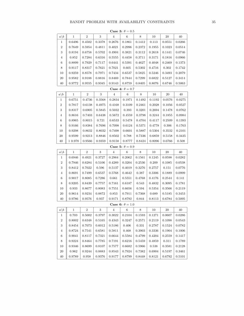
BANDIT PROBLEM WITH AVAILABILITY CONSTRAINTS 35
Case 3: θ = 0.5
a\b 1 2 3 4 6 8 10 20 40
1 0.6496 0.4502 0.3378 0.2676 0.1861 0.1412 0.113 0.0551 0.0266
2 0.7649 0.5954 0.4811 0.4021 0.2996 0.2372 0.1955 0.1023 0.0514
3 0.8194 0.6758 0.5702 0.4904 0.3821 0.3112 0.2618 0.1441 0.0746
4 0.852 0.7284 0.6316 0.5555 0.4458 0.3711 0.3171 0.1816 0.0966
6 0.8899 0.7929 0.7117 0.6441 0.5391 0.4627 0.4048 0.2469 0.1373
8 0.9117 0.8317 0.7621 0.7021 0.605 0.5302 0.4716 0.302 0.1742
10 0.9259 0.8578 0.7971 0.7434 0.6537 0.5825 0.5246 0.3493 0.2079
20 0.9582 0.9188 0.8816 0.8469 0.7844 0.7299 0.6822 0.5127 0.3414
40 0.9772 0.9555 0.9345 0.9143 0.8759 0.8405 0.8076 0.6746 0.5063
Case 4: θ = 0.7
a\b 1 2 3 4 6 8 10 20 40
1 0.6751 0.4736 0.3568 0.2834 0.1971 0.1492 0.1192 0.0576 0.0275
2 0.7817 0.6138 0.4975 0.4168 0.3109 0.2461 0.2028 0.1056 0.0527
3 0.8317 0.6905 0.5845 0.5032 0.393 0.3201 0.2694 0.1478 0.0762
4 0.8616 0.7403 0.6438 0.5672 0.4559 0.3798 0.3244 0.1855 0.0984
6 0.8965 0.8015 0.721 0.6533 0.5478 0.4704 0.4117 0.2509 0.1393
8 0.9166 0.8384 0.7696 0.7098 0.6124 0.5371 0.4778 0.306 0.1763
10 0.9298 0.8632 0.8032 0.7498 0.6601 0.5887 0.5304 0.3532 0.2101
20 0.9599 0.9213 0.8846 0.8502 0.788 0.7336 0.6859 0.5158 0.3435
40 1 0.978 0.9566 0.9359 0.9158 0.8777 0.8424 0.8096 0.6766 0.508
Case 5: θ = 0.9
a\b 1 2 3 4 6 8 10 20 40
1 0.6946 0.4921 0.3727 0.2964 0.2062 0.1561 0.1245 0.0598 0.0282
2 0.7946 0.6284 0.5106 0.4289 0.3204 0.2536 0.209 0.1085 0.0538
3 0.8412 0.7022 0.596 0.5137 0.4019 0.3276 0.2757 0.151 0.0776
4 0.8691 0.7499 0.6537 0.5768 0.4642 0.387 0.3306 0.1889 0.0999
6 0.9017 0.8085 0.7286 0.661 0.5551 0.4768 0.4176 0.2544 0.141
8 0.9205 0.8439 0.7757 0.7161 0.6187 0.543 0.4832 0.3095 0.1781
10 0.933 0.8677 0.8083 0.7551 0.6656 0.594 0.5354 0.3566 0.2119
20 0.9614 0.9234 0.8872 0.853 0.7911 0.7368 0.689 0.5185 0.3453
40 0.9786 0.9576 0.937 0.9171 0.8792 0.844 0.8113 0.6784 0.5095
Case 6: θ = 1.0
a\b 1 2 3 4 6 8 10 20 40
1 0.703 0.5002 0.3797 0.3022 0.2104 0.1593 0.1271 0.0607 0.0286
2 0.8002 0.6348 0.5165 0.4343 0.3247 0.2571 0.2119 0.1098 0.0543
3 0.8454 0.7073 0.6012 0.5186 0.406 0.331 0.2787 0.1524 0.0782
4 0.8724 0.7541 0.6581 0.5811 0.468 0.3903 0.3336 0.1904 0.1006
6 0.9041 0.8117 0.7321 0.6644 0.5584 0.4799 0.4204 0.2559 0.1417
8 0.9224 0.8464 0.7785 0.7191 0.6216 0.5459 0.4859 0.311 0.1789
10 0.9346 0.8699 0.8107 0.7577 0.6682 0.5966 0.538 0.3581 0.2128
20 0.962 0.9244 0.8883 0.8543 0.7924 0.7382 0.6904 0.5197 0.3461
40 0.9789 0.958 0.9376 0.9177 0.8799 0.8448 0.8121 0.6792 0.5101
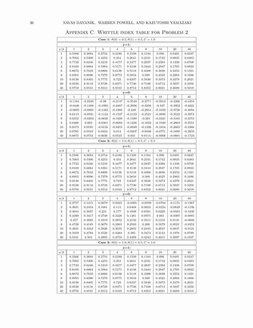
36 SAVAS DAYANIK, WARREN POWELL, AND KAZUTOSHI YAMAZAKI
Appendix C. Whittle index table for Problem 2
Case 1: θ(0) = 0.5, θ(1) = 0.5, C = 1.0
y=1:
a\b 1 2 3 4 6 8 10 20 40
1 0.5506 0.3694 0.2754 0.2186 0.1539 0.1184 0.096 0.0491 0.0247
2 0.7003 0.5306 0.4253 0.354 0.2641 0.2101 0.1742 0.0935 0.0483
3 0.7732 0.6246 0.5219 0.4477 0.3477 0.2837 0.2394 0.1338 0.0708
4 0.8169 0.6864 0.5904 0.5171 0.4138 0.3444 0.2947 0.1705 0.0922
6 0.8672 0.7633 0.6806 0.6136 0.5118 0.4388 0.3838 0.2352 0.1321
8 0.8955 0.8096 0.7379 0.6775 0.5816 0.509 0.4525 0.2903 0.1686
10 0.9138 0.8405 0.7775 0.723 0.6337 0.5636 0.5073 0.3379 0.2021
20 0.9538 0.9116 0.8728 0.8371 0.7736 0.7188 0.6712 0.5037 0.3356
40 0.9759 0.9531 0.9312 0.9103 0.8712 0.8352 0.8021 0.6689 0.5018
y=0:
a\b 1 2 3 4 6 8 10 20 40
1 -0.1184 -0.2235 -0.28 -0.3147 -0.3549 -0.3771 -0.3912 -0.4206 -0.4355
2 -0.0446 -0.1388 -0.1993 -0.2407 -0.2936 -0.3256 -0.347 -0.3952 -0.4221
3 -0.0095 -0.0905 -0.1482 -0.1906 -0.248 -0.2851 -0.3109 -0.3726 -0.4094
4 0.0113 -0.0591 -0.1124 -0.1537 -0.2123 -0.2521 -0.2806 -0.3522 -0.3974
6 0.0352 -0.0203 -0.0656 -0.1028 -0.1599 -0.201 -0.2321 -0.3165 -0.3753
8 0.0486 0.003 -0.0361 -0.0693 -0.1226 -0.1632 -0.1949 -0.2863 -0.3551
10 0.0573 0.0185 -0.0156 -0.0455 -0.0949 -0.1338 -0.1654 -0.2603 -0.3366
20 0.0765 0.0543 0.0334 0.014 -0.0207 -0.0508 -0.0771 -0.1699 -0.2633
40 0.0875 0.0753 0.0636 0.0523 0.031 0.0114 -0.0068 -0.0801 -0.1723
Case 2: θ(0) = 1.0, θ(1) = 0.5, C = 0.5
y=1:
a\b 1 2 3 4 6 8 10 20 40
1 0.5506 0.3694 0.2754 0.2186 0.1539 0.1184 0.096 0.0491 0.0247
2 0.7003 0.5306 0.4253 0.354 0.2641 0.2101 0.1742 0.0935 0.0483
3 0.7732 0.6246 0.5219 0.4477 0.3477 0.2837 0.2394 0.1338 0.0708
4 0.8169 0.6864 0.5904 0.5171 0.4138 0.3444 0.2947 0.1705 0.0922
6 0.8672 0.7633 0.6806 0.6136 0.5118 0.4388 0.3838 0.2352 0.1321
8 0.8955 0.8096 0.7379 0.6775 0.5816 0.509 0.4525 0.2903 0.1686
10 0.9138 0.8405 0.7775 0.723 0.6337 0.5636 0.5073 0.3379 0.2021
20 0.9538 0.9116 0.8728 0.8371 0.7736 0.7188 0.6712 0.5037 0.3356
40 0.9759 0.9531 0.9312 0.9103 0.8712 0.8352 0.8021 0.6689 0.5018
y=0:
a\b 1 2 3 4 6 8 10 20 40
1 0.2757 0.1415 0.0679 0.0223 -0.0305 -0.0599 -0.0784 -0.1171 -0.1367
2 0.3631 0.2453 0.1681 0.115 0.0468 0.0053 -0.0224 -0.0849 -0.1196
3 0.4044 0.3037 0.231 0.177 0.1038 0.0561 0.0229 -0.0564 -0.1036
4 0.4289 0.3417 0.2748 0.2226 0.1481 0.0975 0.061 -0.0307 -0.0885
6 0.457 0.3885 0.3319 0.2852 0.2132 0.1611 0.1216 0.0141 -0.0606
8 0.4728 0.4165 0.3679 0.3263 0.2593 0.208 0.1679 0.0521 -0.0352
10 0.4831 0.4352 0.3928 0.3555 0.2935 0.2445 0.2047 0.0847 -0.0121
20 0.5059 0.4784 0.4526 0.4284 0.385 0.3473 0.3143 0.1976 0.0799
40 0.5191 0.504 0.4895 0.4754 0.4489 0.4243 0.4015 0.3097 0.1937
Case 3: θ(0) = 1.0, θ(1) = 0.5, C = 1.0
y=1:
a\b 1 2 3 4 6 8 10 20 40
1 0.5506 0.3694 0.2754 0.2186 0.1539 0.1184 0.096 0.0491 0.0247
2 0.7003 0.5306 0.4253 0.354 0.2641 0.2101 0.1742 0.0935 0.0483
3 0.7732 0.6246 0.5219 0.4477 0.3477 0.2837 0.2394 0.1338 0.0708
4 0.8169 0.6864 0.5904 0.5171 0.4138 0.3444 0.2947 0.1705 0.0922
6 0.8672 0.7633 0.6806 0.6136 0.5118 0.4388 0.3838 0.2352 0.1321
8 0.8955 0.8096 0.7379 0.6775 0.5816 0.509 0.4525 0.2903 0.1686
10 0.9138 0.8405 0.7775 0.723 0.6337 0.5636 0.5073 0.3379 0.2021
20 0.9538 0.9116 0.8728 0.8371 0.7736 0.7188 0.6712 0.5037 0.3356
40 0.9759 0.9531 0.9312 0.9103 0.8712 0.8352 0.8021 0.6689 0.5018
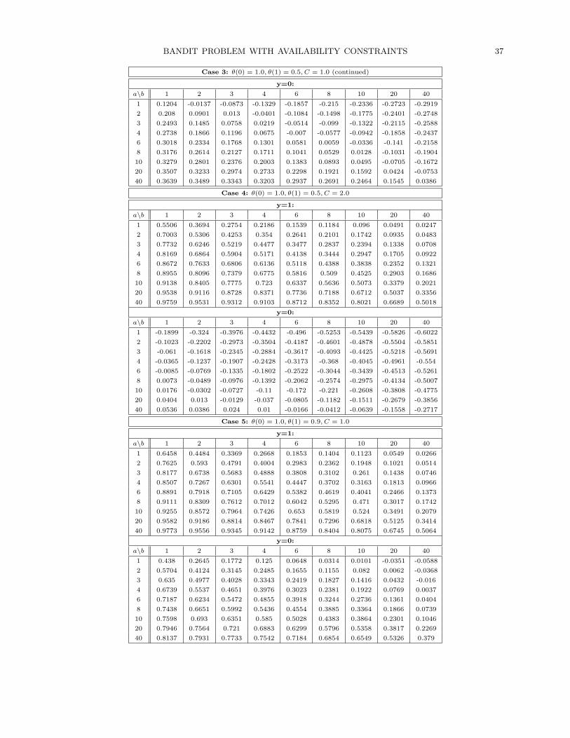
BANDIT PROBLEM WITH AVAILABILITY CONSTRAINTS 37
Case 3: θ(0) = 1.0, θ(1) = 0.5, C = 1.0 (continued)
y=0:
a\b 1 2 3 4 6 8 10 20 40
1 0.1204 -0.0137 -0.0873 -0.1329 -0.1857 -0.215 -0.2336 -0.2723 -0.2919
2 0.208 0.0901 0.013 -0.0401 -0.1084 -0.1498 -0.1775 -0.2401 -0.2748
3 0.2493 0.1485 0.0758 0.0219 -0.0514 -0.099 -0.1322 -0.2115 -0.2588
4 0.2738 0.1866 0.1196 0.0675 -0.007 -0.0577 -0.0942 -0.1858 -0.2437
6 0.3018 0.2334 0.1768 0.1301 0.0581 0.0059 -0.0336 -0.141 -0.2158
8 0.3176 0.2614 0.2127 0.1711 0.1041 0.0529 0.0128 -0.1031 -0.1904
10 0.3279 0.2801 0.2376 0.2003 0.1383 0.0893 0.0495 -0.0705 -0.1672
20 0.3507 0.3233 0.2974 0.2733 0.2298 0.1921 0.1592 0.0424 -0.0753
40 0.3639 0.3489 0.3343 0.3203 0.2937 0.2691 0.2464 0.1545 0.0386
Case 4: θ(0) = 1.0, θ(1) = 0.5, C = 2.0
y=1:
a\b 1 2 3 4 6 8 10 20 40
1 0.5506 0.3694 0.2754 0.2186 0.1539 0.1184 0.096 0.0491 0.0247
2 0.7003 0.5306 0.4253 0.354 0.2641 0.2101 0.1742 0.0935 0.0483
3 0.7732 0.6246 0.5219 0.4477 0.3477 0.2837 0.2394 0.1338 0.0708
4 0.8169 0.6864 0.5904 0.5171 0.4138 0.3444 0.2947 0.1705 0.0922
6 0.8672 0.7633 0.6806 0.6136 0.5118 0.4388 0.3838 0.2352 0.1321
8 0.8955 0.8096 0.7379 0.6775 0.5816 0.509 0.4525 0.2903 0.1686
10 0.9138 0.8405 0.7775 0.723 0.6337 0.5636 0.5073 0.3379 0.2021
20 0.9538 0.9116 0.8728 0.8371 0.7736 0.7188 0.6712 0.5037 0.3356
40 0.9759 0.9531 0.9312 0.9103 0.8712 0.8352 0.8021 0.6689 0.5018
y=0:
a\b 1 2 3 4 6 8 10 20 40
1 -0.1899 -0.324 -0.3976 -0.4432 -0.496 -0.5253 -0.5439 -0.5826 -0.6022
2 -0.1023 -0.2202 -0.2973 -0.3504 -0.4187 -0.4601 -0.4878 -0.5504 -0.5851
3 -0.061 -0.1618 -0.2345 -0.2884 -0.3617 -0.4093 -0.4425 -0.5218 -0.5691
4 -0.0365 -0.1237 -0.1907 -0.2428 -0.3173 -0.368 -0.4045 -0.4961 -0.554
6 -0.0085 -0.0769 -0.1335 -0.1802 -0.2522 -0.3044 -0.3439 -0.4513 -0.5261
8 0.0073 -0.0489 -0.0976 -0.1392 -0.2062 -0.2574 -0.2975 -0.4134 -0.5007
10 0.0176 -0.0302 -0.0727 -0.11 -0.172 -0.221 -0.2608 -0.3808 -0.4775
20 0.0404 0.013 -0.0129 -0.037 -0.0805 -0.1182 -0.1511 -0.2679 -0.3856
40 0.0536 0.0386 0.024 0.01 -0.0166 -0.0412 -0.0639 -0.1558 -0.2717
Case 5: θ(0) = 1.0, θ(1) = 0.9, C = 1.0
y=1:
a\b 1 2 3 4 6 8 10 20 40
1 0.6458 0.4484 0.3369 0.2668 0.1853 0.1404 0.1123 0.0549 0.0266
2 0.7625 0.593 0.4791 0.4004 0.2983 0.2362 0.1948 0.1021 0.0514
3 0.8177 0.6738 0.5683 0.4888 0.3808 0.3102 0.261 0.1438 0.0746
4 0.8507 0.7267 0.6301 0.5541 0.4447 0.3702 0.3163 0.1813 0.0966
6 0.8891 0.7918 0.7105 0.6429 0.5382 0.4619 0.4041 0.2466 0.1373
8 0.9111 0.8309 0.7612 0.7012 0.6042 0.5295 0.471 0.3017 0.1742
10 0.9255 0.8572 0.7964 0.7426 0.653 0.5819 0.524 0.3491 0.2079
20 0.9582 0.9186 0.8814 0.8467 0.7841 0.7296 0.6818 0.5125 0.3414
40 0.9773 0.9556 0.9345 0.9142 0.8759 0.8404 0.8075 0.6745 0.5064
y=0:
a\b 1 2 3 4 6 8 10 20 40
1 0.438 0.2645 0.1772 0.125 0.0648 0.0314 0.0101 -0.0351 -0.0588
2 0.5704 0.4124 0.3145 0.2485 0.1655 0.1155 0.082 0.0062 -0.0368
3 0.635 0.4977 0.4028 0.3343 0.2419 0.1827 0.1416 0.0432 -0.016
4 0.6739 0.5537 0.4651 0.3976 0.3023 0.2381 0.1922 0.0769 0.0037
6 0.7187 0.6234 0.5472 0.4855 0.3918 0.3244 0.2736 0.1361 0.0404
8 0.7438 0.6651 0.5992 0.5436 0.4554 0.3885 0.3364 0.1866 0.0739
10 0.7598 0.693 0.6351 0.585 0.5028 0.4383 0.3864 0.2301 0.1046
20 0.7946 0.7564 0.721 0.6883 0.6299 0.5796 0.5358 0.3817 0.2269
40 0.8137 0.7931 0.7733 0.7542 0.7184 0.6854 0.6549 0.5326 0.379
38 SAVAS DAYANIK, WARREN POWELL, AND KAZUTOSHI YAMAZAKI
References
[1] J. S. Banks and R. K. Sundaram. Denumerable-armed bandits. Econometrica, 60(5):1071–1096, 1992.
[2] J. S. Banks and R. K. Sundaram. Switching costs and the gittins index. Econometrica, 62:687–694,
1994.
[3] D. Bergemann and J. Valimaki. Efficient dynamic auctions. Cowles Foundation Discussion Paper, 1584,
2006.
[4] M. Brezzi and T. L. Lai. Incomplete learning endogenous data in dynamic allocation. Econometrica,
68(6):1511–1516, 2000.
[5] J. C. Gittins. Bandit processes and dynamic allocation indices. J. Roy. Statist. Soc. Ser. B, 41(2):148–
177, 1979. With discussion.
[6] K. D. Glazebrook, P. S. Ansell, R. T. Dunn, and R. R. Lumley. On the optimal allocation of service to
impatient tasks. J. Appl. Probab., 41(1):51–72, 2004.
[7] K. D. Glazebrook and H. M. Mitchell. An index policy for a stochastic scheduling model with improv-
ing/deteriorating jobs. Naval Res. Logist., 49(7):706–721, 2002.
[8] K. D. Glazebrook, J. Nino-Mora, and P. S. Ansell. Index policies for a class of discounted restless
bandits. Adv. in Appl. Probab., 34(4):754–774, 2002.
[9] K. D. Glazebrook, D. Ruiz-Hernandez, and C. Kirkbride. Some indexable families of restless bandit
problems. Adv. in Appl. Probab., 38(3):643–672, 2006.
[10] B. Jovanovic. Job matching and the theory of turnover. The Journal of Political Ecoomy, 87, Part
1.(5):972–990, 1979.
[11] T. Jun. A survey on the bandit problem with switching costs. De Economist, 1524(4):513–541, 2004.
[12] M. N. Katehakis and C. Derman. Computing optimal sequential allocation rules in clinical trials. In
Adaptive statistical procedures and related topics (Upton, N.Y., 1985), volume 8 of IMS Lecture Notes
Monogr. Ser., pages 29–39. Inst. Math. Statist., Hayward, CA, 1986.
[13] M. N. Katehakis and A. F. Veinott, Jr. The multi-armed bandit problem: decomposition and compu-
tation. Math. Oper. Res., 12(2):262–268, 1987.
[14] R. A. Miller. Job matching and occupational choice. The Journal of Political Economy, 926(6):1086–
1120, 1984.
[15] J. Nino-Mora. Restless bandits, partial conservation laws and indexability. Adv. in Appl. Probab.,
33(1):76–98, 2001.
[16] C. H. Papadimitriou and J. N. Tsitsiklis. The complexity of optimal queuing network control. Math.
Oper. Res., 24(2):293–305, 1999.
[17] S. Ross. Introduction to Stochastic Dynamic Programming. Academic Press, INC., 1983.
[18] M. Rothschild. A two-armed bandit theory of market pricing. J. Econom. Theory, 9(2):185–202, 1974.
[19] J. N. Tsitsiklis. A short proof of the Gittins index theorem. Ann. Appl. Probab., 4(1):194–199, 1994.
[20] R. R. Weber and G. Weiss. On an index policy for restless bandits. J. Appl. Probab., 27(3):637–648,
1990.
[21] R. R. Weber and G. Weiss. Addendum to: “On an index policy for restless bandits”. Adv. in Appl.
Probab., 23(2):429–430, 1991.
[22] P. Whittle. Multi-armed bandits and the Gittins index. J. Roy. Statist. Soc. Ser. B, 42(2):143–149,
1980.
BANDIT PROBLEM WITH AVAILABILITY CONSTRAINTS 39
[23] P. Whittle. Restless bandits: activity allocation in a changing world. J. Appl. Probab., (Special Vol.
25A):287–298, 1988. A celebration of applied probability.
Department of Operations Research and Financial Engineering, Princeton University,
New Jersey
E-mail address, Savas Dayanik: [email protected]
E-mail address, Warren Powell: [email protected]
E-mail address, Kazutoshi Yamazaki: [email protected]