availability models in practice

&CHAPTER 11

Availability Modeling in Practice

KISHOR S. TRIVEDI,1 ARCHANA SATHAYE,2 and SRINIVASAN RAMANI3

1Dept. of Electrical and Computer Engineering, Duke University, Durham, NC 27708-0291

(E-mail: [email protected]); 2Dept. of Computer Science, San Jose State University, San Jose,

CA 95192 (E-mail: [email protected]); 3IBM Corporation, 3039 Cornwallis Rd., RTP,

NC 27709 (E-mail: [email protected]).

As computer systems continue to be applied to mission-critical environments,

techniques to evaluate their dependability become more and more important.

Of the dependability measures used to characterize a system, availability is one of

the most important.

Techniques to evaluate a system’s availability can be broadly categorized as

measurement-based and model-based. Measurement-based evaluation is expensive

because it requires building a real system and taking measurements and then analyz-

ing the data statistically. Model-based evaluation on the other hand is inexpensive

and relatively easier to perform. In Chapter 11, we first look at some availability

modeling techniques and take up a case study from an industrial setting to illustrate

the application of the techniques to a real problem. Although easier to perform,

model-based availability analysis poses problems like largeness and complexity

of the models developed, which makes the models difficult to solve. Chapter 11

also illustrates several techniques to deal with largeness and complexity issues.

11.1 INTRODUCTION

Complex computer systems are widely used in different applications, ranging from

flight control, and command and control systems to commercial systems like infor-

mation and financial services. These applications demand high performance and

high availability. Availability evaluation addresses failure and recovery aspects of

a system, whereas performance evaluation addresses processing aspects and

assumes that the system components do not fail. For gracefully degrading systems,

a measure that combines system performance and availability aspects is more

293

Dependable Computing Systems. Edited by Hassan B. Diab and Albert Y. ZomayaISBN 0-471-67422-2 Copyright # 2005 John Wiley & Sons, Inc.

meaningful than separate measures of performance and availability. These

composite measures are called performability measures. The two basic approaches

to evaluate the availability/performance measures of a system are as follows:

measurement-based and model-based. In measurement-based evaluation, the

required measures are estimated from measured data using statistical inference tech-

niques. The data are measured from a real system or its prototype. In case of avail-

ability evaluation, measurements are not always feasible. The reason being either

the system has not been built yet or it is too expensive to conduct experiments.

That is, in a high availability system one would need to measure data from several

systems to gather good sample data. On the other hand, injecting faults in a system

can be an expensive procedure. Model-based evaluation is the cost-effective sol-

ution because it allows system evaluation without having to build and measure a

system. In this chapter, we discuss availability modeling techniques and their

usage in practice. To emphasize the practicality of these techniques, we discuss

their pros and cons with respect to a case study, VAXcluster systems1 of Digital

Equipment Corporation (DEC2).

We first discuss different availability modeling approaches in Section 11.2. In

Section 11.3, we discuss the benefits of utilizing a composite availability and per-

formance model in practice instead of a pure availability model. Our discussion

emphasizes this point using a model developed for multiprocessors to determine

the optimal number of processors in the system. In Section 11.4, we present a

case study to demonstrate the utility of availability modeling in a corporate

environment.

11.2 MODELING APPROACHES

Model-based evaluation can be through discrete-event simulation or analytical

models or hybrid models combining simulation and analytical methods. A discrete-

event simulation model can depict detailed system behavior, as it is essentially a

program whose execution simulates the dynamic behavior of the system and

evaluates the required measures. An analytical model consists of a set of equations

describing the system behavior. The required measures are obtained by solving these

equations. In simple cases, closed-form solutions are obtained, but more frequently

numerical solutions of the equations are necessary.

The main benefit of discrete-event simulation is the ability to depict detailed

system behavior in the models. Also, the flexibility of discrete-event simulation

allows its use in performance, availability, and performability modeling. The

main drawback of discrete-event simulation is the long execution time, particularly

when tight confidence bounds are required in the solutions obtained. Also, carrying

out a “what if” analysis requires rerunning the model for different input parameters.

Advances in simulation speed-up techniques, such as regenerative simulation,

1Later known as TruClusters.2Now part of Hewlett-Packard Company.

294 AVAILABILITY MODELING IN PRACTICE

importance sampling [27], importance splitting [26], and parallel and distributed

simulation, also need to be considered.

Analytical models [7] are more of an abstraction of the real system than

discrete-event simulation models. In general, analytical models tend to be easier

to develop and faster to solve than a simulation model. The main drawback is the

set of assumptions that are often necessary to make analytical models tractable.

Recent advances in model generation and solution techniques as well as computing

power make analytical models more attractive. In this chapter, we discuss model-

based evaluation using analytical techniques and how one can achieve results that

are useful in practice.

11.2.1 Analytical Availability Modeling Approaches

A system modeler can either choose state space or non-state space analytical

modeling techniques. The choice of an appropriate modeling technique to represent

the system behavior is dictated by factors such as the measures of interest, level

of detailed system behavior to be represented and the capability of the model to

represent it, ease of construction, and availability of software tools to specify and

solve the model. In this section, we discuss several non-state space and state

space modeling techniques.

11.2.2 Non-state Space Models

Non-state space models can be solved without generating the underlying state space.

Practically speaking, these models can be easily used for solving systems with

hundreds of components because there are many relatively good algorithms

available for solving such models [22]. Non-state space models can be solved to

compute measures like system availability, reliability, and system mean time to fail-

ure (MTTF). The two main assumptions used by the efficient solution techniques are

statistically independent failures and independent repair units for components. The

non-state space model types used to evaluate system availability are “reliability

block diagrams” and “fault trees.” In gracefully degradable systems, knowledge

of the performance of the system is also essential. Non-state space model types

used to evaluate system performance are “product-form queuing models” and

“task-precedence graphs” [16].

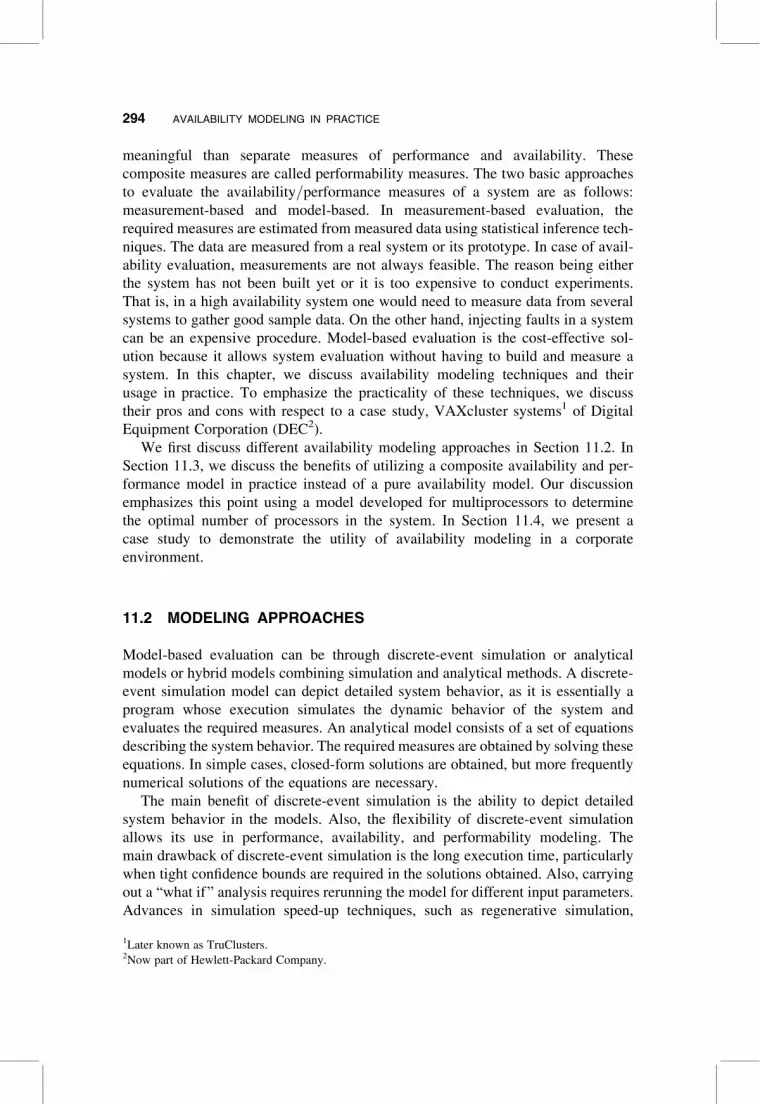
11.2.2.1 Reliability Block Diagram In a reliability block diagram (RBD),

each component of the system is represented as a block [16, 25]. This representation

of the system as a collection of components is done at the level of granularity that

is appropriate for the measurements to be obtained. The blocks are then connected

in series and/or in parallel based on the operational dependency between the

components. If for the system to be up, every component of a set of components

needs to be operational, then those blocks are connected in series in the RBD. On

the other hand, if the system can survive with at least one component, then those

blocks are connected in parallel. An RBD can be used to easily compute availability

if the repair times (and failure times) are all independent. Figure 11.1(a) shows

11.2 MODELING APPROACHES 295

an RBD representing a multiprocessor availability model with n processors where

at least one processor is required for the system to be up. This RBD represents a

simple parallel system. Given a failure rate g and repair rate t (for the purpose of

illustration, consider identical failure and repair rates for all processors), the

availability of processor Proci is given by,

A ¼t

gþ t: (11:1)

The availability of the parallel system is then given by [16],

A ¼ 1 �Yn

i¼1

(1 � Ai) ¼ 1 �

g

gþ t

� �n

: (11:2)

11.2.2.2 Fault Trees A fault tree [16], like a RBD, is useful for availability

analysis. It is a pictorial representation of the sequence of events/conditions to be

satisfied for a failure to occur. A fault tree uses and, or and k of n gates to represent

this combination of events in a tree-like structure. To represent situations where one

failure event propagates failure along multiple paths in the fault tree, fault trees can

have repeated nodes. Several efficient algorithms for solving fault trees exist. These

include algorithms for fault trees without repeated components [11], a multiple vari-

able inversion (MVI) algorithm called the LT algorithm to obtain sum of disjoint

products (SDP) from mincut set [15], and the factoring/conditioning algorithm

that works by factoring a fault tree with repeated nodes into a set of fault trees with-

out repeated nodes [19]. Binary decision diagram (BDD)-based algorithms can be

used to solve very large fault trees [5, 6, 22, 28]. Figure 11.1(b) shows the fault

tree model for our multiprocessor system. UAi represents the unavailability of

processor i. The and gate indicates that the multiprocessor system fails when all

the n processors becomes unavailable. The output of the top gate of the fault tree

represents failure of the multiprocessor system.

.

.

.

Proc 1A1

(a)(b)

Proc 2A2

Proc nAn

. . .

UA1 UA2 UAn

FAILURE

Figure 11.1 A multiprocessor system (a) Reliability block diagram, (b) Fault tree.


11.2.3 State Space Models

RBDs and fault trees cannot easily handle more complex situations such as failure/repair dependencies and shared repair facilities. In such cases, more detailed models

such as state space models are required. Here, we discuss some Markovian state

space models [3, 25].

11.2.3.1 Markov Chains In this section, we consider homogeneous Markov

chains. A homogeneous continuous time Markov chain (CTMC) [25] is a state

space model, in which each state represents various conditions of the system. In

homogeneous CTMCs, transitions from one state to another occur after a time

that is exponentially distributed. The arcs representing a transition from one state

to another are labeled by the constant rate corresponding to the exponentially

distributed time of the transition. If a state in the CTMC has no transitions leaving

it, then that state is called an absorbing state, and a CTMC with one or more such

states is said to be an absorbing CTMC. For the multiprocessor example, we now

illustrate how a Markov chain can be developed to capture shared repair and

multiple failure modes.

The parameters associated with a system availability model that we will now

develop for our multiprocessor system are the failure rate g of each processor and

the processor repair rate t. The processor fault is covered with probability c and

not covered with probability 1–c. After a covered fault, the system is up in a

degraded mode after a reconfiguration delay. On the other hand, an uncovered

fault is followed by a longer delay imposed by a reboot action. The reconfiguration

and reboot delays are assumed to be exponentially distributed with means 1/d and

1/b, respectively. In practice, the reconfiguration and reboot times are extremely

small compared with the times between failures and repairs; hence, we assume

that failures and repairs do not occur during these actions. System availability can

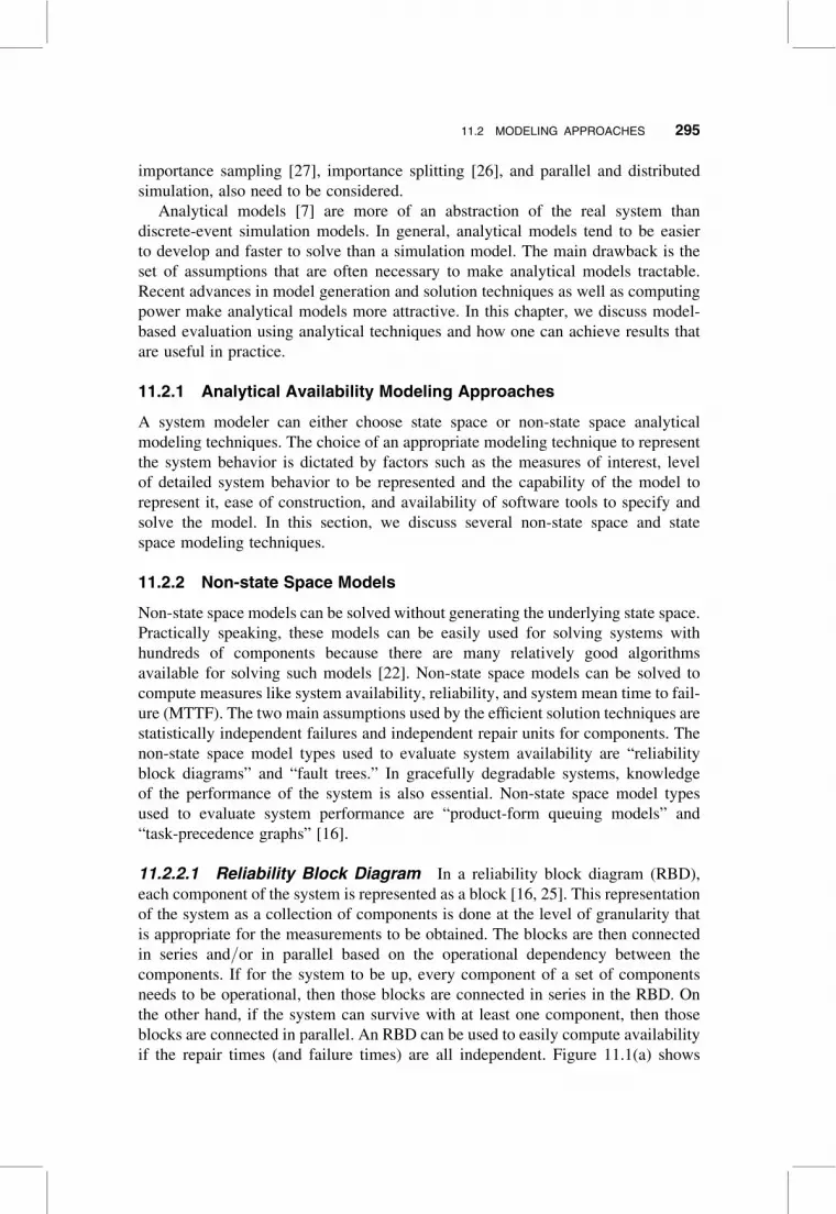
be modeled using the Markov chain shown in Fig. 11.2.

For the system to be up, at least one processor out of the n processors needs

to be operational. The state i, 1 � i � n in the Markov model represents that i pro-

cessors are operational and that n 2 i processors are waiting for on-line repair. The

states Xn2i and Yn2i , for i ¼ 0, . . . , n 2 2, represent that a system is undergoing a

reconfiguration and is being rebooted, respectively. The steady-state probabilities

1 0n-2n-1n

n c

(1-c)

τ

β

δ (n-1)γ

γn

γ c

(n-1) γ (1-c)

τ

β

δ γ

τ

Xn

Yn

Xn-1

Yn-1

. . .

Figure 11.2 Multiprocessor Markov chain model.


pi for each state i can be computed as [24, 25]

pn�i ¼n!

(n � i)!

g

t

� �i

pn, i ¼ 1, 2, . . . , n

pXn�i¼

n!

(n � i)!

g(n � i)c

d

g

t

� �i

pn, i ¼ 0,1, . . . ; n � 2 (11:3)

pYn�i¼

n!

(n � i)!

g(n � i)(1 � c)

b

g

t

� �i

pn, i ¼ 0,1, . . . ; n � 2,

where

pn ¼Xn

i¼0

g

t

� �i n!

(n � i)!þXn�2

i¼0

g

t

� �i g(n � i)cn!

d(n � i)!

"

þXn�2

i¼0

g

t

� �i g(n � i)(1 � c)n!

b(n � i)!

#�1

: (11:4)

The steady state availability, A(n), can be written as,

A(n) ¼Xn�1

i¼0

pn�i ¼

Pn�1i¼0 u i=(n � i)!

Q1

, (11:5)

where u ¼ g/t and

Q1 ¼Xn

i¼0

u i

(n � i)!þXn�2

i¼0

g(n � i)u i

(n � i)!

c

dþ

(1 � c)

b

� �: (11:6)

Then the system unavailability defined as a function of n is given by,

UA(n) ¼ 1 �Pn

i¼1 pi.

11.2.3.2 Markov Reward Models A Markov reward model (MRM) is essen-

tially a Markov chain with “reward rates” ri associated with each state i. This makes

specification of measures of interest more convenient. We can now denote the

reward rate of the CTMC at time t as

Z(t) ¼ rX(t): (11:7)

The expected steady-state reward rate for an irreducible CTMC can be written as

E½Z� ¼ limt!1

E½Z(t)� ¼X

i

ripi: (11:8)


By appropriately choosing reward rates (or weights) for each state, the appropriate

measure can be obtained for the model on hand. For example, for the multiprocessor

example of Fig. 11.2, if the reward rates are defined as ri ¼ 1 for states i ¼ 1, . . . , n

and ri ¼ 0; otherwise, the expected steady-state reward rate gives the steady-state

availability.

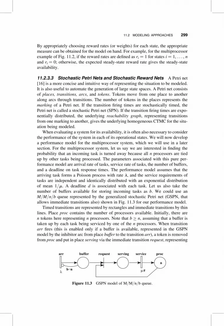
11.2.3.3 Stochastic Petri Nets and Stochastic Reward Nets A Petri net

[16] is a more concise and intuitive way of representing the situation to be modeled.

It is also useful to automate the generation of large state spaces. A Petri net consists

of places, transitions, arcs, and tokens. Tokens move from one place to another

along arcs through transitions. The number of tokens in the places represents the

marking of a Petri net. If the transition firing times are stochastically timed, the

Petri net is called a stochastic Petri net (SPN). If the transition firing times are expo-

nentially distributed, the underlying reachability graph, representing transitions

from one marking to another, gives the underlying homogeneous CTMC for the situ-

ation being modeled.

When evaluating a system for its availability, it is often also necessary to consider

the performance of the system in each of its operational states. We will now develop

a performance model for the multiprocessor system, which we will use in a later

section. For the multiprocessor system, let us say we are interested in finding the

probability that an incoming task is turned away because all n processors are tied

up by other tasks being processed. The parameters associated with this pure per-

formance model are arrival rate of tasks, service rate of tasks, the number of buffers,

and a deadline on task response times. The performance model assumes that the

arriving task forms a Poisson process with rate l, and the service requirements of

tasks are independent and identically distributed with an exponential distribution

of mean 1/m. A deadline d is associated with each task. Let us also take the

number of buffers available for storing incoming tasks as b. We could use an

M/M/n/b queue represented by the generalized stochastic Petri net (GSPN, that

allows immediate transitions also) shown in Fig. 11.3 for our performance model.

Timed transitions are represented by rectangles and immediate transitions by thin

lines. Place proc contains the number of processors available. Initially, there are

n tokens here representing n processors. Note that b � n, assuming that a buffer is

taken up by each task being serviced by one of the n processors. When transition

arr fires (this is enabled only if a buffer is available, represented in the GSPN

model by the inhibitor arc from place buffer to the transition arr), a token is removed

from proc and put in place serving via the immediate transition request, representing

arr

b−n

buffer request serving service proc

n

λ µ #

Figure 11.3 GSPN model of M/M/n/b queue.


one less free processor. At the same time that this happens, a token is also removed

from place buffer, to denote that the task is not waiting. The immediate transition

request will be enabled if there is at least one token in both place proc and place

buffer. This enforces the condition that, when a task arrives, a processor must be

available. If not, the task waits, represented by the retention of the token in place

buffer. If there are more arrivals when all processors are busy, the buffers start to

fill up. Transition arr is disabled (indicated by the inhibitor arc from place buffer)

when there are b 2 n tokens in place buffer, since there can only be b tasks in the

system: n in place serving that are currently being serviced and b 2 n in place

buffer. Therefore, the probability that an incoming task is rejected is the probability

that transition arr is disabled. Transition service represents the service time for each

task and has a firing rate that depends on the number of tokens in place serving (indi-

cated by the notation m#). That is, if place serving has p tokens, transition service has

a firing rate of pm. The expectation of the firing rate of transition service at steady

state gives the throughput of the multiprocessor system. Several tools such as SPNP

[4] are available for solving stochastic Petri net and stochastic reward net models.

In practical system design, a pure availability model may not be enough for

systems such as gracefully degradable ones. In conjunction with availability, the

performance of the system as it degrades needs to be considered. This requires

a “performability” model [12, 21] that includes both performance and availability

measures. In the next section, we present an example of a system for which a

performability measure is needed.

11.3 COMPOSITE AVAILABILITY AND PERFORMANCE MODEL

Consider the multiprocessor system again but with varying number of processors, n,

each with the same capacity. A key question asked in practice is regarding the

number of processors needed (sizing). As we discuss below, the optimal configur-

ation in terms of the number of processors is a function of the chosen measure of

system effectiveness [24]. We begin our sizing based on measures from a “pure”

availability model. Next, we consider sizing based on system performance

measures. Last, we consider a composite of performance and availability measures

to capture the effect of system degradation.

11.3.1 Multiprocessor Sizing Based on Availability

A CTMC model for the failure/repair characteristics of the multiprocessor system is

shown in Fig. 11.2. The details of the model were discussed in the introduction to

Markov chains in the previous section. The downtime during an observation interval

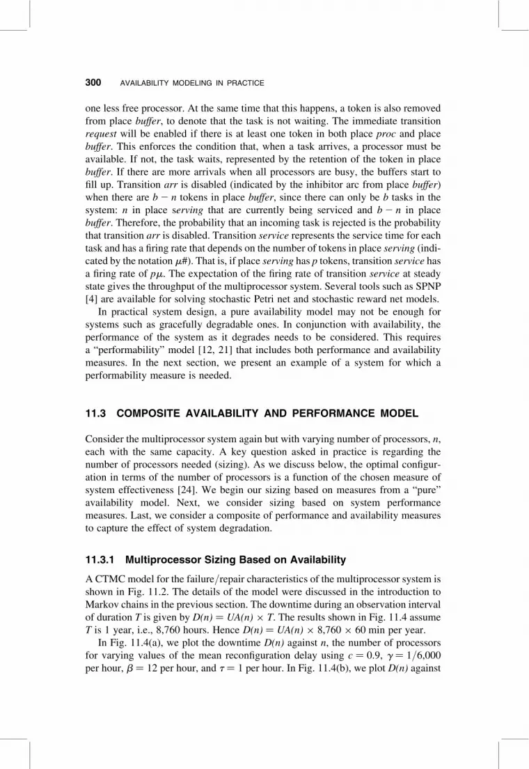
of duration T is given by D(n) ¼ UA(n) � T. The results shown in Fig. 11.4 assume

T is 1 year, i.e., 8,760 hours. Hence D(n) ¼ UA(n) � 8,760 � 60 min per year.

In Fig. 11.4(a), we plot the downtime D(n) against n, the number of processors

for varying values of the mean reconfiguration delay using c ¼ 0.9, g ¼ 1/6,000

per hour, b ¼ 12 per hour, and t ¼ 1 per hour. In Fig. 11.4(b), we plot D(n) against


n for different coverage values with a mean reconfiguration delay, d ¼ 10 seconds.

We conclude from these results that the availability benefits of multiprocessing (i.e.,

increase in availability with increase in the number of operational processors) is

possible only if the coverage is near perfect and the reconfiguration delay is very

small or most of the other processors are able to carry out useful work while a

fault is being handled. We further observe that, for most practical parameter

values, the optimal number of processors is 2 or 3. As the number of processors

increases beyond 2, the downtime is mainly due to reconfigurations. Also, the

number of reconfigurations increases almost linearly with the number of processors.

1

10

100

1000

1 2 3 4 5 6 7 8

Dow

ntim

e in

min

s per

yea

r

Number of processors

Mean Reconfiguration Delay = 1 secMean Reconfiguration Delay = 10 secMean Reconfiguration Delay = 30 sec

1 2 3 4 5 6 7 810

-1

101

100

102


Dow

ntim

e in

min

utes

per

yea

r

Coverage = 0.9 Coverage = 0.95Coverage = 0.99

(b)

(a)

Figure 11.4 Downtime Vs. Number of processors for—(a) different mean reconfiguration

delays, (b) different coverage values.

11.3 COMPOSITE AVAILABILITY AND PERFORMANCE MODEL 301

In the next subsection, we consider a performance-based model for the multi-

processor sizing problem.

11.3.2 Multiprocessor Sizing Based on Performance

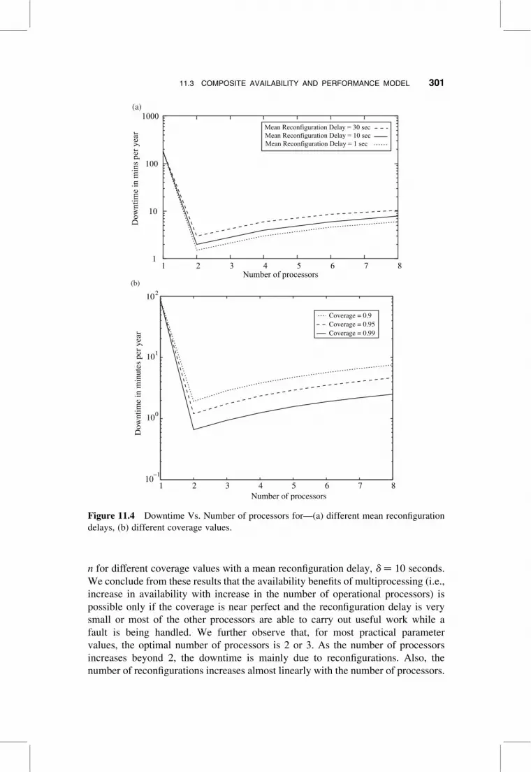
On the lines of the GSPN example discussed in Section 11.2.3, we use an M/M/n/b

queuing model with finite buffer capacity to compute the probability that a task is

rejected because the buffer is full. In Fig. 11.3, this is the probability that transition

arr is disabled. In Fig. 11.5, we plot the loss probability as a function of n for differ-

ent values of arrival rates.

We observe that the loss probability reduces as the number of processors

increases. The conclusion from the performance model of the fault-free system is

that the system improves as the number of processors is increased. The details of

this model and results have been previously presented [24].

The above models point out the deficiency of simply considering a pure avail-

ability or performance measure. The pure availability measure ignores different

levels of performance at various system states, whereas the pure performance

measure ignores the failure/repair behavior of the system. The next section

considers combined measures of performance and availability.

11.3.3 Multiprocessor Sizing Based on Performance and Availability

Different levels of performance can be taken into account by attaching a reward rate

ri corresponding to some measure of performance to each state i of the failure/repair

Markov model in Fig. 11.2. The resulting Markov reward model can then be

analyzed for various combined measures of performance and availability. The sim-

plest reward rate assignment is to let ri ¼ i for states with i operational processors

0.3

0.4

0.5

0.6

0.7

0.8

0.9

1

1 2 3 4 5 6 7 8

ytilibaborp ssoL


Arrival Rate = 1/secArrival Rate = 80/secArrival Rate = 180/sec

Figure 11.5 Loss probability Vs. Number of processors.


and ri ¼ 0 for down states. With this reward assignment, shown in Table 11.1, we

can compute the capacity-oriented availability, COA(n) as the expected reward

rate in the steady state. This can be written as COA(n) ¼Pn

i¼1 ipi. COA(n) is an

upper bound on system performance that equates performance with system capacity.

Next, let us consider a performance-oriented reward rate assignment.

When i processors are operational, we can use an M/M/i/b queuing model (such

as the GSPN in Fig. 11.3) to describe the performance of the multiprocessor system.

We then assign a reward rate of ri ¼ 0 for each down state i, for all other states, we

assign a reward rate of ri ¼ Tb(i), which is the throughput for a system with i

processors and b buffers (see Table 11.2).

With this assignment, the expected reward rate at steady state computes the

throughput-oriented availability, TOA(n), which can be written as, TOA(n) ¼Pni¼1 Tb(i)pi. In Fig. 11.6, we plot COA(n) and TOA(n) for different values of the

arrival rate l.

These two measures show that in order to process a heavier workload more than

two processors are needed. The measures COA and TOA are not adequate measures

of system effectiveness because they obliterate the effects of failure/repair and

merely show the effects of system capacity and the load. Previously [24], a measure

of system effectiveness, total loss probability, was proposed that “equally” reflected

fault-free behavior and behavior in the presence of faults. The total loss probability

is defined as the sum of rejection probability due to the system being down or

full and the probability of a response time deadline being violated. The total loss

probability is computed by using the following reward rate assignments (also

shown in Table 11.3):

ri ¼1, if i is a down state,

qb(i) þ ½1 � qb(i)�½P(Rb(i) . d)�, if i is an operational state:

�

TABLE 11.1 Reward Rates for COA.

State Reward Rate, ri

0 0

1 � i � n i

Xn2i and Yn2i; i ¼ 0, . . . , n 2 2 0

TABLE 11.2 Reward Rates for TOA.


0 0

1 � i � n Tb(i), throughput of system with

i processors and b buffers

Xn2i and Yn2i; i ¼ 0, . . . , n 2 2 0

11.3 COMPOSITE AVAILABILITY AND PERFORMANCE MODEL 303

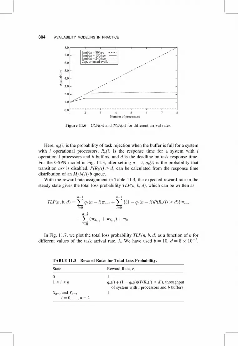
Here, qb(i) is the probability of task rejection when the buffer is full for a system

with i operational processors, Rb(i) is the response time for a system with i

operational processors and b buffers, and d is the deadline on task response time.

For the GSPN model in Fig. 11.3, after setting n ¼ i, qb(i) is the probability that

transition arr is disabled. P(Rb(i) . d) can be calculated from the response time

distribution of an M/M/i/b queue.

With the reward rate assignment in Table 11.3, the expected reward rate in the

steady state gives the total loss probability TLP(n, b, d), which can be written as

TLP(n, b, d) ¼Xn�1

i¼0

qb(n � i)pn�i þXn�1

i¼0

{(1 � qb(n � i))P(Rb(i) . d)}pn�i

þXn�2

i¼0

(pXn�iþ pYn�i

) þ p0:

In Fig. 11.7, we plot the total loss probability TLP(n, b, d) as a function of n for

different values of the task arrival rate, l. We have used b ¼ 10, d ¼ 8 � 1025,

0.0

1.0

2.0

3.0

4.0

5.0

6.0

7.0

8.0

1 2 3 4 5 6 7 8

Ava

ilabi

lity


lambda = 80/seclambda = 150/seclambda = 240/secCap. oriented avail.

Figure 11.6 COA(n) and TOA(n) for different arrival rates.

TABLE 11.3 Reward Rates for Total Loss Probability.


0 1

1 � i � n qb(i) þ (1 2 qb(i))(P(Rb(i) . d)), throughput

of system with i processors and b buffers

Xn2i and Yn2i

i ¼ 0, . . . , n 2 2

1


and m ¼ 100 per second. We see that, as the value of l increases, the optimal

number of processors, n�, increases as well. For instance, n� ¼ 4 for l ¼ 20,

n� ¼ 5 for l ¼ 40, n� ¼ 6 for l ¼ 60. (Note that n� ¼ 2 for l ¼ 0 from

Fig. 11.4.) The model can be used to show that the optimal number of processors

increases with the task arrival rate, tighter deadlines, and smaller buffer spaces.

11.4 DIGITAL EQUIPMENT CORPORATION CASE STUDY

In this section, we discuss a case study to demonstrate that, in practice, the choice of

an appropriate model type is dictated by the availability measures of interest, the

level of detailed system behavior to be represented, ease of model specification

and solution, representation power of the model type selected, and access to suitable

tools or toolkits that can automate model specification and solution.

In particular we describe the availability models for Digital Equipment Corpor-

ation’s (DEC) VAXcluster system. VAXclusters are used in different application

environments; hence, several availability, reliability, and performability measures

need to be computed. VAXclusters used as commercial computer systems in a

general data processing environment require us to evaluate system availability

and performability measures. To consider VAXclusters in highly critical appli-

cations, such as life support systems and financial data processing systems, we

evaluate many system reliability measures. These two measures were not adequate

for some financial institution customers of VAXclusters. We therefore evaluated

1 2 3 4 5 6 7 80.9964

0.9966

0.9968

0.997

0.9972

0.9974

0.9976

0.9978

0.998

0.9982

0.9984


Tota

l los

s pr

obab

ility

λ = 20λ = 40λ = 60

Figure 11.7 Total loss probability Vs. number of processors for different task arrival rates.

11.4 DIGITAL EQUIPMENT CORPORATION CASE STUDY 305

task completion measures to compute probability of application interruption during

its execution period.

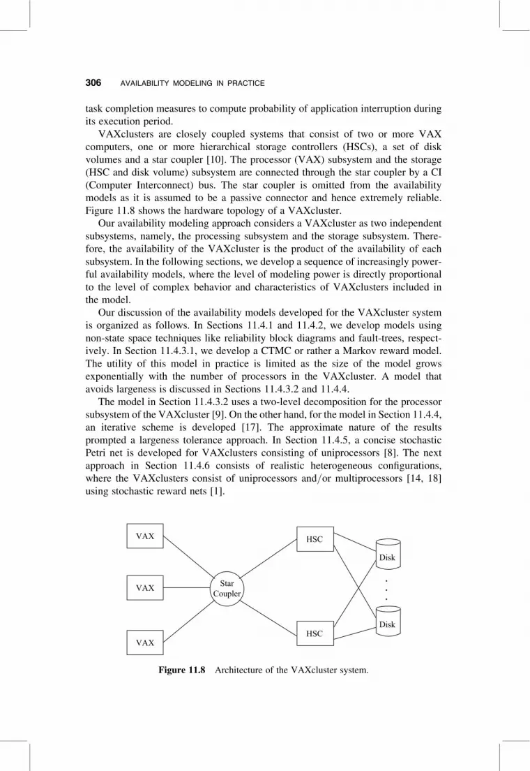
VAXclusters are closely coupled systems that consist of two or more VAX

computers, one or more hierarchical storage controllers (HSCs), a set of disk

volumes and a star coupler [10]. The processor (VAX) subsystem and the storage

(HSC and disk volume) subsystem are connected through the star coupler by a CI

(Computer Interconnect) bus. The star coupler is omitted from the availability

models as it is assumed to be a passive connector and hence extremely reliable.

Figure 11.8 shows the hardware topology of a VAXcluster.

Our availability modeling approach considers a VAXcluster as two independent

subsystems, namely, the processing subsystem and the storage subsystem. There-

fore, the availability of the VAXcluster is the product of the availability of each

subsystem. In the following sections, we develop a sequence of increasingly power-

ful availability models, where the level of modeling power is directly proportional

to the level of complex behavior and characteristics of VAXclusters included in

the model.

Our discussion of the availability models developed for the VAXcluster system

is organized as follows. In Sections 11.4.1 and 11.4.2, we develop models using

non-state space techniques like reliability block diagrams and fault-trees, respect-

ively. In Section 11.4.3.1, we develop a CTMC or rather a Markov reward model.

The utility of this model in practice is limited as the size of the model grows

exponentially with the number of processors in the VAXcluster. A model that

avoids largeness is discussed in Sections 11.4.3.2 and 11.4.4.

The model in Section 11.4.3.2 uses a two-level decomposition for the processor

subsystem of the VAXcluster [9]. On the other hand, for the model in Section 11.4.4,

an iterative scheme is developed [17]. The approximate nature of the results

prompted a largeness tolerance approach. In Section 11.4.5, a concise stochastic

Petri net is developed for VAXclusters consisting of uniprocessors [8]. The next

approach in Section 11.4.6 consists of realistic heterogeneous configurations,

where the VAXclusters consist of uniprocessors and/or multiprocessors [14, 18]

using stochastic reward nets [1].

.

.

.StarCoupler

VAX

VAX

VAX

HSC

HSC

Disk

Disk

Figure 11.8 Architecture of the VAXcluster system.


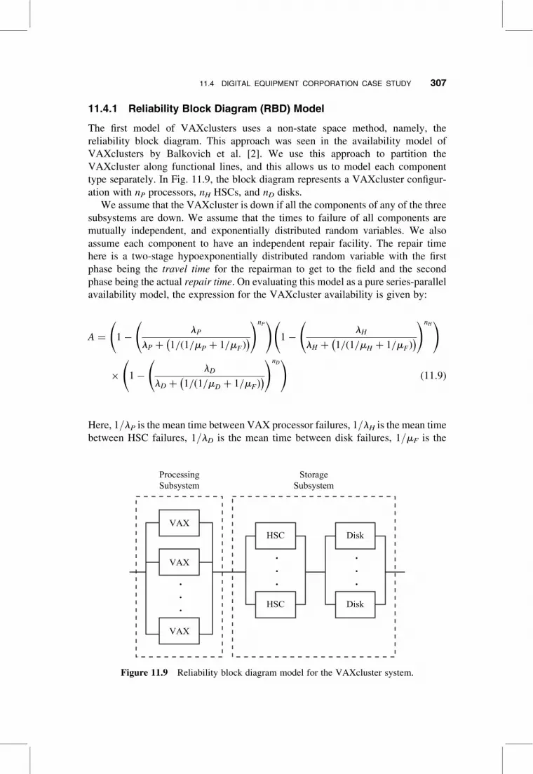
11.4.1 Reliability Block Diagram (RBD) Model

The first model of VAXclusters uses a non-state space method, namely, the

reliability block diagram. This approach was seen in the availability model of

VAXclusters by Balkovich et al. [2]. We use this approach to partition the

VAXcluster along functional lines, and this allows us to model each component

type separately. In Fig. 11.9, the block diagram represents a VAXcluster configur-

ation with nP processors, nH HSCs, and nD disks.

We assume that the VAXcluster is down if all the components of any of the three

subsystems are down. We assume that the times to failure of all components are

mutually independent, and exponentially distributed random variables. We also

assume each component to have an independent repair facility. The repair time

here is a two-stage hypoexponentially distributed random variable with the first

phase being the travel time for the repairman to get to the field and the second

phase being the actual repair time. On evaluating this model as a pure series-parallel

availability model, the expression for the VAXcluster availability is given by:

A ¼ 1 �lP

lP þ 1=(1=mP þ 1=mF)� �

!nP !

1 �lH

lH þ 1=(1=mH þ 1=mF)� �

!nH !

� 1 �lD

lD þ 1=ð1=mD þ 1=mFÞ� �

!nD !

(11:9)

Here, 1/lP is the mean time between VAX processor failures, 1/lH is the mean time

between HSC failures, 1/lD is the mean time between disk failures, 1/mF is the

.

.

.

.

.

.

.

.

.

VAX

VAX

VAX

HSC

HSC

Disk

Disk

ProcessingSubsystem

StorageSubsystem

Figure 11.9 Reliability block diagram model for the VAXcluster system.


mean field service travel time, and 1/mP, 1/mH , and 1/mD are the mean time to

repair a VAX processor, HSC, and disk, respectively.

The assumption that a VAXcluster is down when all the components of any of

the three subsystems are down is not in tune with reality. For a VAXcluster to be

operational, the system should meet quorum, where quorum is the minimum

number of VAXs required for the VAXcluster to function.

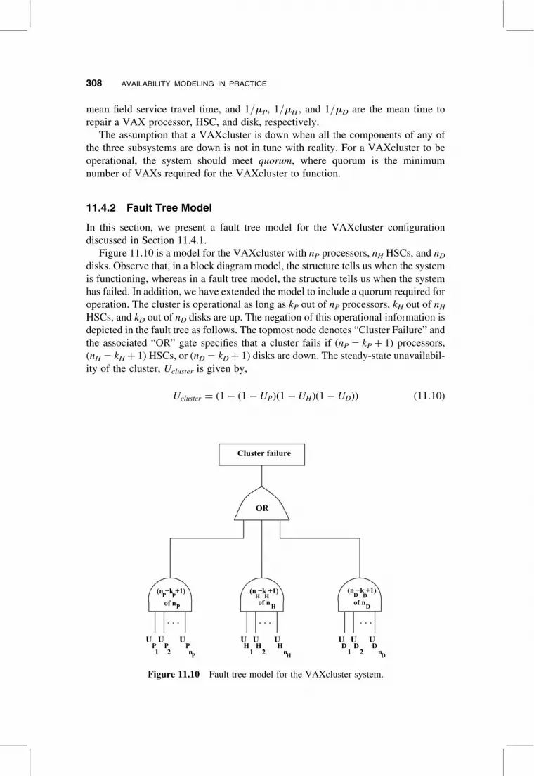
11.4.2 Fault Tree Model

In this section, we present a fault tree model for the VAXcluster configuration

discussed in Section 11.4.1.

Figure 11.10 is a model for the VAXcluster with nP processors, nH HSCs, and nD

disks. Observe that, in a block diagram model, the structure tells us when the system

is functioning, whereas in a fault tree model, the structure tells us when the system

has failed. In addition, we have extended the model to include a quorum required for

operation. The cluster is operational as long as kP out of nP processors, kH out of nH

HSCs, and kD out of nD disks are up. The negation of this operational information is

depicted in the fault tree as follows. The topmost node denotes “Cluster Failure” and

the associated “OR” gate specifies that a cluster fails if (nP 2 kP þ 1) processors,

(nH 2 kH þ 1) HSCs, or (nD 2 kD þ 1) disks are down. The steady-state unavailabil-

ity of the cluster, Ucluster is given by,

Ucluster ¼ (1 � (1 � UP)(1 � UH)(1 � UD)) (11:10)

OR

Cluster failure

. . . . . . . . .

P1

UP

UP

2 n

U U U U U UD D DH H H

1 2 n 1 2 n

U

P DH

of n

(n −k +1)of nH

(n −k +1)

of nDP

(n −k +1)P P H H DD

Figure 11.10 Fault tree model for the VAXcluster system.


where, Ui ¼P

jJj�(ni�kiþ1)

Qj[J Uij

� � Qj�J 1 � Uij

� �� for i ¼ P, H, or D

(processors, HSCs, or disks), and J is the set of indices of all functioning

components.

The RBD and fault tree VAXcluster availability models are very limited in their

depiction of the failure/recovery behavior of the VAXcluster. For example, they

assume that each component has its own repair facility and that there is only one

failure/recovery type. In fact, combinatorial models like RBDs, fault trees, and

reliability graphs require system components to behave in a stochastically indepen-

dent manner. Dependencies of many different kinds exist in VAXclusters and hence

combinatorial models are not entirely satisfactory for such systems. State space

modeling techniques like Markovian models can include different kinds of depen-

dencies. In the following sections, we develop state space models for the processing

subsystem and the storage subsystem separately and use a hierarchical technique to

combine the models of the two subsystems to obtain an overall system availability

model.

11.4.3 Availability Model for the VAXcluster Processing Subsystem

11.4.3.1 Continuous Time Markov Chain We now develop a more detailed

continuous time Markov chain (CTMC) model for the VAXcluster, showing two

types of failure and a coverage factor for each failure type. By using a state space

model, we are also able to incorporate shared repair for the processors in a cluster.

We assumed that the times between failures, the repair times and other recovery

times are exponentially distributed and developed an availability model for an

n-processor (n � 2) VAXcluster using a homogeneous continuous-time Markov

chain. A CTMC for a 2-processor VAXcluster developed previously [8] is shown

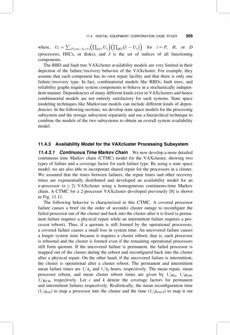
in Fig. 11.11.

The following behavior is characterized in this CTMC. A covered processor

failure causes a brief (in the order of seconds) cluster outage to reconfigure the

failed processor out of the cluster and back into the cluster after it is fixed (a perma-

nent failure requires a physical repair while an intermittent failure requires a pro-

cessor reboot). Thus, if a quorum is still formed by the operational processors,

a covered failure causes a small loss in system time. An uncovered failure causes

a longer system time because it requires a cluster reboot; that is, each processor

is rebooted and the cluster is formed even if the remaining operational processors

still form quorum. If the uncovered failure is permanent, the failed processor is

mapped out of the cluster during the reboot and reconfigured back into the cluster

after a physical repair. On the other hand, if the uncovered failure is intermittent,

the cluster is operational after a cluster reboot. The permanent and intermittent

mean failure times are 1/lp and 1/lI hours, respectively. The mean repair, mean

processor reboot, and mean cluster reboot times are given by 1/mp, 1/mPB,

1/mCB, respectively. Let c and k denote the coverage factors for permanent

and intermittent failures respectively. Realistically, the mean reconfiguration time

(1/mIN) to map a processor into the cluster and the time (1/mOUT) to map it out


of the cluster are different. In the CTMC of Fig. 11.11, we have assumed that mIN ¼

mOUT ¼ mT. The states of the Markov chain are represented by (abc, d ), where,

a ¼ number of processors down with permanent failure

b ¼ number of processors down with intermittent failure

c ¼

0 if both processors are up

p if one processor is being repaired

b if one processor is being rebooted

c if cluster is undergoing a reboot

t if cluster is undergoing a reconfiguration

r if two processors are being rebooted

s if one is being rebooted and other repaired

8>>>>>>>>>>><>>>>>>>>>>>:

d ¼0 cluster up state

1 cluster down state

�

20p,1

10p,0

10c,1 00t,1 10t,1

01c,1

000,0

01t,1

01b,0

02r,1

11s,1

λP

λP

µP

λP

λP

2 2 λP

(1-c)

2 λI(1-k)

µCB

2 λIk

µT

λI

2 µPB

µP

λP

2 λP

λP

µTµ

P

µT µ

PB2 λP

c

µCB

λI

µPB

Figure 11.11 CTMC for the two-processor VAXcluster.


The steady-state availability of the cluster is given by:

Availability ¼ P000,0 þ P10p,0 þ P01b,0 (11:11)

where, Pabc,d denotes the steady-state probability that the process is in state (abc, d ).

We computed the availability of the VAXcluster system by solving the above

CTMC using SHARPE [16], which is a software package for availability/performability analysis. The main problem with this approach was that the size of

the CTMC grew exponentially with the number of processors in the VAXcluster

system. The largeness posed the following challenges: (1) the capability of the

software to solve the model with thousands of states for VAXclusters with n . 5

processors and (2) the problem of actually generating the state space. In the next

section, we address these two drawbacks.

11.4.3.2 Approximate Availability Model for the Processing Sub-system In this section, we discuss a VAXcluster availability model that avoids

the largeness associated with a Markov model. To reduce the complexity of a

large system, Ibe et al. [9] developed a two-level hierarchical model. The bottom

level is a homogeneous CTMC, and the top level is a combinatorial model. This

top-level model was represented as a network of diodes (or three-state devices).

The approximate availability model developed for the analysis made the follow-

ing assumptions [9].

1. The behavior of each processor was modeled by a homogeneous CTMC and

assumed that this processor did not break the quorum rule. This assumption is

justified by the fact that the probability of VAXcluster failure due to loss of

quorum is relatively low.

2. Each processor has an independent repairman. This assumption is justified as

the authors saw that the MTBF was large compared to the MTTR.

These assumptions allowed the authors to decompose the n-processor VAXcluster

into n independent subsystems. Further, the states of the CTMC for the individual

processors were classified into the following three states:

1. X ¼ the set of states in which the processors are up;

2. Y ¼ the set of states in which the cluster is down due to a processor failure; and

3. Z ¼ the set of states in which the processor is down but the cluster is up.

Ibe et al. [9] compared the superstates with the three states of a diode. The three

states X, Y, and Z represent the following states of the diode: up state, the short-

circuit state, and the open-circuit state, respectively. Then the availability, A, of

the VAXcluster was defined as follows [9]:

A ¼ P ½at least one processor in superstate X and none in superstate Y�:


Let nX , nY , and nZ denote the number of processors in superstates X, Y, and Z,

respectively. Let PX , PY , and PZ denote the probability that a processor is in super-

state X, T, and Z. Ibe et al. [9] thus defined the availability An of an n-processor

VAXcluster as follows:

A ¼Xn

nX¼1

n

nX 0 n � nX

� �PnX

X P0Y Pn�nX

Z

¼Xn

nX¼0

n

nX

� �PnX

X Pn�nX

Z �n!

0!(n � 0)!P0

XPnZ ¼ PX þ PZð Þ

n�Pn

Z : (11:12)

Ibe et al. could analyze different VAXcluster configurations by simply varying

the number of processors n in the above equation. The main drawbacks of this

approach are the approximate nature of the solution versus an exact solution, and

the need to make simplifying assumptions, one of the assumptions being an indepen-

dent repairman for each processor. In the next section, we illustrate another approxi-

mation technique to deal with large subsystems.

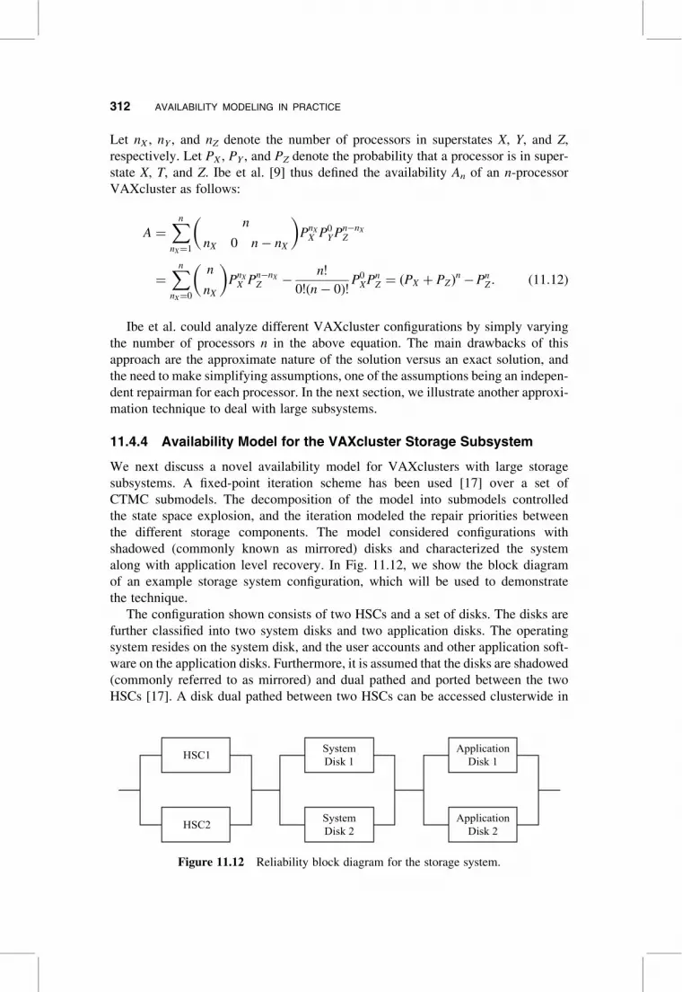
11.4.4 Availability Model for the VAXcluster Storage Subsystem

We next discuss a novel availability model for VAXclusters with large storage

subsystems. A fixed-point iteration scheme has been used [17] over a set of

CTMC submodels. The decomposition of the model into submodels controlled

the state space explosion, and the iteration modeled the repair priorities between

the different storage components. The model considered configurations with

shadowed (commonly known as mirrored) disks and characterized the system

along with application level recovery. In Fig. 11.12, we show the block diagram

of an example storage system configuration, which will be used to demonstrate

the technique.

The configuration shown consists of two HSCs and a set of disks. The disks are

further classified into two system disks and two application disks. The operating

system resides on the system disk, and the user accounts and other application soft-

ware on the application disks. Furthermore, it is assumed that the disks are shadowed

(commonly referred to as mirrored) and dual pathed and ported between the two

HSCs [17]. A disk dual pathed between two HSCs can be accessed clusterwide in

HSC1

HSC2 SystemDisk 2

SystemDisk 1

ApplicationDisk 1

ApplicationDisk 2

Figure 11.12 Reliability block diagram for the storage system.


a coordinated way through either HSC. In case one of the HSC fails, a dual ported

disk can be accessed through the other HSC after a brief failover period.

We now discuss the sequence of approximation models developed to compute the

availability of the storage system in Fig. 11.12. The first model assumed that each

component in the block diagram has its own repair facility. We assumed that the

repair time is a two-stage hypoexponentially distributed random variable with the

first phase being the travel time and the second phase being the actual repair

time. This model can be solved as a pure series-parallel availability model to

compute the availability of the storage system, similar to the solution of the RBD

in Section 11.4.1.

In the second improved model, we removed the assumption of independent

repair. Instead, it is assumed that a repair facility is shared within a subsystem.

The storage system is now assumed as a two-level hierarchical model. The

bottom level consists of three independent CTMC models, namely, HSC, SDisk,

and ADisk, representing the HSC, system disk, and application disk subsystems,

respectively. The top level consists of a reliability block diagram representing a

series network of the three subsystems. In Fig. 11.13(a), (b), (c), we show the

CTMC models of the three subsystems. The reliability block diagram at the top

level is shown in Fig. 11.14.

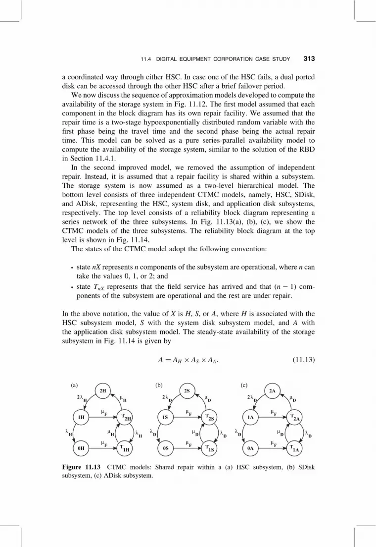
The states of the CTMC model adopt the following convention:

. state nX represents n components of the subsystem are operational, where n can

take the values 0, 1, or 2; and

. state TnX represents that the field service has arrived and that (n 2 1) com-

ponents of the subsystem are operational and the rest are under repair.

In the above notation, the value of X is H, S, or A, where H is associated with the

HSC subsystem model, S with the system disk subsystem model, and A with

the application disk subsystem model. The steady-state availability of the storage

subsystem in Fig. 11.14 is given by

A ¼ AH � AS � AA: (11:13)

2H(a) (b) (c)

1H T2H

0H

H2λ µ

H

Fµ

Fµ

λH H

µ λH

T1H

1S T2S

0S

D2λ µ

D

Fµ

Fµ

λD D

µ λD

T1S

2S 2A

1A T2A

0A

D2λ µ

D

Fµ

Fµ

λD D

µ λD

T1A

Figure 11.13 CTMC models: Shared repair within a (a) HSC subsystem, (b) SDisk

subsystem, (c) ADisk subsystem.


AX is the availability of the X subsystem and is given by

AX ¼ P2X þ P1X þ PT2X(11:14)

where PiX and PTiXare the steady-state probability that the Markov chain is in state

iX and state TiX , respectively.

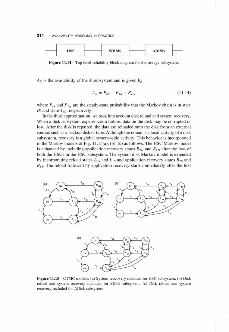
In the third approximation, we took into account disk reload and system recovery.

When a disk subsystem experiences a failure, data on the disk may be corrupted or

lost. After the disk is repaired, the data are reloaded onto the disk from an external

source, such as a backup disk or tape. Although the reload is a local activity of a disk

subsystem, recovery is a global system-wide activity. This behavior is incorporated

in the Markov models of Fig. 11.15(a), (b), (c) as follows. The HSC Markov model

is enhanced by including application recovery states R2H and R1H after the loss of

both the HSCs in the HSC subsystem. The system disk Markov model is extended

by incorporating reload states L2S and L1S and application recovery states R2S and

R1S. The reload followed by application recovery starts immediately after the first

HSC SDISK ADISK

Figure 11.14 Top level reliability block diagram for the storage subsystem.

(a)2H

1H T2H

0H

2 λ µH

Fµ

F

λH λ

H

1H

µ

H

R

µ

µR

µH

λH

µH

2 λH

T

R2H

1HR

(b)

1S T2S

0S

D2 λ µ

D

Fµ

Fµ

λD λ

D

T1S

2Sµ

R

µR

λD

λD

Dµ

µD 2 λ

Dµ

D 2 λD

Sµ

Sµ

R2S

L

L

R

2S

1S1S

(c)

T2A

0A

D2 λ µ

D

Fµ

Fµ

λD λ

D

T1A

µR

µR

λD

λD

Dµ

µD 2 λ

Dµ

D 2 λD

Aµ

Aµ

R2A

L

L

R

2A

1A1A

2A

1A

Figure 11.15 CTMC models: (a) System reocovery included for HSC subsystem, (b) Disk

reload and system recovery included for SDisk subsystem, (c) Disk reload and system

recovery included for ADisk subsystem.


disk is repaired. We further assume that a component could suffer failures during a

reload and/or recovery. The application disk Markov model is extended similar to

the system disk model by including reload states L2A and L1A and recovery states R2A

and R1A. The expression for the steady-state availability of the storage subsystem is

similar to the expression obtained in the second approximation.

In the fourth approximation, the assumption of independent repair facility for

each subsystem is eliminated. In this approximation, the repair facility is shared

between subsystems, and, when more than one component is down, the following

repair priority is assumed: (1) any subsystem with all failed components is repaired

first; otherwise, (2) an HSC is repaired first, system disk second, and application disk

third. This repair priority scheme does not change the Markov model for the HSC

subsystem but changed the model for the system and application disk subsystems.

The system disk has the second highest priority and hence the system disk repair

rate mD is slowed down by multiplying it by P1, the probability that both HSCs

are operational, given that field service is present and the system is not in a recovery

mode. Then P1 is given by

P1 ¼P2H

P2H þ PT1Hþ PT2H

� � : (11:15)

It was previously assumed that a component can be repaired during recovery [17].

The system disk repair rate, mD , from the recovery states is thus slowed down by

multiplying it by P2 where,

P2 ¼PR2H

PR1Hþ PR2H

� � : (11:16)

Here, PRnH(n ¼ 1, 2) are the HSC recovery states.

The application disk has the lowest repair priority and is enforced by probabilis-

tically slowing down the repair rate. The repair rate from the nonrecovery states is

slowed down by multiplying mD by P3 where,

P3 ¼P2H

A�

P2S

B: (11:17)

Here, A ¼ P2H þ PT1Hþ PT2H

and B ¼ P2S þ PT1Sþ PT2S

þ PL1Sþ PL2S

. Then P3

expresses the probability that both HSCs are operational given that the HSC sub-

system is not in the recovery states or in states with less than two HSCs operational

and that both system disks are operational given that the system disk is in nonrecov-

ery states or states with more than one system disk up. The steady-state availability

is computed as in the first approximation.

In the above approximations, we included the field service travel time for each

subsystem. In the real world, if a field service person is present and repairing a com-

ponent in one subsystem, he would respond to a failure in another subsystem. Thus,

in this case, we should not be including travel time twice. Also, the field service

would follow the repair priority described above. The Markov model for each


subsystem can be modified by iteratively checking the presence of field service

person in the other two Markov models. The field service person is assumed to

wait on site until reload and recovery is completed in the SDisk and ADisk

subsystem and until recovery is completed in the HSC subsystem.

The HSC subsystem is extended as follows. The rate of transition due to a

component failure is probabilistically split using the variable y1 (or 1 2 y1). The

probability that the field service is present for repairing a component in either of

the two disk subsystems is

y1 ¼ (1 � P2S � P1S � P0S) þ (1 � P2A � P1A � P0A)

� ((1 � P2S � P1S � P0S) � (1 � P2A � P1A � P0A)): (11:18)

The initial value of y1 is assumed to be 0 in the first iteration, then the above value of

y1 is used for the next iteration.

The system (application) disk subsystem is extended as follows. The rate of every

transition due to a component failure that occurs in the absence of the repair person

in the system (application) disk subsystem is multiplied by y2 (or 1 2 y2). The

expression for y2 is similar to the expression for y1 except S(A) is replaced by H.

This takes into account that the field service is present in the HSC and/or application

(system) disk subsystem.

In a similar manner, the next approximation refined the model by taking into

account the global nature of system recovery. That is, if a recovery is ongoing in

one subsystem, the other two subsystems are forced to go into recovery. The

approximated effect of global recovery is achieved with an iterative scheme that

allows for interaction between the submodels. The final approximation only modi-

fied the HSC subsystem model to incorporate the effect of an HSC failover as shown

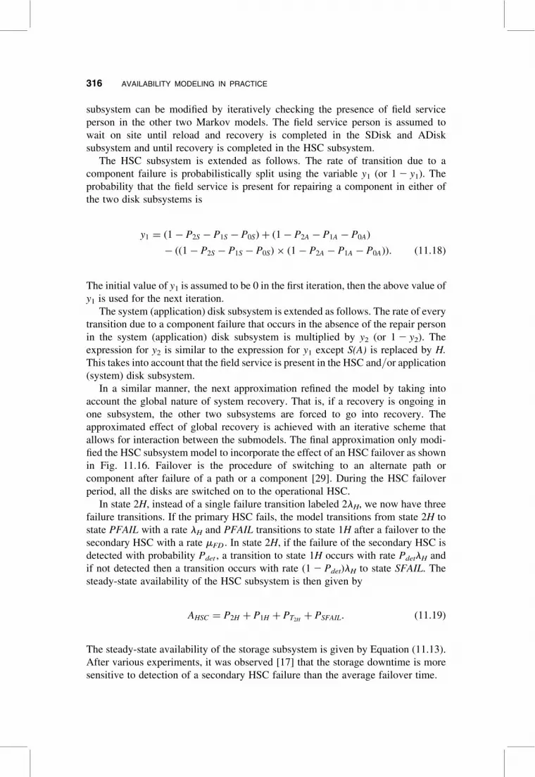
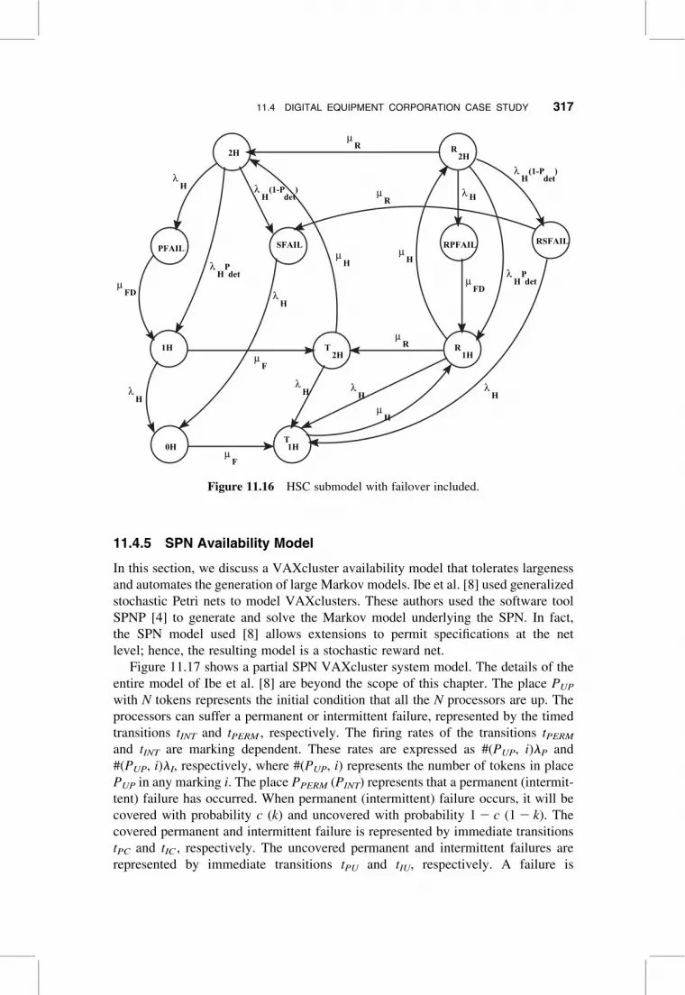
in Fig. 11.16. Failover is the procedure of switching to an alternate path or

component after failure of a path or a component [29]. During the HSC failover

period, all the disks are switched on to the operational HSC.

In state 2H, instead of a single failure transition labeled 2lH, we now have three

failure transitions. If the primary HSC fails, the model transitions from state 2H to

state PFAIL with a rate lH and PFAIL transitions to state 1H after a failover to the

secondary HSC with a rate mFD . In state 2H, if the failure of the secondary HSC is

detected with probability Pdet , a transition to state 1H occurs with rate PdetlH and

if not detected then a transition occurs with rate (1 2 Pdet)lH to state SFAIL. The

steady-state availability of the HSC subsystem is then given by

AHSC ¼ P2H þ P1H þ PT2Hþ PSFAIL: (11:19)

The steady-state availability of the storage subsystem is given by Equation (11.13).

After various experiments, it was observed [17] that the storage downtime is more

sensitive to detection of a secondary HSC failure than the average failover time.


11.4.5 SPN Availability Model

In this section, we discuss a VAXcluster availability model that tolerates largeness

and automates the generation of large Markov models. Ibe et al. [8] used generalized

stochastic Petri nets to model VAXclusters. These authors used the software tool

SPNP [4] to generate and solve the Markov model underlying the SPN. In fact,

the SPN model used [8] allows extensions to permit specifications at the net

level; hence, the resulting model is a stochastic reward net.

Figure 11.17 shows a partial SPN VAXcluster system model. The details of the

entire model of Ibe et al. [8] are beyond the scope of this chapter. The place PUP

with N tokens represents the initial condition that all the N processors are up. The

processors can suffer a permanent or intermittent failure, represented by the timed

transitions tINT and tPERM , respectively. The firing rates of the transitions tPERM

and tINT are marking dependent. These rates are expressed as #(PUP, i)lP and

#(PUP, i)lI, respectively, where #(PUP, i) represents the number of tokens in place

PUP in any marking i. The place PPERM (PINT) represents that a permanent (intermit-

tent) failure has occurred. When permanent (intermittent) failure occurs, it will be

covered with probability c (k) and uncovered with probability 1 2 c (1 2 k). The

covered permanent and intermittent failure is represented by immediate transitions

tPC and tIC , respectively. The uncovered permanent and intermittent failures are

represented by immediate transitions tPU and tIU, respectively. A failure is

2H

1H

0H

PFAIL SFAIL RPFAIL RSFAIL

R2H

R1H

T2H

T1H

λH

FDµ

λH

λH

Pdet

λH

(1-Pdet

)

λH

µH

µF

µF

λH

µH

λH

Hµ

λ H

µFD

λH

Pdet

λH

(1-Pdet

)

Rµ

Rµ

λH

Rµ

Figure 11.16 HSC submodel with failover included.


Blo

ck

Clu

ster

Rec

onfig

urat

ion

P UIF

t IC

P INT

t IU

t IP

λ P#

#λ I

l

Inte

rmitt

ent B

lock

#λ P t PE

RM

P PER

M

1-c

t PC t PU

P P UPF

P RP

REB

P

Perm

anen

t Blo

ck

l INT

REB

t

1-k

CPF

N UP

P

kc

l l

t

µ REC

ON

FIG

REC

ON

FIG

t

Figure

11.17

Par

tial

SP

Nm

od

elo

fth

eV

AX

clu

ster

syst

em.

318

considered to be covered only if the number of operational processors is at least l, the

quorum. The input and output arc with multiplicity l from and to the place PUP

ensures quorum maintenance. In Fig. 11.17, the block labeled, “Cluster Reconfi-

guration Block” represents a group of reconfiguration places in the complete

model [8]. In addition, the following behavior is represented by the SPN.

. A covered permanent failure is not possible while the cluster is being rebooted

after an uncovered failure (token in either PUIF or PUPF). This is represented by

an inhibitor arc from PUIF and PUPF to the immediate transition tPC .

. It is assumed that a failure does not occur while the cluster is being reconfi-

gured. This is represented by the inhibitor arcs from the “Cluster Reconfigura-

tion Block” to tPERM and tINT .

. A processor under reboot can suffer a permanent failure. This is represented by

the fact that when there is a token in PREB both the transitions tREB and tIP are

enabled.

The steady-state availability is given by

A ¼Xi[t

ripi, (11:20)

where t is the set of tangible markings and,

ri ¼

1, if(#(PUP, i) � l )^

½#(P of Cluster Reboot Places, i) , 1 _ #(PUIF , i) , 1�^

½#(P Cluster Reconfiguration Block, i) , 1�

0, otherwise

8>><>>:

11.4.6 SPN Availability Model for Heterogeneous VAXclusters

We now present a SPN model that considers realistic VAXcluster configurations

that include uniprocessors and multiprocessors [18]. The heterogeneity in the

model allowed each multiprocessor to contain varying number of processors, and

each VAX in the VAXcluster to belong to different VAX families. Henceforth,

we refer to the SPN model as the heterogeneous model. Throughout this section

we refer to a single multiprocessor system as a machine, which consists of two

components: one or more processors and a platform. The platform consists of the

memory, power, cooling, console interface module, and I/O channel adapters

[18]. As in the uniprocessor case in the above sections, we depict covered and

uncovered permanent and intermittent failures. In addition, we depict the following

failure/recovery behavior for a multiprocessor. A processor failure in a machine

requires a machine reboot to map the faulty processor offline. The entire machine

is not operational during the processor repair and the reboot following the repair.

Before and after every machine reboot, a cluster reconfiguration maps the machine


out and into the cluster. The platform components of a machine are single points of

failure for that machine [18]. In addition, the following features are included:

. The option of including the quorum disk: a quorum disk acts as a virtual node in

the VAXcluster, casting a “tie-breaker” vote.

. The option of including failure/recovery behavior like unsuccessful repair and

unsuccessful reboots: an unsuccessful repair is modeled by introducing a faulty

repair. Faulty repair means that diagnostics called out a wrong FRU (field

replaceable unit) or that the right FRU was requested but is DOA (dead on

arrival). Unsuccessful reboot means a processor reboot did not complete and

has to be repeated.

. The option of including detailed cluster reconfiguration information: for

example, if the quorum does not exist in reality, the time to form a cluster is

longer than the usual reconfiguration time.

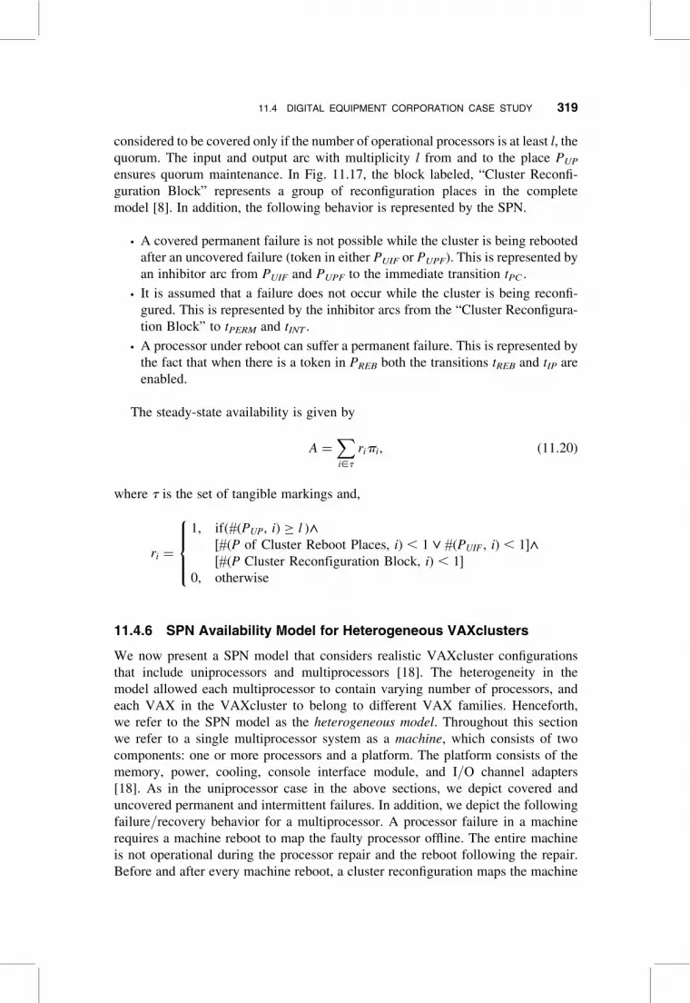
The overall model structure is shown in Fig. 11.18. The VAXcluster is modeled

as a 1 � N array, where each plane represents a subnet of a machine consisting of Mi

processors. The place PUP in plane i contains Mi tokens and represents the initial

condition that the machine is up with Mi processors. The cluster reconfiguration

subnet consists of a single place clust_reconfig, which initially consists of a single

token. Whenever a machine i initiates a reconfiguration, the subnet associated

with it flushes the token out of clust_reconfig and returns the token after the recon-

figuration. This ensures that all machines in the cluster participate in a cluster state

transition. Similarly, the quorum disk is treated as a separate subnet that interacts

with each of the N subnets. The number of processors in a machine is varied by vary-

ing the number of tokens Mi in each subnet. The model allows the machines in the

Figure 11.18 Model structure for the VAXcluster system.


cluster to belong to a different VAX series because every subnet handles the failure/recovery behavior of a machine separately. If Mi ¼ 1 in a subnet, then the machine

follows the failure/recovery behavior of a uniprocessor. The detailed subnet associ-

ated with a machine is beyond the scope of this chapter and has been previously

presented [18].

The heterogeneous SPN model included various extensions like variable arcs,

enabling functions or guards, rate type functions, etc., and hence is a Stochastic

Reward Net [1]. For example, when an intermittent covered failure transition

fires, the rate type function for the rate lIC is defined as

if (Mach UP þ (mark(Pqdup) � NQV) � QU)

lIC ¼ lplatint þ (mark(PUP) � lI)

else

lIC ¼ k � (lplatint þ (mark(PUP) � lI)),

where Mach_UP represents the number of machines up in the cluster, lplatint is the

platform intermittent failure rate, lI is the processor intermittent failure rate, and k

is the probability of a covered intermittent failure. The marking, mark(Pqdup) . 1

implies the quorum disk is up and NQV is the number of quorum votes assigned

to the quorum disk. The number of votes needed for the VAXcluster to be oper-

ational is given by QU. On the other hand, the rate type function for an intermittent

uncovered failure rate is given by, lIU ¼ (1 � k) � (lplatint þ (mark(PUP) � lI)).

The heterogeneous VAXcluster model is available if:

1. mark(clust_reconfig) ¼ 1, that is a cluster reconfiguration is not in progress,

2. NU þ (mark(Pqdup) � NQV ) � QU

where NU is obtained using the following algorithm:

Initial: NU ¼ 0

For i ¼ 1, . . . , N

If ((mark(Platform_failure, i) ¼ 0) AND (mark(PUP , i) . 0) AND

Repair and Reboot Transitions Disabled) then

NU ¼ NU þ 1

NU represents that a machine is up if no platform failure has occurred and that at

least one processor is up and repair or reboot is not in progress.

This heterogeneous model was evaluated using the SPNP package [4]. This pack-

age solved the SPN by analyzing the underlying CTMC. We resolved the problem in

the previous study [18] by using a technique that involved the truncation of the state

space [13]. The state space cardinality of the CTMC isomorphic with the hetero-

geneous model increased with the number of machines in the VAXcluster, as well

as the number of processors in each machine. To implement this state space reduction

technique by specifying a truncation level K for processor failures in the model,

the maximum value of K is M1 þ M2 þ � � � þ MN. The value K specifies that the


reachability graph and hence the corresponding CTMC be generated up to K processor

failures. This is implemented in the model by means of an enabling function associ-

ated with all the failure transitions. The enabling function disables all the failure tran-

sitions ifPN

i¼1 Mi � mark(PUP, i)� �

� K. This technique is justified as follows:

. In real systems, most of the time the system has majority of its components

operational [13]. This means the probability mass is concentrated on a rela-

tively small number of states in comparison to the total number of states in

the model.

. We observed the impact of varying the truncation level on the availability

measures for an example heterogeneous cluster and concluded that the effect

was minimal.

We used the heterogeneous model to not only evaluate measures associated with

standard system availability but also with system reliability and task completion.

In the system reliability class measures, we evaluated measures like frequency of

failures and frequency of disruptive outages. The term disruptive is defined as

follows: any outage that exceeds the specified tolerance limit of the user. The task

completion measures evaluated the probability that the application is interrupted

during its application period.

In this chapter, we discuss an example measure from each of the three classes of

measures [18]:

. Mean Cluster Downtime D in minutes per year: This is a system availability

measure and represents the average amount of time the cluster is not operating

during a one year observation period. Then the expression for D in terms of the

steady state cluster availability, A is given by, D ¼ (1 2 A) � 8760 � 60.

. Frequency of Disruptive Reconfigurations (FDR): This is a system reliability

measure and represents the mean number of reconfigurations which exceed

the specified tolerance duration during the one year observation period.

We evaluate FDR as, FDR ¼ mrg � ethresh�mrg � Prg � 8760 � 60, where mrg

is the cluster reconfiguration (in, out, or formation) rate, thresh is the time

units of the specified tolerance duration on the reconfiguration times, and Prg

is the probability that a reconfiguration is in progress.

. Probability of Task Interruption under Pessimistic Assumption(Prob_Psm): This is a task completion measure. It measures the probability

of a task that initially finds the system available and that needs x hours for

execution, but is interrupted by any failure in the cluster. This is a pessimistic

assumption because the system does not tolerate any interruption including the

brief reconfiguration delays. The expression for Prob_Psm is given by:

Prob Psm ¼

Pj[Upstate 1:0 � e�

PN

k¼1ck,j lp,kþli,kð Þþ lplt,kþlplt int,kð Þð Þx

� �A

Pj,


where for machine k, ck,j is the number of operational processors, Pj is the prob-

ability of being in an operational state, lp,k (li,k) is the processor permanent

(intermittent) failure rate, lplt,k (lplt_int,k) is the platform permanent (intermit-

tent) failure rates for machine k, and A is the cluster availability.

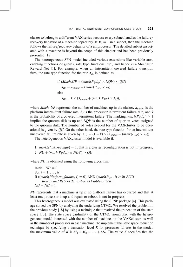
Previously [18], we used these three measures for a particular configuration to

study the impact of truncation. In Table 11.4, we present the number of states

and, the number of transitions of the underlying CTMC. On observing the results,

we can conclude that we could truncate the state space of the SPN model for the

heterogeneous cluster without impacting the results.

11.5 CONCLUSION

We started by briefly discussing various non-state space and state space availability

and performance modeling approaches. Using the problem of deciding the optimal

number of processors in an n-component parallel multiprocessor system, we showed

the limitations of a pure availability or pure performance model and emphasized the

need for a composite availability and performance model. Finally, we took a case

study from a corporate environment and demonstrated an application of the tech-

niques in a real situation. Several approximations and assumptions were made

and validated before use, in order to deal with the size and complexity of the

models encountered.

REFERENCES

1. D. R. Avresky. Hardware and Software Fault Tolerance in Parallel Computing Systems.

Ellis Horwood Ltd., New York, 1992.

2. E. Balkovich, P. Bhabhalia, W. Dunnington, and T. Weyant. ‘VAXcluster availability

modeling.’ Digital Technical Journal, no. 5, pp. 69–79, September 1987.

3. G. Bolch, S. Greiner, H. de Meer, and K. S. Trivedi. Queueing Networks and Markov

Chains—Modeling and Performance Evaluation with Computer Science Applications.

John Wiley & Sons, 1998.

TABLE 11.4 Effect of State Truncation on Output Measures.

Trunc.

Level

No. of

States

No. of

Arcs

Mean Cluster

Downtime,

min/yr

Freq. of

Disruptive, reconfig.

threshold ¼ 10 s

Prob. of Task

Interruption,

t ¼ 1,000 s

1 348 948 12.91732078 9.96432050 0.00032767

2 2,088 7,110 13.00257283 9.96751584 0.00032767

3 6,394 26,686 13.00258549 9.96751604 0.00032767

4 13,236 66,596 13.00258549 9.96751604 0.00032767

5 20,728 122,746 13.00258549 9.96751604 0.00032767

REFERENCES 323

4. G. Ciardo, J. Muppala, and K. S. Trivedi. SPNP: stochastic Petri net package. Proc. Third

Int. Workshop on Petri Nets and Performance Models (PNPM89), Kyoto, Japan,

pp. 142–151, 1989.

5. S. A. Doyle and J. B. Dugan. Dependability assessment using binary decision diagrams.

Proc. 25th Intl. Symposium on Fault Tolerant Computing, pp. 249–258, 1995.

6. S. A. Doyle, J. B. Dugan, and M. Boyd. Combinatorial models and coverage: a binary

decision diagram (BDD) approach. Proc. Annual Reliability and Maintainability

Symposium, pp. 82–89, 1995.

7. K. Goseva-Popstojanova and K. S. Trivedi. Stochastic modeling formalisms for depend-

ability, performance and performability. Performance Evaluation—Origins and Direc-

tions, Lecture Notes in Computer Science (edited by G. Haring, C. Lindemann, and

M. Reiser). Springer Verlag, pp. 385–404, 2000.

8. O. Ibe, A. Sathaye, R. Howe, and K. S. Trivedi. Stochastic Petri net modeling of

VAXcluster system availability. Proc. Third International Workshop on Petri Nets and

Performance Models (PNPM89), Kyoto, Japan, pp. 112–121, 1989.

9. O. C. Ibe, R. C. Howe, and K. S. Trivedi. Approximate availability analysis of

VAXcluster systems. IEEE Transactions on Reliability, vol. 38, no. 1, pp. 146–152,

April 1989.

10. N. P. Kronenberg, H. M. Levy, W. D. Strecker, and R. J. Merwood. VAXclusters: a

closely coupled distributed system. ACM Trans. Computer Systems, vol. 4, pp. 130–146,

May 1986.

11. T. Luo and K. S. Trivedi. ‘An improved algorithm for coherent-system reliability.’ IEEE

Transactions on Reliability, vol. 47, no. 1, pp. 73–78, 1998.

12. J. F. Meyer. On evaluating the performability of degradable computer systems. IEEE

Transactions on Computers, vol. 29, no. 8, pp. 720–731, 1980.

13. R. Muntz, E. de Souza e Silva, and A. Goyal. Bounding availability of repairable com-

puter systems. IEEE Trans. on Computers, vol. 38, no. 12, pp. 1714–1723, December

1989.

14. J. Muppala, A. Sathaye, R. Howe, and K. S. Trivedi. Dependability modeling of a hetero-

geneous VAXcluster system using stochastic reward nets. Hardware and Software Fault

Tolerance in Parallel Computing Systems (edited by D. Avresky). Ellis Horwood Ltd.,

pp. 33–59, 1992.

15. J. Muppala and K. S. Trivedi. Numerical transient solution of finite markovian queueing

systems. Queueing and Related Models (edited by U. N. Bhat and I. V. Basawa). Oxford

University Press, pp. 262–284, 1992.

16. R. Sahner, A. Puliafito, and K. S. Trivedi. Performance and Reliability Analysis of Com-

puter Systems: An Example-Based Approach Using the SHARPE Software Package.

Boston: Kluwer Academic Publishers, 1995.

17. A. Sathaye, K. S. Trivedi, and D. Heimann. Approximate Availability Models of the

Storage Subsystem. Technical Report, DEC., September 1988.

18. A. Sathaye, K. S. Trivedi, and R. Howe. Availability modeling of heterogeneous

VAXcluster systems: a stochastic Petri net approach. Proc. of International Conference

on Fault-Tolerant Systems, Varna, January 1990.

19. A. Satyanarayana and A. Prabhakar. New topological formula and rapid algorithm for

reliability analysis of complex networks. IEEE Transactions on Reliability, vol. 27, pp.

82–100, 1978.


20. D. Siewiorek and R. Swarz. The Theory and Practice of Reliable System Design. Digital

Press, 1982.

21. R. M. Smith, K. S. Trivedi, and A. V. Ramesh. Performability analysis: measures, an

algorithm, and a case study. IEEE Transactions on Computers, vol. 37, no. 4, pp.

406–417, April 1988.

22. H. Sun, X. Zang, and K. S. Trivedi. A BDD-based algorithm for reliability analysis of

phased-mission systems. IEEE Transactions on Reliability, vol. 48, no. 1, pp. 50–60,

March 1999.

23. L. Tomek and K. S. Trivedi. Fixed point iteration in availability modeling. In Informatik-

Fachberichte, Fehlertolerierende Rechensysteme (edited by M. Dal Cin). Berlin:

Springer-Verlag, vol. 283, pp. 229–240, 1991.

24. K. S. Trivedi, A. Sathaye, O. Ibe, and R. Howe. Should I add a processor? Proc. 23rd

Annual Hawaii Conference on System Sciences, pp. 214–221, January 1990.

25. K. S. Trivedi. Probability and Statistics with Reliability, Queuing and Computer Science

Applications (2nd ed.). New York: John Wiley & Sons, 2001.

26. B. Tuffin and K. S. Trivedi. Implementation of importance splitting techniques in stochas-

tic Petri net package. Computer Performance Evaluation: Modelling Tools and Tech-

niques; 11th International Conference; TOOLS 2000, Schaumburg, IL, (edited by

B. Haverkort, H. Bohnenkamp, and C. Smith). Lecture Notes in Computer Science

1786. Springer Verlag, 2000.

27. B. Tuffin and K. S. Trivedi. Importance sampling for the simulation of stochastic

Petri nets and fluid stochastic Petri nets. Proceedings of High Performance Computing,

Seattle, WA, April 2001.

28. X. Zang, D. Wang, H. Sun, and K. S. Trivedi. A BDD-based algorithm for analysis

of multistate components. IEEE Transactions on Computers, vol. 52, no. 12,

pp. 1608–1618, December 2003.

29. Introduction to VAXcluster Application Design. Digital Equipment Corporation, 1984.

REFERENCES 325

availability models in practice

Documents