service availability and discovery responsiveness
TRANSCRIPT

Service Availability and
Discovery Responsiveness
A User-Perceived View on Service Dependability
Dissertation
zur Erlangung des akademischen GradesDr. rer. nat. im Fach Informatik
eingereicht an der Mathematisch-Naturwissenschaftlichen Fakultatder Humboldt-Universitat zu Berlin am 9. Dezember 2014
von Herrn Dipl.-Inf. Andreas Dittrich
Prasident der Humboldt-Universitat zu BerlinProf. Dr. Jan-Hendrik Olbertz
Dekan der Mathematisch-Naturwissenschaftlichen FakultatProf. Dr. Elmar Kulke
Gutachter:
1. Prof. Dr. Miroslaw Malek2. Prof. Dr. Alexander Reinefeld3. Prof. Dr. Jorg Kaiser
Tag der mundlichen Prufung: 20. Marz 2015


To Tante Maria.


Preface
Almost 2400 years ago Plato wrote the allegory of the cave, in which Plato’s brotherGlaucon and his mentor Socrates discuss the difference between the form and thesensation. Socrates describes a group of people who have lived their entire liveinside a cave. The only knowledge about the outside world comes from shadowsprojected to the walls of the cave of people and objects passing by outside. Theseshadows are mere sensations of the true form outside the cave. Nonetheless, for thepeople inside the cave there is but this one perception which constitutes their reality.
In computer networks, every node has its own view on the network and the ser-vices therein, which is defined by the network components that allow the node tocommunicate with the rest of the network. While a global perspective on the net-work, the awareness of the form in Plato’s words, is generally desirable it mightbe of limited value to a node with only its own perspective. When improving thequality of service provision it is thus important to keep the node-specific perspec-tive in mind. Improving as many as possible node-specific perspectives will in turnimprove the overall quality of service provision. This work focuses on the evalua-tion of node or user-perceived views on service quality as reflected in two differentdependability properties, availability and responsiveness.
Berlin, March 2015 Andreas Dittrich
vii


Acknowledgements
First and foremost, I would like to thank my doctoral advisor Miroslaw Malek forhis continuous support and inspiration. He made me look further so often when Ithought I had seen it all. I would also like to thank Felix Salfner for all the technicaladvice he was able to give me and for making me believe that I can actually finishthis work. I am very grateful to Katinka Wolter for encouraging me during the lastyear and for demonstrating me again and again the beauty of math. This work was inparts carried out in the graduate school METRIK and I am thankful to have been ableto present my work in front of experts from so many different fields. This helped meto strengthen and to focus. I am especially grateful to Joachim Fischer who alwayshad an open ear from the moment I started this work. Of course I cannot name allmy fellow colleagues I would like to thank for the many fruitful discussions duringthe work on this thesis.
Last but not least, I want to thank my family, my parents, my brothers and sisterfor always being there when I needed strength and for having the patience when Icould not be there. Ce l’ho fatta Manu! Words cannot tell how much your supportmeans to me. I am most grateful to Tante Maria, who made me believe that there issunshine in every moment of our lives. She gave me the inspiration to start and thecourage to continue.
ix


Abstract
Services play an increasingly important role in modern networks, ranging from webservice provision of global businesses to the Internet of Things. Dependability ofservice provision is thus one of the primary goals. For successful provision, a ser-vice first needs to be discovered and connected to by a client. Then, during actualservice usage, it needs to perform according to the requirements of the client. Sinceproviders and clients are part of a connecting Information and CommunicationsTechnology (ICT) infrastructure, service dependability varies with the position ofactors as the ICT devices needed for service provision change. Service dependabil-ity models need to incorporate these user-perceived perspectives.
We present two approaches to quantify user-perceived service dependability. Thefirst is a model-driven approach to calculate instantaneous service availability. Us-ing input models of the service, the infrastructure and a mapping between the twoto describe actors of service communication, availability models are automaticallycreated by a series of model to model transformations. The feasibility of the ap-proach is demonstrated using exemplary services in the network of University ofLugano, Switzerland. The second approach aims at the responsiveness of the ser-vice discovery layer, the probability to find service instances within a deadline evenin the presence of faults, and is the main part of this thesis. We present a hierarchyof stochastic models to calculate user-perceived responsiveness based on monitor-ing data from the routing layer. Extensive series of experiments have been run on theDistributed Embedded Systems (DES) wireless testbed at Freie Universitat Berlin.They serve both to demonstrate the shortcomings of current discovery protocols inmodern dynamic networks and to validate the presented stochastic models.
Both approaches demonstrate that the dependability of service provision indeeddiffers considerably depending on the position of service clients and providers, evenin highly reliable wired networks. The two approaches enable optimization of ser-vice networks with respect to known or predicted usage patterns. Furthermore, theyanticipate novel service dependability models which combine service discovery,timeliness, placement and usage, areas that until now have been treated to a largeextent separately.
xi


Zusammenfassung
Die Bedeutung von Diensten in modernen Netzwerken nimmt stetig zu. Verlass-liche Dienstbereitstellung ist daher eines der wichtigsten Ziele. Um erfolgreicheinen Dienst erbringen zu konnen, muss dieser zuerst von einem Nutzer gefun-den und verbunden werden. Wahrend der Nutzung muss der Dienst eine Leis-tung entsprechend der Anforderungen des Nutzers erbringen. Da Anbieter undNutzer Teil einer Informations und Kommunikationstechnologie (IKT) Infrastruk-tur sind, wird die Verlasslichkeit der Dienste je nach Position der Aktoren variieren,so wie sich die fur die Bereitstellung notigen IKT Gerate andern. Dienstverlass-lichkeitsmodelle sollten diese nutzerspezifischen Perspektiven berucksichtigen.
Wir stellen zwei Ansatze zur Quantifizierung nutzerspezifischer Dienstverlass-lichkeit vor. Der erste, modellgetriebene Ansatz berechnet momentane Dienstver-fugbarkeit. Aus Modellen des Dienstes, der Infrastruktur und einer Abbildung zwi-schen den beiden, welche die Aktoren der Dienstkommunikation beschreibt, wer-den durch eine Serie von Modelltransformationen automatisiert Verfugbarkeitsmo-delle generiert. Die Realisierbarkeit des Ansatzes wird beispielhaft gezeigt anhandvon Diensten im Netzwerk der Universitat Lugano, Schweiz. Der zweite Ansatz be-handelt die Responsivitat der Dienstfindung, die Wahrscheinlichkeit innerhalb einerFrist Dienstinstanzen zu finden, unter der Annahme von Fehlern. Dies stellt denHauptteil dieser Arbeit dar. Eine Hierarchie stochastischer Modelle wird vorgestellt,die nutzerspezifische Responsivitat auf Basis von Messdaten der Routingebeneberechnet. Umfangreiche Experimente wurden im Distributed Embedded Systems(DES) Funktestbett der Freien Universitat Berlin durchgefurt. Diese zeigen dieProbleme aktueller Dienstfindungsprotokolle in modernen, dynamischen Netzwer-ken. Gleichzeitig dienen sie der Validierung der vorgestellten Modelle.
Beide Ansatze zeigen, daß die Verlasslichkeit der Dienstbereitstellung in der Tatdeutlich mit der Position von Nutzern und Anbietern variiert, sogar in hochverfug-baren Kabelnetzwerken. Die Ansatze ermoglichen die Optimierung von Dienst-netzwerken anhand bekannter oder erwarteter Nutzungsmuster. Zudem antizipierensie neuartige Verlasslichkeitsmodelle, welche Dienstfindung, zeitige Bereitstellung,Platzierung und Nutzung kombinieren; Gebiete, die bisher im Allgemeinen getrenntbehandelt wurden.
xiii


Contents
Preface . . . . . . . . . . . . . . . . . . . . . . . . . . . . . . . . . . . . . . . . . . . . . . . . . . . . . . . . . . . . vii
Acknowledgements . . . . . . . . . . . . . . . . . . . . . . . . . . . . . . . . . . . . . . . . . . . . . . . . . ix
Abstract . . . . . . . . . . . . . . . . . . . . . . . . . . . . . . . . . . . . . . . . . . . . . . . . . . . . . . . . . . . xi
Contents . . . . . . . . . . . . . . . . . . . . . . . . . . . . . . . . . . . . . . . . . . . . . . . . . . . . . . . . . . xv
Acronyms . . . . . . . . . . . . . . . . . . . . . . . . . . . . . . . . . . . . . . . . . . . . . . . . . . . . . . . . . xxi
Part I Introduction
1 Introduction, Motivation, Problem Statement and Main Contributions 31.1 Introduction . . . . . . . . . . . . . . . . . . . . . . . . . . . . . . . . . . . . . . . . . . . . . . . 31.2 Problem Statement . . . . . . . . . . . . . . . . . . . . . . . . . . . . . . . . . . . . . . . . . 6
1.2.1 User-Perceived Service Availability . . . . . . . . . . . . . . . . . . . . . 71.2.2 User-Perceived Service Discovery Responsiveness . . . . . . . . 8
1.3 Approach . . . . . . . . . . . . . . . . . . . . . . . . . . . . . . . . . . . . . . . . . . . . . . . . . 91.4 Main Contributions . . . . . . . . . . . . . . . . . . . . . . . . . . . . . . . . . . . . . . . . . 101.5 Structure of the Manuscript . . . . . . . . . . . . . . . . . . . . . . . . . . . . . . . . . . 11
2 Background and Related Work . . . . . . . . . . . . . . . . . . . . . . . . . . . . . . . . . . 132.1 Service-Oriented Computing . . . . . . . . . . . . . . . . . . . . . . . . . . . . . . . . . 13
2.1.1 Zero Configuration Networking . . . . . . . . . . . . . . . . . . . . . . . . 142.1.2 Service Composition . . . . . . . . . . . . . . . . . . . . . . . . . . . . . . . . . 15
2.2 Service Discovery . . . . . . . . . . . . . . . . . . . . . . . . . . . . . . . . . . . . . . . . . . 162.2.1 Service Discovery Architectures . . . . . . . . . . . . . . . . . . . . . . . . 182.2.2 Service Discovery Protocols . . . . . . . . . . . . . . . . . . . . . . . . . . . 19
2.3 Service Dependability . . . . . . . . . . . . . . . . . . . . . . . . . . . . . . . . . . . . . . . 232.3.1 Availability . . . . . . . . . . . . . . . . . . . . . . . . . . . . . . . . . . . . . . . . . 242.3.2 Availability Evaluation . . . . . . . . . . . . . . . . . . . . . . . . . . . . . . . 26
xv

xvi Contents
2.3.3 Responsiveness . . . . . . . . . . . . . . . . . . . . . . . . . . . . . . . . . . . . . . 292.3.4 Performability, Resilience and Survivability . . . . . . . . . . . . . . 302.3.5 Service Discovery Dependability . . . . . . . . . . . . . . . . . . . . . . . 30
2.4 Modeling Service Networks . . . . . . . . . . . . . . . . . . . . . . . . . . . . . . . . . . 332.5 Wireless Communication . . . . . . . . . . . . . . . . . . . . . . . . . . . . . . . . . . . . 35
2.5.1 Packet Transmission Times . . . . . . . . . . . . . . . . . . . . . . . . . . . . 362.5.2 Network-Wide Broadcasts . . . . . . . . . . . . . . . . . . . . . . . . . . . . . 372.5.3 Wireless Service Discovery . . . . . . . . . . . . . . . . . . . . . . . . . . . . 38
2.6 Conclusion . . . . . . . . . . . . . . . . . . . . . . . . . . . . . . . . . . . . . . . . . . . . . . . . 39
3 ExCovery – A Framework for Distributed System Experiments . . . . . . 413.1 Introduction . . . . . . . . . . . . . . . . . . . . . . . . . . . . . . . . . . . . . . . . . . . . . . . 413.2 The Art of Experimentation . . . . . . . . . . . . . . . . . . . . . . . . . . . . . . . . . . 42
3.2.1 Experiments in Computer Science . . . . . . . . . . . . . . . . . . . . . . 433.2.2 Experiment Factors . . . . . . . . . . . . . . . . . . . . . . . . . . . . . . . . . . 433.2.3 Experiment Design . . . . . . . . . . . . . . . . . . . . . . . . . . . . . . . . . . . 443.2.4 Experiment Validity . . . . . . . . . . . . . . . . . . . . . . . . . . . . . . . . . . 443.2.5 Experimentation Environment . . . . . . . . . . . . . . . . . . . . . . . . . 45
3.3 The Experimentation Environment ExCovery . . . . . . . . . . . . . . . . . . . 473.4 Measurement and Storage Concept . . . . . . . . . . . . . . . . . . . . . . . . . . . . 49
3.4.1 Measurement Data . . . . . . . . . . . . . . . . . . . . . . . . . . . . . . . . . . . 493.4.2 Storage and Conditioning . . . . . . . . . . . . . . . . . . . . . . . . . . . . . 50
3.5 Abstract Experiment Description . . . . . . . . . . . . . . . . . . . . . . . . . . . . . . 523.5.1 Platform Definition . . . . . . . . . . . . . . . . . . . . . . . . . . . . . . . . . . . 553.5.2 Experiment Execution from Factor Definition . . . . . . . . . . . . 55
3.6 Process Description . . . . . . . . . . . . . . . . . . . . . . . . . . . . . . . . . . . . . . . . . 563.6.1 Manipulation Processes . . . . . . . . . . . . . . . . . . . . . . . . . . . . . . . 583.6.2 Manipulation Process Description . . . . . . . . . . . . . . . . . . . . . . 593.6.3 Experiment Process Description . . . . . . . . . . . . . . . . . . . . . . . . 60
3.7 Prototype Implementation . . . . . . . . . . . . . . . . . . . . . . . . . . . . . . . . . . . 633.8 Conclusion . . . . . . . . . . . . . . . . . . . . . . . . . . . . . . . . . . . . . . . . . . . . . . . . 65
Part II User-Perceived Service Availability
4 Modeling User-Perceived Service Dependability . . . . . . . . . . . . . . . . . . . 694.1 Introduction . . . . . . . . . . . . . . . . . . . . . . . . . . . . . . . . . . . . . . . . . . . . . . . 694.2 Model Specification . . . . . . . . . . . . . . . . . . . . . . . . . . . . . . . . . . . . . . . . 70
4.2.1 ICT Infrastructure Model . . . . . . . . . . . . . . . . . . . . . . . . . . . . . . 714.2.2 Service Model . . . . . . . . . . . . . . . . . . . . . . . . . . . . . . . . . . . . . . . 734.2.3 Network Mapping Model . . . . . . . . . . . . . . . . . . . . . . . . . . . . . 744.2.4 Input Model Considerations . . . . . . . . . . . . . . . . . . . . . . . . . . . 76
4.3 Methodology . . . . . . . . . . . . . . . . . . . . . . . . . . . . . . . . . . . . . . . . . . . . . . 764.3.1 Path Discovery Algorithm . . . . . . . . . . . . . . . . . . . . . . . . . . . . . 804.3.2 User-perceived Service Infrastructure . . . . . . . . . . . . . . . . . . . 81
4.4 User-perceived Availability Model Generation . . . . . . . . . . . . . . . . . . 81

Contents xvii
4.4.1 Instantaneous Availability Evaluation . . . . . . . . . . . . . . . . . . . 834.4.2 Access Time Definition . . . . . . . . . . . . . . . . . . . . . . . . . . . . . . . 86
5 Case Study of User-Perceived Service Availability . . . . . . . . . . . . . . . . . . 895.1 Introduction . . . . . . . . . . . . . . . . . . . . . . . . . . . . . . . . . . . . . . . . . . . . . . . 895.2 User-Perceived Service Infrastructure . . . . . . . . . . . . . . . . . . . . . . . . . . 90
5.2.1 Identification and Modeling of ICT Components . . . . . . . . . . 905.2.2 ICT Infrastructure Modeling . . . . . . . . . . . . . . . . . . . . . . . . . . . 915.2.3 Identifcation and Modeling of Services . . . . . . . . . . . . . . . . . . 935.2.4 Service Mapping Pair Generation . . . . . . . . . . . . . . . . . . . . . . . 945.2.5 Model Space Import . . . . . . . . . . . . . . . . . . . . . . . . . . . . . . . . . . 955.2.6 Path Discovery for Service Mapping Pairs . . . . . . . . . . . . . . . 955.2.7 User-Perceived Infrastructure Model Generation . . . . . . . . . . 96
5.3 User-Perceived Steady-State Availability . . . . . . . . . . . . . . . . . . . . . . . 965.4 User-Perceived Instantaneous Availability . . . . . . . . . . . . . . . . . . . . . . 100
5.4.1 Different User Perspectives . . . . . . . . . . . . . . . . . . . . . . . . . . . . 1005.4.2 Adding and Replacing Equipment . . . . . . . . . . . . . . . . . . . . . . 103
5.5 Conclusion . . . . . . . . . . . . . . . . . . . . . . . . . . . . . . . . . . . . . . . . . . . . . . . . 105
Part III Service Discovery Responsiveness
6 Experimental Evaluation of Discovery Responsiveness . . . . . . . . . . . . . 1096.1 Introduction . . . . . . . . . . . . . . . . . . . . . . . . . . . . . . . . . . . . . . . . . . . . . . . 1096.2 Service Discovery Scenarios . . . . . . . . . . . . . . . . . . . . . . . . . . . . . . . . . 111
6.2.1 Scenario I – Single Service Discovery . . . . . . . . . . . . . . . . . . . 1116.2.2 Scenario II – Timely Service Discovery . . . . . . . . . . . . . . . . . 1126.2.3 Scenario III – Multiple Service Discovery . . . . . . . . . . . . . . . . 112
6.3 Experiment Setup . . . . . . . . . . . . . . . . . . . . . . . . . . . . . . . . . . . . . . . . . . 1136.3.1 Virtual Testbed . . . . . . . . . . . . . . . . . . . . . . . . . . . . . . . . . . . . . . 1146.3.2 Wireless Testbed . . . . . . . . . . . . . . . . . . . . . . . . . . . . . . . . . . . . . 116
6.4 Experiment Results . . . . . . . . . . . . . . . . . . . . . . . . . . . . . . . . . . . . . . . . . 1206.4.1 Scenario Results – Single Service Discovery . . . . . . . . . . . . . 1206.4.2 Scenario Results – Timely Service Discovery . . . . . . . . . . . . . 1236.4.3 Scenario Results – Multiple Service Discovery . . . . . . . . . . . 126
6.5 Experiment Results of Testbed Behavior . . . . . . . . . . . . . . . . . . . . . . . 1296.5.1 Response Times over All Runs . . . . . . . . . . . . . . . . . . . . . . . . . 1306.5.2 Topology Changes over Time . . . . . . . . . . . . . . . . . . . . . . . . . . 1326.5.3 Node Clock Drift over Time . . . . . . . . . . . . . . . . . . . . . . . . . . . 134
6.6 Conclusion . . . . . . . . . . . . . . . . . . . . . . . . . . . . . . . . . . . . . . . . . . . . . . . . 135
7 Modeling Service Discovery Responsiveness . . . . . . . . . . . . . . . . . . . . . . . 1377.1 Introduction . . . . . . . . . . . . . . . . . . . . . . . . . . . . . . . . . . . . . . . . . . . . . . . 1377.2 A Model for Service Discovery . . . . . . . . . . . . . . . . . . . . . . . . . . . . . . . 138
7.2.1 Service Discovery Model . . . . . . . . . . . . . . . . . . . . . . . . . . . . . 1397.2.2 Retry Operation Model . . . . . . . . . . . . . . . . . . . . . . . . . . . . . . . 1417.2.3 Network Mapping Model . . . . . . . . . . . . . . . . . . . . . . . . . . . . . 142

xviii Contents
7.2.4 Transmission Time Distributions . . . . . . . . . . . . . . . . . . . . . . . 1437.3 Multicast Reachability Estimation . . . . . . . . . . . . . . . . . . . . . . . . . . . . . 144
7.3.1 Network Model . . . . . . . . . . . . . . . . . . . . . . . . . . . . . . . . . . . . . . 1447.3.2 Reachability Metrics for Network-wide Broadcasts . . . . . . . . 1457.3.3 Calculation of Reachability . . . . . . . . . . . . . . . . . . . . . . . . . . . . 1457.3.4 Probabilistic Breadth-First Search . . . . . . . . . . . . . . . . . . . . . . 146
7.4 Multicast Reachability Validation . . . . . . . . . . . . . . . . . . . . . . . . . . . . . 1487.4.1 Theoretical Validation . . . . . . . . . . . . . . . . . . . . . . . . . . . . . . . . 1487.4.2 Experimental Validation . . . . . . . . . . . . . . . . . . . . . . . . . . . . . . 1507.4.3 Discussion Validation . . . . . . . . . . . . . . . . . . . . . . . . . . . . . . . . . 153
7.5 Model Generation and Solution . . . . . . . . . . . . . . . . . . . . . . . . . . . . . . . 1547.6 Case Study . . . . . . . . . . . . . . . . . . . . . . . . . . . . . . . . . . . . . . . . . . . . . . . . 155
7.6.1 Scenario 1 – Single Pair Responsiveness . . . . . . . . . . . . . . . . . 1557.6.2 Scenario 2 – Average Provider Responsiveness . . . . . . . . . . . 1567.6.3 Scenario 3 – Expected Responsiveness Distance . . . . . . . . . . 157
7.7 Conclusion . . . . . . . . . . . . . . . . . . . . . . . . . . . . . . . . . . . . . . . . . . . . . . . . 159
8 Correlating Model and Measurements . . . . . . . . . . . . . . . . . . . . . . . . . . . . 1618.1 Introduction . . . . . . . . . . . . . . . . . . . . . . . . . . . . . . . . . . . . . . . . . . . . . . . 1618.2 Experiment Setup . . . . . . . . . . . . . . . . . . . . . . . . . . . . . . . . . . . . . . . . . . 162
8.2.1 Varying Data Rate Scenario . . . . . . . . . . . . . . . . . . . . . . . . . . . 1648.2.2 Varying Radio Power . . . . . . . . . . . . . . . . . . . . . . . . . . . . . . . . . 1658.2.3 Input Data Preparation . . . . . . . . . . . . . . . . . . . . . . . . . . . . . . . . 165
8.3 Correlation of Model and Experiments . . . . . . . . . . . . . . . . . . . . . . . . . 1668.4 Experiments with Variable Load . . . . . . . . . . . . . . . . . . . . . . . . . . . . . . 168
8.4.1 Full Model Hierarchy . . . . . . . . . . . . . . . . . . . . . . . . . . . . . . . . . 1698.4.2 Discovery Model . . . . . . . . . . . . . . . . . . . . . . . . . . . . . . . . . . . . 170
8.5 Experiments with Variable Radio Power . . . . . . . . . . . . . . . . . . . . . . . 1718.5.1 Full Model Hierarchy . . . . . . . . . . . . . . . . . . . . . . . . . . . . . . . . . 1728.5.2 Discovery Model . . . . . . . . . . . . . . . . . . . . . . . . . . . . . . . . . . . . 1738.5.3 One Hop Experiments . . . . . . . . . . . . . . . . . . . . . . . . . . . . . . . . 174
8.6 Conclusion . . . . . . . . . . . . . . . . . . . . . . . . . . . . . . . . . . . . . . . . . . . . . . . . 175
Part IV Conclusions
9 Conclusions and Outlook . . . . . . . . . . . . . . . . . . . . . . . . . . . . . . . . . . . . . . . 1799.1 User-Perceived Dependability . . . . . . . . . . . . . . . . . . . . . . . . . . . . . . . . 1799.2 Service Availability Evaluation . . . . . . . . . . . . . . . . . . . . . . . . . . . . . . . 180
9.2.1 Output Models . . . . . . . . . . . . . . . . . . . . . . . . . . . . . . . . . . . . . . 1819.2.2 Case Study . . . . . . . . . . . . . . . . . . . . . . . . . . . . . . . . . . . . . . . . . 1819.2.3 Outlook . . . . . . . . . . . . . . . . . . . . . . . . . . . . . . . . . . . . . . . . . . . . 182
9.3 Evaluation of Service Discovery Responsiveness . . . . . . . . . . . . . . . . 1829.3.1 Experimental Evaluation . . . . . . . . . . . . . . . . . . . . . . . . . . . . . . 1839.3.2 Stochastic Modeling . . . . . . . . . . . . . . . . . . . . . . . . . . . . . . . . . . 1849.3.3 Outlook . . . . . . . . . . . . . . . . . . . . . . . . . . . . . . . . . . . . . . . . . . . . 186

Contents xix
References to Works of the Author . . . . . . . . . . . . . . . . . . . . . . . . . . . . . . . . . . . 189
References . . . . . . . . . . . . . . . . . . . . . . . . . . . . . . . . . . . . . . . . . . . . . . . . . . . . . . . . . 191
A XML Schema of Service Discovery Experiment Process . . . . . . . . . . . . 205
B ExCovery Process Description . . . . . . . . . . . . . . . . . . . . . . . . . . . . . . . . . . . 209
Index . . . . . . . . . . . . . . . . . . . . . . . . . . . . . . . . . . . . . . . . . . . . . . . . . . . . . . . . . . . . . 213


Acronyms
AMF Availability Management FrameworkARP Address Resolution ProtocolAutoIP Automatic Private IP AddressingBFS Breadth-First SearchBPMN Business Process Model and NotationCDF Cumulative Distribution FunctionCMDB Configuration Management DatabaseDCF Distributed Coordination FunctionDES Distributed Embedded SystemsDNS Domain Name SystemDNS-SD DNS-Based Service DiscoveryECDF Empirical Cumulative Distribution FunctionEE Experimentation EnvironmentEP Experiment ProcessETX Expected Transmission CountEU Experimental UnitFT Fault TreeFPP Flooding Path ProbabilityFUB Freie Universitat BerlinFzT Fuzz TreeHTTP Hypertext Transfer ProtocolICT Information and Communications TechnologyIP Internet ProtocolJSON JavaScript Object NotationLLMNR Local Link Multicast Name ResolutionMDD Model-Driven DevelopmentmDNS Multicast DNSMTTF Mean Time To FailureMTTR Mean Time To RepairMTU Maximum Transmission UnitNAS Network-Attached Storage
xxi

xxii Acronyms
NWB Network-wide BroadcastOFAT One aFter AnoTherOLSR Open Link-State RoutingOU Observational UnitPDF Probability Density FunctionPBFS Probabilistic Breadth-First SearchQUDG Quasi Unit Disk GraphRBD Reliability Block DiagramRMSE Root Mean Squared ErrorRPC Remote Procedure CallSD Service DiscoverySDP Service Discovery ProtocolSLP Service Location ProtocolSCM Service Cache ManagerSM Service ManagerSSH Secure SHellSU Service UserSOA Service-Oriented ArchitectureSOC Service-Oriented ComputingSOSE Service-Oriented System EngineeringSSDP Simple Service Discovery ProtocolSSH Secure ShellUDG Unit Disk GraphUDP User Datagram ProtocolUML Unified Modeling LanguageUPSIM User-Perceived Service Infrastructure ModelUPSAM User-Perceived Service Availability ModelUPnP Universal Plug-and-PlayUSI University of LuganoUUID Universally Unique IDentifierVoIP Voice-over-IPWMHN Wireless Multi-Hop NetworkWMN Wireless Mesh NetworkWWW World-Wide WebXML Extensible Markup LanguageXML-RPC Extensible Markup Language Remote Procedure CallZeroconf Zero-configuration networking

Part IIntroduction

Part I of this thesis covers preliminaries to the topics of user-perceived dependabilityevaluation in service networks. Chapter 1 gives a concise introduction to the topicand states the scientific problems. The main contributions are listed.
Chapter 2 provides an extensive collection of related work. Background informa-tion about the main scientific areas is connected to the state-of-the-art as reflectedin current research works.
The final Chapter 3 describes in detail the experiment framework ExCovery,which was developed during the work on this thesis to run the necessary exper-iments in service networks. ExCovery defines concepts for describing, measuringand storing experiment series in distributed systems.

Chapter 1Introduction, Motivation, Problem Statementand Main Contributions
Abstract A brief introduction is given to dependability evaluation in service net-works. Emphasis is put on the user-perceived scope as defined by the location ofactor nodes in the network and the time of evaluation. The scientific problems ofevaluating user-perceived service availability and user-perceived responsiveness ofservice discovery are stated. The chapter concludes with a summary of the approachto a solution of these problems and a list of the main contributions of this work.
1.1 Introduction
Information processing and communication have been converging rapidly in the lastdecades. Cheaper production cost of Information and Communications Technol-ogy (ICT) combined with increasing networking and computing capabilities haveallowed mobile and embedded devices to become ubiquitous. They have enteredtraditional, static computing environments and turned upside-down the governingparadigms. On one hand, the introduced dynamics and flexibility open a lot of pos-sibilities related to social networking and cloud computing, to name just a few. Onthe other, they create new challenges for dependability evaluation, which needs todeal with manifold devices that differ both in their functional capabilities and intheir non-functional properties such as availability, responsiveness or performance.Not only are the network nodes heterogeneous but there is a high variability in thenetwork link technologies and qualities. Furthermore, novel techniques are neededto quickly assess the state of these dynamic networks at any point in time. An illus-tration of such a network is Figure 1.1.
Service-Oriented Architecture (SOA) [81] proposes services as the basic build-ing blocks of system design. The roots of SOA lie in the classic World-Wide Webwith few, powerful instances providing services to many clients. Modern servicenetworks may cover many diverse scenarios: Ad-hoc, decentralized Wireless Multi-Hop Networks (WMHN) or the so-called Internet of Things [91, 21].
3

4 1 Problem Statement, Approach and Contributions
X
Fig. 1.1 An illustration of a heterogeneous network with diverse devices ranging from mainframesto embedded devices.
Meeting dependability requirements is crucial for successful service provision.
It can be observed that information about the overall network dependability is of-
ten not sufficient to assess service dependability for any client within the network.
This is due to non-functional properties like service dependability being highly de-
pendent on the properties of the underlying ICT infrastructure. Moreover, network
topologies change, components are upgraded or undergo maintenance after fail-
ure, services are migrated and so forth. These dynamics represent one of the main
challenges of service dependability evaluation, especially during run-time, when
changes need to be timely considered in the dependability models. Although ser-
vices are usually well-defined within business processes, assessing dependability
of the various processes in service networks remains uncertain. This is especially
true for the user-perceived dependability of processes between a specific pair ser-
vice requester and provider as every pair can utilize different ICT components for
communication. The underlying infrastructure varies according to the position of
the requesting client – represented by a person or even an ICT component – and
the concrete providing service instance. Evaluation of user-perceived dependability
should employ a model of the ICT infrastructure where service properties are linked
to component properties.
A Case for Service Discovery
Service Discovery (SD) is an integral part of service networks. Before a service can
be used, it needs to be discovered successfully. Thus, a comprehensive service de-
pendability analysis needs to include the dependability of the SD process. But since
first generation service networks usually had static service compositions, discovery
was only needed at deployment time, if at all. And while manual discovery is om-
nipresent during web browsing when clients use web search engines, this process is
usually not seen as part of the actual service usage. But web service providers know
the value of successful discovery and use considerable resources on search engine

1.1 Introduction 5
optimization to improve their search ranking and thus make it more probable to bediscovered by interested clients.
In the last decade, decentralized SD has become increasingly popular. Especiallyin ad-hoc scenarios – such as wireless mesh networks – SD is an integral part ofauto-configuring service networks. Albeit the fact that auto-configuring networksare more and more used in application domains where dependability is a majorissue, these environments are inherently unreliable. Because of a high variabilityof link quality in such networks, the dependability of SD is expected to changesignificantly with the positions of requester and provider.
Just as service usage, SD is an inherently time-critical process. A client using aservice expects it to perform until a required deadline. The longer discovery takesto find the service, the less time the service has to perform. For modern networkscenarios, where SD is expected to become ever more important, Service DiscoveryProtocols (SDPs) need to be able to reduce the time to discovery. They additionallyneed to be able to meet this discovery deadline with a high probability. This prop-erty is called responsiveness, the probability to perform within a deadline, even inthe presence of faults, as defined in [144]. For SD responsiveness just as for ser-vice availability, evaluation needs to take into account the user-perceived scope: thelocation of the acting nodes and the time of discovery.
General Scope of the Work
This thesis targets two areas of user-perceived dependability evaluation in servicenetworks. The first part of this work focuses on user-perceived service availabilityas in Definition 1.1.
Definition 1.1. Given an ICT infrastructure N with a set of providing service in-stances P and a set of service clients C, the user-perceived availability is the prob-ability AP,c for a service provided by P to perform its required function when re-quested from a specific client c ∈C. Service P is assumed to perform as required ifall ICT components necessary for communication between P and c are available.
Since availability is an intrinsic property of the ICT layer, a mechanism is neededto reflect this characteristic in a service availability model. Following Definition1.1, a service is available if all ICT components needed for interface connectionand communication during service provision are available. A model that describesthese ICT components can be called a User-Perceived Service Infrastructure Model(UPSIM) as in Definition 1.2.
Definition 1.2. Given an ICT infrastructure N with a set of providing service in-stances P and a set of service clients C, a providing service instance p ∈ P anda service client c ∈ C with p,c ∈ N, a user-perceived service infrastructure modelNupsim ⊆ N is that part of N which includes all components, their properties andrelations hosting the atomic services used to compose a specific service provided byp for c.

6 1 Problem Statement, Approach and Contributions
As availability decreases over time, the last maintenance of components will alsoimpact the overall service availability. Moreover, the longer the service is expectedto run, the more relevant is the possibility of eventual failure during its execution.One of the most common criteria when evaluating the quality of service providersis their interval availability, the uptime of a system over a reference period whichis actually based on the instantaneous availability, the probability of a system tobe available at a given time. More background information on service availabilityis given in Section 2.3.1. Part II provides a model-driven methodology to evalu-ate user-perceived instantaneous service availability based on the properties of theunderlying ICT infrastructure.
The second part of this work focuses on the dependability of the discovery layer.More specifically, the responsiveness of active decentralized discovery. Active SDcomprises operations where a client actively requests available service instances.In decentralized environments, these instances will directly respond to the request-ing client. This request-response operation includes retries in case responses do notarrive in time. Responsiveness as introduced in [144] is defined as in Definition 1.3.
Definition 1.3. Responsiveness R is the probability of a system to operate success-fully meeting a deadline, even in the presence of faults.
For discovery systems, the responsiveness reflects the probability of a client toreceive a required number of responses until a given deadline. In Part III, we firstprovide insight into the responsiveness property in diverse SD scenarios under vary-ing fault intensity. Second, we provide a hierarchy of stochastic models to evaluateuser-perceived responsiveness of IP network based, active and decentralized discov-ery. The evaluation is again based on the properties of the underlying ICT infras-tructure.
For simplification purposes, throughout the text service client and providing ser-vice instance are also referenced as requester and provider, respectively. A mappingof two specific instances requester and provider to the ICT infrastructure, that de-fines the user-perceived scope, is referred to as service mapping pair.
1.2 Problem Statement
The goal of this work is the development of two related methodologies that auto-matically generate evaluation models for user-perceived properties based on the cur-rent state of the network. The first methodology covers user-perceived instantaneousavailability. The second methodology targets the user-perceived responsiveness ofthe service discovery layer including experimental validation.

1.2 Problem Statement 7
1.2.1 User-Perceived Service Availability
A methodology is needed to support the model-driven assessment of user-perceivednon-functional properties, such as instantaneous availability, based on a UPSIM (seeDefinition 1.2). To evaluate user-perceived service availability as in Definition 1.1,the methodology needs to merge the four dimensions – infrastructure, service, userand time – into a consistent model-driven evaluation. The methodology should in-clude:
1. A model to describe ICT components including specific non-functional proper-ties for availability evaluation (failure and repair rate, deployment time or timeafter last maintenance action) and a formalism to model networks as relationalstructures of those ICT components with the ability to assign roles (e.g. requester,provider) to specific components.
2. A model to describe services hierarchically as a composition of atomic services,including access times and durations of services.
3. A mapping of service elements to the relational structure that represents the ICTinfrastructure, defining concrete service requesters and providers under evalua-tion and their redundant instances if available. In the case of redundant instances,a temporal order needs to be specified.
4. Generation of a specialized UPSIM according to Definition 1.2, which includesonly those ICT components specific for the communication between a given pairrequester and provider during execution of a previously described service.
5. Generation of a user-perceived service availability model (UPSAM) from thisUPSIM according to the availability properties of the provided infrastructure ata given point in time.
Items 1, 2 and 3 should facilitate updates, as the infrastructure, its properties, theservice description and user perspective will eventually change for different analy-ses. The complete methodology should be automated as much as possible to elimi-nate human errors during update or upgrade procedures. As a side goal, the method-ology should be defined and implemented using well known standards and freelyavailable tools to support external verification and to facilitate its dissemination.
Failure rates of ICT components are assumed to be given by hardware ven-dors or estimated using monitoring data, implying also software failures of serviceproviders. Repair rates depend on the implemented maintenance strategy. Obtainingthese values is out of the scope of this work. Modeling and predicting other exter-nal factors like network load is also not considered. The effects of such factors areassumed to be included in the failure and repair rates. This means we assume thatall faults from classes fail stop to byzantine that happen after a defined deploymenttime are combined in the failure and repair rates of individual ICT components.An ordered fault classification can be found in [25] and is illustrated in Figure 1.2.We simplify the fault model by taking only constant failure and repair rates of ICTcomponents into account. However, the methodology should be prepared such thatgiven variable failure and repair rates, these could be included in the availabilityevaluation of individual ICT components.

8 1 Problem Statement, Approach and Contributions
tttt
ByzantineAuthenticated Byzantine
Incorrect Computation
Timing
Omission
Crash
Fail Stop
Fig. 1.2 An ordered classification of faults.
1.2.2 User-Perceived Service Discovery Responsiveness
A methodology is needed to quantify user-perceived responsiveness of active, de-centralized SD. The user-perceived scope is defined by the position of requesterand provider and the time of discovery. The methodology needs to use a stochas-tic model to evaluate responsiveness and an automated procedure that covers thefollowing steps:
1. Define SD scenario that contains requester and provider, protocol and deadlinefor the SD operation.
2. Gather monitoring data from the network and prepare that data as input parame-ters of the models.
3. Instantiate specific models using these parameters and the scenario definition.4. Evaluate user-perceived responsiveness by solving these model instances.
This work focuses on IP networks and their most common SDPs: Zeroconf [54,53], SSDP [93] and SLP [106]. The focus lies on dynamic ad-hoc networks such asWireless Mesh Networks (WMNs). Routing is done by the prevalent OLSR protocol[57]. The methodology should support evaluation of three different variants of SDresponsiveness:
1. The responsiveness for different requester-provider pairs.2. Average responsiveness of a specific provider for all requesters in the network.3. A novel metric, the expected responsiveness distance should be investigated, to
estimate the maximum distance from a provider where requesters are expectedto discover it with a required responsiveness (see Definition 1.4).

1.3 Approach 9
Definition 1.4. Let tD be the service discovery deadline, Rreq(tD) the required re-sponsiveness at time tD, S a set of service providers and Cd ,d ∈ N+ sets of ser-vice clients with d denoting the minimum hop distance of each client in Cd fromall providers in S. Let Ravg,d(tD) be the average responsiveness when discoveringS from Cd . The expected responsiveness distance der is the maximum d whereRavg,d(tD)≥ Rreq(tD) and ∀d′ ∈ N+,d′ < d : Ravg,d′(tD)≥ Rreq(tD).
Considered faults are fail stop, crash, omission and timing (see Figure 1.2). Sincethe focus is on the real-time behavior of the SDPs in the network, all other faults areconsidered to be detected and recovered at higher layers and out of the scope of thiswork.
Extensive series of experiments should be run with two goals. First, to providean insight into the behavior of responsiveness in modern service networks and tounderstand possible shortcomings of current SDPs. Second, to correlate the estima-tions of the proposed models with the actual measured responsiveness during thesame period. This serves to validate the models.
1.3 Approach
Part II focuses on service availability. While the term user-perceived availability hasbeen interpreted differently during the last 20 years, we define it as the availabilityof a service as provided by specified instances to specified service clients at a givenpoint in time. Based on the approach initially introduced by Milanovic et al. in [157],we define a set of models and a model-driven methodology to automatically gen-erate availability models and calculate the instantaneous availability for any givenuser perspective. Given a model of the network topology, a service description anda pair service requester and provider, a model-to-model transformation is applied toobtain a User-Perceived Service Infrastructure Model (UPSIM) as in Definition 1.2.The approach uses a subset of Unified Modeling Language (UML) [170] elementsas well as UML profiles and stereotypes [171] to impose specific dependability-related attributes to ICT components. The ICT infrastructure and services are mod-eled independently using UML object and activity diagrams, respectively. Then, amechanism is used to project the properties of ICT components to services throughan XML mapping that correlates their respective models.
The methodology also provides a UML availability profile to obtain as outputinstead of an UPSIM a specific availability model expressed as Reliability BlockDiagram (RBD) or Fault Tree (FT) to evaluate service availability for different userperspectives. To support one main contribution of this work, the evaluation of user-perceived instantaneous service availability, the probability of a service to be avail-able at a specific point in time, the infrastructure model also includes the failureand repair rates and deployment times for all ICT components. The mapping modelcontains concrete ICT components for the agents service requester and provider,including possibly redundant components and their expected duration of usage.

10 1 Problem Statement, Approach and Contributions
Part III focuses on SD responsiveness. This property to date has seen no thoroughevaluation and an extensive series of experiments is first done to get an idea aboutthe characteristics of SD responsiveness in the target networks. The experiments arerun in two different testbeds. The first is a virtual testbed where both topology andfault intensity can be controlled. The second is the Distributed Embedded Systems(DES) wireless testbed at Freie Universitat Berlin, which provides realistic faultbehavior. Both testbeds should guarantee a solid understanding on the state of SDresponsiveness.
Second, a methodology is developed that considers the user-perceived respon-siveness of given communication partners in active, decentralized SD. It estimatespacket loss probabilities and transmission time distributions for each link on thecommunication paths between the partners and generates specific model instancesto assess SD responsiveness. The hierarchy of stochastic models consists of mainlytwo parts. The higher level model describes the SD operation itself as a stochasticprocess using a regular discrete time Markov model. To map the discovery oper-ation to a network under analysis, the individual SDP packets and their traversalthrough the network under analysis is done using semi-Markov models. They pro-vide for each SD packet the probability to traverse the network and a distribution ofthe time to do so successfully. Their output is used to calculate the probabilities inthe higher level model. In case no detailed knowledge about the lower network lay-ers is available, the higher level SD model can also calculate responsiveness usingmeasurement based distributions. Finally, the stochastic models are correlated withthe actual results of the experimental evaluation to demonstrate their validity.
1.4 Main Contributions
The overall contributions of this dissertation are two different methodologies foruser-perceived dependability evaluation in service networks. Both methodologieshave the same foundation, to generate models for dependability evaluation bot-tom up based on the current monitored state of the network and to allow a time-dependent dependability evaluation using these models. Specific advances to thestate of the art are mentioned in the following. More detailed contributions can befound in the individual chapter summaries.
• A fully model-driven methodology with state of the art tool support is providedwhich automatically generates and evaluates user-perceived instantaneous ser-vice availability models with a series of model to model transformations. Themethodology contains proper specifications of the models and meta-models andthe relations among them. All models were chosen focusing on visualization,such that while the methodology is able to work fully automated, human opera-tors are able to understand the output models and manipulate the input models.
• For user-perceived instantaneous service availability evaluation, a concept oftime for services and components is integrated into the methodology. This al-lows for a calculation of service availability at any point in time, based on the

1.5 Structure of the Manuscript 11
individual age and wear of all components necessary for service provision be-tween specified clients and providers.
• A comprehensive evaluation of service discovery responsiveness in experimentsis presented. This evaluation goes beyond the state of the art in showing thedependence of responsiveness on the fault intensity, the number of actor nodesand the required time to successfully finish operation.
• This is the first methodology that enables generation and solution of stochas-tic models to calculate user-perceived responsiveness of service discovery. Themodel generation is hierarchical and models within the hierarchy can be ex-changed or measurements used instead.
• The Monte Carlo method Probabilistic Breadth-First Search (PBFS) allows toefficiently estimate the reachability of network-wide broadcast protocols, whichfacilitates analysis of many other broadcast and multicast based protocols apartfrom service discovery.
• The ExCovery framework was developed to support experiments in distributedsystems. ExCovery provides concepts that cover the description, execution, mea-surement and storage of experiments. These concepts foster transparency andrepeatability of experiments for further sharing and comparison. ExCovery is re-leased under an open source license to spur further development [8].
1.5 Structure of the Manuscript
This work is further structured as follows. We first summarize background infor-mation and related work in Chapter 2. The experiment framework ExCovery thatwas used to carry out the experiments on SD responsiveness is explained in detailin Chapter 3.
Part II covers the methodology to automatically evaluate user-perceived serviceavailability. In Chapter 4, we define the input models and how the methodologyuses them to calculate user-perceived steady-state and instantaneous service avail-ability. Chapter 5 demonstrates the feasibility of the methodology by applying it toparts of the service network infrastructure at University of Lugano (USI), Switzer-land. The service availability part is concluded by discussing further applications ofthe methodology and how to combine it with the later described service discoverymodels.
Part III of this work focuses on SD responsiveness. We present the results of ex-tensive experimental evaluation in Chapter 6. Chapter 7 introduces the hierarchy ofstochastic models to calculate responsiveness and also describes the Monte Carlomethod PBFS. The part is concluded in Chapter 8, where the model results and ex-periment measurements are correlated. Advantages and shortcomings of the modelsare discussed.
Part IV closes the work and gives pointers for future research.


Chapter 2Background and Related Work
Abstract Background information and an overview of related work is provided. Wecover the main topics important to the work presented in subsequent chapters. Thetopics include the concepts of service oriented computing and service dependabil-ity metrics. We introduce models to evaluate these metrics with a special focus onwireless mesh networks.
2.1 Service-Oriented Computing
In the last decades, increasing requirements for both functional and non-functionalproperties have lead to a significant rise in system complexity. As a parallel trend,modern businesses are relying ever more on IT services. The whole concept of cloudcomputing is based on processes realized by a complex interaction of services [19].Thus, businesses are heavily dependent on predictable service delivery with specificrequirements for timeliness, performance and dependability. Failing to meet theserequirements can cause a loss of profits or business opportunities and in critical do-mains, can have an even more severe impact. In order to tame complexity and enableefficient design, operation and maintenance, various modeling techniques have beenproposed. They strive to help in better understanding IT systems by describing theircomponents, predicting their behavior and properties through analysis, specifyingtheir implementation and finally, enabling system validation and verification.
Computing and communication infrastructures have been converging rapidly inthe last decade. Increased networking capabilities have allowed mobile and embed-ded devices to pervade areas of computing that used to have fixed environmentswhich has helped to make them more flexible and dynamic. A plethora of new de-vices with different capabilities has entered traditional networks. At the same time,we experience a ubiquity of connectivity in traditional computing environments.This brings the need for a unified architecture to connect all devices and leveragethe services they provide.
13

14 2 Background and Related Work
A network service in general is an abstract functionality that is provided overthe network. It can be leveraged by using the methods of an interface on a specificinstance providing that service in the network. Historically, services have existed incomputer networks since the first networks were constructed. The difference todayis that in service-oriented computing, protocols and interfaces are being developedand deployed that provide standardized methods for the different layers of serviceusage. Service-Oriented Architecture (SOA) describes a paradigm where servicesare the basic building blocks of system design. It recommends the design and im-plementation of interoperable services as discrete system components. SOAs aremost commonly realized by means of web services [178] but in theory this is nota mandatory technological requirement. A business process model contains a clearspecification of which services the system must provide to successfully accomplisha business goal. A concise overview on SOA is given in [119] while a comprehensivedescription of SOA and its principles can be found in [81]. The Organization for theAdvancement of Structured Information Standards (OASIS) provided a referencemodel [141] in 2006 to enable the development of SOAs following consistent stan-dards. Building these standards, Service Component Architecture (SCA) provides aprogramming model for building applications and solutions based on a SOA and isspecified in [168]. Service-oriented system engineering [228] finally specifies thedevelopment phases of service-oriented methodology: specification, analysis andvalidation. As one of many examples, a rigorous model of SCA is presented in [77]that allows verification of such service component based systems.
2.1.1 Zero Configuration Networking
Supporting complex business processes, which possibly traverse multiple adminis-trative boundaries, SOAs tend to be tedious to set up. Within every service-orienteddomain, various layers of service usage need to be defined and configured for suc-cessful operation of the service network. These layers incorporate for example net-work addressing, service discovery, service description, application and presenta-tion. The first service networks have been centrally administrated. In the last decadenew technologies have emerged with methods to automatically configure the variouslayers of service usage. These methods are an integral part in self-organizing ad-hocenvironments where service networks – and the service instances within – are sharedby different administrative domains with no central authority. In such environmentsservice auto-configuration provides significant benefits. However, self-organizingnetworks are frequently deployed with wireless technology which is inherently un-reliable. It is the goal of this work to investigate the dependability of decentralizedservice network protocols, specifically service discovery, in such networks.
Devices should be able to connect to the network and automatically configure alllayers necessary for communication in the network, publishing, discovering and us-ing service instances. This approach is called Zero Configuration Networking [51]and its basic requirements were formulated in [110], including addressing on the

2.1 Service-Oriented Computing 15
network layer, decentralized name resolution, service discovery and description. Alllayers were supposed to be automatically configured and maintained, without ad-ministrative intervention. Possible protocol candidates to support the concepts werepresented for example in [104]. Today various implementations exist to meet thoserequirements. In Internet Protocol (IP) [187] networks, which are the focus of thiswork, the most complete and prevalent ones are Zeroconf [55] and Universal Plugand Play (UPnP) [231]. Both have seen substantial backing through standardizationand industry patronage and most devices targeting auto-configuring networks todaysupport at least one of two. In the last years, with the rise of the Internet of Things[21], there has been a major shift in the targeting of auto-configuring service net-works from home appliances to a globally connected, pervasive and heterogeneousnetwork. Service-oriented concepts now also span such heterogeneous networks ofsmart embedded devices [99]. This creates major challenges for a manifold of prop-erties within such networks, among them dependability [58]. The work at hand triesto address one part of this when investigating responsiveness of service discovery.
For the network layer, more precise requirements were defined in [243] to auto-matically configure IP Hosts. This lead to a standard for the dynamic configurationof link-local, non-routable IPv4 addresses which was based on the universally uti-lized address Address Resolution Protocol (ARP) [185], as described in [52]. Themethod today is known mostly under the term AutoIP. The dependability of AutoIPhas been thoroughly investigated in research since its introduction and since it is notthe focus of this work, no details will be given here. However, the models used in[39] to optimize retry strategies of the AutoIP protocol have been very influencingin investigating similar real-time Problems on the discovery layer, as presented inChapter 7. In [39], the authors use Markov reward models [133] to intuitively de-scribe the AutoIP protocol. We instead use both regular and semi Markov modelsto describe the discovery process in Chapter 7, but benefit from a similar intuitivetransformation of the protocol standards to stochastic processes.
Dependability evaluation in auto-configuring service networks has been carriedout on various dependability properties, e.g., robustness of service discovery withrespect to discovery delay times [172] or cost-effectiveness of network address con-figuration [39]. The performance and cost-effectiveness of service discovery usingLocal Link Multicast Name Resolution (LLMNR) [14] and multicast Domain NameSystem (mDNS) [54] with respect to network traffic generation and energy con-sumption is evaluated in [45]. This paper covers no effects of packet loss, an albeitcommon fault in wireless networks.
2.1.2 Service Composition
One important concept in SOA is composition, the possibility to combine the func-tionality of multiple services to provide more complex functionality as a compositeservice with a single interface. Service composition is supported first and foremostby the principles of composability and reusability [81] and has been a core focus

16 2 Background and Related Work
of SOA development and deployment from the very beginning [195]. A main chal-lenge is the automatic composition of complex services from available resourcesand the verification and maintenance of such compositions, tackled among othersin [167, 107, 155]. Additionally, compositions should be chosen with the goal ofmaximizing a specific quality metric [247], for example the availability of servicedelivery.
Following the all-encompassing work on composition in [155], if the individualservices within a composition are indivisible entities regarding their functionality,they can be called atomic services. A composite service is composed of and only oftwo or more atomic services, while an atomic service can be part of any number ofcomposite services.
Ideally, atomic service functionality should not be redundant, that is, everyatomic service provides a different functionality. For instance, a composite serviceemail could be divided into the atomic services authenticate, send mail and fetchmail. The indivisibility of atomic services is obviously in the eye of the beholder.Usually, their granularity is defined by the re-usability within the business processmodels. The atomic services authenticate, send mail and fetch mail could also besplit into finer grained services. However, if the complete business process is welldescribed with the current granularity in such a way that any of those three atomicservices can be reused within other composite services without modifications, thereis no need for further reduction. Throughout this work, we adopt and extend the ser-vice definition from Milanovic et al. [157], where complex services are describedas a composition of atomic services:
Definition 2.1. Service is an abstraction of the infrastructure, application or busi-ness level functionality. It consists of a contract, interface, and implementation. [...]The service interface provides means for clients to connect to the service, possiblybut not mandatory via network.
2.2 Service Discovery
In Service-Oriented Architecture (SOA), emphasis is put on the consideration of dif-ferent ownership domains, so interoperability among services is an important aspect.There must be a way for potential partners to get to know of each other. This oblig-atory aspect is called visibility which is composed of awareness, willingness andreachability according to [141]. Among the principles introduced by SOA to sup-port this aspect is discoverability. A comprehensive list and description of principlescan be found in [81]. Discoverability means that structured data is added to servicedescriptions to be effectively published, discovered and interpreted. Communica-tion of this data is done by means of Service Discovery (SD) and implemented byconcrete Service Discovery Protocols (SDPs), which take care of announcing, enu-merating and sorting existing service instances. Apart from [81], the basics of SDare explained for example in [198, 114] and, more recently, a survey has been given

2.2 Service Discovery 17
in [150]. Service discovery is actually a special case of resource discovery in thenetwork and a taxonomy exists with [232].
Service instances are often identified by a Universally Unique Identifier (UUID)which might also be a human-readable name. SD additionally provides a descrip-tion of each enumerated instance, which contains the service type and holds morespecific information for a client, for example, to locate the instance in the network,bind to it and use its provided service. Complete SD is thus a two-step resolutionprocess that first resolves a service type to a number of instance identifiers and thenresolves an instance identifier to an instance description. The resolution process isnot necessarily carried out in two steps by the SDP on the network. Enumeratingand describing service instances is in fact frequently performed within one SD re-quest packet and its response. The amount of description needed to use a servicevaries depending on the information already included within the service identifierand prior knowledge of service clients. In general, a service client needs at leastthe network location of a providing instance, for example the IP network addressand port to connect to. On top of that, a description can also provide a communi-cation protocol and information specific for the requested service type. In the caseof a printing service, for example, this could be the IP printing protocol and theinformation that this printer is able to print in color.
The service instances which have been enumerated by SD can be sorted in asubsequent step according to functional and non-functional requirements. This fa-cilitates autonomous mechanisms like optimization of service compositions or fall-back to correctly operating instances in case any one of the instances currently inuse fails. These are capabilities which support the envisioned pervasive comput-ing environments (see Section 2.1.1). In fact, decentralized SD, which is the mainfocus of analysis in Part III, was developed especially for pervasive computing. De-centralized SDPs regarding their concepts and capabilities have been classified in[249]. Unfortunately, the classification does not include the widespread Zeroconfprotocol, which is, however, included in a survey by the same authors in [250]. Abrief overview on decentralized SD systems can also be found in [79].
As we will show in Part III, the first generation of SDPs’ extensive usage ofmulticast creates considerable challenges for the dependability of SD in multi-hopad-hoc networks. No satisfying flooding mechanism exists to date in such lossy net-works that combines both a high reliability and performance. For this reason, novelSD mechanisms have been proposed. Their improvements include a reduction ofthe propagation depth of discovery messages in the network [48], an inclusion of se-mantic information about the pervasive environment in the SD messages [220, 221],cache and retry timing optimizations [45] or cross layer solutions as in [138]. Theauthors of [89] introduce a middleware to abstract from the heterogeneity of differ-ent SD mechanisms and translate among them. A related approach exists in Eureka,where Zeroconf SD is used for component deployment [182]. Other approachescover the transfer of the existing methods from IPv4 to IPv6 networks [122]. Asurvey with a comparison of many of these novel SDPs with a focus on ad-hoc net-works is given in [154]. It needs to be noted, however, that none of the mentionedapproaches provided intriguing benefits to gain significant industry backing.

18 2 Background and Related Work
2.2.1 Service Discovery Architectures
An abstract service class, such as printing is provided by concrete service instancesin the network, for example printer A, B and C. A set of abstract service classes Scan be provided on a set of concrete service providers P which then use a SDP tomake the service known to requesting clients C. This process may be supported by aset of service registries R. Throughout this work, we will also call theses providinginstances service providers and the clients trying to discover these instances serviceusers. The three actor roles connected by SD can also be called user agent, serviceagent and directory agent [89]. They are also known as service consumer, serviceprovider and service broker [43]. In this work, we will use the taxonomy of a generalSD model developed by Dabrowski et al. in [66, 70], in which these roles are calledService Manager (SM), Service User (SU) and Service Cache Manager (SCM). Wewill use these specific terms only to improve readability in figures and stick insteadto the intuitive terminology as given above. There is a slight difference however, asthe authors of [70] distinguish between the actors themselves and software artifactswhich act as agents in the process. An SM publishes its service on behalf of a serviceprovider either autonomously or via a registry. It makes a service description avail-able with information on how and where its service can be invoked: The provideridentifier, a service type specification, an interface location or network address andoptionally, various additional attributes. The SU discovers services on behalf of auser either by passively listening to announcements done by SAs or registries, byactively sending out queries to look for them, or by doing both.
As mentioned before, SD can happen in separate steps, enumerating discoverableinstances first and then selectively retrieving the description. Also, not only servicescan be discovered, but administrative scopes, registries and service types, dependingon the SDP. A registry caches service descriptions of multiple providers to maintaina list of present services that can be queried by clients. Registries are usually used toimprove scalability. It should be noted that most SDPs implement also a local cacheon clients and providers to reduce network load.
Two different SD architectures can be distinguished, as depicted in Figure 2.1:Two-party, where all SD actors A ⊆ P∪C and three-party, where A ⊆ P∪C ∪Rand A∩R = /0. In two-party or decentralized architecture, there exist only clients(SUs) and providers (SMs) in the network which communicate directly among eachother. A client that is interested in the functionality given by a specific service classdiscovers providers by a combination of passively listening to announcements andactively sending requests, with retries in specific intervals. All providers that mayanswer a query respond with a discovery response that is sent to the network ordirectly to the client. Depending on role and architecture, different communicationtypes are used: unicast, multicast or broadcast. Two-party architectures are the mainfocus of the evaluation in Part III. The use of multicast generally causes higher loadon the network than unicast. However, it may suppress requests from other clients byresponding proactively and considerably simplifies distributed cache maintenance.The architecture is called three-party or centralized if there is one or more registry(SCM) present. Centralized does not imply a preceding administrative configuration

2.2 Service Discovery 19
because a registry itself can be discovered at runtime as part of an SD process. Thereexist mixed forms that can switch among two- and three-party, called adaptive orhybrid architectures.
SUSM
SMSCM
Discover SCM(s),Request SM(s)
Answer Requests
Discover SCM(s),(De-)Register
SM
SM SMSU
Request SM(s)
Answer Requests
Fig. 2.1 Illustration of service discovery architectures: two-party (left) and three-party (right). SM:Service Manager or provider, SU: Service User or client, SCM: Service Cache Manager or registry
2.2.2 Service Discovery Protocols
The currently most common SDPs are presented and compared in [70, 198, 242].Surveys on existing approaches to service discovery systems in ubiquitous comput-ing environments can be found in [220, 250, 79]. They cover all well-known existingapproaches to auto-configuring service networks. Such systems are the target envi-ronment of the experimental analysis in the work at hand. In IP networks, three SDPsare prevalent: Service Location Protocol (SLP) [103, 234, 106], Simple Service Dis-covery Protocol (SSDP) [93] and Domain Name System based Service Discovery(DNS-SD) [53]. DNS-SD as part of the Zeroconf protocol family is referred to bythat name throughout the rest of this work. Zeroconf SD relies on a working DNS inthe network, which is usually provided by Multicast DNS (mDNS) [54] support onall participating nodes. Especially SSDP and Zeroconf can be found in a plethoraof embedded devices, such as printers, network-attached storage or cameras. Theprotocols transmit messages using the lightweight User Datagram Protocol (UDP).
Discovery protocols recover from timing and omission faults by retrying requestsin certain intervals. The number of retries and the time between them vary amongthe protocols. Zeroconf and SLP specify an initial retry timeout and then double itevery period. In SSDP, the requester may choose a timeout in a specified intervalfor every period. Values for the individual intervals are shown in Table 2.1. Quan-titative analysis of specific properties to justify these strategies, responsiveness inparticular, is practically non existent. They should be seen as best effort approaches.This is motivation for the analysis in Chapter 7, which in fact shows that static retrystrategies struggle to perform reliably in dynamic networks. On the other hand, it isnot trivial to find optimal retry strategies.

20 2 Background and Related Work
Table 2.1 Service discovery retry intervals for the studied protocols
tretry(1) tretry(2) tretry(3) tretry(4) tretry(5)
Zeroconf 1s 2s 4s 8s 16sSLP 2s 4s 8s 16s 32sSSDP (min/max) 1s/5s 1s/5s 1s/5s 1s/5s 1s/5s
A comparison of service discovery protocols, namely SLP, Jini (now known asApache River [17]), salutation and SSDP can be found in [31]. A more recent andup-to-date collection of SDPs for energy and resource constrained embedded de-vices which also contains Zeroconf is presented in [236]. The authors also evaluatethe mentioned protocols with respect to their adequacy in the target environment.
Protocol Communication Types
Depending on role and architecture, different communication types are used by theprotocols: unicast, multicast or broadcast. Some SDPs include routing mechanisms,hence, overlay networks in their communication logic which is generally called SDwith structured communication approach. Others leave this to the underlying lay-ers, following an unstructured approach. Furthermore, the communication schemeused for discovery can be classified as passive (or lazy), active (or aggressive) or di-rected. In passive discovery, clients discover discoverable items only by listening totheir unsolicited announcements. When doing active discovery, clients actively sendout multi- or broadcast queries. In directed discovery, clients actively send unicastqueries to a given registry or provider. There are many messages used by the SDPsto coordinate the distributed system, maintain a consistent state and optimize net-work traffic. All three common IP network SDPs follow an unstructured approachand do both active and passive discovery.
Replying by multi- or broadcast is useful to reduce multiple identical responses.Also, it updates information about present service instances on all nodes receivingthe response and might suppress subsequent requests by other clients for the sameservice type. Sending replies via unicast on the other hand make sense if they con-tain information that is only valid for the requester. What messages are being sentby unicast or multi- and broadcast is basically a trade-off between network load andservice data distribution and this trade-off is being evaluated differently in commonSDPs. A sound compromise seems to be to resolve service types via multi- or broad-cast and, if necessary, to resolve instance identifiers via unicast. This means to get alist of existing providing instances for a given type via multi- or broadcast and thenask a more precise description of a specific instance via unicast.

2.2 Service Discovery 21
Zeroconf service discovery
Since Part III of this work focuses mainly on the Zeroconf SDP, we will give a moredetailed introduction in this section. The Zeroconf stack works on top of the IP andhas a very low overhead compared to other service network stacks, such as UPnP.It still provides complete auto-configuration of all layers up to service discovery. Inrecent years, Zeroconf became increasingly popular and by today is supported bynumerous network services like printing, file or screen sharing and others. Linux andMacintosh operating systems including their mobile variants are deployed with Ze-roconf technology enabled by default and implementations exist for virtually everyoperating system. The Zeroconf service network stack is described in detail in [55].In short, Zeroconf handles the three lower layers of service networks [231] and usesspecific protocols to automatically configure them and to provide their functionality.
1. Addressing – To take part in the network, every node needs a unique networkaddress. The protocol used for auto-configuration is the ubiquitous AutomaticPrivate IP Addressing which is better known as AutoIP and standardized in [52].AutoIP introduces special types of Address Resolution Protocol (ARP) [185]messages called ARP probes.
2. Name resolution – Service identifiers need to be resolved to network addressesfor clients to be able to connect and bind to services. Zeroconf uses a multi-cast version of the Domain Name System (DNS) [163] called mDNS [54]. Thisprotocol can configure names for service instances and resolve them to networkaddresses.
3. Discovery – To reduce the number of different protocols, Zeroconf uses a DNS-based Service Discovery (DNS-SD) mechanism [53]. All service instance iden-tifiers as well as service types are handled as DNS names and as such can beresolved by mDNS on the lower layer. DNS-SD is merely an extension to DNSthat provides additional record types for service discovery.
4. Description – The description needed to connect a service includes the networkaddress and port. This functionality is also provided by DNS-SD. DNS-SD canprovide a more complete description of service instances with additional DNSTXT records although this is not of importance within the context of this work.
In Zeroconf , most discovery requests and responses are sent via multicast toensure a high distribution of the data. A single service discovery, as carried out in theexperiments in Chapter 6, consists of a single multicast request with multiple retries1, . . . , i. The waiting time before a retry is 2i−1 seconds (see also Table 2.1). Duringthat time the service client continues to wait for responses from service providers.Upon arrival of responses, it includes these known answers in subsequent requeststo suppress duplicate responses. In [92], an approach is proposed which uses DNS-SD in wide area networks with centralized DNS servers to support discovery inservice-oriented computing environments. The authors introduce specific servicetypes for web services. Stolikj et al. have recently introduced a proxy concept toallow a 3-party architecture using Zeroconf SD [215]. So far, this approach remainsa proof-of-concept and has seen no adoption in the official implementations.

22 2 Background and Related Work
Universal Plug-and-Play
The Universal Plug-and-Play (UPnP) protocol stack just as Zeroconf not only pro-vides SD but defines layers for the complete auto-configuration of service networksincluding the service control and presentation. The full architecture is defined in[231]. For discovery, SSDP is used which works both in two and three-party mode.Messages are sent using the Hypertext Transfer Protocol (HTTP) over UDP. Re-quests are generally sent via multicast while responses are sent using unicast. Ser-vices are identified by a unique URI-tuple containing instance identifier and the ser-vice type, while the different types are standardized. Every UPnP service provider isaccessible at a specific URL in the network where more details about the instance,other than its generic service type, can be obtained. Thus, using SSDP only instancesof a specific service type can be enumerated, a more sophisticated discovery is notpossible.
Service Location Protocol
Development on Service Location Protocol (SLP) started at the end of the last cen-tury. The latest standard for the protocol can be found in [106]. SLP has initiallyseen considerable industry support from companies like IBM, Hewlett-Packard, SunMicrosystems, Novell and Lexmark. SLP provides service clients with informa-tion about the existence, location, attributes and configuration of service instances.Within SLP, clients are modeled as User Agents and services are advertised by Ser-vice Agents. For scalability, a registry or Directory Agent may be used. In a two-party architecture, SLP uses multicast for requests and unicast for the responseswhile in three-party architecture, only unicast is used after a registry has been dis-covered. SLP messages are mostly text-based packets which are sent over UDP port427. The search for services can be done by type or specific attributes rather thanonly by instance name. Services and their attributes are encoded in URLs in theform:
service :< srvtype >: // < addrspec >
In this URL, <addrspec> is a hostname or the dotted decimal notation of ahostname, followed by an optional colon and port number. A service scheme URLmay be formed with any standard protocol name by concatenating service: andthe reserved port name. There is also the possibility to have abstract and concreteservice type as in:
service :< abstract− type >:< concrete− type >: // < addrspec >

2.3 Service Dependability 23
Diverse other protocols
Several other SD protocols exist, although none of them have seen a considerabledistribution in IP networks. We will list a short selection as reference. There ex-ist complete application frameworks for short range wireless communication whichinclude ad-hoc networking and discovery of existing devices and services. Mostprominent are the Bluetooth system [35] and ZigBee, for which also a UDP/IP adap-tation exists [223]. Once developed by Sun Microsystems, the Jini was a Java basedtechnology for service-oriented computing. It is now known under the name ApacheRiver and its specifications can be found in [17].
It has always been a tempting approach to embed SD within the routing layer toreduce the load of discovery communication. At the same time, SD would benefitfrom platform-specific optimizations on the lower network layers. This is of courseat the expense of compatibility and a separation of concerns. Examples of such ap-proaches can be found in [209] and, as a specific extension for OLSR, in [189].The authors of [131] propose an overlay network for SD to improve flooding per-formance. In [143], diverse transparent cache strategies are proposed to improve thequality of SD in mobile networks with frequent partitioning of the network.
Finally, a lot of work has been done on improving the semantic expressivenessof SD requests and responses. Although this does not improve the real-time behav-ior of SDP operations, it might increase the probability for a client to get usefulresponses to a well-posed request. The fault model considered in this work does notinclude faults caused by unnecessary or omitted responses. These faults have to berecovered at a higher layer than the SDP itself and semantically enriched SD is oneway to do that. An overview on personalized SD mechanisms in ubiquitous com-puting is given in [180]. How existing SD protocols could be extended to supportsemantically richer discovery is outlined in [239]. Prominent candidates for SD withincreased semantic capabilities are, for example, GloServ [18], EASY [29] and theapproach proposed by Paliwal et. al in [177].
2.3 Service Dependability
When evaluating the quality of service provision, various metrics have been thesubject of interest. Metrics can be roughly categorized in performance and depend-ability related properties but depending on the focus of analysis and because of theinterdependencies of non-functional properties, other categories can be justified aswell. Computer systems do fail [97] and it is not the goal of this work to repeat thecore research that has been done on dependability in the last decades. Instead wewill provide works that give an overview and describe in more detail the metricsof interest to the research presented here. A concise summary of the concepts ofdependable computing including a taxonomy can be found in [23]. We refer to [85]for a comprehensive definition of various dependability metrics. Among them are

24 2 Background and Related Work
reliability [83, 84] and performability [86], which form the base of availability (seeSection 2.3.1) and its special case responsiveness (see Section 2.3.3).
In dependable computing the notion exists of faults which lead to errors in thesystem which in turn, if not handled properly, might cause system failures [113].The fault is thus the initial state change, manifesting itself in an observable error inthe system which by itself or in series, provokes system behavior not conformingto the requirements, hence, a failure. Dependable computing means dealing withthe ever-occurring faults by reducing their number of occurrence (avoidance and re-moval during design and testing) and by limiting their impact (tolerance and evasionduring runtime). An ordered fault classification can be found in [25]. Dealing withfaults reduces the risk of system failure and their are various techniques to achievethis. For example, redundancy is a classical way of tolerating faults. Proactive faultmanagement describes a novel approach to achieving a more dependable system byacting before a failure occurs [205]. All of those techniques require that faults canbe detected and possibly located, which requires precise monitoring at runtime. Asurvey of online failure prediction methods, which can be used for proactive faultmanagement can be found in [204]. An approach to adapt service-oriented systemsproactively to improve dependability has recently been proposed in [151].
More focused on dependability of distributed systems in general, a superset ofservice networks, are the works in [63, 123]. Service-oriented systems have hadtheir own share of dependability research. Fault taxonomies for SOA and for webservice composition can be found in [44, 43] and [49], respectively. In [44, 43],also discovery faults are included. Important for discovery responsiveness are theclass of discovery timing faults. Works on analyzing and maintaining quality ofservice throughout the service lifetime include [135, 46, 213]. Since determiningthe system state is crucial for precise dependability assessment, accurate monitoringsystems are needed, possibly adapting to changes in the business process or in theservices implementing such processes [26]. Since we cannot have perfect monitorsin a dynamic distributed system, analysis also has to deal with the uncertainty insuch monitored data, which can be considerable [95].
2.3.1 Availability
One important dependability metric in distributed systems is availability, which ingeneral is the probability of a system to operate successfully. In case of serviceavailability, this denotes the probability of a system to provide a specific service.System and service availability have been explained in numerous works already. Itis the goal of this section to repeat only the most common characteristics in termsof the relationship of failure and repair rates and availability as this is important forthe work at hand. For more in-depth information, the foundations of availability asa metric, which is based on reliability, can be found in [85]. A more detailed butnonetheless concise overview presents [98] which explains also common miscon-

2.3 Service Dependability 25
ceptions about availability and reliability analysis. A study on the topic with a morespecific focus on distributed systems like service networks can be found in [73].
Following Definition 2.1, there is a direct link between atomic services and theInformation and Communications Technology (ICT) infrastructure, its hardware andsoftware components required to provide the specified functionality. A service canbe assumed to be available at the time it is requested if all network infrastruc-ture components that are needed for communication between service requester andprovider are available for the duration of service provision. This section will thusfirst explain different ways to calculate component and service availability.
Empirical analysis has shown that components are more prone to failure at thebeginning and at the end of their life-cycle. In this sense, the failure rate (λ ) overtime results in the so-called bathtub failure curve. Vendors usually try to mitigatethe effects of infant mortality by intensively testing the hardware before dispatchingit so that customers receive the product at the stage of lowest failure probability,in which the failure rate is nearly constant until the wear-out stage, that delimitsthe end of product’s life-cycle. This stage of constant failure rate corresponds tothe major part of the life time of an electronic component. The failure ProbabilityDensity Function (PDF) f (t) gives the relative frequency of failures at any giventime t. For a constant failure rate, it can be approximated as an exponential function(see Equation 2.1).
f (t) = λ · e−λ ·t (2.1)
The Cumulative Distribution Function (CDF) F(t) represents the probability ofa failure occurring before time t, and is given by the Equation 2.2.
F(t) = t
0f (t) ·dt = 1− e−λ ·t (2.2)
The complement of the CDF is therefore the probability of a component to per-form its functions for a desired period of time without failure, better known as thereliability R(t) of a component (Equation 2.3).
R(t) = 1−F(t) =
∞
tf (t) ·dt = e−λ ·t (2.3)
For repairable systems, the probability of a component to be alive at time t isgiven by the probability that no failure has occurred before t, which is the reliabilityR(t) itself, and the probability that after the last failure, the component was repairedat time x, with 0 < x < t, and has worked properly since then, R(t− x). This prob-ability is called availability A(t) or more specifically, instantaneous availability. Itcan be expressed in terms of R(t) and the probability of repair at instant x, given bym(x) ·dx (see Equation 2.4).
A(t) = R(t)+ t
0R(t− x) ·m(x) ·dx (2.4)

26 2 Background and Related Work
For constant failure rate λ and repair rate µ , the availability A(t) can be expressedas in Equation 2.5. As can be noticed, for a repair rate tending to zero, A(t) tends toreliability R(t).
A(t) =µ
λ +µ+
λ
λ +µ· e−(λ+µ)·t (2.5)
The interval availability AI(t) is the probability that a system is operational dur-ing a period of time (Equation 2.6).
AI(t) = A(0, t) =1
t−0· t
0A(τ)dτ (2.6)
Throughout this work, the function A(t1, t2) is used interchangeably for intervalavailability, where t1 and t2 denote the start and end times of the evaluated interval.The steady-state availability is the probability that a system is operational whent → ∞. As seen in Equation 2.7, it depends only on the failure and repair rates ofcomponents.
A =µ
λ +µ(2.7)
Hardware vendors usually provide the Mean Time To Failure (MTTF) of theirproducts. For repairable systems, the Mean Time Between Failures (MTBF) can beused instead, which means that a unit is not replaced but repaired after a failure. Ineither case, the Mean Time To Repair (MTTR) depends on the implemented main-tenance processes. For instance, a network administrator may have to completelyreinstall and reconfigure a server, or simply use a replacement machine ready foreventual failures. The first case can lead to a longer MTTR. Constant failure andrepair rates can be obtained by calculating Equation 2.8 and 2.9, respectively.
MT T F =1λ
(2.8)
MT T R =1µ
(2.9)
Equation 2.10 then calculates the steady-state availability of a component or asystem using those values.
Acomp =MT T F
MT T F +MT T R=
MT T FMT BF
(2.10)
2.3.2 Availability Evaluation
Comprehensive collections of foundations, models, methods and tools that can beused for service availability assessment can be found in [156, 124, 147, 121]. In

2.3 Service Dependability 27
[225], various stochastic models for availability assessment are explained and com-pared in case studies. More recently, the CHESS project [20] was founded by a jointof public-private partners of the European Union to support the development of anautomated tool for dependability analysis. The CHESS project focuses on embed-ded systems and provides an Eclipse-based tool with its own modeling language.
The automatic generation of steady-state service availability models from servicedescriptions and infrastructure information is presented in [158, 148, 156, 157]. Infact, the authors also calculate instantaneous availability, assuming that all servicecomponents have been deployed at the same time, hence, they have the same age.Due to this limited concept of component and service time, the usefulness of theapproach is clearly in steady-state analysis. The methodology relies on a config-uration management database system to gather topology information at run-time,but prior evaluation during design time is also contemplated. The description of theICT infrastructure could be completely automated. As a drawback, this requires anexternal tool, such as a network management tool, to provide the information. Theautomation has thus not yet been fully realized, however the approach has been im-plemented in [230]. In their methodology, the authors propose the usage of a Depth-First Search (DFS) algorithm [87] to discover all possible paths between servicerequester and provider. For each path a boolean equation is generated. The paths arethen merged and simplified into a single equation using an external boolean solverapplication. This resulting equation is converted to an RBD model which is, again,evaluated with an external application.
A related approach with state-of-the-art tool support is presented in Part II of thework at hand. Its main methodology is based on the work by Milanovic et al. in [157]and designed to work fully automated. It addresses some of the shortcomings of theapproach presented by Milanovic et al. by providing a fully model-driven workflowwith proper specifications of the models and meta-models and the relations amongthem. This allows for a series of model-to-model transformations to generate e.g. theavailability models, but also other output models are possible by design. In [230],a similar idea was pursued using an intermediate model representation. However,necessary details about the approach have not been published and the concept itselfis limited when compared to the workflow provided in Part II. The approach in thiswork can be employed with minor modifications for different types of dependabilityevaluation: A different UML profile and the final model transformation needs to bespecified. In addition to the model-driven design, our approach uses more expressivemodels for the infrastructure representation. The UML object diagram used is highlyversatile, which allows to specify not only inherent properties of components butalso structural information such as the level of redundancy. Finally, the approachpresented in Part II defines for each component its failure rate, repair rate and its age.In addition to the definition of temporal order for the serial and parallel executionof services, this allows for a proper evaluation of instantaneous availability.
Other than in Part II, more information can be found in [2], where the generalmethodology is described, which has been extended to include the time of analysisto support instantaneous availability evaluation in [12]. A case study for steady-state availability evaluation can be found in [5]. Details on the implementation are

28 2 Background and Related Work
described in [165, 196]. The stochastic modeling and evaluation were supportedby the Symbolic Hierarchical Automated Reliability and Performance Evaluator(SHARPE) [224], which is introduced and described to detail in [202]. SHARPEwas also used for parts of the SD responsiveness evaluation in Part III of this work.
The authors of [245] provide a stochastic model to assess user-perceived webservice availability and demonstrate that there can be significant differences betweenthe system perspective and perspectives of individual users. In [211] a new status-based model to estimate user-perceived availability proposed. However, both worksdo not model the providing infrastructure in detail. The availability of a cell phonenetwork from different mobile user perspectives and in different load conditions isanalyzed in [40]. The dependencies of quality of service on the client side and on theserver are well demonstrated in simulation. Also in [238], a model to evaluate user-perceived service availability is described. However, the approach has a differentservice model in mind. Services are perceived as available by a user if their specificresources are available upon request by that user. In contrast, Chapter II of this workdefines a set of models and a methodology to automatically generate user-perceivedavailability models that calculate AP,c of service provider P for any given user c.The models do not take into account the quality during service usage but focus onthe availability of the network infrastructure used during service communicationbetween arbitrary pairs requester and provider. The user-perceived scope is thusdefined by the network subgraph of such a pair and not by the quality requirementsof a specific user.
Finally, two connected approaches warrant citation. The first work describesGravity, a project which tackles autonomous adaptation of component based ap-plications to optimize availability [47]. Components are modeled as services, thusthe project is one way to implement a SCA. Related to the work at hand is theconsideration of components with different availabilities, which leads to a dynamicavailability model just as the models for user-perceived views as in Chapters 4 and7. The second approach pursues the fact that traditional availability models are usu-ally based on technical monitoring data of the systems they analyze. These modelsdo not scale well to complex IT infrastructures without a high level of abstraction,which is also discussed in Section 5.5. Additionally, during planing and design ofinfrastructure changes, this information is generally not available or incomplete. In-stead, a novel methodology is proposed in [94] based on IT reference models thatdefine best practices for building IT infrastructures to meet certain requirements.Meeting such requirements may lead to certification by official authorities. The au-thors of [94] propose to quantify the grade of meeting the requirements, which todate remain purely qualitative. Given a selection of processes in the reference mod-els that have been identified to be related to availability as in [10], one could usethis approach to do a quantitative assessment of availability which is not based onmonitoring data of a running system. To date, the approach has not been backed upwith empirical data.

2.3 Service Dependability 29
2.3.3 Responsiveness
If we are interested in knowing the probability that a system is able to perform asexpected until a given deadline, we have to extend availability with a notion of real-time. Such metric as used in this work for user-perceived SD evaluation in Part III iscalled responsiveness. The foundations for responsive computing as a combinationof fault-tolerant and timely execution have been laid out in [144, 145]. A precisedefinition can be found in [146] together with a consensus based framework to de-sign responsive systems. Two types of responsiveness are distinguished in [146].The first describes an optimization problem of a pair of parameters timeliness andavailability. The second, which is the type covered in this work, combines timelinessand availability in a single measure. Informally, responsiveness can be defined as inDefinition 2.2, which assumes responsiveness as a function of the availability of asystem and the timeliness of its execution.
Definition 2.2. Responsiveness R is the probability of a system to operate success-fully within a deadline, even in the presence of faults.
Both measures are time dependent and a combined metric for responsiveness canbe expressed as in Equation 2.11.
R(t0, tD) = A(t0, tD) ·P(t0, tD) (2.11)
The interval availability A(t0, tD) (see Equation 2.6) is the probability of failure-free operation from time t0 until deadline tD and P(t0, tD) is the probability to finisha given task successfully until tD . Generally, we can omit t0 and assume it as thetime of evaluation of responsiveness R(tD). In the area of service-oriented systems,a task could reflect service provision to a specific client while the availability is theuser-perceived availability of the ICT infrastructure for that client. Responsivenesscan be extended for multiple tasks as in Equation 2.12 where n is the number ofparallel tasks that need to finish successfully until the deadline.
R(t0, tD) =1n·
n
∑i=1
Ai(t0, tD) ·Pi(t0, tD) (2.12)
Various works with a focus specifically on this combination of fault tolerance andreal-time have been collected in [90]. Responsiveness remains a research issue untiltoday. For example, the authors of [41] present a combined model to predict theavailability and response times of services and investigate the dependability of bothmetrics in simulation. They do not provide a probabilistic evaluation of responsetimes nor a single joint responsiveness metric as in Equation 2.11. The authors of[194] examine various restart strategies for web service reliable messaging withrespect to the effective service response times and the cost of the strategy. Further-more, they propose a metric to determine the quality of a specific strategy, whichcould be used to adapt retry strategies of current SDPs (see Section 2.2 and Table2.1) to optimize the responsiveness of SD.
30 2 Background and Related Work
2.3.4 Performability, Resilience and Survivability
Very often, it is not only of interest whether a system is able to perform but also,whether it can perform with a certain quality as required by the user, given thepresence of faults. This is the domain of performability, which combines both avail-ability and performance evaluation in a single metric. Performability has been thefocus of many works in the last four decades and we will only mention a quick se-lection of works, such as [28, 152] or, more recently, the summary of the concepts in[86]. Usually, performability is assessed as the probability to perform at a requiredlevel over a period of time. Systems can be described using reward-based modelswhere each performance level will give a defined reward over time [56]. This waythe expected accumulated reward over a period can be calculated. How to best con-struct such models is explained in [153] while an overview on tools and techniquesfor performability modeling is given in [111]. Related to the work at hand, thereexist more recent model-driven approaches to evaluate the performability of com-posed services, which also allow the optimization of compositions with respect toperformability [38, 96].
Availability and performability analysis usually handles the quality of serviceduring regular operation, under the assumption of a specific fault model. While thesemodels may include severe faults, the probability of the occurrence of such faultsis usually assigned low. Resilience and survivability analysis on the other hand isfocused on the probability of a system to withstand catastrophic events, for exampleterrorist attacks or natural disasters, since IT networks have become part of criticalsocietal infrastructures. Although these metrics do not form the scope of this work,responsiveness and availability as calculated in Parts II and III could well be usedas underlying measures to support a comprehensive resilience and survivability as-sessment. We refer to [129, 112] for a proper definition. In [214] a survey of thedisciplines encompassed by resilience and examples for applications are presented.
2.3.5 Service Discovery Dependability
If discovery fails, a service cannot be available. Comprehensive service dependabil-ity evaluation thus needs to consider the discovery process. Nonetheless, SD hastraditionally been neglected when evaluating service dependability. Due to the di-versity of usage scenarios and the dynamics of modern networks, the dependabilityof SD is not trivial to predict. This problem is exemplified in unreliable networkswith more complex fault behavior, such as self-organized Wireless Mesh Networks(WMNs), where the quality of links is constantly changing and heavily affected byexternal interference, fading effects and multi-path propagation. At the same time,self-organized networks belong to the type of environment where SD is expected tobecome ever more important.
As a time-critical operation, one key property of SD is responsiveness as definedin Section 2.3.3, the probability of successful operation within a deadline even in the

2.3 Service Dependability 31
presence of faults. More precisely, responsiveness constitutes the probability that aSDP enumerates a defined ratio of available provider instances x = p/P within adeadline tD as required by the discovering client. When doing decentralized discov-ery, the absence of the registry as an authoritative entity is the main difference tocentralized discovery. Every service provider is authoritative when queries resolveto its own instance identifiers or identifier descriptions. This means that in central-ized networks a discovery request is successful when the registry responded to arequest. In decentralized networks, depending on the needs of the requesting client,in some scenarios all service providers need to respond for successful operation.This introduces delays to discovery. Responsiveness is hence influenced by this de-lay. Packet loss is a second major impact factor, especially in wireless environments.Another side-effect of packet loss is that forced packet retransmissions result in anincreased network load.
As an integral part of service usage, comprehensive service dependability eval-uation should include SD responsiveness. This is because common dependabilitymetrics, such as availability and performability, are only independent of SD respon-siveness if a successful discovery is assumed at the time of requesting a service. Forexample, the performability of a service until a deadline decreases with decreas-ing SD responsiveness, hence, a longer time needed to discover that service witha certain probability: Less time to perform in general means a lower probabilityto perform as required [86]. On the other hand, reducing the time to discover theservice increases the risk of not finding it, in which case it would not be able toperform at all. Unfortunately, until now few works examine SD responsiveness andin service dependability evaluation, it has generally been neglected.
Dabrowski et al. evaluate different dependability properties of existing discov-ery protocols in [67, 68, 69, 72]. These include update effectiveness, the probabilityto timely restore a consistent state after failure, which resembles a specific caseof responsiveness. They did not consider active SD responsiveness during regularoperation. For an explanation of active versus passive discovery see Section 2.2.1.Furthermore, the widespread Zeroconf protocol is not considered. Zeroconf respon-siveness has been evaluated in experiments in [6]. The research described in [71]is closely related to the topic of the work at hand. Here, the robustness of existingdiscovery mechanisms is evaluated under increasing failure intensity. However, alsoin [71] responsiveness is not covered in particular and the technologies used in theexperimental evaluation cover SLP [106] and UPnP [231], but not Zeroconf . Differ-ent discovery protocols are compared with respect to their response times in [212],the work has a strong focus on the individual implementation overhead and doesnot consider faulty networks. The authors of the work at hand present results fromresponsiveness evaluation of IP discovery protocols in [6, 7] and provide a hierar-chy of stochastic models to reproduce these results in [4]. Furthermore, parts of theresults in [7] may be used as input data for the stochastic models to evaluate SDresponsiveness in diverse scenarios instead of running time-consuming experimentseries for each one of them. Responsiveness of SLP in particular is demonstrated in[61]. Part III of this work will provide a comprehensive summary of those works.

32 2 Background and Related Work
Other dependability properties are the robustness of SD, which has been exam-ined with respect to discovery delay times in [172]. Preliminary measurements ofmulticast SD have been done in [118] for the campus wireless network at ColumbiaUniversity, New York. They show that depending on the use cases of Zeroconf SD,the amount of multicast traffic caused can be considerable. The performance andcost-effectiveness of two different SDPs under different conditions of network traf-fic and energy consumption is evaluated in [45]. However, the paper covers no ef-fects of packet loss. A stochastic model for the cost-optimization of the Zeroconfaddressing layer protocol AutoIP has been presented and evaluated in [39]. Chapter7 of this work proposes a related model for the discovery protocols.
Although security issues are not covered in this work, it should be mentionedthat the lack of a single authority in decentralized service networks makes adminis-tration and control of the service instance identifier space more difficult. Additionalmeasures need to be implemented to guarantee the trustworthiness of service dis-covery. An approach that introduces encryption and authentication on the SD layeris given in [65, 117]. For DNS-SD, the recent works in [127, 128] propose extensionto support privacy. A method to progressively expose sensitive discovery informa-tion is presented in [251] but introduces significant delays in the SD operation, thus,reducing responsiveness.
Considered Fault Model
Impairments to SD dependability are generally the same as for generic distributedsystems: Faults can roughly be categorized in network and node faults. They resultin data loss, data delay, out-of-order data, duplicated data and varying timing errorsfrom one data unit to another, such as jitter. UDP is an unreliable transport so re-covery operations for the IP based SLP, SSDP and Zeroconf are done by the SDprotocols themselves. Following the classification in [25], the different fault classescan be described for SD as follows (see also Figure 2.2):
Fail stop A node leaves the network and announces this to the rest of the servicenetwork. No more packets will be received by and sent to this node.
Crash A node leaves the network but is unable to announce it. No more packetswill be received by and sent to this node.
Omission A certain percentage of packets gets lost either in nodes or in the net-work. This includes also the loss of all packets.
Timing Packets get delayed either in nodes or in the network. The delay may alsobe infinite in which case a packet is lost. Packets cannot arrive too early whichwould violate the causality.
Fail-stop faults may be classified as regular exhibition of network dynamics andare recovered by goodbye messages. Crash, omission and timing faults are recov-ered by request retries and timeouts as described in Section 2.2.2. The classes in-correct computation, authenticated byzantine and byzantine are not covered in this

2.4 Modeling Service Networks 33
tttt
ByzantineAuthenticated Byzantine
Incorrect Computation
Timing
Omission
Crash
Fail Stop
Fig. 2.2 An ordered classification of faults. Classes important for the temporal behavior of servicediscovery have been highlighted.
work and should be handled by application layer mechanisms like packet check-sums and related integrity checks. While generally a dependency of faults has to beassumed, we abstract from this in the analysis in Chapter 7. Also, there are possiblyarbitrary faults at lower layers which might manipulate packets such that byzantinefaults at the discovery layer happen. We expect these errors to be negligible in thecontrolled environments covered in this work.
2.4 Modeling Service Networks
Throughout this work, various stochastic models are being introduced and evalu-ated. For a definition of the underlying formalisms we refer to the excellent com-pendium on stochastic modeling and analysis in [133]. The methodological foun-dations of network analysis as carried out in Parts II and III are provided with[42]. Since network topologies can almost always be represented in graph struc-tures, common and well investigated algorithms can be utilized, many of which areexplained in [87].
When designing and modeling ICT infrastructures, it is advantageous to makeuse of the principles of Model-Driven Development (MDD) [207], which can pro-vide a better understanding of arising problems and their potential solutions throughsystem abstraction. Models are abstractions of a system and/or its environment. Ev-ery model conforms to a meta-model, which defines the syntax of the model as anexplicit specification describing the relevant concepts and relations between these

34 2 Background and Related Work
concepts [32]. The idea of obtaining one model from another characterizes a modelto model transformation, where the input and output models can either share thesame meta-model or have a completely different syntax. Usually, such transforma-tions rely on identifying graph patterns as model elements and match them to givenstructures of the meta-model, as accurately described by Czarnecki et al. in an ex-tensive survey on model transformation [64].
As a model formalism, the often used and standardized Unified Modeling Lan-guage (UML) consists of a set of graphic notations and relations to model structuraland behavioral characteristics. A full specification of the current version of UMLcan be found in [170], complemented by [171]. In addition to a standard set of 14different diagrams, UML has two important customization mechanisms: profiles andstereotypes [171]. These features enable designers to aggregate detailed informationand better represent complex systems with diverse properties. Basically, UML pro-files are mechanisms to customize the existing UML models by allowing the addi-tion of permanent attributes according to the nature of the target model. Stereotypesspecify new modeling elements with properties called stereotype attributes and areapplied to existing UML elements, which then automatically inherit the respectiveattributes. Profiles can be composed of stereotypes and their attributes, describingmodel semantics with stereotypes and constraints. Thus, profiles and stereotypesare additional instruments to tailor UML models and their elements (e.g. classes,associations, objects) for specific needs.
To be applicable to UML diagrams, when designing a profile each of its stereo-types must extend a UML element. For instance, a stereotype S, extending the classelement and containing the stereotype attribute A can only be applied to classes,which are then denominated stereotyped classes and inherit the attribute A. We willmake use of these concepts in Part II of this work, where we use UML class, objectand activity diagrams to model an ICT infrastructure and the services that run on it.We use profiles and stereotypes to make sure that all ICT components contain prop-erties needed for a subsequent availability analysis. These properties contain staticand dynamic properties, which are updated at runtime. Although not specified, in afull featured SOA these dynamic properties could also be gained by runtime moni-toring, for example by a monitoring manager as proposed in [26].
The models needed to carry out this analysis are obtained by a model to modeltransformation from the UML models to well known availability models, specifi-cally Reliability Block Diagrams (RBDs) and Fault Trees (FTs) [235]. While PartII provides a comprehensive overview of the complete methodology including anevaluation in case studies, different aspects of this work are described in more detailin [2, 5, 12]. An interesting extension of this methodology would be to use a FuzzTree (FzT) as output model. The first approach to include fuzzy logic in fault treeanalysis has been presented in [216]. Today, high performing tools for modeling andevaluation exist [226].
A different definition of services is proposed by the service availability forum[210] in the Availability Management Framework (AMF). AMF specifies compo-nents as basic framework entities that consist of a set of software or hardwareresources. In contrast to [148, 157], where infrastructure and services are mod-
2.5 Wireless Communication 35
eled independently, AMF components are intrinsic service providers, which can begrouped into bigger logical units called service units. Salehi et al. [203] developeda UML-based AMF configuration language to facilitate the generation, analysis andmanagement of the AMF configurations. The language has been implemented bymeans of a UML profile. Dependability Analysis Modeling (DAM) [30] consistsalso of a UML profile for dependability modeling, extending the existing MARTEprofile [169] to better represent non-functional properties. It correlates service andICT components by defining the relation of a service and its underlying infrastruc-ture, and describes them with a complete set of properties, although no transfor-mation is provided by the methodology. The DAM project provides an extensiveset of models with detailed attributes, but it is focused on modeling only and doesnot provide a transformation to reliability models for further evaluation. Further-more, since the DAM methodology proposes a modeling of the system entirely us-ing UML, changes to the mapping of service providers and ICT components have tobe reflected within such a model. Even with clear annotation, this procedure can betedious and error prone. Moreover, DAM is conceived as a complex UML Profile,an extended UML model, aiming at dependability modeling, thus excluding othernon-functional properties.
A work inspirational to this paper describes dependability analysis using directedacyclic graphs [201]. Chapter 7 combines a network topology and a discovery oper-ation in a Markov model that reflects such a graph.
2.5 Wireless Communication
Over the last two decades, wireless communication has become commonplace, in-troducing new paradigms for communication in distributed systems. WMNs, whichconsist of sets of nodes distributed within radio signal range of each other, havelately become increasingly diffused in a manifold of applications. Depending on thefocus of application, a WMN may also be called Wireless Sensor Network (WSN),while Wireless MultiHop Network (WMHN) is an umbrella term for WMN andWSN. For reasons of simplicity, we will continue to use the term WMN in thiswork.
A relatively low cost of deployment, ad-hoc and automatic configuration areamong the advantages of WMNs. However, inherent dependability issues such ascomplex fault behavior and fault dependencies due to the wireless communicationcontinue to be a problem. A concise overview on the most important performancecharacteristics of the prevalent 802.11 networks [120] which are the target of thiswork is given in [78]. Generally, the gaps between theoretical and practical eval-uation of WMN properties can be quite wide [161]. A survey of different typesof wireless networks, their technological background and dependability propertiesand challenges exists in [16]. The same group also provides a survey with a focusspecifically on WSNs [15], a more current work on that topic can be found in [246].Simulating the behavior of wireless signals needs a proper model. In this work,

36 2 Background and Related Work
when estimating the propagation of radio signals, we refer to models based on theJakes propagation loss model as in [248].
Routing
A diverse selection of routing metrics exists in wireless networks [179] which arebeing used by routing protocols. Most widely used for IP networking in WMNs isOptimized Link State Routing (OLSR) [57] and we will also use OLSR to modelrouting in WMNs in Chapter 7. OLSR nodes proactively search for routes and co-operatively create a spanning tree that covers the whole topology. A number ofdifferent metropolitan networks, such as in Athens, Berlin and Leipzig successfullyemploy OLSR. Our experimental evaluation relies on OLSR with multicast support[227] to support discovery protocols. OLSR has seen numerous optimizations, suchas in [102], where a variant of OLSR is introduced that tries to optimize routingwith respect to packet delay, packet loss and energy consumption constraints.
As opposed to proactive routing protocols, there also exist reactive methods,which look for routes only upon request, among the most common ones being Dy-namic Source Routing (DSR) [126, 125] and Ad-hoc On-demand Distance Vector(AODV) routing [183]. Reactive routing is usually not used in the pervasive envi-ronments as targeted in this work and no more detail will be provided here. Insteadwe refer to [179].
We are aware of the fact that the routing topology has a significant impact onthe performance of wireless networks and results valid for one protocol are notnecessarily valid for another, an effect which is not only demonstrated in [190].Our model in Section 7, however, is to a certain extent independent of the routingprotocol used and only integrates the link quality metric as provided by OLSR. Itis able to provide results for other protocols in a similar manner, as long as theycreate single path routes for unicast communication and the flooding mechanismfor multicast and broadcast can be modeled with Probabilistic Breadth-First Search(PBFS) [11].
While many works on WMNs limit their evaluation on simple topology models,such as regular grids, the authors of [160] provide an algorithm to generate topolo-gies which are close to the ones found in real world metropolitan networks. We alsouse this algorithm for validation in Section 7.4.
2.5.1 Packet Transmission Times
The responsiveness model in Chapter 7 of this work relies on an estimation of trans-mission times over the wireless link. Several approaches exist which model packettransmission delays at the 802.11 MAC level, e.g. [175, 193]. They are not con-sidered in this work due to their complexity. An explicit method to calculate thenetwork delay depending on the back-off process with retry limits, acknowledge-

2.5 Wireless Communication 37
ments, unsaturated traffic, and packet size is presented in [181] and could be in-tegrated into our models. Compared to PBFS [11] it has not been validated withobservations from real-world wireless networks, however. Bianchi [33] developeda Markov model to compute the 802.11 Distributed Coordination Function (DCF)saturation throughput. It assumes a known finite number of terminals, ideal channelconditions and all nodes in one collision domain. These assumptions do not hold forthe WMNs targeted in this work. Instead of a detailed modeling of low-level MACoperations, the approach presented in Chapter 7 favors an integration of applicationlayer protocols. The delay estimation is based on the Expected Transmission Count(ETX) metric [62] used by OLSR [82] with packet transmission delays as defined inthe 802.11 standard [120]. This method is related to [166], but is considerably moreefficient. On the other hand, the accuracy of this method depends on the accuracyof the ETX metric, or, on the accuracy of the link status detection metric in general,which has been examined in [162]. Here, more reliable metrics as proposed in [159]could be integrated.
Various extensions to OLSR exist, which extend the routing metric with infor-mation about the link delay. Such delay information could be propagated, for ex-ample, with a mechanism as proposed in [184]. It can then be used for a delay-centric routing, which optimizes routes through minimizing the end-to-end delayas in [137, 80, 136]. The delay information could further be used in a cross-layeroptimization to improve the quality of service of multimedia applications [59]. Ourwork focuses on SDPs communicating on standard OLSR topologies. The men-tioned delay-centric optimizations of OLSR show potential to increase the respon-siveness of SD operations without altering the SDPs themselves and it seems worth-while to investigate this in future research.
2.5.2 Network-Wide Broadcasts
A fundamental operation for WMNs are Network-wide Broadcasts (NWBs), whichare required by many of the auto-configuring protocols, such as routing, when dis-tributing information to all nodes in the network. Also SD is an operation that reliesheavily on NWBs. However, due to the characteristics of wireless communication,NWBs are generally problematic. Current protocols for NWBs lead to the well-known broadcast storm problem, which was pointed out by Tseng et al. in [229].It essentially describes excessive redundant transmissions that happen in a meshednetwork during basic flooding. Efficient flooding poses a great challenge so usingbroadcast or multicast should be considered carefully. NWBs have been the targetof numerous optimizations with very different goals, among them OLSR’s MPR se-lection scheme [57, 108], probabilistic flooding and flooding with retransmissions[37]. The authors of [229] and others proposed approaches focusing on removing re-dundant transmissions which emanate from a simplified, unweighted graph model.A standard for such an approach has been ratified with simplified multicast forward-ing in [142], which is also implemented for OLSR [227]. Other approaches cover

38 2 Background and Related Work
the probabilistic reduction of the graph size to select forwarder strategies [206],which have been evaluated e.g. in [174]. However, removing redundancy in lossynetworks also hurts reliability and can severely decrease NWB reachability [139].
Optimizing NWBs is a prime target when improving the overall performance anddependability of WMNs in general and specifically the responsiveness of SD, as itis important for the work at hand. To properly evaluate trade-offs between perfor-mance and reliability, researchers usually need to rely on extensive simulation andexperimentation, since accurate analytic methods do not scale to realistic networksizes due to their complexity. Most existing optimizations neglect the real nature ofWMNs and are based on simple graph models, which provide optimistic assump-tions of NWB dissemination. Unit Disk Graphs (UDGs) are one way to obtain theseunweighted graphs and are often employed for WMNs and NWBs. In an UDG, alink always exists when two nodes have an Euclidian distance of less than 1, oth-erwise not. Kuhn et al [132] propose an extension called Quasi Unit Disk Graphs(QUDGs), introducing an uncertainty that allows to model the impact of obstacleson wireless transmissions. On the other hand, models that fully consider the com-plex propagation characteristics of NWBs quickly become unsolvable due to theircomplexity.
Few approaches consider link qualities when optimizing NWBs as in [252] or[139, 140], where flooding with different forwarder selection strategies was pro-posed and evaluated. Evaluation revealed that in reasonably lossy networks, exist-ing optimizations severely decrease NWB reachability when removing redundancy.In the context of this work in Part III, when trying to estimate several propertiesof multicast communication as used in SDPs, we are interested in calculating thereachability for NWB protocols, given a weighted topology as input. Oikonomouet. al [173] did a similar analysis for probabilistic flooding, using randomly gener-ated graphs and not considering edge weights. Chen et. al [50] define the FloodingPath Probability (FPP), which corresponds to the reachability as defined in Section7.3.1. Their provided algorithm to compute the FPP has a reduced but still expo-nential complexity. This lead to the development of PBFS ([11], see also Sections7.3 and 7.4), a Monte Carlo method for evaluation of different measures of NWBprotocols.
2.5.3 Wireless Service Discovery
For modern decentralized networks, such as WMNs with possibly mobile nodes, SDbecomes ever more important as the number and position of providers may changedynamically. As can be seen in the model-based evaluation in [4] and in Part IIIof this work, SD responsiveness is difficult to predict in such networks and variesdramatically. Optimizing the responsiveness of SD in these environments shouldthus be a major focus in service network research.
A few SD mechanisms have been developed that target especially wireless ad-hoc scenarios, such as the cross-layer approach in [138] or [209], where discovery

2.6 Conclusion 39
communication is embedded into the routing layer. Related to that, [189] presents aMulticast DNS (mDNS) extension to OLSR, which provides as a backend for severalSD protocols. More information about SD in pervasive computing environments canbe found in Section 2.2.
2.6 Conclusion
This concludes the chapter with background information and an overview of re-lated work important to the work presented in subsequent chapters. We covered thetopics of service oriented computing, explaining service discovery and its differentarchitectures. We also introduced some of the most common service dependabilitymetrics, such as availability and performability. Furthermore, responsiveness wasdefined which will be used later to evaluate SD dependability. We introduced mod-els to evaluate these metrics with a special focus on wireless mesh networks. Theimportance of including a user-perceived view into analysis was motivated. In thethe next chapter, the experiment framework ExCovery is presented, which was de-veloped to support the extensive series of experiments that have been conductedduring this work.


Chapter 3ExCovery – A Framework for DistributedSystem Experiments
Abstract The experimentation framework ExCovery for dependability analysis ofdistributed processes is presented. It provides concepts that cover the description,execution, measurement and storage of experiments. These concepts foster trans-parency and repeatability of experiments for further sharing and comparison. Ex-Covery was specifically developed to support the experiments on Service Discovery(SD) conducted for this work and presented in Chapter 6. As such, a case study isprovided to describe SD as Experiment Process (EP). A working prototype for IPnetworks runs on the Distributed Embedded Systems (DES) wireless testbed at theFreie Universitat Berlin.
3.1 Introduction
Experiments are a fundamental part of science. They are needed when the systemunder evaluation is too complex to be analytically described and they serve to em-pirically validate hypotheses. Experiments also play an important role in computerscience when supporting or refuting theories inferred from observations or math-ematical models. With increasing complexity of computer systems and networks,exploratory experiments are themselves the source of such theories. However, dueto the diverse focuses it remains difficult to repeat, classify, evaluate and compareresults from different experiments. This is also true for the diverse experiments onService Discovery (SD) responsiveness that have been carried out to gather the re-sults presented and discussed in Chapter 6.
A consistent Experimentation Environment (EE) helps to unify related experi-ments and thus, greatly improves the impact of individual results. In this chapter,we present ExCovery, an EE to support research on the dependability of distributedprocesses. A formal description to specify experiments has been developed, whichforms the basis of ExCovery. It allows for automatic checking, execution and addi-tional features, such as visualization of experiments. ExCovery is expected to foster
41
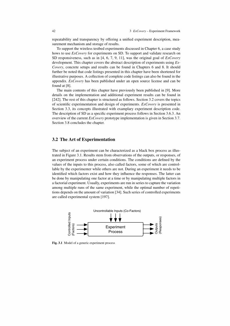
42 3 ExCovery – Experiment Framework
repeatability and transparency by offering a unified experiment description, mea-surement mechanism and storage of results.
To support the wireless testbed experiments discussed in Chapter 6, a case studyhows to use ExCovery for experiments on SD. To support and validate research onSD responsiveness, such as in [4, 6, 7, 9, 11], was the original goal of ExCoverydevelopment. This chapter covers the abstract description of experiments using Ex-Covery, concrete setups and results can be found in Chapters 6 and 8. It shouldfurther be noted that code listings presented in this chapter have been shortened forillustrative purposes. A collection of complete code listings can also be found in theappendix. ExCovery has been published under an open source license and can befound at [8].
The main contents of this chapter have previously been published in [9]. Moredetails on the implementation and additional experiment results can be found in[242]. The rest of this chapter is structured as follows. Section 3.2 covers the topicsof scientific experimentation and design of experiments. ExCovery is presented inSection 3.3, its concepts illustrated with examplary experiment description code.The description of SD as a specific experiment process follows in Section 3.6.3. Anoverview of the current ExCovery prototype implementation is given in Section 3.7.Section 3.8 concludes the chapter.
3.2 The Art of Experimentation
The subject of an experiment can be characterized as a black box process as illus-trated in Figure 3.1. Results stem from observations of the outputs, or responses, ofan experiment process under certain conditions. The conditions are defined by thevalues of the inputs to this process, also called factors, some of which are control-lable by the experimenter while others are not. During an experiment it needs to beidentified which factors exist and how they influence the responses. The latter canbe done by manipulating one factor at a time or by manipulating multiple factors ina factorial experiment. Usually, experiments are run in series to capture the variationamong multiple runs of the same experiment, while the optimal number of repeti-tions depends on the amount of variation [34]. Such series of controlled experimentsare called experimental system [197].
ExperimentProcess
Uncontrollable Inputs (Co-Factors)
Out
puts
(Res
pons
es)
Cont
rolle
d In
puts
(Fac
tors
)
Fig. 3.1 Model of a generic experiment process

3.2 The Art of Experimentation 43
Experiments need to be reliable in a sense that they must be verifiable when re-peated under similar conditions. A sound experiment design must therefore keeprepetition in mind and the publication of experiment data must contain all necessaryinformation to do so. Furthermore, experiments need to fulfill requirements for va-lidity, a concept which is described in more detail in Section 3.2.4. A comprehensiveguide on how to experiment and the caveats of running experiments can be found in[208].
3.2.1 Experiments in Computer Science
The role of experimentation in computer science has been the root of numerous de-bates, for example in [222, 88]. When computer science is seen as an engineeringdiscipline, all subjects of inquiry are synthetic, as created by man. An often ex-pressed opinion is that phenomena in computer science should thus be derived andexplained following the construction of these subjects, instead of observing them asnatural phenomena. However, the complexity of these subjects and their relation-ships in distributed system ever more often prohibits such deduction. Additionally,the subjects of computer science have become part of the world around us and inter-act with it, creating not entirely synthetic hybrids. As such, observation as in naturalsciences can be justified just as the testing of hypotheses to assess and understandman-made systems.
When doing experiments in computer science, challenges exist mainly related toobservation and repetition. It is not always clear which responses to observe andhow to do that in such a way that the observation has no impact on the responseitself. Modern computing systems provide ways to observe tens of thousands ofparameters and observing them – measuring, recording and extracting – has to bedone in the least invasive way. Also, repeating experiments can be difficult due todependence on the original hardware and software platform. Where technology isproceeding at such rapid pace, experiments should be planned as independent aspossible from specific hardware and software revisions they are running on, that is,if the revisions themselves are not the subject of experimentation.
3.2.2 Experiment Factors
Factors are the different sources of variation among individual experiments. Becausethere can be so many factors it is useful to classify them further according to [164].
Treatment factor Any substance or item whose effect on the data is to be studied[74]. It can have continuous values but usually has discrete levels that are to beapplied to study its effect. Treatment factors can be further classified as designfactors, intentionally varied during the experiment, held-constant factors, whose

44 3 ExCovery – Experiment Framework
impact is intentionally neglected by keeping their values fixed and allowed-to-vary factors, known to have a minor influence that can be compensated by ap-plying randomization and replication (see also Section 3.2.4).
Nuisance factor On the other hand, nuisance factors have an unwanted effect onthe output. They can be divided into controllable and uncontrollable nuisance fac-tors. The former, often called blocking factors, can be fixed by the experimenterto reduce their impact on the response. The latter, also called covariates, cannotbe set but their effect can be measured. Minimizing the impact of these effectson the experiment results can be done, for example, doing covariance analysis.Finally, noise factors cause random variations in the responses.
3.2.3 Experiment Design
A treatment is the entire description of what can be applied to the treatment fac-tors of an Experimental Unit (EU), the smallest unit to which such treatment canbe applied [24]. An Observational Unit (OU) then is the smallest unit on which aresponse will be measured. Experiment design defines which treatments are to beobserved on which EUs [74]. Following [116], it can be divided into treatment de-sign, a specification of the treatments used in an experiment, error control design,defining how specified treatments are to be applied to reduce unwanted variations,and sampling and observation design, which decides on the OUs and whether uni-variate or multivariate observations are to be taken.
Experiments tend to be time consuming. Proper experiment design strives tomaximize the gained information per run by optimized structuring of factors andfactor level variations over a required number of runs. This will be expressed in ahigher precision of the response or in an increased significance of factor relation-ships. Reference experiment designs include completely randomized, randomizedblock, full factorial, fractional factorial, screening, response surface method, mix-ture, regression and space filling designs. A thorough explanation of experimentdesigns and for which objectives to apply them can be found in [74, 164].
3.2.4 Experiment Validity
Experiments need to fulfill requirements for internal and external validity. Inter-nal validity demands that causal relationships between factors and responses areverified. External validity deals with the generalization of experiment results. Toimprove the validity of experiments, three interconnected principles are applied.
Replication Increases the number of experiment runs to be able to average outrandom errors and to collect data about the variation in responses. Care has to betaken in the selection of held-constant factors to allow for proper replication.

3.2 The Art of Experimentation 45
Blocking Means partitioning observations into groups, such that observations ineach group are collected under similar conditions [74]. Statistical analysis re-quires that observations are independently distributed random variables [164].
Randomization The assignment of treatments to EUs as well as the temporalorder and spacial choice of multiple runs takes care of the requirement of ran-domization. A design is called completely randomized when all treatment factorscan be randomized. It generally strengthens the external validity if an experimentis run in a diversity of platforms (see also Section 3.2.5).
3.2.5 Experimentation Environment
To carry out the experiments on SD presented in Chapter 6 and 8, the ExCoveryframework has been developed. The core of ExCovery is a formal experiment de-scription that facilitates automated checking, execution and additional features, suchas visualization of experiments. ExCovery is expected to foster experiment repeata-bility, comparability and transparency as it offers a unified experiment description,measurement mechanism and storage of results. The main features of ExCovery arehighlighted in this chapter and focus on the description of the conducted experi-ments and the analysis of their results. More background information on ExCoverycan be found in [9] and [242]. To identify the demands ExCovery addresses, it isnecessary to define what an Experimentation Environment (EE) is and what it needsto provide to an experimenter.
In the context of this work, an EE is defined as a set of tools with the purposeof describing, executing and evaluating experiments on a given subject, using amethodology specific to that subject. The actual setting in which the experimentsand the EE are run is called platform. In general, an EE allows to perform a certainclass of experiments in a controlled environment. It facilitates the identification andmanipulation of factors and the observation of these manipulations on the responses.The amount of possible control depends on the characteristics of the EE. For co-variates, the EE should allow to record them to be considered during analysis at alater stage. To foster the repeatability, correctness and transparency of experiments,an EE should use a well-defined description for setup, execution and evaluation ofexperiments. A common output format for measurements, logs and diverse metainformation should be provided.
Last but not least, an EE should help an experimenter in designing and executingseries of high quality experiments on the topic of interest. Experiments should beinterruptible and resumable. For example, wireless testbeds allow users to experi-ment only in booked timeslots. When time is up an experiment should gracefullystop to be continued at a later stage. Experiments should execute as fast as possible.This is especially necessary for the experiments carried out in Chapter 6 as currentSDPs use very long timeouts for some processes exchanging very few packets. Thismakes it difficult to execute enough repetitions to get reliable and valid results. Fur-thermore, in a distributed environment one has to consider robustness aspects for

46 3 ExCovery – Experiment Framework
the experimentation software itself. It should be able to handle node and connectionfailures, continuing the experiment where possible but stopping it where necessary,alerting the experimenter.
Network Experimentation Environments
ExCovery focuses on experiments to evaluate the dependability of distributed pro-cesses, such as network protocols that enable SD. Thus, it relies on network ex-perimentation platforms like simulators and testbeds or mixed forms of both, forexample virtualized testbeds or simulators with interfaces to real networks or realprotocol implementations.
Simulators are software artifacts that simulate real-world processes by acting ac-cording to an abstract model. They can be discrete event-driven simulators, whichcalculate the state of the simulated object only when its state changes, or real-timesimulators, which calculate the continuous behavior of the simulated object overtime. There also exist mixed forms, for example, where an event-driven simulatoris synchronized to a wall clock. While simulators have a perfect reproducibility ofexperiments, good scalability and generally a reduced execution time, their abstrac-tions often struggle to capture the properties and behavior of real-world distributedsystems [161]. A collection of caveats when simulating real-world effects with com-puter systems is explained in [200]. In this work, when reverting to simulators weused NS-3 [115, 13] which is common in the community.
A testbed on the other hand is made of real network devices. They allow less con-trol over factors but measurements are the result of a realistic interplay of factors.As such, testbeds allow to represent a specific environment, for example a wirelessmesh or a large scale internet network, very well. Testbeds usually provide means tomanage experiment schedules and setup, data acquisition and storage. An approachto unify generic network experimentation across simulators, emulators and testbedsis proposed with NEPI [134, 192], an integration framework for network experi-mentation which creates a common model of experimentation that can be appliedto many physical testbeds as well as to the NS-3 simulator and the netns emulator.Another approach focused on testbeds is Weevil [240], a model-driven experimentframework that was developed to automate large-scale experiments on distributedtestbeds, with several enhancements regarding repeatability and scenario definitionproposed in [241]. However, none of those approaches provides the full chain ofdescription, execution, measurement and storage of experiments as does ExCoverywith comparably low requirements on the platform they run on (see Section 3.3).ExCovery additionally has a special focus on time behavior analysis of networkprotocols, such as SDPs.
Choosing a wireless testbed which fulfills the requirements is no trivial task asbehavior in reality can deviate dramatically from expected behavior. This fact is con-vincingly demonstrated for current testbeds in [161]. To carry out the experimentsneeded for this work in wireless networks, we employed the Distributed EmbeddedSystems (DES) testbed at Freie Universitat Berlin (FUB). The DES testbed provided

3.3 The Experimentation Environment ExCovery 47
the best compromise among usability, availability and versatility. Nodes run a recentversion of the Linux operating system which facilitates software development anddeployment. Second, the DES testbed is regionally close and the staff was alwaysready to provide technical help in unexpected situations. Third, the design of thetestbed and its layout allow the generation of a manifold of different scenarios toexperiment in. Comprehensive background information about the DES testbed canbe found in [100, 101, 36]. In the last years, however, many other wireless testbedshave become available to the community. This is why ExCovery supports the DEStestbed as a first platform, but is not restricted to it, it can be ported to other platformsfor comparison in the future.
3.3 The Experimentation Environment ExCovery
We will now present the main concepts of the proposed experimentation environ-ment ExCovery with its core, the formal abstract description of an experiment usingthe Extensible Markup Language (XML). An XML schema of such a description isprovided with the framework code on request. A version specific to SD as an exper-iment process, which was utilized for the experiments in Chapters 6 and 8 can befound in Appendix A. The description includes definitions of the experiment with itsinput factors, the process to be examined, of fault injections or manipulations anddiverse platform specific and informative declarations. ExCovery further providesa unified measurement concept that determines which and how data are stored forlater analysis. An overview of the different concepts and the experiment work flowis illustrated in Figure 3.2, which shows the different steps when experimenting withExCovery.
In the first preparation step, the experiment is designed by the experimenter fol-lowing guidelines as mentioned in Section 3.2.3. The individual descriptions will beexplained in Section 3.5. Second, platform setup is necessary to prepare the trans-lation of descriptions to the target platform, such as a simulator or a testbed. Thiscould include the deployment of executables and configuration files. The experimentis then executed by the experiment master as specified in the description. Each runis a sequence of actions performed on the participating nodes, described as the mainprocess under evaluation and a set of injected faults or manipulations. The mas-ter and all nodes monitor and record dedicated parameters during each run, suchas raw packet captures and the complete temporal sequence of Experiment Process(EP) actions and events. These data will be saved in a temporary location locally onthe nodes. After experiment execution, the recorded data are collected and condi-tioned so that a common time base for all actions, events and packet measurementsis established. Finally, data are stored into a single results database that contains allconditioned measurement data, created log files and the complete experiment planwith the exact sequence of treatments, as described in Sections 3.4 and 3.4.2).

48 3 ExCovery – Experiment Framework
Desi
gn +
Prep
arat
ion
Meta Description
Experiment Design Description
Experiment Process Description
FaultInjection Description
Environment Manipulation Description
AbstractExperiment Description
Result Repository
Experiment Master
NodeNode
Node NodeNode
Logs
Packets
Events
User-Specified Data
Platform Setup
Exec
utio
n +
Mon
itorin
g
Collection + Conditioning
Stor
age
Platform Specifics
Fig. 3.2 Overview of ExCovery concepts and experiment workflow. [9]
Platform Requirements
To integrate a specific target platform in ExCovery, it must support several features.Most of the features are needed to establish a controllable environment or to com-pensate for missing control and to allow detailed measurements. As such, these aremainly issues for testbeds, such as the DES wireless testbed. Simulators generallycan be integrated with less effort.
Experiment Management
There must be a separate, non-interfering and reliable communication channel be-tween the experiment master and the nodes participating in the EP. In simulators,this is usually provided by a software interface while testbeds need to possess phys-ically separate network interfaces. During experiments, full and privileged access toall nodes is mandatory. The platform needs to cleanly separate concerns of multipleusers.

3.4 Measurement and Storage Concept 49
Connection Control
Full control over the network connections of the individual network nodes is needed.Network interfaces need to support activation and deactivation. Furthermore, itneeds to be possible to manipulate packets sent over these interfaces based on de-fined rules, such as dropping, delaying, reordering, and modifying their content.
Measurement
There must be methods to capture packets with their exact local timestamps and theircomplete and unaltered content. To facilitate a comprehensive subsequent analysis,a packet tracking mechanism is required. In testbeds, this means tracking the routesof packets hop by hop, or attaching unique identifiers to packets [253]. Finally, theplatform needs to support time synchronization among all participating nodes andquantification of the synchronization error.
3.4 Measurement and Storage Concept
This section clarifies the basic observations that are possible using ExCovery, howthey can be observed and how this can help to unify related experiments. ExCov-ery follows the principle of collecting as much data as possible to support diverseanalyses on the same experiment data at later time, emphasizing reusability andrepeatability.
3.4.1 Measurement Data
What data is recorded by ExCovery and how is specified in the following section.Basic recordable data are the results of protocol operations as reflected by statechanges on the participants and network messages sent among participants. ExCov-ery supports a plugin concept to extend these data with custom measurements [242].
Events
State changes on nodes in the context of ExCovery reflect events and occur, for ex-ample, when an experiment run is initialized or when a fault injection is started.Also any defined states of the EP signify events, such as Discovery Request Sentor Discovery Response Received in the case of SD. Events are associated with thenode on which they occur. They contain a local time stamp and may have addi-tional parameters, such as the identifier of the initialized experiment run. To control

50 3 ExCovery – Experiment Framework
the experiment execution, nodes can be synchronized using global events (see alsoSection 3.6).
Packets
Packets are the basic communication data of network protocols. As opposed toevents, single packets are not easily identified: Their location changes as they tra-verse the network, retransmissions and network loops complicate the correct lo-calization at any given time. Packets are recorded to facilitate verification of therecorded event list and to derive statistical connection parameters. A measuredpacket consists of a time stamp, representing the local occurrence of that packet,a unique identifier, a source and destination network address and the packet contentitself.
Time
Events and packets have local time stamps of the node they were measured on. Ex-Covery defines mandatory measurements to be done before each run to estimate thetime difference of each participant to a reference clock. This allows to constructa valid global time line of events and packets, avoiding causal conflicts due to lo-cal clocks deviating between experiment runs. This is especially needed when timesynchronization protocols cannot be used because they interfere with the experimentprocesses.
Topology
To improve repeatability, an extensive description of the network topology is mea-sured. This description includes the local information on each node about its directneighbors and any other known nodes as well as the links between them. For eachlink, the quality as reflected in the Expected Transmission Count (ETX) metric isrecorded (see Section 7.5). This measurement is done at the end of each repeti-tion within a series of experiments. This way, the impact of fault injection or loadgeneration will also be reflected in the routing layer quality metrics. Using thesemeasurements, ExCovery allows to track network dynamics over extended periodsof time.
3.4.2 Storage and Conditioning
ExCovery envisions four levels of storage for experiments, with defined data struc-tures. This allows reusable data access functions among experiments. For more de-

3.4 Measurement and Storage Concept 51
tailed information on data conditioning and the current implementation of the stor-age concept refer to [9], [242].
The first storage level is the abstract experiment description itself, stored in anXML document. This document can be exchanged and loaded for execution andanalysis. The second level is an intermediate storage for all concrete experimentdata: experiment results and the software artifacts used during execution. The sec-ond level storage implementation is flexible and depends mainly on the capabilitiesof the execution platform. ExCovery does not impose a specific storage mechanismbut requires that it is accessible during the subsequent collection and condition-ing phase. Currently, ExCovery uses a special hierarchy on a file system to storesecond level data. Each node has its own temporary storage for recorded data, or-ganized into data belonging to single runs and to the entire experiment. Each logfile and measurement is stored corresponding to a run identifier and associated tothe originating node. Time synchronization measurements are stored on the experi-ment master. Plugins have a separate storage location on the node where the custommeasurements are done.
On the way to the third storage level, data are conditioned by first evaluatingthe synchronization measurements (see Section 3.4.1) and unifying the time base ofall second level measurements. Then, the event list and captured packets are split upinto single data items. Data from the second level plus the experiment description arethen stored into a single package on the third level, which represents one completeexperiment and is preferably stored as a database to unifiy and accelerate data accessand extraction methods. Facilitating exchange of experiments, ExCovery currentlystores the third level in a file based relational SQLite database. This allows to usethe included XML description to recreate the exact run sequence of the experimentand to use SQL to access data stored within the database.
Table 3.1 shows a subset of the tables and their attributes at the third level. Storeddata is classified as either experiment or run based. Run-based data is stored forevery run of the experiment, while experiment-based data is only stored once perexperiment. All run based measurements are identified by a run identifier (ID) anda node ID, which form the primary key of the related entities. A run ID representsone run and a node ID specifies one concrete node by its name.
Table 3.1 Tables and Attributes of Current Storage Concept
Table AttributesExperimentInfo ExpXML, EEVersion, Name, CommentLogs NodeID, LogEEFiles ID, FileExperimentMeasurements ID, NodeID, Name, ContentRunInfos RunID, NodeID, StartTime, TimeDiffExtraRunMeasurements RunID, NodeID, Name, ContentPackets RunID, NodeID, commonTime, srcNodeID, DataEvents RunID, NodeID, commonTime, Type, Parameters

52 3 ExCovery – Experiment Framework
The table ExperimentInfo represents the experiment as a whole and containsonly one tuple made of the abstract experiment description, the version of Ex-Covery and a descriptive name and comment. Logs contains all raw log files andEEFiles the used ExCovery executables. In ExperimentMeasurements, specificnamed measurements are stored that are done once per experiment. As for run baseddata, RunInfos contains for each run and node the start time of the run and the off-set of the node clock to the reference clock. Custom measurements are stored inExtraRunMeasurements. The table Packets contains for each packet the commontime stamp of detection, its originating node and the raw packet data. The Events
table lists all recorded events and their parameters, identified by the run, the originat-ing node and a common time stamp. This schema represents a preliminary approachto store data. Several future improvements are possible, for example by using a di-mensional database model to store experiments in a data warehouse structure.
The fourth level describes the integration of multiple experiments into a singlerepository to facilitate comparison and analysis covering multiple experiments. Todate, this level is not yet implemented in ExCovery.
3.5 Abstract Experiment Description
The core of experiments carried out with ExCovery consists of an abstract descrip-tion in the Extensible Markup Language (XML). For reasons of brevity, this sectionexplains only the most important settings included in the experiment description. Amore thorough listing can be found in [9], [242]. Four main parts are defined in thedescription of experiments:
General This part defines several parameters describing general informationabout the experiment to facilitate categorization, for example the name of the ex-periment, the time it was started or, in the case of this work, the SDP to be used.Figure 3.3 shows a rudimentary general section of an experiment description.Four abstract nodes are to be mapped by the processes described later. Param-eters further classifying the experiment process are advisable as they shall helpin recreating experiment conditions and in making them more transparent. Forbasic experiment classification, two parameters describing the discovery archi-tecture and protocol are defined as key-value pairs. More information about SDarchitectures and protocols can be found in Section 2.2.
Platform The platform definition contains all concrete nodes that take part in theexperiment. Nodes are classified into two types: Actor nodes take part in theprocess under experimentation, for example the discovery process. Environmentnodes take part in the specified environment processes, such as load generationand fault injection. All nodes help with regular routing. Figure 3.4 shows anexemplary platform definition with four actor nodes to carry out the SD operationand five environment nodes (see also Section 3.5.1).
Factors The factor definition contains a list of factors and factor levels whose ef-fect on the results is to be studied. The order of the factors defines how the factor

3.5 Abstract Experiment Description 53
level combinations are applied, with the last factor changing its level most often.Concrete actor nodes are mapped to abstract roles of the EP, such as requestersand responders in the case of discovery. Furthermore, the number of load gener-ators, which are pairs of environment nodes, and the data rate per pair is defined.Also, the number of repetitions of each factor combination is stated as a specialfactor. An exemplary factor definition is listed in Figure 3.5. More information onthe interpretation of factors when executing experiments can be found in Section3.5.2.
Processes This part contains descriptions of experiment processes, executed onlyby specific actor roles and environment processes, which are executed by possiblyall nodes. ExCovery describes processes as series of interdependent actions andevents as detailed in Section 3.6. Due to space constraints, no full description ofthe processes for the discovery actors and environment nodes is shown here. Thefull descriptions can be found in Appendix B.
<experiment_name>just a name</experiment_name><totalnodes>9</totalnodes><abstractnodes><abstractnode id="R0"></abstractnode><abstractnode id="P0"></abstractnode><abstractnode id="P1"></abstractnode><abstractnode id="P2"></abstractnode>
</abstractnodes><sd_level>user</sd_level><sd_protocol>zeroconf</sd_protocol> <!-- may also be "slp" --><sd_arch>2-party</sd_arch>
Fig. 3.3 Rudimentary general section of an experiment description with informative parametersabout discovery process and listing of abstract nodes.
In the following, the individual elements of the abstract description are explained.How exactly they may be used within an experiment description is defined in theXML schema in Appendix A.
Factor Part of the treatment applied to the EU. Consists of a set of levels. Depend-ing on the design, levels are applied One aFter AnoTher (OFAT) or randomized.
List of factors Contains all factors used, sorted. In an OFAT design the first factorvaries least often during execution while the last factor changes every run.
Level Concrete value a factor can take, as input variable to the sub-processes ofeach run. Levels can be of different types. As such, they can control type andduration of fault injections (see Section 3.6.1) or represent mappings of abstractnodes to actors.
Set of levels All levels that should be applied during the experiment. Order ofapplication is determined by the factor definition. There is only a single level ifthe factor should be kept constant during the whole experiment.
Replication factor Parameter defining an integer number of replications to bedone for each treatment.

54 3 ExCovery – Experiment Framework
<platform_specs><description>Nodes to be used during the experiment. Four actors (one↩→ requester, three responders) and five environment nodes for traffic↩→ generation.</description><spec_node_mapping><spec_actor_map abstract_id="R0" id="t9-154" ip="172.18.17.8" /><spec_actor_map abstract_id="P0" id="t9-006" ip="172.18.17.104" /><spec_actor_map abstract_id="P1" id="t9-147" ip="172.18.17.179" /><spec_actor_map abstract_id="P2" id="t9-020" ip="172.18.17.88" /><spec_env_map id="t9-117" ip="172.18.17.52" /><spec_env_map id="t9-k61" ip="172.18.17.92" /><spec_env_map id="t9-169" ip="172.18.17.50" /><spec_env_map id="t9-018" ip="172.18.17.14" /><spec_env_map id="t9-022a" ip="172.18.17.80" /></spec_node_mapping></platform_specs>
Fig. 3.4 Exemplary platform definition for an experiment description. The abstract id allows toidentify abstract nodes for the mapping to actor roles. IP addresses help in filtering the raw capturefiles for packet based analyses.
<factorlist><factor usage="blocking" id="fact_nodes" type="actor_node_map"><description>Mapping of abstract nodes to actor roles of the discovery↩→ process</description><levels><level><actor id="requester"><instance id="0">R0</instance></actor><actor id="responder"><instance id="0">P0</instance><instance id="1">P1</instance><instance id="2">P2</instance></actor></level></levels></factor><factor usage="random" id="fact_pairs" type="int"><description>Number of node pairs for load generation, randomly distributed↩→ in the network</description><levels><level>10</level></levels></factor><factor usage="constant" id="fact_bw" type="int"><description>Datarate per node pair</description><levels><level>100</level><level>500</level></levels></factor><replicationfactor usage="replication" id="fact_replication_id"↩→ type="int">1000</replicationfactor></factorlist>
Fig. 3.5 Exemplary factor definition for an experiment description. The factors are explainedwithin the definition code. The replication factor denotes the number of experiment runs for eachfactor level combination.

3.5 Abstract Experiment Description 55
Abstract node Actor of the EP or of a node specific fault injector. Identified by anode identifier, such as a unique host name.
Environment node A node not participating as actor in any node specific pro-cess. Used e.g. to generate load.
Actor description Process prototype to be executed on one specific actor of theEP. Each abstract node is mapped to one actor description, multiple abstractnodes can instantiate the same actor description.
Experiment process Experiment operation that is to be executed and measured.Consists of actions performed on multiple nodes, synchronized by flow controlfunctions that wait for a certain time or for certain events.
Manipulation process Main part of the treatment. Similar to EPs, represents asequence of faults or impairments that should happen on a node.
Environment manipulation process Like experiment and manipulation processesbut not node specific. Controls environment manipulations such as traffic gener-ation.
3.5.1 Platform Definition
To instantiate an abstract experiment description on a concrete platform, such as awireless testbed, a definition of this platform is required. In this definition, abstractand environment nodes are mapped to concrete, physical nodes of the experimentplatform. ExCovery identifies nodes by their host name and IP address. The hostname should be constant during an experiment run. When an IP addresse changesdue to reconfiguration of a network interface, for example after an injection of sucha fault, an event is generated to signal this.
Figure 3.4 illustrates a compact version of a platform specification. Four actornodes and five environment nodes exist. Actor nodes map to an abstract node id thathas been previously defined (see Figure 3.3). All nodes have a unique identifier anda network address that can later be used to analyze the recorded event and packetlists.
3.5.2 Experiment Execution from Factor Definition
To execute the overall experiment and its individual runs from the abstract descrip-tion, ExCovery generates treatment plans from replications, the factors and theirlevels. Plans are OFAT if no custom factor level variation plan is given. The variousrandom values used in ExCovery are generated using pseudo-random generators.This allows for perfect repeatability of random sequences when initialized with thesame seed. Which seed is used for initialization is clearly defined in the experimentdescription so that all random sequences can be reproduced. Software for the designof experiments exists that can help with the generation of such treatment plans, this

56 3 ExCovery – Experiment Framework
is why a specific plan generator is outside the scope of this work. However, ExCov-ery supports plan generators by providing all necessities, such as factor, level andrepetition representations.
ExCovery uses four internal functions for the experiment flow. Experiments areinitialized by calling experiment init on every participant, which takes care ofthe necessary preparations before all individual experiment runs. Each run is theninitialized by run init. There further exist the respective exit functions run exit
and experiment exit.Figure 3.5 shows the definition of several factors and their levels. It maps the
abstract nodes listed in the general section of the description (see Figure 3.3) to actorroles requester and responder, defines 10 node pairs for load generation whichwill first have a data rate of 100, then 500 kbit/s each. Each factor combination willbe run 1000 times as stated by the replication factor. Since there is only one nodemapping and one factor level for the load generation, there will be 1000 runs foreach data rate.
Experiment Phases
ExCovery is designed to provide a consistent state for each repetition and to min-imize effects of any process not described in the experiment description, includ-ing its own processes. Each run consists of a preparation phase, an execution ormeasurement phase which is the core of the experiment and a cleanup phase. Dur-ing preparation, the whole environment of the EP must be reset to a defined initialworking condition. Software agents are initialized. In testbeds, for example, networkpackets generated in previous runs must be dropped on all participants. Preliminarymeasurements can be done to compensate for incomplete control over the environ-ment, such as clock offsets for all participants. During the measurement phase, onlythe processes defined in the experiment description are executed and their effectsrecorded by specified nodes. Only after completing all runs these measurements areimported from their temporary directories, conditioned to contain a globally validtimestamp and written to a database. The database represents one full experimentand can be shared to allow transparent reusability and repeatability. It includes theexperiment description, logged events and packets of the described processes anddiverse information about the state of the testbed itself. The latter can be used tofurther decrease the effect of external processes. All steps will be repeated duringeach run, this has to be considered when estimating the total time an experimentneeds to finish.
3.6 Process Description
ExCovery provides common mechanisms to control execution of the defined pro-cesses. Two types of processes can be differentiated, depending on whether they

3.6 Process Description 57
relate to abstract nodes or to the environment. Abstract node processes are mappedto real nodes during experiment execution, such as protocol actions or fault injec-tion processes. Environment processes are performed by all nodes, such as drop-ping packets on all network interfaces to reset the environment. Every process isdescribed as a sequence of actions. Processes run concurrently so one needs to con-sider timing and desired or necessary dependencies. ExCovery defines methods forsynchronization to provide basic flow control.
wait for time Process waits for a fixed delay in seconds.wait for event Process waits until the specified event is registered on any partic-
ipant. An event can be specified by its name, location and any of its parameters.The location is either a single abstract node or a subset of nodes specified by anactor role. Event parameters can be of diverse types. If omitted, they default to”any“. A time-out in seconds can be set.
wait marker Creates a time stamp used by the next wait for event call, whichconsiders only events occurring after that time stamp.
event flag Used to create local events to let process actions depend directly oneach other.
Besides these flow control functions, there are process specific actions, environ-ment actions and manipulation actions. Each action can have a list of parameters,allowing the description of manifold scenarios. In Section 3.6.3, SD as an EP isdescribed to illustrate this. Manipulation processes are described in Section 3.6.2.
Figure 3.6 shows a code fragment where the different processes are defined, with-out the actual sequences of actions that will be described later. Among the nodeprocesses, the role responder is defined and as possible actor nodes, the abstractnodes fact nodes from the factor list are referenced. Environment processes do notneed a definition of nodes.
<processes max_run_time=120><env_process><!-- list of environment process actions -->
</env_process><node_processes name="..."><process_parameters><actor_node_map><factorref id="fact_nodes"/>
</actor_node_map></process_parameters><actor id="responder" name="SM"><!-- list of node process actions -->
</actor></node_processes>
</processes>
Fig. 3.6 Template for the description of node and environment processes.

58 3 ExCovery – Experiment Framework
3.6.1 Manipulation Processes
ExCovery has a concept for intentional manipulations done on participant nodesand on their network environment. Manipulations cover direct fault injections thatcause failures in a target area. Fault provocation is used when direct injection isnot desirable or possible and characterizes actions that are known to provoke faultsin a target area. The main faults considered are communication faults. ExCoveryprovides a simplified fault model to allow for the description of basic fault behav-ior with a set of common parameters. Fault injection processes can have commonparameters describing their temporal behavior: duration, ratio and randomseed.
Duration Specifies the amount of time a fault should be applied to the target.Ratio Specifies a percentage of a given period in which a fault is active. The fault
is active in one continuous blockRandomseed The fault activation time in the period is chosen randomly using
this parameter as seed.
Fault Injections
Mechanisms for fault injection are explained in the following. In addition to thecommon parameters, injections can have custom parameters to further define theirbehavior. It should be noted that all injected faults add up to already existing com-munication faults in the target platform. Also, whenever the term packet is used itrefers to packets belonging to the EP.
Interface fault No messages are transmitted or received on the specified interfacein the specified direction as long as this fault is active. Direction can be receive,transmit, both, or chosen randomly.
Message loss Defines probability for every packet to be dropped. Direction isanalogous to the interface fault.
Message delay Applies a constant delay to every packet.Path loss, path delay Path loss and delay are message loss and delay faults, se-
lectively affecting only the communication between the target and a given secondnode.
Environment Manipulations
Environment manipulations are applied on a global level and involve possibly allspecified environment nodes. Manipulations include the previously defined fault in-jections. Additionally, the following manipulations can be applied.
Traffic generator Creates network load between a given number of node pairs.Each pair bidirectionally communicates at a given data rate (see also Figure 3.5).

3.6 Process Description 59
Pairs can be randomly chosen from the acting nodes, non-acting nodes or allnodes. Pairs vary between runs as determined by a switch amount parameter.
Drop all packets All experiment nodes stop receiving, sending and forwardingEP packets.
Every fault injection and environment manipulation but the traffic generator isstarted only once and without a given duration, needs to be explicitly stopped. Givenis just the default list supported by ExCovery. ExCovery provides also a genericfunction with an arbitrary list of parameters that are given to the acting nodes to beexecuted [242]. However, an experimenter should preferably extend ExCovery bydefining a plugin with new functions and their implementation.
3.6.2 Manipulation Process Description
Manipulation processes are defined in the experiment description as a series of ac-tions and events. This list is executed sequentially and can contain flow controlfunctions as described in Section 3.6. A node manipulation process is created foreach abstract node it is specified for while the environment manipulation processis implicitely supported on all nodes. The specific actions activate or deactivate thefaults and manipulations. One event is generated by each action to signal its startor stop, respectively. Parameters of these actions can be constant or varied duringexperiment execution. Variation is realized by references to factors instead of fixedvalues.
Start interface fault Starts interface fault with the given parameters. Generatesfault start interface event.
Start fault message loss Starts message loss fault with the given parameters.Generates fault start messageloss event.
Start fault message delay Starts message delay fault with the given parameters.Generates fault start messagedelay event.
Start traffic generator Traffic generator is started by this action.Start dropping all packets Starts the corresponding manipulation in order to
purge all experiment process packets from the network.
The manipulation actions can be used to extend the EP description or to defineseparate manipulation processes. This depends on whether manipulations shall besynchronous with the EP or autonomous. Figure 3.7 shows a shortened listing ofa traffic generation process. After generating a ready to init event, it uses thefactors from Figure 3.5 to choose and configure traffic generation by a set of envi-ronment nodes, switching one pair of nodes in every run. The manipulation remainsactive until done is registered.

60 3 ExCovery – Experiment Framework
<env_process><env_actions><event_flag><value>ready_to_init</value>
</event_flag><env_traffic_start><bw><factorref id="fact_bw" />
</bw><choice>0</choice><!-- this causes identical randomization in replications --><random_switch_amount>1</random_switch_amount><random_switch_seed><factorref id="fact_replication_id" />
</random_switch_seed><random_pairs><factorref id="fact_pairs" />
</random_pairs><random_seed><factorref id="fact_pairs"/>
</random_seed></env_traffic_start><wait_for_event><event_dependency>done</event_dependency>
</wait_for_event><env_traffic_stop />
</env_actions></env_process>
Fig. 3.7 Illustrative example of environment process for traffic generation.
3.6.3 Experiment Process Description
Remaining is a description of the main experiment process, whose events and pack-ets are to be observed and measured. The description provides a temporal and causalsequence of actions on the participating nodes as introduced in Section 2.2, facili-tating flow control functions from Section 3.6. In line with the topic of this work,we will explain how to describe generic SD as an EP to be used within ExCovery, tosupport the experiments in Chapters 6 and 8. The description can contain actors forservice providers, service clients and service registries. For reasons of brevity, theseroles will be referred to as SM, SU and SCM, which is in line with the terminologyused in [70]. For each actor a number of instances can be created to represent allparticipants of the SD process.
The model developed in [70] defines a set of main operations for a generic SDprocess, namely “Configuration Discovery and Monitoring”, “Registrations and Ex-tension”, “Service-Description Discovery and Monitoring”, and “Variable Discov-ery and Monitoring”. These will be considered in the abstract SD process descrip-tion, with an optional list of parameters to define specific variants. The descriptiondoes not intend to model a Service Discovery Protocol (SDP) specific behavior indetail, but to give an abstract description of a SD scenario. The details of executingthe description are left to the SDP implementation, so that multiple implementationswhich adhere to the same SD concepts can be compared in experiments. However,

3.6 Process Description 61
the executing SDPs are allowed to generate custom events which will be recordedby ExCovery. Actions that can be executed on participating SD nodes are describedas follows.
Init SD Mandatory action to allow participation of a node in the SD. Repre-sents “Configuration Discovery and Monitoring”. Discoverable items such andscopes and SCMs are discovered and a unique identity is established on eachnode. This action reads as parameter the role as either SCM, SU or SM. Op-tional custom parameters further configure the used SDP. When the SCM pa-rameter is used, the node generates a scm started event. If an SM registersits service on an SCM node, a scm registration add event is generated withthe registering node’s identification as parameter. Analogously, when a registra-tion is revoked or changed, the respective events scm registration del andscm registration upd are generated. In a hybrid architecture, SU and SMagents keep looking for SCMs and emit scm found events when a SCM hasbeen discovered. When SD initialization is complete, sd init done is emitted.
Exit SD Stops a previously started role and all assigned searches and publishings,emitting sd exit done upon completion. To participate again in the SD process,a node needs to re-run init.
Start searching SU and SM nodes initiate a continuous SD process for a givenservice type, generating the event sd start search. Refers to the group of“Service-Description Discovery and Monitoring” functions. ExCovery does notdistinguish among passive, aggressive, or directed discovery (using an SCM).A service is considered discovered when its complete description has been re-ceived. The event sd service add will be emitted with the found service’s iden-tifier as parameter. Analogously, when a service becomes unavailable, the eventsd service del is generated
Stop searching A previously started search is stopped and event sd stop search
generated. Includes de-registration of any notification request on SCMs.Start publishing Starts publishing an instance of a given service type, generating
a sd start publish event. Refers to the group of “Registrations and Extension”functions, such as registration on a SCM.
Stop publishing Gracefully stops publishing a given service type. Comprises fur-ther actions like aggressively sending revocation messages or SCM de-registration.Generates sd stop publish event upon completion.
Update publication Updates a previously published service description. Cov-ers underlying functions related to registration on SCMs. Generates an eventsd service upd with the service identifier as parameter before the update isexecuted.
An example SD scenario depicted in Figure 3.8 shows a single active SD in atwo-party architecture with a timeline for each actor SU1 and SM1. Actions areshown as white circles, events as black circles. Unlabeled events inherit the labelof the preceding action. In the preparation phase, SU and SM initialize themselves.This phase ends a fixed time after sd start publish from SM1 is registered, tolet unsolicited announcements of SM1 pass. SU1 then starts a search, beginning the

62 3 ExCovery – Experiment Framework
execution phase. After a time tR the service is discovered and sd service add isgenerated on SU1. The scenario finishes here, in the clean-up phase searches andpublications are stopped and the SD system shut down.
SM1
SU1
t
sd_init
sd_init
sd_start_publish
sd_start_searchsd_service_add(SM1)
sd_stop_search
sd_stop_publish
sd_exit
sd_exit
Preparation Execution Clean-Up
tR
Fig. 3.8 Visualization of a one-shot discovery process.
Figures 3.9 and 3.10 show descriptions of two-party SD processes for SU andSM roles using the introduced actions and events. The SM role in Figure 3.9 basi-cally starts publishing and continues until a done event is registered. The SU role inFigure 3.10 waits first for all SMs to emit their sd start publish event, next forthe environment to register the ready to init event. It will then start searching andfinish either when all SMs have been discovered, having generated their respectivesd service add events or when the deadline of 30 seconds has been reached. Ineither case, done is generated and the clean-up phase begins.
<actor id="actor0" name="SM"><sd_actions><sd_init /><sd_start_publish /><wait_for_event><event_dependency>"done"</event_dependency>
</wait_for_event><sd_stop_publish /><sd_exit />
</sd_actions></actor>
Fig. 3.9 SD process in a two-party architecture. Publisher role.
The code listings of all processes in this section have been deliberately shortenedfor reasons of readability. Full versions can be found in Appendix B.

3.7 Prototype Implementation 63
<actor id="actor1" name="SU"><sd_actions><wait_for_event><from_dependency><node actor="actor0" instance="all"/>
</from_dependency><event_dependency>"sd_start_publish"</event_dependency>
</wait_for_event><wait_for_event><event_dependency>"ready_to_init"</event_dependency>
</wait_for_event><sd_init /><wait_marker /><sd_start_search /><wait_for_event><from_dependency><node actor="actor1" instance="all"/></from_dependency><event_dependency>"sd_service_add"</event_dependency><param_dependency><node actor="actor0" instance="all"/></param_dependency><timeout>"30"</timeout>
</wait_for_event><event_flag><value>"done"</value></event_flag><sd_stop_search /><sd_exit />
</sd_actions></actor>
Fig. 3.10 SD processes in a two-party architecture. Requester role.
3.7 Prototype Implementation
An ExCovery prototype has been implemented using the Python programming lan-guage [191] with the aim of being reusable on diverse platforms. It abstracts thehandling of the XML experiment description and the resulting run sequence andparameter variations in separate classes that can be instantiated by programs to an-alyze, visualize, trace or export experiment related data.
Some requirements must be met to reuse this implementation in addition to allrequirements mentioned in Section 3.3. For testbed platforms, several additionalrequirements for the software packages exist. Nodes need to run the Linux operatingsystem with a kernel of version 2.6.34 or higher, which was released on May 16,2010. Packet capturing software for the pcap format should be available as wellas the components of the netfilter software. Privileged access is mandatory on allparticipating nodes. The current ExCovery implementation further depends on thesoftware tools tc, iptables, route, kill, killall, traceroute and tshark. All of these arebroadly used standard tools on Linux systems.
As the first platform, ExCovery supports the wireless DES testbed at Freie Uni-versitat Berlin [36]. An implementation for the SD process in Section 3.6.3 ex-ists using the Zeroconf SDP [55, 54, 53] and the Service Location Protocol (SLP)[103, 106]. This section gives a quick overview of the prototype, a comprehensivedescription of the implementation can be found in [242, 61].

64 3 ExCovery – Experiment Framework
Software Components
In accordance to the developed concepts the prototype is composed of one control-ling entity (master) and a set of controlled entities (nodes) as depicted in Figures 3.2and 3.11. Master and nodes are connected in a centralized client-server architecturewith a dedicated communication channel. They communicate synchronously usingExtensible Markup Language Remote Procedure Calls (XML-RPC) [244].
ExperiMasterExperiMasterNodeManagerExperiMasterExperiment
Process Threads
Fault Threads
Environment Thread
Node Objects
Event Handler
RPC Interface
Event Generator
Experiment Process Handler
Fault Handler
Environment Handler
Management Functions
ping
avahi
tshark
iptables
route
traceroute
Fig. 3.11 Execution components of the provided implementation, here only for Zeroconf.
The controlling ExperiMaster maintains a list of objects corresponding to theactive nodes in the experiment on which actions will be executed. A node objectpresents the functions of one node to the master program via XMLRPC and useslocking to allow only one access at a time. Which action is executed at which timeis specified in process descriptions loaded from the experiment description file. Themaster creates an EP thread and a fault thread for each abstract node in the descrip-tion. A single thread is created for the environment manipulations. The actions per-formed by this thread and the management actions performed by the main programcan be executed concurrently on all nodes.
The NodeManager is the central component of the nodes participating in experi-ments. It handles Remote Procedure Calls (RPCs) from ExperiMaster. Basically, theNodeManager provides an interface to the ExperiMaster. Components on a node usethe event generator to signal the occurrence of events, as defined in Section 3.4.1.Basic procedures exposed via RPC are actions for management, fault injection, en-vironment manipulation and the EP actions as defined in Sections 3.3 and 3.6.3. Theimplementation of these functions can be delegated to sub-components, e.g., the EPactions in the context of this work refer to SD actions that are implemented by theAvahi [22] software package in the case of Zeroconf. For SLP, the reference imple-mentation provided by OpenSLP project group [176] is used by means of a Pythonwrapper.
To allow analysis of properties outside the scope of the ExCovery processes, forexample packet loss and delay, a network packet tagger is provided. It remains run-ning in the background on each node. The tagger adds an option to the header of eachselected IP packet and writes a 16 bit identifier to it, incrementing the identifier with

3.8 Conclusion 65
each packet. This approach can cause problems when IP packets are fragmented,due to the packet size being larger than the Maximum Transmission Unit (MTU) ofthe network. In the context of this work, however, SD packet sizes used for testingare generally far below the MTU. Additionally, ExCovery includes a set of Pythonscripts to collect, condition and store experiment results in a database.
The presented concept and implementation generally support multiple SDPs.They need to provide a Linux implementation which provides an interface to fun-damental SDP operations, as represented by the actions in Section 3.6.3. For theprototype, the Zeroconf SDP suite Avahi [22] was modified to allow the associationof request and response pairs. This allows analysis of response times not only atthe SD operation level (tR in Figure 3.8) but at the level of individual SD requestand response packets, which by default is not supported in Zeroconf SDPs. Theseresponse times are different when packets are being lost and requests are retried.Zeroconf is based on multicast DNS [54] and the ID field of the used DNS recordswas chosen to identify responses to a request. This field is suitable and least invasivebecause it “must be ignored on reception” and queries “should not” use the ID field.The identifier is initialised with a random value in each run and then incrementedfor each retransmission and each new query. A set of functions exist for extractionand analysis of event and packet based metrics.
A set of specific analysis functions was added to the framework code as pre-sented in [9] to support the results presented in Sections 6.5 and 6.4. Additionally,diverse enhancements were developed to improve monitoring during execution ofexperiments, given the long durations of the individual experiments. Finally, theframework code for the execution of experiments was redesigned to reduce the du-ration of experiments, especially when they are resumed after partial completion.Since they are not the focus of this work, the implementation of these changes willnot be discussed in detail.
3.8 Conclusion
This concludes the presentation of the ExCovery framework. ExCovery has beentried and refined in a manifold of SD dependability experiments over the last twoyears that were carried out on the wireless DES testbed at Freie Universitat Berlin.Specifically, ExCovery was developed for the experiments on Service Discovery(SD), which are presented in Chapters 6 and 8. The described abstract descriptionof SD as experiment process was used in those experiments.


Part IIUser-Perceived Service Availability

Service-Oriented Architecture (SOA) has emerged as an approach to master grow-ing system complexity by proposing services as basic building elements of systemdesign. However, it remains difficult to evaluate dependability of such distributedand heterogeneous functionality as it depends highly on the properties of the en-abling Information and Communications Technology (ICT) infrastructure. This isespecially true for the user-perceived dependability of a specific pair service clientand provider as every pair may utilize different ICT components.
In Chapter 4, we provide a model for the description of ICT components andtheir non-functional properties based on the Unified Modeling Language (UML).Given a service description, a network topology model and a pair service client andprovider, we propose a methodology to automatically identify relevant ICT compo-nents and generate a User-Perceived Service Infrastructure Model (UPSIM). We fur-ther provide a model-driven methodology to automatically create availability mod-els of such views, called User-Perceived Service Availability Models (UPSAM). Themethodology supports the generation of different availability models, exemplarilyproviding reliability block diagrams and fault-trees. These can be used to calculateuser-perceived steady-state and instantaneous service availability. For instantaneousavailability evaluation, the age of the ICT components, the order and time of theirusage during service provision are taken into account, providing a proper conceptof service time.
Chapter 5 demonstrates the feasibility of the methodology by applying it to partsof the service network infrastructure at University of Lugano (USI), Switzerland.We then show how this methodology can be used to facilitate user-perceived servicedependability analysis. Using the UPSAM, we calculate the availability of an exem-plary mail service in diverse scenarios. We conclude this part by discussing furtherapplications of the methodology and explaining how to combine it with the servicediscovery models in Chapter 7.

Chapter 4Modeling User-Perceived Service Dependability
Abstract This chapter presents an approach to generate models for the evaluationof user-perceived service properties. It provides a model for the description of a net-work of ICT components and their non-functional properties based on the UnifiedModeling Language (UML). Given a set of input models that describe the servicenetwork topology, its services and actors, the proposed methodology automaticallyidentifies relevant ICT components and generates a User-Perceived Service Infras-tructure Model (UPSIM) which can be further transformed into User-Perceived Ser-vice Availability Models (UPSAMs) for steady-state and instantaneous availabilityanalysis. So far, the methodology can create Reliability Block Diagrams (RBDs) andFault Trees (FTs). How these models can be utilized is demonstrated in case studiesin Chapter 5.
4.1 Introduction
This chapter builds on and combines previously published work on the topic whichis described in the following. In order to assess the service dependability from dif-ferent user perspectives, an extraction of relevant network parts is presented in [2].Given a model of the network topology, a service description and a pair service re-quester and provider, a model-to-model transformation is applied to obtain a User-Perceived Service Infrastructure Model (UPSIM) as in Definition 1.2. The approachin [2] uses a subset of Unified Modeling Language (UML) [170] elements as wellas UML profiles and stereotypes [171] to impose specific dependability-related at-tributes to ICT components. The ICT infrastructure and services are modeled in-dependently using UML object and activity diagrams, respectively. Then, a mech-anism is used to project the properties of ICT components to services through anXML mapping that correlates their respective models. The methodology in [2] isbased on the work by Milanovic et al. in [156, 157], which provides the core con-cepts of transforming the three dimensions service, infrastructure and actors into
69

70 4 User-Perceived Service Availability
availability models of the service. More background information about this workcan be found in Section 2.3.2.
In [5], a methodology is presented that provides a UML availability profile toobtain as output instead of an UPSIM a specific availability model expressed asReliability Block Diagram (RBD) to evaluate service availability for different userperspectives. The case study in [5] uses an implementation of that methodologythat is extensively described in [165]. Extending [2] and [5] with a time dimensionhas been done in [12] to support instantaneous service availability evaluation, theprobability of a service to be available at a specific point in time. The infrastructuremodel from [2] is extended to include all ICT components, their failure and repairrates and deployment times. The mapping contains concrete ICT components for theservice requester and provider, including possibly redundant components and theirexpected duration of usage. Using these models, the methodology automaticallygenerates an availability model from those parts of the ICT infrastructure neededduring service provision for the specified user-perceived view. The implementationof this approach is described in [196]. This provides a basic but solid concept ofservice time, an thus allows for true instantaneous availability evaluation. This willbecome even more important when variable and dependent failure and repair ratesare introduced. In [157], although instantaneous availability is calculated, all com-ponents are considered to have been deployed at the same time. Additionally, theservice execution has no duration but happens in one instant of time. The approachin [157] is thus most suitable for steady-state evaluation.
The remainder of the chapter is organized as follows. Section 4.2 defines the in-put models to be used in the service dependability evaluation. The methodology toevaluate user-perceived service dependability is presented in Section 4.3. Section4.4 describes how to use this methodology to generate availability models. In chap-ter 5, the feasibility of the approach is demonstrated in representative case studiesby applying it to an exemplary services within parts of the service network infras-tructure of University of Lugano, Switzerland.
4.2 Model Specification
The methodology consists of generating a UPSIM respectively UPSAM from a ser-vice description, a network topology and a mapping between them. The UPSAMis then evaluated using an external tool for availability analysis. In this section, thedifferent types of input models are defined and explained.
ICT infrastructures are able to support a variety of services, while a single servicedescription can be similarly applied to a diversity of networks. For this reason, thepresented methodology supports independent modeling of infrastructure and ser-vices, relying on a third model to provide a relation between them. This approachimplies also that changes on the network topology or service description should bereflected only in their respective models. Our approach uses a subset of UML ele-ments as it is standardized, easily expandable, well supported by numerous tools and

4.2 Model Specification 71
thus, widely accepted in both industry and academia. Moreover, UML profiles andstereotypes are applied to impose specific attributes to ICT components, resulting ina coherent model with a standardized description:
• Class diagrams are used to describe structural units of the network (e.g.: routers,clients, servers), their properties and relations in distinct classes.
• Object diagrams describe a deployed network structure/topology composed ofclass instances, namely objects with all properties of the parent class, and linksas instances of their relations. Object diagrams are used to describe both thecomplete network structure as well as the UPSIM.
• Activity diagrams are used for the service description and represent the serviceas a flow of actions.
Figure 4.1 depicts the context of a UPSIM as a UML class diagram. The follow-ing subsections explain the different parts of the diagram in detail.
1
*
1
*
1
*
1
*
2
1
1
1
* 2
1*
User-perceived Service Infrastructure Context
Service Mapping Pair
atomic service:Atomic Servicerequester:Componentprovider:Component
ICT Infrastructure
Atomic Service Composite Service
Connector Device
ICT Component
Service
* *
Fig. 4.1 Context of a user-perceived service infrastructure model.
4.2.1 ICT Infrastructure Model
A network topology can be represented as a bidirectional graph, in which networkdevices and their links are respectively characterized by nodes and edges. But inpractice, service dependability rests upon the characteristics of individual compo-nents and networks are generally composed of heterogeneous nodes. This is why in

72 4 User-Perceived Service Availability
opposition to graphs, a separate model would better represent the individual charac-teristics of network components.
The class ICT infrastructure in the left part of Figure 4.1 aggregates a set ofinterconnected ICT components. Network nodes and the communication betweenthem exhibit very distinct properties. For this reason, ICT components are subdi-vided into Device and Connector types. Following standard UML notation, Figure4.1 shows that every Connector must be associated to two Devices, which may haveany number of Connectors. Devices and Connectors are respectively modeled asclasses and associations in a UML class diagram. The ICT infrastructure model isthen presented in a UML object diagram, where network nodes are instance speci-fications of those classes, and communication is represented by the correspondinglinks, which are instances of associations. To ensure that two different instancesof the same class also have the same properties, every class may only have staticattributes.
The same set of attributes can be applied to common model elements throughprofiles [171] to facilitate dependability analysis that requires specific properties tobe present for each model element. A stereotype containing these specific propertiescan be employed to guarantee that every ICT component inherits them and thus,meets the requirements of the analysis. Following this approach, we provide anavailability profile, which is depicted in Figure 4.2. Focusing on both steady-stateand instantaneous availability (see Section 2.3.1), the profile includes the stereotypeattributes (1) failure rate, (2) repair rate and (3) component deployment time, atwhich a component is expected to have its maximum availability. Although anydate and time format could be applied, epoch time has been chosen for deploymenttime to simplify subsequent steps. Additionally, the redundant components propertyspecifies internal redundancy, which can be used to implicitly define a large set ofICT components into a single object in the infrastructure model. ICT componentsare divided into devices and links and are represented in the UML class diagram inFigure 4.2 as classes and associations, respectively.
<<Stereotype>>Component
failureRate: RealrepairRate: RealdeploymentTime: IntegerredundantComponents: Integer
<<Stereotype>>Device
<<Stereotype>>Connector
<<metaclass>>Class
<<metaclass>>Association
Fig. 4.2 Elementary availability profile
Furthermore, a network profile (see Figure 4.3) has been developed to guaran-tee the uniformity of the infrastructure. It defines an abstract stereotype NetworkDevice to capture common properties of identified network components: Router,

4.2 Model Specification 73
Switch, Printer and Computer. The latter one is abstract and specializes into Clientand Server. Communication is a stereotype dedicated to the association betweenclasses, and has channel and throughput attributes. In practice, it corresponds tocommunication links between devices. With this profile, a set of attributes can con-sistently be imposed to stereotyped classes for later model transformation. Albeitonly an illustrative representation in this case study, the network profile of Figure4.3 can support a variety of attributes depending on the application.
<<metaclass>>Class
<<Stereotype>>Client
<<Stereotype>>Server
<<Stereotype>>Network Device
manufacturer:Stringmodel:String
<<Stereotype>>Computer
processor:String
<<Stereotype>>Router
<<Stereotype>>Switch
<<Stereotype>>Printer
<<Stereotype>>Communication
channel:Stringthroughput:Real
<<metaclass>>Association
Fig. 4.3 Network profile with types of elements and their basic properties.
4.2.2 Service Model
Services in the context of this work are described as a sequence of complex ac-tions provided by a composition of atomic service instances. Composite servicesare modeled with UML activity diagrams using atomic services as building blocks,as depicted in the right part of Figure 4.1. A composite service consists of initialand final nodes, atomic services and join and fork figures. Figure 4.4 presents theUML activity diagram of a simple composite service. It is assumed that each atomicservice is being executed – in series or in parallel. In this particular diagram, atomicservices A and B are executed in parallel. Instead of using decision nodes, separatedecision branches are modeled as separate services.
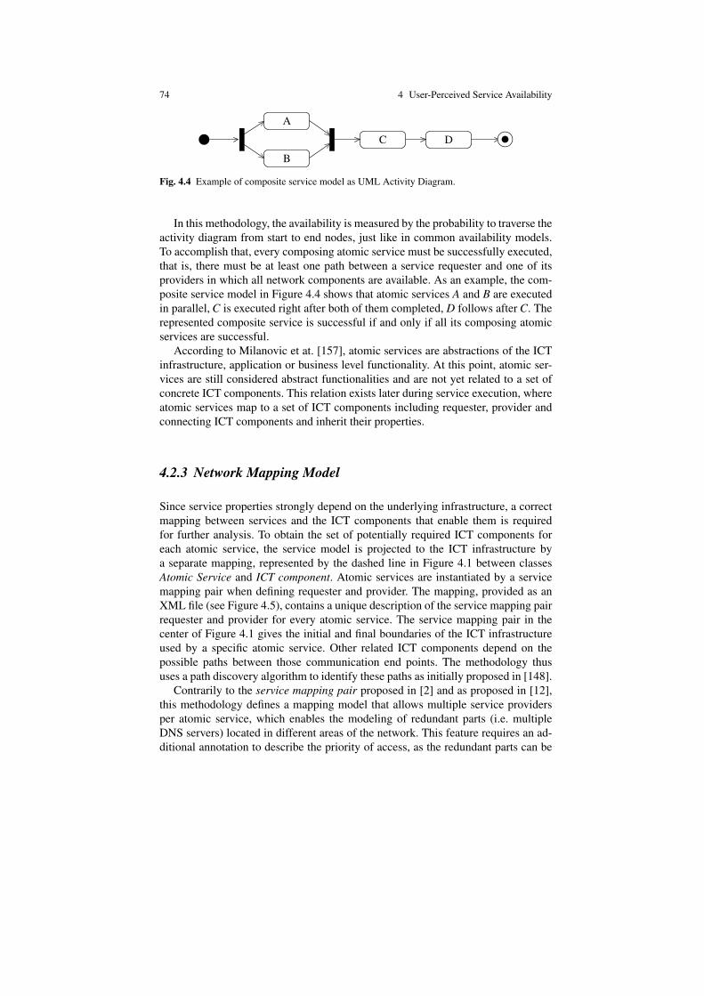
74 4 User-Perceived Service Availability
A
B
C D
Fig. 4.4 Example of composite service model as UML Activity Diagram.
In this methodology, the availability is measured by the probability to traverse theactivity diagram from start to end nodes, just like in common availability models.To accomplish that, every composing atomic service must be successfully executed,that is, there must be at least one path between a service requester and one of itsproviders in which all network components are available. As an example, the com-posite service model in Figure 4.4 shows that atomic services A and B are executedin parallel, C is executed right after both of them completed, D follows after C. Therepresented composite service is successful if and only if all its composing atomicservices are successful.
According to Milanovic et at. [157], atomic services are abstractions of the ICTinfrastructure, application or business level functionality. At this point, atomic ser-vices are still considered abstract functionalities and are not yet related to a set ofconcrete ICT components. This relation exists later during service execution, whereatomic services map to a set of ICT components including requester, provider andconnecting ICT components and inherit their properties.
4.2.3 Network Mapping Model
Since service properties strongly depend on the underlying infrastructure, a correctmapping between services and the ICT components that enable them is requiredfor further analysis. To obtain the set of potentially required ICT components foreach atomic service, the service model is projected to the ICT infrastructure bya separate mapping, represented by the dashed line in Figure 4.1 between classesAtomic Service and ICT component. Atomic services are instantiated by a servicemapping pair when defining requester and provider. The mapping, provided as anXML file (see Figure 4.5), contains a unique description of the service mapping pairrequester and provider for every atomic service. The service mapping pair in thecenter of Figure 4.1 gives the initial and final boundaries of the ICT infrastructureused by a specific atomic service. Other related ICT components depend on thepossible paths between those communication end points. The methodology thususes a path discovery algorithm to identify these paths as initially proposed in [148].
Contrarily to the service mapping pair proposed in [2] and as proposed in [12],this methodology defines a mapping model that allows multiple service providersper atomic service, which enables the modeling of redundant parts (i.e. multipleDNS servers) located in different areas of the network. This feature requires an ad-ditional annotation to describe the priority of access, as the redundant parts can be

4.2 Model Specification 75
<atomicservice id="A"><requester id="req1"></requester><provider id="prov1"></provider>
</atomicservice>
Fig. 4.5 Example of the XML code representing the mapping of a single atomic service.
accessed in parallel or in series after an eventual failure. For the latter case, fur-ther annotations are needed to define serial access times of redundant components.Additionally, this methodology supports redundancy modeling using independentcomponents with possibly different properties, instead of identical replicas as in [2].Service and infrastructure descriptions are time-independent and, alone, are not ableto provide an estimated execution time for atomic services. This becomes instead aparameter of the mapping. Having such information, it is possible to estimate forwhich interval each atomic service availability should be evaluated. The servicemodel (see Section 4.2.1) plays an important role by describing which atomic ser-vices are executed in parallel or in series.
An example of the enhanced mapping model is shown in Figure 4.6. Multipleproviders within an atomic service description are always considered to be redun-dant, that is, at least one of the listed instances must be available for the requesterto achieve a successful service provision. Every instance may be able to provide theatomic service with a different estimated duration in seconds, and the priority (0being the highest) plays a role for the definition of start and end execution times foreach instance access.
<atomicservice id="C" requester="req1" timeout="10"><provider="prov1" duration="3" priority="0"><provider="prov2" duration="4" priority="1"><provider="prov3" duration="8" priority="1">
</atomicservice>
Fig. 4.6 Mapping of atomic service with parameters for instantaneous availability evaluation.
In the example of Figure 4.6, three providers prov1, prov2, prov3 are able todeliver a specified atomic service C to the requester req1. Supposing this atomicservice is invoked at time t = 0s, the example models the following behavior: com-ponent req1 requests a service from component prov1, which has the highest prior-ity. If service provision fails, req1 requests the same service from components prov2and prov3 simultaneously – both have priority 1 – after the timeout. Therefore, nextrequests are invoked at time t = 10s and take 4 and 8 seconds, respectively. Theatomic service is considered finished only after every provider has finished. The du-ration of atomic service C is then 18 seconds, that is the latest estimated end timeminus the earliest estimated start time of its redundant providers. This way, the nextatomic service will be invoked at time t = 18s.

76 4 User-Perceived Service Availability
Although there is a well-defined serial and parallel order of execution in thesystem behavior, availability analysis will always consider them as parallel sincethey represent redundancy. Details are described in Sections 4.4.1 and 4.4.2, wherethe example of Figure 4.6 is evaluated.
4.2.4 Input Model Considerations
Separating the infrastructure model, the service description and the mapping allowsto efficiently handle dynamic system changes by updating only individual modelswhere necessary. The reasons for system changes are manifold: user mobility, net-work topology changes due to new or failing components, service migration and soon. For instance, the UPSIM can be generated for different user perspectives withonly minor changes to the mapping of atomic services while the abstract servicemodel and network model remain untouched. In a mobile scenario, where userscan be at different positions within the network but still use the same service, thenetwork model needs to be updated while the service description and mapping re-main the same. Migrating a service from one provider to another requires updatingonly the mapping while substituting a service – replacing one service compositionwith another one that provides the same functionality – requires changing only theservice description and mapping but not the network model.
As input models, this work adopts the Unified Modeling Language (UML) for in-frastructure and service descriptions as it is standardized and widely used, especiallyfor design purposes. For the mapping model, XML is chosen due to its versatility.The decisions for UML and XML guarantee that the models remain human-readableand visualization was a relevant factor driving those decisions. However, the maincontribution of the methodology proposed in Section 4.3 lies in the evaluation ofuser-perceived service availability, given that the ICT infrastructure is accordinglydescribed with availability properties. Therefore, those inputs can also be providedusing different formalisms, keeping intact the main purpose of the methodology butimproving, for instance, the scalability of its application. One possible improvementhas already been proposed in Chapter 7 (see also [4]), where the topology is gathereddirectly from the routing layer to be used in the responsiveness evaluation of servicediscovery in wireless mesh networks. The routing layer is also able to provide infor-mation about the quality of links, as it keeps statistical data about successful packettransmission among nodes.
4.3 Methodology
Given the input models from Section 4.2, a model-to-model transformation is ap-plied to obtain the UPSIM and UPSAM, depending on the desired type of depend-ability evaluation. This section describes a methodology to do so and is based on

4.3 Methodology 77
the methodology provided by Milanovic et al. in [157], although the order of stepshas changed and the steps have been adjusted and extended to match the presentedmodel-driven workflow. Especially the concept of service and component time iscompletely new, which will be applied in Steps 9 and 10. More detail can be foundin Sections 4.4.1 and 4.4.2. Open-source tools are chosen for the implementation.Eclipse [217] is a multi-language software development environment with numerousextension plug-ins. This includes the UML2-compliant [170] modeling tool Papyrus[218] and the model transformation plug-in VIATRA2 [219] with embedded supportfor UML models. VIATRA2 complements the Eclipse framework with a transfor-mation language based on graph theory techniques and abstract state machines. Italso provides its own model space, so it can import the input models to an inter-mediate representation where they can be manipulated before a subsequent modelgeneration.
As output, two different types of models are generated. The UPSIM is presentedas UML object diagram and represents a subset of the original ICT infrastructurethat includes all components relevant for the specific service mapping pair. All re-dundant paths between requester and provider are included. A methodology to gen-erate the UPSIM is presented in Figure 4.7. Instead of generating the UPSIM, wecan also output a Reliability Block Diagram (RBD) or Fault-Tree (FT) for the samesubset of the network. Figure 4.8 presents an overview of the methodology, whichdiffers only in the last step when generating the output model. All steps are de-scribed in detail below. Steps 1 to 4 provide the input models specified in Section4.2 for later transformation and output model generation. The three input models arein the left part of Figures 4.7 and 4.8. All model tranformations and their auxiliarymeasures are depicted within the center rectangle labeled VIATRA2 and describedin Steps 5 to 7. The UPSIM generated in Step 8 and the UPSAM generated in Step9 can be seen at the bottom of the figures.
1. Identify ICT components and create the respective UML classes for each classtype. According to the subject of a subsequent dependability analysis, a UMLprofile can be applied to classes in this step. Results in a class diagram containingthe description of every ICT component. See also Section 4.2.1.
2. Model the ICT infrastructure using UML object diagrams with instances of theclasses from Step 1. Results in an object diagram of the complete infrastructure.See Section 4.2.1.
3. Identify and iteratively describe services using UML activity diagrams withatomic services as building blocks (actions). Results in a collection of servicemodels with no correlation to the infrastructure. See Section 4.2.2.
4. Generate service mapping pairs by mapping atomic services from Step 3 to re-spective requester and provider ICT components from the infrastructure objectdiagram (Step 2). Results in an external XML file (see Figure 4.5). See Section4.2.3.
5. Import ICT infrastructure and service UML models to the VIATRA2 model spaceusing its native UML importer. VIATRA2 creates entities for model elements andtheir relations. Also, atomic services are transformed into entities of the modelspace.

78 4 User-Perceived Service Availability
UMLmetamodel
UML nativeimporter
Service mappingmetamodel
Service mappingimporter
Path discoveryalgorithm
Mod
elSp
ace
User-perceived Service Infrastructure ModelUML Object Diagram
System structure modelUML Class/Object Diagram
Service modelUML Activity Diagram
Atomic service mappingXML file
VIATRA
Fig. 4.7 Implementation of the model transformation to obtain the User-Perceived Service Infras-tructure Model (UPSIM).
6. Import service mapping pairs to the VIATRA2 model space using a custom ser-vice mapping importer.
7. Discover all acyclic paths between requester and providers. Given a compositeservice, its atomic services and their service mapping pairs, an algorithm discov-ers all paths between the ICT components contained in these mappings. Resultingpaths are stored separately in the model space for further manipulation. This stepis described in 4.3.1.
8. Generate output model: UPSIM. Paths extracted from Step 7 are merged into asingle network topology, corresponding to the user-perceived service infrastruc-ture. The UPSIM is obtained as a UML object diagram. See Section 4.3.2.
9. Generate output model: UPSAM.
a. Generate atomic UPSAMs. For each atomic service, Paths extracted fromStep 7 are merged into a single network topology, corresponding to the user-perceived service infrastructure. The atomic UPSAM is obtained as an RBDor FT from that infrastructure.
b. Generate composite UPSAM. According to the service model from Step 3,the atomic UPSAMs are combined into a single RBD or FT.
10. Calculate the user-perceived availability with the Symbolic Hierarchical Auto-mated Reliability and Performance Evaluator (SHARPE) [224] using the com-posite UPSAM from Step 9.
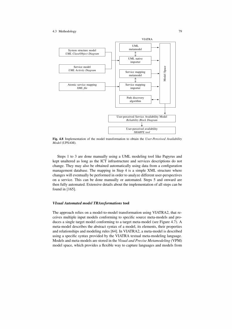
4.3 Methodology 79
UMLmetamodel
UML nativeimporter
Service mappingmetamodel
Service mappingimporter
Path discoveryalgorithm
Mod
elSp
ace
User-perceived Service Availability ModelReliability Block Diagram
User-perceived availabilitySHARPE tool
System structure modelUML Class/Object Diagram
Service modelUML Activity Diagram
Atomic service mappingXML file
VIATRA
Fig. 4.8 Implementation of the model transformation to obtain the User-Perceived AvailabilityModel (UPSAM).
Steps 1 to 3 are done manually using a UML modeling tool like Papyrus andkept unaltered as long as the ICT infrastructure and services descriptions do notchange. They may also be obtained automatically using data from a configurationmanagement database. The mapping in Step 4 is a simple XML structure wherechanges will eventually be performed in order to analyze different user-perspectiveson a service. This can be done manually or automated. Steps 5 and onward arethen fully automated. Extensive details about the implementation of all steps can befound in [165].
VIsual Automated model TRAnsformations tool
The approach relies on a model-to-model transformation using VIATRA2, that re-ceives multiple input models conforming to specific source meta-models and pro-duces a single target model conforming to a target meta-model (see Figure 4.7). Ameta-model describes the abstract syntax of a model, its elements, their propertiesand relationships and modeling rules [64]. In VIATRA2, a meta-model is describedusing a specific syntax provided by the VIATRA textual meta-modeling language.Models and meta-models are stored in the Visual and Precise Metamodeling (VPM)model space, which provides a flexible way to capture languages and models from

80 4 User-Perceived Service Availability
various domains by identifying their entities and relations. To import the UML mod-els into this model space, VIATRA2 provides a UML native importer and a UMLmeta-model. In order to import the service mapping pair into the model space, acustom service mapping meta-model and importer plug-in was developed based onthe hierarchy presented in Figure 4.5. The task of the services mapping importer isto parse the XML file, traverse the content tree and find appropriate VPM entitiesin the meta-model corresponding to the type of each element. It is implemented inthe Java programming language and added to the project workspace as an Eclipseplug-in. Additionally, the VIATRA2 textual command language provides a flexiblesyntax to access the VPM model space. It is based on mathematical formalismsand provides declarative model queries and manipulation [233]. This language isespecially useful in this methodology to implement the path discovery algorithm inSection 4.3.1.
4.3.1 Path Discovery Algorithm
As stated in Section 4.2.3, the service mapping pair gives the initial and final bound-aries of the ICT infrastructure used by a specific atomic service. In order to identifythe ICT components potentially required for service provision, all possible pathsbetween the service requester and provider must be traced. Multiple paths signif-icantly increase the availability of an atomic service, as they provide redundancy.This approach implies that topology changes on the ICT infrastructure do not re-quire adjustments to the service model or the atomic service mapping, given thatrequester and provider are still running on the same ICT components. For everyservice mapping pair, the algorithm discovers a set of paths between the respectiverequester and provider, and stores the visited entities in a reserved tree structureinside the model space.
The complexity of such algorithms grows significantly with the size of the ICTinfrastructure. In order to find all possible paths, every node must be visited throughall available edges. For this reason, the time complexity of the algorithm is evenmore sensitive to the number of edges, reaching O(n!) for a fully interconnectedgraph of n nodes. The complexity is a serious problem in networks with a highconnectivity, such as wireless mesh networks and the reason why the methodologyfor evaluation of service discovery responsiveness presented in Chapter 7 uses aprobabilistic path discovery. However, cabled networks usually contain few if anyloops, while most clients are located in tree-like structures with a low number ofedges. The path discovery algorithm used in this methodology was first describedin [2] and is based on the DFS algorithm [87], with a path tracking mechanismto avoid live-locks in cycles. It takes a pair of service requester and provider fromthe mapping model, identifies both in the graph representation of the network – ob-tained from the UML object diagram in Section 4.2.1 – and traces the paths betweenthem to be subsequently merged into a subgraph. This process is repeated for everyprovider described in the mapping model. This assures a precise solution at the cost

4.4 User-perceived Availability Model Generation 81
of a higher runtime, which proved to be acceptable for the case study networks inChapter 5. However, the methodology might as well use Probabilistic Breadth-FirstSearch (PBFS) as described in Section 7.3 to achieve better scalability.
4.3.2 User-perceived Service Infrastructure
The final step of the methodology is the generation of an output model by mergingthe paths obtained from the algorithm. Since all the atomic services within a givencomposite service are executed, their paths are also merged into one UML objectdiagram which corresponds to the partial infrastructure required for proper servicedelivery. The instance specifications of the UPSIM object diagram have the samesignature as in the original ICT infrastructure. Therefore, they maintain the sameset of properties as the classes they instantiate. It is thus guaranteed that a subse-quent service dependability analysis will find specific required properties for everyelement of the user-perceived ICT infrastructure. One such analysis could assessservice availability based on those properties, which is exactly what the UPSAMdoes. Details on the generation of the UPSAM can be found in Section 4.4.
4.4 User-perceived Availability Model Generation
Since all the atomic services within a given composite service may be executed, thepaths found in Section 4.3, Step 7 are merged into one model which corresponds tothe partial infrastructure required for proper service delivery of a given service pair.The UPSAM is a transformation of that partial infrastructure. The instance specifi-cations of the components within that partial infrastructure have the same signatureas in the original ICT infrastructure from Section 4.2.1. Therefore, they maintain thesame set of properties as the classes they instantiate. It is thus guaranteed that a sub-sequent availability analysis will find specific required properties for every elementof the UPSAM.
Each atomic service has its own set of paths. All ICT components forming thepath are translated into serialized blocks inside the RBD, given that all of themmust be working in order to traverse the path. If an ICT component has n redundantcomponents, the RBD will have n parallel blocks with the same characteristics. Thiscorresponds to the redundant components property of the profile (see Figure 4.2).An atomic service is available if all ICT components on at least one of its pathsare available. This introduces path redundancy inside the service network, and isrepresented within the RBD by placing blocks related to these paths in parallel.Identical blocks within those parallel paths are then merged into a single block.
Let us demonstrate this using Figure 4.9 as an example of an ICT infrastruc-ture model, ignoring the links for simplification purposes. The following paths areidentified from component A to G:

82 4 User-Perceived Service Availability
C
D E
F
G
BA
Fig. 4.9 ICT Infrastructure model example
A→ B→C→ D→ F → G
A→ B→C→ E→ F → G
Components A,B,C and F,G are represented as a series of blocks, as they arecommon for both paths. Blocks D and E are in series within their respective pathsbut parallel to each other. Thus, they are represented as a pair of parallel blocks inbetween the two sequences obtained previously. Given all components have no re-dundancy, only component B is triplexed (redundantComponents=2). Know-ing that B has two redundant components for a total of three components, it is rep-resented as three parallel blocks B. The resulting RBD is presented in Figure 4.10.Note that for steady-state evaluation, the order of the blocks does not affect the re-sulting availability. The individual RBDs of the atomic services are then connectedin a similar manner to an overall availability model of the composite service, ac-cording to the defined service model (see Section 4.2.2).
A
B
B
B
C
D
E
F G
Fig. 4.10 Reliability Block Diagram of the example ICT infrastructure model
Existing methodologies for steady-state availability analysis mostly use RBDsto represent their output models. If the focus of modeling is on failure instead ofsuccess conditions, FTs are used. Both models provide comparable analysis for dif-ferent points of view and are supported by the proposed methodology.
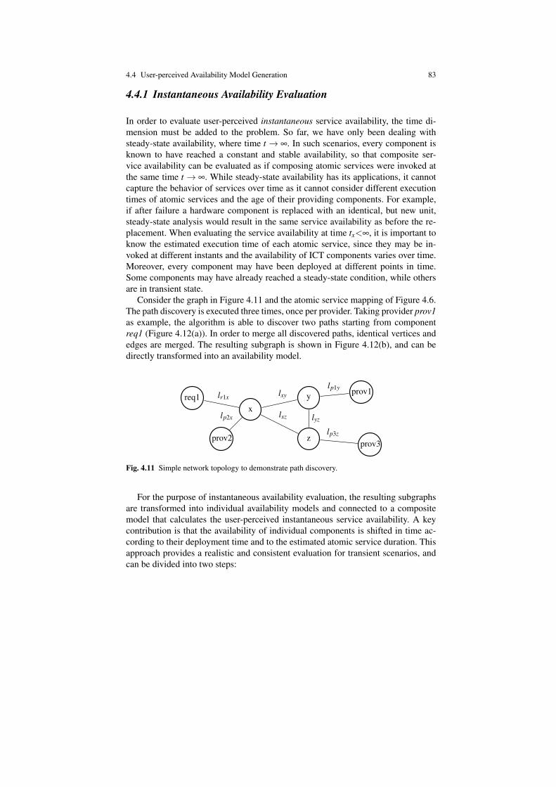
4.4 User-perceived Availability Model Generation 83
4.4.1 Instantaneous Availability Evaluation
In order to evaluate user-perceived instantaneous service availability, the time di-mension must be added to the problem. So far, we have only been dealing withsteady-state availability, where time t → ∞. In such scenarios, every component isknown to have reached a constant and stable availability, so that composite ser-vice availability can be evaluated as if composing atomic services were invoked atthe same time t → ∞. While steady-state availability has its applications, it cannotcapture the behavior of services over time as it cannot consider different executiontimes of atomic services and the age of their providing components. For example,if after failure a hardware component is replaced with an identical, but new unit,steady-state analysis would result in the same service availability as before the re-placement. When evaluating the service availability at time tx<∞, it is important toknow the estimated execution time of each atomic service, since they may be in-voked at different instants and the availability of ICT components varies over time.Moreover, every component may have been deployed at different points in time.Some components may have already reached a steady-state condition, while othersare in transient state.
Consider the graph in Figure 4.11 and the atomic service mapping of Figure 4.6.The path discovery is executed three times, once per provider. Taking provider prov1as example, the algorithm is able to discover two paths starting from componentreq1 (Figure 4.12(a)). In order to merge all discovered paths, identical vertices andedges are merged. The resulting subgraph is shown in Figure 4.12(b), and can bedirectly transformed into an availability model.
lr1x
lp2x
lxy
lxz lyz
lp1y
lp3z
req1
prov2
xy
z
prov1
prov3
Fig. 4.11 Simple network topology to demonstrate path discovery.
For the purpose of instantaneous availability evaluation, the resulting subgraphsare transformed into individual availability models and connected to a compositemodel that calculates the user-perceived instantaneous service availability. A keycontribution is that the availability of individual components is shifted in time ac-cording to their deployment time and to the estimated atomic service duration. Thisapproach provides a realistic and consistent evaluation for transient scenarios, andcan be divided into two steps:

84 4 User-Perceived Service Availability
(a)req1 lr1x x lxy y lp1y prov1
req1 lr1x x lxz z lzy y lp1y prov1
(b) req1 lr1x x y lp1y prov1lxy
lxz z lzy
Fig. 4.12 Paths between req1 and prov1 (a) and merged subgraph (b).
1. The Model generation step generates the service availability model, which iscomposed of the availability of individual components arranged according totheir roles in the service provision.
2. The Access time definition step complements the service availability model byidentifying the exact instant at which each component is invoked within its life-cycle.
The model generation for the atomic services is similar to the one described forsteady-state availability, while the access time definition warrants more detailed ex-planation in Section 4.4.2. The resulting user-perceived service availability model,represented in the FT in Figure 4.13, is composed of three main stages: (1) Com-posite service, (2) atomic services and (3) ICT components necessary for provisionof the atomic services.
C
B
A
S F
req1(ts,te)
req1prov1
123
lr1x(ts,te)
x(ts,te)
lxy(ts,te)
lxz(ts,te)
z(ts,te)
lzy(ts,te)
y(ts,te)
lp1y(ts,te)
prov1(ts,te)
D
Fig. 4.13 Partial fault-tree (FT) of the provided example.
We will now explain the three stages in detail using the example FT in Figure4.13. According to the service model in Figure 4.4, the condition for the compos-ite service S to fail is that at least one of the atomic services fails. Therefore, thefirst stage of this model can be represented in the rightmost part of the tree by asingle OR logic gate, where the number of input ports corresponds to the number

4.4 User-perceived Availability Model Generation 85
of atomic services. In stage two, every atomic service is represented by an ANDlogic gate with every provider connected to an input port. This logic gate representsthe condition that all providers must fail to result in an atomic service failure. Thisinformation is provided by the mapping model in Figure 4.6, which contains threeproviders prov1, prov2 and prov3. Stage three in Figure 4.13 does not have a fixedpattern. Its logical circuits depend exclusively on the subgraphs from Section 4.3.1.Components essential for service provision of a specific provider are connected toOR logic gates, while redundant components are connected to AND logic gates. Thethird stage shows the logic circuits of the resulting subgraph in Figure 4.12(b), cor-responding to communication between requester req1 and provider prov1 in Figure4.6.
The same problem can be modeled using an RBD, depicted in Figure 4.14. Thelayers 1, 2 and 3 correspond to the equivalent stages in Figure 4.13: Compositeservice S, atomic service C and component req1 using component prov1 when re-questing C. According to the RBD and FT formalisms, logical AND gates representparallel blocks while logical OR gates represent serial blocks. The models in Figures4.13 and 4.14, in addition to failure and repair rates of individual ICT components,are sufficient to evaluate the user-perceived steady-state service availability. In thenext section, the access time definition is explained that allows these models to eval-uate instantaneous availability of composite services.
atomic service C
2
composite service1
req1-prov1 of atomic service C
3
A B C D
req1-prov2
req1-prov1
req1-prov3
Areq1
(ts,te)Alr1x
(ts,te)Ax
(ts,te)Alxy
(ts,te)
Alxz
(ts,te)Az
(ts,te)Alzy
(ts,te)Ay
(ts,te)Alp1y
(ts,te)Aprov1
(ts,te)
Fig. 4.14 Partial reliability block diagram (RBD) of the provided example.

86 4 User-Perceived Service Availability
4.4.2 Access Time Definition
In a non-steady-state scenario, we want to evaluate how availability decreases overtime. The deployment time defines the instant at which individual components werefully available. Furthermore, using the additional information proposed in the map-ping model – duration and priority – it is possible to calculate when every singleatomic service provision is expected to start and finish. The assumption that everyservice provision starts at the same time is only valid for steady-state evaluation,where components have reached a stable availability – a proposition hardly realisticin dynamic and heterogeneous networks.
As seen in Section 4.4.1, the user-perceived service availability depends on theinterval availability of many components, according to their roles in their respectiveatomic services. Another option would be to use the instantaneous availability ofthose components at a specific instant within this interval. Picking the correct in-stant is not trivial, however. Using the start of the interval would lead to an overlyoptimistic estimation while using the end time might be too pessimistic, especiallyfor longer running atomic services. Picking any specific instant within the intervalwould need a sophisticated atomic service model with access durations for everycomponent and dependencies among them. It is unclear what such a model wouldlook like, knowing that components will change for every user-perspective, and howit could be reasonably validated to justify its usage. This is why this methodologyproposes to use interval availability, the average availability over the whole dura-tion of an atomic service. The exact range of the interval availability evaluation,however, is estimated according to the instant each component is invoked, taking itsdeployment time as reference. Initial references can be defined as follows:
• t0 of an individual component is independently defined as its owndeployment time.
• ta0 of a composite service is defined as t0 of the youngest component.
Furthermore, every atomic service is invoked at different instants, with ta0 asreference. Their initial times are set according to the service and mapping models,which denote the serial/parallel configuration of each atomic service, and providetheir estimated duration. As mentioned in Section 4.2.3, the estimated duration ofeach atomic service is given by the latest estimated end time minus the earliestestimated start time of its redundant providers.
As an example, consider the FT model in Figure 4.13. The relevant networkcomponents, required for the provision of atomic service C from provider prov1to requester req1, were deployed at different instants. In this example, componentsprov1 and lp1y are assumed the youngest and their deployment time is thereforetaken as reference time ta0. The composite service S will be invoked at t = ta0 +3600, that is, one hour after the youngest component was deployed. The atomicservice C, mapped in Figure 4.6, has an estimated duration of 18 seconds, as alreadydescribed in Section 4.2.3. Using similar analysis, the estimated duration of atomicservices A and B are set to 10 and 20. This way, it is possible to identify the timeintervals of each atomic service relative to the reference ta0:

4.4 User-perceived Availability Model Generation 87
tinvocation start,A = ta0 +3600 seconds
tinvocation end,A = ta0 +3600+10 seconds
tinvocation start,B = tinvocation start,A
tinvocation end,B = ta0 +3600+20 seconds
tinvocation start,C = tinvocation end,B
tinvocation end,C = ta0 +3600+38 seconds
The invocation start time of C is equal to the latest invocation end time of A andB, as it will be invoked only after both A and B have finished. The same applies toeach service provision within atomic services. Absolute start and end times of theavailability intervals of individual components i necessary for service provision pare given by:
ts,i = tinvocation start,p− tdeployment,i
te,i = tinvocation end,p− tdeployment,i
Let the deployment time of component x be ten days, hence, 864000 secondsbefore ta0. This way ts,x and te,x in the service provision req1-prov1 within atomicservice C are obtained as follows:
ts,x = ta0 +3600+20− (ta0−864000) = 867620te,x = ta0 +3600+38− (ta0−864000) = 867638
The interval unavailability Ux(ts, te) = 1− Ax(ts,x, te,x) for component x in theexample of Figure 4.13 should be calculated using Equation 4.1.
Ax(ts,x, te,x) =1
te,x− ts,x· te,x
ts,xAx(τ)dτ (4.1)
For constant failure and repair rates, Ax(τ) is given by Equation 2.5. A constantfailure rate is a reasonable approximation after the wear-in period of hardware com-ponents, in which faults become random and independent events along most of thecomponent lifetime. For the case study in Chapter 5, we will use this approxima-tion for all availability calculations. It should be mentioned that in scenarios wherethis approximation is not valid and non-constant failure rates are given, a differentinstantaneous availability equation could be derived using these non-constant ratesand used without further modifications within the proposed methodology.


Chapter 5Case Study of User-Perceived ServiceAvailability
Abstract This chapter demonstrates the feasibility of the methodology previouslyintroduced in Chapter 4 with a representative case study. We apply the methodologyto parts of the network infrastructure of University of Lugano (USI), Switzerland.This infrastructure consists of six interconnected routers and switches in its corewith servers directly connected to it, and tree-like peripheral networks composed ofclients and printers. First, a User-Perceived Service Infrastructure Model (UPSIM)is generated for two different clients of an exemplary mail service. User-perceivedsteady-state and instantaneous availability models are created for diverse scenar-ios. We show and discuss how availability changes in these scenarios and how themethodology enables assessment of these different results with very low effort.
5.1 Introduction
In this chapter, the feasibility of the methodology from Chapter 4 is demonstratedby generating the User-Perceived Service Infrastructure Model (UPSIM) and var-ious different User-Perceived Service Availability Models (UPSAMs) of an exem-plary Send mail service in a real network and from different user perspectives. Thetopology depicted in Figure 5.1 is based on the network of University of Lugano(USI), Switzerland. The network core, consisting of six interconnected routers andswitches in its core, is nearly identical to the real infrastructure while the tree-formedperipheral parts connected to the core, composed of clients and printers, have beenreduced for demonstration purposes. Servers are directly connected to the bottom-most switches. Every component has a unique ID and a specified type in the formatid : type. For better visualization, links lack labels. They are, however, referencedthroughout this chapter as the concatenated IDs of the devices they connect. Forinstance, the line between t1 and e1 represents a communication link identified byt1 e1. Links in this network are categorized either as wired or wireless, respectivelyrepresented by full or dashed lines. In Sections 5.2 and 5.3, only wired links aretaken into account.
89

90 5 Case Study User-Perceived Service Availability
D1:C3750D2:C3750
E1:HP2650 E4:HP2650
E2:HP2650 E3:HP2650
auth:Server :Server
email:Server :Server
T4:Comp
T3:Comp
T2:CompT1:Comp
T5:Comp
T6:Comp
T7:Comp
T8:Comp T10:Comp
T11:Comp
T12:Comp
T13:Comp
T14:Comp
T15:Comp
P2:Printer
P3:Printer
dns: Server:Server
T9:Comp
P1:Printer
C1:C6500 C2:C6500
D3:C2960 D4:C2960
backup file
file1
2 R
Fig. 5.1 Network infrastructure based on university campus network. Lines between devices rep-resent network links.
5.2 User-Perceived Service Infrastructure
A number of atomic services are provided in the network, such as Check authenti-cation, Dispatch email, Print document, Request backup and so forth, whereas each
service has at least one provider. Atomic services can compose composite services,
for example email, printing or backup, which are requested by different clients lo-
cated at various positions within the network. The following sections explicitly re-
flect the steps of the proposed methodology defined in Section 4.3.
5.2.1 Identification and Modeling of ICT Components
The ICT infrastructure is modeled with focus on service dependability assessment,
more specifically, steady-state and instantaneous availability. In order to use the

5.2 User-Perceived Service Infrastructure 91
UPSIM for user-perceived service availability assessment, we developed the sim-ple UML profile in Figure 4.2, which contains relevant properties for such analysis.This profile is then applied to the infrastructure. Each ICT component, device orconnector, has intrinsic dependability attributes such as a failure rate, a repair rateand a number of internal redundant components. In this case study, we assume thatthese rates are constant, and that the failure rate encapsulates all possible failurecauses within the scope of a component, e.g. hardware or software. As mentioned inSection 4.4.2, this assumption does not necessarily hold. In scenarios where func-tions of non-constant rates are given, a different equation to calculate instantaneousavailability of individual components could be derived and used without furthermodifications within the proposed methodology.
As can be seen in the availability profile in Figure 4.2, although Device and Con-nector inherit the same attributes from Component, they are distinguished in orderto be applied – respectively and exclusively – to Class and Association elements.
The different types of ICT components identified in the infrastructure model(Figure 5.1) are modeled in a set of stereotyped classes depicted in Figure 5.2,which shows the UML class diagram containing the description of the devices andtheir connections as, respectively, classes and associations. This diagram containsall network elements with their predefined availability properties. At this point, weevaluate all constituting devices and their possible connections. For instance, D1and D2 are different instances of the same device labeled C3750, which is knownto be a switch. Therefore, the corresponding class is created, with Component andSwitch stereotypes applied from the availability and network profiles. When all de-vices are represented as classes, their possible links are represented by associationsstereotyped as Component and Communication.
As another example for the ICT component description in UML, in Figure 5.2the type RServer represents a server containing an internal redundancy of oneextra component (redundantComponents=1) which signifies that there are ac-tually two servers with one server to fail over. Type C2960 represents a switch. Thecomplete list of ICT components including relevant availability data is presented inTable 5.1.
5.2.2 ICT Infrastructure Modeling
The infrastructure object diagram (see Figure 5.3) is built with instances of classesand associations (namely instanceSpecification and links) from the previous step,and reflects the topology of the network in Figure 5.1. Since attributes are staticallydefined in classes, those instances are already well-defined components. Also, giventhat links are instances of associations, connections are possible only when thoseassociations exist.
In the UML object diagram in Figure 5.3, each node is represented by a uniqueidentification and the respective type, in the format id:Type. Types HP2650,C3750, C6500 and C2960 are switches, the other types should be self-explanatory.

92 5 Case Study User-Perceived Service Availability
<<component;server>>Server
<<Component >>
failureRate: 1,67 ·10−5
repairRate: 10redundantComponents: 0
<<Server >>
<<component;switch>>C2960
<<Component >>
failureRate: 5,45 ·10−6
repairRate: 2redundantComponents: 0
<<Switch >>
<<component;switch>>C6500
<<Component >>
failureRate: 1,63 ·10−5
repairRate: 2redundantComponents: 0
<<Switch >>
<<component;rserver>>RServer
<<Component >>
failureRate: 1,67 ·10−5
repairRate: 10redundantComponents: 1
<<RServer >>
<<component;switch>>HP2650
<<Component >>
failureRate: 5,025 ·10−6
repairRate: 2redundantComponents: 0
<<Switch >>
<<component;switch>>C3750
<<Component >>
failureRate: 5,303 ·10−6
repairRate: 2redundantComponents: 0
<<Switch >>
<<component;client>>Comp
<<Component >>failureRate: 0,00033repairRate: 0,04167redundantComponents: 0
<<Client >>
<<component;printer>>Printer
<<Component >>failureRate: 0,00035repairRate: 1redundantComponents: 0
<<Printer >>
<<communication;connector>>
Fig. 5.2 Predefined network elements classes.
Table 5.1 Specification of ICT components
Type Manufacturer Model Failure rate (1/h) Repair rate (1/h) RC*
C2960 Cisco Catalyst 2960-48FPD-L 5,45 ·10−6 2 0C6500 Cisco Catalyst 6500 1,63 ·10−5 2 0C3750 Cisco Catalyst 3750G-24TS 5,303 ·10−6 2 0HP2650 Hewlett-Packard ProCurve 2650 5,025 ·10−6 2 0Server Dell PowerEdge T620 1,67 ·10−5 10 0RServer Dell PowerEdge T620 1,67 ·10−5 10 1Comp HP Compaq DC7800 0,000333 0,04167 0Printer Canon IR3245N 0,001389 2 0Wired link n/a n/a 7,69 ·10−6 0,25 0Wireless link n/a n/a 0,0833 33,333 0*redundantComponents

5.2 User-Perceived Service Infrastructure 93
t6:Compt6:Comp
t7:Compt7:Comp
t8:Compt8:Comp
t10:Compt10:Comp
t11:Compt11:Comp
t12:Compt12:Comp
t5:Compt5:Comp
e2:HP2650e2:HP2650
e3:HP2650e3:HP2650
p2:Printerp2:Printer
t4:Compt4:Comp
t9:Compt9:Comp
p1:Printerp1:Printer
t13:Compt13:Comp
t3:Compt3:Comp
e1:HP2650e1:HP2650
d1:C3750d1:C3750
d2:C3750d2:C3750
e4:HP2650e4:HP2650
t14:Compt14:Comp
t2:Compt2:Comp
t1:Compt1:Comp
c1:C6500c1:C6500
c2:C6500c2:C6500
p3:Printerp3:Printer
t15:Compt15:Comp
auth:Serverauth:Server
d3:C2960d3:C2960
d4:C2960d4:C2960
file1:Serverfile1:Server
backup:Serverbackup:Server
email:Serveremail:Server
file2:Serverfile2:Server
dns:RServerdns:RServer
Fig. 5.3 Network infrastructure presented in UML Object Diagram
Given that RServer has redundantComponents = 1, the dns is then known to haveredundancy although represented by a single node.
5.2.3 Identifcation and Modeling of Services
The exemplary Send mail service of this case study consists of resolving the MailExchanger (MX) address via the Domain Name System (DNS) and then sendingan email message over that MX by means of the common Simple Mail TransferProtocol (SMTP). During SMTP communication, the MX checks the credentialsprovided by the client with an external authentication server. This service representsa widespread use-case in present-day service networks. In detail, the service is com-posed of three atomic services, used in sequential order. Following is a descriptionof the atomic services:
1. Resolve mail server address – A client first uses the DNS to resolve the MXrecord, an IP address of the mail server.
2. Dispatch email via SMTP – The client connects to the MX using that address. Itwill then send an email message over that MX by means of the common SMTP.
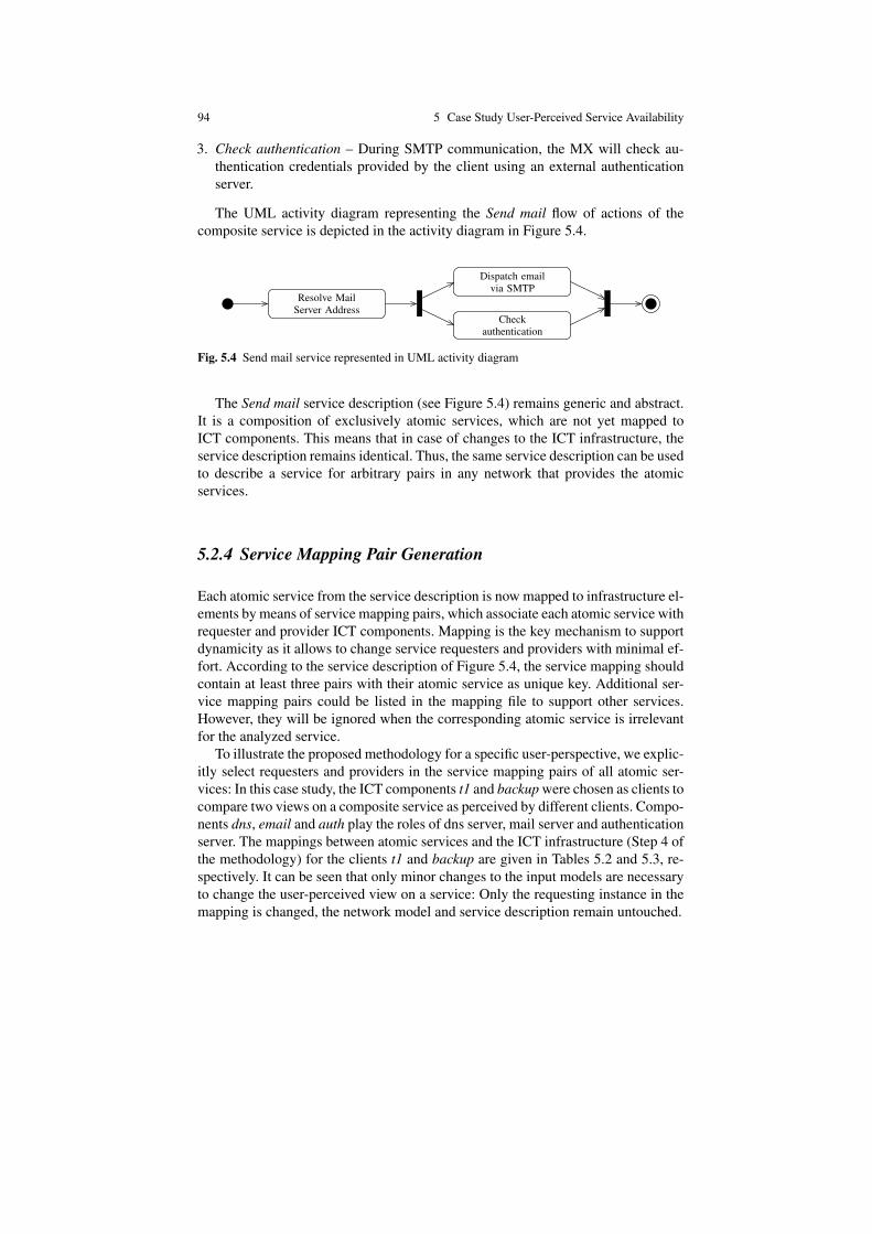
94 5 Case Study User-Perceived Service Availability
3. Check authentication – During SMTP communication, the MX will check au-thentication credentials provided by the client using an external authenticationserver.
The UML activity diagram representing the Send mail flow of actions of thecomposite service is depicted in the activity diagram in Figure 5.4.
Resolve MailServer Address
Dispatch emailvia SMTP
Checkauthentication
Fig. 5.4 Send mail service represented in UML activity diagram
The Send mail service description (see Figure 5.4) remains generic and abstract.It is a composition of exclusively atomic services, which are not yet mapped toICT components. This means that in case of changes to the ICT infrastructure, theservice description remains identical. Thus, the same service description can be usedto describe a service for arbitrary pairs in any network that provides the atomicservices.
5.2.4 Service Mapping Pair Generation
Each atomic service from the service description is now mapped to infrastructure el-ements by means of service mapping pairs, which associate each atomic service withrequester and provider ICT components. Mapping is the key mechanism to supportdynamicity as it allows to change service requesters and providers with minimal ef-fort. According to the service description of Figure 5.4, the service mapping shouldcontain at least three pairs with their atomic service as unique key. Additional ser-vice mapping pairs could be listed in the mapping file to support other services.However, they will be ignored when the corresponding atomic service is irrelevantfor the analyzed service.
To illustrate the proposed methodology for a specific user-perspective, we explic-itly select requesters and providers in the service mapping pairs of all atomic ser-vices: In this case study, the ICT components t1 and backup were chosen as clients tocompare two views on a composite service as perceived by different clients. Compo-nents dns, email and auth play the roles of dns server, mail server and authenticationserver. The mappings between atomic services and the ICT infrastructure (Step 4 ofthe methodology) for the clients t1 and backup are given in Tables 5.2 and 5.3, re-spectively. It can be seen that only minor changes to the input models are necessaryto change the user-perceived view on a service: Only the requesting instance in themapping is changed, the network model and service description remain untouched.

5.2 User-Perceived Service Infrastructure 95
Table 5.2 Service mapping pairs of the Send mail service for client t1.
Atomic Service Requester Provider
Resolve mail server address t1 dnsDispatch email via SMTP t1 emailCheck authentication email auth
Table 5.3 Service mapping pairs of the Send mail service for client backup.
Atomic Service Requester Provider
Resolve mail server address backup dnsDispatch email via SMTP backup emailCheck authentication email auth
5.2.5 Model Space Import
Next, we are running the VIATRA2 native UML2.2 importer on all files contain-ing the set of input diagrams (profiles, class diagram, object diagram and activitydiagram). As described in Section 4.3, the import of the service mapping pairs tothe VIATRA2 model space is accomplished with a custom-developed service map-ping metamodel and importer plug-in. The XML file is parsed and the content treetraversed to identify elements. All import steps are completely automated.
5.2.6 Path Discovery for Service Mapping Pairs
In this step, the elements of each service mapping pair are matched to ICT compo-nents of the infrastructure (see Figure 5.1). The algorithm sees the infrastructure asa graph and iteratively extracts all possible paths between two vertices requester andprovider. For instance, for the first service mapping pair of Table 5.2, the discoveryfor client t1 identifies eight acyclic ways to reach dns:
t1→ e1→ d1→ c1→ c2→ d4→ dns
t1→ e1→ d1→ c1→ c2→ d4→ dns
t1→ e1→ d1→ c1→ d2→ c2→ d4→ dns
t1→ e1→ d1→ c1→ d3→ c2→ d4→ dns
t1→ e1→ d1→ c2→ d4→ dns
t1→ e1→ d1→ c2→ c1→ d4→ dns
t1→ e1→ d1→ c2→ d2→ c1→ d4→ dns
t1→ e1→ d1→ c2→ d3→ c1→ d4→ dns

96 5 Case Study User-Perceived Service Availability
These paths are then added to the VIATRA2 model space for further manipula-tion. The path discovery algorithm has been implemented using the VTCL languageprovided by VIATRA2. This step is completely automated.
5.2.7 User-Perceived Infrastructure Model Generation
The final step comprises of matching the elements of the paths obtained in the pre-vious step (Section 5.2.6) to the complete infrastructure given by the second step(Section 5.2.2). This step is fully automated and behaves like a filter on the com-plete topology, where only nodes which appear at least once in the discovered pathsare preserved. Multiple occurrences are ignored. The output model is a UML objectdiagram containing only that fragment of the infrastructure required for the execu-tion of the Send mail service from client t1, all redundant paths taken into account.This user-perceived service infrastructure model is shown in Figure 5.5a. The typesof InstanceSpecifications are adopted from the input infrastructure object diagram.Therefore, the service and network properties (failure rate, repair rate, etc.) are au-tomatically inherited from the instantiated classes. Services and dependability prop-erties are now correlated, facilitating extraction for further analysis. To generate theUPSIM for the second perspective, the Send mail service from client backup usingthe same atomic service providers, we only have to make minor adjustments to theservice mapping. Figure 5.5b shows the UPSIM from this user perspective.
The generated UPSIM can be used to visualize the set of ICT components andtheir connections relevant for a particular pair requester and provider. This alone isvery helpful in case of service problems, as it provides a quick overview on whichICT components might be the cause. More important, the UPSIM can be used to fa-cilitate analysis of various user-perceived dependability properties (e.g.: availability,performability, responsiveness). For example, it can be used to assess user-perceivedsteady-state availability for a service, that is, the ratio of operational time over thelivetime of a service, observed by a particular user. Such analysis can be performedby transforming the UPSIM to a RBD or FT, in which entities correspond to com-ponents of the UPSIM. The availability for individual components can be calculatedusing the component attributes failure rate and repair rate, as seen in Formula 2.10.The service availability can then be computed using the RBD or FT. We presentthis complementary transformation to RBDs in Section 5.3. More details about theprocess can be found in [5].
5.3 User-Perceived Steady-State Availability
We will now demonstrate the evaluation of user-perceived availability using themethodology from Section 4.4 with the exemplary Send mail service. We simplifythe fault model by taking only the steady-state availability of ICT components into

5.3 User-Perceived Steady-State Availability 97
e1:HP2650e1:HP2650
d1:C3750d1:C3750
d2:C3750d2:C3750
t1:Compt1:Comp
c1:C6500c1:C6500
c2:C6500c2:C6500
auth:Serverauth:Server
d3:C2960d3:C2960
d4:C2960d4:C2960
email:Serveremail:Server
dns:RServerdns:RServer
(a) Requested by client t1.
d1:C3750d1:C3750
d2:C3750d2:C3750
c1:C6500c1:C6500
c2:C6500c2:C6500
auth:Serverauth:Server
d3:C2960d3:C2960
d4:C2960d4:C2960
backup:Serverbackup:Server
email:Serveremail:Server
dns:RServerdns:RServer
(b) Requested by client backup.
Fig. 5.5 UPSIM of Send mail service for two different user perspectives.
account. This means we assume that all faults from classes fail stop to byzantineare combined in the steady-state availability of the individual ICT components. Anordered fault classification can be found in [25]. We also disregard service discov-ery: The DNS server address is known a priori to the client as is the authenticationserver address to the MX. In the following, we will generate the UPSAM for thefirst atomic service of the Send mail service, Resolve mail server address. Genera-tion for the subsequent atomic services is omitted but will adhere to the exact sameprocedure.
As described in Section 4.3, the ICT infrastructure is represented by a UMLobject diagram, where each node is an instance of a specific ICT component classdescribed in a UML class diagram. The links between nodes are also representedas instances of associations from the UML class diagram. For simplification, in this

98 5 Case Study User-Perceived Service Availability
specific evaluation associations are given the maximum availability of 1 – meaningthat they are always available – for the sole purpose that their respective RBD blockscan be omitted in illustrations without affecting the steady-state availability. The fulltopology object diagram is shown Figure 5.3.
For UPSAM generation, instead of generating the UPSIM as described in Section5.2.7, the paths discovered in the step described in Section 5.2.6 are merged andtransformed into a single RBD. For requester t1, this RBD is shown in the upper partof Figure 5.6. This procedure basically corresponds to Step 9a of the methodologydetailed in Section 4.3. It reduces common nodes of different paths and excludesthose which do not affect the overall availability of the service. For instance, in orderto pass through d2, nodes c1 and c2 must be available, in addition to the commonnodes t1, e1, d1, d4 and dns. However, their availability implies that there is alreadyat least one path guaranteed to be available between d1 and d4. This is becauseassociations have an availability of 1 and there are associations between c1 andd1,d4 as well as between c2 and d1,d4. For this reason, the node d2 does not affectthe overall steady-state availability and is excluded from the UPSAM. Furthermore,redundant components are expanded: The dns component is converted into a pair ofparallel blocks dns1 and dns2.
t1 e1 d1
c1
c2
d4
dns1
dns2
backup d3
c1
c2
d4
dns1
dns2
Fig. 5.6 User-perceived service availablity models (UPSAM) of atomic service Resolve mailserver address for requesters t1 and backup.
Figure 5.6 shows the UPSAM for requester t1 side by side with the analogouslycreated UPSAM for requester backup. We see only minor differences in the twomodels because to reach dns, both requesters have to use almost the same part of thenetwork. Both have to traverse the network core, only the entry points are different.The next atomic service Dispatch email via SMTP paints a different picture. Toreach the mail exchanger, requester backup does not need to traverse the networkcore, drastically reducing the number of blocks in the reliability block diagram. TheUPSAMs for these user perspectives are depicted in Figure 5.7.
Next, a composite UPSAM is created from the atomic UPSAMs according to theservice description in Figure 5.4. Although the Send mail service described in theactivity diagram contains a parallel execution, every single atomic service must beconcluded in order to accomplish the execution of the composite service. For thisreason, the resulting UPSAMs of the individual atomic services are put in series to

5.3 User-Perceived Steady-State Availability 99
t1 e1 d1
c1
c2
d3 email
backup d3 email
Fig. 5.7 User-perceived service availablity models (UPSAM) of atomic service Dispatch emailvia SMTP for requesters t1 and backup.
compose the overall UPSAM of the composite service Send mail, as presented inFigure 5.8. This corresponds to Step 9b of the methodology detailed in Section 4.3.For the sake of clarity, the atomic service RBDs have been combined into singleblocks in the figure.
Resolve mailserver address
Dispatch emailvia SMTP
Checkauthentication
Fig. 5.8 Service availablity model of the Send mail service
As the last step, we use the SHARPE tool [224] to solve the obtained UPSAM tocalculate the steady-state availability for the composite service Send mail. Resultsare shown in Table 5.4. We included results for the same service as requested byclient backup to show how two different user perspectives on the same service differin their availability.
Table 5.4 Service availability of Send mail service from different user perspectives
Service Requester t1 Requester backup
Resolve mail server address (atomic) 0.999912118 0.999992884Dispatch email via SMTP (atomic) 0.999910452 0.999993942Check authentication (atomic) 0.999993942 0.999993942
Send mail (composite) 0.999816521 0.999980768
In fact, altough the availability is reasonably high for both clients, it is an orderof magnitude higher when the same service is requested by client backup insteadof client t1 (1.6 hours downtime per year for client t1 versus 10 minutes for clientbackup). This justifies the approach of considering user-peceived service availabil-ity. These differences are expected to be of a much higher magnitude in more het-erogeneous networks with a significant variability in availability of the various com-ponent types, especially when taking into account different link qualities. In Section5.4, we introduce several types of heterogeneity, such as varying link quality and
100 5 Case Study User-Perceived Service Availability
component age to provide a more complete picture of user-perceived service avail-ability.
5.4 User-Perceived Instantaneous Availability
This section demonstrates the proposed methodology for instantaneous availabilityevaluation applied to the previously described illustrative Send email service. Threeatomic services compose the service, as depicted in Figure 5.4. This part of the casestudy slightly modifies server positions from Figure 5.1 and introduces a wirelesslink. These changes are introduced solely to exemplify conceptual differences ofthe types of analysis. For example, network links now have a realistic availability tointegrate varying link quality into the analysis. We also include external redundancyrepresented by redundant providers of an atomic service at different positions inthe network, as opposed to internal redundancy in previous sections, which meansidentical redundant providers at the same position in the network. This also leads toa UML object diagram updated from Figure 5.3.
Failure and repair rates are again set according to their types as in Table 5.1. Butto allow instantaneous availability assessment, the deployment times are providedindividually for each component in Table 5.5. Times are represented in epoch time,where 0 denotes midnight on the 1st of January, 1970. For each link, this correspondsto the time of deployment of the youngest component connected to its edges. Forinstance, link c1 d3 was deployed on epoch time 1366027200, which is the sameas for d3 and later than 1346511000 for c1. Reasonable values that could reflect areal world example were chosen for all components. In an actual network infras-tructure, both tables could be updated at run-time using monitoring information anda configuration management database.
Two distinct scenarios will now be evaluated. First, the variance of instantaneousavailability from different user perspectives is demonstrated in Section 5.4.1). Theimpact of changing the age or number of components is investigated in Section5.4.2. The resulting RBDs and FTs are too complex to be visually presented in areasonable manner in this section and are thus left out. Only the results of theirevaluation are shown instead.
5.4.1 Different User Perspectives
In this scenario, three different clients t1, t2 and printer p2 are requesting Send email.As can be seen in Figure 5.9, component t1 is connected to e1 via a wired link.The mapping model of this scenario is shown in Table 5.6. As opposed to t1, t2 isconnected to e1 via a wireless link. The rest of the infrastructure remains unchanged,so the only difference from client t1 is a less reliable link. The third client, printerp2, connects to the network from a completely different position. The change of user

5.4 User-Perceived Instantaneous Availability 101
D1:C3750
D2:C3750
E1:HP2650E4:HP2650
E2:HP2650 E3:HP2650
auth:Server backup:Server
email:Server db:Server
T4:Comp
T3:Comp
T2:CompT1:Comp
T5:Comp
T6:Comp
T7:Comp
T8:Comp T10:Comp
T11:Comp
T12:Comp
T13:Comp
T14:Comp
T15:Comp
P2:Printer
P3:Printer
dns1:Serverdns2:Server
T9:Comp
P1:Printer
C1:C6500 C2:C6500
D3:C2960 D4:C2960
Fig. 5.9 Network infrastructure based on university campus network, slightly modified server po-sitions for case study. Lines between devices represent network links, a dashed line constitutes awireless link.
perspective for t2 and p2 is achieved with only minor modifications to the mappingmodel, changing the requester component of the atomic services Resolve addressand Dispatch email in Table 5.6. The methodology then automatically generatesdifferent availability models.
The reference time t0 of this evaluation corresponds to the deployment time of thenewest component potentially required during service provision, component auth atepoch time 1366108200 for all three clients. Instantaneous availability A(t) is thencalculated over t until it reaches a steady-state condition. Although this networkcontains younger components, these were not identified by the path discovery aspotentially required during service provision and have no impact on this analysis.The resulting diagram for the instantaneous availability of Send email when invokedat time t is presented in Figure 5.10. Send email is not fully available at t0 becausenot all components were deployed at that exact time. This means that while somecomponents may have reached a steady-state condition, others will be in a transient

102 5 Case Study User-Perceived Service Availability
Table 5.5 Deployment times of individual ICT components.
ID Deployment time (s) ID Deployment time (s)
t1 1366043100 e3 1366016400t2 1366024200 e4 1367073300t3 1368788400 d1 1366038000t4 1368896400 d2 1346511000t5 1366013700 d3 1366027200t6 1366459200 d4 1346511000t7 1366545600 c1 1346511000t8 1367778000 c2 1346511000t9 1369040400 p1 1366027200t10 1366016400 p2 1366099200t11 1366026600 p3 1368361800t12 1366026600 backup 1368446400t13 1367073300 db 1365850800t14 1367073900 dns2 1366027200t15 1367247600 auth 1366108200e1 1366038000 email 1366050000e2 1366013700 dns1 1355572800
Table 5.6 Mapping model of client t1 for Send email. For other clients simply all occurences of t1have to be changed to the new client.
Atomic Service Requester Timeout Provider Prio Durat.
Resolve address t1 10s dns1 0 2 secdns2 1 2 sec
Dispatch email t1 10s email 0 5 secCheck auth. email 2s auth 0 2 sec
state. Over time, the availability decreases until also the most recently deployedcomponents, in this case auth and d3 auth, reach their individual steady-state avail-ability. Figure 5.10 shows a comparison of the instantaneous availability of Sendemail when invoked by clients t1 (dotted line), t2 (full line) and p2 (dashed line).Some corner values are shown in Table 5.7 with the instantaneous availability A(ta0)at the reference time, the steady-state availability A and difference of the two.
Table 5.7 Availability numbers of Send email service for different user perspectives.
Requester A(ta0) A A(ta0)−A
t1 0.9955 0.9916 0.0039 → 5.616 min/dayt2 0.9922 0.9891 0.0031 → 4.464 min/dayp2 0.9990 0.9989 0.0001 → 0.175 min/day
The steady-state availability for t1 is 0.9916 and that of t2 is 0.9891. This trans-lates to 3 days of downtime per year for Send email when requested by t1 versus

5.4 User-Perceived Instantaneous Availability 103
0.988
0.990
0.992
0.994
0.996
0.998
1.000
Time t
A(t)
ta0 +1 week +2 weeks
t1
t2
p2
Fig. 5.10 Instantaneous availability over time of Send email service for three different clients.
almost 4 days when requested by t2. In both scenarios, the links between clientst1 and t2 and the device e1 have a time redundancy when the DNS service is re-quested. If the first request to dns1 fails, the links will be tried again by requestingdns2. So with respect to t1 e1 and t2 e1, the DNS service will be successful whenthey are available either during the first or the second request. This can be modeledas a system of parallel availability blocks. During a subsequent request to the emailserver, the links are again accessed, which can be modeled as a block in series to theprevious parallel system.
The evaluation of links t1 e1 and t2 e1 according to their access order in thissystem of two parallel blocks in series with a single block, results in the steady-stateavailability of 0.99997 and 0.9975, corresponding to the one for wired and wirelesslinks, respectively. The ratio of these values resembles the ratio of the compositeservice steady-state availabilities for t1 and t2, since the only difference betweenthem is the link from the clients to e1. A(t) of p2 is much higher than the one oft1 and t2. It is also notably more stable: While the difference between A(ta0) andA is minor for the printer, it sums up to a few minutes per day for the two clientcomputers, as can be deducted from Table 5.7. The scenario shows that the proposedmethodology is able to capture diverse availabilities of the same service, dependingon which client is using it and also, that the variation of availabilities is differentover time.
5.4.2 Adding and Replacing Equipment
The second scenario evaluates how A(t) changes when a set of network componentsis added or replaced. Evaluation is again done from the perspective of t1 with refer-ence time ta0. This time, dns2 is absent during the first week. In the mapping model,this fact is reflected by having no redundant provider for the first atomic service.

104 5 Case Study User-Perceived Service Availability
The next event is a renewal of equipment in the lab room where components t1, t2,t3, t4 and e1 were located (see Figure 5.9).
In Figure 5.11, the availability with a single DNS server reaches a lower steady-state availability of 0.984 during the first week, against 0.9916 with redundant DNSproviders. The addition of dns2 after one week increases the availability of the com-posite service considerably. However, adding dns2 alone does not show a signif-icant effect on instantaneous availability, as all but one component necessary toreach dns2, link dns2 d3, are also required to access components dns1 and email.All of the are already close to a steady-state condition. Thus, A(t) for Send emaildecreases only minimally over a few days to steady-state availability before the labroom equipment is exchanged. Following the replacement, A(t) reaches 0.9997 asnew components are known to be fully available. The individual component avail-ability then decreases until they again reach a steady-state condition, bringing theoverall service availability to the same level as before. Results are summed up inTable 5.8, steady-state values for A represent the lowest values within the evaluatedperiod.
Page 1
0.9820.9840.9860.9880.9900.9920.9940.9960.9981.000
Time t
A(t)
ta0 +1 week +2 weeks
t1
Fig. 5.11 Instantaneous availability over time of Send email service for client t1 when changingequipment.
Table 5.8 Availability of Send email for t1 when changing components.
Requester A(ta0) A A(ta0)−A
only dns1 0.991091 0.983619 0.007472 → 10.76 min/daydns1, dns2 0.991609 0.991605 0.000004 → 0.3 sec/daynew lab 0.999674 0.991612 0.008063 → 11.61 min/day
When exactly the availability of a service will reach steady-state depends onthe individual characteristics of the deployed components. Usually, the instanta-neous availability will tend to steady-state availability after a duration in the order

5.5 Conclusion 105
of few weeks without changes in the network. In a regular network with a reason-able amount of components and dynamics, it is very rare to have weeks without anychanges to the ICT infrastructure. This means that at any time, there will be at leastsome user-perspectives in a transient state, which justifies the decision to evaluateinstantaneous availability.
5.5 Conclusion
The evaluation of availability over time concludes this part about user-perceived ser-vice availability evaluation. Dependability assessment in modern service networksremains challenging. It has been demonstrated that service availability indeed de-pends considerably on the properties of the providing ICT infrastructure. This isexpected to be true for dependability properties other than availability as well. Themethodology presented in Chapter 4 facilitates the automated calculation of suchuser-perceived properties. The separation of input models allows for quick updatesin dynamic networks. However, parts of the methodology have limits regarding theirscalability. Future research should focus on reducing the complexity of those parts.For example, we will show in Chapter 7, how in specific networks the exact pathdiscovery may be replaced by a stochastic method.
The presented service models still do not include the Service Discovery (SD)process. It could be included as a first service in series with the original service de-scription. The duration of this SD service would be the deadline until SD is requiredto have successfully enumerated all providers of subsequent services in the servicemodel. The availability of this SD service thus reflects the probability of SD to fin-ish successfully until the deadline, or in other words, its responsiveness. Part III ofthis work covers the metric SD responsiveness and the models presented in Chapter7 allow to calculate it.


Part IIIService Discovery Responsiveness

In service networks, Service Discovery (SD) plays a crucial role as a layer whereproviders can be published and enumerated. This part focuses on the responsivenessof the discovery layer, the probability to operate successfully within a deadline, evenin the presence of faults.
We approach SD responsiveness by evaluating it in two different experiment en-vironments in Chapter 6. Both setups evaluate common protocol implementations toprovide a realistic view on the responsiveness of active SD. First, a virtual testbed isset up with a simplified communication fault model that includes only packet loss.This is done to isolate the impact of packet loss on responsiveness as it is expectedto have a major influence. Next, similar experiments are run using the previouslyintroduced experiment framework ExCovery on the Distributed Embedded Systems(DES) testbed at Freie Universitat Berlin. In the DES testbed, instead of injectingfaults, varying load conditions provoke realistic fault behavior.
Following the experiments, a hierarchy of stochastic models for decentralized SDis proposed in Chapter 7. It is used to describe the active discovery of a single ser-vice using three popular SD protocols. A methodology to use the model hierarchyin wireless mesh networks is introduced. Given a pair requester and provider, a dis-covery protocol and a deadline, it generates specific model instances and calculatesresponsiveness. This process is supported by the Monte Carlo method Probabilis-tic Breadth-First Search (PBFS), which estimates various metrics for the propaga-tion of discovery packets. Furthermore, a new metric Expected Responsiveness Dis-tance der is introduced, to estimate the maximum distance from a provider whererequesters can still discover it with a required responsiveness. Using monitoringdata from the DES testbed, it is shown how responsiveness and der of the protocolschange depending on the position of nodes and the link qualities in the network.Chapter 8 uses data from experiments to validate the developed models. Two waysof solving the models are evaluated. First, the full model hierarchy is solved basedon low level monitoring data from the routing layer. Second, only the applicationlevel discovery model is solved using a history of SD communication measure-ments. Results show that the discovery model estimations correlate almost perfectlywith the real responsiveness. In the absence of SD communication measurements,the full model hierarchy provides reasonable estimations given that the low levelmonitoring data is accurate.
Both the extensive series of experiments and the analytical model results givevaluable insight into the responsiveness of SD that can help to improve future re-search on the dependability of service usage as a whole.

Chapter 6Experimental Evaluation of DiscoveryResponsiveness
Abstract As a time-critical operation, an important metric of Service Discovery(SD) is responsiveness – the probability of successful discovery within a deadline,even in the presence of faults. To get an idea about the responsiveness of SD inrealistic scenarios, this chapter provides an evaluation from a comprehensive set ofexperiment series. We present results of the evaluation of decentralized SD, specif-ically active SD using Zeroconf . To identify the main impairments to SD respon-siveness, two different experiment setups are chosen. First, we examine SD respon-siveness under the influence of packet loss in a controlled virtual platform. We showthat responsiveness decreases significantly already with moderate packet loss andbecomes practicably unacceptable with higher packet loss. Second, we examine SDin the Distributed Embedded Systems (DES) wireless testbed at Freie UniversitatBerlin. We demonstrate how the responsiveness changes depending on the distanceof actors and the load on the network. The experiments reveal packet loss, packetdelay and the position of SD actors as main factors influencing SD responsiveness.The results clearly demonstrate that in all but the most favorable conditions, theconfigurations of current SD protocols struggle to achieve a high responsiveness.We further discuss results that reflect the long-term behavior of the wireless testbedand how its varying reliability may impact SD responsiveness.
6.1 Introduction
Rather than developing an analytical model, which will be presented in Chapter 7,this chapter approaches the responsiveness of Service Discovery (SD) in a series ofexperiments. The experiments serve the following purposes:
1. To provide a general overview on SD responsiveness using a virtual experimentenvironment with a simplified fault model. For several realistic discovery scenar-ios, the responsiveness of active SD using Zeroconf [55] is shown depending on
109

110 6 Experimental Responsiveness Evaluation
the deadline tD of the discovery operation, the packet loss rate and the requirednumber p of providers P to be discovered.
2. To allow a deep insight into SD responsiveness in WMNs, similar scenarios areexamined in experiments carried out in the Distributed Embedded Systems (DES)wireless testbed at Freie Universitat Berlin. Responsiveness is evaluated depend-ing on the distance of actor nodes and the load in the network. This analysisis done both for the individual SDP packets as well as the complete discoveryoperation, which includes retries by the requester in case response packets donot arrive in time. The former allows to infer conclusions for other applicationprotocols which use similar packets and can provide input for analytical modelspresented in Chapter 7. As such, the gained results could be used to verify thevalidity of employing these models when optimizing the responsiveness of SDconfigurations in WMNs.
3. To demonstrate how to use ExCovery for experiments in the wireless DES testbedand how the comprehensive range of measurements stored during runs facilitatesdiverse types of analyses.
4. To show the long-term behavior of the DES testbed and demonstrate the effectsof internal and external faults. These faults are being recorded by ExCovery dur-ing experiment execution and have to be taken into account when interpreting theresults. Internal faults contain node crashes or clock drifts, external faults com-prise all types of wireless interference or forced interruptions during executionof experiments.
The focus of the evaluation is on active SD (see Section 2.2.2), where a clientactively sends out discovery requests, retrying in case not enough valid responseswere received until a timeout. The responsiveness in active discovery reflects theprobability R(tD) that p valid responses to a request sent at time t0 are received untilthe deadline tD > t0. The number p denotes the required number of service providersin a specific scenario.
This chapter provides results from two different sets of experiments that evaluateresponsiveness of active decentralized SD in unreliable networks. All systems inexperiments ran common Linux operating systems and service network stacks basedon publicly available reference implementations. They are thus representative forsystems in real life applications. Two different experiment setups are used:
1. A virtualized testbed, based on the XeN hypervisor technology [188, 27]. Theservice network is automatically configured using the de-facto standard tech-nologies proposed by the Zeroconf working group [243, 105, 55].
2. The Distributed Embedded Systems (DES) wireless testbed at the Freie Univer-sitat Berlin. The ExCovery framework is used to run experiments, which providesa unified description, execution, measurement and storage of distributed systemexperiments and assures repeatability. ExCovery is described in detail in Chapter3.
We present and discuss the results of the experiments and show how SD respon-siveness is affected by the loss rate in the network, the load in the network as well as
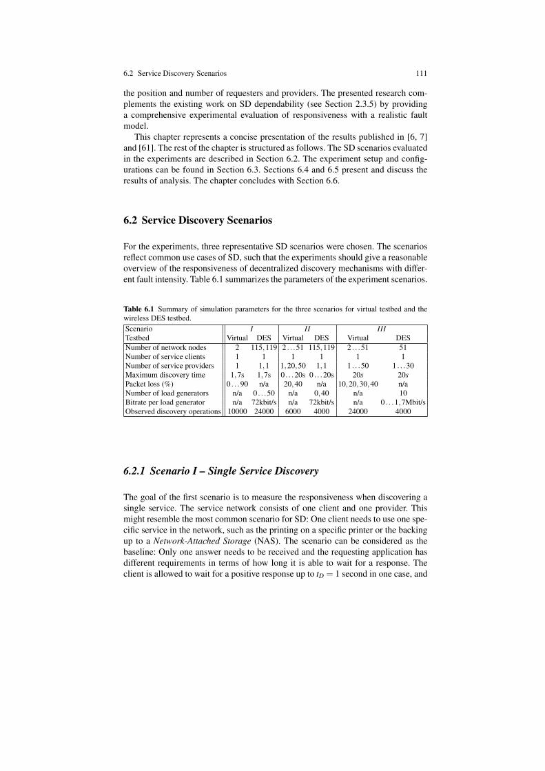
6.2 Service Discovery Scenarios 111
the position and number of requesters and providers. The presented research com-plements the existing work on SD dependability (see Section 2.3.5) by providinga comprehensive experimental evaluation of responsiveness with a realistic faultmodel.
This chapter represents a concise presentation of the results published in [6, 7]and [61]. The rest of the chapter is structured as follows. The SD scenarios evaluatedin the experiments are described in Section 6.2. The experiment setup and config-urations can be found in Section 6.3. Sections 6.4 and 6.5 present and discuss theresults of analysis. The chapter concludes with Section 6.6.
6.2 Service Discovery Scenarios
For the experiments, three representative SD scenarios were chosen. The scenariosreflect common use cases of SD, such that the experiments should give a reasonableoverview of the responsiveness of decentralized discovery mechanisms with differ-ent fault intensity. Table 6.1 summarizes the parameters of the experiment scenarios.
Table 6.1 Summary of simulation parameters for the three scenarios for virtual testbed and thewireless DES testbed.Scenario I II IIITestbed Virtual DES Virtual DES Virtual DESNumber of network nodes 2 115,119 2 . . .51 115,119 2 . . .51 51Number of service clients 1 1 1 1 1 1Number of service providers 1 1,1 1,20,50 1,1 1 . . .50 1 . . .30Maximum discovery time 1,7s 1,7s 0 . . .20s 0 . . .20s 20s 20sPacket loss (%) 0 . . .90 n/a 20,40 n/a 10,20,30,40 n/aNumber of load generators n/a 0 . . .50 n/a 0,40 n/a 10Bitrate per load generator n/a 72kbit/s n/a 72kbit/s n/a 0 . . .1,7Mbit/sObserved discovery operations 10000 24000 6000 4000 24000 4000
6.2.1 Scenario I – Single Service Discovery
The goal of the first scenario is to measure the responsiveness when discovering asingle service. The service network consists of one client and one provider. Thismight resemble the most common scenario for SD: One client needs to use one spe-cific service in the network, such as the printing on a specific printer or the backingup to a Network-Attached Storage (NAS). The scenario can be considered as thebaseline: Only one answer needs to be received and the requesting application hasdifferent requirements in terms of how long it is able to wait for a response. Theclient is allowed to wait for a positive response up to tD = 1 second in one case, and

112 6 Experimental Responsiveness Evaluation
up to tD = 7 seconds in the other. These deadlines were chosen as they correspondto two retry events in the Zeroconf discovery protocol, which was used in the exper-iments. As can be seen in Table 2.1, the first retry is triggered at tD = 1 second andthe third retry at tD = 7 seconds. Due to delays on the nodes and in the network, wecan be sure that in the first case only responses to a single request arrived while inthe second case three requests have been sent.
To see how results vary in unreliable networks, measurements are taken withincreasing fault intensity. In the virtual testbed, packet loss rates are varied from 0to 90 percent. In the wireless testbed, additional load is generated increasing from0 to 50 streams with a data rate of 72 kilobits per second each. We additionallyanalyze providers at two different positions in the WMN to investigate the impactof distance on responsiveness.
6.2.2 Scenario II – Timely Service Discovery
Many service networks are populated with multiple instances of the same servicetype to support redundancy. A client needs to discover as many instances as possi-ble and will then choose one that optimally fits its requirements or failover to an-other provider later in case the chosen one crashes. For consistent conditions, in thisscenario full coverage is required, so all available providers need to be discovered.There is one service client, P service providers with P ∈ {1,10,50} and discoveryis successful when all p = P provided service instances have been discovered. Thegoal is to measure how responsiveness increases with time. It should be obvious thatthe faster a required responsiveness can be reached, the better.
In the virtual environment, measurements are carried out with a packet loss rateof 20 and 40 percent, respectively. In the testbed, we use two different load setups, 0to 40 streams with the same data rate of 72 kilobits as in Section 6.2.1. Additionally,instead of trying to discover multiple providers, we fix P = 1 and analyze providersat two different positions in the WMN to demonstrate the impact of distance onR(t).
6.2.3 Scenario III – Multiple Service Discovery
When dealing with diverse faults in the network, having more redundant instancesof a given service type should generally increase SD responsiveness when lookingfor a fixed number of instances. In the case of fixed coverage however, which meansthe ratio of discovered services needed for successful operation remains constant,this is not necessarily the case. Fixed coverage is needed, for example, for monitor-ing tasks or in general, when complete knowledge about available service providersis demanded. A more thorough investigation of the improvements to responsivenesswhen deploying more service providers is justified. The impact of additional com-

6.3 Experiment Setup 113
munication overhead when discovering an increasing number of providers remainsunclear.
This is why in the third scenario, we investigate the difference in responsivenesswhen discovering p = P out of P service instances (full coverage). In the virtualtestbed, P is growing from 1 up to 50 providers. Measurements are carried outwith a packet loss rate of 10,20,30 and 40 percent. The experiments in the DEStestbed were run in the dense cloud of building T9 of the DES testbed (see Section6.3.2) as the increasing load would quickly cause bridging links between the build-ings to break down, partitioning the network and rendering results useless. This re-duced the total number of network nodes. The maximum number of providers hereis max(P) = 30. Also, instead of setting a packet loss rate, we are increasing theload in the network until a saturation point where responsiveness does not decreaseanymore.
6.3 Experiment Setup
In this section, the setups for the two experiment platforms, the virtualized envi-ronment and the wireless DES testbed, are explained, to carry out the experimentsneeded for the scenarios described in Section 6.2. We focus on the most importantparameters. More detailed information about the experiments can be found in [6, 7],the ExCovery framework is described in Chapter 3.
As service discovery protocol, the wide-spread Zeroconf protocol suite based onmulticast DNS [54] and DNS-based service descriptions [53] is used. A full de-scription of the protocol can be found in [55]. Zeroconf implements a two-partyarchitecture (see also Section 2.2.1) and all messages, requests and responses, aresent via multicast. Comparable experiments were carried out using Service Loca-tion Protocol (SLP). Since the results for SLP confirm the findings shown here forZeroconf , they are not included in this Chapter and can be found in [61].
Discovery requests are run from a single dedicated discovering node – or ser-vice client. All other nodes act as service providers forwarding and/or respondingto discovery requests. A discovery operation consists of an initial request and a se-ries of retries if an insufficient number of responses is received until a timeout. Foreach provider, only a single response packet needs to arrive at the requester. Givena total number of P providers, an operation to discover p providers is successful,when p providers have received at least one request packet and from each of thesep providers one response has arrived at the requester within deadline tD. The prob-ability of a request to arrive at p providers and of p responses from those providersto arrive until tD at the requester denotes the responsiveness R(tD) of the discoveryoperation. The minimum of multicast messages to be sent is p+ 1, not includingduplicate transmissions in the network due to the multicast flooding. Consequently,the maximum number of messages for each request and subsequent retry is P+ 1.It needs to be pointed out that the actual number of transmissions inside the meshnetwork is considerably higher and grows with an increasing number of collisions.

114 6 Experimental Responsiveness Evaluation
Discoveries were aborted and considered failed if no responses arrived until anexperiment run deadline of max(tD) = 20 seconds in the virtual testbed, respectivelymax(tD) = 30 seconds in the wireless testbed. This value was chosen because in Ze-roconf , the time between retries doubles after each retry to reduce network load (seealso Section 2.2.2 and Table 2.1). So after 15 seconds, we have reached a total num-ber of five SD requests and the next one would be sent after 31 seconds. Waitingtime was extended by additional 5 seconds in the XeN environment to ensure de-livery of all responses. In the wireless testbed, the extension was 15 seconds. Sinceno considerable delay was to be expected in the virtual testbed, the shorter dead-line is justified. In both cases, the timeout means that for Zeroconf we will have theresponsiveness after four retries at max(tD).
6.3.1 Virtual Testbed
All experiments in the virtual testbed were carried out on a machine running theXen hypervisor [188]. Service provider and client nodes ran as unprivileged guestdomains [27]. Provider nodes had the same base system to boot from, which wasa minimal installation of the Debian Linux operating system [75]. At boot time,they were only running the Zeroconf daemons to configure the service networkand do SD. A dedicated client node additionally ran a Secure SHell (SSH) daemonfor remote execution of discovery operations. Memory requirements for the guestsystems were very low, the technical specifications of the systems are listed in Table6.2. A schematic of the virtual testbed setup is shown in Figure 6.1.
Table 6.2 Technical specification of simulation systems
Xen host Zeroconf nodes
Processor type Intel Xeon X5365 n/a
Processor frequency 3000 Mhz n/a
Cores 2∗4 1
Memory 16 GB 48 MB
Operating system Linux openSUSE 11.0 Linux Debian 5.0.3
Architecture x86 64 x86 64
Kernel version 2.6.25.20-0.5-xen 2.6.26-2-xen-amd64
Xen version 3.2.1 16881 04-4.3 n/a
Avahi version n/a 0.6.23-3lenny1
The service network for the nodes was realized by connecting them to a virtualnetwork bridge on the Xen host. This network was solely used for SD communi-cation. On the Internet Protocol (IP) [187] layer, the topology reflects a fully con-nected, single-hop network. All packets sent among nodes pass the bridge betweenthem. On this bridge, packet loss was realized by randomly dropping packets at a

6.3 Experiment Setup 115
XeN Host
SSH
client
SSH
provider 1bridge
provider n
provider 0…
Experi-ment Script
Without packet loss
With packet loss
Fig. 6.1 Overview of the virtual testbed setup.
given rate. The rate was the same for every packet, no additional faults were injectedon the bridge. Packet dropping was done independently in the forwarding directionof every individual interface connected to the virtual bridge. The setup causes mul-ticasts or broadcasts to be potentially lost at the interface to every node they weretransmitted to. This effectively prevents all-or-nothing behavior where a broadcastis either received by all or by no host at all. A multicast can be lost on the way to onenode without affecting the probability of getting lost on the way to any of the othernodes. The SSH daemon on the client node ran on a second interface which was notconnected to the virtual bridge so that it was unaffected by the fault injection andtraffic on this interface did not interfere with service network traffic.
To automatically configure the service network, software developed by the Avahiproject [22] was used. Avahi is an implementation of the protocols recommendedby the Zeroconf working group for automatic configuration of IP service networks[243]. An Automatic private IP addressing (AutoIP) [52] daemon set a unique IPaddress within the 169.254.0.0/16 subnet and an mDNS [54] daemon handled ser-vice name resolution for DNS-based service discovery [53]. Due to the fact thatAvahi was used for auto-configuration, all nodes could run from copies of the samesystem disk image and no manual administration was necessary after booting. Dur-ing measurements, no nodes joined or left the network so no reconfiguration of thenetwork layers occurred which could interfere with the observed SD operations.
In the XeN environment, discovery times were measured on the client directlybefore the request was sent and directly after responses were received to measureuser-perceived responsiveness. Thus, time synchronization between nodes in theservice network was not necessary.

116 6 Experimental Responsiveness Evaluation
Justification of Experiment Setup
The chosen network model is a simplified version of a fully connected, wired Eth-ernet network. In such reliable networks, packet loss is usually not an issue. Typicalunreliable networks, especially wireless networks as in the second testbed, havea complex fault behavior. Most faults occurring in these networks, such as burstsof packet loss, delay or jitter have complex functional dependencies. However, theintention behind using this virtual testbed is to control the network faults duringexperiments as much as possible to isolate their impact.
Packet loss is expected to be among the highest-impact faults in SD. Thus, theexperiments run in this testbed focus on packet loss. The fault model includes onlyrandom packet loss at a given rate, independent of the traffic occurring on the linkand whether preceding packets are lost as well. Packet delivery time, which is inthe order of hundreds of microseconds in this testbed, can be neglected comparedto the time between discovery retries, which is in the order of seconds (see Ta-ble 2.1). Since an average packet loss is assumed, service discovery responsivenesswill most probably be worse in networks with the same packet loss rate but morecomplex fault characteristics. This analysis hence provides an upper bound for re-sponsiveness which will be compared to the results in the wireless DES testbed withhighly complex fault characteristics.
6.3.2 Wireless Testbed
As the second platform to execute experiments, the wireless DES-Testbed at FreieUniversitat Berlin (FUB) was used. To run the experiments, the ExCovery frame-work for distributed system experiments was employed. ExCovery was specificallydeveloped for this work and supports the DES testbed as the first experiment plat-form. More in-depth information on ExCovery follows in Chapter 3.
The DES testbed consists of roughly 130 uniform nodes equipped with IEEE802.11 hardware. The nodes are spread indoors and outdoors over three adjacentcampus buildings at FUB. An overview of the testbed topology is depicted in Figure6.2 which shows the geographical location of the nodes in buildings a3, a6 and t9.Nodes have been color-coded to distinguish the different building floors. Specialnodes that are the focus of the following analysis are labeled with their identificationstring. Wireless network links have been left out for reasons of visibility. While themesh network forms reasonably dense clouds within the buildings, the connectionsbetween buildings are not optimal. Building a6 and t9 are connected by several linksbut a3 and a6 are often only connected by a single bridge, depending on the overallwireless signal quality. More in-depth information about the properties of the DEStestbed can be found in [36, 100, 101].
The DES testbed was chosen for various reasons. First of all, as opposed to thevirtual environment, it allows to evaluate processes in a network with realistic faultbehavior. Second, the DES testbed allows to generate manifold topologies due to

6.3 Experiment Setup 117
Fig. 6.2 Overview of the wireless DES testbed. Three buildings can be distinguished, nodes colorsdefine their building floors.
its wide distribution of nodes on campus and the ability to manipulate their wire-
less signal range. This gave us the possibility to study in detail the effects of node
distance on SD responsiveness. Finally, the nodes run a relatively modern Linux
distribution which simplifies the development and deployment of new software.
Multicast provides considerable challenges in wireless mesh networks, which
need to rely on costly flooding mechanisms to deliver these messages. Nevertheless,
Zeroconf was developed for mobile and dynamic networks and both its focus and
prominence make it a prime target for examination. Just as for the experiments in the
virtual testbed, Avahi [22] was used to implement SD, albeit in a slightly newer ver-
sion 0.6.29. However, the results presented in Sections 6.4 and 6.5 provide insight
also in the behavior of other SD protocols, which implement the same operations,
as will be discussed later.
The experiments have been run in three series from May 2013 to May 2014. Each
series took several weeks to complete, due to the overhead involved when carrying

118 6 Experimental Responsiveness Evaluation
out experiments. Every single discovery operation needs to be initialized properly,measured and cleaned up. Since the setup is slightly more complex than in the XeNtestbed, we will detail a few of those steps below. It should be noted, however, thatthe ExCovery framework takes care of most of the steps during the actual executionof experiments.
Experiment Initialization
During initialization, the SD daemons are started on all providers. Then, all SDpackets are dropped on all nodes for a specific period to prevent service announce-ments and delayed responses from previous runs on the network. After dropping,the load generation is started. To simulate additional load on the network, environ-ment nodes are chosen randomly to exchange UDP [186] packets at a given datarate. UDP is chosen due to its ”send and forget” strategy, to be able to control thedata rate at the given level without corrective measures such as flow and congestioncontrol.
Experiment Measurement and Cleanup
During the measurement phase, the SD process is started and SD packets capturedas well as defined SD events recorded, such as ”search started” or ”provider found”.Either when a required number of providers has been found or the deadline of 30seconds has been reached, the measurement phase ends and cleanup starts, whereload generation is stopped and SD daemons are shut down. Due to the long time-outs of current SD protocols and the overhead involved, one experiment run usuallytakes between 45 and 90 seconds to complete. Runs can be rendered invalid due tocomplete network outages or missing connectivity on too many actor nodes of thediscovery operation. While requesters had to be connected at any time to producevalid results, we decided that up to 10 percent of providers where allowed to betemporarily disconnected. This means that the actual number of SD operations thatwere carried out was considerably higher than the number shown in Table 6.1.
Scenario-Specific Setups
The first two series of experiments cover the discovery of a single provider by asingle client as in the scenario from Section 6.2.1 and in parts, from Section 6.2.2.In both series, the requesting node was t9-105. In one series the provider was t9-154to cover scenarios where both nodes are in the same building, thus, in one well con-nected cloud. In the second series the provider was a3-119 at a maximum hop dis-tance to t9-105 to study the effects on SD responsiveness in scenarios where nodesare connected with sparse and possibly weak links. All other nodes participated in

6.3 Experiment Setup 119
Table 6.3 Experiment configuration of each series
Experiment Series I Series II Series III
Number of nodes (max) 115 119 51
Nodes in buildings t9, a3, a6 t9, a3, a6 t9
Number of requesters 1 (t9-105) 1 (t9-105) 1 (t9-154)
Number of responders 1 (a3-119) 1 (t9-154) 1 . . .30
Number of load generators 0 . . .50 0 . . .50 10
Bitrate per generator (kbit/s) 72 72 0 . . .1725
randomly distributed load generation at various levels. The position of nodes within
the network is depicted in Figure 6.2.
A separate series of experiments for the scenario from Section 6.2.3 was carried
out only in the dense cloud of building t9. Requester t9-154 was trying to discover
up to 30 service providers while the remaining nodes generated load in the network.
The topology of these experiments is illustrated in Figure 6.3. Nodes can be distin-
guished by their form and color. Again, the colors define the three building floors
the nodes reside on. The shapes define the node type: Circle nodes are providers,
cross nodes are environment nodes used for load generation.
Fig. 6.3 Overview of building t9 of the wireless DES testbed. Nodes colors define their build-ing floors. Circle nodes are providers, crosses denote environment nodes for load generation. Therequester t9-154 has been labeled.
The most important configuration parameters of the three experiment series are
summed up in Table 6.3.

120 6 Experimental Responsiveness Evaluation
6.4 Experiment Results
We will now present and discuss the results for the behavior of R(tD) under vary-ing influences, as described in the three scenarios in Section 6.2. Each scenario wasrepeatedly run and observed in a series of experiments. In the virtual testbed exper-iments, the total number of experiment runs amounted to 60,000. This equals thenumber of discovery operations for all scenarios combined, hence it is equal to thenumber of discovery requests without retries. The number of accumulated discoveryresponses reached 599,046 over all runs. Requests were split equally over loss ratesranging from 0% to 90% in 10% steps and over the number of provided service in-stances equal to 1,2,5,10,20 and 50. A subset of these results was investigated forthe defined SD scenarios, as shown in Table 6.1. The total number of experimentruns in the wireless testbed series was 32004 of which 26670 provided valid resultsfor analysis. Due to the overhead involved in running those experiments, the seriestook several weeks to complete. The conditions for the validity of runs are explainedin Section 6.3.2.
To foster repeatability, the raw measured data of all experiments in the XeNtestbed has been uploaded to the AMBER Data Repository [149]. Interested re-searchers are invited to validate the results and perform further investigations. Thefull experiment data of the DES experiments, including experiment description,packet and event logs and all other measurements as explained in Chapter 3 areavailable for examination on request.
6.4.1 Scenario Results – Single Service Discovery
This analysis investigates in more detail how R(tD) for tD ∈ {1,7} seconds decreaseswith an increasing fault intensity in the network. According to the results in the vir-tual testbed, discovery of single service providers within the deadline tD = 7 secondsproved to be reasonably responsive in networks with low packet loss. As illustratedin Figure 6.4, even with 30% packet loss, the responsiveness of single service dis-covery was well above 0.9 for the given deadline. Keeping in mind the focus of thisscenario with lax requirements for the deadline, this is most probably also true forthe required responsiveness. Considering a consumer context, such as home officeor entertainment, a higher than 90% probability of success seems sufficient.
With higher packet loss rates, responsiveness decreases rapidly, dropping to 0.63at 50 percent packet loss. In real world networks with more complex fault behavior,for example wireless networks, the results are expected to be worse, which is notpromising for use cases with stricter requirements. However, it is valid to concludethat given a deadline tD = 7 seconds, with up to 20 percent packet loss and noadditional negative effects, single service discovery is sufficiently responsive.
The picture is a different one for tD = 1 second. Here, at a packet loss rate of30%, a service will only be discovered every second try. The curve for R(1) per-fectly represents the expected behavior for discovery without retries. Since for SD

6.4 Experiment Results 121
Fig. 6.4 Responsiveness of single service discovery with deadline tD = 1,7 seconds as a functionof packet loss rate.
to be successful, both the request and the subsequent response need to arrive at theirdestinations. Given a packet loss rate of Ploss in each direction, both packets arrivewith a probability of 1−Ploss. So R(1) may also be calculated using Equation 6.1.Values calculated by Equation 6.1 are listed in Table 6.4. They almost perfectlymatch the results from the experiment series in Figure 6.4. This validates the cho-sen experiment setup. With a more realistic fault model and an arbitrary number ofretries, the calculation of responsiveness gets considerably more complex. Chapter7 will present a hierarchy of stochastic models to do so.
R(1) = (1−Ploss)2 (6.1)
Table 6.4 Expected responsiveness with a given packet loss rate for discovery without retries.
Packet Loss Rate 0% 10% 20% 30% 40% 50% 60% 70% 80% 90% 100%
R(1) 1 0.81 0.64 0.49 0.36 0.25 0.16 0.09 0.04 0.01 0
In the wireless testbed, the results paint a comparable picture, although the dif-ferences are worth being explored. For this, R(tD) with tD ∈ {1,7} was calculatedfor each load level. The results are illustrated in Figure 6.5. The figures show forthe two providers t9-154 and a3-119 how R(tD) decreases with increasing load. Thecurves in the figures are the regression functions over all data points of a specificprovider.
Comparable is for both providers that until a certain point, the responsiveness de-creases but does not drop to quickly. Depending on the distance from the requester,
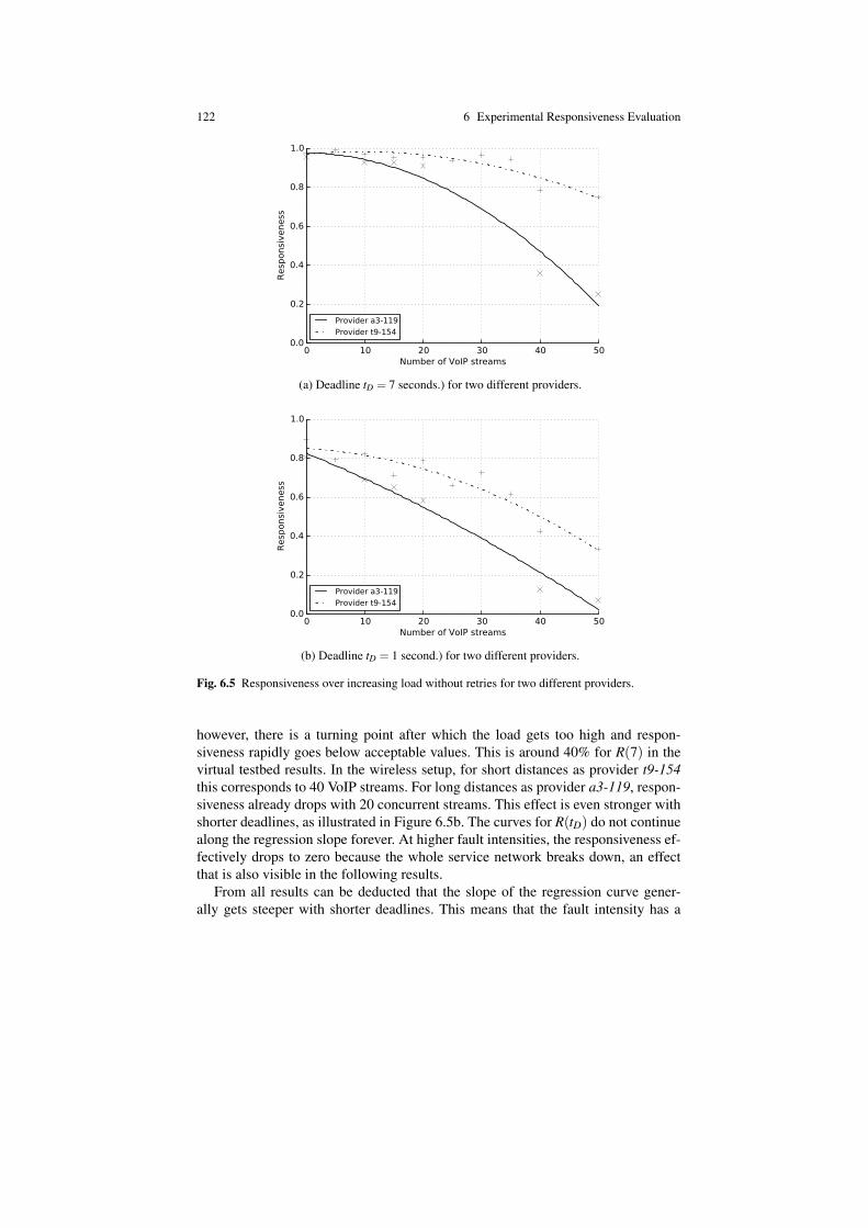
122 6 Experimental Responsiveness Evaluation
(a) Deadline tD = 7 seconds.) for two different providers.
(b) Deadline tD = 1 second.) for two different providers.
Fig. 6.5 Responsiveness over increasing load without retries for two different providers.
however, there is a turning point after which the load gets too high and respon-siveness rapidly goes below acceptable values. This is around 40% for R(7) in thevirtual testbed results. In the wireless setup, for short distances as provider t9-154this corresponds to 40 VoIP streams. For long distances as provider a3-119, respon-siveness already drops with 20 concurrent streams. This effect is even stronger withshorter deadlines, as illustrated in Figure 6.5b. The curves for R(tD) do not continuealong the regression slope forever. At higher fault intensities, the responsiveness ef-fectively drops to zero because the whole service network breaks down, an effectthat is also visible in the following results.
From all results can be deducted that the slope of the regression curve gener-ally gets steeper with shorter deadlines. This means that the fault intensity has a

6.4 Experiment Results 123
higher impact on R(tD) the less time there is to complete the discovery operation.In wireless networks, one reason for this behavior is the impact of delay on R(tD).However, this effect is not existent in the virtual testbed and warrants more in-depthevaluation in future research.
6.4.2 Scenario Results – Timely Service Discovery
The results in this section present responsiveness with increasing deadlines. Theanalysis of the virtual testbed data is illustrated in Figure 6.6. The characteristicsteps in the curves mark the request retry events. Conforming to the fault model, acertain amount of requests and responses gets lost, so after each discovery requestthe responsiveness curve plateaus until the retry timeout, when a new request isbeing sent.
With 20% packet loss, the responsiveness of discovering a single service ap-proaches 1 within the observed interval (Figure 6.6a). This corresponds to the con-clusions from single SD at 7 seconds waiting time (see Figure 6.4). In fact, in thisscenario discovering a single service reaches a responsiveness of almost 0.9 alreadyafter the first retry, after roughly one second. We can conclude that with low packetloss, current SD protocols work sufficiently well when discovering single serviceinstances.
However, Figure 6.6a also shows that responsiveness decreases rapidly if moreservices need to be discovered. Both discovering 10 and 50 service instances reachesa somewhat acceptable (≈ 0.95 and≈ 0.7) responsiveness at the end of the timescaleafter four retries with 20 percent packet loss. This corresponds to use cases whenthere is enough time to wait for discovery responses and, especially in the case of50 instances, low responsiveness is acceptable. Those cases are expected to be rarein regular service networks. If short response times are needed, as they are for theuse cases anticipated in the Internet of Things, we need a high responsiveness inshortest time. It can be seen in Figure 6.6a that both curves require a long discoverytime, thus, a high deadline tD to reach reasonable responsiveness.
With 40 percent packet loss, discovery of multiple services becomes highly im-probable. Figure 6.6b illustrates this. There is a chance of less than 1/3 to find allservices instances in time when there are 10 instances in the network. Discovering50 service instances is practically impossible. In contrast, discovering single ser-vices remains partly usable so doubling the packet loss rate did not have such acomparable dramatic effect on responsiveness as with multiple services. This dra-matic decrease in responsiveness when discovering more service instances will befurther investigated in the next scenario in Section 6.4.3. The observed behavior isbacked up by analytical evaluation. If we extend Equation 6.1 to the discovery ofmultiple service instances, with n being the number of instances, Equation 6.2 cal-culates the responsiveness at tD = 1 second, just before the first retry would get sent.

124 6 Experimental Responsiveness Evaluation
(a) Packet loss 20%
(b) Packet loss 40%
Fig. 6.6 Responsiveness over time for a different number of providers.
This means that with a rate of Ploss = 0.4, R(1) for n = 10 and n = 50 is 3.6 ·10−3
and 4.85 ·10−12, respectively.
R(1) = (1−Ploss)1+n (6.2)
It can be expected that a shorter time between retries should significantly increaseresponsiveness at a given time t. However, this would also increase network loadand might have other adverse effects on the network especially when dealing with ahigh number of service instances, thus, a high number of discovery responses. With-out a more realistic network and fault model and a sound cost function for packettransmission it remains rather difficult to determine an optimal trade-off betweenresponsiveness and discovery packet load.

6.4 Experiment Results 125
Using the results from experiments in the wireless testbed, we now examine howR(tD) increases with tD, depending on the distance between requester and providerand the load in the network. To be able to isolate the effect of node positions onthe results, only data from experiment Series I and II was used (see Section 6.3.2and Table 6.3). Thus, the discovery operations were carried out by only two actors,one requester t9-105 and one provider: t9-154 for a short distance and a3-119 forthe maximum distance in the network. The respective node positions are depicted inFigure 6.2. All DES testbed nodes participated in routing network packets.
Figures 6.7 and 6.8 illustrate the results. Figure 6.7 shows the responsiveness ofthe discovery operation over time, equivalent to Figure 6.6, for providers t9-154 anda3-119. Also in the testbed the two curves in each graph reflect the responsivenessfor different load conditions. As expected, responsiveness increases with every re-quest being sent, which corresponds to the steps in the curves. It can be seen thatR(tD) is generally lower with higher distance. It can further be noted that additionalload in the network has a dramatic effect on the packet loss rates and consider-ably decreases R(tD). The 40 VoIP streams are randomly distributed in the network,changing each experiment run. They impose a combined load of 2.8Mbit/s, whichdoes not seem much compared to the maximum theoretical data rates in the net-work. Still, even with tD = 18s there is only a 50% chance of discovering providera3-119 under these conditions. However, packet loss is not the only factor impactingR(tD). Especially at higher loads, the delay of individual packets becomes apparent,smoothening the steps in the curve. This effect is also visible in Figure 6.7b forprovider a3-119.
The results are in line with the ones from the virtual testbed. The current SDprotocol retry configuration works well when conditions are close to perfect buttheir responsiveness decreases significantly when conditions deteriorate. Their staticretry strategies struggle in unreliable networks. As can be seen later, the analyticalmodels in Chapter 7 hint at possible advantages in conditions when SDPs (namelySLP [106] and SSDP [93]) use the more reliable unicast instead of multicast forcertain messsages.
Packet Based Analysis
The discovery operation of a single service consists of multiple pairs request andresponse. Figure 6.8 shows the responsiveness of such individual packet pairs withinan SD operation. Here, R(tD) denotes the probability that a response to a givenrequest arrived within tD. The characteristics of the curves confirm the findings onR(tD) for the complete discovery operation, with R(1) being roughly the same forthe corresponding graphs of each provider (Figures 6.7a and 6.8a, respectively 6.7band 6.8b). The results are included here because they are not based on the eventsas measured on the discovery layer but instead use raw packet captures done byExCovery. As such, ExCovery supports diverse analysis types using the same resultdatabase. Packet response times as in Figure 6.8 can be used, for example, as lowerlevel input data in the analytical responsiveness models presented in Section 7.2.1
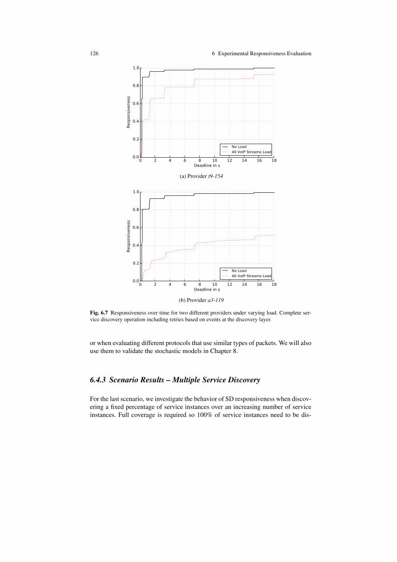
126 6 Experimental Responsiveness Evaluation
(a) Provider t9-154
(b) Provider a3-119
Fig. 6.7 Responsiveness over time for two different providers under varying load. Complete ser-vice discovery operation including retries based on events at the discovery layer.
or when evaluating different protocols that use similar types of packets. We will alsouse them to validate the stochastic models in Chapter 8.
6.4.3 Scenario Results – Multiple Service Discovery
For the last scenario, we investigate the behavior of SD responsiveness when discov-ering a fixed percentage of service instances over an increasing number of serviceinstances. Full coverage is required so 100% of service instances need to be dis-

6.4 Experiment Results 127
(a) Provider t9-154
(b) Provider a3-119
Fig. 6.8 Responsiveness over time for two different providers under varying load. Packet-basedanalysis for individual discovery request and response pairs.
covered for successful operation. All instances belong to the same service type –a single discovery request should discover all instances if no packets are lost. Thisconfiguration reflects basically any SD scenario where a client tries to enumerateas many service providers of a given service class as possible to select the best nproviders according to its requirements. It could already be deduced from the pre-vious scenario that SD responsiveness decreases dramatically when discovering tenor more services in lossy networks. Figure 6.9 shows an articulate explanation forthis behavior.
With low packet loss rates responsiveness decreases almost linearly with thenumber of nodes in the network. This is the reason why with 20% packet loss we
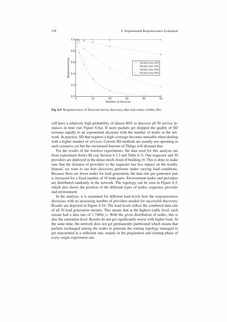
128 6 Experimental Responsiveness Evaluation
Fig. 6.9 Responsiveness of Zeroconf service discovery after four retries (within 20s)
still have a relatively high probability of almost 80% to discover all 50 service in-
stances in time (see Figure 6.6a). If more packets get dropped the quality of SD
worsens rapidly to an exponential decrease with the number of nodes in the net-
work. In practice, SD that requires a high coverage becomes unusable when dealing
with a higher number of services. Current SD methods are usually not operating in
such scenarios yet but the envisioned Internet of Things will demand that.
For the results of the wireless experiments, the data used for this analysis are
from experiment Series III (see Section 6.3.2 and Table 6.3). One requester and 30
providers are deployed in the dense mesh cloud of building t9. This is done to make
sure that the distance of providers to the requester has less impact on the results.
Instead, we want to see how discovery performs under varying load conditions.
Because there are fewer nodes for load generation, the data rate per generator pair
is increased for a fixed number of 10 node pairs. Environment nodes and providers
are distributed randomly in the network. The topology can be seen in Figure 6.3,
which also shows the position of the different types of nodes, requester, provider
and environment.
In the analysis, it is examined for different load levels how the responsiveness
decreases with an increasing number of providers needed for successful discovery.
Results are depicted in Figure 6.10. The load levels reflect the combined data rate
of all 10 load generation streams. This means that at the highest traffic level, each
stream had a data rate of 1.7Mbit/s. With the given distribution of nodes, this is
also the saturation level. Results do not get significantly worse with higher load. At
the same time, the network does not get permanently partitioned which means that
packets exchanged among the nodes to generate the routing topology managed to
get transmitted at a sufficient rate, mainly in the preparation and cleanup phase of
every single experiment run.

6.5 Experiment Results of Testbed Behavior 129
0.0
0.2
0.4
0.6
0.8
1.0
Responsiv
eness
0 5 10 15 20 25 30
Number of Services
Load 0.00 Mbit/s
Load 0.70 Mbit/s
Load 2.11 Mbit/s
Load 16.88 Mbit/s
Fig. 6.10 Responsiveness over number of needed service providers for different load levels.
The results demonstrate that deploying more services is not generally a promis-
ing solution to increase responsiveness in wireless mesh networks. It confirms the
findings from the virtual testbed experiments, albeit there is no linear decrease of re-
sponsiveness with lower load. One can see that at very high loads, discovering more
than 20 nodes is impossible. Although not shown in Figure 6.10, there is an almost
identical set of discovered nodes over all runs at that load level. This is because some
nodes, although not partitioned from the rest of the network, are effectively blocked
off SD by environment nodes that are generating load at very high data rates in their
vicinity. Further research on the transmission mechanisms (unicast or multicast) and
the retry intervals is needed to optimize responsiveness in such scenarios.
6.5 Experiment Results of Testbed Behavior
Ideally, a testbed should provide a controlled environment over a series of exper-
iments. More precisely, held-constant factors should be known and accounted for
in a later analysis and the effect of allowed-to-vary factors should be minimized.
Nuisance factors with an unwanted or unknown effect on the results should be elim-
inated as much as possible. The different types of factors are described in Section
3.2.2 and more in detail in [9]. Such stable and known conditions could only be
achieved in the XeN-based virtual testbed. In the DES testbed, which is highly sen-
sitive to external interference, the different nuisance factors are both difficult to de-
termine and to measure. The probability of unwanted effects on the results is even
higher the longer it takes to run the experiments. Given that the experiments carried
out took several weeks to complete, a better knowledge of the testbed behavior is

130 6 Experimental Responsiveness Evaluation
necessary. Although we cannot determine the source of all nuisance factors, we canmeasure them and show their effect.
This section presents general measurements of the behavior of the DES testbedfor the duration of the experiments. These cover the variation of response timesunder similar conditions (see Section 6.5.1), the varying quality of individual links(see Section 6.5.2) and the clock drift of the network nodes (see Section 6.5.3) overtime. The results should illustrate the behavior of the DES testbed over time andhelp to interpret the results of the discovery process analyses shown in Section 6.4. Itshould be pointed out that results can only be representative for the scenarios whichhave been realized with the DES testbed. Uniform grid topologies, for example,cannot be created with the testbed. Thus, the significance of the results for suchscenarios needs to be inspected before drawing conclusions.
6.5.1 Response Times over All Runs
Figures 6.11 and 6.12 illustrate the effects of internal an external faults on the resultsfor a part of four sets of experiments from Series I and II (see Table 6.3). Theresponse times of discovery operations, which in this case are the times for thefirst response to arrive at the requester, are plotted over 1000 experiment runs. Therequesting node is t9-105, the providers are t9-154 (Figure 6.11) and a3-119 (Figure6.12). Nodes t9-105 and t9-154 are in one cloud within the same building while t9-105 and a3-119 cover the maximum hop distance in the network. The node positionsin the mesh network are shown in Figure 6.2. For each node pair, results are shownwithout additional load in the network (upper Figures 6.11a and 6.12a) and withan additional load of 40 Voice-over-IP (VoIP) streams with 72 kbit/s each, whichamounts to roughly 2.8 Mbit/s traffic overall in the network (lower Figures 6.11band 6.12b).
In the graphs, the dots reflect response times of individual discovery operationswhile the line denotes a moving average over 20 operations. Depending on the ad-ditional load on the network, the 1000 runs cover a period of 15− 20 hours so thegraphs are showing long-term effects in the testbed. One can see that the responsetimes generally increase with the load in the network and the distance of requesterand provider. At times 1,3,7 and 15 seconds we see a significant accumulation ofresponses. This corresponds to the default retry intervals of the Zeroconf discoveryprotocol as already visible in Figure 6.7. Zeroconf starts with a timeout of one sec-ond and then doubles this timeout on every retry (see Table 2.1). The accumulationof responses very close to the retry intervals hints at packet loss having the deci-sive impact on response times: Either packets arrive in time or they get lost. Withhigher loads and distances, however, also packet delay comes into play which is es-pecially visible in Figure 6.12b, where the accumulation at the retry intervals is lesspronounced and response times generally have a wider distribution.
While the responsiveness over load and distance has been examined in moredetail in Section 6.4, it can be noted that the response times are not independent

6.5 Experiment Results of Testbed Behavior 131
(a) Without additional load in the network
(b) With additional load of 40 VoIP streams with 72 kbit/s each
Fig. 6.11 Response times in testbed over 1000 experiment runs. Requester is t9-105, provider ist9-154 at short distance in the same cloud as the requester.
over time. There are periods of consistently higher response times, such as in Fig-ure 6.12a between runs 120 and 180 or in Figure 6.11b between runs 820 and 900.Given that these intervals span roughly an hour of experiment time, it seems highlyimprobable that these effects are random statistical accumulations. Instead, they hintat external causes that degrade the overall quality of the wireless testbed. Further-more, those events happen very frequently. Finding the root cause of such anomaliesis out of the scope of this work. The results are meant to demonstrate instead that anyanalysis based on average measurements should be done very carefully. Choosingthe measurement history window size too big can easily lead to over- or underesti-mating the testbed quality. Also, it is important to measure and store all historical

132 6 Experimental Responsiveness Evaluation
(a) Without additional load in the network
(b) With additional load of 40 VoIP streams with 72 kbit/s each
Fig. 6.12 Response times in testbed over 1000 experiment runs. Requester is t9-105, provider isa3-119 at maximum distance from the requester.
data, as does the ExCovery framework (see Chapter 3), to be able to detect andvisualize such effects.
6.5.2 Topology Changes over Time
The variations in overall response times hint at changing link qualities over time.This why the ExCovery framework supports full topology recordings including linkqualities at the end of each run in a series of experiments. More details on these
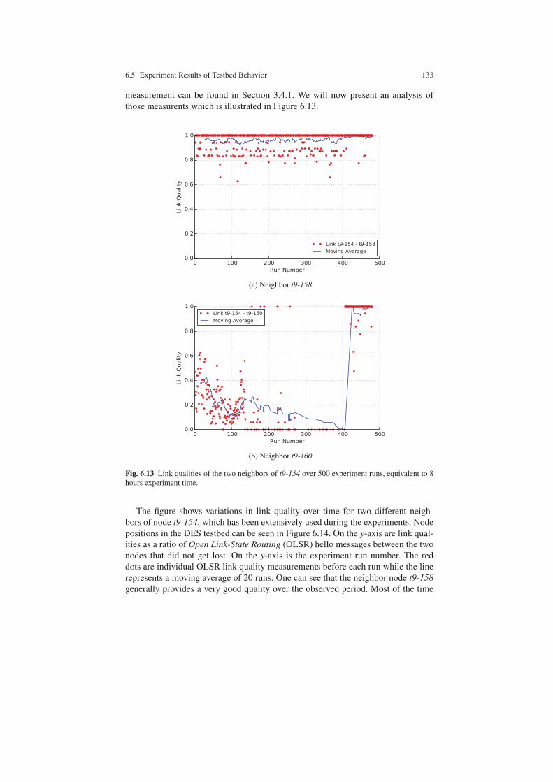
6.5 Experiment Results of Testbed Behavior 133
measurement can be found in Section 3.4.1. We will now present an analysis of
those measurents which is illustrated in Figure 6.13.
(a) Neighbor t9-158
(b) Neighbor t9-160
Fig. 6.13 Link qualities of the two neighbors of t9-154 over 500 experiment runs, equivalent to 8hours experiment time.
The figure shows variations in link quality over time for two different neigh-
bors of node t9-154, which has been extensively used during the experiments. Node
positions in the DES testbed can be seen in Figure 6.14. On the y-axis are link qual-
ities as a ratio of Open Link-State Routing (OLSR) hello messages between the two
nodes that did not get lost. On the y-axis is the experiment run number. The red
dots are individual OLSR link quality measurements before each run while the line
represents a moving average of 20 runs. One can see that the neighbor node t9-158generally provides a very good quality over the observed period. Most of the time

134 6 Experimental Responsiveness Evaluation
the hello packet loss is close to zero. Node t9-160 shows a very different behavior.
During the first 250 runs, the link quality to t9-154 is very weak. Also, the variations
in quality are very inconsistent. Until run 400 the link is basically down. Then, the
link quality suddenly becomes almost perfect and remains so until the end of the
observed period. This erratic behavior of course has an impact on the routing within
the network and thus, on the propagation of multicast packets which are the base of
SD.
Fig. 6.14 Overview of building t9 of the wireless DES testbed. Nodes colors define their buildingfloors. The node t9-154 and its neighbors t9-158 and t9-160 have been labeled.
6.5.3 Node Clock Drift over Time
While Sections 6.5.1 and 6.5.2 show the effects of external factors on the experiment
results, there are also internal factors that need to be measured. In this section, we
focus on the clocks on the individual nodes. All nodes in the network synchronize
their clocks before running experiments but to not interfere with the measurements,
this is not done anymore during experiment execution and their clocks begin to drift
apart.
Figure 6.15 shows the variations of clock offsets as measured over 1200 experi-
ment runs (approximately 20 hours) in Series III. Each of the three lines represents
the offset of a different node to requester t9-154. The lines abruptly change at the
same positions of run 175 and 480. At run 175, the experiment was interrupted for
an extended period so the clocks continued to drift apart before resuming experi-
ments. This leads to the jump in the lines in direction of the clock drift relative to
the reference node t9-154. At run 480, the experiments needed to be interrupted be-
cause the time slot in the testbed ended. The nodes were rebooted multiple times

6.6 Conclusion 135
for experiments carried out by other DES testbed users. Before restarting the series,
the nodes were manually synchronized, bringing the offset to reference node t9-154close to zero. Between those characteristic steps, the clocks steadily drift apart from
each other. However, not only does every node expectedly drift differently from the
others, the drift of the individual nodes even varies over time. This can be seen for
node t9-011, which runs faster than the reference node t9-154 until experiment run
480 but after that runs slower.
-2
-1.5
-1
-0.5
0
0.5
1
1.5
2
Tim
e o
ffset in m
s
0 200 400 600 800 1000 1200
Run Number
Node t9-011
Node t9-k63
Node t9-040
Fig. 6.15 Absolut clock differences between different providers and requester t9-154 over a dura-tion of 1200 experiment runs, approximately 20 hours.
Clock synchronization is highly important for the analysis of real-time problems,
such as SD. Given the observed behavior, it is obvious that the current testbed syn-
chronization methods are not sufficient to guarantee consistent behavior over mul-
tiple hours of testbed usage. This justifies the approach of ExCovery to measure
the time difference between the nodes on every single run. After the experiments
are done, the stored event and packet times are corrected using these offsets before
being imported to the result database for further analysis. This reduces the abso-
lute synchronization error of all nodes to the precision of the measured timestamps,
which improves measurement accuracy and reduces the likelihood of causal prob-
lems during subsequent analysis. A future improvement to ExCovery would be to
optionally support time synchronization tasks during the initialization phase of each
experiment run.
6.6 Conclusion
In this chapter, we examined decentralized Service Discovery (SD) in experiments
with different fault intensities to get an initial idea about the behavior of SD re-
sponsiveness. Two experiment environments were setup to observe three common

136 6 Experimental Responsiveness Evaluation
scenarios. A virtual testbed with a fault model that includes only packet loss and theDistributed Embedded Systems (DES) wireless testbed at Freie Universitat Berlin.Analysis in the DES testbed was performed both for the individual discovery pack-ets as well as the complete discovery operation, which includes retries in case pack-ets do not arrive in time. The former allows to infer conclusions for other appli-cation protocols which use similar packets and can provide input for existing andfuture analytical models which use lower network level measurements. This will bedemonstrated in Chapter 8.
Second, an analysis of the long-term testbed behavior and the effects of internaland external faults has been carried out. Internal faults contain node crashes or clockdrifts, external faults comprise all types of wireless interference or also forced in-terruptions during experiment execution. It has been shown that the effect of thesefaults is considerable and has to be taken into account when interpreting resultsgathered in the testbed.
Chapter 7 provides a hierarchy of stochastic models to evaluate user-perceivedresponsiveness of SD. Parts of the results presented in this work are used to validatethe presented models in Chapter 8. Comparable experiments were carried out usingService Location Protocol (SLP). They confirm the results shown here for Zeroconfand have been left out for reasons of brevity. More information about these SLPexperiments can be found in [61].

Chapter 7Modeling Service Discovery Responsiveness
Abstract The focus of this work is the responsiveness of the discovery layer, theprobability to operate successfully within a deadline, even in the presence of faults.This chapter proposes a hierarchy of stochastic models to evaluate responsivenessof decentralized discovery. The models are used to describe the discovery of a sin-gle service using three popular protocols. Furthermore, a methodology to use themodel hierarchy in Wireless Mesh Networks (WMNs) is introduced. Given a pairrequester and provider, a discovery protocol and a deadline, the methodology gen-erates specific model instances and calculates responsiveness. To estimate the be-havior of multicast communication, which is fundamental to all current protocols,the methodology uses the Monte Carlo method Probabilistic Breadth-First Search(PBFS). PBFS accurately approximates multicast behavior in WMNs and it doesso with low time and space complexity compared to existing approaches. Finally,this chapter introduces a new metric, the expected responsiveness distance der, toestimate the maximum distance from a provider where requesters can still discoverit with a required responsiveness. Using monitoring data from the DES testbed atFreie Universitat Berlin, it is shown how the models can be used to calculate respon-siveness and der of current discovery protocols depending on the position of nodesand the link qualities in the network.
7.1 Introduction
This chapter provides a hierarchy of stochastic models to evaluate responsiveness ofdecentralized Service Discovery (SD) in unreliable networks. It provides a method-ology to apply these models to Wireless Mesh Networks (WMNs). The stochasticmodel hierarchy and the Monte Carlo method Probabilistic Breadth-First Search(PBFS) to estimate the reachability of multicast packets have been discussed in[4, 11]. This chapter refers to these publications where necessary and provides acomprehensive overview of how the different contributions are interconnected.
137

138 7 Modeling Service Discovery Responsiveness
The remainder of this chapter is structured as follows. A hierarchy of stochasticmodels to evaluate SD responsiveness is introduced in Section 7.2, followed bythe description and validation of the multicast estimation method PBFS in Sections7.3 and 7.4, respectively. An overview of a methodology that creates and solvesthe models can be found in Section 7.5. The case study in Section 7.6 shows theresponsiveness of SD in different scenarios as calculated by the models. Results areexplained and interpreted. Section 7.7 concludes the work.
7.2 A Model for Service Discovery
When doing SD, the number of requesters and providers may vary. For instance,multiple clients might request a single service. One client could discover all exist-ing providers in the network to choose one meeting best its requirements. We willnow focus on decentralized SD by a single client as it is the basis of all other SD op-erations. Any such SD operation can be described with a generic family of Markovmodels, which includes three types of states:
• A single state named req0 defines the beginning of the SD operation, when theinitial request has been sent.
• Two absorbing states ok and error define the successful or unsuccessful end ofthe SD operation.
• A set containing every state between the first two types where not all requiredresponses have been received and the final deadline has not been reached.
The Markov model family is parametric in two parameters: number of retries andrequired coverage. The maximum number of retries n describes the first dimensionof the model family. Beginning from the initial state req0, the retries define a chainof retry states reqi, i = 1...n, that stand for “retry i has been sent”. From each retrystate the model can transition into ok in case a sufficient number of responses wasgathered. If not it will transition to the next retry state and eventually from reqnto error. The second parameter required coverage describes how many responsesneed to be received before an SD operation is called successful and is the seconddimension of the model family. Each of the retry states reqi, i = 1...n becomes a setof states reqi j, j ≥ 1, depending on the success ratio when doing retry i. The sizeof this set may be arbitrary but as an example, if three services need to be foundfor successful operation, there could be three states reqi j, j = 0,1,2 for every retryi that stand for “retry i has been sent and j responses have been received so far”.Figure 7.1 exemplary depicts a model in this family with two retries and three statesto reflect the different success ratios.
Estimating the transition probabilities within this Markov model family is nottrivial. In the following, we propose a hierarchy of stochastic models where theprobabilities of these high level discovery models are calculated by low level modelsbased on link quality data measured in the network. The hierarchy consists of thefollowing three layers:
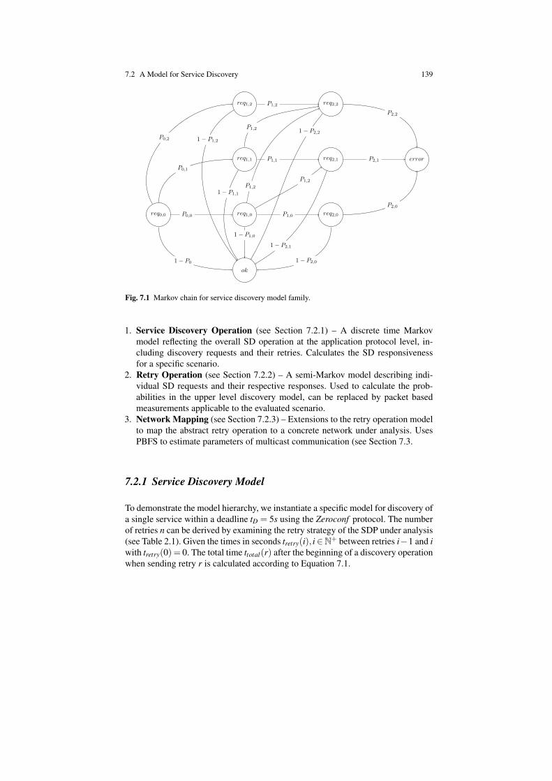
7.2 A Model for Service Discovery 139
req1,2 req2,2
req1,1 req2,1 error
req0,0 req1,0 req2,0
ok
P0,0
P0,1
P0,2
P1,0
P1,2P1,2
P1,1
P1,2
P1,2
P2,0
P2,1
P2,2
1− P0
1− P1,0
1− P1,1
1− P1,2
1− P2,0
1− P2,1
1− P2,2
Fig. 7.1 Markov chain for service discovery model family.
1. Service Discovery Operation (see Section 7.2.1) – A discrete time Markovmodel reflecting the overall SD operation at the application protocol level, in-cluding discovery requests and their retries. Calculates the SD responsivenessfor a specific scenario.
2. Retry Operation (see Section 7.2.2) – A semi-Markov model describing indi-vidual SD requests and their respective responses. Used to calculate the prob-abilities in the upper level discovery model, can be replaced by packet basedmeasurements applicable to the evaluated scenario.
3. Network Mapping (see Section 7.2.3) – Extensions to the retry operation modelto map the abstract retry operation to a concrete network under analysis. UsesPBFS to estimate parameters of multicast communication (see Section 7.3.
7.2.1 Service Discovery Model
To demonstrate the model hierarchy, we instantiate a specific model for discovery ofa single service within a deadline tD = 5s using the Zeroconf protocol. The numberof retries n can be derived by examining the retry strategy of the SDP under analysis(see Table 2.1). Given the times in seconds tretry(i), i∈N+ between retries i−1 and iwith tretry(0) = 0. The total time ttotal(r) after the beginning of a discovery operationwhen sending retry r is calculated according to Equation 7.1.
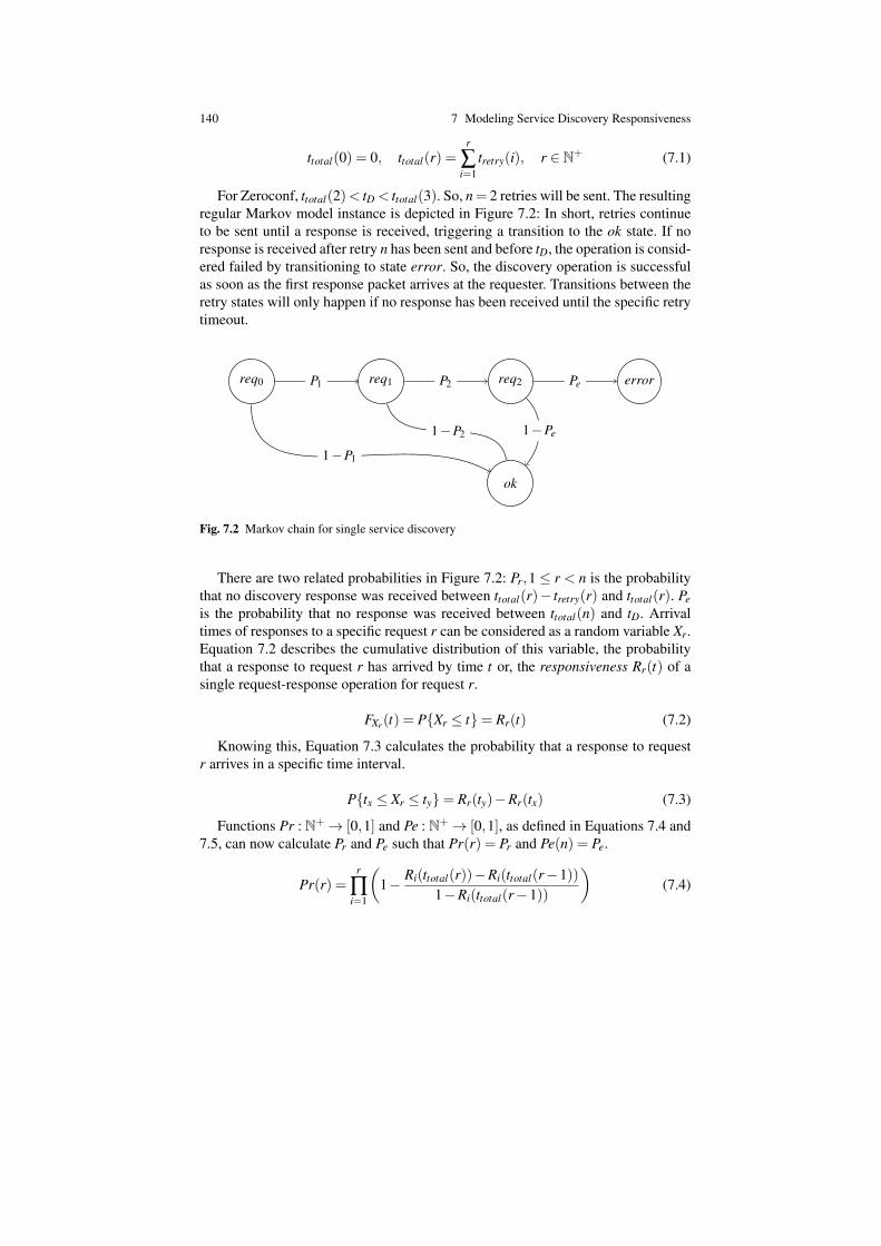
140 7 Modeling Service Discovery Responsiveness
ttotal(0) = 0, ttotal(r) =r
∑i=1
tretry(i), r ∈ N+ (7.1)
For Zeroconf, ttotal(2)< tD < ttotal(3). So, n= 2 retries will be sent. The resultingregular Markov model instance is depicted in Figure 7.2: In short, retries continueto be sent until a response is received, triggering a transition to the ok state. If noresponse is received after retry n has been sent and before tD, the operation is consid-ered failed by transitioning to state error. So, the discovery operation is successfulas soon as the first response packet arrives at the requester. Transitions between theretry states will only happen if no response has been received until the specific retrytimeout.
req0 req1 req2 error
ok
P1 P2 Pe
1−P1
1−P2 1−Pe
Fig. 7.2 Markov chain for single service discovery
There are two related probabilities in Figure 7.2: Pr,1 ≤ r < n is the probabilitythat no discovery response was received between ttotal(r)− tretry(r) and ttotal(r). Peis the probability that no response was received between ttotal(n) and tD. Arrivaltimes of responses to a specific request r can be considered as a random variable Xr.Equation 7.2 describes the cumulative distribution of this variable, the probabilitythat a response to request r has arrived by time t or, the responsiveness Rr(t) of asingle request-response operation for request r.
FXr(t) = P{Xr ≤ t}= Rr(t) (7.2)
Knowing this, Equation 7.3 calculates the probability that a response to requestr arrives in a specific time interval.
P{tx ≤ Xr ≤ ty}= Rr(ty)−Rr(tx) (7.3)
Functions Pr : N+→ [0,1] and Pe : N+→ [0,1], as defined in Equations 7.4 and7.5, can now calculate Pr and Pe such that Pr(r) = Pr and Pe(n) = Pe.
Pr(r) =r
∏i=1
1− Ri(ttotal(r))−Ri(ttotal(r−1))
1−Ri(ttotal(r−1))
(7.4)
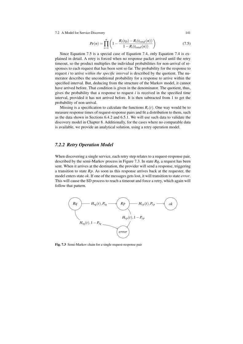
7.2 A Model for Service Discovery 141
Pe(n) =n
∏i=1
1− Ri(tD)−Ri(ttotal(n))
1−Ri(ttotal(n))
(7.5)
Since Equation 7.5 is a special case of Equation 7.4, only Equation 7.4 is ex-plained in detail. A retry is forced when no response packet arrived until the retrytimeout, so the product multiplies the individual probabilities for non-arrival of re-sponses to each request that has been sent so far. The probability for the response torequest i to arrive within the specific interval is described by the quotient. The nu-merator describes the unconditional probability for a response to arrive within thespecified interval. But, deducing from the structure of the Markov model, it cannothave arrived before. That condition is given in the denominator. The quotient, thus,gives the probability that a response to request i is received in the specified timeinterval, provided it has not arrived before. It is then subtracted from 1 to get theprobability of non-arrival.
Missing is a specification to calculate the functions Rr(t). One way would be tomeasure response times of request-response pairs and fit a distribution to them, suchas the data shown in Sections 6.4.2 and 6.5.1. We will use such data to validate thediscovery model in Chapter 8. Additionally, for the cases where no comparable datais available, we provide an analytical solution, using a retry operation model.
7.2.2 Retry Operation Model
When discovering a single service, each retry step relates to a request-response pair,described by the semi-Markov process in Figure 7.3. In state Rq, a request has beensent. When it arrives at the destination, the provider will send a response, triggeringa transition to state Rp. As soon as this response arrives back at the requester, themodel enters state ok. If one of the messages gets lost, it will transition to state error.This will cause the SD process to reach a timeout and force a retry, which again willfollow that pattern.
Rq Rp ok
error
Hrq(t),Prq Hrp(t),Prp
Hrq(t),1−Prq
Hrp(t),1−Prp
Fig. 7.3 Semi-Markov chain for a single request-response pair

142 7 Modeling Service Discovery Responsiveness
In case messages arrive (with a probability of Px), they have a certain distribu-tion of arrival times. This is described by Hx(t), the sojourn time distribution forstate x. The cumulative distribution function of time to absorption in state ok nowcalculates Rr(t) as in Equation 7.2. Since t is relative to the beginning of the SDoperation, Rr(t) is in fact parametrized by the location ttotal(r), the time at whichretry r is being initiated. The retry operation model is independent of a concrete net-work infrastructure. It has no knowledge of how to calculate the probabilities andtransition time distributions. Providing concrete values of Px and Hx(t) for specificSD pairs on demand is the purpose of the network mapping model.
7.2.3 Network Mapping Model
Mapping requests and responses to the network under analysis means providingmodels that calculate Px and Hx(t) in the retry operation model (see Figure 7.3) bytaking into account the details of the used communication mechanism, unicast ormulticast. This mapping is dependent on the concrete network infrastructure. In thiscase, we provide models for a WMN running OLSR [57]. Different networks couldneed diverse models, but, provided they estimate Px and Hx(t), these could be usedin the proposed model hierarchy as well.
Unicast Model
A unicast message follows the shortest path according to the routing metric. InOLSR, every node periodically calculates that shortest path and saves the next hopfor every destination. A unicast message is sent to the next hop node which thendecides to forward according to its own next hop information for the destination.We use an algorithm that calculates the unicast path hop by hop based on the nexthop information on each node. If no such global information is available, using theshortest path known to the first node remains a viable, albeit less accurate solution.
Since there is only one path with n nodes and m= n−1 links, this can be modeledas a simple semi-Markov chain of n states. Each state ki, i = 1...n− 1 stands for“message forwarded by node i”, state kn means “message arrived at node n”. Thelinks between nodes i and i+ 1 become transitions ki → ki+1. Further, there is atransition from ki, i = 1...n− 1 to error to account for packet loss. State transitionprobabilities Pki,ki+1 are calculated from the currently monitored packet transmissionprobabilities of the link between nodes i and i+ 1 (see Section 7.5), taking intoaccount that unicasts will be retransmitted up to seven times if not acknowledgedby the receiving node. The estimation of sojourn time distributions Hki,ki+1(t) isdescribed in Section 7.2.4. The resulting unicast chain is then integrated into theretry operation model in Figure 7.3 – for a unicast response, for example, by mergingstates ki and Rp, kn and ok as well as the two error states. The rest of the chainreplaces transition Rp→ ok.

7.2 A Model for Service Discovery 143
Multicast Model
In theory, modeling the traversal of a multicast discovery packet should consider allpossible paths between source and destination. Multicasts are in essence Network-Wide Broadcasts (NWBs) on a subgraph of the complete network, which containsall nodes taking part in the service network. This redundancy has been taken intoaccount in the methodology for service availability evaluation in Part II but findingall paths between two nodes is NP-complete, a prohibitive complexity in networkswith high connectivity, such as WMNs. Since the vast majority of those paths has avery low probability of traversal and their impact on the responsiveness of the multi-cast communication would be minor, this work instead proposes a different methodto estimate the reachability of multicast communication. Probabilistic Breadth-FirstSearch (PBFS) is a Monte Carlo method to derive an estimation of the multicast pathlength between given nodes that communicate using flooding or variations thereof.Because of its extensive use when estimating multicast communication within theSD models, PBFS needs a detailed description, which can be found in Section 7.3.
In PBFS, node neighbors are only considered if the edge between a node and itsneighbor succeeds a random roll against its transmission probability, as monitoredby the routing layer (see Section 7.5). This way, each run of PBFS realisticallysimulates how a multicast packet would traverse the WMN. PBFS is sampled asufficient number of times to approximate with which probability the destinationnode could be reached. This reflects Px in the retry operation model, for example,Prq for a multicast request. We additionally store the probability for each path lengthin case of arrival to later estimate the distribution of sojourn time Hx(t) in Section7.2.4.
7.2.4 Transmission Time Distributions
Estimations for sojourn time distributions in the network mapping models are basedon the (re-)transmission and potential back-off periods defined in the 802.11 stan-dard [120]. For transmission times over links, we assume the lowest data rate, whichis correct for multicasts. Unicasts, however, will transmit at higher data rates ifpossible, reducing the time for individual retry transmissions. The estimation thuspresents an upper bound for the transmission time as dependent on the data rate.The estimation also ignores additional contention due to internal traffic or externalinterference, which affects the upper limit of transmission times. To account for this,a certain percentage of packets is assumed to arrive after the estimated maximumtransmission time for both uni- and multicasts. The bounds calculated from these as-sumptions are fitted to an exponential distribution for the transmission time. For theunicast model, this is done for each transition ki→ ki+1, i = 1...n− 1 and providesHki,ki+1(t). In the multicast model, one distribution function is generated for eachpossible path length given by PBFS. The distributions are then weighted with thecorresponding probability for their length and combined in a single function Hx(t).

144 7 Modeling Service Discovery Responsiveness
7.3 Multicast Reachability Estimation
As previously described in Section 2.2.2, all SDPs use multicast communicationfor crucial parts of the discovery process. However, due to the characteristics ofwireless communication, NWBs are generally problematic in WMNs. Being able toestimate NWB dissemination in such networks is thus fundamental when estimatingpacket traversal probabilities and traversal times, as needed for the lower-level mod-els in Sections 7.2.3 and 7.2.4. Most existing dissemination models neglect the realnature of WMNs and are based on simple graph models, which provide optimisticassumptions of NWB dissemination. On the other hand, models that fully considerthe complex propagation characteristics of NWBs quickly become unsolvable dueto their complexity.
In this section, we present the details of the Monte Carlo method PBFS to approx-imate the reachability of NWB protocols. PBFS has been described in more detailin [11]. Without reverting to expensive empirical or analytical methods, PBFS canbe used to realistically approximate various metrics, such as reachability or averagepath length. PBFS simulates individual NWBs on graphs with probabilistic edgeweights, which reflect link qualities of individual wireless links in the WMN, andestimates reachability over a configurable number of simulated runs. This approachnot only has a very low time and space complexity compared to existing approaches,but further provides additional information, such as the distribution of path lengths.Furthermore, it is easily extensible to NWB schemes other than flooding. The appli-cability of PBFS is validated both theoretically and empirically in Section 7.4.
7.3.1 Network Model
A WMN can be modeled as an undirected graph G=(V,E), where each vertex v∈Vcorresponds to a WMN node and each edge e ∈ E corresponds to a wireless com-munication link between two nodes. In Quasi Unit Disk Graphs (QUDGs) [132],there is a communication link between two nodes if their Euclidian distance is lessthan d (with 0 < d < 1) and none if it is greater, otherwise unspecified. Thus, a linkmay or may not exist within this uncertainty range. This neglects that links itself arerarely perfect or completely non-existent, but their quality varies in between. Forexample, there might be good links which succeed in transmitting packets 85% ofthe time, while others succeed only 10% of the time. Thus, in the model proposed inthis section wireless links are not just binary but approximated with a transmissionprobability pi, j, the probability a transmission from node i to node j succeeds (seeEquation 7.6). If pi, j = 0, the edge is not included in the graph.
pi, j : E→ [0,1] (7.6)
In practice, pi, j usually reflects a measurement-based approximation. Link qual-ities are never constant but vary over time due to small-scale fading effects, micro-

7.3 Multicast Reachability Estimation 145
mobility of the environment and interference. Node outages may also happen. Thegraph model assumes independence between the qualities of different links, any de-pendence is expected to be already included in the approximation of pi, j. For theapplication in the context of this work, SD in WMNs (see case study in Section7.6), static networks with no node mobility are assumed. However, the method de-scribed in Section 7.3.4 can also be adjusted to support network topology dynamicsreflected in varying values for pi, j.
7.3.2 Reachability Metrics for Network-wide Broadcasts
To evaluate the performance of NWBs within the weighted graph model, we definereachability as the main metric, which captures an important aspect of the depend-ability of a NWB. We distinguish between the following two reachabilities:
Individual reachability ra→b – The probability that a node b is reached by aNWB initiated by node a. In practice, ra→b is averaged over multiple runs asa single run will only give a binary value.
Global reachability ra – The percentage of nodes that receives a NWB sent bynode a. Let R be the number of nodes reached by a NWB initiated from nodea. The global reachability is defined as ra =
R|V | and derived from a single NWB
or averaged over multiple NWBs. For a general statement about the performanceof a protocol or a given topology this should be averaged over a large numberof runs. Another way to derive the global reachability would be to average allindividual reachabilities.
Global and individual reachabilities depend on the given network topology withits transmission probabilities, NWB protocol, NWB source node and, for individualreachability, the destination node. Source independent results can be achieved byconsidering NWBs from every node in the network and averaging over all of them.
7.3.3 Calculation of Reachability
There exist purely analytical methods to calculate the reachability metrics based onthe described weighted graph model. For example, Chen et al. [50] have shown howthe individual reachability ra→b can be obtained by summing up the probabilities ofthe family of edge sets that contain a path from a to b, as in Equation 7.7: 2E
a→b is theset of all subsets of edges that contain a path from a to b. Calculating this formulahas an exponential complexity due to the iteration of the power set.
ra→b = ∑E ′∈2E
a→b
∏
(i, j)∈E ′pi, j ∏
(k,l)∈E\E ′(1− pk,l)
(7.7)

146 7 Modeling Service Discovery Responsiveness
Another possible approach is to enumerate all given paths between a and b andcalculate the probability of not reaching node b over any of these paths. Enumeratingall simple paths between two nodes is NP-hard for arbitrary graphs. Furthermore,as these paths are not independent and can contain common subpaths, this approachrequires factoring out these common subpaths, which is again NP-hard, a prohibitivecomplexity in highly connected WMNs. However, for certain networks with a lowconnectivity, hence, a low in-degree of the nodes, this approach is viable and weare taking it into account in Part II when presenting an approach to automaticallygenerate user-perceived service availability models.
Chen’s algorithm for the Flooding Path Probability (FPP) [50] also computes theindividual reachability ra→b. It resorts to computing the joint probability distributionthat a packet is received by a subset of the vertex cut in each step of its algorithm.The complexity is O(N(C∆+ + 2C∆−)), where C is the size of the largest vertexcut used by the algorithm, ∆+ is the maximum out-degree and ∆− the maximumin-degree of the graph. Therefore, calculating the FPP is efficient if the network hasonly a small largest vertex cut, which is not true for high connectivity WMNs.
Given their complexity, these existing approaches are only feasible in simplenetworks. To support the reachability evaluation of NWBs as used by discoveryprotocols in WMNs, a more efficient method is needed. Equation 7.7 will be used inSection 7.4.1, however, to validate the proposed PBFS in exemplary small networks.
7.3.4 Probabilistic Breadth-First Search
We will now introduce the Monte Carlo method Probabilistic Breadth-First Search(PBFS) that models flooding as a slight modification of Breadth-First Search (BFS)[87] in a weighted graph as described in Section 7.3.1. In contrast to regular BFS,in PBFS, for a node i its neighbor j in the graph is only considered if the edgebetween i and j succeeds a random roll against its transmission probability pi, j.Consequently, PBFS can be seen as a flooding process in a graph whose edges areweighted with independent transmission probabilities, abstracting from wireless ef-fects such as contention and collisions. This way, each run of PBFS simulates howa NWB packet, for example a discovery request, would traverse the WMN. It doesso without resorting to complex network simulations or testbed experiments as inChapter 6, and with considerably lower complexity than the purely analytical eval-uations in Section 7.3.3. The algorithm has previously been published in [11] and ispresented in Figure 7.4.
The global reachability rsrc is ratio of the number of nodes that were marked(reached) to the number of all nodes. In real networks, for example, the probabilis-tic edge weights pi, j in the graph can be obtained by doing link probing for the ETXmetric as described in Section 7.5. The PBFS procedure in Figure 7.4 samples a suf-ficient number of times to approximate with which probability a destination node bis reached by a NWB from node a (the individual reachability ra→b). This reflectsPx in the retry operation model from Section 7.2.2, for example, Prq for a multicast

7.3 Multicast Reachability Estimation 147
1: procedure PBFS(G, src) ▷ G provides nodes and pi, j .2: mark[n]← False ∀ n ∈ G ▷ BFS visited marker.3: NoT[n]← 1 ∀ n ∈ G ▷ Number of transmissions setup.4: reached← 0 ▷ How many nodes were finally reached.5: nodes← [src] ▷ Queue of nodes to be processed.6: mark[src]← True7: while nodes =∅ do8: i← nodes.dequeue()9: for j ∈ G.neighbors(i) do
10: psuccess ← 1− (1− pi, j)NoT [i]
11: if mark[j] = False ∧ random() < psuccess then12: nodes.enqueue(j)13: mark[j]← True14: reached← reached + 115: end if16: end for17: end while18: end procedure
Fig. 7.4 Demonstration of the basic Probabilistic Breadth-First Search (PBFS) algorithm, whichmimics flooding in a WMN.
request. Additionally, PBFS approximates over how many hops b is reached, pro-viding a list of tuples with the probability for any path length b is reachable by theflooding process initiated by a. This list can be used to estimate the transmissiontime distribution functions Hx(t) in the retry operation model as described in Sec-tion 7.2.4. For reasons of brevity, path length distributions have not been included inFigure 7.4. It should be mentioned that while throughout this work, only undirectedgraphs are considered, PBFS can be used just as well on directed graphs.
PBFS has several advantages over the existing analytical approaches. First, it iscomputationally less complex as the FPP [50] resorts to computing the joint prob-ability distribution that a packet is received by a subset of the vertex cut in eachstep of its algorithm. PBFS instead has the complexity O(|E|+ |V |) of BFS [60],which allows to calculate reachability even for large graphs. PBFS also providesover how many hops a node is reached and with which probability. Furthermore,it does that not only for one node pair but for all reachable nodes from a specificNWB source node. PBFS can work with dynamic values of pi, j. Provided a functionthat calculates pi, j over time or a series of ETX measurements, each run of PBFScould use different values for pi, j as input. Additionally, it is possible to modifyPBFS to model modifications of basic flooding and other NWB approaches, as hasbeen demonstrated in [11]. For example, PBFS allows for different configurationsof transmissions done by each node (see code in Figure 7.4, Lines 3 and 10).

148 7 Modeling Service Discovery Responsiveness
7.4 Multicast Reachability Validation
As PBFS relies on repeated randomized sampling runs, it reflects a Monte-Carlomethod to approximate reachability. In a nutshell, more runs increase the accuracyof its approximation. An estimation of a sufficient sampling number for PBFS, itsdeviation from the exact theoretical reachability and its confidence follows in Sec-tions 7.4.1 and 7.4.2.
7.4.1 Theoretical Validation
For theoretical validation, PBFS is evaluated in three exemplary small networks,where the complexity still allows a precise analytic assessment of reachability usingEquation 7.7. These networks are depicted in Figure 7.5. All three network graphsare depicted within one Figure. The first network G1 consists of nodes a, b, c andd and connecting links. The second G2 adds nodes e and f to G1, while the thirdnetwork G3 consists of the whole graph in Figure 7.5. Edge labels correspond topi, j.
0.6 0.5
0.7
0.4
0.5
0.4
0.3
0.7
0.9
0.8
0.6
0.6
0.4
0.3
0.2
0.3
a
c
b
e
dg
f
i
h
G1 G2 G3
Fig. 7.5 Three example networks for theoretical validation: {a,b,c,d}, {a,b,c,d,e, f} and{a,b,c,d,e, f ,g,h, i} including all links connecting the nodes. [11]
Evaluation results are listed in Table 7.1. It lists the values of three differentreachabilities when calculated using Equation 7.7 and when approximated by PBFS

7.4 Multicast Reachability Validation 149
over a certain number of runs x. The run-time of the algorithms is included in paren-theses as a reference. The results demonstrate two phenomena: First, the exponentialincrease in runtime when using Equation 7.7 is visible already for these simple net-works. Since execution times are based on non-optimized implementations, theyhave to be taken with a grain of salt. But the effect of combinatorial explosion usingEquation 7.7 is obvious. Second, one can see that PBFS converges relatively fastto the correct reachability value. Already after only 1000 runs, the relative error isaround 5% and below 0.5% after 100000 runs with a confidence of 99%.
Table 7.1 PBFS deviation (with 99% confidence after 1000 trials) with different number of runsx, implementation runtime included in parentheses for illustration.
Network Nodes / Edges Reachability Equation 7.7 PBFS PBFS PBFSevaluated x1 = 103 x2 = 104 x3 = 105
G1 4 / 5 ra→d 0.22824 ±5.10% ±1.58% ±0.47%(0.004 s) (0.020 s) (0.199 s) (1.990 s)
G2 6 / 9 ra→ f 0.19682 ±4.71% ±1.45% ±0.48%(0.116 s) (0.023 s) (0.230 s) (2.275 s)
G3 9 / 16 ra→i 0.39104 ±6.30% ±1.90% ±0.59%(31.004 s) (0.032 s) (0.315 s) (3.179 s)
The standard deviation of a Monte Carlo method is determined as in Equation7.8. Here, the value of x represents the number of iterations in PBFS while e is theabsolute error.
σ =√
x · e (7.8)
Given the characteristics of PBFS, we have to assume a constant standard devi-ation of the calculated reachabilities. This means that the absolute error decreaseswith an increasing number of runs while the standard deviation remains the same(see Equation 7.9).
σ =√
x1 · e1 =√
x2 · e2 = · · ·=√
xn · en (7.9)
So with an increasing number of runs we see the error decreasing by a factor asin Equation 7.10
en
em=
xm
xn,m > n (7.10)
In fact, this expected behavior is reflected by a linear decrease of the absoluteerror in the logarithmic plot in Figure 7.6. Together with the convergence of reacha-bility it validates PBFS as a proper Monte Carlo method to approximate the behaviorof NWBs.

150 7 Modeling Service Discovery Responsiveness
100 101 102 103 104 105
Number of PBFS runs
10−3
10−2
10−1
100
Abs
olut
eer
ror
Fig. 7.6 Absolute PBFS error (y-axis) over number of runs (x-axis). Obtained by comparing PBFSresults with Equation 7.7 for network G3 in Figure 7.5. Axes have a logarithmic scale. [11]
7.4.2 Experimental Validation
To justify the feasibility of PBFS when reproducing properties of real world WMNs,this section provides an experimental validation. We compare the global and individ-ual reachability approximations given by PBFS with results measured in simulationsand a wireless testbed. We focus on basic flooding as NWB across different networktopologies because it is the main method used to date and as such the basis of themulticast model in Section 7.2.3. Furthermore, hop length distributions for exem-plary node pairs are shown and compared, which are needed for the calculation oftransmission time distributions as in Section 7.2.4. PBFS estimations are expectedto have a higher deviation, as it abstracts from short-term effects not reflected in themeasured transition probabilities pi, j.
Experiment Setup
Flooding is implemented within the Click Modular Router framework [130], whichallows to run it either in a wireless testbed or in simulators. For real-word experi-ments, the DES-Testbed at Freie Universitat Berlin is used as it was the case alreadyin Chapter 6. This testbed consists of around 130 wireless nodes equipped with IEEE802.11 hardware that are spread over multiple campus buildings of FUB. We referto [36] for a complete description of the testbed. As simulator, ns-3.14 [115, 13]with extensions for Click is employed. The wireless model is based on the Jakespropagation loss model [248], nodes form an NPART topology [160] consisting of275 nodes. Different scenarios are obtained by varying the transmission power in thetestbed as well as in simulations. Measuring transmission probabilities pi, j, whichare the input to PBFS, is done by a link prober that sends neighbor discovery pack-ets and calculates the ETX [62]. Flooding packets are sent as link-layer broadcastswith a fixed 1 Mbps data rate and payload sizes of 400 bytes, the same size as theprobing packets. In each scenario one node was chosen to start 1000 NWBs. The

7.4 Multicast Reachability Validation 151
achieved global and individual reachabilities are then evaluated and compared withthe ones obtained by running PBFS using the same pi, j from the link prober.
Experiment Results
In Figure 7.7, the global reachability for flooding is shown, contrasting results ob-tained by PBFS with measurements from the testbed and simulation (Figures 7.7aand 7.7b, respectively). One data point corresponds to the reachability in a singlescenario. Linear regression results in the dashed line and shows a very strong linearcorrelation with a correlation coefficient r greater than 0.99 and very small p-valuesin both comparisons. This indicates a strong presumption against the null hypothe-sis, meaning that there is no relationship between the two data sets. The completeresults of the linear regression are listed in Table 7.2. PBFS slightly over-estimatesreachability when compared to simulations, an effect that is not shown in testbedresults. This bias in simulations hints at a systemic property in the simulation setupthat needs further investigation.
0.0 0.2 0.4 0.6 0.8 1.0Global reachability (Testbed)
0.0
0.2
0.4
0.6
0.8
1.0
Glo
balr
each
abili
ty(P
BFS)
(a) PBFS vs. Testbed
0.0 0.2 0.4 0.6 0.8 1.0Global reachability (Simulation)
0.0
0.2
0.4
0.6
0.8
1.0
Glo
balr
each
abili
ty(P
BFS)
(b) PBFS vs. Simulation
Fig. 7.7 Comparison of global reachability predicted by PBFS (y-axis) versus achieved in realityand by simulation (x-axis). A point constitutes the reachability for a single scenario [11].
Figure 7.8 shows the individual node reachabilities (top graphs) with their cor-responding empirical cumulative distribution functions of the absolute differencebetween predicted and achieved reachabilities for all nodes (bottom graphs). Again,a data point reflects the reachability of a single node as estimated by PBFS versusthe results from testbed or simulation. The shaded area in the top graphs constitutesan absolute error±10% of the ideal line with slope 1. Linear regression with all datapoints results in the solid line.

152 7 Modeling Service Discovery Responsiveness
Table 7.2 Values of the linear regression when correlating PBFS with experiment results. Theregression line is of the form Y = a+b ·X .
Experiment slope b intercept a r-value p-value standard error
PBFS vs. Testbed 1.015 −0.043 0.99 2.038 ·10−13 0.038PBFS vs. Simulation 1.116 0.013 0.995 2.578 ·10−7 0.044
0.0 0.2 0.4 0.6 0.8 1.0Invididual reachability (Testbed)
0.0
0.2
0.4
0.6
0.8
1.0
Indi
vidu
alre
acha
bilit
y(P
BFS)
0.0 0.2 0.4 0.6 0.8 1.0Invididual reachability (Simulation)
0.0
0.2
0.4
0.6
0.8
1.0
Indi
vidu
alre
acha
bilit
y(P
BFS)
0.0 0.2 0.4 0.6 0.8 1.0Absolute error (Testbed vs PBFS)
0.0
0.2
0.4
0.6
0.8
1.0
Empi
rica
lCD
F
0.0 0.2 0.4 0.6 0.8 1.0Absolute error (Simulation vs PBFS)
0.0
0.2
0.4
0.6
0.8
1.0
Empi
rica
lCD
F
Fig. 7.8 Comparison of individual node reachabilities predicted by PBFS (y-axis) and achievedin reality or simulations (x-axis) across different scenarios (top). Corresponding CDF plots for theabsolute differences shown in the bottom graphs. [11]
While there are outliers when compared with both simulation and testbed re-sults, PBFS reasonably approximates the measured reachability. Simulation showsa much narrower distribution, although the points show a characteristic curve whichagain hints at some systematic property of the simulation model that warrants fur-ther research. Investigating this, however, is out of the scope of this work. In thebottom graphs, the corresponding CDF plots for the absolute differences are shown.The CDF plots show that in both setups, the PBFS approximation does not differmore than 0.2 from the measured reachability for 80% of all data points.
Last but not least, PBFS provides the distribution of path length probabilities foreach destination node of a NWB as needed for the transmission time estimationsin Section 7.2.4. A comparison of these distributions between PBFS and testbed
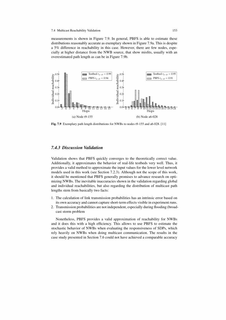
7.4 Multicast Reachability Validation 153
measurements is shown in Figure 7.9. In general, PBFS is able to estimate thesedistributions reasonably accurate as exemplary shown in Figure 7.9a. This is despitea 5% difference in reachability in this case. However, there are few nodes, espe-cially at higher distance from the NWB source, that show misfits, usually with anoverestimated path length as can be in Figure 7.9b.
3 4 5 6 7 8 9 10 11 12 13 14 15Hops
0.0
0.1
0.2
0.3
0.4
0.5
Indi
vidu
alre
acha
bilit
y Testbed ra→b = 0.99
PBFS ra→b = 0.94
(a) Node t9-155
4 5 6 7 8 9 10 11 12 13 14 15 16 17 18 19 24Hops
0.0
0.1
0.2
0.3
0.4
0.5
Indi
vidu
alre
acha
bilit
y Testbed ra→b = 0.95
PBFS ra→b = 0.91
(b) Node a6-028
Fig. 7.9 Exemplary path length distributions for NWBs to nodes t9-155 and a6-028. [11]
7.4.3 Discussion Validation
Validation shows that PBFS quickly converges to the theoretically correct value.Additionally, it approximates the behavior of real-life testbeds very well. Thus, itprovides a valid method to approximate the input values for the lower level networkmodels used in this work (see Section 7.2.3). Although not the scope of this work,it should be mentioned that PBFS generally promises to advance research on opti-mizing NWBs. The inevitable inaccuracies shown in the validation regarding globaland individual reachabilities, but also regarding the distribution of multicast pathlengths stem from basically two facts:
1. The calculation of link transmission probabilities has an intrinsic error based onits own accuracy and cannot capture short-term effects visible in experiment runs.
2. Transmission probabilities are not independent, especially during flooding (broad-cast storm problem
Nonetheless, PBFS provides a valid approximation of reachability for NWBsand it does this with a high efficiency. This allows to use PBFS to estimate thestochastic behavior of NWBs when evaluating the responsiveness of SDPs, whichrely heavily on NWBs when doing multicast communication. The results in thecase study presented in Section 7.6 could not have achieved a comparable accuracy

154 7 Modeling Service Discovery Responsiveness
without resorting to considerably more complex methods. In fact, the complexity ofthose models would have prohibited similar analysis.
7.5 Model Generation and Solution
After describing the various layers of the stochastic model hierarchy and the meth-ods to measure or calculate their input parameters, it is now time to put the modelsinto use. So, to calculate the SD responsiveness for given pairs of requester andprovider in a network, the model layers described in Sections 7.2 need to be gener-ated bottom-up using the following steps:
1. Define a scenario which consists of (1) the SD communication partners requesterand provider, (2) the discovery protocol and (3) a deadline for the SD operation.
2. Generate low level network mapping models for individual requests and re-sponses between the SD pair requester and provider based on the communica-tion mechanisms of the protocol, uni- or multicast (see Sections 7.2.3, 7.2.4 and7.3.4).
3. Integrate the network mapping models from Step 2 in the semi-Markov chain forthe retry model (see Section 7.2.2). This chain calculates the responsiveness ofan individual retry over time.
4. Calculate the number of retries n based on the defined protocol and deadline.This defines the structure of the high level discovery model (see Section 7.2.1).
5. Estimate the state transitions probabilities in the discovery model, using Equa-tions 7.4 and 7.5. In these equations, Rn(t) is the cumulative probability for ab-sorption at time t in state ok in the retry model from Step 3.
The discovery model can then be solved. The steady-state probability of arrivalin state ok in this model is the probability that an SD operation as specified in thescenario is successful, given the current monitored state of the network. The method-ology has been implemented in a Python [191] framework that carries out all neces-sary steps. More complex stochastic analysis is performed using the SHARPE tool[224].
Monitoring
All monitoring data is gathered on demand from the routing layer. This approachis least invasive and can be used in every network where the routing layer providesthe needed data. OLSR nodes use probe messages to measure link qualities for ev-ery neighbor. Given the forward delivery ratio d f and reverse delivery ratio dr, theExpected Transmission Count (ETX) [62] is defined as in Equation 7.11. This infor-mation allows to construct a complete network graph with edges weighted by theirETX value. In the graph, nodes are annotated with meta information from their local

7.6 Case Study 155
OLSR routing table that includes the next hop for every other reachable node in thenetwork.
ETX =1
(d f ·dr)(7.11)
7.6 Case Study
To demonstrate how the proposed methodology can be used to estimate the respon-siveness in common use cases of SD, three of the protocols explained in Section2.2.2 – Zeroconf , Simple Service Discovery Protocol SSDP and Service LocationProtocol SLP – are now evaluated in three different scenarios using measured datafrom a real-life WMN, the Distributed Embedded Systems (DES) testbed at FreieUniversitat Berlin (FUB). For the sake of traceability, node identifiers in this textreflect the actual hostnames in the testbed. Due to space limitations, we refer to acomplete description of the testbed in [36].
In this case study, OLSR [57] was used in version 0.6.5.2. It provides a validreference for the real world application of the methodology. All monitoring wasdone by OLSR. Topology data was gathered with OLSR’s JavaScript Object Nota-tion (JSON) plug-in and then integrated into the network model using the Pythonframework. The testbed was configured and data gathered with different transmis-sion power levels to obtain different topologies. Retry intervals of the SDPs are setaccording to the standards as described in Section 2.2.2 and Table 2.1. Since SSDPdoes not have fixed intervals, it is assessed in two different configurations reflectingthe minimum and maximum interval as defined in the standard.
7.6.1 Scenario 1 – Single Pair Responsiveness
First, the responsiveness of a single pair requester and provider is evaluated overtime. In order to investigate also how the responsiveness changes with the distancebetween nodes, two different pairs were chosen. One pair (t9-105, t9-154) is withinthe main cloud t9, a dense and well-connected part of the WMN consisting of 56nodes (see Figure 7.10a). The other pair (t9-105, a3-119) covers almost the max-imum distance in the network (see Figure 7.10b). In both cases, node t9-105 isthe requester. The results clearly show that as the distance between requester andprovider increases, overall responsiveness decreases.
The difference in responsiveness among the protocols is apparent. With increas-ing deadlines the responsiveness of the Zeroconf protocol is consistently lowercompared to the other protocols. This is because Zeroconf uses multicast for bothrequests and responses. Multicast packets will not be resent seven times before con-sidered lost, so the danger of packet loss is much higher. The positive effects of mul-

156 7 Modeling Service Discovery Responsiveness
0 5 10 15 20 25 30Time in seconds
0.2
0.4
0.6
0.8
1.0
Res
pons
iven
ess
ZCONFSLPSSDPminSSDPmax
(a) Within same cloud, provider t9-154
0 5 10 15 20 25 30Time in seconds
0.2
0.4
0.6
0.8
1.0
Res
pons
iven
ess
(b) Maximum distance, provider a3-119
Fig. 7.10 Discovery responsiveness over time for different providers requested from t9-105. [4]
ticast responses for multiple communication pairs, as pointed out in Section 2.2.1,cannot be considered in this analysis. Also not included are the effects of additionalload on the network caused by discovery. Since retries are considered independentevents, lower retry intervals will lead to a higher responsiveness. While this assump-tion can be justified for retry intervals in the order of seconds – discovery packetsare only a few bytes in size – it cannot hold for ever-lower intervals. So, althoughSSDP with a minimum interval ranks consistently best, the increased load mightnot be in the best interest of the service network as a whole. More in-depth researchis needed on that matter. However, it can be deducted that with low deadlines, thechosen retry interval is more relevant for responsiveness than the communicationmechanism (i.e., unicast vs. multicast). In general, current SDPs struggle to achievea high responsiveness in WMNs, even over short distances.
7.6.2 Scenario 2 – Average Provider Responsiveness
The second scenario covers the average responsiveness of a single provider overtime when requested from an arbitrary client in the network. To demonstrate how themodels capture topology changes, this scenario uses data measured in two differenttopologies that were generated with different radio power settings. The focus lies onprovider t9-154 from Section 7.6.1, which is well centered within the network so itprovides a good reference to see the effects of overall link quality on responsiveness.Figure 7.11 shows the results.
The main observation is that the average responsiveness when discovering nodet9-154 is quite high due to its prominent, almost optimal position in the network.With high quality radio links, depicted in Figure 7.11a, all protocols quickly reacha responsiveness of over 90%. Responsiveness is considerably decreased for lowerquality wireless connections (see Figure 7.11b). With deadlines above 15 seconds,

7.6 Case Study 157
0 5 10 15 20 25 30Time in seconds
0.2
0.4
0.6
0.8
1.0
Res
pons
iven
ess
ZCONFSLPSSDPminSSDPmax
(a) High radio power
0 5 10 15 20 25 30Time in seconds
0.2
0.4
0.6
0.8
1.0
Res
pons
iven
ess
(b) Low radio power
Fig. 7.11 Average responsiveness over time for provider t9-154 in different topologies. [4]
there is a consistent ranking of the SDPs, with Zeroconf again having the lowestresponsiveness. The ranking is identical for different link qualities, only the over-all values are different. Due to different retry strategies of the protocols, however,this behavior is not consistent for lower deadlines. This underlines the findings fromScenario 1: With deadlines close to the individual retry intervals, the chosen in-terval is more relevant for responsiveness than the communication mechanism. Insummary, it can be said that purely multicast based SD as in Zeroconf is justifiedwhen positive effects for multiple communication partners are expected. For singlediscovery operations among few partners, responding via unicast like in SSDP andSLP provides higher responsiveness because of its more reliable communicationmechanism. Among SSDP and SLP, the specific retry strategy until the deadline isthe main factor impacting responsiveness.
7.6.3 Scenario 3 – Expected Responsiveness Distance
The last scenario covers the expected responsiveness distance der from Definition1.4. The responsiveness of two different providers, t9-154 and a3-119, is calculatedwhen requested from every client in the network. Then, the responsiveness is av-eraged for requesters at the same distance of these providers. Again, the used datawas measured in two different topologies that were generated with different radiopower settings. The discovery deadline is set to five seconds. Results are illustratedin Figure 7.12.
The ranking among the protocols is not the same as in the previous scenarios.This is due to the chosen, realistically short deadline of five seconds. The retry strat-egy until this deadline has an important impact and the maximum retry timeout forSSDP simply did not force enough retries to account for lost messages. It can alsobe recognized in Figure 7.12d, that badly placed providers risk a very low der with
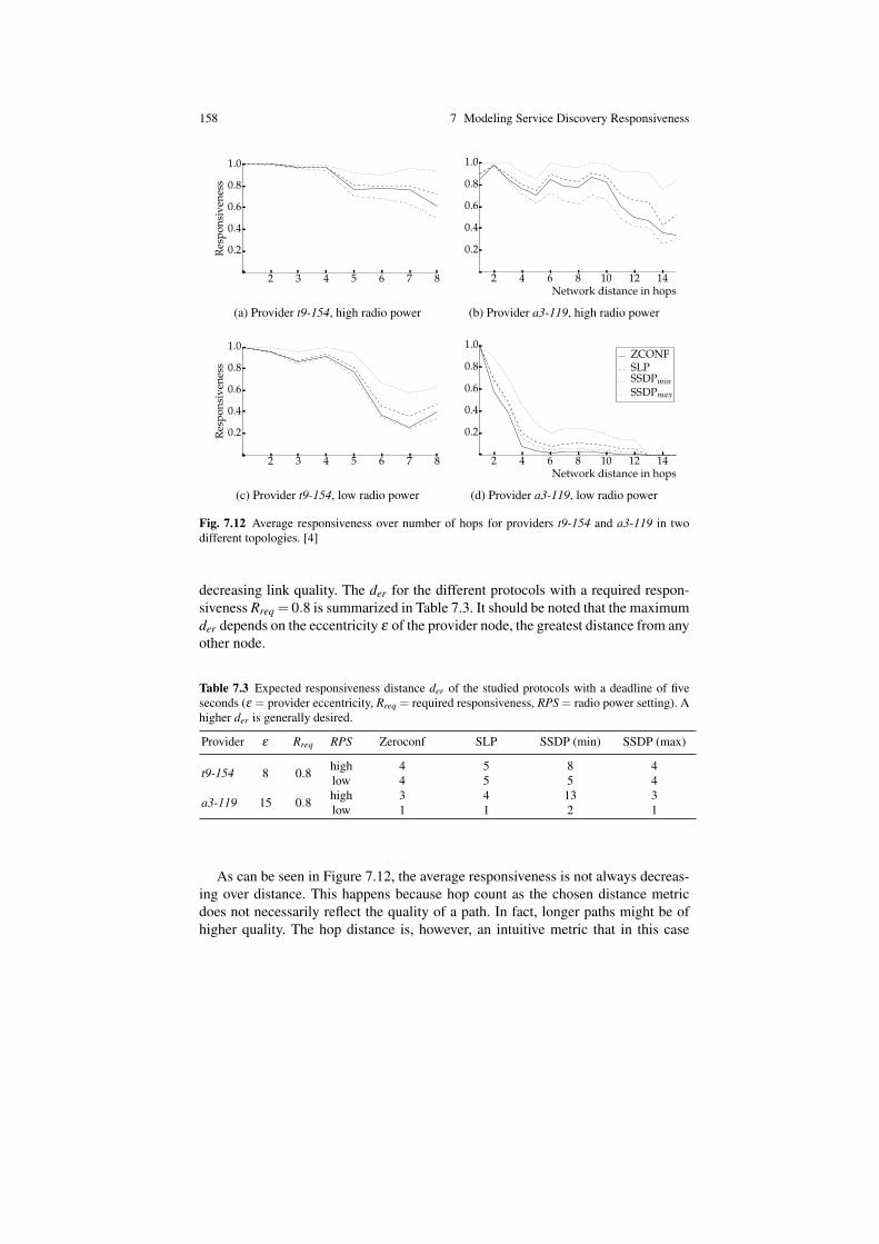
158 7 Modeling Service Discovery Responsiveness
2 3 4 5 6 7 8Network distance in hops
0.2
0.4
0.6
0.8
1.0
Res
pons
iven
ess
(a) Provider t9-154, high radio power
2 4 6 8 10 12 14Network distance in hops
0.2
0.4
0.6
0.8
1.0
Res
pons
iven
ess
(b) Provider a3-119, high radio power
2 3 4 5 6 7 8Network distance in hops
0.2
0.4
0.6
0.8
1.0
Res
pons
iven
ess
(c) Provider t9-154, low radio power
2 4 6 8 10 12 14Network distance in hops
0.2
0.4
0.6
0.8
1.0
Res
pons
iven
ess
ZCONFSLPSSDPminSSDPmax
(d) Provider a3-119, low radio power
Fig. 7.12 Average responsiveness over number of hops for providers t9-154 and a3-119 in twodifferent topologies. [4]
decreasing link quality. The der for the different protocols with a required respon-siveness Rreq = 0.8 is summarized in Table 7.3. It should be noted that the maximumder depends on the eccentricity ε of the provider node, the greatest distance from anyother node.
Table 7.3 Expected responsiveness distance der of the studied protocols with a deadline of fiveseconds (ε = provider eccentricity, Rreq = required responsiveness, RPS = radio power setting). Ahigher der is generally desired.
Provider ε Rreq RPS Zeroconf SLP SSDP (min) SSDP (max)
t9-154 8 0.8 high 4 5 8 4low 4 5 5 4
a3-119 15 0.8 high 3 4 13 3low 1 1 2 1
As can be seen in Figure 7.12, the average responsiveness is not always decreas-ing over distance. This happens because hop count as the chosen distance metricdoes not necessarily reflect the quality of a path. In fact, longer paths might be ofhigher quality. The hop distance is, however, an intuitive metric that in this case

7.7 Conclusion 159
presents the lower bound for der. If needed, a more realistic, quality-based distancemetric should be used to increase accuracy.
7.7 Conclusion
The case study on SD responsiveness as calculated by the presented models con-cludes this chapter. Results demonstrate that responsiveness varies dramatically de-pending on the position of nodes in the network and the overall link quality. Theresults further indicate that, with short deadlines close to the individual retry in-tervals, the right retry timing strategy is more important than the communicationmechanism. With longer deadlines, using the more reliable unicast instead of mul-ticast consistently improves responsiveness. In either case, the fixed strategies ofcurrent SD protocols struggle to achieve a high responsiveness in these dynamicand inherently unreliable networks. In Chapter 8, a comprehensive experimentalvalidation of the models is presented.


Chapter 8Correlating Model and Measurements
Abstract After demonstrating the Service Discovery (SD) responsiveness modelsin Chapter 7, the accuracy of the model estimations needs to be validated. This isdone by comparing the model results to results measured in experiments. Severalrepresentative scenarios for active single SD are chosen with varying fault intensity.Corresponding to previous experiments, the first set of scenarios covers SD behav-ior with increasing load. In the second set the radio signal power on the nodes isdecreased to reduce link quality. The empirical cumulative distribution functions ofthe SD response times in experiments, which reflect the responsiveness of SD arecompared to the model outputs based on low level network measurements taken dur-ing the same period. We show that wherever direct SD packet measurements can beused, the model output has a very low error. When monitoring data from the routinglayer is used, the error of the model has a consistently higher error depending on thequality of this input data.
8.1 Introduction
The focus of this chapter is the validation of the different layers of the model hier-archy which was introduced in Chapter 7. We use data gathered in experiments inthe DES testbed, which was in parts already presented in Chapter 6, and correlateestimations given by the model with actual measured data in corresponding exper-iments. In experiments, three types of data are being recorded that are useful whencorrelating model results: Events, packets and topology (see also Sections 3.4 and6.3.2).
Events The events reflect state changes in the Service Discovery (SD) process,such as “SD operation started” and “SD response received”. These time-stampedevents allow to calculate the responsiveness of SD operations on the applicationlayer, which should correlate to the steady-state probability of arrival in state okin the discovery model presented in Section 7.2.1.
161

162 8 Correlating Model and Measurements
Packets Events are caused by packet transmissions on the network communica-tion layer. A request initiated on the SD layer will cause a request packet to besent, with eventual retries until a sufficient number of responses has been re-ceived. Each of the arriving responses will in turn cause an event on the SDlayer. Since ExCovery adds unique identifiers to SD requests (see Section 3.7),each arriving response packet can be matched with the original request packet.The responsiveness of these pairs request and response can also be calculated. Itcorresponds to the cumulative probability for absorption in state ok in the retrymodel (see Section 7.2.2). As such, packet measurements can be used to validatethe discovery model isolated from the lower models in the hierarchy.
Topology In each run, a full snapshot of the topology is recorded as reflectedin the local views of each node. Every snapshot contains all known nodes, theirneighbors and link qualities to these neigbors as estimated by the Open Link-StateRouting (OLSR) layer. This allows to construct a directed graph of the network,with edges weighted by their transmission probability. This graph can be createdfor each node or over all nodes combined, creating the worst, average or bestcase.
Two different types of correlations are being done, both focusing on the discov-ery model which estimates the responsiveness of active SD operations. First, weuse the topology data to solve all models bottom up as described in Section 7.5. Innetworks with proactive routing, snapshots of the current topology are usually read-ily available and leveraging this data is an attractive alternative to actively takingSD measurements. However, it needs to be checked whether the abstractions in thelower layer models combined with the uncertainty in input data correlate with theactual measured SD responsiveness. Second, we will compare model estimationsusing only packet measurements as input data to validate the discovery model iso-lated from the rest of model hierarchy. This can be seen as the baseline and reflectsthe case where no monitoring data is available to solve the lower level models buta history of past SD operations can be analyzed to predict the next SD operations.Both types of estimations, which will be referred to as full model and discoverymodel estimations, will be correlated to the actual measured responsiveness for thesame period. We will compare responsiveness over time and calculate the error ofthe estimation in various conditions.
The rest of this chapter is structured as follows. In Section 8.2, the experimentsetup and input data preparation for the models is explained. Section 8.3 shows anddiscusses the correlation of model and experiment results. Section 8.6 concludes thechapter.
8.2 Experiment Setup
Separate series of experiments were run for correlation since not all experimentspresented in Chapter 6 were run with full topology recording enabled. The goal ofthis chapter is to correlate the active single discovery model from Chapter 7 so a

8.2 Experiment Setup 163
consistent database of measurements was generated for this purpose. We will show
here the results for two pairs of requester and provider within the building t9. A
description of the DES testbed can be found in Section 6.3.2. The first pair consists
of nodes t9-154 and t9-k21a, two nodes positioned at opposite ends of the building,
as illustrated in Figure 8.1.
Fig. 8.1 Overview of building t9 with nodes involved in experiments highlighted. Node colorsdefine building floors.
The second pair consists of the two neighboring nodes t9-154 and t9-149. This
pair was chosen to show differences in the full model estimation between single and
multi-hop communication, to abstract from effects of multicast propagation. The
node positions are illustrated in Figure 8.2. A relatively long link is between the two
nodes.
Fig. 8.2 Overview of building t9 with neighboring nodes involved in experiments highlighted.Node colors define building floors.

164 8 Correlating Model and Measurements
For each pair, a set of scenarios was defined to compare model estimations andmeasurements with varying fault intensity. This was done because the abstractionsin the models assume a simplified fault model, especially on the lower network lay-ers. It will be shown how valid these abstractions are. Each scenario was measuredin 1000 discovery operation, which proved to be a sound compromise between ex-periment runtime and ruling out temporal anomalies on the testbed. This numberof runs translated to between 12 and 20 hours of experiment time. The individualscenarios are explained in the following sections.
In this Chapter, we will again focus on Zeroconf SD, which is purely multi-cast based and most sensitive to faults on the network. Multicast packets will notbe retried on the lower network layers. Also, this puts the focus on the multicastestimations of the network mapping model (see Section 7.2.3). The unicast esti-mations basically transforms information as given by the OLSR routing layer to asemi-Markov model. While it remains interesting to show the quality of the respon-siveness calculation based on our transformation, instead of proving the validity ofthe transformation itself, it would rather demonstrate the accuracy of the OLSR linkquality data. As improving OLSR is not the target of this work, we will thus focuson the multicast-based Zeroconf SD.
8.2.1 Varying Data Rate Scenario
In the first scenario, just as shown in Chapter 6, in addition to the SD actors a randomset of nodes was chosen to exchange traffic with varying data rates. We chose 44nodes or 22 node pairs to make sure the traffic was reasonably distributed withinthe topology. Load on the network will cause collisions due to the shared wirelesscommunication medium and the number of collisions will increase the higher thedata rate becomes. This in turn will force retransmissions on the physical layer orlead to packet loss which will decrease the responsiveness. This scenario reflects arealistic use case, where a client tries to discover a single service, such as a backupfile server, while other network nodes communicate at the same time.
Five different levels have been chosen for the 22 bidirectional UDP [186] streambetween the load generating node pairs causing a combined data rate of 0.52, 0.70,0.79, 0.88, and 1.05 megabits per second on the network. At present, load gener-ation is started at the beginning of each run and stopped during the cleanup phaseat the end of the run. This is because ExCovery does not yet support processes thatcontinue over a number of runs. While this behavior is not problematic when con-sidering the impact during the measurement phase, it will have an effect on the linkquality as estimated by OLSR. Since OLSR measures this quality also during phaseswhen no load is generated [62], the estimated link quality will be higher on aver-age than the actual quality during measurements. This would be reflected in the SDresponsiveness as calculated by the models.

8.2 Experiment Setup 165
8.2.2 Varying Radio Power
Although the first scenario provokes a realistic fault behavior, we decided to add asecond scenario with the objective to manipulate link qualities in a consistent way.This way OLSR would correctly estimate the link qualities within its bounds andthe input data to the stochastic models would be more accurate. Environment nodesthis time only help with routing but do not produce additional traffic. Instead, theradio power of all nodes is varied to change the quality of the wireless links. Thepower gain values for the transmission antennas wer set to values of 15, 18, 20 and25 dB. The single hop experiments between nodes t9-154 and t9-149 have onlybeen carried out in this scenario as a consistent load impacting the single link couldnot be guaranteed in the first scenario. Specific power values needed to be chosenconsidering the characteristics of this link. We measured that 11 and 15 dB provideda good range in which the quality changed without dropping the link.
8.2.3 Input Data Preparation
The stochastic models work purely on the basis of network data. When the fullmodel hierarchy is calculated bottom up, OLSR link quality data is used. If only thediscovery model is calculated, it uses SD packet based response time distributionsas input. However, the event based responsiveness on the application layer containsalso the overhead for queuing and computing on the SD actor nodes themselves.
To solve this issue, the overhead was calculated by taking the time differences ofthe empirical Cumulative Distribution Functions (CDF) of packet and event basedmeasurements. Event based measurements were only considered before the firstretry, to make sure that in both cases, only a single request and a single responsewere been sent. Then, the average time difference was calculated in each scenario.Table 8.1 shows the result for the different experiment scenarios. As a reference,also values for the experiments presented in Chapter 6 and experiments for whichno results have been shown in this thesis are included.
As can be seen in Table 8.1 the offset is not constant but increases with higherload or lower link quality. Two factors are mainly responsible for this behavior.First, the actor node has additional processing overhead when the load generationuses a higher data rate. These packets need to be routed and also the actor nodehelps with that. Second, the comparison between the empirical CDF packets andevents is not perfect. The discrete points in time do not match completely betweenthe two distributions so an approximation is necessary. Given that there are less datapoints in the event based CDF, as more SD operations need to be retried the higherthe load and the lower the link quality, this approximation tends to overestimatethe offset. However, these offsets provide a reasonable bound with which the modelcalculations can be shifted in time. This can be seen in Figure 8.3, which showsa comparison of measured responsiveness and as calculated using the models. The

166 8 Correlating Model and Measurements
Table 8.1 Offset between packet and event CDF due to timestamp difference. The offset reflectsthe processing overhead on the SD requester node.
Experiment Offset (ms)
Load (Mbit/s)
0.53 184.95380.70 210.05390.79 293.48570.88 337.72141.05 379.0667
Power (dB)
15 201.171018 187.454520 179.831225 175.7707
One hop (dB)11 175.142815 171.6270
t9-105 (# VoIP Streams)
0 166.15955 170.633910 169.914915 175.595520 171.653925 184.950035 188.907740 210.051750 217.9131
a3-119 (# VoIP Streams)
0 177.22675 178.816310 183.244515 186.216920 190.498240 295.193750 331.5833
Max 295.1938Min 166.1596Avg 193.6029
graphs on the left side show the comparison without calculating the offset. On theright side the model results are drawn including the correction.
8.3 Correlation of Model and Experiments
We will now show the results of the correlation, first for the experiments in varyingload conditions, then with varying signal strength. The responsiveness as estimatedby the models is correlated with the measurements for a corresponding data set. For

8.3 Correlation of Model and Experiments 167
0.0
0.2
0.4
0.6
0.8
1.0
Res
pons
iven
ess
0 1 2 3 4 5Deadline in s
(a) Load 0.53 Mbit/s
0.0
0.2
0.4
0.6
0.8
1.0
Res
pons
iven
ess
0 1 2 3 4 5Deadline in s
MeasuredModel
(b) Load 0.53 Mbit/s with offset
0.0
0.2
0.4
0.6
0.8
1.0
Res
pons
iven
ess
0 1 2 3 4 5Deadline in s
(c) Power 18dB
0.0
0.2
0.4
0.6
0.8
1.0
Res
pons
iven
ess
0 1 2 3 4 5Deadline in s
MeasuredModel
(d) Power 18dB with offset
Fig. 8.3 Comparison between responsiveness without correction of event and packet based mea-surement offsets. On the right side the corrected results.
both sets of experiments, the correlation is done visually, showing both responsive-ness curves in the same graphs, and using statistical correlation metrics. We will usewell known metrics, such as the maximum and the average of the absolute error e,the Root Mean Squared Error (RMSE), the variance of the error σe and the Pearsonproduct-moment correlation coefficient r. These metrics a widely used to quantifythe correlation of given data sets. However, as is often the case with single numbermetrics, none of them is able to draw a complete picture in all scenarios. This is thereason why all metrics are calculated in all scenarios, together with a visual corre-lation. For a comprehensive explanation and interpretation of these metrics we referto [237, 109]. The RMSE is basically the square root of the average squared errorof the model outputs and is calculated as in Equation 8.1. The functions CDFexp andCDFmod calculate the responsiveness from experiments and from the models, re-spectively. Since CDFexp is an empirical distribution, the values of i represent timesat which there actually exists a value for CDFexp(i).
RMSE =
1n·
n
∑i=1
CDFexp(i)−CDFmod(i)
2 (8.1)

168 8 Correlating Model and Measurements
The Pearson coefficient is calculated as in Equation 8.2. The values of r will al-ways lie between−1 and 1 and can be interpreted as the quality of the linear correla-tion between two data sets. In Equation 8.2, (CDFexp(i)−avg(CDFexp))(CDFmod(i)−avg(CDFmod)) is positive exactly when CDFexp(i) and CDFmod(i) are both higher orboth lower than their respective means and in turn, r will be positive. In the case ofr = 1, this means that a linear equation perfectly describes the relationship betweenCDFexp and CDFmod . So whenever CDFexp increases, also CDFmod increases by asimilar value. A value of r = 0 says there is no linear relationship between the two.More information and a thorough discussion of the Pearson coefficient can be foundin [199, 76]. In our case, with two monotonously increasing functions we strive fora coefficient as close to r = 1 as possible. The p-value is of less significance, whichcorresponds to the probability that random sampling would result in the same r ifthere were in fact no correlation between CDFexp and CDFmod . The p-value waszero within the precision of the calculation in all scenarios.
r =
n∑
i=1(CDFexp(i)−avg(CDFexp))(CDFmod(i)−avg(CDFmod))
n∑
i=1(CDFexp(i)−avg(CDFexp)2
n∑
i=1(CDFmod(i)−avg(CDFmod)2
(8.2)
8.4 Experiments with Variable Load
The first set of experiments was done while increasing the load of environmentnodes in the network. Related to Figure 6.7, we can see the results of all three seriesin Figure 8.4.
0.6
0.8
1.0
Res
pons
iven
ess
0 2 4 6 8 10 12 14 16 18Deadline in s
Load 0.53 Mbit/sLoad 0.70 Mbit/sLoad 0.79 Mbit/s
Fig. 8.4 Experimental CDF for load experiments using data rates of 0.53, 0.70 and 0.79 Mbit/s.

8.4 Experiments with Variable Load 169
It can be seen that the responsiveness generally decreases with increasing load.More retries are needed at higher loads to achieve similar responsiveness. It canadditionally be seen that the steps in the CDF after doing retries are less pronounced,as the additional packets provoke contention on links and nodes and the delay ofpackets gets higher. More detailed information can be found in Chapter 6.
8.4.1 Full Model Hierarchy
The results for the correlation of experiment and full model are shown in Figure8.5. Here, the experiment results reflect the black line corresponding to the line forthe same load in Figure 8.4. The dotted red line is the estimation of the full modelhierarchy calculated bottom up. The dashed green line reflects the absolute error.
The model results do not correlate very well with the measured results. A de-creasing error is to be expected when comparing two cumulative distributions, infact, both of them will converge to a responsiveness of 1. However, the error is veryhigh with a RMSE of between 0.21 and 0.47 depending on the load and a low Pear-son coefficient r. The value of r is actually higher with increasing load because themodel estimations only then start to show the characteristic step function but r re-mains very low with 0.86. The Pearson coefficient needs to be very close to 1 toreflect a strong positive correlation between two data sets.
One can see that with low load as in Figure 8.5a, the models basically predicta near perfect responsiveness already after the first request. The reason for this be-havior is the input data to the network mapping model (see Section 7.2.3), whichcalculates transmission times and delays of SD multicast messages based on thelink quality as given by OLSR. It turns out that according to OLSR, the links arealmost perfect. As mentioned earlier, OLSR uses probe messages to monitor thequality of links and these link qualities continue to be sent, even when no load is be-ing generated between experiment runs. A solution would be to run load generationas a continuous process outside the abstract experiment description that ExCoveryreads. However, since the load generating pairs are being switched randomly eachrun, this external process would need to be synchronized with experiment execu-tion. Alternatively, ExCovery could be extended to support such global processes.As a short term remedy, we will show results of the full model hierarchy when weincrease the fault intensity by decreasing the wireless signal quality on the nodes.This is constant for the duration of an experiment series and allows OLSR to havereasonably static conditions. It remains to be noted that the full model hierarchydepends directly on the quality of the input data and results inherit the uncertaintiesin this data. Figure 8.5 is an impressive illustration of this argument. As a reference,Table 8.2 shows the correlation scores for the full model hierarchy in this scenario.
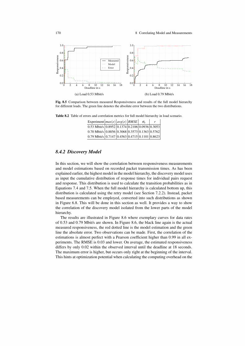
170 8 Correlating Model and Measurements
0.0
0.2
0.4
0.6
0.8
1.0
Res
pons
iven
ess
0 2 4 6 8 10 12 14 16 18Deadline in s
MeasuredModelError
(a) Load 0.53 Mbit/s
0.0
0.2
0.4
0.6
0.8
1.0
Res
pons
iven
ess
0 2 4 6 8 10 12 14 16 18Deadline in s
(b) Load 0.79 Mbit/s
Fig. 8.5 Comparison between measured Responsiveness and results of the full model hierarchyfor different loads. The green line denotes the absolute error between the two distributions.
Table 8.2 Table of errors and correlation metrics for full model hierarchy in load scenario.
Experiment max(e) avg(e) RMSE σe r0.53 Mbit/s 0.8952 0.1374 0.2106 0.0936 0.30530.70 Mbit/s 0.8856 0.3068 0.3573 0.1363 0.57620.79 Mbit/s 0.7147 0.4563 0.4715 0.1101 0.8623
8.4.2 Discovery Model
In this section, we will show the correlation between responsiveness measurementsand model estimations based on recorded packet transmission times. As has beenexplained earlier, the highest model in the model hierarchy, the discovery model usesas input the cumulative distribution of response times for individual pairs requestand response. This distribution is used to calculate the transition probabilities as inEquations 7.4 and 7.5. When the full model hierarchy is calculated bottom up, thisdistribution is calculated using the retry model (see Section 7.2.2). Instead, packetbased measurements can be employed, converted into such distributions as shownin Figure 6.8. This will be done in this section as well. It provides a way to showthe correlation of the discovery model isolated from the lower parts of the modelhierarchy.
The results are illustrated in Figure 8.6 where exemplary curves for data ratesof 0.53 and 0.79 Mbit/s are shown. In Figure 8.6, the black line again is the actualmeasured responsiveness, the red dotted line is the model estimation and the greenline the absolute error. Two observations can be made. First, the correlation of theestimations is almost perfect with a Pearson coefficient higher than 0.99 in all ex-periments. The RMSE is 0.03 and lower. On average, the estimated responsivenessdiffers by only 0.02 within the observed interval until the deadline at 18 seconds.The maximum error is higher, but occurs only right at the beginning of the interval.This hints at optimization potential when calculating the computing overhead on the

8.5 Experiments with Variable Radio Power 171
0.0
0.2
0.4
0.6
0.8
1.0
Res
pons
iven
ess
0 2 4 6 8 10 12 14 16 18Deadline in s
MeasuredModelError
(a) Load 0.53 Mbit/s
0.0
0.2
0.4
0.6
0.8
1.0
Res
pons
iven
ess
0 2 4 6 8 10 12 14 16 18Deadline in s
(b) Load 0.79 Mbit/s
Fig. 8.6 Comparison between measured Responsiveness and discovery model results for differentloads. The green line denotes the absolute error between the two distributions.
Table 8.3 Table of errors and correlation metrics for discovery model in load scenario.
Experiment max(e) avg(e) RMSE σe r0.53 Mbit/s 0.2079 0.0153 0.0300 0.0043 0.99490.70 Mbit/s 0.1144 0.0189 0.0288 0.0018 0.99750.79 Mbit/s 0.0544 0.0198 0.0248 0.0007 0.9988
node. However, the two distributions correlate very well and this validates the dis-covery model and especially its calculation of the transition probabilities for such ascenario. Table 8.3 sums up the values of the different error and correlation metrics.
8.5 Experiments with Variable Radio Power
In the second set of experiments, in each series a different radio signal power wasused on each of the mesh nodes. This changed the range of the wireless signal andin turn made it more vulnerable to interference and other types of faults. The resultsof the three series for antenna gains of 15, 18 and 20 dB are shown in Figure 8.7.
It can be seen when comparing Figure 8.7 and 8.4 that the overall responsivenessof both sets is similar. In fact, the antenna gain was chosen to resemble similar con-ditions for packet loss. However, contrary to the results from the load experimentsin Section 8.4 the slope of the CDF is a lot less smooth and the steps in the distri-bution due to the retries are considerably more pronounced. The reason for this isthat although the overall signal quality is lower and produces a comparable packetloss on the paths between requester and provider, the nodes do have to deal with lesstraffic as no background load is generated. Additionally, collisions happen only dueto the multicast flooding of SD packets or because of external interference. Bothcauses lead to a lower delay in the network, hence, sharper steps in the CDF.

172 8 Correlating Model and Measurements
0.6
0.8
1.0
Res
pons
iven
ess
0 2 4 6 8 10 12 14 16 18Deadline in s
20 dB18 dB15 dB
Fig. 8.7 Experimental CDF for power Experiments using antenna gains of 15, 18 and 20 dB.
8.5.1 Full Model Hierarchy
The results for the correlation of experiment and results of the full model hierarchyare shown in Figure 8.8. The experiment results reflect the black line correspondingto the line for the same load in Figure 8.4. The dotted red line are the estimationsof the model calculated bottom up. The dashed green line reflects the absolute error.Two exemplary graphs for antenna gains of 20 and 18 dB are shown.
As opposed to the results in Section 8.4.1, the two curves correlate considerablybetter. Especially with lower signal quality, the OLSR monitoring data seems to bet-ter pick up the actual transmission quality of the network and thus, the estimationof the full model hierarchy is consistently more accurate. With high signal qualitythe models overestimate responsiveness. What exactly causes this behavior cannotyet be fully explained. The behavior hints at the smaller OLSR probe packets beingless likely to be dropped than SD packets over higher quality links. More thoroughinvestigation is needed here. The RMSE is between 0.04 and 0.18 and the Pear-son coefficient is above 0.98 in two out of three series. The correlation in all threescenarios is promising, given that no additional measurements are needed to pro-duce such results but a current snapshot of the network is sufficient. All errors andcorrelation metrics are summarized in Table 8.4.
Table 8.4 Table of errors and correlation metrics for full model hierarchy in power scenario.
Experiment max(e) avg(e) RMSE σe r20 dB 0.7110 0.0696 0.1107 0.0443 0.881718 dB 0.2955 0.0216 0.0373 0.0071 0.982215 dB 0.2786 0.1767 0.1827 0.0148 0.9913

8.5 Experiments with Variable Radio Power 173
0.0
0.2
0.4
0.6
0.8
1.0
Res
pons
iven
ess
0 2 4 6 8 10 12 14 16 18Deadline in s
MeasuredModelError
(a) Gain 20 dB
0.0
0.2
0.4
0.6
0.8
1.0
Res
pons
iven
ess
0 2 4 6 8 10 12 14 16 18Deadline in s
(b) Gain 18 dB
Fig. 8.8 Comparison between measured responsiveness and results of the full model hierarchywith different antenna gain. The green line denotes the absolute error between the two distributions.
8.5.2 Discovery Model
Finally, we will show the correlation between responsiveness measurements withdifferent antenna gain and model estimations based on recorded packet transmissiontimes. Results are illustrated in Figure 8.9. The observations from Section 8.4.2 arevalid here as well. The correlation of the estimations is again almost perfect with r >0.99 in all experiments. The RMSE is 0.035 and lower. On average, the estimatedresponsiveness different by only 0.02 within the observed interval until the deadlineat 18 seconds. Also the maximum error is comparable to the load experiments sothe discovery model works equally well in both presented scenarios. This is strongevidence for the validity of the discovery model.
Another observation can be made in both the full model and discovery modelestimations. The retry steps in the CDF are steeper due to lower packet delays andthe maximum error shows spikes right after these retries. It shows that estimatingthe exact arrival times is non-trivial and the models struggle to capture it properly.However, even in those worst cases, the maximum error of the discovery model isstill between 0.24 and 0.09. In the latter case that means that predicting the respon-siveness at any given time will be at maximum 10% off and on average only 2%in all cases. Table 8.5 presents a summary of the obtained errors and correlationmetrics.
Table 8.5 Table of errors and correlation metrics for discovery model in power scenario.
Experiment max(e) avg(e) RMSE σe r20 dB 0.2426 0.0163 0.0353 0.0059 0.992218 dB 0.1687 0.0220 0.0334 0.0036 0.995715 dB 0.0905 0.0221 0.0295 0.0013 0.9964

174 8 Correlating Model and Measurements
0.0
0.2
0.4
0.6
0.8
1.0
Res
pons
iven
ess
0 2 4 6 8 10 12 14 16 18Deadline in s
(a) Gain 20 dB
0.0
0.2
0.4
0.6
0.8
1.0
Res
pons
iven
ess
0 2 4 6 8 10 12 14 16 18Deadline in s
MeasuredModelError
(b) Gain 18 dB
Fig. 8.9 Comparison between measured responsiveness and results of the discovery model withdifferent antenna gain. The green line denotes the absolute error between the two distributions.
8.5.3 One Hop Experiments
A separate set of experiments was run with only two neighboring nodes, to isolatethe SD operation from the rest of the network. The antenna gain was chosen to be at15 and 11 dB. In fact, it was rather difficult to choose correct values as the operatingsystem allows to set only integer values. This coarse grained resolution led to eitherperfect or non existent links if chosen too high or two low. At the same time, the gainneeded to be chosen such that one value provided consistently better quality then theother. Although both created a reasonably reliable link, 15 and 11 dB fulfilled theserequirements. Results are illustrated in Figure 8.10.
It can again be seen, that both the discovery model and the full model hierarchycorrelate well with the measured responsiveness. As before, the discovery modelfares consistently better as it relies on concrete SD packet measurements insteadof abstractions on the lower layers. For reference, Table 8.6 contains the numericalresults for this scenario.
Table 8.6 Table of errors and correlation metrics for one hop experiments in the power scenario.
Experiment model used max(e) avg(e) RMSE σe r
15 dBfull model 0.6679 0.0267 0.0621 0.0293 0.8229
discovery model 0.2589 0.0102 0.0349 0.0080 0.9888
11 dBfull model 0.6142 0.0348 0.0646 0.0242 0.8511
discovery model 0.2417 0.0105 0.0327 0.0068 0.9902

8.6 Conclusion 175
0.0
0.2
0.4
0.6
0.8
1.0
Res
pons
iven
ess
0 2 4 6 8 10 12 14 16 18Deadline in s
MeasuredModelError
(a) 15 db
0.0
0.2
0.4
0.6
0.8
1.0
Res
pons
iven
ess
0 2 4 6 8 10 12 14 16 18Deadline in s
MeasuredModelError
(b) 11 db
0.0
0.2
0.4
0.6
0.8
1.0
Res
pons
iven
ess
0 2 4 6 8 10 12 14 16 18Deadline in s
MeasuredModelError
(c) 15 db
0.0
0.2
0.4
0.6
0.8
1.0
Res
pons
iven
ess
0 2 4 6 8 10 12 14 16 18Deadline in s
MeasuredModelError
(d) 11 db
Fig. 8.10 Comparison between measured responsiveness and results of the full model hierarchyfor different values of signal strength.
8.6 Conclusion
We correlated model estimations for responsiveness with the actual measured re-sponsiveness during the same time interval. Two different estimations were calcu-lated. The first uses the full model hierarchy bottom up as presented in Section 7.5. Ituses input data about the links and their quality from the routing layer and uses it toapproximate the distribution of transmission times and probabilities over the pathsbetween the SD actors. This is done with the help of Probabilistic Breadth-FirstSearch (PBFS), which is described in Section 7.3. The second estimation is done bysolving only the discovery model using measurements of previous SD packets.
Both types of estimations may be feasible, depending on the application scenario.Using the full model hierarchy is advised if the network provides such low leveldata. Generally, this is true for wireless mesh networks with proactive routing. At thecost of computing resources for solving all models bottom up, network bandwidthis saved. Also, this estimation can be performed upon entering a network, no historyof measurements is needed. The second approach should be used if no low levelnetwork measurements are available. In this case, a history of SD operations should

176 8 Correlating Model and Measurements
be kept to be used as input data to the models. The more frequent SD operations areand the less dynamic the network is, this estimation will be more precise.
The estimations of the full model hierarchy depend highly on the quality of theinput data. Due to the experiment setup, the generated load did not have the sameimpact on the routing layer monitoring packets than it had on the SD packets. Thisuncertainty is inherited by the models which in these cases led to an overestimationof responsiveness. As soon as the low level monitoring data more closely reflects thequality of the SD communication, the model hierarchy estimations correlate betterwith the actual measurements. In these cases, the Root Mean Squared Error (RMSE)lies between 0.18 and 0.03 and the Pearson coefficient r is above 0.99 in two out ofthree cases while being 0.88 in the third. Still, more research is needed to improvethe quality of the input data. This in turn will automatically improve the quality ofthe models.
The correlation of the discovery model is exceptionally good. In fact, it correlatesnearly perfectly in all considered scenarios. The maximum error occurs only rightafter the requests and subsequent retries. This is due to the computing overheadon the client node being estimated outside the discovery model. A more preciseestimation will reduce this error. Still, the absolute error is between 0.05 and 0.24 inall scenarios. The RMSE is very low between 0.025 and 0.035 and r is well above0.99 in all scenarios. This validates the discovery model as a representation of theactive single SD process.
All error and correlation metrics are summarized in Table 8.7.
Table 8.7 Table of errors and correlation metrics in all scenarios.Scenario Experiment model used max(e) avg(e) RMSE σe r
Load
0.53 Mbit/sfull model 0.8952 0.1374 0.2106 0.0936 0.3053
discovery model 0.2079 0.0153 0.0300 0.0043 0.9949
0.70 Mbit/sfull model 0.8856 0.3068 0.3573 0.1363 0.5762
discovery model 0.1144 0.0189 0.0288 0.0018 0.9975
0.79 Mbit/sfull model 0.7147 0.4563 0.4715 0.1101 0.8623
discovery model 0.0544 0.0198 0.0248 0.0007 0.9988
Power
15 dBfull model 0.2786 0.1767 0.1827 0.0148 0.9913
discovery model 0.0905 0.0221 0.0295 0.0013 0.9964
18 dBfull model 0.2955 0.0216 0.0373 0.0071 0.9822
discovery model 0.1687 0.0220 0.0334 0.0036 0.9957
20 dBfull model 0.7110 0.0696 0.1107 0.0443 0.8817
discovery model 0.2426 0.0163 0.0353 0.0059 0.9922
Power 1-Hop11 dB
full model 0.6142 0.0348 0.0646 0.0242 0.8511discovery model 0.2417 0.0105 0.0327 0.0068 0.9902
15 dBfull model 0.6679 0.0267 0.0621 0.0293 0.8229
discovery model 0.2589 0.0102 0.0349 0.0080 0.9888

Part IVConclusions


Chapter 9Conclusions and Outlook
Abstract The results of the two main parts of this work are summarized and put intocontext. We first cover user-perceived service availability evaluation as presented inPart II. We then comment on the research on service discovery responsiveness inPart III and give pointers to future research.
9.1 User-Perceived Dependability
Services play an increasingly important role in modern networks, ranging from webservice provision of global businesses to the Internet of Things. Dependability ofservice provision is thus an important goal but the assessment of specific depend-ability properties remains challenging. Ever more often, a system-view of depend-ability does not properly reflect the variable distribution of dependability within dy-namic networks and is thus only of statistical relevance. Since providers and clientsare part of a connecting Information and Communications Technology (ICT) in-frastructure, service dependability varies with the position of actors. The ICT de-vices needed for service provision change for each configuration. Service depend-ability models need to incorporate these user-perceived perspectives. We presenttwo approaches to quantify user-perceived service dependability. Both approachesdemonstrate that the dependability of service provision indeed differs considerablydepending on the position of service clients and providers, even in highly reliablewired networks. The following sections hold concluding remarks for each problemarea that has been covered in the preceeding parts of this work.
We first focus on service availability. Using input models of the service, the in-frastructure and a mapping between the two to describe actors of service commu-nication, availability models are automatically created that calculate user-perceivedinstantaneous availability. The feasibility of the approach is demonstrated using ex-emplary services in the network of University of Lugano, Switzerland. The contri-butions of this approach as presented in Part II are being summarized in Section9.2.
179

180 9 Conclusions and Outlook
The second and main part of this thesis aims at the responsiveness of Service Dis-covery (SD), the probability to find service instances within a deadline even in thepresence of faults. For successful provision, a service first has to be discovered bya client so successful SD is a precondition for successful service usage. We presenta hierarchy of stochastic models to calculate user-perceived responsiveness of SDbased on monitoring data from the routing layer. Extensive series of experimentshave been run in the Distributed Embedded Systems (DES) wireless testbed at FreieUniversitat Berlin to assess responsiveness of current Service Discovery Protocols(SDPs) and to validate the presented models. The contributions of Part III can befound in in Section 9.3.
9.2 Service Availability Evaluation
A methodology is provided in Part II to facilitate the evaluation of user-perceivedservice dependability, that is, the dependability valid for a specific pairs service re-quester and provider. The approach is based on the work by Milanovic et al. [157]but we focus explicitly on instantaneous service availability and provide an auto-mated, fully model-driven methodology that evaluates user-perceived service avail-ability. In addition, the same methodology could be used to evaluate other depend-ability properties, given that different attributes necessary for evaluation of suchproperties are attributed to the ICT component model. All described features areachieved by transforming a set of input models that describe:
1. The ICT infrastructure, including non-functional properties related to the analy-sis of interest for every entity of the infrastructure.
2. An abstract service as a composition of atomic services, which are indivisiblewith respect to their functionality.
3. A mapping of atomic services to ICT components that enable these services,hence, the actors of service communication.
For the input models, the Unified Modeling Language (UML) was adopted forinfrastructure and service descriptions as it is standardized and widely used, espe-cially for design purposes. For the mapping model, the Extensible Markup Lan-guage (XML) was chosen due to its versatility. Visualization of the models has beenan important factor as well and these decisions guarantee that the models remainhuman-readable. The separation into individual models and distinct steps for gen-erating and using the models allows the methodology to be well suited for dynamicenvironments. Changes to intrinsic properties of network devices, such as failurerate, redundant components, manufacturer and others, can be performed directlyin the device class description and so reflect to all objects in the ICT infrastruc-ture model. That way, the methodology provides a straight-forward way to enabledifferent types of user-perceived dependability analysis based on a User-PerceivedService Infrastructure Model (UPSIM), depending on the properties for each classof components. The methodology uses a hierarchical service model with a compos-

9.2 Service Availability Evaluation 181
ite service on the highest level, which is composed of atomic services. The atomicservices in turn map to ICT infrastructure components. With only minor changesto this mapping model, all properties can be evaluated for different requesters andproviders, reflecting different user-perceived views.
Parts of the results of the research on service availability presented in this workhave been published in [2, 3, 5, 10, 12].
9.2.1 Output Models
The presented methodology provides an in major parts automated generation of dif-ferent output models for specified user-perceived views, such as a UPSIM for sub-sequent analysis, or Reliability Block Diagrams (RBDs) and Fault Trees (FTs) foravailability evaluation. The methodology uses specific instances of the previouslydescribed input models, which define the current state of the network, the serviceunder analysis and the user-perceived scope, and finds all ICT components relevantfor service provision of this pair, preserving their context within the network. It thengenerates a UPSIM that can be used in subsequent user-perceived dependabilityanalysis. We exemplify a transformation into a RBD, which is solved to obtain thesteady-state availability of the given service. Given deployment times of the ICTcomponents in the infrastructure model and usage durations in the service model,one main contribution of this methodology is a transformation into a RBD to assessinstantaneous service availability at a specific point in time. The approach definesa sound concept of service and component time to allow such analysis: In additionto the usage durations the exact component access times during provision are in-cluded in the service model and taken into account for evaluation, which results ina more accurate estimation, especially for longer service execution times. Insteadof an RBD, the methodology also supports and equivalent transformation to a FT.These output models for a client-specific infrastructure providing a composite ser-vice constitute a User-Perceived Service Availability Model (UPSAM).
9.2.2 Case Study
To demonstrate the proposed methodology, we apply it to parts of the service net-work infrastructure at University of Lugano (USI), Switzerland. We show how togenerate the UPSIM for an exemplary email service and demonstrate how such aUPSIM could be used to evaluate different user-perceived properties of the print-ing service for given service requesters and providers. As a side effect, with theUPSIM the methodology provides a practical way to automatically identify and vi-sualize dependability-relevant ICT components, to give a quick overview on wherethe service problem might be caused. Using the generated UPSAM, we show howthe steady-state availability of the same service can differ considerably even in such

182 9 Conclusions and Outlook
a high-availability network when requested from two different users. The methodol-ogy is thus able to provide a fine-grained view on service availability as experiencedfrom different points of the network. By using an UPSAM for instantaneous avail-ability evaluation, not only different views have been compared but also the impacton user-perceived service availability over time when modifying network compo-nents. As an example, the impact of redundant atomic service providers on the com-posite service availability was calculated. Additionally, individual ICT componentswere exchanged to demonstrate the effect of component age on availability. Theresults show availability as a dynamic property and indicate how the methodologycan improve network design by estimating the impact of new component deploy-ment. After deployment, they can be used to detect bottlenecks in the network or toevaluate the impact of planned changes to the ICT infrastructure.
9.2.3 Outlook
Although the demonstration network is based only on parts of the service networkat USI, the proposed methodology is scalable and applicable to complex, dynamicnetworks as well. We showed how different types of dynamics affect only specificmodels so that in most scenarios, the majority of models remains unchanged. Also,the methodology implementation is automated whenever no human input or deci-sion is necessary and it is thus possible to quickly regenerate the output models incase of dynamic changes to the network or its services. More research is needed todemonstrate the applicability of the methodology to complex infrastructures suchas cloud computing, which do not provide the operator with enough informationabout individual components necessary for service provision. Additionally, the pathdiscovery algorithm and creation of the composite reliability block diagram needoptimization when applied to networks with a high degree of connectivity, such aswireless mesh networks. Combining sets of components with a low variability inuser-perceived availability to reduce the size of the topology graph should be con-sidered. Finally, extending the methodology to evaluate different time-dependentdependability properties like performability remains an open issue. With respect toinstantaneous availability, future work should focus on improving the accuracy ofthe resulting availability estimation especially with respect to short term effects onthe infrastructure. This includes examining extensions to support variable failureand repair rates and a proper load model.
9.3 Evaluation of Service Discovery Responsiveness
Part III provides an extensive evaluation of the responsiveness of SD, the proba-bility to successfully discover service providers within deadlines. To the best ofour knowledge, no work has been done that covers an evaluation of this impor-

9.3 Evaluation of Service Discovery Responsiveness 183
tant property both by experiments and using stochastic models. Results of the re-search on SD responsiveness presented in this work have in parts been published in[3, 1, 4, 6, 7, 9, 11, 8].
9.3.1 Experimental Evaluation
First, we examined the dependability of decentralized active SD in experiments, toobserve the behavior of SD responsiveness in three common scenarios. This hasbeen done in two experiment environments. First, a hypervisor based virtual testbedand second, the Distributed Embedded Systems (DES) wireless testbed at Freie Uni-versitat Berlin (FUB). In the DES testbed, the ExCovery experiment framework wasemployed to run all series of experiments. Responsiveness of Domain Name System(DNS) based discovery was evaluated under varying fault intensity and with up to50 service instances. Furthermore, we analyzed the impact of the deadline of the SDoperation, the distance of nodes, the load in the network and the required numberof providers to be discovered. Analysis in the DES testbed was performed both forthe individual discovery packets as well as the complete discovery operation, whichincludes retries in case packets do not arrive in time. The former allows to inferconclusions for other application protocols which use similar packets and can pro-vide input for existing and future analytical models which use lower network levelmeasurements. The analysis provides an extensive evaluation of SD responsivenesswith a realistic fault model. Presented results are applicable to various types of op-timizations in wireless mesh networks.
The results in the virtual testbed show that the responsiveness of the used SDPsdecreases dramatically with moderate packet loss of around 20%. It decreases non-proportional when more service instances need to be discovered. At higher packetloss rates the decrease becomes exponential with the number of nodes to be discov-ered such that SD becomes practically impossible. Responsiveness can be improvedif a low coverage is acceptable. This can be the case, for example, if redundantservice instances are introduced to the network and only a fixed number of serviceinstances needs to be discovered, regardless of the total number of instances in thenetwork. However, this assumption is only valid in networks with low packet loss.In less reliable networks, redundant service instances and the caused overhead incommunication could in fact worsen responsiveness.
In addition to the experiments on SD, an analysis of the long-term behavior ofthe DES testbed and the effects of internal and external faults was carried out. In-ternal faults contain node crashes or clock drifts, external faults comprise all typesof wireless interference or also forced interruptions during experiment execution. Ithas been shown that the effect of these faults is considerable and has to be taken intoaccount when interpreting results. Experiment analysis based on average measure-ments should be done very carefully. Choosing the measurement history windowsize too big can easily lead to over or underestimating of the testbed link quality.

184 9 Conclusions and Outlook
Experiment Environment ExCovery
The experiment framework ExCovery developed for this work has been tried and re-fined in a manifold of SD dependability experiments over the last two years, whichwere carried out on the wireless DES testbed at FUB. The core of ExCovery is aformal experiment description that supports automated checking, execution and ad-ditional features, such as visualization of experiments. In addition to that, the frame-work offers unified concepts for experiment execution, measurement and storage ofresults. As such, ExCovery is expected to foster experiment repeatability, compa-rability and transparency. To support this claim and to facilitate transparency andrepeatability, all experiment descriptions and results of this work are made availablefor interested researchers on request. ExCovery is available for download in a publicrepository under the permissive MIT license [8].
ExCovery was specifically developed for the experiments on SD presented inChapters 6 and 8 but has generic support for experiments on the dependability ofdistributed processes. We provided an abstract description of SD as experiment pro-cess. The description covers the specification of the individual processes of an ex-periment and their actors: Fault injection, environment manipulation and the mainprocess under experimentation (in this case SD) are expressed as interdependent se-ries of actions and events. Execution takes care of controlling the individual nodesduring experiment runtime, to make sure each run of an experiment has a clean anddefined environment and each node acts according to the experiment description.ExCovery manages series of experiments and recovers from failures by resumingaborted runs. Measurements are taken both on the level of experiment process ac-tions and events, to record the behavior as seen by the application, and on the levelof raw network packets. Measurements are stored in a unified database format tofacilitate sharing and comparison of results. ExCovery has already been employedin a number of works from other authors and is still under active development.
9.3.2 Stochastic Modeling
This work proposes a stochastic model family to evaluate the user-perceived respon-siveness of active decentralized SD. The family consists of a hierarchy of Markovand semi-Markov processes that are parametrized to allow instantiation for diverseSD scenarios and use current network monitoring data as input. To put the modelsinto use, a methodology is introduced that works specifically in wireless mesh net-works with proactive routing. Upon request, the methodology generates and solvesmodel instances bottom up for specific SD scenarios. Especially the abstractionsat the lower layers lead to a comparably low complexity, which allows for diverseaggregate calculations, such as the average responsiveness of one provider for allclients in the network. The methodology relies on the Monte Carlo method Proba-bilistic Breadth-First Search (PBFS) to estimate the behavior of SD multicast com-munication. PBFS was developed during the work on this dissertation and approx-

9.3 Evaluation of Service Discovery Responsiveness 185
imates the reachability and other metrics of network-wide broadcasts by randomsampling the packet traversal through a probabilistic graph.
Using monitoring data from the DES testbed, responsiveness is evaluated for thethree most prevalent SDPs in IP networks: Service Location Protocol (SLP), SimpleService Discovery Protocol (SSDP) and Zeroconf discovery. First, the responsive-ness for different pairs of requester and provider is compared. Second, the averageresponsiveness of a single provider, depending on the topology, is analyzed. Resultsdemonstrate that responsiveness varies dramatically depending on the position ofnodes in the network and the overall link quality. Thus, they confirm the findingsfrom the experiments. The results further indicate that, with short deadlines close tothe individual retry intervals, the right retry timing strategy is more important thanthe communication mechanism. With longer deadlines, using the more reliable uni-cast instead of multicast consistently improves responsiveness. In either case, thefixed strategies of current SDPs struggle to achieve a high responsiveness in thesedynamic and inherently unreliable networks. Finally, a new metric expected respon-siveness distance der is introduced, estimating the maximum hop distance from aprovider at which nodes can discover it with a required responsiveness. To deploy aresponsive service with a minimum number of nodes, every requester in the networkshould be within the der of at least one provider. The der of two different providers isevaluated and the results underline the importance of position when placing serviceinstances.
Validation shows that the highest layer discrete time Markov model, which rep-resents the SDP itself, is able to estimate the actual measured responsiveness with avery low error at any given time. It uses input data in the form of a distribution ofresponse times of previous discovery operations. Model estimations and experimentmeasurements consistently converge to the same value and correlate with a rootmean squared error of 0.03 and below in all cases. The Pearson product-momentcorrelation coefficient r is well above 0.99 in all cases. This validates the model asa proper representation of the discovery operation. The lower layer models, whichcalculate the probability and time distribution of traversal for specific network pack-ets, are able to estimate the actual behavior with a low error under the condition thatthe input data properly reflects the current network quality. It has been shown thatthe used Expected Transmission Count (ETX) metric, as given by the routing layer,has its shortcomings and cannot always cope with the dynamics of wireless linkqualities. The quality of the ETX metric increases the more static the network is,thus reducing the error of the estimations given by the presented stochastic models.We can conclude that given a precise metric of the link quality, the complete hier-archy of stochastic models is able to estimate the responsiveness for any given SDcommunication pair with a high accuracy.

186 9 Conclusions and Outlook
9.3.3 Outlook
Responsiveness evaluation of SD in dynamic and decentralized networks remainschallenging. With increasing demand for real-time systems, responsiveness opti-mization will become one of the main issues. With self-configuring networks enter-ing dependability critical domains, our experimental and analytical evaluation hasshown that distributed SD has to be used with caution, especially in wireless sce-narios where packet loss cannot be neglected. Applying advanced cache optimiza-tions to reduce transmissions as proposed in [45] could improve responsiveness insuch scenarios. Optimizing retry strategies seems to be indeed one promising nextstep. However, further investigations are needed since not all improvements wouldbe compliant with existing standards that are already deployed in current networkdevices. Some adaptations such as accepting non-authoritative discovery responsesfrom any node in the service network might improve discovery responsiveness butreduce the reliability of service discovery as a whole.
Future research could extend the presented hierarchy of stochastic models to sup-port centralized and hybrid SD architectures. Also, the higher layer discovery modelis not time-dependent and needs to be regenerated for different deadlines if the num-ber of retries changes. The probability Pe to transition to the error state after the lastretry needs to be calculated for each deadline. However, the discovery model pro-vides an intuitive representation of the SDP communication and can be calculatedwith low complexity. These advantages are important when optimizing SDPs forfixed deadlines as given by the application layer. Nevertheless, the time dependenceof the lower layer models could be combined in a single discovery layer modelwhich uses the deadline as a parameter and calculates the distribution of arrivaltimes in the absorbing states. This in turn could be used to assess responsiveness.Such model could then support the development of novel SDPs that, for example,support variable retry intervals depending on the state of the network.

9.3 Evaluation of Service Discovery Responsiveness 187
Final Remarks
The main contributions of this dissertation are two different methodologies for user-perceived dependability evaluation in service networks. Both methodologies havethe same foundation, to generate models for dependability evaluation bottom upbased on the current monitored state of the network and to allow a time-dependentdependability evaluation using these models. This way, they enable optimization ofservice networks with respect to known or predicted usage patterns.
The presented solutions can be used in service networks to analyze the qual-ity of service deployments for different client perspectives. Service discovery is anintegral parts of such deployments. Furthermore, they help to improve them by es-timating the quality when placing additional instances, moving existing instancesand adding or replacing network equipment. Since the user-perspective is valid forboth the clients and providers, both parties may use the models given that they havesufficient input data to generate and solve them.
Finally, the methodologies developed in this work are one step away from antic-ipating novel service dependability models which combine service discovery, time-liness, placement and usage, areas that until now have been treated to a large extentseparately. Such models will become the basis for future adaptive and autonomousnetworks such as the Internet of Things and its successors.


References to Works of the Author
1. Dittrich, A.: Self-aware adaptive service networks with dependability guarantees. In: K. Bol-lue, D. Guckel, U. Loup, J. Sponemann, M. Winkler (eds.) Joint Workshop of the GermanResearch Training Groups in Computer Science, p. 88. Verlagshaus Mainz, Aachen, Germany(2010). Extended abstract
2. Dittrich, A., Kaitovic, I., Murillo, C., Rezende, R.: A model for evaluation of user-perceivedservice properties. In: 27th International Parallel & Distributed Processing Symposium, Work-shops and Phd Forum (IPDPSW), pp. 1508–1517. IEEE Computer Society, Boston, MA, USA(2013). doi:10.1109/IPDPSW.2013.163
3. Dittrich, A., Kowal, J., Malek, M.: Designing survivable services from independent compo-nents with basic functionality. In: International Workshop on Dependable Network Comput-ing and Mobile Systems (DNCMS), pp. 33–38. IEEE Computer Society, Naples, Italy (2008).doi:10.13140/2.1.1438.3684
4. Dittrich, A., Lichtblau, B., Rezende, R., Malek, M.: Modeling responsiveness of decentralizedservice discovery in wireless mesh networks. In: K. Fischbach, U.R. Krieger (eds.) MMB &DFT, Lecture Notes in Computer Science, vol. 8376, chap. 7, pp. 88–102. Springer Interna-tional Publishing (2014). doi:10.1007/978-3-319-05359-2 7
5. Dittrich, A., Rezende, R.: Model-driven evaluation of user-perceived service availability. In:M. Vieira, J.C. Cunha (eds.) Dependable Computing, Lecture Notes in Computer Science, vol.7869, pp. 39–53. Springer Berlin Heidelberg (2013). doi:10.1007/978-3-642-38789-0 4
6. Dittrich, A., Salfner, F.: Experimental responsiveness evaluation of decentralized service dis-covery. In: 24th International Parallel & Distributed Processing Symposium, Workshopsand Phd Forum (IPDPSW), pp. 1–7. IEEE Computer Society, Atlanta, GA, USA (2010).doi:10.1109/IPDPSW.2010.5470861
7. Dittrich, A., Solis Herrera, D., Coto, P., Malek, M.: Responsiveness of service discovery inwireless mesh networks. In: 20th Pacific Rim International Symposium on Dependable Com-puting (PRDC). IEEE Computer Society, Singapore (2014). doi:10.1109/PRDC.2014.38
8. Dittrich, A., Wanja, S.: ExCovery – a framework for distributed system experiments. Softwarerepository (2014). Version 0.2, Published under the MIT License. URL http://adittrich.github.io/excovery
9. Dittrich, A., Wanja, S., Malek, M.: ExCovery – a framework for distributed system exper-iments and a case study of service discovery. In: 28th International Parallel & DistributedProcessing Symposium, Workshops and Phd Forum (IPDPSW), pp. 1314–1323. IEEE Com-puter Society, Phoenix, AZ, USA (2014). doi:10.1109/IPDPSW.2014.147
10. Goldschmidt, T., Dittrich, A., Malek, M.: Quantifying criticality of dependability-related itorganization processes in cobit. In: 15th Pacific Rim International Symposium on Depend-able Computing (PRDC), pp. 336–341. IEEE Computer Society, Shanghai, China (2009).doi:10.1109/PRDC.2009.60
189

190 References to Works of the Author
11. Lichtblau, B., Dittrich, A.: Probabilistic breadth-first search – a method for evaluation ofnetwork-wide broadcast protocols. In: 6th IEEE/ACM/IFIP International Conference on NewTechnologies, Mobility and Security (NTMS). IEEE Computer Society, Dubai, UAE (2014).doi:10.1109/NTMS.2014.6814046
12. Rezende, R., Dittrich, A., Malek, M.: User-perceived instantaneous service availability evalu-ation. In: 19th Pacific Rim International Symposium on Dependable Computing (PRDC), pp.273–282. IEEE Computer Society, Vancouver, Canada (2013). doi:10.1109/PRDC.2013.49

References
13. The NS-3 network simulator. Webpage (2012). URL http://www.nsnam.org14. Aboba, B., Thaler, D., Esibov, L.: Link-local multicast name resolution (LLMNR). RFC
4795 (Informational) (2007)15. Akyildiz, I.F., Su, W., Sankarasubramaniam, Y., Cayirci, E.: Wireless sensor networks: a
survey. Computer Networks 38(4), 393–422 (2002). doi:10.1016/S1389-1286(01)00302-416. Akyildiz, I.F., Wang, X., Wang, W.: Wireless mesh networks: a survey. Computer Networks
47(4), 445–487 (2005). doi:10.1016/j.comnet.2004.12.00117. Apache Software Foundation: Apache River - JiniTM Network Technology Specifications,
2.2.2 edn. (2013)18. Arabshian, K., Schulzrinne, H.: Gloserv: global service discovery architecture. In: 1st An-
nual International Conference on Mobile and Ubiquitous Systems: Networking and Services(MOBIQUITOUS), pp. 319–325 (2004). doi:10.1109/MOBIQ.2004.1331738
19. Armbrust, M., Fox, A., Griffith, R., Joseph, A.D., Katz, R.H., Konwinski, A., Lee, G., Patter-son, D.A., Rabkin, A.I.S.M.Z.: Above the clouds: A berkeley view of cloud computing. Tech.Rep. UCB/EECS-2009-28, UC Berkeley Reliable Adaptive Distributed Systems Laboratory(2009)
20. ARTEMIS Embedded Computing Systems Initiative: CHESS project. Webpage (2012).URL http://www.chess-project.org
21. Atzori, L., Iera, A., Morabito, G.: The internet of things: A survey. Computer Networks54(15), 2787–2805 (2010). doi:10.1016/j.comnet.2010.05.010
22. The avahi project. Software (2014). URL http://avahi.org23. Avizienis, A., Laprie, J.C., Randell, B., Landwehr, C.: Basic concepts and taxonomy of de-
pendable and secure computing. IEEE Transactions on Dependable and Secure Computing1(1), 11–33 (2004). doi:10.1109/TDSC.2004.2
24. Bailey, R.A.: Design of Comparative Experiments, Cambridge Series in Statistical and Prob-abilistic Mathematics, vol. 25. Cambridge University Press (2008)
25. Barborak, M., Dahbura, A., Malek, M.: The consensus problem in fault-tolerant computing.ACM Computing Surveys 25(2), 171–220 (1993). doi:10.1145/152610.152612
26. Baresi, L., Guinea, S.: Towards dynamic monitoring of WS-BPEL processes. In: Service-Oriented Computing - (ICSOC) 2005, Lecture Notes in Computer Science, vol. 3826, pp.269–282. Springer Berlin Heidelberg (2005). doi:10.1007/11596141 21
27. Barham, P.R., Dragovic, B., Fraser, K.A., Hand, S.M., Harris, T.L., Ho, A.C., Kotsovinos,E., Madhavapeddy, A.V.S., Neugebauer, R., Pratt, I.A., Warfield, A.K.: Xen 2002. Tech.Rep. UCAM-CL-TR-553, University of Cambridge, 15 JJ Thomson Avenue, Cambridge,UK (2003)
28. Beaudry, M.: Performance-related reliability measures for computing systems. IEEE Trans-actions on Computers 27(6), 540–547 (1978). doi:10.1109/TC.1978.1675145
191

192 References
29. Ben Mokhtar, S., Preuveneers, D., Georgantas, N., Issarny, V., Berbers, Y.: Easy: Efficient se-mAntic Service discoverY in pervasive computing environments with QoS and context sup-port. Journal of Systems and Software 81(5), 785–808 (2008). doi:10.1016/j.jss.2007.07.030.Software Process and Product Measurement
30. Bernardi, S., Merseguer, J., Petriu, D.: An UML profile for dependability analysis and mod-eling of software systems. Tech. Rep. RR-08-05, University of Zaragoza (2008)
31. Bettstetter, C., Renner, C.: A comparison of service discovery protocols and implementationof the service location protocol. In: 6th EUNICE Open European Summer School: InnovativeInternet Applications (2000)
32. Bezivin, J., Gerbe, O.: Towards a precise definition of the OMG/MDA framework. In: 16th
Annual International Conference on Automated Software Engineering (ASE), pp. 273–280.IEEE Computer Society Press (2001). doi:10.1109/ASE.2001.989813
33. Bianchi, G.: Performance analysis of the IEEE 802.11 distributed coordination func-tion. IEEE Journal on Selected Areas in Communications 18(3), 535–547 (2000).doi:10.1109/49.840210
34. Bittanti, S., Campi, M.C., Prandini, M.: How many experiments are needed to adapt? In:A. Chiuso, S. Pinzoni, A. Ferrante (eds.) Modeling, Estimation and Control, Lecture Notesin Control and Information Sciences, vol. 364, pp. 5–14. Springer Berlin Heidelberg (2007).doi:10.1007/978-3-540-73570-0 2
35. Bluetooth SIG, Inc.: Specification of the Bluetooth System, 4.1 edn. (2013)36. Blywis, B., Gunes, M., Juraschek, F., Hahm, O.: Properties and topology of the DES-testbed.
Tech. Rep. TR-B-11-02, Freie Universitat Berlin, Computer Systems & Telematics, Takus-traße 9, 14195 Berlin, Germany (2011)
37. Blywis, B., Reinecke, P., Gunes, M., Wolter, K.: Gossip routing, percolation, andrestart in wireless multi-hop networks. In: Wireless Communications and Net-working Conference (WCNC), pp. 3019–3023. IEEE Computer Society (2012).doi:10.1109/WCNC.2012.6214322
38. Bocciarelli, P., D’Ambrogio, A.: Model-driven performability analysis of composite webservices. In: SIPEW, pp. 228–246 (2008). doi:10.1007/978-3-540-69814-2 15
39. Bohnenkamp, H., van der Stok, P., Hermanns, H., Vaandrager, F.: Cost-optimizationof the IPv4 zeroconf protocol. In: International Conference on Dependable Systemsand Networks, pp. 531–540. IEEE Computer Society, Los Alamitos, CA, USA (2003).doi:10.1109/DSN.2003.1209963
40. Bondavalli, A., Lollini, P., Montecchi, L.: Analysis of user perceived qos in ubiquitousumts environments subject to faults. In: U. Brinkschulte, T. Givargis, S. Russo (eds.)Software Technologies for Embedded and Ubiquitous Systems (SEUS), Lecture Notes inComputer Science, vol. 5287, chap. 17, pp. 186–197. Springer Berlin Heidelberg (2008).doi:10.1007/978-3-540-87785-1 17
41. Bosse, S., Schulz, C., Turowski, K.: Predicting availability and response times of IT services.In: 22nd European Conference on Information Systems (ECIS). Tel Aviv, Israel (2014)
42. Brandes, U., Erlebach, T. (eds.): Network Analysis – Methodological Foundations,Lecture Notes in Computer Science, vol. 3418. Springer Berlin Heidelberg (2005).doi:10.1007/b106453
43. Bruning, S., Weissleder, S., Malek, M.: A fault taxonomy for service-oriented architecture.In: Informatik-Berichte, vol. 215. Humboldt-Universitat zu Berlin, Institut fur Informatik(2007)
44. Bruning, S., Weissleder, S., Malek, M.: A fault taxonomy for service-oriented architecture.In: 10th High Assurance Systems Engineering Symposium (HASE), pp. 367–368. IEEEComputer Society (2007). doi:10.1109/HASE.2007.46
45. Campo, C., Garcıa-Rubio, C.: DNS-based service discovery in ad hoc networks: Evaluationand improvements. In: P. Cuenca, L. Orozco-Barbosa (eds.) Personal Wireless Communica-tions, Lecture Notes in Computer Science, vol. 4217, pp. 111–122. Springer Berlin Heidel-berg (2006). doi:10.1007/11872153 10

References 193
46. Cardoso, J., Sheth, A., Miller, J., Arnold, J., Kochut, K.: Quality of service for workflowsand web service processes. Web Semantics: Science, Services and Agents on the WorldWide Web 1(3), 281–308 (2004). doi:10.1016/j.websem.2004.03.001
47. Cervantes, H., Hall, R.: Autonomous adaptation to dynamic availability using a service-oriented component model. In: 26th International Conference on Software Engineering(ICSE), pp. 614–623. IEEE Computer Society (2004). doi:10.1109/ICSE.2004.1317483
48. Chakraborty, D., Joshi, A., Yesha, Y., Finin, T.: Toward distributed service discovery in per-vasive computing environments. Transactions on Mobile Computing 5(2), 97–112 (2006).doi:10.1109/TMC.2006.26
49. Chan, K.S.M., Bishop, J., Steyn, J., Baresi, L., Guinea, S.: A fault taxonomy for web servicecomposition. In: 3rd International Workshop on Engineering Service Oriented Applications(WESOA), Lecture Notes in Computer Science, vol. 4907, pp. 363–375. Springer (2007).doi:10.1007/978-3-540-93851-4 36
50. Chen, P., Johansson, K.H., Balister, P., Bollobas, B., Sastry, S.: Multi-path routing metricsfor reliable wireless mesh routing topologies. Tech. Rep. TRITA-EE 2011:033, KTH RoyalInstitute of Technology, SE-100 44 Stockholm, Sweden (2011)
51. Cheshire, S.: Zero configuration networking (zeroconf). Webpage (2009). URL http://www.zeroconf.org
52. Cheshire, S., Aboba, B., Guttman, E.: Dynamic configuration of IPv4 link-local addresses.RFC 3927 (Proposed Standard) (2005)
53. Cheshire, S., Krochmal, M.: DNS-based service discovery. RFC 6763 (Proposed Standard)(2013)
54. Cheshire, S., Krochmal, M.: Multicast DNS. RFC 6762 (Proposed Standard) (2013)55. Cheshire, S., Steinberg, D.H.: Zero Configuration Networking - The Definitive Guide, 1st
edn. O’Reilly Media (2005)56. Ciardo, G., Marie, R.A., Sericola, B., Trivedi, K.S.: Performability analysis using semi-
markov reward processes. IEEE Transactions on Computers 39(10), 1251–1264 (1990).doi:10.1109/12.59855
57. Clausen, T., Jacquet, P.: Optimized link state routing protocol (OLSR). RFC 3626 (Experi-mental) (2003)
58. Controneo, D., di Flora, C., Russo, S.: Improving dependability of service oriented architec-tures for pervasive computing. In: 8th International Workshop on Object-Oriented Real-TimeDependable Systems (WORDS), pp. 74–81 (2003). doi:10.1109/WORDS.2003.1218068
59. Cordeiro, W., Aguiar, E., Moreira, W., Abelem, A., Stanton, M.: Providing quality ofservice for mesh networks using link delay measurements. In: 16th International Con-ference on Computer Communications and Networks (ICCCN), pp. 991–996 (2007).doi:10.1109/ICCCN.2007.4317947
60. Cormen, T.H., Stein, C., Rivest, R.L., Leiserson, C.E.: Introduction to Algorithms, 2 edn.McGraw-Hill Higher Education (2001)
61. Coto, P.: Responsiveness analysis of service location protocol in wireless mesh testbed. Mas-ter’s thesis, Universita della Svizzera Italiana (USI), Lugano, Switzerland (2014)
62. Couto, D.S.J.D., Aguayo, D., Bicket, J., Morris, R.: A high-throughput path metric for multi-hop wireless routing. In: 9th annual international conference on Mobile computing and net-working, pp. 134–146. ACM, San Diego, USA (2003). doi:10.1145/938985.939000
63. Cristian, F.: Understanding fault-tolerant distributed systems. ACM Communications 34(2),56–78 (1991). doi:10.1145/102792.102801
64. Czarnecki, K., Helsen, S.: Feature-based survey of model transformation approaches. IBMSystems Journal 45(3), 621–645 (2006). doi:10.1147/sj.453.0621
65. Czerwinski, S.E., Zhao, B.Y., Hodes, T.D., Joseph, A.D., Katz, R.H.: An architecture for asecure service discovery service. In: 5th Annual ACM/IEEE International Conference onMobile Computing and Networking (MobiCom)International Conference on Mobile Com-puting and Networking (MobiCom), MobiCom ’99, pp. 24–35. ACM, Seattle, Washington,USA (1999). doi:10.1145/313451.313462

194 References
66. Dabrowski, C.E., Mills, K.L.: Analyzing properties and behavior of service discovery pro-tocols using an architecture-based approach. In: Working Conference on Complex and Dy-namic Systems Architecture (2001)
67. Dabrowski, C.E., Mills, K.L.: Understanding self-healing in service-discovery sys-tems. In: Workshop on Self-healing systems (WOSS), pp. 15–20. ACM (2002).doi:10.1145/582128.582132
68. Dabrowski, C.E., Mills, K.L., Elder, J.: Understanding consistency maintenance in ser-vice discovery architectures during communication failure. In: 3rd International Work-shop on Software and Performance (WOSP), pp. 168–178. ACM, Rome, Italy (2002).doi:10.1145/584369.584396
69. Dabrowski, C.E., Mills, K.L., Elder, J.: Understanding consistency maintenance in servicediscovery architectures in response to message loss. In: 4th Annual International Workshopon Active Middleware Services, pp. 51–60 (2002). doi:10.1109/AMS.2002.1029690
70. Dabrowski, C.E., Mills, K.L., Quirolgico, S.: A model-based analysis of first-generation ser-vice discovery systems. Tech. Rep. ADA523379, NIST National Institute of Standards andTechnology, Gaithersburg, MD, USA (2005)
71. Dabrowski, C.E., Mills, K.L., Quirolgico, S.: Understanding failure response in service dis-covery systems. J. Syst. Softw. 80(6), 896–917 (2007). doi:10.1016/j.jss.2006.11.017
72. Dabrowski, C.E., Mills, K.L., Rukhin, A.: Performance of service-discovery architectures inresponse to node failures. Tech. Rep. ADA511255, NIST National Institute of Standards andTechnology, Gaithersburg, MD, USA (2003)
73. Dai, Y.S., Xie, M., Poh, K.L., Liu, G.Q.: A study of service reliability and availability for dis-tributed systems. Reliability Engineering & System Safety 79(1), 103–112 (2003). doi:DOI:10.1016/S0951-8320(02)00200-4
74. Dean, A., Voss, D. (eds.): Design and Analysis of Experiments. Springer Texts in Statistics.Springer New York (1999). doi:10.1007/b97673
75. Debian – the universal operating system. Webpage (2013). URL http://www.debian.org76. Derrick, T.R., Bates, B.T., Dufek, J.S.: Evaluation of time-series data sets using the pearson
product-moment correlation coefficient. Medicine and science in sports and exercise 26(7),919—928 (1994)
77. Ding, Z., Chen, Z., Liu, J.: A rigorous model of service component architecture. ElectronicNotes in Theoretical Computer Science 207, 33–48 (2008). doi:10.1016/j.entcs.2008.03.084
78. Duda, A.: Understanding the performance of 802.11 networks. In: 19th International Sym-posium on Personal, Indoor and Mobile Radio Communications (PIMRC), pp. 1–6. IEEEComputer Society (2008). doi:10.1109/PIMRC.2008.4699942
79. Edwards, W.K.: Discovery systems in ubiquitous computing. IEEE Pervasive Computing5(2), 70–77 (2006). doi:10.1109/MPRV.2006.28
80. Enneya, N., Oudidi, K., Elkoutbi, M.: Enhancing delay in manet using olsr protocol. Inter-national Journal of Communications, Network and System Sciences 2(5), 392–399 (2009).doi:10.4236/ijcns.2009.25044
81. Erl, T.: Service-Oriented Architecture: Concepts, Technology, and Design, 1st edn. The Pren-tice Hall Service Technology Series from Thomas Erl. Prentice Hall PTR, Upper SaddleRiver, NJ, USA (2005)
82. Esposito, P.M., Campista, M.E.M., Moraes, I.M., Costa, L.H.M.K., Duarte, O.C.M.B., Ru-binstein, M.G.: Implementing the expected transmission time metric for olsr wireless meshnetworks. In: 1st IFIP Wireless Days (WD), pp. 1–5 (2008). doi:10.1109/WD.2008.4812900
83. Eusgeld, I., Fechner, B., Salfner, F., Walter, M., Limbourg, P., Zhang, L.: Hardware Relia-bility, chap. 9, pp. 59–103. Vol. 4909 of Eusgeld et al. [85] (2008). doi:10.1007/978-3-540-68947-8 9
84. Eusgeld, I., Fraikin, F., Rohr, M., Salfner, F., Wappler, U.: Software Reliability, chap. 10, pp.104–125. Vol. 4909 of Eusgeld et al. [85] (2008). doi:10.1007/978-3-540-68947-8 10
85. Eusgeld, I., Freiling, F.C., Reussner, R. (eds.): Dependability Metrics, Advanced Lec-tures, Lecture Notes in Computer Science, vol. 4909. Springer Berlin Heidelberg (2008).doi:10.1007/978-3-540-68947-8

References 195
86. Eusgeld, I., Happe, J., Limbourg, P., Rohr, M., Salfner, F.: Performability, chap. 24, pp. 245–254. Vol. 4909 of Eusgeld et al. [85] (2008). doi:10.1007/978-3-540-68947-8 24
87. Even, S.: Graph Algorithms, 2nd edn. Cambridge University Press (2011)88. Feitelson, D.G.: Experimental computer science: The need for a cultural change. Tech. rep.,
The Hebrew University of Jerusalem (2006). Manuscript89. Flores-Cortes, C.A., Blair, G.S., Grace, P.: An adaptive middleware to overcome service
discovery heterogeneity in mobile ad hoc environments. IEEE Distributed Systems Online8(7) (2007). doi:10.1109/MDSO.2007.41
90. Fussell, D.S., Malek, M. (eds.): Responsive Computer Systems: Steps Toward Fault-TolerantReal-Time Systems. Kluwer Academic Publishers (1995). doi:10.1007/978-1-4615-2271-3
91. Gershenfeld, N., Krikorian, R., Cohen, D.: The internet of things. Scientific American291(4), 76–81 (2004)
92. Giordano, M.: Dns-based discovery system in service oriented programming. In: P.M.A.Sloot, A.G. Hoekstra, T. Priol, A. Reinefeld, M. Bubak (eds.) Advances in Grid Computing(EGC), Lecture Notes in Computer Science, vol. 3470, pp. 840–850. Springer Berlin Heidel-berg (2005). doi:10.1007/11508380 86
93. Goland, Y.Y., Cai, T., Leach, P., Gu, Y.: Simple service discovery protocol/1.0 – operatingwithout an arbiter. Internet Draft (1999). URL ftp://ftp.pwg.org/pub/pwg/ipp/new SSDP/draft-cai-ssdp-v1-03.txt
94. Goldschmidt, T., Malek, M.: Ranking of dependability-relevant indicators for availabilityenhancement of enterprise information systems. Tech. rep., Humboldt-Universitat zu Berlin(2012)
95. Gorbenko, A., Kharchenko, V., Tarasyuk, O., Chen, Y., Romanovsky, A.: The threat of un-certainty in service-oriented architecture. In: RISE/EFTS Joint International Workshop onSoftware Engineering for Resilient Systems (SERENE), pp. 49–54. ACM, New York, NY,USA (2008). doi:10.1145/1479772.1479781
96. Grassi, V., Mirandola, R., Sabetta, A.: A model-driven approach to performability analysisof dynamically reconfigurable component-based systems. In: 6th International Workshopon Software and Performance (WOSP), pp. 103–114. ACM, New York, NY, USA (2007).doi:10.1145/1216993.1217011
97. Gray, J.: Why do computers stop and what can be done about it? Tech. Rep. TR-85.7, Tandem(1985)
98. Grottke, M., Sun, H., Fricks, R.M., Trivedi, K.S.: Ten fallacies of availability and reliabilityanalysis. In: T. Nanya, F. Maruyama, A. Pataricza, M. Malek (eds.) Service Availability,Lecture Notes in Computer Science, vol. 5017, pp. 187–206. Springer Berlin Heidelberg(2008). doi:10.1007/978-3-540-68129-8 15
99. Guinard, D., Trifa, V., Karnouskos, S., Spiess, P., Savio, D.: Interacting with the SOA-basedinternet of things: Discovery, query, selection, and on-demand provisioning of web services.IEEE Transactions on Services Computing 3(3), 223–235 (2010). doi:10.1109/TSC.2010.3
100. Gunes, M., Blywis, B., Juraschek, F.: Concept and design of the hybrid distributed embeddedsystems testbed. Tech. Rep. TR-B-08-10, Freie Universitat Berlin, Computer Systems &Telematics, Takustraße 9, 14195 Berlin, Germany (2008)
101. Gunes, M., Blywis, B., Juraschek, F., Schmidt, P.: Practical issues of implementing a hybridmulti-nic wireless mesh-network. Tech. Rep. TR-B-08-11, Freie Universitat Berlin, Com-puter Systems & Telematics, Takustraße 9, 14195 Berlin, Germany (2008)
102. Guo, Z., Malakooti, S., Sheikh, S., Al-Najjar, C., Malakooti, B.: Multi-objective olsr forproactive routing in manet with delay, energy, and link lifetime predictions. Applied Mathe-matical Modelling 35(3), 1413 – 1426 (2011). doi:10.1016/j.apm.2010.09.019
103. Guttman, E.: Service location protocol: automatic discovery of ip network services. IEEEInternet Computing 3(4), 71–80 (1999). doi:10.1109/4236.780963
104. Guttman, E.: Autoconfiguration for IP networking: Enabling local communication. IEEEInternet Computing 5(3), 81–86 (2001). doi:10.1109/4236.935181
105. Guttman, E.: Zeroconf host profile applicability statement. Internet Draft (2001)106. Guttman, E., Perkins, C., Veizades, J., Day, M.: Service location protocol, version 2. RFC
2608 (Proposed Standard) (1999). Updated by RFC 3224

196 References
107. Hamadi, R., Benatallah, B.: A petri net-based model for web service composition. In: 14th
Australasian Database Conference (ADC), pp. 191–200. Australian Computer Society, Inc.,Darlinghurst, Australia, Australia (2003)
108. Harri, J., Bonnet, C., Filali, F.: OLSR and MPR: mutual dependences and performances. In:K. Agha, I. Guerin Lassous, G. Pujolle (eds.) Challenges in Ad Hoc Networking, IFIP In-ternational Federation for Information Processing, vol. 197, pp. 67–71. Springer US (2006).doi:10.1007/0-387-31173-4 8
109. Hartung, J., Elpelt, B., Klosener, K.H.: Statistik, Lehr- und Handbuch der angewandtenStatistik, 15 edn. R. Oldenbourg Verlag Munchen Wien (2009)
110. Hattig, M.: Zeroconf requirements. Internet Draft (2000)111. Haverkort, B.R.H.M., Niemegeers, I.G.: Performability modelling tools and techniques. Per-
formance evaluation 25(1), 17–40 (1996). doi:10.1016/0166-5316(94)00038-7112. Heegaard, P.E., Trivedi, K.S.: Network survivability modeling. Computer Networks 53(8),
1215–1234 (2009). doi:10.1016/j.comnet.2009.02.014. Performance Modeling of ComputerNetworks: Special Issue in Memory of Dr. Gunter Bolch
113. Heimerdinger, W., Weinstock, C.: A conceptual framework for system fault tolerance. Tech.rep., Carnegie Mellon University (1992)
114. Helal, S.: Standards for service discovery and delivery. IEEE Pervasive Computing 1(3),95–100 (2002). doi:10.1109/MPRV.2002.1037728
115. Henderson, T.R., Roy, S., Floyd, S., Riley, G.F.: NS-3 project goals. In: Workshopon NS-2: the IP network simulator, WNS2 ’06. ACM, New York, NY, USA (2006).doi:10.1145/1190455.1190468
116. Hinkelmann, K., Kempthorne, O.: Design and Analysis of Experiments, Introduction to Ex-perimental Design, vol. 1, 2nd edn. John Wiley and Sons, Inc. (2008)
117. Hodes, T., Czerwinski, S., Zhao, B., Joseph, A., Katz, R.: An architecture forsecure wide-area service discovery. Wireless Networks 8(2-3), 213–230 (2002).doi:10.1023/A:1013772027164
118. Hong, S.G., Srinivasan, S., Schulzrinne, H.: Measurements of multicast service discovery ina campus wireless network. In: Global Telecommunications Conference (GLOBECOM), pp.1–6. IEEE Computer Society (2009). doi:10.1109/GLOCOM.2009.5426121
119. Huhns, M.N., Singh, M.P.: Service-oriented computing: Key con-cepts and principles. IEEE Internet Computing 9(1), 75–81 (2005).doi:http://doi.ieeecomputersociety.org/10.1109/MIC.2005.21
120. IEEE Standards Association: IEEE standard for information technology – telecommunica-tions and information exchange between systems – [. . . ]. IEEE Std 802.11-2012 pp. 1–2793(2012). doi:10.1109/IEEESTD.2012.6178212
121. Immonen, A., Niemela, E.: Survey of reliability and availability prediction methods from theviewpoint of software architecture. Software and System Modeling 7(1), 49–65 (2008)
122. Jaehoon Jeong Jungsoo Park, H.K.: Service discovery based on multicast DNS in IPv6 mo-bile ad-hoc networks. In: The 57th IEEE Semiannual Vehicular Technology Conference(VTC 2003-Spring), vol. 3, pp. 1763–1767. IEEE Computer Society (2003)
123. Jalote, P.: Fault Tolerance in Distributed Systems. Prentice-Hall, Inc., Upper Saddle River,NJ, USA (1994)
124. Johnson Jr., A.M., Malek, M.: Survey of software tools for evaluating reliability,availability, and serviceability. ACM Computing Surveys 20(4), 227–269 (1988).doi:10.1145/50020.50062
125. Johnson, D., Hu, Y., Maltz, D.: The dynamic source routing protocol (DSR) for mobile adhoc networks for IPv4. RFC 4728 (Experimental) (2007)
126. Johnson, D.B., Maltz, D.A., Broch, J.: Dsr: The dynamic source routing protocol for multi-hop wireless ad hoc networks. In: C.E. Perkins (ed.) Ad Hoc Networking, chap. 5, pp.139–172. Addison-Wesley, Pittsburgh, PA 15213-3891 (2001)
127. Kaiser, D., Waldvogel, M.: Adding privacy to multicast DNS service discovery. Tech. Rep.KN-2014-DiSy-003, Distributed Systems Laboratory, Department of Computer and Infor-mation Science, University of Konstanz (2014)

References 197
128. Kaiser, D., Waldvogel, M.: Efficient privacy preserving multicast DNS service discovery. In:Workshop on Privacy-Preserving Cyberspace Safety and Security. IEEE Computer Society(2014). To appear
129. Knight, J.C., Strunk, E.A., Sullivan, K.J.: Towards a rigorous definition of information sys-tem survivability. DARPA Information Survivability Conference and Exposition, 1, 78(2003). doi:http://doi.ieeecomputersociety.org/10.1109/DISCEX.2003.1194874
130. Kohler, E.: Click for measurement. Tech. Rep. TR060010, UCLA Computer Science De-partment (2006)
131. Kozat, U.C., Tassiulas, L.: Network layer support for service discovery in mobile ad hocnetworks. In: International Conference on Computer Communications INFOCOM, vol. 3,pp. 1965–1975. IEEE Computer Society (2003). doi:10.1109/INFCOM.2003.1209218
132. Kuhn, F., Wattenhofer, R., Zollinger, A.: Ad hoc networks beyond unit disk graphs. WirelessNetworks 14(5), 715–729 (2008). doi:10.1007/s11276-007-0045-6
133. Kulkarni, V.G.: Modeling and Analysis of Stochastic Systems, 2 edn. Texts in StatisticalScience. Chapman & Hall/CRC (2010)
134. Lacage, M., Ferrari, M., Hansen, M., Turletti, T., Dabbous, W.: NEPI: Using independentsimulators, emulators, and testbeds for easy experimentation. SIGOPS Operating SystemsReview 43(4), 60–65 (2010). doi:10.1145/1713254.1713268
135. Lee, C.: On quality of service management. Ph.D. thesis, Carnegie Mellon University, Pitts-burgh, PA 15213 (1999)
136. Lee, K.J., Kim, M.S., Cho, S.Y., Mun, B.I.: Delay-centric link quality aware olsr. In: The 30th
Conference on Local Computer Networks, pp. 690–696. IEEE Computer Society (2005).doi:10.1109/LCN.2005.49
137. Li, H., Cheng, Y., Zhou, C., Zhuang, W.: Minimizing end-to-end delay: a novel routing metricfor multi-radio wireless mesh networks. In: International Conference on Computer Commu-nications INFOCOM, pp. 46–54. IEEE Computer Society, Rio de Janeiro, Brazil (2009).doi:10.1109/INFCOM.2009.5061905
138. Li, L., Lamont, L.: A lightweight service discovery mechanism for mobile ad hoc perva-sive environment using cross-layer design. In: 3rd International Conference on PervasiveComputing and Communications Workshops (PerCom), pp. 55–59. IEEE Computer Society(2005). doi:10.1109/PERCOMW.2005.8
139. Lichtblau, B., Redlich, J.P.: Network-wide broadcasts for wireless mesh networkswith regard to reliability. In: 19th Symposium on Communications and Vehicu-lar Technology in the Benelux (SCVT), pp. 1–6. IEEE Computer Society (2012).doi:10.1109/SCVT.2012.6399410
140. Lichtblau, B., Redlich, J.P.: Link quality based forwarder selection strategies for reliablenetwork-wide broadcasts. In: 14th International Symposium and Workshops on a World ofWireless, Mobile and Multimedia Networks (WoWMoM), pp. 1–6. IEEE Computer Society(2013). doi:10.1109/WoWMoM.2013.6583480
141. MacKenzie, C.M., Laskey, K., McCabe, F., Brown, P.F., Metz, R.: Oasis reference model forservice oriented architecture 1.0. Official OASIS Standard (2006)
142. Macker, J.: Simplified multicast forwarding. RFC 6621 (Experimental) (2012)143. Macker, J., Dean, J., Taylor, I., Harrison, A.: Multicast service discovery profiles for deploy-
ment within dynamic edge networks. In: Military Communications Conference (MILCOM),pp. 1104–1109. IEEE Computer Society (2010). doi:10.1109/MILCOM.2010.5680087
144. Malek, M.: Responsive systems: The challenge for the nineties. Microprocessing and Mi-croprogramming 30, 9–16 (1990)
145. Malek, M.: Responsive systems: A marriage between real time and fault tolerance. In: M.D.Cin, W. Hohl (eds.) Fault-Tolerant Computing Systems, Informatik-Fachberichte, vol. 283,pp. 1–17. Springer Berlin Heidelberg (1991). doi:10.1007/978-3-642-76930-6 1
146. Malek, M.: A consensus-based framework and model for the design of responsive com-puting systems. In: Foundations of Dependable Computing, The Springer InternationalSeries in Engineering and Computer Science, vol. 283, pp. 3–21. Springer US (1994).doi:10.1007/978-0-585-27377-8 1

198 References
147. Malek, M., Hoffmann, G.A., Milanovic, N., Bruning, S., Meyer, R., Milic, B.: Methodenund werkzeuge zur verfugbarkeitsermittlung. In: Informatik-Berichte, 219. Institut fur Infor-matik, Humboldt-Universitat zu Berlin (2007)
148. Malek, M., Milic, B., Milanovic, N.: Analytical availability assessment of IT services.In: T. Nanya, F. Maruyama, A. Pataricza, M. Malek (eds.) Service Availability, LectureNotes in Computer Science, vol. 5017, pp. 207–224. Springer Berlin Heidelberg (2008).doi:10.1007/978-3-540-68129-8 16
149. Marco Vieira Naaliel Mendes, J.D., Madeira, H.: The AMBER data repository. Tech. rep.,University of Coimbra, Coimbra, Portugal (2008). URL http://amber-dbserver.dei.uc.pt:8080
150. Meshkova, E., Riihijarvi, J., Petrova, M., Mahonen, P.: A survey on resource discovery mech-anisms, peer-to-peer and service discovery frameworks. Computer Networks 52(11), 2097 –2128 (2008). doi:10.1016/j.comnet.2008.03.006
151. Metzger, A., Sammodi, O., Pohl, K.: Accurate proactive adaptation of service-oriented sys-tems. In: J. Camara, R. de Lemos, C. Ghezzi, A. Lopes (eds.) Assurances for Self-AdaptiveSystems, Lecture Notes in Computer Science, vol. 7740, pp. 240–265. Springer Berlin Hei-delberg (2013). doi:10.1007/978-3-642-36249-1 9
152. Meyer, J.F.: On evaluating the performability of degradable computing systems. IEEE Trans-actions on Computers 29(8), 720–731 (1980). doi:10.1109/TC.1980.1675654
153. Meyer, J.F., Sanders, W.H.: Specification and construction of performability models. In:2nd International Workshop on Performability Modelling of Computer and CommunicationSystems (1993)
154. Mian, A.N., Baldoni, R., Beraldi, R.: A survey of service discovery protocols inmultihop mobile ad hoc networks. IEEE Pervasive Computing 8(1), 66–74 (2009).doi:10.1109/MPRV.2009.2
155. Milanovic, N.: Contract-based web service composition. Ph.D. thesis, Institut fur Informatik,Humboldt-Universitat zu Berlin, June (2006)
156. Milanovic, N.: Models, methods and tools for availability assessment of IT-services andbusiness processes. Habilitation, Technische Universitat Berlin (2010)
157. Milanovic, N., Milic, B.: Automatic generation of service availability models. IEEE Trans-actions on Services Computing 4(1), 56–69 (2011). doi:10.1109/TSC.2010.11
158. Milanovic, N., Milic, B., Malek, M.: Modeling business process availability. In: Congresson Services - Part I, pp. 315–321. IEEE Computer Society (2008). doi:10.1109/SERVICES-1.2008.9
159. Milic, B.: Distributed biconnectivity testing in wireless multi-hop networks. Dissertation,Humboldt-Universitat zu Berlin (2010)
160. Milic, B., Malek, M.: NPART - node placement algorithm for realistic topologies inwireless multihop network simulation. In: 2nd International Conference on Simu-lation Tools and Techniques (Simutools), Simutools ’09, pp. 9:1–9:10. ACM (2009).doi:10.4108/ICST.SIMUTOOLS2009.5669
161. Milic, B., Malek, M.: Properties of wireless multihop networks in theory and practice. In:S. Misra, I. Woungang, S. Chandra Misra (eds.) Guide to Wireless Ad Hoc Networks, Com-puter Communications and Networks, pp. 1–26. Springer London (2009). doi:10.1007/978-1-84800-328-6 1
162. Milic, B., Malek, M.: Accuracy of link status detection in wireless multi-hop net-works. In: 13th international conference on Modeling, analysis, and simulation of wire-less and mobile systems (MSWIM), pp. 122–131. ACM, New York, NY, USA (2010).doi:10.1145/1868521.1868543
163. Mockapetris, P.V.: Domain names - implementation and specification. RFC 1035 (InternetStandard) (1987). Updated by RFCs 1101, 1183, 1348, 1876, 1982, 1995, 1996, 2065, 2136,2181, 2137, 2308, 2535, 2673, 2845, 3425, 3658, 4033, 4034, 4035, 4343, 5936, 5966, 6604
164. Montgomery, D.C.: Design and Analysis of Experiments, 7th edn. John Wiley and Sons, Inc.(2009)
165. Murillo, C.: Model-driven evaluation of user-perceived service availability. Master thesis,Universita della Svizzera Italiana (USI), Lugano, Switzerland (2013)

References 199
166. Naimi, A.M., Jacquet, P.: One-hop delay estimation in 802.11 ad hoc networks using theOLSR protocol. Tech. Rep. RR-5327, INRIA (2004)
167. Narayanan, S., McIlraith, S.A.: Simulation, verification and automated composition of webservices. In: 11th International Conference on World Wide Web (WWW), pp. 77–88. ACM,New York, NY, USA (2002). doi:10.1145/511446.511457
168. OASIS Committee: Service Component Architecture Assembly Model Specification Version1.1 (2011)
169. Object Management Group: Modeling and Analysis of Real-Time Embedded Systems(MARTE) Profile Specification, 1.1 edn. (2011). URL http://www.omgmarte.org
170. Object Management Group: Unified Modeling Language Infrastructure, 2.4.1 edn. (2011).URL http://www.omg.org/spec/UML/2.4.1
171. Object Management Group: Unified Modeling Language Superstructure, 2.4.1 edn. (2011).Version 2.4.1. URL http://www.omg.org/spec/UML/2.4.1
172. Oh, C.S., Ko, Y.B., Kim, J.H.: A hybrid service discovery for improving robustness in mobilead hoc networks. In: International Conference on Dependable Systems and Networks (DSN).IEEE Computer Society (2004)
173. Oikonomou, K., Koufoudakis, G., Aissa, S.: Probabilistic flooding coverage analysis in largescale wireless networks. In: 19th International Conference on Telecommunications (ICT),pp. 1–6 (2012). doi:10.1109/ICTEL.2012.6221290
174. Oikonomou, K., Stavrakakis, I.: Performance analysis of probabilistic flooding us-ing random graphs. In: International Symposium on a World of Wireless, Mo-bile and Multimedia Networks WoWMoM, pp. 1–6. IEEE Computer Society (2007).doi:10.1109/WOWMOM.2007.4351694
175. Oliveira, R., Bernardo, L., Pinto, P.: Modelling delay on IEEE 802.11 MAC protocol forunicast and broadcast nonsaturated traffic. In: Wireless Communications and NetworkingConference (WCNC), pp. 463–467. IEEE Computer Society, Kowloon, Hongkong, China(2007). doi:10.1109/WCNC.2007.90
176. OpenSLP project: openSLP service location protocol. Webpage (2014). URL http://www.openslp.org
177. Paliwal, A.V., Shafiq, B., Vaidya, J., Xiong, H., Adam, N.: Semantics-based automatedservice discovery. IEEE Transactions on Services Computing 5(2), 260–275 (2012).doi:10.1109/TSC.2011.19
178. Papazoglou, M.P.: Web Services: Principles and Technology, 1st edn. Pearson EducationLimited (2008)
179. Parissidis, G., Karaliopoulos, M., Baumann, R., Spyropoulos, T., Plattner, B.: Routing met-rics for wireless mesh networks. In: S. Misra, S. Misra, I. Woungang (eds.) Guide to WirelessMesh Networks, Computer Communications and Networks, pp. 199–230. Springer London(2009). doi:10.1007/978-1-84800-909-7 8
180. Park, K.L.P., Yoon, U.H., Kim, S.D.: Personalized service discovery in ubiquitous computingenvironments. IEEE Pervasive Computing 8(1), 58–65 (2009). doi:10.1109/MPRV.2009.12
181. Park, P., Di Marco, P., Fischione, C., Johansson, K.: Delay distribution analysis of wirelesspersonal area networks. In: 51st Annual Conference on Decision and Control (CDC), pp.5864–5869. IEEE Computer Society (2012). doi:10.1109/CDC.2012.6426060
182. Pauls, K., Hall, R.S.: Eureka - a resource discovery service for component deployment. In:Component Deployment, pp. 159–174 (2004)
183. Perkins, C., Belding-Royer, E., Das, S.: Ad hoc on-demand distance vector (AODV) routing.RFC 3561 (Experimental) (2003)
184. Peter Hjartquist, A.L.: Multimetric olsr and ett. In: 5th OLSR Interop and Workshop. Vienna,Austria (2009)
185. Plummer, D.: Ethernet address resolution protocol: Or converting network protocol addressesto 48.bit ethernet address for transmission on ethernet hardware. RFC 826 (Internet Standard)(1982). Updated by RFCs 5227, 5494
186. Postel, J.: User Datagram Protocol. RFC 768 (Internet Standard) (1980)187. Postel, J.: Internet protocol. RFC 791 (Internet Standard) (1981). Updated by RFCs 1349,
2474, 6864

200 References
188. Project, X.: The Xen R⃝ hypervisor. Webpage (2013). URL http://www.xenproject.org189. Proto, F.S., Pisa, C.: The OLSR mDNS extension for service discovery. In: 6th Conference
on Sensor, Mesh and Ad Hoc Communications and Networks, Workshops (SECON), pp.1–3. IEEE Computer Society (2009). doi:10.1109/SAHCNW.2009.5172965
190. Puccinelli, D., Gnawali, O., Yoon, S., Santini, S., Colesanti, U., Giordano, S., Guibas, L.:The impact of network topology on collection performance. In: P. Marron, K. Whitehouse(eds.) Wireless Sensor Networks, Lecture Notes in Computer Science, vol. 6567, pp. 17–32.Springer Berlin Heidelberg (2011). doi:10.1007/978-3-642-19186-2 2
191. Python Software Foundation: The python programming language. Webpage (2014). URLhttps://www.python.org
192. Quereilhac, A., Lacage, M., Freire, C., Turletti, T., Dabbous, W.: NEPI: An integration frame-work for network experimentation. In: 19th International Conference on Software, Telecom-munications and Computer Networks (SoftCOM), pp. 1–5. IEEE Computer Society (2011)
193. Raptis, P., Vitsas, V., Paparrizos, K.: Packet delay metrics for IEEE 802.11 distributedcoordination function. Mobile Networks and Applications 14(6), 772–781 (2009).doi:10.1007/s11036-008-0124-7
194. Reinecke, P., Wolter, K.: Adaptivity metric and performance for restart strategies in webservices reliable messaging. In: 7th International Workshop on Software and Performance(WOSP), pp. 201–212. ACM, New York, NY, USA (2008). doi:10.1145/1383559.1383585
195. Ren, Z., Jin, B., Li, J.: A new web application development methodology: Web service com-position. In: WES, pp. 134–145 (2003)
196. Rezende, R.: User-perceived instantaneous service availability evaluation. Master thesis,Universita della Svizzera Italiana (USI), Lugano, Switzerland (2013)
197. Rheinberger, H.J.: Experiment, Differenz, Schrift: zur Geschichte epistemischer Dinge.Basilisken-Presse, Verlag Natur and Text (1992)
198. Richard, G.G.: Service advertisement and discovery: Enabling universal device cooperation.IEEE Internet Computing 4(5), 18–26 (2000). doi:10.1109/4236.877482
199. Rodgers, J.L., Nicewander, W.A.: Thirteen ways to look at the correlation coefficient. TheAmerican Statistician 42(1), 59–66 (1988). doi:10.1080/00031305.1988.10475524
200. Sacks, J., Welch, W.J., Mitchell, T.J., Wynn, H.P.: Design and analysis of computer experi-ments. Statistical Science 4(4), 409–423 (1989)
201. Sahner, R.A., Trivedi, K.S.: Performance and reliability analysis using directed acyclicgraphs. IEEE Transactions on Software Engineering SE-13(10), 1105–1114 (1987).doi:10.1109/TSE.1987.232852
202. Sahner, R.A., Trivedi, K.S., Puliafito, A.: Performance and reliability analysis of computersystems: an example-based approach using the SHARPE software package. Kluwer Aca-demic Publishers, Norwell, MA, USA (1996)
203. Salehi, P., Hamoud-Lhadj, A., Colombo, P., Khendek, F., Toeroe, M.: A UML-based do-main specific modeling language for the availability management framework. In: 12th In-ternational Symposium on High-Assurance Systems Engineering (HASE), pp. 35–44. IEEEComputer Society (2010). doi:10.1109/HASE.2010.21
204. Salfner, F., Lenk, M., Malek, M.: A survey of online failure prediction methods. ACMComputing Surveys 42(3), 10:1–10:42 (2010). doi:10.1145/1670679.1670680
205. Salfner, F., Malek, M.: Architecting dependable systems with proactive fault management.In: A. Casimiro, R. de Lemos, C. Gacek (eds.) Architecting Dependable Systems VII, Lec-ture Notes in Computer Science, vol. 6420, pp. 171–200. Springer Berlin Heidelberg (2010).doi:10.1007/978-3-642-17245-8 8
206. Sasson, Y., Cavin, D., Schiper, A.: Probabilistic broadcast for flooding in wireless mobile adhoc networks. In: Wireless Communications and Networking (WCNC), vol. 2, pp. 1124–1130 (2003). doi:10.1109/WCNC.2003.1200529
207. Selic, B.: The pragmatics of model-driven development. IEEE Software 20(5), 19–25 (2003).doi:10.1109/MS.2003.1231146
208. Seltman, H.J.: Experimental Design and Analysis. Howard Seltman (2013)

References 201
209. Seno, S.A.H., Budiarto, R., Wan, T.C.: A routing layer-based hierarchical service ad-vertisement and discovery for MANETs. Ad Hoc Networks 9(3), 355–367 (2011).doi:10.1016/j.adhoc.2010.07.003
210. Service Availability Forum: Application Interface Specification, 6.1 edn. (2011). URL http://www.saforum.org
211. Shao, L., Zhao, J., Xie, T., Zhang, L., Xie, B., Mei, H.: User-perceived service availability: Ametric and an estimation approach. In: International Conference on Web Services (ICWS),pp. 647–654. IEEE Computer Society (2009). doi:10.1109/ICWS.2009.58
212. Siddiqui, F., Zeadally, S., Kacem, T., Fowler, S.: Zero configuration networking: Implemen-tation, performance, and security. Computers & Electrical Engineering 38(5), 1129 – 1145(2012). doi:10.1016/j.compeleceng.2012.02.011. Special issue on Recent Advances in Se-curity and Privacy in Distributed Communications and Image processing
213. Stantchev, V., Malek, M.: Addressing dependability throughout the SOA life cycle. IEEETransactions on Services Computing 4(2), 85–95 (2011). doi:10.1109/TSC.2010.15
214. Sterbenz, J.P.G., Hutchison, D., Cetinkaya, E.K., Jabbar, A., Rohrer, J.P., Scholler, M.,Smith, P.: Resilience and survivability in communication networks: Strategies, prin-ciples, and survey of disciplines. Computer Networks 54(8), 1245–1265 (2010).doi:10.1016/j.comnet.2010.03.005. Resilient and Survivable networks
215. Stolikj, M., Verhoeven, R., Cuijpers, P.J.L., Lukkien, J.J.: Proxy support for service discov-ery using mDNS/DNS-SD in low power networks. In: 15th International Symposium on AWorld of Wireless, Mobile and Multimedia Networks (WoWMoM), pp. 1–6. IEEE ComputerSociety, Sydney, Australia (2014). doi:10.1109/WoWMoM.2014.6918925
216. Tanaka, H., Fan, L.T., Lai, F.S., Toguchi, K.: Fault-tree analysis by fuzzy probability. IEEETransactions on Reliability R-32(5), 453–457 (1983). doi:10.1109/TR.1983.5221727
217. The Eclipse Foundation: Eclipse development environment. Software (2013). URL http://www.eclipse.org
218. The Eclipse Foundation: Papyrus UML modeling tool. Software (2013). URL http://www.eclipse.org/modeling/mdt/papyrus
219. The Eclipse Foundation: VIATRA2, VIsual Automated model TRAnsformations. Software(2013). URL http://www.eclipse.org/gmt/VIATRA2
220. Thompson, M.S.: Service discovery in pervasive computing environments. Ph.D. thesis,Virginia Polytechnic Institute and State University, Blacksburg, Virginia, USA (2006)
221. Thompson, M.S., Midkiff, S.F.: Service description and dissemination for service discov-ery in pervasive computing environments. International Journal of Ad Hoc and UbiquitousComputing 12(4), 193–204 (2013). doi:10.1504/IJAHUC.2013.052862
222. Tichy, W.F.: Should computer scientists experiment more? Computer 31(5), 32–40 (1998).doi:10.1109/2.675631
223. Tolle, G.: A UDP/IP adaptation of the ZigBee application protocol. Internet Draft (2008)224. Trivedi, K.S.: SHARPE (symbolic hierarchical automated reliability and performance evalu-
ator). Software (2010). URL http://sharpe.pratt.duke.edu225. Trivedi, K.S., Kim, D.S.: System availability assessment using stochastic models. Applied
Stochastic Models in Business and Industry 29(2), 94–109 (2013). doi:10.1002/asmb.951.Special Issue: Advanced Reliability and Maintenance Modeling (APARM 2010)
226. Troger, P., Becker, F., Salfner, F.: FuzzTrees – failure analysis with uncertainties. In: 20th Pa-cific Rim International Symposium on Dependable Computing (PRDC), pp. 263–272. IEEEComputer Society, Singapore (2014). doi:10.1109/PRDC.2013.48
227. Tromp, E.: Basic Multicast Forwarding Plugin for Olsrd, 1.7.0 edn. (2010)228. Tsai, W.T.: Service-oriented system engineering: a new paradigm. In: IEEE International
Workshop on Service-Oriented System Engineering (SOSE), pp. 3–6. IEEE Computer Soci-ety (2005). doi:10.1109/SOSE.2005.34
229. Tseng, Y.C., Ni, S.Y., Chen, Y.S., Sheu, J.P.: The broadcast storm problem in a mobile adhoc network. Wireless Networks 8(2), 153–167 (2002). doi:10.1023/A:1013763825347
230. Ullrich, F.: Automatisierte verfugbarkeitsmodellierung von it-diensten. Master thesis,Humboldt-Universitat zu Berlin (2010)

202 References
231. UPnP Forum: Universal Plug and Play Device Architecture 1.1 (2008)232. Vanthournout, K., Deconinck, G., Belmans, R.: A taxonomy for resource discovery. Personal
Ubiquitous Computing 9(2), 81–89 (2005). doi:10.1007/s00779-004-0312-9233. Varro, D., Balogh, A.: The model transformation language of the VIATRA2 framework.
Science of Computer Programming 68(3), 187–207 (2007). doi:10.1016/j.scico.2007.05.004234. Veizades, J., Guttman, E., Perkins, C., Kaplan, S.: Service location protocol. RFC 2165
(Proposed Standard) (1997). Updated by RFCs 2608, 2609235. Vesely, W.E., Goldberg, F.F., Roberts, N.H., Haasl, D.F.: Fault tree handbook. Tech. Rep.
NUREG-0492, U.S. Nuclear Regulatory Commission, Washington, DC, USA (1981)236. Villaverde, B.C., De Paz Alberola, R., Jara, A., Fedor, S., Das, S.K., Pesch, D.: Service
discovery protocols for constrained machine-to-machine communications. IEEE Communi-cations Surveys Tutorials 16(1), 41–60 (2014). doi:10.1109/SURV.2013.102213.00229
237. Wackerly, D.D., Mendenhall, W.I., Scheaffer, R.L.: Mathematical Statistics with Applica-tions, 7 edn. Thomson Learning, Inc., Belmont, CA, USA (2008)
238. Wang, D., Trivedi, K.S.: Modeling user-perceived service availability. In: M. Malek, E. Nett,N. Suri (eds.) Service Availability, Lecture Notes in Computer Science, vol. 3694, pp. 107–122. Springer Berlin Heidelberg (2005). doi:10.1007/11560333 10
239. Wang, R.C., Chang, Y.C., Chang, R.S.: A semantic service discovery approach forubiquitous computing. Journal of Intelligent Manufacturing 20(3), 327–335 (2009).doi:10.1007/s10845-008-0213-2
240. Wang, Y.: Automating experimentation with distributed systems using generative techniques.Ph.D. thesis, University of Colorado, Boulder, CO, USA (2006)
241. Wang, Y., Carzaniga, A., Wolf, A.L.: Four enhancements to automated distributed system ex-perimentation methods. In: 30th International Conference on Software Engineering (ICSE),pp. 491–500. ACM (2008). doi:10.1145/1368088.1368155
242. Wanja, S.: Experimentation environment for service discovery. Master’s thesis, Humboldt-Universitat zu Berlin, Berlin, Germany (2012)
243. Williams, A.: Requirements for automatic configuration of IP hosts. Internet Draft (2002).URL http://tools.ietf.org/html/draft-ietf-zeroconf-reqts-12
244. Winer, D.: Extensible markup language remote procedure calls. Specification (2003). URLhttp://xmlrpc.scripting.com/spec.html
245. Xie, W., Sun, H., Cao, Y., Trivedi, K.S.: Modeling of user perceived webserver availabil-ity. In: International Conference on Communications (ICC), vol. 3, pp. 1796–1800. IEEEComputer Society (2003). doi:10.1109/ICC.2003.1203909
246. Yick, J., Mukherjee, B., Ghosal, D.: Wireless sensor network survey. Computer Networks52(12), 2292–2330 (2008). doi:10.1016/j.comnet.2008.04.002
247. Zeng, L., Benatallah, B., Dumas, M., Kalagnanam, J., Sheng, Q.Z.: Quality driven web ser-vices composition. In: 12th International Conference on World Wide Web (WWW), pp.411–421. ACM, New York, NY, USA (2003). doi:10.1145/775152.775211
248. Zheng, Y.R., Xiao, C.: Simulation models with correct statistical properties for rayleighfading channels. IEEE Transactions on Communications 51(6), 920–928 (2003).doi:10.1109/TCOMM.2003.813259
249. Zhu, F., Mutka, M., Ni, L.: Classification of service discovery in pervasive computing envi-ronments. Tech. Rep. MSU-CSE-02-24, Michigan State University, East Lansing, MI, USA(2002)
250. Zhu, F., W. Mutka, M., M. Ni, L.: Service discovery in pervasive computing environments.IEEE Pervasive Computing 4, 81–90 (2005)
251. Zhu, F., Zhu, W., Mutka, M.W., Ni, L.M.: Private and secure service discovery via pro-gressive and probabilistic exposure. IEEE Transactions on Parallel and Distributed Systems18(11), 1565–1577 (2007). doi:10.1109/TPDS.2007.1075
252. Zhu, T., Zhong, Z., He, T., Zhang, Z.L.: Exploring link correlation for efficient flooding inwireless sensor networks. In: 7th USENIX Conference on Networked Systems Design andImplementation (NSDI), pp. 4–4. USENIX Association, Berkeley, CA, USA (2010)

References 203
253. Zseby, T., Henke, C., Kleis, M.: Packet tracking in planetlab europe – a use case. In:T. Magedanz, A. Gavras, N. Thanh, J. Chase (eds.) Testbeds and Research Infrastructures.Development of Networks and Communities, Lecture Notes of the Institute for ComputerSciences, Social Informatics and Telecommunications Engineering, vol. 46, pp. 265–274.Springer Berlin Heidelberg (2011). doi:10.1007/978-3-642-17851-1 22


Appendix AXML Schema of Service Discovery ExperimentProcess
In the listing below is a sample XML schema for service discovery as an experimentprocess. One can see that few adjustments to the actions parts allow to use asimilar schema for arbitrary network protocols that are to be examined under theinfluence of the same factors to be varied. See also Chapter 3.
<?xml version="1.0" encoding="ISO-8859-1"?><xs:schema xmlns:xs="http://www.w3.org/2001/XMLSchema"
xmlns="http://sd_experiments"targetNamespace="http://sd_experiments"elementFormDefault="qualified">
<xs:element name="sd_experiment_description" ><xs:complexType><xs:sequence><xs:element name="meta" type="xs:anyType" /><xs:element name="abstractnodes" type="abstractnodes" /><xs:element name="factorlist" type="factorlist" /><xs:element name="processes" type="processes" />
</xs:sequence></xs:complexType>
</xs:element>
<xs:complexType name="abstractnodes"><xs:sequence><xs:element name="abstractnode" type="abstractnode" maxOccurs="unbounded"/>
</xs:sequence></xs:complexType>
<xs:complexType name="abstractnode"><xs:attribute name="id" type="xs:string" use="required"/>
</xs:complexType>
<xs:complexType name="factorlist" ><xs:sequence><xs:element name="factor" type="factor" maxOccurs="unbounded"/><xs:element name="replicationfactor" type="replicationfactor" maxOccurs="1"↩→ />
</xs:sequence></xs:complexType>
<xs:complexType name="factor"><xs:sequence><xs:element name="levels" maxOccurs="1" /><xs:element name="description" maxOccurs="1" type="xs:anyType"/>
205
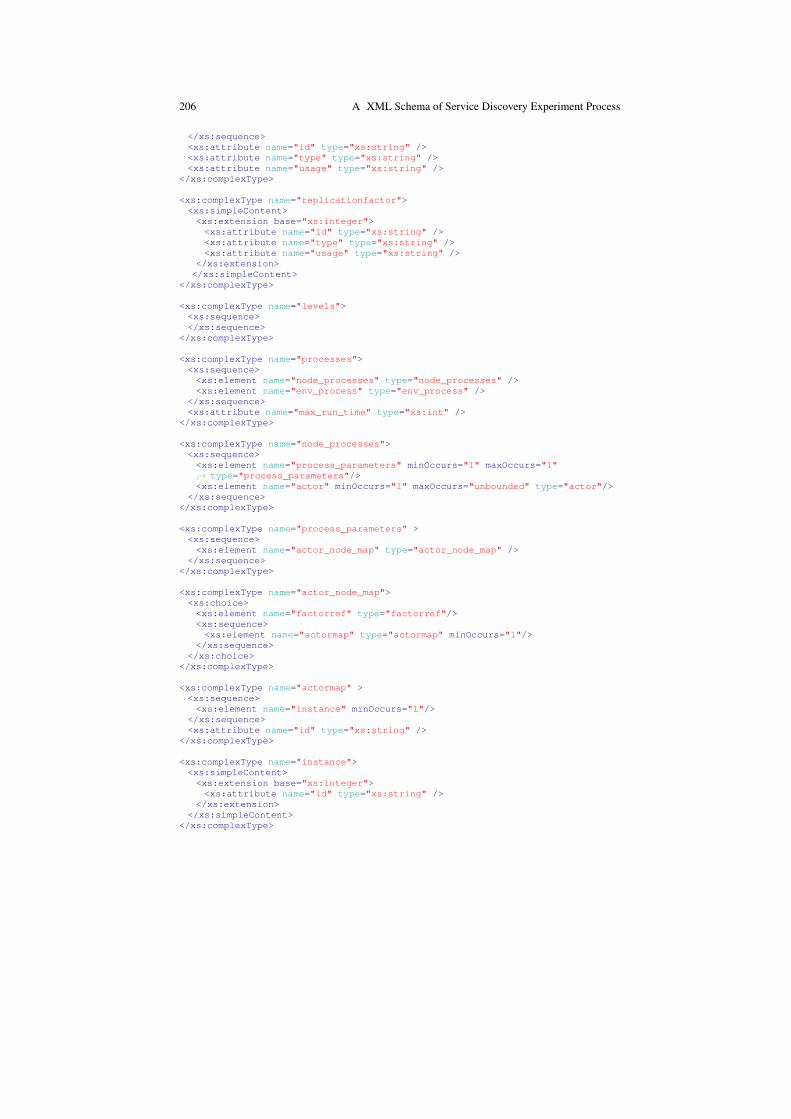
206 A XML Schema of Service Discovery Experiment Process
</xs:sequence><xs:attribute name="id" type="xs:string" /><xs:attribute name="type" type="xs:string" /><xs:attribute name="usage" type="xs:string" />
</xs:complexType>
<xs:complexType name="replicationfactor"><xs:simpleContent><xs:extension base="xs:integer"><xs:attribute name="id" type="xs:string" /><xs:attribute name="type" type="xs:string" /><xs:attribute name="usage" type="xs:string" />
</xs:extension></xs:simpleContent>
</xs:complexType>
<xs:complexType name="levels"><xs:sequence></xs:sequence>
</xs:complexType>
<xs:complexType name="processes"><xs:sequence><xs:element name="node_processes" type="node_processes" /><xs:element name="env_process" type="env_process" />
</xs:sequence><xs:attribute name="max_run_time" type="xs:int" />
</xs:complexType>
<xs:complexType name="node_processes"><xs:sequence><xs:element name="process_parameters" minOccurs="1" maxOccurs="1"↩→ type="process_parameters"/><xs:element name="actor" minOccurs="1" maxOccurs="unbounded" type="actor"/>
</xs:sequence></xs:complexType>
<xs:complexType name="process_parameters" ><xs:sequence><xs:element name="actor_node_map" type="actor_node_map" />
</xs:sequence></xs:complexType>
<xs:complexType name="actor_node_map"><xs:choice><xs:element name="factorref" type="factorref"/><xs:sequence><xs:element name="actormap" type="actormap" minOccurs="1"/>
</xs:sequence></xs:choice>
</xs:complexType>
<xs:complexType name="actormap" ><xs:sequence><xs:element name="instance" minOccurs="1"/>
</xs:sequence><xs:attribute name="id" type="xs:string" />
</xs:complexType>
<xs:complexType name="instance"><xs:simpleContent><xs:extension base="xs:integer"><xs:attribute name="id" type="xs:string" />
</xs:extension></xs:simpleContent>
</xs:complexType>

A XML Schema of Service Discovery Experiment Process 207
<xs:complexType name="description"><xs:simpleContent><xs:extension base="xs:string"></xs:extension>
</xs:simpleContent></xs:complexType>
<xs:complexType name="actor"><xs:sequence><xs:element name="sd_actions" maxOccurs="1" /><xs:element name="manipulation_actions" minOccurs="0" maxOccurs="1" />
</xs:sequence><xs:attribute name="id" type="xs:string" /><xs:attribute name="name" type="xs:string" />
</xs:complexType>
<xs:complexType name="factorref" ><xs:attribute name="id" type="xs:string" />
</xs:complexType>
<xs:complexType name="sd_actions" /><xs:complexType name="manipulation_actions" /><xs:complexType name="env_process"><xs:sequence><xs:element name="description" type="description" /><xs:element name="env_actions" type="env_actions" />
</xs:sequence></xs:complexType>
<xs:complexType name="env_actions"><xs:sequence><xs:element type="flow_control_actions" minOccurs="0" maxOccurs="unbounded"↩→ />
</xs:sequence></xs:complexType>
<xs:complexType name="flow_control_actions" /><xs:choice></xs:choice>
</xs:complexType>
<!-- ACTIONS //--><xs:complexType name="traffic"><xs:sequence><xs:element name="pairs" /><xs:element name="bw" /><xs:element name="choice" />
</xs:sequence></xs:complexType>
<xs:complexType name="wait_for_event"><xs:sequence></xs:sequence>
</xs:complexType>
</xs:schema>


Appendix BExCovery Process Description
This listing contains experiment and environment process descriptions as used forthe experiments conducted in this work. See also Chapters 6 and 3.
<!-- ... --><processes max_run_time="120"><node_processes name=""><process_parameters><actor_node_map><factorref id="fact_nodes"/>
</actor_node_map></process_parameters>
<actor id="responder" name="publisher"><sd_actions><sd_init /><sd_publish /><wait_for_event><event_dependency>done</event_dependency>
</wait_for_event><sd_unpublish /><sd_exit />
</sd_actions></actor>
<actor id="requester" name="searcher"><sd_actions><wait_for_event><from_dependency><node actor="responder" instance="all"/>
</from_dependency><event_dependency>sd_start_publish</event_dependency>
</wait_for_event><wait_for_event><event_dependency>ready_to_init</event_dependency>
</wait_for_event><sd_init /><wait_for_event><event_dependency>ready_to_search</event_dependency>
</wait_for_event><wait_marker />
<sd_start_search /><wait_for_event><from_dependency><node actor="requester" instance="all"/>
209

210 B ExCovery Process Description
</from_dependency><event_dependency>sd_service_add</event_dependency><param_dependency><node actor="responder" instance="all" />
</param_dependency><timeout>30</timeout>
</wait_for_event><event_flag><value>done</value></event_flag>
<sd_stop_search /><sd_exit />
</sd_actions></actor>
</node_processes>
<env_process><description>The sd process is treated with a varying network↩→ traffic</description><env_actions><wait_for_event><from_dependency>
<node actor="responder" instance="all"/></from_dependency><event_dependency>sd_start_publish</event_dependency>
</wait_for_event><wait_marker />
<env_start_drop_sd /><wait_time><value>5</value>
</wait_time><event_flag><value>ready_to_init</value>
</event_flag>
<env_traffic_start><bw><factorref id="fact_bw" />
</bw><choice>0</choice><random_switch_amount>1</random_switch_amount><random_switch_seed><factorref id="fact_replication_id" />
</random_switch_seed><!-- this causes the randomization in replications --><random_pairs><factorref id="fact_pairs" />
</random_pairs><random_seed><factorref id="fact_pairs"/>
</random_seed><!-- this causes the randomization in repeatitions of the same↩→ pairs-factor to be the samethis means the randomly selected nodes -->
</env_traffic_start>
<wait_for_event><from_dependency><node actor="requester" instance="all"/>
</from_dependency><event_dependency>sd_init_done</event_dependency>
</wait_for_event><wait_time><value>1</value>
</wait_time><env_stop_drop_sd />

B ExCovery Process Description 211
<event_flag><value>ready_to_search</value>
</event_flag>
<wait_for_event><event_dependency>done</event_dependency>
</wait_for_event><env_traffic_stop />
</env_actions></env_process>
</processes><!-- ... -->


Index
ExCovery, experiment framework, 41, 47experiment description, 52–62measurement and storage, 49, 161platform requirements, 48
acronyms, list of, xxi
correlation metricsPearson product-moment correlation
coefficient, 168root mean squared error, 167
experimentsdesign of, 42, 44, 162factors, 43testbed behavior, 129–135used testbeds, 110, 114, 116, 162validity, 44
failure rate, 25fault model, 32
infrastructureuser-perceived, 5, 90, 96
main contributions, 10mean time to failure, 26mean time to repair, 26
probabilistic breadth-first search, 144–147algorithm, 146validation, 148–154
problem statement, 6
reliability, 25responsiveness, 29
definition, 6, 29expected responsiveness distance, 9, 157experiment results, 120
service availability, 24, 26instantaneous, 25, 26, 86, 100interval, 26steady-state, 26, 96user-perceived, 5, 76user-perceived model generation, 81–87user-perceived model specification, 70–76
service discovery, 4, 16architectures, 18communication types, 20dependability, 30protocol retry intervals, 19protocols, 19, 21–23scenarios, 111–113, 155–159stochastic model, 138–141, 154
correlation, 166–174validation, 161
service-oriented computing, 13fault taxonomies, 24service definition, 16
UML, use in this work, 34
wireless communication, 35network-wide broadcasts, 37, 143, 145routing, 36transmission delays, 143
213