the_effect_of_flow_instability.pdf - ucl discovery
TRANSCRIPT
THE EFFECT
OF FLOW INSTABILITY ON RESIDENCE TIME DISTRIBUTION
OF NEWTONIAN AND NON-NEWTONIAN LIQUIDS
IN COUETTE-FLOW
SAMSON SAU SHUN YIM, B.ENG (Hons)
A thesis submitted for the Degree of Doctor o f Philosophy
in the University o f London
Ramsay Memorial Laboratory of Chemical Engineering Torrington Place London WCIE 7 JE
March 1997
ProQuest Number: 10017292
All rights reserved
INFORMATION TO ALL USERS The quality of this reproduction is dependent upon the quality of the copy submitted.
In the unlikely event that the author did not send a complete manuscript and there are missing pages, these will be noted. Also, if material had to be removed,
a note will indicate the deletion.
uest.
ProQuest 10017292
Published by ProQuest LLC(2016). Copyright of the Dissertation is held by the Author.
All rights reserved.This work is protected against unauthorized copying under Title 17, United States Code.
Microform Edition © ProQuest LLC.
ProQuest LLC 789 East Eisenhower Parkway
P.O. Box 1346 Ann Arbor, Ml 48106-1346
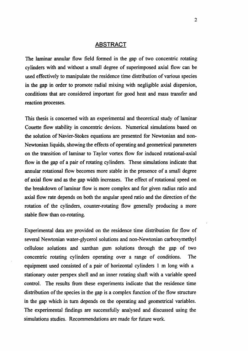
ABSTRACT
The laminar annular flow field formed in the gap of two concentric rotating
cylinders with and without a small degree of superimposed axial flow can be
used effectively to manipulate the residence time distribution of various species
in the gap in order to promote radial mixing with negligible axial dispersion,
conditions that are considered important for good heat and mass transfer and
reaction processes.
This thesis is concerned with an experimental and theoretical study of laminar
Couette flow stability in concentric devices. Numerical simulations based on
the solution of Navier-Stokes equations are presented for Newtonian and non-
Newtonian liquids, showing the effects o f operating and geometrical parameters
on the transition of laminar to Taylor vortex flow for induced rotational-axial
flow in the gap of a pair of rotating cylinders. These simulations indicate that
annular rotational flow becomes more stable in the presence o f a small degree
of axial flow and as the gap width increases. The effect o f rotational speed on
the breakdown of laminar flow is more complex and for given radius ratio and
axial flow rate depends on both the angular speed ratio and the direction of the
rotation o f the cylinders, counter-rotating flow generally producing a more
stable flow than co-rotating.
Experimental data are provided on the residence time distribution for flow of
several Newtonian water-glycerol solutions and non-Newtonian carboxymethyl
cellulose solutions and xanthan gum solutions through the gap of two
concentric rotating cylinders operating over a range of conditions. The
equipment used consisted of a pair of horizontal cylinders 1 m long with a
stationary outer perspex shell and an inner rotating shaft with a variable speed
control. The results from these experiments indicate that the residence time
distribution of the species in the gap is a complex function of the flow structure
in the gap which in turn depends on the operating and geometrical variables.
The experimental findings are successfully analysed and discussed using the
simulations studies. Recommendations are made for future work.
DEDICATION
Œb My
"Learning, oSserving, try not to stay on tHe surface o f facts.(Do not Become tfie arcBivists o f facts.
Try to penetrate to the secret o f tBeir occurrence, persistentCy search fo r the Caws which govern them. "
Ivan (Petrovich Pavlov {1849 - 1936)
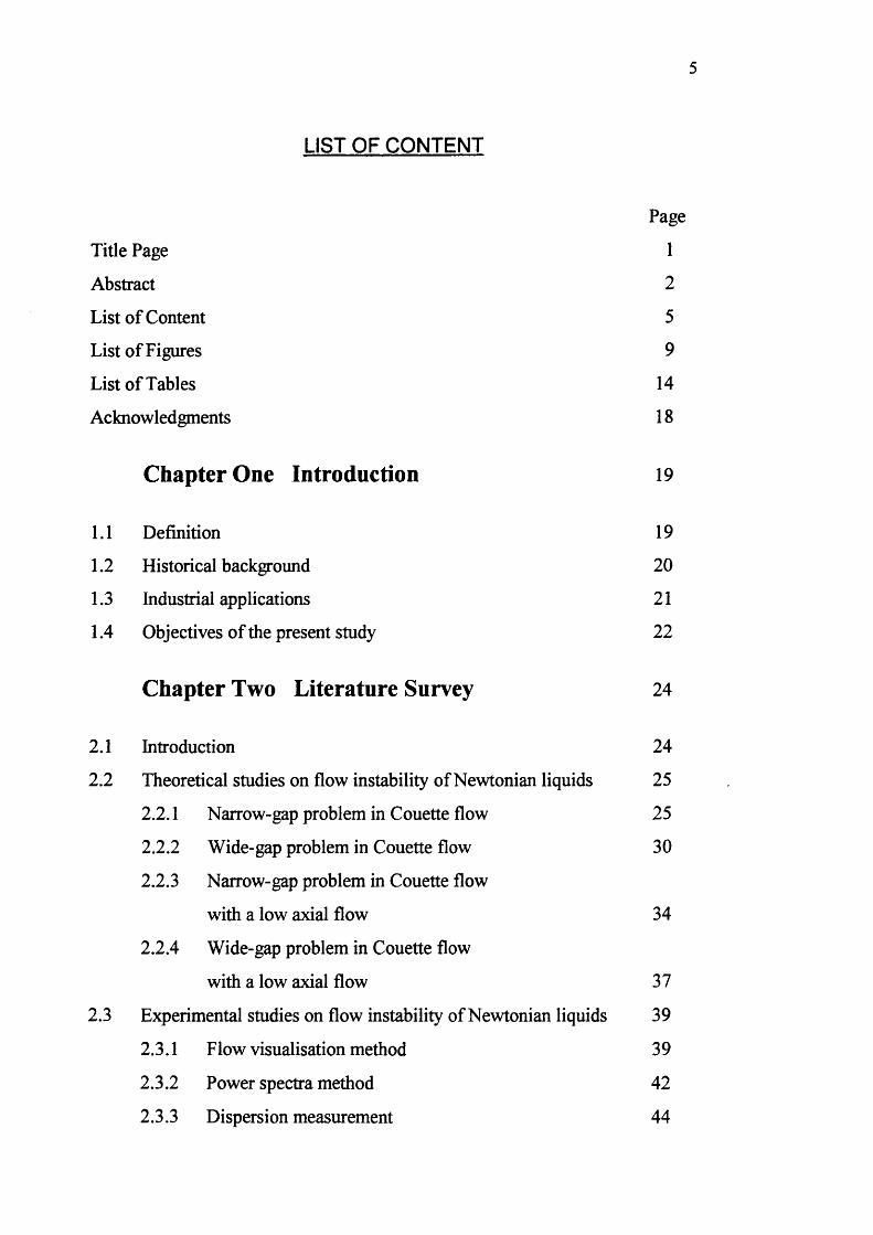
LIST OF CONTENT
Page
Title Page 1
Abstract 2
List o f Content 5
List o f Figures 9
List o f Tables 14
Acknowledgments 18
Chapter One Introduction 19
1.1 Definition 19
1.2 Historical background 20
1.3 Industrial applications 21
1.4 Objectives of the present study 22
Chapter Two Literature Survey 24
2.1 Introduction 24
2.2 Theoretical studies on flow instability of Newtonian liquids 25
2.2.1 Narrow-gap problem in Couette flow 25
2.2.2 Wide-gap problem in Couette flow 30
2.2.3 Narrow-gap problem in Couette flow
with a low axial flow 34
2.2.4 Wide-gap problem in Couette flow
with a low axial flow 37
2.3 Experimental studies on flow instability of Newtonian liquids 39
2.3.1 Flow visualisation method 39
2.3.2 Power spectra method 42
2.3.3 Dispersion measurement 44
2.4 Theoretical studies on flow instability o f non-Newtonian liquids 50
2.5 Experimental studies on flow instability of non-Newtonian liquids 51
2.6 Summary 53
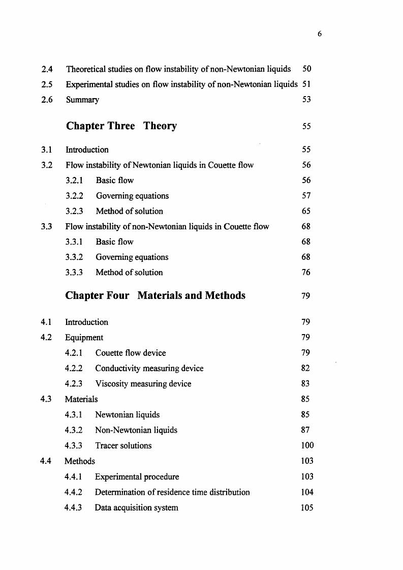
Chapter Three Theory 55
3.1 Introduction 55
3.2 Flow instability of Newtonian liquids in Couette flow 56
3.2.1 Basic flow 56
3.2.2 Governing equations 57
3.2.3 Method of solution 65
3.3 Flow instability of non-Newtonian liquids in Couette flow 68
3.3.1 Basic flow 68
3.3.2 Governing equations 68
3.3.3 Method of solution 76
Chapter Four Materials and Methods 79
4.1 Introduction 79
4.2 Equipment 79
4.2.1 Couette flow device 79
4.2.2 Conductivity measuring device 82
4.2.3 Viscosity measuring device 83
4.3 Materials 85
4.3.1 Newtonian liquids 85
4.3.2 Non-Newtonian liquids 87
4.3.3 Tracer solutions 100
4.4 Methods 103
4.4.1 Experimental procedure 103
4.4.2 Determination o f residence time distribution 104
4.4.3 Data acquisition system 105
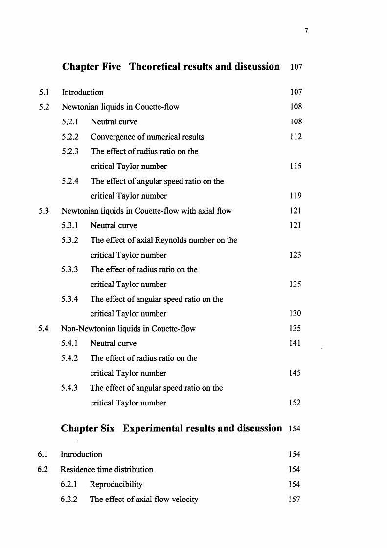
Chapter Five Theoretical results and discussion 107
5.1 Introduction 107
5.2 Newtonian liquids in Couette-flow 108
5.2.1 Neutral curve 108
5.2.2 Convergence o f numerical results 112
5.2.3 The effect o f radius ratio on the
critical T ay lor number 115
5.2.4 The effect o f angular speed ratio on the
critical Taylor number 119
5.3 Newtonian liquids in Couette-flow with axial flow 121
5.3.1 Neutral curve 121
5.3.2 The effect o f axial Reynolds number on the
critical Taylor number 123
5.3.3 The effect o f radius ratio on the
critical Taylor number 125
5.3.4 The effect o f angular speed ratio on the
critical Taylor number 130
5.4 Non-Newtonian liquids in Couette-flow 135
5.4.1 Neutral curve 141
5.4.2 The effect of radius ratio on the
critical Taylor number 145
5.4.3 The effect o f angular speed ratio on the
critical Taylor number 152
Chapter Six Experimental results and discussion 154
6.1 Introduction 154
6.2 Residence time distribution 154
6.2.1 Reproducibility 154
6.2.2 The effect o f axial flow velocity 157
6.2.3 The effect o f rotational speed 157
6.2.4 The effect o f electrode positions 165
6.3 Axial dispersion in Couette flow 168
6.3.1 Axial dispersion model 168
6.3.2 Peclet number 173
6.3.3 The effect o f inner cylinder geometry 197
6.4 Comparison of theoretical and experimental results 201
Chapter Seven Conclusions and Recommendations 205
7.1 Conclusions 205
7.2 Recommendations for further work 208
Nomenclature 210
References 214
Appendix 1 Galerkin Method 222
Appendix 2 Mathematica program for flow instability of
Newtonian liquids in Couette flow 224
Appendix 3 Mathematica program for flow instability of
non-Newtonian liquids in Couette flow 233
Appendix 4 Computer program for conductivity measurement
and control system 239
Appendix 5 Sample calculations of Peclet number from
experimental RTD data 245
Appendix 6 Published papers relating to this project 248
LIST OF FIGURES
page
Figure 2.1 Hydrodynamics of Couette flow 26
Figure 2.2 Taylor vortices 26
Figure 3.1 Annulus configuration and co-ordinate system 56
Figure 4.1 Experimental set-up 80
Figure 4.2 Inner cylinder shaft (with blades) 81
Figure 4.3 Conductivity probe 82
Figure 4.4 Viscometer 84
Figure 4.5 Shear stress-shear rate plot for different concentration
of Newtonian glycerol-water solutions 86
Figure 4.6 Classes of non-Newtonian behaviour 88
Figure 4.7 Typical logarithmic plot o f a non-Newtonian liquid 88
Figure 4.8 Shear stress-shear rate plot for different concentration
of non-Newtonian carboxymethyl cellulose solutions 93
Figure 4.9 Logarithmic shear stress-shear rate plot for different
concentration o f non-Newtonian carboxymethyl
cellulose solutions 94
Figure 4.10 Shear stress-shear rate plot for different concentration
of non-Newtonian xanthan gum solutions 95
Figure 4.11 Logarithmic shear stress-shear rate plot for different
concentration of non-Newtonian xanthan gum solutions 96
Figure 4.12 Concentration and rheology of non-Newtonian
carboxymethyl cellulose solutions 97
Figure 4.13 Concentration and rheology of non-Newtonian
xanthan gum solutions 98
Figure 4.14 Conductivity vs concentration of KCl solution 101
Figure 4.15 The influence of the amount of tracer injected
on the dimensionless RTD 102
Figure 4.16 Data acquisition system 106
10
Figure 5.1 Typical neutral curve in the Ta - A, plane 110
Figure 5.2 Neutral curve in the Ta - A. plane at different radius ratios 111
Figure 5.3 Convergence of neutral curve 114
Figure 5.4 Comparison of critical Taylor number with previous workers
on different radius ratios, a 116
Figure 5.5 The effect o f radius ratio on dimensionless wave number 118
Figure 5.6 The effect of radius ratio on critical Taylor number for
different cases of angular speed ratio 120
Figure 5.7 The effect o f dimensionless wave number, A., on Imaginaiy
part o f Taylor number Im[Ta] for different cases of
dimensionless disturbance growth rate, a 122
Figure 5.8 The effect o f radius ratio on critical Taylor number for
different cases of axial Reynolds number 126
Figure 5.9 The effect of axial Reynolds number on critical Taylor
number for different cases of angular speed ratio 129
Figure 5.10 Angular speed distribution for a range of flow index, n,
at different radial co-ordinates 137
Figure 5.10 Stress distribution for a range of flow index, n, at
different radial co-ordinates 138
Figure 5.12 Apparent viscosity for a range of flow index, n, at
different inner cylinder rotational speeds 139
Figure 5.13 Mean viscosity for a range of flow index, n, at different
inner cylinder rotational speeds 140
Figure 5.14 Neutral curves for a range of flow index 142
Figure 5.15 The effect of radius ratio on the critical Taylor number 143
Figure 5.16 The effect of flow index on the critical Taylor number 144
Figure 5.17 The effect of angular speed ratio on the critical
Taylor number 153
11
Figure 6.1 Reproducibility o f RTD experiments for Newtonian liquid 155
Figure 6.2 Reproducibility o f RTD experiments for
non-Newtonian liquid 156
Figure 6.3 RTD experiments at different axial flow velocities
for Newtonian liquid 15 8
Figure 6.4 RTD experiments at different axial flow velocities
for non-Newtonian liquid (0.6wt% xanthan gum solution) 159
Figure 6.5 RTD experiments at different rotational speeds
for Newtonian liquid (Ta < Ta ) 161
Figure 6.6 RTD experiments at different axial flow velocities
for Newtonian liquid (Ta > Tac) 162
Figure 6.7 RTD experiments at different rotational speeds
for non-Newtonian liquid (Ta < Tac)
(0.6wt% xanthan gum solution) 163
Figure 6.8 RTD experiments at different axial flow velocities
for non-Newtonian liquid (Ta > Tac)
(0.6wt% xanthan gum solution) 164
Figure 6.9 Influence of the position o f the sensor in the annular gap 165
Figure 6.10 Influence of the location of the sensor in the annular gap 165
Figure 6.11 RTD experiment at different positions of the sensor
(Newtonian liquid) 166
Figure 6.12 RTD experiments at different locations of the sensor
(Newtonian liquid) 167
Figure 6.13 Axial dispersion model 170
Figure 6.14 Comparison of axial dispersion model and the
experimental data (Newtonian liquid) 171
Figure 6.15 Comparison of axial dispersion model and the
experimental data (non-Newtonian liquid) 172
Figure 6.16 The effect of rotational speed of inner cylinder on
dimensionless variance difference of the tracer RTD curve 174
12
Figure 6.17 The effect o f Taylor number on Peclet number for
Newtonian liquid (a = 0.84, 1 < Re < 3) 176
Figure 6.18 The effect o f Taylor number on Peclet number for
Newtonian liquid (a = 0.84, 8 < Re < 27) 177
Figure 6.19 The effect o f Taylor number on Peclet number for
Newtonian liquid (a = 0.84, 35 < Re < 62) 178
Figure 6.20 The effect o f Taylor number on Peclet number for
Newtonian liquid (a = 0.67, 1 < Re < 4) 179
Figure 6.21 The effect o f Taylor number on Peclet number for
Newtonian liquid (a = 0.67, 7 < Re < 29) 180
Figure 6.22 The effect o f Taylor number on Peclet number for
Newtonian liquid (a = 0.67, 47 < Re < 69) 181
Figure 6.23 The effect of Taylor number on Peclet number for
non-Newtonian liquid (a = 0.84, 0.1 - 0.5 wt%) 182
Figure 6.24 The effect o f Taylor number on Peclet number for
non-Newtonian liquid (a = 0.84, 0.6 - 0.9 wt%) 183
Figure 6.25 The effect o f Taylor number on Peclet number for
non-Newtonian liquid (a = 0.67, 0.1 - 0.5 wt%) 184
Figure 6.26 The effect o f Taylor number on Peclet number for
non-Newtonian liquid (a = 0.67, 0.6 - 0.9 wt%) 185
Figure 6.27 The effect o f Taylor number on Peclet number for
non-Newtonian liquid (a = 0.84, 0.1 - 0.5 wt%) 186
Figure 6.28 The effect o f Taylor number on Peclet number for
non-Newtonian liquid (a = 0.84, 0.6 - 0.9 wt%) 187
Figure 6.29 The effect o f Taylor number on Peclet number for
non-Newtonian liquid (a = 0.67, 0.1 - 0.5 wt%) 188
Figure 6.30 The effect o f Taylor number on Peclet number for
non-Newtonian liquid (a = 0.67, 0.6 - 0.9 wt%) 189
13
Figure 6.31 The effect o f axial Reynolds number on critical
Taylor number at different radius ratios, a 192
Figure 6.32 The effect o f flow index on critical Taylor number
at different radius ratios, a 196
Figure 6.33 The influence of inner shaft geometry 197
Figure 6.34 The effect o f Taylor number on Peclet number
for Newtonian liquids (Shaft SI) 199
Figure 6.35 The effect o f Taylor number on Peclet number
for Newtonian liquids (Shaft S2) 200
Figure 6.36 Comparison of theoretical and experimental results
for Newtonian liquids 203
Figure 6.37 Comparison of theoretical and experimental results
for non-Newtonian liquids 204
14
LIST OF TABLES
page
Table 2.1 Summary of narrow-gap problem in Couette flow 30
Table 2.2 Summary of critical Taylor number for
different values of radius ratio 32
Table 2.3 Summaiy o f wide-gap problem in Couette flow 33
Table 2.4 Summary of narrow-gap problem in Couette flow
with axial flow 36
Table 2.5 Summary of critical Ta number for different values of
radius ratio, a and given values o f Re number 38
Table 2.6 Summary o f wide-gap problem in Couette flow
with axial flow 39
Table 2.7 Summary of major experiments on flow visualisation
method in Couette flow device 41
Table 2.8 Summary o f major experiments on power spectra
method in Couette flow device 43
Table 2.9 Summary of major experiments on dispersion
measurement in Couette flow device 49
Table 2.10 Summary of theoretical studies of non-Newtonian liquids
in Couette flow device 52
Table 2.11 Summary of experimental studies of non-Newtonian liquids
in Couette flow device 52
Table 4.1 The concentration and rheology of glycerol-water solutions 85
Table 4.2 The concentration and rheology of carboxymethyl
cellulose (CMC) solutions 99
Table 4.3 The concentration and rheology of xanthan gum solutions 99
Table 5.1 Comparison of Ta value in narrow gap geometry 112
Table 5.2 The critical Taylor number and critical dimensionless wave
number with a resting outer cylinder (p=0) as a function
of the radius ratio, a 117
15
Table 5.3 The critical Taylor number with a different angular
speed ratio, p,as a function of the radius ratio, a 119
Table 5.4 Critical Taylor number and corresponding values o f X
and G for given values of Re when a = 0.95 and (3=0 124
Table 5.5 Critical Taylor number and corresponding values o f X
and G for given values of Re when a = 0.9 and (3=0 125
Table 5.6 Critical Taylor number and corresponding values of X
and G for given values of Re when a = 0.8 and (3=0 127
Table 5.7 Critical Taylor number and corresponding values o f X
and G for given values of Re when a = 0.7 and (3=0 127
Table 5.8 Critical Taylor number and corresponding values of X
and G for given values of Re when a = 0.6 and (3=0 128
Table 5.9 Critical Taylor number and corresponding values of X
and G for given values of Re when a = 0.5 and P = 0 128
Table 5.10 Critical Taylor number and corresponding values o f X
and G for given values of Re when a = 0.4 and p = 0 130
Table 5.11 Critical Taylor number and corresponding values o f X
and G for given values of Re when a = 0.8 and P = -0.25 131
Table 5.12 Critical Taylor number and corresponding values o f X
and G for given values of Re when a = 0.6 and P = -0.25 131
Table 5.13 Critical Taylor number and corresponding values o f X
and G for given values of Re when a = 0.4 and P = -0.25 131
Table 5.14 Critical Taylor number and corresponding values of X
and G for given values o f Re when a = 0.8 and p = 0 132
Table 5.15 Critical Taylor number and corresponding values of X
and G for given values o f Re when a = 0.6 and P = 0 132
Table 5.16 Critical Taylor number and corresponding values of X
and G for given values of Re when a = 0.4 and p = 0 132
16
Table 5.17 Critical Taylor number and corresponding values o f X
and a for given values of Re when a = 0.8 and P = 0.25 133
Table 5.18 Critical Taylor number and corresponding values o f X
and a for given values of Re when a = 0.6 and P = 0.25 133
Table 5.19 Critical Taylor number and corresponding values o f X
and a for given values of Re when a = 0.4 and p = 0.25 133
Table 5.20 Critical Taylor number and corresponding values o f X
and a for given values of Re when a = 0.8 and P = 0.5 134
Table 5.21 Critical Taylor number and corresponding values o f X
and a for given values of Re when a = 0.6 and P = 0.5 134
Table 5.22 Critical Taylor number and corresponding values o f X
and a for given values of Re when a = 0.4 and p = 0.5 134
Table 5.23 Critical Taylor number for given values o f flow index
and radius ratio when angular speed ratio p = 1 146
Table 5.24 Critical dimensionless wave number for given values of
flow index and radius ratio when angular speed ratio P = 1 146
Table 5.25 Critical Taylor number for given values o f flow index
and radius ratio when angular speed ratio p = 0.5 147
Table 5.26 Critical dimensionless wave number for given values
of flow index and radius ratio when angular
speed ratio P = 0.5 147
Table 5.27 Critical Taylor number for given values o f flow index
and radius ratio when angular speed ratio p = 0.25 148
Table 5.28 Critical dimensionless wave number for given values
of flow index and radius ratio when angular
speed ratio p = 0.25 148
Table 5.29 Critical Taylor number for given values of flow index
and radius ratio when angular speed ratio p = 0 149
17
Table 5.30 Critical dimensionless wave number for given values
o f flow index and radius ratio when angular
speed ratio P = 0
Table 5.31 Critical Taylor number for given values o f flow index
and radius ratio when angular speed ratio p = -0.25
Table 5.32 Critical dimensionless wave number for given values
o f flow index and radius ratio when angular
speed ratio p = -0.25
Table 5.33 Critical Taylor number for given values of flow index
and radius ratio when angular speed ratio P = -0.5
Table 5.34 Critical dimensionless wave number for given values
o f flow index and radius ratio when angular
speed ratio p = -0.5
Table 6.1 Summary of the experimental Pe - Ta plots
Table 6.2 Experimental results o f Tac for Newtonian glycerol
solutions (a = 0.84)
Table 6.3 Experimental results of Tac for Newtonian glycerol
solutions (a = 0.67)
Table 6.4 Experimental results o f Tac for non-Newtonian
solutions (a = 0.84)
Table 6.5 Experimental results o f Tac for non-Newtonian
solutions (a = 0.67)
Table 6.6 The specifications of different inner rotating cylinder
geometry
149
150
150
151
151
175
190
191
193
194
197
18
ACKNOWLEDGMENTS
The author would first like to acknowledge, with sincere gratitude, the
invaluable assistance, guidance, and encouragement of his supervisor. Dr. P.
Ayazi Shamlou who has given generously of his time and wise counsel during
the period of this work.
Successful operation of the stability apparatus would not have been possible
without the support of the technical staff for which the author is eternally
grateful. Gratitude is owed to Martin Town, Martyn Vale, Samuel Okagbue,
Carol Welfare and Julian Perfect for contributing the equipment and
experimental materials used in his investigation. The author also likes to thank
all his colleagues, past, and present, for providing a fiiendly and humorous
working environment.
This study could not have taken off had it not been for the inspirational,
dedicated and supportive attitude of his dear wife, Mei-Yee. Besides, the
author would like to express his deep gratitude to his parents for their
encouragement and support at all times.
The author is deeply indebted to many individuals who have contributed to the
successful completion of this work.
Finally, the author gratefully acknowledge the financial support of the
Croucher Foundation Scholarships and the Overseas Research Students Award
Scheme.
Introduction 19
CHAPTER ONE
INTRODUCTION
1.1 Definition
The production and processing of Newtonian and non-Newtonian materials
frequently involve the flow of material through concentric cylinder flow
devices and often several unit operations can occur concurrently during flow.
These unit operations include heat transfer, mixing, émulsification, dispersion,
crystallisation and chemical reaction. The Couette flow device basically
consists of a pair of concentric rotating cylinders in which the outer shell may
be jacketed to facilitate heat transfer through its wall. In this way the
temperature of the process material can be controlled as it flows through the
annular gap between the two cylinders. In the food industry, in the case of
margarine and ice-cream for example, heat transfer to the process material
during flow causes crystallisation of fat and brings about significant changes in
the rheological properties o f the final product.
Most of the unit operations that occur in a Couette flow device are affected by
the behaviour of the material during flow and in the case of steady state
continuous processes a key factor is the variation in the duration of stay within
the process equipment experienced by "particles" which entered the equipment
at the same time. This variation is normally expressed in terms o f the residence
time distribution (RTD) and as a result measurement and analysis of RTD has
become an important tool in the study of continuous processes. Understanding
the relationship between the fluid dynamics and the RTD in a Couette flow
device is therefore of basic research interest to academics and industrialists.
Introduction 20
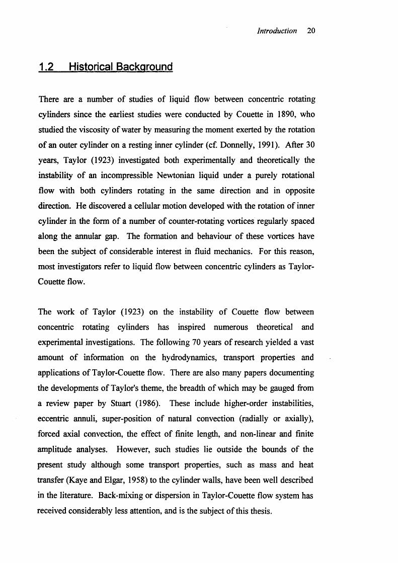
1.2 Historical Background
There are a number of studies of liquid flow between concentric rotating
cylinders since the earliest studies were conducted by Couette in 1890, who
studied the viscosity of water by measuring the moment exerted by the rotation
o f an outer cylinder on a resting inner cylinder (cf. Donnelly, 1991). After 30
years, Taylor (1923) investigated both experimentally and theoretically the
instability o f an incompressible Newtonian liquid under a purely rotational
flow with both cylinders rotating in the same direction and in opposite
direction. He discovered a cellular motion developed with the rotation of inner
cylinder in the form of a number of counter-rotating vortices regularly spaced
along the annular gap. The formation and behaviour of these vortices have
been the subject of considerable interest in fluid mechanics. For this reason,
most investigators refer to liquid flow between concentric cylinders as Taylor-
Couette flow.
The work o f Taylor (1923) on the instability o f Couette flow between
concentric rotating cylinders has inspired numerous theoretical and
experimental investigations. The following 70 years o f research yielded a vast
amount o f information on the hydrodynamics, transport properties and
applications of Taylor-Couette flow. There are also many papers documenting
the developments o f Taylor's theme, the breadth of which may be gauged from
a review paper by Stuart (1986). These include higher-order instabilities,
eccentric annuli, super-position of natural convection (radially or axially),
forced axial convection, the effect of finite length, and non-linear and finite
amplitude analyses. However, such studies lie outside the bounds of the
present study although some transport properties, such as mass and heat
transfer (Kaye and Elgar, 1958) to the cylinder walls, have been well described
in the literature. Back-mixing or dispersion in Taylor-Couette flow system has
received considerably less attention, and is the subject of this thesis.
Introduction 21
1.3 Industrial Applications
In many industrial processing situations, from polymer processing to paper-
making, from foods to pharmaceuticals and from chemical to biochemical it is
often desirable to generate plug flow of processing liquids, in order to
maximise the driving force for transfer processes, for example. The defmition
of "plug flow" is given by Levenspiel (1972) as the flow o f liquid through the
equipment is orderly with no element of liquid overtaking or mixing with any
other element ahead or behind but there may be lateral mixing of liquid in a
plug flow equipment.
Most industrially important liquids are non-Newtonian and develop a wide
residence time distribution (RTD) in pipe flow which makes the mass and heat
transfer difficult to control. For example, polymerisation is a particularly
important class of reactions in which deviation from plug flow is
disadvantageous and difficult to prevent because of the variable apparent
viscosity of the liquid at different shear rate across the reactor. In this case, the
added degree of freedom obtained by rotating the inner cylinder or a continuous
Couette flow device means that a relatively narrow RTD may be achieved even
for high viscosity liquids. Moreover, in polymerisation reactions, another
difficulty that is frequently experienced is the deposition of very high
molecular weight solid on the inner wall o f the equipment. The unique local
radial liquid flow of Taylor-Couette flow, induced by the inner rotating
cylinder, often causes a reduction in the deposition.
There is a number of publications on the hydrodynamics, transport properties
and applications of the Couette flow device. Some practical applications
presented over the years include catalytic chemical reactors (Cohen and Maron,
1983), dynamics filtration and classification on a cylindrical surface (Tobler,
1982; Rushton and Zhang, 1988), blood plasmaphoresis devices (Beaudoin and
Introduction 22
Jaffiin, 1989), characterisation of shear-dependent rate processes as in
agglomeration and breakage of particles formed during precipitation processes
(Hoare, et al., 1982), cooling of rotating electrical machinery (Kaye and Elgar,
1958), ice crystallisation (Wey and Bstrin, 1973), electrolytic applications
(Legrand and Coeuret, 1986), offshore oil exploitation (Rosant, 1994).
1.4 Objectives of the Present Study
The objective of this work is to mathematically study and experimentally
describe the dependence of the RTD in a Couette flow device on some o f the
important of operating and material variables. Both Newtonian and non-
Newtonian liquids will be used in the experiments.
It is believed that dispersion is an important factor in Couette flow devices as
the amount of mixing in different flow regimes greatly influences the
productivity of a reactive system (Cohen and Maron, 1983). Design, scale-up
and optimisation calculations for Couette flow devices require an understanding
of the transport properties o f Taylor-Couette flow. Moreover, the stability of
flow o f non-Newtonian liquids with variable viscosity has not so far been taken
into consideration. These provided the motivation for the present study.
The theoretical section of the present study has been devoted to the treatment of
the Couette flow instability of both Newtonian and non-Newtonian liquids.
The theoretical prediction of Newtonian liquids in Couette flow has been
developed for many years as discussed later in the Section 2.2. In this
investigation, a more general Couette flow problem will be proposed to include
operational and geometrical factors and the addition of axial flow velocity. In
the case of non-Newtonian liquids, effects such as flow index, consistency
index may influence the criterion of flow instability which are different form
Introduction 23
the Newtonian case. For the system investigated, the onset o f flow instability,
defined as critical Taylor numbers, are presented as functions o f rheological
properties o f the liquid medium, operational and geometrical properties o f the
Couette flow device.
Experimental considerations have also been given in the thesis to the RTD of a
range of Newtonian glycerol water solutions and two non-Newtonian liquids
(carboxymethyl cellulose solutions and xanthan gum solutions). A stimulus
response experimental technique based on an impulse input is employed. The
experimental results are interpreted in terms of a single parameter axial
dispersion model. The data include results from experiments in which flow
transition occurred from laminar to Taylor Couette flow regime. Finally, the
findings from these experiments are analysed and assessed using the
simulations studies.
Literature Survey 24
CHAPTER TWO
LITERATURE SURVEY
2.1 Introduction
In this chapter, an overview of literature survey o f flow instability study in
Couette flow will be given both theoretically and experimentally. Section 2.2
covers the theoretical development of flow instability problem in Couette flow.
Special attention will be given to Newtonian liquids. This section will be
subdivided into four parts:
1) Narrow-gap problem in Couette flow
2) Wide-gap problem in Couette flow
3) Narrow-gap problem in Couette flow with a low axial flow
4) Wide-gap problem in Couette flow with a low axial flow
In Section 2.3, the experimental studies of flow instability of a Newtonian
liquid will be discussed. Again, this section will be subdivided into three parts:
1) Flow visualisation method
2) Power spectra method
3) Dispersion measurement
The theoretical and experimental studies on the flow instability o f non-
Newtonian liquids will be discussed in Section 2.4 and 2.5 respectively.
Finally in Section 2.6, general comments on the problem of flow instability in a
Couette flow device will be given. The major studies will be summarised at the
end o f each subsection.
Literature Survey 25
2.2 Theoretical Studies on Flow Instability of
Newtonian Liquids
2.2.1 Narrow-aap problem in Couette flow
Lord Rayleigh (1916) first considered the instability o f liquid flow between two
long concentric rotating cylinders for an inviscid liquid. He derived a simple
condition for instability with respect to rotational disturbances based on energy
consideration. He assumed that, in real liquids, viscosity served to maintain the
steady flow but did not affect the occurrence o f instability. Rayleigh’s criterion
led the conclusion that, for cylinders rotating in the same direction, flow was
stable if OiRi^ > QiRi^, where and O2 were the angular velocities of the
inner and outer cylinder respectively, Ri and R2 were the corresponding radii.
In 1923, Taylor (1923) made a brilliant contribution to the theory of
hydrodynamic stability by quantitatively predicting the flow instability of a
Newtonian liquid flowing between a pair of concentric rotating cylinders. He
stated that for very low rotational speeds of the inner cylinder, the liquid simply
moved azimuthally around the cylinders (see Figure 2.1). The radial pressure
gradient o f the liquid was responsible for the centripetal acceleration that kept
the liquid moving in circular paths. If, however, a ring of liquid was perturbed
outward to a larger radius, the local pressure gradient might not be sufficient to
restore the liquid to its original path. If instability occurred, the liquid
continued to be ejected outward until it met the outer cylinder; here the liquids
forced to overturn and, hence, travelled in the helical paths that constitute
toroidal vortices, now known as Taylor vortices, spaced regularly along the
cylindrical axis (see Figure 2.2).
Literature Survey 26
Ceniiifiigal force (ky rptation of inner cylinder)
Centripetal force \^ y pressure gradient of the liquid)!
Outer cylinder
A ring of liquidLiner cylinder
Figure 2.1 Hydrodynamics of Couette flow
A pair of Taylor vortices/ \
Rotating inner cyiinder
Annular gap
Stainless steel
Perspex outer cylinder
Figure 2.2 Taylor vortices
Literature Survey 27
Taylor (1923) began by assuming that, superimposed upon the Couette motion,
there was a small secondary velocity perturbation which was a function of the
radial and axial coordinate. He employed this assumption in the Navier-Stokes
and continuity equations, dropped those terms involving products o f secondary
quantities, and obtained a set of "disturbance equations" which were linear and
homogeneous in the component of main Couette flow. When combined with
the homogeneous boundary conditions on small secondary velocity
perturbation, these disturbance equations defined an "eigenvalue problem" for
the angular velocity o f the inner cylinder. The minimum value of angular
velocity, over all allowable eigenvectors then gave the critical conditions for
the onset o f instability. The solution of the eigenvalue problem was expressed
in term of Bessel function formula. In order to reduce the numerical difficulties
originating from the sum of the Bessel functions he made the so-called narrow-
gap approximation, which meant that he assumed the annular gap between the
cylinders was much smaller than the inner cylinder. So that, the Bessel
functions were replaced by the trigonometrical functions. After laborious
calculations he arrived at an equation for the critical condition for instability as
a function of the rotational speed of the cylinders, the radii o f the cylinders, and
the viscosity of the liquid. From his calculations, Taylor found that the
criterion for the onset o f instability could be expressed in the following form:
Onset o f instability = -------- ?------------7t [l + b /2R i] -------------------- p ] ]0.0571 [1 + 0.652 b/RiJ + 0.00056 [l + 0.652 b / Ri l
where b corresponds to the annular gap width and Ri corresponds to the radius
of inner cylinder. By using the small-gap approximation assumption, he
determined a dimensionless parameter defined in terms of geometrical and
operational factors, which was later defined as the Taylor number. Ta. The
minimum eigenvalue interpreting the onset of instability, defined as critical
Taylor number, Ta , was found approximately to be 1700. According to
Taylor's linear theory, for values of the speed of rotation less than the critical
Literature Survey 28
speed all disturbances o f the flow in the annulus were damped owing to the
action o f viscosity, whereas for speeds greater than the critical speed, some of
disturbances would be amplified with increasing time and the flow would
become unstable with the formation of a steady secondary flow in the form of
pairs o f counter-rotating vortices. Taylor’s theoretical calculations were
verified convincingly by his own laboratory experiments, which showed that,
with the inner cylinder rotating and the outer cylinder at rest, the instability of
laminar Couette flow led to the Taylor-Couette flow in which a secondary
motion with cellular toroidal vortices appeared regularly in the axial direction.
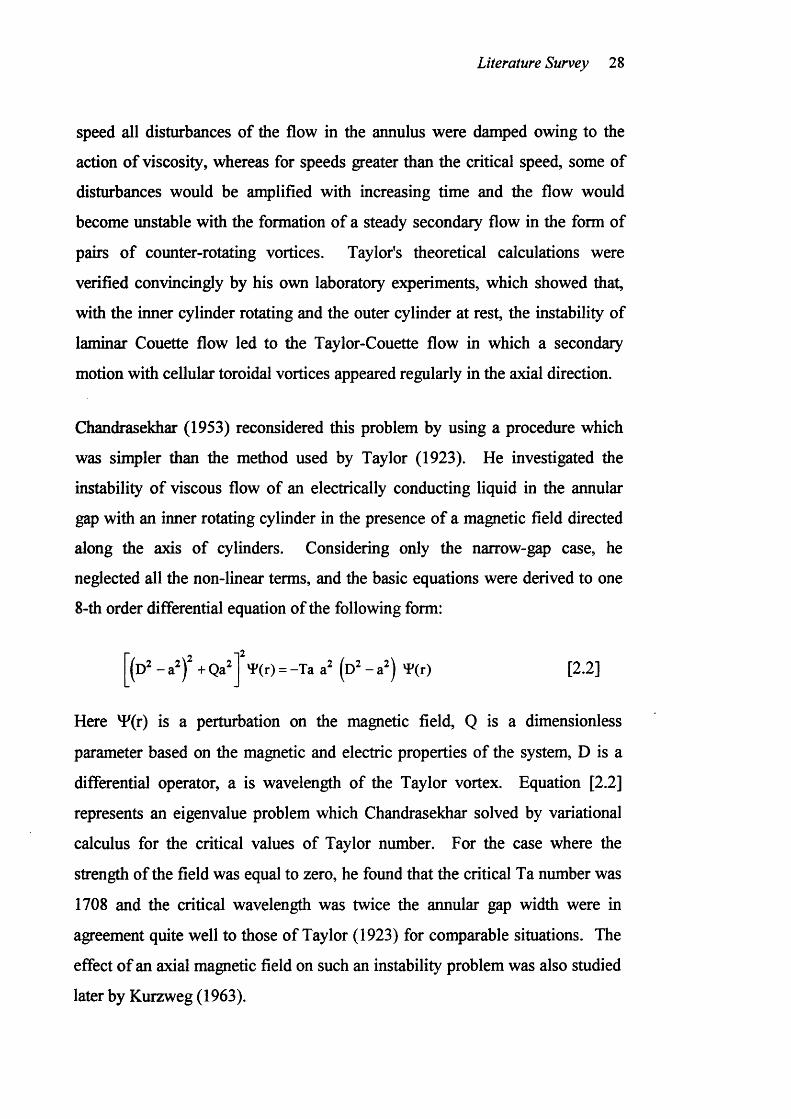
Chandrasekhar (1953) reconsidered this problem by using a procedure which
was simpler than the method used by Taylor (1923). He investigated the
instability o f viscous flow of an electrically conducting liquid in the annular
gap with an inner rotating cylinder in the presence o f a magnetic field directed
along the axis o f cylinders. Considering only the narrow-gap case, he
neglected all the non-linear terms, and the basic equations were derived to one
8-th order differential equation of the following form:
-]2(d - afjf + Qa Y(r) = -Ta a' (d - a ) T(r) [2.2]
Here 'T(r) is a perturbation on the magnetic field, Q is a dimensionless
parameter based on the magnetic and electric properties o f the system, D is a
differential operator, a is wavelength of the Taylor vortex. Equation [2.2]
represents an eigenvalue problem which Chandrasekhar solved by variational
calculus for the critical values of Taylor number. For the case where the
strength of the field was equal to zero, he found that the critical Ta number was
1708 and the critical wavelength was twice the annular gap width were in
agreement quite well to those of Taylor (1923) for comparable situations. The
effect o f an axial magnetic field on such an instability problem was also studied
later by Kurzweg (1963).
Literature Survey 29
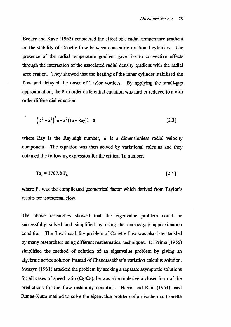
Becker and Kaye (1962) considered the effect o f a radial temperature gradient
on the stability o f Couette flow between concentric rotational cylinders. The
presence of the radial temperature gradient gave rise to convective effects
through the interaction o f the associated radial density gradient with the radial
acceleration. They showed that the heating of the inner cylinder stabilised the
flow and delayed the onset o f Taylor vortices. By applying the small-gap
approximation, the 8-th order differential equation was further reduced to a 6-th
order differential equation.
û + a^(Ta-Ray)û = 0 [2.3]
where Ray is the Rayleigh number, û is a dimensionless radial velocity
component. The equation was then solved by variational calculus and they
obtained the following expression for the critical Ta number.
Tac= 1707.8 Fg [2.4]
where Fg was the complicated geometrical factor which derived from Taylor’s
results for isothermal flow.
The above researches showed that the eigenvalue problem could be
successfully solved and simplified by using the narrow-gap approximation
condition. The flow instability problem of Couette flow was also later tackled
by many researchers using different mathematical techniques. Di Prima (1955)
simplified the method of solution of an eigenvalue problem by giving an
algebraic series solution instead of Chandrasekhar’s variation calculus solution.
Meksyn (1961) attacked the problem by seeking a separate asymptotic solutions
for all cases o f speed ratio (Ü2/f^i), he was able to derive a closer form o f the
predictions for the flow instability condition. Harris and Reid (1964) used
Runge-Kutta method to solve the eigenvalue problem of an isothermal Couette
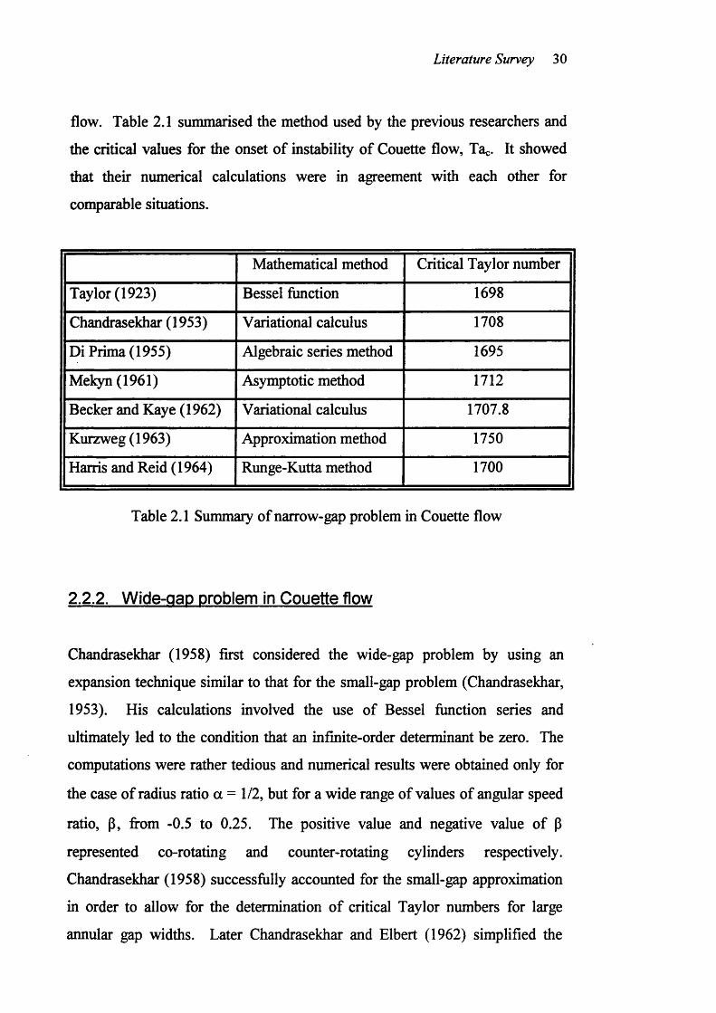
Literature Survey 30
flow. Table 2.1 summarised the method used by the previous researchers and
the critical values for the onset o f instability of Couette flow, Ta . It showed
that their numerical calculations were in agreement with each other for
comparable situations.
Mathematical method Critical Taylor number
Taylor (1923) Bessel function 1698
Chandrasekhar ( 1953) Variational calculus 1708
Di Prima (1955) Algebraic series method 1695
Mekyn (1961) Asymptotic method 1712
Becker and Kaye (1962) Variational calculus 1707.8
Kurzweg (1963) Approximation method 1750
Harris and Reid (1964) Runge-Kutta method 1700
Table 2.1 Summary of narrow-gap problem in Couette flow
2.2.2. Wide-gap problem in Couette flow
Chandrasekhar (1958) first considered the wide-gap problem by using an
expansion technique similar to that for the small-gap problem (Chandrasekhar,
1953). His calculations involved the use of Bessel function series and
ultimately led to the condition that an infinite-order determinant be zero. The
computations were rather tedious and numerical results were obtained only for
the case o f radius ratio a = 1/2, but for a wide range of values of angular speed
ratio, p, from -0.5 to 0.25. The positive value and negative value of p
represented co-rotating and counter-rotating cylinders respectively.
Chandrasekhar (1958) successfully accounted for the small-gap approximation
in order to allow for the determination of critical Taylor numbers for large
annular gap widths. Later Chandrasekhar and Elbert (1962) simplified the
Literature Survey 31
annular gap widths. Later Chandrasekhar and Elbert (1962) simplified the
numerical procedure by using the adjoint eigenvalue method. They stated that
the critical Ta number decreased substantially as the angular speed ratio, P,
increased fi*om counter-rotating to co-rotating.
Kirchgassner (cf. Walowit et al., 1964) constructed the Green's function for the
wide-gap problem, and solved the resultant integral equation by using an
iteration technique. Results were obtained for 1/2 < a < 1 with P = 0, -0.4 < p
< 0.25 for a = 1/2, and for -0.4 < p < 4/9 for a = 2/3. The information relating
to the onset of instability provided by the above reference is however restricted
to a relatively narrow range of the radius ratio, a.
Walowit et al. (1964) simplified the method of solution of an eigenvalue
problem by giving an algebraic series solution instead o f Chandrasekhar's
trigonometric series solution. They showed that the eigenfunctions could be
represented as a combination of simple polynomials. With the choice of
expansion function satisfying the boundary conditions, all necessary integrals
could be evaluated easily. The results o f Walowit et al. (1964) covered a wide
range of radius ratios and angular speed ratios, and were in good agreement
with the previous theoretical results.
Sparrow et al. (1964) solved the eigenvalue problem numerically by using the
Runge-Kutta method. Critical Ta numbers were determined for wide range of
radius ratios over a wide range of angular speed ratios, p. For positive value of
P (co-rotating cylinders), computations were carried out without difficulty over
the entire range fi’om p = 0 to p = a , the latter value being the limit beyond
which the flow was stable. For negative values of P (counter-rotating
cylinders), the computations were extended to p with absolute values
substantially larger than those for positive ps. The largest negative value of P
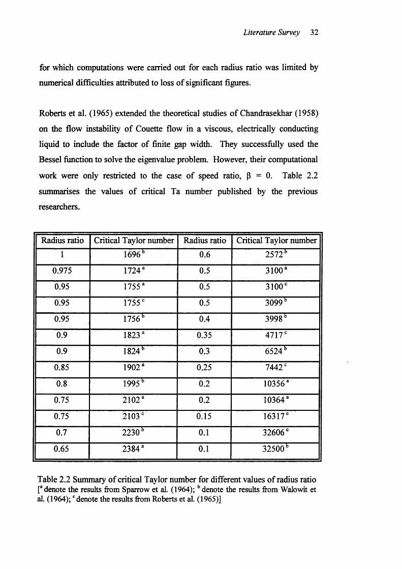
Literature Survey 32
for which computations were carried out for each radius ratio was limited by
numerical difficulties attributed to loss o f significant figures.
Roberts et al. (1965) extended the theoretical studies of Chandrasekhar (1958)
on the flow instability o f Couette flow in a viscous, electrically conducting
liquid to include the factor of finite gap width. They successfully used the
Bessel function to solve the eigenvalue problem. However, their computational
work were only restricted to the case of speed ratio, p = 0. Table 2.2
summarises the values o f critical Ta number published by the previous
researchers.
Radius ratio Critical Taylor number Radius ratio Critical Taylor number
1 1696" 0.6 2572"
0.975 1724* 0.5 3100*
0.95 1755* 0.5 3100"
0.95 1755" 0.5 3099"
0.95 1756" 0.4 3998"
0.9 1823* 0.35 4717"
0.9 1824" 0.3 6524"
0.85 1902* 0.25 7442"
0.8 1995" 0.2 10356*
0.75 2102* 0.2 10364*
0.75 2103" 0.15 16317"
0.7 2230" 0.1 32606"
0.65 2384* 0.1 32500"
Table 2.2 Summary of critical Taylor number for different values o f radius ratio P denote the results from Sparrow et al. (1964); denote the results from Walowit et a i. (1964); ‘'denote the results from Roberts et al. (1965)]
Literature Survey 33
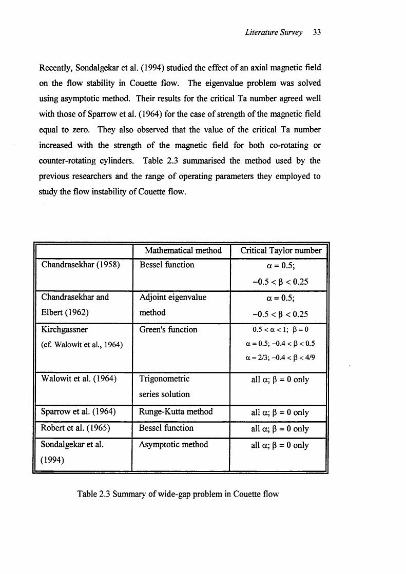
Recently, Sondalgekar et al. (1994) studied the effect of an axial magnetic field
on the flow stability in Couette flow. The eigenvalue problem was solved
using asymptotic method. Their results for the critical Ta number agreed well
with those o f Sparrow et al. (1964) for the case o f strength of the magnetic field
equal to zero. They also observed that the value of the critical Ta number
increased with the strength of the magnetic field for both co-rotating or
counter-rotating cylinders. Table 2.3 summarised the method used by the
previous researchers and the range o f operating parameters they employed to
study the flow instability o f Couette flow.
Mathematical method Critical Taylor number
Chandrasekhar (1958) Bessel function a = 0.5;
-0.5 < P < 0.25
Chandrasekhar and
Elbert (1962)
Adjoint eigenvalue
method
a = 0.5;
-0.5 < P < 0.25
Kirchgassner
(of. Walowit et al., 1964)
Green's function 0.5 < a < 1; p = 0
a = 0.5; -0.4 < p < 0.5
a = 2/3; -0.4 < P < 4/9
Walowit et al. (1964) Trigonometric
series solution
all a; P = 0 only
Sparrow et al. (1964) Runge-Kutta method all a; P = 0 only
Robert et al. (1965) Bessel function all a; P = 0 only
Sondalgekar et al.
(1994)
Asymptotic method all a; P = 0 only
Table 2.3 Summary of wide-gap problem in Couette flow
Literature Survey 34
2.2.3 Narrow-aap problem in Couette flow with a low axial flow
When a low axial flow is superimposed on the Couette flow, the problem
becomes more complicated. This combined flow, so-called Couette-Poiseuille
flow, occurs in numerous industrial applications. A number of investigations
have been conducted to establish the effect o f axial flow on the occurrence of
Taylor vortices in a laminar flow. The critical Ta number was found to be a
function o f the axial Reynolds number. Re, the radius ratio, a, and the angular
speed ratio, p, o f the concentric rotating cylinders.
Goldstein (1937) first considered this problem theoretically for the case o f the
outer cylinder at rest and the small-gap width compared to the mean radius. He
used the method of expansion in Fourier series and treated the case o f flow
between rotating cylinders in the presence of an axial pressure gradient along
the axis o f the cylinders. Goldstein (1937) showed that the critical Ta number
initially increased, as the Re number (associated with the axial flow velocity),
increased from zero to a value of about 20, and then decreased rapidly as Re
increased to 25.
Chandrasekhar (1961) showed that Rayleigh's inviscid criterion for rotational
instability, as previously applied to viscous and purely rotational flow between
concentric rotating cylinders, remained valid in the presence o f an axial
velocity components. To account for viscosity effects Chandrasekhar (1961)
and simultaneously Di Prima (1960) employed linear theory to predict critical
Ta number in narrow-gap for the case of cylinders in co-rotating fully
developed laminar Couette flow for Re number below 200. Chandrasekhar
(1960) considered the tangential velocity to be uniform across the gap, an
assumption justified by extrapolation from the findings of Taylor (1923) for
zero Re number, where a small error in the predicted critical Ta number was
reported. His predictions of critical Ta number compared well with those o f Di
Literature Survey 35
Prima (1960) using the same assumptions but the latter also found the
substitution of a parabolic axial velocity distribution to have an effect o f no
more than 5.5% on the solution for Re < 80, compared with uniform axial
velocity case. At higher Re number the values of critical Ta number for the
two cases diverged. For a stationary outer cylinder, critical Ta number
increased approximately with Re " and Re ^ for a parabolic and a uniform
velocity respectively; the corresponding value of critical Ta number at Re =
120 were 15126 and 11850 respectively.
Chandrasekhar (1962) considered the case when the axial velocity profile was
parabolic and developed a perturbation theory which was valid in the very low
range of values of Re number. He found that the critical Ta number increased
more rapidly than predicted by Di Prima's (1960) solutions. Chandrasekhar
(1962) used a perturbation procedure, and found that
Tac = Tac(atRe = o) + 26.5 Re a sR e -> 0 [2.5]
Later Krueger and Di Prima (1964) re-examined the same problem, and
obtained their results by using Fourier series technique. The predictions agreed
with the earlier results of Di Prima (1960) but did not show the rapid initial
increase o f the critical Ta number with Re number as reported by
Chandrasekhar (1962). Their results were an improvement on Di Prima's
(1960) previous work. They also suggested that, while the perturbation
procedure used by Chandrasekhar (1962) was suitable, in the actual
computation not enough terms in the series had been retained to give the correct
coefficients o f Re^ in Eq. [2.5].
Hughes and Reid (1968) treated the case o f large Re number (> 200) in a
narrow-gap situation using a uniform tangential distribution. They used an
asymptotic method whereby the resultant equations could be approximated by
the Orr-Sommerfield equation; their prediction for a parabolic axial distribution
Literature Survey 36
appeared consistent with those of Di Prima (1960). All the above theoretical
evidence indicates that the use o f an average axial velocity leads to
underprediction of the critical Ta number by a factor which increases with Re
number for values o f Re number above 80.
Elliott (1973) used the same approach as that o f Krueger and Di Prima (1964),
but with more terms in the algebraic series formulation. His calculations for Re
number up to 200 with a parabolic axial velocity distribution and a linear
approximation to the exact fully developed tangential velocity profile, agreed
with Di Prima's prediction. Table 2.4 summarised the method used by the
previous researchers and the range o f operating parameters they employed to
study the flow instability of Couette flow with axial flow.
Mathematical method Critical Taylor number
Goldstein (1937) Fourier series expansion 0 < Re < 50
p = oChandrasekhar (1961) Bessel function R e -» 0
p = oDi Prima (1960) Algebraic series Re < 200
p = oChandrasekhar ( 1962) Expansion of
Bessel function
R e ^ O
Krueger and Di Prima
(1964)
Fourier series expansion 0 < Re < 40
allp
Hughes and Reid
(1968)
Asymptotic method Re > 200
Elliott (1973) Algebraic series 0 < R e < 100
Table 2.4 Summary of narrow-gap problem in Couette flow with axial flow
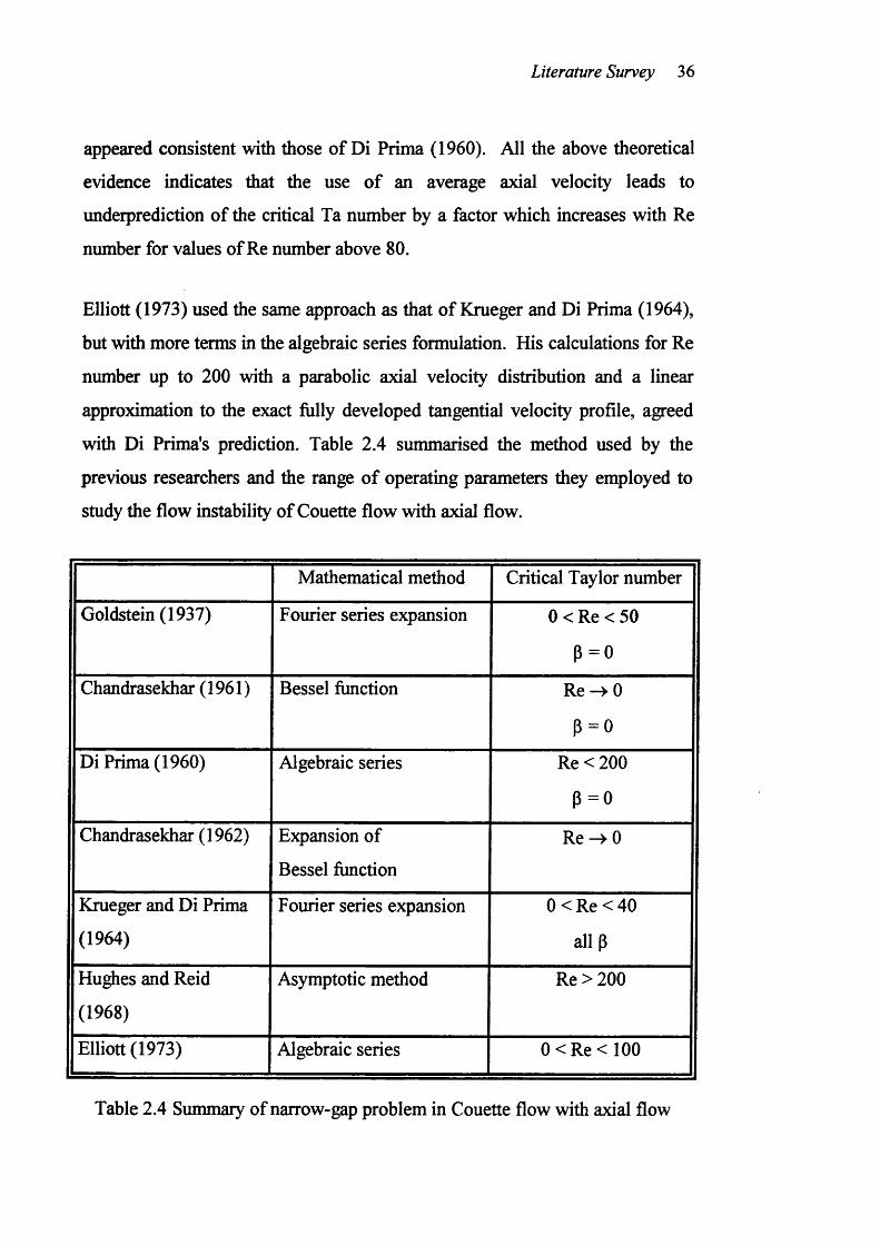
Literature Survey 37
2.2.4 Wide-gap problem in Couette flow with a low axial flow
So far we have dealt with the narrow-gap case in Couette-Poiseuille flow only.
The corresponding wide-gap stability problem has received rather less attention
because o f its complex nature and very tedious computations involved. One of
the difficulties in treating the wide-gap problem is that the differential operators
in the eigenvalue problem have variable coefficients in contrast to the constant
coefficient operators that appear in the small gap problem.
Hasoon and Martin (1977) predicted the critical Ta number and critical wave
numbers for axial symmetrical flow. Using both a time-dependent finite-
difference procedure and solution employing the Galerkin method, they
computed results for radius ratios between 0.81 and 0.95 and for Re number up
to 1000. They questioned the use of a parabolic form for the axial velocity
profile in the stability problem. However, their predictions were restricted to
the angular speed ratio equal to zero.
Chung and Astill (1977) treatment were based on linear stability theory plus a
shooting method for the fully developed axial and tangential velocity
distributions; their theory covered initially axisymmetric disturbances only for
radius ratio, a = 0.95 and initially non-axisymmetric disturbances over the
range 0.1 < a < 0.95, Re number up to 300 and cases with co-rotating and
counter-rotation of the cylinders. In this general case, the stability analysis
required two wave numbers: the axial wave number and azimuthal wave
number. The linear stability limit is then found by determining the minimum
on the family of neutral stability curves. In this regard, the minimisation
process used by Chung and Astill (1977) was too difficult to follow. Moreover,
there was no theoretical justification for this assumption so that the treatment of
the problem with a general disturbance must be regarded as incomplete. Some
Literature Survey 38
additional comments on the minimisation process used by Chung and Astill
(1977) were provided by Di Prima and Pridor (1979).
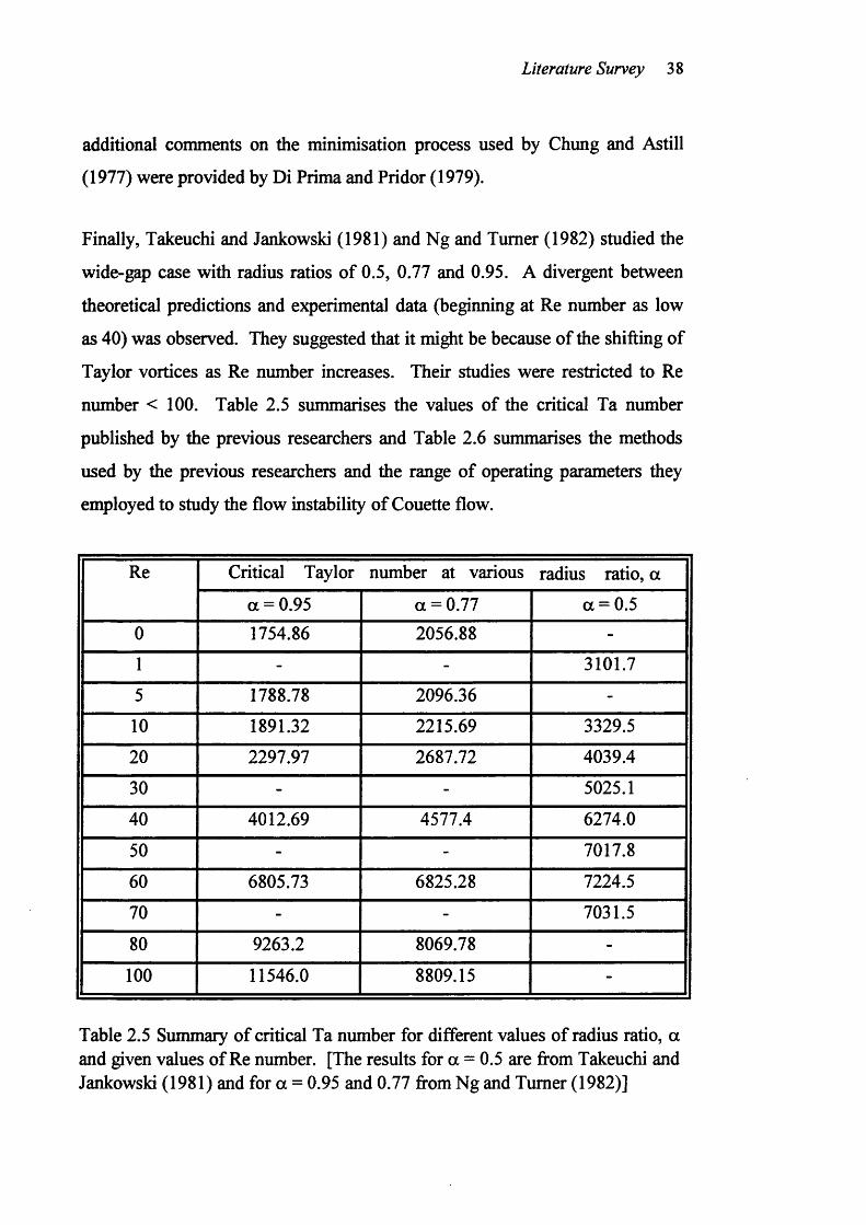
Finally, Takeuchi and Jankowski (1981) and Ng and Turner (1982) studied the
wide-gap case with radius ratios o f 0.5, 0.77 and 0.95. A divergent between
theoretical predictions and experimental data (beginning at Re number as low
as 40) was observed. They suggested that it m i^ t be because of the shifting of
Taylor vortices as Re number increases. Their studies were restricted to Re
number < 100. Table 2.5 summarises the values of the critical Ta number
published by the previous researchers and Table 2.6 summarises the methods
used by the previous researchers and the range o f operating parameters they
employed to study the flow instability of Couette flow.
Re Critical Taylor number at various radius ratio, a
a = 0.95 a = 0.77 a = 0.5
0 1754.86 2056.88 -
1 - - 3101.7
5 1788.78 2096.36 -
10 1891.32 2215.69 3329.5
20 2297.97 2687.72 4039.4
30 - - 5025.1
40 4012.69 4577.4 6274.0
50 - - 7017.8
60 6805.73 6825.28 7224.5
70 - - 7031.5
80 9263.2 8069.78 -
100 11546.0 8809.15 -
Table 2.5 Summary of critical Ta number for different values of radius ratio, a and given values o f Re number. [The results for a - 0.5 are from Takeuchi and Jankowski (1981) and for a = 0.95 and 0.77 from Ng and Turner (1982)]
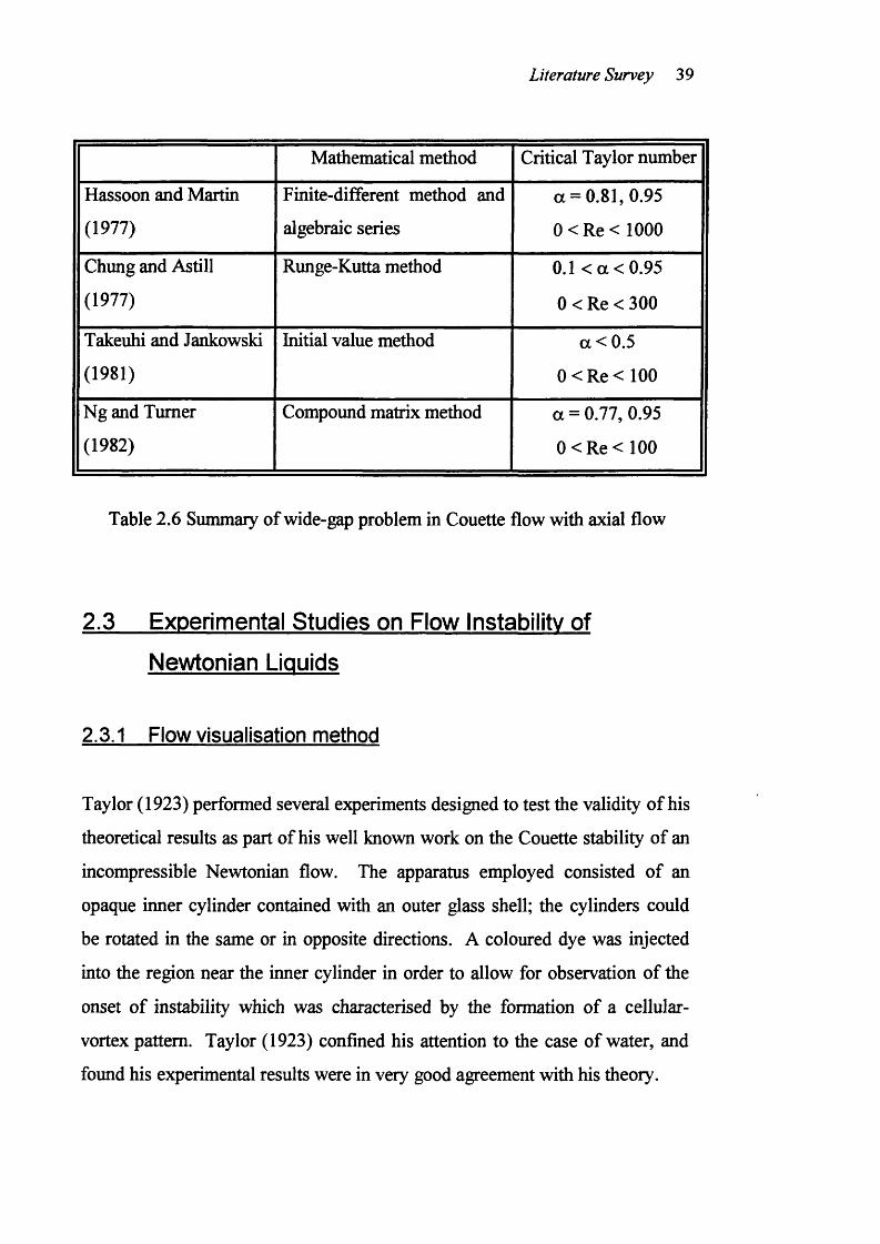
Literature Survey 39
Mathematical method Critical Taylor number
Hassoon and Martin
(1977)
Finite-different method and
algebraic series
a = 0.81, 0.95
0 < R e < 1000
Chung and Astill
(1977)
Runge-Kutta method 0.1 < a < 0.95
0 < Re < 300
Takeuhi and Jankowski
(1981)
Initial value method a < 0.5
0 < R e < 100
Ng and Turner
(1982)
Compound matrix method a = 0.77, 0.95
0 < R e < 100
Table 2.6 Summary of wide-gap problem in Couette flow with axial flow
2.3 Experimental Studies on Flow Instability of
Newtonian Liquids
2.3.1 Flow visualisation method
Taylor (1923) performed several experiments designed to test the validity of his
theoretical results as part of his well known work on the Couette stability of an
incompressible Newtonian flow. The apparatus employed consisted of an
opaque inner cylinder contained with an outer glass shell; the cylinders could
be rotated in the same or in opposite directions. A coloured dye was injected
into the region near the inner cylinder in order to allow for observation of the
onset o f instability which was characterised by the formation of a cellular-
vortex pattern. Taylor (1923) confined his attention to the case of water, and
found his experimental results were in very good agreement with his theory.
Literature Survey 40
Lewis (1928) extended Taylor's findings to cover a wide range o f Newtonian
liquids. The liquid motion in his study was followed by means of tiny
suspended aluminum particles rather than by dye injection. Thus, the problem
of diffusion of dye into the liquid was avoided, and each experiment could be
repeated several times for the same sample.
Coles (1965) later showed the complex flow regimes occurring beyond the
Taylor-Couette flow regime. In his study of flow between both counter and co-
rotating cylinders Coles (1965) discovered several very distinctive flow
regimes, including double periodic flow, intermittent turbulent bursts and spiral
turbulence as the rotational speed further increased. He also stated that at a
given Ta number there were several distinct stable flow states, depending upon
the Ta number history, i.e., how to reach the final Ta number.
Koschmieder (1979) later found that the wavelength increased with increasing
Ta number only up to Ta/Tac - 1 0 . He also studied turbulent vortex flow
between long concentric cylinders and measured the axial wavelength o f Taylor
vortices by suspending aluminum powder in the liquid. He found that the
wavelength became substantially larger than the critical wavelength of laminar
Taylor vortices.
Andereck et al. (1983 and 1986) reported many reproducible flow states
obtained by systematic variation of inner and outer cylinder speed. They also
observed five new flows regimes occurring in the case o f co-rotating cylinders.
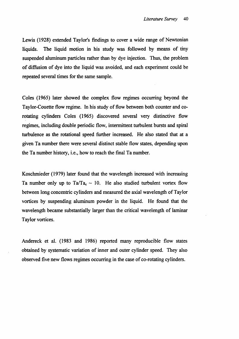
Fluid medium Materials added for visualisation Radius ratio Ta number studied
Taylor (1923) Water Eosin (dye) 0.942 0 <Ta/Iac < 1
Lewis (1928) Xylene,
Nitrobenzene
Suspended particle 0.829 0 <Ta/Tac < 4
Coles (1965) Silicon oil Aluminum powder 0.888 0 < Ta/Tac <100
Koschmieder (1979) Water Aluminum powder 0.896 0 < Ta/Tac <40,000
Andereck et al. (1983 and 1986) Water Polymeric flakes 0.883 0< T a /Iac< 19
Gu and Fahidy
(1985a, b)
Electrolyte
solution (acidic)
Analytical indicators 0.714 0 < Ta/Tac <23
Benjamin (1987a, b) Glycerol Pearl substance 0.615 0.3 < Ta/Tac <3.2
Table 2.7 Suiranaiy o f major experiments on flow visualisation method in Couette flow device
Literature Survey 42
Gu and Fahidy (1985a, b) investigated the changes in the structure of the
vortices with increasing axial velocity by using a visualisation technique. At
small axial flows the individual Taylor cells were inclined and partial
overlapping of cells occurred. With further increase in the axial flow rate, the
cell structure degenerated progressively to a disorderly pattern. At high axial
flow rates the Taylor cells were hardly detectable and the complete
degeneration of Taylor vortices was assumed.
Finally, Benjamin (1987a, b) observed different states in Taylor vortex flow
even in an annulus so short that only 3 to 4 vortices could be accommodated.
Table 2.7 summarised the major experiments on flow visualisation in Couette
flow device.
2.3.2 Flow spectra method
Fenstermacher et al. (1979) first used the velocity power spectra method to
study the transition to turbulence for flow between concentric cylinders. The
liquid velocity was determined from measurements o f the Doppler shift of
scattered laser light. The Doppler shifts were typically ~ 10 Hz while the
characteristic frequencies o f the liquid were -0 .1 to 10 Hz, so measurements of
the Doppler shift in short time intervals yielded essentially the instantaneous
liquid velocity. They showed that different dynamic flow regimes could be
distinguished by examining high-resolution power spectra of a time-dependent
property of the flow. Transitions that were obvious in the power spectra, such
as the broadening of a spectral line or the appearance of a new characteristic
frequency in the flow, could be undetected in a direct inspection of the time
records or flow photographs. Thus power spectra method have become a major
tool for the study of the transition from laminar to turbulent flow.
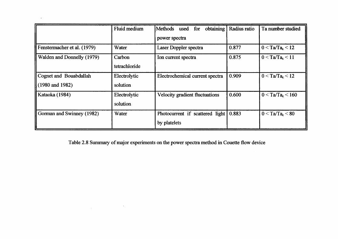
Fluid medium Methods used for obtaining
power spectra
Radius ratio Ta number studied
Fenstermacher et al. (1979) Water Laser Doppler spectra 0.877 0 < Ta/Tac < 12
Walden and Donnelly (1979) Carbon
tetrachloride
Ion current spectra 0.875 0 < T a /T a c< ll
Cognet and Bouabdallah
(1980 and 1982)
Electrolytic
solution
Electrochemical current spectra 0.909 0 < Ta/Tac < 12
Kataoka (1984) Electrolytic
solution
Velocity gradient fluctuations 0.600 0 < Ta/Tac <160
Gorman and Swinney (1982) Water Photocurrent if scattered light
by platelets
0.883 0 <T a/ Tac <8 0
Table 2.8 Summary o f major experiments on the power spectra method in Couette flow device
Literature Survey 44
Walden and Donnelly (1979) simultaneously studied the transitions in the flow
between concentric cylinders by an entirely different measurement technique.
They measured the ion current between a collector embedded in the outer
cylinder wall and the gold-plated inner cylinder as a function of time. The
records were Fourier-transformed to obtain ion current power spectra, in which
the results were in agreement with Fenstermacher et al. (1979).
Cognet and his coworker (1980 and 1982) measured the radial gradient of the
azimuthal velocity on the outer cylinder wall by using an electrochemical
technique and analysed the velocity-gradient spectra by means of an electronic
spectrum analyser. They found that turbulence regime originated from the
vortex outflow boundaries.
Kataoka et al. (1984) applied similar diffusion-controlled electrolytic reaction
and analysed the power spectra of the velocity-gradient fluctuations on the
outer cylinder wall for explanation o f the dynamical modes of ionic mass
transfer measured on the outer cylinder wall.
Gorman and Swinney (1982) measured the power spectra of the intensity of
light scattered by the fine platelets that aligned with the flow. They discovered
many distinct wave patterns in the doubly periodic flow. Table 2.8 gives a
summary o f the major experiments on power spectra method in Couette flow
device.
2.3.3 Dispersion measurement
Kataoka et al. (1975) first experimentally studied the mixing property of the
axially moving Taylor vortex flow in connection with the application of this
flow system to chemical equipment. They made measurements of the
intermixing over cell boundary between Taylor vortices for very small axial
Literature Survey 45
flow rates by measuring the residence time distribution using two probes placed
on the inner surface o f the outer cylinder. All o f their measurements were
taken in the range of 1 < Ta/Tac <12. And 0 < Re < 23. They showed that the
toroidal vortices motion o f liquid elements caused highly effective radial
mixing within cellular vortices, whereas the cell boundaries prevented liquid
elements from being exchanged over the vortex inflow boundaries. Each pair
of vortices could be regarded as a well-mixed batch vessel, which moved
axially at a constant velocity. The vortices, whose size was approximately
equal to the annular gap, marched through the annulus at a constant velocity
equal to the mean axial velocity. Therefore, it could be considered that all the
liquid elements leaving the annulus had the same residence time in the
apparatus.
Kataoka et al. (1975) showed that Taylor-Couette flow was one of the rare flow
types combining ideal plug flow with ideal stirred tank behaviour. This
publication has become the key reference in the field of Taylor-Couette flow
mixing. Their assumption of non-intermixing vortices however was based upon
qualitative interpretations o f tracer experiments. Nevertheless, it has been
adopted in all subsequent published calculations of reactor productivity in the
laminar regime (Cohen and Maron, 1983).
Kataoka et al. (1977) later attempted to quantitatively investigate the extent to
which Taylor-Couette flow offers this unusual combination of mixing
properties. They made local measurements of mass transfer on the inner wall
of outer stationary cylinder by means of an electrochemical technique. The test
section was far down stream from entry, so that Taylor vortex structure could
be established in laminar axial flow. For a small forced axial flow (0 < Re <
130), toroidal vortices marched through in single file without breaking up. As
the Re number increased gradually, the regular variation of Sherwood number
(associated with the rate of mass exchange) was not only distorted by the
Literature Survey 46
forced axial motion, but also its mean value was reduced greatly. Kataoka et
al. (1977) also showed that during the Taylor-Couette flow regime, the added
axial motion tended to stabilise the circular Couette flow and to delay the initial
formation of Taylor vortices.
Kataoka et al. (1981) identified the existence of a small mass flux between
adjacent vortices for 1 < Ta/Tac < 12 and 0 < Re < 18. They measured the rate
of exchange of liquid elements between the boundaries of vortices by using the
same method as Kataoka et al. (1975). They assumed that each vortex unit
behaved as an ideal stirred tank and quantified the inter-vortex flux with a
localised inter-vortex mass transfer coefficient. They stated that the rate of
circumferential and radial mixing was much faster compared to axial mixing.
Legrand and Coeuret (1986) and Guihard et al. (1989) published the residence
time distribution measurements, for a range of Ta number, from which they
claimed the total absence of vortex-intermixing, thereby confirming the first
conclusion of Kataoka et al. (1975). They assumed that the tracer material
would be bounded by the vortices' boundaries as the radius ratio was smaller
than 0.72. This assumption was also supported by Coles (1965) and Gu and
Fahidy (1986). So that, the circumferential dispersion coefficient De, was
calculated based on the equation of tank-in-series model. They showed the
value was negligibly small that the tracer material would be entirely consumed
in a vortex cell behaved like a closed reactor.
Recently, Pudjiono et al. (1992) restricted their experiments to the laminar flow
regime (very slow or zero rotational flow where Taylor vortices were absent)
and the Taylor-Couette flow regime. All of their measurements were carried in
the range of 0 < Ta/Tac < 2 and 0.4 < Re < 5.5. The residence time distribution
(RTD) measurements were restricted to the outer layers and the dispersion
coefficient was determined from the variance of RTD curves recorded.
Literature Survey 47
Pudjiono et al. (1992) observed that the flow became fairly unstable below the
critical Ta number. When Ta number reached the critical value, Ta , a peak in
the shape of the RTD function was observed due to good radial mixing induced
by the Taylor vortex flow. In their study a minimum dispersion coefficient was
used to characterize the critical Ta number. The results were in agreement with
previous researchers by implying that 'near' plug-flow could be obtained as the
critical Ta number was reached.
Pudjiono and Tavare (1993) further obtained RTD data around the critical Ta
number in the ranges 0 < Ta < 2.5 and 0 < Re < 5.5. They found that
dispersion coefficient increased fi*om a minimum value as the Ta number
increased beyond its critical value. It was suggested that the 'near' plug flow
behaviour occurred only at critical Ta number.
Croockewit et al. (1955) studied the axial dispersion coefficient o f a Newtonian
liquid in a continuous Couette flow device based on the fi*equency response
analysis o f RTD. All o f their measurements were taken at rotational speeds
much higher than the critical Ta number. The sinusoidal frequency and phase
shift o f the electrical conductivity changes of the liquid following the injection
were recorded by using two small conductivity probes placed inside the
Couette flow-device. By comparing the records from both probes under a
given set of conditions, the values o f axial dispersion coefficient were
calculated based on the equations of dispersion model.
Croockewit et al. (1955) showed that the calculated values of dispersion
coefficient were in the range 0.3 x IC to 3.0 x 10^ m s" in their experiments
and these were independent of Re number when the axial flow velocity are low
compared to the tangential velocity of the liquid.
Literature Survey 48
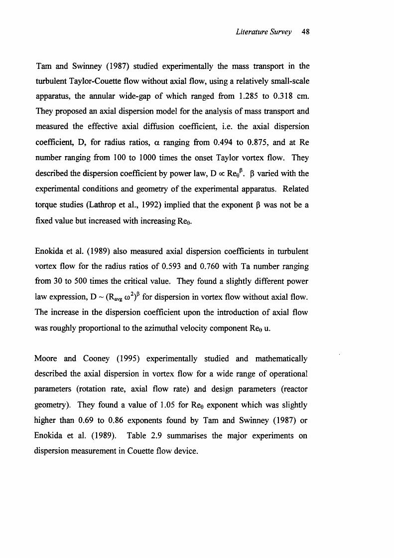
Tam and Swinney (1987) studied experimentally the mass transport in the
turbulent Taylor-Couette flow without axial flow, using a relatively small-scale
apparatus, the annular wide-gap of which ranged from 1.285 to 0.318 cm.
They proposed an axial dispersion model for the analysis o f mass transport and
measured the effective axial diffusion coefficient, i.e. the axial dispersion
coefficient, D, for radius ratios, a ranging from 0.494 to 0.875, and at Re
number ranging from 100 to 1000 times the onset Taylor vortex flow. They
described the dispersion coefficient by power law, D oc Ree . P varied with the
experimental conditions and geometry of the experimental apparatus. Related
torque studies (Lathrop et al., 1992) implied that the exponent p was not be a
fixed value but increased with increasing Ree.
Enokida et al. (1989) also measured axial dispersion coefficients in turbulent
vortex flow for the radius ratios of 0.593 and 0.760 with Ta number ranging
from 30 to 500 times the critical value. They found a slightly different power
law expression, D ~ (Ravg co ) for dispersion in vortex flow without axial flow.
The increase in the dispersion coefficient upon the introduction of axial flow
was roughly proportional to the azimuthal velocity component Ree u.
Moore and Cooney (1995) experimentally studied and mathematically
described the axial dispersion in vortex flow for a wide range of operational
parameters (rotation rate, axial flow rate) and design parameters (reactor
geometry). They found a value of 1.05 for Ree exponent which was slightly
higher than 0.69 to 0.86 exponents found by Tam and Swinney (1987) or
Enokida et al. (1989). Table 2.9 summarises the major experiments on
dispersion measurement in Couette flow device.
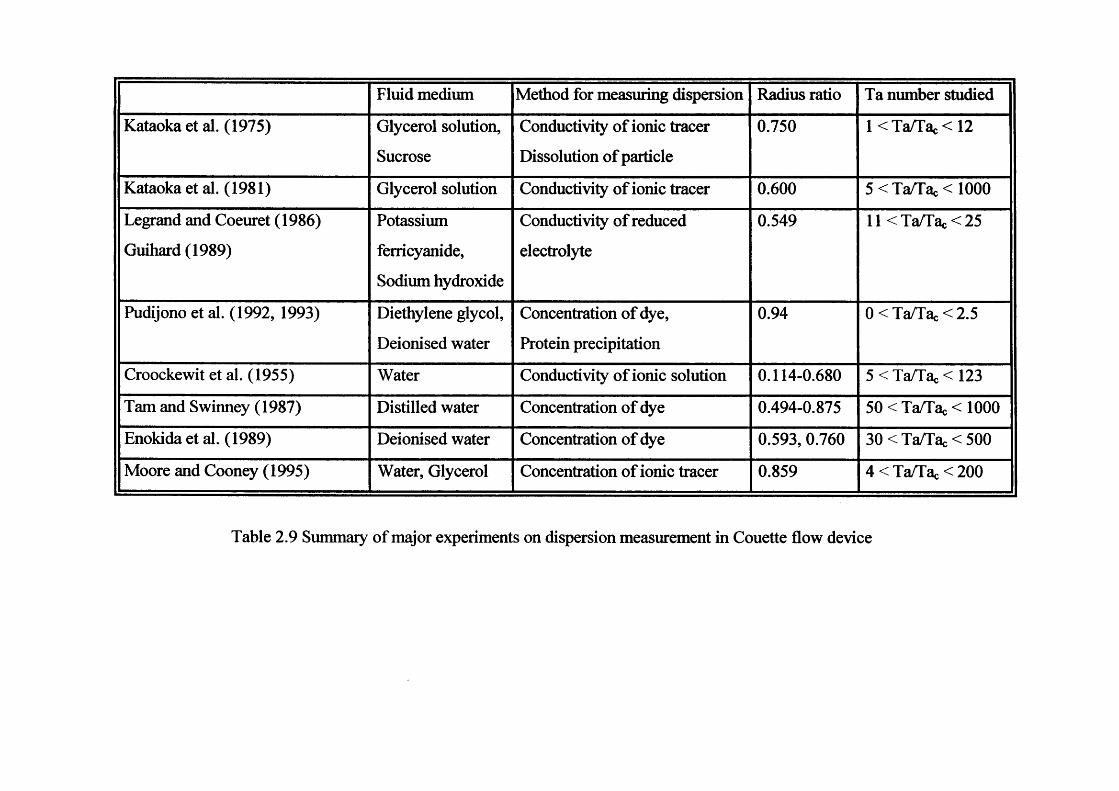
Fluid medium Method for measuring dispersion Radius ratio Ta number studied
Kataoka et al. (1975) Glycerol solution.
Sucrose
Conductivity o f ionic tracer
Dissolution of particle
0.750 1 < Ta/Tac < 12
Kataoka et al. (1981) Glycerol solution Conductivity o f ionic tracer 0.600 5 < Ta/Tac < 1000
Legrand and Coeuret (1986)
Guihard (1989)
Potassium
ferricyanide.
Sodium hydroxide
Conductivity of reduced
electrolyte
0.549 ll< T a/T ac< 25
Pudijono et al. (1992, 1993) Diethylene glycol.
Deionised water
Concentration o f dye.
Protein precipitation
0.94 0 < Ta/Tac <2.5
Croockewit et al. (1955) Water Conductivity o f ionic solution 0.114-0.680 5 < Ta/Tac < 123
Tam and Swinney (1987) Distilled water Concentration o f dye 0.494-0.875 50 < Ta/Tac < 1000
Enokida et al. (1989) Deionised water Concentration o f dye 0.593, 0.760 30 < Ta/Tac <500
Moore and Cooney (1995) Water, Glycerol Concentration o f ionic tracer 0.859 4 < Ta/Tac <200
Table 2.9 Summary o f major experiments on dispersion measurement in Couette flow device
Literature Survey 50
2.4 Theoretical Studies on Flow Instability of
Non-Newtonian Liquids
Graebel (1961) studied the Couette stability of non-Newtonian liquids. By
employing the small-gap approximation to simplify the analysis, Graebel found
that the viscosity can strongly influence the results obtained for the critical
Taylor number. Although Graebel's analysis has been performed for the
somewhat unrealistic conditions, it did give some general indication o f what
one might expect for non-Newtonian liquids and showed that the critical Taylor
number depended on the non-Newtonian properties o f the liquid.
Ginn and Denn (1969) and Sun and Denn (1972) considered the general case of
stability of liquids exhibiting weak elastic properties and used the narrow-gap
approximation. Both groups showed the results obtained for one set of
rheological parameter. Their results were in good agreement with the
experimental data carried out for polymer solutions exhibiting shear thinning
behaviour. They also found that the critical Ta number increased or decreased
depending on the value of two dimensionless groups associated with the normal
stress coefficients.
Larson (1990) carried out a linear stability analysis for the case of the narrow-
gap, using the Doi-Edwards model which accounts qualitatively for both
normal stress and shear thinning effects. He recognised that the combination of
elastic and pseudoplastic effects was important for concentrated polymer
solution. The results showed that the shear thinning behaviour described by the
Doi-Edwards equation has a destabilising influence on the flow. Larson (1990)
also obtained a numerical solution for the Taylor-Couette flow for an upper-
convected Maxwell liquid neglecting the inertia.
Literature Survey 51
2.5 Experimental Studies on Flow Instability of
Non-Newtonian Liquids
Giesekus (1972), using polyacrylamide solution, showed that the critical value
of the Ta number at the onset o f Taylor vortices could be smaller or larger than
the Newtonian value depending on polymer concentration. At high polymer
concentration, when elastic effects become dominate, the critical Re number
was found to decrease with the flow Weissenberg number (given as the product
of the liquid's longest relaxation time and the shear rate). However, at high
polymer concentration, solution might exhibit significant shear thinning.
Giesekus's (1972) experiments were generally in agreement with his own
theoretical studies for dilute polymer solution, but showed an unexplained
decrease in the critical Ta number of up to 50% as the polymer concentration
approached 1000 ppm. He stated that both viscoelastic and shear thinning
effects must be accounted for through a suitable constitutive model.
Sinevic et al. (1985) experimentally investigated the Couette flow instability by
means o f a power number as a function of Ta numbers. All the experiments
were performed with carboxymethyl cellulose solutions for radius ratio greater
than 0.6. Sinevic et al. (1985) also defined the Ta number on the basis of the
apparent viscosity value at the inner rotating cylinder. Experimental results
showed that the critical Ta number was dependent on the gap width and on the
flow index, n. In most cases, the critical Ta number was found to be larger
than a Newtonian liquid with similar viscosity but it approached the Newtonian
value asymptotically as the value of the critical Ta number decreased with the
decrease of pseudoplasticity. Tables 2.10 and 2.11 summarise the theoretical
and experimental studies o f non-Newtonian liquids in Couette flow device.
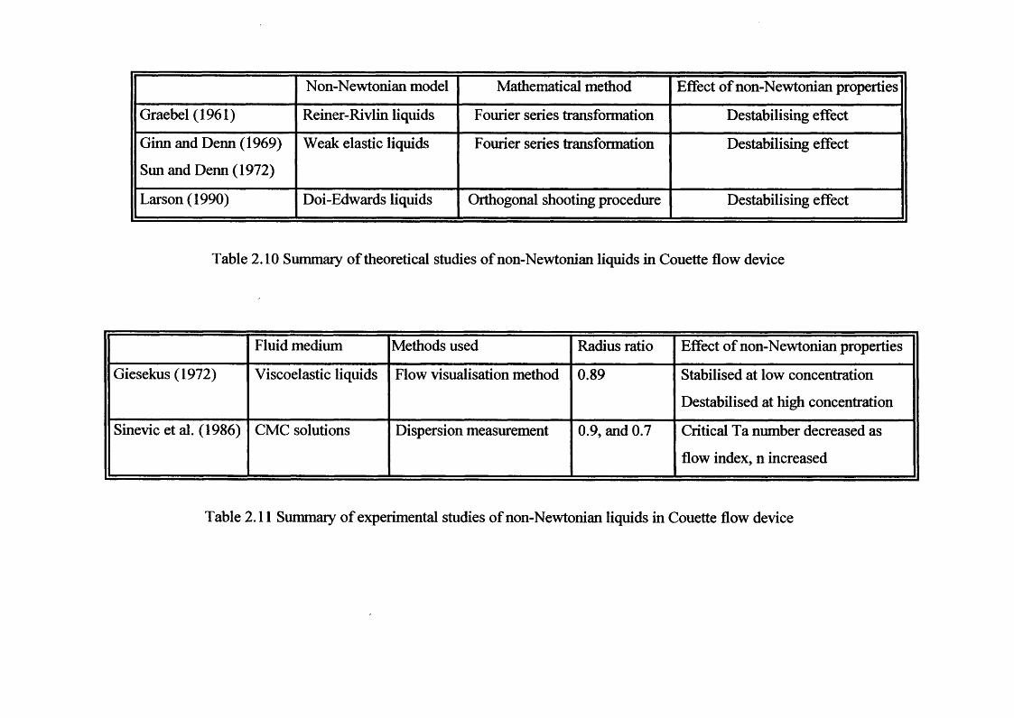
Non-Newtonian model Mathematical method Effect o f non-Newtonian properties
Graebel (1961) Reiner-Rivlin liquids Fourier series transformation Destabilising effect
Ginn and Denn (1969)
Sun and Denn (1972)
Weak elastic liquids Fourier series transformation Destabilising effect
Larson (1990) Doi-Edwards liquids Orthogonal shooting procedure Destabilising effect
Table 2.10 Summary o f theoretical studies o f non-Newtonian liquids in Couette flow device
Fluid medium Methods used Radius ratio Effect o f non-Newtonian properties
Giesekus (1972) Viscoelastic liquids Flow visualisation method 0.89 Stabilised at low concentration
Destabilised at high concentration
Sinevic et al. (1986) CMC solutions Dispersion measurement 0.9, and 0.7 Critical Ta number decreased as
flow index, n increased
Table 2.11 Summary o f experimental studies o f non-Newtonian liquids in Couette flow device
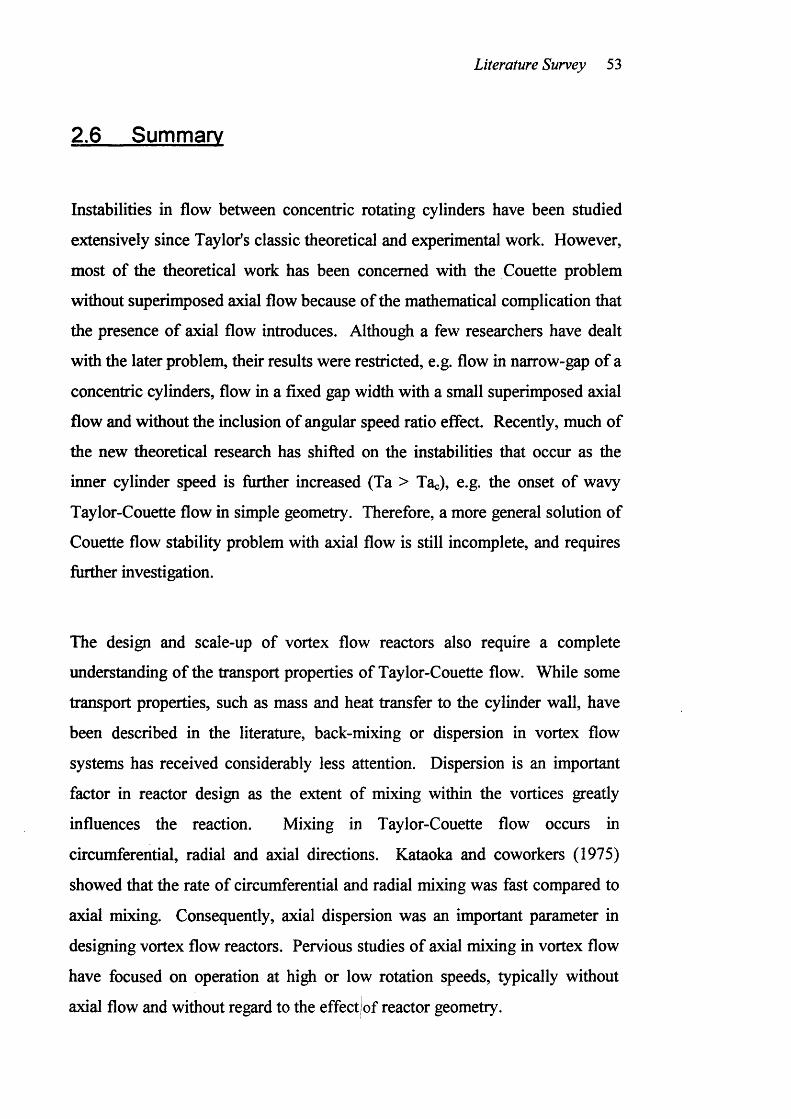
Literature Survey 53
2.6 Summary
Instabilities in flow between concentric rotating cylinders have been studied
extensively since Taylor's classic theoretical and experimental work. However,
most of the theoretical work has been concerned with the Couette problem
without superimposed axial flow because of the mathematical complication that
the presence of axial flow introduces. Although a few researchers have dealt
with the later problem, their results were restricted, e.g. flow in narrow-gap of a
concentric cylinders, flow in a fixed gap width with a small superimposed axial
flow and without the inclusion o f angular speed ratio effect. Recently, much of
the new theoretical research has shifted on the instabilities that occur as the
inner cylinder speed is further increased (Ta > Tac), e.g. the onset o f wavy
Taylor-Couette flow in simple geometry. Therefore, a more general solution of
Couette flow stability problem with axial flow is still incomplete, and requires
further investigation.
The design and scale-up of vortex flow reactors also require a complete
understanding of the transport properties o f Taylor-Couette flow. While some
transport properties, such as mass and heat transfer to the cylinder wall, have
been described in the literature, back-mixing or dispersion in vortex flow
systems has received considerably less attention. Dispersion is an important
factor in reactor design as the extent o f mixing within the vortices greatly
influences the reaction. Mixing in Taylor-Couette flow occurs in
circumferential, radial and axial directions. Kataoka and coworkers (1975)
showed that the rate o f circumferential and radial mixing was fast compared to
axial mixing. Consequently, axial dispersion was an important parameter in
designing vortex flow reactors. Pervious studies o f axial mixing in vortex flow
have focused on operation at high or low rotation speeds, typically without
axial flow and without regard to the effect|of reactor geometry.
Literature Survey 54
Relatively little work has been devoted to the case of non-Newtonian liquids.
One of main reasons is the variation of the apparent viscosity o f liquids in the
cross-section o f the annular gap. The dependence of the predicted flow
behaviour on the choice o f a constitutive model is another difficulty in
attempting to interpret an already complex flow situation. Moreover, the non-
Newtonian constitutive equations often involve rheological parameters such as
flow index and consistency index. Recently, computer-assisted linear stability
analyses have been extended to non-Newtonian liquids, even involving an
analysis o f the possible pattern of the Taylor vortices established after the onset
o f the instability. However, most o f the researches to date have been restricted
to the small-gap geometry for mathematical simplicity. Except for narrow-gap
geometry, one rarely finds the complete solution because o f the complicated
link between stress and strain of the non-Newtonian liquids. It is therefore the
aim of the present investigation to show how this analysis can be extended to
arbitrary gaps, and to discuss the influence of the rheological parameters on the
basic velocity field as well as on the onset of the Taylor-Couette flow.
There are a few experimental investigations of the properties of polymer
solution (i.e. viscoelastic liquids) on the Taylor-Couette instability problem. In
general, these workers have found that viscoelasticity increases the critical Ta
number at which a cellular flow is observed. Thus, the addition of
viscoelasticity stabilises the flow against the formation of Taylor vortices.
None o f the research works cited so far investigated the effect o f Taylor vortex
flow on mass transport (residence time distribution) on non-Newtonian
pseudoplastic liquids. Investigation on the mass transfer characteristic o f non-
Newtonian liquids can lead to an understanding of the fundamental aspects of
this process.
Theory 55
CHAPTER THREE
THEORY
3.1 Introduction
In Section 3.2, the theoretical consideration is extended to a more general
Couette flow problem between concentric rotating cylinders when, in addition
to rotation, a constant axial flow velocity is present. Previous work has shown
that in Couette flow, the streamlines continue to be circular. However, when a
Poiseuille flow is superimposed over the same distribution of rotational
velocities, the streamlines are no longer circular and the flow cannot be treated
as Couette flow. Indeed, as we shall see, the superposition of axial flow over
rotational flow introduces certain essentially new elements into the problem.
Section 3.3 is concerned with the stability of a non-Newtonian liquid in Taylor-
Couette flow which has not so far been taken under consideration. It is shown
that if the extent of non-Newtonian properties is increased, the variation of
apparent viscosity across the annular gap becomes significant in determining
the flow instability of Couette flow. In order to assess the effects of shear-
thinning, commonly exhibited by non-Newtonian liquids, we employ the power
law model to estimate the influence o f rheological properties on the flow
instability in Couette flow.
Accounting for Couette flow problem requires detail consideration of
constitutive equations. In each section the governing equations are set down
before presenting the method of numerical solutions.
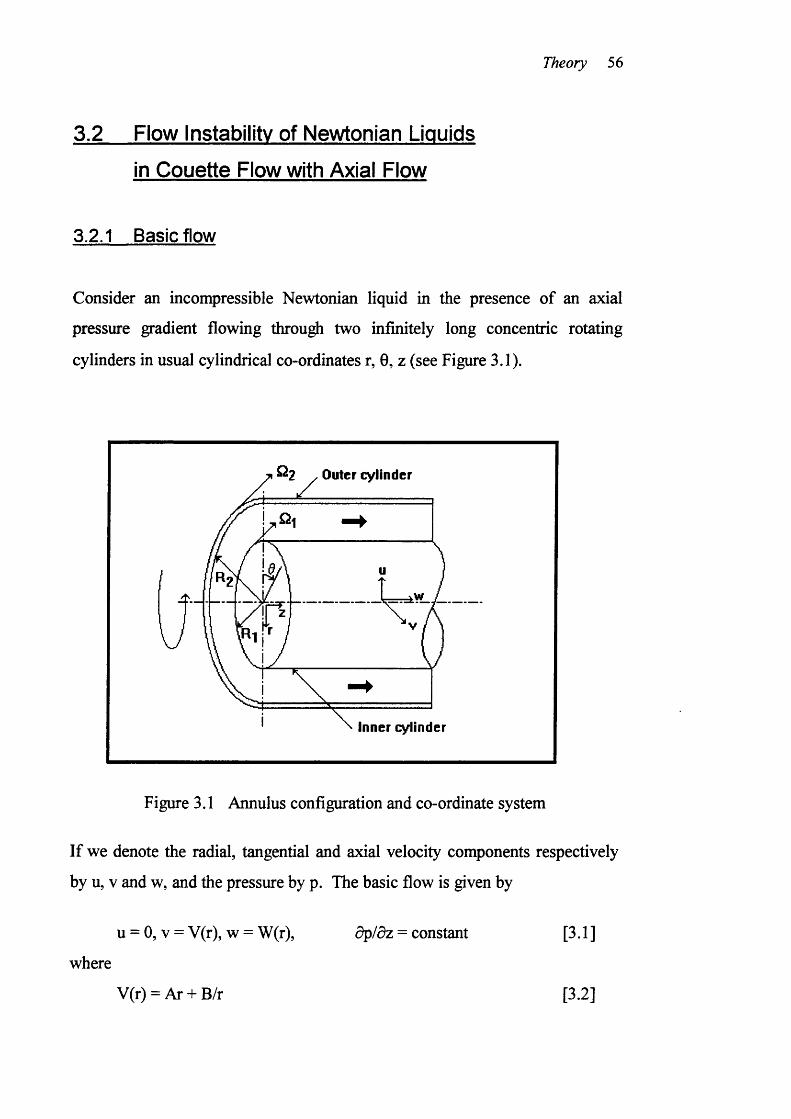
Theory 56
3.2 Flow Instability of Newtonian Liquids
in Couette Flow with Axial Flow
3.2.1 Basic flow
Consider an incompressible Newtonian liquid in the presence of an axial
pressure gradient flowing through two infinitely long concentric rotating
cylinders in usual cylindrical co-ordinates r, 0, z (see Figure 3.1).
Outer cylinder
inner cylinder
Figure 3.1 Annulus configuration and co-ordinate system
If we denote the radial, tangential and axial velocity components respectively
by u, V and w, and the pressure by p. The basic flow is given by
u = 0, V = V(r), w = W(r), d p i d z = constant
where
V(r) = Ar + B/r
[3.1]
[3.2]
Theory 57
[3.3]
where A and B are two constants which are related to the angular velocities Qi
and Q2 with which the inner and the outer cylinders are rotated. Thus, if Ri
and R2 (> Ri) are the radii o f the two cylinders, then we have
where
a = R1/R2 and p = Q2/
1-a^[3.4]
[3.5]
The average axial velocity, W , can be obtained by integrating of Eq. [3.3] with
respect tor. Thus:
1 + l - ( R i / R z ) : R2 J ln(R2 /R i)
[3.6]
where p is the kinematics viscosity. The Eq. [3.2] represents a circular Couette
flow while the Eq. [3.6] is the average Poiseuille flow in an annular gap.
3.2.2 Governing equations
Assuming the flow to be axisymmetric, the hydrodynamics equations governing
an incompressible Newtonian liquid in cylindrical polar co-ordinates (r, 0, z)
may be expressed in the following forms: (Bird, Stewart and Lightfoot, 1960)
at "ar az r " arlp ^a^u 1 au a^uar
a av av av uv 0 : "5T+U— + w — + — = +v
at ar ÔZ Ta^v 1 av a^v
[3.7a]
[3.7b]
Theory 58
dw dw , , ,at ar dz ~ & lp
aw afp^ ( a^w i aw a^w —-----1 H I J. \«------- 1-------- 1------rar a,2
and, the continuity equation: au u aw .
[3.7c]
[3.7d]
To study the instability o f this steady motion, we disturb the velocity field of
the Couette flow with small disturbances;
e.g. V = V + v' [3.8]
where the primed quantities denote small perturbations on the basic motion. It
is convenient to separate the flow into a mean part and a disturbance part,
where the latter has a zero mean. It is clear that the two parts of the flow are
interdependent through the action o f the Reynolds stress on the mean flow. On
the basis o f linear theory, the disturbance is assumed to be so small that the
effect o f the Reynolds stress on the mean motion can be neglected, in which
case the mean flow is the original laminar flow. Substituting these quantities
into the Navier-Stokes and continuity equations give
r:
z:
1 au' a^u' u*"'2 r ar a_2 _2ar'
a (v + V' + (V+ viu'at ar ÔZ
= V^a^(v + v') i a (v + v') a^cv + v') (v + v')"'------ 1--------r------ 1-------- --------V ar' ar az' r y
+ _ a (w + w ')at ar az a z lp
fa^(w + w') ia (w + w’) a^(w+w')^+ V - + T-------- - +
ar' ar az'
continuity equation: au' u' a (w + w') _
[3.9a]
[3.9b]
[3.9c]
[3.9d]
Theory 59
It is assumed that the disturbance velocities u', V, w’ to be small compared to
the mean velocity V and W, we can neglect their quadratic terms to linearise
those equations. We obtain the linearised Navier Stokes and continuity
equations
r:
0:
z:
o t or T d z,2.,d 1 d v ' d v' v'
— j ■ — - - ■ — ---------
2 r d r ^ 2 _2
A
d r ‘ d z^ r v
1 d w '
continuity equation: du' u’ d w '
[3.10a]
[3.10b]
[3.10c]
[3.10d]
An examination of these equations show that they allow a solution in normal
mode form
[3.11a] [3.11b] [3.11c] [3.1 Id]
where u,v,w and p are functions of r only and t is the dimensionless time. The
two parameters a and s in Eqs. [3.1 la-d] characterise the flow perturbations in
the axial direction. Their values determine the growth rate of the disturbance
and for a given flow rate and geometry they uniquely determine whether the
imposed perturbations will decay or be able to grow exponentially in time
leading to the formation of secondary flow in the form of Taylor vortices. The
axial wave number, a, characterise the form of the disturbance. For a spatially
bounded disturbance, a must be real. In addition, with the wave number
restricted to positive values the imaginary part o f the complex growth rate, s,
determines the stability (s < 0) or instability (s > 0) of the basic flow. The
condition s = 0 corresponds to the case of neutral stability.
Theory 60
Substituting Eqs. [3.1 la-d] into Bqs.[3.10a-d] give:
r:gggi(az St) 3ue‘(az st) 2V j(az-st) _ 1 5 j(az-st)
at 0z r ~ p d ! ^
1 ggi(az-st)^+ V ---------------- 1------------------ 1-------------------------------
. ar: r ar az , 2 ^
— 2V-isu + W iau vr
J(az-st)p dr
‘ I d 2 1 ^ Li(az-st)
for A + i l Adr rJ dr
u =' d f d i] r
dr \dr
a f a n 1 2 1 s lawarlar rJ J.2 “ .2 v v
I dpU H V — -----—
r p ar
D D * - a : + ^ - ^V V
lapu + V = — —
r p ar[3.12a]
where D and D* denote and respectively
0: aveit-^-^) ray i(az-st) ^at lar rJ"® az
( 1 a v e ' (^ -^ ) g 2-g i(a z -st) ~^i(az-st)^
2 " 7 & & ^2 ^dr-
. ~ T7T. .w f av V 1-isv + Wiav - 1 + — I u ei(az-st):3<v a^ 1 a 2 1
^ g ,2+ rar-" \ 2 ^i(az-st)
- is v + Wiav - D * Vu = v| d D * -a '
V = D * Yu [3.12b]
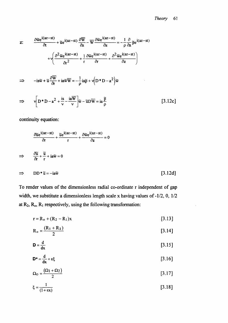
Theory 61
z: + ggi(az-st) ^ _ w 5 5 î!^ !L ^ = _lA%^i(az-st)W pe5t dz dz p dz
/ 1 ô2~gi(az-st)^2 r ar azar
a w 1 /-isw + u - ^ + iawW = — iap + v| d * D - a4w
D . D - a : + ^ - ^V V
w - ÏÏDW = ia— [3.12c]
continuity equation:
^ei(az-st) ggi(az-st) ^gi(az-st)+ + : = 0
ar dz
=> f + “ +iaw = 0 dr r
DD * u = -law [3.12d]
To render values o f the dimensionless radial co-ordinate r independent o f gap
width, we substitute a dimensionless length scale x having values of -1/2, 0, 1/2
at R2, Ro, Ri respectively, using the following transformation:
r — Ro 4- (R 2 — R i ) x
n _ (^1 + R2 ) R o - 2
D* = — + s£, dx
( Q 1 + Q 2 )
1(1 + 8X )
[3.13]
[3.14]
[3.15]
[3.16]
[3.17]
[3.18]
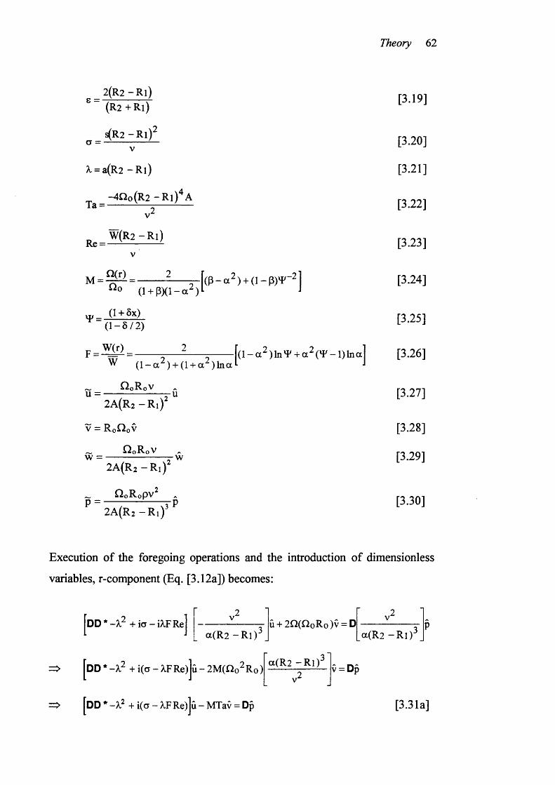
Theory 62
G =
a =
2 (R 2 -R i) (R2 + R i )
s( R 2 - R i )^
A, = a(R2 -R l)
—4 2o(R2 — Ri)^ATa =
Re = W(R2 - Rl)
M = Q(r) 2^0 (1 + PXl-a^)
(1 + ôx)
|(p -a 2 ) + (l-p)>p-2j
(1- 8 / 2)
f Æ =w (l-a ^ ) + (l + a^)lna
(l-a^ )lnY + a^(Y -l)lna]
u = QoRoV
2 A (R 2 - R l) '
V = RoQoV
u
w = QoRoV
2 A ( R 2 - R i )'w
QoRopv .
P = — :-----------3-p2A(Rz-Ri)^
[3.19]
[3.20]
[3.21]
[3.22]
[3.23]
[3.24]
[3.25]
[3.26]
[3.27]
[3.28]
[3.29]
[3.30]
Execution of the foregoing operations and the introduction of dimensionless
variables, r-component (Eq. [3.12a]) becomes:
a(R 2 - R l)
=> |dD * -')? + i(a - XFRe)jû - 2M(no^Ro)
=> ^DD*-X^ + i(o - XF Re)]û - MTav = Dp
Û + 2Q(QoRo)v = Da(R 2 - R l)'
a(R2 - Rl)' v = Dp
[3.31a]
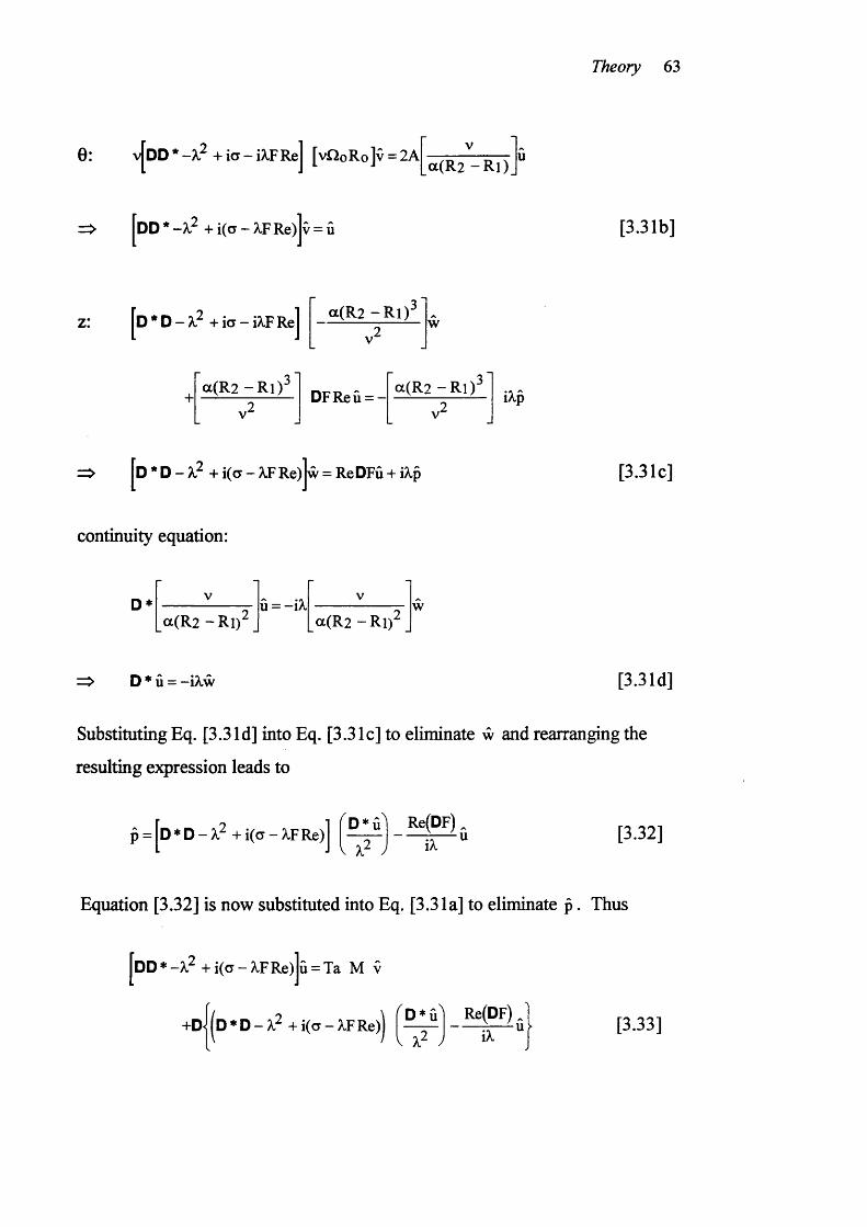
Theory 63
0: v [d D *-X ^ + io -iA F R e| [v£îoRo]v = 2Aa(R 2 - R l)
DD * - } ? + i(CT - A,FRe)|v = û [3.31b]
zi | d * D — + ÎG — ÎA.F Rej a(R2 - R l ) ' w
+ a(R 2 -R l)^ DFReû = - a (R 2 -R l)^
[ v2 J L v2 JiXp
=> | d *D-A.2 +i(a-X FR e)Jw = ReDFû + a p
continuity equation:
[3.31c]
D*a(R 2 - Rl)'
Û = -iA,a(R 2 - Rl)'
w
=> D * Û = -iAw [3.31d]
Substituting Eq. [3.3 Id] into Eq. [3.31c] to eliminate w and rearranging the
resulting expression leads to
P = D *D -X ^ +i(cr-XFRe)^D »ûl Re(DF)
iX[3.32]
Equation [3.32] is now substituted into Eq. [3.31a] to eliminate p . Thus
DD*-A^ +i(CT-AFRe) û = Ta M V
+d | | d ♦ D - + i(CT - AF Re)J D*Û^
V A V
Re(DF)iX
[3.33]
Theory 64
It is assumed that the concentric rotating cylinders between which the liquid is
contained are of rigid material and that no slip occurs at the surfaces o f contact.
In addition to the relation D ♦ û = -iA,w (Continuity equation), the three pairs of
boundary conditions are expressed as:
û = Dû = v = 0 at X = ±1/2 [3.34]
The homogeneous system o f Eqs. [3.31b] and [3.33] coupled with the boundary
conditions [3.34] define an eigenvalue problem with the eigenvalue Ta. The
flow is unstable or according as there are or are not solutions for which the
imaginary part o f dimensionless growth rate, a, is negative. In the present
study, we consider only the neutrally stable, imaginary part o f a equals to zero.
When the axial Re number equals to zero, we have the classic Taylor (1923)
problem and the eigenvalue problem will reduce to the case of pure Couette
flow which has been discussed in Section 2.2.1. Moreover, as in many
investigations of the linear stability theory, the complicated eigenvalue problem
can be simplified by considering the case when the gap between the cylinders is
small compared to their mean radius. So that, radius ratio, a tends to 1, D*
tends to D and the operator DD* reduces to D appropriate to the narrow-gap
configuration, as following equations, considered by Chandrasekhar (1961)
which has also been considered in Section 2.2.3.
+ i(CT - XFRe)jv = û [3.35]
-X ^ +i(CT-XFRe)Jû = Ta M v
+d | ( d +i(a-W Re)) [3.36]
In our present study, the eigenvalue problem will be solved without
simplification as in Eqs. [3.35] and [3.36] so that the restriction to narrow-gap
is lifted.
Theory 65
3.2.3 Method of solution
The eigenvalue problem defined by Eqs. [3.31b] and [3.33] is difficult to treat
analytically. An obvious choice for a numerical procedure is the Galerkin's
method. The principle o f the Galerkin method is given in Appendix 1.
Basically, this method consists o f expanding û and v in sets of complete
functions (trial function) that satisfy the boundary conditions. The coefficients
in the trial function series are determined by the requirement that the errors in
Eqs. [3.31b] and [3.33] be orthogonal to the expansion functions (weighting
function) for û and v , respectively. This leads to a system o f infinitely many
linear, homogeneous equations for the coefficients in the series. For a non
trivial solution it is necessary that the determinant for the system of equation
vanishes, and this gives a determinantal equation for Taylor number. In
practice only a finite number o f terms are used in the series for û and v , say N,
and this leads to a determinant of size 2N.
According to Galerkin method, there is no restrictions on the form of the trial
function unless they satisfy the boundary conditions (Eq. [3.34]). In our study,
there is a number of possible sets o f complete functions which can be used for
the expansions o f û and v . For example, the set of functions sin(2n-I)7cx and
cos2n7ix (n = I, 2,....) could be used for v , and the set of functions Cn and Sn
tabulated by Harris and Reid (1964) could be used for û . Unfortunately, the
choice of trigonometric functions leads to a prohibitive amount of labour just to
evaluate the entries that appear in the determinantal equation. Indeed it is not
clear that many o f the integrals can even be evaluated in closed form.
For our purposes it is more convenient, to use simple polynomials in x that
satisfy the boundary conditions. Thus we choose
00 00
U = ^anUn and V = ^bnVn [3.37]n=l n=I
Theory 66
where
Un =n-1 and V n = X X
n-1 [3.38]
Here and bn are unknown coefficients which are yet to be determined. One
can now introduce the concept o f an error function by substitution of Eq. [3.37]
in Eqs. [3.31b] and [3.33] respectively. The expression Ei and E? represent
the errors occurring in the domain or on the boundary due to non-satisfaction of
the above equation. The error functions are given by
| d D*-A,^ + i ( a - À F R e ) ] ^ anUn - Ta M ^ bnVnn=l n=l
—d I^ D * D — + i(a — X,FRe)j f — anUn[ V ^ n=l -
R e ( D F ) ^ 1 ^/ , anUn = EliX
[3.39a]n=l
P , N N[DD * — + i(g — A .F R e ) J b n V n ~ anUn = £ 2
n=l n=l
where n = 1, 2,...., N
[3.39b]
In this case the weighting functions are, Um and Çv , where Ç is the appropriate
wei^ting function for DD* given by
1(1 + Ex)
where
2(R2 - R l)
(R 2 + R i)
[3.40]
[3.41]
m = l, 2,..., N
Theory 67
Then, multiplying [3.39a] by Çum and [3.39b] by Çvm for m = 1, 2,...., N, and
integrating from -1/2 to +1/2. The weighted error expressions are
N
n=lan
1/2 1/2 R fi/DF'IJ^Um|DD * + i ( c - XFRe)]undx - J^um — — Un
- 1/2
1/2
- 1/2
- 1/2
— j* ^UmD |d * D — + i ( c — XFRe)j ( —— Un
-b n T a M j^^^^^UmVndx = 0 [3.42a]
"1/2 ■
E an J^VmUndx — bnn=l --1/2
1/2
J^Vm^DD * -X^ + i(CT - XFRe)jvndx
- 1/2
= 0 [3.42b]
m = 1, 2 ,...., N
The subsequent solution procedure consists of solving the linear algebraic
homogeneous equations [3.42a-b] for given radius ratio, a, angular speed ratio,
P, Reynolds number. Re and increasing N (beginning with N = 1) by equating
the real and imaginary parts o f their determinant to zero to yield a non-trivial
solution. For N = 1, a systematic searching technique is employed which, for
given dimensionless growth rate, a, yields a real positive root for Taylor
number, together with the corresponding value of dimensionless wave number,
X. The minimum Ta number over a range of a is taken as the approximation to
critical Ta number together with the associated values of X and a.
For the large-size determinants (N = 4) the procedure differed somewhat in
that, for given a, P, Re and X, a is so chosen that the value of Ta number for
which the secular determinant vanished is real; a is then varied to determine the
minimum positive real value of critical Ta number which, in turn, is minimised
over all real positive X. All computation are programmed in Mathematica
software as given in Appendix 2.
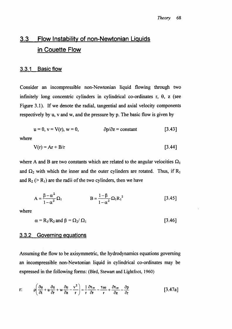
Theory 68
3.3 Flow Instability of non-Newtonian Liquids
in Couette Flow
3.3.1 Basic flow
Consider an incompressible non-Newtonian liquid flowing through two
infinitely long concentric cylinders in cylindrical co-ordinates r, 0, z (see
Figure 3.1). If we denote the radial, tangential and axial velocity components
respectively by u, v and w, and the pressure by p. The basic flow is given by
u = 0, V = V(r), w = 0, d ^ l d z = constant [3.43]
where
V(r) = Ar + B/r [3.44]
where A and B are two constants which are related to the angular velocities Qi
and Q2 with which the inner and the outer cylinders are rotated. Thus, if Ri
and R2 (> R l) are the radii of the two cylinders, then we have
A = -& -Î^ Q i B = [3.45]
where
a = R1/R2 and P = Q2/ 0% [3.46]
3.3.2 Governing equations
Assuming the flow to be axisymmetric, the hydrodynamics equations governing
an incompressible non-Newtonian liquid in cylindrical co-ordinates may be
expressed in the following forms: (Bird, Stewart and Lightfoot, 1960)
= [3.47a]T dr r dz dr
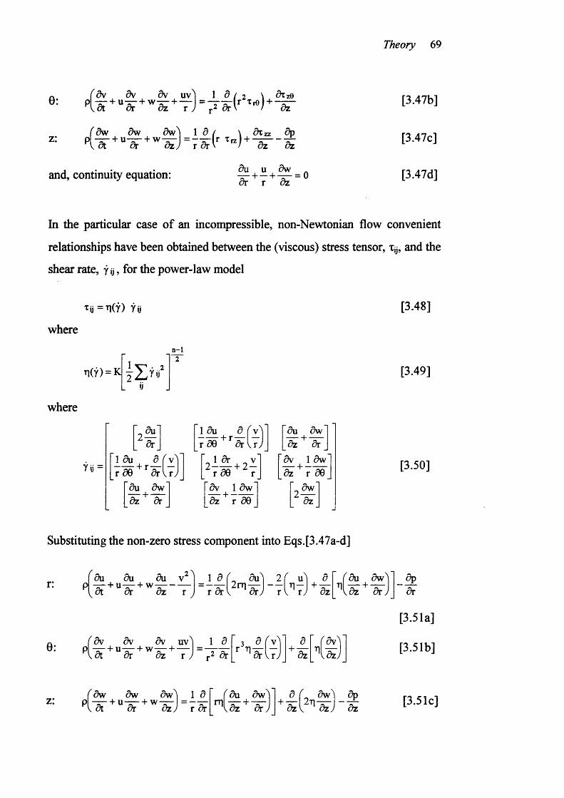
Theory 69
0: ôw dw dw MW I d ( 2 \ , àzzQdt ' dr ' d z ^ T ) ôrV dz(r^rt)
f dw dw 1 ^ / \ dizz dpp l - â r + " - & 4 + ^ - %
and, continuity equation:
[3.47b]
[3.47c]
[3.47d]
In the particular case o f an incompressible, non-Newtonian flow convenient
relationships have been obtained between the (viscous) stress tensor, Xÿ, and the
shear rate, ÿ ÿ, for the power-law model
'Tij =Tl(Ÿ) ÿij
where
n(ÿ) = K l l r .
n-1~2~
where
Yij = r 505u dw d z ^ dr
d~^^dr (t)]
1 5u d fw
4 # - 4dw 1 dw% +7-æ
5u dw~didw 1 dw
dw
[3.48]
[3.49]
[3.50]
Substituting the non-zero stress component into Eqs.[3.47a-d]
r:
0:
5u 5u 5u V — + u — + w — - -
2 \ 5u dw
5v 5v 5v uvPI aT
1 d 3 d d ' f^ VJ.2 dr ^ dz
dr
[3.51a]
[3.51b]
f dw dw dw i Ar dr
f dû dw [3.51c]
Theory 70
Similar to Section 3.2, small disturbances are added the velocity field of the
Couette flow in order to study the stability of this steady motion
e.g. V = V + v' [3.52]
Substituting these quantities into the Navier-Stokes and continuity equations
gives
r: du', ,au' ,gu' (v+v'yd t ^ d z r
2_ar dr r ( T i + T | ' ) ~d^
2 ,_ ddr [3.53a]
0: d(V + v') ,d(V + v') ,a(V + v') (V + v'X+ U _------ + W _----- -4-d t dr d z
j _ _ a
r: a-+ d z (n + Ti')l^(v+v’) [3.53b]
z: d w ' dw ' dw ' _ ^ r du' dw'^~d^_ r dr . d z ^
[3.53c]
continuity equation:
u ’ d ^ ' [3.53d]
It is assumed that the disturbance velocities u', v% w' to be small compared to
the mean velocity V, we can neglect their quadratic terms to linearise those
equations. We obtain the linearised Navier Stokes and continuity equations
r: d i r
d du 2 du! — ^du dr\ 2\xv[
— d du! — d d w ' du' [3.55a]
Theory 71
0:'dw' ,av ,va ar r
1 a r 3 _ a (wYl _ a av'_ " r : ar [3.55b]
aw' a —/"au' aw'^ 1 _/"au' aw'l a — aw'z: p“aT "ar
+ - r 5-^^-arJ_ dz - f [3.55c]
continuity equation: au' u' aw' [3.55d]
An examination of these equations show that they allow a solution in normal
mode form
u'=ue^
w = we p’=pe*“
[3.56a][3.56b][3.56c][3.56d]
where u,v,w and p are functions of r only. Substituting Eqs. [3.56a-d] into
Eqs. [3.55a-d] gives:
r: aue*“ 2Vat ve a aue‘“ 2%
r arag arj iaz 2r|ue‘ ar ar
_ a aiïe^ _ a awe^ ape'ar
- ^ vr = 2t]DDu-i-—Dut] + 2DuDt| - - -H t]u + ia^Dw - Dp [3.57a]r
where
D = —ar
0: 1 ar2 ar ■’" 'It'*"
av Var r + a T|v
Theory 72
"av Var r
u = nu r ar
p[D * V]u = T[|nDD * -a^ j v + n[Dr[]D v
V 2 —~ , "a r " a n "
7 - a T]v + na r r
Va r
[3.57b]
where
'a w e ^ ' a faue‘“ a w e ^ lz: P at "ar az dr ^ + d z
1+ -r
aue*“ awe +
ÔZ drape*
d z
- I_ —awr j iA u + T] — + -^2A, t]w + — d z r
_ _awT11ÀU+T1 — -iÀp
0 = iA,T|Du + iA,uDri + t|DE>w + DwDti + 2A, t|w+ —iA,T)u+ —t|E)w - i?ip [3.57c]
continuity equation:
aïïe*“ ue*“ awe*“ ^
— H— + l a w = 0 a r r
DD*u = -iaw [3.57d]
To render values of the dimensionless radial co-ordinate r independent of gap
width, we substitute a dimensionless length scale x having values of -1/2, 0, 1/2
at R2, Ro, Rl respectively, using the following transformation:
r — R q 4- ( R 2 — R l ) x
Ro = (R, ~"R )
[3.58]
[3.59]
Theory 73
D* = — + dx
D = - — dx
Ho =(Q l + 0 2 )
4 =
E =
1(1 + Ex)
2(R2 - R l)
(R 2 + R l)
< R 2-R i )
"k = a(R2 - R l)
-4p^O o(R z — R l) ATa =
M =
Mm
Q(r) 2
(1 + PXl-a^)
(1 + 5x)
( P -a ^ ) + ( l -P )Y -2
(1 -5 /2 )
P _ _n_ _ (2 - nXl - p) j-j2/n-l Pm
n= (1 + Ôx)(1 + 5 / 2 )
n = K K2 .2/n
n—1
R2
Pm =( R 2 -R .)
Rl
K K2
n-1
1R 2 — Rl
K2 =2(0: -ni)R2^'°
n[(R2 /R i) ^ '° - l
[3.60]
[3.61]
[3.62]
[3.63]
[3.64]
[3.65]
[3.66]
[3.67]
[3.68]
[3.69]
[3.70]
[3.71]
[3.72]
[3.73]
[3.74]
[3.75]
Theory 74
u =QoRoV
2 A ( R 2 - R i)'
V = RoQoV
u
w = OoRoV2A(R2-Riy
w
Q o R o p v .P — , . 3 P
2 A ( R 2 - R , f
[3.76]
[3.77]
[3.78]
[3.79]
Execution o f the foregoing operations and the introduction of dimensionless
variables, r-component (Eq. [3.57a]) leads to:
—2f2(OoRo )p^a(R2 - R l)
V = 2PDDÛ + 204DÛP + 2DÛDP - 2Ô ^ ÛP
-l^PÛ + iXPEXv-Dp
MTav = [P(D + Ô4)DÛ - P6^^^Û + iÀPDw] + p[dD + Ô D - ]û
+2DÛDP-2À^PÛ-Dp
MTav = [p(d * D - 52^2 J- ^ iKPD^^ + p[dD * ]û + 2DÛDP - Dp
MTav = [PDD * û + iA,PDw] + p[üD * ]û + 2DÛDP - Dp
MTav = PD[D * û + iÀw] + p[dD * - X ^ ]û + 2DÛDP - Dp
p[dD *-X ^]û +2DÛDP = MTav + Dp [3.80a]
0: p2A gmpa(R2 - R l)
u = PmP(R 2 - R l) '
[nDD*-A.^l [£2„Ro]v + nDgmPD^(R2 — Ri)^
[QoRo]i
P^nDD * -X^ jv + nDpmPD^ v = û [3.80b]
Theory 75
z: 0 = iXPDû + iXûDP + PDDw + DwDP - 2X^Pw + S iXPû + 5ÇPDw - iXp
0 = iXP[D + 8^]û - X^Pw + P[D + SÇ]Dw - X PW + DPD^ + DPiXû - iXp
0 = iXP[D * û + iXw] + p Fd * D - xMw + DP[Dw + iXÛ] - iXp
p [d * D - X |w + DP[Dw + iXû] - iXp = 0 [3.80c]
continuity equation:
D* P<mpot(R2 — Rl)"
Û = -iA, M-m
pa(R2 — Ri)w
D * û = -iAw [3.80d]
Substituting Eq. [3.80d] into Eq. [3.80c] to eliminate w and rearranging the
resulting expression leads to
p = i [ 0 * D - X ^ ] D»Û + [D D * Û + Û] [3.81]
Equation [3.81] is now substituted into Eq. [3.80a] to eliminate p . Thus
p [d D*-A^]û +2DÛDP = M Ta v + d J ^ D * D D * û - PD * Û
+ ^ D D » û + û [3.82]
If we assume that the rotating cylinders between which the liquid is contained
are of rigid material and that no slip occurs at the surfaces of contact. In
addition to the relation D*û = -iAw (continuity equation), the three pairs of
boundary conditions are expressed as:
Û = Dû = V = 0 at X = ±1/2 [3.83]
Theory 76
3.3.3 Method of solution
The homogeneous system of Eqs. [3.80b] and [3.82] coupled with the boundary
conditions (Eq. [3.83]) define an eigenvalue problem with the eigenvalue Ta
number. When flow index, n, equals to unity, we have the classic Taylor
(1923) problem which has been discussed in Sections 2.2.1.
The conditions o f the stability limit o f the Couette flow with the power law
viscosity are described by the critical Ta number, Ta , being a function of
parameters: radius ratio, a, angular speed ratio, P and the flow index, n. All
eigenvalues Ta number of the Eqs. [3.80b], [3.82] and [3.83] are real. The set
of the smallest positive values Ta number determined at the given values of
dimensionless wave number, A,, defines the neural curves o f Ta number. The
minimum of the function Ta number at a given a, p, and n determines the
critical Ta number and the dimensionless wave number,
For our purposes it is convenient to use the Galerkin method as a simple
polynomials in x that satisfy the boundary conditions. Thus we choose
00 00
Û = ^anUn and V = ^bnVn [3.84]n=l n=l
where
2 1 _ r ..2 l _.n—1U n= |x"-^ l and V n=lx^-^ |x“- [3.85]
Here a and bn are unknown coefficients which to be determined. One can now
introduce the concept of an error function by substitution o f Eqs. [3.84] in
[3.80b] and [3.82] respectively. The expression Ei and Eo represent the errors
occurring in the domain or on the boundary due to non-satisfaction of the above
equation. The error functions are given by
Theory 11
p [d D * -X ^ ]2 ] a „ U n -T a M ^ b „ v „ - d | - ^ ( d * D -A .^ ) D * ^ a .u .n=l n=I n=l
D P (D D * + 1 )^ 1.2 [3.86a]
n=l
( X 1 \ N N|p[nDD*-X2] + nD^mPD'^|^ b n V n -^ anUn=E2
n=l n=l
[3.86b]
where n = 1, 2,...., N
In this case the weighting functions are, Um and Vm, where % is the appropriate
weighting function for DD* given by
1(1 + 8 X )
where
s =2 ( R 2 - R i ) (R 2 + R i )
[3.87]
[3.88]
m = l , 2,..., N
Then, multiplying [3.86a] by Çum and [3.86b] by for m = 1, 2,...., N, and
integrating from -1/2 to +1/2. The weighted error expressions are
N
n=l
Sin
1/2 1/2 r
J^UmP|DD*-A,^Jundx- J ^UmD — JD*D-A,^J D*Un- 1/2 - 1/2
DP(DD‘ +1) , I f/2 r,Um — Un -b n T a M| ÇUmVn- j ,
- 1/2
dx = 0 [3.89a]
Theory 78
N ' 1/2
z a n J ^ V m U n d x — b on=l - - 1/2
1/2
|4vm {p[nDD * -^^] + nDn„PD*|v„dx- 1/2
= 0
[3.89b]
m = 1, 2 , N.
Equations [3.89a-b] represent a doubly infinite set of linear homogeneous
equations in the variable a and bn for given radius ratio, a, angular speed ratio,
P, flow index, n and N. By setting the determinant of the system equal to zero,
we obtain the required eigenvalue problem for Ta number. All computation are
programmed in Mathematica software as given in Appendix 3.
Materials and Methods 79
CHAPTER FOUR
MATERIALS AND METHODS
4.1 Introduction
The main objective of the present experimental study is to determine the
residence time distribution (RTD) o f a range of Newtonian and non-Newtonian
liquids flowing through the annular gap of a Couette flow device. The
experiments were carried out by using a stimulus response technique based on
an impulse input to characterise the transition from Couette flow to Taylor-
Couette flow regime. A general arrangement of the experimental set-up is
shown in Fig. 4.1. In Section 4.2, equipment of the present study will be
described. It includes concentric cylindrical apparatus, sensors associated with
the Couette flow device and the viscosity measuring device. In Section 4.3, a
rheological properties and the preparation of a range of Newtonian and non-
Newtonian liquids and their corresponding tracer solutions will be described in
details. Finally, the experimental methods associated with the determination of
the RTD and the technique for obtaining experimental data by using the data
acquisition system will be discussed in Section 4.3.
4.2 Equipment
4.2.1 Couette flow device
A Couette flow device of the present study basically consisted of a stationary
outer shell and a rotating inner cylinder with an axial length of 1000 mm. The
diameter of inner cylinder was less than that of the shell giving a horizontal
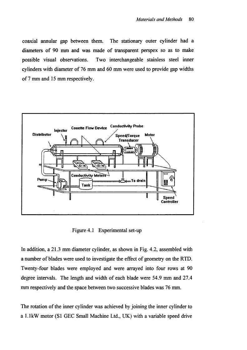
Materials and Methods 80
coaxial annular gap between them. The stationary outer cylinder had a
diameters o f 90 mm and was made o f transparent perspex so as to make
possible visual observations. Two interchangeable stainless steel inner
cylinders with diameter of 76 mm and 60 mm were used to provide gap widths
of 7 mm and 15 mm respectively.
Conductivily ProbeCouette Flow DeviceInjectorDistributor SpeedfTorque Motor
T ransducer \
Conductivity M eterPump
Tank
SpeedController
Figure 4.1 Experimental set-up
In addition, a 21.3 mm diameter cylinder, as shown in Fig. 4.2, assembled with
a number o f blades were used to investigate the effect of geometry on the RTD.
Twenty-four blades were employed and were arrayed into four rows at 90
degree intervals. The length and width of each blade were 54.9 mm and 27.4
mm respectively and the space between two successive blades was 76 mm.
The rotation of the inner cylinder was achieved by joining the inner cylinder to
a 1.1 kW motor (SI GEC Small Machine Ltd., UK) with a variable speed drive
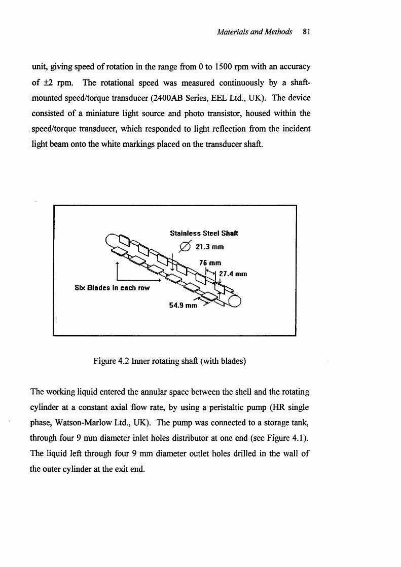
Materials and Methods 81
unit, giving speed of rotation in the range from 0 to 1500 rpm with an accuracy
of ±2 rpm. The rotational speed was measured continuously by a shaft-
mounted speed/torque transducer (2400AB Series, EEL Ltd., UK). The device
consisted of a miniature light source and photo transistor, housed within the
speed/torque transducer, which responded to light reflection from the incident
light beam onto the white markings placed on the transducer shaft.
Stain less Steel Shaft
21.3 mm
76 mm27.4 mm
Six Blades in each row
54.9 mm
Figure 4.2 Inner rotating shaft (with blades)
The working liquid entered the annular space between the shell and the rotating
cylinder at a constant axial flow rate, by using a peristaltic pump (HR single
phase, Watson-Marlow Ltd., UK). The pump was connected to a storage tank,
through four 9 mm diameter inlet holes distributor at one end (see Figure 4.1).
The liquid left through four 9 mm diameter outlet holes drilled in the wall o f
the outer cylinder at the exit end.
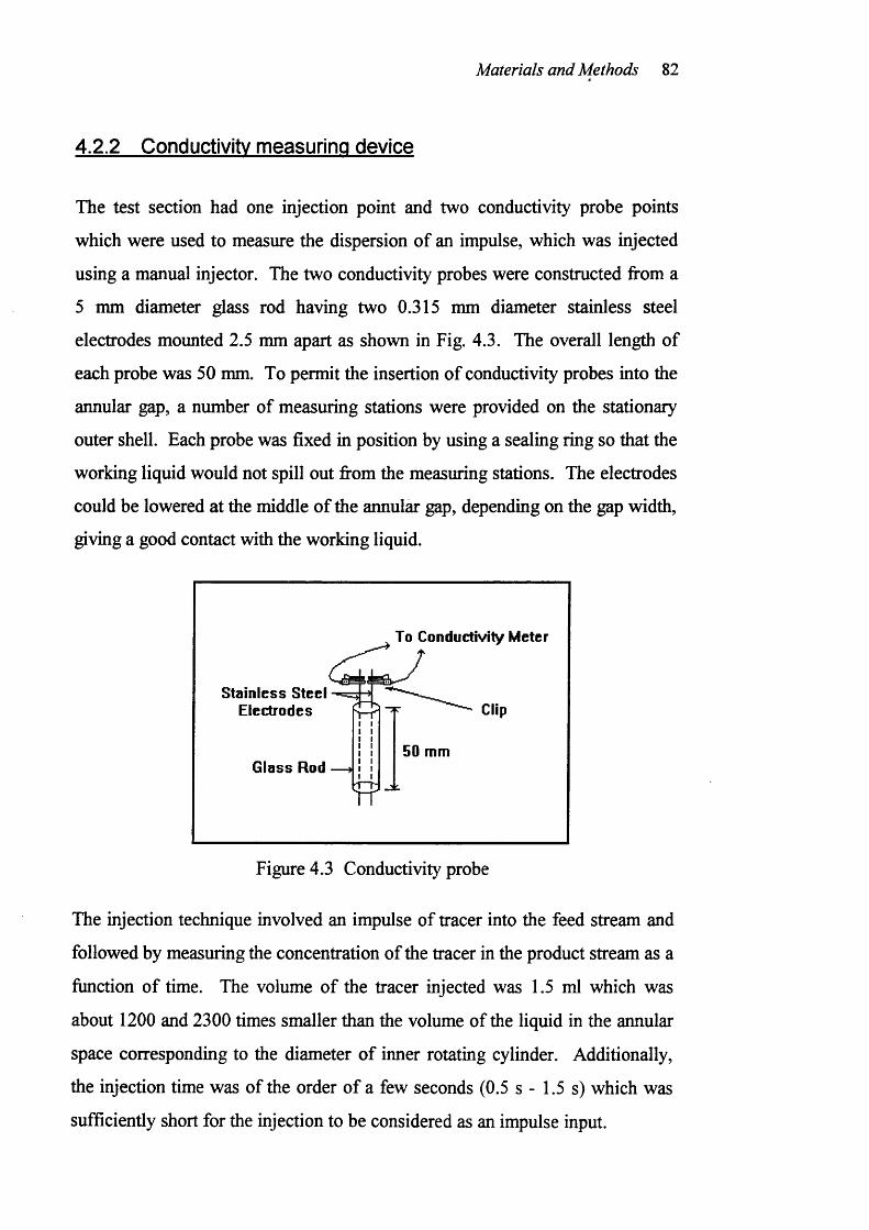
Materials and Methods 82
4.2.2 Conductivity measuring device
The test section had one injection point and two conductivity probe points
which were used to measure the dispersion of an impulse, which was injected
using a manual injector. The two conductivity probes were constructed from a
5 mm diameter glass rod having two 0.315 mm diameter stainless steel
electrodes mounted 2.5 mm apart as shown in Fig. 4.3. The overall length of
each probe was 50 mm. To permit the insertion of conductivity probes into the
annular gap, a number of measuring stations were provided on the stationary
outer shell. Each probe was fixed in position by using a sealing ring so that the
working liquid would not spill out from the measuring stations. The electrodes
could be lowered at the middle o f the annular gap, depending on the gap width,
giving a good contact with the working liquid.
To Conductivity Meter
Stainless Steel Electrodes Clip
50 mmG lass Rod
Yr
Figure 4.3 Conductivity probe
The injection technique involved an impulse of tracer into the feed stream and
followed by measuring the concentration of the tracer in the product stream as a
fimction of time. The volume of the tracer injected was 1.5 ml which was
about 1200 and 2300 times smaller than the volume of the liquid in the annular
space corresponding to the diameter of inner rotating cylinder. Additionally,
the injection time was of the order of a few seconds (0.5 s - 1.5 s) which was
sufficiently short for the injection to be considered as an impulse input.
Materials and Methods 83
In order to provide an injection without leakage as the injector was removed
from its port, a small circular piece of silicon "self sealing" compound was
placed inside the injection station.
Two identical conductivity meters (CM35, WPA Co. Ltd., UK) were used to
detect the conductivity of tracer in the liquid passing through. These portable
meters were designed for routine laboratory and research measurements. Their
operating range was suitable for direct readings of conductivity between O.lp
siemen and Ip siemen and have an accuracy of ±3%. This allowed a wide
range of readings to be taken with a single cell. The conductivity measurement
versus time data were plotted and stored in a data-acquisition system for
subsequent analysis.
4.2.3 Viscosity measuring device
A standard coaxial cylinder (Contraves Rheomat 115, Contraves GmbH,
Germany) viscometer was used for the rheological measurements. The
Contraves has been used for many years as a research viscometer because of an
extensive shear rate range, high accuracy. Figure 4.4 shows an exploded view
of the sample holder from the Contraves viscometer.
The measuring bob was driven by an electromotor. The braking torque exerted
on the bob was measured in the measuring head of Rheomat 115 and indicated
on the control panel. The (shearing) speed and the shear stress were used to
obtain the rheological behaviour.
Principally, the data collected during rheological measurements were placed on
a spreadsheet for conversion from torque readings (N.m) and rotational speeds
(rpm) to the more useful rheological measurement units, i.e. the shear rates
(1/s) and shear stresses (Pa). The spreadsheet used was Lotus Corporation's
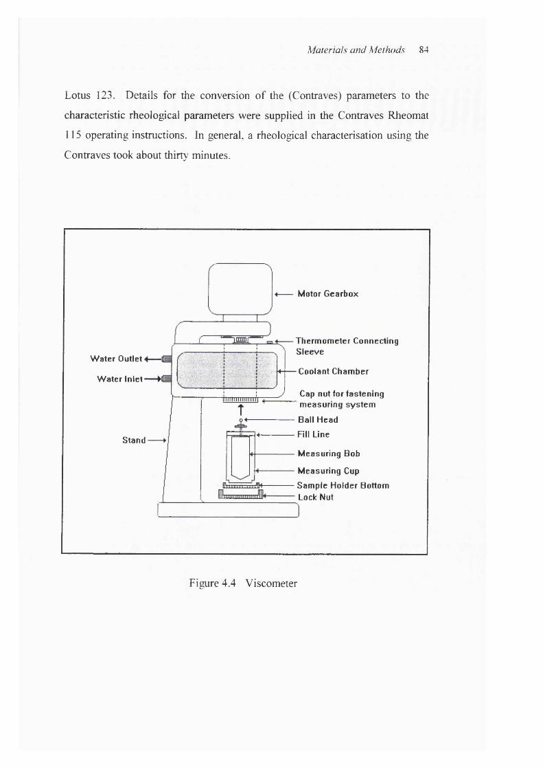
Materials and Methods 84
Lotus 123. Details for the conversion of the (Contraves) parameters to the
characteristic rheological parameters were supplied in the Contraves Rheomat
115 operating instructions. In general, a rheological characterisation using the
Contraves took about thirty minutes.
rW ater Outlet ■
W ater Inlet g
Stand
nr inm i i i i i inT TÎ i---
Motor Gearbox
Therm om eter Connecting S leeve
Coolant Cham ber
Cap nut for fas ten ing m easuring sy s te m
Ball Head
Fill Line
M easuring Boh
M easuring Cup
Sam ple Holder Bottom Lock Nut
Figure 4.4 Viscometer
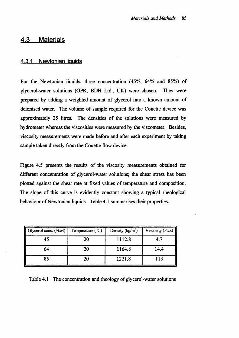
Materials and Methods 85
4.3 Materials
4.3.1 Newtonian liquids
For the Newtonian liquids, three concentration (45%, 64% and 85%) of
glycerol-water solutions (GPR, BDH Ltd., UK) were chosen. They were
prepared by adding a weighted amount of glycerol into a known amount of
deionised water. The volume o f sample required for the Couette device was
approximately 25 litres. The densities o f the solutions were measured by
hydrometer whereas the viscosities were measured by the viscometer. Besides,
viscosity measurements were made before and after each experiment by taking
sample taken directly from the Couette flow device.
Figure 4.5 presents the results o f the viscosity measurements obtained for
different concentration of glycerol-water solutions; the shear stress has been
plotted against the shear rate at fixed values o f temperature and composition.
The slope o f this curve is evidently constant showing a typical rheological
behaviour o f Newtonian liquids. Table 4.1 summarises their properties.
Glycerol conc. (%wt) Temperature (°C) Density (kg/m ) Viscosity (Pa.s)
45 20 1112.8 4.7
64 20 1164.8 14.4
85 20 1221.8 113
Table 4.1 The concentration and rheology of glycerol-water solutions
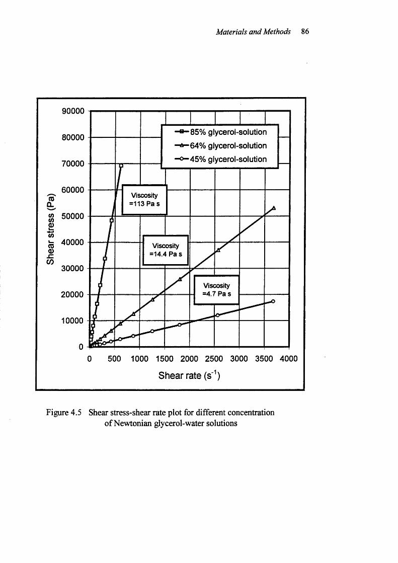
Materials and Methods 86
(0û .
IIs zCO
90000
85% glycerol-solution
64% glycerol-solution
45% glycerol-solution
80000
70000
60000Viscosity =113 Pa s
50000
40000 Viscosity =14.4 Pa s
30000
Viscosity =4.7 Pa s20000
10000
0500 1000 1500 2000 2500 3000 3500 40000
Shear rate (s' )
Figure 4.5 Shear stress-shear rate plot for different concentrationof Newtonian glycerol-water solutions
Materials and Methods 87
4.3.1 non-Newtonian liquids
The following is a brief summary of some of the unusual effects exhibited by
non-Newtonian liquids. It is presented in order to acquaint the reader with the
type of material being considered and also to establish some nomenclature.
For most practical purposes we can regard rheology as the study of liquids that
do not obey Newton's law o f viscosity. This law says in effect that:
• the only stress generated when a liquid flows - ignoring inertia - is the
shear stress;
• this shear stress is directly proportional to the shear rate, and thus the
viscosity (the shear stress divided by the shear rate) is constant;
• shear stress appears and disappears instantaneously when the flow
starts or stops.
The viscosity p is then given by
T = p y [4.1]
where x and ÿ are the shear stress and shear rate respectively. Figure 4.6
indicates that a plot o f shear stress against shear rate is a straight line through
the origin with slope equal to the viscosity of a Newtonian liquid, p. Most
liquids of simple structure, composed of relatively simple molecules in a single
phase, behave as Newtonian liquids, e.g. water.
However, in non-Newtonian liquids stresses other than the shear stress can
appear. These, together with the shear stress, are rarely linearly related to the
shear rate, and they neither appear nor disappear instantaneously on start-up or
cessation o f flow.
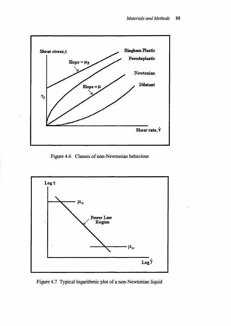
Materials and Methods 88
Bin^am Plastic
PseudoplasticShear stress,!
Slope = |lp
Newtonian
DilatantSlope =
Shear rate, T
Figure 4.6 Classes o f non-Newtonian behaviour
Log!
X
Power Law Region
00
Logÿ
Figure 4.7 Typical logarithmic plot of a non-Newtonian liquid
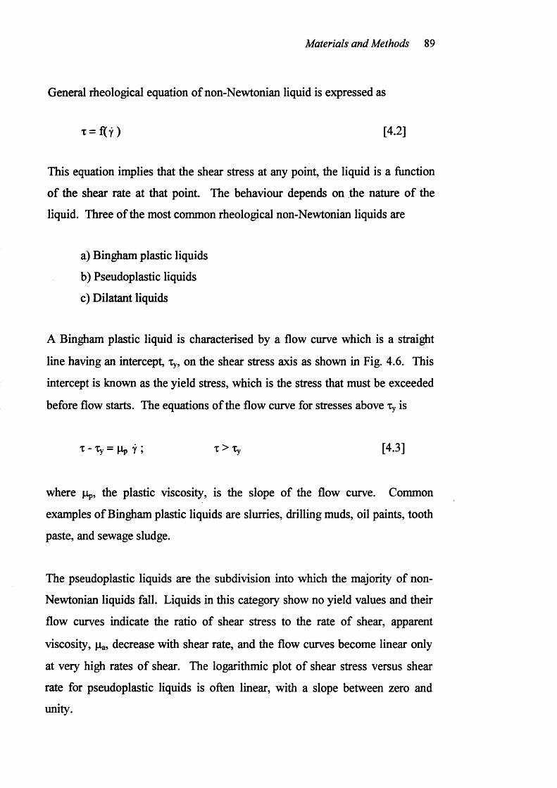
Materials and Methods 89
General rheological equation o f non-Newtonian liquid is expressed as
T = f (y ) [4.2]
This equation implies that the shear stress at any point, the liquid is a function
o f the shear rate at that point. The behaviour depends on the nature o f the
liquid. Three o f the most common rheological non-Newtonian liquids are
a) Binÿiam plastic liquids
b) Pseudoplastic liquids
c) Dilatant liquids
A Bingham plastic liquid is characterised by a flow curve which is a straight
line having an intercept, Xy, on the shear stress axis as shown in Fig. 4.6. This
intercept is known as the yield stress, which is the stress that must be exceeded
before flow starts. The equations o f the flow curve for stresses above Xy is
x-Xy = Ppÿ; x>Xy [4.3]
where Pp, the plastic viscosity, is the slope of the flow curve. Common
examples o f Bingham plastic liquids are slurries, drilling muds, oil paints, tooth
paste, and sewage sludge.
The pseudoplastic liquids are the subdivision into which the majority of non-
Newtonian liquids fall. Liquids in this category show no yield values and their
flow curves indicate the ratio of shear stress to the rate o f shear, apparent
viscosity, pa, decrease with shear rate, and the flow curves become linear only
at veiy high rates o f shear. The logarithmic plot o f shear stress versus shear
rate for pseudoplastic liquids is often linear, with a slope between zero and
unity.
Materials and Methods 90
A typical viscosity curve for non-Newtonian liquid is shown in Fig. 4.7. As
can be seen from this figure, three distinct regions are present. At very low
rates of shear the viscosity approaches Po the "zero-shear viscosity". For
extremely high shear rates, the "upper limit viscosity", pœ, is approached. The
intermediate region is characterised by a viscosity which decreases with shear
rate, a phenomenon referred to as pseudoplastic liquid. The familiar "power
law" viscosity model is frequently found to apply in this region. An empirical
functional relation is given by
t =Ky “ [4.4]
where consistency index, K, corresponds to the viscosity o f the liquid; flow
index, n, is the power law describes three flow models.
1) Pseudoplastic, n < 1
2) Newtonian, n = 1
3) Dilatant, n > 1
Examples of pseudoplastic liquids include melts (rubbers, cellulose acetate),
mayonnaise, gelatine, clay, milk, blood and liquid cement.
Dilatant liquids display a rheological behaviour opposite to that of
pseudoplastic, in that the apparent viscosity increases with increasing shear
rate, but similar to pseudoplastic liquids, they show no yield stress. Equation
[4.4] above for pseudoplastic liquids is also applicable to dilatant liquids, but
the flow behaviour index, n, is greater than unity. Concentrated solutions of
sugar in water and aqueous suspensions of rice starch come in this category.
For the present study, carboxylmethyl cellulose (CMC) solutions (GPR, BDH
Ltd., UK) and xanthan gum solutions (GPR, BDH Ltd., UK) were chosen as
they are commonly used in the food, pharmaceutical, and agricultural industries
Materials and Methods 91
where they are used for thickening, rheological control, emulsion stabilisation,
and water-loss control. Their physical properties are given in details in Kirk-
Othmer (1979a, b). These non-Newtonian solutions were prepared by
dissolving the correct amount of the powder in deionised water followed by
mixing. The resulting solutions had exhibited pseudoplasticity, i.e., the
viscosity decreases as the shear rate increases.
Figures 4.8 and 4.10 present the results of the viscosity measurements of
carboxymethyl cellulose solution and xanthan gum solution respectively; the
data have been plotted as shear stress against the shear rate at constant values
of temperature and concentration. It is seen from these graphs that the non-
Newtonian aqueous solutions exhibited shear-thinning properties. Figures 4.9
and 4.11 show their logarithmic plot for non-Newtonian properties
measurement which based on Eq. [4.4].
Figure 4.9 indicates that over the range o f CMC concentrations studied the flow
behaviour of the solutions remained shear thinning. The lines plotted in Fig.
4.9 are reasonably straight indicating that the value of flow index, n, (i.e. slope
of the curves) is consistent over the range of shear rate studied. As seen from
the plots the value of the flow index, n increases gradually with an increase in
CMC concentration which indicates that the apparent viscosity of the solution
increases with increasing CMC concentration.
Figure 4.11, however, shows that for xanthan gum solutions, the slope of the
curves in reasonably constant over the shear rate range investigated provided
xanthan gum concentration is below about 0.3 (wt%). Above this value the
slope changes, i.e. the flow index, n, is shear rate dependent. However, it is
still possible to approximate the non-Newtonian behaviour by using the power
law shear thinning model over a narrow range of shear rate. For the purpose of
this thesis, the average shear rate in the gap of the two rotating cylinders was in
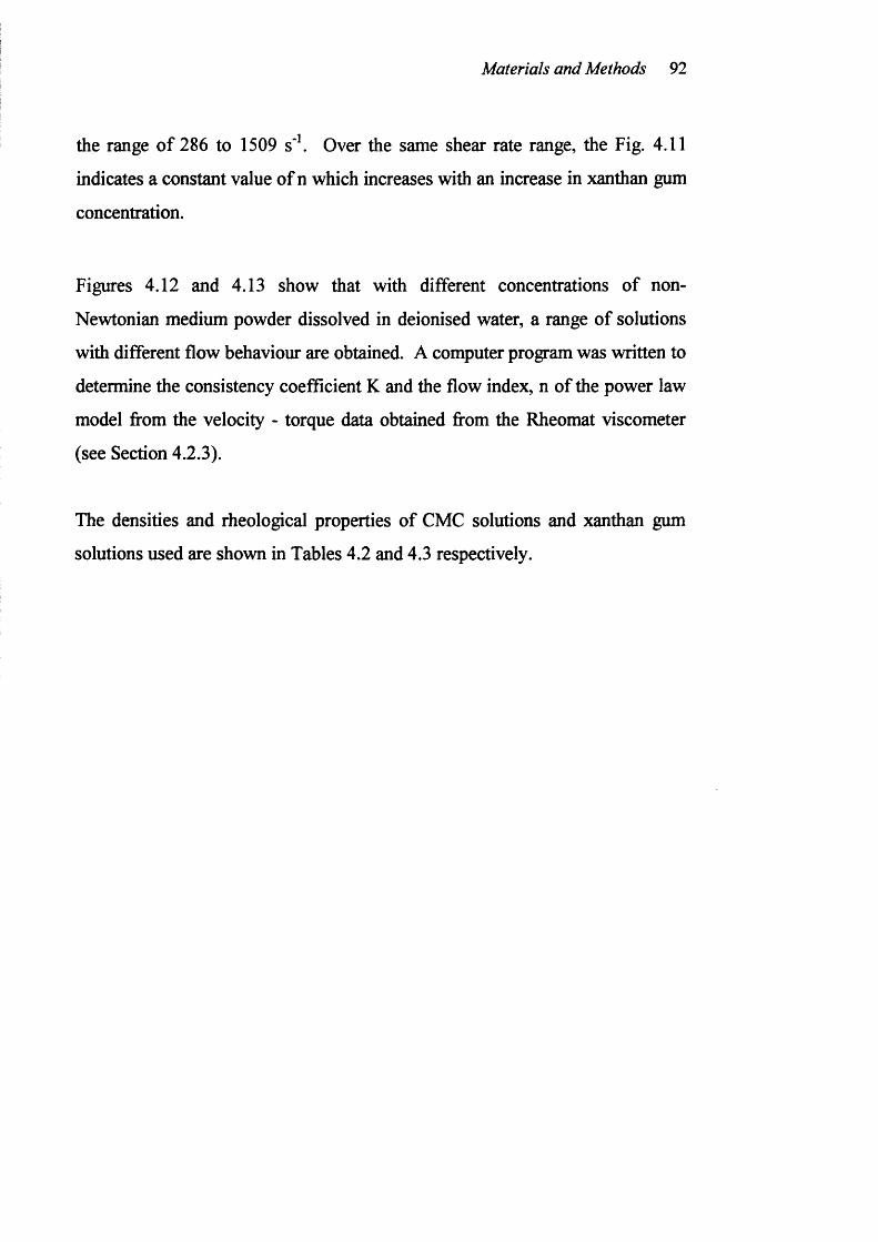
Materials and Methods 92
the range o f 286 to 1509 s"\ Over the same shear rate range, the Fig. 4.11
indicates a constant value of n which increases with an increase in xanthan gum
concentration.
Figures 4.12 and 4.13 show that with different concentrations of non-
Newtonian medium powder dissolved in deionised water, a range of solutions
with different flow behaviour are obtained. A computer program was written to
determine the consistency coefficient K and the flow index, n of the power law
model fi’om the velocity - torque data obtained fi*om the Rheomat viscometer
(see Section 4.2.3).
The densities and rheological properties o f CMC solutions and xanthan gum
solutions used are shown in Tables 4.2 and 4.3 respectively.
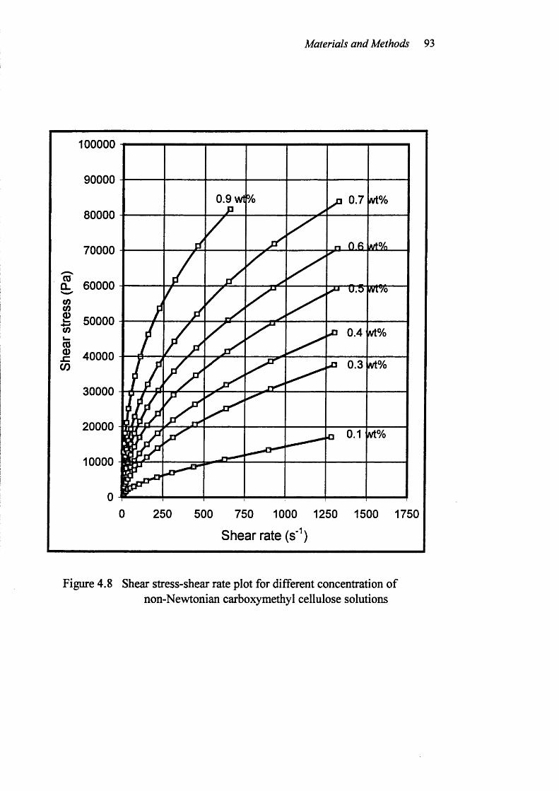
Materials and Methods 93
100000
90000
0.9 wt%80000
70000
S . 60000CO(p_ 50000CO
COQ).c 400000.3 m oCO
30000
200000.1 m o
10000
0 250 500 750 1000 1250 1500 1750
Shear rate (s‘ )
Figure 4.8 Shear stress-shear rate plot for different concentration ofnon-Newtonian carboxymethyl cellulose solutions
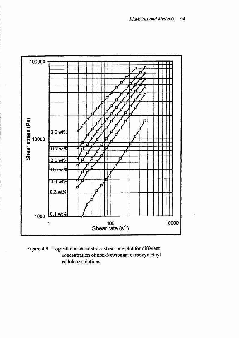
Materials and Methods 94
100000 1
0.9 wt%10000
0.4 wt°/o
1000 wt°410000100 .
Shear rate (s )
Figure 4.9 Logarithmic shear stress-shear rate plot for differentconcentration of non-Newtonian carboxymethylcellulose solutions
Materials and Methods 95
50000
0.9 wt%45000
40000
35000
30000 0.7 wt%
250000.5 wt% 0.4 wt%200000.3 wt%
15000
0.1 wt%10000
5000
400 800 1200 Shear rate (s' )
1600 2000
Figure 4.10 Shear stress-shear rate plot for different concentrationof non-Newtonian xanthan gum solutions
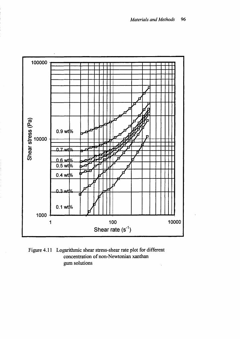
Materials and Methods 96
100000
0.9 wt£ 10000
0.7 wt
0.6 wt 0.5 wt
0.4 wt
0.1 wt
1000 J10000100
Shear rate (s' )
Figure 4.11 Logarithmic shear stress-shear rate plot for differentconcentration of non-Newtonian xanthangum solutions
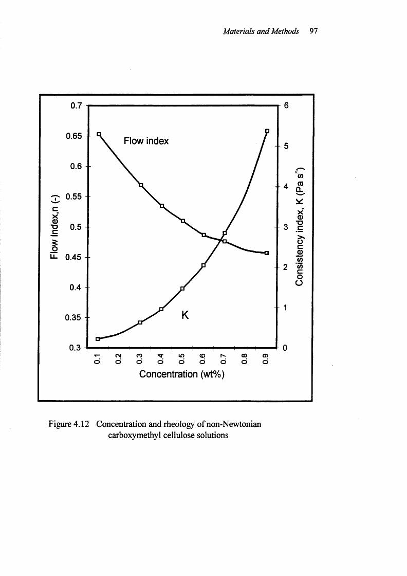
Materials and Methods 97
o
I
0.7
0.65 Flow index
0.6
0.55
0.5
0.45
0.4
0.35
0.3COd
CDdd
COd
G)d
CNdo
- 5
-- 4
0
Concentration (wt%)
CO
(0Û.
0)■ Dc
ICOcoo
Figure 4.12 Concentration and rheology of non-Newtonian carboxymethyl cellulose solutions
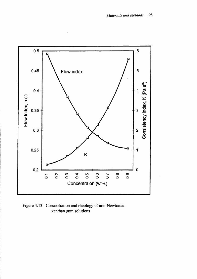
Materials and Methods 98
0.5
0.45 Flow index
-- 40.4I
c
■o 0.35Ç
ILi.
0.3 -
0.25
0.2 4O)d
COd
I D
dCD
dood
CNJ
d do
CO
COÛ.
0)"OÇ
ICOcoO
Concentralon (wt%)
Figure 4.13 Concentration and rheology of non-Newtonian xanthan gum solutions
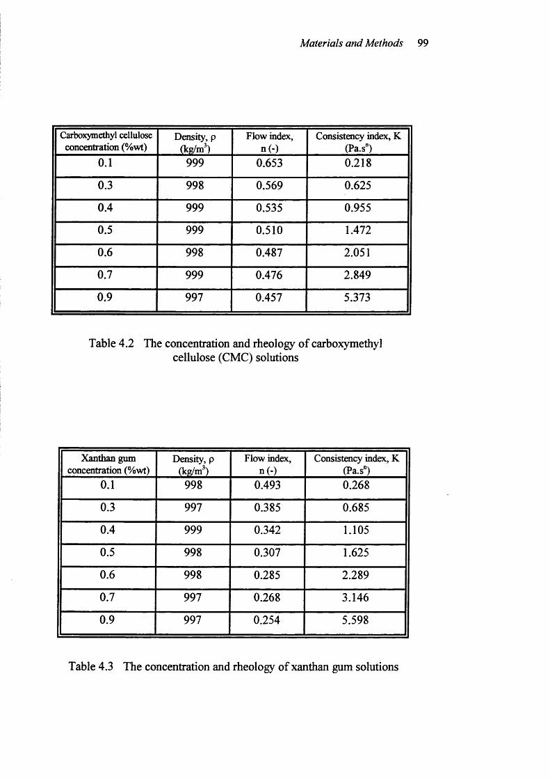
Materials and Methods 99
Carboxymethyl cellulose concentration (%wt)
Density, p (kg/m )
Flow index, n(-)
Consistency index, K (Pa.s")
0.1 999 0.653 0.218
0.3 998 0.569 0.625
0.4 999 0.535 0.955
0.5 999 0.510 1.472
0.6 998 0.487 2.051
0.7 999 0.476 2.849
0.9 997 0.457 5.373
Table 4.2 The concentration and rheology of carboxymethyl cellulose (CMC) solutions
Xanthan gum concentration (%wt)
Density, p (kg/m )
Flow index, n(-)
Consistency index, K (Pa.s")
0.1 998 0.493 0.268
0.3 997 0.385 0.685
0.4 999 0.342 1.105
0.5 998 0.307 1.625
0.6 998 0.285 2.289
0.7 997 0.268 3.146
0.9 997 0.254 5.598
Table 4.3 The concentration and rheology of xanthan gum solutions
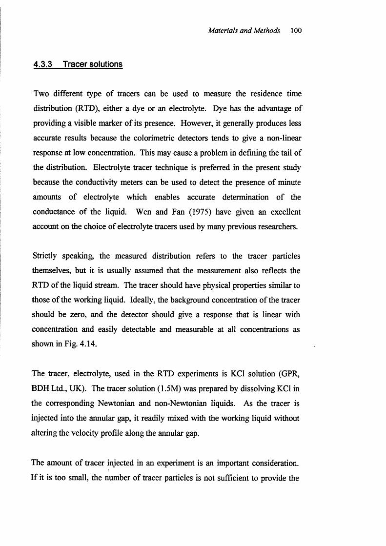
Materials and Methods 100
4.3.3 Tracer solutions
Two different type of tracers can be used to measure the residence time
distribution (RTD), either a dye or an electrolyte. Dye has the advantage of
providing a visible marker o f its presence. However, it generally produces less
accurate results because the colorimetric detectors tends to give a non-linear
response at low concentration. This may cause a problem in defining the tail of
the distribution. Electrolyte tracer technique is preferred in the present study
because the conductivity meters can be used to detect the presence of minute
amounts o f electrolyte which enables accurate determination of the
conductance o f the liquid. Wen and Fan (1975) have given an excellent
account on the choice o f electrolyte tracers used by many previous researchers.
Strictly speaking, the measured distribution refers to the tracer particles
themselves, but it is usually assumed that the measurement also reflects the
RTD of the liquid stream. The tracer should have physical properties similar to
those of the working liquid. Ideally, the background concentration of the tracer
should be zero, and the detector should give a response that is linear with
concentration and easily detectable and measurable at all concentrations as
shown in Fig. 4.14.
The tracer, electrolyte, used in the RTD experiments is KCl solution (GPR,
BDH Ltd., UK). The tracer solution (1.5M) was prepared by dissolving KCl in
the corresponding Newtonian and non-Newtonian liquids. As the tracer is
injected into the annular gap, it readily mixed with the working liquid without
altering the velocity profile along the annular gap.
The amount of tracer injected in an experiment is an important consideration.
If it is too small, the number of tracer particles is not sufficient to provide the
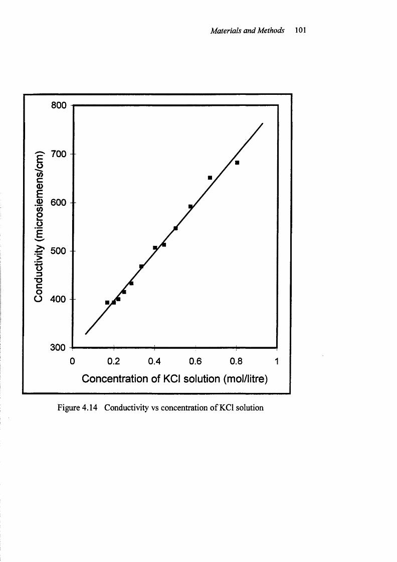
Materials and Methods 101
800
700 -
600 --
500 -
"O
400 --
3000.2
Concentration of KOI solution (mol/litre)
0.4 0.80.6
Figure 4.14 Conductivity vs concentration o f KCl solution
Materials and Methods 102
16 1
14 -□ A
ooco
Tracerweight
2 o 3 ml A 2.5 ml o 2 ml □ 1.5 ml
1c8
CO
$coCOc0)Eb
1 AO O
0.8 0.9 1 1.2 1.31.1
Dimensionless time, 0 (-)
Figure 4.15 The influence of the amount of tracer injected on the dimensionless RTD
Materials and Methods 103
desired accuracy for analysis. If it is too large, it may generate "pseudo" flow
which can seriously distort the true flow pattern. The effect o f the amount of
tracer used on the dimensionless residence time distribution is shown in Fig.
4.15, which gives results for injected impulse o f 1.5, 2, 2.5 and 3.0 ml. It is
evident that the dimensionless outlet tracer concentration was not affected
significantly by the amount of tracer injected. Based on this result, 1.5 ml o f
tracer would be used in all experiments.
4.4 Methods
4.4.1 Experimental procedures
In every experiments, steady-state flow conditions were assured prior to the
introduction of the tracer by running liquid medium through the annular gap
until the discharge flow rate remained steady for several sampling intervals.
The conductivity probes were inserted in the measuring stations and were
connected to the conductivity meters. The electrolytic tracer was rapidly
injected manually with a hypodermic syringe and the recording of tracer
concentrations at the two stations were initiated automatically and
simultaneously. In all cases the injected volume was less than one-thousandth
of the volume o f the liquid in the gap. Therefore, the effect of the tracer upon
the flow pattern was ignored. Moreover, it was assumed that the tracer
particles was injected over a sufficient small time interval (approximately one
second) that the idealisation of an instantaneous pulse (impulse) stimulus was
suitable.
With the liquid flowing through the annular gap, conductivity probes then
detected the tracer as it passed by the electrodes. The change of the
conductivity with time was recorded at each station using the data acquisition
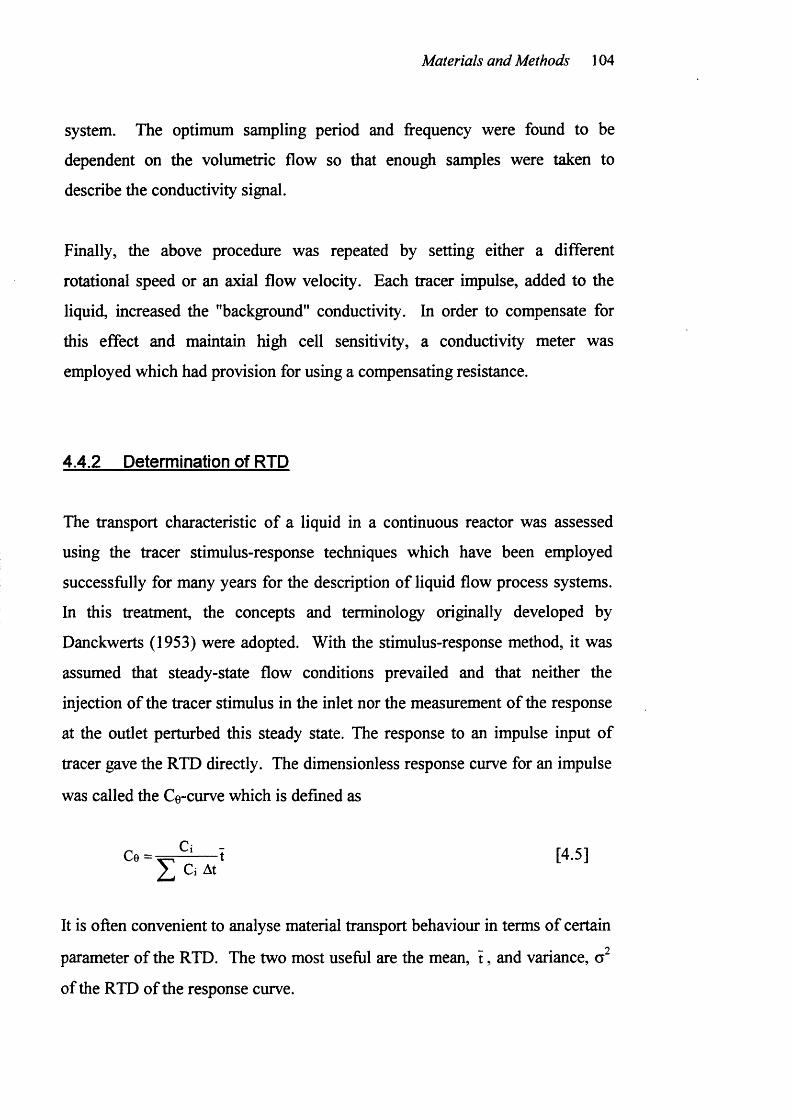
Materials and Methods 104
system. The optimum sampling period and frequency were found to be
dependent on the volumetric flow so that enough samples were taken to
describe the conductivity signal.
Finally, the above procedure was repeated by setting either a different
rotational speed or an axial flow velocity. Each tracer impulse, added to the
liquid, increased the "background" conductivity. In order to compensate for
this effect and maintain high cell sensitivity, a conductivity meter was
employed which had provision for using a compensating resistance.
4.4.2 Determination of RTD
The transport characteristic o f a liquid in a continuous reactor was assessed
using the tracer stimulus-response techniques which have been employed
successfully for many years for the description of liquid flow process systems.
In this treatment, the concepts and terminology originally developed by
Danckwerts (1953) were adopted. With the stimulus-response method, it was
assumed that steady-state flow conditions prevailed and that neither the
injection of the tracer stimulus in the inlet nor the measurement of the response
at the outlet perturbed this steady state. The response to an impulse input of
tracer gave the RTD directly. The dimensionless response curve for an impulse
was called the Ce-curve which is defined as
= ^ - - t [4.5]S Ci At
It is often convenient to analyse material transport behaviour in terms of certain
parameter of the RTD. The two most useful are the mean, t , and variance,
of the RTD of the response curve.
Materials and Methods 105
Z t C A t
t = [4.6]Ê C At
00.2Z r c At
------------- 1" [4.7]Z C At0
4.4.3 Data acquisition system
The electrical conductivity signal produced by the conductivity meters and the
rotational speed deduced by the speed/torque transducer with respect to time
are measured in the present study. These measurements were directed into the
data acquisition system shown in Fig. 4.16. This essentially consisted o f a
measurement and control device for data storage and processing (Keithley
Model 575 measurement and control system, KDAC 500/1 data acquisition and
control software) and a computer with a BASICA program (see Appendix 4).
The signals from conductivity meters and transducer were converted into digital
signals via an analogue/digital converter which was connected to a clock
generator allowing the operator to monitor the frequency of the samples
recorded. The sampling frequency could be adjusted by a variable dial,
attached to the analogue/digital clock, from 0 - 1,000 samples per second. The
sampling period was set via the main menu of the computer data acquisition
program. The optimum sampling period and frequency were determined by
preliminary trial experiments such that enough samples are taken with
sufficient frequency to completely describe a given fluctuating conductivity
signal. The BASICA programs enabled the operator to (a) instantaneously
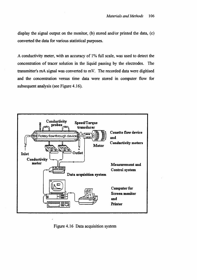
Materials and Methods 106
display the signal output on the monitor, (b) stored and/or printed the data, (c)
converted the data for various statistical purposes.
A conductivity meter, with an accuracy of 1% full scale, was used to detect the
concentration o f tracer solution in the liquid passing by the electrodes. The
transmitter's mA signal was converted to mV. The recorded data were digitised
and the concentration versus time data were stored in computer flow for
subsequent analysis (see Figure 4.16).
Speed/Torque transducer
Rotary flow-through device||^^J^^9
Motor
Outlet
Couette flow device andConductivity meters
Conductivitymeter III Measurement and
Control systemData acquisition system
Computer for Screen monitor and Printer
Figure 4.16 Data acquisition system
Theoretical Results and Discussion 107
CHAPTER FIVE
THEORETICAL RESULTS AND DISCUSSION
5.1 Introduction
The purpose o f this chapter is to present the theoretical results o f the eigenvalue
problems which govern various modes o f flow instability of the steady Couette
flow subject to perturbations o f the form of Taylor vortices. Consideration is
given to the cases o f both Newtonian and non-Newtonian liquids.
In Section 5.2, a numerical solution to the classical flow stability o f pure
Couette flow, in which the axial Reynolds number equals to zero, is briefly
discussed. The results will be compared with the previous works in order to
assess the validity o f the present numerical method derived in Chapter 3.
Engineers often encounter the axial flow in the annulus between the rotating
cylinders. When the forced axial flow is superimposed on the Couette flow,
the stability o f liquid motion will be affected. In Section 5.3, the problem o f
flow instability o f such a flow is discussed.
The instability o f the Couette flow is also critically affected by rheological
properties o f the non-Newtonian liquids. In Section 5.4 the dependence o f the
stability limit on shear thinning behaviour of non-Newtonian material is
investigated theoretically for the case of purely viscous liquid with the power
law viscosity and the wide gap geometry.
All the theoretical results shown in this chapter were obtained by using the
Galerkin method (Appendix 1) for both Newtonian and non-Newtonian liquids
respectively. Computations were carried out by using the Mathematica
software which are presented in Appendix 2 and 3 respectively.
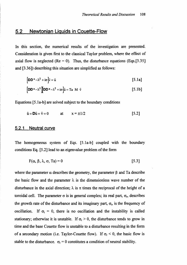
Theoretical Results and Discussion 108
5.2 Newtonian Liquids in Couette-Flow
In this section, the numerical results of the investigation are presented.
Consideration is given first to the classical Taylor problem, where the effect of
axial flow is neglected (Re = 0). Thus, the disturbance equations (Eqs.[3.35]
and [3.36]) describing this situation are simplified as follows:
[DD*-X^+ic]v = û [5.1a]
[DD*-X^|DD*-A.2+ia]û = Ta M v [5.1b]
Equations [5.1a-b] are solved subject to the boundary conditions
û = Dû = v = 0 at X = ±1/2 [5.2]
5.2.1 Neutral curve
The homogeneous system o f Eqs. [5.1a-b] coupled with the boundary
conditions Eq. [5.2] lead to an eigenvalue problem of the form
F(a, P, 1, a. Ta) = 0 [5.3]
where the parameter a describes the geometry, the parameter p and Ta describe
the basic flow and the parameter X is the dimensionless wave number of the
disturbance in the axial direction; A, is 7i times the reciprocal of the height o f a
toroidal cell. The parameter a is in general complex; its real part, Gr» describes
the growth rate o f the disturbance and its imaginary part, Ci, is the frequency of
oscillation. If O i - 0, there is no oscillation and the instability is called
stationary; otherwise it is unstable. If Gr > 0, the disturbance tends to grow in
time and the base Couette flow is unstable to a disturbance resulting in the form
of a secondary motion (i.e. Taylor-Couette flow). If Gr < 0, the basic flow is
stable to the disturbance. Gr = 0 constitutes a condition of neutral stability.
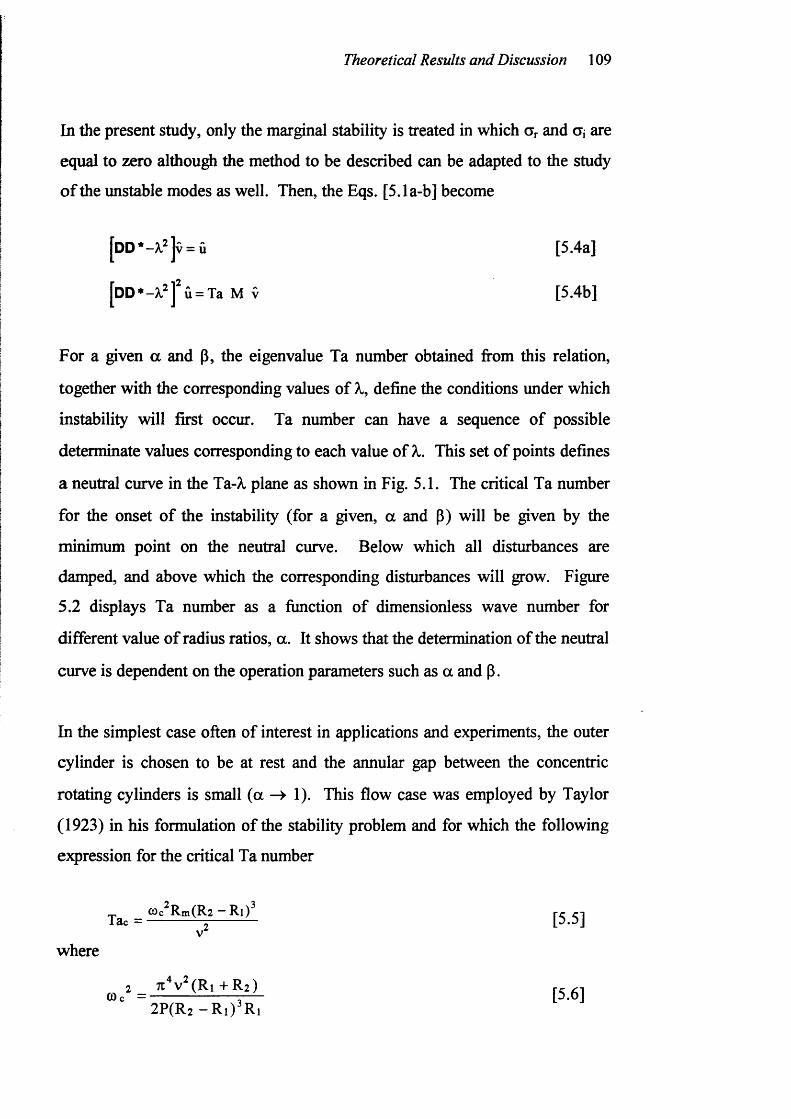
Theoretical Results and Discussion 109
In the present study, only the marginal stability is treated in which Gr and G{ are
equal to zero although the method to be described can be adapted to the study
o f the unstable modes as well. Then, the Eqs. [5.1a-b] become
[dD*-A, ]v = û [5.4a]
[DD*-X, ]^û = Ta M V [5.4b]
For a given a and P, the eigenvalue Ta number obtained from this relation,
together with the corresponding values of X,, define the conditions under which
instability will first occur. Ta number can have a sequence of possible
determinate values corresponding to each value of X. This set o f points defines
a neutral curve in the Ta-X plane as shown in Fig. 5.1. The critical Ta number
for the onset o f the instability (for a given, a and P) will be given by the
minimum point on the neutral curve. Below which all disturbances are
damped, and above which the corresponding disturbances will grow. Figure
5.2 displays Ta number as a fimction of dimensionless wave number for
different value o f radius ratios, a. It shows that the determination of the neutral
curve is dependent on the operation parameters such as a and p.
In the simplest case often of interest in applications and experiments, the outer
cylinder is chosen to be at rest and the annular gap between the concentric
rotating cylinders is small (a -> 1). This flow case was employed by Taylor
(1923) in his formulation of the stability problem and for which the following
expression for the critical Ta number
where
[5.5]V
nV(Ri + R,) [5.6]2P(R2 - R i ) ' R ]
Theoretical Results and Discussion 110
3300
3100
2900
2700 - Neutral curve, a = 0
f 2500 -
Unstablec 2300 -
(0I - 2100
Stable1900 -
Critical Taylor num ber, Tac
1700
Crrtical dim ensionless 'wave num ber, 7
1500 J
Dimensionless wave number, X (-)
Figure 5.1 Typical neutral curve in the Ta - 1 plane
Theoretical Results and Discussion 111
2150a = 0.9
2100 a = 0.925
a = 0.952050
a = 0.9752000
a = 0.99
1950
1900 -
1850
1800
1750
1700
1650
Dimensionless wave number, X (-)
Figure 5.2 Neutral curve in the Ta-X plane at different radius ratios
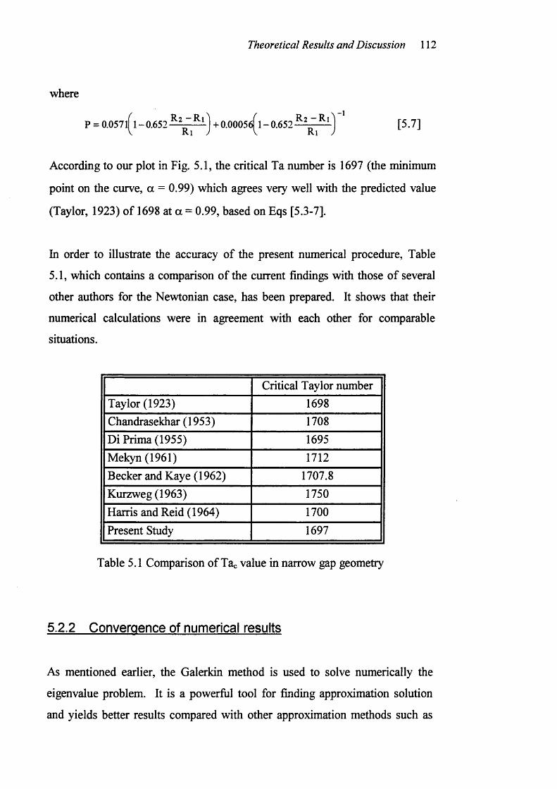
Theoretical Results and Discussion 112
where
P = 0.057l( l - 0.652 — + 0.00056( 1 - 0.652-1
[5.7]
According to our plot in Fig. 5.1, the critical Ta number is 1697 (the minimum
point on the curve, a = 0.99) which agrees very well with the predicted value
(Taylor, 1923) o f 1698 at a = 0.99, based on Eqs [5.3-7].
In order to illustrate the accuracy of the present numerical procedure. Table
5.1, which contains a comparison of the current findings with those of several
other authors for the Newtonian case, has been prepared. It shows that their
numerical calculations were in agreement with each other for comparable
situations.
Critical Taylor numberTaylor (1923) 1698Chandrasekhar (1953) 1708Di Prima (1955) 1695Mekyn (1961) 1712Becker and Kaye (1962) 1707.8Kurzweg (1963) 1750Harris and Reid (1964) 1700Present Study 1697
Table 5.1 Comparison of Tac value in narrow gap geometry
5.2.2 Convergence of numerical results
As mentioned earlier, the Galerkin method is used to solve numerically the
eigenvalue problem. It is a powerful tool for finding approximation solution
and yields better results compared with other approximation methods such as
Theoretical Results and Discussion 113
method o f moment, collocation method, subdomain method and least square
method. The theory of this method is given Appendix 1. Basically, this
method consists of expansion of û and v from Eq. [5.4a-b] in complete sets o f
series functions (trial function) satisfying the boundary conditions. The
coefficients in the trial function are determined by the requirement that the
residual function be orthogonal to the expansion functions for û and v
respectively. This leads to a system o f infinitely many linear, homogeneous
equations for the coefficients in the series. For a non-trivial solution it is
necessary that the determinant o f the system o f equations vanish, and this gives
a determinant equation for Taylor number. The convergence of the numerical
results can always be improved by increasing the number of (N) functions used.
In practice only a finite number of terms are used in the series for û and v , say
N, and this leads to a determinant of size 2N. The evaluation of the
determinant programmed in the Mathematica software (Appendix 2 and 3).
For the present study, computations have been performed for increasing values
o fN until two successive values o f Taylor number are found that differ by less
than 1% (usually N = 3 or 4) as shown in Fig. 5.3. The instability problem
were carried out for a range of values o f radius ratio, a. For a = 0.995, and p =
0 the results for N = 4 are within 0.2% of the "the exact results" given by
Chandrasekhar (1961). Indeed even with N = 2, the error is within 5%. If we
bear in mind that the analytical and numerical work using the Galerkin method
with N = 2 is much less than that for the expansion procedure o f Chandrasekhar
(1961). For a = 0.5 and N = 4 the maximum difference between the present
results and those of Chandrasekhar and Elbert (1963) occurs at a = 0.5 is about
2%. With decreasing a (wider-gap geometry) it becomes more difficult to
approximate the eigenfunction, so that a < 0.2 it was not possible to determine
Ta number accurately without taking more terms in the series for û and v . By
comparing the results for N = 2, 3 and 4 it is estimated that all the results given
for N = 4 are generally correct within 2%.
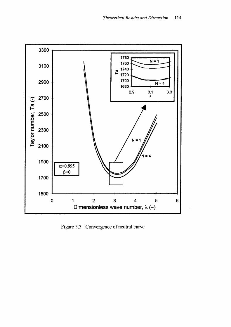
Theoretical Results and Discussion 114
3300
3100
2900
3 2700
fe 2500JQIc 2300L _
o>%CDK 2100
1900
1700
1500
a=0.995(3=0
1780 1N = 1
N = 4
1 2 3 4 5Dimensionless wave number, X (-)
3.3
Figure 5.3 Convergence of neutral curve
Theoretical Results and Discussion 115
5.2.3 The effect of radius ratio on the critical Tavlor number
Figure 5.4 shows the effect of radius ratio on the onset o f flow instability,
expressed as critical Taylor number, Ta , in Couette flow at angular speed ratio,
P = 0. The values o f Tac were obtained from the neutral curves o f Taylor
number - dimensionless wave number plots for different radius ratios. The
figure shows that the critical Ta number can be significantly affected by the
ratio o f the radii o f the two cylinders. It is found that stable state o f the laminar
Couette flow is achieved by having a large gap width (i.e. small radius ratio).
Astill (1964) studied the development o f Taylor vortices between concentric
cylinders with the inner cylinder rotating. He found the flow instability began
as a series o f oscillating waves occurring first near the wall o f the rotating inner
cylinder. In the case o f a wide gap, a high Taylor number is needed for the
vortices to spread to the outer wall. This finding was supported later by Coney
and Simmers (1979) and Pfitzer and Beer (1992).
Figure 5.4 shows that the destabilisation of flow is very sensitive to changes in
a from 0.1 to 0.2. The destabilisation effect of a slows down as a increase
until a equals about 0.5 (i.e. Ri = 0.5 R2). Results from calculations of critical
Ta number for different radius ratios are summarised in Table 5.2 together with
the critical dimensionless wave number. Figure 5.4 also shows the theoretical
results o f Walowit et al. (1964), Sparrow et al (1964) and Roberts et al. (1965)
for comparison with the present results. In general the agreement is excellent.
At the critical Ta number the vortices are characterised by the critical
dimensionless wave number, A,, or in other words, a critical size of the vortices
which is related to the wavelength of a pair o f Taylor vortices. The wavelength
is the most characteristic feature of the Taylor vortices; it can be seen with the
naked eye on the photographs of Taylor vortices by flow visualisation
technique as discussed in Section 2.3.1. Figure 5.5 shows that the value of
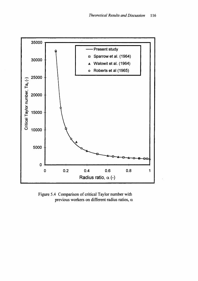
Theoretical Results and Discussion 116
35000
— Present study
□ Sparrow et al. (1964)
A Walowit et al. (1964)
o Roberts et al (1965)
30000 -
25000 -
.Q 20000
15000 -
10000 -
5000 -
0.6 0.80.2 0.4
Radius ratio, a (-)
Figure 5.4 Comparison of critical Taylor number with previous workers on different radius ratios, a
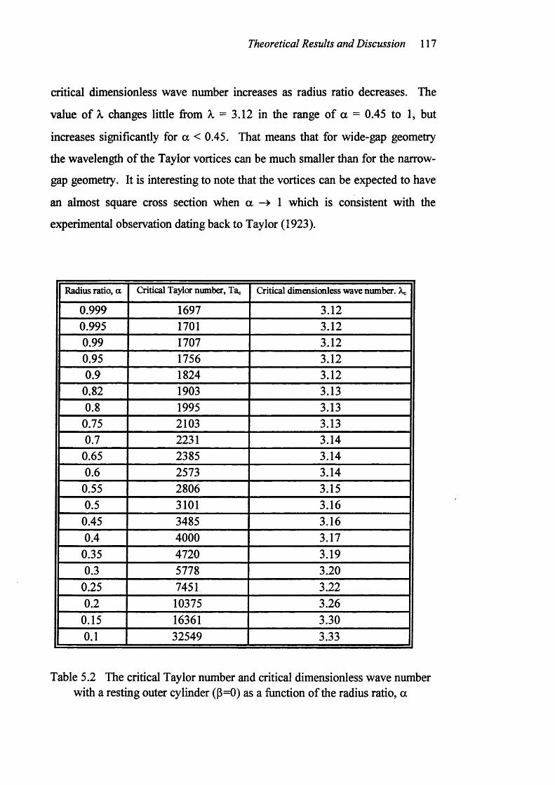
Theoretical Results and Discussion 117
critical dimensionless wave number increases as radius ratio decreases. The
value o f X changes little from ^ = 3.12 in the range o f a = 0.45 to 1, but
increases significantly for a < 0.45. That means that for wide-gap geometry
the wavelength of the Taylor vortices can be much smaller than for the narrow-
gap geometry. It is interesting to note that the vortices can be expected to have
an almost square cross section when a -> 1 which is consistent with the
experimental observation dating back to Taylor (1923).
Radius ratio, a Critical Taylor numb^, Ta« Critical dimoisioaless wave number. A?
0.999 1697 3.120.995 1701 3.120.99 1707 3.120.95 1756 3.120.9 1824 3.12
0.82 1903 3.130.8 1995 3.13
0.75 2103 3.130.7 2231 3.14
0.65 2385 3.140.6 2573 3.14
0.55 2806 3.150.5 3101 3.16
0.45 3485 3.160.4 4000 3.17
0.35 4720 3.190.3 5778 3.20
0.25 7451 3.220.2 10375 3.26
0.15 16361 3.300.1 32549 3.33
Table 5.2 The critical Taylor number and critical dimensionless wave numberwith a resting outer cylinder (p=0) as a function of the radius ratio, a
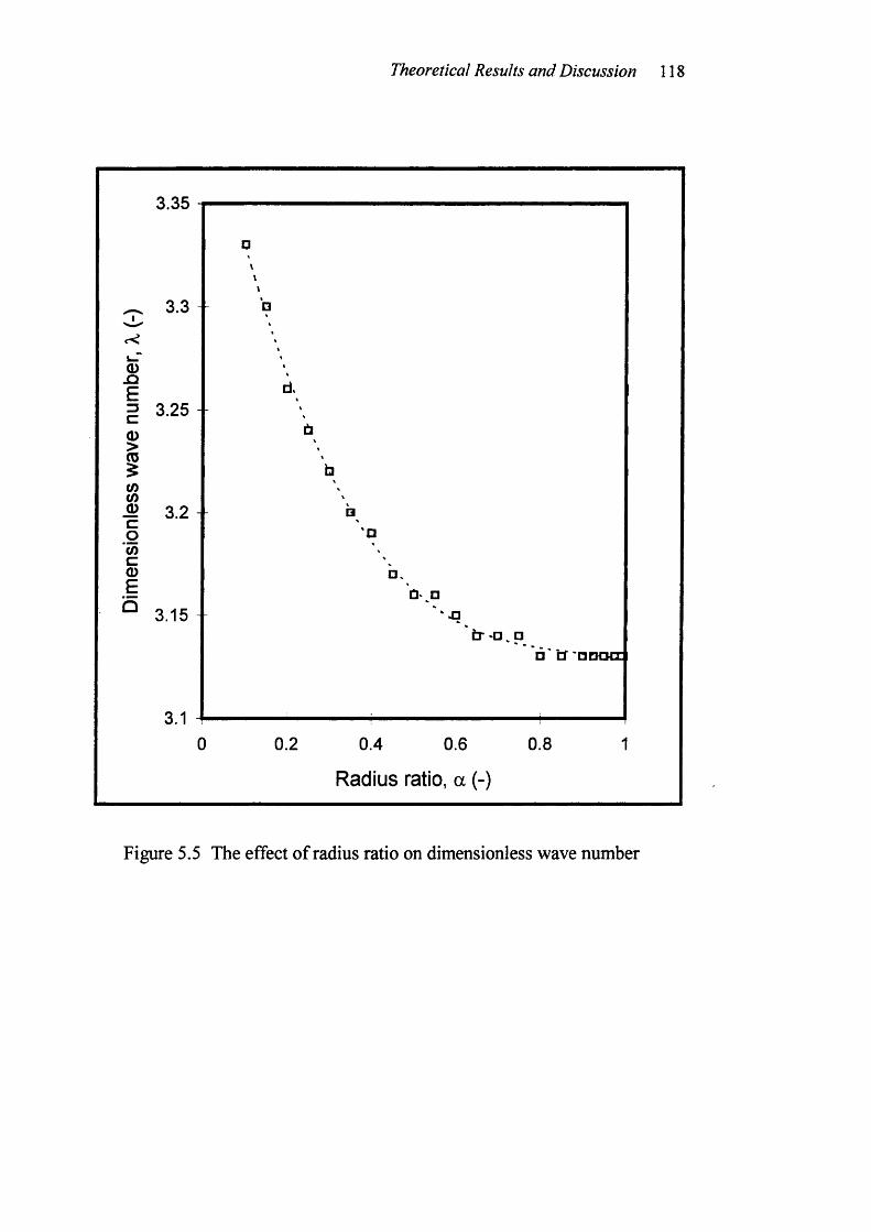
Theoretical Results and Discussion 118
3.35 1
3.3
5Eg 3.25
I(0
^ 3.2 +c oCOc (DE^ 3.15
3.10
d.
Ù □
□ 'd 0 0 0 0 :
0.2 0.4 0.6 0.8
Radius ratio, a (-)
Figure 5.5 The effect of radius ratio on dimensionless wave number
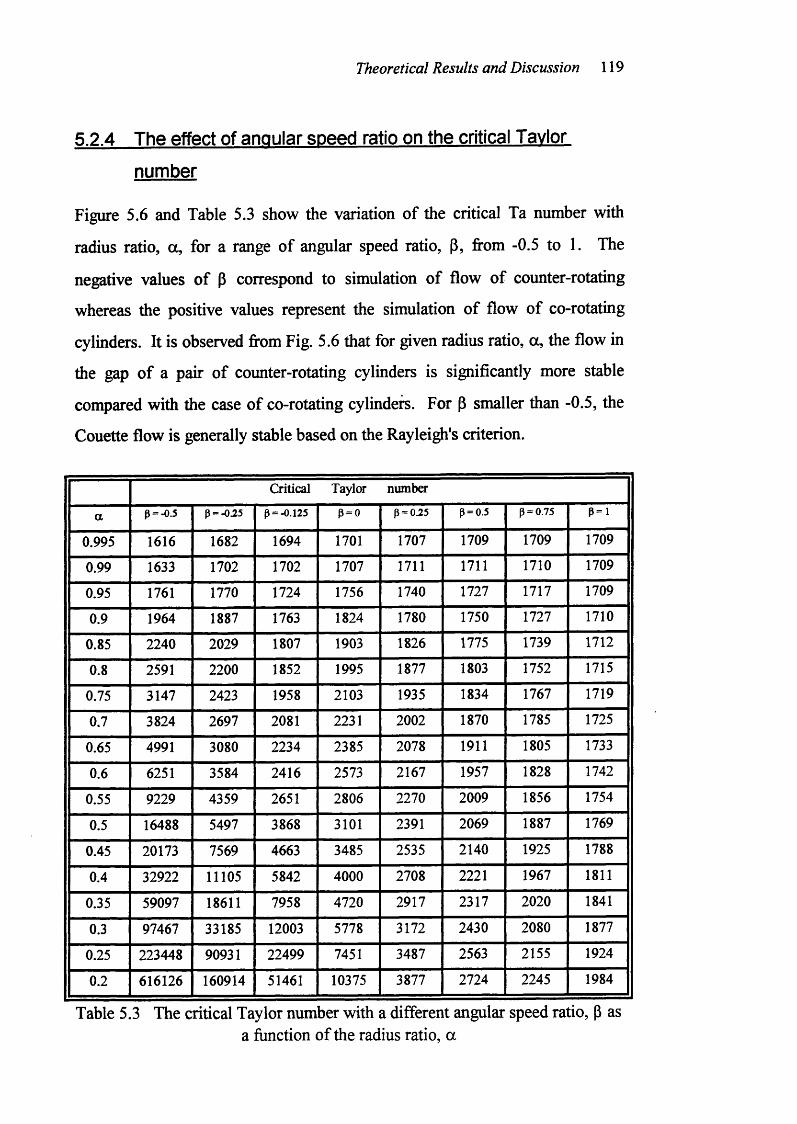
Theoretical Results and Discussion 119
5.2.4 The effect of angular speed ratio on the critical Tavlor
number
Figure 5.6 and Table 5.3 show the variation of the critical Ta number with
radius ratio, a, for a range of angular speed ratio, p, from -0.5 to 1. The
negative values o f P correspond to simulation of flow of counter-rotating
whereas the positive values represent the simulation of flow of co-rotating
cylinders. It is observed from Fig. 5.6 that for given radius ratio, a, the flow in
the gap of a pair o f counter-rotating cylinders is significantly more stable
compared with the case of co-rotating cylinders. For P smaller than -0.5, the
Couette flow is generally stable based on the Rayleigh's criterion.
Critical Taylor number
a p = -0.5 p = -0.25 p = -0.125 3 = 0 3 = 0.25 3 = 0.5 3 = 0.75 3= 1
0.995 1616 1682 1694 1701 1707 1709 1709 1709
0.99 1633 1702 1702 1707 1711 1711 1710 1709
0.95 1761 1770 1724 1756 1740 1727 1717 1709
0.9 1964 1887 1763 1824 1780 1750 1727 1710
0.85 2240 2029 1807 1903 1826 1775 1739 1712
0.8 2591 2200 1852 1995 1877 1803 1752 1715
0.75 3147 2423 1958 2103 1935 1834 1767 1719
0.7 3824 2697 2081 2231 2002 1870 1785 1725
0.65 4991 3080 2234 2385 2078 1911 1805 1733
0.6 6251 3584 2416 2573 2167 1957 1828 1742
0.55 9229 4359 2651 2806 2270 2009 1856 1754
0.5 16488 5497 3868 3101 2391 2069 1887 1769
0.45 20173 7569 4663 3485 2535 2140 1925 1788
0.4 32922 11105 5842 4000 2708 2221 1967 1811
0.35 59097 18611 7958 4720 2917 2317 2020 1841
0.3 97467 33185 12003 5778 3172 2430 2080 1877
0.25 223448 90931 22499 7451 3487 2563 2155 1924
0.2 616126 160914 51461 10375 3877 2724 2245 1984
Table 5.3 The critical Taylor number with a different angular speed ratio, p asa function of the radius ratio, a
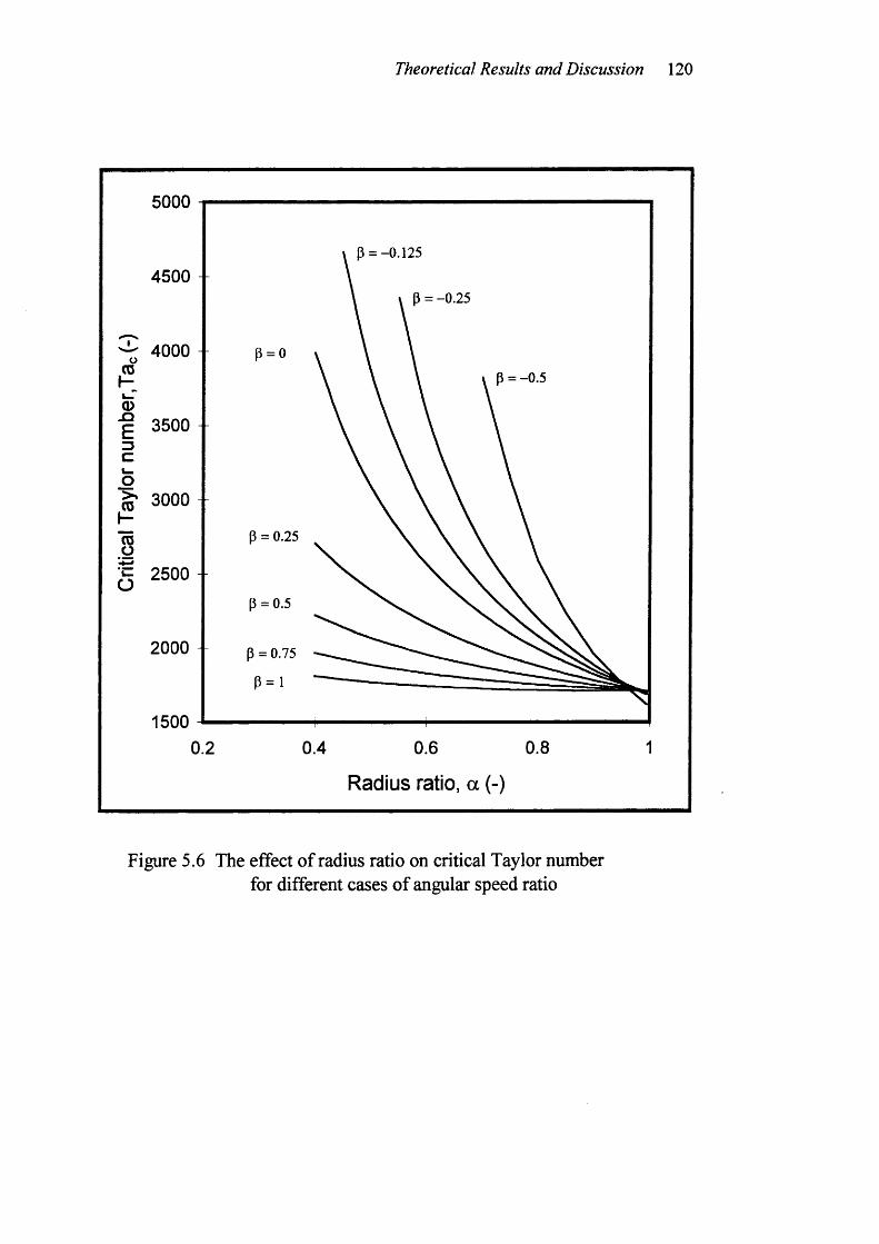
Theoretical Results and Discussion 120
5000 1
P = -0.125
4500P = -0.25
4000 - p = oP = -0.5
c 3500
Sr 3000
P = 0.25
2500 -P = 0.5
2000 - - P = 0.75
1500 J0.80.2 0.4 0.6
Radius ratio, a (-)
Figure 5.6 The effect of radius ratio on critical Taylor number for different cases of angular speed ratio
Theoretical Results and Discussion 121
5.3 Newtonian Liquids in Couette-Flow with Axial Flow
5.3.1 Neutral curve
When an axial flow is superimposed on the Couette flow, the streamlines in the
undisturbed flow become spiral. This complicated combined flow, so-called
Couette-Poiseuille flow, can be characterised as a function o f two independent
parameters: the axial Reynolds number. Re and the Taylor number. Ta. The
system of Eq. [3.31b] and Eq. [3.33] together with boundary conditions Eq.
[3.34] determine an eigenvalue problem of the form
F(a, p, A,, a, Ta, Re) = 0 [5.8]
Analogous with the case o f pure Couette flow, the above parameters are similar
to Eq. [5.3] except for the addition of axial Reynolds number which is defined
by using the mean axial velocity. The condition of the flow stability can be
determined in the form of functional dependence of the critical value of the Ta
number on the Re number, for a given value of a and p.
However, the parameter a is more complicated because for an arbitrarily value
o f a, the Ta number will in general be complex. Thus, unlike the previous
case, the real part of a is no longer assumed to be zero. The motion will be
stable or unstable as the imaginary part o f o is respectively positive or negative.
We shall only consider the neutrally stable case, imaginary part o f a equal to
zero. Mathematically the problem is the following: for given a, p and Re, the
minimum positive real value of Ta number is determined with respect to real
positive values o f X and real values of a. The corresponding values o f X and a
determine the dimensionless wave number and the frequency o f the secondary
motion.
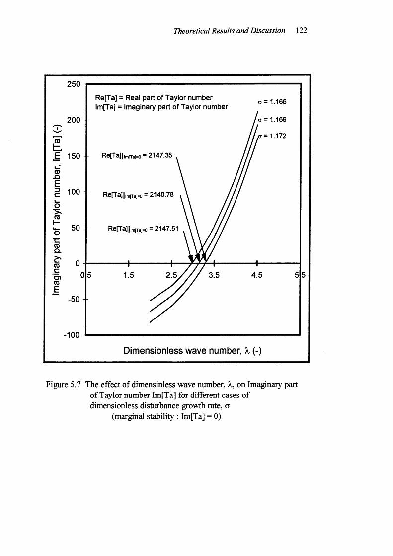
Theoretical Results and Discussion 122
250Re[Ta] = Real part of Taylor number lm[Ta] = Imaginary part of Taylor number
CT = 1.166
200 CT = 1.169
.a = 1.172
E 150 Re[Ta] I im p-a]= o - 2147.35
? 100 Re[Ta]|it7i[Ta]=o - 2140.78
50 - Re[Ta]|imfTa]=o ~ 2147.51
Q.
4.52.5 3.5D)
-50
-100 J
Dimensionless wave number, X (-)
Figure 5.7 The effect of dimensinless wave number, À, on Imaginary part of Taylor number Im[Ta] for different cases of dimensionless disturbance growth rate, a
(marginal stability : lm[Ta] = 0)
Theoretical Results and Discussion 123
It is clear that the determination o f the critical Ta number is a rather
complicated five-parameter problem (Re, cx, P, a and A,). In the iteration
procedure to determine the critical value, calculation is started with available
values of critical Ta number and X found from previous section with a = 0 for
Re = 0. Iterations continue for increasing Re number. For Ta number,
minimum positive determinant is obtained by iteration of a pair (a, X ) as shown
in 5.7. Simulations of the critical Ta number were found to be more sensitive
to changes in the value of a compared with X for given a and p. Completion of
the process just described yields a single point on a neutral stability curve.
Therefore, in searching for the critical Ta number, the increment Aa was kept
as small as possible in order to find the minimum positive real Ta number,
which in turn was minimised over all real positive X as shown in Fig. 5.7.
5.3.2 The effect of axial Reynolds number on the
critical Tavlor number
Figure 5.8 shows the results o f the present study o f critical Ta number versus
Re number plotted with the results of other investigations for a = 0.95 and P =
0. It shows that these simulations compare well with results published by
previous researchers for the case o f narrow gaps. They generally show that the
value of the critical Ta number increases as the Re number increases. Thus, the
axial Re number has an effect in delaying criticality and damping of the initial
formation of Taylor vortices in annuli. In other words, increased stability of
the laminar flow in the annuli can be achieved by imposing an axial flow.
Coney and Simmers (1979) and Abdallah and Coney (1988) experimentally
showed that the axial flow practically confined the vortices to a restricted
region of the annular gap until the rotational speed had increased sufficiently to
enable the vortices to extend to the outer wall. The variation of the critical Ta
number with Re number for a = 0.95 and p = 0 with associated eigenvalue o f X
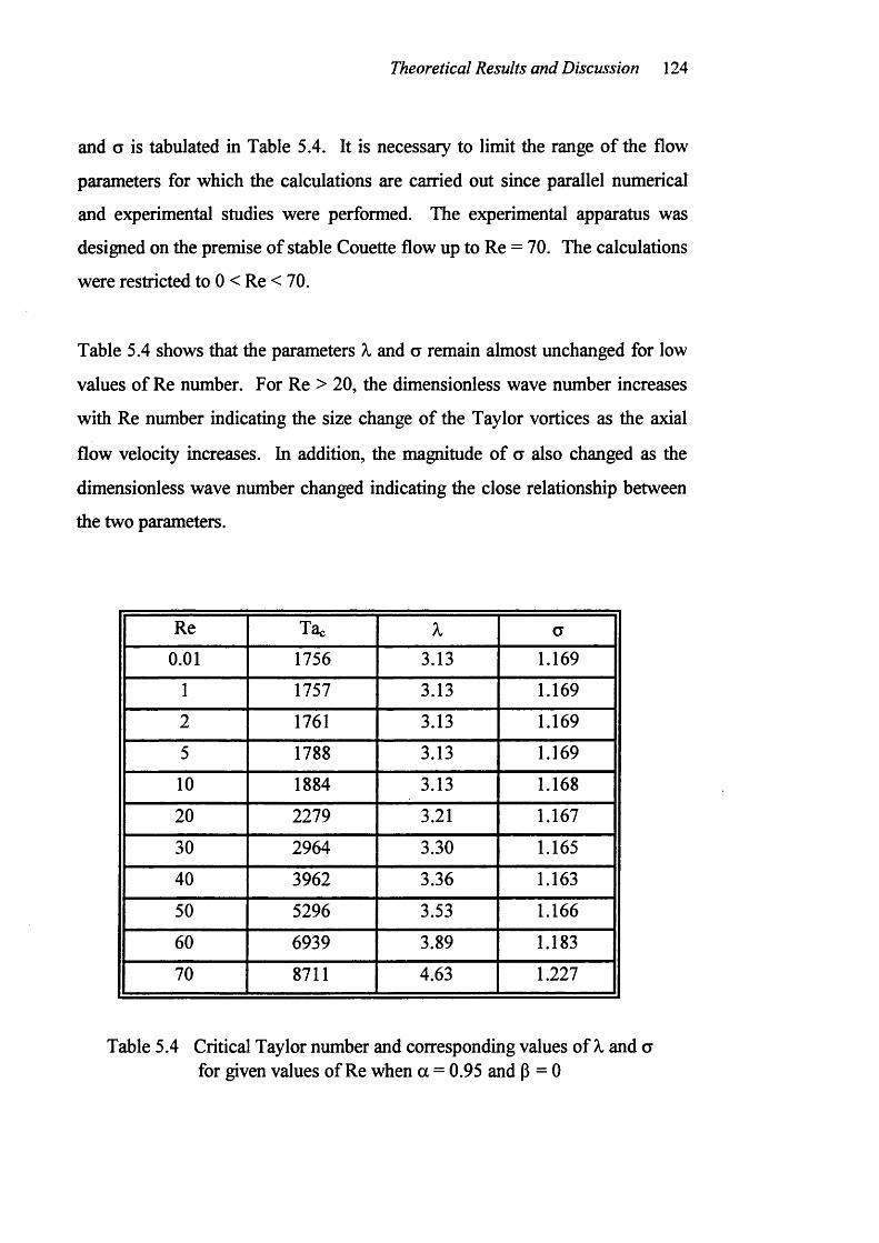
Theoretical Results and Discussion 124
and a is tabulated in Table 5.4. It is necessary to limit the range of the flow
parameters for which the calculations are carried out since parallel numerical
and experimental studies were performed. The experimental apparatus was
designed on the premise of stable Couette flow up to Re = 70. The calculations
were restricted to 0 < Re < 70.
Table 5.4 shows that the parameters X and ct remain almost unchanged for low
values o f Re number. For Re > 20, the dimensionless wave number increases
with Re number indicating the size change of the Taylor vortices as the axial
flow velocity increases. In addition, the magnitude o f g also changed as the
dimensionless wave number changed indicating the close relationship between
the two parameters.
Re Tac X a0.01 1756 3.13 1.169
1 1757 3.13 1.169
2 1761 3.13 1.169
5 1788 3.13 1.169
10 1884 3.13 1.168
20 2279 3.21 1.167
30 2964 3.30 1.165
40 3962 3.36 1.163
50 5296 3.53 1.166
60 6939 3.89 1.183
70 8711 4.63 1.227
Table 5.4 Critical Taylor number and corresponding values of X and a for given values of Re when a = 0.95 and (3 = 0
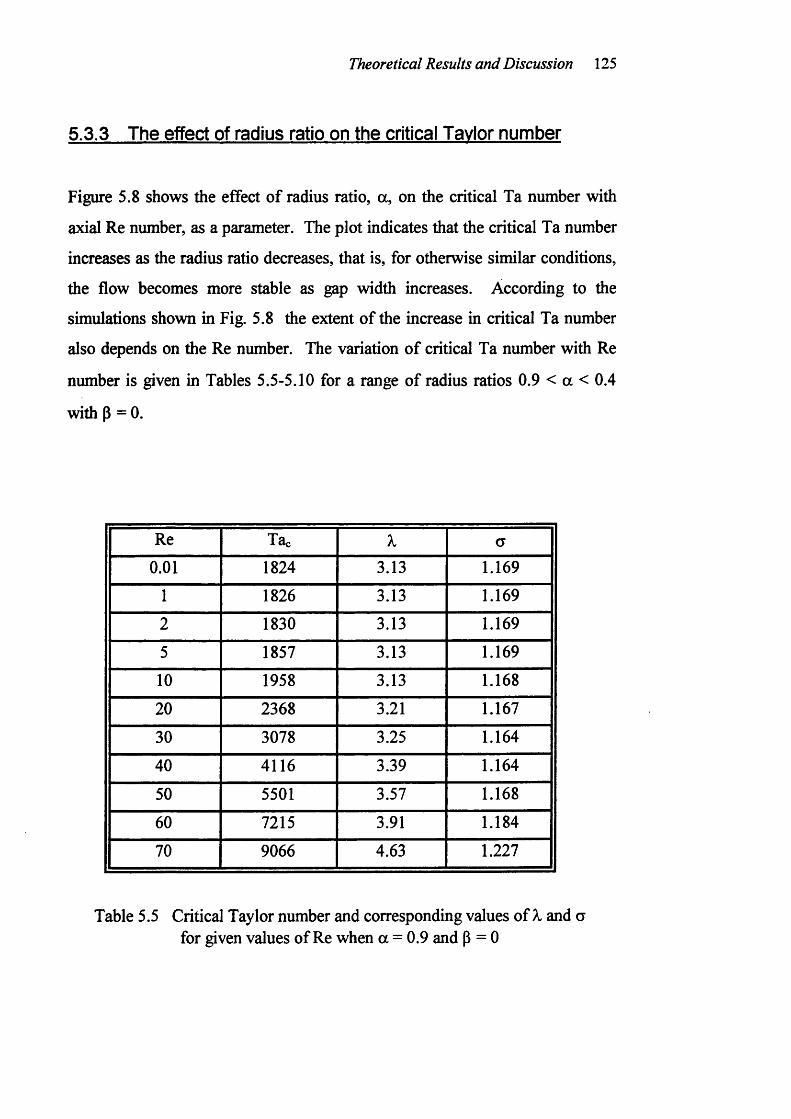
Theoretical Results and Discussion 125
5.3.3 The effect of radius ratio on the critical Tavlor number
Figure 5.8 shows the effect o f radius ratio, a, on the critical Ta number with
axial Re number, as a parameter. The plot indicates that the critical Ta number
increases as the radius ratio decreases, that is, for otherwise similar conditions,
the flow becomes more stable as gap width increases. According to the
simulations shown in Fig. 5.8 the extent of the increase in critical Ta number
also depends on the Re number. The variation o f critical Ta number with Re
number is given in Tables 5.5-5.10 for a range of radius ratios 0.9 < a < 0.4
with P = 0.
Re Tac X G
0.01 1824 3.13 1.169
1 1826 3.13 1.169
2 1830 3.13 1.169
5 1857 3.13 1.169
10 1958 3.13 1.168
20 2368 3.21 1.167
30 3078 3.25 1.164
40 4116 3.39 1.164
50 5501 3.57 1.168
60 7215 3.91 1.184
70 9066 4.63 1.227
Table 5.5 Critical Taylor number and corresponding values of X and a for given values of Re when a = 0.9 and p = 0
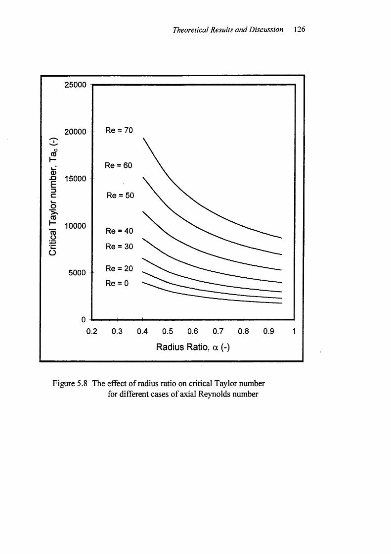
Theoretical Results and Discussion 126
25000
20000 - Re = 70
Re = 60
■9 15000
Re = 50
10000 - - Re = 40
Re = 30
Re = 205000 -Re = 0
0.2 0.3 0.4 0.5 0.6 0.7 0.8 0.9
Radius Ratio, a (-)
Figure 5.8 The effect of radius ratio on critical Taylor number for different cases of axial Reynolds number
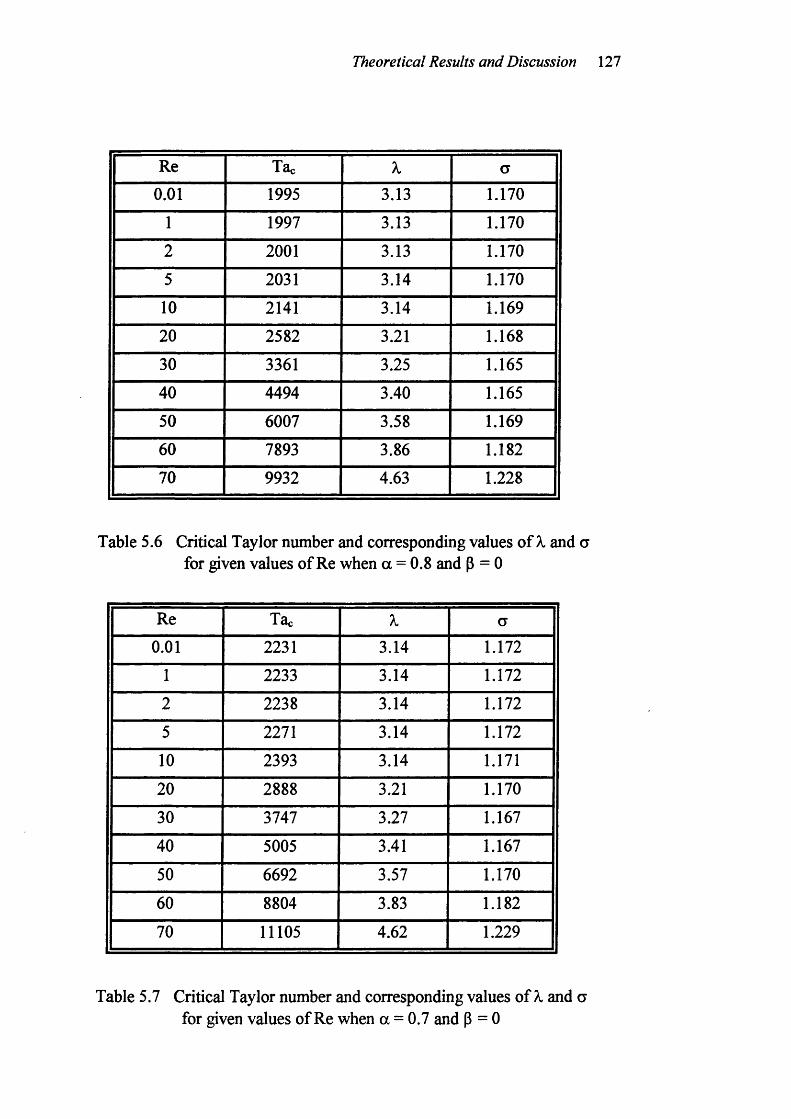
Theoretical Results and Discussion 127
Re Tac X a0.01 1995 3.13 1.170
1 1997 3.13 1.170
2 2001 3.13 1.170
5 2031 3.14 1.170
10 2141 3.14 1.169
20 2582 3.21 1.168
30 3361 3.25 1.165
40 4494 3.40 1.165
50 6007 3.58 1.169
60 7893 3.86 1.182
70 9932 4.63 1.228
Table 5.6 Critical Taylor number and corresponding values o f X and a for given values of Re when a = 0.8 and p = 0
Re Tac X a0.01 2231 3.14 1.172
1 2233 3.14 1.172
2 2238 3.14 1.172
5 2271 3.14 1.172
10 2393 3.14 1.171
20 2888 3.21 1.170
30 3747 3.27 1.167
40 5005 3.41 1.167
50 6692 3.57 1.170
60 8804 3.83 1.182
70 11105 4.62 1.229
Table 5.7 Critical Taylor number and corresponding values of X and afor given values of Re when a = 0.7 and P = 0
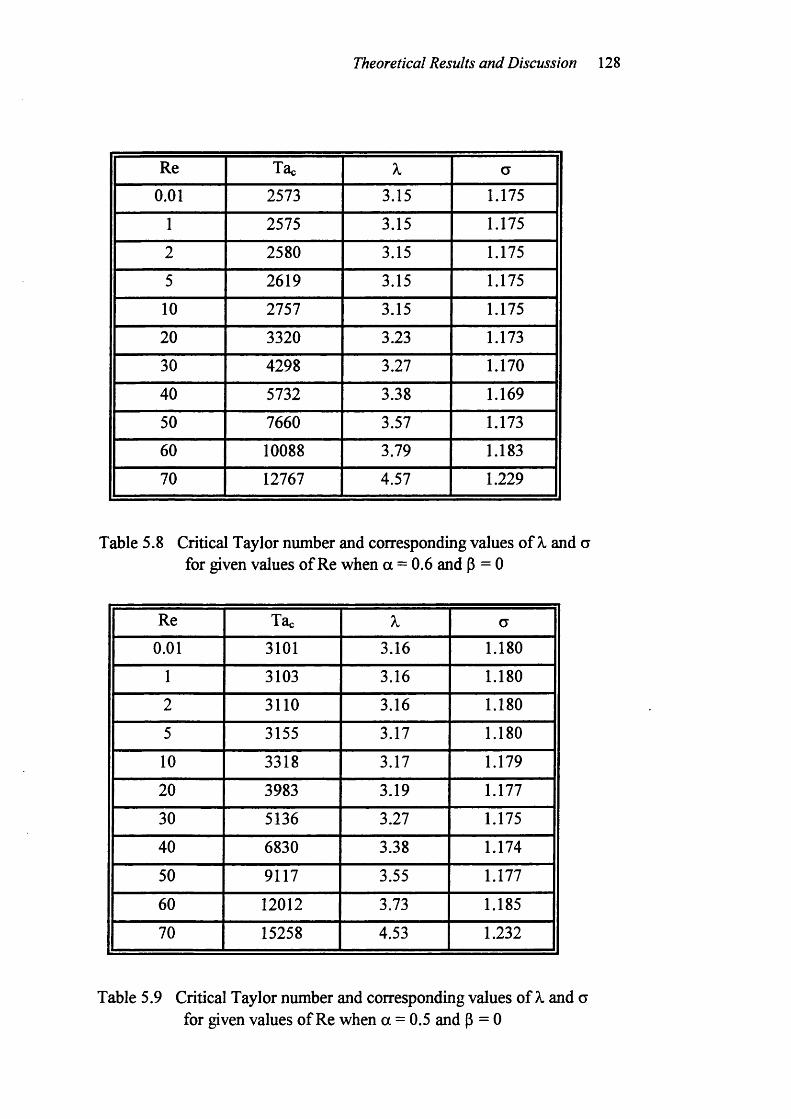
Theoretical Results and Discussion 128
Re Tac X a
0.01 2573 3.15 1.175
1 2575 3.15 1.175
2 2580 3.15 1.175
5 2619 3.15 1.175
10 2757 3.15 1.175
20 3320 3.23 1.173
30 4298 3.27 1.170
40 5732 3.38 1.169
50 7660 3.57 1.173
60 10088 3.79 1.183
70 12767 4.57 1.229
Table 5.8 Critical Taylor number and corresponding values of X and a for given values of Re when a = 0.6 and p = 0
Re Tac % a0.01 3101 3.16 1.180
1 3103 3.16 1.180
2 3110 3.16 1.180
5 3155 3.17 1.180
10 3318 3.17 1.179
20 3983 3.19 1.177
30 5136 3.27 1.175
40 6830 3.38 1.174
50 9117 3.55 1.177
60 12012 3.73 1.185
70 15258 4.53 1.232
Table 5.9 Critical Taylor number and corresponding values of X and afor given values of Re when a = 0.5 and P = 0
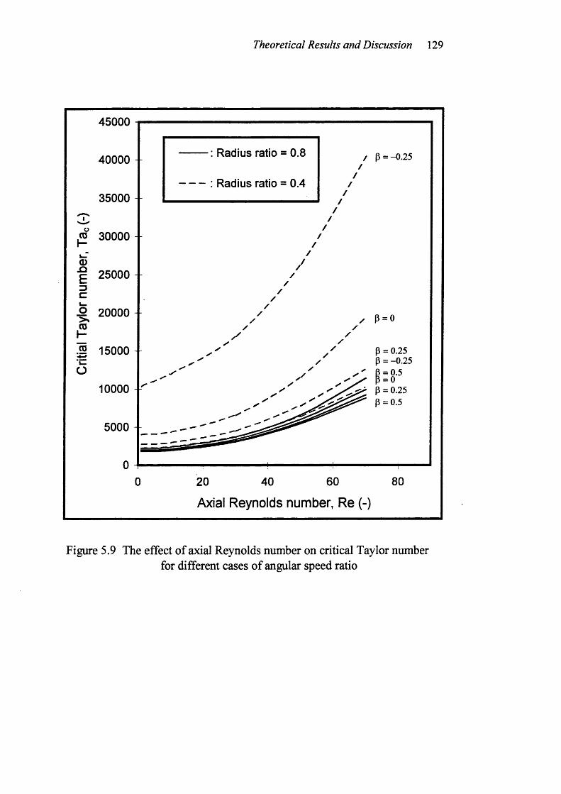
Theoretical Results and Discussion 129
45000
: Radius ratio = 0.8 P = -0.2540000 -
- ; Radius ratio = 0.435000
30000 -
25000 -
20000 - p = o
15000 - P = 0.25 P = -0.25 P = 0.5
P = 0.25 P = 0.5
10000
5000 -
20 40 60
Axial Reynolds number, Re (-)
Figure 5.9 The effect of axial Reynolds number on critical Taylor number for different cases of angular speed ratio
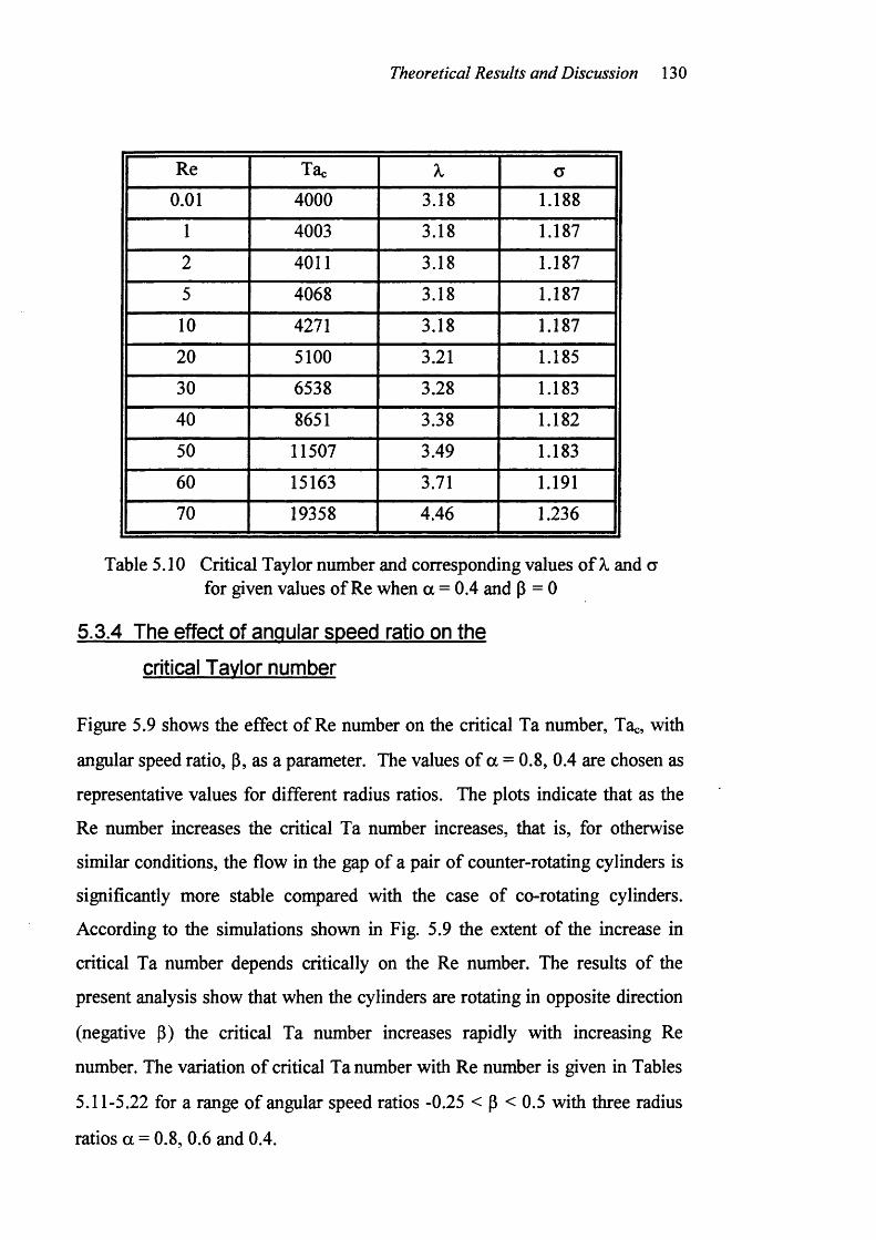
Theoretical Results and Discussion 130
Re Tac X a0.01 4000 3.18 1.188
1 4003 3.18 1.187
2 4011 3.18 1.187
5 4068 3.18 1.187
10 4271 3.18 1.187
20 5100 3.21 1.185
30 6538 3.28 1.183
40 8651 3.38 1.182
50 11507 3.49 1.183
60 15163 3.71 1.191
70 19358 4.46 1.236
Table 5.10 Critical Taylor number and corresponding values o f X and a for given values o f Re when a = 0.4 and p = 0
5.3.4 The effect of angular speed ratio on the
critical Tavlor number
Figure 5.9 shows the effect o f Re number on the critical Ta number, Ta«, with
angular speed ratio, p, as a parameter. The values of a = 0.8, 0.4 are chosen as
representative values for different radius ratios. The plots indicate that as the
Re number increases the critical Ta number increases, that is, for otherwise
similar conditions, the flow in the gap of a pair of counter-rotating cylinders is
significantly more stable compared with the case of co-rotating cylinders.
According to the simulations shown in Fig. 5.9 the extent of the increase in
critical Ta number depends critically on the Re number. The results of the
present analysis show that when the cylinders are rotating in opposite direction
(negative p) the critical Ta number increases rapidly with increasing Re
number. The variation o f critical Ta number with Re number is given in Tables
5.11-5.22 for a range of angular speed ratios -0.25 < p < 0.5 with three radius
ratios a = 0.8, 0.6 and 0.4.
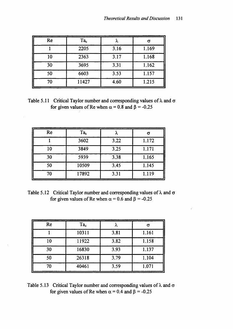
Theoretical Results and Discussion 131
Re Tac X a
1 2205 3.16 1.169
10 2363 3.17 1.168
30 3695 3.31 1.162
50 6603 3.53 1.157
70 11427 4.60 1.215
Table 5.11 Critical Taylor number and corresponding values o f X and a for given values of Re when a = 0.8 and P = -0.25
Re Tac X a1 3602 3.22 1.172
10 3849 3.25 1.171
30 5939 3.38 1.165
50 10509 3.45 1.145
70 17892 3.31 1.119
Table 5.12 Critical Taylor number and corresponding values o f X and a for given values of Re when a = 0.6 and p = -0.25
Re Tac X a
1 10311 3.81 1.161
10 11922 3.82 1.158
30 16830 3.93 1.137
50 26318 3.79 1.104
70 40461 3.59 1.071
Table 5.13 Critical Taylor number and corresponding values o f X and afor given values of Re when a = 0.4 and P = -0.25
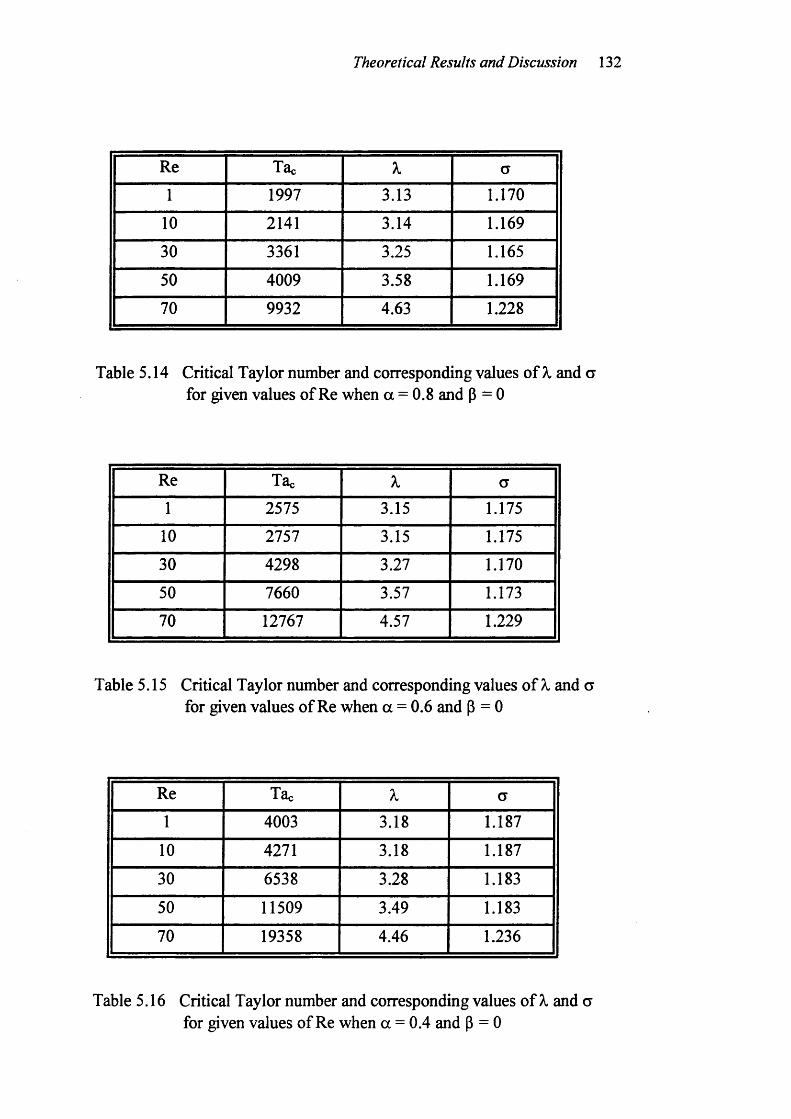
Theoretical Results and Discussion 132
Re Tac X a1 1997 3.13 1.170
10 2141 3.14 1.169
30 3361 3.25 1.165
50 4009 3.58 1.169
70 9932 4.63 1.228
Table 5.14 Critical Taylor number and corresponding values of X and a for given values o f Re when a = 0.8 and P = 0
Re Tac X a1 2575 3.15 1.175
10 2757 3.15 1.175
30 4298 3.27 1.170
50 7660 3.57 1.173
70 12767 4.57 1.229
T able 5.15 Critical T ay lor number and corresponding values o f X and a for given values o f Re when a = 0.6 and p = 0
Re Tac X a1 4003 3.18 1.187
10 4271 3.18 1.187
30 6538 3.28 1.183
50 11509 3.49 1.183
70 19358 4.46 1.236
Table 5.16 Critical Taylor number and corresponding values o f X and afor given values of Re when a = 0.4 and P = 0
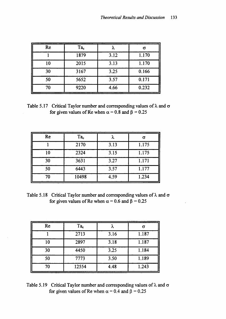
Theoretical Results and Discussion 133
Re Tac X a
1 1879 3.12 1.170
10 2015 3.13 1.170
30 3167 3.25 0.166
50 5652 3.57 0.171
70 9220 4.66 0.232
Table 5.17 Critical Taylor number and corresponding values o f X and a for given values o f Re when a = 0.8 and P = 0.25
Re Tac X a1 2170 3.13 1.175
10 2324 3.15 1.175
30 3631 3.27 1.171
50 6443 3.57 1.177
70 10498 4.59 1.234
Table 5.18 Critical Taylor number and corresponding values o f X and a for given values of Re when a = 0.6 and P = 0.25
Re Tac X a
1 2713 3.16 1.187
10 2897 3.18 1.187
30 4450 3.25 1.184
50 7773 3.50 1.189
70 12554 4.48 1.243
Table 5.19 Critical Taylor number and corresponding values o f X and afor given values of Re when a = 0.4 and P = 0.25
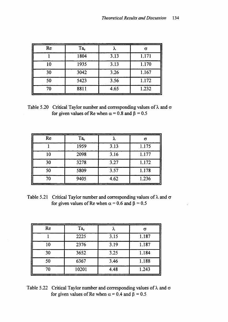
Theoretical Results and Discussion 134
Re Tac X a1 1804 3.13 1.171
10 1935 3.13 1.170
30 3042 3.26 1.167
50 5423 3.56 1.172
70 8811 4.65 1.232
Table 5.20 Critical Taylor number and corresponding values o f X and a for given values of Re when a = 0.8 and P = 0.5
Re Tac X CT
1 1959 3.13 1.175
10 2098 3.16 1.177
30 3278 3.27 1.172
50 5809 3.57 1.178
70 9405 4.62 1.236
Table 5.21 Critical Taylor number and corresponding values o f X and a for given values of Re when a = 0.6 and p = 0.5
Re Tac À a1 2225 3.15 1.187
10 2376 3.19 1.187
30 3652 3.25 1.184
50 6367 3.46 1.188
70 10201 4.48 1.243
Table 5.22 Critical Taylor number and corresponding values o f X and afor given values of Re when a = 0.4 and p = 0.5
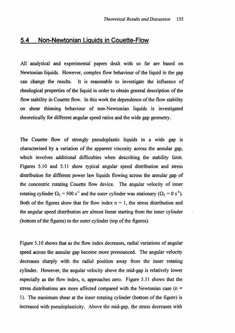
Theoretical Results and Discussion 135
5.4 Non-Newtonian Liquids in Couette-Flow
All analytical and experimental papers dealt with so far are based on
Newtonian liquids. However, complex flow behaviour o f the liquid in the gap
can change the results. It is reasonable to investigate the influence of
rheological properties o f the liquid in order to obtain general description o f the
flow stability in Couette flow. In this work the dependence of the flow stability
on shear thinning behaviour of non-Newtonian liquids is investigated
theoretically for different angular speed ratios and the wide gap geometry.
The Couette flow of strongly pseudoplastic liquids in a wide gap is
characterised by a variation o f the apparent viscosity across the annular gap,
which involves additional difficulties when describing the stability limit.
Figures 5.10 and 5.11 show typical angular speed distribution and stress
distribution for different power law liquids flowing across the annular gap of
the concentric rotating Couette flow device. The angular velocity o f inner
rotating cylinder Qi = 500 s" and the outer cylinder was stationary (O2 = 0 s' ).
Both of the figures show that for flow index n = 1, the stress distribution and
the angular speed distribution are almost linear starting fi*om the inner cylinder
(bottom of the figures) to the outer cylinder (top of the figures).
Figure 5.10 shows that as the flow index decreases, radial variations of angular
speed across the annular gap become more pronounced. The angular velocity
decreases sharply with the radial position away from the inner rotating
cylinder. However, the angular velocity above the mid-gap is relatively lower
especially as the flow index, n, approaches zero. Figure 5.11 shows that the
stress distributions are more affected compared with the Newtonian case (n =
1). The maximum shear at the inner rotating cylinder (bottom of the figure) is
increased with pseudoplasticity. Above the mid-gap, the stress decreases with
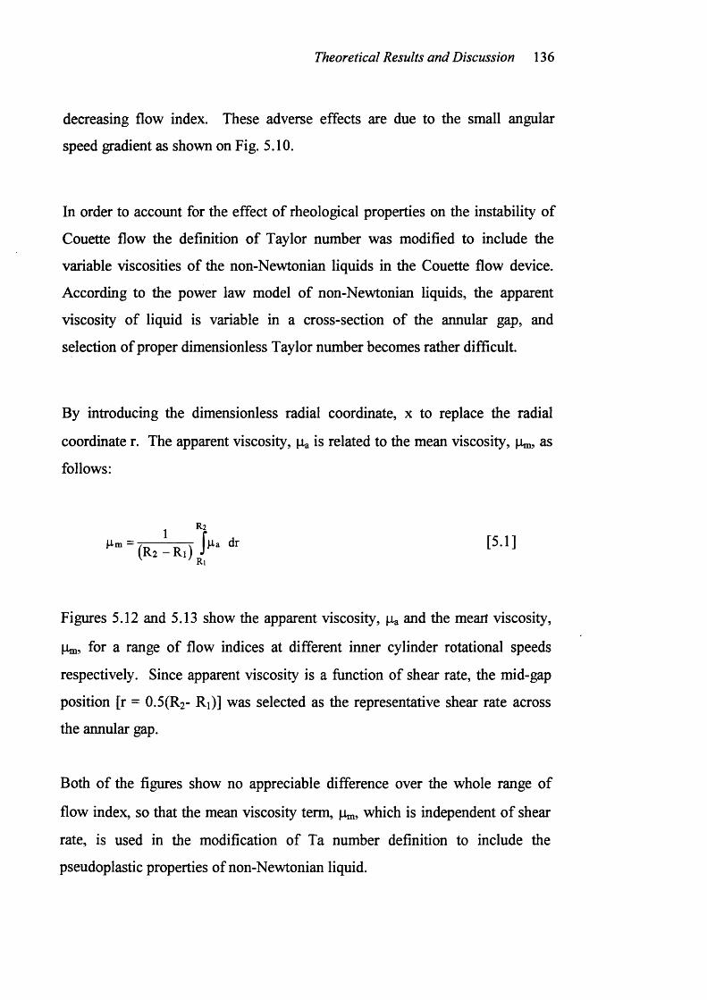
Theoretical Results and Discussion 13 6
decreasing flow index. These adverse effects are due to the small angular
speed gradient as shown on Fig. 5.10.
In order to account for the effect of rheological properties on the instability of
Couette flow the definition o f Taylor number was modified to include the
variable viscosities of the non-Newtonian liquids in the Couette flow device.
According to the power law model o f non-Newtonian liquids, the apparent
viscosity of liquid is variable in a cross-section of the annular gap, and
selection of proper dimensionless Taylor number becomes rather difficult.
By introducing the dimensionless radial coordinate, x to replace the radial
coordinate r. The apparent viscosity, Pa is related to the mean viscosity, as
follows:
1=
fJ g a dr [5.1]
(R 2-R i) r,
Figures 5.12 and 5.13 show the apparent viscosity, pa and the mean viscosity.
Pm, for a range of flow indices at different inner cylinder rotational speeds
respectively. Since apparent viscosity is a function of shear rate, the mid-gap
position [r = 0.5(R2- Ri)] was selected as the representative shear rate across
the annular gap.
Both of the figures show no appreciable difference over the whole range of
flow index, so that the mean viscosity term, pm, which is independent o f shear
rate, is used in the modification of Ta number definition to include the
pseudoplastic properties of non-Newtonian liquid.
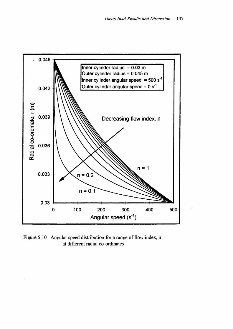
Theoretical Results and Discussion 13 7
(0c
I
0.045 1
0.042
© 0.039
g 0 036JD(00 1
0.033
0.03
Inner cylinder radius = 0.03 m Outer cylinder radius = 0.045 m Inner cylinder angular speed = 500 s" Outer cylinder angular speed = 0 s'^
Decreasing flow Index, n
100 200 300 400
Angular speed (s' )
n = 0.1
500
Figure 5.10 Angular speed distribution for a range of flow index, n at different radial co-ordinates
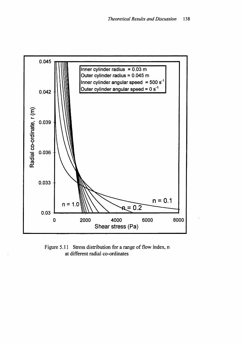
Theoretical Results and Discussion 13 8
0.045Inner cylinder radius = 0.03 m Outer cylinder radius = 0.045 m Inner cylinder angular speed = 500 s Outer cylinder angular speed = 0 s'^0.042
EL-
0.039(0c
0.033
= 0.20.03
800060000 2000 4000Shear stress (Pa)
Figure 5.11 Stress distribution for a range of flow index, n at different radial co-ordinates
Theoretical Results and Discussion 139
Inner cylinder radius = 0.03 m Outer cylinder radius = 0.045 m0.9
0.8
0.7
0.6 - -
0.5
0.4
0.2200 rpm
300 rpm500 rpm 900 rpm
0.2 0.4 0.6Flow Index, n (-)
0.8
Figure 5.12 Apparent viscosity for a range of flow index, n at different inner cylinder rotational speeds(Assume viscosity = IPa s“ when n = 1)
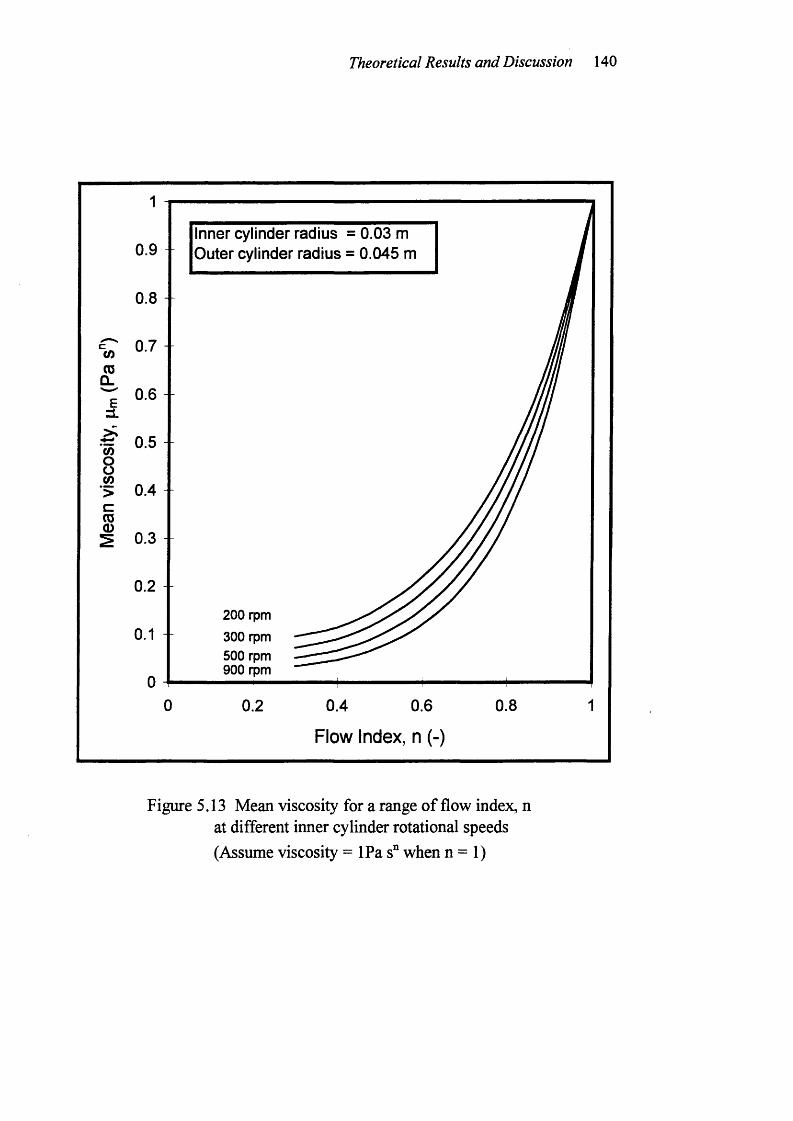
Theoretical Results and Discussion 140
Inner cylinder radius = 0.03 m Outer cylinder radius = 0.045 m0.9
0.8 -
0.7 -
0.6 ■ ■
0.5 -
0.4
0.3 -
0.2
200 rpm 300 rpm500 rpm 900 rpm
0.4 0.6
Flow Index, n (-)
0.80.2
Figure 5.13 Mean viscosity for a range of flow index, n at different inner cylinder rotational speeds(Assume viscosity = IPa s° when n = 1)
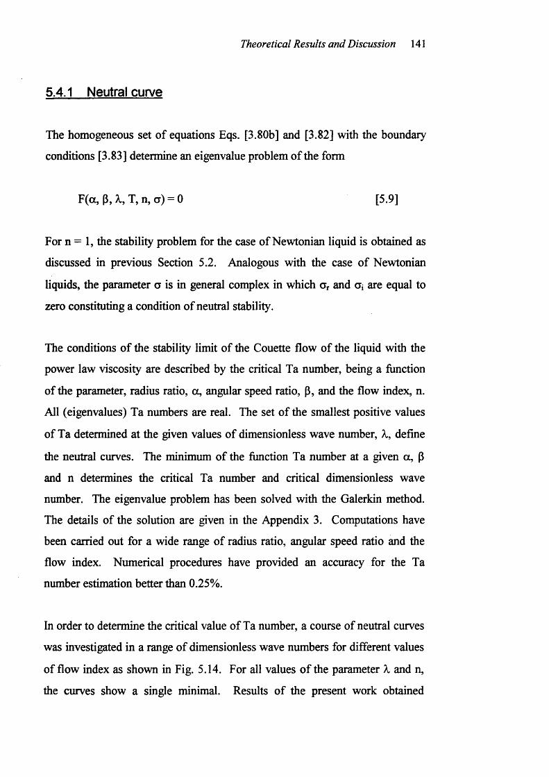
Theoretical Results and Discussion 141
5.4.1 Neutral curve
The homogeneous set o f equations Eqs. [3.80b] and [3.82] with the boundary
conditions [3.83] determine an eigenvalue problem of the form
F(a, p, T, n, a) = 0 [5.9]
For n = 1, the stability problem for the case of Newtonian liquid is obtained as
discussed in previous Section 5.2. Analogous with the case of Newtonian
liquids, the parameter a is in general complex in which Cr and ai are equal to
zero constituting a condition of neutral stability.
The conditions o f the stability limit of the Couette flow of the liquid with the
power law viscosity are described by the critical Ta number, being a function
of the parameter, radius ratio, a, angular speed ratio, P, and the flow index, n.
All (eigenvalues) Ta numbers are real. The set o f the smallest positive values
of Ta determined at the given values o f dimensionless wave number, A,, define
the neutral curves. The minimum of the function Ta number at a given a, p
and n determines the critical Ta number and critical dimensionless wave
number. The eigenvalue problem has been solved with the Galerkin method.
The details of the solution are given in the Appendix 3. Computations have
been carried out for a wide range of radius ratio, angular speed ratio and the
flow index. Numerical procedures have provided an accuracy for the Ta
number estimation better than 0.25%.
In order to determine the critical value of Ta number, a course of neutral curves
was investigated in a range of dimensionless wave numbers for different values
of flow index as shown in Fig. 5.14. For all values o f the parameter X and n,
the curves show a single minimal. Results o f the present work obtained
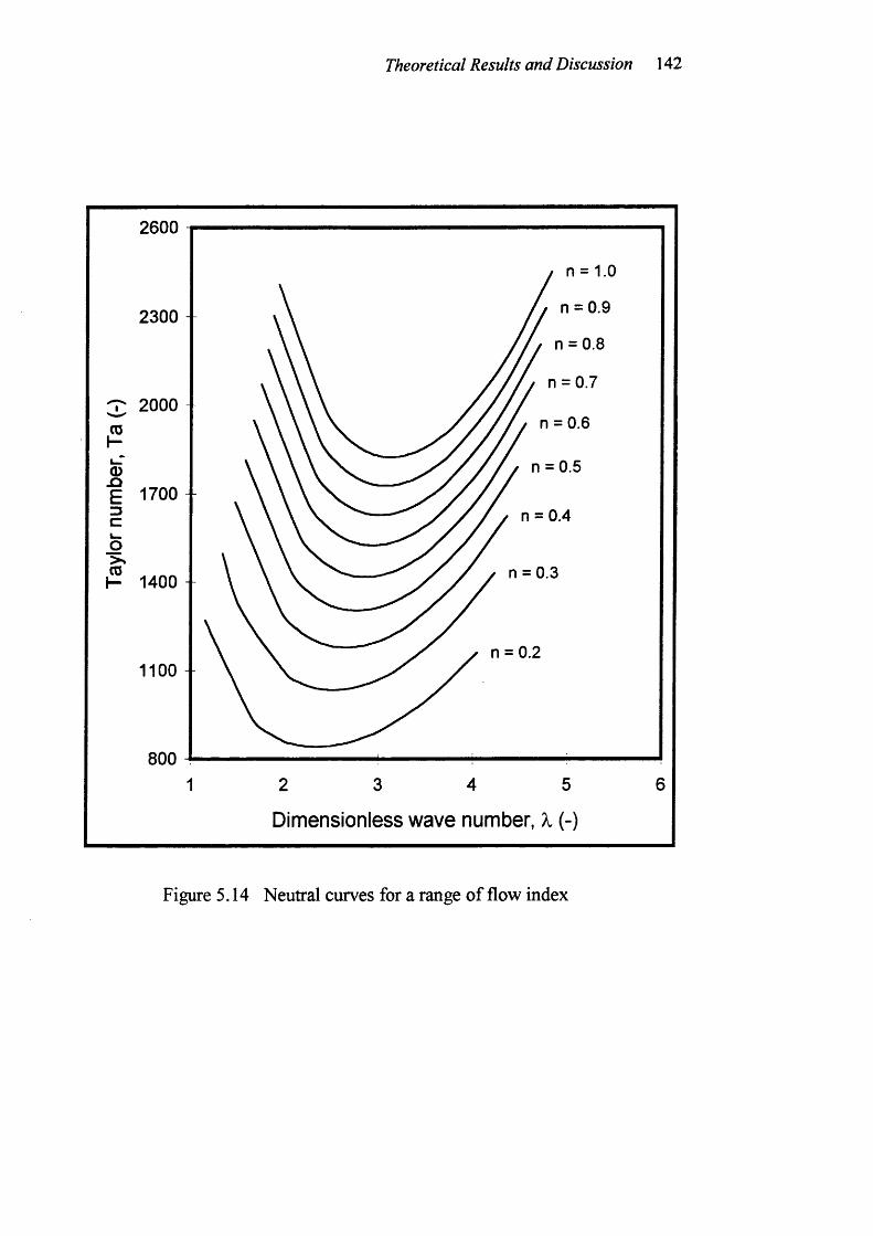
Theoretical Results and Discussion 142
2600 1
n = 0.92300 -n = 0.8
n = 0.72000
n = 0.6
n = 0.51700 -
n = 0.4
n = 0.31400 --
n = 0.21100
800 J
Dimensionless wave number, X (-)
Figure 5.14 Neutral curves for a range o f flow index
Theoretical Results and Discussion 143
6000 1n=1.0
n=0.9
5000 -n=0.8
n=0.74000 -
n=0.63000 - -
2000 - n=0.5
1000 - n=0.4
n=0,2 n=0.1n=0.3
Radius Ratio, a (-)
Figure 5.15 The effect o f the radius ratio on the critical Taylor number
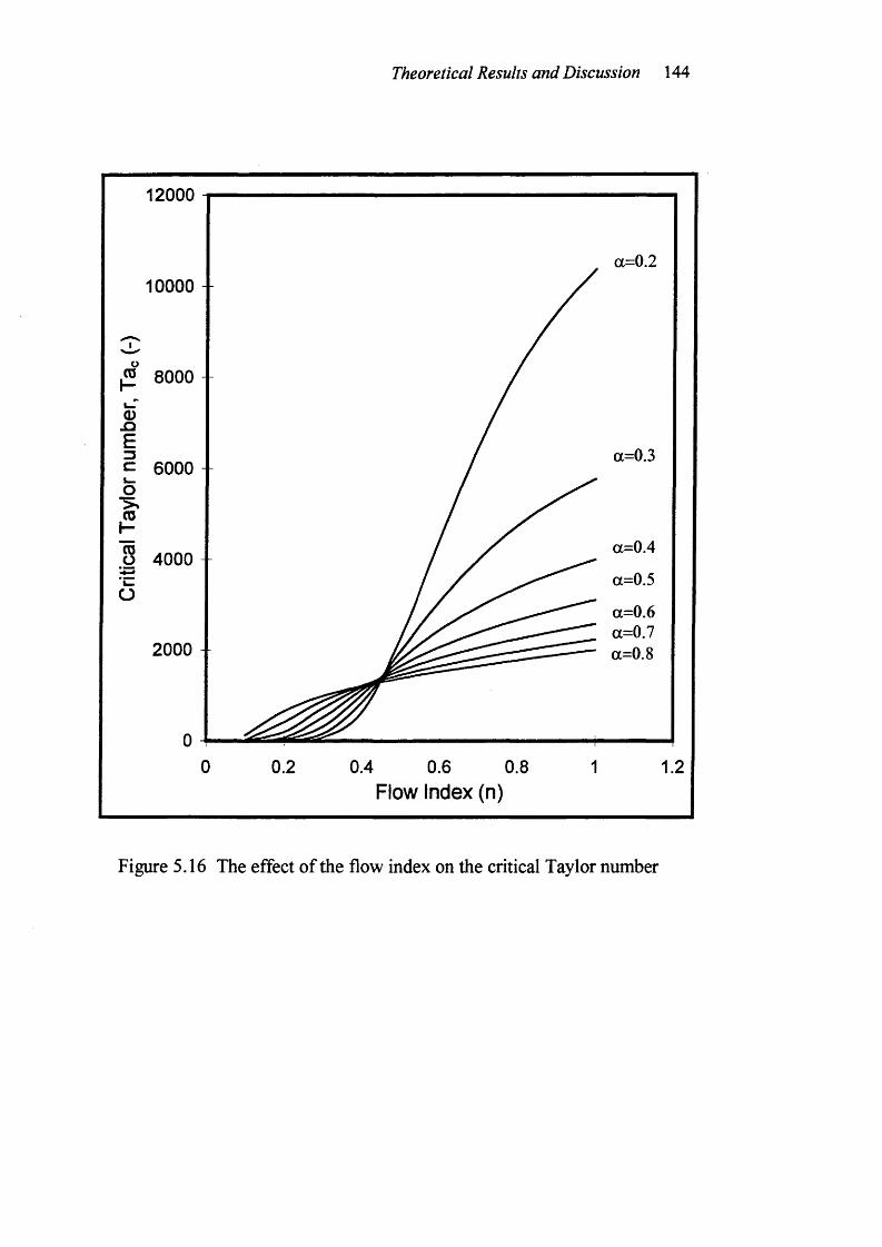
Theoretical Results and Discussion 144
12000
a=0.210000 -
8000 -
a=0.36000
>>
a=0.44000
a=0.6a=0.7a=0.82000 - -
0.2 0.4 0.6Flow Index (n)
0.8
Figure 5.16 The effect of the flow index on the critical Taylor number
Theoretical Results and Discussion 145
for n = 1 are in very good agreement with the earlier predictions (see Section
5.2). In the whole range o f flow index considered, the critical value of the Ta
number is an increasing function of n indicating that the shear thinning
properties o f the liquid generally has a destabilising influence on the flow.
5.4.2 The effect of radius ratio on the critical Tavlor number
Figure 5.15 shows the effect o f radius ratio, a, on the critical Ta number with
flow index, n, as a parameter at angular speed ratio, P = 0. The plot indicates
that the critical Ta number generally decreases as the flow index decreases over
the whole range o f radius ratio. Thus, for otherwise similar conditions, the
flow becomes less stable as shear thinning properties increase. According to
the simulations shown in Fig. 5.15 the extent o f the decreases in critical Ta
number also depends on the radius ratio.
Figure 5.16 is a cross plot o f the effect o f flow index on the critical Ta number
with radius ratio as a parameter. For flow index, n > 0.45 the critical Ta
number generally increases as the radius ratio decreases which is similar to the
case of Newtonian liquids as discussed in previous Section 5.2.3. However, for
n < 0.45, a different effect appears that is the critical Ta number increases as
the radius ratio increases. The variation of critical Ta number with flow index
is given in Tables 5.23-5.34 for a range of radius ratio 0.4 < a < 0.9 with a
range o f angular speed ratio together with dimensionless wave number. They
all show that the effect of rheology on the critical values is significant in all
cases and notably when n < 0.45. It should be noted that the predictions shown
in Fig. 5.16 are confirmed by the experimental RTD data obtained from the
coaxial cylinder apparatus as discussed later.
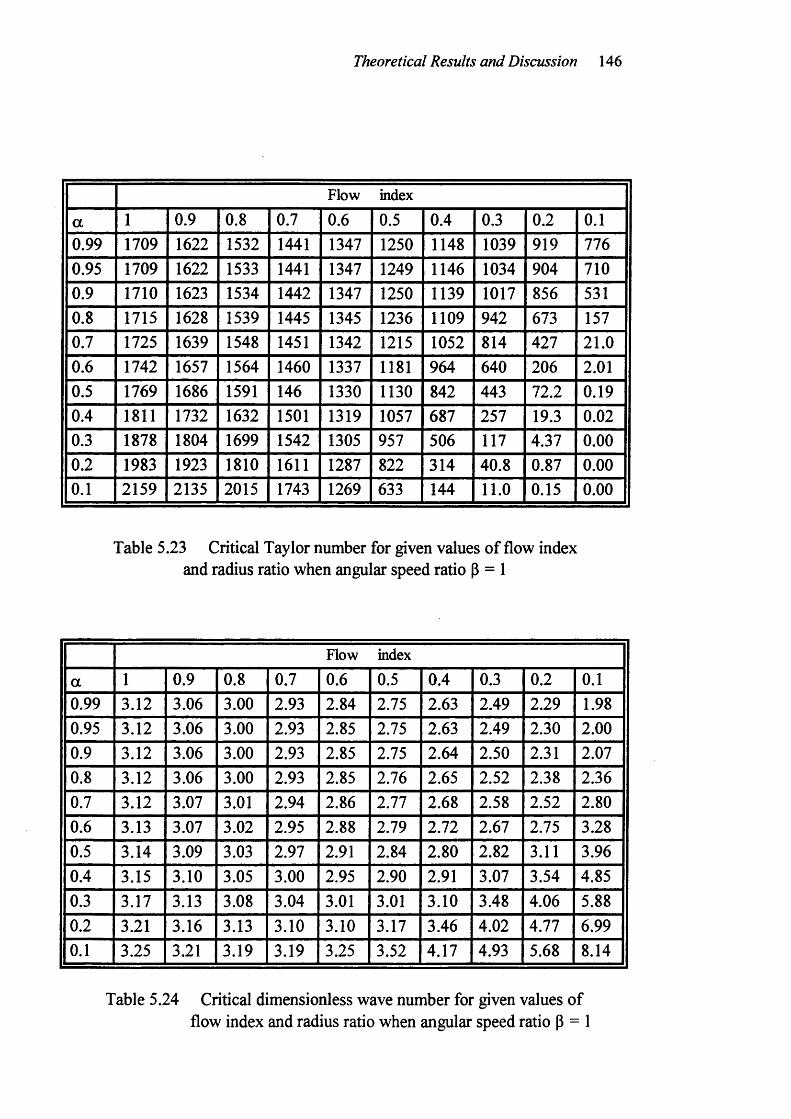
Theoretical Results and Discussion 146
Flow index
a 1 0.9 0.8 0.7 0.6 0.5 0.4 0.3 0.2 0.10.99 1709 1622 1532 1441 1347 1250 1148 1039 919 7760.95 1709 1622 1533 1441 1347 1249 1146 1034 904 7100.9 1710 1623 1534 1442 1347 1250 1139 1017 856 5310.8 1715 1628 1539 1445 1345 1236 1109 942 673 1570.7 1725 1639 1548 1451 1342 1215 1052 814 427 21.00.6 1742 1657 1564 1460 1337 1181 964 640 206 2.010.5 1769 1686 1591 146 1330 1130 842 443 72.2 0.190.4 1811 1732 1632 1501 1319 1057 687 257 19.3 0.020.3 1878 1804 1699 1542 1305 957 506 117 4.37 0.000.2 1983 1923 1810 1611 1287 822 314 40.8 0.87 0.000.1 2159 2135 2015 1743 1269 633 144 11.0 0.15 0.00
Table 5.23 Critical Taylor number for given values of flow index and radius ratio when angular speed ratio p = 1
Flow index
a 1 0.9 0.8 0.7 0.6 0.5 0.4 0.3 0.2 0.10.99 3.12 3.06 3.00 2.93 2.84 2.75 2.63 2.49 2.29 1.980.95 3.12 3.06 3.00 2.93 2.85 2.75 2.63 2.49 2.30 2.000.9 3.12 3.06 3.00 2.93 2.85 2.75 2.64 2.50 2.31 2.070.8 3.12 3.06 3.00 2.93 2.85 2.76 2.65 2.52 2.38 2.360.7 3.12 3.07 3.01 2.94 2.86 2.77 2.68 2.58 2.52 2.800.6 3.13 3.07 3.02 2.95 2.88 2.79 2.72 2.67 2.75 3.280.5 3.14 3.09 3.03 2.97 2.91 2.84 2.80 2.82 3.11 3.960.4 3.15 3.10 3.05 3.00 2.95 2.90 2.91 3.07 3.54 4.850.3 3.17 3.13 3.08 3.04 3.01 3.01 3.10 3.48 4.06 5.880.2 3.21 3.16 3.13 3.10 3.10 3.17 3.46 4.02 4.77 6.990.1 3.25 3.21 3.19 3.19 3.25 3.52 4.17 4.93 5.68 8.14
Table 5.24 Critical dimensionless wave number for given values offlow index and radius ratio when angular speed ratio P = 1
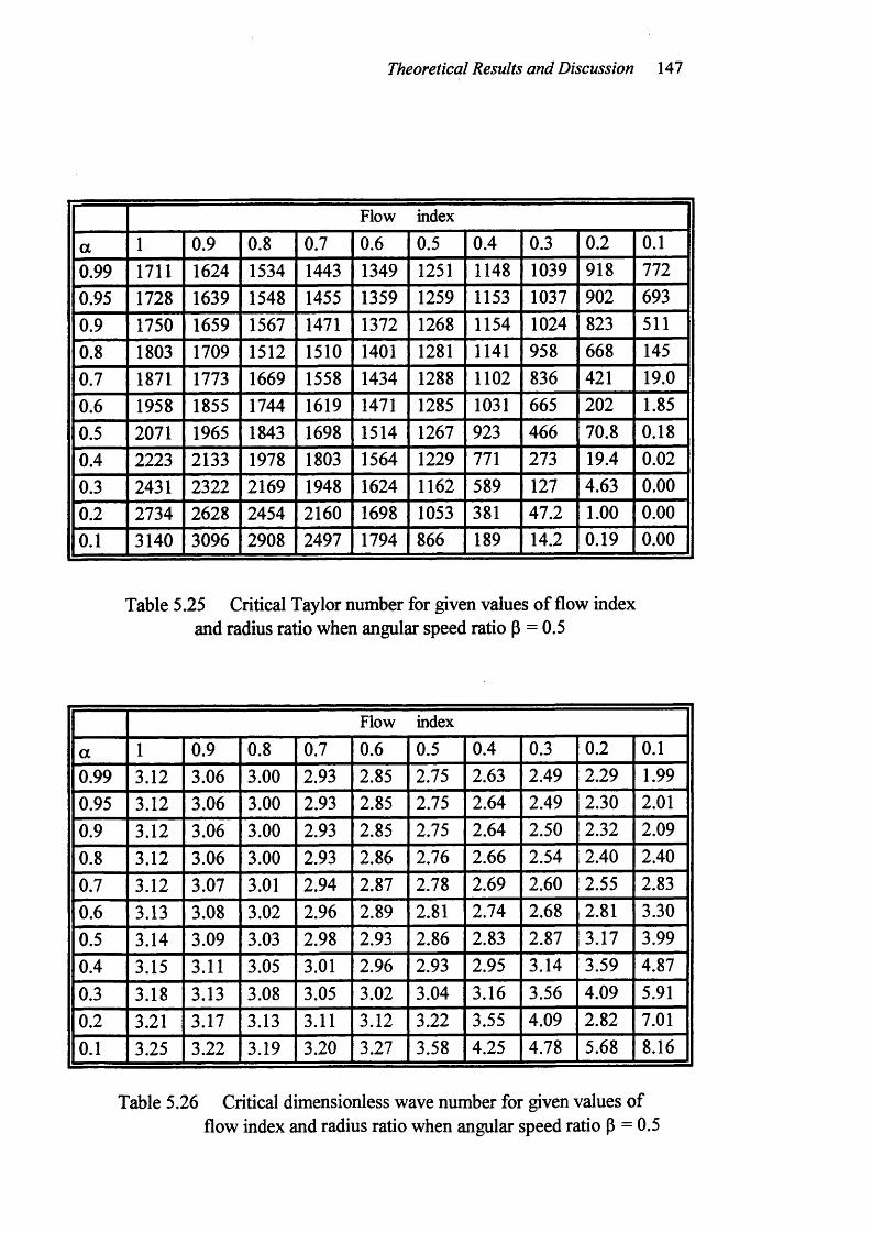
Theoretical Results and Discussion 147
Flow index
a 1 0.9 0.8 0.7 0.6 0.5 0.4 0.3 0.2 0.10.99 1711 1624 1534 1443 1349 1251 1148 1039 918 7720.95 1728 1639 1548 1455 1359 1259 1153 1037 902 6930.9 1750 1659 1567 1471 1372 1268 1154 1024 823 5110.8 1803 1709 1512 1510 1401 1281 1141 958 668 1450.7 1871 1773 1669 1558 1434 1288 1102 836 421 19.00.6 1958 1855 1744 1619 1471 1285 1031 665 202 1.850.5 2071 1965 1843 1698 1514 1267 923 466 70.8 0.180.4 2223 2133 1978 1803 1564 1229 771 273 19.4 0.020.3 2431 2322 2169 1948 1624 1162 589 127 4.63 0.000.2 2734 2628 2454 2160 1698 1053 381 47.2 1.00 0.000.1 3140 3096 2908 2497 1794 866 189 14.2 0.19 0.00
Table 5.25 Critical Taylor number for given values o f flow index and radius ratio when angular speed ratio p = 0.5
Flow index
a 1 0.9 0.8 0.7 0.6 0.5 0.4 0.3 0.2 0.10.99 3.12 3.06 3.00 2.93 2.85 2.75 2.63 2.49 2.29 1.990.95 3.12 3.06 3.00 2.93 2.85 2.75 2.64 2.49 2.30 2.010.9 3.12 3.06 3.00 2.93 2.85 2.75 2.64 2.50 2.32 2.090.8 3.12 3.06 3.00 2.93 2.86 2.76 2.66 2.54 2.40 2.400.7 3.12 3.07 3.01 2.94 2.87 2.78 2.69 2.60 2.55 2.830.6 3.13 3.08 3.02 2.96 2.89 2.81 2.74 2.68 2.81 3.300.5 3.14 3.09 3.03 2.98 2.93 2.86 2.83 2.87 3.17 3.990.4 3.15 3.11 3.05 3.01 2.96 2.93 2.95 3.14 3.59 4.870.3 3.18 3.13 3.08 3.05 3.02 3.04 3.16 3.56 4.09 5.910.2 3.21 3.17 3.13 3.11 3.12 3.22 3.55 4.09 2.82 7.010.1 3.25 3.22 3.19 3.20 3.27 3.58 4.25 4.78 5.68 8.16
Table 5.26 Critical dimensionless wave number for given values offlow index and radius ratio when angular speed ratio P = 0.5
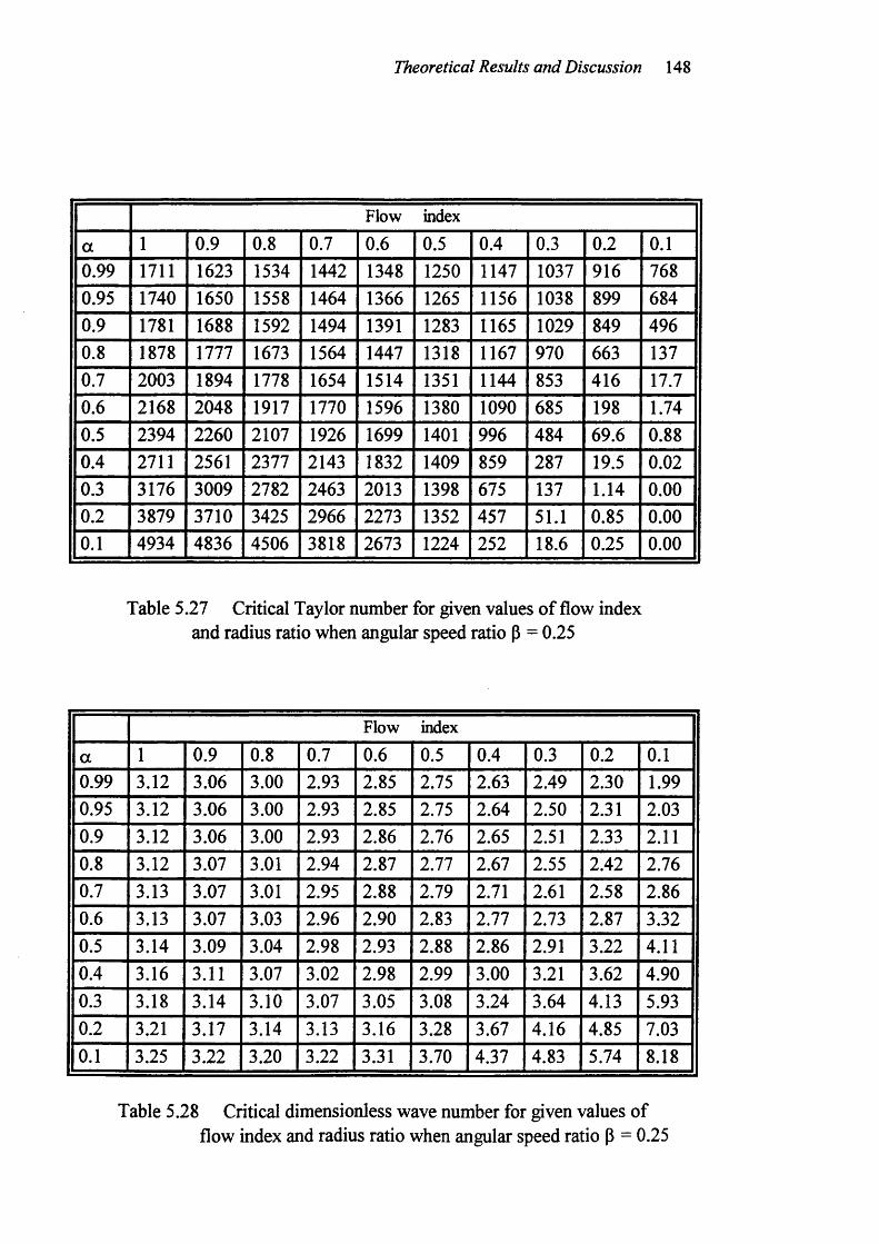
Theoretical Results and Discussion 148
Flow index
a 1 0.9 0.8 0.7 0.6 0.5 0.4 0.3 0.2 0.10.99 1711 1623 1534 1442 1348 1250 1147 1037 916 7680.95 1740 1650 1558 1464 1366 1265 1156 1038 899 6840.9 1781 1688 1592 1494 1391 1283 1165 1029 849 4960.8 1878 1777 1673 1564 1447 1318 1167 970 663 1370.7 2003 1894 1778 1654 1514 1351 1144 853 416 17.70.6 2168 2048 1917 1770 1596 1380 1090 685 198 1.740.5 2394 2260 2107 1926 1699 1401 996 484 69.6 0.880.4 2711 2561 2377 2143 1832 1409 859 287 19.5 0.020.3 3176 3009 2782 2463 2013 1398 675 137 1.14 0.000.2 3879 3710 3425 2966 2273 1352 457 51.1 0.85 0.000.1 4934 4836 4506 3818 2673 1224 252 18.6 0.25 0.00
Table 5.27 Critical Taylor number for given values of flow index and radius ratio when angular speed ratio P = 0.25
Flow index
a 1 0.9 0.8 0.7 0.6 0.5 0.4 0.3 0.2 0.10.99 3.12 3.06 3.00 2.93 2.85 2.75 2.63 2.49 2.30 1.990.95 3.12 3.06 3.00 2.93 2.85 2.75 2.64 2.50 2.31 2.030.9 3.12 3.06 3.00 2.93 2.86 2.76 2.65 2.51 2.33 2.110.8 3.12 3.07 3.01 2.94 2.87 2.77 2.67 2.55 2.42 2.760.7 3.13 3.07 3.01 2.95 2.88 2.79 2.71 2.61 2.58 2.860.6 3.13 3.07 3.03 2.96 2.90 2.83 2.77 2.73 2.87 3.320.5 3.14 3.09 3.04 2.98 2.93 2.88 2.86 2.91 3.22 4.110.4 3.16 3.11 3.07 3.02 2.98 2.99 3.00 3.21 3.62 4.900.3 3.18 3.14 3.10 3.07 3.05 3.08 3.24 3.64 4.13 5.930.2 3.21 3.17 3.14 3.13 3.16 3.28 3.67 4.16 4.85 7.030.1 3.25 3.22 3.20 3.22 3.31 3.70 4.37 4.83 5.74 8.18
Table 5.28 Critical dimensionless wave number for given values offlow index and radius ratio when angular speed ratio P = 0.25

Theoretical Results and Discussion 149
Flow index
a 1 0.9 0.8 0.7 0.6 0.5 0.4 0.3 0.2 0.10.99 1707 1620 1530 1439 1344 1246 1143 1033 941 7610.95 1756 1664 1571 1475 1375 1271 1160 1037 892 6660.9 1824 1727 1628 1525 1417 1303 1178 1033 841 4730.8 1995 1885 1767 1648 1518 1373 1203 985 653 1260.7 2231 2101 1963 1814 1647 1452 1209 878 4.8 16.00.6 2573 2414 2241 2047 1820 1544 1187 714 193 1.600.5 3101 2896 2664 2374 2066 1653 1126 512 67.8 0.170.4 4000 3713 3374 2960 2442 1790 1018 309 19.5 0.020.3 5778 5320 4747 4017 3091 1977 850 154 5.22 0.000.2 10375 9443 8189 6535 4477 2271 639 68.7 1.43 0.000.1 32549 29144 24042 17095 9114 2925 492 34.8 0.48 0.00
Table 5.29 Critical Taylor number for given values of flow index and radius ratio when angular speed ratio p = 0
Flow index
a 1 0.9 0.8 0.7 0.6 0.5 0.4 0.3 0.2 0.10.99 3.13 3.07 3.01 2.94 2.86 2.76 2.65 2.50 2.31 2.000.95 3.13 3.07 3.01 2.94 2.86 2.76 2.65 2.51 2.32 2.040.9 3.13 3.07 3.01 2.94 2.86 2.77 2.66 2.53 2.35 2.140.8 3.13 3.08 3.02 2.95 2.87 2.78 2.69 2.57 2.45 2.470.7 3.14 3.09 3.03 2.97 2.90 2.82 2.73 2.6 2.63 2.890.6 3.15 3.10 3.04 2.99 2.93 2.87 2.81 2.79 2.93 3.340.5 3.16 3.12 3.07 3.02 2.97 2.93 2.92 3.00 3.29 4.010.4 3.18 3.14 3.11 3.07 3.01 3.04 3.09 3.34 3.68 4.910.3 3.22 3.18 3.16 3.15 3.16 3.23 3.43 3.79 4.19 5.950.2 3.26 3.25 3.25 3.28 3.36 3.60 4.00 4.32 4.92 7.070.1 3.33 3.35 3.41 3.56 3.95 4.56 4.82 5.04 5.86 8.24
Table 5.30 Critical dimensionless wave number for given values offlow index and radius ratio when angular speed ratio P = 0
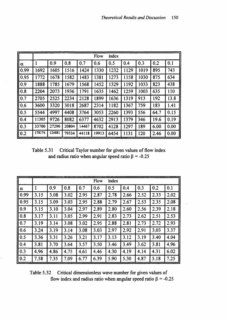
Theoretical Results and Discussion 150
Flow index
a 1 0.9 0.8 0.7 0.6 0.5 0.4 0.3 0.2 0.10.99 1692 1605 1516 1424 1330 1232 1129 1019 895 7430.95 1772 1678 1582 1483 1381 1273 1158 1030 875 6340.9 1888 1785 1679 1568 1452 1329 1192 1033 823 4380.8 2204 2073 1936 1791 1635 1462 1259 1003 635 1100.7 2705 2525 2234 2128 1899 1636 1319 913 192 13.80.6 3600 3320 3018 2687 2314 1182 1367 759 183 1.410.5 5544 4997 4408 3764 3053 2260 1393 556 64.7 0.150.4 11305 9726 8082 6377 4632 2913 1379 346 19.6 0.190.3 33700 27290 20804 14467 8702 4128 1297 189 6.00 0.000.2 178174 124881 79534 44118 19913 6454 1131 120 2.46 0.00
Table 5.31 Critical Taylor number for given values o f flow index and radius ratio when angular speed ratio P = -0.25
Flow index
a 1 0.9 0.8 0.7 0.6 0.5 0.4 0.3 0.2 0.10.99 3.15 3.08 3.02 2.95 2.87 2.78 2.66 2.52 2.33 2.020.95 3.15 3.09 3.03 2.95 2.88 2.79 2.67 2.53 2.35 2.080.9 3.15 3.10 3.04 2.97 2.89 2.80 2.60 2.56 2.39 2.180.8 3.17 3.11 3.05 2.99 2.91 2.83 2.73 2.62 2.51 2.530.7 3.19 3.14 3.08 3.02 2.95 2.88 2.81 2.73 2.72 2.930.6 3.24 3.19 3.14 3.08 3.03 2.97 2.92 2.91 3.03 3.370.5 3.36 3.31 3.26 3.21 3.17 3.13 3.12 3.19 3.40 4.040.4 3.81 3.70 3.64 3.57 3.50 3.46 3.49 3.62 3.81 4.960.3 4.96 4.86 4.75 4.61 4.46 4.30 4.19 4.14 4.31 6.020.2 7.58 7.35 7.09 6.77 6.39 5.90 5.30 4.87 5.18 7.25
Table 5.32 Critical dimensionless wave number for given values offlow index and radius ratio when angular speed ratio p = -0.25
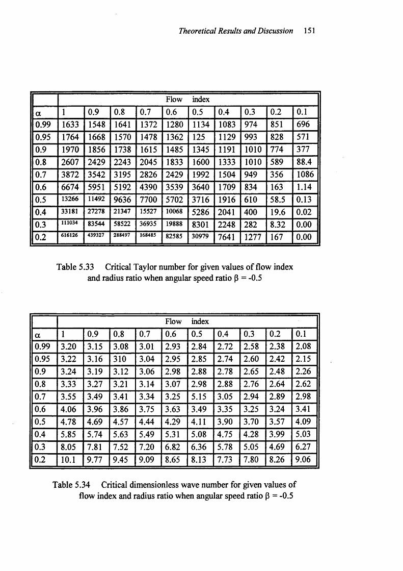
Theoretical Results and Discussion 151
Flow index
a 1 0.9 0.8 0.7 0.6 0.5 0.4 0.3 0.2 0.10.99 1633 1548 1641 1372 1280 1134 1083 974 851 6960.95 1764 1668 1570 1478 1362 125 1129 993 828 5710.9 1970 1856 1738 1615 1485 1345 1191 1010 774 3770.8 2607 2429 2243 2045 1833 1600 1333 1010 589 88.40.7 3872 3542 3195 2826 2429 1992 1504 949 356 10860.6 6674 5951 5192 4390 3539 3640 1709 834 163 1.140.5 13266 11492 9636 7700 5702 3716 1916 610 58.5 0.130.4 33181 27278 21347 15527 10068 5286 2041 400 19.6 0.020.3 111034 83544 58522 36935 19888 8301 2248 282 8.32 0.000.2 616126 439327 288497 168485 82585 30979 7641 1277 167 0.00
Table 5.33 Critical Taylor number for given values o f flow index and radius ratio when angular speed ratio p = -0.5
Flow index
a 1 0.9 0.8 0.7 0.6 0.5 0.4 0.3 0.2 0.10.99 3.20 3.15 3.08 3.01 2.93 2.84 2.72 2.58 2.38 2.080.95 3.22 3.16 310 3.04 2.95 2.85 2.74 2.60 2.42 2.150.9 3.24 3.19 3.12 3.06 2.98 2.88 2.78 2.65 2.48 2.260.8 3.33 3.27 3.21 3.14 3.07 2.98 2.88 2.76 2.64 2.620.7 3.55 3.49 3.41 3.34 3.25 5.15 3.05 2.94 2.89 2.980.6 4.06 3.96 3.86 3.75 3.63 3.49 3.35 3.25 3.24 3.410.5 4.78 4.69 4.57 4.44 4.29 4.11 3.90 3.70 3.57 4.090.4 5.85 5.74 5.63 5.49 5.31 5.08 4.75 4.28 3.99 5.030.3 8.05 7.81 7.52 7.20 6.82 6.36 5.78 5.05 4.69 6.270.2 10.1 9.77 9.45 9.09 8.65 8.13 7.73 7.80 8.26 9.06
Table 5.34 Critical dimensionless wave number for given values offlow index and radius ratio when angular speed ratio p = -0.5
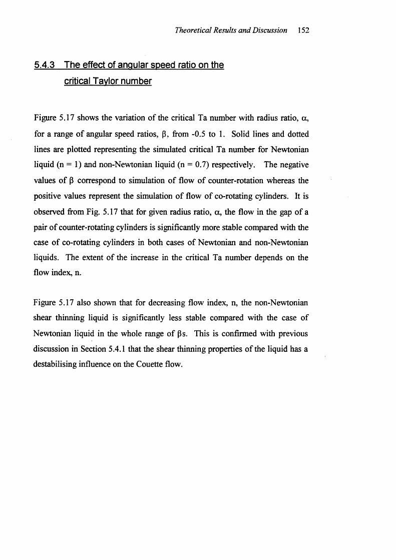
Theoretical Results and Discussion 152
5.4.3 The effect of angular speed ratio on the
critical Tavlor number
Figure 5.17 shows the variation of the critical Ta number with radius ratio, a,
for a range o f angular speed ratios, P, from -0.5 to 1. Solid lines and dotted
lines are plotted representing the simulated critical Ta number for Newtonian
liquid (n = 1) and non-Newtonian liquid (n = 0.7) respectively. The negative
values o f p correspond to simulation of flow o f counter-rotation whereas the
positive values represent the simulation of flow of co-rotating cylinders. It is
observed from Fig. 5.17 that for given radius ratio, a, the flow in the gap of a
pair o f counter-rotating cylinders is significantly more stable compared with the
case of co-rotating cylinders in both cases of Newtonian and non-Newtonian
liquids. The extent o f the increase in the critical Ta number depends on the
flow index, n.
Figure 5.17 also shown that for decreasing flow index, n, the non-Newtonian
shear thinning liquid is significantly less stable compared with the case of
Newtonian liquid in the whole range of ps. This is confirmed with previous
discussion in Section 5.4.1 that the shear thinning properties o f the liquid has a
destabilising influence on the Couette flow.
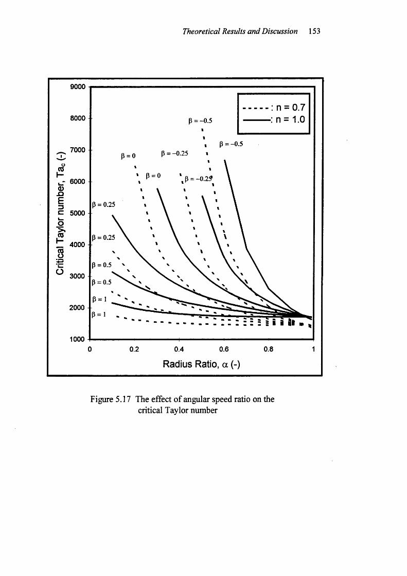
Theoretical Results and Discussion 153
9000
: n = 0.78000
P = -0.57000 P=-0.25p = o
p = o6000
P = 0.25C 5000
>»P = 0.25
L. 4000
P = 0.5
3000 -P = 0.5
2000
1000 J0.6 0.80.2 0.4
Radius Ratio, a (-)
Figure 5.17 The effect o f angular speed ratio on the critical Taylor number
Experimental Results and Discussion 154
CHAPTER SIX
EXPERIMENTAL RESULTS AND DISCUSSION
6.1 Introduction
In this section, experimental data are presented to assess the applicability o f the
axial dispersion model to the RTD of the different liquids in a Couette flow
device. The experiments show that the rheological effects could be significant,
and that this effect was not solely due to the fact the absolute value of the
apparent viscosity changes across the annular gap but also due to variation in
the power-law index. The experimental critical Taylor numbers are discussed
for a Newtonian liquid and the two non-Newtonian power-law liquids. Finally,
the experimental results will compared with the theoretical results presented in
Chapter 5.
6.2 Residence Time Distribution
6.2.1 Reproducibility
In the tracer stimulus-response experiments, there were several potential
sources o f error which could affect the RTD. Among these were the liquid feed
system, the tracer injection technique, the sampling frequency and period, and
slight fluctuations in the ambient temperature. It was not possible to estimate
the errors due to each individual source due to their mutual dependence.
Figure 6.1 and 6.2 show the Ce-curves for some of replicate experiments for
Newtonian and non-Newtonian liquids respectively. The reproducibility is
considered good. This suggested that the RTD and its parameters provided a
reliable tool for the analysis and interpretation of liquid transport in the Couette
flow devices. In the present study, each experiment was performed twice and
the values used were the mean.
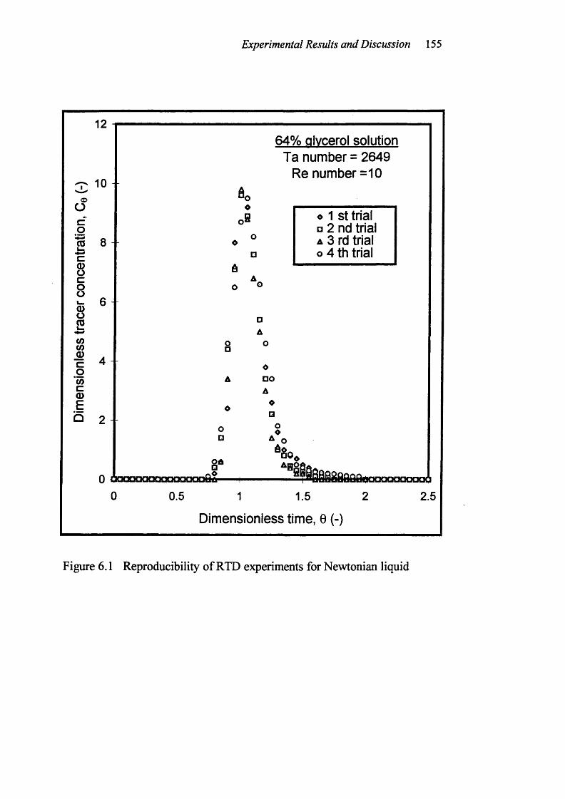
Experimental Results and Discussion 155
12 1
^ 10
oco% 8c8i e8COCOI 4gCOc(DEb 9
64% glycerol solution Ta number = 2649
Re number =10
ÔOo8 o 1 St trial
a 2nd trial* ° A 3 rd trial
□ o 4 th trial
o□oA
A□
0 O C X X X X X X X X X X X X X 3 9 a
0 0.5
06□O„ ^^i66fi88fiQ6»nnoaooaaa
1.5 2 2.5
Dimensionless time, 0 (-)
Figure 6.1 Reproducibility of RTD experiments for Newtonian liquid
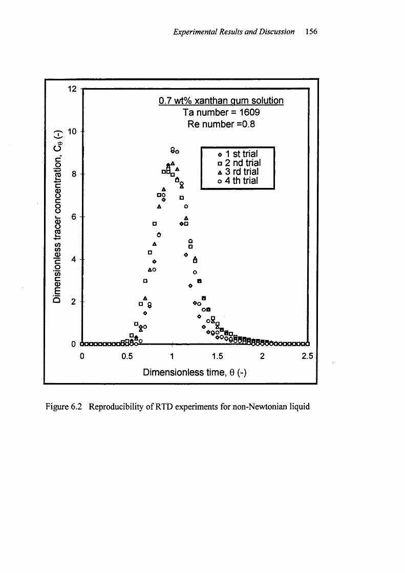
Experimental Results and Discussion 156
8CO
12 1
10<x>
Oco2 8 c8c
6 -
c 4g(/)cQ)Eb 2
0.7 wt% xanthan gum solution Ta number = 1609
Re number =0.8
8oA
A□OoA
AAO
o 1 St trial a 2 n d trial A 3 rd trial o 4 th trial
A
□A
AO
A□ 8
A
âO
I►
A coa
\ \
0 oocmooooaBBÔoS.
0 0.5 1—2§BSBB88a06oooooooi
1.5 2 2.5
Dimensionless time, 0 (-)
Figure 6.2 Reproducibility of RTD experiments for non-Newtonian liquid
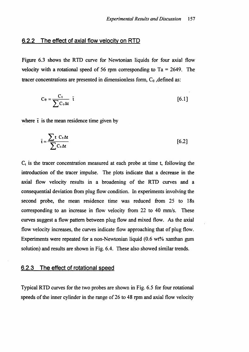
Experimental Results and Discussion 15 7
6.2.2 The effect of axial flow velocity on RTD
Figure 6.3 shows the RTD curve for Newtonian liquids for four axial flow
velocity with a rotational speed o f 56 rpm corresponding to Ta = 2649. The
tracer concentrations are presented in dimensionless form, Ce ,defined as:
t [6 .1 ]^C tA t
where t is the mean residence time given by
Ct is the tracer concentration measured at each probe at time t, following the
introduction of the tracer impulse. The plots indicate that a decrease in the
axial flow velocity results in a broadening o f the RTD curves and a
consequential deviation from plug flow condition. In experiments involving the
second probe, the mean residence time was reduced from 25 to 18s
corresponding to an increase in flow velocity from 22 to 40 mm/s. These
curves suggest a flow pattern between plug flow and mixed flow. As the axial
flow velocity increases, the curves indicate flow approaching that o f plug flow.
Experiments were repeated for a non-Newtonian liquid (0.6 wt% xanthan gum
solution) and results are shown in Fig. 6.4. These also showed similar trends.
6.2.3 The effect of rotational speed
Typical RTD curves for the two probes are shown in Fig. 6.5 for four rotational
speeds of the inner cylinder in the range of 26 to 48 rpm and axial flow velocity
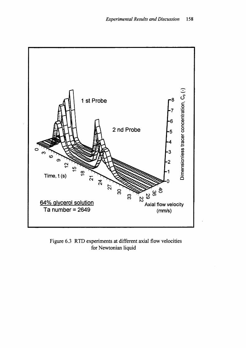
Experimental Results and Discussion 158
St Probe
nd Probe
oCO
O)CNI
L O
O O
Time, t (s)C N
C O o N) O) ro CD hOAxial flow velocity
oCO CO
CO64% glycerol solution
Ta number = 2649 (mm/s)
Figure 6.3 RTD experiments at different axial flow velocitiesfor Newtonian liquid
Experimental Results and Discussion 159
1 St Probe
2 nd Probe
Time, t (s) ^ csj
0.6 wt% xanthan gum solution Ta number = 1626
(DÜcg
Î888CD
0)
s.1COc0)E
Axial flow velocity (mm/s)
Figure 6.4 RTD experiments at different axial flow velocitiesfor non-Newtonian liquid (0.6 wt% xanthan gum solution)
Experimental Results and Discussion 160
o f 15 mm/s corresponding to an axial Reynolds number, Re = 10 and Taylor
numbers. Ta = 582, 958, 1429 and 1992 respectively. The theoretical critical
Taylor number, Ta for the present geometry (radius ratio = 0.67) was found to
be 2061 according to the eigenvalue of Eqs. [3.42a-b]. The figure shows that
the rotational speed critically affect the spread of the RTD. The Ce-curve for
rotational speed = 26 rpm in Fig. 6.5 shows the combined effect o f rotational-
axial flow on the RTD in the laminar flow regime. The other Ce-curve
corresponding to rotational speed = 48 rpm is very different. Narrowing of the
Ce-curve is observed due to the occurrence of Taylor vortex which provides
evidence o f flow change away fi*om well-mixed to plug flow.
Also shown in Fig. 6.6 for comparison are the Ce-curves obtained for the cases
o f four higher rotational speeds of the inner cylinder in the range of 50 to 112
rpm at the same axial flow velocity (Re number = 10) and Ta number (Ta =
2139, 3608, 5883 and 10712 respectively). The figure shows that the rotational
speed significantly affects the spread o f the RTD curve. Kataoka et al. (1981)
suggested that when Ta exceeded Ta , the plug flow condition could not be
maintained owing to the occurrence of longitudinal mixing over the vortices
boundary. It was attributable to the development the wavy Taylor-Couette
flow.
Similar experiments were carried out for a non-Newtonian liquid (0.6 wt%
xanthan gum solution) in Figs. 6.7 and 6.8. The plots show similar trends
observed for Newtonian fluids. The theoretical critical Ta number was found
to be 973 for a flow index n = 0.285. It is interesting to note that the mean
residence times are approximately the same for all rotational speeds examined.
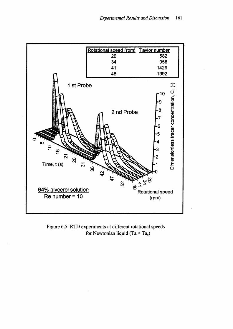
Experimental Results and Discussion 161
Rotational speed from) Tavlor number26 58234 95841 142948 1992
1 St Probe
Probe
Time, t (s)
W O)
Œ>Ücg
1888(DCOScgCO
5E
64% glycerol solution Re number = 10
Rotational speed (rpm)
Figure 6.5 RTD experiments at different rotational speedsfor Newtonian liquid (Ta < Ta )
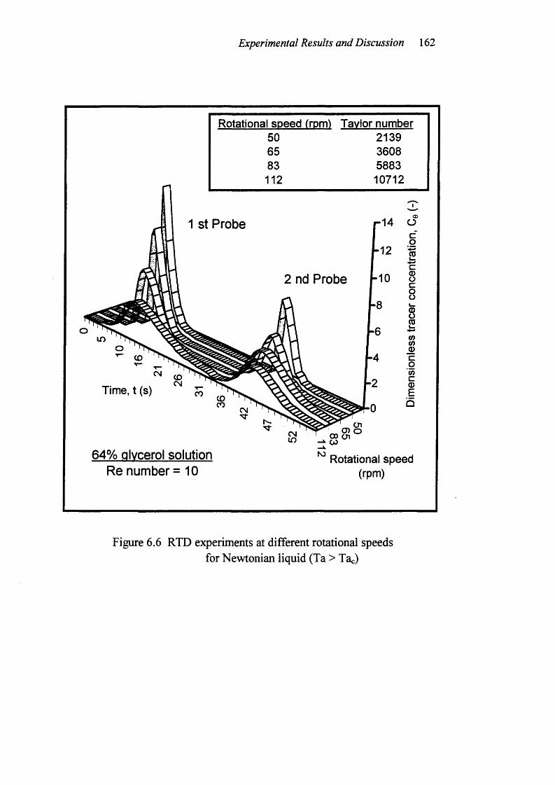
Experimental Results and Discussion 162
Rotational speed from) Tavlor number50 213965 360883 5883112 10712
1 St Probe
2 nd Probe
00 cn
Time, t (s)
Œ>0cq2
188CD
CO
si(OcCDE
64% Qlvcerol solution Re number = 10
Rotational speed (rpm)
Figure 6.6 RTD experiments at different rotational speedsfor Newtonian liquid (Ta > Ta )
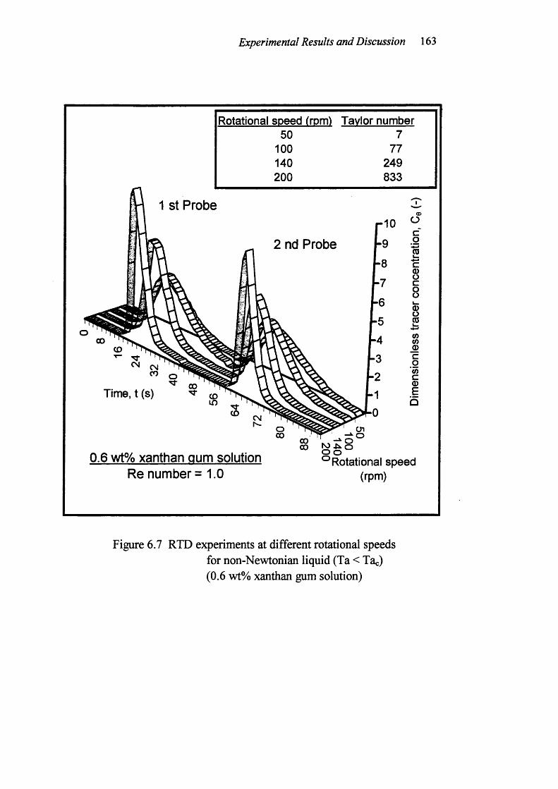
Experimental Results and Discussion 163
Rotational speed (rpm) Tavlor number
100140200
249833
St Probe
2 nd Probe
GO
CSJ CN ^
oOO
Time, t (s)
SCNt
§§8 g | 8
^Rotational speed (rpm)
0.6 wt% xanthan gum solution Re number = 1.0
Figure 6.7 RTD experiments at different rotational speedsfor non-Newtonian liquid (Ta < Tac)(0.6 wt% xanthan gum solution)
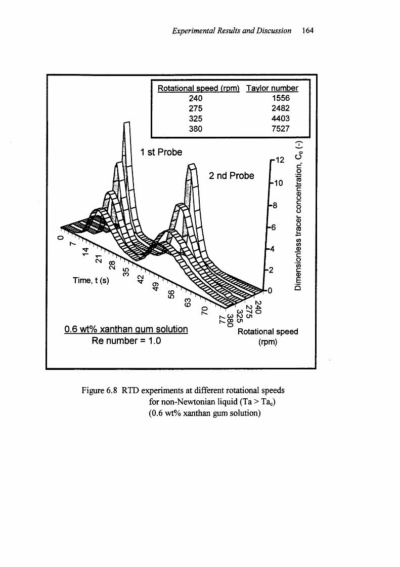
Experimental Results and Discussion 164
Rotational speed (rpm) 240 275 325 380
Tavlor number 1556 2482 4403 7527
1 S t Probe
2 nd Probe
tv. go cn
Time, t (s)
oco2c888(D0)CO0)coCOc0)E
0.6 wt% xanthan cum solution Re number = 1.0
Rotational speed (rpm)
Figure 6.8 RTD experiments at different rotational speedsfor non-Newtonian liquid (Ta > Tac)(0.6 wt% xanthan gum solution)
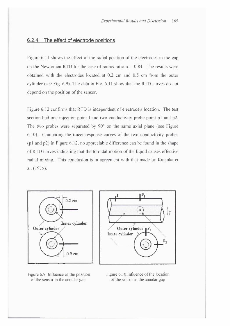
Experimental Results and Discussion 165
6.2.4 The effect of electrode positions
Figure 6.11 shows the effect of the radial position o f the electrodes in the gap
on the Newtonian RTD for the case of radius ratio a = 0.84. The results were
obtained with the electrodes located at 0.2 cm and 0.5 cm from the outer
cylinder (see Fig. 6.9). The data in Fig. 6.11 show that the RTD curves do not
depend on the position o f the sensor.
Figure 6.12 confirms that RTD is independent o f electrode's location. The test
section had one injection point I and two conductivity probe point pi and p2.
The two probes were separated by 90° on the same axial plane (see Figure
6.10). Comparing the tracer-response curves of the two conductivity probes
(pi and p2) in Figure 6.12, no appreciable difference can be found in the shape
of RTD curves indicating that the toroidal motion o f the liquid causes effective
radial mixing. This conclusion is in agreement with that made by Kataoka et
al. (1975).
0.2 cm
Inner cylinderOuter cylinder
0.5 cm
/ Outer cylinder i P Inner cylinder
Figure 6.9 Influence of the position of the sensor in the annular gap
Figure 6.10 Influence of the location of the sensor in the annular gap
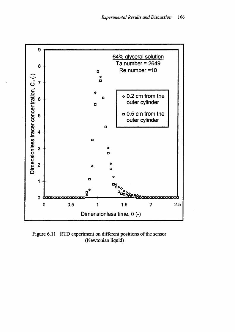
Experimental Results and Discussion 166
8
d 7Co 2 6
§I *m2 40)(/)•I 3o(O
b
64% qlvcerol solution Ta number = 2649
Re number =10«□
* 0.2 cm from the outer cylinder
□ 0.5 cm from the outer cylinder
□O0 qOOOOOCKKHDOOOOOO-0 0.5 1
I° P^^Sâ6ùooaoooaoocKH1.5 2.5
Dimensionless time, 0 (-)
Figure 6.11 RTD experiment on different positions of the sensor(Newtonian liquid)
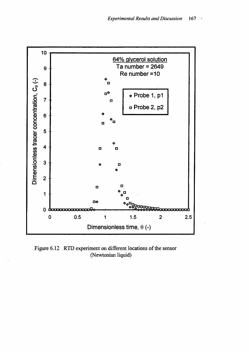
Experimental Results and Discussion 167
10
oÜC0
1c8C8I</)8coO)c0)Eb
9 +
8
7
6
5
4
3 +
2
1
64% Qlvcerol solution Ta number = 2649
Re number =10
o Probe 1, pi
□ Probe 2, p2
□
□o0 ooaDooooaaDaooa Oe j
0 0.5 1 1.5 2 2.5
Dimensionless time, 0 (-)
Figure 6.12 RTD experiment on different locations of the sensor(Newtonian liquid)
Experimental Results and Discussion 168
6.3 Axial Dispersion in Couette Flow
6.3.1 Axial dispersion model
An axial dispersion model is usually used to quantify the mixing performance
and the RTD curves of tracer material flowing through a Couette flow device.
The applicability of this model is based on several assumptions. The most
important o f these are:
1. Steady-state material flow conditions prevail and are not perturbed by the
introduction of the tracer stimulus.
2. Material holdup in the drum is independent o f axial position so that the
axial flow velocity o f the tracer is constant for fixed operating conditions.
3. Tracer concentration is uniform in each cross-section of the drum, i.e. it is
a function only of axial position and time.
4. The axial dispersion coefficient, which characterises axial transport of
tracer due to dispersive effect, is constant for fixed operating conditions.
The axial dispersion model for the tracer in its dimensionless form is
(Levenspiel, 1972)
aCe aCe 1 aXe r . -1
where 0, x. Ce correspond to dimensionless time, length, and tracer
concentration respectively. The dimensionless Peclet number is given by
P e ~ [6.4]
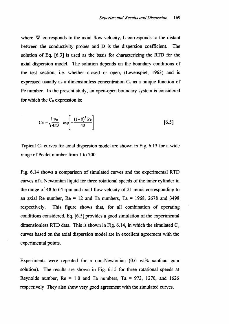
Experimental Results and Discussion 169
where W corresponds to the axial flow velocity, L corresponds to the distant
between the conductivity probes and D is the dispersion coefficient. The
solution o f Eq. [6.3] is used as the basis for characterizing the RTD for the
axial dispersion model. The solution depends on the boundary conditions of
the test section, i.e. whether closed or open, (Levenspiel, 1963) and is
expressed usually as a dimensionless concentration Ce as a unique function of
Pe number. In the present study, an open-open boundary system is considered
for which the Ce expression is:
(l-e)^Pe40
[6.5]
Typical Ce curves for axial dispersion model are shown in Fig. 6.13 for a wide
range o f Peclet number from 1 to 700.
Fig. 6.14 shows a comparison of simulated curves and the experimental RTD
curves o f a Newtonian liquid for three rotational speeds of the inner cylinder in
the range o f 48 to 64 rpm and axial flow velocity o f 21 mm/s corresponding to
an axial Re number. Re = 12 and Ta numbers. Ta = 1968, 2678 and 3498
respectively. This figure shows that, for all combination of operating
conditions considered, Eq. [6.5] provides a good simulation of the experimental
dimensionless RTD data. This is shown in Fig. 6.14, in which the simulated Ce
curves based on the axial dispersion model are in excellent agreement with the
experimental points.
Experiments were repeated for a non-Newtonian (0.6 wt% xanthan gum
solution). The results are shown in Fig. 6.15 for three rotational speeds at
Reynolds number. Re = 1.0 and Ta numbers. Ta = 973, 1270, and 1626
respectively They also show very good agreement with the simulated curves.
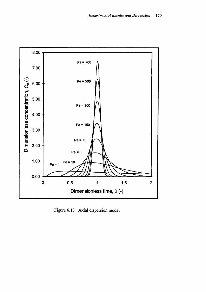
Experimental Results and Discussion 170
8.00 1
Pe = 700
7.00
Pe = 500CD 6.00 ■ ■
5.00 -Pe = 300
4.00 -
P e= 150c 3.00
Pe = 75E 2.00-
Pe = 30
1.00 Pe = 10Pe = 1
0.00 J0.5
Dimensionless time, 6 (-)
Figure 6.13 Axial dispersion model
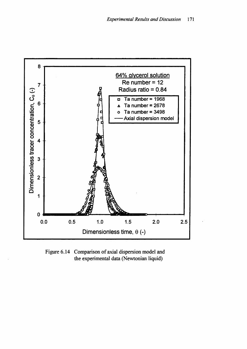
Experimental Results and Discussion 171
64% Qlvcerol solution Re number = 12
Radius ratio = 0.847
<D□ Ta number = 1968 A Ta number = 2678 o Ta number = 3498
Axial dispersion model
0.0 0.5 2.0 2.5
Dimensionless time, 0 (-)
Figure 6.14 Comparison of axial dispersion model andthe experimental data (Newtonian liquid)
Experimental Results and Discussion 172
0.6 wt% xanthan gum solution Re number = 1.0
Radius ratio = 0.84□ Ta number = 973 A Ta number = 1270 o Ta number = 1626 — Axial dispersion model
o
2.50.5
Dimensionless time, 0
Figure 6.15 Comparison of axial dispersion model andthe experimental data (non-Newtonian liquid)
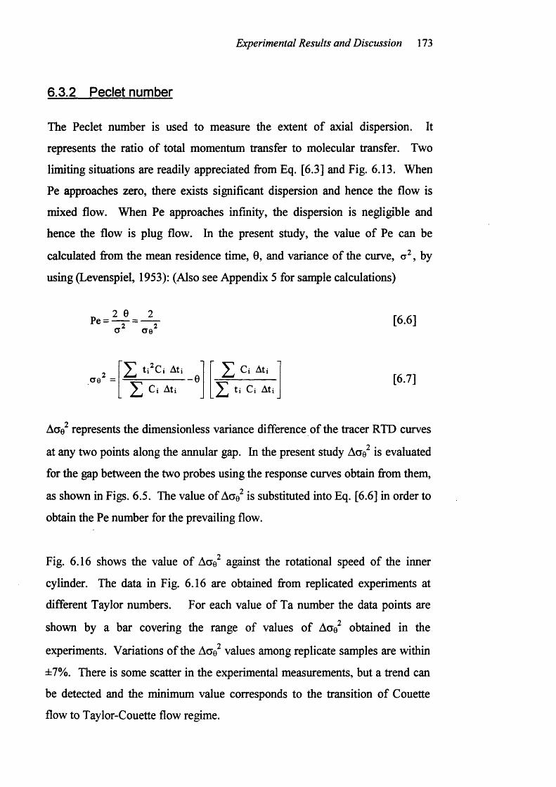
Experimental Results and Discussion 173
6.3.2 Peclet number
The Peclet number is used to measure the extent of axial dispersion. It
represents the ratio of total momentum transfer to molecular transfer. Two
limiting situations are readily appreciated from Eq. [6.3] and Fig. 6.13. When
Pe approaches zero, there exists significant dispersion and hence the flow is
mixed flow. When Pe approaches infinity, the dispersion is negligible and
hence the flow is plug flow. In the present study, the value of Pe can be
calculated from the mean residence time, 0, and variance of the curve, , by
using (Levenspiel, 1953): (Also see Appendix 5 for sample calculations)
y ti^Ci Ati ^ -0
^ Ci Ati
2 Ci Ati
y ti Ci Ati[6.7]
Aae represents the dimensionless variance difference of the tracer RTD curves
at any two points along the annular gap. In the present study Aae is evaluated
for the gap between the two probes using the response curves obtain from them,
as shown in Figs. 6.5. The value of Actg is substituted into Eq. [6.6] in order to
obtain the Pe number for the prevailing flow.
Fig. 6.16 shows the value of Aoe against the rotational speed of the inner
cylinder. The data in Fig. 6.16 are obtained from replicated experiments at
different Taylor numbers. For each value of Ta number the data points are
shown by a bar covering the range of values o f Aae obtained in the
experiments. Variations of the Aae values among replicate samples are within
±7%. There is some scatter in the experimental measurements, but a trend can
be detected and the minimum value corresponds to the transition of Couette
flow to Taylor-Couette flow regime.
Experimental Results and Discussion 174
I8§
0.018
0.016
0.014
0.012
0.01
0.008
8 c (U "C§CO
S 0.006c oCO
§ 0.004 E b
0.002 +
0 J20
64% Qvlcerol solution Radius ratio = 0.84
Re number = 12
30 40 50
Taylor number, Ta (-)
60 70
Figure 6.16 The effect of rotational speed of inner cylinder on dimensionless variance difference of the tracer RTD curve
Experimental Results and Discussion 175
The effect o f rotational speed on the Pe number for a Newtonian liquids (85%
glycerol solution), is shown in Fig. 6.17 for three axial flow rates expressed in
term of the axial Reynolds number. The plots in Fig. 6.17 show that as the
rotational speed o f the inner shaft increases, the Pe number increases fi’om an
initial value of about 100 to a maximum value of approximately 360 beyond
which any further increase in rotational speed causes a decrease in the Pe
number. The minimum and maximum values of the Pe number were found to
be functions o f the flow rate through the gap. In the present study the lowest
value of Pe was found to be about 80 corresponding to an axial flow velocity o f
26.4 mm/s (Re = 2) and the h ip est value o f Pe was 360 corresponding to an
axial flow velocity o f 39.6 mm/s (Re = 3) as shown in Fig. 6.17.
The variations in Pe number with increasing Ta number depicted in Fig. 6.17
suggests that significant deviation fi'om plug flow conditions can occur during
flow. Pudjiono e t a l (1992) and Pudjiono and Tavare (1993) in their recent
publications suggested that the maximum Pe number correspond to the critical
condition at which the Taylor vortices are fully developed.
Figures 6.17 to 6.30 show the results o f similar experiments carried out for
different geometrical and/or rheological parameters, summarized in Table 6.1.
They also show similar trends in data and confirm the results shown in Fig.
6.17.
Radius ratio, Newtonian liquids non-Newtonian liquids non-Newtonian liquidsR2/R] (Glycerol solution) (CMC solution) (Xanthan gum solution)0.84 Fig. 6.17 Fig. 6.23 Fig. 6.27
Fig. 6.18 Fig. 6.24 Fig. 6.28Fig. 6.19
0.67 Fig. 6.20 Fig. 6.25 Fig. 6.29Fig. 6.21 Fig. 6.26 Fig. 6.30Fig. 6.22
Table 6.1 Summary of the experimental Pe - Ta plots
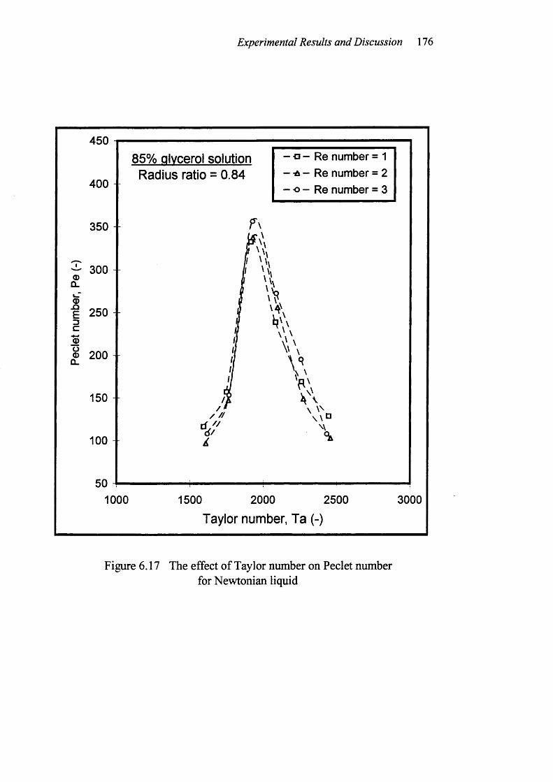
Experimental Results and Discussion 176
450 1- c - Re number = 1- -A - Re number = 2 - o - Re number = 3
85% glycerol solution Radius ratio = 0.84
400 -
350 -
300
250
200
150/ / /
d / /\ \ 0
100
50 -i— 1000 2000
Taylor number, Ta (-)2500 30001500
Figure 6.17 The effect of Taylor number on Peclet numberfor Newtonian liquid
Experimental Results and Discussion 177
500 1
450
400 -
X 350 +(D 0_fe 300
J DIc 250%Ü 0)0_ 200
150
100
50
64% glycerol solution Radius ratio = 0.84
- - Re number = 8 - Re number = 12
-■A - Re number = 18 - - 0 - Re number = 23- « - Re number = 27
f
1000 2000 3000 4000
Taylor number, Ta (-)
5000
Figure 6.18 The effect o f Taylor number on Peclet numberfor Newtonian liquid
Experimental Results and Discussion 178
550
500
450
400
S . 350
0)E 3003C
^ 250Ü<D
OL200
45% glycerol solution Radius ratio = 0.84
- -o - Re number = 35- -o - Re number = 50- -A - Re number = 58- -o - Re number = 62
V / V' \ \
/ / \
\ \\ \\ \\ \
I / / / \150- / / /
100 -
50
\ \\ \ \
\ \\ 4\ ^
\
\ \\
\
\ \\ \\ \
h o \\
5000 10000
Taylor number, Ta (-)15000
F igure 6.19 The effect of T ay lor number on Peclet numberfor Newtonian liquid
Experimental Results and Discussion 179
450
400 --
350 -
(D 300 Û.
L .3c%o 200 CL
150
100
50
85% glycerol solution Radius ratio = 0.67
- a - Re number = 1- -A - Re number = 2- o - Re number = 4
A
i//
/ / %
1000 2000 3000
Taylor number, Ta (-)4000
Figure 6.20 The effect of Taylor number on Peclet numberfor Newtonian liquid
Experimental Results and Discussion 180
350 1
E 200
64% glycerol solution Radius ratio = 0.67
- -a - Re number = 7Re number = 17
” -A - Re number = 22- o - Re number = 25- •* - Re number = 29
w ww ww \v\\ \ \.
M v .
"IK------O---- o
□
0 4000 8000 12000
Taylor number, Ta (-)
16000
Figure 6.21 The effect of Taylor number on Peclet numberfor Newtonian liquid
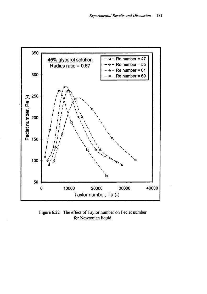
Experimental Results and Discussion 181
350
300 -
2500)CL
0)E 2003C0)8Û- 150
100
50
45% glycerol solution Radius ratio = 0.67
- d - Re number = 47Re number = 55
- -A “ Re number = 61 - o - Re number = 69
/
/P N // I / P/ / / /I I I /
/ ¥ /I I I I
6 / / /
I A VT/1 \\ f f V \ \
1111 \
\ \\ \
I
\ \\ \\ \\ \\ \ \
U VV
\
\
\\
\
10000 20000 30000Taylor number, Ta (-)
40000
Figure 6.22 The effect of Taylor number on Peclet numberfor Newtonian liquid
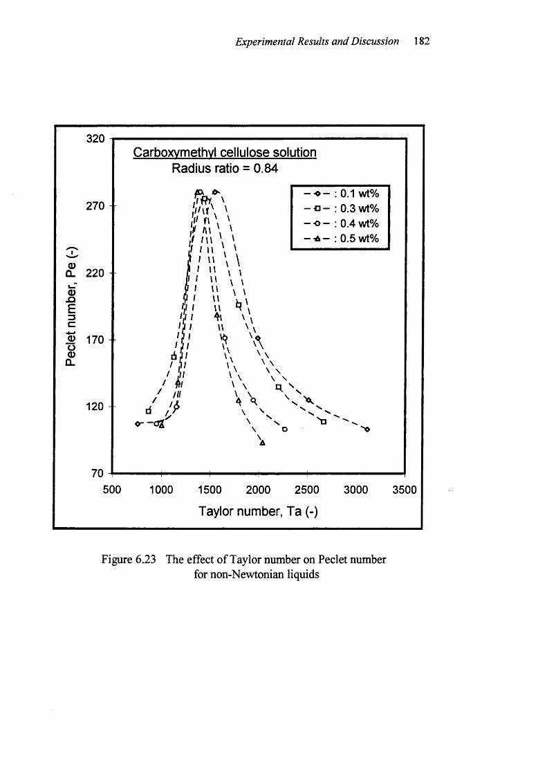
Experimental Results and Discussion 182
320
270 -
0)CL 220i_r0).aE3C
% 1708
CL
120
70
Carboxvmethvl cellulose solution Radius ratio = 0.84
fSX
h ''m \
— "O —— o —— o —— ^ —
0.1 wt% 0.3 wt% 0.4 wt% 0.5 wt%
500 1000 1500 2000 2500
Taylor number, Ta (-)
3000 3500
Figure 6.23 The effect of Taylor number on Peclet numberfor non-Newtonian liquids
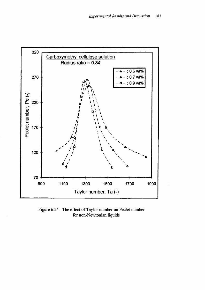
Experimental Results and Discussion 183
320
270
(DÛ. 220
5E3C
% 170 o(DQ_
120
Carboxvmethvl cellulose solution Radius ratio = 0.84
900
&•— -A — “ "O — — Cl —
0.6 wt% 0.7 wt% 0.9 wt%
11/I t//#I
/\//
il‘ " 'l i
/ /
\ \ \\ \ \\ \ \
\\ \ \\ \ \\ \ \
w \\ \ \
V\"\ \\ \
\b
1100 1300 1500 1700
Taylor number, Ta (-)
1900
Figure 6.24 The effect of Taylor number on Peclet numberfor non-Newtonian liquids
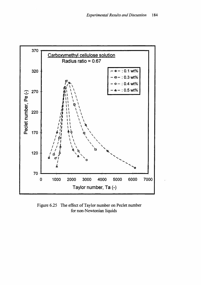
Experimental Results and Discussion 184
370
320 -
2700)Û.
<DE 220= 3C0)ÿO. 170
120 -
Carboxvmethvl cellulose solution Radius ratio = 0.67
r~ < — : 0.1 wt%
_ o — — " A —
0.3 wt% 0.4 wt% 0.5 wt%
1000 2000 3000 4000 5000 6000 7000
Taylor number, Ta (-)
Figure 6.25 The effect o f Taylor number on Peclet numberfor non-Newtonian liquids
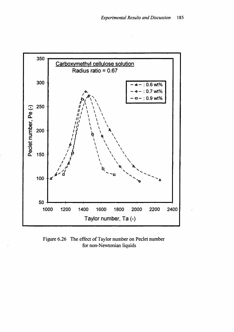
Experimental Results and Discussion 185
350
300
3 2500)Û.
E 2003C0)
0. 150
100
50
Carboxvmethvl cellulose solution Radius ratio = 0.67
0.6 wt% 0.7 wt% 0.9 wt%
i \ \ \\ \ \ \
?\\\\
\ \\ \\ \\ \\ \
\ \ \\ V.
1000 1200 1400 1600 1800 2000 2200 2400
Taylor number, Ta (-)
Figure 6.26 The effect of Taylor number on Peclet numberfor non-Newtonian liquids
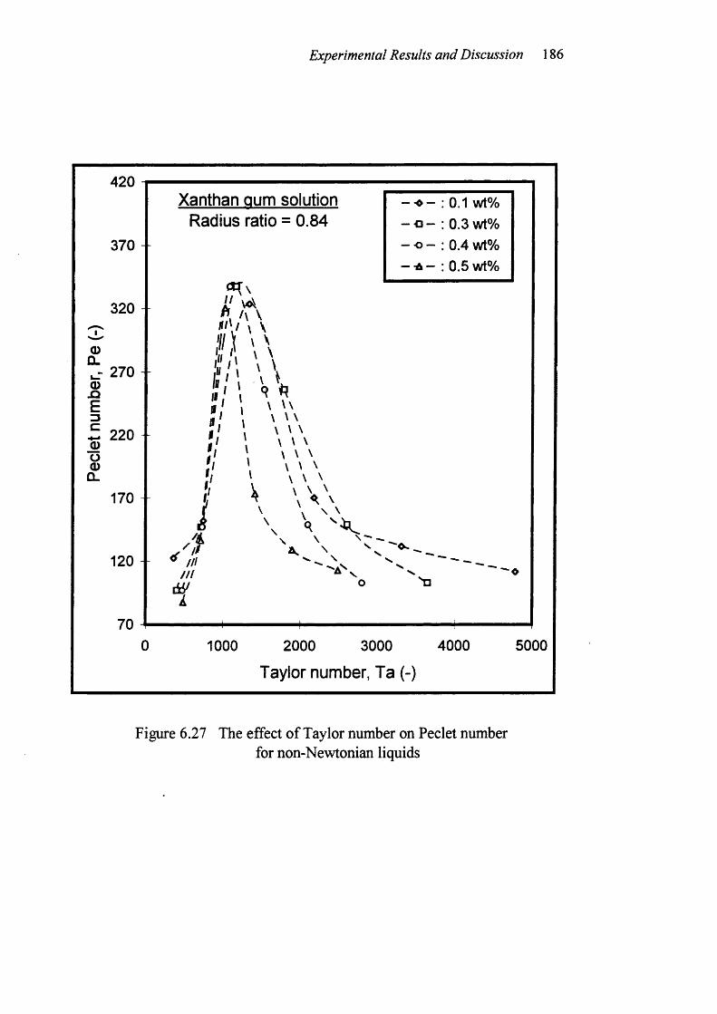
Experimental Results and Discussion 186
420
370 -
320
0)Q.
- 270Q)E3C%Ü0>Q_
220 -
170
120
70
Xanthan gum solution Radius ratio = 0.84
| / t \\ \II \\
9 'h\ w \ \ \\ \ \\ \ \\ \ \\ \ \\ \ \
if\
-o -o -
0.1 wt% 0.3 wt%
■” ■o — ; 0.4 wt% — -A — : 0.5 wt%
\ -\
/// ///
I '
\
1000 2000 3000 4000
Taylor number, Ta (-)
5000
Figure 6.27 The effect o f Taylor number on Peclet numberfor non-Newtonian liquids
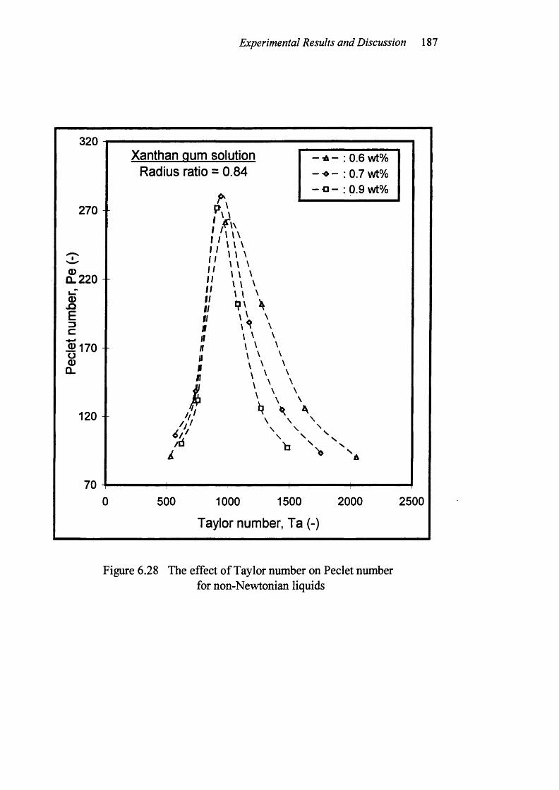
Experimental Results and Discussion 187
320
270
0)CL 220
iE3C
JW170ëCL
120
70
Xanthan gum solution Radius ratio = 0.84
k11I II I
I II II I
I II Itn
iIIfn
I
\ \ \\ \ \\ \ \\ \ \\ \ \
\\ \ \\ \ \ \ \ '
\ \
— -A — : 0.6 wt%— ! 0.7 wt%- a - : 0.9 wt%
k\ \ \
500 1000 1500 2000
Taylor number, Ta (-)
2500
Figure 6.28 The effect of Taylor number on Peclet numberfor non-Newtonian liquids
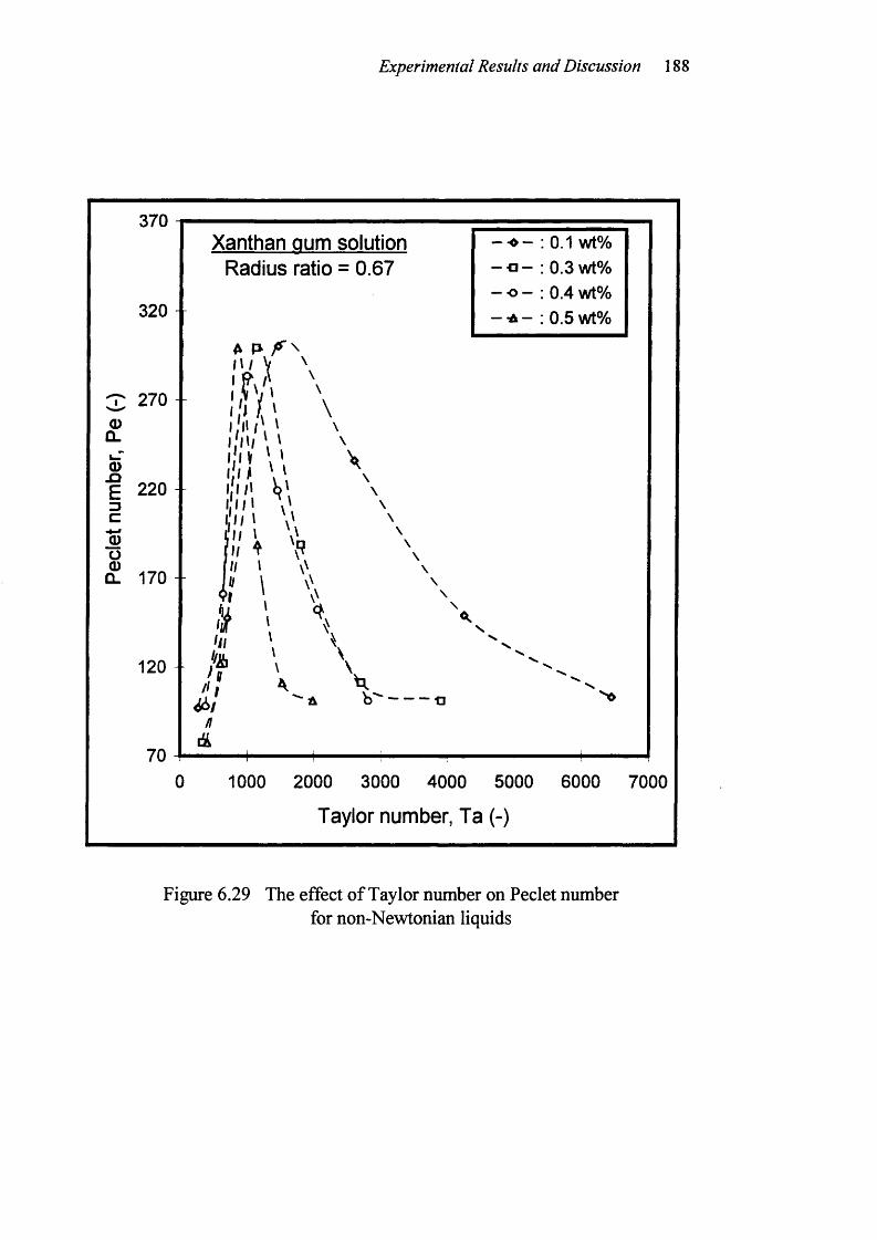
Experimental Results and Discussion 18 8
370Xanthan gum solution
Radius ratio = 0.67: 0.1 wt%
0.3 wt% 0.4 wt% 0.5 wt%
1000 2000 3000 4000 5000 6000 7000
Taylor number, Ta {-)
Figure 6.29 The effect o f Taylor number on Peclet numberfor non-Newtonian liquids
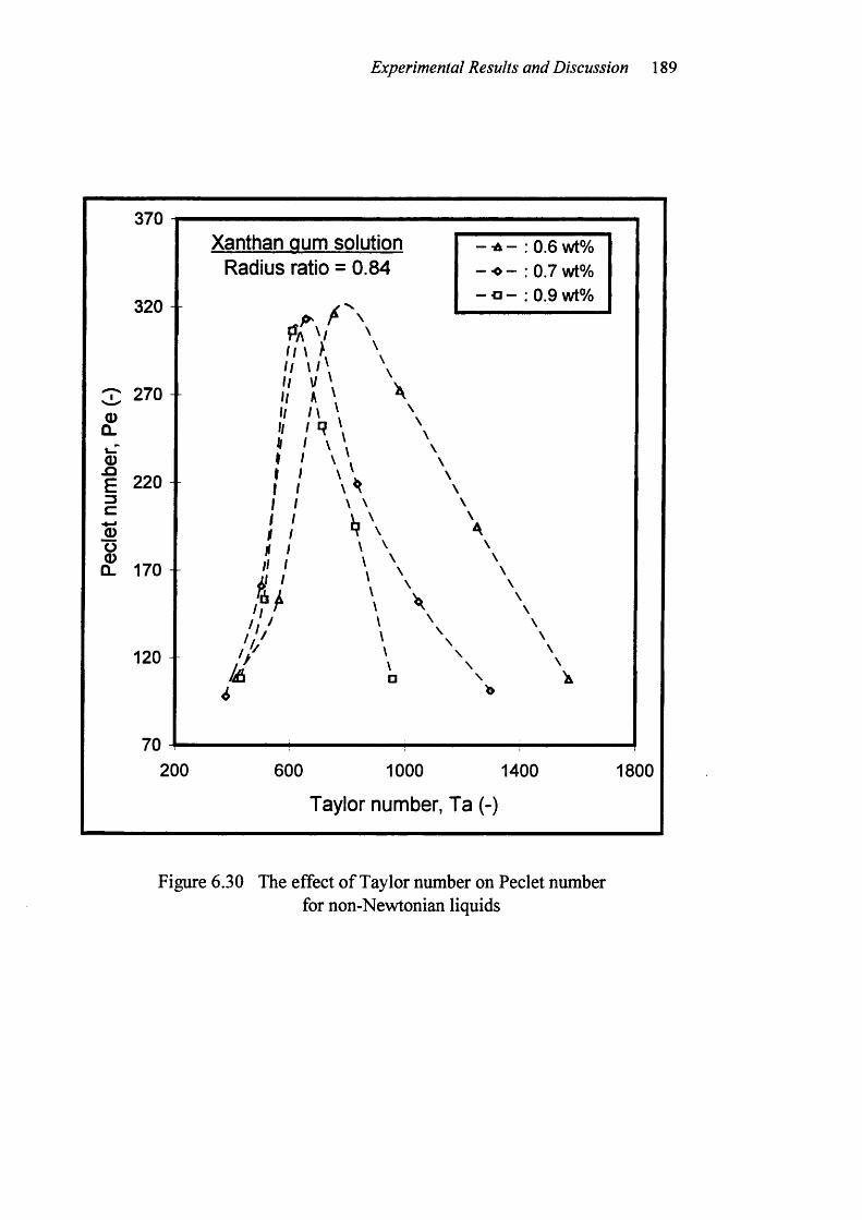
Experimental Results and Discussion 189
370
320 -
2700)Û.
E 2203C0)8Û. 170
120
70200
Xanthan gum solution Radius ratio = 0.84
f:( ' 'n \i\I I V '" * \II i \ \II I R \
— " A —
— ^ —
— O -
0.6 wt% 0.7 wt% 0.9 wt%
I \I II I I I
I I / I f I H I
I I I J I
&■ I '
\\ 4\ \
\ \
\
\□
600 1000 1400
Taylor number, Ta (-)
1800
Figure 6.30 The effect o f Taylor number on Peclet numberfor non-Newtonian liquids
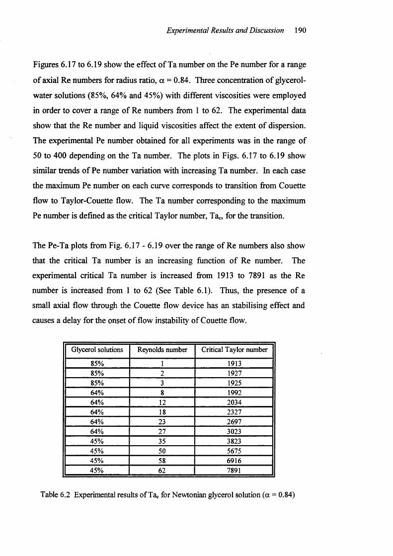
Experimental Results and Discussion 190
Figures 6.17 to 6.19 show the effect o f Ta number on the Pe number for a range
of axial Re numbers for radius ratio, a = 0.84. Three concentration of glycerol-
water solutions (85%, 64% and 45%) with different viscosities were employed
in order to cover a range of Re numbers from 1 to 62. The experimental data
show that the Re number and liquid viscosities affect the extent o f dispersion.
The experimental Pe number obtained for all experiments was in the range of
50 to 400 depending on the Ta number. The plots in Figs. 6.17 to 6.19 show
similar trends o f Pe number variation with increasing Ta number. In each case
the maximum Pe number on each curve corresponds to transition from Couette
flow to Taylor-Couette flow. The Ta number corresponding to the maximum
Pe number is defined as the critical Taylor number, Ta , for the transition.
The Pe-Ta plots from Fig. 6.17 - 6.19 over the range of Re numbers also show
that the critical Ta number is an increasing function o f Re number. The
experimental critical Ta number is increased from 1913 to 7891 as the Re
number is increased from 1 to 62 (See Table 6.1). Thus, the presence of a
small axial flow through the Couette flow device has an stabilising effect and
causes a delay for the onset o f flow instability o f Couette flow.
Glycerol solutions Reynolds number Critical Taylor number
85% 1 191385% 2 192785% 3 192564% 8 199264% 12 203464% 18 232764% 23 269764% 27 302345% 35 382345% 50 567545% 58 691645% 62 7891
Table 6.2 Experimental results o f Ta for Newtonian glycerol solution (a = 0.84)
Experimental Results and Discussion 191
Figures 6.20 to 6.22 show the effect o f Ta number on the Pe number for Re
numbers between 1 and 69 and a radius ratio, a = 0.67. Similar observations
are made from these plots, that is the critical Ta number increases as the axial
Re number increases. The experimental data revealed that the radius ratio also
affected the extent o f dispersion. Table 6.3 shows the critical Taylor number
for a range of Re numbers. By comparing these results with the Table 6.2 for
radius ratio = 0.84, it is seen that the critical Taylor numbers obtained for
radius ratio = 0.67 are generally higher than those for radius ratio = 0.84. (see
Fig. 6.31)
Glycerol solutions Reynolds number Critical Taylor number
85% 1 231685% 2 233885% 4 241064% 7 250864% 17 283164% 22 339464% 25 353664% 29 397845% 47 631845% 55 823445% 61 928745% 69 12196
Table 6.3 Experimental results o f Tag for Newtonian glycerol solution ( a = 0.67)
Figures 6.18 to 6.19 and Figure 6.22 to 6.23 show the effect of Ta number on
the Pe number for a range of concentrations (0.1 - 0.9 wt%) of CMC and
Xanthan gum solutions respectively. A radius ratio, a = 0.84 and seven
concentrations of non-Newtonian solutions were employed in order to cover a
wide range of rheological behaviour o f the liquid from flow index n = 0.254 to
0.653 as shown on the figures.
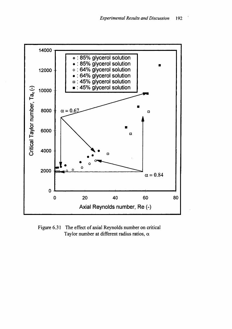
Experimental Results and Discussion 192
14000 185% glycerol solution 85% glycerol solution 64% glycerol solution 64% glycerol solution 45% glycerol solution 45% glycerol solution
12000 -
10000
8000 - a = 0.6
^ 6000
4000
a = 0.84
Axial Reynolds number, Re (-)
Figure 6.31 The effect of axial Reynolds number on criticalTaylor number at different radius ratios, a
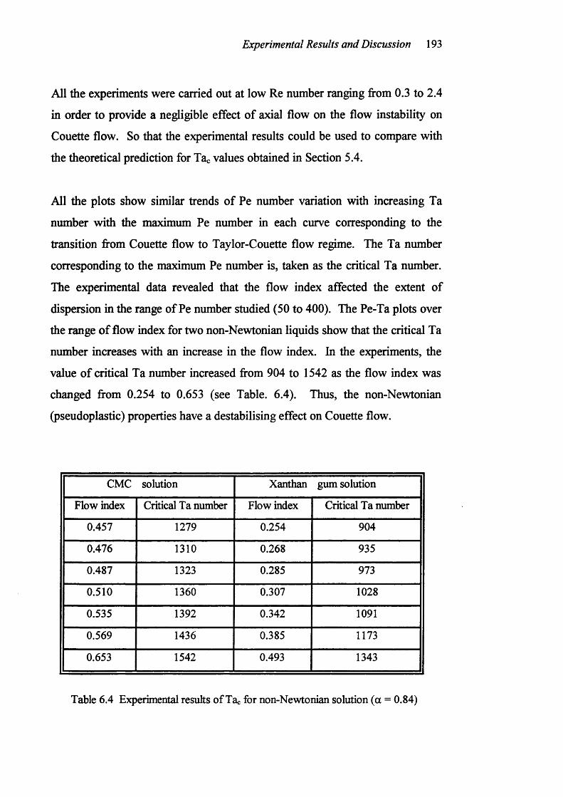
Experimental Results and Discussion 193
All the experiments were carried out at low Re number ranging from 0.3 to 2.4
in order to provide a negligible effect o f axial flow on the flow instability on
Couette flow. So that the experimental results could be used to compare with
the theoretical prediction for Ta values obtained in Section 5.4.
All the plots show similar trends o f Pe number variation with increasing Ta
number with the maximum Pe number in each curve corresponding to the
transition from Couette flow to Taylor-Couette flow regime. The Ta number
corresponding to the maximum Pe number is, taken as the critical Ta number.
The experimental data revealed that the flow index affected the extent of
dispersion in the range of Pe number studied (50 to 400). The Pe-Ta plots over
the range o f flow index for two non-Newtonian liquids show that the critical Ta
number increases with an increase in the flow index. In the experiments, the
value o f critical Ta number increased from 904 to 1542 as the flow index was
changed from 0.254 to 0.653 (see Table. 6.4). Thus, the non-Newtonian
(pseudoplastic) properties have a destabilising effect on Couette flow.
CMC solution Xanthan gum solution
Flow index Critical Ta number Flow index Critical Ta number
0.457 1279 0.254 904
0.476 1310 0.268 935
0.487 1323 0.285 973
0.510 1360 0.307 1028
0.535 1392 0.342 1091
0.569 1436 0.385 1173
0.653 1542 0.493 1343
Table 6.4 Experimental results o f Tac for non-Newtonian solution (a = 0.84)
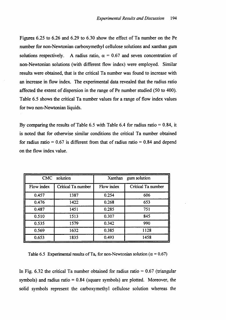
Experimental Results and Discussion 194
Figures 6.25 to 6.26 and 6.29 to 6.30 show the effect o f Ta number on the Pe
number for non-Newtonian carboxymethyl cellulose solutions and xanthan gum
solutions respectively. A radius ratio, a = 0.67 and seven concentration of
non-Newtonian solutions (with different flow index) were employed. Similar
results were obtained, that is the critical Ta number was found to increase with
an increase in flow index. The experimental data revealed that the radius ratio
affected the extent o f dispersion in the range of Pe number studied (50 to 400).
Table 6.5 shows the critical Ta number values for a range of flow index values
for two non-Newtonian liquids.
By comparing the results o f Table 6.5 with Table 6.4 for radius ratio = 0.84, it
is noted that for otherwise similar conditions the critical Ta number obtained
for radius ratio = 0.67 is different from that of radius ratio = 0.84 and depend
on the flow index value.
CMC solution Xanthan gum solution
Flow index Critical Ta number Flow index Critical Ta number
0.457 1387 0.254 6060.476 1422 0.268 6530.487 1451 0.285 7510.510 1513 0.307 8450.535 1579 0.342 9900.569 1632 0.385 11280.653 1835 0.493 1458
Table 6.5 Experimental results of Tac for non-Newtonian solution (a = 0.67)
In Fig. 6.32 the critical Ta number obtained for radius ratio = 0.67 (triangular
symbols) and radius ratio = 0.84 (square symbols) are plotted. Moreover, the
solid symbols represent the carboxymethyl cellulose solution whereas the
Experimental Results and Discussion 195
hollow symbols represent the xanthan gum solutions. It is observed from Fig.
6.32 that the Couette flow is generally destabilised with decreasing flow index,
n. The extent of the reduction in the critical Ta number depends on the flow
index.
Figure 6.32 also shows that when flow index is greater than 0.4, the critical Ta
number obtained for radius ratio = 0.67 is generally higher than that o f radius
ratio = 0.84. This is in agreement with data on the Newtonian liquids (Section
5.2.3). However, it is noted the extent of increase in the critical Ta number is
gradually decreased with decreasing flow index. When flow index is lesser
than 0.4, an adverse effect appeared, that is the critical Ta number obtained for
radius ratio = 0.67 was found to be lower than that of radius ratio = 0.84. It is
suggested that the stability of the Couette flow not only depends on the radius
ratio but also the flow index.
As shown previously in Fig. 5.11 that as the flow index decreases, the radial
variation of shear stress across the annular gap becomes more pronounced and
the shear stress distribution becomes highly hyperbolic. As the gap width
increases, the effect of flow index on the critical Ta number becomes more
prominent and the rate of decrease of critical Ta number with respect to flow
index is faster in the wide gap geometry (radius ratio = 0.67) than that of the
narrow gap geometry (radius ratio = 0.84).
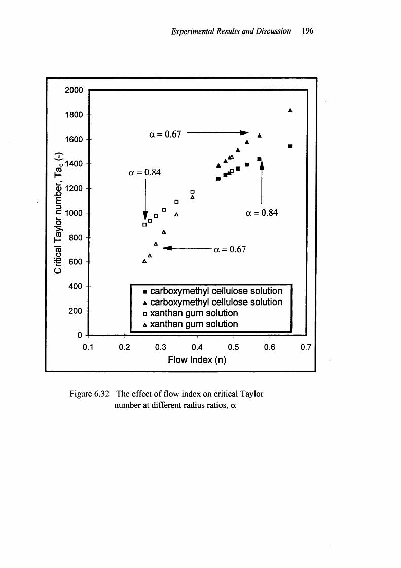
Experimental Results and Discussion 196
2000
1800
1600 -
o1400(Ü
(D 1200Ic 1000o>%^ 800
8g 600 O
400
200 +
0
a = 0.67
a = 0.84
□a = 0.84
a = 0.67
■ carboxymethyl cellulose solution A carboxymethyl cellulose solution □ xanthan gum solution A xanthan gum solution
0.1 0.2 0.3 0.4 0.5 0.6 0.7Flow Index (n)
Figure 6.32 The effect of flow index on critical Taylornumber at different radius ratios, a
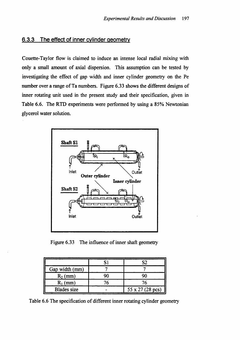
Experimental Results and Discussion 197
6.3.3 The effect of inner cylinder geometry
Couette-Taylor flow is claimed to induce an intense local radial mixing with
only a small amount of axial dispersion. This assumption can be tested by
investigating the effect of gap width and inner cylinder geometry on the Pe
number over a range o f Ta numbers. Figure 6.33 shows the different designs of
inner rotating unit used in the present study and their specification, given in
Table 6.6. The RTD experiments were performed by using a 85% Newtonian
glycerol water solution.
Shaft SI
Inlet \ Outlet
Inner cylinderOuter cylinder
Shaft S2
Inlet Outlet
Figure 6.33 The influence of inner shaft geometry
SI S2Gap width (mm) 7 7
R] (mm) 90 90Ri (mm) 76 76
Blades size - 55 X 27 (28 pcs)
Table 6.6 The specification of different inner rotating cylinder geometry
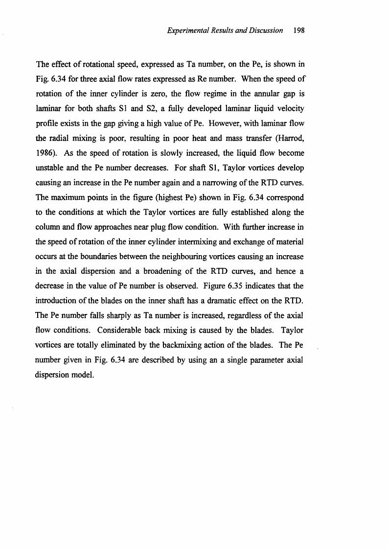
Experimental Results and Discussion 198
The effect o f rotational speed, expressed as Ta number, on the Pe, is shown in
Fig. 6.34 for three axial flow rates expressed as Re number. When the speed o f
rotation o f the inner cylinder is zero, the flow regime in the annular gap is
laminar for both shafts SI and 82, a fully developed laminar liquid velocity
profile exists in the gap giving a high value of Pe. However, with laminar flow
the radial mixing is poor, resulting in poor heat and mass transfer (Harrod,
1986). As the speed of rotation is slowly increased, the liquid flow become
unstable and the Pe number decreases. For shaft 81, Taylor vortices develop
causing an increase in the Pe number again and a narrowing of the RTD curves.
The maximum points in the figure (highest Pe) shown in Fig. 6.34 correspond
to the conditions at which the Taylor vortices are fully established along the
column and flow approaches near plug flow condition. With further increase in
the speed o f rotation of the inner cylinder intermixing and exchange of material
occurs at the boundaries between the neighbouring vortices causing an increase
in the axial dispersion and a broadening of the RTD curves, and hence a
decrease in the value of Pe number is observed. Figure 6.35 indicates that the
introduction of the blades on the inner shaft has a dramatic effect on the RTD.
The Pe number falls sharply as Ta number is increased, regardless of the axial
flow conditions. Considerable back mixing is caused by the blades. Taylor
vortices are totally eliminated by the backmixing action of the blades. The Pe
number given in Fig. 6.34 are described by using an a single parameter axial
dispersion model.
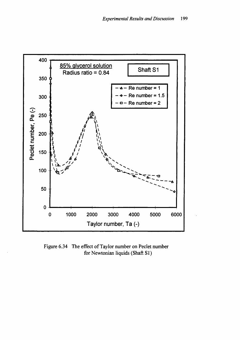
Experimental Results and Discussion 199
400
350 6
300 ^
0) 250 Û.
I 2003C%o 150 0_
100
50
- \ 'I
I4
85% glycerol solution Radius ratio = 0.84 Shaft S1
- -A - Re number = 1- -o - Re number = 1.5 - c - Re number = 2
\
/AI t
I''V
<=-wr--a
1000 2000 3000 4000
Taylor number, Ta (-)
5000 6000
Figure 6.34 The effect of Taylor number on Peclet numberfor Newtonian liquids (Shaft SI)
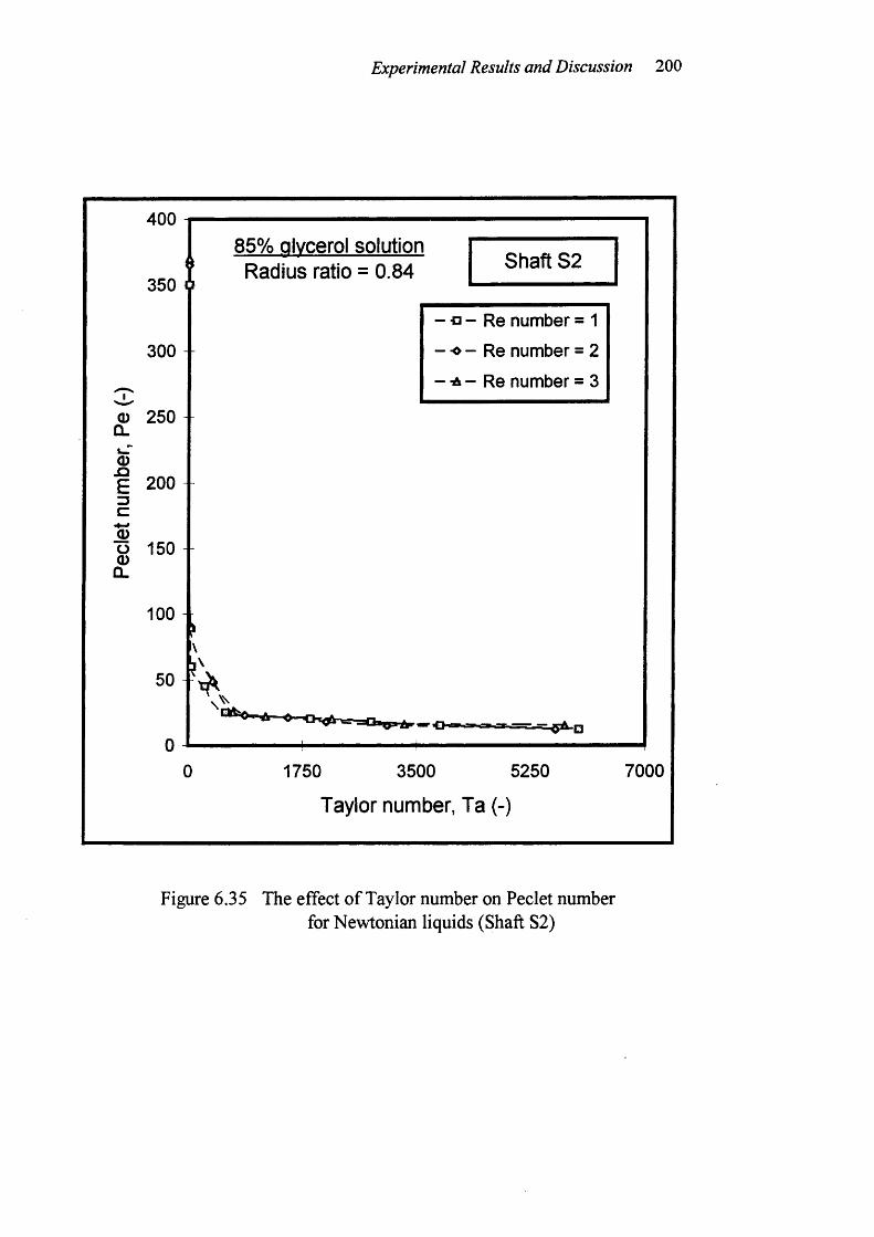
Experimental Results and Discussion 200
400
350
300
Q) 250 CL
OE 2003Co5Ô 150 Û.
100
50
0
85% glycerol solution Radius ratio = 0.84 Shaft 82
A O-
0
- c - Re number = 1
- -o - Re number = 2
- -A - Re number = 3
1750 3500 5250
Taylor number, Ta (-)
7000
Figure 6.35 The effect o f Taylor number on Peclet numberfor Newtonian liquids (Shaft S2)
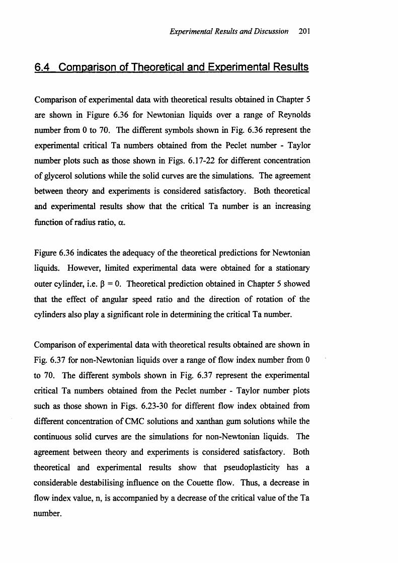
Experimental Results and Discussion 201
6.4 Comparison of Theoretical and Experimental Results
Comparison of experimental data with theoretical results obtained in Chapter 5
are shown in Figure 6.36 for Newtonian liquids over a range of Reynolds
number from 0 to 70. The different symbols shown in Fig. 6.36 represent the
experimental critical Ta numbers obtained from the Peclet number - Taylor
number plots such as those shown in Figs. 6.17-22 for different concentration
of glycerol solutions while the solid curves are the simulations. The agreement
between theory and experiments is considered satisfactory. Both theoretical
and experimental results show that the critical Ta number is an increasing
function of radius ratio, a.
Figure 6.36 indicates the adequacy of the theoretical predictions for Newtonian
liquids. However, limited experimental data were obtained for a stationary
outer cylinder, i.e. P = 0. Theoretical prediction obtained in Chapter 5 showed
that the effect o f angular speed ratio and the direction of rotation of the
cylinders also play a significant role in determining the critical Ta number.
Comparison of experimental data with theoretical results obtained are shown in
Fig. 6.37 for non-Newtonian liquids over a range o f flow index number from 0
to 70. The different symbols shown in Fig. 6.37 represent the experimental
critical Ta numbers obtained from the Peclet number - Taylor number plots
such as those shown in Figs. 6.23-30 for different flow index obtained from
different concentration of CMC solutions and xanthan gum solutions while the
continuous solid curves are the simulations for non-Newtonian liquids. The
agreement between theory and experiments is considered satisfactory. Both
theoretical and experimental results show that pseudoplasticity has a
considerable destabilising influence on the Couette flow. Thus, a decrease in
flow index value, n, is accompanied by a decrease of the critical value of the Ta
number.
Experimental Results and Discussion 202
The theoretical simulations and experimental data in Fig. 6.37 also show that
the effect of flow behaviour index on the critical Ta number as a function o f a
is complex and depends on the value of n. For flow behaviour index, n, less
than 0.4 the critical Ta number increases as a increases, while o f n greater than
0.4 the reverse occurs. This was explained in terms of changes in the stress
distribution within the gap as a function of radial position for different values
of flow behaviour index (see Section 6.3.2).
Experimental Results and Discussion 203
E3CL_o
S*u-o
14000o : 85% glycerol solution♦ : 85% glycerol solution o : 64% glycerol solution# : 64% glycerol solution □ : 45% glycerol solution ■ ; 45% glycerol solution
a = 0.6
12000
a = 0.7
10000 a = 0.
a = 0.9
8000
a = 0.67
6000
4000
2000 a = 0.84
0806020 400
Axial Reynolds number, Re (-)
Figure 6.36 Comparison of theoretical and experimental resultsfor Newtonian liquids
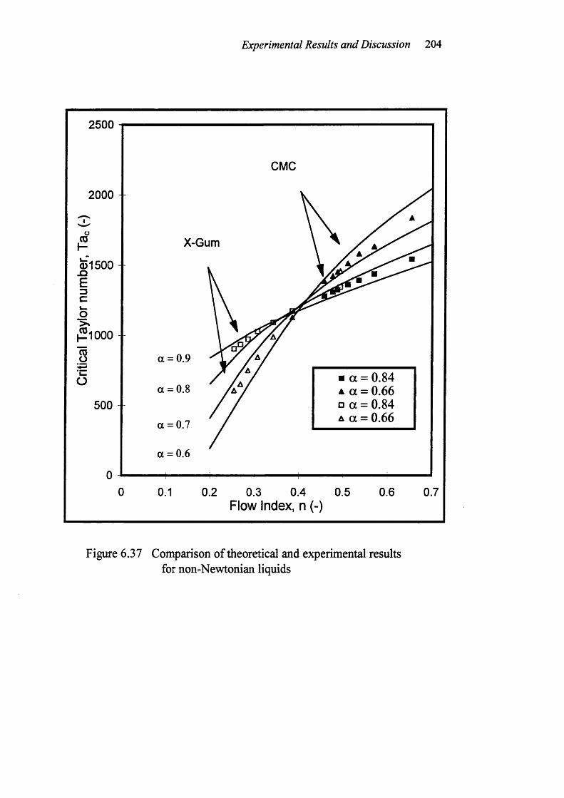
Experimental Results and Discussion 204
2500
CMC
2000
X-Gum
a = 0.9
■ a = 0.84 A a = 0.66 □ a = 0.84 A a = 0.66
a = 0.8
500 -a = 0.7
a = 0.6
0.3 0.4Flow Index, n (-)
0.5 0.6 0.70.2
Figure 6.37 Comparison of theoretical and experimental resultsfor non-Newtonian liquids
Conclusions 205
CHAPTER SEVEN
CONCLUSIONS
7.1 Conclusions
The liquid motion induced between a pair of rotating cylinders with a small
amount of superimposed axial flow has potential applications in many chemical
and biochemical operations. In the present study, the onset o f flow instability
(defined as critical Taylor number) of a range of Newtonian and non-
Newtonian liquids in Couette flow has been considered both theoretically and
experimentally.
In the mathematical analysis, the theoretical study on the flow instability o f a
Newtonian liquid in Couette flow has been extended to include cases o f wide
radius ratio, angular speed ratio and the direction of rotation of the cylinders
with and without axial flow.
The present results indicated that the Galerkin method in conjunction with
simple polynomial expansion functions yielded accurate results for a variety of
flow stability problems. The numerical simulations showed that Couette flow
was stabilised (i.e. critical Ta number increased) due to an increase in the gap
width (radius ratio decreased). For a fixed radius ratio, the critical Ta number
decreased in the case of co-rotating and increased in the case of counter-
rotating of the rotating cylinders as a function o f angular speed ratio. In the
presence of a small amount of axial flow, the critical Ta number was found to
increase with an increase in axial flowrate when radius ratio and angular speed
ratio of the rotating cylinders were held constant.
Conclusions 206
Another important theoretical study of Couette flow concerned the effect of
non-Newtonian behaviour of the liquid on the critical Ta number. The
modified governing flow instability equations including the power law flow
index, n, were solved in a satisfactory manner by using the Galerkin method.
The theoretical results showed that critical Ta number was considerably smaller
than for the corresponding case of Newtonian liquids. It was observed that the
variation in the value of critical Ta number due to the rheological was
significant in all cases and dramatic in some, notably when the flow index was
less than 0.4. Generally, it was found that pseudoplasticity had a destabilising
influence on Couette flow. Thus, a decrease in flow index, n, was
accompanied by a decrease in the critical Ta number. In the ranges of the flow
index, O.I < n < 1, the radius ratio, 0.1 < a < 0.95, and the angular speed ratio,
-0.5 < p < 1, the effect of operating variables on the stability limit was
predicted to be almost the same for non-Newtonian liquids as for Newtonian
ones.
The present work was concerned with an experimental and theoretical
investigation o f the flow instability o f a range of Newtonian glycerol solutions
and non-Newtonian liquids in Couette flow. The data on flow instability
(critical Taylor number) were obtained by measuring the residence time
distribution of flow under various conditions of rotational-axial flows. The
operational conditions covered the transition form Couette flow to Couette-
Taylor flow regime.
All the experimental results showed that axial dispersion model could be
successfully used to study the axial mixing of the tracer solution in the main
Couette flow and in turn, the mixing properties o f the liquids could be
quantitatively interpreted in terms of a dimensionless Peclet number. When Pe
approached zero, there existed significant dispersion and hence the flow was
Conclusions 207
mixed flow. When Pe approached infinity, the dispersion was negligible and
hence the flow was near plug flow.
The experimental results indicated that Pe number was dependent upon the
rotational speed o f cylinders, axial Re number and the rheological properties of
the liquid medium with little dependence on the radius ratio. The effect of
rotational speed, expressed as Ta number, on the Pe number, indicated that
when the speed o f rotation of the inner cylinder was zero, the flow regime in
the annular gap was laminar giving a high value o f Pe number. As the speed of
rotation was slowly increased, the Pe number decreased. Formation o f Taylor
vortices caused an increase in the Pe number again. With further increased in
the speed o f rotation, a decrease of Pe number. A typical complete Pe number -
Ta number plot covering the transition from Couette flow to Taylor-Couette
was shown in Fig. 6.34. The variation in Pe number as a function of rotational
speed was successfully described qualitatively in terms of changes in flow
structure within the annular region and quantitatively by comparing the
experimental results with theoretical simulations.
In the present study, the critical Ta number was defined by the peak in the plot
of Pe number versus Ta number for a given axial Re number. Results showed
that the value of critical Ta number was an increasing function of gap width
and the Re number for both Newtonian and non-Newtonian liquids. The
critical Ta number was also reported for a wide range of non-Newtonian liquids
whose rheological properties were expressed in term of a power law flow
index, n. The results showed that decrease in the value of flow index caused a
decrease in the critical Ta number. This indicated that for otherwise similar
conditions the flow of a non-Newtonian, shear thinning, liquid in the gap of a
pair of counter rotating cylinders was significantly less stable compared with a
Newtonian liquid. Theoretical simulations and experimental observations of
Conclusions 208
flow instability with and without superimposed axial flow were in good
agreement.
7.2 Recommendations for further work
In the present study, theoretical equations were developed and were
numerically solved for the onset o f flow instability in Couette flow. The
formulation was applicable to flow of both Newtonian and non-Newtonian
liquids. The numerical simulations were presented in terms of the critical Ta
number as a function of four dimensionless groups affecting it, i.e. the Re
number, the dimensionless radius ratio, and the angular speed ratio of
concentric rotating cylinder and the power law flow index o f the liquid
properties.
The experimental observations based on the RTD data and the associated
numerical simulations presented have important implications for the design and
operation of equipment in which Taylor-Couette flow was used to enhance
transport and reaction processes. These operations should be part o f any future
practical studies o f Taylor-Couette flow.
The present theoretical model is limited to power-law shear thinning liquids
only. Many industrially important liquids have viscoelastic and time-dependent
properties. The formulation of the theory described in the present study should
serve as a basis for future studies rheologically more complex liquids in
Couette system.
Conclusions 209
Experimentally, the design o f the equipment used in the present study was such
that only the inner cylinder could be rotated. Any fiiture research in this area
should modify the apparatus to allow independent rotation o f the outer
cylinder. The data obtained from experiments with this modified device could
then be compared with theoretical simulations (Fig. 5.6) to provide further
confirmation o f the modelling presented in this thesis.
The theoretical analysis presented in this study demonstrates the mathematical
complexity of the problem even for the simple case two coaxial cylinder
geometry. As far as the author is aware no theoretical solution exist for the
case of a rotating blade in the shell. It may be possible to obtain reasonable
simulations of the flow in such a case by using a computational fluid dynamics
(CFD) and it is recommended that this should form part of any further work in
this area.
Nomenclature 2 10
NOMENCLATURE
Notations
A = Constant (s-')a = Wave number (-)
an = Coefficient of trial function (-)
B = Constant (s')b = Gap width of the rotating cylinder (m)
bn = Coefficient o f trial function (-)
Ce = Concentration (kg/m^)
Ct = Concentration (kg/m^)
D = Axial dispersion coefficient (m" s ')
D = Differential operator (-)
D = Dimensionless differential operator (-)
D* = Differential operator (-)
D* = Dimensionless differential operator (-)
= Differential operator (-)
= Dimensionless differential operator (-)
F = Dimensionless axial flow velocity (-)
Fg = Geometrical factor in Eq. [2.4] (-)
K = Consistency index (Pa s')
K2 = Parameter defined in Eq. [3.75] (-)
L = Distance between two measuring points (m)
M = Dimensionless angular speed, (-)
N = Number of term used in the trial
and weighting functions (-)
Nomenclature 211
N
n
P
P
Pe
Q
r
Ri
R2
Ray
Re
Ro
s
t
Ta
Tac
u
Um
Un
V
V(r)
Vm
Vn
W
W
W(r)
X
z
= Rotational speed of cylinder
= Flow index
= Dimensionless viscosity
= Pressure
= Peclet number [= WLD" ]
= Dimensionless parameter based on the magnetic
and electric properties in Eq. [2.2]
= Radial coordinate
= Radii of inner cylinders
= Radii of outer cylinders
= Rayleigh number
= Axial Reynolds number [= W(R2 - Ri )v“ ]
= Mean radius
= Growth rate of disturbances
= Time
= Taylor number [=-4Q o(R 2 - Ri)Av"^ ]
= Critical Taylor number
= Radial velocity component
= Weighting function
= Trial fimction
= Tangential velocity component
= Tangential velocity
= Weighting fimction
= Trial function
= Axial flow velocity
= Average axial flow velocity
= Axial velocity component
= Transformed dimensionless radial coordinate
= Axial coordinate
(rps)
(-)
(-)
(Pa)
(-)
(-)(m)
(m)
(m)
(-)
(-)
(m)
(-)
(s)
(-)
(-)(m s'')
(-)
(-)(m $■')
(m s'')
(-)
(-)(m s'')
(m s'')
(m s'')
(-)(m)
Nomenclature 212
Greeks Symbols
a = Radius ratio, (-)
P = Angular speed ratio, (-)
ÿ = Shear rate (s')
Ô = Parameter defined in Eq. [3.25] (-)
8 = Weighting function (-)
r = Dimensionless constant. (-)
n = Apparent viscosity (kgm‘ s"
Tim = Mean apparent viscosity (kgm‘ s'
X = Dimensionless wave number (m-‘)
= Viscosity o f the working liquid (kgm" s"
ILL» = Upper limit viscosity of the working liquid (kgm' s'
14 = Apparent viscosity o f the working liquid (kgm‘ s'
Ho = Zero-shear viscosity of the working liquid (kgm' s"
Hp = Plastic viscosity of the working liquid (kgm'
V = Kinematics viscosity of the working liquid (kgm' s‘^
0 = Dimensionless time (-)
0 = Tangential coordinate (m)
CT = Dimensionless growth rate (-)
cr' = Variance (s') •
= Dimensionless variance (-)
Aae^ = Dimensionless variance difference (-)
T = Shear stress (Pa)
Xy = Yield stress (Pa)
Û) = Angular velocity given by Eq. (16) (rad')
Q(r) = Angular velocity (rad')
Ü1 = Angular velocities o f inner cylinders (rad')
Nomenclature 213
Q2 = Angular velocities of outer cylinders (rad‘ )
Qo = Average angular velocity (rad' )
= Dimensionless variable (-)
v|/(r) = Perturbation on the magnetic field in Eq. [2.2] (-)
Superscripts and Subscripts
= Average value
' = Perturbed quantity
~ = Eigenfunction
= Dimensionless eigenfunction
c = Critical value
Abbreviation
CMC = Carboxymethyl cellulose
Pe = Peclet number
Re = Reynolds number
RTD = Residence time distribution
Ta = Taylor number
References 214
REFERENCES
Abdallah, Y.A.G. and Coney, J.E.R. 1988. Adiabatic and diabatic flow studies
by shear stress measurements in annuli with inner cylinder rotation, J.
Fluid Engng, Trans. ASME, 110(12), 399-405.
Andereck, C.D., Dickman, R. and Swinney, H.L. 1983. New flows in a circular
Couette system with co-rotating cylinders, Phys. Fluids, 26, 1395-1401.
Andereck, D., Liu, S. S. and Swinney, H. L. 1986. Flow regimes in a circular
Couette system with independently rotating cylinders, J. Fluid Mech.,
164, 155-183.
Astill, K.N. 1964. Studies o f the developing flow between concentric cylinders
with the inner cylinder rotating, J. Heat Transfer, Trans. ASME, C86,
383-392.
Beaudoin, G. and Jaffrin, M.Y. 1989. Plasma filtration in Couette flow
membrane devices, Artif. Organs, 13(1), 43-51.
Becker and Kaye, J. 1962. The influence of a radial temperature gradient on the
instability o f fluid flow in an annulus with an inner rotating cylinder, J.
Heat Transfer, Trans. ASME, C84, 106-111.
Benjamin, T.B. 1978a. Bifurcation phenomena in steady flow of a viscous
fluid. I. Theory, Proc. R. Soc. London, A359, 1-26.
Benjamin, T.B. 1978b. Bifurcation phenomena in steady flows o f a viscous
fluid. II. Experiments, Proc. R. Soc. London, A 359, 27-43.
Bird, R.B., Stewart, W.E. and Li^tfoot, E.N. 1960. Transport phenomena.
Chapter III, John Wiley and Sons, Singapore.
Burkhalter, J. E. and Koschmieder, E. L. 1973. Steady supercritical Taylor
vortex flow, J. Fluid Mech., 58(3), 547-560.
Burkhalter, I.E. and Koschmieder, E.L. 1974. Steady supercritical Taylor
vortex after sudden starts, Phys. Fluids, 17(11), 1929-1935.
References 215
Chandrasekhar, S. 1953. The stability of viscous flow between rotating
cylinders in the presence of a magnetic field, Proc. Roy. Soc. A216,
293-309.
Chandrasekhar, S. 1954. The stability of viscous flow between rotating
cylinders, Mathematika, 1, 5-13.
Chandrasekhar, S. 1958. The stability o f viscous flow between rotating
cylinders in the presence of a magnetic field, Proc. Roy. Soc. A 246,
301-311.
Chandrasekhar, S. 1961. Hydrodynamic and Hydromagnetic Stability. Chapter
VII, Oxford, Clarendon Press.
Chandrasekhar, S. 1962. The stability of spiral flow between rotating cylinders,
Proc. Roy. Soc., A 265, 188-197.
Chandrasekhar, S. and Elbert, D. 1962. The stability o f viscous flow between
rotating cylinders - II, Proc. Roy. Soc., A 268, 145-152.
Chung, K.C. and Astill, K.N. 1977. Hydrodynamic instability of viscous flow
between rotating coaxial cylinders with fully developed axial flow, J.
Fluid Mech., 81(4), 641-655.
Cohen, S. and Maron, D. M. 1983. Experimental and theoretical study of a
rotating annular flow reactor, Chem. Engng J., 27, 87-97.
Coles, D. 1965. Transition in circular Couette flow, J. Fluid Mech., 21(3), 385-
425.
Coney, J.E.R. and Simmers, D.A. 1979. A study of fully-developed, laminar,
axial flow and Taylor vortex flow by means of shear stress
measurements, J. Mech. Engng Sci., 21(1), 19-24.
Croockewit, P., Honig, C. C. and Kramers, H. 1955. Longitudinal diffusion in
liquid flow throu^ an annulus between a stationary outer cylinder and a
rotating inner cylinder, Chem. Engng Sci., 4, 111-118.
Danckwerts, P. V. 1953. Continuous flow systems - Distribution of Residence
times, Chem. Eng. Sci., 2(1), 1-13.
References 216
Di Prima, C. and Pridor, A. 1979. The stability o f viscous flow between
rotating concentric cylinders with an axial flow, Proc. Roy. Soc.
London, Ser. A 246, 312-325.
Di Prima, R.C. 1955. Application of the Galerkin method to problems in
hydrodynamic stability, Quart. Applied Mathematics, 13, 55-62.
Di Prima, R.C. 1960. The stability o f a viscous flow between rotating cylinders
with an axial flow, J. Fluid Mech., 9, 621-631.
Di Prima, R.C. and Swinney, H.L. 1981. Instabilities and transition in flow
between concentric rotating cylinders. In Hydrodynamic Instabilities
and the Transition to Turbulence. Eds. Swinney and Gollub, Springer,
Berlin, Heidelberg, New York, 139-180.
Donnelly, R. J. 1991. Taylor-Couette flow: The early days. Physics today, 11,
32-39.
Elliott, L. 1973. Stability o f a viscous fluid between rotating cylinders with
axial flow and pressure gradient round the cylinders, Phys. Fluids, 16,
577-580.
Enokida, Y., Nakata, K. and Suzuki, A. 1989. Axial turbulent diffusion in fluid
between rotating coaxial cylinders, A.I.Ch.E. J., 35, 1211-1214.
Fenstermacher, P.R., Swinney, H.L. and Gollub, J.P. 1979. Dynamical
instabilities and the transition to chaotic Taylor vortex flow, J. Fluid
Mech., 94, 103-128.
Fletcher, C.A.J., 1984. Computational Galerkin Methods. Springer series in
computational physics. Chap I, Springer-Verlag, New York.
Giesekus, J. 1972. On instabilities in Poiseuille and Couette flows of
viscoelastic fluids. Prog. Heat Mass Transfer, 5, 187-193.
Ginn, R.F. and Denn, M.M. 1969. Rotational Stability in Viscoelastic liquids:
Theory, A.I.Ch.E. J., 15, 450-454.
Goldstein, S. 1937. The stability of viscous fluid flow between rotating
cylinders, Proc. Camb. Phil. Soc., 33,41-61.
References 217
Gorman, M. and Swinney, H.L. 1982. Spatial and temporal characteristics of
modulated waves in the circular Couette system, J. Fluid Mech., 117,
123-142.
Graebel, W.P. 1961. Stability of a Stokesian fluid in Couette flow, Phys.
Fluids, 4, 362-368.
Gu, Z.H. and Fahidy, T.Z. 1986. The effect o f geometric parameters on the
structure of combined axial and Taylor-vortex flow, Can. J. Chem. Eng.,
64, 185-189.
Gu, Z.H. and Fahidy, T.Z., 1985. Visualization of flow patterns in axial flow
between horizontal coaxial rotating cylinders. Can. J. Chem. Eng., 63,
14-21.
Guihard, L., Coeuret, F., Legrand, J., Fahidy, T.Z. and Gu, Z.H. 1989.
Circumferential mixing in the Taylor-Couette reactor, I.Chem.E. Symp.
Ser., 112, 105-117.
Harris D.L. and Reid, W.H. 1964. On the stability of viscous flow between
rotating cylinders. Part 2 Numerical analysis, J. Fluid Mech., 20, 95-
101.
Harrod, M. 1986. Scraped Surface Heat Exchangers - A literature survey of
flow patterns, mixing effects, residence time distribution, heat transfer
and power requirements, J. Food Process Eng., 9, 1-62.
Hasoon, M.A. and Martin, B.W. 1977. The stability of viscous axial flow in an
annulus with a rotating inner cylinder, Proc. Roy. Soc. London, A 382,
351-380.
Hoare, M., Narendranathan, T. J., Flint, J.R., Heywood-Waddington, D., Bell,
D.J. and Dunnill, P. 1982. Disruption of protein precipitates during
shear in Couette flow and in pumps, I & EC Fundamentals, 21(4), 402-
406.
Hughes, T.H. and Reid, W.H. 1968. The stability of spiral flow between
rotating cylinders, Phil. Trans. R. Soc. Lond., A 263, 57-91.
References 218
Kataoka, K. 1986. Taylor vortices and instabilities in circular Couette flow. In
Encyclopedia o f Fluid Mechanics, Vol. 1, 236-274, N.P. Cheremisinoff,
Gulf Publ., Houston.
Kataoka, K. and Takigawa, T. 1981. Intermixing over cell boundary between
Taylor vortices, A.I.Ch.E.J., 27(3), 504-508.
Kataoka, K., Doi, H. and Komai, T. 1977. Heat/mass transfer in Taylor vortex
flows with constant axial flow rates. Int. J. Heat Transfer, 20, 57-63.
Kataoka, K., Doi, H., Hongo, T. and Futagawa, M. 1975. Ideal plug-flow
properties o f Taylor vortex flow, J. Chem. Engng Jap., 8(6), 472-476.
Kaye, J. and Elgar, E C. 1958. Modes of adiabatic and diabatic fluid flow in an
annulus with an inner rotating cylinder, Trans. ASME., 80(4), 753-765.
Kirk-Othmer, 1979. Encyclopedia o f chemical technology, (3rd ed.) 12, John
Wiley and Sons., USA, 45-66.
Kirk-Othmer. 1979. Encyclopedia of chemical technology, (3rd ed.) 5, John
Wiley and Sons., USA, 143-163.
Koschmieder, E.L. 1979. Turbulent Taylor vortex flow, J. Fluid Mech., 93,
515-527.
Koschmieder, E.L. 1993. Taylor vortex Flow, In Bénard Cells and Taylor
Vortices, Part II, Cambridge University Press, USA.
Krueger, E.K. and Di Prima, R.C. 1964. The stability of a viscous fluid
between rotating cylinders with an axial flow, J. Fluid Mech., 19, 528-
538.
Kurzweg, U.H. 1963. The stability of Couette flow in the presence of an axial
magnetic field, J. Fluid Mech., 17, 52-60.
Larson, R.G., Shaqfeh, E.S.G. and Muller, S.J. 1990. A purely elastic
instability in Taylor-Couette flow, J. Fluid Mech., 218, 573-600.
Lathrop, D.P., Fineberg, J. and Swinney, H.L. 1992. Turbulent flow between
concentric rotating cylinders at large Reynolds number, Phys. Rev. Lett.,
68(10), 1515-1525.
References 219
Legrand, L. and Coeuret, F. 1986. Circumferential mixing in one-phase and
two-phase Taylor vortex flows, Chem. Eng. Sci., 41(1), 47-53.
Levenspiel, O. 1972. Chemical reaction Engineering, 2nd ed.. Chapter IX, J.
Wiley, New York.
Lewis, J.W. 1928. An experimental study of the motion o f a viscous liquid
contained between two coaxial cylinders, Proc. Roy. Soc. London, A
117, 388-406.
Meksyn, D. 1961. New methods in laminar boundary-layer theory. Chapter
XXIII & XXIV, London: Pergamon Press, New York.
Moore, C.M.V. and Cooney, C.L. 1995. Axial dispersion in Taylor-Couette
flow device, A.I.Ch.E.J., 41, 723-727.
Ng, S. and Turner, E.R. 1982. On the linear stability o f spiral flow between
rotating cylinders, Proc. R. Soc. Lond., A 382, 83-102.
Pfitzer, H. and Beer, H. 1992. Heat transfer in an annulus between
independently rotating tubes with turbulent axial flow. Int. J. Heat Mass
Transfer, 35(3), 623-633.
Pudjiono, P.I. and Tavare, N.S. 1993. Residence time distribution analysis
from a continuous Couette flow device around critical Taylor number,
Can. J. Chem. Engng, 71, 312-318.
Pudjiono, P.I., Tavare, N.S., Garside, J. and Nigam, K.D.P. 1992. Residence
time distribution from a continuous Couette flow device, Chem. Engng
J., 48, 101-110.
Rayleigh, O.M. 1916. On the dynamics of revolving fluids, Proc. Roy. Soc
London, A 93, 148-154.
Roberts, P.H. 1965. Appendix in experiments on the stability of viscous flow
between rotating cylinders. VI. Finite-amplitude experiments, Proc.
Roy. Soc. London, A 283, 531-556.
Rosant, J., Legrand, J., Rey, C. and Benmerzouka, A. 1994. Separated two-
phase flow in a rotating annulus: application to the extraction of liquid
phase, Chem. Engng Sci., 49(11), 1769-1781.
References 220
Rushton, A. and Zhang, G.S. 1988. Rotary microporous filtration,
Desalination, 70, 379-394.
Sinevic, V., Kuboi, R. and Nienow, A.W. 1986. Power numbers, Taylor
numbers and Taylor vortices in viscous Newtonian and non-Newtonian
fluids, Chem. Eng. Sci. 41, 2915-2923.
Snyder, A. 1970. Waveforms in rotating Couette flow. Intern. J. Nonlinear
Mech., 5, 659-685.
Snyder, H.A. 1969a. Change in waveform and mean flow associated with
wavelength variations in rotating Couette flow. Part 1, J. Fluid Mech.
35, 337-352.
Snyder, H.A. 1969b. Wave number selection at finite amplitude in rotating
Couette flow, J. Fluid Mech., 35, 273-298.
Soundalgekar, V.M., Ali, M.A. and Takhar, H.S. 1994. Hydromagnetic
stability o f dissipative Couette flow: wide-gap problem. Int. J. Energy
Res., 18, 689-695.
Sparrow, E.M., Munro, W.D. and Jonsson, V.K. 1964. Instability of the flow
between rotating cylinders: the wide gap problem, J. Fluid Mech., 20(1),
35-46.
Stuart, J.T. 1986. Taylor-vortex flow: a dynamical system, SIAM Rev., 28(3),
315-342.
Sun, Z.S. and Denn, M.M. 1972. Stability of Rotational Couette flow of
polymer solutions, A.I.Ch.E.J., 18, 1010-1015.
Takeuchi, D.I and Jankowski, D.F. 1981. A numerical and experimental
investigation o f the stability of spiral Poiseuille flow, J. Fluid Mech.,
102, 101-126.
Tam, W.Y. and Swinney, H.L. 1987. Mass transport in turbulent Couette-
Taylor flow, Phys. Rev. A36, 1374-1381.
Taylor, G.I. 1923. Stability of a viscous fluid contained between two rotating
cylinders, Phil. Trans., A 223, 289-343.
References 221
Tobler, W. 1982. Dynamic filtration: principle and application o f shear
filtration in an annular gap, Filtr. Sep., 19, 329-332.
Walden, R.W. and Donnelly, R.J. 1979. Re-emergent order of chaotic circular
Couette flow, Phys. Rev. Lett., 42(5), 301-304.
Walowit, J., Tsao, S. and Di Prima, R.C. 1964. Stability of flow between
arbitrarily spaced concentric cylindrical surfaces including the effect o f
a radial temperature gradient, Trans. ASME, 12, 585-593.
Wamecke, H., Pruss, J. and Langemann, H. 1985. On a mathematical model
for loop reactors - I. Residence time distribution, moments and
eigenvalues, Chem. Engng Sci., 40(12), 2321-2326.
Wen, Y. and Fan, L.T. 1975. Models for flow systems and chemical reactors,
Marcel Dekker, New York.
Wey, J.S. and Estrin, J. 1973. Modelling the batch crystallization process: the
ice-brine system, Ind. Eng. Chem. Process Des. Dev., 12(3), 236-246.
Appendix One 222
APPENDIX ONE
GALERKIN METHOD
The Galerkin method has been used to solve problems in structural mechanics,
dynamics, fluid flow, hydrodynamic stability, heat and mass transfer, acoustics,
microwave theory, neutron transport, etc. Problems governed by ordinary
differential equations, partial differential equations, and integral equations have
been investigated via the Galerkin formulation. Steady, unsteady, and
eigenvalue problems have proved to be equally amenable to the Galerkin
treatment. Essentially, any problem for which governing equations can be
written down is a candidate for a Galerkin method (Fletcher, 1984).
Basically, it is a method for finding the approximate solution of an eigenvalue
or eigenelement problems in the form of a linear combination of the elements
of given linear independent system. In engineering practice the exact solution
can only be known in a few simple cases and it is therefore important to see
how the solution behaves when one introduces an approximation. By
approximating the function u given by Eq. [A 1.1] as:
u = a i (})i+tt2 (|>2 +... [ A l . l ]
where Oi are unknown coefficients and the (|)i is a set of linearly independent
functions which are known. Oj are generalized coefficients although in some
cases they can be associated with nodal values of the variable under
consideration. In general fluid flow engineering problems, it is preferable to
use nodal values as they provide a clear physical meaning (such as boundary
conditions) via the finite elements, finite differences or the boundary element
method. In such cases the approximation for u can be written as:
Appendix One 223
U = U1 (j)l + U2 <j)2+... [A1.2]
u = ^uj(j)j [A1.3]j=i
where <t>j is a set o f linearly independent functions which are sometimes called
interpolation functions, uj are the nodal values of the field variable and its
derivative (which are generally any variable with physical meaning directly
related to u).
Introducing the approximation for u into the governing differential equation, an
expression is obtained which is no longer identically satisfied except for the
case where Eqs. [A l.l] or [A 1.2] can represent the exact solution. This
produces an error or residual function in the domain or the boundary due to the
inadequacy of the above equations. The error function in the domain is called
R. The numerical methods are used in controlling the value of R as small as
possible by setting its residual equal to zero for various values of the weighting
functions, i|/j, such that
jRv|/jdQ = 0 in n j = l ,2, . . . ,N [A1.4]n
where Q is the domain condition. These functions have to be linearly
independent. In the case of the Galerkin method the weighting functions are
the same as the approximating functions, i.e. (|)j = if/j; hence Eq.[A1.4] becomes:
fR<tijdQ = 0 j = l , 2 , . . . , N [A1.5]
Equation [A 1.5] will produce a system of algebraic equations from which the
unknown values o f Oi or Ui coefficients of u (in Eqs. [Al. l] or [A1.2]) can be
obtained. The approximation can always be improved by increasing the
number of N functions used, where N is the number of terms in the
approximate solution equal to the number of weighting functions required.
Appendix Two 224
APPENDIX TWO
MATHEMATICA PROGRAM FOR FLOW
INSTABILITY OF NEWTONIAN LIQUIDS
IN COUETTE FLOW
" I N P U T THE S YS TEM GEOMETRY & P R O P E R T I E S " ;" n = m a t r i x s i z e r e q u i r e d" n b a = n u m b e r o f d i m e n s i o n l e s s w a v e n u m b e r i n p u t" i a = v a l u e s o f d i m e n s i o n l e s s w a v e n u m b e r i n p u t" n b c = n u m b e r o f d i m e n s i o n l e s s d i s t u r b a n c e g r o w t h
r a t e i n p u t" i c = v a l u e s o f d i m e n s i o n l e s s d i s t u r b a n c e g r o w t h
r a t e i n p u t
C l e a r [ n , n b a , i a , n b c , i c ]
n = 4 ; n b a = 1 5 ;i a = { 2 . 8 , 2 . 9 , 3 . 0 , 3 . 1 , 3 . 1 1 , 3 . 1 2 , 3 . 1 3 , 3 . 1 4 ,
3 . 1 5 , 3 . 1 6 , 3 . 1 7 , 3 . 1 8 , 3 . 1 9 , 3 . 2 , 3 . 3 } ; n b c = 3 ;i c = { l . 1 6 6 , 1 . 1 6 9 , 1 . 1 7 2 } ;
^ ^ ' k ' k ' k ' k ' i r ' i e ' i f ' k ' k ' k ' k - k - k - k ' k - k ' k - k ' k ' i r - k - k - k ' k - k - k - k ' k ' k - k - k ' k - k ' k ' k - k ' k ' k - k ' k ' k ' k - k - k - k - k - k ' k - k - k - k ' k - i e ' k ^ ^ m
" I N P U T THE S YS TEM GEOMETRY & P R O P E R T I E S " ;" a = d i m e n s i o n l e s s w a v e n u m b e r " ;" c = d i m e n s i o n l e s s d i s t u r b a n c e g r o w t h r a t e " ;" r e x = a x i a l R e y n o l d s n u m b e r " ;" r l = r a d i u s o f i n n e r c y l i n d e r " ;" r 2 = r a d i u s o f o u t e r c y l i n d e r " ;" q l = a n g u l a r s p e e d o f i n n e r c y l i n d e r " ;" q 2 = a n g u l a r s p e e d o f o u t e r c y l i n d e r " ;
C l e a r [ a , c , r e x , r l , r 2 , q l , q 2 ]
a [ w _ ] : = i a [ [w] ]c [ m _ ] : = i c [ [m] ]r e x = 1 0 ;r l = 0 . 8 ;r 2 = 1 . 0 ;q l = l ;q 2 = 0 ;
Appendix Two 225
" D E F I N E THE SYS TEM P A R A M E T E R S " ;" h = r a d i u s r a t i o o f c o n c e n t r i c r o t a t i n g c y l i n d e r s" u = a n g u l a r s p e e d r a t i o o f c o n c e n t r i c r o t a t i n g
c y l i n d e r s " s i g = f u n c t i o n o f c , a a n d r e x " ;" k k = f u n c t i o n o f a , s i g , r e x a n d f " ;" s = g e o m e t r i c a l p a r a m e t e r "" e = g e o m e t r i c a l p a r a m e t e r "" y = g e o m e t r i c a l p a r a m e t e r "" g = g e o m e t r i c a l p a r a m e t e r "" f = g e o m e t r i c a l p a r a m e t e r "
C l e a r [ h , u , s i g , k k , s , e , y , g , f ]
h = r l / r 2 ;u = q 2 / q l ;s i g [ m _ , w _ ] : = c [ m ] a [ w ] r e x ;k k [ m _ , w _ ] : = a [ w ] ^ 2 - ( s i g [ m , w ] - a [ w ] r e x f ) I ;s = 2 ( r 2 - r l ) / ( r 2 + r l ) ;e = ( 1 + s x ) ^ ( - 1 ) ;y = ( 1 + s x ) / ( l - s / 2 ) ;g = 2 / ( ( l + u ) ( l - h " 2 ) ) ( ( u - h ^ 2 ) + ( l - u ) y " ( - 2 ) ) ;f = ( ( - 2 ) / ( ( l - h ^ 2 ) + ( ( l + h " 2 ) N [ L o g [ h ] ] ) ) ) ( ( l - h ^ 2 )N [ L o g [ y ] ] +
( h " 2 ) ( y " 2 - l ) N [ L o g [ h ] ] ) ;
" D E F I N E T HE D I F F E R E N T I A L O P E R A T O R ,T R I A L F U N C T I O N & W E I G H T I N G F U N C T I O N " ;
" d = d i f f e r e n t i a l o p e r a t o r " ;" d z = d i f f e r e n t i a l o p e r a t o r " ;" u t = t r i a l f u n c t i o n " ;" v t = t r i a l f u n c t i o n " ;" u w = w e i g h t i n g f u n c t i o n " ;" v w = w e i g h t i n g f u n c t i o n " ;^ ^ ' k - k ' k ' k - k ' k - k ' k ' k ' k - k - k ' i r - i r - k - k ' i c - k ' k ' k - k ' k - k ' k ' k ' k ' k - i e - k ' ^ ' k - k - k - k - i e ' k ' k - k ' k ' k ' k - k ' k - i f ' k ' k - k ' k - k ' k ' k - k - i ^ ' k ^ ^ »
C l e a r [ d , d z , u t , v t , u w , v w ]
d [ i _ ] : = D [ i , x ]d z [ i _ ] : = D [ i , x ] + s e i
u t [ i _ ] : = ( x ^ 2 - l / 4 ) ^ 2 x ^ ( i - l ) v t [ i _ ] : = ( x ^ 2 - l / 4 ) x ^ ( i - l )
u w [ i _ ] : = e ( x ^ 2 - l / 4 ) ^ 2 x ^ ( i - l ) v w [ i ] : = e ( x ^ 2 - l / 4 ) x ^ ( i - l )
Appendix Two 226
" D E F I N E T HE GOVE RNI NG E Q U A T I O N S " ;
C l e a r [ q x a , q x b , q y a , q y b ]
" q x a [ u ] + q x b [ v ] t = = 0 &&" ;" q y a [ v ] + q y b [ u ] = = 0 " ;
q x a [ i _ , m _ , w _ ] : = d [ d z [ u t [ i ] ] ] - k k [ m, w] u t [ i ] - l / a [ w ] ^ 2 ( d [ d z [ d [ d z [ u t [ i ] ] ] ] ] - d [ k k [ m , w ] d z [ u t [ i ] ] ] ) + r e x / ( I a [ w ] ) d [ d [ f ] u t [ i ] ]
q x b [ i _ , m _ , w _ ] : = - g v t [ i ]q y a [ i _ , m _ , w _ ] : = u t [ i ]q y b [ i , m , w ] : = - ( d [ d z [ v t [ i ] ] ] - k k [ m , w ] v t [ i ] )
" A P P L Y G A L E R K I N ME T H O D " ;
C l e a r [ f n , x a , x b , y a , y b ]
f n = F u n c t i o n [ ( i , j } , N I n t e g r a t e [ i j , { x , - 1 / 2 , 1 / 2 } ] ] ;
x a [ i _ , m _ , w _ , j _ ] : = f n [ q x a [ i , m , w ] , u w [ j ] ] x b [ i _ , m _ , w _ , j _ ] : = f n [ q x b [ i , m , w ] , u w [ j ] ] t y a [ i _ , m _ , w _ , j _ ] : = f n [ q y a [ i , m , w ] , v w [ j ] ] y b [ i _ , m _ , w _ , j _ ] : = f n [ q y b [ i , m , w ] , v w [ j ] ]
" A P P L Y M A T R I X S YSTEM TO S OL VE T a y l o r n u m b e r , t " ;
C l e a r [ r x a , r x b , r y a , r y b , m a t ]
r x a [ m _ , w _ , j _ , k _ ] : = T a b l e [ x a [ i , m , w , j ] , { i , 1 , k } ] r x b [ m _ , w _ , j _ , k _ ] : = T a b l e [ x b [ i , m , w , j ] , { i , 1 , k } ] r y a [ m _ , w _ , j _ , k _ ] : = T a b l e [ y a [ i , m , w , j ] , { i , 1 , k } ] r y b [ m _ , w _ , j _ , k _ ] : = T a b l e [ y b [ i , m , w , j ] , { i , 1 , k } ]
m a t [ m _ , w _ , k _ ] : = F l a t t e n [ { T a b l e [ F l a t t e n [ { r x a [ m , w , j , k ] , r x b [ m , w , i , k ] } ] , { ] , l , k } ] .T a b l e [ F l a t t e n [ { r y a [ m , w , j , k ] , r y b [ m , w , j , k ] } ] , { j , 1 , k } ] } , 1 ]
" F ORMAT THE O U T P U T " ;
C l e a r [ s o l s , a n s , o k l , o k 2 , r e s O l ]
Appendix Two 227
s o l s [ m _ , w _ , k _ ] : = S o l v e [ D e t [ m a t [ m, w , k ] ] = = 0 , t ] a n s [ m _ , w _ , k _ ] : = S i m p l i f y [ t / . s o l s [ m , w , k ] ]
o k l [ m _ , w _ ] : = T a b l e [ { { " C - v a l u e = " , c [ m ] } , { " A l p h a = " , a [ w ] } , { " R e y . N o . = " , r e x } , { " R a d i i % = " , h } ,{ " V e l . % = " , u } } ] / / C o l u m n F o r m
o k 2 [ m _ , w _ ] : = T a b l e [ a n s [ m , w , n ] ] / / C o l u m n F o r m
r e s 0 1 = T a b l e [ T a b l e [ T a b l e [ { o k l [ m , w ] , o k 2 [ m , w ] } , { m , 1 , n b c } ] / / T a b l e F o r m , { w , 1 , n b a } ] / / T a b l e F o r m ] / / T a b l e F o r m
T a b l e F o r m [ T a b l e F o r m
C - v a l u e = , 1 . 1 6 6 } 2 1 7 8 . 0 3 - 1 2 . 7 7 0 1 IA l p h a = , 2 . 8 } 3 7 5 3 1 . 1 - 2 8 0 7 . 5 5 IR e y . N o . = , 1 0 } 3 7 5 5 6 7 . - 4 0 6 7 5 . 3 IR a d i i % = , 0 . 8 } 6V e l . % — f 0} 2 . 7 1 0 4 1 1 0 - 2 9 8 4 7 2 . I
C - v a l u e = , 1 . 1 6 9 } 2 1 7 6 . 8 2 - 2 6 . 8 4 1 1 IA l p h a = , 2 . 8 } 3 7 5 2 7 . 8 - 2 9 0 9 . 4 7 IR e y . N o . = , 1 0 } 3 7 5 5 5 0 . - 4 1 1 4 9 . 1 IR a d i i % = , 0 . 8 } 6V e l . % = , 0} 2 . 7 1 0 3 1 0 - 3 0 0 5 2 9 . I
C - v a l u e = , 1 . 1 7 2 } 2 1 7 5 . 5 6 - 4 0 . 9 1 1 7 IA l p h a = , 2 . 8 } 3 7 5 2 4 . 3 - 3 0 1 1 . 3 8 IR e y . N o . = , 1 0 } 3 7 5 5 3 3 . - 4 1 6 2 3 . IR a d i i % =, 0 . 8 } 6V e l . % = , 0} 2 . 7 1 0 1 9 1 0 - 3 0 2 5 8 7 . I
C - v a l u e = , 1 . 1 6 6 } 2 1 5 9 . 2 7 - 5 . 4 1 6 9 7 IA l p h a = f 2 . 9 } 3 5 8 8 5 . 1 - 2 7 3 7 . 8 3 IR e y . N o . = , 1 0 } 3 5 4 2 3 7 . - 3 9 4 9 1 . 4 IR a d i i % = , 0 . 8 } 6V e l . % = f 0} 2 . 5 4 4 0 9 1 0 - 2 8 9 5 0 6 . I
C - v a l u e = , 1 . 1 6 9 } 2 1 5 8 . 1 2 - 1 9 . 5 4 3 2 IA l p h a = , 2 . 9 } 3 5 8 8 1 . 8 - 2 8 3 7 . 8 6 IR e y . N o . = , 1 0 } 3 5 4 2 2 0 . - 3 9 9 5 2 . 6 IR a d i i % = , 0 . 8 } 6V e l . % = , 0 } 2 . 5 4 3 9 8 1 0 - 2 9 1 5 0 2 . I
C - v a l u e = , 1 . 1 7 2 } 2 1 5 6 . 9 3 - 3 3 . 6 6 8 9 IA l p h a = , 2 . 9 } 3 5 8 7 8 . 3 - 2 9 3 7 . 8 9 IR e y . N o . = , 1 0 } 3 5 4 2 0 2 . - 4 0 4 1 3 . 8 IR a d i i % = , 0 . 8 } 6V e l . % = , 0} 2 . 5 4 3 8 7 1 0 - 2 9 3 4 9 9 . I
Appendix Two 228
C - v a l u e = , 1 . 1 6 6 } 2 1 4 7 . 5 1 + 2 . 5 6 1 4 5 IA l p h a = , 3 . } 3 4 4 1 7 . - 2 6 7 3 . 5 9 IR e y . N o . = , 1 0 } 3 3 5 0 3 9 . - 3 8 3 9 4 . 6 IR a d i i % = , 0 . 8 } 6V e l . % = , 0} 2 . 3 9 4 2 2 1 0 - 2 8 1 1 8 8 . I
C - v a l u e = , 1 . 1 6 9 } 2 1 4 6 . 4 3 - 1 1 . 6 4 9 8 IA l p h a = , 3 . } 3 4 4 1 3 . 6 - 2 7 7 1 . 9 4 IR e y . N o . = , 1 0 } 3 3 5 0 2 2 . - 3 8 8 4 4 . 2 IR a d i i % = , 0 . 8 } 6V e l . % — r 0} 2 . 3 9 4 1 1 1 0 - 2 8 3 1 2 9 . I
C - v a l u e = , 1 . 1 7 2 } 2 1 4 5 . 3 - 2 5 . 8 6 0 6 IA l p h a = , 3 . } 3 4 4 1 0 . 2 - 2 8 7 0 . 2 9 IR e y . N o . = , 1 0 } 3 3 5 0 0 5 . - 3 9 2 9 3 . 7 IR a d i i % = , 0 . 8 } 6V e l . % = , 0 } 2 . 3 9 4 1 0 - 2 8 5 0 6 9 . I
C - v a l u e = , 1 . 1 6 6 } 2 1 4 2 . 2 + 1 1 . 1 8 8 8 IA l p h a = , 3 . 1 } 3 3 1 0 4 . 8 - 2 6 1 4 . 2 9 IR e y . N o . = , 1 0 } 3 1 7 7 0 6 . - 3 7 3 7 6 . 7 IR a d i i % = , 0 . 8 } 6V e l . % = , 0} 2 . 2 5 8 7 1 1 0 - 2 7 3 4 5 8 . I
C - v a l u e = , 1 . 1 6 9 } 2 1 4 1 . 1 8 - 3 . 1 3 6 0 4 IA l p h a = f 3 . 1 } 3 3 1 0 1 . 5 - 2 7 1 1 . 1 4 IR e y . N o . = , 1 0 } 3 1 7 6 8 9 . - 3 7 8 1 5 . 5 IR a d i i % = , 0 . 8 } 6V e l . % = , 0} 2 . 2 5 8 6 1 0 - 2 7 5 3 4 6 . I
C - v a l u e = , 1 . 1 7 2 } 2 1 4 0 . 1 2 - 1 7 . 4 6 0 3 IA l p h a = , 3 . 1 } 3 3 0 9 8 . 1 - 2 8 0 7 . 9 9 IR e y . N o . = , 1 0 } 3 1 7 6 7 1 . - 3 8 2 5 4 . 4 IR a d i i % = , 0 . 8 } 6V e l .% — f 0} 2 . 2 5 8 4 9 1 0 - 2 7 7 2 3 4 . I
C - v a l u e = , 1 . 1 6 6 } 2 1 4 2 . 0 1 + 1 2 . 0 8 8 1 IA l p h a = , 3 . 1 1 } 3 2 9 8 1 . 5 - 2 6 0 8 . 6 2 IR e y . N o . = , 1 0 } 3 1 6 0 6 6 . - 3 7 2 7 9 . IR a d i i % = , 0 . 8 } 6V e l . % = , 0} 2 . 2 4 5 8 8 1 0 - 2 7 2 7 1 5 . I
C - v a l u e = , 1 . 1 6 9 } 2 1 4 0 . 9 9 - 2 . 2 4 9 6 I;A l p h a = , 3 . 1 1 } 3 2 9 7 8 . 1 - 2 7 0 5 . 3 3 IR e y . N o . = , 1 0 } 3 1 6 0 4 9 . - 3 7 7 1 6 . 8 IR a d i i % =, 0 . 8 } 6V e l . % = , 0} 2 . 2 4 5 7 7 1 0 - 2 7 4 5 9 8 . I
C - v a l u e = , 1 . 1 7 2 } 2 1 3 9 . 9 4 - 1 6 . 5 8 6 8 IA l p h a —f 3 . 1 1 } 3 2 9 7 4 . 7 - 2 8 0 2 . 0 3 IR e y . N o . = , 1 0 } 3 1 6 0 3 1 . - 3 8 1 5 4 . 6 IR a d i i % =, 0 . 8 } 6V e l . % = , 0} 2 . 2 4 5 6 6 1 0 - 2 7 6 4 8 1 . I

Appendix Two 229
C - v a l u e = , 1 . 1 6 6 } 2 1 4 1 . 8 7 + 1 2 . 9 9 4 2 IA l p h a = , 3 . 1 2 } 3 2 8 5 9 . 5 - 2 6 0 2 . 9 8 IR e y . N o . = , 1 0 } 3 1 4 4 4 2 . - 3 7 1 8 2 . IR a d i i % = , 0 . 8 } 6V e l . % = f 0} 2 . 2 3 3 1 7 1 0 - 2 7 1 9 7 7 . I
C - v a l u e = , 1 . 1 6 9 } 2 1 4 0 . 8 6 - 1 . 3 5 6 6 9 IA l p h a = , 3 . 1 2 } 3 2 8 5 6 . 1 - 2 6 9 9 . 5 5 IR e y . N o . = , 1 0 } 3 1 4 4 2 5 . - 3 7 6 1 8 . 7 IR a d i i % = , 0 . 8 } 6V e l . % = , 0} 2 . 2 3 3 0 6 1 0 - 2 7 3 8 5 5 . I
C - v a l u e = , 1 . 1 7 2 } 2 1 3 9 . 8 2 - 1 5 . 7 0 7 IA l p h a =, 3 . 1 2 } 3 2 8 5 2 . 7 - 2 7 9 6 . 1 2 IR e y . N o . = , 1 0 } 3 1 4 4 0 8 . - 3 8 0 5 5 . 5 IR a d i i % = , 0 . 8 } 6V e l . % = , 0} 2 . 2 3 2 9 5 1 0 - 2 7 5 7 3 3 . I
C - v a l u e = , 1 . 1 6 6 } 2 1 4 1 . 7 9 + 1 3 . 9 0 7 IA l p h a = , 3 . 1 3 } 3 2 7 3 8 . 8 - 2 5 9 7 . 4 IR e y . N o . = , 1 0 } 3 1 2 8 3 4 . - 3 7 0 8 5 . 6 IR a d i i % = , 0 . 8 } 6V e l . % = , 0} 2 . 2 2 0 5 9 1 0 - 2 7 1 2 4 5 . I
C - v a l u e = , 1 . 1 6 9 } 2 1 4 0 . 7 9 - 0 . 4 5 7 2 9 2 IA l p h a = , 3 . 1 3 } 3 2 7 3 5 . 5 - 2 6 9 3 . 8 3 IR e y . N o . = , 1 0 } 3 1 2 8 1 7 . - 3 7 5 2 1 . 4 IR a d i i % = , 0 . 8 } 6V e l . % = , 0} 2 . 2 2 0 4 8 1 0 - 2 7 3 1 1 8 . I
C - v a l u e = , 1 . 1 7 2 } 2 1 3 9 . 7 5 - 1 4 . 8 2 1 IA l p h a = , 3 . 1 3 } 3 2 7 3 2 . - 2 7 9 0 . 2 6 IR e y . N o . = , 1 0 } 3 1 2 8 0 0 . - 3 7 9 5 7 . 1 IR a d i i % = , 0 . 8 } 6V e l . % = , 0} 2 . 2 2 0 3 7 1 0 - 2 7 4 9 9 1 . I
C - v a l u e = , 1 . 1 6 6 } 2 1 4 1 . 7 8 + 1 4 . 8 2 6 6 IA l p h a = , 3 . 1 4 } 3 2 6 1 9 . 4 - 2 5 9 1 . 8 5 IR e y . N o . = , 1 0 } 3 1 1 2 4 2 . - 3 6 9 9 0 . IR a d i i % = , 0 . 8 } 6V e l . % = , 0} 2 . 2 0 8 1 2 1 0 - 2 7 0 5 1 7 . I
C - v a l u e = , 1 . 1 6 9 } 2 1 4 0 . 7 8 + 0 . 4 4 8 6 2 1 IA l p h a —f 3 . 1 4 } 3 2 6 1 6 . 1 - 2 6 8 8 . 1 5 IR e y . N o . = , 1 0 } 3 1 1 2 2 5 . - 3 7 4 2 4 . 7 IR a d i i % = , 0 . 8 } 6V e l . % = , 0} 2 . 2 0 8 0 1 1 0 - 2 7 2 3 8 6 . I
C - v a l u e = , 1 . 1 7 2 } 2 1 3 9 . 7 5 - 1 3 . 9 2 8 8 IA l p h a —f 3 . 1 4 } 3 2 6 1 2 . 7 - 2 7 8 4 . 4 4 IR e y . N o . = , 1 0 } 3 1 1 2 0 8 . - 3 7 8 5 9 . 5 IR a d i i % = , 0 . 8 } 6V e l . % = , 0} 2 . 2 0 7 9 1 0 - 2 7 4 2 5 4 . I
Appendix Two 230
{ C - v a l u e = , 1 . 1 6 6 } 2 1 4 1 . 8 2 + 1 5 . 7 5 3 I{ A l p h a = , 3 . 1 5 } 3 2 5 0 1 . 4 - 2 5 8 6 . 3 5 I( R e y . N o . = , 1 0 } 3 0 9 6 6 6 . - 3 6 8 9 5 . I{ R a d i i % = , 0 . 8 } 6{ V e l . % = , 0 } 2 . 1 9 5 7 8 1 0 - 2 6 9 7 9 5 . I
{ C - v a l u e = , 1 . 1 6 9 } 2 1 4 0 . 8 3 + 1 . 3 6 1 0 7 I{ A l p h a = , 3 . 1 5 } 3 2 4 9 8 . 1 - 2 6 8 2 . 5 1 I{ R e y . N o . = , 1 0 } 3 0 9 6 4 8 . - 3 7 3 2 8 . 8 I{ R a d i i % = , 0 . 8 } 6{ V e l . % = , 0} 2 . 1 9 5 6 7 1 0 - 2 7 1 6 5 8 . I
{ C - v a l u e = , 1 . 1 7 2 } 2 1 3 9 . 8 -- 1 3 . 0 3 0 3 I{ A l p h a = , 3 . 1 5 } 3 2 4 9 4 . 6 - 2 7 7 8 . 6 7 I{ R e y . N o . = , 1 0 } 3 0 9 6 3 1 . - 3 7 7 6 2 . 5 I{ R a d i i % = , 0 . 8 } 6{ V e l . % = , 0 } 2 . 1 9 5 5 6 1 0 - 2 7 3 5 2 2 . I
{ C - v a l u e = , 1 . 1 6 6 } 2 1 4 1 . 9 1 + 1 6 . 6 8 6 2 I{ A l p h a = , 3 . 1 6 } 3 2 3 8 4 . 6 - 2 5 8 0 . 8 9 I{ R e y . N o . = , 1 0 } 3 0 8 1 0 4 . - 3 6 8 0 0 . 8 I{ R a d i i % = , 0 . 8 } 6{ V e l . % = , 0} 2 . 1 8 3 5 5 1 0 - 2 6 9 0 7 8 . I
{ C - v a l u e = , 1 . 1 6 9 } 2 1 4 0 . 9 3 + 2 . 2 8 0 0 8 I{ A l p h a = , 3 . 1 6 } 3 2 3 8 1 . 3 - 2 6 7 6 . 9 2 I{ R e y . N o . = , 1 0 } 3 0 8 0 8 7 . - 3 7 2 3 3 . 5 I{ R a d i i % = , 0 . 8 } 6{ V e l . % = , 0} 2 . 1 8 3 4 4 1 0 - 2 7 0 9 3 7 . I
{ C - v a l u e = , 1 . 1 7 2 } 2 1 3 9 . 9 1 - 1 2 . 1 2 5 5 I{ A l p h a = , 3 . 1 6 } 3 2 3 7 7 . 9 - 2 7 7 2 . 9 5 I{ R e y . N o . = , 1 0 } 3 0 8 0 7 0 . - 3 7 6 6 6 . 3 I{ R a d i i % = , 0 . 8 } 6{ V e l . % = , 0} 2 . 1 8 3 3 3 1 0 - 2 7 2 7 9 5 . I
{ C - v a l u e = , 1 . 1 6 6 } 2 1 4 2 . 0 7 + 1 7 . 6 2 6 3 I{ A l p h a = f 3 . 1 7 } 3 2 2 6 9 . 2 - 2 5 7 5 . 4 7 I{ R e y . N o . = , 1 0 } 3 0 6 5 5 8 . - 3 6 7 0 7 . 2 I{ R a d i i % = , 0 . 8 } 6{ V e l . % 0 } 2 . 1 7 1 4 5 1 0 - 2 6 8 3 6 6 . I
{ C - v a l u e = , 1 . 1 6 9 } 2 1 4 1 . 1 4 3 . 2 0 5 6 8 I{ A l p h a = , 3 . 1 7 } 3 2 2 6 5 . 8 - 2 6 7 1 . 3 7 I{ R e y . N o . = , 1 0 } 3 0 6 5 4 1 . - 3 7 1 3 8 . 9 I{ R a d i i % = , 0 . 8 } 6{ V e l . % = , 0 } 2 . 1 7 1 3 4 1 0 - 2 7 0 2 2 0 . I
{ C - v a l u e = , 1 . 1 7 2 } 2 1 4 0 . 0 8 - 1 1 . 2 1 4 4 I{ A l p h a =, 3 . 1 7 } 3 2 2 6 2 . 4 - 2 7 6 7 . 2 7 I{ R e y . N o . = , 1 0 } 3 0 6 5 2 3 . - 3 7 5 7 0 . 7 I{ R a d i i % = , 0 . 8 } 6{ V e l . % = , 0} 2 . 1 7 1 2 2 1 0 - 2 7 2 0 7 3 . I
Appendix Two 231
{ C - v a l u e = , 1 . 1 6 6 } 2 1 4 2 . 2 8 + 1 8 . 5 7 3 3 I{ A l p h a = , 3 . 1 8 } 3 2 1 5 4 . 9 - 2 5 7 0 . 0 9 I{ R e y . N o . = f 1 0 } 3 0 5 0 2 7 . - 3 6 6 1 4 . 2 I{ R a d i i % = , 0 . 8 } 6{ V e l . % = , 0} 2 . 1 5 9 4 5 1 0 - 2 6 7 6 5 9 . I
{ C - v a l u e = , 1 . 1 6 9 } 2 1 4 1 . 3 2 + 4 . 1 3 7 8 8 I{ A l p h a =, 3 . 1 8 } 3 2 1 5 1 . 6 - 2 6 6 5 . 8 7 I{ R e y . N o . = , 1 0 } 3 0 5 0 1 0 . - 3 7 0 4 5 . I{R a d i i % — f 0 . 8 } 6{ V e l . % = , 0} 2 . 1 5 9 3 4 1 0 - 2 6 9 5 0 8 . I
{ C - v a l u e = , 1 . 1 7 2 } 2 1 4 0 . 3 1 - 1 0 . 2 9 6 9 I{ A l p h a = , 3 . 1 8 } 3 2 1 4 8 . 2 - 2 7 6 1 . 6 4 I{ R e y . N o . = , 1 0 } 3 0 4 9 9 2 . - 3 7 4 7 5 . 8 I{R a d i i % = , 0 . 8 } 6{ V e l . % = , 0 } 2 . 1 5 9 2 3 1 0 - 2 7 1 3 5 7 . I
{ C - v a l u e = , 1 . 1 6 6 } 2 1 4 2 . 5 5 + 1 9 . 5 2 7 1 I{ A l p h a = , 3 . 1 9 } 3 2 0 4 2 . -- 2 5 6 4 . 7 6 I{ R e y . N o . = , 1 0 } 3 0 3 5 1 0 . - 3 6 5 2 2 . I{ R a d i i % = , 0 . 8 } 6{ V e l . % = , 0} 2 . 1 4 7 5 7 1 0 - 2 6 6 9 5 7 . I
{ C - v a l u e = , 1 . 1 6 9 } 2 1 4 1 . 5 9 + 5 . 0 7 6 7 1 I{ A l p h a = f 3 . 1 9 } 3 2 0 3 8 . 7 - 2 6 6 0 . 4 I{ R e y . N o . = , 1 0 } 3 0 3 4 9 3 . - 3 6 9 5 1 . 8 I{ R a d i i % = , 0 . 8 } 6{ V e l . % = , 0} 2 . 1 4 7 4 6 1 0 - 2 6 8 8 0 1 . I
{ C - v a l u e = , 1 . 1 7 2 } 2 1 4 0 . 5 9 - 9 . 3 7 3 1 3 I{ A l p h a = f 3 . 1 9 } 3 2 0 3 5 . 2 - 2 7 5 6 . 0 4 I{ R e y . N o . = , 1 0 } 3 0 3 4 7 6 . - 3 7 3 8 1 . 6 I{ R a d i i % = , 0 . 8 } 6{ V e l . % = , 0} 2 . 1 4 7 3 5 1 0 - 2 7 0 6 4 5 . I
{ C - v a l u e = , 1 . 1 6 6 } 2 1 4 2 . 8 7 + 2 0 . 4 8 7 9 I{ A l p h a = , 3 . 2 } 3 1 9 3 0 . 2 - 2 5 5 9 . 4 7 I{ R e y . N o . = , 1 0 } 3 0 2 0 0 9 . - 3 6 4 3 0 . 4 I{ R a d i i % = , 0 . 8 } 6{ V e l . % = , 0} 2 . 1 3 5 8 1 0 - 2 6 6 2 5 9 . I
{ C - v a l u e = , 1 . 1 6 9 } 2 1 4 1 . 9 2 + 6 . 0 2 2 1 9 I{ A l p h a = , 3 . 2 } 3 1 9 2 6 . 9 - 2 6 5 4 . 9 8 I{ R e y . N o . = , 1 0 } 3 0 1 9 9 1 . - 3 6 8 5 9 . 2 I{ R a d i i % 0 . 8 } 6{ V e l . % = , 0} 2 . 1 3 5 6 9 1 0 - 2 6 8 0 9 9 . I
{ C - v a l u e = , 1 . 1 7 2 } 2 1 4 0 . 9 3 - 8 . 4 4 2 9 3 I{ A l p h a = , 3 . 2 } 3 1 9 2 3 . 5 - 2 7 5 0 . 5 I{ R e y . N o . = , 1 0 } 3 0 1 9 7 4 . - 3 7 2 8 8 . 1 I{ R a d i i % = , 0 . 8 } 6{ V e l . % = , 0} 2 . 1 3 5 5 8 1 0 - 2 6 9 9 3 8 . I
Appendix Two 232
C - v a l u e = , 1 . 1 6 6 } 2 1 4 9 . 1 6 + 3 0 . 4 8 0 6 IA l p h a = , 3 . 3 } 3 0 8 7 7 . 5 - 2 5 0 8 . 6 9 IR e y . N o . = , 1 0 } 2 8 7 7 5 3 . - 3 5 5 4 9 . 1 IR a d i i % = , 0 . 8 } 6V0 I ,% = f 0} 2 . 0 2 4 1 0 - 2 5 9 5 4 6 .
C - v a l u e = , 1 . 1 6 9 } 2 1 4 8 . 2 8 + 1 5 . 8 4 7 7 IA l p h a = , 3 . 3 } 3 0 8 7 4 . 1 - 2 6 0 3 . 0 2 IR e y . N o . = , 1 0 } 2 8 7 7 3 6 . - 3 5 9 6 8 . 8 IR a d i i % = , 0 . 8 } 6Vg I .% —f 0} 2 . 0 2 3 8 9 1 0 - 2 6 1 3 4 0
C - v a l u e = , 1 . 1 7 2 } 2 1 4 7 . 3 5 + 1 . 2 1 5 4 8 IA l p h a = , 3 . 3 } 3 0 8 7 0 . 7 - 2 6 9 7 . 3 6 IR e y . N o . = , 1 0 } 2 8 7 7 1 8 . - 3 6 3 8 8 . 4 IR a d i i % —f 0 . 8 } 6V e l . % = f 0 } 2 . 0 2 3 7 8 1 0 - 2 6 3 1 3 4
Appendix Three 233
APPENDIX THREE
MATHEMATICA PROGRAM FOR FLOW
INSTABILITY OF NON-NEWTONIAN LIQUIDS
IN COUETTE FLOW
f" I N P U T THE SYS TEM GEOMETRY & P R O P E R T I E S " ;" n = m a t r i x s i z e r e q u i r e d " ;" n b a = n u m b e r o f d i m e n s i o n l e s s w a v e n u m b e r i n p u t " ;" t r i a l = v a l u e s o f d i m e n s i o n l e s s w a v e n u m b e r i n p u t " ;***********************************************************
C l e a r [ n , n b a , t r i a l ]
n = 4 ; n b a = 1 5 ;t r i a l = { 2 . 7 1 , 2 . 7 2 , 2 . 7 3 , 2 . 7 4 , 2 . 7 5 , 2 . 7 6 , 2 . 7 7 , 2 . 7 8 ,
2 . 7 9 , 2 . 8 0 , 2 . 8 1 , 2 . 8 2 , 2 . 8 3 , 2 . 8 4 , 2 . 8 5 } ;
* * * * * * * * * * * * * * * * * * * * * * * * * * * * * * * * * * * * * * * * * * * * * * * * * * * * * * * * * * .
" I N P U T THE SYS TEM GEOMETRY & P R O P E R T I E S " ;" a = d i m e n s i o n l e s s w a v e n u m b e r " ;" r l = r a d i u s o f i n n e r c y l i n d e r " ;" r 2 = r a d i u s o f o u t e r c y l i n d e r " ;" q l = a n g u l a r s p e e d o f i n n e r c y l i n d e r " ;" q 2 = a n g u l a r s p e e d o f o u t e r c y l i n d e r " ;" i n = p s e u d o p l a s t i c f l o w i n d e x " ;
C l e a r [ r l , r 2 , q l , q 2 , a , i n ]
a [ w _ ] : = t r i a l [ [ w ] ]r l = 0 . 9 ;r 2 = 1 . 0 ;q l = l ;q 2 = 0 ;i n = 0 . 5 ;
* * * * * * * * * * * * * * * * * * * * * * * * * * * * * * * * * * * * * * * * * * * * * * * * * * * * * * * * * * *
" D E F I N E THE SYSTEM P A R A M E T E R S " ;" h = r a d i u s r a t i o o f c o n c e n t r i c r o t a t i n g c y l i n d e r s " ;" u = a n g u l a r s p e e d r a t i o o f c o n c e n t r i c r o t a t i n g
c y l i n d e r s " ;" s = g e o m e t r i c a l p a r a m e t e r "" e = g e o m e t r i c a l p a r a m e t e r "" y = g e o m e t r i c a l p a r a m e t e r "
Appendix Three 234
" g = g e o m e t r i c a l p a r a m e t e r "" z = g e o m e t r i c a l p a r a m e t e r "" f = g e o m e t r i c a l p a r a m e t e r "
C l e a r [ h , u , s , e , y , g , z , f ]
h = r l / r 2 ; u = q 2 / q l ;s = 2 ( r 2 - r l ) / ( r 2 + r l ) ; e = ( 1 + s x ) ^ ( - 1 ) ; y = ( 1 + s x ) / ( l - s / 2 ) ;g = 2 / ( ( l + u ) ( l - h ^ 2 ) ) ( ( u - h " 2 ) + ( l - u ) y " ( - 2 ) ) ;z = ( 1 + s x ) / ( l + s / 2 ) ;f = ( 2 - i n ) / i n ( 1 - h ) / ( 1 - h ^ ( 2 / i n - l ) ) z T ( 2 / i n - 2 ) ;
**********************************************************" D E F I N E THE D I F F E R E N T I A L O P E R A T O R ,
T R I A L F U N C T I O N & W E I G H T I N G F U N C T I O N " ;" d = d i f f e r e n t i a l o p e r a t o r "" d y = d i f f e r e n t i a l o p e r a t o r "" d z = d i f f e r e n t i a l o p e r a t o r "" u t = t r i a l f u n c t i o n " ;" v t = t r i a l f u n c t i o n " ;" u w = w e i g h t i n g f u n c t i o n" v w = w e i g h t i n g f u n c t i o n " ; * * * * * * * * * * * * * * * * * * * * * * * * * * * * * * * * * * * * * * * * * * * * * * * * * * * * * * * * * *
C l e a r [ d , d z , d y , u t , v t , u w , v w ]
d [ i ] : = D [ i , x ]d z [ i _ d y [ i *
u t [ i _ v t [ i _
u w [ i _v w [ i
: = D [ i , x ] + s e i : = D [ i , x ] - s e i
: = ( x " 2 - l / 4 ) " 2 x " ( i - l ) : = ( x ^ 2 - l / 4 ) x ^ ( i - l )
: = e ( x ^ 2 - l / 4 ) ^ 2 x ^ ( i - l ) : = e ( x ^ 2 - l / 4 ) x ^ ( i - l )
* * * * * * * * * * * * * * * * * * * * * * * * * * * * * * * * * * * * * * * * * * * * * * * * * * * * * * * * * * *
" D E F I N E THE GOVE R NI NG E Q U A T I O N S " ; * * * * * * * * * * * * * * * * * * * * * * * * * * * * * * * * * * * * * * * * * * * * * * * * * * * * * * * * * * *
C l e a r [ q x a , q x b , q y a , q y b ]
" q x a [ u ] + q x b [ v ] t = = 0 &&" ; " q y a [ v ] + q y b [ u ] = = 0 " ;
q x a [ i _ , w _ ] : = f d [ d z [ u t [ i ] ] ] - f a [ w ] ^ 2 u t [ i ] +2 d [ f ] d [ u t [ i ] ] - l / a [ w ] " 2 d [ f
d z [ d [ d z [ u t [ i ] ] ] ] ] +
Appendix Three 235
d [ f d z [ u t [ i ] ] ] - l / a [ w ] " 2 d [ d [ f ]d [ d z [ u t [ i ] ] ] ] -
l / a [ w ] ^ 2 d [ d [ f ] u t [ i ] ] q x b [ i _ , w _ ] : = - g v t [ i ] q y a [ i _ , w _ ] : = u t [ i ]q y b [ i _ , w _ ] : = - ( f i n d [ d z [ v t [ i ] ] ] - f a [ w ] ^ 2 v t [ i ] ) - ( i n d [ f ] d y [ v t [ i ] ] )
^ ^ • k ' k - k " k - ) r ' k - k - i r - k ' k " k ' k ' k ' k ' k ' k ' i e - k - k ' k ' k ' k ' k - k - k ' k ' k - k ' k - k ^ - k ' k - k ' k ' k - k - k ' k - k - k ' k - k ' k - k - i c - k - i ( ' k ' k - k - k ' k - k ^ ^ j
" A P P L Y GALERKEN M E T H O D " ;II * * * * * * * * * * * * * * * * * * * * * * * * * * * * * * * * * * * * * * * * * * * * * * * * * * * * * * * * *
C l e a r [ f n , x a , x b , y a , y b ]
f n = F u n c t i o n [ { i , j } , N I n t e g r a t e [ i j , { x , - 1 / 2 , 1 / 2 } ] ] ;
x a [ i _ , w _ , j _ ] : = f n [ q x a [ 1 , w ] , u w [ j ] ] x b [ i _ , w _ , j _ ] : = f n [ q x b [ i , w ] , u w [ j ] ] t y a [ i _ , w _ , j _ ] : = f n [ q y a [ i , w ] , v w [ j ] ] y b [ i _ , w _ , j _ ] : = f n [ q y b [ i , w ] , v w [ j ] ]
II * * * * * * * * * * * * * * * * * * * * * * * * * * * * * * * * * * * * * * * * * * * * * * * * * * * * * * I I .
" A P P L Y M A T R I X SYS TEM TO S OL VE T a y l o r n u m b e r , t " ;II * * * * * * * * * * * * * * * * * * * * * * * * * * * * * * * * * * * * * * * * * * * * * * * * * * * * * * I I .
C l e a r [ r x a , r x b , r y a , r y b , m a t , u p ]
r x a [ w _ , j _ , k _ ] : = T a b l e [ x a [ i , w , j ] , { i , 1 , k } ] r x b [ w _ , j _ , k _ ] : = T a b l e [ x b [ i , w , j ] , { i , 1 , k} ] r y a [ w _ , j _ , k _ ] : = T a b l e [ y a [ i , w , j ] , { 1 , 1 , k } ] r y b [ w _ , j _ , k _ ] : = T a b l e [ y b [ i , w , j ] , { i , 1 , k} ]
u p [ w _ , k _ ] : = T a b l e [ { r x a [ w , j , k ] , r x b [ w , j , k ] } , { j , 1 , k} ]
m a t [ w _ , k _ ] : = F l a t t e n [ { T a b l e [ F l a t t e n [ { r x a [ w , j , k ] , r x b [ w , j , k ]} ] f { ] , l , k } ] .T a b l e [ F l a t t e n [ { r y a [ w , j , k ] , r y b [ w , j , k ] }] , { j , 1 , k} ] } , 1 ]
II * * * * * * * * * * * * * * * * * * * * * * * * * * * * * * * * * * * * * * * * * * * * * * * * * * * * * * I I .
" FORMAT THE O U T P U T " ;II * * * * * * * * * * * * * * * * * * * * * * * * * * * * * * * * * * * * * * * * * * * * * * * * * * * * * * I I .
C l e a r [ s o l s , a n s , o k l , o k 2 , o v e r a l l ]
s o l s [ w _ , k _ ] : = S o l v e [ D e t [ m a t [ w , k ] ] = = 0 , t ] a n s [ w _ , k _ ] : = S i m p l i f y [ t / . s o l s [ w , k ] ]o k l [ w _ ] : = T a b l e [ { { " T H E VALUE O F AL P HA I N P U T = " , a [ w ] } ,
{ " T H E VALUE O F FLOW I N D E X = " , i n } ,{ " T H E C Y L I N D E R R A D I I R A T I O = " , h } ,{ " T H E R E L . V E L O C I T Y R A T I O = " , u } } ] / / C o l u m n F o r m
o k 2 [ w _ ] : = T a b l e [ { k , a n s [ w , k ] } , { k , n , 1 , - 1 } ] / / C o l u m n F o r m
o v e r a l l = T a b l e [ { o k l [ w ] , o k 2 [ w ] } , { w , l , n b a } ] / / T a b l e F o r m
Appendix Three 236
{ THE VALUE O F A L P H A I N P U T = , 2 . 7 1 }( T H E VALUE O F FLOW I N D E X = , 0 . 5 }{ THE C Y L I N D E R R A D I I R A T I O = , 0 . 9 }{THE R E L . V E L O C I T Y R A T I O = , 0}
6{ 4 , { 1 3 0 3 . 6 2 , 2 0 2 4 7 . 4 , 1 8 3 9 0 3 . , 1 . 5 0 0 3 3 1 0 }} { 3 , { 1 3 0 6 . 8 1 , 2 2 3 3 7 . 4 , 2 2 6 2 9 7 . } }{ 2 , { 1 3 3 3 . 0 6 , 2 4 2 3 0 . 2 } }{ 1 , { 1 3 6 4 . 9 9 } }
{THE VALUE O F A L P H A I N P U T = , 2 . 7 2 }{THE VALUE O F FLOW I N D E X = , 0 . 5 }{THE C Y L I N D E R R A D I I R A T I O = , 0 . 9 }{THE R E L . V E L O C I T Y R A T I O = , 0}
6{ 4 , { 1 3 0 3 . 3 9 , 2 0 1 6 4 . , 1 8 2 8 4 1 . , 1 . 4 9 0 7 6 1 0 }} { 3 , { 1 3 0 6 . 5 9 , 2 2 2 4 2 . 1 , 2 2 5 0 0 8 . } }{ 2 , { 1 3 3 2 . 8 2 , 2 4 1 2 8 . 7 } }{ 1 , { 1 3 6 4 . 8 2 } }
{THE VALUE O F A L P H A I N P U T = , 2 . 7 3 }{ THE VALUE O F FLOW I N D E X = , 0 . 5 }{THE C Y L I N D E R R A D I I R A T I O = , 0 . 9 }{THE R E L . V E L O C I T Y R A T I O = , 0}
6{ 4 , { 1 3 0 3 . 2 , 2 0 0 8 1 . 7 , 1 8 1 7 9 1 . , 1 . 4 8 1 2 9 1 0 }}{ 3 , { 1 3 0 6 . 4 1 , 2 2 1 4 8 . , 2 2 3 7 3 5 . } }{ 2 , { 1 3 3 2 . 6 3 , 2 4 0 2 8 . 4 } }{ 1 , { 1 3 6 4 . 7 1 } }
{THE VALUE O F A L P H A I N P U T = , 2 . 7 4 }{THE VALUE O F FLOW I N D E X = , 0 . 5 }{THE C Y L I N D E R R A D I I R A T I O = , 0 . 9 }{THE R E L . V E L O C I T Y R A T I O = , 0}
6{ 4 , { 1 3 0 3 . 0 5 , 2 0 0 0 0 . 3 , 1 8 0 7 5 3 . , 1 . 4 7 1 9 2 1 0 }} { 3 , { 1 3 0 6 . 2 7 , 2 2 0 5 5 . 1 , 2 2 2 4 7 5 . } }{ 2 , { 1 3 3 2 . 4 8 , 2 3 9 2 9 . 5 } }{ 1 , { 1 3 6 4 . 6 4 } }
{THE VALUE O F A L P H A I N P U T = , 2 . 7 5 }{THE VALUE O F FLOW I N D E X = , 0 . 5 }{THE C Y L I N D E R R A D I I R A T I O = , 0 . 9 }{THE R E L . V E L O C I T Y R A T I O = , 0}
6{ 4 , { 1 3 0 2 . 9 5 , 1 9 9 2 0 . , 1 7 9 7 2 6 . , 1 . 4 6 2 6 6 1 0 }} { 3 , { 1 3 0 6 . 1 8 , 2 1 9 6 3 . 3 , 2 2 1 2 3 0 . } }{ 2 , { 1 3 3 2 . 3 8 , 2 3 8 3 1 . 7 } }{ 1 , { 1 3 6 4 . 6 2 } }
Appendix Three 237
{ THE VALUE O F ALP HA I N P U T = , 2 . 7 6 }{ THE VALUE O F FLOW I N D E X = , 0 . 5 }{ THE C Y L I N D E R R A D I I R A T I O = , 0 . 9 }{ THE R E L . V E L O C I T Y R A T I O = , 0}
6{ 4 , { 1 3 0 2 . 8 9 , 1 9 8 4 0 . 7 , 1 7 8 7 1 1 . , 1 . 4 5 3 5 1 0 }} { 3 , { 1 3 0 6 . 1 3 , 2 1 8 7 2 . 6 , 2 1 9 9 9 8 . } }{ 2 , { 1 3 3 2 . 3 2 , 2 3 7 3 5 . 1 } }{ 1 , { 1 3 6 4 . 6 4 } }
{ THE VALUE O F AL P HA I N P U T = , 2 . 7 7 }{ THE VALUE O F FLOW I N D E X = , 0 . 5 }{ THE C Y L I N D E R R A D I I R A T I O = , 0 . 9 }{ THE R E L . V E L O C I T Y R A T I O = , 0}
6{ 4 , { 1 3 0 2 . 8 8 , 1 9 7 6 2 . 4 , 1 7 7 7 0 7 . , 1 . 4 4 4 4 4 1 0 }}{ 3 , { 1 3 0 6 . 1 2 , 2 1 7 8 3 . , 2 1 8 7 8 0 . } }{ 2 , { 1 3 3 2 . 3 , 2 3 6 3 9 . 8 } }{ 1 , { 1 3 6 4 . 7 1 } }
{ THE VALUE O F AL P HA I N P U T = , 2 . 7 8 }{ THE VALUE O F FLOW I N D E X = , 0 . 5 }{ THE C Y L I N D E R R A D I I R A T I O = , 0 . 9 }{ THE R E L . V E L O C I T Y R A T I O = , 0}
6{ 4 , { 1 3 0 2 . 9 , 1 9 6 8 5 . , 1 7 6 7 1 4 . , 1 . 4 3 5 4 8 1 0 }} { 3 , { 1 3 0 6 . 1 5 , 2 1 6 9 4 . 5 , 2 1 7 5 7 6 . } }{ 2 , { 1 3 3 2 . 3 3 , 2 3 5 4 5 . 6 } }{ 1 , { 1 3 6 4 . 8 2 } }
{ THE VALUE O F A L P H A I N P U T = , 2 . 7 9 }{ THE VALUE O F FLOW I N D E X = , 0 . 5 }{THE C Y L I N D E R R A D I I R A T 1 0 = , 0 . 9 }{THE R E L . V E L O C I T Y R A T I O = , 0}
6{ 4 , { 1 3 0 2 . 9 7 , 1 9 6 0 8 . 6 , 1 7 5 7 3 2 . , 1 . 4 2 6 6 1 1 0 }} { 3 , { 1 3 0 6 . 2 3 , 2 1 6 0 7 . 1 , 2 1 6 3 8 5 . } }{ 2 , { 1 3 3 2 . 4 , 2 3 4 5 2 . 6 } }{ 1 , { 1 3 6 4 . 9 7 } }
{ THE VALUE O F AL P HA I N P U T = , 2 . 8 }{ THE VALUE O F FLOW I N D E X = , 0 . 5 }{ THE C Y L I N D E R R A D I I R A T I O = , 0 . 9 }{ THE R E L . V E L O C I T Y R A T I O = , 0 }
6{ 4 , { 1 3 0 3 . 0 8 , 1 9 5 3 3 . 1 , 1 7 4 7 6 1 . , 1 . 4 1 7 8 5 1 0 }} { 3 , { 1 3 0 6 . 3 4 , 2 1 5 2 0 . 8 , 2 1 5 2 0 7 . } }{ 2 , { 1 3 3 2 . 5 2 , 2 3 3 6 0 . 7 } }{ 1 , { 1 3 6 5 . 1 8 } }
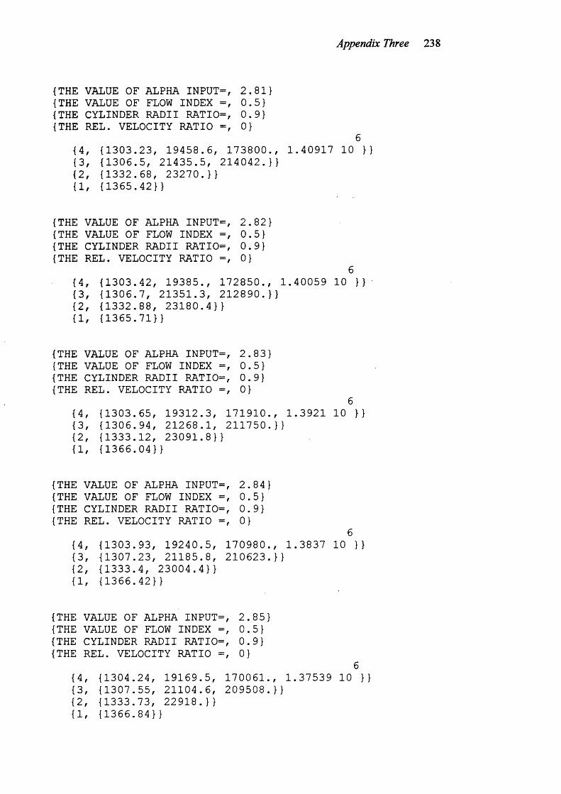
Appendix Three 238
{ THE VALUE O F A L P H A I N P U T = , 2 . 8 1 }{ THE VALUE O F FLOW I N D E X = , 0 . 5 }{ THE C Y L I N D E R R A D I I R A T I O = , 0 . 9 }{ THE R E L . V E L O C I T Y R A T I O = , 0}
6{ 4 , { 1 3 0 3 . 2 3 , 1 9 4 5 8 . 6 , 1 7 3 8 0 0 . , 1 . 4 0 9 1 7 1 0 }} { 3 , { 1 3 0 6 . 5 , 2 1 4 3 5 . 5 , 2 1 4 0 4 2 . } }{ 2 , { 1 3 3 2 . 6 8 , 2 3 2 7 0 . } }{ 1 , { 1 3 6 5 . 4 2 } }
{ THE VALUE O F A L P H A I N P U T = , 2 . 8 2 }{ THE VALUE O F FLOW I N D E X = , 0 . 5 }{ THE C Y L I N D E R R A D I I R A T I O = , 0 . 9 }{ THE R E L . V E L O C I T Y R A T I O = , 0}
6{ 4 , { 1 3 0 3 . 4 2 , 1 9 3 8 5 . , 1 7 2 8 5 0 . , 1 . 4 0 0 5 9 1 0 }} { 3 , { 1 3 0 6 . 7 , 2 1 3 5 1 . 3 , 2 1 2 8 9 0 . } }{ 2 , { 1 3 3 2 . 8 8 , 2 3 1 8 0 . 4 } }{ 1 , { 1 3 6 5 . 7 1 } }
{ THE VALUE O F A L P H A I N P U T = , 2 . 8 3 }{THE VALUE O F FLOW I N D E X = , 0 . 5 }{ THE C Y L I N D E R R A D I I R A T I O = , 0 . 9 }{THE R E L . V E L O C I T Y R A T I O = , 0}
6{ 4 , { 1 3 0 3 . 6 5 , 1 9 3 1 2 . 3 , 1 7 1 9 1 0 . , 1 . 3 9 2 1 1 0 }} { 3 , { 1 3 0 6 . 9 4 , 2 1 2 6 8 . 1 , 2 1 1 7 5 0 . } }{ 2 , { 1 3 3 3 . 1 2 , 2 3 0 9 1 . 8 } }{ 1 , { 1 3 6 6 . 0 4 } }
{ THE VALUE O F A L P H A I N P U T = , 2 . 8 4 }{THE VALUE O F FLOW I N D E X = , 0 . 5 }{ THE C Y L I N D E R R A D I I R A T I O = , 0 . 9 }{THE R E L . V E L O C I T Y R A T I O = , 0}
6{ 4 , { 1 3 0 3 . 9 3 , 1 9 2 4 0 . 5 , 1 7 0 9 8 0 . , 1 . 3 8 3 7 1 0 }} { 3 , { 1 3 0 7 . 2 3 , 2 1 1 8 5 . 8 , 2 1 0 6 2 3 . } }{ 2 , { 1 3 3 3 . 4 , 2 3 0 0 4 . 4 } }{ 1 , { 1 3 6 6 . 4 2 } }
{ THE VALUE O F AL P H A I N P U T = , 2 . 8 5 }{THE VALUE O F FLOW I N D E X = , 0 . 5 }{ THE C Y L I N D E R R A D I I R A T I O = , 0 . 9 }{ THE R E L . V E L O C I T Y R A T I O = , 0}
6{ 4 , { 1 3 0 4 . 2 4 , 1 9 1 6 9 . 5 , 1 7 0 0 6 1 . , 1 . 3 7 5 3 9 1 0 }} { 3 , { 1 3 0 7 . 5 5 , 2 1 1 0 4 . 6 , 2 0 9 5 0 8 . } }{ 2 , { 1 3 3 3 . 7 3 , 2 2 9 1 8 . } }{ 1 , { 1 3 6 6 . 8 4 } }
Appendix Four 239
APPENDIX FOUR COMPUTER PROGRAM FOR CONDUCTIVITY
MEASUREMENT AND CONTROL SYSTEM
C o n d u c t i v i t y p r o b e d a t a - l o g g i n g p r o g r a m
S e t - u p s y s t e m p a r a m e t e r s
10 3 0 5 0 7 0 9 0 110 1 3 01 5 0 V O L T S ( 0 ) = 0 1 7 0 B I N ( 0 ) = 01 9 0 B I T S l ( 0 ) = 0 : B I T S 2 ( 0 ) = 0 : B I T S 3 ( 0 ) = 0 2 1 0 C R L F $ = C H R $ ( 1 3 ) + C H R $ ( 1 0 )2 3 0 S A M P L E S = 3 5 0 2 5 0 C ONVR AT E %= 1 0 2 7 0 KEY 1 , " ! "2 9 0 KEY 2 , " œ "3 1 0 KEY 3 , " $ "3 3 0 KEY 4 , " % "3 5 0 KEY 1 0 , " ) "3 7 0 KEY 5 ,3 9 0 ON ERROR GOTO 5 0 7 0 4 1 0 CALL K D I N I T 4 3 0 '4 5 0 ' S e t - u p g r a p h p a r a m e t e r s 4 7 0 '4 9 0 F U L L S C A L E = 2 0 0 0 !5 1 0 WI ND0 WS%=15 3 0 DI M D A T A S L 0 T % ( 1 6 )5 5 0 D A T A S L O T % ( 0 ) = 1 : D A T A S L O T % ( 1 ) = 2 :
D A T A S L O T % ( 2 ) = 3 : D A T A S L O T % ( 3 ) = - l 5 7 0 DI M MI N Y ! ( 1 6 ) : DI M MAXYI ( 1 6 ) : N P T S ! = - 1 !5 9 0 Y M I N % = 0 : YMAX%=FULLSCALE6 1 0 FOR I N D X = 0 TO 1 6 : M I N Y I ( I N D X ) = Y M I N % : N E X T I NDX 6 3 0 FOR I N D X = 0 TO 1 6 : M A X Y I ( I N D X ) = Y M A X % : N E X T I NDX 6 5 0 '6 7 0 ' A l t e r c h a n n e l 0 t o l O O O m v F u l l s c a l e 6 9 0 MAXY!(0)=1000 7 1 0 '7 3 0 DI M C 0 L 0 U R % ( 1 6 )7 5 0 '7 7 0 ' M a i n p r o g r a m 7 9 0 '8 1 0 '
Appendix Four 240
8 3 08 5 08 7 08 9 09 1 09 3 09 5 09 7 0
9 9 01010
1 0 3 01 0 5 0
1 0 7 01 0 9 011101 1 3 01 1 5 01 1 7 01 1 9 012101 2 3 01 2 5 01 2 7 01 2 9 01 3 1 01 3 3 01 3 5 01 3 7 0
1 3 9 01 4 1 01 4 3 01 4 5 01 4 7 01 4 9 0
1 5 1 01 5 3 01 5 5 01 5 7 01 5 9 01 6 1 01 6 3 01 6 5 01 6 7 01 6 9 01 7 1 0
1 7 3 01 7 5 01 7 7 0
GOSUB 1 2 5 0L O C A T E 5 , 4 7 : P R I N T T I M E $I
' s a m p l e d o t p r o b e s 1 - 3I
C ALL F G R E A D ' ( " A N I N O " , " N O N E " , V O L T S ( ) , " C . M I L V L T " , " N T " )L OC AT E 1 8 , 1 2 : P R I N T U S I N G" # # # . # # " ; ( V O L T S ( 0 ) / l O O ) ; : P R I N T S P C ( 3 ) ;C AL L F G R E A D ' ( " A N I N l " , " N O N E " , V O L T S ( ) , " C . M I L V L T " , " N T " )L OC AT E 1 8 , 3 5 : P R I N T U S I N G" # # . # # # " ; ( V O L T S ( 0 ) / l O O O ) ; : P R I N T S P C ( 3 ) ;C AL L F G R E A D ' ( " A N I N 2 " , " N O N E " , V O L T S ( ) , " C . M I L V L T " , " N T " ) LOC AT E 1 8 , 5 8 : P R I N T U S I N G " # # # # " ; V O L T S ( 0 ) ; :P R I N T S P C ( 3 ) ;I
O P T K $ = I N K E Y $I F O P T K $ = " ) " THEN C L S : S Y S T E M : E N D I F O P T K $ = " o e " THEN GOSUB 1 7 7 0 I F O P T K $ = " % " THEN GOSUB 2 0 7 0 I F O P T K $ = " $ " THEN GOSUB 2 3 5 0 I F O P T K $ = " ! " THEN GOSUB 2 6 3 0 I F O P T K $ = " _ " THEN GOSUB 4 3 1 0 GOTO 8 7 0I
' M a i n m e n u s c r e e n
" T I M E $ ;
N u m b e r o f S a m p l e s " ;
CL SCOLOR 0 , 7P R I N T " C o n d u c t i v i t y D a t a A q u i s i t i o n P r o g r a m ( C) MRV 9 4
COLOR 7 , 0P R I N T : P R I N T : P R I N T : P R I N T P R I N T " D a t e " ; D A T E $ ; " T i m e P R I N T : P R I N T : P R I N T : P R I N T P R I N T " C o n v e r s i o n R a t eL OC AT E 9 , 5 8 : P R I N T S A M P L E S ; : LOCATE 9 , 2 2 : P R I N T CONVRATE%;L OC AT E 1 5 , 1 P R I N T "P R I N T "P R I N T "P R I N T "P R I N T "P R I N T "P R I N T "P R I N T : P R I N T COLOR 0 , 7 P R I N T " f l R u n F 5 R e v i e w f 1 0COLOR 7 , 0 RETURN
V I . 0 6 c
E I I I I I I I I I »°AAAAAAAAA°o oo o°AAAAAAAAA° ° P r o b e 1 ° E I I I I I I I I I ^
E I I I I I I I I I »° â a a a a M a a °o oo o° a M a a a a a a ° ° P r o b e 2 °
E I I I I I I I I I » " ° AAAAAAAAAA° "o o IIo ou° AAAAAAAAAA° " ° S p e e d R P M ° " È I I I I Ï I I I I I ^ "
f 2 F i l e s E x i t " ;
f 3 R a t e f 4 S a m p l e s
Appendix Four 241
1 7 9 0 ' F i l e s o p t i o n 1 8 1 0 '1 8 3 0 '1 8 5 0 C L S1 8 7 0 P R I N T : P R I N T : P R I N T " C u r r e n t D a t a F i l e s "1 8 9 0 P R I N T " ____________________________________________________1 9 1 0 P R I N T1 9 3 0 S H E L L " c d \ k d a c \ d a t a 1 9 5 0 F I L E S1 9 7 0 H O L D $ = I N K E Y $ : I F H O L D $ = " " THEN 1 9 7 0 1 9 9 0 O P T K $ = " 9 9 "2 0 1 0 S H E L L " C D \ K D A C \ R U N 2 0 3 0 GOSUB 1 2 5 0 2 0 5 0 RETURN 2 0 7 0 '2 0 9 0 ' S e t s a m p l e s o p t i o n 2110 '
2 1 3 0 '2 1 5 0 L OCATE 9 , 5 8 : P R I N T S P C ( 6 )2 1 7 0 COLOR 0 , 72 1 9 0 L OCATE 9 , 5 8 : P R I N T S P C ( 4 )2 2 1 0 LOCAT E 9 , 5 8 : I N P U T " " , C S A M P L E S $2 2 3 0 COLOR 7 , 0 2 2 5 0 C S A M P L E S = V A L ( C S A M P L E S $ )2 2 7 0 I F ( C S A MP L E S > 9 9 9 9 ) OR ( C S A M P L E S = 0 ) THEN
S A M P L E S = S A M P L E S E L S E S A M P L E S = C S A M P L E S 2 2 9 0 L OCATE 9 , 5 8 : P R I N T S P C ( 1 5 )2 3 1 0 L OCATE 9 , 5 8 : P R I N T S AMP LES 2 3 3 0 RETURN 2 3 5 0 '2 3 7 0 ' S e t s a m p l e r a t e o p t i o n 2 3 9 0 '2 4 1 0 '2 4 3 0 LOCATE 9 , 2 2 : P R I N T S P C ( 6 )2 4 5 0 COLOR 0 , 72 4 7 0 LOCATE 9 , 2 2 : P R I N T S P C ( 4 )2 4 9 0 LOCATE 9 , 2 2 : I N P U T " " , CCONVRATE$2 5 1 0 COLOR 7 , 02 5 3 0 C C O N V R A T E = V A L ( C C O N V R A T E $ )2 5 5 0 I F ( CCONVRATE > 9 9 9 9 ) OR ( C C O N V R A T E = 0 ) THEN
CONVRATE%=CONVRATE% E L S E CONVRATE%=CCONVRATE 2 5 7 0 LOCATE 9 , 2 2 : P R I N T S P C ( 1 5 )2 5 9 0 LOCATE 9 , 2 2 . «PRI NT CONVRATE%2 6 1 0 RETURN2 6 3 0 ' R u n t i m e r o u t i n e 2 6 5 0 2 6 7 0 2 6 9 0 2 7 1 02 7 3 0 CALL BG R E A D '
( " A N D A T A " , s a m p l e s , " A N I N O , A N I N l , A N I N 2 " , 1 , " N O N E " , 1 , " N T " , " T A S K l " )
S e t u p b a c k g r o u n d r e a d f o r n s a m p l e s & n o t r i g
Appendix Four 242
2 7 5 0 '2 7 7 0 ' S e t u p i n t e r u p t i n t e r v a l f o r n m i l i s e c s
t o g i v e r e q u i r e d s a m p l e 2 7 9 0 ' p e r i o d 2 8 1 0 '2 8 3 0 RATE%=CONVRATE%2 8 5 0 C AL L I N T O N ' ( r a t e % , " M I L " )2 8 7 0 '2 8 9 0 ' G r a p h d a t a 2 9 1 0 '2 9 3 0 S C R E E N 22 9 5 0 C ALL G R L A B E L ' ( " C o n d u c t i v i t y / R P M " , 1 , 1 , " L E F T " , " C T R " ) 2 9 7 0 C A L L G R L A B E L ' ( " R e a l t i m e p l o t o f c o n d u c t i v i t y
p r o b e s " , 1 , 1 , " T O P " , " C T R " )2 9 9 0 C AL L H G R A P H R T ' ( " A N D A T A " , D A T A S L O T % ( ) , " F A S T " ,
M I N Y ! 0 , M A X Y ! ( ) , " C . M I L V L T " , N P T S ! , W I N D O W S % , " G R I D " ) 3 0 1 0 '3 0 3 0 ' T u r n o f f i n t e r u p t s , s a v e & d e l e t e a r r a y 3 0 5 0 '3 0 7 0 C AL L I N T O F F3 0 9 0 S C R E E N 03 1 1 0 GOSUB 3 2 3 03 1 3 0 C AL L A R D E L ' ( " a n d a t a " )3 1 5 0 '3 1 7 0 C ALL K D I N I T 3 1 9 0 GOSUB 1 2 5 0 3 2 1 0 RETURN 3 2 3 0 '3 2 5 0 ' F i l e s a v e3 2 7 0 ' '3 2 9 0 '3 3 1 0 C L S 3 3 3 0 P R I N T3 3 5 0 P R I N T " F i l e S a v e P r e s s e n t e r t o q u i t "3 3 7 0 P R I N T " "3 3 9 0 P R I N T3 4 1 0 I N P U T " E n t e r F i l e n a m e " ; F I L E $3 4 3 0 F I L E $ = L E F T $ ( F I L E $ , 8)3 4 5 0 I F F I L E $ = " " THEN 4 2 1 0 3 4 7 0 S F I L E $ = F I L E $ + " . S 5 0 "3 4 9 0 A F I L E $ = F I L E $ + " . T X T "3 5 1 0 '3 5 3 0 ' U s e r e n t e r e d v a r i a b l e s 3 5 5 0 DATA C o m m e n t , C o n d u c t i v i t y R a n g e # 1 ,
C o n d u c t i v i t y R a n g e # 2 3 5 7 0 '3 5 9 0 ' C r e a t e h e a d e r o n d a t a f i l e i n CS V f o r m a t 3 5 9 5 P R I N T3 6 1 0 P R I N T " S a v i n g a s c i i d a t a t o " ; T A B ( 3 0 ) A F I L E $3 6 3 0 S H E L L " C D \ K D A C \ A S C I I3 6 5 0 OP EN A F I L E $ FOR OUTP UT AS # 13 6 7 0 P R I N T # 1 , C F I L E $ : P R I N T3 6 9 0 FOR LOOP = 1 TO 33 7 1 0 READ I N F O $ : P R I N T I N F O $ ; : P R I N T T A B ( 3 0 ) ;
Appendix Four 243
3 7 3 0 I N P U T " > " , P A R A M $3 7 5 0 P R I N T # 1 , P A R A M $3 7 7 0 NEXT L OOP 3 7 9 0 '3 8 1 0 ' A d d d a t e & T i m e3 8 3 0 P R I N T # ! , " D a t e " ; D A T E $ ; " , " ; " T i m e " T I M E $3 8 5 0 '3 8 7 0 ' C r e a t e a s c i i d a t a f i l e i n CSV f o r m a t3 8 7 5 P R I N T3 8 7 6 P R I N T " S a v i n g D a t a > " ;3 8 9 0 M I L V l ( 0 ) = 0 : M I L V 2 ( 0 ) = 0 : M I L V 3 ( 0 ) = 0 : D O N E % = 03 9 1 0 P R I N T # ! , " C o n d u c t i v i t y # 1 , C o n d u c t i v i t y # 2 , M o t o r , T i m e "3 9 3 0 P R I N T # ! , " u S , u S , R P M , m s "3 9 5 0 FOR L 0 0 P = 1 TO S AMP LES3 9 7 0 CALL A R G E T ' ( " A N D A T A " , L O O P , L O O P , " A N I N O " ,
1 , M I L V l 0 , " C . M I L V L T " )3 9 9 0 C ALL A R G E T ' ( " A N D A T A " , L O O P , L O O P , " A N I N l " ,
1 , M I L V 2 0 , " C . M I L V L T " )4 0 1 0 C ALL A R G E T ' ( " A N D A T A " , L O O P , L O O P , " A N I N 2 " ,
1 , M I L V 3 0 , " C . M I L V L T " )4 0 3 0 P R I N T # 1 , M I L V 1 ( 0 ) / 1 0 0 ; " , " ; M I L V 2 ( 0 ) / 1 0 0 0 ; " , " ;
M I L V 3 ( 0 ) ( L O O P - 1 ) * R A T E %4 0 3 5 D0NE%=D0NE% + 1 : I F DONE %= 1 0 THEN P R I N T " . " ; : DONE%=04 0 5 0 NEXT LOOP4 0 5 5 R E S T O R E4 0 7 0 C L O S E # 14 0 9 0 '4 1 1 0 ' C r e a t e r a w d a t a f i l e 4 1 3 0 S H E L L " C D \ K D A C \ D A T A 4 1 3 5 P R I N T : P R I N T4 1 5 0 P R I N T " S a v i n g r a w d a t a t o " ; T A B ( 3 0 ) S F I L E $4 1 7 0 C ALL A R S A V E ' ( " A N D A T A " , S F I L E $ , " C . M I L V L T " ,
" F T . K D A C " , RAT E %, " H M I C " )4 1 9 0 '4 2 1 0 S H E L L " C D \ K D A C \ R U N "4 2 3 0 RETURN 4 2 5 0 '4 2 7 0 ' R e v i e w d a t a4 2 9 0 ' '4 3 1 0 '4 3 3 0 C L S4 3 5 0 P R I N T : P R I N T4 3 7 0 P R I N T " F i l e R e v i e w P r e s s e n t e r t o q u i t "4 3 9 0 P R I N T " "4 4 1 0 P R I N T4 4 3 0 I N P U T " E n t e r F i l e n a m e " ; F I L E $ 4 4 5 0 F I L E $ = L E F T $ ( F I L E $ , 8 )4 4 7 0 I F F I L E $ = " " THEN 4 9 1 0 4 4 9 0 F I L E $ = F I L E $ + " . S 5 0 "4 5 1 0 A R R A Y $ = S P A C E $ ( 2 5 5 )4 5 3 0 S H E L L " C D \ K D A C \ D A T A 4 5 5 0 D A T A D E P T H ! = 0 ! : DAT AWI DT H%=0
: L A S T P O I N T ! = 0 ! : L A B L $ = S P A C E $ ( 2 5 5 ) 4 5 7 0 '

Appendix Four 244
4 5 9 0 C O L O U R % ( 0 ) = 3 : C O L O U R ! ( 1 ) = - 1 4 6 1 0 '4 6 3 0 ' R e a d a r r a y f r o m d i s k 4 6 5 0 '4 6 7 0 CALL A R L O A D ' ( A R R A Y $ , F I L E $ )4 6 9 0 '4 7 1 0 ' G r a p h d a t a 4 7 3 0 '4 7 5 0 CALL A R S T A T U S ' (A R R A Y $ , D A T A D E P T H ! ,
D A T A W I D T H ! , L A S T P O I N T ! , L A B L $ )4 7 7 0 P R I N T : P R I N T : P R I N T " -------- D a t a f i l e l o a d e d ------ " : P R I N T4 7 9 0 P R I N T : P R I N T : P R I N T " P r e s s a n y k e y w h e n r e a d y "4 8 1 0 H O L D $ = I N K E Y $ : I F H O L D $ = " " THEN 4 8 1 0 4 8 3 0 S C R E E N 2 4 8 5 0 C ALL G R A P H '
( A R R A Y $ , D A T A S L O T ! ( ) , C O L O U R ! ( ) , " S C R O L L " , 0 . , F U L L S C A L E , " N O R M A L " , 1 , 1 . , D A T A D E P T H ! , " C . M I L V L T " )
4 8 7 0 CALL A R D E L ' ( A R R A Y $ )4 8 9 0 '4 9 1 0 S C R E E N 0 4 9 3 0 S H E L L " C D \ K D A C \ R U N 4 9 5 0 GOSUB 1 2 5 0 4 9 7 0 RETURN 4 9 9 0 '5 0 1 0 ' E R R O R T r a p 5 0 3 0 5 0 5 0
I
5 0 7 0 P R I N T : P R I N T " s y s t e m e r r o r @ l i n e " ; E R L ;" i n v a l i d f i l e n a m e s y s t e m w i l l r e t r y "
5 0 9 0 FOR P A U S E = 0 TO 9 0 0 0 : NEXT P AUS E 5 1 1 0 I F E R L = 4 6 7 0 THEN RESUME 4 3 1 0 5 1 3 0 I F E R L = 3 6 5 0 THEN RESUME 3 2 9 0 5 1 5 0 P R I N T : P R I N T " u n a b l e t o i d e n t i f y e r r o r
s y t e m w i l l r e - s t a r t "5 1 7 0 FOR P A U S E = 0 TO 9 0 0 0 : NEXT P AUS E 5 1 9 0 S C R E E N 0 : R U N 5 2 0 0 END
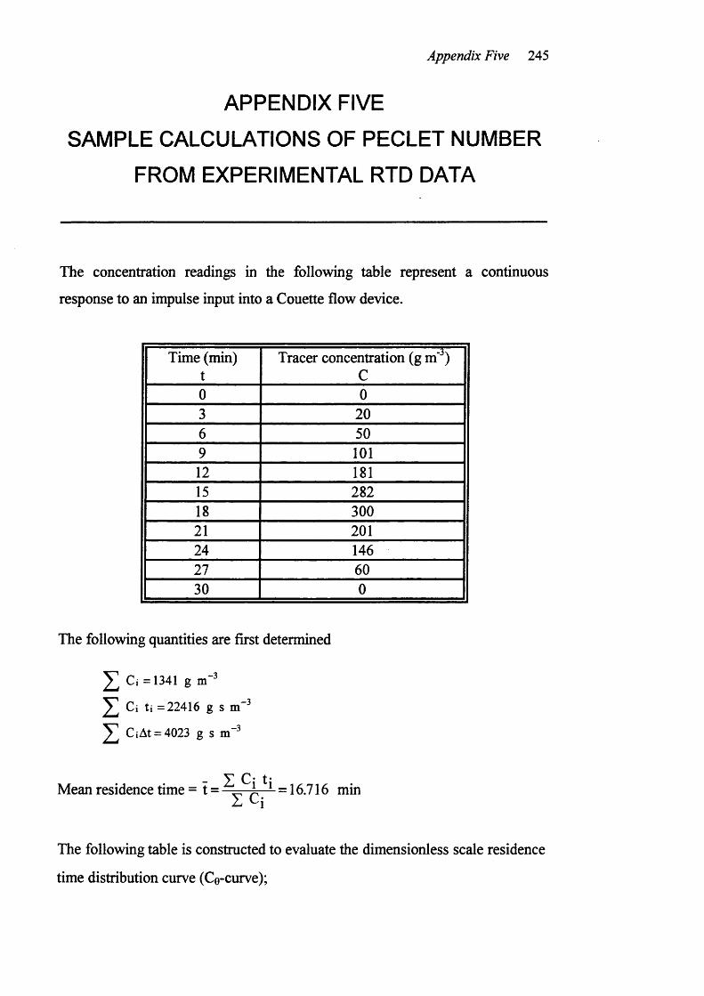
Appendix Five 245
APPENDIX FIVE
SAMPLE CALCULATIONS OF PECLET NUMBER
FROM EXPERIMENTAL RTD DATA
The concentration readings in the following table represent a continuous
response to an impulse input into a Couette flow device.
Time (min) t
Tracer concentration (g m' ) C
0 03 206 509 10112 18115 28218 30021 20124 14627 6030 0
The following quantities are first determined
^ Ci =1341 g m"
^ Ci ti =22416 g s :
CiAt = 4023 g s m
- 3
y c* t-Mean residence time = t= ^ ^ =16.716 min
Z Ci
The following table is constructed to evaluate the dimensionless scale residence
time distribution curve (Ce-curve);
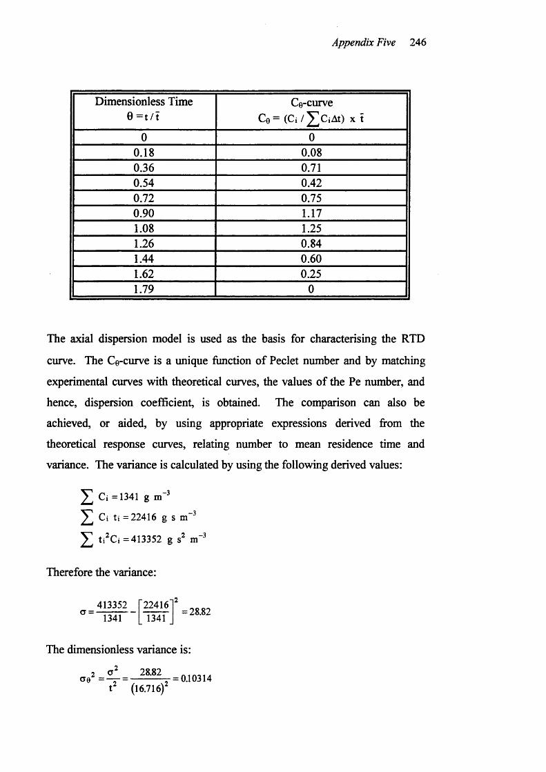
Appendix Five 246
Dimensionless Time 0 = t / t
Ce-curve Ce= ( C i / ^ C i A t ) X t
0 00.18 0.080.36 0.710.54 0.420.72 0.750.90 1.171.08 1.251.26 0.841.44 0.601.62 0.251.79 0
The axial dispersion model is used as the basis for characterising the RTD
curve. The Ce-curve is a unique function of Peclet number and by matching
experimental curves with theoretical curves, the values of the Pe number, and
hence, dispersion coefficient, is obtained. The comparison can also be
achieved, or aided, by using appropriate expressions derived from the
theoretical response curves, relating number to mean residence time and
variance. The variance is calculated by using the following derived values:
^ Ci = 1341 g
y Ci ti = 22416 g s
^ ti^Ci = 413352 g
Therefore the variance:
CT = 4133521341
224161341
= 28.82
The dimensionless variance is:
28.82
(16.716)'= 0.10314
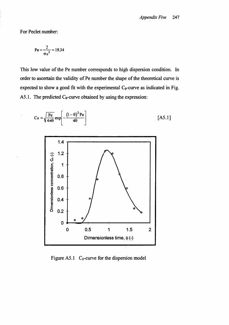
Appendix Five 247
For Peclet number:
Pe =ae
= 1934
This low value of the Pe number corresponds to high dispersion condition. In
order to ascertain the validity o f Pe number the shape of the theoretical curve is
expected to show a good fit with the experimental Ce-curve as indicated in Fig.
A5.1. The predicted Ce-curve obtained by using the expression:
Ce _U n e exp
( 1 - e f P e4 6
[A5.1]
1.4
1.2 - -
0.8
0.6 -
0.4 -
0.2 -
0.5 1 1.5Dimensionless time, e (-)
Figure A5.1 Ce-curve for the dispersion model
Appendix Six 248
APPENDIX SIX
PUBLISHED PAPER RELATING TO
THIS PROJECT
Summary of Research Outputs
Papers Published
Samson S. S. Yim and P. Ayazi Shamlou, 1996. Residence TimeDistribution In A Rotary Flow-Throush Device. Fluid Mixing 5: IChemE Symp. Ser. 140, 191-201.
Samson S. S. Yim and P. Ayazi Shamlou, 1996. The Effect of Geometry On Mixing Performance In Continuous Couette-flow Devices. Proceedings: 5th World Congress Of Chemical Engineering, 1, 647-652.
Samson S. S. Yim and P. Ayazi Shamlou, 1996. Residence TimeDistribution In A Rotary Flow-through Device. Proceedings: IChemE Research Events/Second European Conference for Young Researchers, 2, 955-957.
Samson S. S. Yim and P. Ayazi Shamlou, 1996. Residence TimeDistribution (RTD) In A Rotary Flow-through Device with non-Newtonian Fluids. AIChE Annual Meeting (Oral presentation and hill paper).
Papers Accepted
Samson S. S. Yim , N. Titchener-Hooker and P. Ayazi Shamlou, 1997. Prediction o f Critical Taylor Number For Non-Newtonian Fluids. The First European Congress on Chemical Engineering. (Oral presentation and full paper).
Samson S. S. Yim and P. Ayazi Shamlou, 1997. Prediction of Critical Tavlor Number in Rotating Flow-through Devices. Proceedings: 1997 Jubilee Research Events.
Appendix Six 249
Papers Submitted
Samson S. S. Yim and P. Ayazi Shamlou, 1996, Factors affecting flow instability of Newtonian liquids in Couette-Poiseuille flow. Full paper submitted for publication to Chemical Engineering Science.
Research Awards
University College London-Graduate School Exhibition -1993 M A P S , E n g i n e e r i n g a n d T h e B u i l t E n v i r o n m e n t P r i z e A w a r d
University College London-Graduate School Exhibition - 1995 M A P S , E n g i n e e r i n g a n d T h e B u i l t E n v i r o n m e n t P r i z e A w a r d
Appendix Six 250
Papers PublishedSamson S. S. Yim and P. Ayazi Shamlou, 1996. Residence Time Distribution In A Rotary Flow-Through Device. Fluid Mixing 5: IChemE Symp. Ser. 140, 191-201.
ICHEME SYMPOSIUM SERIES NO. 140
R e s id e n c e T im e D is t r ib u t io n In A R o t a r y F l o w -T h r o u g h D e v ic e
Samson S. S. Yim and Ayazi Shamlou P.Chemical and Biochemical Engineering, University College London. London WCIE 7JE
Residence time distribution (RTD) experiments were earned out to investigate the critical conditions for the establishment of near plug flow of a Newtonian liquid flowing through the gap of a horizontal coaxial cylinder device. The operating conditions in the annulus could be varied between the laminar flow and Taylor-Couette-Poiseuille flow. The RTD curves were described using a single parameter axial dispersion model. The results suggested significant variations from plug flow conditions depending on the axial Reynolds number and Taylor number.
Keywords: Residence Time Distribution, Coaxial Cylinder,Taylor-Couette-Poiseuille flow, Taylor number.Axial dispersion model.
IN T R O D U C T IO N
Many operations in the chemical, biochemical and food process industries involve the continuous transport of materials through rotating equipmenL Examples include émulsification, polymerization, solvent extraction, crystallization, precipitation, mixing and heat transfer operations (1,23,4,5). A coaxial cylinder device consisting o f a stationary outer shell and a rotating iiuier cylinder with or without blades and wipers is Aequently used in these operations because of its ability to promote good radial mixing and negligible axial dispersion (6,7). These flow characteristics are prerequisite when trying to optimize any operations occurring in the rotating flow through device. In solvent extraction applications, for example, deviations from plug flow can result in a significant reduction in the mass transfer driving forces and thus the separation efficiency of the equipment can be determintally affected (8).
The rational design of a rotating coaxial cylinder device with superimposed axial flow requires knowledge of the fluid flow panems and mixing in the equipment The complex flow panems produced in the gap between the two cylinders strongly depend on the rotational speed, axial flow rate, gap width and the theological properties o f the material (9,10,11,12). In the absence of any superimposed axial flow, for relatively low rotational speeds of the inner cylinder the liquid flow in the aimular gap is laminar (Couette) flow and the prevailing
191
Appendix Six 251
ICHEME SYMPOSIUM SERIES NO. 140
radial velocity profile of the liquid causes significant dispersion. As the rotational speed increases the flow structure becomes unstable characterized by the appearance of a series of (Taylor) vortex cells formed at regular intervals along the axis of the cylinder (12). The condition at which the vortices first appear is usually expressed in terms of a critical Taylor number, Ta . In the prevailing laminar vortex (Taylor-Couene) flow regime, there is negligible interaction between the neighboring cells but within each cell the toroidal motion of the fluid causes good radial mixing (1,7). When a small axial flow is added to the Taylor- Couette flow, the cells maintain their separate identity but move along the gap at a constant velocity determined by the flow rate. This type of flow is generally referred to as Taylor- Couette-Poiseuille flow and provides hydrodynamic conditions in the equipment which closely approach those of plug flow(7,l 1). With further increase in the rotational speed of the inner cylinder or the axial flow rate the vortices develop circumferential waves causing exchange of material at their boundaries (1). As a result axial dispersion increases and flow deviates from the ideal plug flow conditions. The flow regime in the armulus gradually changes from wavy vortex flow to turbulent vortex flow and fully turbulent flow as rotational speed of the inner cylinder increases (11).
The transitions between the various flow regimes are strong functions of the dimensionless
axial Reynolds number. Re dimensionless rotational Taylor number. Ta
= , and the dimensionless gap width, n [= • Of particular interest
to this study is the effects of Re and Ta numbers on the extent of mixing in the Taylor- Couette-Poiseuille (TCP) flow. Surprisingly few publications have addressed this aspect (1,2). The aim of the present study is to provide axial dispersion data obtained from residence time distribution (RTD) experiments carried out in a horizontal coaxial cylinder device operating in the TCP flow regime.
EXPERIMENTAL
The residence time distribution experiments were performed by using an impulse tracer injection technique. The experiments were directed towards determining the influence of the rotational speed of the inner cylinder and axial flow rate on the RTD of a 60 % glycerol-water solution. The rotational speed was varied between 30 and 350 rpm and the volumetric flow rate was changed between 1x10 and 4x10^ nun Vs.
All the experiments reported in this study were carried out in a 1 m long horizontal coaxial cylinder device which is shown in Fig. 1. The iiuier rotating cylinder was constructed from a
192
Appendix Six 252
ICHEM E S Y M PO SIUM S E R I E S NO. 140
stainless steel tube having an outside diameter of 76 mm and driven by a variable speed electric motor with rotational speed in the range of 0 • 1000 rpm. The speed of rotation was measured by using a shaft-mounted speed transducer (EEL Ltd., Westland Aerospace, East Cowes, Isle of Wight, UK). The outer shell was fabricated from Perspex to allow visual observations of the flow structure and had an inner diameter of 90 mm. The annular gap formed by the two cylinders was 7 mm wide giving a ratio of the outer to inner tube diameter o f 1.18.
The outer shell was equipped with two electrical conductivity probes and a single injection point. The conductivity probes were constructed from 35 rtun diameter glass rod, having two0.315 mm diameter platinum wire electrodes mounted 2.5 mm apart. The two probes were separated 600 mm apart in a horizontal line with the first probe positioned 50 mm from the injection point. When in position, the tip of the electrodes protruded 3 mm from the inside wall of the outer shell. The microinjector was a standard hypodermic syringe having a stainless tube of 0.7 mm outside diameter. The injection point was 200 mm h’om the entrance in the same horizontal line as the conductivity probes and the tip of the injection tube was positioned at the centre of annular gap. The tracer solution was prepared from concentrated KCl (BDH Supplies) and the working liquid. Injection was carried out manually within a period of approximately 1.0 s and the tracer concentrations were determined simultaneously and continuously at the two probe positions as a function of time. The data from both conductivity probes were stored using a data acquisition system (Keithley Model 575 measurement control system attached to a KDAC 500/1 data collection unit and a IBM PC2 computer) for analysis and evaluation of the various parameters including the first and second moments of the distributions.
Prior to injection of the tracer materiaL steady state flow condition was established in the device by continually pumping (Watson-Marlow Ltd., UK) the working liquid through the aruiular gap at a fixed volumetric flow rate until the efflux remained constant with time. The efflux was obtained manually by measuring the time required to collect a known volume of the discharge liquid.
Each experiment was replicated three times and the mean value used for parameter estimation.
RESULTS AND DISCUSSION
The experimental RTD C-curves obtained from the second probe are shown in Fig. 2 for a range of rotational speed of the inner cylinder. Initially the same experiment was repeated three times to gain experience in conducting the measurements and also to check the
193
Appendix Six 253
ICHEME SYMPOSIUM SERIES NO. 140
reproducibility of the data. It was found that the time taken for the injection of the tracer material had a significant effect on the reproducibility of the results and the subsequent fit of data. By trial and error, the best injection time was found to be less than 2 seconds for which the RTD measurements were reproducible to ±5%. All data reported in the present study fall in this range. The data in Fig. 2 refer to a flow rate of 1.5x10^ mm^/s. The tracer concentrations are presented in dimensionless form defined as C(t)/Co, where C(t) is the tracer concentration measured by each probe at time t following the introduction of the tracer impulse. C, is the total concentration of the tracer material obtained from the area under the tracer response curve. Figure 3 shows the effect of superimposed axial flow rate on the RTD curves for a rotational speed of 100 rpm. The plots in Figs 2 and 3 indicate that either an increase in the rotational speed or a decrease in the axial flow rate results in a broadening of the RTD curves and a consequential deviation from plug flow conditions.
According to previous studies (2,13,14.15) the transition from Couette flow to Taylor vortex flow occurs in the range of Taylor numbers between 40 and 80 depending on the axial Reynolds number and the gap width. An examination of the data shown in Figs 2 and 3 indicate the existence of Taylor vortex flow under most of the experimental conditions.
Typical RTD curves for the two probes are shown in Fig. 4 for a rotational speed of 110 rpm and axial flow velocity of 20 mm/s corresponding to an axial Reynolds number. Re = 25 and Taylor number. Ta = 121. The two response curves in Fig. 4 show that a vortex cell takes approximately 25 s (peak to peak time) to travel between the two probes and noting that the distance between the probes was fixed at 600 mm gives a (vortex) shift velocity of about 24 mm/s which is reasonably close to the. average axial liquid velocity in the gap. This is in good agreement with previous results (1,7).
The RTD curve can be mathematically modeled by using its various moments. In many cases however, the first and second moments provide an adequate description of the distribution and will therefore be used in the present study. The first moment of the RTD curve gives the mean residence time and is defined as
(Tcdt
jpd.
The mean residence time, i , can also be obtained directly from the axial flow rate and the working volume of the equipment. Thus
194
Appendix Six 254
ICHEME SYMPOSIUM SERIES NO. 140
V (2)
The dimensionless time, 9, is defined as
T L(3)
where v is the axial liquid velocity and L the distance between the two probe positions.The second moment of the RTD curve gives the variance of the distribution and is defined as
a" (t) =fC d t
(4)
and the dimensionless variance, o(6), defined as
o " (0 )= c - ( t )(5)
The flow of the tracer material in the annular gap of a coaxial cylinder device has been described adequately by an axial dispersion model ( 17,18). For the experiments carried out in the present investigation an impulse was injected into the gap at an arbitrary time, t = 0. Prior to the injection, the tracer concentration in the gap was zero and following the input of the tracer, its concentration was measured at two positions in the gap. These are the boundary conditions that describe an open-open system ( 17) and the partial differential equation of the dispersion concerned with an impulse measurement technique in this type of system has been solved analytically ( 17). The dimensionless tracer concentration, C(6), at the measuring point for the prevailing conditions is given by
(i-ey40
Pe (6)
assuming no stagnant region and negligible short circuiting of the liquid in the gap. In Eq. 6, the dimensionless Peclet number. Pe = vL/D, and the dimensionless tracer concentration, C(0), at dimensionless time 0, C(0) = CftyCp.
195
Appendix Six 255
ICHEME SY M P O S IU M S E R I E S NO. 140
The axial dispersion coefficient. D, can be obtained from the definition of the Pe number.
(vL / D ), which in turn is related to the variance of the distributions by (17)
Ac^(0) = — (7)
Aa^(6) represents the variance difference of the tracer RTD curves at any two points along the annular gap. In the present study Aa^(0) was determined between the two probe positions using the experimental response curves obtained from them, as shown in Fig. 4. The value of Ao^(0) was substituted into Eq. 7 in order to obtain the Pe for the prevailing flow and hence the axial dispersion coefficient, D. Finally, the Pe number was used together with Eq. (6) to fits the observed time variation of the tracer concentration C(t) at the two probe positions. The agreement of the experimental tracer RTD curves for the liquid in the gap with Eq. 6 was satisfactory, as shown in Fig. 5 for all the conditions examined in this work.
The effect of the rotational speed on the Pe. obtained from the impulse response curves at the two conductivity probe positions is shown in Fig. 6 for two axial flow rates expressed as Reynolds number. The plots on Fig. 6 shows that as the rotational speed of the inner shaft increases, the Pe number increases from an initial value of about 30 to a maximum value of approximately 250 beyond which any further increase in rotational speed causes a decrease in the Pe number. The minimum and maximum values of the Pe number were found to be a function of the flow rate through the device. In the experiments carried out in the present study the lowest value of Pe was found to be about 30 corresponding to a axial flow rate of 7.2 mm/s (Re =11) and the highest value of Pe was 250 as shown in Fig. 6.
The variations in Pe number with increasing Ta number depicted in Fig. 6 suggest that significant deviations from plug flow conditions can occur in the vessel during flow. Coney and Simmers (18), Ogawa ei al.(]9) and Astill (20) carried out detailed studies of the flow instability in the Taylor vortex flow as function of both rotational speed and axial flow rate. These investigations revealed that the vortices first appear in the annulus next to the wall of the rotating shaft. As the speed of the inner shaft increases the vortices grow in size until they eventually reach the walls of the outer stationary cylinder (18,19,20). Pudjiono ei al.(2) in their recent publication argued that the maximum Pe number corresponded to the conditions at which the Taylor vortices were fully developed. These observations regarding the birth and growth of vortices suggest that the transition from Couette flow to fully developed Taylor vortex flow occurs over a period of time and range of speed. In other words there is not a single speed at which flow regime suddenly changes as that speed is reached. The data presented in Fig. 6 are insufficient to allow firm conclusions to be made about the causes for the observed dependency of Pe on Re and Ta, but the general trend in
196
Appendix Six 256
ICHEME SYM POSIUM S E R I E S NO. 1 4 0
data shown in Fig. 6 appear to support the work Pudjiono ei a/.(2) and the general observations o f others (18,19^0).
CONCLUSIONS
Residence time distribution data were obtained for the dispersion of a impulse injection of tracer in the gap of a coaxial cylinder device operating in the Taylor-Couette-Poiseuille regime. The RTD data were described by using an axial dispersion model and the results suggested that significant deviations from plug flow can occur depending on the prevailing Taylor number and axial Reynolds number.
NOMENCLATURE
C(t) = tracer concentration at time t (mol/litre)Co = total tracer concentration (mol/litre)C(9) = dimensionless tracer concentration (Eq. 6) (-)d = annular gap (Ro-R;) (m)D = axial dispersion coefficient (m^ s ')L = distance between two measuring points (m)
n = dimensionless gap width (-)
N = rotational speed of inner cylinder (rps)
fPe = Peclet number. I (-)
Q = volumetric flow rate of liquid (m^ s ')Ro = radius of the outer shell (m)Rj = radius of the inner cylinder (m)
Re = axial Reynolds number. (.)
Ta = Taylor number.p (2 n N )R o à I d (-)P \ Ro
Ta, = critical Taylor number (-)t = time (s)V = working volume of the equipment (m^)V = axial flow velocity through the gap (m s ')T = mean residence time (s)
197
Appendix Six 257
ICHEME SYM POSIUM S E R I E S NO. 14 0
6 = dimensionless time (Eqs 1 and 2) (-)a(t) = variance of the distribution at time t (-)<y(0) = dimensionless variance (Eq. 6) (-)p * density of the working liquid (kg m'^)H - viscosity of the working liquid (kg m ' s ')
REFERENCES
1. Kataoka, K. and Takigawa, T., 1981. AlChE J.. 27; 504-508.2. Pudjiono. P.I., Tavare, N.S.. Garside. J. and Nigam. K.D.P.. 1992. Chem. Engng J..
101 - 110 .
3. Abichandani, H. and Sarma, S.C.. 1988. Chem. Engns Sci.. 43: 871-881.4. Hoare. M., Narendranathan. TJ.. Flint, J.R.. Heywood-Waddington. D., Bell. DJ. and
Dunnill. P., 1982, l&EC Fundam.. 21: 402-406.5. Dongaonkar, K.R., Pratt, H.R.C. and Stevens. G.W., 1991. AlChE J.. 37: 694-704.6. Legrand. J. and Coeuret, F., 1986, Chem. Engng Sci.. 4 1 : 47-53.7. Kataoka, K., Doi, H.. Hongo, T. and Futagawa, M., 1975, J. Chem. Engng Japan. 8:
472-476.8. von Stockar, U. and Lu, X.. 1991. Ind. Engng. Chem. Res.. 30: 1248-1257.9. Coles, D., 1965, J. Fluid Mech.. 21: 385-425.10. Croockewit, P., Honig, C.C. and Kramers. H.. 1955. Chem. Engng Sci.. 4: 111-118.11. Harrod. M.. 1986, J. Food Proc. Engng.. 9: 1 -62.12. Taylor. G.I., 1923. Phil. Trans.. A233: 289-343.13. Ng. S. and Turner. E. R., 1982, Proc. Rov. Soc. Lond.. A 382: 83-102.14. Takeuci, D. I. and Jankowski, D. F., 1981. J. Fluid Mech.. 102: 101-126.15. Hasoon, M. A., and Martin, B. W., 1977, Proc. Rov. Soc. Lond.. A 352: 351-380.16. Danckwerts. P.V.. 1953. Chem. Engng Sci.. 2: 1-13.17. Levenspiel. O., 1979, Chemical Reaction Engineering, Wiley, New York. Chapter IX.18. Coney, J.E.R. and Simmers. D.A., 1979. J. Mech. Engng Sci.. 21: 19-24.19. Ogawa, A., Fujita, V. and Nagabayashi, N.. 1985, Chem. Engng Commun.. 37; 209-
222.
20. Astill. K.N., 1964, J. Heat Transfer. 8: 383-392.
198
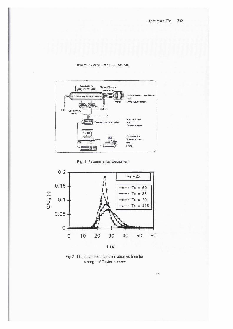
Appendix Six 258
ICHEME SYMPOSIUM SERIES NO. 140
I ConducbvKy Sp.eb/ro™» transducer
ConductMty meter
Rotary Sowinrouch device
Outlet
_ Rotary Hovnnrough device Æji and
motor ConducDvty meters
Measurement Data acquisition system and
Control system
Computer torScreen monitor
Pnnter
Fig. 1 Experimental Equipment
0.2Re = 25
0.15
ü° 0.1 Ü
0.05
: Ta = 201
0 10 20 30 40 50 60
t (s)
Fig.2 Dimensionless concentration vs time for a range of Taylor number
1 9 9
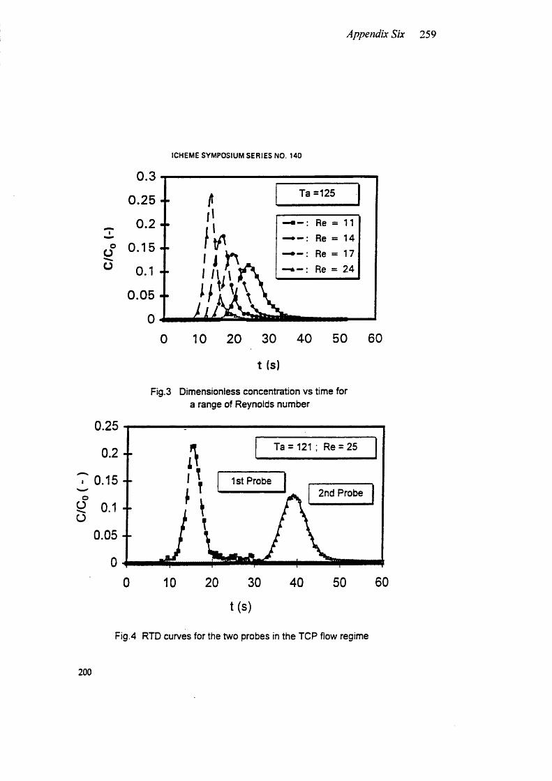
Appendix Six 259
OO
IC HEM E SY M PO SIUM S E R I E S NO. 1 4 0
0.3Ta =1250.25
0.2Re = 14 Re = 170.15
.1
0.05
0
10 20 30 40
t (s)
50 60
Fig.3 Dimensionless concentration vs time for a range of Reynolds number
0.25Ta = 121 : Re = 250.2 . .
0.15 -- 1st ProbeI2nd Probe
0.05 --
0 10 20 30 40 50 60
t(s)
Fig.4 RTD curves for the two probes in the TCP flow regime
200
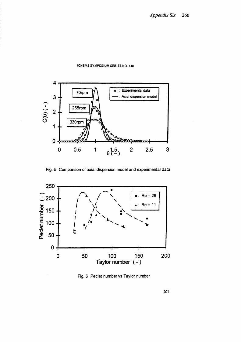
Appendix Six 260
ICHEME SY M PO SIU M S E R I E S NO. 14 0
o ; Experimental data
— : Axial dispersion model70rpm
I 265rpm2 --
C D
o 330rpm
30.5 21 t 2.5
Fig. 5 Comparison of axial dispersion model and experimental data
250■ : Re = 26•200
100 - -
200150100Taylor number ( -')
Fig. 6 Peclet num ber vs Taylor num ber
201
Appendix Six 261
Papers PublishedSamson S. S. Yim and P. Ayazi Shamlou, 1996. The Effect of Geometry On Mixing Performance In Continuous Couene-flow Devices. Proceedings: 5th World Congress Of Chemical Engineering. 1, 647-652.
The Effect of Geometry on Mixing Performance in Continuous Couette-Flow DevicesS. s. Yim Samson and P. Ayazi ShamlouChemical and Biochemical Engineering, University College London, Loncon WCIE 7]E
Abstract
Experimental results are reported on the residence time distribution (RTD) for Newtonian liquids in a continuous Couette-flow device. The effects o f rotational speed, axial fiowrate and the design o f inner rotating shafts are examined using stimulus-response technique. An axial dispersion model is used to describe the RTD dfM The results suggest significant variations fi*om plug fiow conditions depending upon the geometry of inner rotating design and the operating parameters.
The production and processing of viscous materials fi-equently involve the fiow of material through rotating devices. Examples include émulsification, polymerisation, solvent extraction, crystallisation, mixing and heat transfer operations (1,2,3,4). A continuous Couette-flow device consisting o f a stationary outer shell and a rotating inner cylinder with and without blades and wipers is firquently used in these operations because of its ability to promote good radial mixing and negligible axial dispersion (1,5). However, the mixing performance in these devices is afiected by the behaviour of the material during fiow and in the case o f steady state continuous processes a key foctor is the variation in the duration of stay within the process equipment experienced by "particles' which entered the equipment at the same time. In solvent extraction applications, for example, deviation fit)m plug fiow can result in a significant reduction in the mass transfer driving forces and thus the separation efficiency of the equipment can be detrimentally afiected (6). This variation is normally expressed in terms o f the residence time distribution (RTD) and as a result measurement and analysis o f RTD has become an important tool in the study o f continuous processes. Understanding the interaction between the RTD and process parameters in a continuous Couette-flow device is therefore o f basic research interest to academics and industrialists.
Experimental Detail and Methods
All the experiments reported in this study were carried out in a 1 m long horizontal coaxial cylinder device which is shown in Figure 1. The outer shell was fobricated from Perspex to allow visual observations of the fiow structure and had an inner diameter of 90 mm. Figure 2 shows the two different designs of the inner rotating shafts (SI and S2) used in this study and their specifications respectively. Both of the inner shafts were constructed from a stainless steel tube having an outside diameter of 76 mm and driven by a variable speed electric motor. The outer shell was equipped with two conductivity probes and a single injection point. Two probes, with platinum wire electrodes, were separated 400 mm apart in a horizontal line with the first probe positioned 200 mm from the injection point. The tracer solution was prepared fi’om concentrated KCl and the working liquid. The data from both conductivity probes were stored in a data acquisition system for analysis.
647
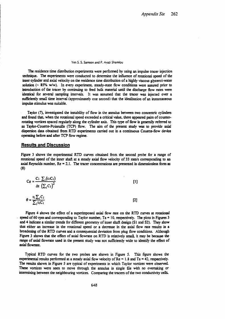
Appendix Six 262
Yim S. S. Sam son an d P. Ayazi Sham lou
The residence time distribution experiments were performed by using an impulse tracer injection technique. The experiments were conducted to determine the influence of rotational speed o f the inner cylinder and axial velocity on the residence time distribution o f a highly viscous glycerol-water solution (~ 85% w/w). In every experiment, steady-state flow conditions were assured prior to introduction o f the tracer by continuing to feed bulk material until the discharge flow rates were identical for several sampling intervals. It was assumed that the tracer was injected over a sufBciently small time interval (approximately one second) that the idealisation of an instantaneous inçulse stimulus was suitable.
Taylor (7), investigated the instability o f flow in the annulus between two concentric cylinders and found that when the rotational speed exceeded a critical value, there appeared pairs of counter- rotating vortices spaced regularly along the cylinder axis. This type o f flow is generally referred to as T^for-Couette-Poiseuille (TCP) flow. The aim of the present study was to provide axial dispersion data obtained from RTD experiments carried out in a continuous Couette-flow device operating before and after TCP flow regime.
Results and Discussion
Figure 3 shows the experimental RTD curves obtained from the second probe for a range of rotational speed o f the inner shaft at a steady axial flow velocity o f 33 mm/s corresponding to an axial Reynolds number. Re = 2.1. The tracer concentrations are presented in dimensionless form as (8)
Cl Si(tiCi)At (ZiCi)'
c b = J [1]
Figure 4 shows the effect of a superimposed axial flow rate on the RTD curves at rotational speed o f 60 rpm and corresponding to Taylor number. Ta = 10, respectively. The plots in Figures 3 and 4 indicate a similar trends for different geometry o f inner shaft design (SI and S2). They show that either an increase in the rotational speed or a decrease in the axial fiow rate results in a broadening o f the RTD curves and a consequential deviation from plug fiow conditions. Although Figure 3 shows that the effea of axial fiowrate on RTD is relatively small it may be because the range of axial fiowrate used in the present study was not sufficiently wide to identify the effect of axial fiowrate.
Typical RTD curves for the two probes are shown in Figure 5. This figure shows the experimental results performed at a steady axial flow velocity of Re = 1.8 and Ta = 42, respectively. The results shown in Figure 5 are typical o f experiments in which Taylor vortices were observed. These vortices were seen to move through the annulus in single file with no overtaking or intermixing between the neighbouring vortices. Comparing the tracers o f the two conductivity cells.
648
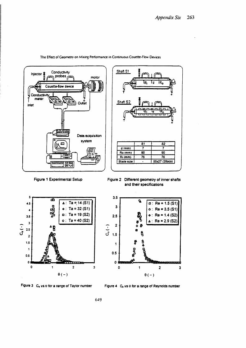
Appendix Six 263
T he Effect o f G eom etry on Mixing Perform ance in C ontinuous C ouette-F low D evices
Couette-now device
Conductivity I meter
Inlet0>W\Ci.\0V»
Data acquisition system
Figure 1 Experimental Setup
Shaft 81
t
Shaft S2
tfii Td IRo
J p j i n ,\ nmnirir~irnn I
"HT
S t S 2d I m m ) 7 7
R o i m m ) 9 0 9 0R i ( m m ) 7 6 7 6
B l a d e s i z e - 55x27 (280CS)
Figure 2 Different geometry of inner shafts and their specifications
a : Ta = 14 (81) o; Ta = 32 (31) D : Ta = 19 (82) o ; Ta = 40 (82)
0(- )
Figure 3 Ce vs 0 for a range of Taylor number
3.5Re = 1.5 (81) Re = 3.5 (81) Re = 1.4 (82) Re = 2.9 (82)
2.5
d
0.5
0 21 3
6(-)
Figure 4 0» vs e for a range of Reynolds number
649
Appendix Six 264
Yim S. S. Sam son an d P. Ayazi Sham lou
no appreciable difference could be seen in the shape of response curves except for a phase shift caused fy the distance-velocity lag.
For the experiments carried out in the present investigation a pulse was injected into the gap at an arbitrary time, t = 0. Following the injection, the tracer its concentration was measured at two positions in the gq>. These are the boundary conditions that describe an open-open system and the partial differential equation of the dispersion concerned with a pulse measurement technique in this type o f system has been solved analytically (8). The dimensionless tracer concentration. Ce, at the measuring point for the prevailing conditions is given by (8)
_ [Pe Pe ( i - e r4 6 [3]
where the dimensionless Peclet number, Pe is defined as
P . - ^ [4]
When Pe tends to infinity, the dispersion rate is negligible con^ared to the convection rate. The flow is defined as plug flow. However, wdien Pe approaches zero the comection rate is much slower that the dispersion rate and the flow is completely mixed.
Figure 6 shows that the comparison between experimental results and the axial dispersion model The agreement of the experimental tracer RTD curves for the liquid in the gap with Equation [3] is satisfactory. Equation [4] was used to obtain the individual longitudinal dispersion coefficietn, Q, ty fitting the observed time variation of the tracer concentration at the two probe positions.
The Peclet number was also evaluated by using the variance difference of the tracer response curves (1,2). The effect of rotational speed, expressed as Taylor number, on the Pe, is shown in Figure 7 for three axial flow rates expressed as Reynolds nunmer. When the speed of rotation o f the inner cylinder is zero, the flow regime in the aimular gap is laminar for both shafts SI and S2, a fiilfy developed laminar liquid velocity profile exists in the gap giving a high value of Pe. As the speed of rotation is slowly increased, the fluid flow become unstable and the Pe number decreases. For shaft SI, Taylor vortices develop causing an increase in the Peclet number again and a narrowdng o f the RTD curves. The maximum points in the figure (highest Pe) shown in Figure 7 correspond to the conditions at which the Taylor vortices are fully established along the cohunn and flow approaches near plug flow condition. With further increase in the speed of rotation of the inner cylinder intermixing and exchange o f material occurs at the boundaries between the neighbouring vortices causing an increase in the axial dispersion and a broadening of the RTD curves, and hence a decrease in the value o f Pe is observed as flow becomes increasingly turbulent with shaft S2. Figure 8 suggest that the introduction of blades on the inner shaft promotes the occurrence of turbulent flow and TCP flow could not be detected.
650
Appendix Six 265
T h e Effect o f G eom etry on Mixing Perform ance in C ontinuous C ouette-F iow D evices
Ta *42 : Re* 1.4.5
1st Probe I 2nd Probe3.5
U 2.5
0.5
10 20 30 40 50 600
□ : Expenmental data — : Axial dtspeision model
4.5
3.6iTa * 0
u 2.5Ta* 13
1.5ITa * 26
0.5
32.51.5 20.5 10t(s) 0 ( - )
Figures RTD curves for the two probes Figure 6 Comparison between experimental dataand axial dispersion model
400
Re = 1.4
Re = 1.8300
Re* 1.9
c 200
I100
100806040200
400
Re = 2.0
Re = 2.3300
-o -R e = 2.9
I 200
100
3020100Taylor number ( - ) Taylor number ( - )
Figure 7 Peclet number vs Taylor numberfor shaft SI
Figure 8 Peclet number vs Taylor number for shaft 32
651
Appendix Six 266
Yim S. S. Samson and P. Ayazi Shamlou
The data in Figure 7 were supported by visual observations o f the flow structure in the annulus Wiich indicated the presence of small vortices. These vortices first appeared in the region close to the walls of the inner rotating cylinder and gradually grew radially outwards until they reached the inner walls o f the outer shell (9). Unfortunately, a tten ^ to photograph these vortices have so 6 r seen unsuccessful
Conclusions
The RTD results were described by using an a single parameter axial dispersion model The results showed that the RTD was strongly dependent upon the geometry o f inner rotating device the operating parameters including rotational speed. The results also indicated that the width o f RTD narrowed only for shaft SI when the transition of flow from laminar to Taylor-Couette-PoiseuiHe regime over a range o f rotational speed. For shaft S2, it never show the occurrence o f TCP flow regime.
Nomenclature
C = Concentration (molL*')Ce = Dimensionless concentration (-)d = Annular gap (L)D » Axial dispersion coeflScient ( L ^ ‘)L = Distance between two probes (L)N = Rotation speed (T ‘)Pe = Peclet number ( - )R , Ro = Radius o f the inner and outer cylinder (L'')Re = Reynolds number = 2dv/v ( - )t =Time(T)Ta = Taylor number = (2:iN)Ro*^d^ /v ( - )V = Aj flow velocity (LT*)6 = Dimensionless time ( - )V = Kinematic viscosity ( L ^ ‘)
References
1. Kataoka, K., DoL H., Hongo, T. and Futagawa, M.,J. Chem. Engng Japan, 8:472-476 (1975).2. Pudjiono, PJ., Tavare, N.S., Garside, J. and Nigam, K.D.P.,CAem. Engng J., 48:101-110(1992).3. Abichandani H. and Sarma, S.C., Chem. Engng Sci, 43:871-881(1988).4. Daongaonkar, K.R., Pratt, H.R.C. and Steven, G. W., AIChE J., 37:694-704 (1991).5. Legrand, J. and Coeuret, F., Chem. Engng ScL, 41:47-53 (1986).6. von stockar, U. and Lu, X., Ind. Engng Chem. Res., 30:1248-1257 (1991).7. Taylor, G. I., Phil. Trans., A233:289-343 (1923).8. Levenspiel 0 ., Chemical Reaction Engineering, Wiley, New York, Chapter IX (1965).9. Ogawa, A., Fujita, V. and Nagabayashi N., Chem. Engng Commun., 37:209-222 (1985).
652
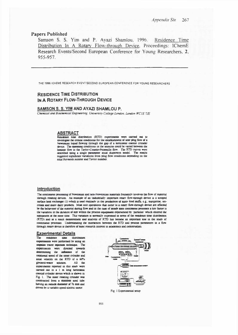
Appendix Six 267
Papers PublishedSamson S. S. Yim and P. Ayazi Shamlou, 1996. Residence Time Distribution In A Rotary Flow-through Device. Proceedings: IChemE Research Events/Second European Conference for Young Researchers, 2, 955-957.
THE 1 9 9 6 ICHEME RESEARCH E V EN T/SEC O N D E U R O PE A N CO NFERENCE FOR YOUNG R E SEA R C H E R S
R E S ID E N C E TIM E D ISTR IB U TIO N
IN A R o t a r y F l o w - T h r o u g h D e v i c e
S A M S O N s . s . YIM A N D A Y A ZI S H A M L O U P .Chemcal and Biochemcol Engineering. University College London. London WCIE 7JE
A B S T R A C TReadcnoc tune dmnbotioD (RTD) experunents woe caried oat to investigate the critical oondiaons for the estabiisfament <tf tiear ping fknv of a Newtonian ixghd flowing through the gap of a bonzontal coaxial cylinder device. The npwanng condmons in the annulus could be varied between the laminaT flow 10 the TayiorCouette"fQiseaille flow The RTD carves were described «mg a s tn ^ axial dispersion model The resultsQiggffOfri ngmflcant variations from plug flow conditions depending on the axial Revnolds number and Tavlor number.
I n t r o d u c t i o nThe continuous processing of Newtonian and non-Newtonian materials frequently involves the flow of material through rotating devices. An «jnipi*? of an indnsmaliy unporum rotary flow-through device is a scraped surface heat prrhawgw (i) which is used routinely in the production of many food stuffr e.g., margarine, icecream and many dairy prnfocts. Most unit operations that occur m a rotary flow-through device are affected by the behavMur of the material during fiow and tn the case of steady gate comumoui processes a key factor is the variation m the duration of stay within the process wpnpw«<tit experienced by ‘parades’ which entered the mynpwwn, g the ame time. This Variation is normally expressed in terms of the residence ttme distnbtmon (RTD) and as a result measuremem and analysis of RTD has became an unponam tool in the study of coniinnoas processes. Understanding the interaction between the RTD and process parametos m a flow through rotary device IS therefore of basic research interest to academics and industnaiists.
E x p e r im e n ta l D e ta i l sThe residence nmg distribution
were performed by usmg an imppiq» tncet tiymrm techtuqoe. The
jiinfnn were directed towards determining the iwWu nr of the rotatimal speed of the umer cylinder and axial velocity on the RTD of a 60% glycerol-water solution. All the « p eiiments reported tn this study were earned out m a 1 m long honzomal coaxial cylinder device which u shown m Fig. 1. The mner rotating cybnder was constructed from a ged tubehaving an outside of 76 anddriven by a variable speed electnc motor.
Fig 1 Expenmental setup
955
Appendix Six 268
THE 1 9 9 6 ICHEME RESEARCH EVENT/SECOND EUROPEAN CONFERENCE FOR YOUNG RESEARCHERS
The Older f h e l l was f a h n r a tn r i from Ptispcji ID allow visual observauoss of the How strocmre and had an m n w
ihwm^i-T of 90 mm. The outer shell was equipped with two conductivity probes and a single mjecoon poinl Two probes, with ptatiimm wire dectiodes. were tepaiated 400 mm apart in a honzomal line with the first probe poeitiooed 200 mm fiom the mjecoon poinL The tracer sohmon was prepared from concwmated KQ and the working liquid. The data fiom both oooductivity probes were stored m a dau acqmsmon system fiir analysis.
Results and DiscussionTypical RTD curves for the two probes are shown in Fig. 2 This figure shows the expenmental results performed at a steady axial fiow velocity of 20 mm/s and at a rotational speed of 110 rpm oonespondtng to an asal Reynolds number. Re ■ 24.7 and Taylor number. Ta - 121. respecnveiy.
For the experiments earned out m the present investi ganon a pulse was mjeaed into the gap at an arbitrary tfine, t « 0. Following the tracer, its oonceatiauon was mei stired at two positions m the gq>. These are the boundary condmons that describe an opennipen system and the partial difEdenaal rqnannn of the dispersioo concerned with a pulse measurement «fhnwpp in this type of system has been solved analytically (2). The dùnensiooless tracer onrwiiTration, C*. at the measanng pomt for the prevailing conditions is given by (2)
Cf = (Pe / 4 ie^ ' : cxp(-Pe(l - / 4 ^ (IJ
where the thmensuailess Pedet number. Pe is defined as
Pe-vU D (2J
When Pt tends to infinity, the dispersion rate is negligible compared to the convection rate. The flow is «tiHÿiwuri as plug flow. However, when Pe approaches zero the comecoon rate is nmch slower that the (hspersioo rate and the flow is completely mixed.
Fignre 3 shows that the comparison between expenmental results and the axial dispersion model The agreemem of the «TyrmKnwai nacer RTD curves for the liquid m the gap with Eq [I] is saosfsctory. Equation [2] was used to obtam the individnal longrtudinal dispersion cntrffirimt D. bv fttnng the observed time variation of the tracer conoemration at the two probe posmons.
The Pedet muntaer was also evaluated by usmg the varunce difference of the tracer response curves (3.4). The effed of rotaoooal speed, expressed as Taylor number, on the Pe. is shown m Fig 4 for two axial flow rates eoqaessed as Reynolds nmnber. When the speed ctf rotauon of the mner cybnder is low. the flow regime in the «itmiar gap g lamnar (Couette) flow. a fully developed laminar liquid vdocity profile exists m the gap giving a low value of Pe. As the speed of rotanon is slowly increased. Taylor vortices develop ransmg a gradual m the «tmI dispersion and a narrowing of the RTD curves The mammmw points m the data(highest Pe) shown in Fig 4 correspond to the conditions at which the Taylor vortices are fully established along the column and flow near plug flow condmoa With further increase m the speed of rotationof the inner cylinder intermixing and exchange of material occurs at the boundaries between the neighbouring vortices «n«ng an increase m the axial ch^rrsion and a broadetung of the RTD curves, and hence a decrease m the value of Pe IS observed.
The data in Fig 4 were supported tw visual observations of the flow structure m the annulas which inAtcateA the presence of flow mstabüity in the form of small vortioes These vortices first appeared m the region close to the walls cS the mner rotating cylinder and gradually grew radially outwards until they reached the inner walls of the outer shell The buth and growth of the Taylor vomces occurred over a penod of time and a range of speed dependmg on the axrai flow rate In the presem studv . the cnucai speed at which the Pe had Its maximum value was considered arbitranly to represent the condmons at which the Taylor vortices were fully formed
The critical Taylor number. Ta., necessary for the estahlishmeni of Taylor voraces plotted against the nperaiing axial Reynolds is shown m Fig S. The change m the cnucai Tavior number. Ta., with axial Reynolds number follow the trend reported bv previous groups which are also shown. These plots suggest that the cnucai Taylor «nmivr |$ a function of the dimensionless gap as well as the axial Revnolds number.
956
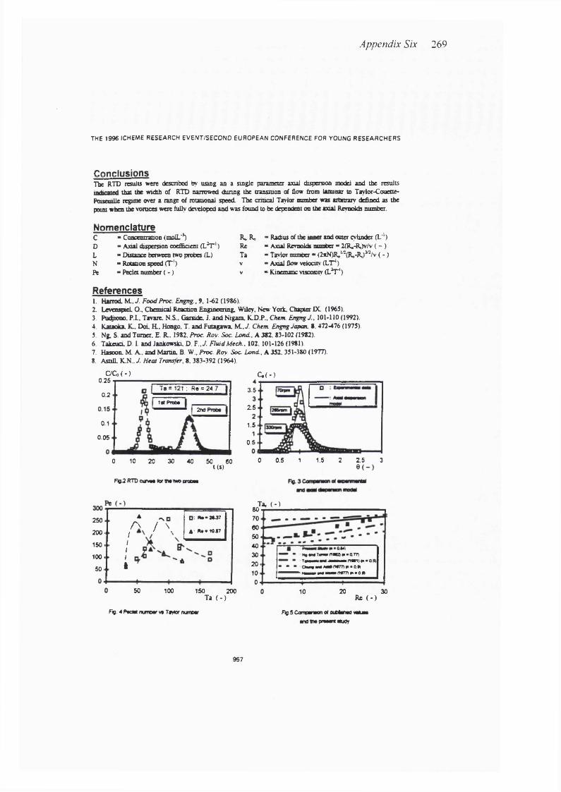
Appendix Six 269
THE 1 9 9 6 ICHEME RESEARCH E V E N T /SE C O N D EU RO PEA N CONFERENCE FOR YOUNG R E SE A R C H E R S
C o n c l u s i o n sThe RTD resulu were descnbed by usmg an a smgie paiameter axial dispenmn model and the results
that tfac Width of RTD nanowed dunng the transmon of flow flom laminar to Taylor-Couene- Potsenille ttgune over a range of rotational speed. The critical Taylor nmnber was artanrary defined as the point when the vomces were fully dei'eloped and was found to be deprnrtrnt on the axial Reynolds number
N o m e n c la tu r eC - ConoemxaQon (molL'^ R. R«D ” Axial dispersion coeffiaent ( L ^ ') ReL " Distance between two probes (L) TaN -Rotanon speed (T ‘) vPe - Peclet number ( - ) v
- Radius of the mwer and outer cylinder (L'') » Axial Revnolds number - 2(R.-Rjv/v ( - )- Tayiw number - (2*N)Re*'’(Ro-RJ^/v ( - ) « Axial flow vekxaty (LT*)- Kinematic viscosity ( L ^ )
R e f e r e n c e s1. Harrod. \L ,J . Food Proc. Engng., 9. 1-62 (1986).2. LevenspieL O.. Chemical Reaction Engineering, Wiley, New York. Chapter DC (1965).3. PD(^ono.P.L, Tavare. N.S.. Garside. J. and Nigam. K.DJ>.,CAeffl. Engng y., 101-110(1992). 4 Kataoka. K. Dot. R . Hongo, T. and Futagawa. h/L,J. Chem. Engng Japan, S. 472-476 (1975).5. Ng, S. and Turner, E R.. 1982. Proc. Roy. Soc. Lond, A 382. 83-102 (1982).6. Takeuci. D. L and Jankowski. D. P., J. Fluid Mech., 102.101-126 (1981).7. Hasoon. M A . and Mamn, B. W., Proc. Roy. Soc. Lond, A 352. 351-380 (1977).8. AstilL K.N.. J. Heat Transfer, 8, 383-392 (1964).
C/Co(->0 .2 5
Ta = 121 ; R* = 24.70.2
1st Prêt»2nd
0.1
0.05
0 10 20 30 40 50 60t(S)
Fip2 RTD cunwa tor tha IWD prabaa
250.
200.>
/150. /
1100. 150. I
AA / " \
o na-atar A: R«>10J7
'A
50 100 150 200Ta ( - )
np. 4 Padat marmar va Ta>«or nunear
C .(-)
3.5
25
1.5
0.5
0 0.5 1.5 2 25 31
80706050403020100
Ta. ( - )
M| ■» T««v naa w ■ ar?) tmh- JMM» naai) «I ■ 0 s) OM» M MM narr) «I ■ aw
■>■11»—«MMoarnu-aw
10 20 30Re ( - )
Fi05 Companaen et neawM d >mtuaa
and ma praaam study
957
Appendix Six 270
Papers PublishedSamson S. S. Yim and P. Ayazi Shamlou, 1996. Residence Time Distribution (RTD) In A Rotan' Flow-through Device with non-Newtonian Fluids. AlChE Annual Meeting (Oral presentation and full paper).
R e s i d e n c e T im e D i s t r i b u t i o n ( R T D ) In A R o t a r y F l o w - t h r o u g h D e v i c e W it h
N o n - N e w t o n i a n F l u id s
SAMSON S. S. YIM AND AYAZI SHAMLOU P.Chemical and Biochemical Engineering, University College London, London WCIE 7JE
ABSTRACT
The flow in the gap of a pair of rotating cylinders with and without superimposed axial flow has many potential applications in situations where good radial mixing and negligible axial dispersion are required. In the present study, RTD experimental data are reported for Non-Newtonian liquids flowing in the gap between two horizontal coaxial cylinders in the presence of a small superimposed axial flow. Liquid motion was achieved by the rotation of the inner cylinder and the action of a pump which allowed independent control of the axial flow in the gap. The RTD curves were described using an axial dispersion model and the experimental data were interpreted in terms of a Peclet number. The data were used to identify the critical Taylor number at or close to the point when flow changed from Couette to Couette-Taylor flow regime. The analysis showed that significant variation from plug flow occurred as the flow approached the point of criticality.
MATERIALS AND METHODS
The RTD data were obtained by using an impulse tracer injection technique. The experiments were carried out in a 1 m long horizontal coaxial cylinder device (Figure 1). The inner cylinder had a diameter o f 76 mm and driven by a variable speed electric motor. The outer shell, with an diameter of 90 mm, was equipped with two conductivity probes. 400 mm apart, and a single injection point. The tracer solution was prepared from concentrated KCl and the working liquid. The fluids employed in this study were various concentrations of CMC and Xanthan gum (X-gum) solutions (see Table 1).
RESULTS AND DISCUSSION
Typical RTD curves for the two probes at a low axial flow rate are shown in Figure 2. The data were analysed in terms of a single parameter axial dispersion model used previously by the authors to describe the flow of Newtonian liquids in the same device [1]. Thus, the dimensionless tracer concentration. C©, at the measuring point is given by [2]
C e = ( P c / 4 7 1 0 ) '^ 2 e x p [ - P e ( I - 0 ) ’ /40] ( 1 )
where the dimensionless Peclet number, Pe = vLD, was evaluated by using the variance difference of the two tracer response curves. The agreement between the predictions by the dispersion model and the experimental data is satisfactory as shown in Figure 3.
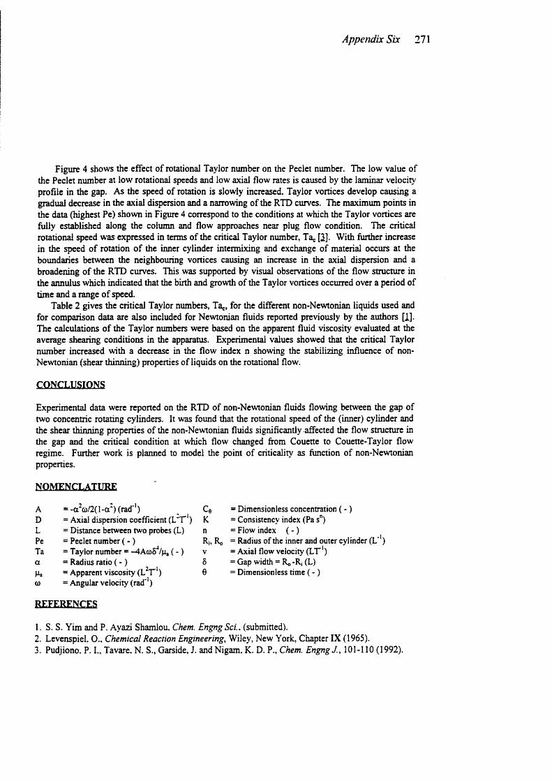
Appendix Six 271
Figure 4 shows the effect of rotational Taylor number on the Peclet number. The low value of the Peclet number at low rotational speeds and low axial flow rates is caused by the laminar velocity profile in the gap. As the speed of rotation is slowly increased, Taylor vortices develop causing a gradual decrease in the axial dispersion and a narrowing of the RTD curves. The maximum points in the data (highest Pe) shown in Figure 4 correspond to the conditions at which the Taylor vortices are fully established along the column and flow approaches near plug flow condition. The critical rotational speed was expressed in terms of the critical Taylor number, Ta [1]. With further increase in the speed of rotation of the inner cylinder intermixing and exchange of material occurs at the boundaries between the neighbouring vortices causing an increase in the axial dispersion and a broadening of the RTD curves. This was supported by visual observations of the flow structure in the annulus which indicated that the birth and growth of the Taylor vortices occurred over a period of time and a range of speed.
Table 2 gives the critical Taylor numbers, Ta^ for the different non-Newtonian liquids used and for comparison data are also included for Newtonian fluids reported previously by the authors [1]. The calculations of the Taylor numbers were based on the apparent fluid viscosity evaluated at the average shearing conditions in the apparatus. Experimental values showed that the critical Taylor number increased with a decrease in the flow index n showing the stabilizing influence of non- Newtonian (shear thinning) properties of liquids on the rotational flow.
CONCLUSIONS
Experimental data were reported on the RTD of non-Newtonian fluids flowing between the gap of two concentric rotating cylinders. It was found that the rotational speed of the (inner) cylinder and the shear thinning properties of the non-Newtonian fluids significantly affected the flow structure in the gap and the critical condition at which flow changed from Couette to Couette-Taylor flow regime. Further work is planned to model the point of criticality as function of non-Newtonian properties.
NOMENCLATURE
A = -a^û)/2(l-a‘) (rad"') Ce = Dimensionless concentration ( - )D = Axial dispersion coefficient (L 'T ') K = Consistency index (Pa s")L = Distance between two probes (L) n = Flow index ( - )Pe = Peclet number ( - ) Ri, Ro = Radius of the inner and outer cylinder (L '')Ta = Taylor number = -4A(o6'*/|ia ( - ) v = Axial flow velocity (L T ')a = Radius ratio ( - ) Ô = Gap width = Rg -Rj (L)
= Apparent viscosity (L^T ') e = Dimensionless time ( - )(0 = Angular velocity (rad ')
REFERENCES
1. S. S. Yim and P. Ayazi Shamlou. Chem. Engng Sci.. (submitted).2. Levenspiel, 0 ., Chemical Reaction Engineering, Wiley, New York, Chapter IX (1965).3. Pudjiono. P. I., Tavare. N. S., Garside, J. and Nigam, K. D. P., Chem. Engng J., 101-110 (1992).
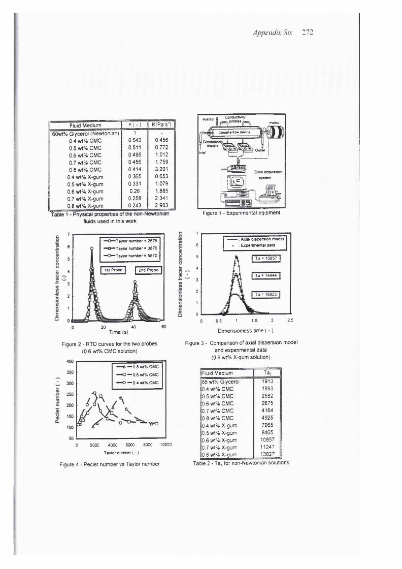
Appendix Six 272
Fluid Medium n ( - ) K(Pa s")
60wt% Glycerol (N ew tonian) 1 -
0.4 w t% CMC 0.543 0.456
0.5 wt% CMC 0.511 0.772
0.6 wt% CMC 0.495 1.012
0.7 wt% CMC 0.456 1.759
0.8 wt% CMC 0.414 3.201
0.4 w t% X-gum 0.365 0.653
0.5 w t% X-gum 0.331 1.079
0.6 wt% X-gum 0.26 1.885
0.7 wt% X-gum 0.258 2.341
0.8 w t% X-gum 0.243 2 .903
fluids u se d In this work
—O —Taylof number * 2675
Taykx number * 3876
- O —Taylor number * 5870
2nd Probe1st Probe
20 40Tim e (s)
Figure 2 - RTD cu rv es for the two p robes (0.6 wt% CMC solution)
— 0.8 wt'/oCMC
1— 0 6 wt%CMC
' — 0 4wt%CMC
TTO
m otor
Couette-flow device
OutletInlet
C3
Figure 1 - Expenm ental eq ipm en t
7— : Axial dispersion model . ; Expenmental data6
Ta = 10857 |5
4
Ta = 149443
2Ta = 18923 |
10
0.5 1 1.5 2
D im ensionless tim e ( - )
2.5
Figure 3 - C om parison of axial d ispersion m odel and experim ental d a ta
(0.6 wt% X-gum solution)
2000 4000 6000 8000 10000
Taylor number ( - )
Fluid M edium Ta,
85 wt% Glycerol 1913
0.4 wt% CMC 1993
0.5 wt% CMC 2582
0.6 wt% CMC 2675
0.7 wt% CMC 4164
0.8 wt% CMC 4925
0.4 wt% X-gum 7065
0.5 wt% X-gum 8465
0.6 wt% X-gum 10857
0.7 wt% X-gum 11247
0.8 wt% X-gum 13827
Figure 4 - P ec le t num b er vs Taylor num ber Table 2 - Ta^ for non-N ew tonian solutions
Appendix Six 273
Papers AcceptedSamson S. S. Yim , N. Titchener-Hooker and P. Ayazi Shamlou, 1997. Prediction of Critical Tavlor Number For Non-Newtonian Fluids. The First European Congress on Chemical Engineering.
P r e d i c t i o n O f C r i t i c a l T a y l o r N u m b e r In C o u e t t e F l o w
F o r N o n - N e w t o n i a n F l u id s
S A M S O N s . s . y im , N . T IT C H E N E R -H O O K E R A N D P . AYAZI S H A M L O U
Chemical and Biochemical Engineering, University College London, London WCIE 7JE
ABSTRACT
A numerical method is presented for solving the eigenvalue problem which governs the stability o f non-Newtonian liquids in Couette flow. The method is particularly useful in obtaining the eigenfunctions associated with various modes o f instability. Consideration is given to the cases of radius ratio from 0.1 to 0.99 and the non-Newtonian flow index from 0.2 to 1. The Taylor number, being a criterion of the stability, has been defined using the mean q^parcnt viscosity. Results showed that the critical value o f Taylor number Ta« was an increased as either the flow index or radius ratio increased.
INTRODUCTION
Couette flow describes the steady circular flow o f a liquid contained between two concentric rotating cylinders. The parameters usually used to specify the flow are the radius ratio, a (=Ri/R2), angular speed ratio, |3 (=Q2/Qi) and the Taylor number. Ta, which is a non- dimensional measure o f the gradient of centrifugal force. G. I. Taylor (1923) provided the first experimental and theoretical evidence on the breakdown o f a Newtonian liquid in Couette flow with increasing speed o f rotation of the cylinders, in which the laminar fiow would be replaced by a cellular pattern around the cylinders in layers o f vortices - now known as Taylor vortices - (see Figure 1). The instability of Couette flow has since been studied by a number o f workers yielding a vast amount o f information on the hydrodynamics (Chandrasekhar, 1961) and applications o f Taylor-Couette flow (Cohen and Marom, 1983). In the present study, a more general Couette fiow instability problem will be investigated to include the effect of non-Newtonian properties on onset o f fiow instability.
THEORY
Consider an inconçressible non-Newtonian liquid fiow between two infinitely long concentric cylinders in the usual cylindrical co-ordinates r, 6, z (See Figure 1). If we denote the radial, tangential and axial velocity components respectively by u,, ue and Uz, and the pressure by p, the Navier-Stokes equations give an exact time-independent solution of the form
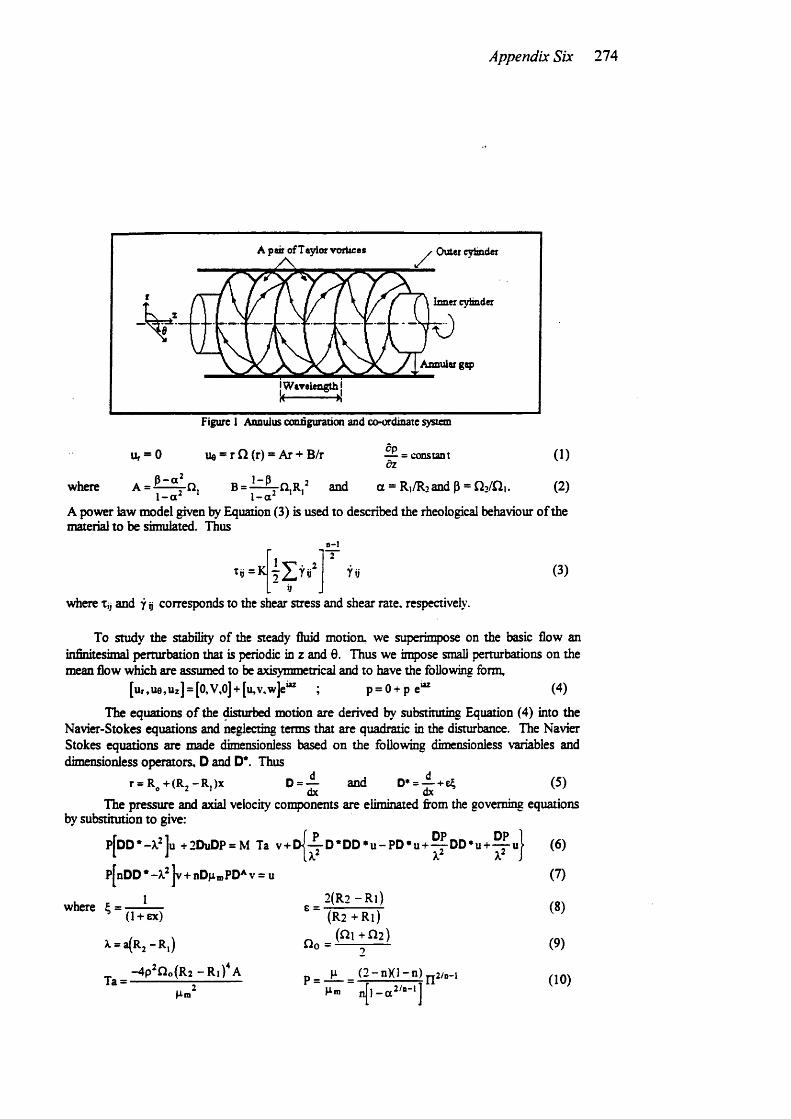
Appendix Six 274
A p a ir o f T a y lo r v o rL c e a O u te r c y l in d e r
A n n u la r g q )
I W a v e le n g t h I
where
U r = 0
p-a^
Figure 1 Annulus conâguration and co-ordinate system
U e = rQ (r) = Ar + B/r ^ = constant
A =
ÔZ
and a = R1/R2 and P =
(1)
(2)1-a ' 1-aA power law model given by Equation (3) is used to described the rheological behaviour o f the material to be simulated. Thus
0 -1
Xii =K
where tÿ and ÿij corresponds to the shear stress and shear rate, respectively
Yü (3)
To study the stability of the steady fhiid motiotL we superimpose on the basic flow an infinitesimal perturbation that is periodic in z and 6 . Thus we inqx)se small perturbations on the mean fiow which are assumed to be axisymmetrical and to have the following form,
[ u r , U 0 , U z ] = [O,V,O] + [u,v,w]e'“ ; p = 0 + p e “ (4)
The equations o f the disturbed motion are derived by substituting Equation (4) into the Navier-Stokes equations and neglecting terms that are quadratic in the disturbance. The Navier Stokes equations are made dimensionless based on the following dimensionless variables and dimensionless operators. D and D*. Thus
r = R + (R ,- R ,)x D = -^ and D* = -^ + e4 (5)dx dx
The pressure and axial velocity components are eliminated fi’om the governing equations by substitution to give:
p[dD*-X^1u +2DuDP = M Ta v + d| 4 -D * D D * u -P D * u + ^ D D * u + ^ iI J X
P nDD * -X^ jv+nDpmPD* v = u
2 ( R 2 - R i )where =(1 + ex)
X = a(R2 - R ,)
-4p ^n o (R 2 - R i ) V
e =
Qo =
(R2 +R i) (O1 +O2 )
Ta = P =Pm Pm
( 2 - n K l - n ) « 2/D-1
(6)
(7)
(8)
(9)
(10)
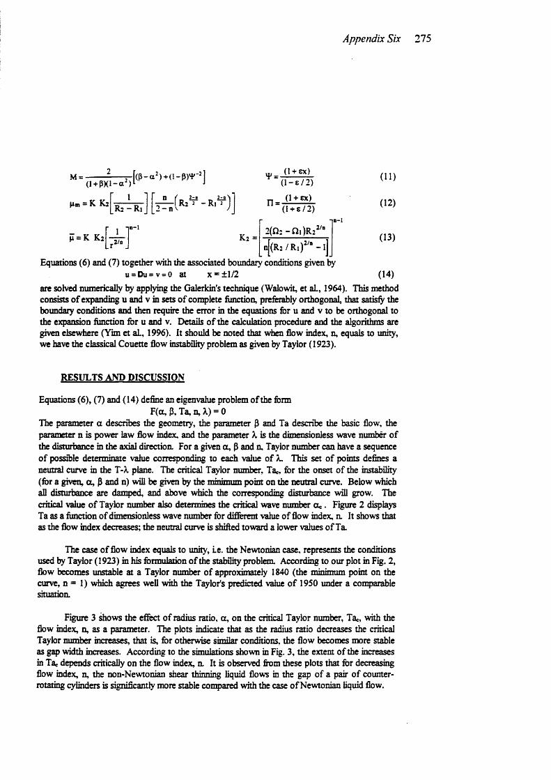
Appendix Six 275
M Y =
Pm = K*ü 1R2 - R 1
n=
(1-1-ex) ( l - e / 2 )
(1 + ex) (I + e / 2 )
p = K K2Lr 2/n
n—IK2 =
10-1
2(n:-0,)R2 2/n
( 1 1 )
( 12)
(13)
(14)are solved numerically by applying the Galerkin's technique (Walowit, et aL, 1964). This method consists o f expanding u and v in sets o f complete function, preferably orthogonal, that satisfy the boundary conditions and then require the error in the equations for u and v to be orthogonal to the expansion function for u and v. Details o f the calculation procedure and the algorithms are given elsewhere (Yim et aL, 1996). It should be noted that wbm flow index, n, equals to unity, we have the classical Couette flow instability problem as given by Taylor ( 1923).
n |(R j/R i)^ '- l]
Equations (6) and (7) together with the associated boundary conditions given by u = Du = v = o at X = ±1/2
RESULTS AND DISCUSSION
Equations (6), (7) and (14) define an eigenvalue problem of the formF(a, p. Ta, n, X) = 0
The parameter a describes the geometry, the parameter p and Ta describe the basic flow, the parameter n is power law flow index, and the parameter X is the dimensionless wave number o f the disturbance in the axial direction. For a given a, P and n, Taylor number can have a sequence of possible determinate value corresponding to each value of X. This set of points defines a neutral curve in the T-X plane. The critical T^lor number. Ta*, for the onset o f the instability (for a given, a , P and n) will be given by the minimum point on the neutral curve. Below which all disturbance are damped, and above which the corresponding disturbance will grow. The critical value o f Taylor number also determines the critical wave number a * . Figure 2 displays Ta as a function o f dimensionless wave number for different value of flow index, n. It shows that as the flow index decreases; the neutral curve is shifted toward a lower values o f Ta.
The case o f flow index equals to unity. Le. the Newtonian case, represents the conditions used by T^lor (1923) in his formulation o f the stability problem. According to our plot in Fig. 2, flow becomes unstable at a Taylor number of approximately 1840 (the minimum point on the curve, n = 1) which agrees well with the Taylor's predicted value o f 1950 under a conçarable situation.
Figure 3 shows the effect o f radius ratio, a, on the critical Taylor number, Ta*, with the flow index, n, as a parameter. The plots indicate that as the radius ratio decreases the critical Taylor number increases, that is, for otherwise similar conditions, the flow becomes more stable as gap width increases. According to the simulations shown in Fig. 3, the extent o f the increases in Tac depends critically on the flow index, n. It is observed fiom these plots that for decreasing flow index, n, the non-Newtonian shear thinning liquid flows in the gap of a pair o f counter- rotating cylinders is significantly more stable conpared with the case o f Newtonian liquid flow.
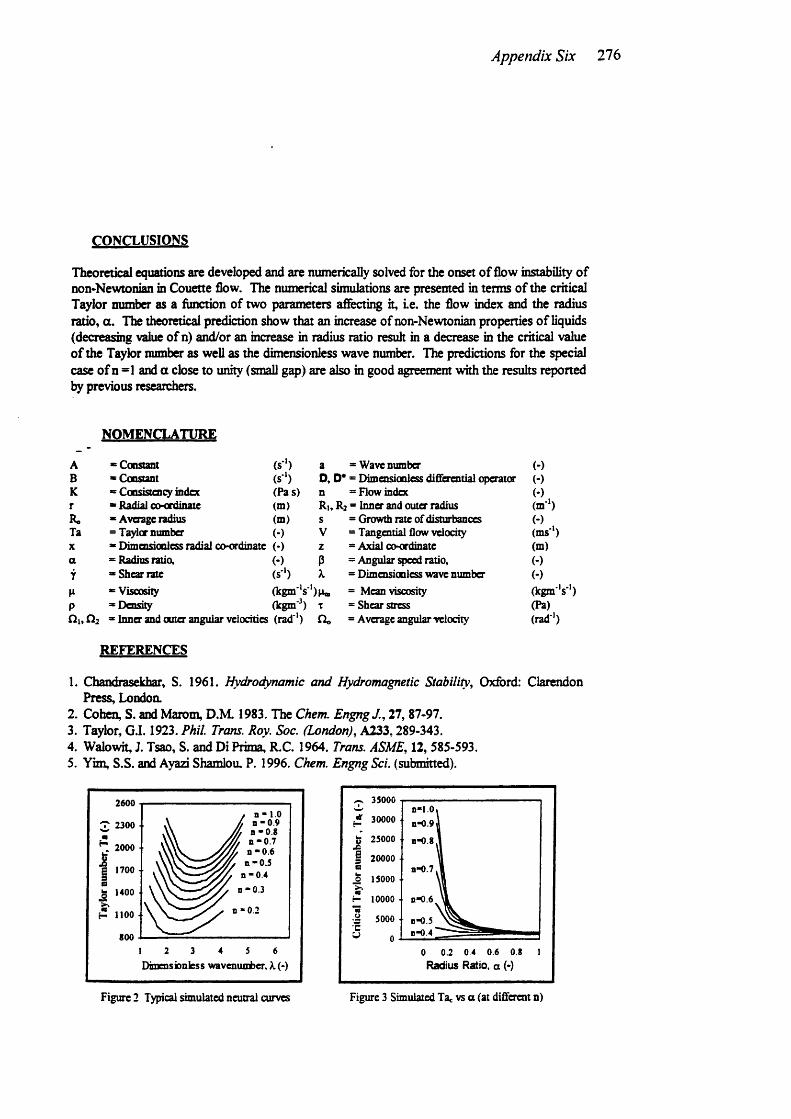
Appendix Six 276
CONCLUSIONS
Theoretical equations are developed and are numerically solved for the onset o f flow instability o f non-Newtonian in Couette flow. The numerical simulations are presented in terms o f the critical Taylor number as a function of two parameters affecting it. Le. the flow index and the radius ratio, a. The theoretical prediction show that an increase of non-Newtonian properties o f liquids (decreasing value o f n) and/or an increase in radius ratio result in a decrease in the critical value of the Taylor number as well as the dimensionless wave number. The predictions for the special case o f n =1 and a close to unity (small g ^ ) are also in good agreement with the results reported by previous researchers.
NOMENCLATURE
A s Constant (s ') a = Wave number (-)B * Constant (s ') D, D* = Dimensionless differential operatw (-)K = Consistency index (Pas) n = Flow index (•)r s Radial coKxdinate (m) Ri, Rj = Inner and outer radius (m ')R, - Average radius (m) s = Growth rate of disturbances (-)Ta = Ta)dQr number (-) V = Tangential flow velocity (ms')X » Dimensionless radial co-cxdinate (-) z = Axial co-ordinate (m)a = Radius ratio. (-) P = Angular qieed ratio. (-)f * Shear rate (s ') X = Dimensionless wave number (-)
“ Viscosity (kgm ''s')n„ = Mean viscosity (kgm's*')P “ Density (kgm 'l T = Shear stress (Pa)Qi, O] » Inner and outer angular velocities (rad ) a, = Average angular velocity (rad')
REFERENCES
1. Chandrasekhar, S. 1961. Hydrodynamic and Hydromagnetic Stability^ Oxford: Clarendon Press, London.
2. Cohen, S. andMarom, D.M 1983. The Chem. EngngJ., 27, 87-97.3. Taylor, G.1.1923. Phil Trans. Roy. Soc. (London), A233,289-343.4. Walowh, J. Tsao, S. and Di Prima, R.C. 1964. Trans. ASME, 12, 585-593.5. Yim, S.S. and Ayazi Shamlou. P. 1996. Chem. EngngSci. (submitted).
2600
T 2300 mT 2000
J 1400
H 1100
900
/ n - 1.0/ n - 0 9
Æ n -0 .8n -0 .7n -0 .6
D - 0 4. - 0 3
%1 2 3 4 5 6Dimensioniess wavenunter. A. (-)
^ 35000
£ 30000
25000
20000
^ 15000
H 10000
5000
Radius Ratio, a (-)
Figure 2 Typical simulated neutral curves Figure 3 Simulated Tac vs a (at different n)
Appendix Six 277
Papers AcceptedSamson S. S. Yim and P. Ayazi Shamlou, 1997. Prediction of Critical Tavlor Number in Rotating Flow-through Devices, Proceedings; 1997 Jubilee Research Events.
Prediction Of Critical Taylor Number In Rotating Flow-Through Devices
SAMSON s . s . YIM AND AYAZI SHAMLOU P.Chemical and Biochemical Engineering, University College London, London WCIE 7JE
ABSTRACTTheoredcal and experimental results are presented showing the effects of operating and geometrical parameters tm the transition of laminar to Taylw vortex flow for induced rotational-axial flow in the gap of a pair of rotating cylinders. The simulations indicated that annular rotational flow became more stable in the presence of a small d^ree of axial flow and as gap width increases. Limited experimental data also were provided on the residence time distribution for flow of Newtonian liquids through the gap of two rotating cylinders. The results were successfully analysed and assessed using the simulations studies.Keyword: Rotating flow-through devices, Navier-Stokes equations,
Taylor number, Tayira- vortex flow,Residence time distribution, Peclet number.
IntroductionThe rotational flow generated ly a pair of coaxial cylinders, especially with a small superimposed axial flow, can be used to manipulate the residence time distributicm (RTD) of various species in the gap in order to promote radial mixing with negligible axial dispersim (Kataoka et al., 1981), conditions that are considered prerequisite for good mass and beat transfa and (bio)chemical reactions in many process engineering operations. In these unit operations, the dependence of the RTD of the different species on the fluid flow field occurring in the annulus is of great oq>erimental and theoretical interests.
TheoryFor an incompressible Newtonian liquid flowing under laminar flow cmdition between two infinitely long concentric cylinders (qdindrical co-ordinates r, 8, z). The radiaL tangential and axial velocity components respectively hyu^ue and Uz, and the pressure, p, can be obtained uniquely from the Navier-Stokes equations.
Ur * 0
u. = = —
ue * r Q (r) * Ar + B/r
apdz
= constant
, P — ccwhere A = - —l-o/ '
1 +1-(R,/Rj)^hXRj/R,)
(1)
(2)
(3)
(4)
where a = Ri/Ri and P = Qj/Qi. (5)
To study the condition leading to the instability of the laminar modem, we superimposed on the basic flow an infinitesimal perturbation that was periodic in z and 6. The small perturbations imposed on the mean flow were assumed to be axisymmterical and to have the following form.
Appendix Six 278
[DD*+nju = Ta M v + D-^[D*D + n]
= ; p = 0 ^ p (6)
The equations of the disturbed motion were derived by substituting (6) and a similar expression for p into the Navier-Stokes equations, neglecting terms that were quadratic. The resulting equations were made dimensioaiess by using the following:
r = R + ( R , - R , ) x D = — and D* = — rc^ (7)° ' dx dx
The pressure, axial velocity component were eliminated by substituuon. reducing the number of cquatims as follows
D * u l Re(DF) i
— J-— ®[DD*+n]v = u (9)
wheren = i ( G - A f R e ) - % \ (10)
A , - R . fc X = a ( R , - R , ) (II)
v‘ v“
F = --------:----- :------- f(l-OL^)lnT + a ^ ( Y - l ) l n a | (14)( 1 - 0 ) + ( l + o ) ln a i J
Equaticms (8) and (9) together with the associated boundary conditions given by:
u = Du = v = 0 at X = ±1/2 (15)
were solved numerically by applying the Galerkin's technique (WalowiL et al., 1964). Details of the calculation procedure and the algorithms are given elsewhere (Yim et al., 1996) and arc only briefly outlined here. For a fixed flow rate (axial Reynolds number) and condition given by a , and fi, Eqs. (8) and (9) were solved to yield values of Taylor numbers for a range of values of the dimensionless wave number k and growth rate a.
Results and DiscussionThe residence time distribuiicm experiments were dircacd towards examming the eflfccts of axial flow rate, gap width and the speed of rotation on the RTD of a range of glyccrol-water solutions of different viscosities (Table 1). A general arrangement of the experimental sa-up is shown schematically in Figure 1. The expcnmems were performed under operating conditions that included the pomt of cnucality. Full details of the flow device and experimental procedure have been reported elsewhere (Yim, 1997).
Figure 2 shows typical simulated neutral curves for the case of zoo axial flow, a range of narrow gap (a =0.9 - 0.99) and speed ratio, P = 0. The minimum point on the neutral curve defines a critical value of the Taylor number, below which all disturbance arc damped, and above which the disturbance will grow to become vortices. Figure 3 shows the variation of the critical Taylor number as a function of the axial Reynolds number. From these plots it can be seen that for fixed a as the flow rate through the gap increases the critical Taylor number increases indicatmg that by introducing a small degree of axial flow, the induced rotaucmal flow becomes more stable. The predictions shown in Fig. 3 arc confirmed by the experimental RTD data obtained from the rotating flow-through device as discussed below.
Appendix Six 279
Hie eflfect of Reynolds number on the Peclet number, obtained from the impulse response is shown in Fig. 4 for four axial flow rates. For the present data the Peclet numbers were obtained for each experiment by using the definition of the dimensionless variance of the residence time distributions given by Levenspiel (1977).
Pe = 2/Aoe^ (16)
Hie plots in Fig. 4 show that as the rotatitmal speed of the inner .shaft increases, the Pe number increases from an initial value of about 100 to a maximum value of approximately 380 beyond which any further increase in rotational speed causes a decrease in the Pe number. Hie minimiim and mariniimi values of the Pe number were found to be fimctions of the flow rate through the gap. Hie variations in Pe number with increasing Ta number depicted in Fig. 5 suggests that significant deviation from plug flow conditions can occur during flow and the maximum Pe number correspond to the conditiœs at which the Taylor vortices are fully develc ied (Pudjiono et ai., 1992)
In Fig. 5, data on the critical Taylor numbers are plotted as a function of the axial Reynolds number for the experimental conditions used in the present investigation, Hie different symbols shown in Fig. 5 represent the experimental critical Taylor numbers obtained from the Peclet number • Taylw number plots sudi as those shown in Fig. 4 while the solid curves are the simulations. The agreement between theory and experiments is considered satisfactory.
ConclusionsTheoretical equations are developed and are numerically solved for the onset of flow instability in combined Couette and Poiseuille flow. The formulation is applicable to flow of Newtonian liquids through wide gaps formed between two concentric rotating cylinders. The numerical simulations are presented in terms of the critical Taylor number as a functifxi of three dimensionless groups affecting it, i.e. the axial Reynolds number, the dimensionless radius ratio and the relative speed of rotation of the two cylinders. The results indicate that for otherwise similar conditions, rotational flow in the gap becomes more stable as the axial Reynolds increases and as the dimensionless radius ratio decreases. The analysis of experimental RTD data showed a systematic variation in the Peclet number. This variation, was explained adequately in terms of the changing flow structure in ihe gap as flow approached the point of cridcality.
NomenclatureA «Constant Eq.(4) (s ') a = Wave number (-)B «Constant Eq.(4) (s ') D,D*' = Dimensionless differential operator (-)F = Dimensionless constant Eq. (14) (-) M « Dimensionless constant Eq. (13) (-)Pe » Peclet number. (-) r K Radial coordinate (m)Ri, Rj « Inner and outer radius (m'> Re = Axial Reynolds number Eq. (12) (-)R, = Average radius (m) s - Growth rate of disturbances (-)t « Time (s) Ta = Tayicx numbc Eq. (12) (-)Ue « Tangential velocity component (m s ') Ur « Radial velocity cmnponent (m s ')Uz « Axial velocity component (m s ') V « Tangential flow velocity (m s ')w „ » Axial flow velocity (m s ') X « Dimensionless radial coordinate (•)z * Axial coordinate (m) a s Radius ratio. (-)P , « Angular qieed ratio. (-) X « Dimensionless wave number Eq. (11)(-)Ao# « Dimensionless variance difierence(-) a = Dimensionless disturbance growth rate(-)
« Inner and outer angular velocities (rad ') a , » Average angular velocity (rad')
References1. Harris, J. 1977, Rheology and non-Newtonian flow, Longman. London.2. Kataoka, K. And Takegawa, T. 1981, A.I.Ch.E. J, 27(3), 504-508.3. Levenspiel 0. 1965, Chemical Reaction Engineering, Wiley, New Ywk, Chapter DC4. Pudjiono, P.I., Tavare, N.S., Garsidc, J. and Nigam, K.D.P. 1992. Chem. Engng J„ 101-110.5. Walowit, J. Tsao, A. And Di Prima, R.C. 1964, J. Applied Mechanics Trans. ASME, 31,585-593.6. Yim, S. and Ayazi Shamlou, P. 1996. Proc. IChemE Research Events, 2,955-957.7. Yim, S. 1997, PhD Thesis, University of London. (In preparation).
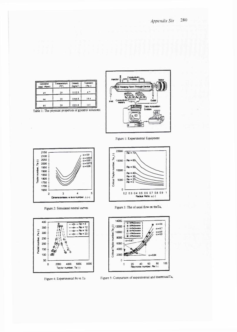
OWcerol Tcnptnniic Oomcy ViKMtyrPt.s)
43 20 1112* 47
64 20 1164* 14 4
15 20 1221 * 113
Tabic 1; The physical propcrocs of glycerol solunœ s
Appendix Six 280
Wet
Figure I : Experimental Equipment
21502100205020001950190018501800175017001650
nw w enunter, >.(-)
20000
15000
F 10000
■5 5000
02 0.3 0.4 0.5 0.6 0.7 0.8 0.9 1 Rkéu» Rat». a H
Figure 2; Simulated neutral curves Figure 3 : The of axial flow on tbeTa,
400 — RB * 8— Ô — Ra *12— 6 — Rb *18— — Rb * 23
350
300
250
200
150
100
2000 4000 6000 8000Taylor number. Ta (-)
14000
10000
5 6000
Ï 4000
5 2000
0
] o ASk&wmoi p a»0£^ tm otfanto :64«Ghen4 / Ê (%m0.7• S4«Qnnm / a«0.8□ 49ftO»t«anM a*09m 4MOMmo<
1 a « O j 6 7 ___ ,
i
0 20 40 60 80 100Reynold* nirber. Re (-)
Figure 4: Experimental Pe vs Ta Figure 5; Comparison of experimental and theoreitcalTae
Appendix Six 281
Papers SubmittedSamson S. S. Yim, M. Y. A. Lo, N. Titchener-Hooker and P. Ayazi Shamlou, 1996. Factors affecting flow instability of Newtonian liquids in Couette-Poiseuille flow. Full paper submitted for publication to Chemical Engineering Science
Factors affecting flow instability of Newtonian liquids in Couette-Poiseuille flow
S. S. S. Yim, M. V. A. Lo, N. Titchener-Hooker and P. A\3zi Shamlou^
Department of Chemical and Biochemical Engineering, University College London,
Torrington Place, London WCIE 7JE U. K.
ABSTRACT
Numerical simulations are presented showing the effects o f operating and geometrical
parameters on the transition of laminar to Taylor vortex flow for induced rotational-axial
flow in the gap of a pair of rotating cylinders. These simulations indicate that annular
rotational flow becomes more stable in the presence of a small degree of axial flow and
as gtq> width increases. The effect of rotational speed on the breakdown of laminar flow
is more conplex and for given radius ratio and axial flow rate depends on both the speed
ratio and the direction of the rotation of the cylinders, counter-rotating flow generally
producing a more stable flow than co-rotating.
Limited experimental data are provided on the residence time distribution for flow of
Newtonian liquids through the gap of two rotating cylinders. The data include results
from experiments in which flow transition occured from latninar to Taylor vortex flow.
The findings from these experiments are successfully analyzed and assessed using the
simulations studies.
* The author to whom correspondence should be addressed
Appendix Six 282
INTRODUCTION
The laminar flow field formed in the gap of two rotating coaxial cylinders has been
exploited fully by rheologists for a long time in the study of flow behaviour of Newtonian
and non-Newtonian liquids (Fredrickson, 1964; Astarita and MamiccL, 1974 and Harris,
1977). What is less known is that the induced rotational flow generated by a pair of
coaxial cylinders, especially with a small superimposed axial flow, can be used to
manipulate the residence time distribution (RTD) of various species in the g ^ in order to
promote radial mixing with negligible axial dispersion (Kataoka et al., 1975), conditions
that are considered prerequisite for good mass and heat transfer and (bio)chemical
reactions in many process engineering operations. In these unit operations, the
dependence of the RTD of the different species on the fluid flow field occurring in the
annulus is of great experimental and theoretical interests and has been the subject of
numerous studies in the past (Becker and Kaye. 1962; Coney and Simmer, 1979;
Kataoka and Takigawa, 1981; Moore and Cooney, 1995).
G. I. Taylor (1923) provided the first experimental and theoretical evidence on the
breakdown of Couette flow with increasing speed of rotation of the cylinders. With
superimposed axial flow (Couette-Poiseuille flow), the breakdown of laminar flow is a
strong function of the dimensionless axial Reynolds number. Re [ = j , the
rotational Tavlor number. Ta I = - ] . the relative speed and theI v* ;
direction of rotation of the cylinders as well as the dimensionless radius ratio, a
Appendix Six 283
The interdependence of these parameters and their combined effect on the onset of flow
instability is worthy of further investigation and is the subject of the present study. From
a process engineering point of view it is the changes in the flow structure resulting from
the breakdown of laminar flow that afreet the residence time distribution of species in the
gap and are thus thought to be responsible for the observed in^rovements in transport
and reaction processes occurring in annular rotational flow fields (Astill, 1964; Kaye and
Elgar, 1975; Cohen and Marom, 1983: Meyashita and Senna, 1993).
THEORY
The Navier-Stokes and the continuity equations governing the stability of rotational flow
o f an incompressible Newtonian liquid in the gtqs of two coaxial cylinders have so fru
been solved only for a limited number of cases, e.g. flow in narrow and wide g^ s with
zero axial flow (Walowit et a i, 1964) and flow in narrow gap with a small superimposed
axial flow (Takeuchi and Jankowski, 1981 ). In the present study, the stability problem is
formulated for the case of viscous incompressible flow of a Newtonian liquid flowing at a
low velocity through the gap of two co-rotating and counter-rotating coaxial cylinders.
The classical approach is adopted in im posing small velocity perturbations of an
exponential form on the mean flow described by the general equations, products and
squares of the perturbations are neglected and the linearised equations are made
dimensionless and are solved numerically using the Galerkin's method (DiPrima, 1955;
DiPrima and Swiimey, 1981) in order to determine the critical Taylor number at which
lam inar flow breaks down as a function of gap width, axial flow rate and the relative
speed and direction of rotation of the two cylinders.
Appendix Six 284
Thus, for these assunptions the equations for the mean flow through the gap of two
rotating cylinders are as follows.
U (r) - 0 V(r) = r CÎ (r) = A t + B/r
where
- i f
B = — Q,Rr ]-or
( 1)
(2)
and
a - Ri/Ri and 3 = Oi/Q,.
The average axial velocity, W , can be obtained by integration of Eq. (2). Thus:
, r R , y i - ( R i / r 2)=iRzV ln(R2 /R i)
(3)
(4)
(5)
The small perturbations imposed on the mean flow are assumed to be axisymmterical and
to have the following form, in accordance with most previous works (Chandrasekhar,
1961; Chung and Astill, 1977; DiPrima and Swinney, 1981)
u'(r,z,t) = ïïe’ "*’> (6a)
v'(r.z,t) = (6b)
w'(r,z,t) = we’ ' "** (6c)
p'(r.z.t) = pe‘<^'“> (6d)
where u .v .w and p are functions of r only. The two parameters s and X in Eqs. (6a) -
(6d) characterize the flow perturbations in the axial direction. Their values determine the
growth rate of the disturbance and for a given flow rate and geometry they uniquely
Appendix Six 285
determine whether the imposed perturbations will decay or be able to grow exponentially
in time leading to the formation of secondary flow in the form of Taylor vortices.
Using the cylindrical coordinate system, introducing Eqs. (6a) - (6d) into the Navier-
Stokes and continuity equations, linearising the resulting expressions and making them
dimensionless gives
^DD * -a* + i(a - aT Re)ju = Ta M v + Dp (7)
^DD • -a^ + i(a - aT Re)jv = û (8)
♦ D - a* + i(a - aT Re)jw = iap + Re(DT)û (9)
D*û + iaw = 0 (10)
where
D = -^and D* = -^ + e (11a)dx dx
r = R o + (R :-R i)x (11b)
= , 1 ,0
0 = ——— —— a = X(R2 - R i ) (lie)
M . f ! r Æ
Ù = ------— - Û V = R o Q o V ( l l g )2 A ( R 2 - R i)‘
OoRo V . __ OoRopv . . , .p = — -------------- " 7 p ( l l h )
2 A ( R 2 - R j ) 2 A ( R 2 - R i )
Appendix Six 286
Substituting Eq. (12) into Eq. (9) to eliminate w and rearranging the resulting expression
leads to
p = (d ♦ D - a + i(a - aT - - 4 ^ - ^ û (12)
Equation ( 12) is now substituted into Eq. (7) to eliminate p . Thus
(DD * -a^ + i(a - aT Re))u = Ta M v
+ D |( D * D - a = + i ( o - a T R e ) ) ( ^ ] - ^ ^ ® û | (13)
Equations (8) and (13) together with the associated boundary conditions given by;
û = Dû = v = 0 at X = ±1/2 (14)
are solved numerically by qaplying the Galerkin's technique (DiPrima, 1955) and the
calculations are performed by using the Mathematica software (version 2.2) on a Elonex
PC 560. Details of the calculation procedure and the algorithms are given elsewhere
(Yim. 1996) and are only briefly outlined here. For a fixed flow rate (axial Reynolds
R,1 . „ r «2number) and condition given by a, , and P, | = , Eqs. (8) and (13) are
solved to yield values of Taylor numbers for a range of values of the dimensionless wave
number, a (2.5 - 4.25) and a (1.169-1.236). Typical results which will be discussed later
are shown in Fig. 2 in the form of “neutral” curves for a specific radius ratio and speed
ratio at zero axial flow. The minimum point on each neutral curve defines the critical
Taylor number. Tac for the specified conditions (Walowit et al., 1964).
Appendix Six 287
EXPERIMENTAL
The residence time distribution experiments were directed towards examining the effects
of axial flow rate, gap width and the speed of rotation on the RTD of a range of glycerol-
water solutions o f different viscosities. The experiments were performed under operating
conditions that included the point of criticality. Because of limitations of the apparatus
the outer cylinder remained stationary in the experiments and flow in the gap was
induced by varying the speed of rotation of the inner cylinder which was varied between
0.0 and 400 rpm. The volumetric flow rate was varied between 2x10 and 9x10 mmVs.
The experiments were carried out in a 1 m long horizontal coaxial cylinder device in
order to minimise end effects (Fig. 1 ). The outer shell was Abricated from Perspex to
allow visual observations of the flow structure and had an inner diamete r of 90 mm,
Photographs were not taken during the experiments, but visual observations of the flow
structure was carried out to conflrm the condition of criticality. The anmilar gap width
was varied by using two inner cylinders of diameters 0.076 and 0.06 m. The inner
cylinders were constructed from stainless steel tubes and were driven by a variable speed
electric motor with rotational speed in the range of 0 - 1500 rpm. The speed of rotation
was measured by using a shaft-mounted speed transducer (2400AB Series, EEL Ltd.,
UK).
The outer shell was equipped with two electrical conductivity probes and a single
injection point. The conductivity probes were constructed from 35 mm diameter glass
rod, having two 0.315 mm diameter platinum wire electrodes mounted 2.5 mm apart.
Appendix Six 288
The two probes were separated 400 mm apart in a horizontal line with the first probe
positioned 50 mm fi*om the injection point. When in position, the tip of the electrodes
protruded 3 mm fi-om the inside wall of the outer shell. The microinjeaor was a standard
hypodermic syringe having a stainless tube of 0.7 mm outside diameter. The injection
point was 200 mm fi*om the entrance in the same horizontal line as the conductivity
probes and the tip of the injection tube was positioned at the center of the annular gap.
The tracer solution was prepared fi'om concentrated KCl (AnalaR, BDH Limhed-Poole,
England) and the woridng liquid. Injection was carried out manually within a period of
approximately 1.0 s and the tracer concentrations were recorded simultaneously and
continuously at the two probe positions as a function of time. The data fiom both
conductivity probes were stored using a data acquisition system (Keithley Model 575
measurement control system) attached to a KDAC 500/1 data collection unit and an IBM
PC2 computer for analysis and evaluation of the various parameters including the first
and second moments o f the distributions.
Prior to injection of the tracer material, steady state flow condition was established in the
apparatus by continually pumping (H.R. Flow-Inducer, Watson-Marlow Ltd., UK) the
working liquid through the annular g ^ at a fixed volumetric flow rate until the efiQux
remained constant with time. The efifiux was obtained manually by measuring the time
required to collect a known volume of the discharge liquid. Each experiment was
replicated three times and the mean value used for parameter estimation.
Appendix Six 289
RESULTS AND DISCUSSION
Figure 2 shows typical simulated neutral curves for the case of zero axial flow, a range o f
narrow gzy (a = 0.9 - 0.99) and speed ratio, p = 0. These are the conditions used by
Taylor (1923) in his formulation of the stability problem and for which the following
expression for the critical Taylor number has been recommended (Becker and Kaye,
1962). Thus
.p m/Rrn(R2 -Ri)^i c - ^ (15 )
where
(1 6 )2P (R :-R ,)'R ,
where
P = 0.0571 1 -0.0571 + 0.00056^1 -0.652 (17)
According to our plot in Fig. 2, flow becomes unstable at a Taylor number of
approximately 1700 (the minimum point on the curve, a = 0.99) which agrees well with
the predicted value (Taylor, 1923) of 1697 at a = 0.99, based on Eq. (15) to (17).
In Fig. 3, our simulations con iare well with results published by previous researchers for
the case of narrow gaps (a = 0.95). Limited experimental data reported by Snyder
( 1962) for the case of annular flow in a small gap with superimposed axial flow are also
shown in Fig. 3 and these also support the numerical simulations obtained from our
analysis of the instability problem
Appendix Six 290
Figure 4 shows the eflfea of radius ratio, a, on the critical Taylor number, Tac, with
velocity ratio, P, as a parameter. The plots are for the case of zero axial flow and
indicate that as the radius ratio decreases the critical Taylor number increases, that is, for
otherwise similar conditions, the flow becomes more stable as gap width increases.
According to the simulations shown in Fig. 4 the extent o f the increases in Tac depends
critically on the velocity ratio, p. The values o f P used in the calculations procedure are
given in Fig. 4; the negative values correspond to simulation o f flow of counter-rotating
and the positive values represent the simulation o f flow of co-rotating cylinders. It is
observed from these plots that for given radius ratio, a. the flow in the gap of a pair of
counter-rotating cylinders is significantly more stable con^ared with the case of co-
rotating cylinders.
Figure 5 shows the variation of the critical Taylor number as a function of the axial
Reynolds number. From these plots it can be seen that for fixed a and p as the flow rate
through the gap increases the critical Taylor number increases indicating that by
introducing a small degree of axial flow, the induced rotational flow becomes more
stable.
The predictions shown in Fig. 5 are confirmed by the experimental RTD data obtained
from the coaxial cylinder apparatus as discussed below. It should be noted however that
all the RTD data reported in this work are limited by the condition of zero speed ratio
since - 0.
Appendix Six 291
Typical RTD curves for the two probes are shown in Fig. 6 for four rotational speeds of
the inner cylinder in the range o f 60 to 260 rpm and axial flow velocity of 26.5 mm/s
corresponding to an axial Reynolds number. Re = 15 and Taylor numbers, Ta = 3074,
16738, 41332 and 57728 respectively. The RTD data for flow in the gap of a coaxial
cylinder apparatus has been described adequately in the past by an axial dispersion model
characterized by the dimensionless axial Peclet number, Pe^= . For the present
data the axial Peclet numbers were obtained for each experiment ly using the definition
of the variance of the distributions given by (Levenspiel 1972)
A oe^=-^ (18)
Ace represents the variance difference of the tracer RTD curves at any two points along
the annular gap. In the present study Aae' was evaluated for the g ^ between the two
probes using the response curves obtained fix)m them, as shown in Fig. 6. The value of
Aoe was substituted into Eq. (18) in order to obtain the Pe number fbr the prevailing
flow.
The effect of rotational speed on the Pe number, obtained fi-om the induise response
curves at the two conductivity probe positions is shown in Fig. 7 for four axial flow rates
expressed in term of the axial Reynolds number. The plots in Fig. 7 show that as the
rotational speed of the inner shaft increases, the Pe number increases fi-om an initial value
of about 100 to a maximum value of ^proximately 380 beyond which any further
increase in rotational speed causes a decrease in the Pe number. The minimum and
m aximum values of the Pe number were found to be functions of the flow rate through
the gap. In the present study the lowest value of Pe was found to be about 100
Appendix Six 292
corresponding to an axial flow velocity of 14 mm/s (Re = 8) and the highest value of Pe
was 380 corresponding to an axial flow velocity o f 47 mm/s (Re = 27) as shown in Fig.
7.
The variations in Pe number with increasing Ta number depicted in Fig. 7 suggests that
significant deviation fi-om plug flow conditions can occur during flow. Pudjiono et al.
(1992) and Pudjiono and Tavare (1993) in their recent publications suggested that the
maximum Pe number correspond to the conditions at which the Taylor vortices are fully
developed. In Fig. 8 we have plotted the critical Taylor number as a function of the axial
Reynolds number for the e?q)enmental conditions used in the present investigation. The
difierent symbols shown in Fig. 8 represent the experimental critical Taylor numbers
obtained fi-om the Peclet number - Taylor number plots such as those shown in Fig. 7
while the solid curves are the simulations. The agreement between theory and
experiments is considered satisâctory.
CONCLUSIONS
Theoretical equations are developed and are numerically solved for the onset of flow
instability in combined Couette and Poiseuille flow. The formulation is applicable to flow
of Newtonian liquids through wide gaps formed between two co-rotating and counter-
rotating cylinders. The numerical simulations are presented in terms of the critical Taylor
number as a function of three dimensionless groups afiecting it, i.e. the axial Reynolds
number, the dimensionless radius ratio and the relative speed of rotation of the two
cylinders. The results indicate that for otherwise similar conditions, rotational flow in the
Appendix Six 293
gap becomes more stable as the axial Reynolds increases and as the dimensionless radius
ratio decreases. The efifect of speed of rotation is more complex and depends on the
direction as well as the absolute values of the speed of the two cylinders.
Limited residence time distribution data were obtained fbr the axial dispersion of a tracer
fluid in the gap of a coaxial cylinder apparatus operating close to the Taylor-Couette-
Poiseuille regime. The analysis of RTD data showed a systematic variation in the
prevailing axial Peclet number. This variation was explained adequately in terms of the
changing flow structure in the gap as flow approached the point o f criticality. The
experimental observations based on the RTD data and the associated numerical
simulations presented have inqx)rtant implications for the design and operation of
equipment in which Taylor-Couette-Poiseuille flow is used to enhance transport and
reaction processes.
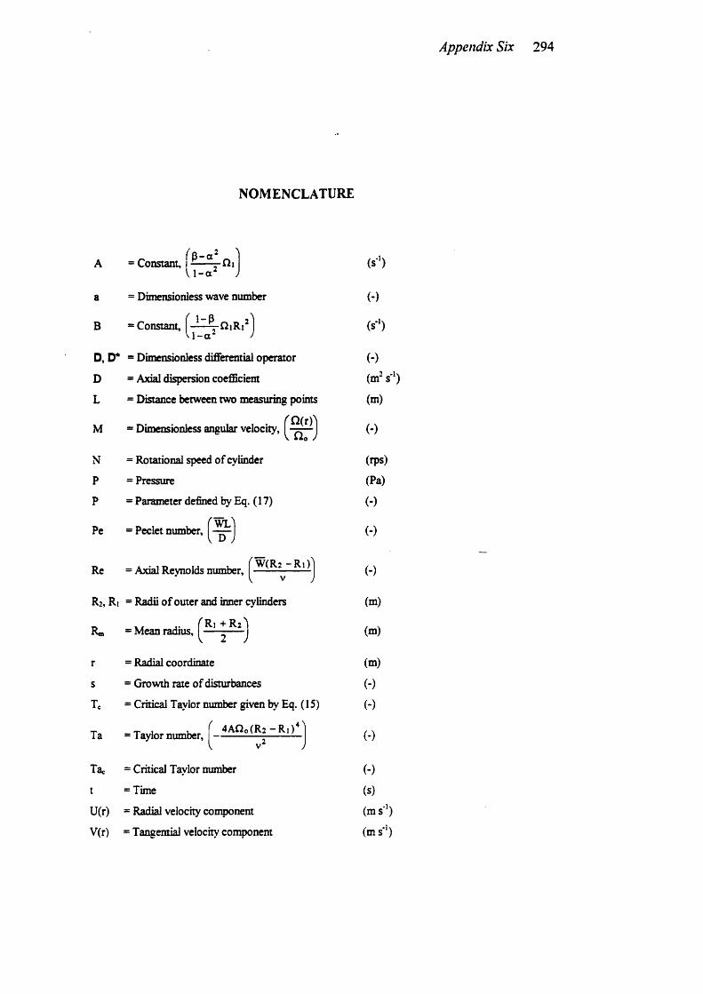
Appendix Six 294
NOMENCLATURE
A_ B -a _= Constant, ------;-Gi
l i - o / ;(s*‘)
a = Dimensionless wave number (-)
B = Constant, |~ - y f i iR i^ j (s')
D,D* = Dimensionless differential operator (-)
D = Axial dispersion coefBcient (m's*')
L = Distance between two measuring points (m)
M = Dimensionless angular velocity, (-)
N = Rotational speed of cylinder (rps)
P = Pressure (Pa)
? = Parameter defined by Eq. (17) (-)
Pe = Peclet number, (-)
Re = Axial Reynolds number, I —— I (-)
Rj, Ri = Radii of outer and inner cylinders (m)
R= = Mean radius, (m)
r = Radial coordinate (m)
s = Growth rate of disturbances (-)
Te = Critical Taylor number given by Eq. ( 15) (-)
Ta = Taylor number, (-)
Tac = Critical Taylor number (-)
t = Time (s)
U(r) = Radial velocity component (m s')
V(r) = Tangential velocity component (ms"')
w = Axial flow velocity (m s ')
W(r) = Axial velocity conyonent (m s’’)
X = Transformed dimensionless radial coordinate (-)
z = Axial coordinate (m)
Greeks Symbols
Appendix Six 295
= Radius ratio'& )
XnV
aAoe
= Angular speed ratio,
= Weighting function
= Dimensionless constant,
= Wave number
= Viscosity of the working liquid
= Kinematics viscosity of the working liquid
= Dimensionless growth rate
= Dimensionless variance difference
Q2, = Angular velocities of outer and inner cylinders
Qo = Average angular velocity
O (r) = Angular velocity
Û) = Angular velocity given by Eq. ( 16)
4 = Dimensionless variable
(-)
(-)
(')
(-)
(m*‘)
(kg m*' s"’)
(kg m’’ s ')
(■) —
(-)
(rad-')
(rad-')
(rad*')
(rad-')
(-)
Superscripts and Subscripts
= Average value
= Perturbed quantity
= Eigenfunction given by Eqs. (4) - (7)
= Dimensionless eigenfunction
= Critical value
Appendix Six 296
REFERENCES
1. Astrarita, G. and Mamicci, G., 1974, Principles o f non-Newtonian fluid
mechanisms, McGraw-Hill, London.
2. Astill, K. N., 1964, Studies of the developing flow between concentric cylinders
with the inner cylinder rotating, J. Heat Transfer Trans. ASME., C86, 383-392.
3. Becker, K. M. and Kaye, J., 1962, The influence of a radial tenqxrature gradient
on the instability of fluid flow in an annulus with an inner rotating cylinder. J.
Heat Tranter Trans. ASME, C84,383-392.
4. Chandrasekhar, S., 1960, The hydrohynamic stability o f viscid flow between
coaxial cylinders, Proc. Nat. Acad. Sci., 46, 141.
5. Chandrasekhar, S., 1961, Hydrodnamic and Hydromagnetic Stability, Oxford:
Clarendon Press, London.
6. Chung, K. C. and Astill, K. N., 1977, Hydrodynamic instability o f viscous flow
between rotating coaxial cylinders with fully developed axial flow, J. Fluid
Meek, 81(4), 641-655.
7. Cohen, S. and Marom, D. M., 1983, Experimental and theoretical study of a
rotating annular flow reactor, Chem. Engng J., 27, 87-97.
8. Coney, J. E. R. and Simmers, D. A., 1979, A study of fully-developed, laminar,
axial flow and Taylor vortex flow by means of shear stress measurements, J. Meek Engng Sci., 19-24.
9. DiPrima, R. C., 1955, Application of the Galerkin method to problems in
hydrodynamic stability. Quart. Applied Mathematics, 13, 55-62.
10. DiPrima, R. C., and Swinney, H. L., 1981. Stabilities and Transition in Flow
between Concentric Rotating Cylinders, In Hydroefynamic Instabilties and the
Transition to Turbulence (ed. H. L. Swinney and J. P. Gollub), Chap. VI,
Springer-Verlag, Berlm.
11. Elliott, L., 1973, Stability of a viscous fluid between rotating cylinders with axial
flow and pressure gradient round the cylinders, Phys. Fluids, 16(5), 577-580.
12. Fredrickson, A. G., 1964, Principles and applications o f rheology, Prentic-Hall,
London.
13. Harris, J., 1977, Rheology and non-Newtonian flow, L ongm an, London.
Appendix Six 297
14. Kataoka, K, and Takigawa. T.. 1981. Intermixing over cell boundary between
Taylor vortices, ,/4/CA£ 7., 27, 504-508.
15. Kataoka, K., Doi, H., Hongo, T. and Futagawa, M , 1975, Ideal plug-flow
properties o f Taylor vortex flow, J. Chem. Engng Japan, 8,472-476.
16. Kaye, J. and Elgar, E. C., 1958, Modes of adiabatic and diabaiic fluid flow in an
annulus with an inner rotating cylinder, Trans. ASME, 80, 753-765.
17. Levenspiel, O., 1972, Chemical Reaction Engineering, 2nd ed.. Chuter IX,
Wiley, New York.
18. Miyashita, T. and Senna, M., 1993, Development of Taylor vortices in a
concentrated suspension conqmsing monodispersed microspheres, J. Colloid
Interface Sci., 155,290-296.
19. Moore, C. M. V. and Cooney C. L., 1995, Axial dispersion in Taylor-Couette
flow, AIChEJ., 42(3), 723-727.
20. Pudjiono, P.I., Tavare, N.S., Garside, J. and Nigam, K.D.P., 1992, Residence
time distribution from a continuous Couette flow device, Chem. Engng J., 48,
101- 110.
21. Pudjiono, P.I. and Tavare, N.S., 1993, Residence time distribution analysis from a
continuous Couette flow device around ciritical Taylor number. Can. J. Chem.
Engng, 71(4), 312-318.
22. Snyder, H. A., 1962, Stability of spiral flow at low Reynolds number, Proc. Roy.
Soc., A265, 198-213.
23. Takeuchi D. I. and Jankowski, D. P., 1981, A numerical and experimental
investigation of the stability of spiral Poiseuille flow, J. Fluid Mech., 102. 101-
126.
24. Taylor, GJ., 1923, Stability of viscous liquid contained between two rotating
cylinders. Phil. Trans. Roy. Soc. (London), A233,289-343.
25. Walowh, J., Tsao, A. and DiPrima, R. C., 1964, Stability of flow between
arbitrarily spaced concentric cylinderical surfrces including effect of a radial
tenqjerature gradient, J. Applied Mechanics Tran. ASME, 31, 585-593.
26. Yim, S. S. S., 1996, Residence time distribution (RTD) studies in a rotary flow
through device, PhD Thesis, Unverisity College London, (in preparation).
Appendix Six 298
CAPTIONS
Figure 1 Typical simulated neutral curves obtained from
the solution of Eq. (8) and Eq. (13)
Figure 2 Experimental equipment
Figure 3 Conqaarison of numerical simulations and experimental data
for rotational-axial flow in the small gap of a pair of rotating cylinders
Figure 4 Simulated critical Taylor number vs Radius Ratio
(at different speed ratio)
Figure 5 The effect of axial flow on the critical Taylor number
as a function of radius ratio
Figure 6 The effect of rotational speed on residence time distribution
Figure 7 Experimental Peclet number vs Taylor number at different
axial Reynolds numbers Radius Ratio = 0.84
Figure 8 Comparison of experimental and theoretical critical Taylor numbers
as function of the axial Reynolds number
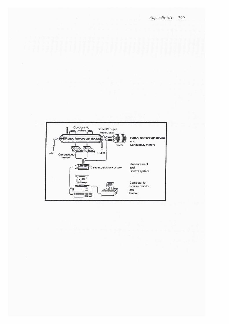
Appendix Six 299
Speed/T orque transducer
ÎInlet
* uonoucuvny
Rotary flowHhrough device
Conductivitymeters
Outlet
Rotary AowMhrough device ^ and
motor ConductMy meters
Data acquisition system
n = = ^ É .
MeasurementandControl system
Computer for Screen monitor and Printer
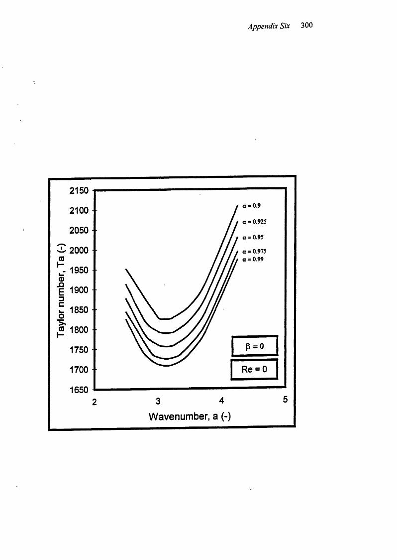
Appendix Six 300
2150 1a = 0.92100a = 0.925
2050a = 0.95
2000 a = 0.975 a = 0.99
^ 1950 0)E 1900
i. 1850 - *JO
1800
p = 01750
Re = 01700
1650
Wavenumber, a (-)
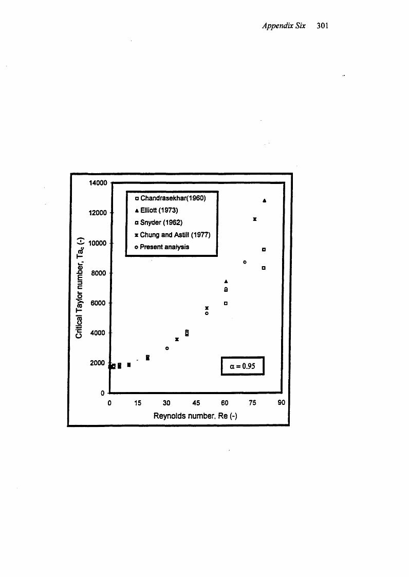
Appendix Six 301
14000
12000
^ 10000eo
o>• | 8000
o! • 6000
sg 4000
2000
o Chandrasekhar(1960)
A Elliott (1973)
Q Snyder (1962)
X Chung and Astlll (1977)
o Present analysis
a i ■ a = 0.95
15 30 45 60
Reynolds number. Re (-)
75 90
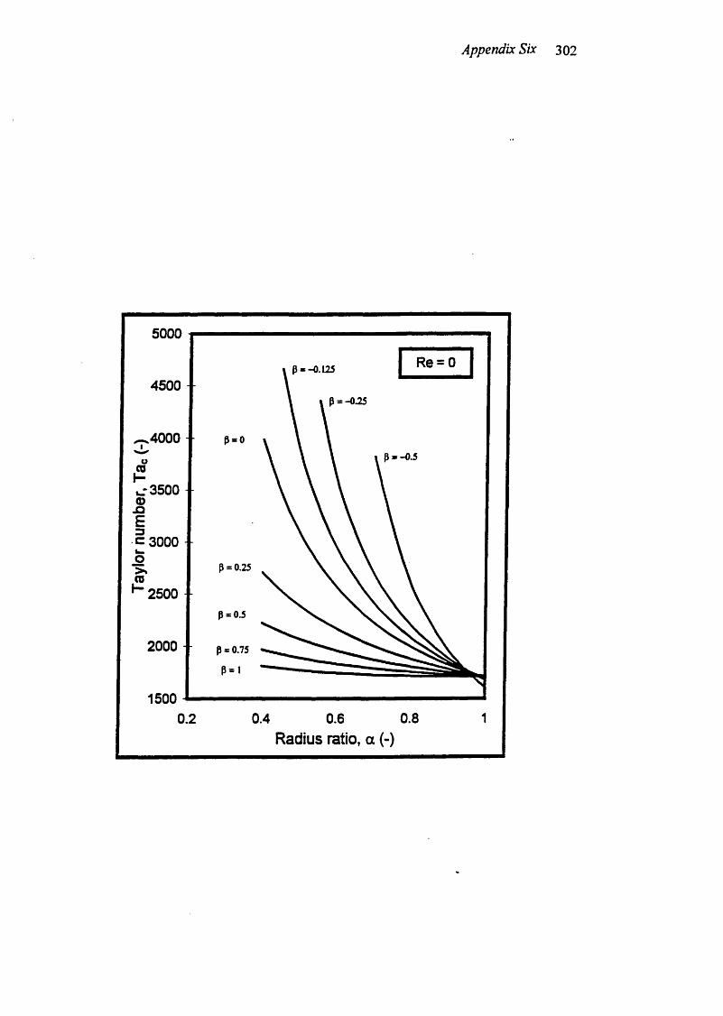
Appendix Six 302
5000
Re = 04500
4000 p = o
.-3500 - ■
c 3000 -
= 0.25
2500 -
2000 ■ - 0.75
1500 -I0.80.4 0.6
Radius ratio, a (-)0.2
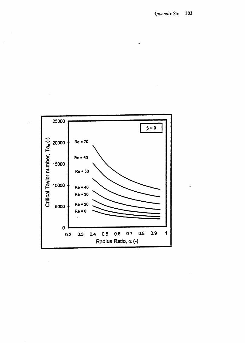
Appendix Six 303
25000P = 0
20000 - - Re s 70
R e » 6 0
E 15000 -R e * 5 0
P 10000 - R3.40
R R e * 3 0
O 5000 ■ * 20R e * 0
Radius Ratio, a (-)
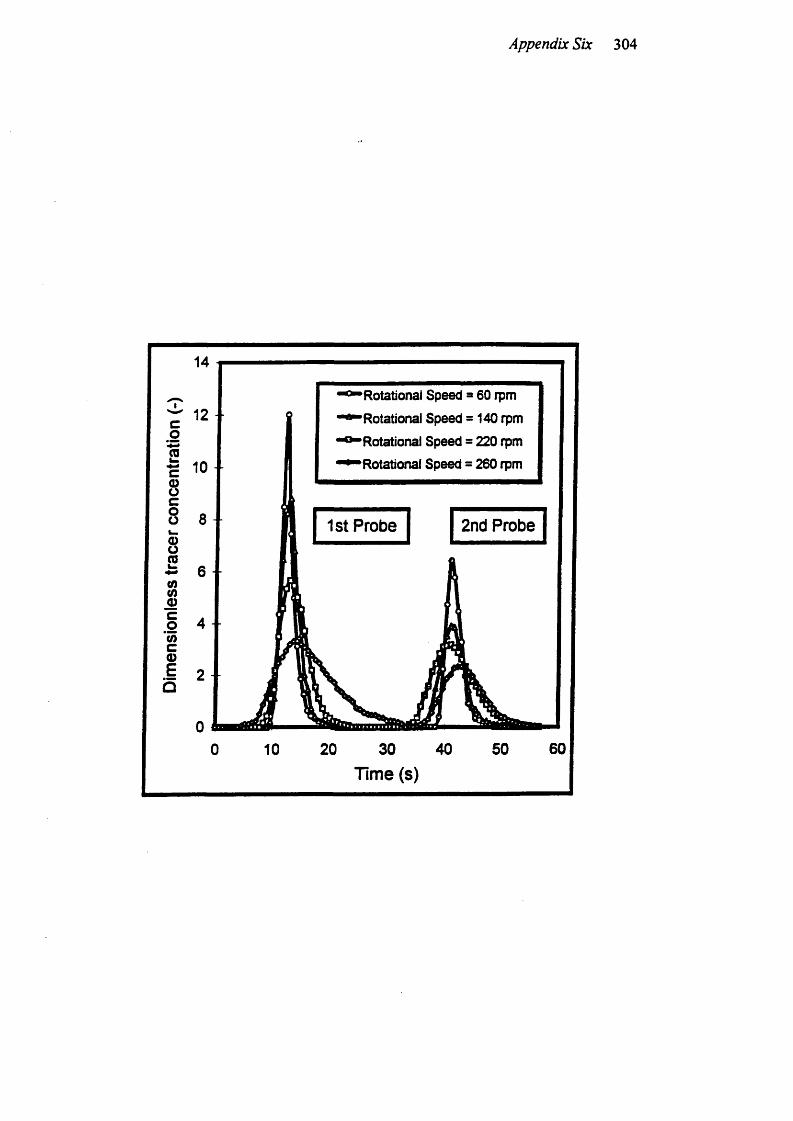
Appendix Six 304
14
2nd Probe1st Probe
Rotational Speed = 60 rpm
"Rotational Speed = 140 rpm
Rotational Speed = 220 rpm
Rotational Speed = 260 rpm
10 20 30 40Time (s)
50 60
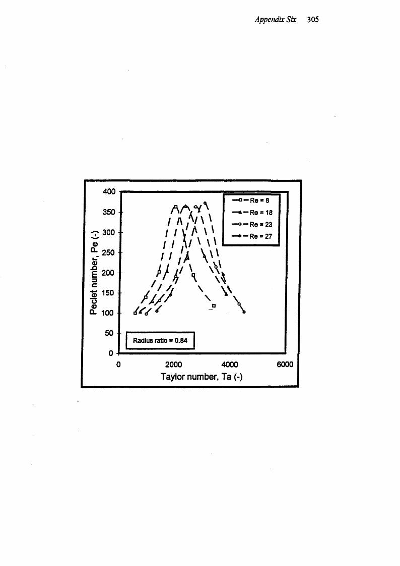
Appendix Six 305
400— Re * 8
350
250
E 200
150
(L 100 / / / ^
50Radius ratio « 0.84
60002000Taylor number, Ta (-)
4000
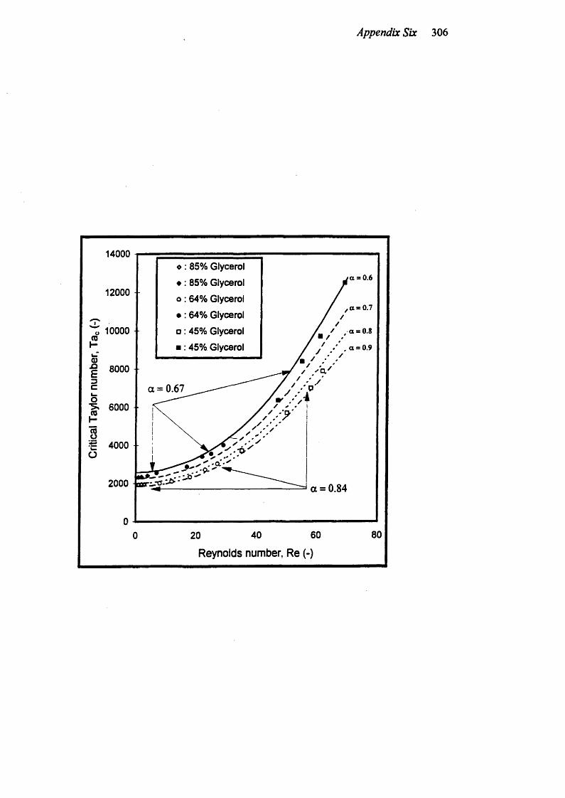
Appendix Six 306
14000o : 85% Glycerol
♦ : 85% Glycerol
o : 64% Glycerol
• : 64% Glycerol
□ : 45% Glycerol
■ : 45% Glycerol
a = 0 . 6
12000a = 0 . 7
10000 a = 0.8■ /
a = 0 . 9
8000
a = 0.67
^ 6000
4000 ■
2000 a = 0.84
Reynolds number, Re (-)