thesis.pdf - ucl discovery
TRANSCRIPT

Computational investigations of the speciation of Sr2+
in aqueous solution, and its interactions with thehydrated brucite (0001) surface
Eszter Makkos
A thesis submitted for the degree of
Doctor of Philosophy in Computational Chemistry
Department of Chemistry
University College London
April, 2017


I, Eszter Makkos confirm that the work presented in this thesis is my own.
Where information has been derived from other sources, I confirm that this
has been indicated in the thesis.


Abstract
The fundamental objective of this research project was to develop a computational model,
using high-level quantum chemical techniques based on density functional theory (DFT),
which is able to describe the aquo and hydroxide complexes of strontium and their inter-
actions with hydrated brucite surfaces, aiming to create a general approach which can be
subsequently modified for the investigation of other radioactive ions/surfaces. The first two
chapters of this PhD thesis are a general introduction on the project’s industrial relevance
and on the computational methodology used. The subject of this study is strongly related to
the decommissioning of the UK’s nuclear legacy fuel storage ponds and therefore the the-
sis is organised such that, through the three main steps of the computational investigation, it
eventually leads to an industrially relevant main conclusion.
In the third chapter, the possible strontium hydroxide complexes in aqueous environment
have been investigated, in order to establish likely candidate species for the interaction of nu-
clear fission-generated strontium with the hydrated brucite surfaces in high pH spent nuclear
fuel storage ponds. A combination of the COSMO continuum solvation model and one or
two shells of explicit water molecules are employed for describing accurately the hydrolysis of
Sr2+.
The next chapter presents the periodic electrostatic embedded cluster model, developed
for the brucite (0001) surface to be employed in the study of the adsorption reactions. Using
the periodic electrostatic embedded cluster method (PEECM), implemented in the TURBO-
MOLE code, we have created a quantum chemically treated cluster in an infinite array of point
charges and validated this surface model by exploring the adsorption of Sr2+ and other s block
cations on bare and hydrated surfaces, comparing the PEECM data with those from a periodic
DFT study using the CRYSTAL code.
In the fifth chapter, the results of the previous two chapters are combined to describe
the Sr-surface interactions as realistically as possible. A theoretical reaction was created, in
which the energy of the adsorbed Sr2+ ion on a hydrated brucite surface was compared with
the energy of a solvated Sr2+ in the bulk solution, i.e. with the previously identified strontium
complexes in aqueous phase. To achieve this, the PEECM model was extended with one and
two layers of water molecules both in the quantum mechanical and point charge region, whose
geometries are based on previous molecular dynamics studies. Several possible complexes
are identified both in the presence or absence of solvated OH− groups with different Sr-surface
distances and complex conformation, and their adsorption energies were calculated in order
to evaluate the general strength of the possible ion-surface interactions.


Acknowledgement
There are numerous people to thank for all the help and encouragement which I received
during my PhD studies and in completing this thesis. First, I owe special gratitude to my
supervisor Nik Kaltsoyannis; without his kind guidance and support throughout this work would
never have been completed. He was there to keep me on track when I was about to be lost in
details and he has always been calm and supportive even when I had doubts about my results.
Similar thanks to Andy Kerridge, my second supervisor. All his help; his previous work on the
topic, his incredibly useful advice and general encouragement; both fuelled and improved this
thesis. I would like to extend my gratitude to all my fellow PhD students who were there during
my studies at UCL. I feel very fortunate to have such a good friends, all of them intelligent,
funny and helpful. Special thanks must go to the ”Eamonn’s Anti-abandonment group”: Abi,
Belle, Eamonn, Joe, and Toby; it was an honour to be in the same shoe with you guys! I would
like to mention by names two more of my friends in this paragraph, their advice and help in
work, besides their friendship, means a lot to me: thanks David and Enrico.
This work was half-funded by the National Nuclear Laboratory and National Decommis-
sioning Authority, I am very grateful for their financial and technical support. Particular mention
to my industrial supervisor, Jonathan Austin, whose guidance concerning the nuclear industry
and patient explanations of my project’s industrial relevance helped to finish this work with
results beneficial on both sides. This amount of data would never been produced without the
several computer sources accessible to me and I am grateful for all of these services. I would
like to acknowledge the use of the ARCHER UK National Supercomputing Service, the com-
puting resources from UCL via the Research Computing ”Legion” and ”Grace” clusters and
associated services and the late EPSRC UK National Service for Computational Chemistry
Software (NSCCS) at Imperial College London, and the ”Iridis” facility of the e-Infrastructure
South Consortiums Centre for Innovation. Personally, I would like to thank my previous group
at the Budapest University of Technology and Economics, for their invaluable support in my
previous studies and in the field of quantum chemical calculations which lead me to start and
complete a PhD in this field.
At last but not least, I would like to thank for every member of my family: especially my
parents, my sister Vera, my grandparents, godparents, cousins and all of my friends from
home or abroad (I cannot possibly list you on a single page, but I hope you all know who you
are!). Their unquestioning belief in my capabilities and their unconditional love helped me to
also believe that I can achieve anything that I start. Finally, I left you for last Ors, because I
cannot possibly express my gratitude towards you. Thank you for your infinite care, optimism
and willpower which were and still continue to be a great inspiration for me.

Szeretnem magyarul is megkoszonni csaladom minden tagjanak: kulonosen szuleimnek,
noveremnek Veranak, nagyszuleimnek, keresztszuleimnek, unokatestvereimnek, es minden
kedves baratomnak otthon es kulfoldon. (Egy oldal is keves lenne mindannyiotokat nevvel
felsorolni, de remelem mind tudjatok, hogy ratok gondolok!) A ti kerdes nelkuli bizalma-
tok a kepessegeimben es a feltetel nelkuli szeretetek segıtett, hogy en is elhiggyem, kepes
vagyok barmit veghez vinni amibe belekezdek. Es vegul, utoljara hagytalak teged Ors, mert
keptelenseg szavakkal kifejezni a halat amit feled erzek. Koszonom a vegtelen gondoskodasod,
az optimizmusod es akaraterod, tulajdonsagok amiket mindig is csodaltam benned es minden
nap engem is uj erovel toltenek el.


Contents
List of Figures iv
List of Tables xii
1 Introduction 1
1.1 The legacy of Magnox reactors . . . . . . . . . . . . . . . . . . . . . . . . . . . 2
1.2 Hazardous radioactive ions in the ponds . . . . . . . . . . . . . . . . . . . . . . 4
1.3 SIXEP: the pond water treatment process . . . . . . . . . . . . . . . . . . . . . 5
1.4 Computational challenges . . . . . . . . . . . . . . . . . . . . . . . . . . . . . 7
1.4.1 Studying the hydrolysis of Sr2+ in aqueous environment . . . . . . . . . 7
1.4.2 Creating a suitable surface representation of (0001) brucite surface . . . 8
1.4.3 Studying the interactions between the solvated Sr2+ and hydrated (0001)
brucite surface . . . . . . . . . . . . . . . . . . . . . . . . . . . . . . . . 9
2 Electronic Structure Theory 10
2.1 The Schrodinger equation and other approximations . . . . . . . . . . . . . . . 10
2.2 Hartee-Fock theory (HF) . . . . . . . . . . . . . . . . . . . . . . . . . . . . . . 13
2.3 Density Functional Theory (DFT) . . . . . . . . . . . . . . . . . . . . . . . . . . 15
2.3.1 Exchange-Correlation Functionals . . . . . . . . . . . . . . . . . . . . . 18
2.3.2 Dispersion correction . . . . . . . . . . . . . . . . . . . . . . . . . . . . 21
2.3.3 Resolution of identity . . . . . . . . . . . . . . . . . . . . . . . . . . . . 21
2.4 Basis Sets . . . . . . . . . . . . . . . . . . . . . . . . . . . . . . . . . . . . . . 22
2.4.1 Effective Core Potentials (ECPs) . . . . . . . . . . . . . . . . . . . . . . 24
2.4.2 Basis Set Superposition Error (BSSE) . . . . . . . . . . . . . . . . . . . 25
2.5 Solvent Models . . . . . . . . . . . . . . . . . . . . . . . . . . . . . . . . . . . 25
2.5.1 Continuum Solvent Models (CSM) . . . . . . . . . . . . . . . . . . . . . 26
2.6 Periodic Electronic Structure Methods . . . . . . . . . . . . . . . . . . . . . . . 29
2.6.1 Periodic Density Functional Theory . . . . . . . . . . . . . . . . . . . . . 30
2.6.2 Periodic Electrostatic Embedded Cluster Method (PEECM) . . . . . . . . 32
2.7 Calculations In Practice . . . . . . . . . . . . . . . . . . . . . . . . . . . . . . . 34
2.7.1 Geometry Optimisation . . . . . . . . . . . . . . . . . . . . . . . . . . . 35
2.7.2 Frequency Calculation . . . . . . . . . . . . . . . . . . . . . . . . . . . 36
2.7.3 Electronic Structure Analysis . . . . . . . . . . . . . . . . . . . . . . . . 37
2.7.3.1 Quantum Theory of Atoms in Molecules (QTAIM) . . . . . . . . 37
2.7.3.2 Natural Population Analysis (NPA) . . . . . . . . . . . . . . . . 39
i

ii CONTENTS
2.7.3.3 Mapping the Electron Density Difference . . . . . . . . . . . . 40
2.7.4 Codes . . . . . . . . . . . . . . . . . . . . . . . . . . . . . . . . . . . . 41
2.7.4.1 TURBOMOLE . . . . . . . . . . . . . . . . . . . . . . . . . . . 41
2.7.4.2 CRYSTAL . . . . . . . . . . . . . . . . . . . . . . . . . . . . . 42
2.7.4.3 AIMALL . . . . . . . . . . . . . . . . . . . . . . . . . . . . . . 43
2.7.4.4 Multiwfn . . . . . . . . . . . . . . . . . . . . . . . . . . . . . . 43
3 Simulation of hydrated Sr2+ hydroxide complexes: the importance of second
shell effects 44
3.1 Introduction . . . . . . . . . . . . . . . . . . . . . . . . . . . . . . . . . . . . . 44
3.2 Literature review: Previous solvation studies on Sr2+ . . . . . . . . . . . . . . . 44
3.2.1 Sr2+ hydrates in gas phase . . . . . . . . . . . . . . . . . . . . . . . . . 44
3.2.2 Sr2+ hydrates in aqueous phase . . . . . . . . . . . . . . . . . . . . . . 46
3.2.3 The order and dynamics of hydration shells . . . . . . . . . . . . . . . . 48
3.2.4 Sr2+ hydroxides . . . . . . . . . . . . . . . . . . . . . . . . . . . . . . . 49
3.3 Computational details . . . . . . . . . . . . . . . . . . . . . . . . . . . . . . . . 51
3.3.1 Solvation effects . . . . . . . . . . . . . . . . . . . . . . . . . . . . . . . 52
3.3.2 Thermodynamic contributions . . . . . . . . . . . . . . . . . . . . . . . 52
3.4 Results . . . . . . . . . . . . . . . . . . . . . . . . . . . . . . . . . . . . . . . . 53
3.4.1 Sr2+ hydroxide complexes with a first solvation shell . . . . . . . . . . . 53
3.4.2 Sr2+ hydroxide complexes with a first and second solvation shells . . . . 55
3.4.2.1 Proton transfer between solvation shells . . . . . . . . . . . . . 63
3.4.3 The relative stability of Sr2+ hydroxide complexes in the presence of two
explicit solvation shells . . . . . . . . . . . . . . . . . . . . . . . . . . . 66
3.5 Conclusions . . . . . . . . . . . . . . . . . . . . . . . . . . . . . . . . . . . . . 69
4 Modelling the (0001) brucite surface with the periodic electrostatic embedded
cluster method 71
4.1 Introduction . . . . . . . . . . . . . . . . . . . . . . . . . . . . . . . . . . . . . 71
4.2 Literature review . . . . . . . . . . . . . . . . . . . . . . . . . . . . . . . . . . . 71
4.2.1 The structure of the mineral brucite . . . . . . . . . . . . . . . . . . . . 71
4.2.2 Electronic structure and bond analysis . . . . . . . . . . . . . . . . . . . 73
4.2.3 Interlayer forces in brucite . . . . . . . . . . . . . . . . . . . . . . . . . . 75
4.2.4 Surface structure and cleavage . . . . . . . . . . . . . . . . . . . . . . . 76
4.3 Modelling ionic adsorption on surfaces . . . . . . . . . . . . . . . . . . . . . . . 78
4.4 Computational details . . . . . . . . . . . . . . . . . . . . . . . . . . . . . . . . 80
4.4.1 PEECM models . . . . . . . . . . . . . . . . . . . . . . . . . . . . . . . 80
4.4.2 Periodic DFT models . . . . . . . . . . . . . . . . . . . . . . . . . . . . 88

CONTENTS iii
4.5 Results . . . . . . . . . . . . . . . . . . . . . . . . . . . . . . . . . . . . . . . . 91
4.5.1 Single ion adsorption of Sr2+ and other s block elements on brucite . . . 91
4.5.2 Adsorption of Sr2+ hydrates . . . . . . . . . . . . . . . . . . . . . . . . 99
4.5.3 Substitution of Ca2+ and Sr2+ into brucite . . . . . . . . . . . . . . . . . 103
4.5.4 Adsorption of Sr[(OH)2(H2O)4] on brucite . . . . . . . . . . . . . . . . . 106
4.6 Conclusions . . . . . . . . . . . . . . . . . . . . . . . . . . . . . . . . . . . . . 113
5 Studying the interaction between solvated Sr2+ and the hydrated (0001) brucite
surface 115
5.1 Introduction . . . . . . . . . . . . . . . . . . . . . . . . . . . . . . . . . . . . . 115
5.2 Literature review . . . . . . . . . . . . . . . . . . . . . . . . . . . . . . . . . . . 115
5.2.1 Sorption processes at water/solid interfaces . . . . . . . . . . . . . . . . 115
5.2.2 Hydration of MgO and Mg(OH)2 surfaces . . . . . . . . . . . . . . . . . 117
5.2.3 Adsorption studies on brucite . . . . . . . . . . . . . . . . . . . . . . . . 121
5.3 Computational details . . . . . . . . . . . . . . . . . . . . . . . . . . . . . . . . 123
5.3.1 Introducing water layers above the brucite surface . . . . . . . . . . . . 124
5.4 Results . . . . . . . . . . . . . . . . . . . . . . . . . . . . . . . . . . . . . . . . 127
5.4.1 Adsorption of Sr2+ on a hydrated brucite surface . . . . . . . . . . . . . 128
5.4.2 Adsorption of Sr2+ hydroxides on a hydrated brucite surface . . . . . . . 134
5.4.3 The relative stability of Sr2+ complexes on a hydrated brucite surface . . 138
5.4.3.1 Interaction energies in different coordination regimes . . . . . . 138
5.4.3.2 The effect of solvated OH- ions . . . . . . . . . . . . . . . . . . 143
5.5 Conclusions . . . . . . . . . . . . . . . . . . . . . . . . . . . . . . . . . . . . . 147
6 Conclusions 149
6.1 Computational achievements . . . . . . . . . . . . . . . . . . . . . . . . . . . . 149
6.1.1 Studying the hydrolysis of Sr2+ in aqueous environment . . . . . . . . . 149
6.1.2 Creating a suitable surface representation of (0001) brucite surface . . . 150
6.1.3 Studying the interactions between the solvated Sr2+ and hydrated (0001)
brucite surface . . . . . . . . . . . . . . . . . . . . . . . . . . . . . . . . 151
6.1.4 Future Works . . . . . . . . . . . . . . . . . . . . . . . . . . . . . . . . 151
6.2 Industrial relevance . . . . . . . . . . . . . . . . . . . . . . . . . . . . . . . . . 152
Appendices 179
A Periodic DFT models 180

List of Figures
1.1 Example of a nuclear legacy pond and a Magnox-type fuel element . . . . . . . 2
1.2 ESEM images of (a) a Magnox model sample, (b) corrosion products of Mag-
nox: brucite and other Mg based phases (c) in-situ formed uranium-oxide par-
ticles[11] . . . . . . . . . . . . . . . . . . . . . . . . . . . . . . . . . . . . . . . 3
1.3 Schematic diagram of fission product yield for thermal neutron fission of 235U
and 239Pu . . . . . . . . . . . . . . . . . . . . . . . . . . . . . . . . . . . . . . 4
1.4 The process diagramm of SIXEP[2] . . . . . . . . . . . . . . . . . . . . . . . . 6
2.1 Schematic comparison of the radial function in Slater and Gaussian Type Orbitals 23
2.2 Different definitions of the cavity surface[102] . . . . . . . . . . . . . . . . . . . 27
2.3 Schematic representation of the different regions in PEECM calculations in the
x direction . . . . . . . . . . . . . . . . . . . . . . . . . . . . . . . . . . . . . . 33
3.1 The most stable Sr(H2O)2+24 according to Boda et al. contains 8 water molecules
directly coordinated to the Sr2+ ion. The left structure is optimised in gas phase,
while the right one with the COSMO implicit solvation model.[150] . . . . . . . . 45
3.2 Mehandzhiyski et al. studied the solvated complexes of alkaline earth metal
ions with different ionic radii by BOMD simulations[151]: (a) Successive water
binding energies (∆E) for different alkaline earth metal cations as a function of
the coordination number (b)Radial distribution functions between the metal ions
and the oxygen of the water molecules . . . . . . . . . . . . . . . . . . . . . . . 46
3.3 The plots, delivered by Hofer et al.[170], show the changes in the Sr-O dis-
tances during the simulation period (a); and the coordination numbers as a
function of time in the second (b) and first solvation shell (c) . . . . . . . . . . . 49
3.4 Optimised structures of Sr(H2O)5(OH)+ and Sr(H2O)7(OH)+complexes in gas
phase by Felmy[142]. The OH− is coloured on the pictures. . . . . . . . . . . . 51
3.5 Optimised structure of the W24 water cluster reported by Ludwig and Wein-
hold[190] . . . . . . . . . . . . . . . . . . . . . . . . . . . . . . . . . . . . . . . 56
3.6 Optimised structures of two Sr2+ hydrates with a first solvation shell (ball and
stick) surrounded by an explicit second solvation shell (represented as tubes),
along with their relative SCF and free energies (∆ESCF /∆G). (Sr2+=magenta,
O=red in water molecules, H=white). Energies are given in kJ/mol. . . . . . . . 56
iv

LIST OF FIGURES v
3.7 Relative free energies (∆G) of structures containing 22 water molecules and 2
hydroxide ions calculated compared to the most stable structure optimised with
COSMO (W24 OH c). Complexes optimised with and without solvent model
are represented with white and red bars respectively. . . . . . . . . . . . . . . 59
3.8 Relative SCF energies (∆E) of structures containing 22 water molecules and 2
hydroxide ions calculated compared to the most stable structure optimised with
gas phase (W24 OH2 d). Complexes optimised without solvent model are rep-
resented with red bars, while COSMO single point energies with black diagonal
stripes. . . . . . . . . . . . . . . . . . . . . . . . . . . . . . . . . . . . . . . . 60
3.9 Optimised structures of two Sr2+ hydroxides, surrounded with 24 water molecules.
The non-directly coordinated ligands are represented as tubes. The [Sr:5/17:1/1]
(W24 OH2 c in Table 3.5), which are based on a pre-optimised water cluster,
is 14.2 kJ/mol more stable than the ’built-up’ structure (C1m 22d in Table 3.5),
[Sr:6/16:1/1], and contains more hydrogen-bonds. (relative SCF and free en-
ergies are shown as (∆ESCF /∆G); Sr2+=magenta, O=red in water molecules,
O=blue in OH− ions, H=white). Energies are given in kJ/mol. . . . . . . . . . . 60
3.10 Ball and stick figure of the optimised geometry of the [Sr:5/18:1/0]+ monohy-
droxide with two complete solvation shell, based on the W24 water cluster,
viewed from the side (a) and the top (b). The second shell waters are repre-
sented by tubes. (Sr2+=magenta, O=red in water molecules, O=blue in OH−
ions, H=white). . . . . . . . . . . . . . . . . . . . . . . . . . . . . . . . . . . . . 62
3.11 Free energy profile (∆G) of proton transfer between the most stable dihydrox-
ide ([Sr:4/18:2/0]) and monohydroxide ([Sr:5/17:1/1]) complexes with 22 water
molecules, from the second column of Table 3.8. TS = transition state. . . . . . 65
3.12 Gibbs free energies (∆G, kJ/mol) (a) for Eq. (3.2), and (b) for Eq. (3.3) for
systems with 1 to 4 hydroxide ions. . . . . . . . . . . . . . . . . . . . . . . . . . 68
4.1 The layered structure of brucite showing the typical unit cell, beside the side
and top view of the octahedral Mg coordination.[202] . . . . . . . . . . . . . . . 72
4.2 Total and projected DOS of the bulk and slab brucite obtained by D’Arco et
al.[200] . . . . . . . . . . . . . . . . . . . . . . . . . . . . . . . . . . . . . . . . 74
4.3 Representation of the valence ELF for the (110) plane of brucite, containing one
(left) and two (right) units of Mg-OH. ELF values increase from blue to red.[217] 74

vi LIST OF FIGURES
4.4 Optimised structures of the possible cleavages of the brucite surface: (a) side
view of the (0001) structure, (b) of the (1100) surface and (c) of the (1120)
cleavage. The dotted lines indicate the atomic planes in the surface, while the
numbers are interatomic distances in the relaxed surface. Relative changes in
the interatomic distances compared to the equilibrium bulk are shown in brack-
ets. (d) is the equilibrium shape of the brucite crystal, obtained by the Wulf’s
construction method.[230] . . . . . . . . . . . . . . . . . . . . . . . . . . . . . 77
4.5 The interaction energy (Eint) of atanase and [C1C1Im]+ ion (1,3-dimethylimidazolium
ion) and the corresponding charge transfer (CT) based on Mulliken charges;
and their dependence on the cell size. The interaction energy is converging
to a negative value, which is presumably caused by attractive interactions be-
tween the positively charged ion and the negative background charge. More-
over, for smaller cell sizes Eint is decreasing again for larger ion-surface dis-
tances, probably due to an artificial charge transfer, induced by the repulsive
interaction between the cation and its periodic images. [38] . . . . . . . . . . . 79
4.6 Illustration of the top and side view of the single layer PEECM model (6x6 1).
The point charges are represented as balls around the QM cluster, the fixed
boundary atoms as wires and the inner part of the cluster as balls and sticks.
Bonds between the inside cluster and the boundary atoms are omitted for clar-
ity. (Mg=green, O=red, H=grey) . . . . . . . . . . . . . . . . . . . . . . . . . . . 82
4.7 A side view of 6x6 Mg embedded brucite cluster (Mg36(OH)72) and one PC
layer underneath. Atoms in the QM region are represented by wires, while the
outer part by points. (Mg=green, O=red, H=grey) . . . . . . . . . . . . . . . . . 84
4.8 SCF energies (black squares) and RMS deviation of the Mg z coordinates
(white squares) in the systems with 6x6 Mg(OH)2 cluster and 1 extra PC layer
but with different interlayer distances from 4.77 to 3.47 A. . . . . . . . . . . . . 85
4.9 Side view of a system with two explicit Mg(OH)2 cluster (6x6+4x4) (a); and a
system with three explicit clusters (6x6+4x4+2x2) (b). Because of the asym-
metrical geometry of the smaller clusters, the deformation in the left side of the
upper cluster is greater. Atoms in the QM region are represented by wires,
while the outer part by points. (Mg=green, O=red, H=grey) . . . . . . . . . . . . 86
4.10 (a) Top view of the hexagonal unit cell in the brucite crystal structure (a, b are
lattice parameters) (b) Side view of the hexagonal unit cell, c is the interlayer
distance. 1 Mg(OH)2 layer contains 5 atomic layers. (c) Illustration of the su-
percells employed (Mg=green, O=red, H=grey) . . . . . . . . . . . . . . . . . . 90
4.11 Energy convergence as a function of Cs+-surface distance within the QM clus-
ter. The red line shows the adsorption energy calculated with Eq. (4.2). . . . . . 94

LIST OF FIGURES vii
4.12 Electron density difference plots of adsorbed Cs+ (a, b) and Sr2+ ion (c, d) on
6x6 1 (a,c) and on 6x6 2 (b,d). The isosurface value was chosen to be 0.0025
a.u. throughout. The red regions are indicative of electron depletion, while the
blue regions to electron accumulation. Point charges are not shown. (Mg=pink,
O=ochre, H=white, Sr=yellow, Cs=turquoise)[244]) . . . . . . . . . . . . . . . . 96
4.13 (a) top view, (b) side view of the QM cluster containing adsorbed Mg2+/Sr2+ on
the surface. (c) the electron density difference plot for Mg2+ and Sr2+ on the
6x6 2 brucite model. . . . . . . . . . . . . . . . . . . . . . . . . . . . . . . . . 98
4.14 Adsorption energies for a series of ions adsorbed on the 6x6 1 and 6x6 2
model surfaces, using different quality basis sets (def2-SVP, def2-TZVP or mixed
basis sets) . . . . . . . . . . . . . . . . . . . . . . . . . . . . . . . . . . . . . . 99
4.15 Top view of an adsorbed Sr2+ hydrate complex with three water molecules in
two different positions on a single layer brucite ((a) and (b)). The perspective
view of the formed complex in position (a) is shown in (c). Surface atoms in the
QM region are represented by wires and the atoms of the complex with balls,
while the outer part by points. (Mg=green, O=red, H=grey, Sr=magenta) . . . . 100
4.16 Top view pictures of the electron density distribution of the adsorbed Sr2+ ion
(a) as a single ion and (b) with three water molecules, on 6x6 1 surface. The
isosurface value was chosen to be 0.0025 a.u. in all cases. The red regions
are related to the electron depletion, while the blue regions to the electron ac-
cumulation. All atoms are presented in grey for simplicity. . . . . . . . . . . . . 102
4.17 Electron density distribution of the adsorbed Sr2+ ion with three water molecules,
on a single layer brucite (a), on a cluster with fixed bottom hydrogen atoms and
one PC layer (b) and on a surface containing two explicit 6x6 clusters (c). The
isosurface value was chosen to be 0.0025 in all cases. The red regions are
related to the electron depletion, while the blue regions to the electron accu-
mulation. The point charges are not represented on the pictures. (Mg=pink,
O=ochre, H=white, Sr=yellow) . . . . . . . . . . . . . . . . . . . . . . . . . . . 103
4.18 Periodic DFT-calculated substitution energies as a function of cell size for sys-
tems containing 1, 2 or 3 brucite layers for Ca2+ and Sr2+. Energies calcu-
lated for isolated systems in the PEECM method are represented with horizon-
tal lines. Images are the optimised structures of substituted Ca2+ (yellow) and
Sr2+ (magenta) into a 5x5 2 brucite cell. (Mg=green, O=red, H=grey). Note
that the gradient of the 7x7 3 system did not fully converge (the max gradi-
ent was 0.000501 while the convergence criterion is 0.000450), although the
energy did. . . . . . . . . . . . . . . . . . . . . . . . . . . . . . . . . . . . . . . 105

viii LIST OF FIGURES
4.19 Middle:The ball and stick representation of the 5x5 1 supercell and the original
Sr(OH)2 complex with its complete first coordination shell. Side:1,2,3,4 are the
optimised structures of the adsorbed complexes with periodic DFT. (Mg=green,
O=red, H=grey, Sr=magenta, O in the coordinated OH groups=blue) . . . . . . . 106
4.20 The optimised geometries of structures 1-4 in PEECM or periodic DFT. The
coordinated H2O molecules and OH groups are labelled according to Table
4.20. (Mg=green, O=red, H=grey, Sr2+=magenta, O in the coordinated OH−
ion=dark blue, O in the coordinated OH groups of the surface=light blue) . . . . 110
5.1 Schematic representation of adsorption and ion substitution at liquid/solid inter-
faces . . . . . . . . . . . . . . . . . . . . . . . . . . . . . . . . . . . . . . . . . 117
5.2 Side view of the (a) hypothetical hydroxylated (001) surface of MgO, (b) (0001)
surface of Mg(OH)2 and (c) hydroxylated (111) surface of MgO [275] . . . . . . 118
5.3 (a)The pH dependence of the net surface charge of brucite determined by
acid/base titration and (b) the estimated concentration of the dominant sur-
face species at different pH calculated with the Surface Complexation Model by
Pokrovsky and Schott[268] . . . . . . . . . . . . . . . . . . . . . . . . . . . . . 119
5.4 (a): unit cell arrangement in the water adsorption study of Sakuma et al.; (b):
the specific water orientations close to the surface; (c): water density, self-
diffusion coefficient (DS) and reorientation time (τNMR) plotted as a function of
distance in the z direction. [278] . . . . . . . . . . . . . . . . . . . . . . . . . . 119
5.5 The three coordination regimes of the Sr2+ hydrates on brucite. The surface
and the monolayer of water are represented by wires and the complex by balls
and sticks.(Sr=gold, O=red, H=white)[246] . . . . . . . . . . . . . . . . . . . . . 123
5.6 A and C positions of water molecules above brucite . . . . . . . . . . . . . . . . 124
5.7 Ball and stick representations of the optimised geometries of two layers of ex-
plicit water molecules above the brucite surface in (a) A or (b) C coordination.
(Mg=green, O=red, H=grey) . . . . . . . . . . . . . . . . . . . . . . . . . . . . 125
5.8 Natural charges in the C hydrated brucite surface, differentiated by atomic types
and plotted against the x and y coordinates of the atoms. (a) Mg atoms, (b) and
(c) are surface O and H atoms, while (d) and (e) O and H atoms of the water
molecules (Mg=green, O=red, H=grey) . . . . . . . . . . . . . . . . . . . . . . 126

LIST OF FIGURES ix
5.9 To evaluate the strength of different type of interactions, we studied the relation
between interaction energies and hydrogen bond lengths or Sr-O distances.
The minima of these curves are the energy of a single interaction at an ideal
distance. The following calibration curves are plotted with the fitted polynomial
(y) and the related coefficient of determination (R2) : (a) the hydrogen bond
energies between two water molecules; (b) between a water and the oxygen of
a hydroxide molecule; (c) interaction energies between the Sr-O(H2O); (d) and
between Sr-O(OH). . . . . . . . . . . . . . . . . . . . . . . . . . . . . . . . . . 130
5.10 Optimised Sr2+ complexes of the C systems from Table 5.1 represented as
balls and sticks, surrounded by a section of the hydrated brucite surface repre-
sented as tubes. The relative absorption energies are obtained by comparing
the absorption energies of each structure to the most stable one (C1), using
two different surface models (6x6 1 /6x6 2 f ). (Sr2+=magenta, O=red, H=grey,
Mg=green, O in the and coordinated OH−=dark blue, O in the coordinated OH
surface groups=light blue). . . . . . . . . . . . . . . . . . . . . . . . . . . . . . 131
5.11 Natural charges of the oxygen atoms in the most stable inner (C1, (a) and (c))
and outer complexes (C3, (b) and (d)) plotted against the xy coordinates of the
atoms. Black line and dot represents the xy position of the cation in the system. 132
5.12 Electron density distribution of the C1 (a) and C3 complexes (b). The isosurface
value is 0.0025 a.u.. The red regions indicate electron depletion, while the blue
regions electron accumulation. The point charges are not shown. (Mg=pink,
O=ochre, H=white, Sr=yellow) . . . . . . . . . . . . . . . . . . . . . . . . . . . 134
5.13 Optimised Sr2+ complexes of the C OH2 systems (Table 5.3) represented as
balls and sticks, surrounded by section of the hydrated brucite surface repre-
sented as tubes. The relative absorption energies are obtained by comparing
the absorption energies of each structure to the most stable one (C OH2 1),
using two different surface models (6x6 1 / 6x6 2 f ). (Sr2+=magenta, O=red,
H=grey, Mg=green, O in the and coordinated OH−=dark blue, O in the coordi-
nated OH surface groups=light blue). . . . . . . . . . . . . . . . . . . . . . . . 136
5.14 Optimised Sr2+ complexes of the C OH1 systems (Table 5.4) represented as
balls and sticks, surrounded by section of the hydrated brucite surface repre-
sented as tubes. The relative absorption energies are obtained by comparing
the absorption energies of each structure to the most stable one (C OH1 1),
using two different surface models (6x6 1 / 6x6 2 f ). (Sr2+=magenta, O=red,
H=grey, Mg=green, O in the and coordinated OH−=dark blue, O in the coordi-
nated OH surface groups=light blue). . . . . . . . . . . . . . . . . . . . . . . . 137

x LIST OF FIGURES
5.15 (a) The xy projection of the Sr positions within the QM cluster, (b) the absorp-
tion energies of every system from Table 5.1, 5.4 and 5.3 vs. the x and y Sr
coordinates within the QM cluster. (The boundary atoms of the QM cluster are
projected on the xy plane as black dots, while the position of the Sr atoms every
adsorbed complexes are shown with white-grey-black balls.) . . . . . . . . . . 138
5.16 Relative absorption energies of the obtained complexes plotted against the Sr-
surface distances. We note that the relative energy values of different groups
(C, C OH1 and C OH2) were calculated compared to different reference struc-
tures. The suggested barrier between the coordination regimes by Kerridge et
al.[246] is shown with a vertical line at 4 A. . . . . . . . . . . . . . . . . . . . . 139
5.17 Relative adsorption energies of every structure obtained with 0 solvated OH−
ions compared to C1. The numbers next to each data point ranging between
5-7 are the total coordination numbers of the complexes. Data points repre-
sented by circles are obtained with fixed Sr-surface distances, starting from the
dSr−surf of C1 with an increment of 0.5 A. Squares are structures from Figure
5.10. (black=hydrates, white=monohydroxides, plus=dihydroxides, cross=trihydroxides,
black dotted line: constrained optimisation initiated from C1, red dotted line=possible
pathway connecting complexes with a total coordination number of 7.) . . . . . 140
5.18 Relative adsorption energies of every structures in the C OH2 group compared
to C OH2 3. The numbers next to each data point ranging between 5-7 are
the total coordination numbers of the complexes. Data points represented by
circles are obtained with fixed Sr-surface distances, starting from the dSr−surfof C OH2 3 (black dotted line) and of C OH2 1 (red dotted line) with an in-
crement of 0.5 A. Squares are structures from Figure 5.13. (black=hydrates,
white=monohydroxides, plus=dihydroxides, cross=trihydroxides) . . . . . . . . . 141
5.19 Relative adsorption energies of every structures in the C OH1 group compared
to C OH1 4. The numbers next to each data point ranging between 5-7 are the
total coordination numbers of the complexes. Data points represented by cir-
cles are obtained with fixed Sr-surface distances, starting from the dSr−surf of
C OH1 4 with an increment of 0.5 A. Squares are structures from Figure 5.14.
(black=hydrates, white=monohydroxides, plus=dihydroxides, cross=trihydroxides)142
5.20 Absolute absorption energies obtained by using Eq. 5.2 with the appropriate
reference system for the C, C OH1 and C OH2 groups vs. the total number
of solvated OH− ions in the system. (black=hydrates, white=monohydroxides,
plus=dihydroxides, cross=trihydroxides) . . . . . . . . . . . . . . . . . . . . . . 144

LIST OF FIGURES xi
5.21 Absolute absorption energies obtained by using the COSMO corrected version
of Eq. 5.2 with the appropriate reference systems in aqueous phase for the
C, C OH1 and C OH2 groups vs. the total number of solvated OH− ions intro-
duced in the system. (black=hydrates, white=monohydroxides, plus=dihydroxides,
cross=trihydroxides) . . . . . . . . . . . . . . . . . . . . . . . . . . . . . . . . . 146
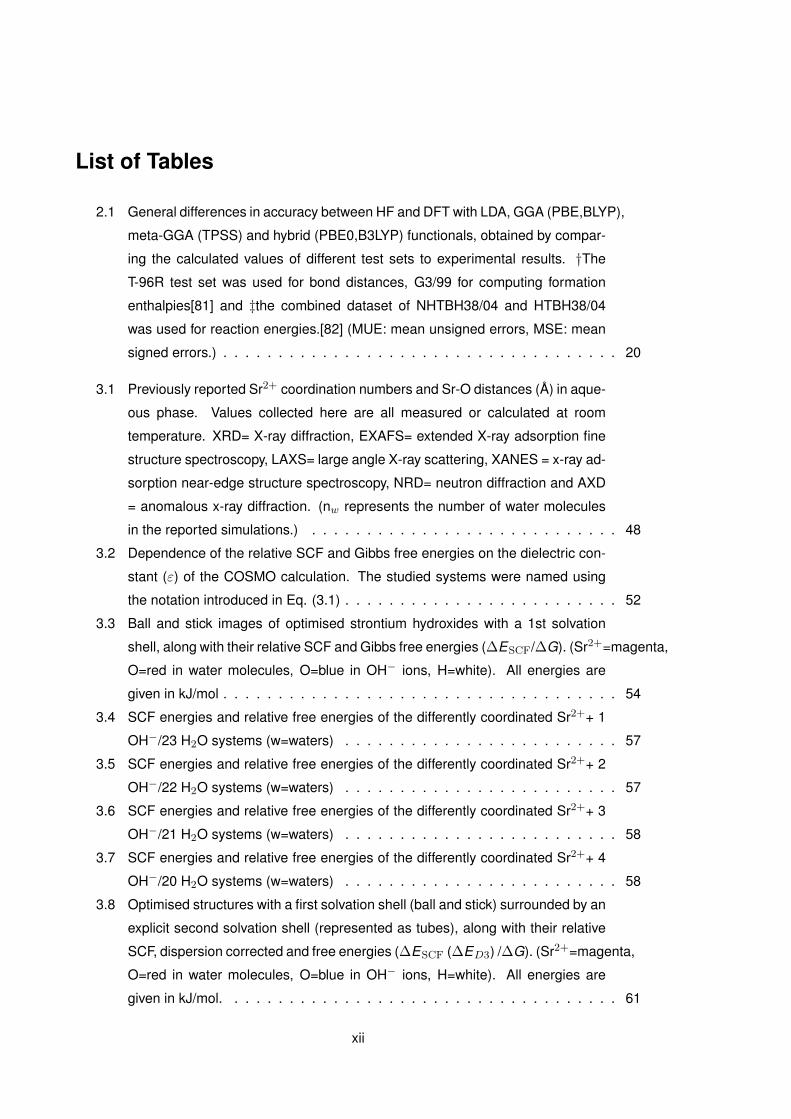
List of Tables
2.1 General differences in accuracy between HF and DFT with LDA, GGA (PBE,BLYP),
meta-GGA (TPSS) and hybrid (PBE0,B3LYP) functionals, obtained by compar-
ing the calculated values of different test sets to experimental results. †The
T-96R test set was used for bond distances, G3/99 for computing formation
enthalpies[81] and ‡the combined dataset of NHTBH38/04 and HTBH38/04
was used for reaction energies.[82] (MUE: mean unsigned errors, MSE: mean
signed errors.) . . . . . . . . . . . . . . . . . . . . . . . . . . . . . . . . . . . . 20
3.1 Previously reported Sr2+ coordination numbers and Sr-O distances (A) in aque-
ous phase. Values collected here are all measured or calculated at room
temperature. XRD= X-ray diffraction, EXAFS= extended X-ray adsorption fine
structure spectroscopy, LAXS= large angle X-ray scattering, XANES = x-ray ad-
sorption near-edge structure spectroscopy, NRD= neutron diffraction and AXD
= anomalous x-ray diffraction. (nw represents the number of water molecules
in the reported simulations.) . . . . . . . . . . . . . . . . . . . . . . . . . . . . 48
3.2 Dependence of the relative SCF and Gibbs free energies on the dielectric con-
stant (ε) of the COSMO calculation. The studied systems were named using
the notation introduced in Eq. (3.1) . . . . . . . . . . . . . . . . . . . . . . . . . 52
3.3 Ball and stick images of optimised strontium hydroxides with a 1st solvation
shell, along with their relative SCF and Gibbs free energies (∆ESCF/∆G). (Sr2+=magenta,
O=red in water molecules, O=blue in OH− ions, H=white). All energies are
given in kJ/mol . . . . . . . . . . . . . . . . . . . . . . . . . . . . . . . . . . . . 54
3.4 SCF energies and relative free energies of the differently coordinated Sr2++ 1
OH−/23 H2O systems (w=waters) . . . . . . . . . . . . . . . . . . . . . . . . . 57
3.5 SCF energies and relative free energies of the differently coordinated Sr2++ 2
OH−/22 H2O systems (w=waters) . . . . . . . . . . . . . . . . . . . . . . . . . 57
3.6 SCF energies and relative free energies of the differently coordinated Sr2++ 3
OH−/21 H2O systems (w=waters) . . . . . . . . . . . . . . . . . . . . . . . . . 58
3.7 SCF energies and relative free energies of the differently coordinated Sr2++ 4
OH−/20 H2O systems (w=waters) . . . . . . . . . . . . . . . . . . . . . . . . . 58
3.8 Optimised structures with a first solvation shell (ball and stick) surrounded by an
explicit second solvation shell (represented as tubes), along with their relative
SCF, dispersion corrected and free energies (∆ESCF (∆ED3) /∆G). (Sr2+=magenta,
O=red in water molecules, O=blue in OH− ions, H=white). All energies are
given in kJ/mol. . . . . . . . . . . . . . . . . . . . . . . . . . . . . . . . . . . . 61
xii

LIST OF TABLES xiii
3.9 The average Sr-Ow and Sr-OOH distances (A) in the first and second solva-
tion shell for Sr2+ hydrates and each type of hydroxide. For simplicity, water
molecules in the third shell are included in the second shell averages. Stan-
dard deviations (SD) are presented in parentheses . . . . . . . . . . . . . . . . 63
3.10 Boltzmann distribution of differently coordinated Sr2+ hydroxide complexes cal-
culated based on the Gibbs free energies at room temperature . . . . . . . . . 64
3.11 SCF (∆ESCF) and Gibbs free energy differences (∆G) of the dihydroxide −→monohydroxide proton transfer reaction. TS = transition state . . . . . . . . . . 65
3.12 Oxygen charges of the dihydroxide ([Sr:4/18:2/0]) and monohydroxide ([Sr:5/17:1/1])
complexes with 22 water molecules calculated by QTAIM analysis. O(OH1)
and O(OH2) are the charges of the oxygen atoms in the hydroxide ions while
the following rows are the average charges and the related standard deviation
calculated for the oxygen atoms in the first and second solvation shell. . . . . . 66
3.13 Relative SCF (∆ESCF) and Gibbs free energies (∆G) in kJ/mol for the reactions
described by Eq. (3.2) and Eq. (3.3),calculated with the def2-TZVP basis set . . 67
3.14 Dependence of SCF energies for Eq. (3.2) on basis set quality. ∆E for the
def2-SVP and def2-TZVP basis sets were calculated compared to the def2-
QZVP results. All energies are in kJ/mol. . . . . . . . . . . . . . . . . . . . . . 67
4.1 Summary of the previously published geometrical properties of brucite. All val-
ues are in A. (a, c are lattice parameters, zO and zH are fractional coordinates;
Mg-O and O-H are bond lengths; H· · ·H and O· · ·O are atomic distances.) . . . 72
4.2 Comparison of the previously published interlayer interaction energies (IE) with
different functionals. The LDA and GGA functionals used vary in the different
studies, but the trend is similar. (a BSSE correction was used in the given study.) 76
4.3 Calculated average d(Mg-O) and d(O-H) bond lengths together with the d(O· ··O) atomic distances of the QM cluster in 6x6 1, compared with the structural
parameters of a previous computational study and experiments. All values are
in A. (SD stands for the standard deviation of the calculated average parameter.) 83
4.4 SCF energies and the RMS deviation of the Mg z coordinates in the systems
with a 6x6 Mg(OH)2 cluster and 0 to 8 PC layers . . . . . . . . . . . . . . . . . 84
4.5 Comparison of SCF energies and RMS deviation of the Mg z coordinates in the
first brucite layer, for systems with more explicit layers within the cluster and
with or without extra PC layers. (nxn refers to the number of Mg atoms in the
cluster, (nxn)’ refers to clusters with modified geometries) . . . . . . . . . . . . 86
4.6 Comparison of SCF energies and RMS deviation of the Mg z coordinates in
the first cluster, for 6x6 2 systems with fixed atomic coordinates in different
positions (with or without extra PC layers) . . . . . . . . . . . . . . . . . . . . . 87

xiv LIST OF TABLES
4.7 Geometrical properties of bulk brucite structure calculated with CRYSTAL, com-
pared to previously published parameters. All values are in A (a, c are lattice
parameters, Mg-O and O-H are bond lengths; H· · ·H and O· · ·O are atomic
distances) aCalculated based on published fractional coordinates (zH , zO) . . . 89
4.8 Calculated surface energies, Mulliken atomic charges and bond populations for
different number of brucite layers in the slab with CRYSTAL. . . . . . . . . . . . 90
4.9 Adsorption energies of a series of s block ions: (1): calculated with Eq. (4.2)
and using a mixed basis set, ion TZVP (def2-TZVP on the ion and def2-SVP
on the surface) (2): with Eq. (4.3) and ion TZVP, and (3): with Eq. (4.3) and
using a modified closed shell basis set on the cation. ∆Eads are the energy
differences between the interaction energies evaluated with different methods.
(3)* represents the adsorption energies calculated with the correction terms
shown in Table 4.10. . . . . . . . . . . . . . . . . . . . . . . . . . . . . . . . . 93
4.10 Estimated energy difference arising due to the truncation of the cation basis
sets, calculated by comparing the energy of a lone ion with full and truncated
basis set. (∆E = Efull-E trunc) . . . . . . . . . . . . . . . . . . . . . . . . . . . 94
4.11 Adsorption energies (Eads) of a series of s block ions and relative adsorption
energies of different surface representations for a given ion, calculated by com-
paring the results to the adsorption energy of the 6x6 1 structures (∆Eads).
Counterpoise corrected energy values are presented in brackets (BSSE). (The
adsorption energies with ion-SVP and ion-TZVP mixed basis sets are not cal-
culated for 6x6 1+PC.) . . . . . . . . . . . . . . . . . . . . . . . . . . . . . . . 95
4.12 Adsorption energies of a series of s block ions on a single layer of brucite
(6x6 1) calculated with def2-SVP, def2-TZVP and def2-QZVP and the adsorp-
tion energy differences between the TZVP/SVP and QZVP/TZVP results. All
values are in kJ/mol.aThe exceptional behaviour of the Mg2+ is explained in
Figure 4.13. . . . . . . . . . . . . . . . . . . . . . . . . . . . . . . . . . . . . . 97
4.13 Adsorption energies (Eads) and relative adsorption energies (∆Eads) of the
Sr2+ hydrate complex with different surface representations. The relative ener-
gies are calculated by comparing the results to the energy of the complex on a
single layer. . . . . . . . . . . . . . . . . . . . . . . . . . . . . . . . . . . . . . 101
4.14 Adsorption energies (Eads) and relative adsorption energies (∆Eads) of the
Sr2+ hydrate complex with different surface representations containing two ex-
plicit 6x6 layers in the QM cluster, fixed atomic positions and 0 or 1 PC layer.
The relative energies are calculated by comparing the results to the energy of
the complex on the fully relaxed 6x6 2 system without a PC layer. (All energies
are calculated with the def2-SVP basis set.) . . . . . . . . . . . . . . . . . . . . 102

LIST OF TABLES xv
4.15 Substitution energies (Esub) calculated with periodic DFT (PBC) and with the
PEECM, including 1 or 2 explicit layers of brucite in the model. The energy
differences between the two models are represented in percentages (Ediff )
relative to the periodic DFT values . . . . . . . . . . . . . . . . . . . . . . . . . 104
4.16 Periodic DFT-calculated substitution energies (Esub) as a function of cell size
for Ca2+ and Sr2+, considering 1,2 and 3 number of brucite layers in the slab.
(aNote that the gradient of the 7x7 3 system did not fully converge (the max
gradient was 0.000501 while the convergence criterion is 0.000450), although
the energy did.) . . . . . . . . . . . . . . . . . . . . . . . . . . . . . . . . . . . 105
4.17 Absolute (Eads) and relative adsorption energies (∆Eads) of four Sr[(OH)2(H2O)4]
complexes, calculated by comparing each system to the most stable structure.
Counterpoise corrected energy values are presented in brackets (BSSE). . . . . 107
4.18 Periodic DFT-calculated adsorption energies (Eads) as a function of cell size for
structure 1-4. A full cell size study was performed for the most stable structure
(3) and cell sizes of 7x7 1, 7x7 2 and 9x9 1 were calculated for the less sta-
ble structures. (aNote that the total energy of structure 2 with 7x7 2 cell size
converged to 10−5 a.u.) . . . . . . . . . . . . . . . . . . . . . . . . . . . . . . . 109
4.19 Periodic DFT-calculated relative adsorption energies (∆Eads) of four [Sr(OH)2(H2O)4]
complexes, calculated by comparing each system to the most stable structure
(3) with different cell sizes (aNote that the total energy of structure 2 with 7x7 2
cell size converged to 10−5 a.u.) . . . . . . . . . . . . . . . . . . . . . . . . . . 109
4.20 Sr-O distances (d) and electron densities at the bond critical points (ρ) for each
coordinated OH group or H2O molecule calculated with QTAIM for the optimised
structures in PEECM or periodic DFT (PBC). R2 is the coefficient of determina-
tion for the linear regression between d and ρ and CN is the total coordination
number. For structures and Sr-O labels see Figure 4.20. (aIn structure 1, there
is a fourth water coordinated to the Sr instead of a fifth OH group.) . . . . . . . 111
4.21 Electron densities at the Sr-O BCPs plotted against Sr-O distances for the four
Sr[(OH)2(H2O)4] complexes optimised with PEECM or periodic DFT (PBC).
Red squares are related to the Sr-O(OH) interactions in the solvation shell,
crossed squares to the Sr-O(H2O) interactions in the solvation shell and black
squares to the Sr-O(surface) interactions with the surface OH groups. . . . . . . 112

xvi LIST OF TABLES
5.1 The inner and outer shell complexes obtained for systems without additional
OH− ion. The relative absorption energies (∆Eads) were calculated by us-
ing Eq. (5.2) along with the reference system [Sr:6/18:0/0]2+ and by com-
paring every structure to the most stable one (C1), OHsurf is the number of
Sr-coordinated OH surface groups in the system, CN is the total coordination
number of the Sr2+ complex and dSr−surf is the cation-surface distancei . . . . 129
5.2 Natural charges of the oxygen atoms for each Sr-coordinated OH surface group
(O(surf)), H2O molecule (O(H2O)) and solvated OH− ion (O(OH)), and the nat-
ural charge of the Sr atom, for the optimised structures in Figure 5.10 and Table
5.1. The average charge together with the corresponding standard deviation
was calculated for the surface oxygen atoms (AVE(surf) and SD(surf)) and the
oxygen atoms in the hydration layers (AVE(hydr) and SD(hydr)). . . . . . . . . . 133
5.3 The inner and outer shell complexes obtained for systems with 2 additional OH−
ions. The relative absorption energies (∆Eads) are calculated by using Eq. (5.2)
along with the reference system [Sr:5/17:1/1] and by comparing every structure
to the most stable one (C1 OH2 1), OHsurf is the number of Sr-coordinated
OH surface groups in the system, CN is the total coordination number of the
Sr2+ complex and dSr−surf is the cation-surface distance. . . . . . . . . . . . . 135
5.4 The inner and outer shell complexes obtained for systems with 1 additional
OH− ion. The relative absorption energies (∆Eads) are calculated by using
Eq. (5.2) along with the reference system [Sr:5/18:1/0]+ and by comparing
every structure to the most stable one (C1 OH1 1, OHsurf is the number of
Sr-coordinated OH surface groups in the system, CN is the total coordination
number of the Sr2+ complex and dSr−surf is the cation-surface distance. . . . . 137
5.5 Dependence of the absolute adsorption energies (kJ/mol) on the basis set qual-
ity of the Sr2+ for systems from Table 5.1, 5.3 and 5.3 calculated with Eq. (5.2).
(Standard deviations calculated for each averages are shown in brackets.) . . . 145
A.1 k mesh convergence for the bulk structure calculations with CRYSTAL. (IS=shrinking
factor in reciprocal space) . . . . . . . . . . . . . . . . . . . . . . . . . . . . . . 180
A.2 k mesh convergence for the 5x5 1 structure calculations with CRYSTAL. (IS=shrinking
factor in reciprocal space) . . . . . . . . . . . . . . . . . . . . . . . . . . . . . . 180
A.3 Calculated SCF energies of the considered supercells in CRYSYAL, including
1,2 and 3 brucite layers in the slab. . . . . . . . . . . . . . . . . . . . . . . . . . 180

Chapter 1
Introduction
Much of the UK’s nuclear legacy wastei has been stored in ponds, wet silos and tanks
which contain a large quantity of radioactive sludge formed by the in-pond corrosion of the
spent Magnox fuel cladding. The composition of the waste is heterogeneous and it can change
with the changing environment, but due to the high biological hazard and the difficulties in
accessing and analysing the old-time paper based records, the monitoring and investigation
of the exact compositions is very difficult. Since the storage facilities are close to the end
of their designed life-time, a decommissioning program was initiated by Sellafield Ltd. to
remove the waste from those facilities with the ultimate aim to immobilise and prepare the
nuclear waste for long-term storage. However, due to the lack of complete understanding of
the conditions of the ponds, the decommissioning is very challenging and requires complex
solutions involving the combination of experimental measurements on simulated systems,
computational modelling and technological developments.[1]
With the improvement of computational technologies, modelling plays a key role in several
stages of the investigation and waste management: it can help to interrogate key process
variables, define future monitoring requirements, underpin operating envelopes and technical
risks. Modelling of fundamental chemical behaviours can help to understand the chemical
reactions, soluble speciation and thermodynamically stable phases existing in the ponds.[2]
The aim of my PhD project is to provide quantum chemical insight into the interactions
between fission generated Sr2+ and hydrated brucite surfaces to help understand the fun-
damental chemistry behind the present conditions in the legacy ponds. To be successful in
this task, first we need to understand the industrial background of the problem by studying
the history of the legacy ponds (1.1), their content (1.2) and the proposed waste treatment
(1.3), then identify the key challenges and objectives for the computational investigation of the
chosen problem (1.4).
iThe objective ”legacy” refers to nuclear waste which was produced during the pioneering nuclear researchand early civil or military nuclear power programmes.
1

2 CHAPTER 1. INTRODUCTION
1.1 The legacy of Magnox reactors
The first British civil nuclear power reactors were Magnox-type which were pressurised,
carbon-dioxide cooled systems with graphite moderators. The fuel contained unenriched
uranium metal encased in a magnesium-aluminium alloy, called Magnox (Magnesium non-
oxidising, represented in Figure 1.1a.[3] The exact composition of the alloy could vary de-
pending on reactor site, but the magnesium content was usually up to 90% and, in addition to
other elements with very small concentration (e.g. Be, Ca, Zr, Fe ...), the aluminium concen-
tration changed from less than 0.02 up to 0.9%.[4] The key advantage of this specific alloy was
its relatively low neutron capture cross section, which made it applicable as neutron moderat-
ing, neutron reflecting cladding material. However, it could be used only at a limited maximum
operating temperature, due to possible secondary recrystallisation and significant changes in
the grain structure at high temperatures,[5, 6] which seriously limited the thermal efficiency of
this type of reactor.
(a) Oldbury Magnox fuel element ingraphite brick[7] (b) Opened air legacy pond in Sellafield[8]
Figure 1.1: Example of a nuclear legacy pond and a Magnox-type fuel element
During the second part of the twentieth century, 26 Magnox reactors were built in the UK,
most of them with slightly different designs[3, 9] and with modified Magnox compositions.[4]
None of these is operating any more; the last of the Magnox-type reactors in Britain, Wylfa,
was shut down in 2015. The used fuel rods and cladding material became part of the interme-
diate and high level nuclear waste (ILW and HLW)[10] and are currently stored in fuel storage
ponds and wet silos in Sellafield and other reactor sites in the country. ILW materials still pro-
duce significant amounts of radiation, but not as much as HLWs which are so radioactive that
the generated heat by these materials has to be taken into account during their storing period.
Therefore the spent Magnox fuel rods are stored temporarily in ponds or other facilities, filled
with water to act as a radioactivity shield and as a cooling medium, before final disposal or
reprocessing. In some facilities, such as the one in Figure 1.1b, spent fuel has been stored
1.1. THE LEGACY OF MAGNOX REACTORS 3
for decades and this material represents a hazard that needs to be addressed.
Another disadvantage of Magnox is its reactivity with water. More accurately, Magnox
corrosion is accelerated by the presence of chloride in the pond water. Although NaOH is
used to maintain the high pH, since the legacy ponds are opened to the air near to the coast,
a chloride build-up from sea-salt aerosols and insufficient purging of the water has resulted
in the corrosion of the cladding material during the long period of storage. The magnesium-
aluminium alloy has corroded during the years of storage under water, and formed a large
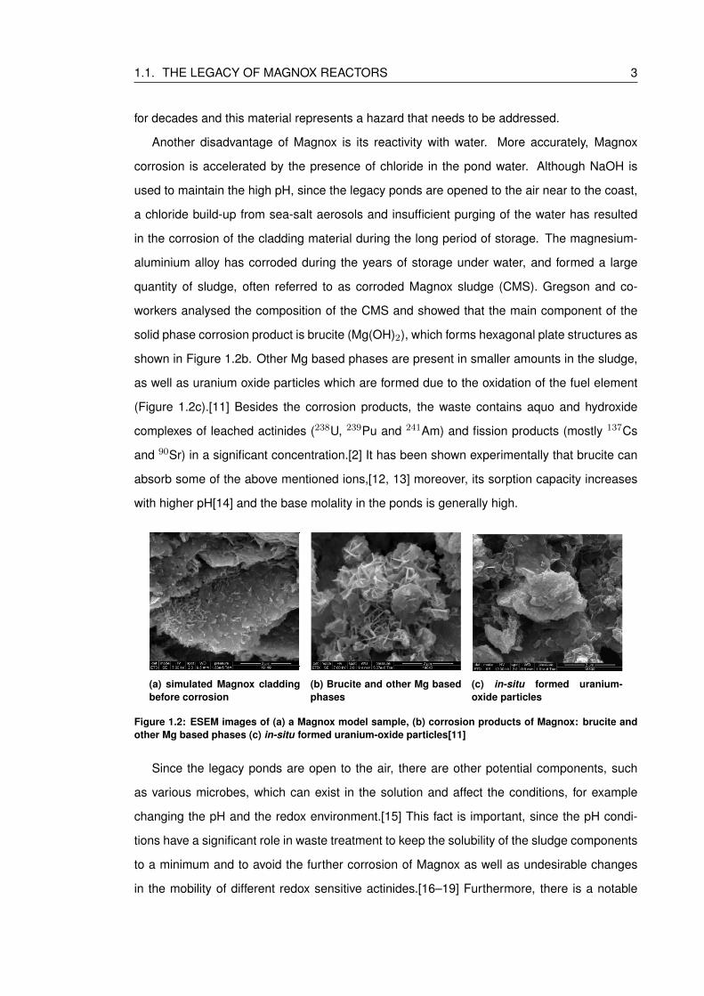
quantity of sludge, often referred to as corroded Magnox sludge (CMS). Gregson and co-
workers analysed the composition of the CMS and showed that the main component of the
solid phase corrosion product is brucite (Mg(OH)2), which forms hexagonal plate structures as
shown in Figure 1.2b. Other Mg based phases are present in smaller amounts in the sludge,
as well as uranium oxide particles which are formed due to the oxidation of the fuel element
(Figure 1.2c).[11] Besides the corrosion products, the waste contains aquo and hydroxide
complexes of leached actinides (238U, 239Pu and 241Am) and fission products (mostly 137Cs
and 90Sr) in a significant concentration.[2] It has been shown experimentally that brucite can
absorb some of the above mentioned ions,[12, 13] moreover, its sorption capacity increases
with higher pH[14] and the base molality in the ponds is generally high.
(a) simulated Magnox claddingbefore corrosion
(b) Brucite and other Mg basedphases
(c) in-situ formed uranium-oxide particles
Figure 1.2: ESEM images of (a) a Magnox model sample, (b) corrosion products of Magnox: brucite andother Mg based phases (c) in-situ formed uranium-oxide particles[11]
Since the legacy ponds are open to the air, there are other potential components, such
as various microbes, which can exist in the solution and affect the conditions, for example
changing the pH and the redox environment.[15] This fact is important, since the pH condi-
tions have a significant role in waste treatment to keep the solubility of the sludge components
to a minimum and to avoid the further corrosion of Magnox as well as undesirable changes
in the mobility of different redox sensitive actinides.[16–19] Furthermore, there is a notable
4 CHAPTER 1. INTRODUCTION
CO2 dissolution in the open ponds over time. The dissolved CO2 can induce significant struc-
tural changes, e.g. the transformation of the brucite to various Mg hydrocarbonate phases or
carbonate complexation of the actinide ions in solution.[20, 21]
1.2 Hazardous radioactive ions in the ponds
The unenriched uranium metal contains a combination of three isotopes (0.711% 235U,
99.284% 238U and 0.0055% 234U). When it is used as fuel for thermal reactors, 238U captures
one slow neutron and after two beta decaying steps becomes fissile 239Pu. 235U and 239Pu,
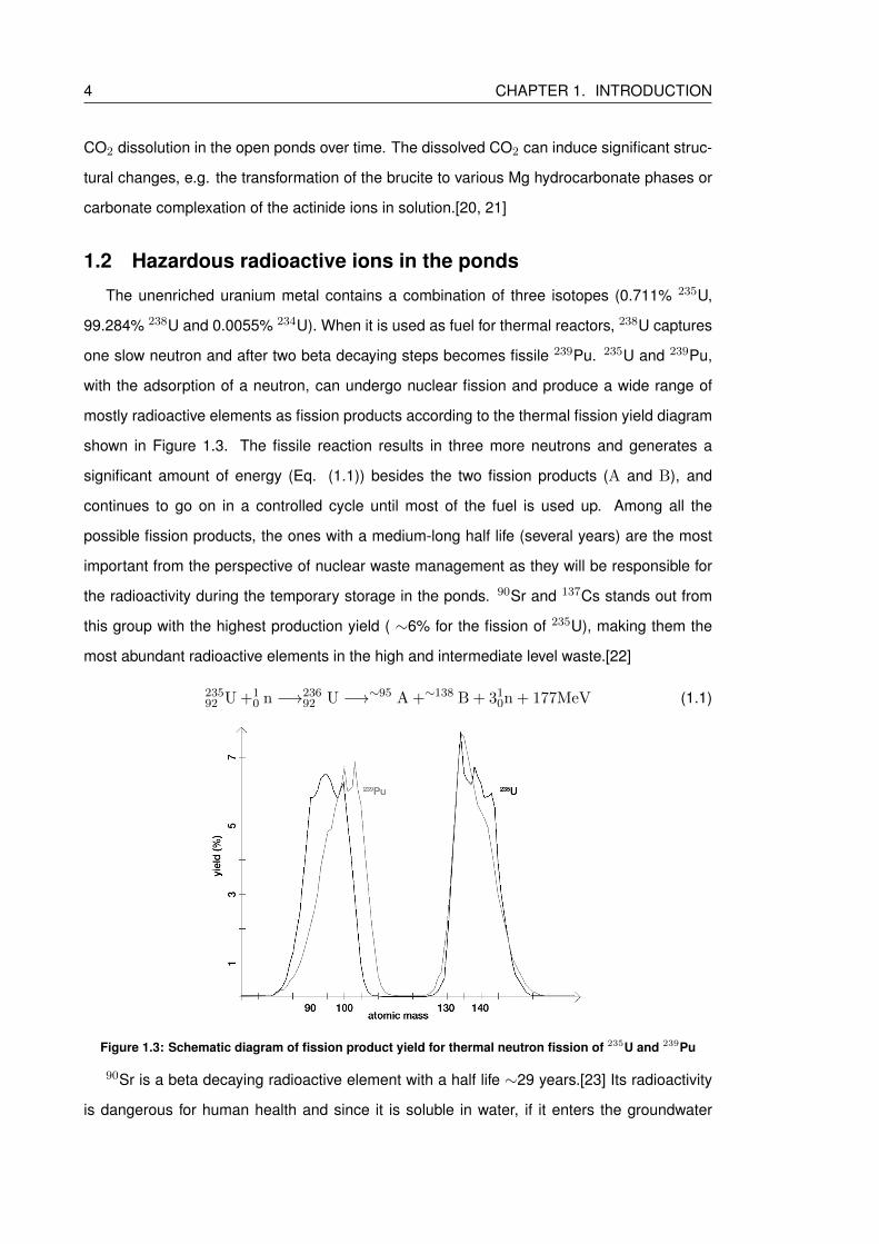
with the adsorption of a neutron, can undergo nuclear fission and produce a wide range of
mostly radioactive elements as fission products according to the thermal fission yield diagram
shown in Figure 1.3. The fissile reaction results in three more neutrons and generates a
significant amount of energy (Eq. (1.1)) besides the two fission products (A and B), and
continues to go on in a controlled cycle until most of the fuel is used up. Among all the
possible fission products, the ones with a medium-long half life (several years) are the most
important from the perspective of nuclear waste management as they will be responsible for
the radioactivity during the temporary storage in the ponds. 90Sr and 137Cs stands out from
this group with the highest production yield ( ∼6% for the fission of 235U), making them the
most abundant radioactive elements in the high and intermediate level waste.[22]
23592 U +1
0 n −→23692 U −→∼95 A +∼138 B + 31
0n + 177MeV (1.1)
Figure 1.3: Schematic diagram of fission product yield for thermal neutron fission of 235U and 239Pu
90Sr is a beta decaying radioactive element with a half life ∼29 years.[23] Its radioactivity
is dangerous for human health and since it is soluble in water, if it enters the groundwater

1.3. SIXEP: THE POND WATER TREATMENT PROCESS 5
or soil,[15, 24] it carries a major hazard for the environment. 90Sr can be inhaled too, but
ingestion in food and water is the greatest health concern. Because the biochemical behaviour
of Sr is very similar to Ca, it deposits in the bones, teeth and bone marrow and can cause
cancer there and in the surrounding soft tissues. [25–27] 137Cs emits both beta particles and
gamma rays with a half life of 30 years.[23] It also travels easily through air and is soluble
in water, however, it is less likely to move in the ground than 90Sr, as it bonds strongly to
the soil.[26] 137Cs is most dangerous through external exposure to a large amount due to its
gamma radiation, but it hardly occurs in such a high concentration. When it enters the body
it gets more or less uniformly distributed with the highest concentration in the soft tissues and
increases the risk of cancer.[26]
The deposited used fuel rods still contain a high amount of solid uranium (>95%), which
can also be partially released in the solution, along with to solvated ions of other alpha emitting
by-products of the fissile/neutron capture reactions, such as different isotopes of Pu, Am and
Cm.[28] The uranium most likely becomes UO2+2 when it corrodes and it can be present both
in the solid and aqueous phase of the waste.
1.3 SIXEP: the pond water treatment process
Filtration and ion exchange treatment plants are typically used to condition waste water
prior to discharging, such as the Site Ion eXchange Effluent Plant (SIXEP) which has oper-
ated in Sellafield since 1985 and is used to remove almost all the radioactivity of the liquid
effluent from the storage ponds before sea discharge.[29] The feed entering the SIXEP plant
is quite heterogeneous: it is an alkaline (pH > 11) water solution containing solid materials
with various particle sizes and a range of mobile ions; of which the radioactive ones are pri-
marily 90Sr and 137Cs, but some alpha emitting actinides too (e.g. Pu, 241Am, 242Cm and
244Cm)[28]. There is also a large concentration of non-radioactive cations, mostly Na+ Mg2+,
Ca2+ and K+.[2] The concentration of the latter ions is an important factor as these ions are
competitors of the radioactive solutes in the cation exchange process.
A schematic flow chart of the SIXEP operating in the Sellafield site is shown in Figure
1.4. Although the heart of the process are the ion exchange beds where the radioactive (and
the non-radioactive) cations are swapped with cations of the ion exchanger material (usually
some kind of zeolite e.g. clinoptilolite which is a natural zeolite particularly selective for Sr
and Cs ions[2]), the feed has to go through several treatment processes before entering the
ion exchange columns.[2, 30] First, the suspended solids have to be removed by settling and

6 CHAPTER 1. INTRODUCTION
filtration to avoid blocking the beds and to take away a significant amount of activity linked
to the solid phase. Settling tanks are used to remove larger particulates and experimental
results with simulated sludge have showed a significant strontium uptake at this step (by the
solid phase) which was initially linked to the presence of brucite. In the reception tank, poly-
electrolytes are added to the feed to enhance the filtration of smaller particles and colloids by
the sand bed filters. 90% of the alpha emitters (Am and Cm) are filtered out at this point as
they mostly sorb onto solid particulates, however Pu ions are less likely to absorb and there-
fore they are detected with an almost unaltered concentration at the end of this process.[28]
The next step is the carbonation tower, where the entering alkaline liquor contacts with carbon
dioxide and forms carbonates and hydrocarbonates while the pH reduces to close to neutral.
Figure 1.4: The process diagramm of SIXEP[2]
The ion exchange columns have a certain ion exchange capacity which is supposed to be
constant and determined only by the number of functional groups available for ion exchange
in the material. However, in the process design and operational point of view, the so-called
breakthrough capacity is a more important factor, as it is refers to the volume of solution which
can be treated in the plant before the concentration of the radioactive ions starts to increase in
the leaving effluent.[31] It depends on several variables, such as the initial ion concentration
of the entering liquor, ionic size and valence, temperature, nature of the functional group
etc.; and once this volume is achieved, the used ion exchanger has to be physically removed
from the vessels, disposed as solid radioactive waste and replaced with new material. In the
case of uncertain feed composition, the SIXEP process has to run within big safety limits,
assuming the highest possible concentration of movable ions, which can be extremely costly
and inefficient, Besides the fact that the ion exchange beds are also part of the radioactive
waste, there is a limited storage place for them, and during their replacement the SIXEP runs

1.4. COMPUTATIONAL CHALLENGES 7
only with half-capacity; all of these are good reasons to continue the investigation on the exact
feed composition.
1.4 Computational challenges
Brucite, as the main corrosion product of the cladding material, coexists with radioactive
solvated ions, such as the fission generated Sr2+, in an alkaline aqueous solution in the
ponds. When this solution enters the SIXEP plant for treatment, the solid phase is separated
from the liquid phase. A significant but not constant strontium uptake is detected at this point
and for the optimal operation of the plant, it is crucial to understand what is responsible for
this uptake. If there are strong interactions between the Sr2+ ion and the solid Mg(OH)2, a
significant concentration of strontium may stay in the solid waste form sorbed to the brucite,
leaving a lower concentration in the effluent entering the ion exchange beds.
Computational studies have been used on several occasions to provide insight into ion/sur-
face interactions at the molecular level by predicting preferred reaction sites,[32–36] calculat-
ing the most stable structures during the interactions[35, 37–39] and allowing comparison of
the interaction energies of competing species[40–42]. Moreover, there are several examples
in the literature in which simulations have helped to improve our knowledge of radionuclide
related transport mechanisms in minerals[43] by determining the strength and type of their
interaction with transport media, such as molecular dynamics studies of the interaction of
solvated uranyl ions with common soil components around nuclear waste depositories,[35,
44–47] and computational investigations of ionic transport mechanisms in the filtration media
used during the decommissioning process such as sand and zeolite type ion exchangers[48,
49].
For this particular problem, first we have to know the thermodynamically stable complexes
of the Sr2+ in a high pH environment and create a model capable of studying the energetics of
ionic adsorption on a water/solid interface, to be able to investigate the proposed interactions
between Sr and brucite.
1.4.1 Studying the hydrolysis of Sr2+ in aqueous environment
Although the speciation of Sr(OH)2 in alkaline conditions and changing temperatures had
been studied experimentally, there is no structural information on the geometry of the thermo-
dynamically stable Sr2+ complexes in solution. With very few exceptions, hydrolysis constants
are determined from pH-dependent solubility studies[50] or recently by AC conductivity mea-
surements.[51] Therefore, as a first step of this PhD project, we have to identify the thermody-

8 CHAPTER 1. INTRODUCTION
namically stable Sr2+ species in the solution to be able to use them as candidate species for
the interactions and as reference structures representing the solvated complexes in the bulk
solvent.
Modelling solvation or ligand exchange in solvated complexes with quantum chemical
methods requires different approaches than reactions involving strong chemical bonds, be-
cause these complexes are generally formed by weak and labile bonds where the effects of
the solvent-solute interactions cannot be neglected.[52] Thus, in addition to the selection of
an appropriate computational method and basis set, several other factors such as the con-
tinuum solvent model and the explicit inclusion of the first or even second solvation shells
can have a significant effect on the results and have to be carefully considered during the
investigation.[53] Chapter 3 of this thesis explains the work which has been carried out on this
subject.
1.4.2 Creating a suitable surface representation of (0001) brucite surface
An important challenge for the project is to create a suitable brucite model for the proposed
interaction. However, choosing a surface representation for the investigation of a particular
adsorption mechanism is not always straightforward, and the choice can heavily influence the
outcome of the results. One of the most common approaches to model surfaces is periodic
density functional theory (DFT)[54], which operates with conventional unit cells and employs
periodic boundary conditions. One popular alternative to modelling a surface with periodic
DFT is to use embedded cluster methods to represent an isolated adsorption site on a periodic
surface.[55–57]
For the given problem, we have to consider the following aspects before we decide on
the surface model: for the sake comparability and continuity within the thesis, the developed
system has to be compatible with previous results on the solvated Sr2+ complexes, and has to
have the capability to contain at least the same number of water molecules above the surface
as it is used in the solvation study. The model has to work for the adsorption of charged
species too and has to be able to describe the energetics of adsorption interactions on the
surface. Last but not least, ideally it should have moderate computational requirements to be
possibly used in other nuclear industry related problems in the future. Our choice of modelling
method and the steps toward surface optimisation and validation is the topic of chapter 4.

1.4. COMPUTATIONAL CHALLENGES 9
1.4.3 Studying the interactions between the solvated Sr2+ and hydrated (0001)
brucite surface
The typical experimental studies which are carried out on simulated CMS, are measuring
the activity released from the sludge before and after the separation of the solid content and
calculating the activity release fraction (RF), the distribution coefficient (Kd) and the sorption
capacity in percentage based on the results.[15] Besides the changing content of the sludge,
many variables, such as the pH and temperature, can affect the interactions between ions and
solids and it is hard to differentiate and prioritise between these factors. Quantum chemical
calculations allow us an insight for the same absorption reactions from another, atomic-scale,
perspective in which we can investigate the preferred structures of the absorbed complexes
as well as the energetics and chemical background of the detected interactions; and ulti-
mately provide important complementary information for the understanding of the measured
behaviours.
Although there are several difficulties which limit the level of complexity that can be achieved
in a quantum chemical model system, in chapter 5 we combine the results and conclusions of
the two previous chapters to create a model as realistic as possible for the Sr adsorption on a
hydrated brucite surface. Then we pursue the investigation by identifying possible structures
for the absorbed complexes, calculating their adsorption energies and, after the careful anal-
ysis of the obtained results, by finally concluding on the theoretical possibility of Sr absorption
on brucite.

Chapter 2
Electronic Structure Theory
a·b This thesis is entirely computational and involves the use of several different methods
and theories. Therefore, in the first part of this chapter I attempt to summarise the basic
ideas of electronic structure theory by first introducing the main approximations of quantum
chemistry and the basics of Hartree-Fock theory, then continue with the density functional
theory and related topics such as functionals and basis sets. More detailed descriptions can
be found in the literature that I used as a basis for this summary.[58–60] In the second part I
concentrate on specific methods which are relevant for this work, such as solvent models and
periodic simulations, while in the last part of the chapter I write about the practical use of the
previously introduced theories.
2.1 The Schrodinger equation and other approximations
In electronic structure calculations one always seeks an approximate solution for the non-
relativistic time-independent Schrodinger equation (SE) shown in Eq. (2.1). The time-independ-
ent SE is an approximation itself, since it assumes that the wavefunction is invariant to time
and ignores relativistic effects. The Dirac equation is a variation of the SE which is consistent
with the theory of relativity, however, due to its complexity, when relativistic effects can be
ignoredi, the solution of SE is the base of most electronic structure theories.
Eq. (2.1) is an eigenvalue problem, which can be solved based on the variational princi-
ple (Eq. (2.2)). H is the Hamiltonian, a Hermitian operator which acts on the ground state
wavefunction (Ψ0(τττ)) and results in the total energy of the system in the ground state, E0 (i.e.
the eigenvalue of the equation) as the expectation value of H with respect to the normalised
wavefunction.
HΨ(τττ) =[Te + Tn + Vne + Vee + Vnn
]Ψ(τττ) = EΨ(τττ) (2.1)⟨
Ψ(τττ)|H|Ψ(τττ)⟩≥ E0 if 〈Ψ(τττ)|Ψ(τττ)〉 = 1 (2.2)
The Hamiltonian includes the following terms (showed in Eq. (2.3) in atomic units): the kinetic
energy operator of N electrons (Te), the kinetic energy operator of M nuclei (Tn) and the po-
iRelativistic effects in the first three periods of the Periodic Table are negligible.
10
2.1. THE SCHRODINGER EQUATION AND OTHER APPROXIMATIONS 11
tential energy operators describing the nucleus-electron attraction (Vne), the electron-electron
(Vee) and nucleus-nucleus repulsion (Vnn) interactions. In the extended form of H riA is the
distance between the electron i and nucleus A, rij is the distance between electron i and j
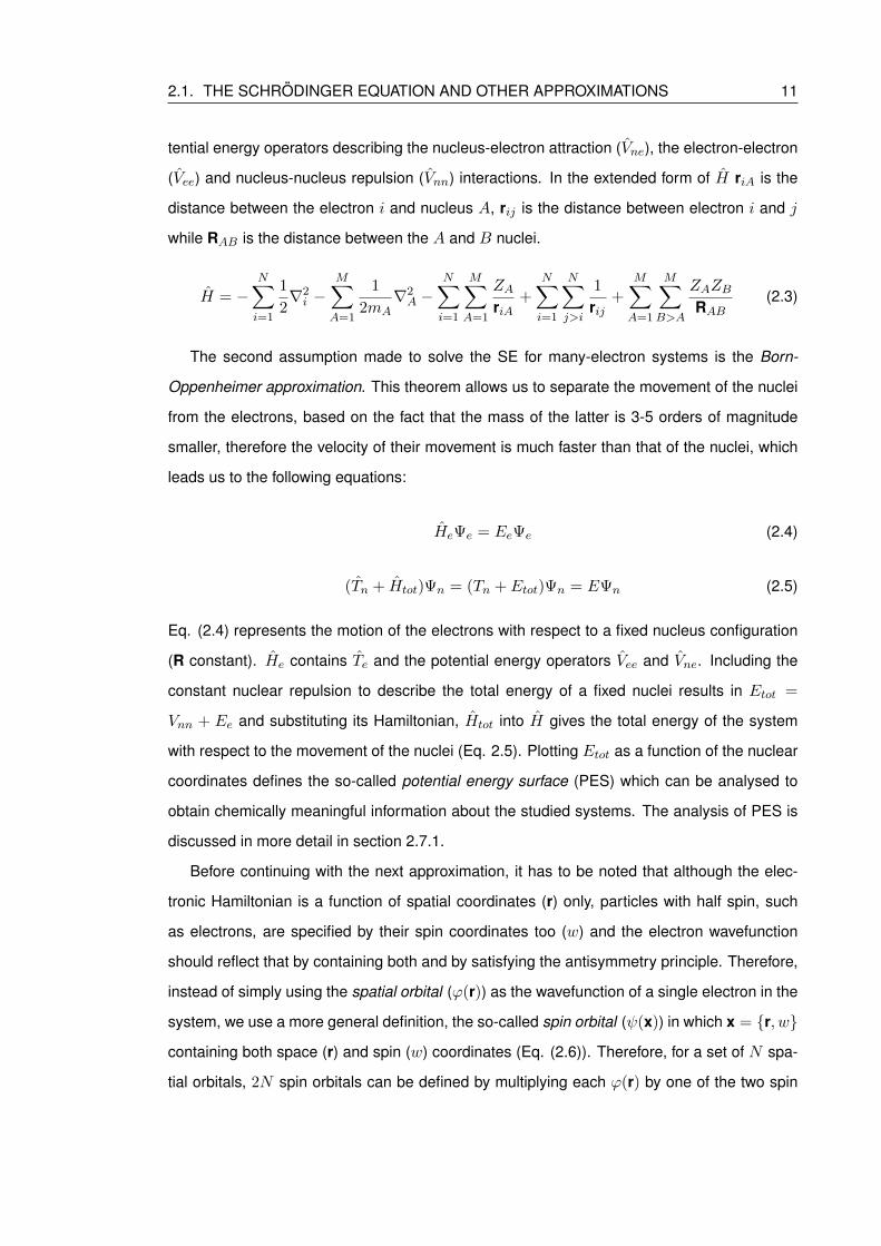
while RAB is the distance between the A and B nuclei.
H = −N∑i=1
1
2∇2i −
M∑A=1
1
2mA∇2A −
N∑i=1
M∑A=1
ZAriA
+N∑i=1
N∑j>i
1
rij+
M∑A=1
M∑B>A
ZAZBRAB
(2.3)
The second assumption made to solve the SE for many-electron systems is the Born-
Oppenheimer approximation. This theorem allows us to separate the movement of the nuclei
from the electrons, based on the fact that the mass of the latter is 3-5 orders of magnitude
smaller, therefore the velocity of their movement is much faster than that of the nuclei, which
leads us to the following equations:
HeΨe = EeΨe (2.4)
(Tn + Htot)Ψn = (Tn + Etot)Ψn = EΨn (2.5)
Eq. (2.4) represents the motion of the electrons with respect to a fixed nucleus configuration
(R constant). He contains Te and the potential energy operators Vee and Vne. Including the
constant nuclear repulsion to describe the total energy of a fixed nuclei results in Etot =
Vnn + Ee and substituting its Hamiltonian, Htot into H gives the total energy of the system
with respect to the movement of the nuclei (Eq. 2.5). Plotting Etot as a function of the nuclear
coordinates defines the so-called potential energy surface (PES) which can be analysed to
obtain chemically meaningful information about the studied systems. The analysis of PES is
discussed in more detail in section 2.7.1.
Before continuing with the next approximation, it has to be noted that although the elec-
tronic Hamiltonian is a function of spatial coordinates (r) only, particles with half spin, such
as electrons, are specified by their spin coordinates too (w) and the electron wavefunction
should reflect that by containing both and by satisfying the antisymmetry principle. Therefore,
instead of simply using the spatial orbital (ϕ(r)) as the wavefunction of a single electron in the
system, we use a more general definition, the so-called spin orbital (ψ(x)) in which x = r, w
containing both space (r) and spin (w) coordinates (Eq. (2.6)). Therefore, for a set of N spa-
tial orbitals, 2N spin orbitals can be defined by multiplying each ϕ(r) by one of the two spin
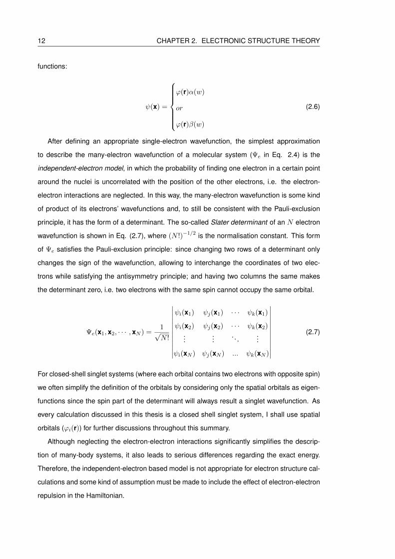
12 CHAPTER 2. ELECTRONIC STRUCTURE THEORY
functions:
ψ(x) =
ϕ(r)α(w)
or
ϕ(r)β(w)
(2.6)
After defining an appropriate single-electron wavefunction, the simplest approximation
to describe the many-electron wavefunction of a molecular system (Ψe in Eq. 2.4) is the
independent-electron model, in which the probability of finding one electron in a certain point
around the nuclei is uncorrelated with the position of the other electrons, i.e. the electron-
electron interactions are neglected. In this way, the many-electron wavefunction is some kind
of product of its electrons’ wavefunctions and, to still be consistent with the Pauli-exclusion
principle, it has the form of a determinant. The so-called Slater determinant of an N electron
wavefunction is shown in Eq. (2.7), where (N !)−1/2 is the normalisation constant. This form
of Ψe satisfies the Pauli-exclusion principle: since changing two rows of a determinant only
changes the sign of the wavefunction, allowing to interchange the coordinates of two elec-
trons while satisfying the antisymmetry principle; and having two columns the same makes
the determinant zero, i.e. two electrons with the same spin cannot occupy the same orbital.
Ψe(x1, x2, · · · , xN ) =1√N !
∣∣∣∣∣∣∣∣∣∣∣∣
ψi(x1) ψj(x1) · · · ψk(x1)
ψi(x2) ψj(x2) · · · ψk(x2)...
.... . .
...
ψi(xN ) ψj(xN ) ... ψk(xN )
∣∣∣∣∣∣∣∣∣∣∣∣(2.7)
For closed-shell singlet systems (where each orbital contains two electrons with opposite spin)
we often simplify the definition of the orbitals by considering only the spatial orbitals as eigen-
functions since the spin part of the determinant will always result a singlet wavefunction. As
every calculation discussed in this thesis is a closed shell singlet system, I shall use spatial
orbitals (ϕi(r)) for further discussions throughout this summary.
Although neglecting the electron-electron interactions significantly simplifies the descrip-
tion of many-body systems, it also leads to serious differences regarding the exact energy.
Therefore, the independent-electron based model is not appropriate for electron structure cal-
culations and some kind of assumption must be made to include the effect of electron-electron
repulsion in the Hamiltonian.
2.2. HARTEE-FOCK THEORY (HF) 13
2.2 Hartee-Fock theory (HF)
In Hartree-Fock theory, one derives the total electronic energy of the ground state by solv-
ing eigenvalue problems, as shown in Eq. (2.8), for each of its electrons. These single-electron
equations are called Hartree-Fock equations[61, 62] and they take into account the electron-
electron interactions by an effective potential (υHFi ) which is the average potential experienced
by the ith electron due to the other electrons present around it.
fiϕi = εiϕi (2.8)
fi = hi + υHFi =1
2∇2i −
M∑A=1
ZAriA
+ υHFi (2.9)
In the HF equations, fi is the one-electron Fock operator containing the Hamiltonian of a
single electron in the field of the nuclei and the effective potential. υHFi contains two operators
(υHFi =∑N
j (Jj − Kj)), which both depend on the coordinates of two electrons and have the
following expectation value with respect to the orbital ϕi:
⟨ϕi(r1)|Jj |ϕi(r1)
⟩=
∫ϕi(r1)∗ϕj(r2)∗
(1
rij
)ϕi(r1)ϕj(r2)dr1dr2 = Jij (2.10)
⟨ϕi(r1)|Kj |ϕi(r1)
⟩=
∫ϕi(r1)∗ϕj(r2)∗
(1
rij
)ϕj(r1)ϕi(r2)dr1dr2 = Kij (2.11)
Jj is the Coulomb operator, it represents the averaged classical repulsion potential acting on
the electron in orbital ϕi at position r1 from the electron in orbital ϕj . Kj is the exchange
operator, its name is coming from the fact that in Kj the spin orbital ϕj exchanges with ϕi
to the right of r−1ij . The exchange potential is the consequence of the antisymmetry princi-
ple: electrons of the same spin cannot occupy the same orbital which reduces the classical
Coulomb repulsion term with a non-classical contribution. It is a non-local operator, i.e. the
value of Kjϕi(r1) depends on the value of ϕi throughout all space. It is easy to see that in
case of i = j, Jii is completely cancelled out by Kii, thus there is no error arising from the
electron interacting with itself.
The HF equations can be solved by using the variational principle, i.e. the energy of the
orbital (εi) is the expectation value of the Fock operator with respect to the normalised orbital,
ϕi. By separating fi to its above described terms (Eq. (2.9), (2.10) and (2.11)) and applying
the variational principle to each, we get the following solution for εi:
14 CHAPTER 2. ELECTRONIC STRUCTURE THEORY
εi = hii +
N∑j
(Jij −Kij) (2.12)
Going back to the original assumption of the HF theory, the energy of the many-electron wave-
function is described as the sum of the orbital energies with a correction term (Eq. (2.13));
one has to subtract half of the interatomic terms, since applying a double sum (∑
i
∑j) on
(Jij −Kij) would count the electron-electron interactions twice. By adding the energy of the
constant nuclear-nuclear repulsion potential to Eq. (2.13), we can calculate the total energy
of the system too: Etot = Ee + Vnn.
Ee =N∑i
εi −1
2
N∑i
N∑j
(Jij −Kij) =N∑i
hii +1
2
N∑i
N∑j
(Jij −Kij) (2.13)
The solution of the HF equations may seem straightforward at first, but one can easily
see that the definition of the Fock operator contains the orbital itself. Therefore, it can only
be solved iteratively, assuming the Fock operator is constructed from a trial set of orbitals
first. Then, a new set of orbitals can be obtained by solving the HF eigenvalue equations
which we can use to construct new fi operators until the orbitals within the Fock operators
are sufficiently close to be the same to the eigenfunctions, i.e. self-consistency is achieved.
Even with the above described self-consistent field method (SCF) in theory there is an infinite
number of possible solutions for the HF equations, as the exact form of the single-electron
wavefunction is unknown. Practically, to limit the number of possible solutions, we expand the
molecular orbital of the system with a linear combination of a finite set of basis functions (χα
in Eq. (2.14)) which often have a form similar to the atomic orbitals (see more in section 2.4).
ϕi =∑α
ciαχα (2.14)
In this approach, which is also known as the Hartree-Fock-Roothaan method,[63] instead of
the basis functions or orbitals, one can vary only the linear coefficients of the basis functions
(ciα) during the iteration process.
In theory, the more sophisticated the basis set, the lower the ground state energy is, i.e. it
becomes closer to the true ground state energy. However, even with a theoretically complete
basis set, there is a known limit of the ground state energy (the Hartree-Fock limit) due to the
errors arising from the averaged electron-electron interactions in the HF approach. Although

2.3. DENSITY FUNCTIONAL THEORY (DFT) 15
relativistic effects can play an important role for heavy elements, typically, the biggest source of
error is the assumption of an average potential field arising from the surrounding electrons. In
fact, HF theory neglects the electron correlation.ii Therefore, to obtain more realistic energies,
one has to use methods which include some kind of electron correlation description in their
model, such as post-Hartree Fock theories or Density Functional Theory.
2.3 Density Functional Theory (DFT)
The advantage of DFT calculations compared to other quantum chemical methods is the
combination of acceptable accuracy and modest computational cost. This has made the DFT
method popular worldwide in quantum chemistry since the 1990s.[64, 65] While there are
serious limitations in accuracy in the Hartree-Fock theory, in most post-HF theories solving
the Schrodinger equation is a difficult many-body problem and the potential depends on the
coordinates of all the interacting electrons. The key feature of the DFT is that in this case, one
solves the Schrodinger equation as a non-interacting problem where the potential is a function
of the electron density i.e. of three space coordinates.iii
But what does the electron density represent? It is a probability density (ρ(r)) which de-
scribes the possibility of finding any electron in a given volume. If one integrates the electron
density (ρ(r)) over the three dimensional space coordinates (r), one will get the number of
electrons (N ) in that volume: ∫ρ(r)dr3 = N (2.15)
The first Hohenberg-Kohn theorem[66] states that the electron density in the ground state
uniquely determines the potential up to an arbitrary constant. It means that ρ(r) can be used
to characterise a system and so we can describe the ground state energy as the functional
of the electron density. Based on this, the total energy of the system can be written in the
following form:
E[ρ(r)] = T [ρ(r)] + Vee[ρ(r)] + Vext[ρ(r)] = F [ρ(r)] +
∫νext(r)ρ(r)dr (2.16)
E[ρ(r)] = T [ρ(r)] + J [ρ(r)] +K[ρ(r)] + Vne[ρ(r)] (2.17)
iiHF does not completely neglect the electron correlation, since the basic correlation of electrons with parallelspin, that they cannot occupy the same space, is included in the exchange term.
iiiThis is true for Kohn-Sham DFT, but not for Hohenberg-Kohn DFT which does not require any Schrodingertype equations. Besides, there is a spin dependence on the potential, which increases the number of variables tofour, but as the calculations reported here are all on closed shell singlet species, I will not discuss spin-polarisedDFT.
16 CHAPTER 2. ELECTRONIC STRUCTURE THEORY
Where E[ρ(r)] is the functional of the total energy of the system and T [ρ(r)] is the kinetic
energy functional of the electrons. Vee[ρ(r)] is the energy functional of repulsion between the
electrons, and just like in the HF theory, it is separated to two terms: Coulomb J [ρ(r)] and
exchange parts K[ρ(r)]. Vext[ρ(r)] is the energy functional of the external potential, which, in
most cases, equals to the Coulomb attraction of the nuclei: Vext[ρ(r)] = Vne[ρ(r)].
We can rewrite equation (2.16) using two terms: one, which is invariant to the external
potential (F [ρ(r)] = T [ρ(r)]+Vee[ρ(r)], universal functional of the density), and another which
depends on it. The second Hohenberg-Kohn theorem states that there is a single F [ρ(r)]
which is different and exact for each electronic system and the exact ground state energy
E0[ρ(r)] and electron density for a given external potential are obtained by minimising E[ρ(r)]
with respect to the density with the number of electrons held constant. The Hohenberg-Kohn
theorems laid down the basic rules of DFT but did not make it an easy-to-solve computational
method, since we still do not know the exact form of F [ρ(r)].
In early models, all energy components were expressed as a functional of the electron den-
sity (orbital-free DFT). Using the classical definition of the Coulomb interactions, the Coulomb
part of electron-electron repulsion (2.18) and the attraction of the nuclei (2.19) can easily
described in this way:
J [ρ(r)] =1
2
∫ ∫ρ(r)ρ(r’)| r− r’ |
drdr’ (2.18)
Vne[ρ(r)] = −Nnuclei∑
a
∫Za(Raρ(r))| Ra − r |
dr (2.19)
However, for the kinetic energy functional and the exchange part of Vee[ρ(r)] there is no
exact definition with the electron density function as we know of, therefore, some assumptions
have to be made. The Thomas-Fermi-Dirac model [67–69] uses the density of the uniform
electron gas (a model which assumes that the electrons are homogeneously distributed in
space) to evaluate these terms with the following equations:
T [ρ(r)] = AF
∫ρ5/3u (r)dr (2.20)
K[ρ(r)] = −AX∫ρ4/3u (r)dr (2.21)
Where AF and AX are constants and ρu(r) is the density of the uniform electron gas. Con-
sidering electrons as homogeneously distributed particles may work for valence electrons in
certain metallic systems, but gives a very poor description of atoms and molecules. In fact,
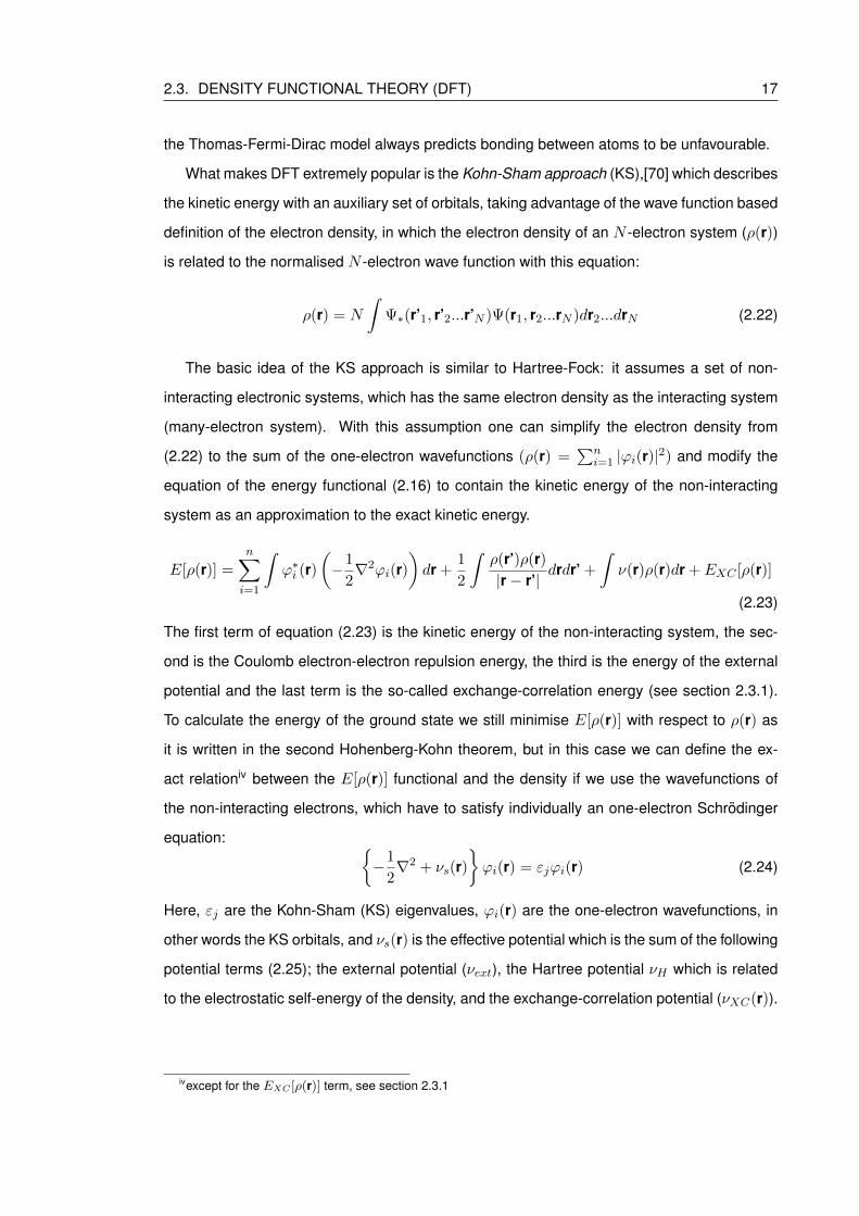
2.3. DENSITY FUNCTIONAL THEORY (DFT) 17
the Thomas-Fermi-Dirac model always predicts bonding between atoms to be unfavourable.
What makes DFT extremely popular is the Kohn-Sham approach (KS),[70] which describes
the kinetic energy with an auxiliary set of orbitals, taking advantage of the wave function based
definition of the electron density, in which the electron density of an N -electron system (ρ(r))
is related to the normalised N -electron wave function with this equation:
ρ(r) = N
∫Ψ∗(r’1, r’2...r’N )Ψ(r1, r2...rN )dr2...drN (2.22)
The basic idea of the KS approach is similar to Hartree-Fock: it assumes a set of non-
interacting electronic systems, which has the same electron density as the interacting system
(many-electron system). With this assumption one can simplify the electron density from
(2.22) to the sum of the one-electron wavefunctions (ρ(r) =∑n
i=1 |ϕi(r)|2) and modify the
equation of the energy functional (2.16) to contain the kinetic energy of the non-interacting
system as an approximation to the exact kinetic energy.
E[ρ(r)] =
n∑i=1
∫ϕ∗i (r)
(−1
2∇2ϕi(r)
)dr +
1
2
∫ρ(r’)ρ(r)|r− r’|
drdr’ +
∫ν(r)ρ(r)dr + EXC [ρ(r)]
(2.23)
The first term of equation (2.23) is the kinetic energy of the non-interacting system, the sec-
ond is the Coulomb electron-electron repulsion energy, the third is the energy of the external
potential and the last term is the so-called exchange-correlation energy (see section 2.3.1).
To calculate the energy of the ground state we still minimise E[ρ(r)] with respect to ρ(r) as
it is written in the second Hohenberg-Kohn theorem, but in this case we can define the ex-
act relationiv between the E[ρ(r)] functional and the density if we use the wavefunctions of
the non-interacting electrons, which have to satisfy individually an one-electron Schrodinger
equation: −1
2∇2 + νs(r)
ϕi(r) = εjϕi(r) (2.24)
Here, εj are the Kohn-Sham (KS) eigenvalues, ϕi(r) are the one-electron wavefunctions, in
other words the KS orbitals, and νs(r) is the effective potential which is the sum of the following
potential terms (2.25); the external potential (νext), the Hartree potential νH which is related
to the electrostatic self-energy of the density, and the exchange-correlation potential (νXC(r)).
ivexcept for the EXC [ρ(r)] term, see section 2.3.1

18 CHAPTER 2. ELECTRONIC STRUCTURE THEORY
νs(r) = νext(r) + νH(r) + νXC(r) (2.25)
Note that the exchange-correlation potential νXC(r), by definition (νXC(r) =δEXCδρ(r)
), comes
from the electron density which is calculated from the solution of the one-electron Schrodin-
ger equation. Therefore, we first have to make a guess for the one-electron wavefunction to
construct an electron density which can be used to create the effective potential and then solve
the eigenvalue problem in (2.24). The density which is calculated from the solution defines a
new potential and this cycle goes on, until there is no change in the output density from one
cycle to the next, i.e. self-consistency is achieved. Finally, the self-consistent electron density
can be used to compute the total energy of the ground state, E0[ρ(r)].
2.3.1 Exchange-Correlation Functionals
The weakness of DFT is the definition of EXC [ρ(r)], the exchange-correlation functional. It
contains everything which is left out of the other terms of the energy: the difference between
the exact kinetic energy and the kinetic energy of the non-interacting system, and the non-
Coulomb part of the electron-electron interaction energy. Generally, the exchange and the
correlation part of the functional are treated separately. Their density dependence cannot be
described exactly but there are several methods to approximate them. We can establish an
order of the different approximations based on the level of chemical accuracy which can be
achieved with them. This hierarchy is sometimes referred to as Jacob’s ladder[71] in DFT.
The simplest approach is the so-called Local Density Approximation (LDA), in which the
exchange part of EXC [ρ(r)] is calculated from the exact exchange energy per particle of a
homogeneous electron gas with a given density.
ELDAX [ρ(r)] = AX
∫ρ(r)4/3dr = AX
∫εx(ρ)dr (2.26)
AX is a constant and εx = ρ(r)4/3 is the exchange energy per particle of the uniform elec-
tron gas. Unfortunately, there is no exact formula for the correlation energy part, therefore
parametrisation is required to define one. For example Vosko, Wilk and Nusair[72] used se-
ries of Quantum Monte Carlo simulations[73] of the homogeneous electron gas to create an
analytic interpolation formula for EC [ρ(r)].
A higher level approach compared to LDA is the Generalised Gradient Approximation
(GGA), in which the description of the inhomogeneity of the electron density is improved with

2.3. DENSITY FUNCTIONAL THEORY (DFT) 19
an extra term in the exchange-correlation functional (2.27).
It has been found that it is difficult to use the gradient of the density function as an extra
variable by itself.[74] Thus a reduced dimensionless gradient (s(r) = |∇ρ(r)|/2kFρ(r)) is cre-
ated to scale the changes in the density and is used to define the exchange energy functional.
EGGAX [ρ(r)] = AX
∫εx(ρ)FX(s)dr (2.27)
AX is a constant, εx(ρ) is still the exchange energy per particle of the homogeneous electron
gas and FX(s) is an enhancement factor which describes the increment of the exchange
energy compared to the LDA value.
A common example of the GGA is the BLYP functional that is made up from an exchange
part developed by Becke (1988) which contains one fitted parameter, and a correlation func-
tional created by Lee, Yang and Parr and parametrised from simple systems.[75, 76] Another
example is the PBE functional which was developed by Perdew, Burke and Ernzerhof in 1996;
there is no fitted parameter in its exchange energy functional.[74].
The next step up Jacob’s ladder is the so-called meta-GGA. Besides the electron density
and its first derivative, meta-GGAs depend on the Laplacian of the density (∇2ρ(r)) or the
kinetic energy density (τ(r) in equation (2.28)) of the occupied Kohn-Sham orbitals (ϕocci (r))
which is also a functional of the density.
τ(r) =1
2
occ∑i
|∇ϕi(r)|2 (2.28)
In this work a meta-GGA functional, called TPSS, was used for the calculations. It is a nonem-
pirical functional that was developed by Tao, Perdew, Staroverov and Scuseria and it contains
the τ(r) functional as an extra variable.[77]
The approaches so far do not consider the self-interaction problem. It occurs in DFT calcu-
lations because the approximations to the exchange-correlation functional do not completely
cancel the Coulomb interaction of the electron with itself, as happens in the case of Hartree-
Fock calculations.(see section 2.2) This type of error can be reduced with the use of hybrid
functionals which have an exchange functional partially built up from a Hartree-Fock expres-
sion.
EXC = (1− a)EDFTX + aEHFX + EDFTC (2.29)
0 < a < 1 is the proportion of the HF exchange part in the functional. One of the most
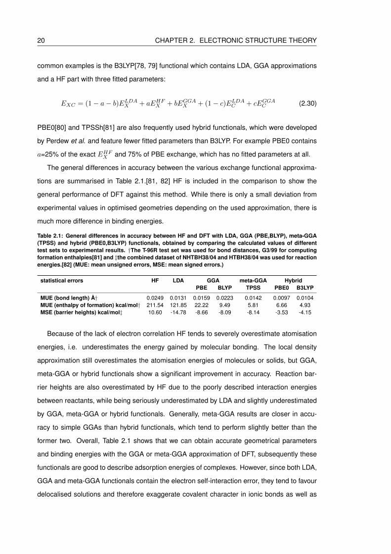
20 CHAPTER 2. ELECTRONIC STRUCTURE THEORY
common examples is the B3LYP[78, 79] functional which contains LDA, GGA approximations
and a HF part with three fitted parameters:
EXC = (1− a− b)ELDAX + aEHFX + bEGGAX + (1− c)ELDAC + cEGGAC (2.30)
PBE0[80] and TPSSh[81] are also frequently used hybrid functionals, which were developed
by Perdew et al. and feature fewer fitted parameters than B3LYP. For example PBE0 contains
a=25% of the exact EHFX and 75% of PBE exchange, which has no fitted parameters at all.
The general differences in accuracy between the various exchange functional approxima-
tions are summarised in Table 2.1.[81, 82] HF is included in the comparison to show the
general performance of DFT against this method. While there is only a small deviation from
experimental values in optimised geometries depending on the used approximation, there is
much more difference in binding energies.
Table 2.1: General differences in accuracy between HF and DFT with LDA, GGA (PBE,BLYP), meta-GGA(TPSS) and hybrid (PBE0,B3LYP) functionals, obtained by comparing the calculated values of differenttest sets to experimental results. †The T-96R test set was used for bond distances, G3/99 for computingformation enthalpies[81] and ‡the combined dataset of NHTBH38/04 and HTBH38/04 was used for reactionenergies.[82] (MUE: mean unsigned errors, MSE: mean signed errors.)
statistical errors HF LDA GGA meta-GGA HybridPBE BLYP TPSS PBE0 B3LYP
MUE (bond length) A† 0.0249 0.0131 0.0159 0.0223 0.0142 0.0097 0.0104MUE (enthalpy of formation) kcal/mol† 211.54 121.85 22.22 9.49 5.81 6.66 4.93MSE (barrier heights) kcal/mol‡ 10.60 -14.78 -8.66 -8.09 -8.14 -3.53 -4.15
Because of the lack of electron correlation HF tends to severely overestimate atomisation
energies, i.e. underestimates the energy gained by molecular bonding. The local density
approximation still overestimates the atomisation energies of molecules or solids, but GGA,
meta-GGA or hybrid functionals show a significant improvement in accuracy. Reaction bar-
rier heights are also overestimated by HF due to the poorly described interaction energies
between reactants, while being seriously underestimated by LDA and slightly underestimated
by GGA, meta-GGA or hybrid functionals. Generally, meta-GGA results are closer in accu-
racy to simple GGAs than hybrid functionals, which tend to perform slightly better than the
former two. Overall, Table 2.1 shows that we can obtain accurate geometrical parameters
and binding energies with the GGA or meta-GGA approximation of DFT, subsequently these
functionals are good to describe adsorption energies of complexes. However, since both LDA,
GGA and meta-GGA functionals contain the electron self-interaction error, they tend to favour
delocalised solutions and therefore exaggerate covalent character in ionic bonds as well as
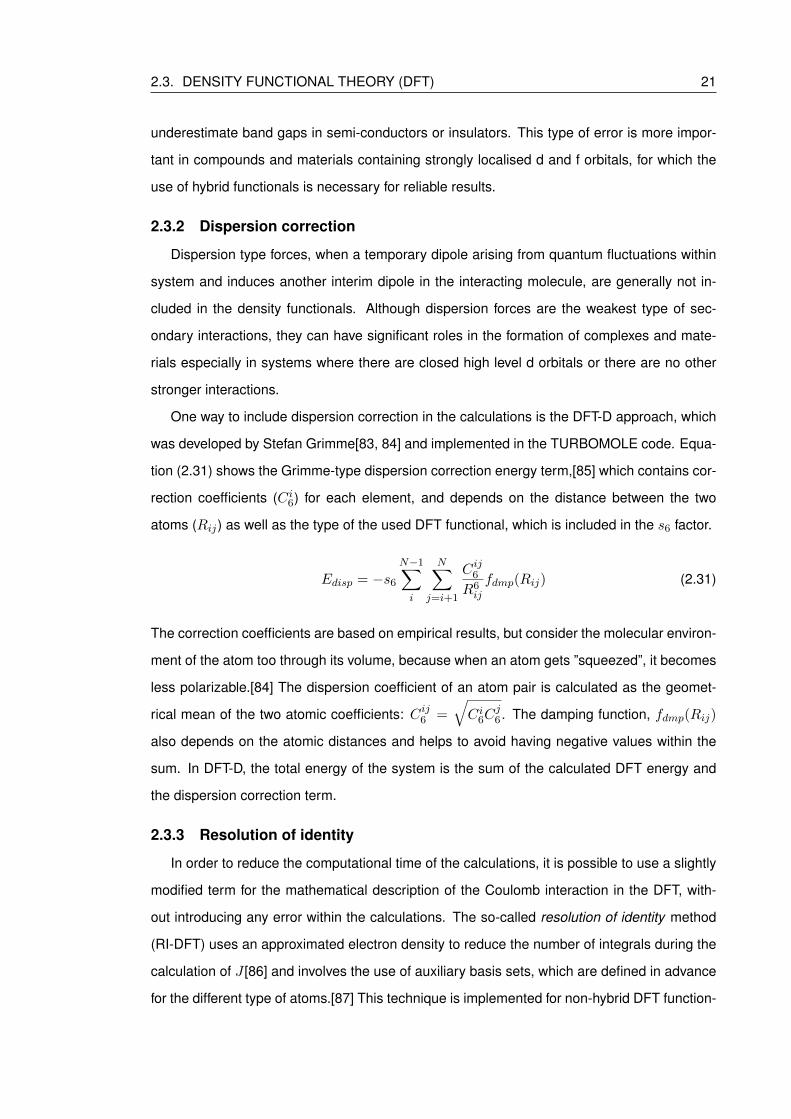
2.3. DENSITY FUNCTIONAL THEORY (DFT) 21
underestimate band gaps in semi-conductors or insulators. This type of error is more impor-
tant in compounds and materials containing strongly localised d and f orbitals, for which the
use of hybrid functionals is necessary for reliable results.
2.3.2 Dispersion correction
Dispersion type forces, when a temporary dipole arising from quantum fluctuations within
system and induces another interim dipole in the interacting molecule, are generally not in-
cluded in the density functionals. Although dispersion forces are the weakest type of sec-
ondary interactions, they can have significant roles in the formation of complexes and mate-
rials especially in systems where there are closed high level d orbitals or there are no other
stronger interactions.
One way to include dispersion correction in the calculations is the DFT-D approach, which
was developed by Stefan Grimme[83, 84] and implemented in the TURBOMOLE code. Equa-
tion (2.31) shows the Grimme-type dispersion correction energy term,[85] which contains cor-
rection coefficients (Ci6) for each element, and depends on the distance between the two
atoms (Rij) as well as the type of the used DFT functional, which is included in the s6 factor.
Edisp = −s6
N−1∑i
N∑j=i+1
Cij6R6ij
fdmp(Rij) (2.31)
The correction coefficients are based on empirical results, but consider the molecular environ-
ment of the atom too through its volume, because when an atom gets ”squeezed”, it becomes
less polarizable.[84] The dispersion coefficient of an atom pair is calculated as the geomet-
rical mean of the two atomic coefficients: Cij6 =√Ci6C
j6 . The damping function, fdmp(Rij)
also depends on the atomic distances and helps to avoid having negative values within the
sum. In DFT-D, the total energy of the system is the sum of the calculated DFT energy and
the dispersion correction term.
2.3.3 Resolution of identity
In order to reduce the computational time of the calculations, it is possible to use a slightly
modified term for the mathematical description of the Coulomb interaction in the DFT, with-
out introducing any error within the calculations. The so-called resolution of identity method
(RI-DFT) uses an approximated electron density to reduce the number of integrals during the
calculation of J [86] and involves the use of auxiliary basis sets, which are defined in advance
for the different type of atoms.[87] This technique is implemented for non-hybrid DFT function-
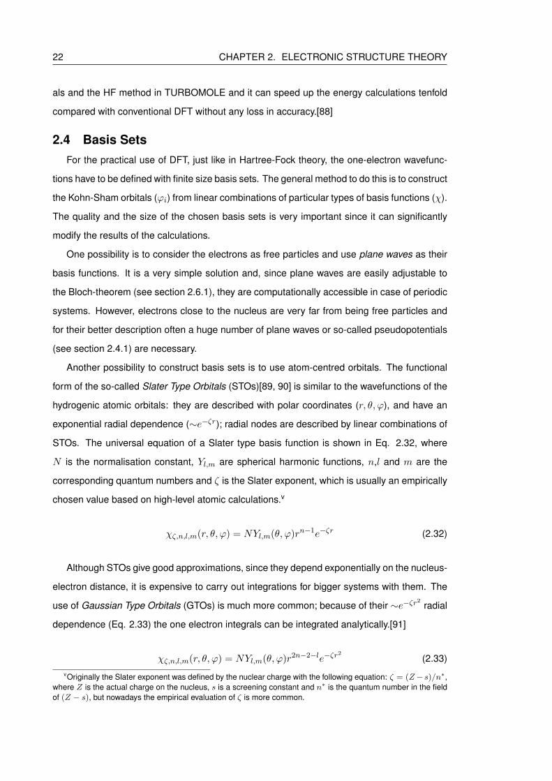
22 CHAPTER 2. ELECTRONIC STRUCTURE THEORY
als and the HF method in TURBOMOLE and it can speed up the energy calculations tenfold
compared with conventional DFT without any loss in accuracy.[88]
2.4 Basis SetsFor the practical use of DFT, just like in Hartree-Fock theory, the one-electron wavefunc-
tions have to be defined with finite size basis sets. The general method to do this is to construct
the Kohn-Sham orbitals (ϕi) from linear combinations of particular types of basis functions (χ).
The quality and the size of the chosen basis sets is very important since it can significantly
modify the results of the calculations.
One possibility is to consider the electrons as free particles and use plane waves as their
basis functions. It is a very simple solution and, since plane waves are easily adjustable to
the Bloch-theorem (see section 2.6.1), they are computationally accessible in case of periodic
systems. However, electrons close to the nucleus are very far from being free particles and
for their better description often a huge number of plane waves or so-called pseudopotentials
(see section 2.4.1) are necessary.
Another possibility to construct basis sets is to use atom-centred orbitals. The functional
form of the so-called Slater Type Orbitals (STOs)[89, 90] is similar to the wavefunctions of the
hydrogenic atomic orbitals: they are described with polar coordinates (r, θ, ϕ), and have an
exponential radial dependence (∼e−ζr); radial nodes are described by linear combinations of
STOs. The universal equation of a Slater type basis function is shown in Eq. 2.32, where
N is the normalisation constant, Yl,m are spherical harmonic functions, n,l and m are the
corresponding quantum numbers and ζ is the Slater exponent, which is usually an empirically
chosen value based on high-level atomic calculations.v
χζ,n,l,m(r, θ, ϕ) = NYl,m(θ, ϕ)rn−1e−ζr (2.32)
Although STOs give good approximations, since they depend exponentially on the nucleus-
electron distance, it is expensive to carry out integrations for bigger systems with them. The
use of Gaussian Type Orbitals (GTOs) is much more common; because of their ∼e−ζr2 radial
dependence (Eq. 2.33) the one electron integrals can be integrated analytically.[91]
χζ,n,l,m(r, θ, ϕ) = NYl,m(θ, ϕ)r2n−2−le−ζr2
(2.33)vOriginally the Slater exponent was defined by the nuclear charge with the following equation: ζ = (Z− s)/n∗,
where Z is the actual charge on the nucleus, s is a screening constant and n∗ is the quantum number in the fieldof (Z − s), but nowadays the empirical evaluation of ζ is more common.
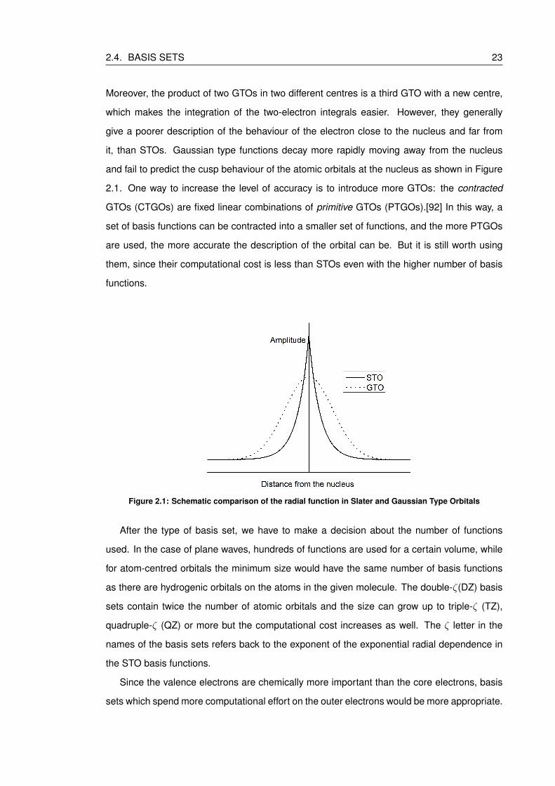
2.4. BASIS SETS 23
Moreover, the product of two GTOs in two different centres is a third GTO with a new centre,
which makes the integration of the two-electron integrals easier. However, they generally
give a poorer description of the behaviour of the electron close to the nucleus and far from
it, than STOs. Gaussian type functions decay more rapidly moving away from the nucleus
and fail to predict the cusp behaviour of the atomic orbitals at the nucleus as shown in Figure
2.1. One way to increase the level of accuracy is to introduce more GTOs: the contracted
GTOs (CTGOs) are fixed linear combinations of primitive GTOs (PTGOs).[92] In this way, a
set of basis functions can be contracted into a smaller set of functions, and the more PTGOs
are used, the more accurate the description of the orbital can be. But it is still worth using
them, since their computational cost is less than STOs even with the higher number of basis
functions.
Figure 2.1: Schematic comparison of the radial function in Slater and Gaussian Type Orbitals
After the type of basis set, we have to make a decision about the number of functions
used. In the case of plane waves, hundreds of functions are used for a certain volume, while
for atom-centred orbitals the minimum size would have the same number of basis functions
as there are hydrogenic orbitals on the atoms in the given molecule. The double-ζ(DZ) basis
sets contain twice the number of atomic orbitals and the size can grow up to triple-ζ (TZ),
quadruple-ζ (QZ) or more but the computational cost increases as well. The ζ letter in the
names of the basis sets refers back to the exponent of the exponential radial dependence in
the STO basis functions.
Since the valence electrons are chemically more important than the core electrons, basis
sets which spend more computational effort on the outer electrons would be more appropriate.
24 CHAPTER 2. ELECTRONIC STRUCTURE THEORY
Split valence basis sets separate the core and valence orbitals in the atoms, and while the
core orbitals are a contraction of a number of PGTOs, the valence orbitals split into more
functions. For example, in the 3-21G basis set which was developed by Pople et al.,[93] the
core orbitals are described at single-zeta quality with a linear combination of three PGTOs,
while the valence orbitals have double-zeta basis sets, which contain one CGTO formed the
linear combination of two PGTOs and a single PGTO as the second function.
In the basis set family which was used in the present calculations (def2-SVP, def2-TZVP
and def2-QZVP from R. Ahlrichs[94]), the core orbitals are represented by one CGTO, while
the valence orbitals are described at the double-, triple- and quadruple-ζ level (SV, TZV and
QZV respectively) and with a set of polarisation functions (P) which is a set of basis functions
with a higher angular momentum than the occupied valence orbitals. They are used to im-
prove the description of non-spherical electron distributions with their higher angular nodality,
therefore allowing the definition of possible anisotropic interactions within the chemical bonds.
2.4.1 Effective Core Potentials (ECPs)
The core electrons of heavier elements do not play a significant role in the formation of
molecular bonds but plenty of primitive GTOs are needed to expand them properly (to de-
scribe the electron-electron repulsion with the valence orbitals). Moreover, in the case of the
elements from the lower part of the periodic table, relativistic effects cannot be neglected.
With the use of the so-called Effective Core Potentials[95] one can significantly reduce the
computational cost and take into account part of the relativistic effects as well.
In the ECPs, the core orbitals are replaced with a pseudopotential function constructed
to model the chosen core electrons instead of a large number of basis functions. First, an
accurate wavefunction is calculated with the use of a high-level all-electron basis set. Then
the valence orbitals are replaced with nodeless functions, in a way that the created pseudo-
orbitals of the valence electrons do not have core nodes, but still describe the nodal structure
with the new core function correctly. The next step is to exchange the core electrons for a
parametrised potential expanded as a set of analytical functions, and fit the parameters such
that the Schrodinger equation produces pseudo-orbitals matching all-electron valence orbitals.
If GTOs are used for the valence orbitals, the ECP is a Gaussian type function too. In this
case, the quality of the ECP depends on the number of electron orbitals chosen to be repre-
sented by the new core function. Evidently, having less electrons merged into the ECP and
more on valence type orbitals increases the accuracy, while also increasing the computational
2.5. SOLVENT MODELS 25
cost. In our case, the investigated systems have an ECP and the associated valence basis set
to describe the core electrons in the 1s-3d orbitals of the Sr atom, similarly, ECPs are used
for calculations involving the Rb (1s-3d orbitals), and Ba, Cs (1s-4d orbitals) atoms in section
4.5.1.[96, 97]
2.4.2 Basis Set Superposition Error (BSSE)
The use of finite size atomic centred basis sets introduces an error which is especially
important in the case of weak interactions between molecules. The problem lies in the fact
that in a complex formed by an interaction between two molecules, the energy of the com-
plex is calculated with a basis set composed from the basis sets of both molecules. It means
that the molecules in the complex are treated with a more complete basis set than the in-
dividual ones. Therefore the energy of the complex is artificially lower and the strength of
the interaction is overestimated. This problem is the so-called Basis Set Superposition Error
(BSSE) and one way to avoid it is to increase the size of the basis set, but this significantly
increases the computational cost. Thus the most common way to compensate for the BSSE
is to use an approximation, the Counterpoise Correction (CP),[98] to evaluate the error. In this
method we use ’ghost functions’ which are the basis sets of one molecule located at the cor-
responding nuclear position but without the nuclei or electrons, to improve the basis set of the
other molecule. These modified basis sets are used to calculate the energy of the individual
molecules (E(A)∗ab,E(B)∗ab). In addition, we calculate the energy of the individual molecules
with the same geometries that they have in the complex but with their own basis sets only
(E(A)∗a,E(B)∗b ). The value of the error can be calculated from these results according to the
following equation:
∆ECP = E(A)∗ab + E(B)∗ab − E(A)∗a − E(B)∗b (2.34)
The counterpoise correction was used here to compensate for the BSSE error in the studied
adsorption reactions, since the basis set of the isolated ions or systems is significantly smaller
than the overall basis set of the adsorbed complexes with the surface.
2.5 Solvent Models
If the studied systems are solvated, the effects of the solvent can significantly modify their
properties compared to the results in vacuum. There are two ways to take into account the
solvation; one is to describe explicitly the solvent molecules and the other is to consider the
26 CHAPTER 2. ELECTRONIC STRUCTURE THEORY
solvent implicitly, as a continuous medium. Expanding the system with individual solvent
molecules is necessary if one would like to include the short-range, specific, interactions be-
tween the solvent and the molecule, such as the effects of hydrogen bonds, van der Waals
interaction etc. However, modelling the first solvation shell will not describe the long-range
interactions: the polarisation or the dipole orientation effect of the solvation. In most cases
the solute is ionic or it is a neutral molecule with a dipole moment, which arises due to the
non-homogeneous charge distribution within the molecule. The solute polarizes the polar-
isable medium (described with a relative permittivity, εr) and modifies the orientation of its
electric multipole moments, which then acts back on the solvated system. If the structure
of the molecule (solute or solvent) is very symmetric or apolar, the dipole moment or the
permittivity is very small and these non-specific interactions have no significant effect on the
system. But in any other cases, the long-range interactions can modify the orientation of the
surrounding solvent molecules, as well as the optimal geometry and the free energy of the
solvated molecule.[99] Since including enough solvent molecule explicitly to model these non-
specific effects is practically impossible with ab-initio quantum chemical methods, we have to
use QM/MM methods or Continuum Solvent Models to efficiently consider their contribution.
[100]
2.5.1 Continuum Solvent Models (CSM)
In the CSM methods, the solvent is treated as a homogeneous polarisable medium with a
dielectric constant (which is the relative permittivity of the solvent, εr), while the molecule is
surrounded with a suitably shaped cavity in the medium.[99] The solvation free energy can be
described with the following terms in this system:
∆Gsolv = ∆Gcavity + ∆Gdispersion + ∆Gelectrostatic (2.35)
The term related to the formation of the cavity (∆Gcavity) is positive, since the loss of the
solvent-solvent interactions has a destabilising effect. The newly formed dispersion interac-
tions between the solute and the solvent (∆Gdispersion) as well as the electrostatic interactions
in term ∆Gelectrostatic give a negative contribution to the energy of the solvated system.
One key question of CSM methods is the definition of the cavity, since ∆Gcavity and
∆Gdispersion are often assumed to be directly proportional to the the total surface area and
the solution of ∆Gelectrostatic is also related to the cavity. Although employing spherical or
ellipsoidal shaped cavities would allow the analytical solution of the electrostatic term, gen-

2.5. SOLVENT MODELS 27
erally a level of molecular surface description is needed for acceptable results compared to
experimental data. One way to define molecular shaped holes is to consider every atom in
the solute as a sphere with a radius of the atomic radius times the van der Waals radius of
the atom. The atom-centred spheres overlap with each other and create the van der Waals
(vdW) surface, shown in Figure 2.2. Most of the solvent models operate with vdW surfaces
because it is computationally cheaper and still very similar to other more complicated surface
descriptions, such as the so-called solvent accessible surface (SAS) traced out by the centre
of solvent sphere rolling over the vdW surface or the molecular surface is the lower envelope
generated by the rolling solvent.[101] They were both created because the vdW surface may
contain small parts, where the solvent molecules are too big to enter. A different way to define
a cavity is to use a surface related to a given electron density value. This approach is less
common because we need the whole wave function for the density based surface construc-
tion.
Figure 2.2: Different definitions of the cavity surface[102]
The electrostatic stabilisation arises because the charge distribution of the molecule (ρM )
induces a charge moment in the solvent which acts back and polarises the molecule, chang-
ing its charge distribution. One can easily see that calculating this term is a self-consistent
process, which requires an iterative solution.[101, 103] When the molecule is surrounded with
a polarisible medium, the electrostatic potential term within the quantum mechanical frame-
work (V ) is extended with a solvent reaction potential (VR), generated by the polarization of
the dielectric medium:V = Vρ + VR (2.36)
Where Vρ is the electrostatic potential related to the overall charge distribution including the
electronic and nuclear components. The most common way to evaluate the reaction potential
is to integrate the partial surface charges (σ(s)) screening the cavity surface (Eq. 2.37),
where s is the position variable on the cavity surface. However, we need the total electrostatic
28 CHAPTER 2. ELECTRONIC STRUCTURE THEORY
potential within the cavity to calculate σ(s), using a simplified form of the classical Poisson
equation, shown in Eq. 2.38, where F is the derivative of V perpendicular to the surface and
εr is the dielectric constant of the solvent.
VR =
∫σ(s)
|r− s|d2s (2.37)
σ(s) =εr − 1
4πεrF (2.38)
Similarly to the previously shown self-consistent field process 2.2, we first have to make a
guess for the charge density (ρM ) to construct the electrostatic potential which can be used
to calculate the surface charge on the cavity and the reaction potential. Including VR modifies
the total electrostatic potential, which gives a new surface charge and this cycle goes on, until
there is no significant change in the output potential from one cycle to the next. The actual
∆Gelectrostatic term is calculated based on the dipole moment and polarizability, evaluated
from the final charge distribution.
Although CSMs are convenient to implement and use in QM codes, they have their limi-
tations, since εr is the only parameter characterising the solvent. For example solvents with
very similar dielectric constant will behave the same using this model while they might differ
significantly in reality due to possible hydrogen bonds or differences in planarity. Besides,
εr is treated as a constant in the continuum models, while it can depend for instance on the
distance from the solute or the speed of the reaction.
In chapter 3 the so-called conductor-like screening model (COSMO)[104, 105] is used, as
implemented in the TURBOMOLE code. It employs molecular shape cavities based on the van
der Waals radii of the atoms in the molecule. The cavity is defined in the beginning of every
SCF cycle and the dispersion free energy terms are parametrised based on the surface area
of the cavity. The electrostatic contribution is defined from the electrostatic potential by partial
atomic charges which are calculated with a self-consistent reaction field model, assuming
an infinite dielectric constant εr = ∞, i.e. conductor-like behaviour for every solvent. This
assumption results in zero potential on the cavity surface (V = Vρ+VR = 0), and significantly
simplifies the use of Eq. 2.38, which instead of the normal component of V (F), only depends
on a local value. However, the final surface charge obtained with an infinite permittivity (σ∗(s))
has to be corrected with an empirical scaling function (f(εr)) to recover the effect of the finite
value of the εr (Eg. (2.39)).[101] The scaling factor is determined by comparing the unscaled
COSMO results to known electrostatic solute-solvent energies and the following formula is
2.6. PERIODIC ELECTRONIC STRUCTURE METHODS 29
employed (where k is a small value, 0.5 in TURBOMOLE[106]):
σ(s) = f(εr)σ∗(s) =
εr − 1
εr + k(2.39)
To avoid any electron density ”leaking out” from the molecular cavity for example due to
diffuse basis sets on atoms close to the cavity surface, TURBOMOLE employs a so-called
outlying charge correction (OC) during the COSMO calculations. At the end of the converged
SCF a new outer surface with increased radii is constructed to evaluate the OC correction term
for the dielectric energy and added to the value calculated with original cavity surface.[107]
As it was stated before, the cavity is defined at the beginning of every SCF cycle and
checked for outlying charges at the end of SCF convergence. In case of vibrational frequency
calculations a problem may arises due to the different time-scale of the molecular vibrations
and the solvent re-orientation (the former is much faster than the latter). Since the normal
modes are obtained by a series of single point calculations in which the individual atoms are
slightly displaced to study their motion (see section 2.7.2), the cavity is defined differently for
each distorted geometry and electrostatic energy difference arising from the electron density
difference is evaluated.[106]
The COSMO solvent model plays and important role this thesis. First, in chapter 3 it
is shown applying a constant dielectric continuum has a significant effect on the optimised
geometries and its use is necessary to obtain realistic energies for the Sr2+ complexes. Sub-
sequently, in chapter 5 a modified COSMO correction term is employed to allow the energetic
comparison of the adsorbed complexes on the hydrated brucite surfaces with structures in the
bulk solvent.
2.6 Periodic Electronic Structure Methods
Crystalline materials are rather different from isolated molecular structures: they are built
up by a large number of atoms and/or molecules, which form a well defined symmetrical
structure with significant intermolecular interactions between the structural units. Every crystal
material has some kind of translational invariance, i.e. the atom in position r is equivalent to
the atom in r’:
r’ = r +3∑j=1
Njaj (2.40)
Where aj are the basis vectors in the three spatial direction (j = 1, 2, 3 as a, b, c), Nj are the
number of times that the translation was repeated in j directions.
30 CHAPTER 2. ELECTRONIC STRUCTURE THEORY
Modelling solids heavily relies on the fact that there is a proven relation between the spatial
symmetry of the systems and the physical property of the material. Based on the above shown
translational invariance, one can apply periodic boundary conditions[108] (PBCs) to reduce
the practically infinite size of the systems to finite size units while still aiming to calculate
properties related to the whole material.
I briefly summarise the basics of two methods developed to model solid materials, both
of which have their advantages and disadvantages depending on the interest of the solid
phase study. Periodic density functional theory is the most common approach to investigate
crystalline materials and their properties, while the periodic electrostatic embedded cluster
method was specifically developed to study isolated defects or surface reactions of solid ma-
terials.
2.6.1 Periodic Density Functional Theory
For bulk studies, any effects related to the surfaces can be neglected to consider the real
crystal as infinite and translation invariant.[54, 109] Assuming independent electrons moving
in the periodic potential field of the solid material, described by a periodic function having the
same periodicity as the crystal (V (r’) = V (r)), one can apply the Schrodinger equation to
describe the energy states of the studied solid. Since the Hamiltonian operator, containing V ,
has to be translation invariant too, we can write down the following equalities for the SE:
Tg
(H(r)Ψ(r)
)= H(r)TgΨ(r) = H(r)Ψ(r’) (2.41)
Tg is the translation operator, which leaves the Hamiltonian invariant, i.e. if Ψ(r) is the eigen-
function of the Hamiltonian, TgΨ(r) = Ψ(r’) is an eigenfunction with the same energy too.
The Bloch theorem[110] defines the relation between the periodic Hamiltonian and the
wavefunction by stating that: wavefunctions, which are the solutions of the periodic SE eq. in
equivalent positions in the lattice of different unit cells, only differ by a k related phase factor,
eikg shown in (2.42), where k is the wave vector. Any Ψ(r) obeying to this symmetry rule is a
Bloch function (BF, also known as Bloch wave) Φnk(r), and can be written as a product of a
plane wave and a periodic function with the same periodicity as the crystal (2.43). Note that,
not k nor the periodic function (unk), only the wavefunction determines uniquely the quantum
state of the electron because, there are more then one periodic functions for the same k
differing by their n band index; while for a given n Φnk varies continuously with k, creating a
continuous energy band.
2.6. PERIODIC ELECTRONIC STRUCTURE METHODS 31
Φnk(r’) = Φnk(r + g) = eikgΦnk(r) (2.42)
Φnk(r) = eikrunk(r) (2.43)
One can contract the problem originally spanned over the infinite crystal to a finite sized
N = N1xN2xN3 cell, by combining the Bloch theorem with the periodic boundary conditions
(Eq. (2.40)) and define the allowed k vectors such that the phase vector equals to one for any
integer α and every j = 1, 2, 3:
Φnk(r + αNjaj) = eiαNjkajΦnk(r) where eiαNjkaj = 1 (2.44)
The k points which satisfy this requirement are defined by the basis vectors of the reciprocal
lattice (bj) and the mj integer: k =∑3
j=1
mj
Njbj . There are N = N1xN2xN3 number of
k points allowed in every reciprocal lattice cell and when N is a huge number, k is practi-
cally a continuous variable. The fact that the wave vector is defined in the reciprocal space,
makes every wavefunction translated by any reciprocal lattice vector (K =∑3
j=1mjbj) equal:
Φn(k) = Φn(k + K), and allows us to restrict the analysis of the Bloch functions entirely to the
first Brillouin zone (BZ)vi.
Operating with the Bloch functions in reciprocal space and using a finite number of them as
basis functions simplifies the evaluation of the expectation value of the Hamiltonian. If all the
integrals in the solution of the SE equations are periodic functions with the same periodicity
of the latticevii and the Bloch functions are expanded with a linear combination of plane waves
(Φnk =∑
K ck,Kei(k+K)r), the eigenvalue of the SE equation can be evaluated by summing up
integrals only involving plane waves:
⟨Φn,k’(r)|Hk,k’(r)|Φn,k(r)
⟩=∑
K
cK
∑K’
cK’
∫ei(k’+K’)rH(r)ei(k+K)rdr (2.45)
Due to the orthogonality of the plane waves, these integrals are always zero except if the wave
vectors of the functions are the same (k = k′).
Therefore, the Hamiltonian can be defined as a block diagonal matrix, containing nxn
viThe first Brillouin zone is basically the Wigner-Seitz type primitive cell of the crystal in reciprocal space; itsdefined by a collection of points which are closer to the origin of a given reciprocal lattice than any other reciprocallattice points.
viiIt was shown earlier that the potential energy function is periodic and the kinetic energy contains the secondderivatives of unk, therefore it has the same periodicity too.
32 CHAPTER 2. ELECTRONIC STRUCTURE THEORY
blocks if there are n Bloch functions in the basis set. Each block is related to an individual k
vector in the reciprocal unit cell, and can be calculated independently from the other blocks.
One can calculate the total energy of the unit cell by solving SE equations for the first Brillouin
zone of the periodic system at a finite number of k points sampling the Hamiltonian matrix
(2.46), keeping in mind that the same number of k points applied for a bigger normal cell as
for a smaller one, will mean a finer sampling in the reciprocal space.
HΨnk(r) = EnkΨnk(r) (2.46)
Similarly to the previously mentioned HF or DFT theories, the practical solution of the one-
electron SE or KS equations is an iterative process in the solid state calculations involving the
use of trial basis functions. In the CRYSTAL code the Bloch functions are constructed from
the linear combination of atomic orbitals, which are usually defined by contracted GTOs[111]
(see section 2.4). Since the Bloch waves have to be periodic with the same periodicity of the
crystal, the AOs are chosen in the unit cell like χµ(r−rµ), where rµ is the origin of the µ orbital
in the first cell, and repeated in the other cells of the crystal to form the µth BF:
Φµ,k(r) =1√N
∑g
ei(kg)rχgµ(r− rµ) (2.47)
The key step of the iteration process in periodic systems that to define the Bloch functions for
the chosen k points in the Hamiltonian matrix, first its components (the one- and two-electron
integrals) have to be defined in real space with the use of the basis functions and then Fourier
transformed from real space to reciprocal space. Once the one-electron SE or KS equations
are solved for each sampling k points in the first BZ and the electron density is evaluated,
it has to be inverse Fourier transformed to real space again to repeat the evaluation of the
integrals until self-consistency achieved.
2.6.2 Periodic Electrostatic Embedded Cluster Method (PEECM)
The primary application of the Periodic Electrostatic Embedded Cluster Method (PEECM)
is to calculate the structure and the properties of isolated defects in ionic crystals or on their
surfaces. With the electrostatic embedding of a finite quantum chemical (QM) region in a
periodic infinite array of point charges (PCs), it is possible to treat the localised defect in the
crystal on the level of any standard ab initio method with a modest computational cost. In
contrast to the PEECM, in periodic DFT calculations the defect concentration is often higher

2.6. PERIODIC ELECTRONIC STRUCTURE METHODS 33
and to avoid false interactions between the defects large supercells are necessary which
significantly increasing the computational cost.[56]
In this method, we divide the entire system to two main parts: an inner cluster and an outer
part. A schematic representation of the subdivisions in the system is shown in Figure 2.3. The
innermost part of the cluster is the local region which contains the defect, not repeated in any
dimension and is treated quantum chemically. There is an isolating shell in the cluster around
the QM region in which the cations are replaced by effective core potentials (ECPs, 2.4.1) or
natural PCs to prevent the artificial polarisation of the electron density in the innermost part
by the nearby point charges.[112] Surrounding the defect is the outer part which is described
as infinite periodic array of PCs.
Figure 2.3: Schematic representation of the different regions in PEECM calculations in the x direction
An electrostatic potential arises in the QM region from the PC field environment which can
be taken into account as an additional energy (Jemb) term in the total energy of the QM region:
Jemb =
∞∑L∈O
N∈UC∑k
(∑µν
Dµνqk
∫µ(r)ν(r)|r− Rk + L|
dr +∑a
qkZa|Ra − Rk + L|
)(2.48)
Jemb contains two terms, one describes the Coulomb interactions between the electrons of
the QM region and the PCs, while the other contains the interactions between the nuclei of
the inner cluster and the PCs. L is a direct lattice vector in the outer part O. UC is the unit
cell and k is the index of an ionic PC, qk at the position Rk − L. µ and ν are Gaussian basis
functions, Dµν is an element of the density matrix, and Za is the nuclear charge at position Ra
in the cluster. Summing over L and k includes the images of all the PCs except the ones in
34 CHAPTER 2. ELECTRONIC STRUCTURE THEORY
the inner cluster.
A difficulty of the PEECM is calculating Jemb for an infinitely large array of PCs, since a
direct sum of all the Coulomb interactions is impossible. A usual approach often applied by
other QM/MM methods is to evaluate the electrostatic energies in the PC field using Ewald
summation.[113, 114] In this method the outer region is divided to two more parts: a near field
part (NF) where the Coulomb interactions are summed up directly in real space, and a far field
part (FF) in which the summation is made in Fourier space.
PEECM uses another approach called the Periodic Fast Multipole Method (PFMM)[115]
which also divides the outer region to NF and FF, but employs multipole expansions for the
FF interactions besides the analytical integration of the Coulomb interactions in the NF. The
size of the near field region is usually given by the well-separateness criterion[115] defined
by the size of the PC unit cell and a separateness constant; which is for instance 3.0 by
default in the TURBOMOLE code. In general, the NF region has to be big enough to allow
a rapid convergence for the multipole approximations in the far field. Using PFMM avoids
having to convert integrations to reciprocal space and back, therefore it is less demanding
computationally than the Ewald summation. First, the basis functions, the nuclear charges
and the PCs are all evaluated by multipole moments of solid harmonics. Then the computed
PC equivalents are expanded as Taylor expansions around the center of the system, using
the periodicity of the unit cell. And finally, the far field components of the electrostatic potential
are calculated using the defined multiple expansions for each term.
PFMM seriously speeds up the calculation of the additional electrostatic potential arising
from the PCs, as a result, PEECM simulations in TURBOMOLE run in a similar time scale than
a standard molecular DFT calculation, only requiring a small fraction of the total computational
cost of a DFT optimisation.[56] This advantage of the PEECM calculations compared to other
approaches played an important role in choosing this particular method to simulate the brucite
surface. The optimisation of the brucite (0001) model in TURBOMOLE and its validation is the
basis of chapter 4, in which we use the PEECM model of brucite to examine the adsorption of
single solvated ions on a surface, a situation which can be compared with an isolated defect.
2.7 Calculations In Practice
Quantum chemical calculations are most often used for structural optimisation of chemical
systems or calculating their energy derived properties, as thermodynamic properties, forces
and electric moments etc. The basic principles of geometry optimisation and vibrational fre-
2.7. CALCULATIONS IN PRACTICE 35
quency calculations are summarised within the sections 2.7.1 and 2.7.2. Besides, the results
of electronic structure calculations, such as the optimised electron density function and molec-
ular orbitals can be used to further investigate the molecular and atomic properties within the
systems. Some of the electronic structure analysis methods are detailed in section 2.7.3.
The general steps of a quantum chemical calculation for obtaining the optimised geometry
are the following: First, we have to create a geometry input, usually in the form of Cartesian or
internal coordinates. Then, based on the Born-Oppenheimer approximation we optimise the
electronic structure separately for the given nuclear coordinates by calculating the total energy
of the system with a self-consistent iterative method. Taking the first and second derivative
of the obtained energy with respect to the atomic displacements helps us to define a new
set of coordinates and the SCF calculation has to be repeated for the new energy, continuing
this process until self-consistency achieved for the geometry optimisation too. The optimised
structure, together with its total energy and the electron density function related to the ob-
tained atomic coordinates can be the input of further calculations investigating properties of
the system.
2.7.1 Geometry Optimisation
During the geometry optimisation we are seeking specific points on the potential energy
surface, which are stationary points of the energy function, i.e. their first derivative (the gradi-
ent) is zero and their second derivatives are all positive or contain one or more negative eigen-
values, depending on the nature of the characteristic point: the local minima (2nd derivatives
are all positive) correspond to stable structures such as reactants, products or intermediates,
while stationary points with only one negative 2nd derivative are related to transition states,
i.e. to the lowest saddle point between two minima.
Most of the geometry optimisation methods used in this study follow an iterative proce-
dure, during which the atomic coordinates are changed step by step towards the optimum,
while the gradient vector is calculated analytically for each step and the matrix containing the
second derivatives (Hessian matrix) is approximated. The optimisation is finished when the
following criteria are all satisfied: the energy change between two optimisation steps is below
a certain value and both the maximum displacement and the maximum gradient elements
with the RMS of them are below a given value too. Most of the quantum chemical codes,
such as TURBOMOLE, use a quasi-Newton-Rapshon method [116] to determine the atomic
displacement of the steps, in which a restricted second order Taylor expansion of the energy

36 CHAPTER 2. ELECTRONIC STRUCTURE THEORY
function is used to calculate the next step.[106] Controlling the step size and its direction is
important to avoid regions where the quasi-NR approximation is not valid and to make sure
that every step takes the energy closer to the minimum. TURBOMOLE uses a shift parame-
ter to make the step size equal to the trust radius, which is known as the quadratic method.
Since minimising the whole Hessian matrix and diagonalising it is the computationally most
demanding part of the optimisation process, so-called updating schemes are employed to re-
duce the cost. In TURBOMOLE, the first guess of the Hessian is the scaled unity matrix if no
other initial approximation is available, and it is improved rapidly with each step by considering
the calculated gradient for that direction. With the use of the BFGS[117] updating algorithm,
the Hessian is guaranteed to be always positive which can lead to the local minimum in fewer
steps.viii
2.7.2 Frequency Calculation
Generally in electronic structure studies the ground state energy is calculated at 0K in a
hypothetical, motionless state, while in reality the studied systems are at a finite temperature
where they have translational, rotational and vibrational motions. For some cases it is pos-
sible to take these into account in the energy by calculating thermodynamic corrections for
the investigated systems.ix In this way, the total energy is calculated as a sum of the zero
point energy, and the translational, rotational and vibrational energy contribution at the given
temperature. The energy related to the first two types of motion usually equals 2/3kBT per
molecule while the vibrational energy has to be calculated from its normal modes. There are
3N − 6 vibrational modes in a non-linear molecule and their frequencies and the displace-
ments of the individual atoms can be evaluated from the Hessian matrix once a single point
energy was calculated for the given motion. After making the elements of the Hessian ma-
trix mass-dependent and diagonalising it, the vibrational frequencies are obtained from its
eigenvalues, assuming that the energy surface is harmonic close to the energy minimum.
Depending on the size of the studied systems, the Hessian matrix may be calculated ana-
lytically or numerically; the latter is not exact and differences of ±10 cm−1 in the frequencies
can appear. These deviations are more apparent for the first six eigenvalues, which belong to
the translational and rotational modesx and should be zero for a fully optimised structure.
viiiBFGS stands for the Broyden-Fletcher-Goldfarb-Shanno method. For transition state optimisation anotheralgorithm should be used to allow negative eigenvalues.[117]
ixThermodynamic corrections are not applicable for systems with frozen coordinates.xThis is true when Cartesian coordinates are used for the structure.
2.7. CALCULATIONS IN PRACTICE 37
2.7.3 Electronic Structure Analysis
Referring back to the first Hohenberg-Kohn theorem (2.3), the electron density of the
ground state uniquely defines the external potential, and vice versa, the external potential
arising from the nuclei uniquely determines the distribution of the electrons. This is a powerful
statement, which means that atomic and molecular properties can be derived from the function
of the electron density (ρ(r)). Among the several existing analysing techniques, this summary
only concentrates on the methods which I applied during my PhD: the quantum theory of
atoms in molecules (2.7.3.1), natural population analysis (2.7.3.2) and the 3D distribution of
the electron density difference (2.7.3.3).
2.7.3.1 Quantum Theory of Atoms in Molecules (QTAIM)
In the QTAIM, developed by Richard F. W. Bader,[118, 119] the electron density is analysed
in terms of its topology to describe atoms and their properties in molecules.xi
The general concept of this theory is to divide the molecular volume into so-called atomic
basins, via the derivation of the electron density function with respect to its three spatial coor-
dinates. The gradient of ρ(r) is zero at the critical points (2.49), which can be classified into
four categories based on the number of negative eigenvalues of the Hessian matrix of the
electron density (A in Eq. (2.50)).[118, 120]
∇ρ(r) =
0 if r = rC or∞
6= 0
(2.49)
A(rC) =
∂ρ∂x2
∂2ρ∂x∂y
∂2ρ∂x∂z
∂2ρ∂y∂x
∂ρ∂y2
∂2ρ∂y∂z
∂2ρ∂z∂x
∂2ρ∂z∂y
∂ρ∂z2
(2.50)
The general notation of the different type of CPs is (m,n) where m is the number of non-
zero eigenvalues of the Hessian matrix at the critical points and n is the difference between
the number of positive and negative eigenvalues:
Critical points with three negative eigenvalues (3,-3), are local maxima and represent the
nuclei, which attract the electrons with their positive charges, thus ∇ρ(r) points towards the
strongest local nucleus at every point in space and goes to zero infinitely far from it. However,
there are spacial trajectories of the maximum gradient, which terminate in other nuclei andxiMolecules are understood in an extended meaning, i.e., it also contains molecular or ionic crystals, weakly
bonded molecular complexes etc.
38 CHAPTER 2. ELECTRONIC STRUCTURE THEORY
known as bond paths. Each atomic basin is associated with one nucleus and separated from
the neighbouring basins by a two-dimensional surface, known as zero-flux surface, which
is not intersected by the gradient vectors in any point. If a particular atomic property can be
expressed in terms of a corresponding property density in space, we can integrate that term in
an atomic basin to calculate that property, such as the atomic charge or the dipole, quadrupole
moment of the atom etc. Consequently, molecular properties can be evaluated as a sum of
the obtained atomic contributions.
Critical points with two negative and one positive eigenvalues (3, -1), are called Bond
Critical Points (BCPs). They are situated on bond paths and are local minima along the
direction of the nuclei and maxima in the plane perpendicular to this axis.
Ring Critical Points (RCPs) have one negative eigenvalue (3, 1), and they are most likely
positioned close to the middle of the atomic rings in molecules.
Cage Critical Points (CCPs) have no negative eigenvalues (3, 3), in the Hessian matrix.
An other important parameter derived from the second derivatives is the Laplacian of the
electron density [∇2ρ(r)], which is the trace of the diagonalised Hessian matrix, i.e. the sum
of its eigenvalues. The Laplacian at the BCPs describes the nature of the bond: if the electron
charge is locally depleted, the sign of ∇2ρ(r) is positive, which is most likely occur in closed-
shell interactions such as hydrogen-bonds; while if the electron charge is increased within the
intermolecular region, the Laplacian is negative, as happens for covalent bonds.[121]
The strength and nature of the chemical bonds is also reflected in the electron density at
the BCPs (ρb). In general, it is greater than 0.2 a.u. for covalent bonds and smaller than 0.10
a.u. for weaker, closed shell interactions. There are several examples in the literature where
strong correlation was found between QTAIM properties such as ρb values or the[∇2ρ(r)] and
other properties e.g. bond lengths[122–125] or bonding energies[121, 126–128].
In a typical QTAIM calculation, first a wavefunction is generated from an electronic struc-
ture calculation. The hereby used file format, .wfn, holds the atomic coordinates along with
the orbital energies, occupancy numbers and the used Gaussian type functions and their ex-
pansion coefficients. Since this file format may not be directly available in the used quantum
chemistry code, the use of a converter program, such as molden2aim[129], can be necessary.
The electron density is obtained from the wavefunction and used point-by-point for the topo-
logical analysis. After the CPs and bond paths are calculated, the atomic partitions can be
defined along the zero-flux surfaces in the molecular space and the required atomic properties
can be evaluated via integration over the atomic basins. The QTAIM theory is implemented in

2.7. CALCULATIONS IN PRACTICE 39
several codes, such as AIMALL,[130] which was developed by T. A. Keith. In order to obtain
meaningful QTAIM analysis, basis sets which are capable to accurately describe the bonding
regions in molecules have to be used to calculate the electron density, i.e. basis sets contain-
ing polarization functions are necessary. If effective core potentials (ECPs, 2.4.1) are used
for any atoms in the molecule (such as Sr), only certain parameters, which depend only on
the spatial coordinates like the electron density, can be calculated via QTAIM and at least one
sub-valence shell has to be included explicitly to be able calculate the integrated properties.
2.7.3.2 Natural Population Analysis (NPA)
Natural Population Analysis (NPA) was first introduced by Weinhold et al.[131] to use the
concept of natural atomic orbitals (NAOs) for calculating atomic charges (natural charges) and
for deriving molecular bonds between atoms. The basic idea of NPA is to construct the atomic
orbitals in the molecular environment based on the one-electron density matrix, similarly to the
natural orbitals (NOs), which are the molecular orbitals of maximal occupancy for the given
molecular wave function derived from the molecular first order density matrix (Γ(1|1′)).[132,
133]
NAOs are the atomic orbitals of maximal occupancy for the same molecular wave function
as NOs, but obtained from the atomic angular symmetry segments of the original density
matrix, i.e. Γ is defined in terms of matrix block of basis functions belonging to the atomic
centers (e.g. ΓAA) as it is shown in equation 2.51. While NOs are completely delocalised over
the molecule, NAOs are localised on individual atoms.
Γ =
ΓAA ΓAB ΓAC · · ·
ΓAB ΓBB ΓBC · · ·
ΓAC ΓBC ΓCC · · ·...
......
. . .
(2.51)
The diagonalization of each atom-centred block leads us to the so-called pre-NAOs, which
already have the one centred angular symmetry but are non-orthogonal, therefore they still
contain interatomic overlaps (functions which belong to two atomic centres). The orthogonali-
sation of these pre-orbitals is done through three main steps, for which we have to divide them
based on their occupancy first: to strongly occupied pre-NAOs (occupation number close to
2) and to the remaining formally unoccupied orbitals. Then an occupancy-weighted orthog-
onalising matrix is created so that the basis related to the former type of pre-NAOs stay as

40 CHAPTER 2. ELECTRONIC STRUCTURE THEORY
close to the original set as possible, while the weakly occupied orbitals are allowed to change
more significantly. First the strongly-occupied pre-NAOs on two different atomic centres are
changed to be orthogonal to each other, then a formally unoccupied and occupied orbitals
on one center are orthogonalised, before we make the weakly occupied pre-NAOs of the two
different centres orthogonal. This process leads to the final set of orthonormal natural atomic
orbitals. The natural population analysis calculates the NAOs and determine the orbital popu-
lation as the eigenvalues of the one-center angular symmetry density matrix using this basis,
while summing up all contributions from orbitals belonging to one center gives the atomic
charge (natural charge).
As shown above, NAOs are made orthonormal and formed directly from Γ, i.e. they are
intrinsic to the wavefunction. Hence NAOs converge smoothly as the quality of the wave-
function is improved and the obtained natural populations are always positive, contrary to the
Mulliken population analysis[134] which can result in negative population values and known
to be overly sensitive to basis set accuracy.
2.7.3.3 Mapping the Electron Density Difference
Comparing the electron density distribution of a whole system to its individual fragments
can provide useful information about the driving force of the interactions between the frag-
ments and their contribution to the whole electron density. This analysis is usually done by
subtracting the combination of the electron densities of the separate fragments from the elec-
tron density of the whole complex and visualising it by mapping the resulting electron density
difference as an isosurfacexii related to a chosen electron density value.[135] By a consen-
sual agreement, blue regions are related to electron accumulation, i.e. the electron density is
higher in the complex than it was originally in the fragments in those regions; while red regions
show electron depletion.
For mapping the electron density, one first has to create files containing the relevant infor-
mation of the optimised wavefunction for the whole system and the fragments. In our case, we
used the molden2aim program[129] to create one from the TURBOMOLE results. Then the
chosen wavefunction analysis program (such as Multiwfn) performs the operations needed to
obtain the electron density difference function and writes the results to a grid data file, con-
taining the atomic coordinates and the set of grid data in real space for the function which we
are interested in.
xiiIsosurface is a 3D surface connecting the points with a constant electron density value in space.

2.7. CALCULATIONS IN PRACTICE 41
2.7.4 Codes
The majority of the presented results are based on calculations carried out with the 6.5
or 6.6 version of the TURBOMOLE code,[136, 137] while the CRYSTAL14[138] program was
used for periodic DFT calculations in section 4.5.3 and 4.5.4. The wavefunction analysis
techniques used in the thesis were supported by AIMALL[130] and the Multiwfn[139] codes.
2.7.4.1 TURBOMOLE
TURBOMOLE[88, 106, 137] is a highly-optimised, multifunctional software package for ab
initio electronic structure calculations on molecules, clusters (and periodic solids), developed
for academic and industrial purposes. It was started at 1987 in the group of Professor Reinhart
Ahlrichs at the University of Karlsruhe and at the Forschungszentrum Karlsruhe. Today, the
development of the code is done under the supervision of the TURBOMOLE GmbH company,
which was founded by the main developers of the original software.
The premier focus of this code is to investigate molecules at reasonable time and memory
requirements, working with standard UNIX environment and PCs. Consequently, TURBO-
MOLE is designed to be very robust, fast and easily editable with UNIX tools. To lower disk
space and memory requirements, besides the full use of molecular symmetry point groups,
the implemented methods are combined with ultra-efficient and numerically stable algorithms
such as resolution-of-the-identity and fast multipole expansion techniques.
TURBOMOLE is a multifunctional code featuring several electronic structure methods from
Hartree-Fock, to post-HF methods or DFT for the calculation energies and structures in the
ground state, and time dependent DFT for electronic excited states; besides the wide range of
possible calculations predicting electronic, optical and magnetic properties, such as UV-VIS,
Raman, IR and NMR spectra. The code uses only Gaussian-type basis functions, but it has
a big family of split valence basis sets with contracted GTOs available up to very high level
of quality for all elements, with effective core potentials if they are necessary. Similarly, DFT
functionals at all levels of accuracy are implemented within the code, combined with the pre-
viously mentioned resolution-of-the-identity approximations to speed up the calculations. The
most relevant additional features of TURBOMOLE for this particular study are the continuum
solvent model (COSMO) and the periodic electrostatic embedded method (PEECM), which
are both crucial for different parts of this project. The fact that they are implemented within the
same code helps to integrate the results obtained.
TURBOMOLE is primarily designed for medium-sized computer clusters and although par-

42 CHAPTER 2. ELECTRONIC STRUCTURE THEORY
allel versions are integrated into the code, the scalability of the calculations is restricted: the
practical limit of linear scalability is up to 32 cores, after that the improvement in computational
performance rapidly decays. However, due to the numerous efficiency increasing algorithms,
TURBOMOLE is compatible, even faster, in many circumstances than other massively paral-
lelised codes.
2.7.4.2 CRYSTAL
The first publicly available ab initio code using Gaussian type basis sets for periodic sys-
tems was CRYSTAL88,[140] developed to study the physical and chemical properties of solid
state materials by the Theoretical Chemistry Group of the University of Turin. It was followed
by six other version until the newest release of the code: CRYSTAL14.[138, 141]
The most important feature of periodic systems is their symmetry, and CRYSTAL allows
the use of a wide range of symmetry operators in each step of the calculations, significantly
reducing the computational costs. Systems with zero dimensionality (molecules) up to three
dimensional systems, such as crystals, solid solutions or to some extent, disordered systems
can be investigated. Furthermore, with the use of automatic tools implemented within the
program, structures with lower dimensionality can be easily created e.g. slabs, nanotubes,
nanorods, polymers etc.
The available methods to calculate the electronic structure and energy of the ground state
are Hartree-Fock and Density Functional Theory, both using Bloch functions (BFs) for the
expansion of one-electron wavefunctions. Uniquely in CRYSTAL, instead of commonly used
plane wave basis functions, atom-centred Gaussian-type orbitals (GTOs) are used to define
the crystal orbitals, which makes this method very applicable for comparative studies with
PEECM. All-electron basis sets and ones including effective core potentials are both available
in the code, beside a wide range of DFT functionals up to the fourth and fifth levels of Jacob’s
ladder. Using hybrid functionals such as B3LYP and PBE0 is generally very expensive in
periodic DFT codes employing plane waves, but in CRYSTAL even calculations with double
hybrids and range-separated hybrids can run relatively efficiently.
Modelling adsorption on surfaces or defects in solids requires a large unit cell with low
symmetry, in which case using symmetry operators can do little to reduce the computational
costs. But in CRYSTAL14, a massive parallel version (MPPCRSYTAL) is available beside the
serial and normal parallel option (PCRSYTAL), which allows the use of hundreds or thousands
cores in parallel with a good time and memory scalability respect to the system size and

2.7. CALCULATIONS IN PRACTICE 43
required number of CPUs. The main difference between MPPCRSYTAL and PCRSYTAL is
that while in the latter the important matrices and determinants are copied in whole to each
node, they are divided and distributed over the cores in the former. Since in my PhD project,
I used this CRYSTAL for investigating surface reactions on brucite, I made a good use of the
massively parallel version implemented on the ARCHER supercomputer cluster.
2.7.4.3 AIMALL
AIMALL[130] is a commercially available software package developed for quantitative
QTAIM analysis and visualisation of the obtained results. It is developed by Todd A. Keith
and heavily based on a previous software package originally developed in Bader’s group.
AIMALL can perform full topological analysis and calculate a large selection integrated prop-
erties relying on the QTAIM information, directly from a wavefunction containing file. The
time requirement depends on the system size and the desired elaboration of the analysis, but
one analysis, even with the use of more than one processor on a normal PC, can take up a
significant time (days).
2.7.4.4 Multiwfn
Multiwfn[135, 139] is a publicly accessible, open-source wavefunction analysis code, which
has almost every commonly used analysis technique implemented in, such as QTAIM, Mul-
liken, Hirshfield and Lowdin population analysis etc. Besides, it can visualise molecular or-
bitals, natural orbitals and more importantly, modify and/or output several real space functions
derived from the wavefunction. In this work, Multifwn was used to create electron density
difference plots in section 4.5.1. Depending on the required technique, the computational per-
formance can vary, but due to the well-optimised algorithms of the code, it can often run on a
normal PC and some parts are parallelised for an OpenMP environment.
Chapter 3
Simulation of hydrated Sr2+ hydroxide complexes: the
importance of second shell effects
3.1 Introduction
In order to investigate the interactions between brucite surfaces and solvated ions, it is
essential to have a detailed understanding of the microsolvation of those ions, such as Sr2+,
for the identification of possible candidate species for surface adsorption. In this chapter,
density functional theory at the meta-GGA level is employed to study the microsolvation of
Sr2+ hydroxides in aqueous environment, in order to establish likely candidate species for
the interaction of nuclear fission-generated strontium with corroded Magnox fuel cladding in
high pH spent nuclear fuel storage ponds. A combination of the COSMO continuum solvation
model (2.5.1) and one or two shells of explicit water molecules is employed.
3.2 Literature review: Previous solvation studies on Sr2+
This short literature review concentrates on previous experimental and theoretical inves-
tigations of the solvated strontium cation and its hydrolysis. It starts with a short summary
of previous studies on Sr2+ hydrates, as these results can be an important starting point
for further investigation, it then continues with the available information about the hydroxide
complexes.
Studying the formation of aqueous species experimentally in solution is challenging due to
several difficulties, like the low concentration of the investigated ions, or because the structure
of the studied complex is dominated by the coordinated solvent molecules.[142] Therefore
alternative data sources, such as looking at gas phase hydration experiments[143–145], the
solid state structure analysis of the hydrated ions[146, 147], or theoretical solvation studies,
can reveal important information to aid understanding of solvation, and will be considered in
this summary.
3.2.1 Sr2+ hydrates in gas phase
Although the structures of Sr2+ hydrates are both experimentally and theoretically well
studied, their exact coordination number is still under research. For the gas phase hydra-
44
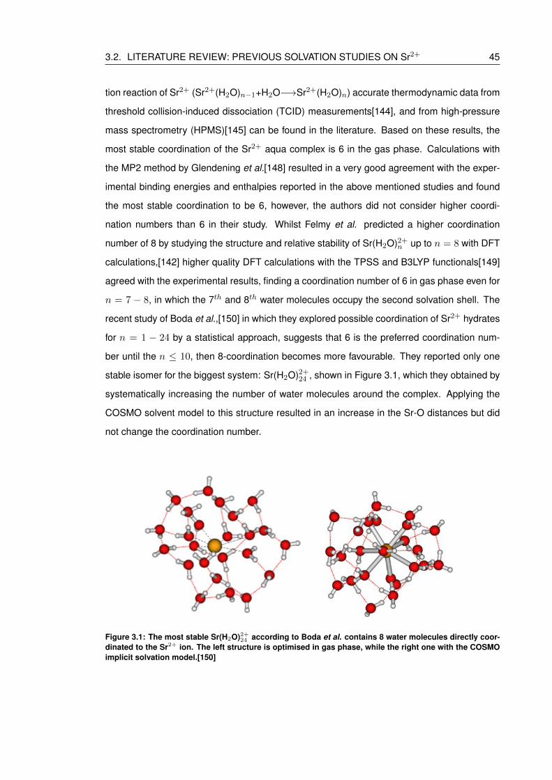
3.2. LITERATURE REVIEW: PREVIOUS SOLVATION STUDIES ON Sr2+ 45
tion reaction of Sr2+ (Sr2+(H2O)n−1+H2O−→Sr2+(H2O)n) accurate thermodynamic data from
threshold collision-induced dissociation (TCID) measurements[144], and from high-pressure
mass spectrometry (HPMS)[145] can be found in the literature. Based on these results, the
most stable coordination of the Sr2+ aqua complex is 6 in the gas phase. Calculations with
the MP2 method by Glendening et al.[148] resulted in a very good agreement with the exper-
imental binding energies and enthalpies reported in the above mentioned studies and found
the most stable coordination to be 6, however, the authors did not consider higher coordi-
nation numbers than 6 in their study. Whilst Felmy et al. predicted a higher coordination
number of 8 by studying the structure and relative stability of Sr(H2O)2+n up to n = 8 with DFT
calculations,[142] higher quality DFT calculations with the TPSS and B3LYP functionals[149]
agreed with the experimental results, finding a coordination number of 6 in gas phase even for
n = 7 − 8, in which the 7th and 8th water molecules occupy the second solvation shell. The
recent study of Boda et al.,[150] in which they explored possible coordination of Sr2+ hydrates
for n = 1 − 24 by a statistical approach, suggests that 6 is the preferred coordination num-
ber until the n ≤ 10, then 8-coordination becomes more favourable. They reported only one
stable isomer for the biggest system: Sr(H2O)2+24 , shown in Figure 3.1, which they obtained by
systematically increasing the number of water molecules around the complex. Applying the
COSMO solvent model to this structure resulted in an increase in the Sr-O distances but did
not change the coordination number.
Figure 3.1: The most stable Sr(H2O)2+24 according to Boda et al. contains 8 water molecules directly coor-dinated to the Sr2+ ion. The left structure is optimised in gas phase, while the right one with the COSMOimplicit solvation model.[150]
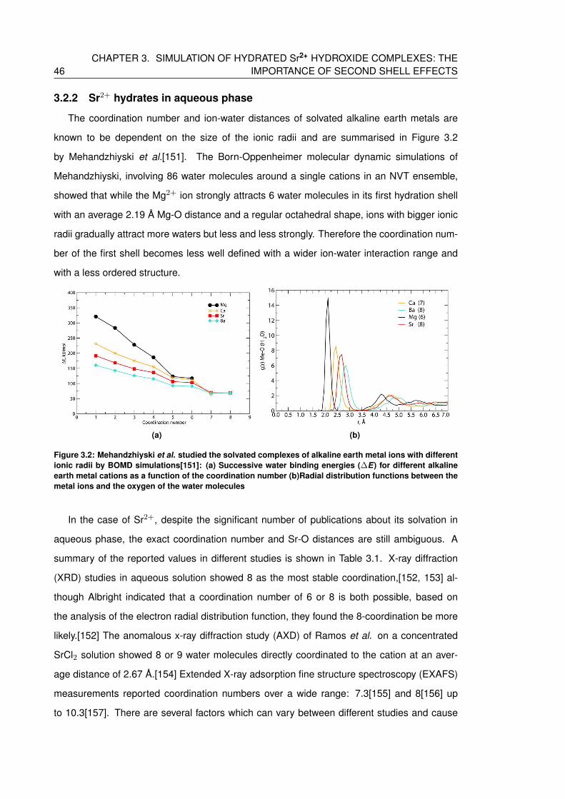
46CHAPTER 3. SIMULATION OF HYDRATED Sr2+ HYDROXIDE COMPLEXES: THE
IMPORTANCE OF SECOND SHELL EFFECTS
3.2.2 Sr2+ hydrates in aqueous phase
The coordination number and ion-water distances of solvated alkaline earth metals are
known to be dependent on the size of the ionic radii and are summarised in Figure 3.2
by Mehandzhiyski et al.[151]. The Born-Oppenheimer molecular dynamic simulations of
Mehandzhiyski, involving 86 water molecules around a single cations in an NVT ensemble,
showed that while the Mg2+ ion strongly attracts 6 water molecules in its first hydration shell
with an average 2.19 A Mg-O distance and a regular octahedral shape, ions with bigger ionic
radii gradually attract more waters but less and less strongly. Therefore the coordination num-
ber of the first shell becomes less well defined with a wider ion-water interaction range and
with a less ordered structure.
(a) (b)
Figure 3.2: Mehandzhiyski et al. studied the solvated complexes of alkaline earth metal ions with differentionic radii by BOMD simulations[151]: (a) Successive water binding energies (∆E) for different alkalineearth metal cations as a function of the coordination number (b)Radial distribution functions between themetal ions and the oxygen of the water molecules
In the case of Sr2+, despite the significant number of publications about its solvation in
aqueous phase, the exact coordination number and Sr-O distances are still ambiguous. A
summary of the reported values in different studies is shown in Table 3.1. X-ray diffraction
(XRD) studies in aqueous solution showed 8 as the most stable coordination,[152, 153] al-
though Albright indicated that a coordination number of 6 or 8 is both possible, based on
the analysis of the electron radial distribution function, they found the 8-coordination be more
likely.[152] The anomalous x-ray diffraction study (AXD) of Ramos et al. on a concentrated
SrCl2 solution showed 8 or 9 water molecules directly coordinated to the cation at an aver-
age distance of 2.67 A.[154] Extended X-ray adsorption fine structure spectroscopy (EXAFS)
measurements reported coordination numbers over a wide range: 7.3[155] and 8[156] up
to 10.3[157]. There are several factors which can vary between different studies and cause
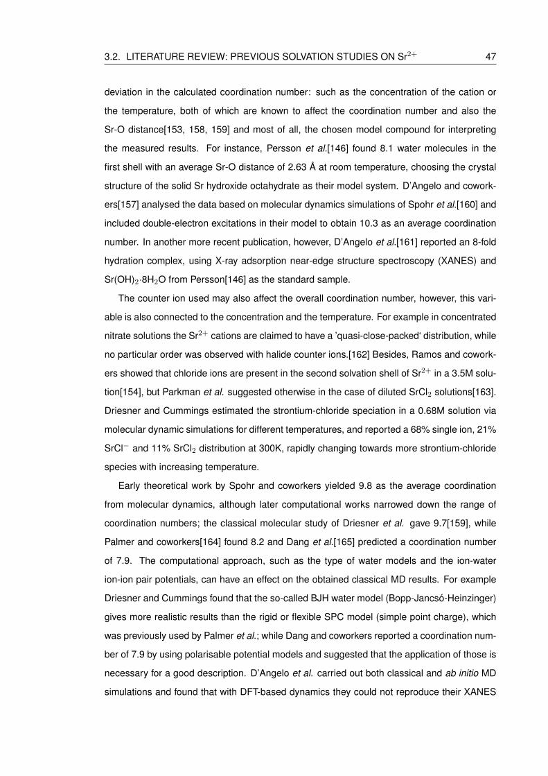
3.2. LITERATURE REVIEW: PREVIOUS SOLVATION STUDIES ON Sr2+ 47
deviation in the calculated coordination number: such as the concentration of the cation or
the temperature, both of which are known to affect the coordination number and also the
Sr-O distance[153, 158, 159] and most of all, the chosen model compound for interpreting
the measured results. For instance, Persson et al.[146] found 8.1 water molecules in the
first shell with an average Sr-O distance of 2.63 A at room temperature, choosing the crystal
structure of the solid Sr hydroxide octahydrate as their model system. D’Angelo and cowork-
ers[157] analysed the data based on molecular dynamics simulations of Spohr et al.[160] and
included double-electron excitations in their model to obtain 10.3 as an average coordination
number. In another more recent publication, however, D’Angelo et al.[161] reported an 8-fold
hydration complex, using X-ray adsorption near-edge structure spectroscopy (XANES) and
Sr(OH)2·8H2O from Persson[146] as the standard sample.
The counter ion used may also affect the overall coordination number, however, this vari-
able is also connected to the concentration and the temperature. For example in concentrated
nitrate solutions the Sr2+ cations are claimed to have a ’quasi-close-packed‘ distribution, while
no particular order was observed with halide counter ions.[162] Besides, Ramos and cowork-
ers showed that chloride ions are present in the second solvation shell of Sr2+ in a 3.5M solu-
tion[154], but Parkman et al. suggested otherwise in the case of diluted SrCl2 solutions[163].
Driesner and Cummings estimated the strontium-chloride speciation in a 0.68M solution via
molecular dynamic simulations for different temperatures, and reported a 68% single ion, 21%
SrCl− and 11% SrCl2 distribution at 300K, rapidly changing towards more strontium-chloride
species with increasing temperature.
Early theoretical work by Spohr and coworkers yielded 9.8 as the average coordination
from molecular dynamics, although later computational works narrowed down the range of
coordination numbers; the classical molecular study of Driesner et al. gave 9.7[159], while
Palmer and coworkers[164] found 8.2 and Dang et al.[165] predicted a coordination number
of 7.9. The computational approach, such as the type of water models and the ion-water
ion-ion pair potentials, can have an effect on the obtained classical MD results. For example
Driesner and Cummings found that the so-called BJH water model (Bopp-Jancso-Heinzinger)
gives more realistic results than the rigid or flexible SPC model (simple point charge), which
was previously used by Palmer et al.; while Dang and coworkers reported a coordination num-
ber of 7.9 by using polarisable potential models and suggested that the application of those is
necessary for a good description. D’Angelo et al. carried out both classical and ab initio MD
simulations and found that with DFT-based dynamics they could not reproduce their XANES

48CHAPTER 3. SIMULATION OF HYDRATED Sr2+ HYDROXIDE COMPLEXES: THE
IMPORTANCE OF SECOND SHELL EFFECTS
experimental data and obtained an outstandingly long Sr-O distance. However, other ab initio
MD simulations[24, 151, 166] predicted a coordination number from 6.7 to 7.5 with Sr-O dis-
tances well within the previously reported literature. Kerridge and Kaltsoyannis[149], similarly
to Boda et al., applied quantum chemical calculations with the COSMO solvent model on a
system containing 24 explicit water molecules and found a maximum coordination number of
7.
Table 3.1: Previously reported Sr2+ coordination numbers and Sr-O distances (A) in aqueous phase. Val-ues collected here are all measured or calculated at room temperature. XRD= X-ray diffraction, EXAFS=extended X-ray adsorption fine structure spectroscopy, LAXS= large angle X-ray scattering, XANES = x-ray adsorption near-edge structure spectroscopy, NRD= neutron diffraction and AXD = anomalous x-raydiffraction. (nw represents the number of water molecules in the reported simulations.)
Method Ref Solution CN d1(Sr-O) d2(Sr-O) Used standard / Computational details
XRD Albright[152] concentrated SrCl2 8 2.6XRD Caminiti[153] 2M SrCl2 8 2.64 4.94
XRD/Raman Cabaco[162] 2.7M Sr(NO3)2 8 2.64
EXAFS Pfund[155] 0.2M Sr(NO3)2 7.3 2.62 SrO powderEXAFS Palmer[164] SrCl2 7.7 2.63 SrO powder/MDEXAFS Seward[158] 0.1M SrCl2 7.8 2.57 classical MDEXAFS Moreau[156] 0.14M Sr(O3SCF3)2 8 2.600 Sr(H2O)8(OH)2[146]
LAXS/EXAFS Persson[146] 0.1M Sr(CF3SO3)2 8 2.63 4.780 Sr(H2O)8(OH)2EXAFS Parkman[163] 0.1M SrCl2 8.3 2.62 -EXAFS Axe[167] 0.05M Sr(NO3)2 8.93 2.62 SrO powderEXAFS D’Angelo[157] 3.0M SrCl2 10.3 2.643 classical MD[160]XANES D’Angelo[161] 0.2M Sr(H2O)8(OH)2 8 2.6 Sr(H2O)8(OH)2
NRD Neilson[168] 3M Sr(ClO4)2xD2O - 2.3-2.65
AXD Ramos[154] 3.5M SrCl2 8-9 2.67 4.97
classical MD Spohr[160] 1.1M SrCl2 nw=200 9.8 2.63H2O: Central Force model,
Sr2+, Cl− parametrisedbased on HF calculations
classical MD Driesner[159] 0.5M SrCl2 nw=250 (NVT) 9.7 2.64 4.92H2O: BJH model,
Sr2+, Cl− from Spohr[160]
classical MD Boda[150] 0.1M SrCl2 nw=511 (NPT) 8.24 2.58 4.82H2O: TIP4P model,
PPPM method
classical MD Palmer[164] ∼0.2M SrCl2 nw=253 8.2 2.57H2O: SPC/E model,
Sr2+: parameters by Dang[164]
classical MD D’Angelo[161] 0.05 Sr2+(aq) nw=819 (NVT) 8 2.60 4.78H2O: SPC/E model,
Sr2+: parameters by Aqvist[169]
classical MD Dang[165] nw=600 (NPT) 7.9 2.60H2O: SPC/E model,
Sr2+: parameters by Dang
QM/MM Hofer[170] 0.11M SrCl2 nw=499 (NVT) 9 2.69 4.97QM: HF-SCF/DZP rQM=3.9 A
MM: potentials constructedbased on HF calculations
BOMD Harris[166] Sr(H2O)2+n nw=30 (NVT) 7.5 2.6 PBE/USPP-PW
BOMD Mehandzhiyski[151] Sr(H2O)2+n nw=86 (NVT) 7-8 2.67 4.6 BLYP-D/GWP-DZVP-GTH
CPMD D’Angelo[161] Sr(H2O)2+n nw=90 (NVT) 7.5 2.72 4.92 revPBE/DCACPs
CPMD Di Tommaso[24] Sr(H2O)2+n nw=53 (NVT) 6.7 2.60 4.70 PBE/USPP-PW
DFT/MP2(COSMO) Boda[150] Sr(H2O)2+n nw=24 8 2.64 B3LYP/TZVP and MP2/TZVP
DFT(COSMO) Kerridge[149] Sr(H2O)2+n nw=24 7 2.614 TPSS/def2-TZVP
3.2.3 The order and dynamics of hydration shells
Neilson and Broadbent[168] used neutron diffraction to study the structure of Sr2+ in a
highly concentrated Sr(ClO4)2 solution in heavy water, but they were not able to resolve the
water structure around the ion into Sr-O and Sr-H correlations, due to the disordered structure
of the first solvation shell. Moreau,[156] Axe[167] and Persson[146] also concluded that the
inner solvation shell of the Sr2+ is highly disordered and the outer shell is diffuse, which could
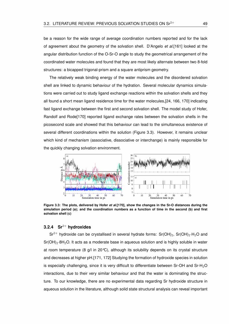
3.2. LITERATURE REVIEW: PREVIOUS SOLVATION STUDIES ON Sr2+ 49
be a reason for the wide range of average coordination numbers reported and for the lack
of agreement about the geometry of the solvation shell. D’Angelo et al.[161] looked at the
angular distribution function of the O-Sr-O angle to study the geometrical arrangement of the
coordinated water molecules and found that they are most likely alternate between two 8-fold
structures: a bicapped trigonal-prism and a square antiprism geometry.
The relatively weak binding energy of the water molecules and the disordered solvation
shell are linked to dynamic behaviour of the hydration. Several molecular dynamics simula-
tions were carried out to study ligand exchange reactions within the solvation shells and they
all found a short mean ligand residence time for the water molecules,[24, 166, 170] indicating
fast ligand exchange between the first and second solvation shell. The model study of Hofer,
Randolf and Rode[170] reported ligand exchange rates between the solvation shells in the
picosecond scale and showed that this behaviour can lead to the simultaneous existence of
several different coordinations within the solution (Figure 3.3). However, it remains unclear
which kind of mechanism (associative, dissociative or interchange) is mainly responsible for
the quickly changing solvation environment.
Figure 3.3: The plots, delivered by Hofer et al.[170], show the changes in the Sr-O distances during thesimulation period (a); and the coordination numbers as a function of time in the second (b) and firstsolvation shell (c)
3.2.4 Sr2+ hydroxides
Sr2+ hydroxide can be crystallised in several hydrate forms: Sr(OH)2, Sr(OH)2·H2O and
Sr(OH)2·8H2O. It acts as a moderate base in aqueous solution and is highly soluble in water
at room temperature (8 g/l in 20°C), although its solubility depends on its crystal structure
and decreases at higher pH.[171, 172] Studying the formation of hydroxide species in solution
is especially challenging, since it is very difficult to differentiate between Sr-OH and Sr-H2O
interactions, due to their very similar behaviour and that the water is dominating the struc-
ture. To our knowledge, there are no experimental data regarding Sr hydroxide structure in
aqueous solution in the literature, although solid state structural analysis can reveal important
50CHAPTER 3. SIMULATION OF HYDRATED Sr2+ HYDROXIDE COMPLEXES: THE
IMPORTANCE OF SECOND SHELL EFFECTS
information to aid understanding of solvation. XRD data of Grueninger and Barnighausen
have shown that anhydrous Sr(OH)2 has a polyhedral coordination in which the Sr2+ ion is
surrounded by seven OH− ions with Sr-O distances between 2.496-2.767 A (average of 2.60
A).[147] Strontium hydroxide monohydrate is reported to be relatively unstable, partially de-
composing to the anhydrous hydroxide by prolonged exposition at room temperature.[173] Its
structure was intensively studied with IR and Raman single crystal measurements by Lutz et
al.[174, 175] and reported to have a hydroxide coordination in a trigonal prismatic structure
around the Sr2+ ion, bicapped by the oxygen atoms of the water molecules. IR and Raman
spectra reveal that in such formations, coordinating waters are strongly hydrogen bonded
but, by contrast, the hydroxide ions do not act as hydrogen-bond donors at all, presumably
because water molecules are much stronger hydrogen bond donors than hydroxide ions in
general.[175] Sr(OH)2·8H2O has an entirely different structure; it contains hydrogen donating
OH− ions. Based on XRD,[146, 176] and neutron diffraction studies[177] oxygen atoms from
eight water molecules coordinate the Sr2+ ion in a tetragonal antiprismatic conformation, with
each water engaged at least in three hydrogen bonds. According to Ricci et al.[177] a signif-
icant difference can be detected in the length of the O-H bonds within the water molecules,
which makes their structure asymmetric in the crystal: the longer bonds are H-bond donors to
OH− ions (∼ 1.005 A), while the shorter ones are donors to another water molecule (∼ 0.975
A). The hydroxide ions in solid Sr(OH)2·8H2O are not coordinated directly to the Sr2+ centre,
but instead form chains of acceptor and donor bonds, with each hydroxide oxygen involved in
four hydrogen bonds with neighbouring waters.[146]
Only gas phase theoretical studies exist concerning the hydrolysis of Sr2+. Felmy et
al.[142] introduced a hydroxide ion into hydrate complexes by removal of a proton from Sr(H2O)2+6
and Sr(H2O)2+8 . The obtained monohydroxide structures are shown in Figure 3.4. Interest-
ingly, they found that the addition of water molecules to the system dissociates the hydroxide
ion from the central ion, i.e. in Sr(H2O)7(OH)+ the OH− ion is not directly connected to the
Sr2+; instead, it has three hydrogen bonds to water molecules in the primary solvation shell.
This result suggests only weak hydrolysis of aqueous Sr2+, although the authors note that
the delocalization of the hydroxide ion may be overestimated in the gas phase compared
with aqueous phase calculations due to the lack of a background potential and/or competitive
explicit second shell water molecules.
Kerridge et al.[122] published a more detailed investigation of the hydroxide complexes
of Sr2+ in 2011, in which they studied a series of Sr(H2O)(8−n)(OH)(2−n)+n complexes up to
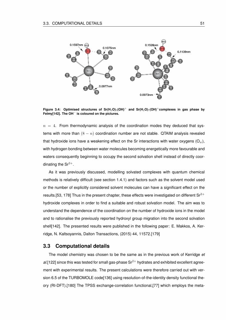
3.3. COMPUTATIONAL DETAILS 51
Figure 3.4: Optimised structures of Sr(H2O)5(OH)+ and Sr(H2O)7(OH)+complexes in gas phase byFelmy[142]. The OH− is coloured on the pictures.
n = 4. From thermodynamic analysis of the coordination modes they deduced that sys-
tems with more than (8 − n) coordination number are not stable. QTAIM analysis revealed
that hydroxide ions have a weakening effect on the Sr interactions with water oxygens (Ow),
with hydrogen bonding between water molecules becoming energetically more favourable and
waters consequently beginning to occupy the second solvation shell instead of directly coor-
dinating the Sr2+.
As it was previously discussed, modelling solvated complexes with quantum chemical
methods is relatively difficult (see section 1.4.1) and factors such as the solvent model used
or the number of explicitly considered solvent molecules can have a significant effect on the
results.[53, 178] Thus in the present chapter, these effects were investigated on different Sr2+
hydroxide complexes in order to find a suitable and robust solvation model. The aim was to
understand the dependence of the coordination on the number of hydroxide ions in the model
and to rationalise the previously reported hydroxyl group migration into the second solvation
shell[142]. The presented results were published in the following paper: E. Makkos, A. Ker-
ridge, N. Kaltsoyannis, Dalton Transactions, (2015) 44, 11572.[179]
3.3 Computational detailsThe model chemistry was chosen to be the same as in the previous work of Kerridge et
al.[122] since this was tested for small gas-phase Sr2+ hydrates and exhibited excellent agree-
ment with experimental results. The present calculations were therefore carried out with ver-
sion 6.5 of the TURBOMOLE code[136] using resolution-of-the-identity density functional the-
ory (RI-DFT).[180] The TPSS exchange-correlation functional,[77] which employs the meta-
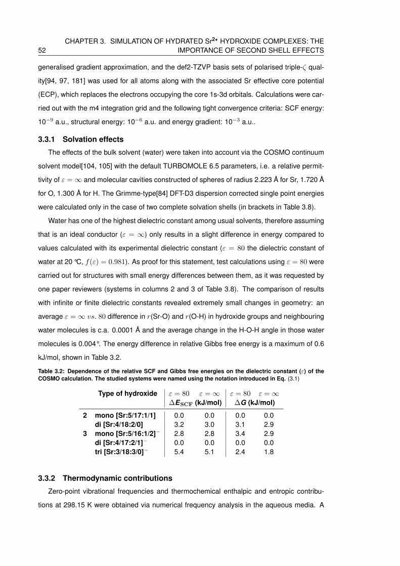
52CHAPTER 3. SIMULATION OF HYDRATED Sr2+ HYDROXIDE COMPLEXES: THE
IMPORTANCE OF SECOND SHELL EFFECTS
generalised gradient approximation, and the def2-TZVP basis sets of polarised triple-ζ qual-
ity[94, 97, 181] was used for all atoms along with the associated Sr effective core potential
(ECP), which replaces the electrons occupying the core 1s-3d orbitals. Calculations were car-
ried out with the m4 integration grid and the following tight convergence criteria: SCF energy:
10−9 a.u., structural energy: 10−6 a.u. and energy gradient: 10−3 a.u..
3.3.1 Solvation effects
The effects of the bulk solvent (water) were taken into account via the COSMO continuum
solvent model[104, 105] with the default TURBOMOLE 6.5 parameters, i.e. a relative permit-
tivity of ε =∞ and molecular cavities constructed of spheres of radius 2.223 A for Sr, 1.720 A
for O, 1.300 A for H. The Grimme-type[84] DFT-D3 dispersion corrected single point energies
were calculated only in the case of two complete solvation shells (in brackets in Table 3.8).
Water has one of the highest dielectric constant among usual solvents, therefore assuming
that is an ideal conductor (ε = ∞) only results in a slight difference in energy compared to
values calculated with its experimental dielectric constant (ε = 80 the dielectric constant of
water at 20 °C, f(ε) = 0.981). As proof for this statement, test calculations using ε = 80 were
carried out for structures with small energy differences between them, as it was requested by
one paper reviewers (systems in columns 2 and 3 of Table 3.8). The comparison of results
with infinite or finite dielectric constants revealed extremely small changes in geometry: an
average ε =∞ vs. 80 difference in r(Sr-O) and r(O-H) in hydroxide groups and neighbouring
water molecules is c.a. 0.0001 A and the average change in the H-O-H angle in those water
molecules is 0.004°. The energy difference in relative Gibbs free energy is a maximum of 0.6
kJ/mol, shown in Table 3.2.
Table 3.2: Dependence of the relative SCF and Gibbs free energies on the dielectric constant (ε) of theCOSMO calculation. The studied systems were named using the notation introduced in Eq. (3.1)
Type of hydroxide ε = 80 ε =∞ ε = 80 ε =∞∆ESCF (kJ/mol) ∆G (kJ/mol)
2 mono [Sr:5/17:1/1] 0.0 0.0 0.0 0.0di [Sr:4/18:2/0] 3.2 3.0 3.1 2.9
3 mono [Sr:5/16:1/2]− 2.8 2.8 3.4 2.9di [Sr:4/17:2/1]− 0.0 0.0 0.0 0.0tri [Sr:3/18:3/0]− 5.4 5.1 2.4 1.8
3.3.2 Thermodynamic contributions
Zero-point vibrational frequencies and thermochemical enthalpic and entropic contribu-
tions at 298.15 K were obtained via numerical frequency analysis in the aqueous media. A
3.4. RESULTS 53
frequency scaling factor of 1 was used throughout, since according to test calculations with
the TPSS functional and a basis set of similar quality to that employed here (6-311G(d,p))
a scaling factor of 0.9999 was found to be appropriate in order to minimise the RMS error of
the zero-point vibrational energies (ZPVEs).[182] Results were visualised with the MOLDRAW
chemical graphical software[183–185].
3.4 Results
In this section we present the results of quantum chemical calculations in which a combi-
nation of the COSMO implicit solvent model and explicit solvent molecules was used to study
the aqueous solvation of strontium mono-, di-, tri-, and tetrahydroxides. The following labelling
scheme is employed to classify the studied systems:
[Sr : a/b : α/β](2−n)+ (3.1)
a and b are the numbers of explicit waters in the first and second shell, respectively, α and
β are the corresponding number of hydroxyl groups, and n is the total number of OH− ions in
the system. For instance, the structure labelled [Sr:5/17:1/1] is a neutral, 6 coordinated Sr2+
monohydroxide with five water molecules and one OH− ion in the first shell, and 17 waters
and one OH− ion in the second.
3.4.1 Sr2+ hydroxide complexes with a first solvation shell
Previous gas phase studies have identified the maximum coordination number of Sr2+
hydroxide complexes to be seven, with a tendency to decrease with increasing number of
OH− ions in the system.[122] Therefore, we kept the total number of molecules in the system
at seven and studied structures with one to four hydroxyl groups while the number of explicit
waters was reduced concurrently from six to three. A continuum solvent model was employed
in all cases.
We attempted to map all possible coordinations while keeping the number of waters and
OH− ions constant in the system. However, despite repeated efforts, we were unable to sta-
bilise complexes with certain coordination numbers. Hence the following complexes are ab-
sent from our study: [Sr:4/2:1/0]+, [Sr:5/1:1/0]+, [Sr:6/0:1/0]+, [Sr:5/0:2/0] and [Sr:3/0:4/0]2−.
Attempts to optimise these structures resulted in imaginary frequencies which proved impossi-
ble to eliminate. For all other complexes, optimised structures together with their relative SCF
and Gibbs energies (∆ESCF/∆G) are summarised in Table 3.3. Relative energies were calcu-
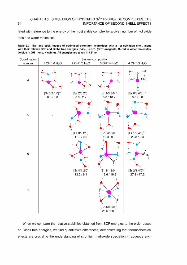
54CHAPTER 3. SIMULATION OF HYDRATED Sr2+ HYDROXIDE COMPLEXES: THE
IMPORTANCE OF SECOND SHELL EFFECTS
lated with reference to the energy of the most stable complex for a given number of hydroxide
ions and water molecules.
Table 3.3: Ball and stick images of optimised strontium hydroxides with a 1st solvation shell, alongwith their relative SCF and Gibbs free energies (∆ESCF/∆G). (Sr2+=magenta, O=red in water molecules,O=blue in OH− ions, H=white). All energies are given in kJ/mol
Coordinationnumber
System composition1 OH−/6 H2O 2 OH−/5 H2O 3 OH−/4 H2O 4 OH−/3 H2O
4
[Sr:3/3:1/0]+ [Sr:2/3:2/0] [Sr:1/3:3/0]− [Sr:0/3:4/0]2−
0.0 / 0.0 0.0 / 2.7 0.0 / 10.2 0.0 / 0.0
5 -
[Sr:3/2:2/0] [Sr:2/2:3/0]− [Sr:1/2:4/0]2−
11.3 / 0.0 10.3 / 0.0 28.3 / 8.3
6 -
[Sr:4/1:2/0] [Sr:3/1:3/0]− [Sr:2/1:4/0]2−
13.5 / 9.1 16.6 / 19.9 27.8 / 17.2
7 - - -
[Sr:4/0:3/0]−
26.5 / 28.9
When we compare the relative stabilities obtained from SCF energies to the order based
on Gibbs free energies, we find quantitative differences, demonstrating that thermochemical
effects are crucial to the understanding of strontium hydroxide speciation in aqueous envi-
3.4. RESULTS 55
ronments. Considering the ∆G results, the most stable coordination number is five for the
di- and trihydroxide complexes ([Sr:3/2:2/0] and [Sr:2/2:3/0]−), while it is four for the tetrahy-
droxides ([Sr:0/3:4/0]2−). These results are in partial agreement with the previous gas phase
study[122] in which the maximum coordination number of seven decreases to four with an
increasing number of hydroxide ions. Furthermore, the reduction in total coordination number
from five to four found here is consistent with the previous observation from QTAIM analysis
that increasing the number of hydroxide ions destabilises higher coordinations.
Inspection of Table 3.3 reveals that for most species, large parts of the first coordination
sphere are open, an unphysical situation which would not be possible in real solvated systems.
This, and the problems we encountered with energetic instability in several structures, led
us to conclude that the combination of an implicit bulk solvent and explicit first coordination
shell does not contain enough explicit coordination to accurately model the solvation of Sr2+
hydroxides. To overcome this problem, we moved on to study the effect of using additional
explicit waters in our solvation model.
3.4.2 Sr2+ hydroxide complexes with a first and second solvation shells
When deciding on the total number of water molecules required to complete two solvation
shells, we took into account the possibility that the hydroxide ions can in principle migrate to
the second shell, in which case it would be possible to form an eight coordinated hydrate com-
plex.[146] Therefore we chose the maximum number of water molecules to be 24-n, (where n
is the number of hydroxide ions in the system) considering that only two second shell waters
are able to coordinate each first shell water.
We attempted to create complexes with a second solvation shell by two different approach:
by systematically increasing the number of water molecules around the previously optimised
‘single shell’ complexes and by using a pre-optimised water cluster as solvation shell. While
the first approach is more common and was used by Boda et al.[150], the latter one was also
successfully used before to model the effect of first solvation shell for organic reactions.[186,
187] We applied a 24 water molecule cluster (W24) previously optimised by Ludwig and Wein-
hold, as a starting point.[188] These authors found that a tetrakaidecahedral cluster composed
of two hexagons and twelve pentagons was energetically most stable (see Figure 3.5) and it
was confirmed by later conformation studies too.[189] For modelling the solvation of Sr2+ hy-
droxides, we modified this cluster by placing a Sr2+ ion at its centre and replacing between
one and four waters with hydroxide ions.

56CHAPTER 3. SIMULATION OF HYDRATED Sr2+ HYDROXIDE COMPLEXES: THE
IMPORTANCE OF SECOND SHELL EFFECTS
(a) side view (b) top view
Figure 3.5: Optimised structure of the W24 water cluster reported by Ludwig and Weinhold[190]
To verify the suitability of the chosen water cluster for this particular problem, we first stud-
ied simple Sr2+ hydrates. We found 6 and 7 coordinated aqua complexes to be energetically
very similar; the 6 coordinated structure is 6.0 kJ/mol more favoured based on the SCF en-
ergies,and Gibbs free energies show that both coordination is equally likely (see Figure 3.6).
These results are at the lower end of the previously published coordination range (shown in
Table 3.1)[155, 158, 164] and in a relatively good agreement with the existing quantum chem-
ical results in which the preferred coordination was seven.[24, 149, 151, 161, 166]
(a) [Sr:6/18:0/0]2+
0.0 / 0.0(b) [Sr:7/17:0/0]2+
6.0 / 0.0
Figure 3.6: Optimised structures of two Sr2+ hydrates with a first solvation shell (ball and stick) sur-rounded by an explicit second solvation shell (represented as tubes), along with their relative SCF andfree energies (∆ESCF /∆G). (Sr2+=magenta, O=red in water molecules, H=white). Energies are given inkJ/mol.
Table 3.4, 3.5, 3.6 and 3.7 compare all obtained structures by both methods containing
1,2,3 or 4 OH− ions in the system respectively. Complexes which were optimised based on
the W24 water cluster, all have names starting with W24 OH x, while structures obtained by
introducing water molecules one-by-one around the 1st shell complexes are called such as
C1m x, C1g x etc. We found, that the ”built-up” structures, with the exception of systems
containing single OH− ion (W24 OH1 and C1c 23b in Table 3.4), were always energetically
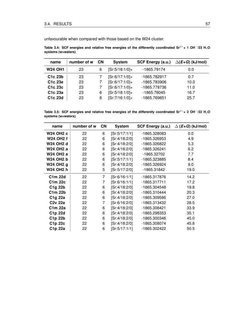
3.4. RESULTS 57
unfavourable when compared with those based on the W24 cluster.
Table 3.4: SCF energies and relative free energies of the differently coordinated Sr2++ 1 OH−/23 H2Osystems (w=waters)
name number of w CN System SCF Energy (a.u.) ∆(E+G) (kJ/mol)
W24 OH1 23 6 [Sr:5/18:1/0]+ -1865.79174 0.0
C1c 23b 23 7 [Sr:6/17:1/0]+ -1865.782917 0.7C1c 23e 23 7 [Sr:6/17:1/0]+ -1865.783906 10.0C1c 23c 23 7 [Sr:6/17:1/0]+ -1865.778736 11.0C1c 23a 23 6 [Sr:5/18:1/0]+ -1865.78045 16.7C1c 23d 23 8 [Sr:7/16:1/0]+ -1865.769851 25.7
Table 3.5: SCF energies and relative free energies of the differently coordinated Sr2++ 2 OH−/22 H2Osystems (w=waters)
name number of w CN System SCF Energy (a.u.) ∆ (E+G) (kJ/mol)
W24 OH2 c 22 6 [Sr:5/17:1/1] -1865.328083 0.0W24 OH2 f 22 6 [Sr:4/18:2/0] -1865.326953 4.9W24 OH2 d 22 6 [Sr:4/18:2/0] -1865.326822 5.3W24 OH2 a 22 6 [Sr:4/18:2/0] -1865.326241 6.2W24 OH2 e 22 6 [Sr:4/18:2/0] -1865.32702 7.7W24 OH2 b 22 6 [Sr:5/17:1/1] -1865.323885 8.4W24 OH2 g 22 6 [Sr:4/18:2/0] -1865.326924 9.0W24 OH2 h 22 5 [Sr:5/17:2/0] -1865.31842 19.0
C1m 22d 22 7 [Sr:6/16:1/1] -1865.317876 14.2C1m 22c 22 7 [Sr:6/16:1/1] -1865.317711 17.2C1g 22b 22 6 [Sr:4/18:2/0] -1865.304548 19.8C1m 22b 22 6 [Sr:4/18:2/0] -1865.310444 20.3C1g 22a 22 6 [Sr:4/18:2/0] -1865.309586 27.0C2v 22a 22 7 [Sr:6/16:2/0] -1865.313432 28.5C1m 22a 22 6 [Sr:4/18:2/0] -1865.308421 33.9C1p 22d 22 6 [Sr:4/18:2/0] -1865.298353 35.1C1p 22b 22 6 [Sr:4/18:2/0] -1865.300346 45.0C1p 22c 22 6 [Sr:4/18:2/0] -1865.308074 45.8C1p 22a 22 6 [Sr:5/17:1/1] -1865.302422 50.5
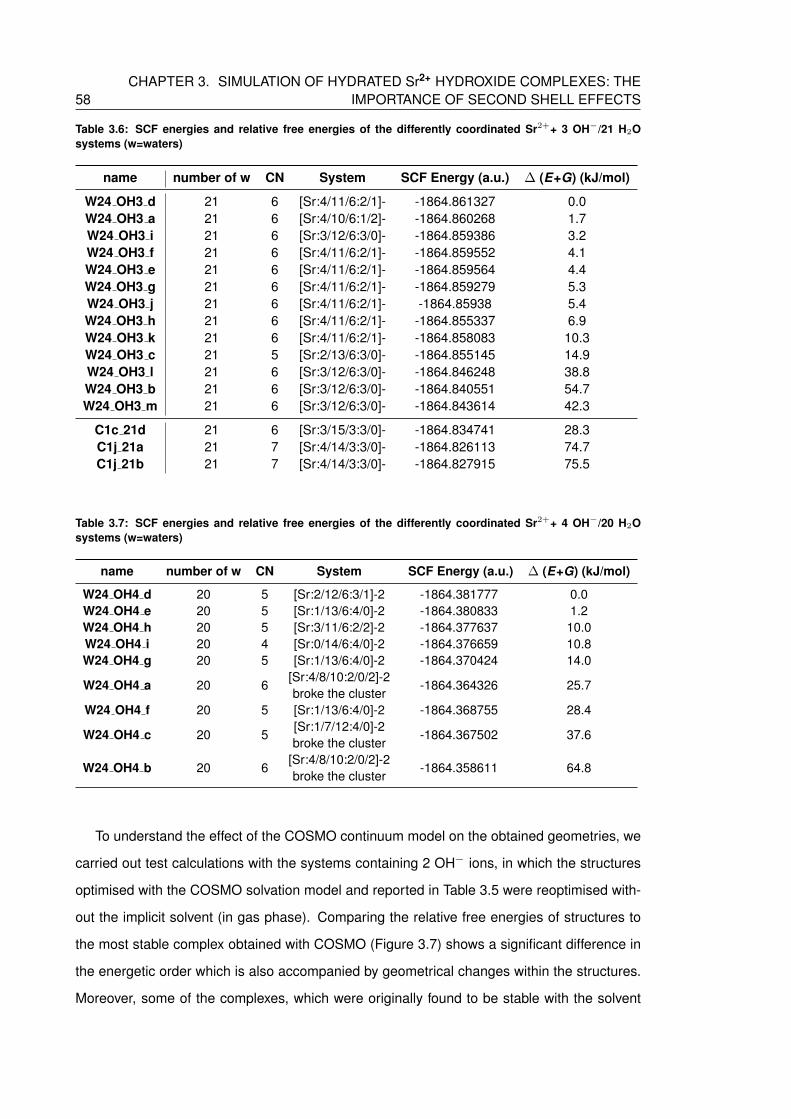
58CHAPTER 3. SIMULATION OF HYDRATED Sr2+ HYDROXIDE COMPLEXES: THE
IMPORTANCE OF SECOND SHELL EFFECTS
Table 3.6: SCF energies and relative free energies of the differently coordinated Sr2++ 3 OH−/21 H2Osystems (w=waters)
name number of w CN System SCF Energy (a.u.) ∆ (E+G) (kJ/mol)
W24 OH3 d 21 6 [Sr:4/11/6:2/1]- -1864.861327 0.0W24 OH3 a 21 6 [Sr:4/10/6:1/2]- -1864.860268 1.7W24 OH3 i 21 6 [Sr:3/12/6:3/0]- -1864.859386 3.2W24 OH3 f 21 6 [Sr:4/11/6:2/1]- -1864.859552 4.1W24 OH3 e 21 6 [Sr:4/11/6:2/1]- -1864.859564 4.4W24 OH3 g 21 6 [Sr:4/11/6:2/1]- -1864.859279 5.3W24 OH3 j 21 6 [Sr:4/11/6:2/1]- -1864.85938 5.4W24 OH3 h 21 6 [Sr:4/11/6:2/1]- -1864.855337 6.9W24 OH3 k 21 6 [Sr:4/11/6:2/1]- -1864.858083 10.3W24 OH3 c 21 5 [Sr:2/13/6:3/0]- -1864.855145 14.9W24 OH3 l 21 6 [Sr:3/12/6:3/0]- -1864.846248 38.8W24 OH3 b 21 6 [Sr:3/12/6:3/0]- -1864.840551 54.7W24 OH3 m 21 6 [Sr:3/12/6:3/0]- -1864.843614 42.3
C1c 21d 21 6 [Sr:3/15/3:3/0]- -1864.834741 28.3C1j 21a 21 7 [Sr:4/14/3:3/0]- -1864.826113 74.7C1j 21b 21 7 [Sr:4/14/3:3/0]- -1864.827915 75.5
Table 3.7: SCF energies and relative free energies of the differently coordinated Sr2++ 4 OH−/20 H2Osystems (w=waters)
name number of w CN System SCF Energy (a.u.) ∆ (E+G) (kJ/mol)
W24 OH4 d 20 5 [Sr:2/12/6:3/1]-2 -1864.381777 0.0W24 OH4 e 20 5 [Sr:1/13/6:4/0]-2 -1864.380833 1.2W24 OH4 h 20 5 [Sr:3/11/6:2/2]-2 -1864.377637 10.0W24 OH4 i 20 4 [Sr:0/14/6:4/0]-2 -1864.376659 10.8W24 OH4 g 20 5 [Sr:1/13/6:4/0]-2 -1864.370424 14.0
W24 OH4 a 20 6[Sr:4/8/10:2/0/2]-2broke the cluster
-1864.364326 25.7
W24 OH4 f 20 5 [Sr:1/13/6:4/0]-2 -1864.368755 28.4
W24 OH4 c 20 5[Sr:1/7/12:4/0]-2broke the cluster
-1864.367502 37.6
W24 OH4 b 20 6[Sr:4/8/10:2/0/2]-2broke the cluster
-1864.358611 64.8
To understand the effect of the COSMO continuum model on the obtained geometries, we
carried out test calculations with the systems containing 2 OH− ions, in which the structures
optimised with the COSMO solvation model and reported in Table 3.5 were reoptimised with-
out the implicit solvent (in gas phase). Comparing the relative free energies of structures to
the most stable complex obtained with COSMO (Figure 3.7) shows a significant difference in
the energetic order which is also accompanied by geometrical changes within the structures.
Moreover, some of the complexes, which were originally found to be stable with the solvent
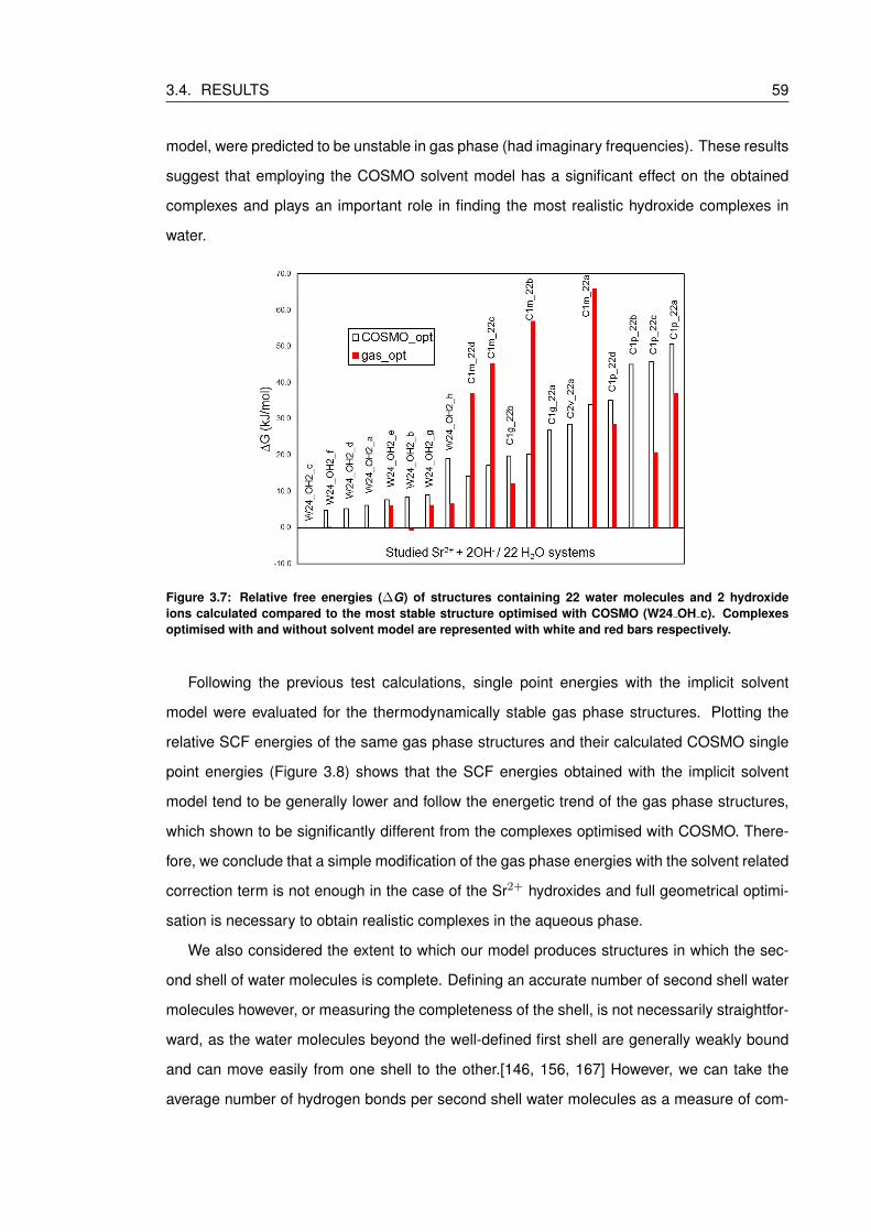
3.4. RESULTS 59
model, were predicted to be unstable in gas phase (had imaginary frequencies). These results
suggest that employing the COSMO solvent model has a significant effect on the obtained
complexes and plays an important role in finding the most realistic hydroxide complexes in
water.
Figure 3.7: Relative free energies (∆G) of structures containing 22 water molecules and 2 hydroxideions calculated compared to the most stable structure optimised with COSMO (W24 OH c). Complexesoptimised with and without solvent model are represented with white and red bars respectively.
Following the previous test calculations, single point energies with the implicit solvent
model were evaluated for the thermodynamically stable gas phase structures. Plotting the
relative SCF energies of the same gas phase structures and their calculated COSMO single
point energies (Figure 3.8) shows that the SCF energies obtained with the implicit solvent
model tend to be generally lower and follow the energetic trend of the gas phase structures,
which shown to be significantly different from the complexes optimised with COSMO. There-
fore, we conclude that a simple modification of the gas phase energies with the solvent related
correction term is not enough in the case of the Sr2+ hydroxides and full geometrical optimi-
sation is necessary to obtain realistic complexes in the aqueous phase.
We also considered the extent to which our model produces structures in which the sec-
ond shell of water molecules is complete. Defining an accurate number of second shell water
molecules however, or measuring the completeness of the shell, is not necessarily straightfor-
ward, as the water molecules beyond the well-defined first shell are generally weakly bound
and can move easily from one shell to the other.[146, 156, 167] However, we can take the
average number of hydrogen bonds per second shell water molecules as a measure of com-
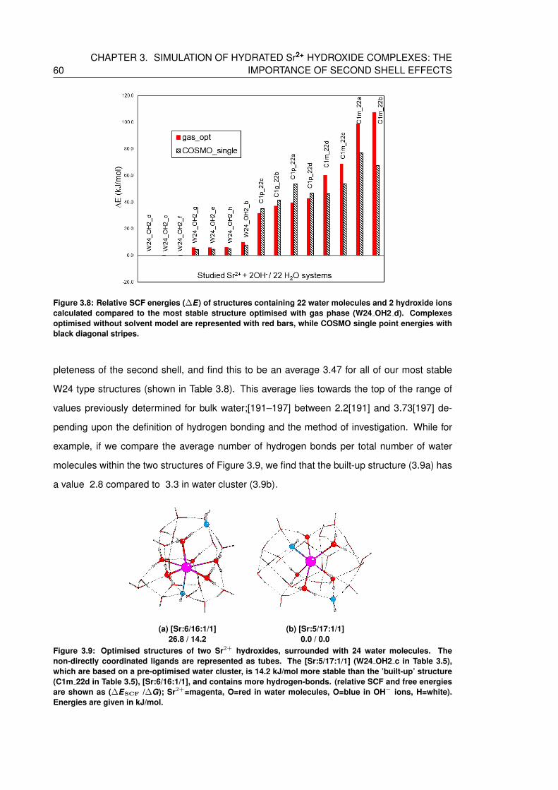
60CHAPTER 3. SIMULATION OF HYDRATED Sr2+ HYDROXIDE COMPLEXES: THE
IMPORTANCE OF SECOND SHELL EFFECTS
Figure 3.8: Relative SCF energies (∆E) of structures containing 22 water molecules and 2 hydroxide ionscalculated compared to the most stable structure optimised with gas phase (W24 OH2 d). Complexesoptimised without solvent model are represented with red bars, while COSMO single point energies withblack diagonal stripes.
pleteness of the second shell, and find this to be an average 3.47 for all of our most stable
W24 type structures (shown in Table 3.8). This average lies towards the top of the range of
values previously determined for bulk water;[191–197] between 2.2[191] and 3.73[197] de-
pending upon the definition of hydrogen bonding and the method of investigation. While for
example, if we compare the average number of hydrogen bonds per total number of water
molecules within the two structures of Figure 3.9, we find that the built-up structure (3.9a) has
a value 2.8 compared to 3.3 in water cluster (3.9b).
(a) [Sr:6/16:1/1]26.8 / 14.2
(b) [Sr:5/17:1/1]0.0 / 0.0
Figure 3.9: Optimised structures of two Sr2+ hydroxides, surrounded with 24 water molecules. Thenon-directly coordinated ligands are represented as tubes. The [Sr:5/17:1/1] (W24 OH2 c in Table 3.5),which are based on a pre-optimised water cluster, is 14.2 kJ/mol more stable than the ’built-up’ structure(C1m 22d in Table 3.5), [Sr:6/16:1/1], and contains more hydrogen-bonds. (relative SCF and free energiesare shown as (∆ESCF /∆G); Sr2+=magenta, O=red in water molecules, O=blue in OH− ions, H=white).Energies are given in kJ/mol.

3.4. RESULTS 61
Presumably the high symmetry of the W24 cluster and the closed hydrogen bond network
stabilises the systems obtained from this approach. Since the W24 cluster based complexes
are generally more stable and have more complete second shell than the ’built-up’ structures,
we concluded that the use of the pre-optimised cluster approach provides an appropriate
starting point from which to model two complete solvation shells and after this point only the
W24 cluster based results are presented in this chapter and summarised in Table 3.8. Relative
energies are calculated compared to the most stable structures for a given number of OH−
ions and waters in the system.
Table 3.8: Optimised structures with a first solvation shell (ball and stick) surrounded by an explicit secondsolvation shell (represented as tubes), along with their relative SCF, dispersion corrected and free energies(∆ESCF (∆ED3) /∆G). (Sr2+=magenta, O=red in water molecules, O=blue in OH− ions, H=white). Allenergies are given in kJ/mol.
Hydroxidecoordination
System composition1 OH−/23 H2O 2 OH−/22 H2O 3 OH−/21 H2O 4 OH−/20 H2O
mono -
[Sr:5/18:1/0]+ [Sr:5/17:1/1] [Sr:5/16:1/2]−
0.0 (0.0) / 0.0 0.0 (0.0) / 0.0 2.8 (1.8)/ 2.9
di -
[Sr:4/18:2/0] [Sr:4/17:2/1]− [Sr:4/16:2/2]2−
3.0 (4.4) / 2.9 0.0 (0.0) / 0.0 10.9 (9.0) / 10.1
tri - -
[Sr:3/18:3/0]− [Sr:2/18:3/1]2−
5.1 (6.9) / 1.8 0.0 (0.0) / 0.0
tetra - - -
[Sr:1/19:4/0]2−
2.5 (4.5) /0.2
By contrast to the single-shell complexes reported in section 3.4.1, here we found no diffi-
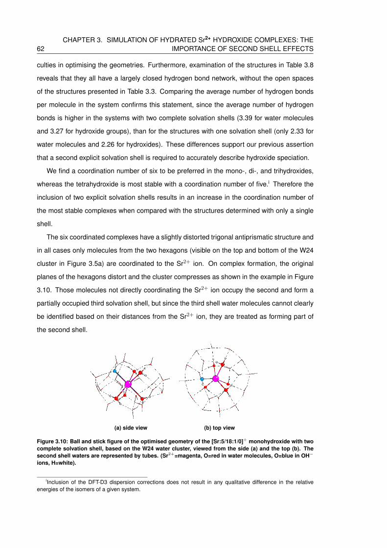
62CHAPTER 3. SIMULATION OF HYDRATED Sr2+ HYDROXIDE COMPLEXES: THE
IMPORTANCE OF SECOND SHELL EFFECTS
culties in optimising the geometries. Furthermore, examination of the structures in Table 3.8
reveals that they all have a largely closed hydrogen bond network, without the open spaces
of the structures presented in Table 3.3. Comparing the average number of hydrogen bonds
per molecule in the system confirms this statement, since the average number of hydrogen
bonds is higher in the systems with two complete solvation shells (3.39 for water molecules
and 3.27 for hydroxide groups), than for the structures with one solvation shell (only 2.33 for
water molecules and 2.26 for hydroxides). These differences support our previous assertion
that a second explicit solvation shell is required to accurately describe hydroxide speciation.
We find a coordination number of six to be preferred in the mono-, di-, and trihydroxides,
whereas the tetrahydroxide is most stable with a coordination number of five.i Therefore the
inclusion of two explicit solvation shells results in an increase in the coordination number of
the most stable complexes when compared with the structures determined with only a single
shell.
The six coordinated complexes have a slightly distorted trigonal antiprismatic structure and
in all cases only molecules from the two hexagons (visible on the top and bottom of the W24
cluster in Figure 3.5a) are coordinated to the Sr2+ ion. On complex formation, the original
planes of the hexagons distort and the cluster compresses as shown in the example in Figure
3.10. Those molecules not directly coordinating the Sr2+ ion occupy the second and form a
partially occupied third solvation shell, but since the third shell water molecules cannot clearly
be identified based on their distances from the Sr2+ ion, they are treated as forming part of
the second shell.
(a) side view (b) top view
Figure 3.10: Ball and stick figure of the optimised geometry of the [Sr:5/18:1/0]+ monohydroxide with twocomplete solvation shell, based on the W24 water cluster, viewed from the side (a) and the top (b). Thesecond shell waters are represented by tubes. (Sr2+=magenta, O=red in water molecules, O=blue in OH−
ions, H=white).
iInclusion of the DFT-D3 dispersion corrections does not result in any qualitative difference in the relativeenergies of the isomers of a given system.

3.4. RESULTS 63
The average Sr-O distances for the Sr2+ hydroxides and hydrates with a complete second
shell are summarised in Table 3.9. The average Sr-Ow distance in the first shell of the hydrate
complexes varies from 2.570[158] to 2.643 A[157] in previous experimental studies, in very
good agreement with our calculated bond length (2.616 A). With more hydroxide ions in the
system, the Sr-Ow distances of the first shell water molecules increase; it was previously
noted that higher hydroxide coordination weakens these bonds.[122] It might be expected that
the increasing Sr-Ow distances would be accompanied by a reduction of the partial charge on
the metal, and the average Mulliken Sr charge does indeed decrease from +1.151 to +1.089,
+1.024 and +1.019 in the mono through tetra hydroxo systems. The Sr-OOH distances in
the first and second shells also increase, presumably for the same reason. Conversely, the
Sr-Ow distances to the second shell waters decrease, as the weakening of the Sr first shell
water bonds leads to a stronger bonding between the first and second shells. However, the
calculated average bond length for the hydrate complex (4.464 A) is still some way from the
experimentally determined 4.940 A[153]. It is even less than the Sr-Ow distance measured in
the solid crystal structure (4.78 A).[146] This may well be the effect of overestimated hydrogen
bond strength in the whole system, due to the incomplete description of the environment by
the COSMO model.
Table 3.9: The average Sr-Ow and Sr-OOH distances (A) in the first and second solvation shell for Sr2+
hydrates and each type of hydroxide. For simplicity, water molecules in the third shell are included in thesecond shell averages. Standard deviations (SD) are presented in parentheses
Sr-OOH Sr-Ow
first second first second
Average SD Average SD Average SD Average SD
hydrate - - - - 2.616 (0.037) 4.464 (0.333)hydrate[153] - - - - 2.640 - 4.940 -hydrate[146]ii - - - - 2.63 - 4.78 -hydrate[158] - - - - 2.57 - - -hydrate[157] - - - - 2.643 - - -
mono 2.455 (0.008) 3.818 (0.009) 2.621 (0.020) 4.409 (0.324)di 2.476 (0.027) 3.874 (0.101) 2.634 (0.027) 4.401 (0.342)tri 2.481 (0.028) 4.049 - 2.668 (0.027) 4.394 (0.376)tetra 2.482 (0.018) - - 2.708 - 4.397 (0.410)
3.4.2.1 Proton transfer between solvation shells
If we compare the geometries of the different type of hydroxides in a given column of
Table 3.8, we find that structures which have fewer OH− ions coordinated to the Sr2+ can
iRef [146] is an XRD result based on solid state crystal structure.

64CHAPTER 3. SIMULATION OF HYDRATED Sr2+ HYDROXIDE COMPLEXES: THE
IMPORTANCE OF SECOND SHELL EFFECTS
be derived directly from those with more coordinated hydroxides via a proton transfer from a
second shell water molecule to a first shell hydroxyl group. In addition, the energies of the
structures in a given column are close to one another. For example, the Gibbs free energies
of the systems with three hydroxide ions and 21 water molecules span less than 3 kJ/mol:
A room temperature Boltzmann distribution suggests that these structures may coexist in the
following proportions: 19%, 26% and 55% for mono-, tri- and dihydroxides respectively (Table
3.10). Such small energy differences can be rationalised by the fact that OH− ions are stronger
hydrogen bond acceptors and weaker hydrogen bond donors than water molecules.[175, 177]
Therefore, a system which contains a direct Sr2+-OH− interaction with the coordinated OH−
ion involved in two strong hydrogen bonds as a donor and one weak hydrogen bond as an
acceptor (e.g. [Sr:4/18:2/0]) is competitively close in energy to a system with a direct Sr2+-
H2O interaction and an uncoordinated OH− ion which forms 3 strong hydrogen bonds with its
oxygen atom while its hydrogen atom is directed away from the structure (e.g. [Sr:5/17:1/1]).
Table 3.10: Boltzmann distribution of differently coordinated Sr2+ hydroxide complexes calculated basedon the Gibbs free energies at room temperature
Hydroxidecoordination
System composition1 OH−/23 H2O 2 OH−/22 H2O 3 OH−/21 H2O 4 OH−/20 H2O
mono 100% 76% 19% -di - 24% 55% 1%tri - - 26% 51%
tetra - - - 48%
A tendency for one hydroxide ion to migrate from the first to the second solvation shell
was reported previously for gas phase Sr2+ hydroxide complexes with one complete solva-
tion shell[122, 142] but, to the best of our knowledge, proton transfer between shells has not
been previously studied in the aqueous phase. We therefore sought the transition state for the
Sr2+ dihydroxide ([Sr:4/18:2/0]) −→ Sr2+ monohydroxide ([Sr:5/17:1/1]) reaction. The transi-
tion state was obtained by first exploring the energy profile along the H(H2O)-O(OH) reaction
coordinate, then carrying out a transition search at the H-O distance of the maximum of the
energy profile. The optimised transition state had one negative frequency in the vibrational
spectrum related to studied O-H stretching. The results are summarised in Table 3.11 and the
energy profile plotted in Figure 3.11, from which we can see that the Gibbs free energy barrier
for this reaction is very small (3.0 kJ/mol). Thus, the coordination can easily interchange be-
tween di- and monohydroxide in this system, suggesting that our explicit two shell model well
reflects the dynamical nature of the solutions, i.e. the frequent exchange of solvent molecules

3.4. RESULTS 65
and anions between the ion solvation shells and the bulk solvent.[198, 199]
Figure 3.11: Free energy profile (∆G) of proton transfer between the most stable dihydroxide ([Sr:4/18:2/0])and monohydroxide ([Sr:5/17:1/1]) complexes with 22 water molecules, from the second column of Table3.8. TS = transition state.
Table 3.11: SCF (∆ESCF) and Gibbs free energy differences (∆G) of the dihydroxide −→ monohydroxideproton transfer reaction. TS = transition state
(ESCF) (a.u.) ∆ESCF (kJ/mol) (SCF+Gcorr) (a.u.) ∆G (kJ/mol)
di [Sr:4/18:2/0] -1865.326957 0.0 -1864.851310 0.0TS -1865.326349 1.6 -1864.850185 3.0
mono [Sr:5/17:1/1] -1865.328093 -3.0 -1864.852268 -2.5
To rule out the possibility that the calculated small energy difference is a result of moving
a negative charge closer to the cavity, we compared the charges of every oxygen atom in the
complexes by QTAIM analysis. Although there is a slight difference between the charge of the
moving OH− ion between the two complex (OH2 changes from -1.274 to -1.210 in Table 3.12),
it seems that the Sr-O distance is responsible for this change as the first shell oxygen atoms
have a more negative charge in general than the second shell O atoms due to the polarising
effect of the cation (average -1.26 compared to -1.18) and the -2 charge carried by two OH−
ions seems almost evenly distributed between the O atoms of the complex, i.e. the charges
of oxygen atoms within the hydroxide ions are close to the average charge calculated for the
solvation shell in which they are (e.g. OH1 is -1.269 and -1.271 while the average charge of
oxygen atoms in the first solvation shell is 1.26). These results show no evidence of unrealistic
charges and artificial charge distribution to the vicinity of the cavity, therefore we can conclude
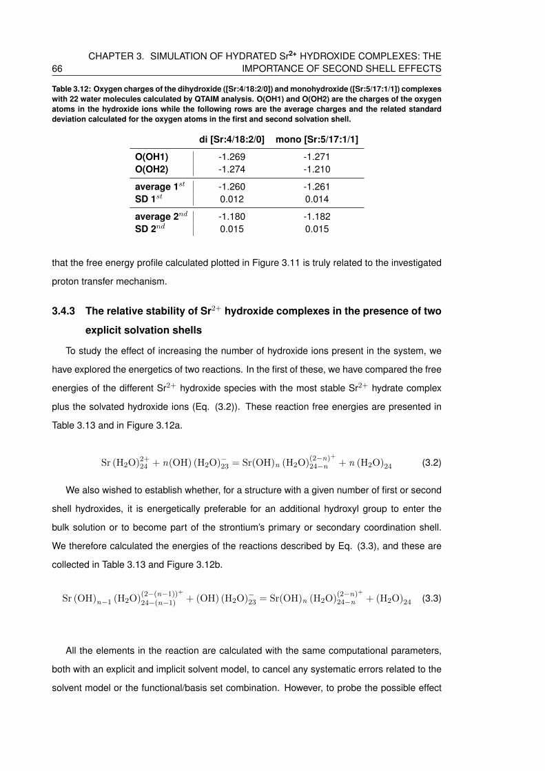
66CHAPTER 3. SIMULATION OF HYDRATED Sr2+ HYDROXIDE COMPLEXES: THE
IMPORTANCE OF SECOND SHELL EFFECTS
Table 3.12: Oxygen charges of the dihydroxide ([Sr:4/18:2/0]) and monohydroxide ([Sr:5/17:1/1]) complexeswith 22 water molecules calculated by QTAIM analysis. O(OH1) and O(OH2) are the charges of the oxygenatoms in the hydroxide ions while the following rows are the average charges and the related standarddeviation calculated for the oxygen atoms in the first and second solvation shell.
di [Sr:4/18:2/0] mono [Sr:5/17:1/1]
O(OH1) -1.269 -1.271O(OH2) -1.274 -1.210
average 1st -1.260 -1.261SD 1st 0.012 0.014
average 2nd -1.180 -1.182SD 2nd 0.015 0.015
that the free energy profile calculated plotted in Figure 3.11 is truly related to the investigated
proton transfer mechanism.
3.4.3 The relative stability of Sr2+ hydroxide complexes in the presence of two
explicit solvation shells
To study the effect of increasing the number of hydroxide ions present in the system, we
have explored the energetics of two reactions. In the first of these, we have compared the free
energies of the different Sr2+ hydroxide species with the most stable Sr2+ hydrate complex
plus the solvated hydroxide ions (Eq. (3.2)). These reaction free energies are presented in
Table 3.13 and in Figure 3.12a.
Sr (H2O)2+24 + n(OH) (H2O)−23 = Sr(OH)n (H2O)
(2−n)+
24−n + n (H2O)24 (3.2)
We also wished to establish whether, for a structure with a given number of first or second
shell hydroxides, it is energetically preferable for an additional hydroxyl group to enter the
bulk solution or to become part of the strontium’s primary or secondary coordination shell.
We therefore calculated the energies of the reactions described by Eq. (3.3), and these are
collected in Table 3.13 and Figure 3.12b.
Sr (OH)n−1 (H2O)(2−(n−1))+
24−(n−1) + (OH) (H2O)−23 = Sr(OH)n (H2O)(2−n)+
24−n + (H2O)24 (3.3)
All the elements in the reaction are calculated with the same computational parameters,
both with an explicit and implicit solvent model, to cancel any systematic errors related to the
solvent model or the functional/basis set combination. However, to probe the possible effect
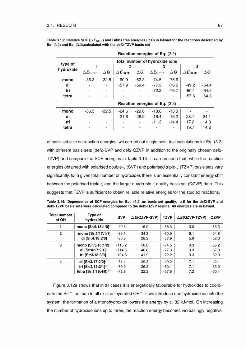
3.4. RESULTS 67
Table 3.13: Relative SCF (∆ESCF) and Gibbs free energies (∆G) in kJ/mol for the reactions described byEq. (3.2) and Eq. (3.3),calculated with the def2-TZVP basis set
Reaction energies of Eq. (3.2)
type ofhydroxide
total number of hydroxide ions1 2 3 4
∆ESCF ∆G ∆ESCF ∆G ∆ESCF ∆G ∆ESCF ∆G
mono -36.3 -32.5 -60.9 -62.3 -74.5 -75.6 - -di - - -57.9 -59.4 -77.3 -78.5 -49.2 -54.4tri - - - - -72.2 -76.7 -60.1 -64.5
tetra - - - - - - -57.6 -64.3
Reaction energies of Eq. (3.3)
mono -36.3 -32.5 -24.6 -29.8 -13.6 -13.3 - -di - - -21.6 -26.9 -16.4 -16.2 28.1 24.1tri - - - - -11.3 -14.4 17.2 14.0
tetra - - - - - - 19.7 14.2
of basis set size on reaction energies, we carried out single point test calculations for Eq. (3.2)
with different basis sets (def2-SVP and def2-QZVP in addition to the originally chosen def2-
TZVP) and compare the SCF energies in Table 3.14. It can be seen that, while the reaction
energies obtained with polarised double-ζ (SVP) and polarised triple-ζ (TZVP) basis sets vary
significantly, for a given total number of hydroxides there is an essentially constant energy shift
between the polarised triple-ζ and the larger quadruple-ζ quality basis set (QZVP) data. This
suggests that TZVP is sufficient to obtain reliable relative energies for the studied reactions.
Table 3.14: Dependence of SCF energies for Eq. (3.2) on basis set quality. ∆E for the def2-SVP anddef2-TZVP basis sets were calculated compared to the def2-QZVP results. All energies are in kJ/mol.
Total numberof OH
Type ofhydroxide
SVP ∆E(QZVP-SVP) TZVP ∆E(QZVP-TZVP) QZVP
1 mono [Sr:5/18:1/0]+ -49.3 16.0 -36.3 3.0 -33.3
2 mono [Sr:5/17:1/1] -89.1 34.3 -60.9 6.1 -54.8di [Sr:4/18:2/0] -80.3 28.2 -57.9 5.9 -52.0
3 mono [Sr:5/16:1/2]− -115.2 50.0 -74.5 9.3 -65.2di [Sr:4/17:2/1]− -114.6 46.6 -77.3 9.3 -67.9tri [Sr:3/18:3/0]− -104.8 41.9 -72.2 9.3 -62.9
4 di [Sr:3/17:2/2]2− -71.4 29.3 -49.2 7.1 -42.1tri [Sr:2/18:3/1]2− -79.2 26.2 -60.1 7.1 -53.0
tetra [Sr:1/19:4/0]2− -72.6 22.2 -57.6 7.2 -50.4
Figure 3.12a shows that in all cases it is energetically favourable for hydroxides to coordi-
nate the Sr2+ ion than to all exist as hydrated OH−. If we introduce one hydroxide ion into the
system, the formation of a monohydroxide lowers the energy by c. 32 kJ/mol. On increasing
the number of hydroxide ions up to three, the reaction energy becomes increasingly negative,
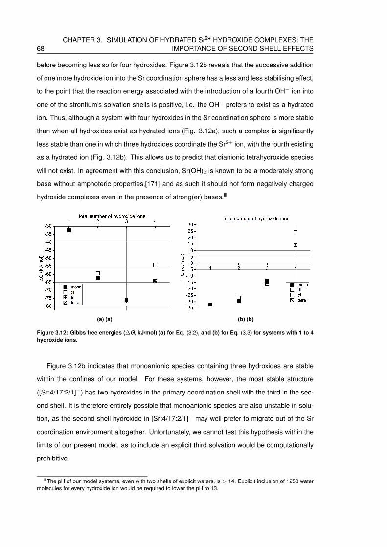
68CHAPTER 3. SIMULATION OF HYDRATED Sr2+ HYDROXIDE COMPLEXES: THE
IMPORTANCE OF SECOND SHELL EFFECTS
before becoming less so for four hydroxides. Figure 3.12b reveals that the successive addition
of one more hydroxide ion into the Sr coordination sphere has a less and less stabilising effect,
to the point that the reaction energy associated with the introduction of a fourth OH− ion into
one of the strontium’s solvation shells is positive, i.e. the OH− prefers to exist as a hydrated
ion. Thus, although a system with four hydroxides in the Sr coordination sphere is more stable
than when all hydroxides exist as hydrated ions (Fig. 3.12a), such a complex is significantly
less stable than one in which three hydroxides coordinate the Sr2+ ion, with the fourth existing
as a hydrated ion (Fig. 3.12b). This allows us to predict that dianionic tetrahydroxide species
will not exist. In agreement with this conclusion, Sr(OH)2 is known to be a moderately strong
base without amphoteric properties,[171] and as such it should not form negatively charged
hydroxide complexes even in the presence of strong(er) bases.iii
(a) (a) (b) (b)
Figure 3.12: Gibbs free energies (∆G, kJ/mol) (a) for Eq. (3.2), and (b) for Eq. (3.3) for systems with 1 to 4hydroxide ions.
Figure 3.12b indicates that monoanionic species containing three hydroxides are stable
within the confines of our model. For these systems, however, the most stable structure
([Sr:4/17:2/1]−) has two hydroxides in the primary coordination shell with the third in the sec-
ond shell. It is therefore entirely possible that monoanionic species are also unstable in solu-
tion, as the second shell hydroxide in [Sr:4/17:2/1]− may well prefer to migrate out of the Sr
coordination environment altogether. Unfortunately, we cannot test this hypothesis within the
limits of our present model, as to include an explicit third solvation would be computationally
prohibitive.
iiiThe pH of our model systems, even with two shells of explicit waters, is > 14. Explicit inclusion of 1250 watermolecules for every hydroxide ion would be required to lower the pH to 13.
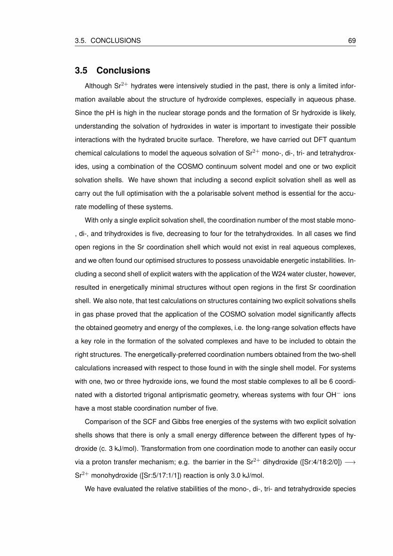
3.5. CONCLUSIONS 69
3.5 Conclusions
Although Sr2+ hydrates were intensively studied in the past, there is only a limited infor-
mation available about the structure of hydroxide complexes, especially in aqueous phase.
Since the pH is high in the nuclear storage ponds and the formation of Sr hydroxide is likely,
understanding the solvation of hydroxides in water is important to investigate their possible
interactions with the hydrated brucite surface. Therefore, we have carried out DFT quantum
chemical calculations to model the aqueous solvation of Sr2+ mono-, di-, tri- and tetrahydrox-
ides, using a combination of the COSMO continuum solvent model and one or two explicit
solvation shells. We have shown that including a second explicit solvation shell as well as
carry out the full optimisation with the a polarisable solvent method is essential for the accu-
rate modelling of these systems.
With only a single explicit solvation shell, the coordination number of the most stable mono-
, di-, and trihydroxides is five, decreasing to four for the tetrahydroxides. In all cases we find
open regions in the Sr coordination shell which would not exist in real aqueous complexes,
and we often found our optimised structures to possess unavoidable energetic instabilities. In-
cluding a second shell of explicit waters with the application of the W24 water cluster, however,
resulted in energetically minimal structures without open regions in the first Sr coordination
shell. We also note, that test calculations on structures containing two explicit solvations shells
in gas phase proved that the application of the COSMO solvation model significantly affects
the obtained geometry and energy of the complexes, i.e. the long-range solvation effects have
a key role in the formation of the solvated complexes and have to be included to obtain the
right structures. The energetically-preferred coordination numbers obtained from the two-shell
calculations increased with respect to those found in with the single shell model. For systems
with one, two or three hydroxide ions, we found the most stable complexes to all be 6 coordi-
nated with a distorted trigonal antiprismatic geometry, whereas systems with four OH− ions
have a most stable coordination number of five.
Comparison of the SCF and Gibbs free energies of the systems with two explicit solvation
shells shows that there is only a small energy difference between the different types of hy-
droxide (c. 3 kJ/mol). Transformation from one coordination mode to another can easily occur
via a proton transfer mechanism; e.g. the barrier in the Sr2+ dihydroxide ([Sr:4/18:2/0]) −→
Sr2+ monohydroxide ([Sr:5/17:1/1]) reaction is only 3.0 kJ/mol.
We have evaluated the relative stabilities of the mono-, di-, tri- and tetrahydroxide species

70CHAPTER 3. SIMULATION OF HYDRATED Sr2+ HYDROXIDE COMPLEXES: THE
IMPORTANCE OF SECOND SHELL EFFECTS
by calculating the energies of two reactions (defined by equations (3.2) and (3.3)). We found
that in all cases the Sr2+ hydroxide complexes are more stable than a Sr2+ hydrate plus
hydrated OH− ions. However, the addition of more hydroxide ions has a systematically weaker
stabilising effect, terminating at the point when adding a fourth OH− ion to the trihydroxide
species is energetically unfavourable. Furthermore, the most stable trihydroxide structure has
only two hydroxides in the first coordination shell of the Sr2+ ion, and we suggest that the
third hydroxide ligand may migrate away from the Sr coordination environment altogether if
our model contained a significantly larger number of explicit water molecules.
We conclude that the most likely Sr-hydroxide complexes to be found in high pH aqueous
solutions are mono- and dihydroxides, and that they coexist. These species are therefore the
most likely candidates for adsorption onto brucite surfaces under the pH conditions found in
fuel storage ponds, and can be used as reference systems for the Sr2+ ion’s behaviour in
the bulk solution. In the next chapter, I focus on the simulation of brucite (0001); describe the
development of the periodic electrostatic embedded cluster surface model and its validation by
simple adsorption studies in gas phase. While in the final result chapter the main conclusions
of this study (such as the necessary combination of an implicit solvent model with sufficient
number of explicit water molecules and the obtained structures of the most stable Sr2+ hydrate
and hydroxide complexes) are utilised for the investigation of Sr2+ adsorption on hydrated
brucite surfaces, bringing together the results of the present chapter and the following one.

Chapter 4
Modelling the (0001) brucite surface with the periodic
electrostatic embedded cluster method
4.1 Introduction
Developing a suitable surface representation for the (0001) brucite surface, which then can
be used to study the adsorption of solvated ions, is a crucial part of the research project,
as it has been shown that brucite is the most significant component of corroded Magnox
sludge and is capable of adsorbing some of the existing radioactive ions in the nuclear storage
ponds (see section 1.1). In this chapter, density functional theory at the meta-GGA level is
employed within the periodic electrostatic embedded cluster method (PEECM, 2.6.2) to model
the brucite (0001) surface. Representative studies are then used to demonstrate the reliability
of the PEECM for the description of the interactions of various ionic species with the layered
Mg(OH)2 structure, and its performance is compared with periodic DFT.
4.2 Literature review
This literature review is a detailed introduction to brucite: summarising the structural prop-
erties of the mineral, continued by the results of previous electronic structure calculations
and bond analysis and the introduction of brucite surfaces. It is followed by a comparison of
theoretical approaches used to study ionic adsorption.
4.2.1 The structure of the mineral brucite
Brucite is a layered mineral, containing Mg(OH)2 layers, in which the hydroxyl groups are
orthogonal to the hexagonal basal plane, see Figure 4.1 (space group is D33d, P3m1). The
following parameters describe completely the structure: a and c lattice parameters and zO, zH
atomic fractional coordinates (or alternatively the calculated internal coordinates, such as the
Mg-O, O-H bond and H· · ·H inter- and O· · ·O intralayer distance).[200, 201]
Three neutron diffraction studies have been used to compare the calculated geometrical
properties of different computational methods to experimental measurements in ambient con-
ditions: the first was published by Zigan and Rothbauer in 1967[203] the second one was a
high pressure study by Catti et al.[204] in which they measured the properties of brucite under
71
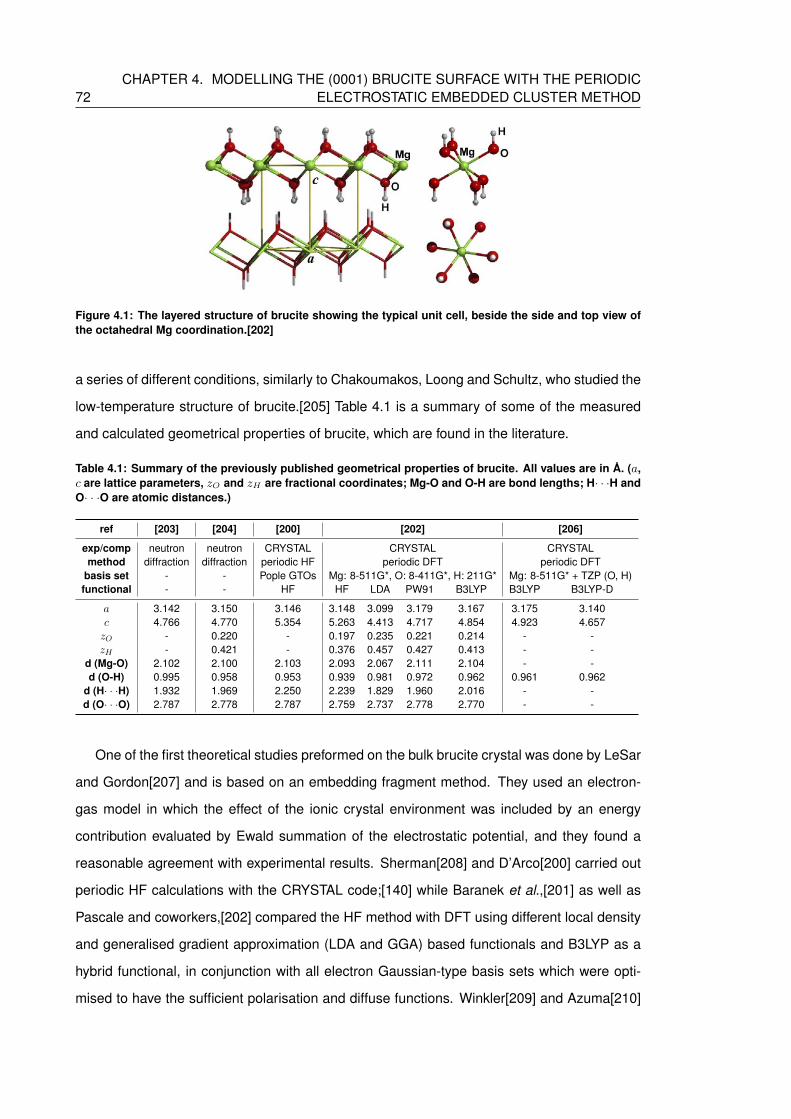
72CHAPTER 4. MODELLING THE (0001) BRUCITE SURFACE WITH THE PERIODIC
ELECTROSTATIC EMBEDDED CLUSTER METHOD
Figure 4.1: The layered structure of brucite showing the typical unit cell, beside the side and top view ofthe octahedral Mg coordination.[202]
a series of different conditions, similarly to Chakoumakos, Loong and Schultz, who studied the
low-temperature structure of brucite.[205] Table 4.1 is a summary of some of the measured
and calculated geometrical properties of brucite, which are found in the literature.
Table 4.1: Summary of the previously published geometrical properties of brucite. All values are in A. (a,c are lattice parameters, zO and zH are fractional coordinates; Mg-O and O-H are bond lengths; H· · ·H andO· · ·O are atomic distances.)
ref [203] [204] [200] [202] [206]
exp/comp neutron neutron CRYSTAL CRYSTAL CRYSTALmethod diffraction diffraction periodic HF periodic DFT periodic DFT
basis set - - Pople GTOs Mg: 8-511G*, O: 8-411G*, H: 211G* Mg: 8-511G* + TZP (O, H)functional - - HF HF LDA PW91 B3LYP B3LYP B3LYP-D
a 3.142 3.150 3.146 3.148 3.099 3.179 3.167 3.175 3.140c 4.766 4.770 5.354 5.263 4.413 4.717 4.854 4.923 4.657zO - 0.220 - 0.197 0.235 0.221 0.214 - -zH - 0.421 - 0.376 0.457 0.427 0.413 - -
d (Mg-O) 2.102 2.100 2.103 2.093 2.067 2.111 2.104 - -d (O-H) 0.995 0.958 0.953 0.939 0.981 0.972 0.962 0.961 0.962
d (H· · ·H) 1.932 1.969 2.250 2.239 1.829 1.960 2.016 - -d (O· · ·O) 2.787 2.778 2.787 2.759 2.737 2.778 2.770 - -
One of the first theoretical studies preformed on the bulk brucite crystal was done by LeSar
and Gordon[207] and is based on an embedding fragment method. They used an electron-
gas model in which the effect of the ionic crystal environment was included by an energy
contribution evaluated by Ewald summation of the electrostatic potential, and they found a
reasonable agreement with experimental results. Sherman[208] and D’Arco[200] carried out
periodic HF calculations with the CRYSTAL code;[140] while Baranek et al.,[201] as well as
Pascale and coworkers,[202] compared the HF method with DFT using different local density
and generalised gradient approximation (LDA and GGA) based functionals and B3LYP as a
hybrid functional, in conjunction with all electron Gaussian-type basis sets which were opti-
mised to have the sufficient polarisation and diffuse functions. Winkler[209] and Azuma[210]
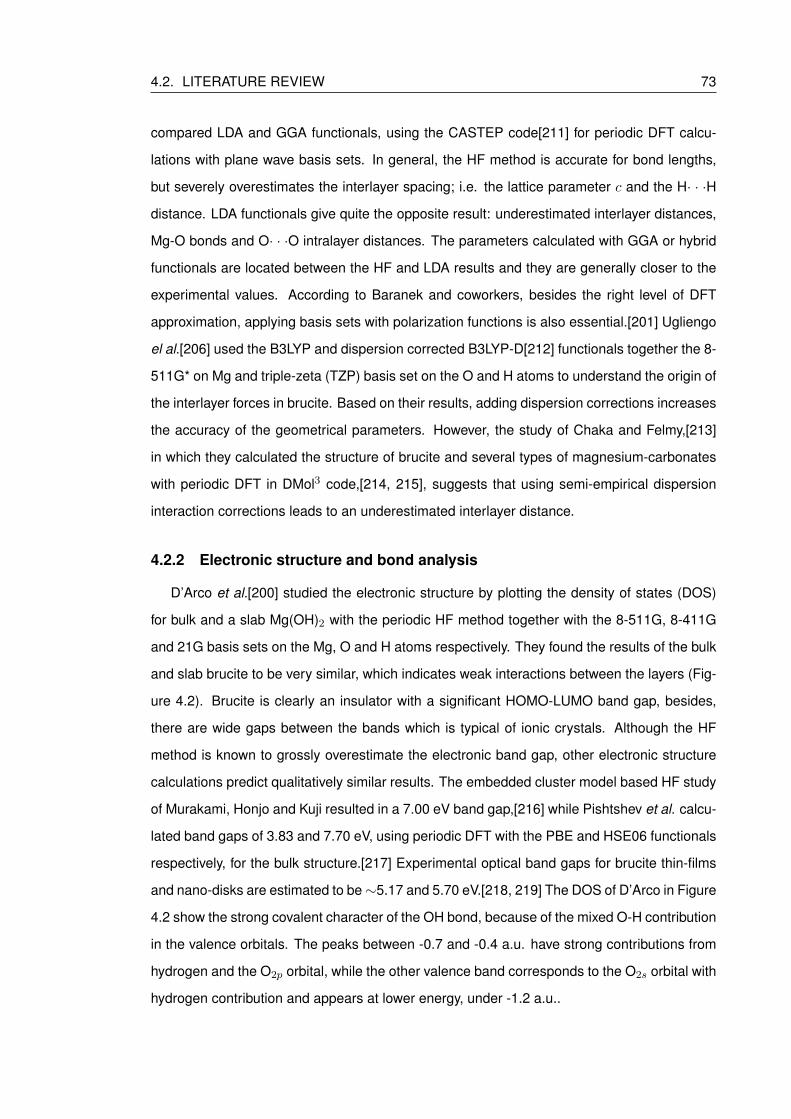
4.2. LITERATURE REVIEW 73
compared LDA and GGA functionals, using the CASTEP code[211] for periodic DFT calcu-
lations with plane wave basis sets. In general, the HF method is accurate for bond lengths,
but severely overestimates the interlayer spacing; i.e. the lattice parameter c and the H· · ·H
distance. LDA functionals give quite the opposite result: underestimated interlayer distances,
Mg-O bonds and O· · ·O intralayer distances. The parameters calculated with GGA or hybrid
functionals are located between the HF and LDA results and they are generally closer to the
experimental values. According to Baranek and coworkers, besides the right level of DFT
approximation, applying basis sets with polarization functions is also essential.[201] Ugliengo
el al.[206] used the B3LYP and dispersion corrected B3LYP-D[212] functionals together the 8-
511G* on Mg and triple-zeta (TZP) basis set on the O and H atoms to understand the origin of
the interlayer forces in brucite. Based on their results, adding dispersion corrections increases
the accuracy of the geometrical parameters. However, the study of Chaka and Felmy,[213]
in which they calculated the structure of brucite and several types of magnesium-carbonates
with periodic DFT in DMol3 code,[214, 215], suggests that using semi-empirical dispersion
interaction corrections leads to an underestimated interlayer distance.
4.2.2 Electronic structure and bond analysis
D’Arco et al.[200] studied the electronic structure by plotting the density of states (DOS)
for bulk and a slab Mg(OH)2 with the periodic HF method together with the 8-511G, 8-411G
and 21G basis sets on the Mg, O and H atoms respectively. They found the results of the bulk
and slab brucite to be very similar, which indicates weak interactions between the layers (Fig-
ure 4.2). Brucite is clearly an insulator with a significant HOMO-LUMO band gap, besides,
there are wide gaps between the bands which is typical of ionic crystals. Although the HF
method is known to grossly overestimate the electronic band gap, other electronic structure
calculations predict qualitatively similar results. The embedded cluster model based HF study
of Murakami, Honjo and Kuji resulted in a 7.00 eV band gap,[216] while Pishtshev et al. calcu-
lated band gaps of 3.83 and 7.70 eV, using periodic DFT with the PBE and HSE06 functionals
respectively, for the bulk structure.[217] Experimental optical band gaps for brucite thin-films
and nano-disks are estimated to be∼5.17 and 5.70 eV.[218, 219] The DOS of D’Arco in Figure
4.2 show the strong covalent character of the OH bond, because of the mixed O-H contribution
in the valence orbitals. The peaks between -0.7 and -0.4 a.u. have strong contributions from
hydrogen and the O2p orbital, while the other valence band corresponds to the O2s orbital with
hydrogen contribution and appears at lower energy, under -1.2 a.u..
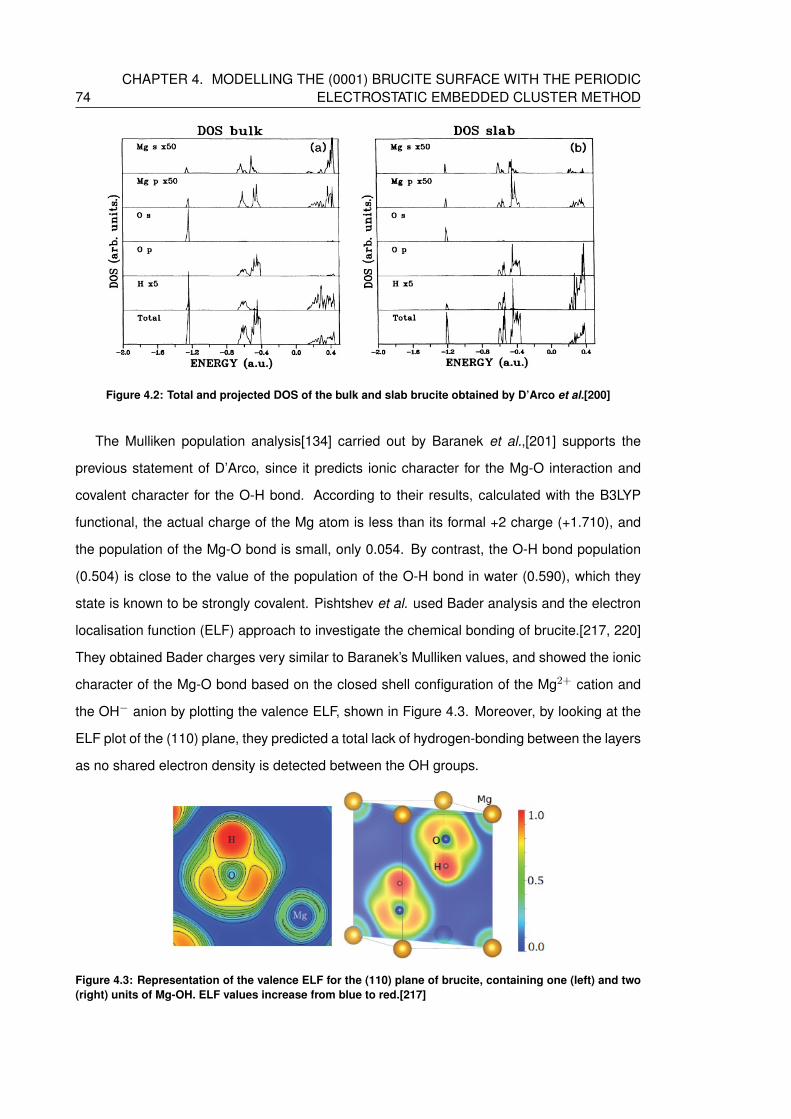
74CHAPTER 4. MODELLING THE (0001) BRUCITE SURFACE WITH THE PERIODIC
ELECTROSTATIC EMBEDDED CLUSTER METHOD
Figure 4.2: Total and projected DOS of the bulk and slab brucite obtained by D’Arco et al.[200]
The Mulliken population analysis[134] carried out by Baranek et al.,[201] supports the
previous statement of D’Arco, since it predicts ionic character for the Mg-O interaction and
covalent character for the O-H bond. According to their results, calculated with the B3LYP
functional, the actual charge of the Mg atom is less than its formal +2 charge (+1.710), and
the population of the Mg-O bond is small, only 0.054. By contrast, the O-H bond population
(0.504) is close to the value of the population of the O-H bond in water (0.590), which they
state is known to be strongly covalent. Pishtshev et al. used Bader analysis and the electron
localisation function (ELF) approach to investigate the chemical bonding of brucite.[217, 220]
They obtained Bader charges very similar to Baranek’s Mulliken values, and showed the ionic
character of the Mg-O bond based on the closed shell configuration of the Mg2+ cation and
the OH− anion by plotting the valence ELF, shown in Figure 4.3. Moreover, by looking at the
ELF plot of the (110) plane, they predicted a total lack of hydrogen-bonding between the layers
as no shared electron density is detected between the OH groups.
Figure 4.3: Representation of the valence ELF for the (110) plane of brucite, containing one (left) and two(right) units of Mg-OH. ELF values increase from blue to red.[217]
4.2. LITERATURE REVIEW 75
4.2.3 Interlayer forces in brucite
All the previous studies agree that the interlayer interactions are weak, but the nature of
these interactions is not completely clear. A minority of the studies suggest some hydrogen-
bonding between the layers, for example Kruger et al., based on vibrational spectrum analysis
done at various pressures, state that hydrogen-bonds are present in brucite even at high vac-
uum.[221] Haycock also assumed hydrogen-bonding during the analysis of his X-ray emission,
X-ray photoelectron and Auger spectroscopy results.[222] But the majority of the studies pre-
dict only dispersion type forces between the brucite layers. For instance, Bernal and Megaw
suggested a lack of hydrogen-bonding, based on the long O· · ·O intralayer distances in the
structure.[223] While Chaka and Felmy explain the lack of hydrogen-bonding in terms of the
coordination of the oxygen atoms: as all O atoms are coordinated to three Mg atoms and
bonded to one hydrogen, there is no electron lone pair left for the hydrogen bonding.[213]
The O-H stretching frequency is a good indicator of hydrogen-bonding, since its value
reflects the properties of the environment of the bond and therefore it is often evaluated in
computational studies.[210] Based on the factor group analysis, there is a Raman-active OH
stretch with A1g symmetry and an IR-active A2u,[221] which both have high frequencies (Ra-
man: ∼3655 cm−1 and IR ∼3700 cm−1)[221, 224–227] suggesting that the protons are not
involved in hydrogen-bonding.[209] However, according to Pascale et al., due to significant
interlayer couplings, there are some differences in the translational modes between the calcu-
lated spectra of the bulk structure and the spectra of a single layer of brucite.[202]
Many of the previous studies contain calculations of the interlayer forces. The so called
interlayer interaction energy (IE) is the energy difference between the optimised bulk structure
and the energy of isolated two dimensional layers,[210] i.e. larger IE values correspond to
stronger interlayer interaction. Some of the previously published results are summarised in
Table 4.2. Neglecting the dispersion forces in the calculations can lead to artificially weak
interaction and therefore an overestimated interlayer distance, as shown in the case of the HF
calculations. LDA functionals predict an overly strong interaction which leads to a severely
underestimated distance. GGA or hybrid functionals give interaction energies between the HF
and LDA results, but still underestimate the strength of the attraction, according to Ugliengo
et al.[206] They found that using a functional with dispersion corrections, such as B3LYP-
D instead of B3LYP, may improve the accuracy of the calculations (structural optimisation
and frequency) and give a much higher interaction energy (-22 kJ/mol instead of -3.8 kJ/mol,
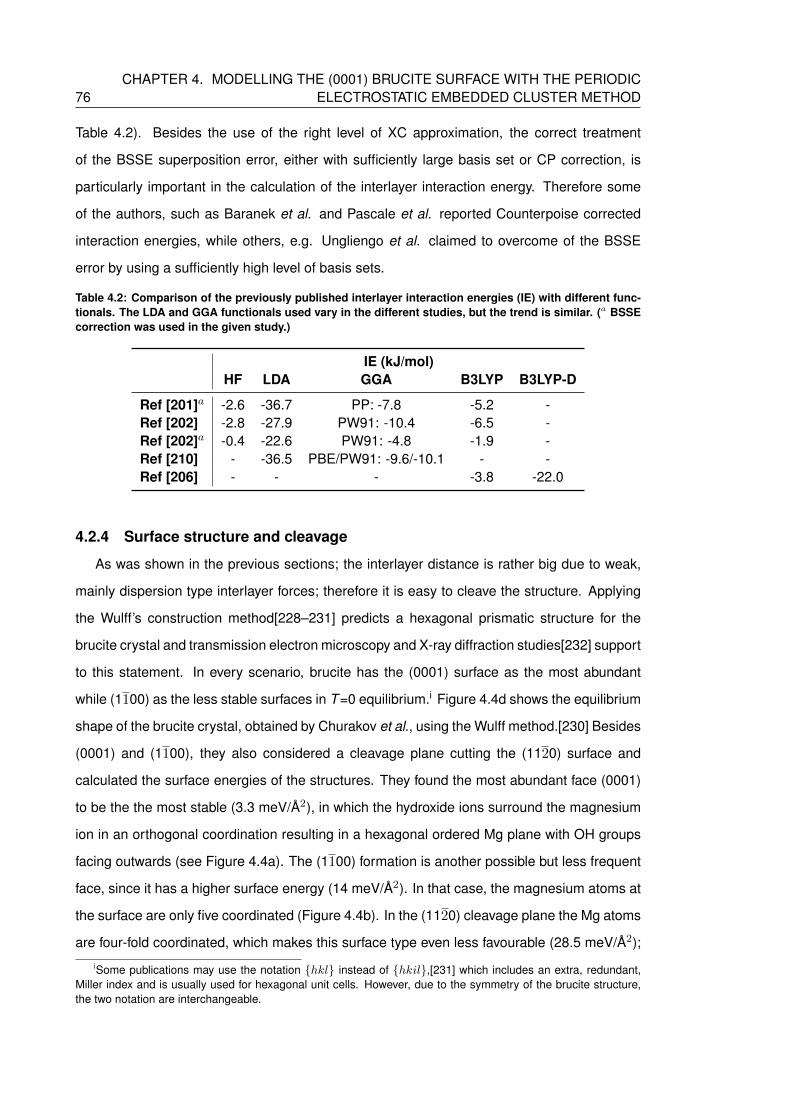
76CHAPTER 4. MODELLING THE (0001) BRUCITE SURFACE WITH THE PERIODIC
ELECTROSTATIC EMBEDDED CLUSTER METHOD
Table 4.2). Besides the use of the right level of XC approximation, the correct treatment
of the BSSE superposition error, either with sufficiently large basis set or CP correction, is
particularly important in the calculation of the interlayer interaction energy. Therefore some
of the authors, such as Baranek et al. and Pascale et al. reported Counterpoise corrected
interaction energies, while others, e.g. Ungliengo et al. claimed to overcome of the BSSE
error by using a sufficiently high level of basis sets.
Table 4.2: Comparison of the previously published interlayer interaction energies (IE) with different func-tionals. The LDA and GGA functionals used vary in the different studies, but the trend is similar. (a BSSEcorrection was used in the given study.)
IE (kJ/mol)HF LDA GGA B3LYP B3LYP-D
Ref [201]a -2.6 -36.7 PP: -7.8 -5.2 -Ref [202] -2.8 -27.9 PW91: -10.4 -6.5 -Ref [202]a -0.4 -22.6 PW91: -4.8 -1.9 -Ref [210] - -36.5 PBE/PW91: -9.6/-10.1 - -Ref [206] - - - -3.8 -22.0
4.2.4 Surface structure and cleavage
As was shown in the previous sections; the interlayer distance is rather big due to weak,
mainly dispersion type interlayer forces; therefore it is easy to cleave the structure. Applying
the Wulff’s construction method[228–231] predicts a hexagonal prismatic structure for the
brucite crystal and transmission electron microscopy and X-ray diffraction studies[232] support
to this statement. In every scenario, brucite has the (0001) surface as the most abundant
while (1100) as the less stable surfaces in T=0 equilibrium.i Figure 4.4d shows the equilibrium
shape of the brucite crystal, obtained by Churakov et al., using the Wulff method.[230] Besides
(0001) and (1100), they also considered a cleavage plane cutting the (1120) surface and
calculated the surface energies of the structures. They found the most abundant face (0001)
to be the the most stable (3.3 meV/A2), in which the hydroxide ions surround the magnesium
ion in an orthogonal coordination resulting in a hexagonal ordered Mg plane with OH groups
facing outwards (see Figure 4.4a). The (1100) formation is another possible but less frequent
face, since it has a higher surface energy (14 meV/A2). In that case, the magnesium atoms at
the surface are only five coordinated (Figure 4.4b). In the (1120) cleavage plane the Mg atoms
are four-fold coordinated, which makes this surface type even less favourable (28.5 meV/A2);
iSome publications may use the notation hkl instead of hkil,[231] which includes an extra, redundant,Miller index and is usually used for hexagonal unit cells. However, due to the symmetry of the brucite structure,the two notation are interchangeable.

4.2. LITERATURE REVIEW 77
according to Masini and Bernasconi, it occurs only in metastable phases.[229] The latter two
faces both have hydroxyl groups rotating outwards from the surface plane to minimise the
electrostatic repulsion among them as shown in Figure 4.4b and 4.4c. Because of the less
coordinated Mg atoms, there are dangling bonds at the surface which cause changes in the
interlayer distances between the first few layers.[230]
Figure 4.4: Optimised structures of the possible cleavages of the brucite surface: (a) side view of the(0001) structure, (b) of the (1100) surface and (c) of the (1120) cleavage. The dotted lines indicate theatomic planes in the surface, while the numbers are interatomic distances in the relaxed surface. Relativechanges in the interatomic distances compared to the equilibrium bulk are shown in brackets. (d) is theequilibrium shape of the brucite crystal, obtained by the Wulf’s construction method.[230]
Since the most common surface type is (0001) and water adsorption occurs on this hy-
droxyl terminated cleavage plane, its properties are better known than the other surfaces.
Moreover, while the basal plane of brucite (0001) is generally well described by force field
parameters, the description of the (1100) surface properties is less developed in molecular
dynamics studies. As a consequence, the surface hydroxyl groups tend to distort in a non-
realistic way which results in impossible mineral edges. To prevent this, Zeitler et al.[233]
recently developed a modified force field to improve the accuracy of simulations involving
these type of edges. The description of the (1100) surface can be important for example in
dehydroxlation reactions, because, according to the CPMD study of Churakov et al.[230], it
can be dehydroxlated easier than other surfaces. Churakov also states that layers under the
top one in the slab does not take part in the studied reactions, therefore they can be fixed in

78CHAPTER 4. MODELLING THE (0001) BRUCITE SURFACE WITH THE PERIODIC
ELECTROSTATIC EMBEDDED CLUSTER METHOD
the calculations.
4.3 Modelling ionic adsorption on surfaces
Theoretical studies of physical and chemical interactions on surfaces play a key role in
the understanding and predicting of many industrially relevant phenomena, including the ones
related to nuclear waste, as demonstrated in section 1.4. However, choosing a suitable sur-
face representation for the investigation of a particular adsorption mechanism is not always
straightforward, and the choice can heavily influence the outcome of the results.
One of the most common approaches to model surfaces is periodic density functional the-
ory (DFT), which operates with conventional unit cells and employs periodic boundary condi-
tions (see 2.6.1). However, modelling charged systems using periodic boundary conditions is
extremely difficult and is often treated by using background charges[38, 234, 235] or including
counter ions in the simulation box.[38, 42] In principle, a non-neutral simulation box under
PBCs (periodic boundary conditions) would result in an infinite, self-interacting charge and
an infinitely large electrostatic energy.[108, 234, 235] Employing a compensating homoge-
neous background charge within the cell to have a finite energy will inevitably lead to artificial
Coulomb interactions between the charged species and the background charge, and will not
prevent the interaction of the charged species with their own periodic images, resulting in artifi-
cial components in the absolute energy of the system.[38] Weber et al. studied the adsorption
of ionic liquid components on anatase with the periodic DFT method (PBE-D3 and PBE0 func-
tional/GTH pseudopotential basis set), and showed that by using very large supercells (see
Figure 4.5), the ionic species can be isolated from the neighbouring interaction sites and the
background charge is ”diluted” enough to significantly decrease the magnitude of the artificial
effect,[38] but with the price of significantly increased computational cost and limitations on
the practicable size of the basis sets. Although the absolute energies of non-neutral systems
obtained via PBC methods may not be always reliable, the calculation of relative energies and
the comparison of different conformations is still possible upon the application of a background
charge or counter ions with a sufficiently large cell size.
One alternative to modelling a surface with periodic DFT is to use isolated molecular clus-
ters to represent the adsorption site of the surface. This approach has been used mainly for
2D materials, such as graphene,[41] where the far-field effects of the substrate on the adsorp-
tion reaction can be neglected, i.e. the interaction is very localised; or where the effect of
extended surfaces were deliberately neglected for the sake of simplification[236, 237]. How-
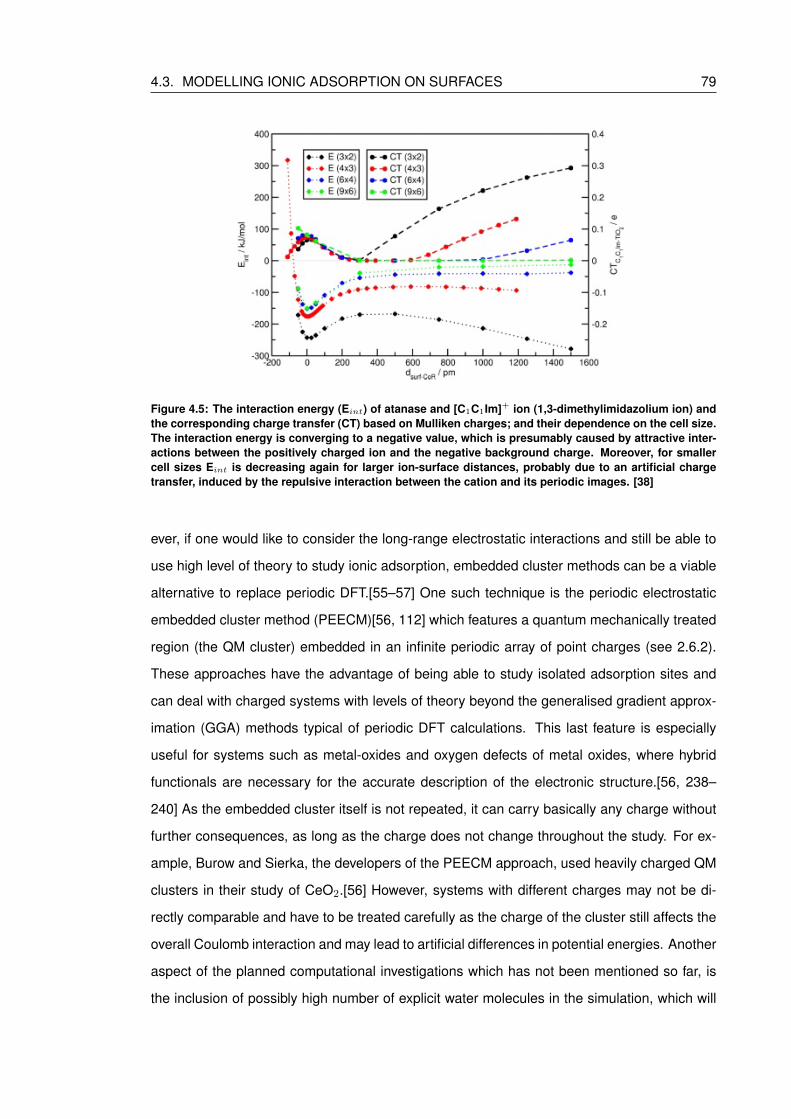
4.3. MODELLING IONIC ADSORPTION ON SURFACES 79
Figure 4.5: The interaction energy (Eint) of atanase and [C1C1Im]+ ion (1,3-dimethylimidazolium ion) andthe corresponding charge transfer (CT) based on Mulliken charges; and their dependence on the cell size.The interaction energy is converging to a negative value, which is presumably caused by attractive inter-actions between the positively charged ion and the negative background charge. Moreover, for smallercell sizes Eint is decreasing again for larger ion-surface distances, probably due to an artificial chargetransfer, induced by the repulsive interaction between the cation and its periodic images. [38]
ever, if one would like to consider the long-range electrostatic interactions and still be able to
use high level of theory to study ionic adsorption, embedded cluster methods can be a viable
alternative to replace periodic DFT.[55–57] One such technique is the periodic electrostatic
embedded cluster method (PEECM)[56, 112] which features a quantum mechanically treated
region (the QM cluster) embedded in an infinite periodic array of point charges (see 2.6.2).
These approaches have the advantage of being able to study isolated adsorption sites and
can deal with charged systems with levels of theory beyond the generalised gradient approx-
imation (GGA) methods typical of periodic DFT calculations. This last feature is especially
useful for systems such as metal-oxides and oxygen defects of metal oxides, where hybrid
functionals are necessary for the accurate description of the electronic structure.[56, 238–
240] As the embedded cluster itself is not repeated, it can carry basically any charge without
further consequences, as long as the charge does not change throughout the study. For ex-
ample, Burow and Sierka, the developers of the PEECM approach, used heavily charged QM
clusters in their study of CeO2.[56] However, systems with different charges may not be di-
rectly comparable and have to be treated carefully as the charge of the cluster still affects the
overall Coulomb interaction and may lead to artificial differences in potential energies. Another
aspect of the planned computational investigations which has not been mentioned so far, is
the inclusion of possibly high number of explicit water molecules in the simulation, which will

80CHAPTER 4. MODELLING THE (0001) BRUCITE SURFACE WITH THE PERIODIC
ELECTROSTATIC EMBEDDED CLUSTER METHOD
significantly increase the computational cost and determines our choice in modelling meth-
ods; as the computational performance of PEECM is much more efficient for systems with low
symmetry, than the periodic DFT methods.
After identifying the most stable hydroxide complexes of Sr2+ in aqueous solution in the
previous chapter, here we move on to develop an efficient model for studying the adsorp-
tion of Sr2+ complexes on the hydrated (0001) brucite surface. Based on the considerations
presented in the previous paragraphs, we decided to use the PEECM method, which has
previously been successfully employed to study ionic materials.[55, 56] As it was shown in
section 4.2.2; electronic structure calculations as well as Mulliken bond population analy-
sis[201] predict largely ionic character for the Mg-O bond but more covalent character for the
O-H bond. This feature of the material allows us to employ embedded methods, as we define
the QM cluster without cutting covalent bonds at the boundaries.[216] Although there are a
small number of examples for similar embedded calculations,[216, 241, 242] to the best of
our knowledge, this is the first time a surface of a not purely ionic material has been modelled
with the PEECM. The bulk of the results presented in this chapter was published in the follow-
ing paper: E. Makkos, A. Kerridge, J. Austin, N. Kaltsoyannis, Journal of Chemical Physics,
(2016) 145, 204708.[243]
4.4 Computational details
4.4.1 PEECM models
All calculations were performed with version 6.6 of the TURBOMOLE program[137] us-
ing resolution-of-the-identity density functional theory[180]. Results were visualised with the
MOLDRAW chemical graphical software.[184] The TPSS exchange-correlation functional,
which employs the meta-generalised gradient approximation (meta-GGA),[77] was used be-
cause it has been shown to describe Sr2+ complexes well in the past[149] and previous the-
oretical studies on brucite have shown that GGA functionals efficiently describe bulk proper-
ties.[201, 202, 209] Due to the large number of the quantum chemically treated atoms, the
def2-SVP basis sets of polarised double-ζ quality[87, 96] were used for all QM atoms. Partial
geometry optimisations, in which the boundary atoms of the cluster were held fixed and the
inner atoms allowed to fully relax (see Figure 4.6ii), were carried out in the gas phase, with the
m4 integration grid and the default convergence criteria: SCF energy: 10−6 a.u., structural
iiFor the 6x6 1+PC surface representation, the lower hydrogen atoms were also constrained during optimisa-tion.
4.4. COMPUTATIONAL DETAILS 81
energy: 10−6 a.u. and energy gradient: 10−3 a.u.
For every s block ion investigated in section 4.5.1 (Na+, Rb+, Cs+ and Mg2+, Sr2+, Ba2+),
the def2-SVP basis set[87, 94, 96] was used during the geometry optimisation along with the
associated effective core potentials[97] for Rb, Cs, Sr and Ba. The electron density distribu-
tion calculations reported in section 4.5.1 were performed by generating wavefunction (.wfn)
files from the output of the optimisation in TURBOMOLE using the molden2aim program[129]
which served as an input for the Multiwfn code[139]. The electron density images were plotted
with the VMD[244] visualisation code, using an isosurface value of 0.0025 a.u.
The Quantum Theory of Atoms in Molecules (QTAIM) calculations described in section
4.5.4 were performed with the professional version 13.11.04 of AIMAll[130] using the default
parameters of the program. The required .wfn files were generated as described above.
Considerations of the QM cluster
Due to its layered structure, the brucite surface was considered as a slab containing one
or more layers of Mg(OH)2 and modelled using the periodic electrostatic embedded cluster
method (PEECM, see section 2.6.2), implemented in the TURBOMOLE code. In this ap-
proach, a finite sized cluster of brucite was treated quantum chemically and embedded in a
2D infinite array of point charges (PCs) (aperiodic in the z direction). Experimental cell pa-
rameters, obtained via neutron diffraction measurements by Catti et al.,[204] were used to
define both the initial geometry for the QM cluster and the positions of the PCs in the infinite
two dimensional array: the a and b lattice parameters of the hexagonal unit cell were 3.15
A, and the interlayer distance c was 4.77 A. As it was described in section 4.2.3 and 4.2.4
the cleavage (0001) surface is the most stable brucite surface with a large interlayer distance
and weak interlayer forces, i.e. the structural changes during surface relaxation are negligi-
ble[200, 202, 229] and therefore the use of experimental bulk parameters for the fixed position
of boundary atoms and point charges should only introduce a negligible error in the obtained
surface structures.
The basic structure used for the investigations was a single layer of brucite containing
a stoichiometric 6x6 Mg atom QM cluster (Mg36(OH)72) embedded in the PCs, holding the
boundary atoms of the cluster fixed during the optimisation (shown in Figure 4.6). Building
on this geometry, several variations were proposed for the optimal surface representation, for
which we use the following notation from now on: ”nxn m”, where n is the number of Mg
atoms in the x and y direction and m is the number of brucite layers explicitly included in the
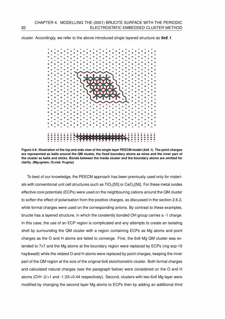
82CHAPTER 4. MODELLING THE (0001) BRUCITE SURFACE WITH THE PERIODIC
ELECTROSTATIC EMBEDDED CLUSTER METHOD
cluster. Accordingly, we refer to the above introduced single layered structure as 6x6 1.
Figure 4.6: Illustration of the top and side view of the single layer PEECM model (6x6 1). The point chargesare represented as balls around the QM cluster, the fixed boundary atoms as wires and the inner part ofthe cluster as balls and sticks. Bonds between the inside cluster and the boundary atoms are omitted forclarity. (Mg=green, O=red, H=grey)
To best of our knowledge, the PEECM approach has been previously used only for materi-
als with conventional unit cell structures such as TiO2[55] or CeO2[56]. For these metal oxides
effective core potentials (ECPs) were used on the neighbouring cations around the QM cluster
to soften the effect of polarisation from the positive charges, as discussed in the section 2.6.2,
while formal charges were used on the corresponding anions. By contrast to these examples,
brucite has a layered structure, in which the covalently bonded OH group carries a -1 charge.
In this case, the use of an ECP region is complicated and any attempts to create an isolating
shell by surrounding the QM cluster with a region containing ECPs as Mg atoms and point
charges as the O and H atoms are failed to converge. First, the 6x6 Mg QM cluster was ex-
tended to 7x7 and the Mg atoms at the boundary region were replaced by ECPs (mg ecp-10
hay&wadt) while the related O and H atoms were replaced by point charges, keeping the inner
part of the QM region at the size of the original 6x6 stoichiometric cluster. Both formal charges
and calculated natural charges (see the paragraph below) were considered on the O and H
atoms (O/H -2/+1 and -1.33/+0.44 respectively). Second, clusters with two 6x6 Mg layer were
modified by changing the second layer Mg atoms to ECPs then by adding an additional third
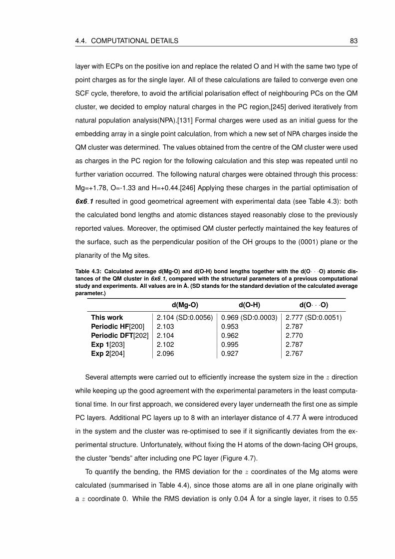
4.4. COMPUTATIONAL DETAILS 83
layer with ECPs on the positive ion and replace the related O and H with the same two type of
point charges as for the single layer. All of these calculations are failed to converge even one
SCF cycle, therefore, to avoid the artificial polarisation effect of neighbouring PCs on the QM
cluster, we decided to employ natural charges in the PC region,[245] derived iteratively from
natural population analysis(NPA).[131] Formal charges were used as an initial guess for the
embedding array in a single point calculation, from which a new set of NPA charges inside the
QM cluster was determined. The values obtained from the centre of the QM cluster were used
as charges in the PC region for the following calculation and this step was repeated until no
further variation occurred. The following natural charges were obtained through this process:
Mg=+1.78, O=-1.33 and H=+0.44.[246] Applying these charges in the partial optimisation of
6x6 1 resulted in good geometrical agreement with experimental data (see Table 4.3): both
the calculated bond lengths and atomic distances stayed reasonably close to the previously
reported values. Moreover, the optimised QM cluster perfectly maintained the key features of
the surface, such as the perpendicular position of the OH groups to the (0001) plane or the
planarity of the Mg sites.
Table 4.3: Calculated average d(Mg-O) and d(O-H) bond lengths together with the d(O· · ·O) atomic dis-tances of the QM cluster in 6x6 1, compared with the structural parameters of a previous computationalstudy and experiments. All values are in A. (SD stands for the standard deviation of the calculated averageparameter.)
d(Mg-O) d(O-H) d(O· · ·O)
This work 2.104 (SD:0.0056) 0.969 (SD:0.0003) 2.777 (SD:0.0051)Periodic HF[200] 2.103 0.953 2.787Periodic DFT[202] 2.104 0.962 2.770Exp 1[203] 2.102 0.995 2.787Exp 2[204] 2.096 0.927 2.767
Several attempts were carried out to efficiently increase the system size in the z direction
while keeping up the good agreement with the experimental parameters in the least computa-
tional time. In our first approach, we considered every layer underneath the first one as simple
PC layers. Additional PC layers up to 8 with an interlayer distance of 4.77 A were introduced
in the system and the cluster was re-optimised to see if it significantly deviates from the ex-
perimental structure. Unfortunately, without fixing the H atoms of the down-facing OH groups,
the cluster ”bends” after including one PC layer (Figure 4.7).
To quantify the bending, the RMS deviation for the z coordinates of the Mg atoms were
calculated (summarised in Table 4.4), since those atoms are all in one plane originally with
a z coordinate 0. While the RMS deviation is only 0.04 A for a single layer, it rises to 0.55

84CHAPTER 4. MODELLING THE (0001) BRUCITE SURFACE WITH THE PERIODIC
ELECTROSTATIC EMBEDDED CLUSTER METHOD
Figure 4.7: A side view of 6x6 Mg embedded brucite cluster (Mg36(OH)72) and one PC layer underneath.Atoms in the QM region are represented by wires, while the outer part by points. (Mg=green, O=red,H=grey)
A on introducing a PC layer. Besides, there is a decrement in the SCF energy due to the
electrostatic attraction of the first PC layer. Interestingly, after adding the first point charge
layer underneath, including extra layers has no effect on the SCF energies or RMS deviation
values, thus we did not pursue the addition of more than one PC layers further.
Table 4.4: SCF energies and the RMS deviation of the Mg z coordinates in the systems with a 6x6 Mg(OH)2cluster and 0 to 8 PC layers
total number of layers PC layers SCF energy (a.u.) RMS z (A)
1 0 -12666.68382 0.040
2 1 -12666.96102 0.5503 2 -12666.96103 0.5504 3 -12666.96103 0.5505 4 -12666.96103 0.5506 5 -12666.96104 0.5507 6 -12666.96104 0.5508 7 -12666.96104 0.5509 8 -12666.96104 0.550
To eliminate the overly strong attraction of the underlying point charges, we either decrease
the interlayer distance between the layers to create compensating repulsion forces between
the layers, modify the relative charges of the O and H centres further; or fix the positions of the
down-facing hydrogen atoms in the explicit cluster. We excluded the first solution because,
although attempts to decrease the interlayer distance from 4.77 A to 3.47 A in a system with
1 extra PC layer resulted in an RMS and energy minima below 4 Awith a RMS deviation 0.046
A (Figure 4.8), which is close to the single layer value; SCF convergence problems appeared
close to the energetic minimum. If we decreased the interlayer distance further, the explicit
cluster, in addition to convex deformation, deprotonated and was impossible to stabilise. We
also exluded the second approach, since it would require to change the relative charges for
the O and H points, such that the -1 charge of the OH− would be almost entirely on the
O atoms (-1.03 and +0.14 respectively).[246] Therefore, we decided to simply constrain the
lower hydrogen atoms, as we already do with the other boundary atoms in the sides. A double
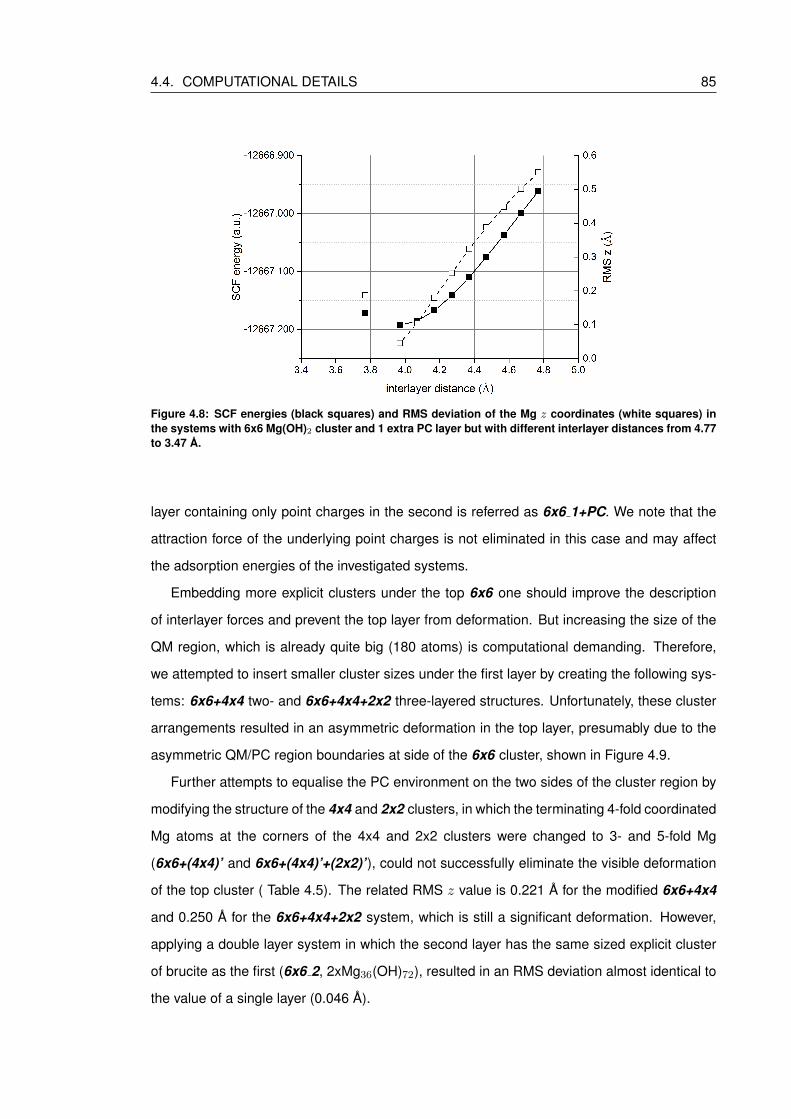
4.4. COMPUTATIONAL DETAILS 85
Figure 4.8: SCF energies (black squares) and RMS deviation of the Mg z coordinates (white squares) inthe systems with 6x6 Mg(OH)2 cluster and 1 extra PC layer but with different interlayer distances from 4.77to 3.47 A.
layer containing only point charges in the second is referred as 6x6 1+PC. We note that the
attraction force of the underlying point charges is not eliminated in this case and may affect
the adsorption energies of the investigated systems.
Embedding more explicit clusters under the top 6x6 one should improve the description
of interlayer forces and prevent the top layer from deformation. But increasing the size of the
QM region, which is already quite big (180 atoms) is computational demanding. Therefore,
we attempted to insert smaller cluster sizes under the first layer by creating the following sys-
tems: 6x6+4x4 two- and 6x6+4x4+2x2 three-layered structures. Unfortunately, these cluster
arrangements resulted in an asymmetric deformation in the top layer, presumably due to the
asymmetric QM/PC region boundaries at side of the 6x6 cluster, shown in Figure 4.9.
Further attempts to equalise the PC environment on the two sides of the cluster region by
modifying the structure of the 4x4 and 2x2 clusters, in which the terminating 4-fold coordinated
Mg atoms at the corners of the 4x4 and 2x2 clusters were changed to 3- and 5-fold Mg
(6x6+(4x4)’ and 6x6+(4x4)’+(2x2)’), could not successfully eliminate the visible deformation
of the top cluster ( Table 4.5). The related RMS z value is 0.221 A for the modified 6x6+4x4
and 0.250 A for the 6x6+4x4+2x2 system, which is still a significant deformation. However,
applying a double layer system in which the second layer has the same sized explicit cluster
of brucite as the first (6x6 2, 2xMg36(OH)72), resulted in an RMS deviation almost identical to
the value of a single layer (0.046 A).

86CHAPTER 4. MODELLING THE (0001) BRUCITE SURFACE WITH THE PERIODIC
ELECTROSTATIC EMBEDDED CLUSTER METHOD
Figure 4.9: Side view of a system with two explicit Mg(OH)2 cluster (6x6+4x4) (a); and a system with threeexplicit clusters (6x6+4x4+2x2) (b). Because of the asymmetrical geometry of the smaller clusters, thedeformation in the left side of the upper cluster is greater. Atoms in the QM region are represented bywires, while the outer part by points. (Mg=green, O=red, H=grey)
Table 4.5: Comparison of SCF energies and RMS deviation of the Mg z coordinates in the first brucitelayer, for systems with more explicit layers within the cluster and with or without extra PC layers. (nxnrefers to the number of Mg atoms in the cluster, (nxn)’ refers to clusters with modified geometries)
total number of layers PC layers SCF energy (a.u) RMS z (A)
6x6+4x4
2 0 -18297.0529 0.2363 1 -18297.1564 0.2654 2 -18297.1564 0.2645 3 -18297.1564 0.265
6x6+4x4+2x2
3 0 -19705.0615 0.2674 1 -19705.0861 0.2705 2 -19705.0861 0.2706 3 -19705.0861 0.270
6x6+(4x4)’
2 0 -18297.2397 0.2213 1 -18297.3375 0.2484 2 -18297.3375 0.2465 3 -18297.3375 0.249
6x6+(4x4)’+(2x2)’
3 0 -19705.4253 0.250
6x6+6x6
2 0 -25333.7182 0.0463 1 -25333.9664 0.1274 2 -25333.9664 0.1295 3 -25333.9664 0.126
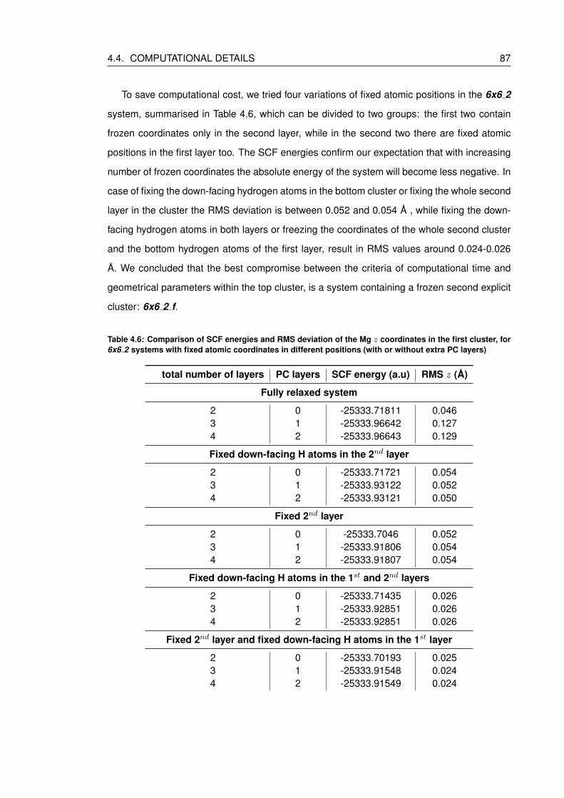
4.4. COMPUTATIONAL DETAILS 87
To save computational cost, we tried four variations of fixed atomic positions in the 6x6 2
system, summarised in Table 4.6, which can be divided to two groups: the first two contain
frozen coordinates only in the second layer, while in the second two there are fixed atomic
positions in the first layer too. The SCF energies confirm our expectation that with increasing
number of frozen coordinates the absolute energy of the system will become less negative. In
case of fixing the down-facing hydrogen atoms in the bottom cluster or fixing the whole second
layer in the cluster the RMS deviation is between 0.052 and 0.054 A , while fixing the down-
facing hydrogen atoms in both layers or freezing the coordinates of the whole second cluster
and the bottom hydrogen atoms of the first layer, result in RMS values around 0.024-0.026
A. We concluded that the best compromise between the criteria of computational time and
geometrical parameters within the top cluster, is a system containing a frozen second explicit
cluster: 6x6 2 f.
Table 4.6: Comparison of SCF energies and RMS deviation of the Mg z coordinates in the first cluster, for6x6 2 systems with fixed atomic coordinates in different positions (with or without extra PC layers)
total number of layers PC layers SCF energy (a.u) RMS z (A)
Fully relaxed system
2 0 -25333.71811 0.0463 1 -25333.96642 0.1274 2 -25333.96643 0.129
Fixed down-facing H atoms in the 2nd layer
2 0 -25333.71721 0.0543 1 -25333.93122 0.0524 2 -25333.93121 0.050
Fixed 2nd layer
2 0 -25333.7046 0.0523 1 -25333.91806 0.0544 2 -25333.91807 0.054
Fixed down-facing H atoms in the 1st and 2nd layers
2 0 -25333.71435 0.0263 1 -25333.92851 0.0264 2 -25333.92851 0.026
Fixed 2nd layer and fixed down-facing H atoms in the 1st layer
2 0 -25333.70193 0.0253 1 -25333.91548 0.0244 2 -25333.91549 0.024
88CHAPTER 4. MODELLING THE (0001) BRUCITE SURFACE WITH THE PERIODIC
ELECTROSTATIC EMBEDDED CLUSTER METHOD
4.4.2 Periodic DFT models
We chose the CRYSTAL14 code[138, 141] to model the brucite (0001) surface with periodic
DFT, since this program allows us to use atom-centred basis sets, as used in TURBOMOLE.
The TPSS meta-GGA exchange correlation functional, which was used for the development
of the PEECM model, is not available in this code. Since TPSS was developed by Perdew
and coworkers based on the same philosophy as PBE exchange-correlation functional[74],
we decided to use the latter in CRYSTAL14. PBE is one of the most commonly used GGA
functionals in solid state chemistry, besides, the general gradient approximation level of theory
gave good agreement with the experimental parameters of brucite in previous studies.[201,
202, 209, 210] Following on from the work of Ungliengo et al.[206], we compared the geo-
metrical parameters obtained with the use of PBE to the Grimme type dispersion corrected
PBE-D functional[83, 84]. Since PBE-D resulted in an interlayer distance 0.15 A less than the
experimental values, we decided to continue with PBE, see Table 4.7.
Polarised triple-ζ basis sets, derived specifically for solid state calculations by Peintinger
et al.[247] were used for the surface atoms (Mg pob TZVP 2012, O pob TZVP 2012, and
H pob TZVP 2012) along with the Ca atom in the substitution study presented in section
4.5.3 (Ca pob TZVP 2102). In the case of Sr, the Sr HAYWSC-311(d11f)G basis set[248]
was used for geometry optimisations, whilst single point energies were calculated using dou-
bly polarised triple-ζ basis sets for the valence electrons with the ECP28MWB multi-electron
fit quasi-pseudopotential on the electrons of the core 1s-3d orbitals.[97] We used the 0D
MOLECULE option of CRYSTAL14 for the single point energies of the isolated ions in sec-
tion 4.5.1 and for the solvated Sr(OH)2 complex in section 4.5.4, which allows to optimise
systems as non-periodic, isolated structures in vacuum.iii
For the model studies presented in sections 4.5.3 and 4.5.4, to make comparison between
the two different methods possible, we used the PBE functional with the same computational
parameters for the PEECM calculations as was detailed for periodic DFT. Although for the em-
bedded cluster structures def2-SVP basis sets were used for the geometry optimisation, single
point energies were obtained after geometry optimisation with the above defined CRYSTAL14
basis functions.
iiiSince we were using the same computational parameters, the calculated energies with both CRYSTAL14 andTURBOMOLE were essentially the same for isolated ions in vacuum (less than 10−6 a.u. difference).
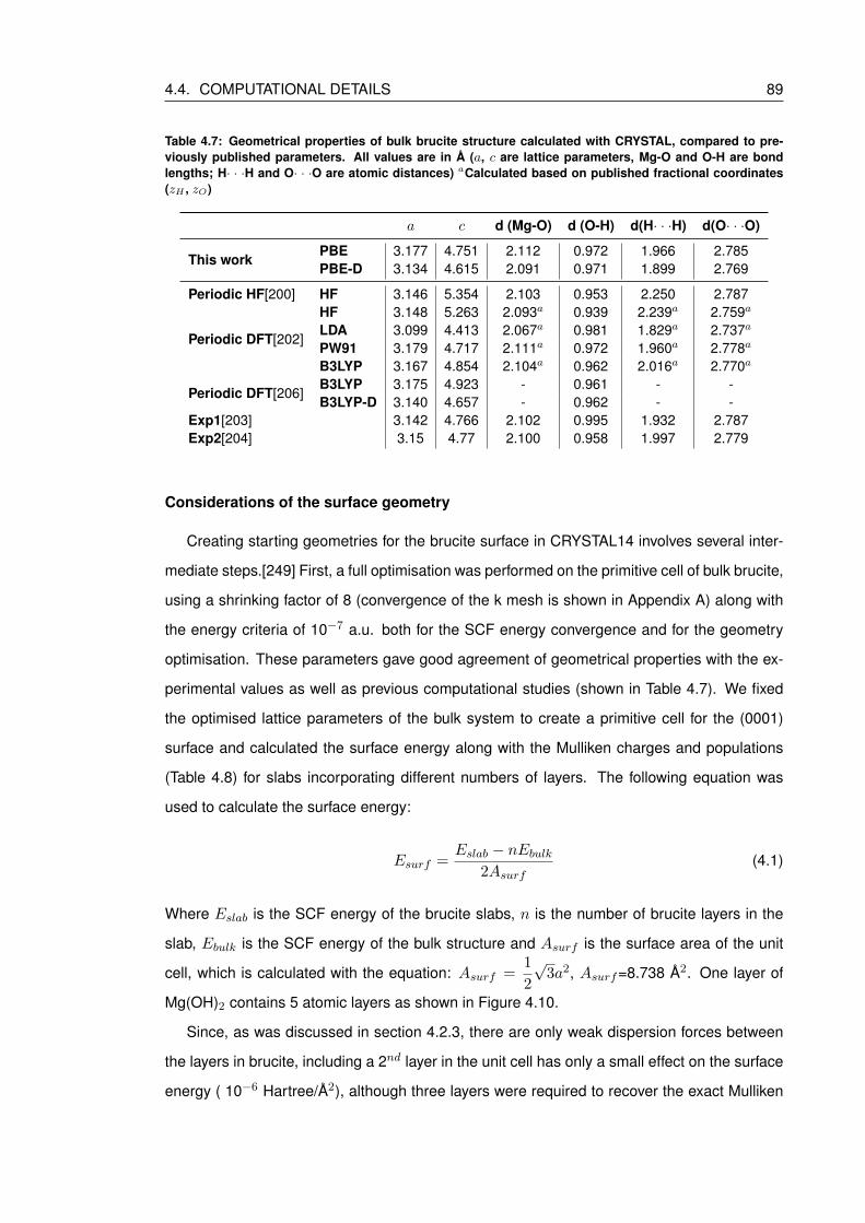
4.4. COMPUTATIONAL DETAILS 89
Table 4.7: Geometrical properties of bulk brucite structure calculated with CRYSTAL, compared to pre-viously published parameters. All values are in A (a, c are lattice parameters, Mg-O and O-H are bondlengths; H· · ·H and O· · ·O are atomic distances) aCalculated based on published fractional coordinates(zH , zO)
a c d (Mg-O) d (O-H) d(H· · ·H) d(O· · ·O)
This workPBE 3.177 4.751 2.112 0.972 1.966 2.785PBE-D 3.134 4.615 2.091 0.971 1.899 2.769
Periodic HF[200] HF 3.146 5.354 2.103 0.953 2.250 2.787
Periodic DFT[202]
HF 3.148 5.263 2.093a 0.939 2.239a 2.759a
LDA 3.099 4.413 2.067a 0.981 1.829a 2.737a
PW91 3.179 4.717 2.111a 0.972 1.960a 2.778a
B3LYP 3.167 4.854 2.104a 0.962 2.016a 2.770a
Periodic DFT[206]B3LYP 3.175 4.923 - 0.961 - -B3LYP-D 3.140 4.657 - 0.962 - -
Exp1[203] 3.142 4.766 2.102 0.995 1.932 2.787Exp2[204] 3.15 4.77 2.100 0.958 1.997 2.779
Considerations of the surface geometry
Creating starting geometries for the brucite surface in CRYSTAL14 involves several inter-
mediate steps.[249] First, a full optimisation was performed on the primitive cell of bulk brucite,
using a shrinking factor of 8 (convergence of the k mesh is shown in Appendix A) along with
the energy criteria of 10−7 a.u. both for the SCF energy convergence and for the geometry
optimisation. These parameters gave good agreement of geometrical properties with the ex-
perimental values as well as previous computational studies (shown in Table 4.7). We fixed
the optimised lattice parameters of the bulk system to create a primitive cell for the (0001)
surface and calculated the surface energy along with the Mulliken charges and populations
(Table 4.8) for slabs incorporating different numbers of layers. The following equation was
used to calculate the surface energy:
Esurf =Eslab − nEbulk
2Asurf(4.1)
Where Eslab is the SCF energy of the brucite slabs, n is the number of brucite layers in the
slab, Ebulk is the SCF energy of the bulk structure and Asurf is the surface area of the unit
cell, which is calculated with the equation: Asurf =1
2
√3a2, Asurf=8.738 A2. One layer of
Mg(OH)2 contains 5 atomic layers as shown in Figure 4.10.
Since, as was discussed in section 4.2.3, there are only weak dispersion forces between
the layers in brucite, including a 2nd layer in the unit cell has only a small effect on the surface
energy ( 10−6 Hartree/A2), although three layers were required to recover the exact Mulliken
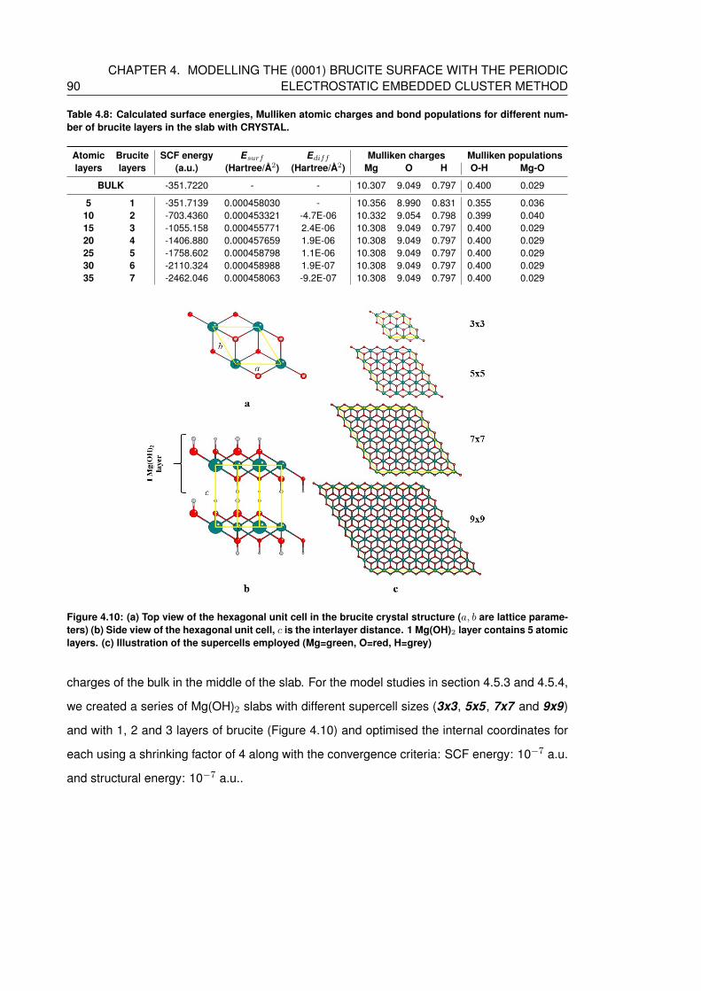
90CHAPTER 4. MODELLING THE (0001) BRUCITE SURFACE WITH THE PERIODIC
ELECTROSTATIC EMBEDDED CLUSTER METHOD
Table 4.8: Calculated surface energies, Mulliken atomic charges and bond populations for different num-ber of brucite layers in the slab with CRYSTAL.
Atomiclayers
Brucitelayers
SCF energy(a.u.)
Esurf
(Hartree/A2)Ediff
(Hartree/A2)Mulliken charges Mulliken populations
Mg O H O-H Mg-O
BULK -351.7220 - - 10.307 9.049 0.797 0.400 0.029
5 1 -351.7139 0.000458030 - 10.356 8.990 0.831 0.355 0.03610 2 -703.4360 0.000453321 -4.7E-06 10.332 9.054 0.798 0.399 0.04015 3 -1055.158 0.000455771 2.4E-06 10.308 9.049 0.797 0.400 0.02920 4 -1406.880 0.000457659 1.9E-06 10.308 9.049 0.797 0.400 0.02925 5 -1758.602 0.000458798 1.1E-06 10.308 9.049 0.797 0.400 0.02930 6 -2110.324 0.000458988 1.9E-07 10.308 9.049 0.797 0.400 0.02935 7 -2462.046 0.000458063 -9.2E-07 10.308 9.049 0.797 0.400 0.029
Figure 4.10: (a) Top view of the hexagonal unit cell in the brucite crystal structure (a, b are lattice parame-ters) (b) Side view of the hexagonal unit cell, c is the interlayer distance. 1 Mg(OH)2 layer contains 5 atomiclayers. (c) Illustration of the supercells employed (Mg=green, O=red, H=grey)
charges of the bulk in the middle of the slab. For the model studies in section 4.5.3 and 4.5.4,
we created a series of Mg(OH)2 slabs with different supercell sizes (3x3, 5x5, 7x7 and 9x9)
and with 1, 2 and 3 layers of brucite (Figure 4.10) and optimised the internal coordinates for
each using a shrinking factor of 4 along with the convergence criteria: SCF energy: 10−7 a.u.
and structural energy: 10−7 a.u..
4.5. RESULTS 91
4.5 ResultsThe primary goal of the model studies presented in this section is to test the reliability
of the embedded cluster model developed for the brucite (0001) surface. First, we examine
the adsorption of charged systems, by investigating the interaction of a series of s block ions
and a simple Sr2+ hydrate with brucite. Then, we move on to compare the embedded model
calculations with a more widely established method (periodic DFT); we perform a substitution
study for single ions into brucite and a second in which we look at the adsorption of differently
coordinated [Sr(OH)2(H2O)4] complexes on the surface, comparing their relative stability. We
also used the periodic DFT model to carry out cell size studies on the systems of interest
and to (indirectly) verify the size of the quantum chemically treated cluster in the PEECM
approach.
Note that the adsorption and substitution energies presented in sections 4.5.1 and 4.5.3
are calculated without considering the effects of solvation on the adsorbed or substituted ions,
and the model systems of 4.5.2 and 4.5.4 only contain a few explicit solvent molecules. This
has been done partly to avoid the extra variability and complication that will inevitably arise
from the treatment of solvation and because the purpose of these calculations is to provide as
direct and straightforward a comparison of periodic DFT and PEECM as possible.
4.5.1 Single ion adsorption of Sr2+ and other s block elements on brucite
We calculated adsorption energies for a series of ions: Na+, Rb+, Cs+ and Mg2+, Sr2+,
Ba2+ from which Na+, Cs+, Sr2+ and Mg2+ are known to exist in the aqueous phase in Mag-
nox storage ponds.[2] As described in the Introduction 1.2, we have a special interest in 90Sr2+
and 137Cs+, as their adsorption behaviour is especially important in the waste treatment pro-
cess. We included Rb+ and Ba2+ to make the series of the singly and double charged ions
complete, and to allow us to test if the adsorption energies follow the trend expected based
on the ionic radii and charges, i.e. the dications should have a stronger interaction with the
surface, and the interaction energy should decrease with decreasing ionic charge density.
The following equation was used to calculate the adsorption energies presented in Table
4.11:
Eads = Ecomplex − (Ebrucite + EM2+) (4.2)
Ecomplex is the SCF energy of the adsorbed ion with the surface, while Ebrucite is the energy
of the brucite surface model (6x6 1, 6x6 1+PC, or 6x6 2) and EM2+ is the energy of the
adsorbed ion.
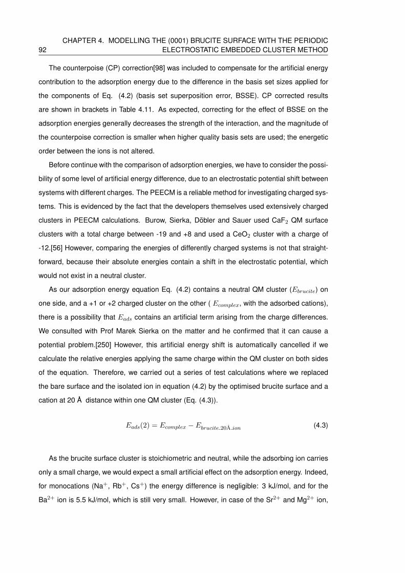
92CHAPTER 4. MODELLING THE (0001) BRUCITE SURFACE WITH THE PERIODIC
ELECTROSTATIC EMBEDDED CLUSTER METHOD
The counterpoise (CP) correction[98] was included to compensate for the artificial energy
contribution to the adsorption energy due to the difference in the basis set sizes applied for
the components of Eq. (4.2) (basis set superposition error, BSSE). CP corrected results
are shown in brackets in Table 4.11. As expected, correcting for the effect of BSSE on the
adsorption energies generally decreases the strength of the interaction, and the magnitude of
the counterpoise correction is smaller when higher quality basis sets are used; the energetic
order between the ions is not altered.
Before continue with the comparison of adsorption energies, we have to consider the possi-
bility of some level of artificial energy difference, due to an electrostatic potential shift between
systems with different charges. The PEECM is a reliable method for investigating charged sys-
tems. This is evidenced by the fact that the developers themselves used extensively charged
clusters in PEECM calculations. Burow, Sierka, Dobler and Sauer used CaF2 QM surface
clusters with a total charge between -19 and +8 and used a CeO2 cluster with a charge of
-12.[56] However, comparing the energies of differently charged systems is not that straight-
forward, because their absolute energies contain a shift in the electrostatic potential, which
would not exist in a neutral cluster.
As our adsorption energy equation Eq. (4.2) contains a neutral QM cluster (Ebrucite) on
one side, and a +1 or +2 charged cluster on the other ( Ecomplex, with the adsorbed cations),
there is a possibility that Eads contains an artificial term arising from the charge differences.
We consulted with Prof Marek Sierka on the matter and he confirmed that it can cause a
potential problem.[250] However, this artificial energy shift is automatically cancelled if we
calculate the relative energies applying the same charge within the QM cluster on both sides
of the equation. Therefore, we carried out a series of test calculations where we replaced
the bare surface and the isolated ion in equation (4.2) by the optimised brucite surface and a
cation at 20 A distance within one QM cluster (Eq. (4.3)).
Eads(2) = Ecomplex − Ebrucite 20A ion (4.3)
As the brucite surface cluster is stoichiometric and neutral, while the adsorbing ion carries
only a small charge, we would expect a small artificial effect on the adsorption energy. Indeed,
for monocations (Na+, Rb+, Cs+) the energy difference is negligible: 3 kJ/mol, and for the
Ba2+ ion is 5.5 kJ/mol, which is still very small. However, in case of the Sr2+ and Mg2+ ion,
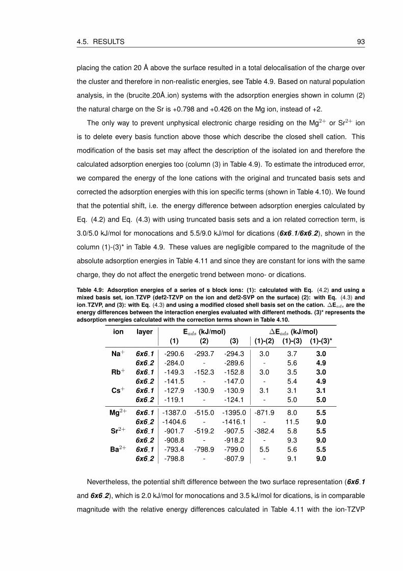
4.5. RESULTS 93
placing the cation 20 A above the surface resulted in a total delocalisation of the charge over
the cluster and therefore in non-realistic energies, see Table 4.9. Based on natural population
analysis, in the (brucite 20A ion) systems with the adsorption energies shown in column (2)
the natural charge on the Sr is +0.798 and +0.426 on the Mg ion, instead of +2.
The only way to prevent unphysical electronic charge residing on the Mg2+ or Sr2+ ion
is to delete every basis function above those which describe the closed shell cation. This
modification of the basis set may affect the description of the isolated ion and therefore the
calculated adsorption energies too (column (3) in Table 4.9). To estimate the introduced error,
we compared the energy of the lone cations with the original and truncated basis sets and
corrected the adsorption energies with this ion specific terms (shown in Table 4.10). We found
that the potential shift, i.e. the energy difference between adsorption energies calculated by
Eq. (4.2) and Eq. (4.3) with using truncated basis sets and a ion related correction term, is
3.0/5.0 kJ/mol for monocations and 5.5/9.0 kJ/mol for dications (6x6 1/6x6 2), shown in the
column (1)-(3)* in Table 4.9. These values are negligible compared to the magnitude of the
absolute adsorption energies in Table 4.11 and since they are constant for ions with the same
charge, they do not affect the energetic trend between mono- or dications.
Table 4.9: Adsorption energies of a series of s block ions: (1): calculated with Eq. (4.2) and using amixed basis set, ion TZVP (def2-TZVP on the ion and def2-SVP on the surface) (2): with Eq. (4.3) andion TZVP, and (3): with Eq. (4.3) and using a modified closed shell basis set on the cation. ∆Eads are theenergy differences between the interaction energies evaluated with different methods. (3)* represents theadsorption energies calculated with the correction terms shown in Table 4.10.
ion layer Eads (kJ/mol) ∆Eads (kJ/mol)(1) (2) (3) (1)-(2) (1)-(3) (1)-(3)*
Na+ 6x6 1 -290.6 -293.7 -294.3 3.0 3.7 3.06x6 2 -284.0 - -289.6 - 5.6 4.9
Rb+ 6x6 1 -149.3 -152.3 -152.8 3.0 3.5 3.06x6 2 -141.5 - -147.0 - 5.4 4.9
Cs+ 6x6 1 -127.9 -130.9 -130.9 3.1 3.1 3.16x6 2 -119.1 - -124.1 - 5.0 5.0
Mg2+ 6x6 1 -1387.0 -515.0 -1395.0 -871.9 8.0 5.56x6 2 -1404.6 - -1416.1 - 11.5 9.0
Sr2+ 6x6 1 -901.7 -519.2 -907.5 -382.4 5.8 5.56x6 2 -908.8 - -918.2 - 9.3 9.0
Ba2+ 6x6 1 -793.4 -798.9 -799.0 5.5 5.6 5.56x6 2 -798.8 - -807.9 - 9.1 9.0
Nevertheless, the potential shift difference between the two surface representation (6x6 1
and 6x6 2), which is 2.0 kJ/mol for monocations and 3.5 kJ/mol for dications, is in comparable
magnitude with the relative energy differences calculated in Table 4.11 with the ion-TZVP
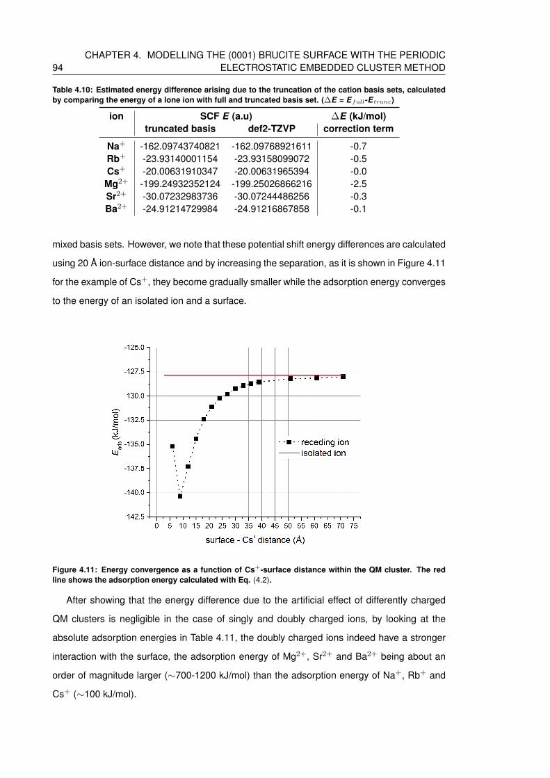
94CHAPTER 4. MODELLING THE (0001) BRUCITE SURFACE WITH THE PERIODIC
ELECTROSTATIC EMBEDDED CLUSTER METHOD
Table 4.10: Estimated energy difference arising due to the truncation of the cation basis sets, calculatedby comparing the energy of a lone ion with full and truncated basis set. (∆E = Efull-Etrunc)
ion SCF E (a.u) ∆E (kJ/mol)truncated basis def2-TZVP correction term
Na+ -162.09743740821 -162.09768921611 -0.7Rb+ -23.93140001154 -23.93158099072 -0.5Cs+ -20.00631910347 -20.00631965394 -0.0
Mg2+ -199.24932352124 -199.25026866216 -2.5Sr2+ -30.07232983736 -30.07244486256 -0.3Ba2+ -24.91214729984 -24.91216867858 -0.1
mixed basis sets. However, we note that these potential shift energy differences are calculated
using 20 A ion-surface distance and by increasing the separation, as it is shown in Figure 4.11
for the example of Cs+, they become gradually smaller while the adsorption energy converges
to the energy of an isolated ion and a surface.
Figure 4.11: Energy convergence as a function of Cs+-surface distance within the QM cluster. The redline shows the adsorption energy calculated with Eq. (4.2).
After showing that the energy difference due to the artificial effect of differently charged
QM clusters is negligible in the case of singly and doubly charged ions, by looking at the
absolute adsorption energies in Table 4.11, the doubly charged ions indeed have a stronger
interaction with the surface, the adsorption energy of Mg2+, Sr2+ and Ba2+ being about an
order of magnitude larger (∼700-1200 kJ/mol) than the adsorption energy of Na+, Rb+ and
Cs+ (∼100 kJ/mol).
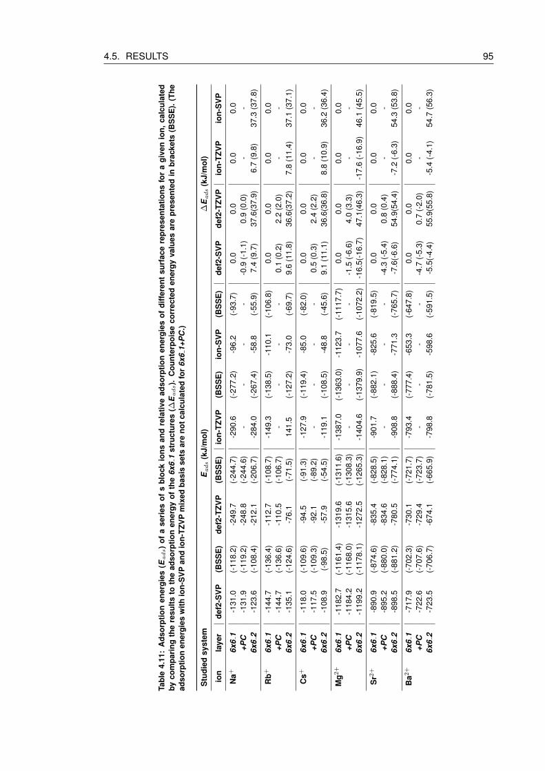
4.5. RESULTS 95
Tabl
e4.
11:
Ads
orpt
ion
ener
gies
(Eads)
ofa
seri
esof
sbl
ock
ions
and
rela
tive
adso
rptio
nen
ergi
esof
diff
eren
tsu
rfac
ere
pres
enta
tions
for
agi
ven
ion,
calc
ulat
edby
com
pari
ngth
ere
sults
toth
ead
sorp
tion
ener
gyof
the
6x6
1st
ruct
ures
(∆E
ads).
Cou
nter
pois
eco
rrec
ted
ener
gyva
lues
are
pres
ente
din
brac
kets
(BS
SE
).(T
head
sorp
tion
ener
gies
with
ion-
SV
Pan
dio
n-TZ
VP
mix
edba
sis
sets
are
notc
alcu
late
dfo
r6x
61+
PC
.)
Stu
died
syst
emEads
(kJ/
mol
)∆
Eads
(kJ/
mol
)
ion
laye
rde
f2-S
VP
(BS
SE
)de
f2-T
ZVP
(BS
SE
)io
n-TZ
VP
(BS
SE
)io
n-S
VP
(BS
SE
)de
f2-S
VP
def2
-TZV
Pio
n-TZ
VP
ion-
SV
P
Na+
6x6
1-1
31.0
(-11
8.2)
-249
.7(-
244.
7)-2
90.6
(-27
7.2)
-96.
2(-
93.7
)0.
00.
00.
00.
0+P
C-1
31.9
(-11
9.2)
-248
.8(-
244.
6)-
--
--0
.9(-
1.1)
0.9
(0.0
)-
-6x
62
-123
.6(-
108.
4)-2
12.1
(-20
6.7)
-284
.0(-
267.
4)-5
8.8
(-55
.9)
7.4
(9.7
)37
.6(3
7.9)
6.7
(9.8
)37
.3(3
7.8)
Rb+
6x6
1-1
44.7
(-13
6.4)
-112
.7(-
108.
7)-1
49.3
(-13
8.5)
-110
.1(-
106.
8)0.
00.
00.
00.
0+P
C-1
44.7
(-13
6.6)
-110
.5(-
106.
7)-
--
-0.
1(0
.2)
2.2
(2.0
)-
-6x
62
-135
.1(-
124.
6)-7
6.1
(-71
.5)
141.
5(-
127.
2)-7
3.0
(-69
.7)
9.6
(11.
8)36
.6(3
7.2)
7.8
(11.
4)37
.1(3
7.1)
Cs+
6x6
1-1
18.0
(-10
9.6)
-94.
5(-
91.3
)-1
27.9
(-11
9.4)
-85.
0(-
82.0
)0.
00.
00.
00.
0+P
C-1
17.5
(-10
9.3)
-92.
1(-
89.2
)-
--
-0.
5(0
.3)
2.4
(2.2
)-
-6x
62
-108
.9(-
98.5
)-5
7.9
(-54
.5)
-119
.1(-
108.
5)-4
8.8
(-45
.6)
9.1
(11.
1)36
.6(3
6.8)
8.8
(10.
9)36
.2(3
6.4)
Mg2
+6x
61
-118
2.7
(-11
61.4
)-1
319.
6(-
1311
.6)
-138
7.0
(-13
63.0
)-1
123.
7(-
1117
.7)
0.0
0.0
0.0
0.0
+PC
-118
4.2
(-11
68.0
)-1
315.
6(-
1308
.3)
--
--
-1.5
(-6.
6)4.
0(3
.3)
--
6x6
2-1
199.
2(-
1178
.1)
-127
2.5
(-12
65.3
)-1
404.
6(-
1379
.9)
-107
7.6
(-10
72.2
)-1
6.5(
-16.
7)47
.1(4
6.3)
-17.
6(-
16.9
)46
.1(4
5.5)
Sr2
+6x
61
-890
.9(-
874.
6)-8
35.4
(-82
8.5)
-901
.7(-
882.
1)-8
25.6
(-81
9.5)
0.0
0.0
0.0
0.0
+PC
-895
.2(-
880.
0)-8
34.6
(-82
8.1)
--
--
-4.3
(-5.
4)0.
8(0
.4)
--
6x6
2-8
98.5
(-88
1.2)
-780
.5(-
774.
1)-9
08.8
(-88
8.4)
-771
.3(-
765.
7)-7
.6(-
6.6)
54.9
(54.
4)-7
.2(-
6.3)
54.3
(53.
8)
Ba2
+6x
61
-717
.9(-
702.
3)-7
30.1
(-72
1.7)
-793
.4(-
777.
4)-6
53.3
(-64
7.8)
0.0
0.0
0.0
0.0
+PC
-722
.6(-
707.
6)-7
29.4
(-72
3.7)
--
--
-4.7
(-5.
3)0.
7(-
2.0)
--
6x6
2-7
23.5
(-70
6.7)
-674
.1(-
665.
9)-7
98.8
(-78
1.5)
-598
.6(-
591.
5)-5
.5(-
4.4)
55.9
(55.
8)-5
.4(-
4.1)
54.7
(56.
3)
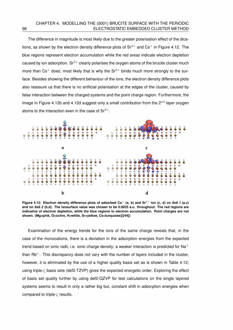
96CHAPTER 4. MODELLING THE (0001) BRUCITE SURFACE WITH THE PERIODIC
ELECTROSTATIC EMBEDDED CLUSTER METHOD
The difference in magnitude is most likely due to the greater polarisation effect of the dica-
tions, as shown by the electron density difference plots of Sr2+ and Cs+ in Figure 4.12. The
blue regions represent electron accumulation while the red areas indicate electron depletion
caused by ion adsorption. Sr2+ clearly polarises the oxygen atoms of the brucite cluster much
more than Cs+ does; most likely that is why the Sr2+ binds much more strongly to the sur-
face. Besides showing the different behaviour of the ions, the electron density difference plots
also reassure us that there is no artificial polarisation at the edges of the cluster, caused by
false interaction between the charged systems and the point charge region. Furthermore, the
image in Figure 4.12b and 4.12d suggest only a small contribution from the 2nd layer oxygen
atoms to the interaction even in the case of Sr2+.
Figure 4.12: Electron density difference plots of adsorbed Cs+ (a, b) and Sr2+ ion (c, d) on 6x6 1 (a,c)and on 6x6 2 (b,d). The isosurface value was chosen to be 0.0025 a.u. throughout. The red regions areindicative of electron depletion, while the blue regions to electron accumulation. Point charges are notshown. (Mg=pink, O=ochre, H=white, Sr=yellow, Cs=turquoise)[244])
Examination of the energy trends for the ions of the same charge reveals that, in the
case of the monocations, there is a deviation in the adsorption energies from the expected
trend based on ionic radii, i.e. ionic charge density; a weaker interaction is predicted for Na+
than Rb+. This discrepancy does not vary with the number of layers included in the cluster,
however, it is eliminated by the use of a higher quality basis set as is shown in Table 4.12;
using triple-ζ basis sets (def2-TZVP) gives the expected energetic order. Exploring the effect
of basis set quality further by using def2-QZVP for test calculations on the single layered
systems seems to result in only a rather big but, constant shift in adsorption energies when
compared to triple-ζ results.
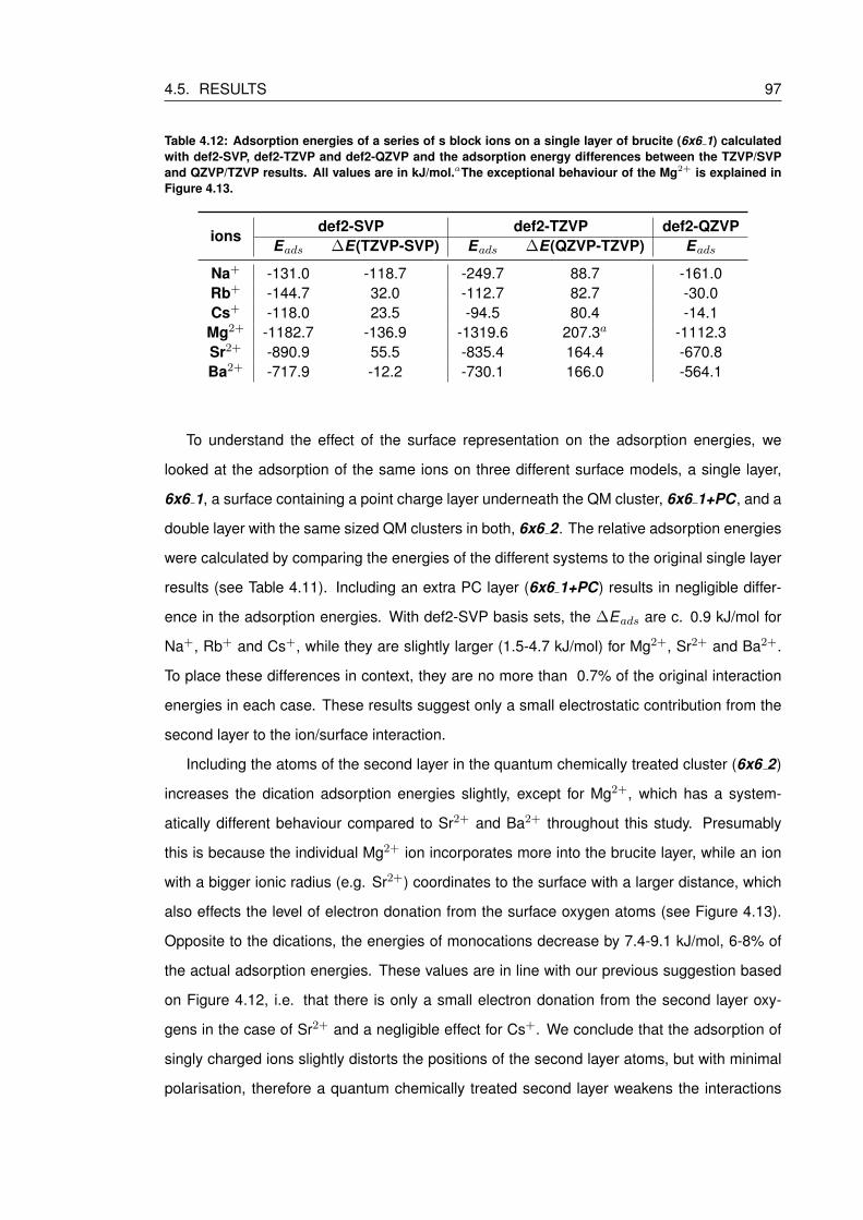
4.5. RESULTS 97
Table 4.12: Adsorption energies of a series of s block ions on a single layer of brucite (6x6 1) calculatedwith def2-SVP, def2-TZVP and def2-QZVP and the adsorption energy differences between the TZVP/SVPand QZVP/TZVP results. All values are in kJ/mol.aThe exceptional behaviour of the Mg2+ is explained inFigure 4.13.
ionsdef2-SVP def2-TZVP def2-QZVP
Eads ∆E(TZVP-SVP) Eads ∆E(QZVP-TZVP) Eads
Na+ -131.0 -118.7 -249.7 88.7 -161.0Rb+ -144.7 32.0 -112.7 82.7 -30.0Cs+ -118.0 23.5 -94.5 80.4 -14.1
Mg2+ -1182.7 -136.9 -1319.6 207.3a -1112.3Sr2+ -890.9 55.5 -835.4 164.4 -670.8Ba2+ -717.9 -12.2 -730.1 166.0 -564.1
To understand the effect of the surface representation on the adsorption energies, we
looked at the adsorption of the same ions on three different surface models, a single layer,
6x6 1, a surface containing a point charge layer underneath the QM cluster, 6x6 1+PC, and a
double layer with the same sized QM clusters in both, 6x6 2. The relative adsorption energies
were calculated by comparing the energies of the different systems to the original single layer
results (see Table 4.11). Including an extra PC layer (6x6 1+PC) results in negligible differ-
ence in the adsorption energies. With def2-SVP basis sets, the ∆Eads are c. 0.9 kJ/mol for
Na+, Rb+ and Cs+, while they are slightly larger (1.5-4.7 kJ/mol) for Mg2+, Sr2+ and Ba2+.
To place these differences in context, they are no more than 0.7% of the original interaction
energies in each case. These results suggest only a small electrostatic contribution from the
second layer to the ion/surface interaction.
Including the atoms of the second layer in the quantum chemically treated cluster (6x6 2)
increases the dication adsorption energies slightly, except for Mg2+, which has a system-
atically different behaviour compared to Sr2+ and Ba2+ throughout this study. Presumably
this is because the individual Mg2+ ion incorporates more into the brucite layer, while an ion
with a bigger ionic radius (e.g. Sr2+) coordinates to the surface with a larger distance, which
also effects the level of electron donation from the surface oxygen atoms (see Figure 4.13).
Opposite to the dications, the energies of monocations decrease by 7.4-9.1 kJ/mol, 6-8% of
the actual adsorption energies. These values are in line with our previous suggestion based
on Figure 4.12, i.e. that there is only a small electron donation from the second layer oxy-
gens in the case of Sr2+ and a negligible effect for Cs+. We conclude that the adsorption of
singly charged ions slightly distorts the positions of the second layer atoms, but with minimal
polarisation, therefore a quantum chemically treated second layer weakens the interactions
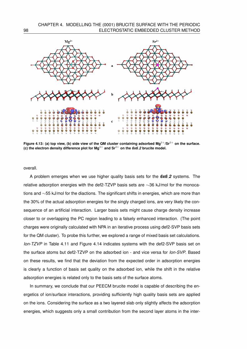
98CHAPTER 4. MODELLING THE (0001) BRUCITE SURFACE WITH THE PERIODIC
ELECTROSTATIC EMBEDDED CLUSTER METHOD
Figure 4.13: (a) top view, (b) side view of the QM cluster containing adsorbed Mg2+/Sr2+ on the surface.(c) the electron density difference plot for Mg2+ and Sr2+ on the 6x6 2 brucite model.
overall.
A problem emerges when we use higher quality basis sets for the 6x6 2 systems. The
relative adsorption energies with the def2-TZVP basis sets are ∼36 kJ/mol for the monoca-
tions and ∼55 kJ/mol for the diactions. The significant shifts in energies, which are more than
the 30% of the actual adsorption energies for the singly charged ions, are very likely the con-
sequence of an artificial interaction. Larger basis sets might cause charge density increase
closer to or overlapping the PC region leading to a falsely enhanced interaction. (The point
charges were originally calculated with NPA in an iterative process using def2-SVP basis sets
for the QM cluster). To probe this further, we explored a range of mixed basis set calculations.
Ion-TZVP in Table 4.11 and Figure 4.14 indicates systems with the def2-SVP basis set on
the surface atoms but def2-TZVP on the adsorbed ion - and vice versa for Ion-SVP. Based
on these results, we find that the deviation from the expected order in adsorption energies
is clearly a function of basis set quality on the adsorbed ion, while the shift in the relative
adsorption energies is related only to the basis sets of the surface atoms.
In summary, we conclude that our PEECM brucite model is capable of describing the en-
ergetics of ion/surface interactions, providing sufficiently high quality basis sets are applied
on the ions. Considering the surface as a two layered slab only slightly affects the adsorption
energies, which suggests only a small contribution from the second layer atoms in the inter-
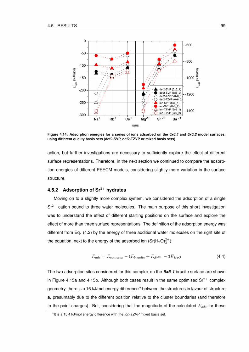
4.5. RESULTS 99
Figure 4.14: Adsorption energies for a series of ions adsorbed on the 6x6 1 and 6x6 2 model surfaces,using different quality basis sets (def2-SVP, def2-TZVP or mixed basis sets)
action, but further investigations are necessary to sufficiently explore the effect of different
surface representations. Therefore, in the next section we continued to compare the adsorp-
tion energies of different PEECM models, considering slightly more variation in the surface
structure.
4.5.2 Adsorption of Sr2+ hydrates
Moving on to a slightly more complex system, we considered the adsorption of a single
Sr2+ cation bound to three water molecules. The main purpose of this short investigation
was to understand the effect of different starting positions on the surface and explore the
effect of more than three surface representations. The definition of the adsorption energy was
different from Eq. (4.2) by the energy of three additional water molecules on the right site of
the equation, next to the energy of the adsorbed ion (Sr(H2O)2+3 ):
Eads = Ecomplex − (Ebrucite + ESr2+ + 3EH2O (4.4)
The two adsorption sites considered for this complex on the 6x6 1 brucite surface are shown
in Figure 4.15a and 4.15b. Although both cases result in the same optimised Sr2+ complex
geometry, there is a 16 kJ/mol energy differenceiv between the structures in favour of structure
a, presumably due to the different position relative to the cluster boundaries (and therefore
to the point charges). But, considering that the magnitude of the calculated Eads for these
ivIt is a 15.4 kJ/mol energy difference with the ion-TZVP mixed basis set.
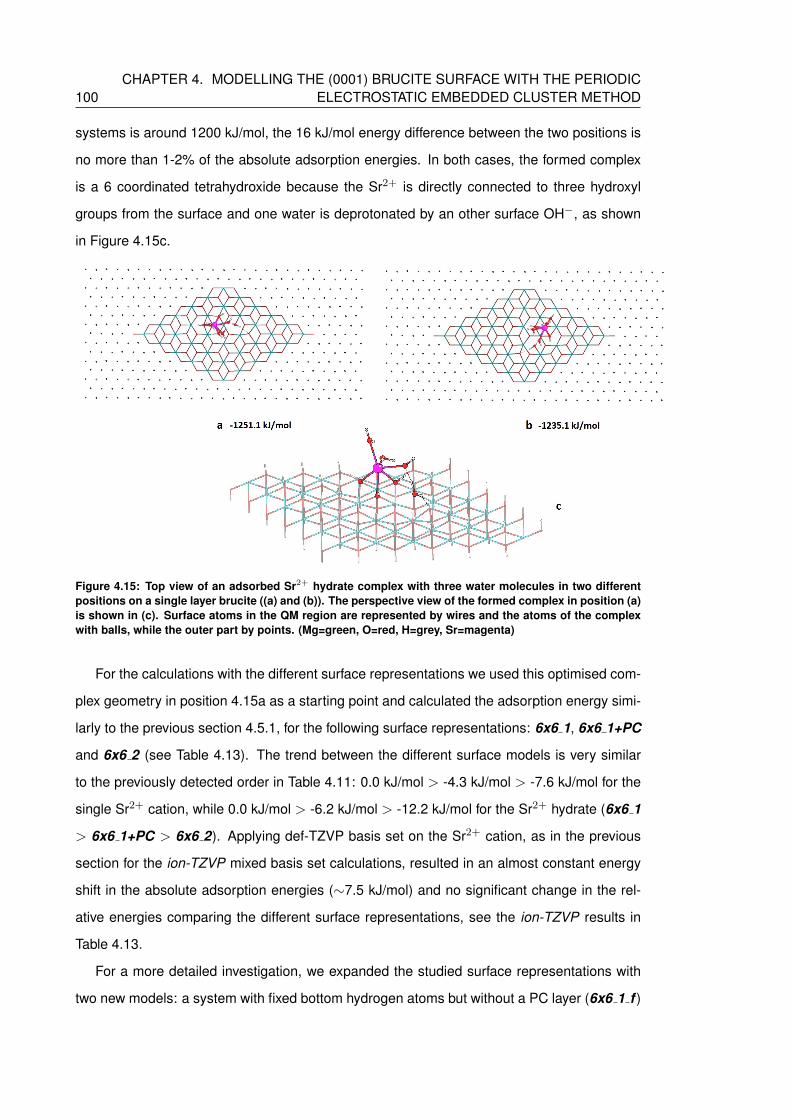
100CHAPTER 4. MODELLING THE (0001) BRUCITE SURFACE WITH THE PERIODIC
ELECTROSTATIC EMBEDDED CLUSTER METHOD
systems is around 1200 kJ/mol, the 16 kJ/mol energy difference between the two positions is
no more than 1-2% of the absolute adsorption energies. In both cases, the formed complex
is a 6 coordinated tetrahydroxide because the Sr2+ is directly connected to three hydroxyl
groups from the surface and one water is deprotonated by an other surface OH−, as shown
in Figure 4.15c.
Figure 4.15: Top view of an adsorbed Sr2+ hydrate complex with three water molecules in two differentpositions on a single layer brucite ((a) and (b)). The perspective view of the formed complex in position (a)is shown in (c). Surface atoms in the QM region are represented by wires and the atoms of the complexwith balls, while the outer part by points. (Mg=green, O=red, H=grey, Sr=magenta)
For the calculations with the different surface representations we used this optimised com-
plex geometry in position 4.15a as a starting point and calculated the adsorption energy simi-
larly to the previous section 4.5.1, for the following surface representations: 6x6 1, 6x6 1+PC
and 6x6 2 (see Table 4.13). The trend between the different surface models is very similar
to the previously detected order in Table 4.11: 0.0 kJ/mol > -4.3 kJ/mol > -7.6 kJ/mol for the
single Sr2+ cation, while 0.0 kJ/mol > -6.2 kJ/mol > -12.2 kJ/mol for the Sr2+ hydrate (6x6 1
> 6x6 1+PC > 6x6 2). Applying def-TZVP basis set on the Sr2+ cation, as in the previous
section for the ion-TZVP mixed basis set calculations, resulted in an almost constant energy
shift in the absolute adsorption energies (∼7.5 kJ/mol) and no significant change in the rel-
ative energies comparing the different surface representations, see the ion-TZVP results in
Table 4.13.
For a more detailed investigation, we expanded the studied surface representations with
two new models: a system with fixed bottom hydrogen atoms but without a PC layer (6x6 1 f )
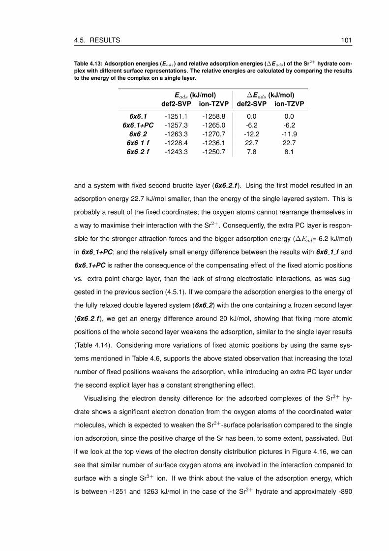
4.5. RESULTS 101
Table 4.13: Adsorption energies (Eads) and relative adsorption energies (∆Eads) of the Sr2+ hydrate com-plex with different surface representations. The relative energies are calculated by comparing the resultsto the energy of the complex on a single layer.
Eads (kJ/mol) ∆Eads (kJ/mol)def2-SVP ion-TZVP def2-SVP ion-TZVP
6x6 1 -1251.1 -1258.8 0.0 0.06x6 1+PC -1257.3 -1265.0 -6.2 -6.2
6x6 2 -1263.3 -1270.7 -12.2 -11.96x6 1 f -1228.4 -1236.1 22.7 22.76x6 2 f -1243.3 -1250.7 7.8 8.1
and a system with fixed second brucite layer (6x6 2 f ). Using the first model resulted in an
adsorption energy 22.7 kJ/mol smaller, than the energy of the single layered system. This is
probably a result of the fixed coordinates; the oxygen atoms cannot rearrange themselves in
a way to maximise their interaction with the Sr2+. Consequently, the extra PC layer is respon-
sible for the stronger attraction forces and the bigger adsorption energy (∆Ead=-6.2 kJ/mol)
in 6x6 1+PC; and the relatively small energy difference between the results with 6x6 1 f and
6x6 1+PC is rather the consequence of the compensating effect of the fixed atomic positions
vs. extra point charge layer, than the lack of strong electrostatic interactions, as was sug-
gested in the previous section (4.5.1). If we compare the adsorption energies to the energy of
the fully relaxed double layered system (6x6 2) with the one containing a frozen second layer
(6x6 2 f ), we get an energy difference around 20 kJ/mol, showing that fixing more atomic
positions of the whole second layer weakens the adsorption, similar to the single layer results
(Table 4.14). Considering more variations of fixed atomic positions by using the same sys-
tems mentioned in Table 4.6, supports the above stated observation that increasing the total
number of fixed positions weakens the adsorption, while introducing an extra PC layer under
the second explicit layer has a constant strengthening effect.
Visualising the electron density difference for the adsorbed complexes of the Sr2+ hy-
drate shows a significant electron donation from the oxygen atoms of the coordinated water
molecules, which is expected to weaken the Sr2+-surface polarisation compared to the single
ion adsorption, since the positive charge of the Sr has been, to some extent, passivated. But
if we look at the top views of the electron density distribution pictures in Figure 4.16, we can
see that similar number of surface oxygen atoms are involved in the interaction compared to
surface with a single Sr2+ ion. If we think about the value of the adsorption energy, which
is between -1251 and 1263 kJ/mol in the case of the Sr2+ hydrate and approximately -890
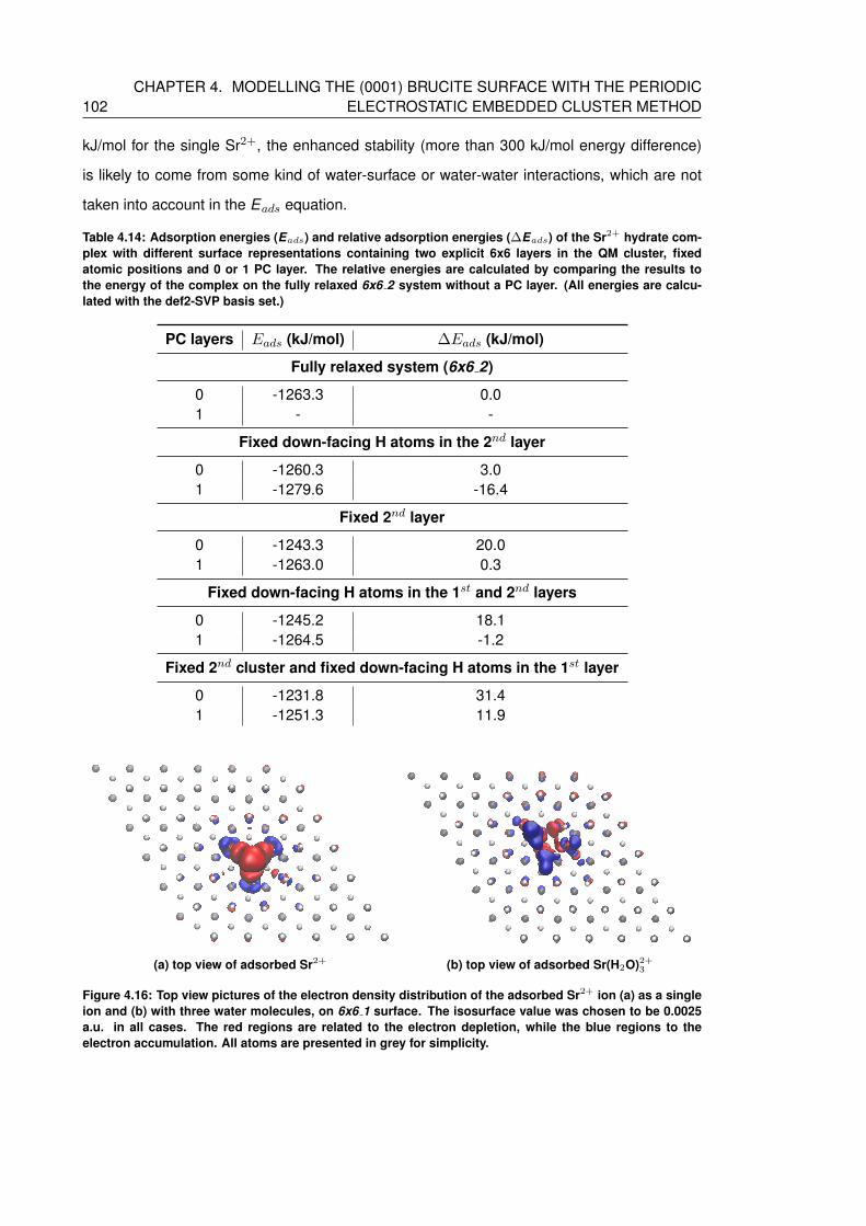
102CHAPTER 4. MODELLING THE (0001) BRUCITE SURFACE WITH THE PERIODIC
ELECTROSTATIC EMBEDDED CLUSTER METHOD
kJ/mol for the single Sr2+, the enhanced stability (more than 300 kJ/mol energy difference)
is likely to come from some kind of water-surface or water-water interactions, which are not
taken into account in the Eads equation.
Table 4.14: Adsorption energies (Eads) and relative adsorption energies (∆Eads) of the Sr2+ hydrate com-plex with different surface representations containing two explicit 6x6 layers in the QM cluster, fixedatomic positions and 0 or 1 PC layer. The relative energies are calculated by comparing the results tothe energy of the complex on the fully relaxed 6x6 2 system without a PC layer. (All energies are calcu-lated with the def2-SVP basis set.)
PC layers Eads (kJ/mol) ∆Eads (kJ/mol)
Fully relaxed system (6x6 2)
0 -1263.3 0.01 - -
Fixed down-facing H atoms in the 2nd layer
0 -1260.3 3.01 -1279.6 -16.4
Fixed 2nd layer
0 -1243.3 20.01 -1263.0 0.3
Fixed down-facing H atoms in the 1st and 2nd layers
0 -1245.2 18.11 -1264.5 -1.2
Fixed 2nd cluster and fixed down-facing H atoms in the 1st layer
0 -1231.8 31.41 -1251.3 11.9
(a) top view of adsorbed Sr2+ (b) top view of adsorbed Sr(H2O)2+3
Figure 4.16: Top view pictures of the electron density distribution of the adsorbed Sr2+ ion (a) as a singleion and (b) with three water molecules, on 6x6 1 surface. The isosurface value was chosen to be 0.0025a.u. in all cases. The red regions are related to the electron depletion, while the blue regions to theelectron accumulation. All atoms are presented in grey for simplicity.
4.5. RESULTS 103
Figure 4.17c with the surface model 6x6 2 reveals the top oxygen atoms in the second
layer are also involved in the electron donation, in agreement with the previous results in
Figure 4.12c, The fact that including an extra explicit layer strengthens the adsorption energy
by -12.2 kJ/mol, leads us to conclude that, while simply fixing the down-facing hydrogen atoms
and consider the second layer as PCs proved is not sufficient, modelling two explicit layer is
necessary for the description of the adsorption mechanism, even if the second layer is fixed.
Figure 4.17: Electron density distribution of the adsorbed Sr2+ ion with three water molecules, on a singlelayer brucite (a), on a cluster with fixed bottom hydrogen atoms and one PC layer (b) and on a surfacecontaining two explicit 6x6 clusters (c). The isosurface value was chosen to be 0.0025 in all cases. Thered regions are related to the electron depletion, while the blue regions to the electron accumulation. Thepoint charges are not represented on the pictures. (Mg=pink, O=ochre, H=white, Sr=yellow)
Based on the results presented in this section, we conclude that although the position
of the adsorbed complex compared to the cluster boundaries matters, the arising energy
difference is only a small portion of the absolute adsorption energy. Extending the studied
surface representations with 6x6 1 f and 6x6 2 f , showed that fixing atomic positions results
in smaller interaction energies. Further investigation of second layer effect confirmed that
minimum of one explicit layer is acceptable for the accurate description of the adsorption.
4.5.3 Substitution of Ca2+ and Sr2+ into brucite
Our next study was aimed to benchmark the PEECM results with periodic DFT methods
(CRYSTAL code). We used a substitution reaction of heavier group II ions for Mg2+ in brucite
(Ca2+, Sr2+). Besides comparing the reaction energies calculated with our PEECM model,
we study the effect of smaller/larger unit cells and the number of brucite layers on the ad-
sorption energy too. The substitution energies were calculated with both the PEECM model
and periodic DFT, using the same functional (PBE) and basis sets (section 4.4.2) with the two
different codes. We optimised structures with one (6x6 1) and two (6x6 2) layers included in
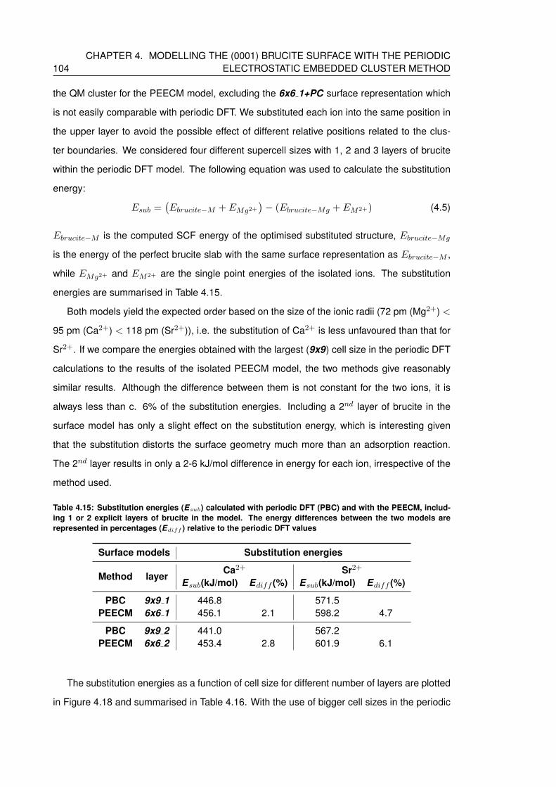
104CHAPTER 4. MODELLING THE (0001) BRUCITE SURFACE WITH THE PERIODIC
ELECTROSTATIC EMBEDDED CLUSTER METHOD
the QM cluster for the PEECM model, excluding the 6x6 1+PC surface representation which
is not easily comparable with periodic DFT. We substituted each ion into the same position in
the upper layer to avoid the possible effect of different relative positions related to the clus-
ter boundaries. We considered four different supercell sizes with 1, 2 and 3 layers of brucite
within the periodic DFT model. The following equation was used to calculate the substitution
energy:
Esub =(Ebrucite−M + EMg2+
)− (Ebrucite−Mg + EM2+) (4.5)
Ebrucite−M is the computed SCF energy of the optimised substituted structure, Ebrucite−Mg
is the energy of the perfect brucite slab with the same surface representation as Ebrucite−M ,
while EMg2+ and EM2+ are the single point energies of the isolated ions. The substitution
energies are summarised in Table 4.15.
Both models yield the expected order based on the size of the ionic radii (72 pm (Mg2+) <
95 pm (Ca2+) < 118 pm (Sr2+)), i.e. the substitution of Ca2+ is less unfavoured than that for
Sr2+. If we compare the energies obtained with the largest (9x9) cell size in the periodic DFT
calculations to the results of the isolated PEECM model, the two methods give reasonably
similar results. Although the difference between them is not constant for the two ions, it is
always less than c. 6% of the substitution energies. Including a 2nd layer of brucite in the
surface model has only a slight effect on the substitution energy, which is interesting given
that the substitution distorts the surface geometry much more than an adsorption reaction.
The 2nd layer results in only a 2-6 kJ/mol difference in energy for each ion, irrespective of the
method used.
Table 4.15: Substitution energies (Esub) calculated with periodic DFT (PBC) and with the PEECM, includ-ing 1 or 2 explicit layers of brucite in the model. The energy differences between the two models arerepresented in percentages (Ediff ) relative to the periodic DFT values
Surface models Substitution energies
Method layerCa2+ Sr2+
Esub(kJ/mol) Ediff (%) Esub(kJ/mol) Ediff (%)
PBC 9x9 1 446.8 571.5PEECM 6x6 1 456.1 2.1 598.2 4.7
PBC 9x9 2 441.0 567.2PEECM 6x6 2 453.4 2.8 601.9 6.1
The substitution energies as a function of cell size for different number of layers are plotted
in Figure 4.18 and summarised in Table 4.16. With the use of bigger cell sizes in the periodic
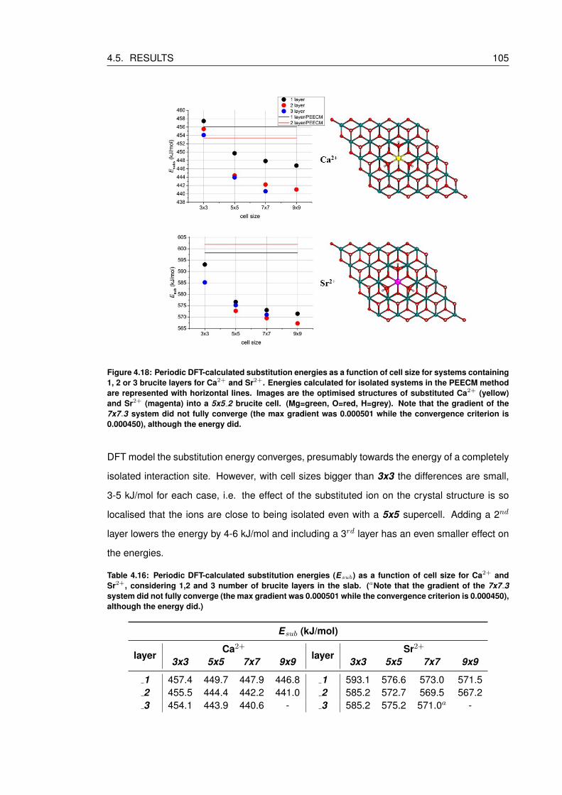
4.5. RESULTS 105
Figure 4.18: Periodic DFT-calculated substitution energies as a function of cell size for systems containing1, 2 or 3 brucite layers for Ca2+ and Sr2+. Energies calculated for isolated systems in the PEECM methodare represented with horizontal lines. Images are the optimised structures of substituted Ca2+ (yellow)and Sr2+ (magenta) into a 5x5 2 brucite cell. (Mg=green, O=red, H=grey). Note that the gradient of the7x7 3 system did not fully converge (the max gradient was 0.000501 while the convergence criterion is0.000450), although the energy did.
DFT model the substitution energy converges, presumably towards the energy of a completely
isolated interaction site. However, with cell sizes bigger than 3x3 the differences are small,
3-5 kJ/mol for each case, i.e. the effect of the substituted ion on the crystal structure is so
localised that the ions are close to being isolated even with a 5x5 supercell. Adding a 2nd
layer lowers the energy by 4-6 kJ/mol and including a 3rd layer has an even smaller effect on
the energies.
Table 4.16: Periodic DFT-calculated substitution energies (Esub) as a function of cell size for Ca2+ andSr2+, considering 1,2 and 3 number of brucite layers in the slab. (aNote that the gradient of the 7x7 3system did not fully converge (the max gradient was 0.000501 while the convergence criterion is 0.000450),although the energy did.)
Esub (kJ/mol)
layerCa2+
layerSr2+
3x3 5x5 7x7 9x9 3x3 5x5 7x7 9x9
1 457.4 449.7 447.9 446.8 1 593.1 576.6 573.0 571.52 455.5 444.4 442.2 441.0 2 585.2 572.7 569.5 567.23 454.1 443.9 440.6 - 3 585.2 575.2 571.0a -
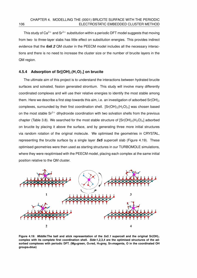
106CHAPTER 4. MODELLING THE (0001) BRUCITE SURFACE WITH THE PERIODIC
ELECTROSTATIC EMBEDDED CLUSTER METHOD
This study of Ca2+ and Sr2+ substitution within a periodic DFT model suggests that moving
from two- to three-layer slabs has little effect on substitution energies. This provides indirect
evidence that the 6x6 2 QM cluster in the PEECM model includes all the necessary interac-
tions and there is no need to increase the cluster size or the number of brucite layers in the
QM region.
4.5.4 Adsorption of Sr[(OH)2(H2O)4] on brucite
The ultimate aim of this project is to understand the interactions between hydrated brucite
surfaces and solvated, fission generated strontium. This study will involve many differently
coordinated complexes and will use their relative energies to identify the most stable among
them. Here we describe a first step towards this aim, i.e. an investigation of adsorbed Sr(OH)2
complexes, surrounded by their first coordination shell. [Sr(OH)2(H2O)4] was chosen based
on the most stable Sr2+ dihydroxide coordination with two solvation shells from the previous
chapter (Table 3.8). We searched for the most stable structure of [Sr(OH)2(H2O)4] adsorbed
on brucite by placing it above the surface, and by generating three more initial structures
via random rotation of the original molecule. We optimised the geometries in CRYSTAL,
representing the brucite surface by a single layer 5x5 supercell slab (Figure 4.19). These
optimised geometries were then used as starting structures in our TURBOMOLE simulations,
where they were reoptimised with the PEECM model, placing each complex at the same initial
position relative to the QM cluster.
Figure 4.19: Middle:The ball and stick representation of the 5x5 1 supercell and the original Sr(OH)2complex with its complete first coordination shell. Side:1,2,3,4 are the optimised structures of the ad-sorbed complexes with periodic DFT. (Mg=green, O=red, H=grey, Sr=magenta, O in the coordinated OHgroups=blue)
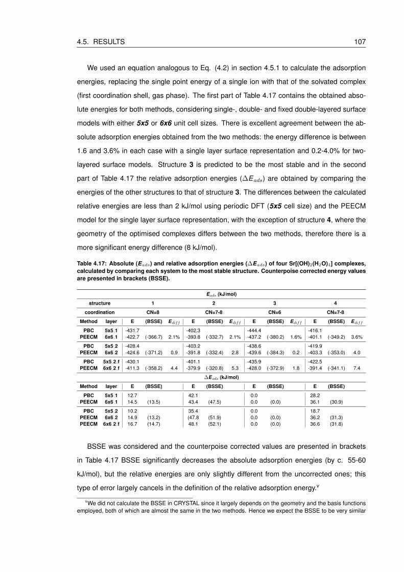
4.5. RESULTS 107
We used an equation analogous to Eq. (4.2) in section 4.5.1 to calculate the adsorption
energies, replacing the single point energy of a single ion with that of the solvated complex
(first coordination shell, gas phase). The first part of Table 4.17 contains the obtained abso-
lute energies for both methods, considering single-, double- and fixed double-layered surface
models with either 5x5 or 6x6 unit cell sizes. There is excellent agreement between the ab-
solute adsorption energies obtained from the two methods: the energy difference is between
1.6 and 3.6% in each case with a single layer surface representation and 0.2-4.0% for two-
layered surface models. Structure 3 is predicted to be the most stable and in the second
part of Table 4.17 the relative adsorption energies (∆Eads) are obtained by comparing the
energies of the other structures to that of structure 3. The differences between the calculated
relative energies are less than 2 kJ/mol using periodic DFT (5x5 cell size) and the PEECM
model for the single layer surface representation, with the exception of structure 4, where the
geometry of the optimised complexes differs between the two methods, therefore there is a
more significant energy difference (8 kJ/mol).
Table 4.17: Absolute (Eads) and relative adsorption energies (∆Eads) of four Sr[(OH)2(H2O)4] complexes,calculated by comparing each system to the most stable structure. Counterpoise corrected energy valuesare presented in brackets (BSSE).
Eads (kJ/mol)
structure 1 2 3 4
coordination CN=8 CN=7-8 CN=6 CN=7-8
Method layer E (BSSE) Ediff E (BSSE) Ediff E (BSSE) Ediff E (BSSE) Ediff
PBC 5x5 1 -431.7 -402.3 -444.4 -416.1PEECM 6x6 1 -422.7 (-366.7) 2.1% -393.8 (-332.7) 2.1% -437.2 (-380.2) 1.6% -401.1 (-349.2) 3.6%
PBC 5x5 2 -428.4 -403.2 -438.6 -419.9PEECM 6x6 2 -424.6 (-371.2) 0.9 -391.8 (-332.4) 2.8 -439.6 (-384.3) 0.2 -403.3 (-353.0) 4.0
PBC 5x5 2 f -430.1 -401.1 -435.9 -422.5PEECM 6x6 2 f -411.3 (-358.2) 4.4 -379.9 (-320.8) 5.3 -428.0 (-372.9) 1.8 -391.4 (-341.1) 7.4
∆Eads (kJ/mol)
Method layer E (BSSE) E (BSSE) E (BSSE) E (BSSE)
PBC 5x5 1 12.7 42.1 0.0 28.2PEECM 6x6 1 14.5 (13.5) 43.4 (47.5) 0.0 (0.0) 36.1 (30.9)
PBC 5x5 2 10.2 35.4 0.0 18.7PEECM 6x6 2 14.9 (13.2) (47.8 (51.9) 0.0 (0.0) 36.2 (31.3)PEECM 6x6 2 f 16.7 (14.7) 48.1 (52.1) 0.0 (0.0) 36.6 (31.8)
BSSE was considered and the counterpoise corrected values are presented in brackets
in Table 4.17 BSSE significantly decreases the absolute adsorption energies (by c. 55-60
kJ/mol), but the relative energies are only slightly different from the uncorrected ones; this
type of error largely cancels in the definition of the relative adsorption energy.v
vWe did not calculate the BSSE in CRYSTAL since it largely depends on the geometry and the basis functionsemployed, both of which are almost the same in the two methods. Hence we expect the BSSE to be very similar

108CHAPTER 4. MODELLING THE (0001) BRUCITE SURFACE WITH THE PERIODIC
ELECTROSTATIC EMBEDDED CLUSTER METHOD
When we consider a two-layer model in the PEECM via a second 6x6 cluster under the first
(6x6 2), the relative adsorption energies are found to be very similar to the single layer results
(6x6 1). Comparing ∆Eads for 5x5 1 and 5x5 2 surface models, there are differences in
relative adsorption energies due to minor structural differences affecting only water molecules
which are not directly coordinated to the Sr2+ ion, but there is no change in terms of either
energetic trends or coordination numbers.
Freezing layers beneath the surface in a slab structure, besides improving the cost effi-
ciency of the calculations, is a common approach to mimic the behaviour of the bulk under-
neath the top layer(s).[57] Although the biggest systems considered in this study contain only
two-layered slabs, we calculated adsorption energies for surface representations in which the
atomic positions in the second brucite layer are fixed to study their possible effects on the
adsorption: 6x6 2 f was already introduced in section 4.4.1, while 5x5 2 f was calculated
by freezing the coordinates of the second layer in the original 5x5 2 cell before its optimisa-
tion. Turning to the periodic DFT results first, the adsorption energies for 5x5 2 f are within
±2 kJ/mol of to the 5x5 2 results, i.e. fixing the atomic positions has no significant effect on
the structures. In the case of the 6x6 2 f PEECM model, Eads is ∼12 kJ/mol higher than
the adsorption energies of 6x6 2. Since comparing the optimised geometries did not reveal
changes in the adsorbed structures, we surmise that this constant energy shift is probably due
to the fact that, in addition to using constraints within the QM cluster, we used the experimental
crystal parameters for the PEECM surface, while the crystal parameters, therefore the original
atomic positions too, were previously optimised for the bulk mineral structure in periodic DFT.
But despite the less accurate crystal structure description in the embedded methods, ∆Eads
values are not affected by changes in the second layer, as shown in Table 4.17: energies for
6x6 2 f are very close to the 6x6 1 and 6x6 2 results.
Changing the cell size for the most stable structure (3) has very small effect on the ad-
sorption energies: comparing the 5x5 1 result to the biggest cell size, 9x9 2, gives an energy
difference of 3.4 kJ/mol. Although we did not consider every cell size for the less stable struc-
tures, the results in Table 4.18 show that increasing the cell size up to 7x7 and 9x9 in periodic
DFT causes a less than 7 kJ/mol energy difference in the absolute adsorption energies for
structure 1,2 and 4. Although the values of the relative adsorption energy change more with
bigger cell sizes compared with the excellent agreement showed for the 5x5 and 6x6 compar-
in the two models. Besides, the relative adsorption energies, in which we are primarily interested, are largelyunaffected by this type of error.

4.5. RESULTS 109
ison in Table 4.17, the energetic trend is not affected (see Table 4.19), which suggests that the
5x5 cell size is reasonable for periodic DFT and indirectly shows that the 6x6 cluster size used
in the PEECM contains all the atoms in the QM region which play a part in the adsorption.
Table 4.18: Periodic DFT-calculated adsorption energies (Eads) as a function of cell size for structure 1-4.A full cell size study was performed for the most stable structure (3) and cell sizes of 7x7 1, 7x7 2 and9x9 1 were calculated for the less stable structures. (aNote that the total energy of structure 2 with 7x7 2cell size converged to 10−5 a.u.)
Eads (kJ/mol)
1 2 3 45x5 7x7 9x9 5x5 7x7 9x9 5x5 7x7 9x9 5x5 7x7 9x9
1 -431.7 -434.1 -435.1 -402.3 -406.8 -408.9 -444.4 -443.5 -444.2 -416.1 -422.0 -418.72 -428.4 -431.4 - -403.2 -406.0a - -438.6 -441.0 -441.0 -419.9 -414.4 -3 - - - - - - -439.1 -441.0 - - - -
2 f -430.1 - - -401.1 - - -435.9 - - -422.5 - -
Table 4.19: Periodic DFT-calculated relative adsorption energies (∆Eads) of four [Sr(OH)2(H2O)4] com-plexes, calculated by comparing each system to the most stable structure (3) with different cell sizes(aNote that the total energy of structure 2 with 7x7 2 cell size converged to 10−5 a.u.)
∆Eads (kJ/mol)
Cell 1 2 3 4
5x5 1 12.7 42.1 0.0 28.25x5 2 10.2 35.4 0.0 18.77x7 1 9.4 36.7 0.0 21.57x7 2 9.6 35.0a 0.0 26.69x9 1 9.2 35.3 0.0 25.5
Overall, this study suggests that including a relaxed or fixed 2nd layer in the surface model
has only minor effects on the relatively weak adsorptions of the hydrated complexes. While
there are some small differences in relative adsorption energies, the energetic trends within
structures 1-4 and the geometries of the coordinated Sr2+ complexes do not change. Re-
sults obtained from periodic DFT and PEECM predict similar structures and have the same
energetic trends.
Assesment of local coordination via the QTAIM
In order to probe further the comparison between the periodic DFT and the PEECM gener-
ated structures, we explored the coordination environment around the Sr2+ ion by examining
the Sr-O distances and by calculating QTAIM bond critical point (BCP) electron densities for
the Sr-O interactions (Table 4.20). The QTAIM is a well-known theory which uses the topology
of the electron density to analyse atomic properties in molecules or complexes (see section
2.7.3.1).[118, 119] Bond critical points are stationary points in the electron density distribution
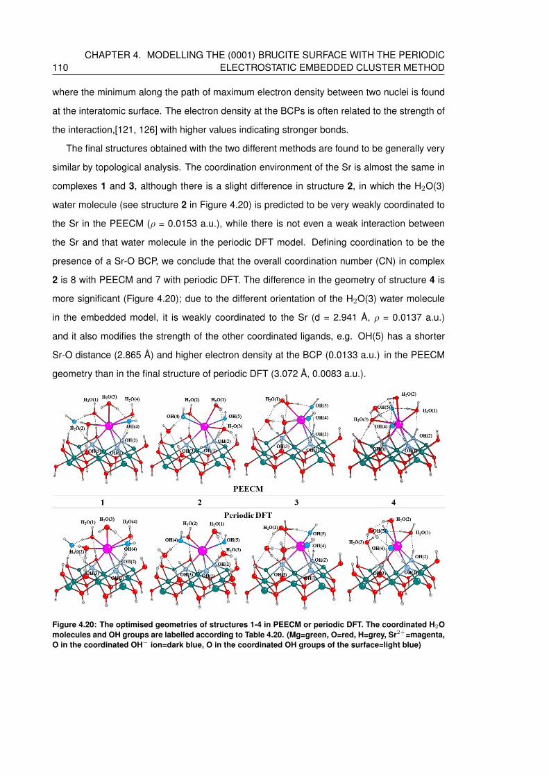
110CHAPTER 4. MODELLING THE (0001) BRUCITE SURFACE WITH THE PERIODIC
ELECTROSTATIC EMBEDDED CLUSTER METHOD
where the minimum along the path of maximum electron density between two nuclei is found
at the interatomic surface. The electron density at the BCPs is often related to the strength of
the interaction,[121, 126] with higher values indicating stronger bonds.
The final structures obtained with the two different methods are found to be generally very
similar by topological analysis. The coordination environment of the Sr is almost the same in
complexes 1 and 3, although there is a slight difference in structure 2, in which the H2O(3)
water molecule (see structure 2 in Figure 4.20) is predicted to be very weakly coordinated to
the Sr in the PEECM (ρ = 0.0153 a.u.), while there is not even a weak interaction between
the Sr and that water molecule in the periodic DFT model. Defining coordination to be the
presence of a Sr-O BCP, we conclude that the overall coordination number (CN) in complex
2 is 8 with PEECM and 7 with periodic DFT. The difference in the geometry of structure 4 is
more significant (Figure 4.20); due to the different orientation of the H2O(3) water molecule
in the embedded model, it is weakly coordinated to the Sr (d = 2.941 A, ρ = 0.0137 a.u.)
and it also modifies the strength of the other coordinated ligands, e.g. OH(5) has a shorter
Sr-O distance (2.865 A) and higher electron density at the BCP (0.0133 a.u.) in the PEECM
geometry than in the final structure of periodic DFT (3.072 A, 0.0083 a.u.).
Figure 4.20: The optimised geometries of structures 1-4 in PEECM or periodic DFT. The coordinated H2Omolecules and OH groups are labelled according to Table 4.20. (Mg=green, O=red, H=grey, Sr2+=magenta,O in the coordinated OH− ion=dark blue, O in the coordinated OH groups of the surface=light blue)
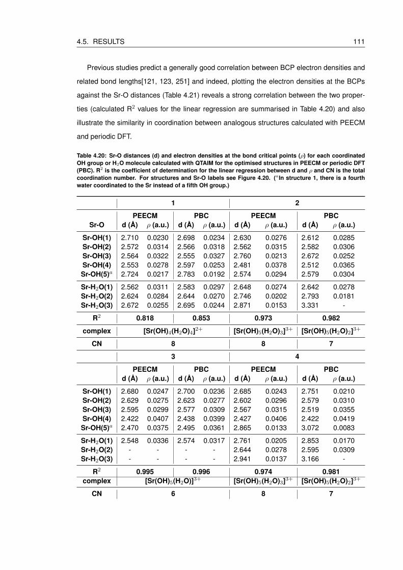
4.5. RESULTS 111
Previous studies predict a generally good correlation between BCP electron densities and
related bond lengths[121, 123, 251] and indeed, plotting the electron densities at the BCPs
against the Sr-O distances (Table 4.21) reveals a strong correlation between the two proper-
ties (calculated R2 values for the linear regression are summarised in Table 4.20) and also
illustrate the similarity in coordination between analogous structures calculated with PEECM
and periodic DFT.
Table 4.20: Sr-O distances (d) and electron densities at the bond critical points (ρ) for each coordinatedOH group or H2O molecule calculated with QTAIM for the optimised structures in PEECM or periodic DFT(PBC). R2 is the coefficient of determination for the linear regression between d and ρ and CN is the totalcoordination number. For structures and Sr-O labels see Figure 4.20. (aIn structure 1, there is a fourthwater coordinated to the Sr instead of a fifth OH group.)
1 2
PEECM PBC PEECM PBCSr-O d (A) ρ (a.u.) d (A) ρ (a.u.) d (A) ρ (a.u.) d (A) ρ (a.u.)
Sr-OH(1) 2.710 0.0230 2.698 0.0234 2.630 0.0276 2.612 0.0285Sr-OH(2) 2.572 0.0314 2.566 0.0318 2.562 0.0315 2.582 0.0306Sr-OH(3) 2.564 0.0322 2.555 0.0327 2.760 0.0213 2.672 0.0252Sr-OH(4) 2.553 0.0278 2.597 0.0253 2.481 0.0378 2.512 0.0365Sr-OH(5)a 2.724 0.0217 2.783 0.0192 2.574 0.0294 2.579 0.0304
Sr-H2O(1) 2.562 0.0311 2.583 0.0297 2.648 0.0274 2.642 0.0278Sr-H2O(2) 2.624 0.0284 2.644 0.0270 2.746 0.0202 2.793 0.0181Sr-H2O(3) 2.672 0.0255 2.695 0.0244 2.871 0.0153 3.331 -
R2 0.818 0.853 0.973 0.982
complex [Sr(OH)4(H2O)4]2+ [Sr(OH)5(H2O)3]3+ [Sr(OH)5(H2O)2]3+
CN 8 8 7
3 4
PEECM PBC PEECM PBCd (A) ρ (a.u.) d (A) ρ (a.u.) d (A) ρ (a.u.) d (A) ρ (a.u.)
Sr-OH(1) 2.680 0.0247 2.700 0.0236 2.685 0.0243 2.751 0.0210Sr-OH(2) 2.629 0.0275 2.623 0.0277 2.602 0.0296 2.579 0.0310Sr-OH(3) 2.595 0.0299 2.577 0.0309 2.567 0.0315 2.519 0.0355Sr-OH(4) 2.422 0.0407 2.438 0.0399 2.427 0.0406 2.422 0.0419Sr-OH(5)a 2.470 0.0375 2.495 0.0361 2.865 0.0133 3.072 0.0083
Sr-H2O(1) 2.548 0.0336 2.574 0.0317 2.761 0.0205 2.853 0.0170Sr-H2O(2) - - - - 2.644 0.0278 2.595 0.0309Sr-H2O(3) - - - - 2.941 0.0137 3.166 -
R2 0.995 0.996 0.974 0.981complex [Sr(OH)5(H2O)]3+ [Sr(OH)5(H2O)3]3+ [Sr(OH)5(H2O)2]3+
CN 6 8 7
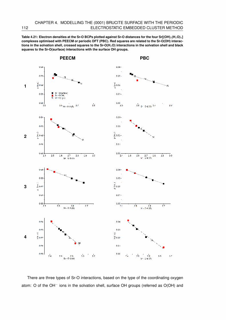
112CHAPTER 4. MODELLING THE (0001) BRUCITE SURFACE WITH THE PERIODIC
ELECTROSTATIC EMBEDDED CLUSTER METHOD
Table 4.21: Electron densities at the Sr-O BCPs plotted against Sr-O distances for the four Sr[(OH)2(H2O)4]complexes optimised with PEECM or periodic DFT (PBC). Red squares are related to the Sr-O(OH) interac-tions in the solvation shell, crossed squares to the Sr-O(H2O) interactions in the solvation shell and blacksquares to the Sr-O(surface) interactions with the surface OH groups.
PEECM PBC
1
2
3
4
There are three types of Sr-O interactions, based on the type of the coordinating oxygen
atom: O of the OH− ions in the solvation shell, surface OH groups (referred as O(OH) and

4.6. CONCLUSIONS 113
O(surface) in the following text) and H2O molecules in the solvation shell (O(H2O)). The ones
expected to have the strongest interaction with the Sr2+ ion are the OH− ions in the solvation
shell. However, this is not always the case, in fact, in structure 1 the only OH− ion directly
coordinating to the Sr is slightly outstanding from the trend, resulting in an R2 value of 0.818
(0.853) with PEECM (periodic DFT). The O(OH) in this case has a weaker interaction ac-
cording to the QTAIM analysis than the Sr-O distance would suggest, but the reason for this
behaviour is unknown. Furthermore, in structure 4, there is a very weakly coordinated O(OH)
in the complex (OH(5)), as opposed to the other OH ion, OH(4), which has the strongest co-
ordination to the Sr ion. In structure 3, which is predicted to be the most stable, the OH− ions
in the solvation shell have the strongest interaction, followed by the only coordinated water
molecule and then the surface OH groups which exhibit the weakest interaction.
4.6 Conclusions
The (0001) brucite surface is one of the most common solid surfaces existing in the nu-
clear sludge. To efficiently study its possible interaction with the Sr2+ ion we were aiming for a
surface model which has a moderate computational cost and is compatible with the solvated
complexes described in the previous chapter. We therefore used the PEECM implemented in
the TURBOMOLE code, which makes this study the first time to model a layered, not purely
ionic surface (brucite (0001) with this method. After the careful development of the PEECM
model, it has been tested in studies related to our final goal, studying the adsorption of ra-
dioactive ions on hydrated brucite surfaces.
The PEECM is capable of describing the adsorption of single s block ions onto brucite,
although the basis set quality has to be carefully considered. At least triple-zeta quality is
necessary to obtain the correct energetic ordering between the ions, but these larger basis
functions must be avoided in the QM representation of the surface cluster, since they can
cause artificial interactions between the boundary atoms and the point charge region.
Combining the results of the s block ion adsorption with the short study of a Sr2+ hy-
drate showed that the calculated adsorption energies slightly depend on the position of the
adsorption site relative to the cluster boundaries and the type of the surface model used.
Fixing more atomic positions always lowers the interaction energy, while introducing a PC
layer underneath the cluster increases the attraction. The two effects combined, results in
slightly more favourable adsorption (6x6 1+PC). Embedding a second layer in the QM cluster
also predicts the adsorption of ions and complexes more favourable (6x6 2) than results in
114CHAPTER 4. MODELLING THE (0001) BRUCITE SURFACE WITH THE PERIODIC
ELECTROSTATIC EMBEDDED CLUSTER METHOD
a single layer. Electron density difference plots suggest that atoms in the second layer are
also involved in the interaction and therefore including the second layer explicitly is preferred
instead the addition of a PC layer.
Through a comparison with periodic DFT, we have demonstrated that the PEECM suffi-
ciently reflects the qualities of the brucite surface to be able to describe both the substitution
of Ca2+ or Sr2+ into brucite and the surface complexation of [Sr(OH)2(H2O)4]. Based on the
cell size studies and the interaction energies obtained with multiple layers of brucite, the size
of the quantum chemically treated cluster is found to be reasonable in all cases. The agree-
ment between adsorption energies and the optimised geometries obtained with PEECM or
periodic DFT is excellent in the case of the adsorption of [Sr(OH)2(H2O)4] complexes.
These results give us confidence to step forward and use the embedded brucite (0001)
model in future investigations of Sr2+ complex ion adsorptions on hydrated surfaces. They
demonstrate that the PEECM is capable of describing sorption mechanisms on brucite-like
surfaces, and that the approach is a viable alternative to periodic DFT when ionic species are
involved in surface interactions. Furthermore, we note that there is a significant difference in
computational speed between the two methods: if we consider structure 1 in section 4.5.4
as a test system, one optimisation step with a 5x5 1 cell in periodic DFT took an average 15
minutes using 192 cores; while the same structure on a 6x6 1 cluster did an average 1 optimi-
sation step in 15 minutes using 10 cores with the PEECM. The embedded cluster calculations
presented here were run largely on our local departmental compute server, with a modest
number of cores per calculation, by contrast to the periodic DFT calculations, which required
the massively parallel version of the CRYSTAL code and were run on the UK’s national su-
percomputing facility. This difference in computational requirements makes the application of
PEECM especially relevant in case of industry related problems.
Moving on to more realistic models of the hydrated surface, we extended our PEECM
study to include many more water molecules in the QM region, allowing to probe effects of
second shell water molecules on the adsorption. The results of this study are presented in the
following chapter.
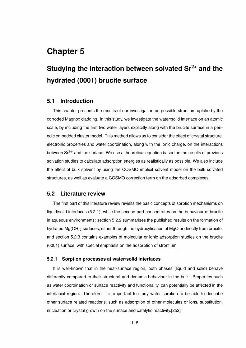
Chapter 5
Studying the interaction between solvated Sr2+ and the
hydrated (0001) brucite surface
5.1 Introduction
This chapter presents the results of our investigation on possible strontium uptake by the
corroded Magnox cladding. In this study, we investigate the water/solid interface on an atomic
scale, by including the first two water layers explicitly along with the brucite surface in a peri-
odic embedded cluster model. This method allows us to consider the effect of crystal structure,
electronic properties and water coordination, along with the ionic charge, on the interactions
between Sr2+ and the surface. We use a theoretical equation based on the results of previous
solvation studies to calculate adsorption energies as realistically as possible. We also include
the effect of bulk solvent by using the COSMO implicit solvent model on the bulk solvated
structures, as well as evaluate a COSMO correction term on the adsorbed complexes.
5.2 Literature review
The first part of this literature review revisits the basic concepts of sorption mechanisms on
liquid/solid interfaces (5.2.1), while the second part concentrates on the behaviour of brucite
in aqueous environments: section 5.2.2 summarises the published results on the formation of
hydrated Mg(OH)2 surfaces, either through the hydroxylisation of MgO or directly from brucite,
and section 5.2.3 contains examples of molecular or ionic adsorption studies on the brucite
(0001) surface, with special emphasis on the adsorption of strontium.
5.2.1 Sorption processes at water/solid interfaces
It is well-known that in the near-surface region, both phases (liquid and solid) behave
differently compared to their structural and dynamic behaviour in the bulk. Properties such
as water coordination or surface reactivity and functionality, can potentially be affected in the
interfacial region. Therefore, it is important to study water sorption to be able to describe
other surface related reactions, such as adsorption of other molecules or ions, substitution,
nucleation or crystal growth on the surface and catalytic reactivity.[252]
115
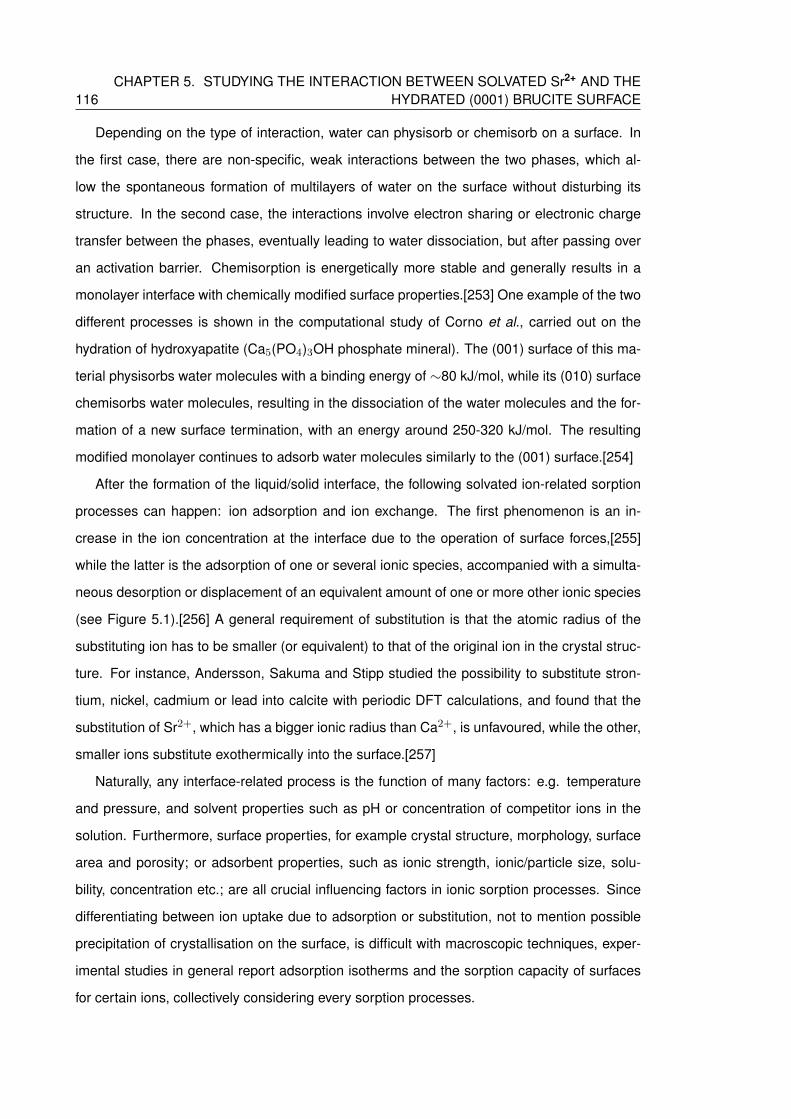
116CHAPTER 5. STUDYING THE INTERACTION BETWEEN SOLVATED Sr2+ AND THE
HYDRATED (0001) BRUCITE SURFACE
Depending on the type of interaction, water can physisorb or chemisorb on a surface. In
the first case, there are non-specific, weak interactions between the two phases, which al-
low the spontaneous formation of multilayers of water on the surface without disturbing its
structure. In the second case, the interactions involve electron sharing or electronic charge
transfer between the phases, eventually leading to water dissociation, but after passing over
an activation barrier. Chemisorption is energetically more stable and generally results in a
monolayer interface with chemically modified surface properties.[253] One example of the two
different processes is shown in the computational study of Corno et al., carried out on the
hydration of hydroxyapatite (Ca5(PO4)3OH phosphate mineral). The (001) surface of this ma-
terial physisorbs water molecules with a binding energy of ∼80 kJ/mol, while its (010) surface
chemisorbs water molecules, resulting in the dissociation of the water molecules and the for-
mation of a new surface termination, with an energy around 250-320 kJ/mol. The resulting
modified monolayer continues to adsorb water molecules similarly to the (001) surface.[254]
After the formation of the liquid/solid interface, the following solvated ion-related sorption
processes can happen: ion adsorption and ion exchange. The first phenomenon is an in-
crease in the ion concentration at the interface due to the operation of surface forces,[255]
while the latter is the adsorption of one or several ionic species, accompanied with a simulta-
neous desorption or displacement of an equivalent amount of one or more other ionic species
(see Figure 5.1).[256] A general requirement of substitution is that the atomic radius of the
substituting ion has to be smaller (or equivalent) to that of the original ion in the crystal struc-
ture. For instance, Andersson, Sakuma and Stipp studied the possibility to substitute stron-
tium, nickel, cadmium or lead into calcite with periodic DFT calculations, and found that the
substitution of Sr2+, which has a bigger ionic radius than Ca2+, is unfavoured, while the other,
smaller ions substitute exothermically into the surface.[257]
Naturally, any interface-related process is the function of many factors: e.g. temperature
and pressure, and solvent properties such as pH or concentration of competitor ions in the
solution. Furthermore, surface properties, for example crystal structure, morphology, surface
area and porosity; or adsorbent properties, such as ionic strength, ionic/particle size, solu-
bility, concentration etc.; are all crucial influencing factors in ionic sorption processes. Since
differentiating between ion uptake due to adsorption or substitution, not to mention possible
precipitation of crystallisation on the surface, is difficult with macroscopic techniques, exper-
imental studies in general report adsorption isotherms and the sorption capacity of surfaces
for certain ions, collectively considering every sorption processes.
5.2. LITERATURE REVIEW 117
Figure 5.1: Schematic representation of adsorption and ion substitution at liquid/solid interfaces
5.2.2 Hydration of MgO and Mg(OH)2 surfaces
The behaviour of interfacial water on MgO (periclase) and Mg(OH)2 (brucite) surfaces has
been extensively studied with both experimental[258–268] and theoretical methods[261, 269–
280]. Magnesium-oxide is important for this study, because brucite is the most common al-
teration producti of periclase in nature.[281] Although the (001) surface of MgO is known to
be the most stable and the hydroxylation of a perfect (001) surface is predicted to be un-
favoured,[272–274] experimental results show that, MgO is generally highly defective[262–
264, 269] and there are hydroxyl groups on its surface in aqueous media.[258–260] The water
chemisorbs on the low-coordinated defect sites,[269, 274, 276] such as the 4-fold-coordinated
edges[275] or 3-fold-coordinated corners, and forms OH surface groups, eventually turning the
surface to (0001) brucite.[261, 265]
In fact, Refson et al.[275] computationally showed that, instead of the (001) MgO surface,
the otherwise metastable (111) phase is the most stable in aqueous solution, which can easily
be hydroxylated and transformed to (0001) brucite (see Figure 5.2). When the possible ad-
sorption sites at the MgO surfaces are fully protonated, additional water starts to physisorb on
the (0001) surface of the Mg(OH)2.
Depending on the surrounding conditions, the formation of Mg(OH)2 from periclase can be
reversible; with water removal, brucite decomposes via a dehydroxylation process: Mg(OH)2
−→ MgO + H2O.[282] Early experimental studies of water vapour adsorption on brucite un-
der vacuum, show that during the hydration-dehydration cycles the surface ages quickly, i.e.
it decomposes to MgO with the removal of the water molecules.[266, 267, 282] However,
iMineral alteration refers to natural chemical or mineralogical processes which change the chemical composi-tion of the mineral.
118CHAPTER 5. STUDYING THE INTERACTION BETWEEN SOLVATED Sr2+ AND THE
HYDRATED (0001) BRUCITE SURFACE
Figure 5.2: Side view of the (a) hypothetical hydroxylated (001) surface of MgO, (b) (0001) surface ofMg(OH)2 and (c) hydroxylated (111) surface of MgO [275]
the equilibrium of this reaction is strongly related to the vapor pressure and under ambient
conditions the dehydroxylation is unlikely to happen (the reaction starts at 275°C under 1
bar).[283, 284] Ab initio studies on the decomposition of Mg(OH)2 were carried out to identify
the most reactive surface sites for the reaction[229, 230] and by comparing the dehydroxyla-
tion energies at the different brucite surfaces, they suggest that the reaction starts at (1100)
surface.[230]
The behaviour of brucite under ambient conditions in aqueous phase, depending on the pH
conditions, the surface can be protonated or deprotontated which also affects the dissolution
rate of the mineral. According to electrophoretic measurements[285] and the experimental
work of Pokrovsky et al.[268], the isoelectric point (pHIEP ) of brucite is close to pH 11; and
the net surface charge is positive under this point and negative above it (see Figure 5.3).
By investigating the surface speciation of brucite at different pH, Pokrovsky and Schott
found that the dominant species below pH 8 are >MgOH+2 ,ii formed by the protonation of the
OH surface groups, while the concentration of the deprotonated >MgO− species becomes
significant only above pH 12, although the neutral >MgOH0 species are still favoured, see
Figure 5.3. The increased concentration of protonated species with decreasing pH, results
in an increase in the dissolution rate of the mineral, suggesting that the protonation of the
surface OH group helps to initiate the dissociation reaction.[268, 286]
Although protonation/deprotonation reactions can occur on the surface, force field based
molecular dynamic studies[277–280] have to assume conditions near to the zero point of net
proton charge, because simulating bond breaking or bond formation is not possible with this
method.[279] Despite the lack of possible protonation, classical MD calculations still provide
crucial information about the effect of the vicinity of the surface on the behaviour of interfacial
iiThe notation ”>” refers to the fact that the following chemical formula (MgOH+2 ) describes a surface specimen,
i.e. it is related to one Mg-OH group.
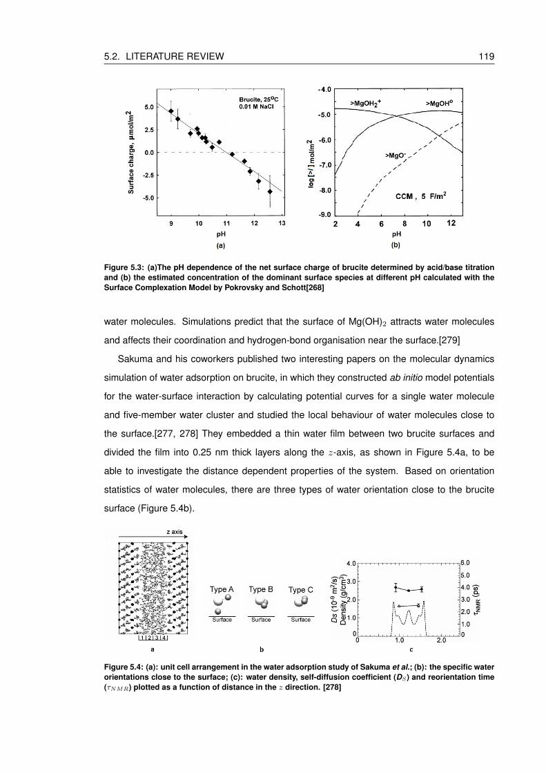
5.2. LITERATURE REVIEW 119
Figure 5.3: (a)The pH dependence of the net surface charge of brucite determined by acid/base titrationand (b) the estimated concentration of the dominant surface species at different pH calculated with theSurface Complexation Model by Pokrovsky and Schott[268]
water molecules. Simulations predict that the surface of Mg(OH)2 attracts water molecules
and affects their coordination and hydrogen-bond organisation near the surface.[279]
Sakuma and his coworkers published two interesting papers on the molecular dynamics
simulation of water adsorption on brucite, in which they constructed ab initio model potentials
for the water-surface interaction by calculating potential curves for a single water molecule
and five-member water cluster and studied the local behaviour of water molecules close to
the surface.[277, 278] They embedded a thin water film between two brucite surfaces and
divided the film into 0.25 nm thick layers along the z-axis, as shown in Figure 5.4a, to be
able to investigate the distance dependent properties of the system. Based on orientation
statistics of water molecules, there are three types of water orientation close to the brucite
surface (Figure 5.4b).
Figure 5.4: (a): unit cell arrangement in the water adsorption study of Sakuma et al.; (b): the specific waterorientations close to the surface; (c): water density, self-diffusion coefficient (DS) and reorientation time(τNMR) plotted as a function of distance in the z direction. [278]

120CHAPTER 5. STUDYING THE INTERACTION BETWEEN SOLVATED Sr2+ AND THE
HYDRATED (0001) BRUCITE SURFACE
Type A is the most common, and is connected to the surface hydroxyl groups via a hydrogen-
bond, formed between one of its protons and the oxygen of the down-facing OH groups of the
top layer. But Sakuma et al. note that based on the potential energy curves that they cal-
culated and compared to the potential of a water-water interaction, the hydrogen-bonding
between the water molecules and the surface is weaker than the hydrogen-bonds between
water molecules. Type C is a less frequent coordination mode which makes connections with
the surface via its oxygen. Type B makes hydrogen-bonds only with type A and C molecules.
Sakuma and coworkers also calculated solution properties, such as the density, self-
diffusion coefficient and reorientation time, shown as a function of the distance along the z
axis in Figure 5.4c.[277, 278] The density of the water molecules is significantly higher in wa-
ter layers close to the surface. The two highest peaks on the symmetrical density diagram
are related mainly to water molecules with type A orientation, and the shoulders correspond
to type C. The second biggest peak in the middle has no specific orientation and it represents
the density in the middle of the water film. Besides the density distribution, they evaluated the
self-diffusion coefficient (DS) and the reorientation time (τNMR). Surprisingly, they found a
larger DS and a smaller τNMR close to the surfaces, which is anomalous,[279] if we consider
that bound water molecules are less likely to change coordination in a short time, and their
results indicate that the water molecules next to the surface can move and rotate faster than
in the bulk.
Wang et al. carried out a similar MD study on the water/brucite interface, but looking at
different pore sizes, by representing them with a series of water films with different thicknesses
between the brucite layers.[279] Their results show that under a pore size of 12 A, all water
molecules are affected by the presence of the brucite, but above 12 A, the middle of the water
film has similar properties to the bulk aqueous phase. They also studied the structure of the
first two water layers and they found that they are on average 2.40 A and 4.95 A away from
the surface,[280] and the water molecules within them have limited positions and orientations,
very similar to the A, B and C positions which were identified by Sakuma et al. They also
predicted that the A structure is more likely to appear, with a 5/4 ratio between A and C.
Interestingly, they also found a small fraction of water molecules to be coordinated to the
surface via two hydrogen bonds with their two H atoms. They suggest that this indicates a
possible proton transfer between the water molecules and surface OH groups which cannot
be addressed by classical MD.[279]
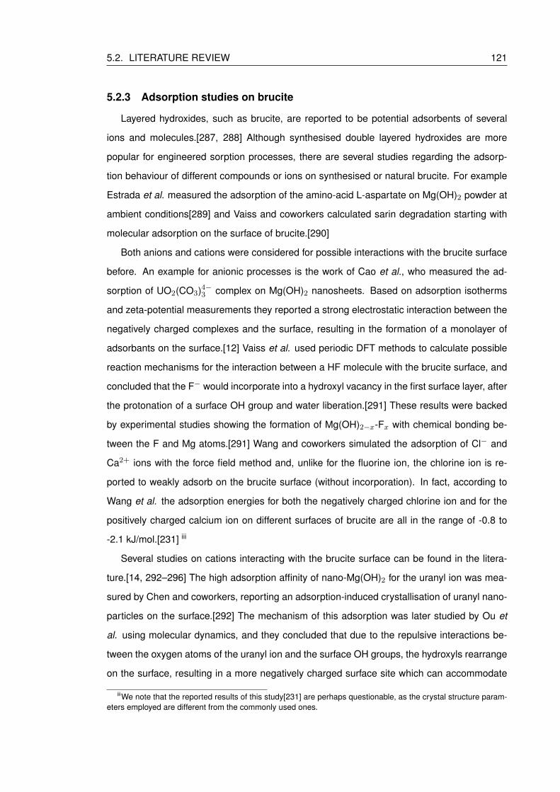
5.2. LITERATURE REVIEW 121
5.2.3 Adsorption studies on brucite
Layered hydroxides, such as brucite, are reported to be potential adsorbents of several
ions and molecules.[287, 288] Although synthesised double layered hydroxides are more
popular for engineered sorption processes, there are several studies regarding the adsorp-
tion behaviour of different compounds or ions on synthesised or natural brucite. For example
Estrada et al. measured the adsorption of the amino-acid L-aspartate on Mg(OH)2 powder at
ambient conditions[289] and Vaiss and coworkers calculated sarin degradation starting with
molecular adsorption on the surface of brucite.[290]
Both anions and cations were considered for possible interactions with the brucite surface
before. An example for anionic processes is the work of Cao et al., who measured the ad-
sorption of UO2(CO3)4−3 complex on Mg(OH)2 nanosheets. Based on adsorption isotherms
and zeta-potential measurements they reported a strong electrostatic interaction between the
negatively charged complexes and the surface, resulting in the formation of a monolayer of
adsorbants on the surface.[12] Vaiss et al. used periodic DFT methods to calculate possible
reaction mechanisms for the interaction between a HF molecule with the brucite surface, and
concluded that the F− would incorporate into a hydroxyl vacancy in the first surface layer, after
the protonation of a surface OH group and water liberation.[291] These results were backed
by experimental studies showing the formation of Mg(OH)2−x-Fx with chemical bonding be-
tween the F and Mg atoms.[291] Wang and coworkers simulated the adsorption of Cl− and
Ca2+ ions with the force field method and, unlike for the fluorine ion, the chlorine ion is re-
ported to weakly adsorb on the brucite surface (without incorporation). In fact, according to
Wang et al. the adsorption energies for both the negatively charged chlorine ion and for the
positively charged calcium ion on different surfaces of brucite are all in the range of -0.8 to
-2.1 kJ/mol.[231] iii
Several studies on cations interacting with the brucite surface can be found in the litera-
ture.[14, 292–296] The high adsorption affinity of nano-Mg(OH)2 for the uranyl ion was mea-
sured by Chen and coworkers, reporting an adsorption-induced crystallisation of uranyl nano-
particles on the surface.[292] The mechanism of this adsorption was later studied by Ou et
al. using molecular dynamics, and they concluded that due to the repulsive interactions be-
tween the oxygen atoms of the uranyl ion and the surface OH groups, the hydroxyls rearrange
on the surface, resulting in a more negatively charged surface site which can accommodate
iiiWe note that the reported results of this study[231] are perhaps questionable, as the crystal structure param-eters employed are different from the commonly used ones.
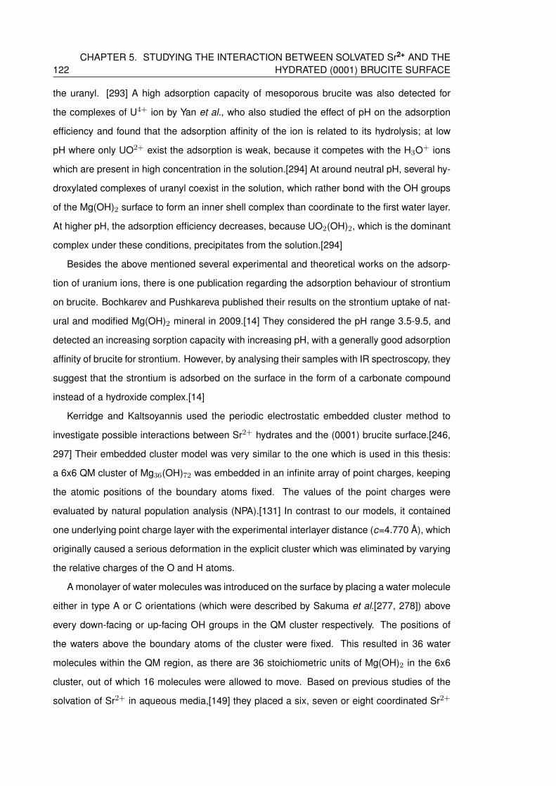
122CHAPTER 5. STUDYING THE INTERACTION BETWEEN SOLVATED Sr2+ AND THE
HYDRATED (0001) BRUCITE SURFACE
the uranyl. [293] A high adsorption capacity of mesoporous brucite was also detected for
the complexes of U4+ ion by Yan et al., who also studied the effect of pH on the adsorption
efficiency and found that the adsorption affinity of the ion is related to its hydrolysis; at low
pH where only UO2+ exist the adsorption is weak, because it competes with the H3O+ ions
which are present in high concentration in the solution.[294] At around neutral pH, several hy-
droxylated complexes of uranyl coexist in the solution, which rather bond with the OH groups
of the Mg(OH)2 surface to form an inner shell complex than coordinate to the first water layer.
At higher pH, the adsorption efficiency decreases, because UO2(OH)2, which is the dominant
complex under these conditions, precipitates from the solution.[294]
Besides the above mentioned several experimental and theoretical works on the adsorp-
tion of uranium ions, there is one publication regarding the adsorption behaviour of strontium
on brucite. Bochkarev and Pushkareva published their results on the strontium uptake of nat-
ural and modified Mg(OH)2 mineral in 2009.[14] They considered the pH range 3.5-9.5, and
detected an increasing sorption capacity with increasing pH, with a generally good adsorption
affinity of brucite for strontium. However, by analysing their samples with IR spectroscopy, they
suggest that the strontium is adsorbed on the surface in the form of a carbonate compound
instead of a hydroxide complex.[14]
Kerridge and Kaltsoyannis used the periodic electrostatic embedded cluster method to
investigate possible interactions between Sr2+ hydrates and the (0001) brucite surface.[246,
297] Their embedded cluster model was very similar to the one which is used in this thesis:
a 6x6 QM cluster of Mg36(OH)72 was embedded in an infinite array of point charges, keeping
the atomic positions of the boundary atoms fixed. The values of the point charges were
evaluated by natural population analysis (NPA).[131] In contrast to our models, it contained
one underlying point charge layer with the experimental interlayer distance (c=4.770 A), which
originally caused a serious deformation in the explicit cluster which was eliminated by varying
the relative charges of the O and H atoms.
A monolayer of water molecules was introduced on the surface by placing a water molecule
either in type A or C orientations (which were described by Sakuma et al.[277, 278]) above
every down-facing or up-facing OH groups in the QM cluster respectively. The positions of
the waters above the boundary atoms of the cluster were fixed. This resulted in 36 water
molecules within the QM region, as there are 36 stoichiometric units of Mg(OH)2 in the 6x6
cluster, out of which 16 molecules were allowed to move. Based on previous studies of the
solvation of Sr2+ in aqueous media,[149] they placed a six, seven or eight coordinated Sr2+
5.3. COMPUTATIONAL DETAILS 123
hydrate at different distances from the brucite surface and optimised the structure. Based on
these results, they identified three coordination regimes, as shown in Figure 5.5: an inner
shell (r < 4 A) where the Sr2+ is directly coordinated to the OH groups on the surface; an
outer shell (4 < r < 6 A) where the complex is coordinated to the monolayer of water on the
surface; and an uncoordinated regime (r > 6 A). Based on the relative energies of the studied
systems, they found the coordinated complexes (inner or outer shell ones) to be ∼40 kJ/mol
more stable than the uncoordinated ones.[246]
Figure 5.5: The three coordination regimes of the Sr2+ hydrates on brucite. The surface and the monolayerof water are represented by wires and the complex by balls and sticks.(Sr=gold, O=red, H=white)[246]
The study reported in this chapter is strongly related to the studies of Kerridge and Kaltsoy-
annis; by continuing to use the same approaches, this work extends the existing with model
with more explicit water molecules above the surface and a COSMO-based correction term to
account for the effect of bulk solvent above the hydrated surface. The possible adsorption of
both Sr2+ hydrate and hydroxide complexes are investigated, concentrating on possible links
between coordination structure, the number of solvated OH− ions or Sr-surface distance and
the adsorption energies.
5.3 Computational details
The general computational details are identical to the ones used in chapter 3 and 4 sec-
tion 4.4.1: all calculations were performed with version 6.6 of the TURBOMOLE program[137]
using resolution-of-the-identity density functional theory[180] and the results were visualised
with the MOLDRAW chemical graphical software.[184] The TPSS exchange-correlation func-
tional[77] was used together with the def2-SVP basis sets of polarised double-ζ quality[87,
96] and the associated Sr effective core potential (def2-ecp), which replaces the electrons
occupying the 1s-3d orbitals. The periodic electrostatic embedded cluster method (2.6.2) was
employed throughout this study, using the 6x6 1 (a stoichiometric 6 by 6 Mg atom unit cell)
and 6x6 2 f slabs, introduced in section 4.4.1, to represent the brucite surface. The point
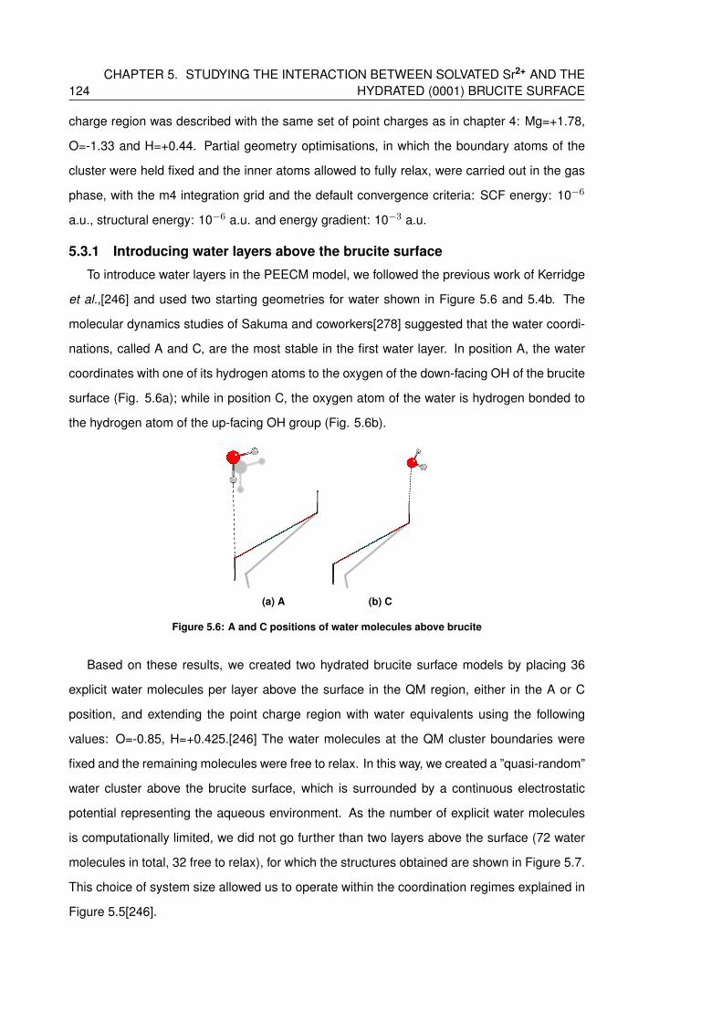
124CHAPTER 5. STUDYING THE INTERACTION BETWEEN SOLVATED Sr2+ AND THE
HYDRATED (0001) BRUCITE SURFACE
charge region was described with the same set of point charges as in chapter 4: Mg=+1.78,
O=-1.33 and H=+0.44. Partial geometry optimisations, in which the boundary atoms of the
cluster were held fixed and the inner atoms allowed to fully relax, were carried out in the gas
phase, with the m4 integration grid and the default convergence criteria: SCF energy: 10−6
a.u., structural energy: 10−6 a.u. and energy gradient: 10−3 a.u.
5.3.1 Introducing water layers above the brucite surface
To introduce water layers in the PEECM model, we followed the previous work of Kerridge
et al.,[246] and used two starting geometries for water shown in Figure 5.6 and 5.4b. The
molecular dynamics studies of Sakuma and coworkers[278] suggested that the water coordi-
nations, called A and C, are the most stable in the first water layer. In position A, the water
coordinates with one of its hydrogen atoms to the oxygen of the down-facing OH of the brucite
surface (Fig. 5.6a); while in position C, the oxygen atom of the water is hydrogen bonded to
the hydrogen atom of the up-facing OH group (Fig. 5.6b).
(a) A (b) C
Figure 5.6: A and C positions of water molecules above brucite
Based on these results, we created two hydrated brucite surface models by placing 36
explicit water molecules per layer above the surface in the QM region, either in the A or C
position, and extending the point charge region with water equivalents using the following
values: O=-0.85, H=+0.425.[246] The water molecules at the QM cluster boundaries were
fixed and the remaining molecules were free to relax. In this way, we created a ”quasi-random”
water cluster above the brucite surface, which is surrounded by a continuous electrostatic
potential representing the aqueous environment. As the number of explicit water molecules
is computationally limited, we did not go further than two layers above the surface (72 water
molecules in total, 32 free to relax), for which the structures obtained are shown in Figure 5.7.
This choice of system size allowed us to operate within the coordination regimes explained in
Figure 5.5[246].
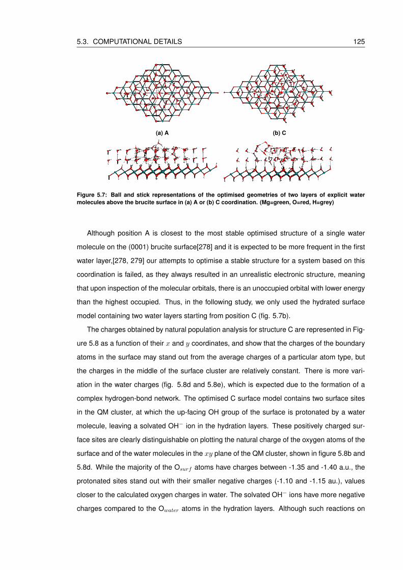
5.3. COMPUTATIONAL DETAILS 125
(a) A (b) C
Figure 5.7: Ball and stick representations of the optimised geometries of two layers of explicit watermolecules above the brucite surface in (a) A or (b) C coordination. (Mg=green, O=red, H=grey)
Although position A is closest to the most stable optimised structure of a single water
molecule on the (0001) brucite surface[278] and it is expected to be more frequent in the first
water layer,[278, 279] our attempts to optimise a stable structure for a system based on this
coordination is failed, as they always resulted in an unrealistic electronic structure, meaning
that upon inspection of the molecular orbitals, there is an unoccupied orbital with lower energy
than the highest occupied. Thus, in the following study, we only used the hydrated surface
model containing two water layers starting from position C (fig. 5.7b).
The charges obtained by natural population analysis for structure C are represented in Fig-
ure 5.8 as a function of their x and y coordinates, and show that the charges of the boundary
atoms in the surface may stand out from the average charges of a particular atom type, but
the charges in the middle of the surface cluster are relatively constant. There is more vari-
ation in the water charges (fig. 5.8d and 5.8e), which is expected due to the formation of a
complex hydrogen-bond network. The optimised C surface model contains two surface sites
in the QM cluster, at which the up-facing OH group of the surface is protonated by a water
molecule, leaving a solvated OH− ion in the hydration layers. These positively charged sur-
face sites are clearly distinguishable on plotting the natural charge of the oxygen atoms of the
surface and of the water molecules in the xy plane of the QM cluster, shown in figure 5.8b and
5.8d. While the majority of the Osurf atoms have charges between -1.35 and -1.40 a.u., the
protonated sites stand out with their smaller negative charges (-1.10 and -1.15 au.), values
closer to the calculated oxygen charges in water. The solvated OH− ions have more negative
charges compared to the Owater atoms in the hydration layers. Although such reactions on
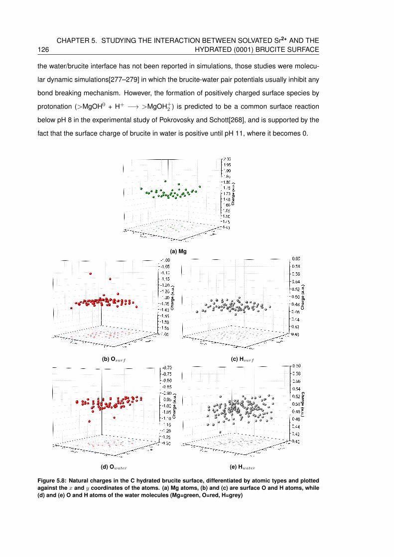
126CHAPTER 5. STUDYING THE INTERACTION BETWEEN SOLVATED Sr2+ AND THE
HYDRATED (0001) BRUCITE SURFACE
the water/brucite interface has not been reported in simulations, those studies were molecu-
lar dynamic simulations[277–279] in which the brucite-water pair potentials usually inhibit any
bond breaking mechanism. However, the formation of positively charged surface species by
protonation (>MgOH0 + H+ −→ >MgOH+2 ) is predicted to be a common surface reaction
below pH 8 in the experimental study of Pokrovosky and Schott[268], and is supported by the
fact that the surface charge of brucite in water is positive until pH 11, where it becomes 0.
(a) Mg
(b) Osurf (c) Hsurf
(d) Owater (e) Hwater
Figure 5.8: Natural charges in the C hydrated brucite surface, differentiated by atomic types and plottedagainst the x and y coordinates of the atoms. (a) Mg atoms, (b) and (c) are surface O and H atoms, while(d) and (e) O and H atoms of the water molecules (Mg=green, O=red, H=grey)
5.4. RESULTS 127
The good agreement with the experimental findings in neutral conditions gave us the con-
fidence to continue with the developed hydrated surface model and introduce Sr complexes
above it. In the results section we investigate the adsorption behaviour of Sr2+ hydrates and
hydroxide complexes on the hydrated brucite (0001) surface.
5.4 Results
The first two sections (5.4.1 and 5.4.2) contain the description of the optimised complexes
obtained for systems with 0, 1 and 2 OH− ions (called group C, C OH1 and C OH2 respec-
tively), while the following sections describe the analysis of the effects of different properties
on the adsorption, such as the Sr-surface distance (5.4.3.1), the number of solvated OH− ions
(5.4.3.2) or the total coordination number.
By applying the previously introduced hydrated brucite surface including 2 water layers
(5.7b), we generated a series of structures in the following way: first, we modelled the ad-
sorption of two Sr2+ hydrate and two hydroxide complexes in group C and C OH2 by placing
a cation at the same position on the xy plane (middle of the cluster) but at varying distances
in the z direction, and optimised the geometry of the whole systems. Then, we modified
these optimised structures by protonating the solvated hydroxide ions or deprotonating wa-
ter molecules to create more initial geometries for the other group. Moreover, structures in
C OH1 were all calculated based on previously optimised hydrate and hydroxide complexes,
and thus they are discussed after the results of the C OH2 groups in section 5.4.2. The
following labelling scheme is employed for the obtained structures:
[Sr : a : b : c](2−b)+ (5.1)
where a, b and c represent the number of water molecules, solvated OH− ions and surface
OH groups coordinated to the cation respectively. For instance, the [Sr:3:0:3]2+ hydrate com-
plex has a total coordination number of six and is directly coordinated to the surface through 3
OH groups with 3 water molecules in its first solvation shell. To decide if a particular molecule
is coordinated to the ion or not, we arbitrarily used the ranges of Sr-ligand distances obtained
in section 4.5.4. If an oxygen atom is further from the Sr than the largest ion-ligand distance
calculated via AIM in that section (d(Sr-O(surf)) > 2.760 A, d(Sr-O(OH)) > 2.865 A, d(Sr-
O(H2O)) > 2.940 A, see Table 4.20), it is considered not coordinated to the cation.
To describe the Sr-surface interactions as realistically as possible, we created a theoretical

128CHAPTER 5. STUDYING THE INTERACTION BETWEEN SOLVATED Sr2+ AND THE
HYDRATED (0001) BRUCITE SURFACE
reaction in which we compare the energy of the adsorbed ion with the energy of a solvated one
in the W24 water cluster, i.e. we look at the propensity of the Sr2+ ion to coordinate with the
surface (inner complex) or with its first hydration layer (outer complex) rather than remaining in
the aqueous phase. We used our previous results obtained in chapter 3 to represent the most
stable structures in solution and calculated the interaction energy with the following equation:
Eads = (Ecomplex + EW24)− (Ehydrated brucite + EW24 complex) (5.2)
Ecomplex is the SCF energy of the adsorbed complex on the hydrated surface, while EW24
is the energy of a 24 water molecule cluster representing the bulk water phase (fig. 3.5).
Ehydrated brucite is the energy of the hydrated brucite surface without the Sr2+ ion (fig. 5.7b).iv
Since we are looking at the adsorption of different types of Sr2+ complexes, the reference sys-
tem used for EW24 complex changes accordingly: for systems in section 5.4.1 [Sr:6/18:0/0]2+
from fig. 3.6a is used, while for systems containing one or two solvated OH− ions in section
5.4.2, the [Sr:5/18:1/0]+ and [Sr:5/17:1/1] hydroxide complexes are employed from table 3.8.
It is important to note, that the chosen reference structures are optimised and predicted
to be the most stable with the use of an implicit solvent model. As it was shown in chapter
3, applying the COSMO model can have significant effect on the energetic stability and the
structure, but its use is not straightforward when an other embedding approach (PEECM)
is employed. Therefore, for initial comparison the SCF energies of EW24 and EW24 complex
were obtained by single point calculations of the most stable structures obtained with the
COSMO method in gas phase using the TPSS/def2-SVP functional-basis set pair. These gas
phase energies were used to calculate the relative adsorption energies of adsorbed structures
as they are summarised in sections 5.4.1 and 5.4.2. The evaluation of absolute adsorption
energies with and without COSMO correction terms is described in more details in section
5.4.3.2.
5.4.1 Adsorption of Sr2+ on a hydrated brucite surface
In this section we present the structure of Sr2+ complexes obtained for a hydrated brucite
surface without solvated hydroxide ions, shown in Figure 5.10 and summarised in Table 5.1.
C1 and C3 complexes were optimised by placing the Sr2+ ion above the hydrated 6x6 1
ivThe Ehydrated brucite term is always the optimised C hydration model of a protonated surface, i.e. representsthe surface in a pH below 11 conditions. Attempts to optimise unprotonated surfaces with the introduction ofsolvated OH− ions within the hydrated surface model, failed due to the difficulties arising from the total negativecharge of the QM cluster.
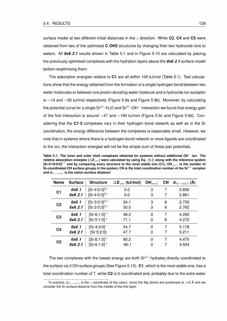
5.4. RESULTS 129
surface model at two different initial distances in the z direction. While C2, C4 and C5 were
obtained from two of the optimised C OH2 structures by changing their two hydroxide ions to
waters. All 6x6 2 f results shown in Table 5.1 and in Figure 5.10 are calculated by placing
the previously optimised complexes with the hydration layers above the 6x6 2 f surface model
before reoptimising them.
The adsorption energies relative to C1 are all within 100 kJ/mol (Table 5.1). Test calcula-
tions show that the energy obtained from the formation of a single hydrogen bond between two
water molecules or between one proton donating water molecule and a hydroxide ion acceptor
is ∼14 and ∼50 kJ/mol respectively (Figure 5.9a and Figure 5.9b). Moreover, by calculating
the potential curve for a single Sr2+-H2O and Sr2+-OH− interaction we found that energy gain
of the first interaction is around ∼47 and ∼160 kJ/mol (Figure 5.9c and Figure 5.9d). Con-
sidering that the C1-5 complexes vary in their hydrogen bond network as well as in the Sr
coordination, the energy difference between the complexes is reasonably small. However, we
note that in systems where there is a hydrogen-bond network or more ligands are coordinated
to the ion, the interaction energies will not be the simple sum of these pair potentials.
Table 5.1: The inner and outer shell complexes obtained for systems without additional OH− ion. Therelative absorption energies (∆Eads) were calculated by using Eq. (5.2) along with the reference system[Sr:6/18:0/0]2+ and by comparing every structure to the most stable one (C1), OHsurf is the number ofSr-coordinated OH surface groups in the system, CN is the total coordination number of the Sr2+ complexand dSr−surf is the cation-surface distancev
Name Surface Structure ∆Eads (kJ/mol) OHsurf CN dSr−surf (A)
C16x6 1 [Sr:4:0:3]2+ 0.0 3 7 2.856
6x6 2 f [Sr:4:0:3]2+ 0.0 3 7 2.861
C26x6 1 [Sr:3:0:3]2+ 34.1 3 6 2.735
6x6 2 f [Sr:3:0:3]2+ 30.0 3 6 2.762
C36x6 1 [Sr:6:1:0]+ 48.2 0 7 4.265
6x6 2 f [Sr:5:1:0]+ 71.1 0 6 4.272
C46x6 1 [Sr:4:3:0]− 54.7 0 7 5.178
6x6 2 f [Sr:5:2:0] 47.7 0 7 5.211
C56x6 1 [Sr:6:1:0]+ 90.2 0 7 4.475
6x6 2 f [Sr:6:1:0]+ -90.1 0 7 4.504
The two complexes with the lowest energy are both Sr2+ hydrates directly coordinated to
the surface via 3 OH surface groups (See Figure 5.10). C1, which is the most stable one, has a
total coordination number of 7, while C2 is 6 coordinated and, probably due to the extra water
vIn practice, dSr−surf is the z coordinate of the cation, since the Mg atoms are positioned at z=0 A and weconsider the Sr-surface distance from the middle of the first layer.

130CHAPTER 5. STUDYING THE INTERACTION BETWEEN SOLVATED Sr2+ AND THE
HYDRATED (0001) BRUCITE SURFACE
Figure 5.9: To evaluate the strength of different type of interactions, we studied the relation betweeninteraction energies and hydrogen bond lengths or Sr-O distances. The minima of these curves are theenergy of a single interaction at an ideal distance. The following calibration curves are plotted with thefitted polynomial (y) and the related coefficient of determination (R2) : (a) the hydrogen bond energiesbetween two water molecules; (b) between a water and the oxygen of a hydroxide molecule; (c) interactionenergies between the Sr-O(H2O); (d) and between Sr-O(OH).
coordinated to the Sr2+, C1 has a slightly longer Sr-surface distance (by 0.12 A). Although
there were no OH− ions introduced by us in the system, the complexes which are not directly
coordinated to the surface (C3-5) have OH− ions in their first solvation shell formed by the
protonation of one or more surface OH groups, as was discussed at the end of section 5.3.1.
Structure C4 has the longest Sr-surface distance (5.178 A), which is probably related to its
high OH− coordination number: a complex which is negatively charged in total is less likely
to favour the proximity of the surface OH groups. Interestingly, C3 and C5 differ only in the
geometry of the coordinated ligands and slightly in dSr−surf , but there is still a relatively large
∼40 kJ/mol energy difference between them in favour of C3.
Upon the inclusion of a fixed second brucite layer (see the 6x6 2 f results in Table 5.1),
the structures C1, C4 and C5 stay very similar to the ones obtained with a 6x6 1 model. C3
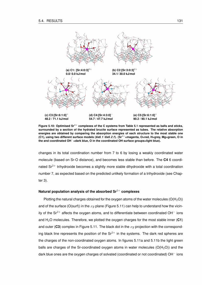
5.4. RESULTS 131
(a) C1: [Sr:4:0:3]2+
0.0/ 0.0 kJ/mol(b) C2:[Sr:3:0:3]2+
34.1/ 30.0 kJ/mol
(c) C3:[Sr:6:1:0]+
48.2 / 71.1 kJ/mol(d) C4:[Sr:4:3:0]−
54.7 / 47.7 kJ/mol(e) C5:[Sr:6:1:0]+
90.2 / 90.1 kJ/mol
Figure 5.10: Optimised Sr2+ complexes of the C systems from Table 5.1 represented as balls and sticks,surrounded by a section of the hydrated brucite surface represented as tubes. The relative absorptionenergies are obtained by comparing the absorption energies of each structure to the most stable one(C1), using two different surface models (6x6 1 /6x6 2 f ). (Sr2+=magenta, O=red, H=grey, Mg=green, O inthe and coordinated OH−=dark blue, O in the coordinated OH surface groups=light blue).
changes in its total coordination number from 7 to 6 by losing a weakly coordinated water
molecule (based on Sr-O distance), and becomes less stable than before. The C4 6 coordi-
nated Sr2+ trihydroxide becomes a slightly more stable dihydroxide with a total coordination
number 7, as expected based on the predicted unlikely formation of a trihydroxide (see Chap-
ter 3).
Natural population analysis of the absorbed Sr2+ complexes
Plotting the natural charges obtained for the oxygen atoms of the water molecules (O(H2O))
and of the surface (O(surf)) in the xy plane (Figure 5.11) can help to understand how the vicin-
ity of the Sr2+ affects the oxygen atoms, and to differentiate between coordinated OH− ions
and H2O molecules. Therefore, we plotted the oxygen charges for the most stable inner (C1)
and outer (C3) complex in Figure 5.11. The black dot in the xy projection with the correspond-
ing black line represents the position of the Sr2+ in the systems. The dark red spheres are
the charges of the non-coordinated oxygen atoms. In figures 5.11a and 5.11b the light green
balls are charges of the Sr-coordinated oxygen atoms in water molecules (O(H2O)) and the
dark blue ones are the oxygen charges of solvated (coordinated or not coordinated) OH− ions
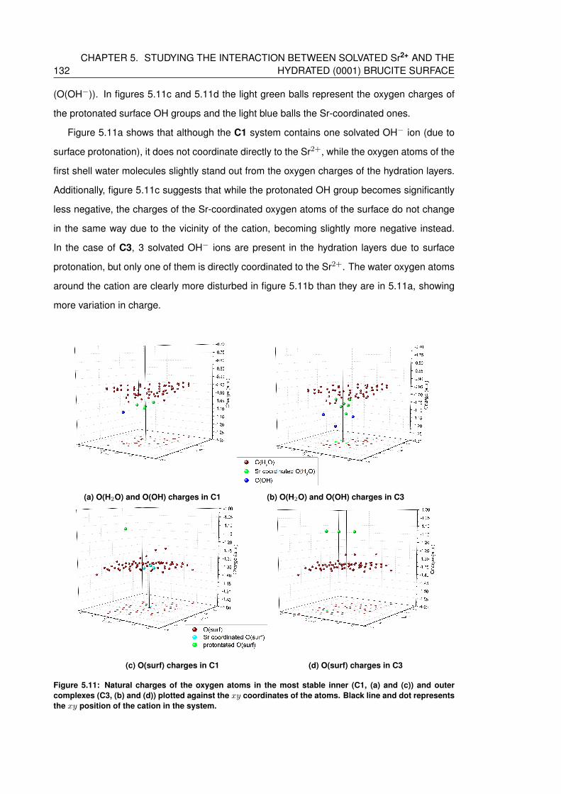
132CHAPTER 5. STUDYING THE INTERACTION BETWEEN SOLVATED Sr2+ AND THE
HYDRATED (0001) BRUCITE SURFACE
(O(OH−)). In figures 5.11c and 5.11d the light green balls represent the oxygen charges of
the protonated surface OH groups and the light blue balls the Sr-coordinated ones.
Figure 5.11a shows that although the C1 system contains one solvated OH− ion (due to
surface protonation), it does not coordinate directly to the Sr2+, while the oxygen atoms of the
first shell water molecules slightly stand out from the oxygen charges of the hydration layers.
Additionally, figure 5.11c suggests that while the protonated OH group becomes significantly
less negative, the charges of the Sr-coordinated oxygen atoms of the surface do not change
in the same way due to the vicinity of the cation, becoming slightly more negative instead.
In the case of C3, 3 solvated OH− ions are present in the hydration layers due to surface
protonation, but only one of them is directly coordinated to the Sr2+. The water oxygen atoms
around the cation are clearly more disturbed in figure 5.11b than they are in 5.11a, showing
more variation in charge.
(a) O(H2O) and O(OH) charges in C1 (b) O(H2O) and O(OH) charges in C3
(c) O(surf) charges in C1 (d) O(surf) charges in C3
Figure 5.11: Natural charges of the oxygen atoms in the most stable inner (C1, (a) and (c)) and outercomplexes (C3, (b) and (d)) plotted against the xy coordinates of the atoms. Black line and dot representsthe xy position of the cation in the system.

5.4. RESULTS 133
Collecting data from the natural population analysis of every structure in Table 5.2, shows
that the direct coordination of the Sr2+ lowers the average charge of the surface oxygen atoms
(from around -1.318 to -1.325). Moreover, every atom coordinated to the cation has a more
negative charge than the calculated average for that group of atoms.vi The standard deviation
of the oxygen atoms in the hydration layers (SD(hydr)) is smaller for the surface coordinated
complexes (∼0.036), as fewer O atoms are affected by the Sr2+, while it is higher (∼0.05)
for systems in which the ion is situated between the water layers. Differences in the cation
charges indicate that there is a relation between the Sr charge and the total number of coordi-
nated OH− ions (solvated): the Sr ion becomes less and less positive (C2, C1: 1.780, 1.777>
C5, C3: 1.764, 1.760 > C4: 1.734) as more OH− ions are in its first solvation shell (hydrates
> monohydroxides > trihydroxide). This observation indirectly suggests that the interactions
between the coordinated surface OH groups and the Sr, or the solvated OH− ions and the
cation, are qualitatively different, as they do not have the same effect on the Sr charge.
Table 5.2: Natural charges of the oxygen atoms for each Sr-coordinated OH surface group (O(surf)), H2Omolecule (O(H2O)) and solvated OH− ion (O(OH)), and the natural charge of the Sr atom, for the optimisedstructures in Figure 5.10 and Table 5.1. The average charge together with the corresponding standarddeviation was calculated for the surface oxygen atoms (AVE(surf) and SD(surf)) and the oxygen atoms inthe hydration layers (AVE(hydr) and SD(hydr)).
C1 C2 C3 C4 C5atom charge atom charge atom charge atom charge atom charge
O(surf) -1.352 O(surf) -1.351 O(OH) -1.197 O(OH) -1.184 O(OH) -1.245O(surf) -1.351 O(surf) -1.369 O(H2O) -1.114 O(OH) -1.198 O(H2O) -1.053O(surf) -1.345 O(surf) -1.355 O(H2O) -1.033 O(OH) -1.153 O(H2O) -1.062O(H2O) -1.086 O(H2O) -1.083 O(H2O) -1.081 O(H2O) -1.072 O(H2O) -1.032O(H2O) -1.070 O(H2O) -1.058 O(H2O) -1.063 O(H2O) -1.057 O(H2O) -1.090O(H2O) -1.085 O(H2O) -1.108 O(H2O) -1.027 O(H2O) -1.064 O(H2O) -1.063O(H2O) -1.056 - - O(H2O) -1.059 O(H2O) -1.075 O(H2O) -1.032
AV(surf) -1.325 AV(surf) -1.325 AV(surf) -1.319 AV(surf) -1.316 AV(surf) -1.318SD(surf) (0.037) SD(surf) (0.038) SD(surf) (0.051) SD(surf) (0.056) SD(surf) (0.046)AV(hydr) -1.013 AV(hydr) -1.013 AV(hydr) -1.028 AV(hydr) -1.030 AV(hydr) -1.024SD(hydr) (0.036) SD(hydr) (0.037) SD(hydr) (0.053) SD(hydr) (0.057) SD(hydr) (0.052)
Sr 1.777 Sr 1.780 Sr 1.760 Sr 1.734 Sr 1.764
The electron density difference plots of the C1 and C3 structures in Figure 5.12 show
that every ligand which is directly coordinated to the Sr2+ (even the surface OH groups) are
affected, most likely polarised, by the positive cation, which is presumably the reason for the
generally more negative oxygen charges calculated for the coordinated ligands in Table 5.2.
viThe average charges (AVE(surf) and AVE(hydr)) are calculated by considering only the charges of the unfixedoxygen atoms, as the boundary atoms may be affected by the surrounding point charges and by the fact that theircoordinates are frozen. AVE(hydr) contains the charge of every oxygen atom in the relaxed part of the hydrationlayer, even the O atoms of the solvated OH− ions.
134CHAPTER 5. STUDYING THE INTERACTION BETWEEN SOLVATED Sr2+ AND THE
HYDRATED (0001) BRUCITE SURFACE
The size of the red and blue regions in Figure 5.12 suggests that the effect of the Sr2+ is
relatively local, and does not go further than two coordination shells. Moreover, by comparing
the electron density difference plots of C1 and C3 with figure 4.17 in section 4.5.2, we can
conclude that in the presence of two hydration layers, the surface atoms are much less affected
by the cation than in the case of a Sr2+ hydrate with only three water molecules in its first
solvation shell.
(a) C1 (b) C3
Figure 5.12: Electron density distribution of the C1 (a) and C3 complexes (b). The isosurface value is0.0025 a.u.. The red regions indicate electron depletion, while the blue regions electron accumulation.The point charges are not shown. (Mg=pink, O=ochre, H=white, Sr=yellow)
5.4.2 Adsorption of Sr2+ hydroxides on a hydrated brucite surface
To observe the effect of differently charged environments on the adsorption, we replaced
one or two water molecules with OH− ions (in addition to the Sr2+ ion and the already existing
hydroxide ions due to the surface protonation). The results summarised in Table 5.3 (C OH2)
are obtained similarly to the those presented in the previous section, i.e. two structures were
optimised based on the 6x6 1 hydration model at different Sr-surface distances (C OH2 3
and C OH2 4) and the others were initiated from the deprotonation of C1 and C3. Systems
containing only one OH− ion in Table 5.4 are made by the protonation/deprotontation of the
previously optimised C OH2 and C structures and therefore discussed at last.
Considering the relative energies of the C OH2 structures in Table 5.3, we find that the
energy range of these values is close to those of the C systems in Table 5.1. Another similarity
is, that the two most stable structures (C OH2 1 and C OH2 2, see Figure 5.13) are effectively
Sr2+ hydrates directly coordinated to the surface; the introduced OH− ions are located in
the second coordination shell of the ion. The small energy difference between these two
complexes (21.2 kJ/mol) is most likely the consequence of changing one Sr-O(surf) to a Sr-
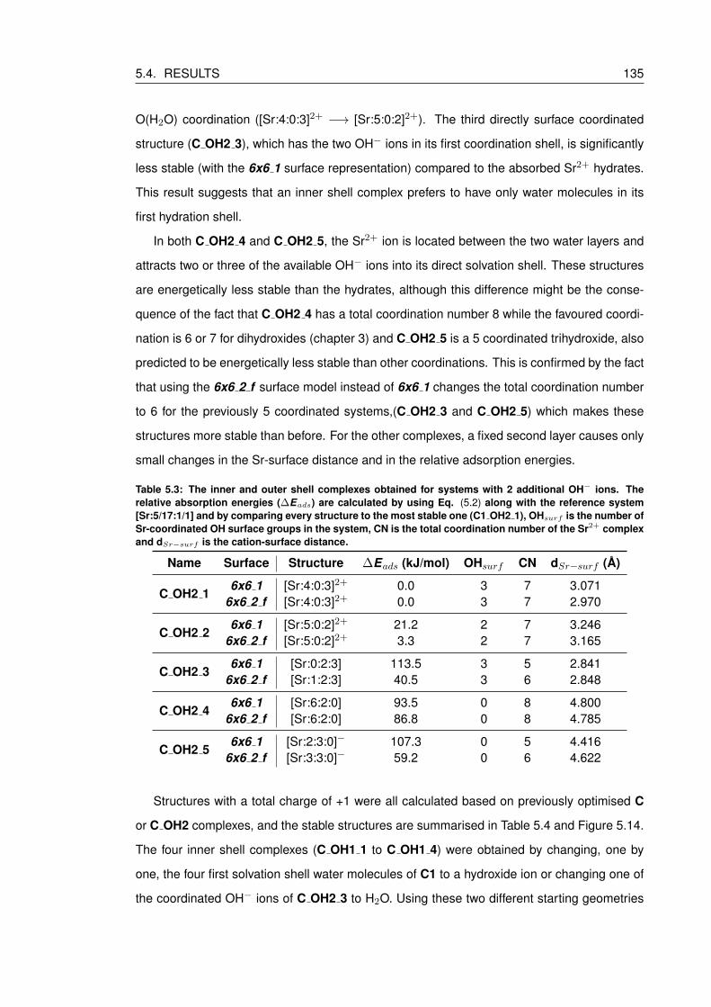
5.4. RESULTS 135
O(H2O) coordination ([Sr:4:0:3]2+ −→ [Sr:5:0:2]2+). The third directly surface coordinated
structure (C OH2 3), which has the two OH− ions in its first coordination shell, is significantly
less stable (with the 6x6 1 surface representation) compared to the absorbed Sr2+ hydrates.
This result suggests that an inner shell complex prefers to have only water molecules in its
first hydration shell.
In both C OH2 4 and C OH2 5, the Sr2+ ion is located between the two water layers and
attracts two or three of the available OH− ions into its direct solvation shell. These structures
are energetically less stable than the hydrates, although this difference might be the conse-
quence of the fact that C OH2 4 has a total coordination number 8 while the favoured coordi-
nation is 6 or 7 for dihydroxides (chapter 3) and C OH2 5 is a 5 coordinated trihydroxide, also
predicted to be energetically less stable than other coordinations. This is confirmed by the fact
that using the 6x6 2 f surface model instead of 6x6 1 changes the total coordination number
to 6 for the previously 5 coordinated systems,(C OH2 3 and C OH2 5) which makes these
structures more stable than before. For the other complexes, a fixed second layer causes only
small changes in the Sr-surface distance and in the relative adsorption energies.
Table 5.3: The inner and outer shell complexes obtained for systems with 2 additional OH− ions. Therelative absorption energies (∆Eads) are calculated by using Eq. (5.2) along with the reference system[Sr:5/17:1/1] and by comparing every structure to the most stable one (C1 OH2 1), OHsurf is the number ofSr-coordinated OH surface groups in the system, CN is the total coordination number of the Sr2+ complexand dSr−surf is the cation-surface distance.
Name Surface Structure ∆Eads (kJ/mol) OHsurf CN dSr−surf (A)
C OH2 16x6 1 [Sr:4:0:3]2+ 0.0 3 7 3.071
6x6 2 f [Sr:4:0:3]2+ 0.0 3 7 2.970
C OH2 26x6 1 [Sr:5:0:2]2+ 21.2 2 7 3.246
6x6 2 f [Sr:5:0:2]2+ 3.3 2 7 3.165
C OH2 36x6 1 [Sr:0:2:3] 113.5 3 5 2.841
6x6 2 f [Sr:1:2:3] 40.5 3 6 2.848
C OH2 46x6 1 [Sr:6:2:0] 93.5 0 8 4.800
6x6 2 f [Sr:6:2:0] 86.8 0 8 4.785
C OH2 56x6 1 [Sr:2:3:0]− 107.3 0 5 4.416
6x6 2 f [Sr:3:3:0]− 59.2 0 6 4.622
Structures with a total charge of +1 were all calculated based on previously optimised C
or C OH2 complexes, and the stable structures are summarised in Table 5.4 and Figure 5.14.
The four inner shell complexes (C OH1 1 to C OH1 4) were obtained by changing, one by
one, the four first solvation shell water molecules of C1 to a hydroxide ion or changing one of
the coordinated OH− ions of C OH2 3 to H2O. Using these two different starting geometries
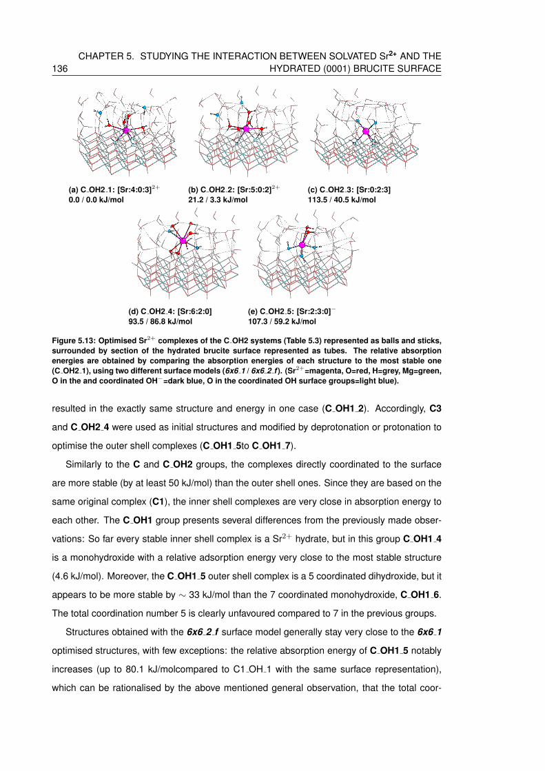
136CHAPTER 5. STUDYING THE INTERACTION BETWEEN SOLVATED Sr2+ AND THE
HYDRATED (0001) BRUCITE SURFACE
(a) C OH2 1: [Sr:4:0:3]2+
0.0 / 0.0 kJ/mol(b) C OH2 2: [Sr:5:0:2]2+
21.2 / 3.3 kJ/mol(c) C OH2 3: [Sr:0:2:3]113.5 / 40.5 kJ/mol
(d) C OH2 4: [Sr:6:2:0]93.5 / 86.8 kJ/mol
(e) C OH2 5: [Sr:2:3:0]−
107.3 / 59.2 kJ/mol
Figure 5.13: Optimised Sr2+ complexes of the C OH2 systems (Table 5.3) represented as balls and sticks,surrounded by section of the hydrated brucite surface represented as tubes. The relative absorptionenergies are obtained by comparing the absorption energies of each structure to the most stable one(C OH2 1), using two different surface models (6x6 1 / 6x6 2 f ). (Sr2+=magenta, O=red, H=grey, Mg=green,O in the and coordinated OH−=dark blue, O in the coordinated OH surface groups=light blue).
resulted in the exactly same structure and energy in one case (C OH1 2). Accordingly, C3
and C OH2 4 were used as initial structures and modified by deprotonation or protonation to
optimise the outer shell complexes (C OH1 5to C OH1 7).
Similarly to the C and C OH2 groups, the complexes directly coordinated to the surface
are more stable (by at least 50 kJ/mol) than the outer shell ones. Since they are based on the
same original complex (C1), the inner shell complexes are very close in absorption energy to
each other. The C OH1 group presents several differences from the previously made obser-
vations: So far every stable inner shell complex is a Sr2+ hydrate, but in this group C OH1 4
is a monohydroxide with a relative adsorption energy very close to the most stable structure
(4.6 kJ/mol). Moreover, the C OH1 5 outer shell complex is a 5 coordinated dihydroxide, but it
appears to be more stable by ∼ 33 kJ/mol than the 7 coordinated monohydroxide, C OH1 6.
The total coordination number 5 is clearly unfavoured compared to 7 in the previous groups.
Structures obtained with the 6x6 2 f surface model generally stay very close to the 6x6 1
optimised structures, with few exceptions: the relative absorption energy of C OH1 5 notably
increases (up to 80.1 kJ/molcompared to C1 OH 1 with the same surface representation),
which can be rationalised by the above mentioned general observation, that the total coor-
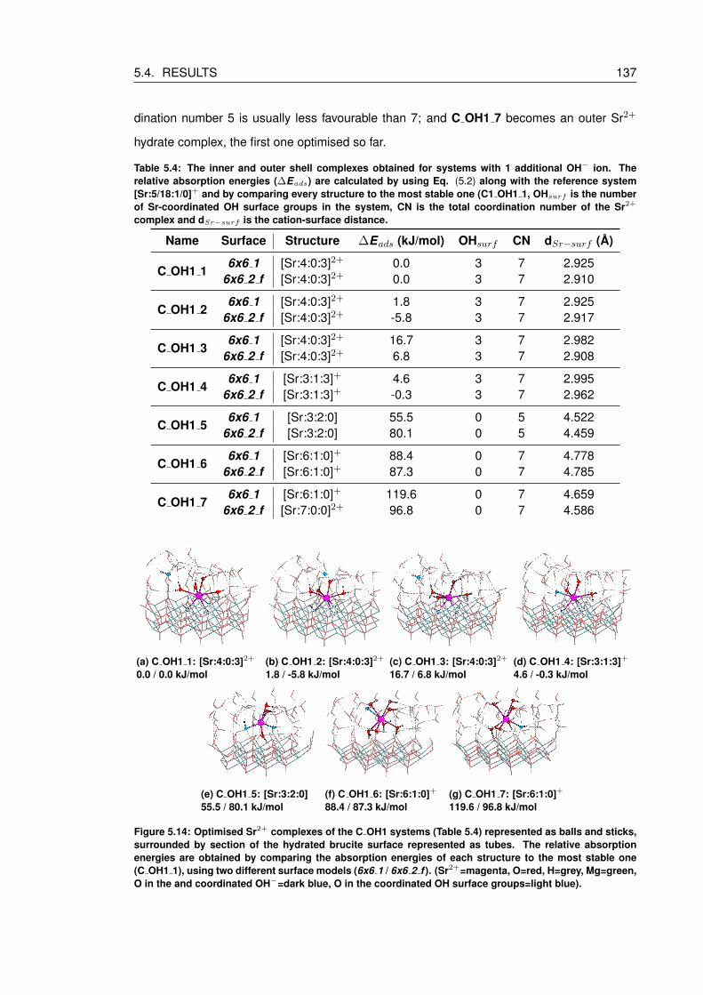
5.4. RESULTS 137
dination number 5 is usually less favourable than 7; and C OH1 7 becomes an outer Sr2+
hydrate complex, the first one optimised so far.
Table 5.4: The inner and outer shell complexes obtained for systems with 1 additional OH− ion. Therelative absorption energies (∆Eads) are calculated by using Eq. (5.2) along with the reference system[Sr:5/18:1/0]+ and by comparing every structure to the most stable one (C1 OH1 1, OHsurf is the numberof Sr-coordinated OH surface groups in the system, CN is the total coordination number of the Sr2+
complex and dSr−surf is the cation-surface distance.
Name Surface Structure ∆Eads (kJ/mol) OHsurf CN dSr−surf (A)
C OH1 16x6 1 [Sr:4:0:3]2+ 0.0 3 7 2.925
6x6 2 f [Sr:4:0:3]2+ 0.0 3 7 2.910
C OH1 26x6 1 [Sr:4:0:3]2+ 1.8 3 7 2.925
6x6 2 f [Sr:4:0:3]2+ -5.8 3 7 2.917
C OH1 36x6 1 [Sr:4:0:3]2+ 16.7 3 7 2.982
6x6 2 f [Sr:4:0:3]2+ 6.8 3 7 2.908
C OH1 46x6 1 [Sr:3:1:3]+ 4.6 3 7 2.995
6x6 2 f [Sr:3:1:3]+ -0.3 3 7 2.962
C OH1 56x6 1 [Sr:3:2:0] 55.5 0 5 4.522
6x6 2 f [Sr:3:2:0] 80.1 0 5 4.459
C OH1 66x6 1 [Sr:6:1:0]+ 88.4 0 7 4.778
6x6 2 f [Sr:6:1:0]+ 87.3 0 7 4.785
C OH1 76x6 1 [Sr:6:1:0]+ 119.6 0 7 4.659
6x6 2 f [Sr:7:0:0]2+ 96.8 0 7 4.586
(a) C OH1 1: [Sr:4:0:3]2+
0.0 / 0.0 kJ/mol(b) C OH1 2: [Sr:4:0:3]2+
1.8 / -5.8 kJ/mol(c) C OH1 3: [Sr:4:0:3]2+
16.7 / 6.8 kJ/mol(d) C OH1 4: [Sr:3:1:3]+
4.6 / -0.3 kJ/mol
(e) C OH1 5: [Sr:3:2:0]55.5 / 80.1 kJ/mol
(f) C OH1 6: [Sr:6:1:0]+
88.4 / 87.3 kJ/mol(g) C OH1 7: [Sr:6:1:0]+
119.6 / 96.8 kJ/mol
Figure 5.14: Optimised Sr2+ complexes of the C OH1 systems (Table 5.4) represented as balls and sticks,surrounded by section of the hydrated brucite surface represented as tubes. The relative absorptionenergies are obtained by comparing the absorption energies of each structure to the most stable one(C OH1 1), using two different surface models (6x6 1 / 6x6 2 f ). (Sr2+=magenta, O=red, H=grey, Mg=green,O in the and coordinated OH−=dark blue, O in the coordinated OH surface groups=light blue).

138CHAPTER 5. STUDYING THE INTERACTION BETWEEN SOLVATED Sr2+ AND THE
HYDRATED (0001) BRUCITE SURFACE
5.4.3 The relative stability of Sr2+ complexes on a hydrated brucite surface
In this section, we investigate the effect of the following factors on the adsorption energies:
the Sr-surface distance, the total coordination number, the number of Sr-coordinated solvated
OH− ions and the total number of OH− ions introduced in the system. In section 5.4.3.1 we
concentrate on the first three properties, while in section 5.4.3.2 we attempt to draw conclu-
sions regarding the number of OH− ions in the system. But first, we exclude the possibility
that the slight changes in the xy position of the Sr2+ during the optimisation process could
be related to the energy differences; a concern raised in section 4.5.2 for the absorption of
a single Sr2+ hydrate. By plotting the Sr x and y coordinates of each structure in a 3D plot
(Figure 5.15), we show that the differences in the final cation positions are very small and
that there is no direct relation between the obtained absorption energies and the Sr’s x and y
coordinates.
(a) (b)
Figure 5.15: (a) The xy projection of the Sr positions within the QM cluster, (b) the absorption energiesof every system from Table 5.1, 5.4 and 5.3 vs. the x and y Sr coordinates within the QM cluster. (Theboundary atoms of the QM cluster are projected on the xy plane as black dots, while the position of the Sratoms every adsorbed complexes are shown with white-grey-black balls.)
5.4.3.1 Interaction energies in different coordination regimes
Kerridge and Kaltsoyannis predicted three distinctive coordination regimes for Sr2+ hydrate
adsorption based on 38 possible complexes,[246] and a very similar conclusion is suggested
by plotting the relative adsorption energies of the optimised systems of section 5.4.1 and 5.4.2
as a function of dSr−surf , shown in Figure 5.16.
To study the possible relations between relative adsorption energies and the Sr-surface
distance in more detail, we chose one or two of the optimised surface coordinated com-
plexes of each group (for systems with 0,1 or 2 solvated OH− ions, the C1, C OH1 4, and
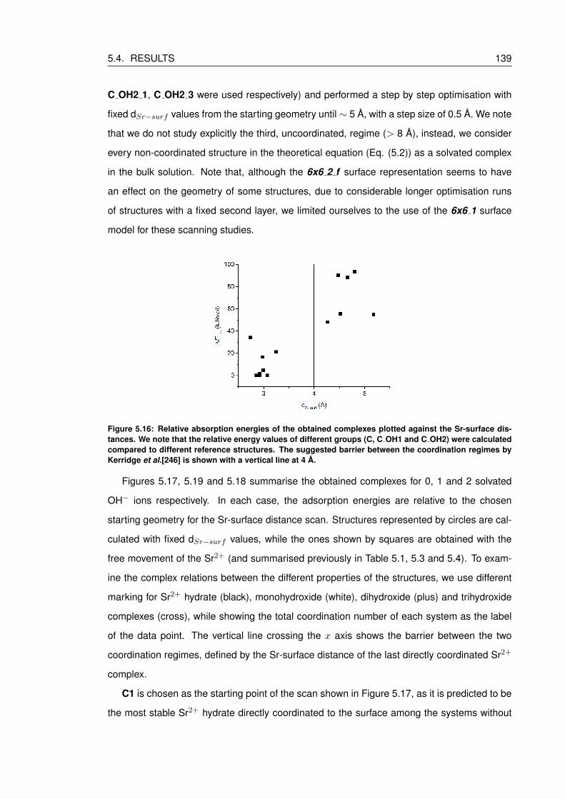
5.4. RESULTS 139
C OH2 1, C OH2 3 were used respectively) and performed a step by step optimisation with
fixed dSr−surf values from the starting geometry until∼ 5 A, with a step size of 0.5 A. We note
that we do not study explicitly the third, uncoordinated, regime (> 8 A), instead, we consider
every non-coordinated structure in the theoretical equation (Eq. (5.2)) as a solvated complex
in the bulk solution. Note that, although the 6x6 2 f surface representation seems to have
an effect on the geometry of some structures, due to considerable longer optimisation runs
of structures with a fixed second layer, we limited ourselves to the use of the 6x6 1 surface
model for these scanning studies.
Figure 5.16: Relative absorption energies of the obtained complexes plotted against the Sr-surface dis-tances. We note that the relative energy values of different groups (C, C OH1 and C OH2) were calculatedcompared to different reference structures. The suggested barrier between the coordination regimes byKerridge et al.[246] is shown with a vertical line at 4 A.
Figures 5.17, 5.19 and 5.18 summarise the obtained complexes for 0, 1 and 2 solvated
OH− ions respectively. In each case, the adsorption energies are relative to the chosen
starting geometry for the Sr-surface distance scan. Structures represented by circles are cal-
culated with fixed dSr−surf values, while the ones shown by squares are obtained with the
free movement of the Sr2+ (and summarised previously in Table 5.1, 5.3 and 5.4). To exam-
ine the complex relations between the different properties of the structures, we use different
marking for Sr2+ hydrate (black), monohydroxide (white), dihydroxide (plus) and trihydroxide
complexes (cross), while showing the total coordination number of each system as the label
of the data point. The vertical line crossing the x axis shows the barrier between the two
coordination regimes, defined by the Sr-surface distance of the last directly coordinated Sr2+
complex.
C1 is chosen as the starting point of the scan shown in Figure 5.17, as it is predicted to be
the most stable Sr2+ hydrate directly coordinated to the surface among the systems without
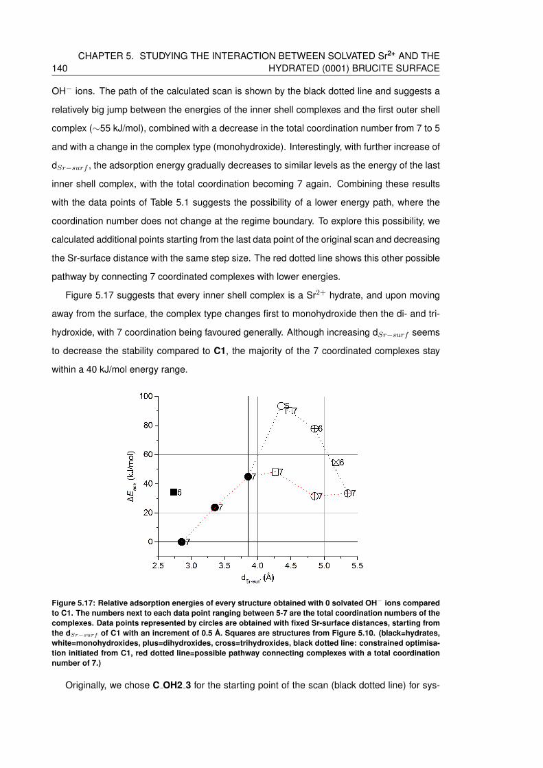
140CHAPTER 5. STUDYING THE INTERACTION BETWEEN SOLVATED Sr2+ AND THE
HYDRATED (0001) BRUCITE SURFACE
OH− ions. The path of the calculated scan is shown by the black dotted line and suggests a
relatively big jump between the energies of the inner shell complexes and the first outer shell
complex (∼55 kJ/mol), combined with a decrease in the total coordination number from 7 to 5
and with a change in the complex type (monohydroxide). Interestingly, with further increase of
dSr−surf , the adsorption energy gradually decreases to similar levels as the energy of the last
inner shell complex, with the total coordination becoming 7 again. Combining these results
with the data points of Table 5.1 suggests the possibility of a lower energy path, where the
coordination number does not change at the regime boundary. To explore this possibility, we
calculated additional points starting from the last data point of the original scan and decreasing
the Sr-surface distance with the same step size. The red dotted line shows this other possible
pathway by connecting 7 coordinated complexes with lower energies.
Figure 5.17 suggests that every inner shell complex is a Sr2+ hydrate, and upon moving
away from the surface, the complex type changes first to monohydroxide then the di- and tri-
hydroxide, with 7 coordination being favoured generally. Although increasing dSr−surf seems
to decrease the stability compared to C1, the majority of the 7 coordinated complexes stay
within a 40 kJ/mol energy range.
Figure 5.17: Relative adsorption energies of every structure obtained with 0 solvated OH− ions comparedto C1. The numbers next to each data point ranging between 5-7 are the total coordination numbers of thecomplexes. Data points represented by circles are obtained with fixed Sr-surface distances, starting fromthe dSr−surf of C1 with an increment of 0.5 A. Squares are structures from Figure 5.10. (black=hydrates,white=monohydroxides, plus=dihydroxides, cross=trihydroxides, black dotted line: constrained optimisa-tion initiated from C1, red dotted line=possible pathway connecting complexes with a total coordinationnumber of 7.)
Originally, we chose C OH2 3 for the starting point of the scan (black dotted line) for sys-
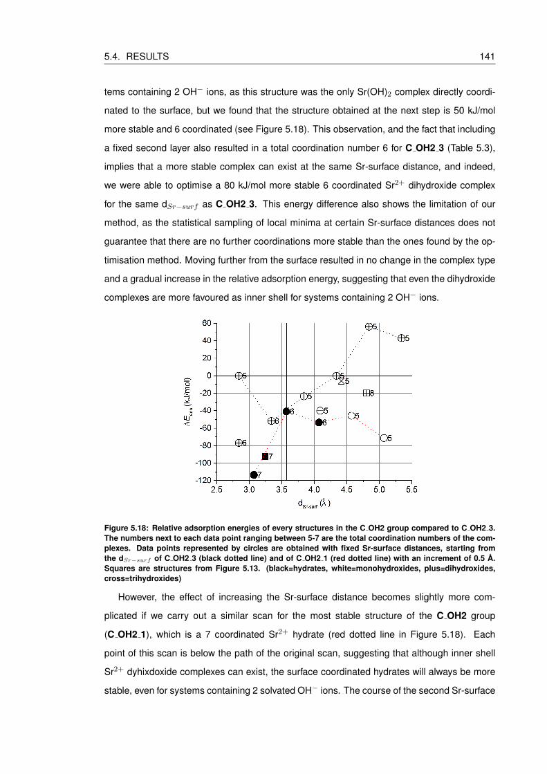
5.4. RESULTS 141
tems containing 2 OH− ions, as this structure was the only Sr(OH)2 complex directly coordi-
nated to the surface, but we found that the structure obtained at the next step is 50 kJ/mol
more stable and 6 coordinated (see Figure 5.18). This observation, and the fact that including
a fixed second layer also resulted in a total coordination number 6 for C OH2 3 (Table 5.3),
implies that a more stable complex can exist at the same Sr-surface distance, and indeed,
we were able to optimise a 80 kJ/mol more stable 6 coordinated Sr2+ dihydroxide complex
for the same dSr−surf as C OH2 3. This energy difference also shows the limitation of our
method, as the statistical sampling of local minima at certain Sr-surface distances does not
guarantee that there are no further coordinations more stable than the ones found by the op-
timisation method. Moving further from the surface resulted in no change in the complex type
and a gradual increase in the relative adsorption energy, suggesting that even the dihydroxide
complexes are more favoured as inner shell for systems containing 2 OH− ions.
Figure 5.18: Relative adsorption energies of every structures in the C OH2 group compared to C OH2 3.The numbers next to each data point ranging between 5-7 are the total coordination numbers of the com-plexes. Data points represented by circles are obtained with fixed Sr-surface distances, starting fromthe dSr−surf of C OH2 3 (black dotted line) and of C OH2 1 (red dotted line) with an increment of 0.5 A.Squares are structures from Figure 5.13. (black=hydrates, white=monohydroxides, plus=dihydroxides,cross=trihydroxides)
However, the effect of increasing the Sr-surface distance becomes slightly more com-
plicated if we carry out a similar scan for the most stable structure of the C OH2 group
(C OH2 1), which is a 7 coordinated Sr2+ hydrate (red dotted line in Figure 5.18). Each
point of this scan is below the path of the original scan, suggesting that although inner shell
Sr2+ dyhixdoxide complexes can exist, the surface coordinated hydrates will always be more
stable, even for systems containing 2 solvated OH− ions. The course of the second Sr-surface
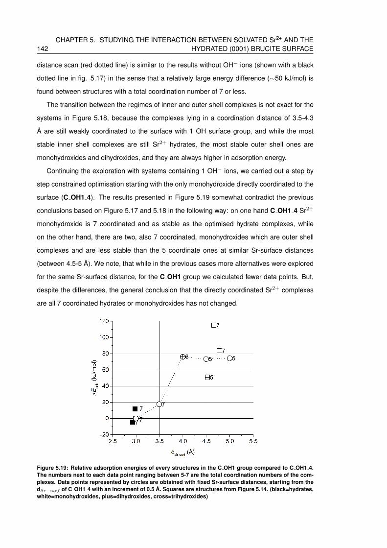
142CHAPTER 5. STUDYING THE INTERACTION BETWEEN SOLVATED Sr2+ AND THE
HYDRATED (0001) BRUCITE SURFACE
distance scan (red dotted line) is similar to the results without OH− ions (shown with a black
dotted line in fig. 5.17) in the sense that a relatively large energy difference (∼50 kJ/mol) is
found between structures with a total coordination number of 7 or less.
The transition between the regimes of inner and outer shell complexes is not exact for the
systems in Figure 5.18, because the complexes lying in a coordination distance of 3.5-4.3
A are still weakly coordinated to the surface with 1 OH surface group, and while the most
stable inner shell complexes are still Sr2+ hydrates, the most stable outer shell ones are
monohydroxides and dihydroxides, and they are always higher in adsorption energy.
Continuing the exploration with systems containing 1 OH− ions, we carried out a step by
step constrained optimisation starting with the only monohydroxide directly coordinated to the
surface (C OH1 4). The results presented in Figure 5.19 somewhat contradict the previous
conclusions based on Figure 5.17 and 5.18 in the following way: on one hand C OH1 4 Sr2+
monohydroxide is 7 coordinated and as stable as the optimised hydrate complexes, while
on the other hand, there are two, also 7 coordinated, monohydroxides which are outer shell
complexes and are less stable than the 5 coordinate ones at similar Sr-surface distances
(between 4.5-5 A). We note, that while in the previous cases more alternatives were explored
for the same Sr-surface distance, for the C OH1 group we calculated fewer data points. But,
despite the differences, the general conclusion that the directly coordinated Sr2+ complexes
are all 7 coordinated hydrates or monohydroxides has not changed.
Figure 5.19: Relative adsorption energies of every structures in the C OH1 group compared to C OH1 4.The numbers next to each data point ranging between 5-7 are the total coordination numbers of the com-plexes. Data points represented by circles are obtained with fixed Sr-surface distances, starting from thedSr−surf of C OH1 4 with an increment of 0.5 A. Squares are structures from Figure 5.14. (black=hydrates,white=monohydroxides, plus=dihydroxides, cross=trihydroxides)
5.4. RESULTS 143
5.4.3.2 The effect of solvated OH- ions
In this section, we attempt to understand the effect of the number of solvated hydroxide
ions on the absorption energies. Although we are aware that the systems with 0, 1 and 2
OH− ions carry a total charge of +2, +1 and 0 respectively, and applying the PEECM model
for differently charged systems can cause an artificial potential shift in the absolute absorption
energies, based on test calculations made for the adsorption of s block ions carrying +1 or +2
charge, we expect this error to be relatively small compared to the adsorption energies (see
section 4.5.1).
Figure 5.20 shows the absolute absorption energies of every system (both with relaxed
and fixed Sr2+ positions) as a function of the number of OH− ions in the system without
taking into account the effect of bulk solvent.vii The structures (both inner and outer shell
complexes), obtained for systems without additional OH− ions are all more stable by 250-340
kJ/mol compared with an empty hydrated brucite surface and a Sr2+ hydrate complex in the
bulk aqueous phase ([Sr:6/18:0/0]2+ from fig 3.6a). In contrast, the adsorbed complexes with
2 OH− ions introduced in the system all appear unfavourable by 40-210 kJ/mol compared with
the most stable hydroxide complex ([Sr:5/17:1/1] from table 3.8) in a solution containing the
same number of OH− ions. The absolute adsorption energies of the C OH1 structures lie
between the ones obtained for the C and C OH2 groups (from -115 to 5 kJ/mol) compared
with the most stable monohydroxide complex ([Sr:5/18:1/0]+). Overall, Figure 5.20 suggests
a high dependence on the total charge of the system and shows that in an environment where
solvated OH− ions are available next to the strontium, the formation of hydroxide species in
solution is more favourable than the adsorption of the Sr2+ on the hydrated (and protonated)
brucite surface.
However, the solvated reference structures used above are originally optimised with the
COSMO implicit solvent model, i.e. with a homogeneous background potential representing
the bulk aqueous phase. In this environment, the energy differences between the reference
structures using Eq. (3.2) in chapter 3 are the following: [Sr:6/18:0/0]2++2OH−: 0.0 kJ/mol >
[Sr:5/18:1/0]++OH−: -36.3 kJ/mol > [Sr:5/17:1/1]: -60.9 kJ/mol (see Figure 3.12a and Table
viiThe direct comparison of the energies is not straightforward, because, to keep the total charge equal in bothside of the theoretical equation (Eq. (5.2)), the reference systems are different for the three groups (C, C OH1,C OH2), i.e. for systems containing 0 OH− we chose a reference complex without solvated OH− etc. Therefore,using the same scale for the obtained energies of the three groups might be misleading. However, the referencecomplexes were energetically compared to each other with an other theoretical equation (Eq. (3.2)) in section 3,and after all, all energies are adsorption energies calculated to three different charge environment, which makesus to believe that they are reasonably comparable within the same scale.

144CHAPTER 5. STUDYING THE INTERACTION BETWEEN SOLVATED Sr2+ AND THE
HYDRATED (0001) BRUCITE SURFACE
Figure 5.20: Absolute absorption energies obtained by using Eq. 5.2 with the appropriate referencesystem for the C, C OH1 and C OH2 groups vs. the total number of solvated OH− ions in the system.(black=hydrates, white=monohydroxides, plus=dihydroxides, cross=trihydroxides)
3.13 in section 3.4.3). Using the same equation but without the COSMO method (gas phase)
and with def2-SVP basis sets dramatically changes the energies and enormously favours the
solvated 2OH− systems: 0.0 kJ/mol > -575.8 kJ/mol > -917.5 kJ/mol. As we cannot use the
COSMO and PEECM approaches at the same time, the adsorption energies shown in Figure
5.20 must be affected by this extreme difference in the relative energies of the reference
structures.
The importance of the basis set on the Sr2+ ion was explained previously in section 3.4.3.
However, due to the size of the whole PEECM system (∼ 396 atoms for 6x6 1 and 576 atoms
for 6x6 2 f ), applying higher quality basis sets for every atom type would be computationally
very expensive. Moreover, results in section 4.5.1 for the absorption of s block ions suggest
that larger basis set sizes on the surface atoms may have artificial side effects. Therefore, to
probe the possible effect of basis set size on the absorption energies, we carried out single
point calculations for every system in Table 5.1, 5.3 and 5.4 with def2-TZVP and def2-QZVP
basis set only on the Sr2+. The obtained adsorption energies are summarised in Table 5.5.
Applying the def2-TZVP on the cation decreases the absorption energies by c. 10 kJ/mol on
average for each group (C: 9.6 kJ/mol, C OH1: 8.2 kJ/mol and C OH2: 7.3 kJ/mol). Increasing
the basis set quality to quadruple-ζ decreases the absorption energies further by c. 0.1-
5.0 kJ/mol compared with the triple- and ∼ 7-14 kJ/mol compared with the double-ζ results.

5.4. RESULTS 145
Although the energy differences vary slightly between the different groups (and reference
systems), this deviation is relatively small and there is essentially a constant energy shift
between the double-ζ and higher basis sets.
Table 5.5: Dependence of the absolute adsorption energies (kJ/mol) on the basis set quality of the Sr2+
for systems from Table 5.1, 5.3 and 5.3 calculated with Eq. (5.2). (Standard deviations calculated for eachaverages are shown in brackets.)
systems def2-SVP ∆E(TZVP-SVP) def2-TZVP ∆E(QZVP-TZVP) def2-QZVP
C1 -338.1 -10.8 -348.9 -6.9 -355.8C2 -304.0 -12.7 -316.7 -4.6 -321.4C3 -289.9 -7.8 -297.7 -5.3 -303.0C4 -283.4 -7.2 -290.6 -2.6 -293.2C5 -247.9 -9.7 -257.6 -5.6 -263.2
average -9.6 (2.0) -5.0 (1.4)
C OH2 1 38.1 -5.9 32.2 -0.7 31.5C OH2 2 59.3 -8.9 50.3 -0.4 49.9C OH2 3 151.6 -8.2 143.4 1.8 145.2C OH2 4 131.6 -6.9 124.7 -0.1 124.6C OH2 5 145.4 -6.5 139.0 0.1 139.1
average -7.3 (1.1) 0.1 (0.9)
C OH1 1 -115.1 -7.3 -122.4 -3.9 -126.3C OH1 2 -113.3 -8.9 -122.2 -2.8 -125.0C OH1 3 -98.4 -9.9 -108.3 -2.5 -110.8C OH1 4 -110.5 -8.4 -118.9 -4.7 -123.7C OH1 5 -59.6 -7.0 -66.6 -1.8 -68.4C OH1 6 -26.7 -6.8 -33.5 -2.0 -35.5C OH1 7 4.5 -8.4 -3.9 -2.4 -6.2
average -8.1 (1.0) -2.9 (1.0)
We attempted to evaluate a COSMO correction term for the adsorbed complexes by using
a similar solvation scheme as Faheem et al.[298]. They proposed an approach called implicit
solvation model for solid surfaces (iSMS), in which they use a combination of periodic slab
calculations with plane wave DFT code in the absence of solvent and cluster models embed-
ded in the implicit continuum solvent to evaluate correct energies for the studied reactions; in
their case for the C-C bond cleavage of dehydrogenated ethylene glycol on Pt (111) in water.
To obtain constant correction terms for the three groups, first we evaluated the adsorption en-
ergies with the same theoretical equation (5.2) for every structure in each group, but with the
COSMO implicit solvent model on the W24 complexes (gas phase PEECM surface structures
vs COSMO solvated complexes). Then, we calculated COSMO single point energies for the
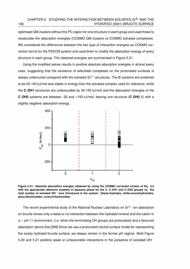
146CHAPTER 5. STUDYING THE INTERACTION BETWEEN SOLVATED Sr2+ AND THE
HYDRATED (0001) BRUCITE SURFACE
optimised QM clusters without the PC region for one structure in each group and used these to
recalculate the adsorption energies (COSMO QM clusters vs COSMO solvated complexes).
We considered the differences between the two type of interaction energies as COSMO cor-
rection terms for the PEECM system and used them to modify the absorption energy of every
structure in each group. The obtained energies are summarised in Figure 5.21.
Using the modified values results in positive absolute adsorption energies in almost every
case, suggesting that the existence of adsorbed complexes on the protonated surfaces is
always unfavoured compared with the solvated Sr2+ structures. The C systems are predicted
to be 50-140 kJ/mol less stable in energy than the solvated complex used for reference, while
the C OH1 structures are unfavourable by 30-150 kJ/mol and the adsorption energies of the
C OH2 systems are between -20 and +150 kJ/mol, leaving one structure (C OH2 1) with a
slightly negative adsorption energy.
Figure 5.21: Absolute absorption energies obtained by using the COSMO corrected version of Eq. 5.2with the appropriate reference systems in aqueous phase for the C, C OH1 and C OH2 groups vs. thetotal number of solvated OH− ions introduced in the system. (black=hydrates, white=monohydroxides,plus=dihydroxides, cross=trihydroxides)
The recent experimental study of the National Nuclear Laboratory on Sr2+ ion adsorption
on brucite shows only a weak or no interaction between the hydrated mineral and the cation in
a < pH 11 environment, (i.e. when the terminating OH groups are protonated) and a favoured
adsorption above that.[299] Since we use a protonated neutral surface model for representing
the empty hydrated brucite surface, we always remain in the former pH regime. Both Figure
5.20 and 5.21 predicts weak or unfavourable interactions in the presence of solvated OH−
5.5. CONCLUSIONS 147
ions, but the COSMO corrected results show a generally unfavoured interaction regardless
of the charge environment. Since the model used in Figure 5.21 considers the reference
systems in aqueous phase and contains a limited solvent correction for surface model too, we
assume that it represents a more realistic picture and therefore its results are closer to the
true values. However, by artificially combining two originally incompatible methods (PEECM
and COSMO), we may introduce unexpected errors during the ”tailoring” which cannot occur
when every component of the equations is in gas phase.
5.5 Conclusions
To study the interaction which is the main focus of this project, namely the adsorption be-
haviour of Sr2+ ions on brucite in the aqueous phase, the previously optimised PEECM model
was improved by introducing hydration layers above the surface and a theoretical equation
was used to evaluate adsorption energies. Overall, we found that the adosrption of Sr2+
hydrates and hydroxides is not favoured close to neutral pH conditions.
To model water layers above the surface cluster, the initial geometries of the explicit water
molecules and the positions of the point charge water equivalents are based on the molecu-
lar dynamic studies of Sakuma et al.[278] The final model contains 2 hydration layers in the
so-called C water coordination, with 72 explicit water molecules in the QM cluster above the
surface. During the optimisation, spontaneous surface protonation occurred between the first
layer water molecules and the up-facing OH groups of brucite, which resulted in two solvated
OH− ions in the hydration layers. The formation of positive surface species in neutral solu-
tions is expected on the basis of the experimental study of Pokrovosky and Schott[268] and
therefore we proceeded with that optimised model without further corrections.
The Sr2+ was introduced to the system by placing it at different distances from the sur-
face but always in the middle of the QM cluster. Systems containing 0, 1 and 2 additional
solvated OH− ions, were examined to study the effect of differently charged environments.
The structures of the Sr complexes obtained were analysed based on their total coordination
number, the Sr-surface distance and the number of directly coordinated OH− ions or OH sur-
face groups. The adsorption energies were calculated from an equation which compares the
energy of the adsorbed Sr2+ ions with the energy of the chosen W24 water cluster based
reference systems in gas phase and with an additional COSMO correction term.
Structures obtained in each of the three different groups (C, C OH1, C OH2) are all in a
∼100-120 kJ/mol energy range, which is reasonable considering the fact that they may vary
148CHAPTER 5. STUDYING THE INTERACTION BETWEEN SOLVATED Sr2+ AND THE
HYDRATED (0001) BRUCITE SURFACE
in their hydrogen bond network as well as in the Sr coordination, and test calculations show
that, for example, the energy gain by the formation of a single hydrogen bond is ∼14 kJ/mol
between two water molecules and ∼50 kJ/mol between an OH− ion and a water molecule.
After analysis of the optimised complexes in Figure 5.10, 5.13 and 5.14 and further studies
of the Sr-surface distance relations by constrained optimisations in Figure 5.17, 5.18 and
5.19, we can conclude that generally the inner shell complexes tend to be more stable than
the outer shell ones. In addition, the most stable directly surface coordinated structures are
usually Sr2+ hydrates with a total coordination number of 7. This result is consistent with
previous solvation studies, which predict the most stable coordination of a hydrated complex
to be between 6 or 8 (see chapter 3). Gradually moving away from the surface, the outer
shell complexes, with only a few exceptions, have a lower total coordination number as well
as more OH− ions coordinated to the cation than the inner shell ones.
Using a surface model 6x6 2 f to account for the effect of a second brucite layer on the
adsorption, in some cases affects the geometries and the absorption energies, but usually
only for the less stable complexes. The most stable ones and the general energetic order are
unaffected. This observation is supported by the electron density difference plots of structures
C1 and C3, where we see smaller contributions from the surface groups (Figure 5.12) than in
the case of adsorbed complexes on a bare brucite surface (Figure 4.12 and 4.17).
The natural charges in the C structures show a clear difference between the oxygen atoms
of the solvated OH− ions and the OH surface groups, as well as suggest a qualitative differ-
ence between Sr-O(surf) and Sr-O(OH) coordinations. The obtained oxygen charges (Table
5.2) together with the electron density difference plots (Figure 5.12) show the relatively local
effect of the cation and the polarisation of the directly coordinated O atoms.
Finally, we attempted to study the effect of differently charged aqueous environments on
the adsorption behaviour, by comparing the obtained adsorption energies of the C, C OH1
and C OH2 groups. In the gas phase, the Sr-brucite interaction is unfavoured in the presence
of additional OH− ions; while based on COSMO corrected energies, the adsorption of Sr
species on brucite is generally unfavoured in the aqueous phase, which is consistent with
recent experimental results in below pH 11 conditions. Based on these results, we conclude
that our PEECM-COSMO model of the (0001) surface successfully describes the interaction
of Sr complexes and hydrated (0001) surface in neutral conditions.
Chapter 6
Conclusions
In this chapter, we reflect back on our original computational goals and results, how well
they have been accomplished and what are the possible ways forward. We also draw a final
conclusion based on our findings for the proposed industry related question: what are the
possible interactions between Sr2+ and brucite surfaces?
6.1 Computational achievements
6.1.1 Studying the hydrolysis of Sr2+ in aqueous environment
The accurate modelling of solvated Sr2+ hydroxide complexes was an important first step
for creating a reference system for the ion’s behaviour in the liquid phase of the nuclear storage
ponds (see section 1.4.1). While Sr2+ hydrates were extensively studied before, the formation
hydroxide complexes in water has not been modelled so far. In our DFT based computational
study presented in chapter 3, we showed the importance of carrying out geometry optimisa-
tions with the use of an implicit solvent model and with a sufficiently large explicit solvation
shell in investigating the structure and energetics of Sr2+ hydroxide complexes.
We used the W24 water cluster (which has been employed for modelling the solvation shell
of organic molecules and ions before but not of single ions) as the first two solvation shell of
Sr, because on one hand, it contained enough number of water molecules to account for
maximum 8 Sr coordinated waters and 2 additional water molecules for each first shell ligand;
and on the other hand, it allowed us to establish proton transfer with a small energy barrier and
predict the generally less favoured hydroxide complexes (tri- and tetrahydroxide). However, we
note that treating systems containing negatively charged species is generally difficult in implicit
solvent models due to the more diffuse nature of negative charge, and therefore systems with
and overall negative charge are usually avoided.
Overall, with the use of a combined implicit and explicit solvent model containing both the
first and second hydration shells, we found that the mono- and dihydroxides are the thermody-
namically most stable Sr complexes in a high pH aqueous solution and that they coexist. The
obtained stable species play an important role in chapter 5, where they are used to calculate
the stability Sr2+ complexes adsorbed on the (0001) surface of brucite.
149

150 CHAPTER 6. CONCLUSIONS
Based on the successful prediction of the energetics of Sr2+ hydrolysis, we suggest that a
similar model could be applied to study the solvation of other relevant ions and complexes in
the nuclear waste industry, such as the much less investigated Cs+, or the carbonate complex
of strontium.
6.1.2 Creating a suitable surface representation of (0001) brucite surface
A significant part of this thesis is concerned with optimising a surface model for studying
the adsorption of Sr2+ on the hydrated (0001) brucite surface (chapter 4). To meet with the
specified requirements in section 1.4.2, we decided to employ a PEECM model, because it is
implemented in the same code we used for the solvation study, it describes isolated adsorption
sites and charged systems, does not require supercomputers to run and our main interest is
the local environment of the possible reactions and we were less concerned with the large-
scale surface properties.
Surface models, containing one or two layers in the QM cluster and iteratively defined nat-
ural charges in the PC region, were optimised and validated through several model adsorption
studies involving single ions and Sr complexes. To verify that the PEECM model is as capable
of describing adsorption on the brucite surface as well as other periodic DFT based methods,
we carried out further test investigations comparing the energies obtained with the two dif-
ferent methods, with great success. As opposed to other previously modelled surfaces with
PEECM, brucite (0001) is not purely ionic and has a layered structure with a large interfacial
distance. Our research showed that this method can be successfully extended to be applied
to the most stable surface of brucite, and hopefully it will be used for similar materials in the
future.
As the purpose of the completed test calculations were to prove that the PEECM model
gives realistic energetic orders for the adsorption of Sr and other alkaline metal ions, we did
not investigated the structural differences of individual structures in detail and did not ex-
plore the possibility to improve every test system further with introducing hydration or solvent
molecules. This could be the subject of an individual study in which the presented single ion
adsorption and substitution could be extended with similar solvation models as it was estab-
lished in chapter 5 and more in-depth structural analysis could be do to justify the experienced
differences between ions.
6.1. COMPUTATIONAL ACHIEVEMENTS 151
6.1.3 Studying the interactions between the solvated Sr2+ and hydrated (0001)
brucite surface
Perhaps the greatest challenge of this project was to combine the approaches applied in
chapter 3 and 4 to investigate the adsorption of Sr2+ hydrate and hydroxide complexes on
a hydrated (0001) surface. To allow this, we extended the established surface model with
layers of water above it. To the best of our knowledge, although other QM/MM methods have
been employed to model hydrated surfaces before, the PEECM has not yet been used for
such problems. We used the results of previous MD studies to introduce water molecules
both within the QM and PC region. Although we simplified our model by only using one of the
predicted stable water coordinations, the created model gave reasonable results compared
with experimental findings, e.g. it predicted the protonation of surface species. However, it is
possible that with the construction of an optimised water cluster based on more than one type
of the MD simulated water positions in the PC and QM region, the created hydrated surface
model would be even more realistic, at least more in agreement with the MD results.
We used a theoretical reaction to compare the energies of Sr complexes adsorbed to the
hydrated brucite surface and solvated in water, and calculated adsorption energies ion with or
without additional hydroxides available in the water layers. With the application of a COSMO
correction to account for long-range solvation effects, we came to the main conclusion that the
interaction between the Sr2+ cation and brucite (0001) is unfavoured in below pH 11 aqueous
environment. This results agreed with the recent experimental findings and made us believe
that the application of the PEECM model and the three step approach for investigating the
interactions between the Sr ion and the (0001) brucite surface presented in this thesis, can be
generalised and employed to other problems of nuclear relevance, such as uranyl ion transport
in common soil components or sorption mechanisms in zeolite type ion exchangers.
The whole project was carried out using different implementations of the TURBOMOLE
program, which makes the investigation relatively simple. Since this code does not require a
massively parallelised version and it can be run efficiently on a local computer server (see sec-
tion 2.7.4.1), the presented calculations are very cost efficient making the developed process
a viable alternative for studying surface mechanisms on similar surface.
6.1.4 Future Works
We propose several possible ways where this project could directly progress, such as
the solvation study of Cs+ or carbonated strontium with the combined explicit-implicit solvent
152 CHAPTER 6. CONCLUSIONS
model and the extended study of ionic adsorption and substitution on brucite (0001) involving
other industrially relevant alkaline earth ions and their detailed structural analysis. Subse-
quently, the description of the hydrated brucite surface could be improved by considering a
combination of the MD predicted water coordinations in the PC and QM region or, as an alter-
native hydrated surface model, the application of a droplet-like water cluster above the surface
without water equivalents in the PC region could be explored.
As the solvation/hydrolysis of Sr2+ and its behaviour at the water/brucite interface is a
dynamic phenomenon with average coordination properties, ab initio MD simulations would
be perfect to complement our study. A similar project is already on-going in the research
group of Dr Andy Kerridge at Lancaster University by Olivia Lynes who also uses the herein
optimised structures as templates for further investigation. However, based on this work and
the recent experimental results of NNL, the Sr/brucite interaction is insignificant in the sludge
when the brurcite surface is protonated,[299] and investigating the other surfaces of brucite or
even other minerals might be more useful.
6.2 Industrial relevance
As far as our model can predict, there are no favoured interactions, between the solvated
Sr2+ complexes and the hydrated (0001) brucite surface in < pH 11 conditions where the
solvated complexes are always be more favourable than the adsorbed ones. These findings
are backed with recent experimental results, which show no significant interaction between the
brucite and Sr2+ ion below pH 11 solutions.[299] Nonetheless, a significant strontium uptake
is detected in the settling tanks of the ion exchange process, i.e. some material which has a
bigger particle size interacts with the ion. Therefore the question remains, what happens to
the strontium in the ponds?
One possibility is that the majority of the Sr2+ ions are carbonated by dissolved carbon
dioxide and the formed Sr-carbonate complexes interact with the brucite surface similarly to
reported uranyl-carbonate complexes [12]. However, SrCO3 most likely precipitates from the
solution as a white powder, since it is practically insoluble in water (unless the solution is not
saturated with carbon dioxide). In case of precipitation, the usual particle size of the SrCO3 is
small (submicron), thus it is more likely to be filtered out in the sand bed filters than remain in
the settling tanks, where the uptake was measured.
The fact that some sorption capacity was measured for Sr2+ on brucite [14], could be due
to other, non-basal surfaces. In the case of similar minerals to brucite, it is sometimes reported

6.2. INDUSTRIAL RELEVANCE 153
that surface protonation/deprotonation, which create possible adsorption sites for future ionic
interactions, can occur only on lateral surfaces.[300, 301] However, since the (0001) basal
surface is by far the most stable and therefore the most common surface of brucite, even if the
Sr2+ ion favourably interacts with the edges, they are so much less common, that they cannot
possibly be solely responsible for the significant strontium uptake.
Overall, it is more likely that another material, which co-exists with the formed magnesium-
hydroxide in the solid phase, adsorbs the Sr2+ complexes. According to Gregson et al.[11],
there are other Mg based phases, such as hydrotalcite and Mg-hydroxycarbonate, together
with in-situ formed uranium oxide particles within the corroded Magnox sludge. Preliminary
experimental results predict possible interactions between uranium oxide and Sr2+, therefore
the industrially most useful continuation of this project would be to investigate those interac-
tions with computational methods.
Bibliography
1J. J. Hastings, D. Rhodes, A. S. Fellerman, D. Mckendrick, and C. Dixon, “New approaches
for sludge management in the nuclear industry”, Powder Technology 174, 18–24 (2007).
2S. Owens, M. Higgins-Bos, M. Bankhead, and J. Austin, “Using Chemical And Process
Modelling to Design, Understand and Improve an Effluent Treatment Plant”, NNL Science,
4–13 (2015).
3S. E. Jensen and E. Nonbøl, Description of the Magnox Type of Gas Cooled Reactor (MAG-
NOX), November (Risø National Laboratory, Roskilde, Denmark, 1999), pp. 1–83.
4P. Greenfield, “A Comparison of Magnox A 12 and ZA Alloys as Canning Materials for
Nuclear Reactors”, Journal of Nuclear Materials 11, 121–134 (1964).
5G. T. Higgins, “Secondary Recrystallisation in Magnox AL 80”, Journal of Nuclear Materials
8, 153–159 (1963).
6G. T. Higgins and B. W. Pickles, “Some observations of the pick-up of hydrogen in MAGNOX
ZR 55 and its relation to mechanical properties”, Journal of Nuclear Materials 8, 160–168
(1963).
7Photo Credit: Prof. B. Marsden, University of Manchester, NGRG, Oldbury visit part one,
Oldbury MAGNOX fuel element in graphite brick - http://www.nuclearbritain.com.
8Sellafield Ltd., Risk&Hazard Solution, http://www.sellafieldsites.com.
9M. E. Pick, “Magnox Graphite Core Decommissioning and Disposal Issues”, in Progress in
radioactive graphite waste management (Waste Technology Section , International Atomic
Energy Agency, Vienna International Centre, 2010), pp. 1–14.
10Nuclear Decommissioning Authority, Deparment of Energy & Climate Change, Radioactive
Wastes in the UK : A Summary of the 2013 Inventory, tech. rep. (2013), pp. 1–15.
11C. R. Gregson, D. T. Goddard, M. J. Sarsfield, and R. J. Taylor, “Combined electron mi-
croscopy and vibrational spectroscopy study of corroded Magnox sludge from a legacy
spent nuclear fuel storage pond”, Journal of Nuclear Materials 412, 145–156 (2011).
12Q. Cao, F. Huang, Z. Zhuang, and Z. Lin, “A study of the potential application of nano-
Mg(OH)2 in absorbing low concentrations of uranyl tricarbonate from water”, Nanoscale 4,
2423–2430 (2012).
13J. D. Farr, M. P. Neu, R. K. Schulze, and B. D. Honeyman, “Plutonium uptake by brucite and
hydroxylated periclase”, Journal of Alloys and Compounds 444-445, 533–539 (2007).
154
BIBLIOGRAPHY 155
14G. R. Bochkarev and G. I. Pushkareva, “Mineral Dressing - Strontium Removal from Aqeous
Media by Natural and Modified Sorbents”, Journal of Mining Science 45, 290–294 (2009).
15S. H. Wallace, S. Shaw, K. Morris, J. S. Small, A. J. Fuller, and I. T. Burke, “Effect of ground-
water pH and ionic strength on strontium sorption in aquifer sediments: Implications for 90Sr
mobility at contaminated nuclear sites”, Applied Geochemistry 27, 1482–1491 (2012).
16A. J. Francis, C. J. Dodge, and T. Ohnuki, “Microbial Transformations of Plutonium”, Journal
of Nuclear and Radiochemical Sciences 8, 121–126 (2007).
17H. Boukhalfa, G. A. Icopini, S. D. Reilly, and M. P. Neu, “Plutonium(IV) Reduction by the
Metal-Reducing Bacteria Geobacter metallireducens GS15 and Shewanella oneidensis
MR1.”, Applied and Environmental Microbiology 73, 5897–5903 (2007).
18K. Hirose and M. Aoyama, “Chemical speciation of plutonium in seawater”, Analytical and
Bioanalytical Chemistry 372, 418–420 (2002).
19W. Runde, S. D. Conradson, D. W. Efurd, N. Lu, C. E. VanPelt, and C. D. Tait, “Solubility
and sorption of redox-sensitive radionuclides (Np, Pu) in J-13 water from the Yucca Moun-
tain site: comparison between experiment and theory”, Applied Geochemistry 17, 837–853
(2002).
20G. Meinrath, “Uranium (VI) speciation by spectroscopy”, Journal of Radioanalytical and
Nuclear Chemistry 224, 119–126 (1997).
21D. Langmuir, “Uranium Solution - Mineral Equilibria at Low Temperatures with Applications
to Sedimentary Ore Deposits”, Geochimica et Cosmochimica Acta 42, 547–569 (1978).
22A. L. Nichols, D. L. Aldama, and M. Verpelli, “C-3.3. U-235 cumulative fission yields for se-
lected fission products”, in Handbook of nuclear data for safeguards: database extensions,
August (Nuclear Data Section , International Atomic Energy Agency, Wagramer Strasse 5,
A-1400 Vienna, Austria, 2008), pp. 105–106.
23M.-M. Be, V. Chiste, C. Dulieu, E. Browne, C. Baglin, V. Chechev, N. Kuzmenco, R. Helmer,
F. Kondev, D. MacMahon, and K. B. Lee, in Table of radionuclides - a=3 to 244, Vol. 3,
Monographie BIPM-5 (Bureau International des Poids et Mesures, Pavillon de Breteuil,
F-92310 Sevres, France, 2006).
24D. Di Tommaso and N. H. de Leeuw, “First principles simulations of the structural and
dynamical properties of hydrated metal ions Me2+ and solvated metal carbonates (Me =
Ca, Mg, and Sr)”, Crystal Growth and Design 10, 4292–4302 (2010).
25Some aspects of strontium radiobiology, Vol. Report No. 110 (NCRP, National Council on
Radiation Protection and Measurements, Bethesda, MD, 1991), p. 94.
156 BIBLIOGRAPHY
26United States Environmental Protection Agency, Radiation Protection - Radionuclide Ba-
sics, http://www.epa.gov.
27F. Cadini, E. Tosoni, and E. Zio, “Modeling the release and transport of 90Sr radionuclides
from a superficial nuclear storage facility”, Stochastic Environmental Research and Risk
Assessment 30, 693–712 (2016).
28Z. Maher, J. Storey, J. Rawcliffe, D. Goddard, L. O’Brien, and N. Bryan, Actinide Abatement
in SIXEP, tech. rep. (University of Manchester, 2012).
29J. E. Earp and D. R. Thompson, “Radio Active Waste Plants - Back to the Future - 8324”,
in Proceedings of the WM2008 Conference (2008).
30Ion Exchange Application in Wastewater Treatment, http://www.wastewatersystem.net.
31International Atomic Energy Agency, “Application of Ion Exchange Processes for the Treat-
ment of Radioactive Waste and Management of Spent Ion Exchangers”, Technical reports
series No.408 (2002).
32S. A. Fuente, C. A. Ferretti, N. F. Domancich, V. K. Dıez, C. R. Apesteguıa, J. I. Di Cosimo,
R. M. Ferullo, and N. J. Castellani, “Adsorption of 2-propanol on MgO surface: A combined
experimental and theoretical study”, Applied Surface Science 327, 268–276 (2015).
33J. R. B. Gomes and J. A.N. F. Gomes, “Adsorption of the formyl species on transition metal
surfaces”, Journal of Electroanalytical Chemistry 483, 180–187 (2000).
34X.-Y. Pang, C. Wang, Y.-H. Zhou, J.-M. Zhao, and G.-C. Wang, “DFT study of the structure
sensitivity for the adsorption of methyl, methoxy, and formate on Ni(111), Ni(100), and
Ni(110) surfaces”, Journal of Molecular Structure: THEOCHEM 948, 1–10 (2010).
35E. Veilly, J. Roques, M.-C. Jodin-Caumon, B. Humbert, R. Drot, and E. Simoni, “Uranyl
interaction with the hydrated (001) basal face of gibbsite: A combined theoretical and spec-
troscopic study”, Journal of Chemical Physics 129, 244704 (2008).
36K. W. Corum and S. E. Mason, “Establishing trends in ion adsorption on the aqueous
aluminium hydroxide nanoparticle Al30”, Molecular Simulation 41, 146–155 (2015).
37S. Chretien and H. Metiu, “Density functional study of the charge on Aun clusters (n=1-7)
supported on a partially reduced rutile TiO2(110): Are all clusters negatively charged?”,
Journal of Chemical Physics 126, 104701 (2007).
38H. Weber, T. Bredow, and B. Kirchner, “Adsorption Behavior of the 1,3-Dimethylimidazolium
Thiocyanate and Tetracyanoborate Ionic Liquids at Anatase (101) Surface”, Journal of
Physical Chemistry C 119, 15137 (2015).

BIBLIOGRAPHY 157
39S. K. Ramadugu and S. E. Mason, “DFT Study of Antimony (V) Oxyanion Adsorption on
α-Al2O3 (1102)”, Journal of Physical Chemistry C 119, 18149–18159 (2015).
40S. E. Mason, C. R. Iceman, K. S. Tanwar, T. P. Trainor, and A. M. Chaka, “Pb(II) Adsorption
on Isostructural Hydrated Alumina and Hematite (0001) Surfaces: A DFT Study”, Journal
of Physical Chemistry C 113, 2159–2170 (2009).
41S. Yang, C. Chen, Y. Chen, J. Li, D. Wang, X. Wang, and W. Hu, “Competitive Adsorption of
PbII , NiII , and SrII Ions on Graphene Oxides: A Combined Experimental and Theoretical
Study”, ChemPlusChem 80, 480–484 (2015).
42G. Garcıa, M. Atilhan, and S. Aparicio, “Adsorption of choline benzoate ionic liquid on
graphene, silicene, germanene and boron-nitride nanosheets: a DFT perspective”, Physcal
Chemistry Chemical Physics 17, 16315–16326 (2015).
43X. Tan, M. Fang, and X. Wang, “Sorption Speciation of Lanthanides/Actinides on Minerals
by TRLFS, EXAFS and DFT Studies: A Review”, Molecules 15, 8431–8468 (2010).
44J. A. Greathouse, R. J. O’Brien, G. Bemis, and R. T. Pabalan, “Molecular Dynamics Study
of Aqueous Uranyl Interactions with Quartz (010)”, The Journal of Physical Chemistry B
106, 1646–1655 (2002).
45S. Lectez, J. Roques, M. Salanne, and E. Simoni, “Car-Parrinello molecular dynamics study
of the uranyl behaviour at the gibbsite/water interface.”, The Journal of Chemical Physics
137, 154705 (2012).
46T. Hattori, T. Saito, K. Ishida, A. C. Scheinost, T. Tsuneda, S. Nagasaki, and S. Tanaka, “The
structure of monomeric and dimeric uranyl adsorption complexes on gibbsite: A combined
DFT and EXAFS study”, Geochimica et Cosmochimica Acta 73, 5975–5988 (2009).
47A. Kremleva, S. Kruger, and N. Rosch, “Toward a Reliable Energetics of Adsorption at
Solvated Mineral Surfaces: A Computational Study of Uranyl(VI) on 2:1 Clay Minerals”,
Journal of Physical Chemistry C 120, 324–335 (2016).
48F. M. Higgins, N. H. de Leeuw, and S. C. Parker, “Modelling the effect of water on cation
exchange in zeolite A”, Journal of Materials Chemistry 12, 124–131 (2002).
49M. Johnson, D. O’Connor, P. Barnes, C. R. A. Catlow, S. L. Owens, G. Sankar, R. Bell, S. J.
Teat, and R. Stephenson, “Cation exchange, Dehydration, and Calcination in Clinoptilolite:
In situ X-ray Diffraction and Computer Modeling”, Journal of Physical Chemistry B 107,
942–951 (2003).
158 BIBLIOGRAPHY
50E. Shock, D. C. Sassani, M. Willis, and D. Sverjensky, “Inorganic species in geologic flu-
ids: Correlations among standard molal thermodynamic properties of aqueous ions and
hydroxide complexes”, Geochimica et Cosmochimica Acta 61, 907–950 (1997).
51H Arcis, G. H. Zimmerman, and P. R. Tremaine, “Ion-pair formation in aqueous strontium
chloride and strontium hydroxide solutions under hydrothermal conditions by AC conduc-
tivity measurements.”, Physical Chemistry Chemical Physics 16, 17688–17704 (2014).
52V. Vallet, P. Macak, U. Wahlgren, and I. Grenthe, “Actinide chemistry in solution, quantum
chemical methods and models”, Theoretical Chemistry Accounts 115, 145–160 (2006).
53D. Rios, M. C. Michelini, A. F. Lucena, J. Marcalo, T. H. Bray, and J. K. Gibson, “Gas-
Phase Uranyl, Neptunyl, and Plutonyl: Hydration and Oxidation Studied by Experiment and
Theory.”, Inorganic chemistry 51, 6603–6614 (2012).
54R. Dovesi, B. Civalleri, R. Orlando, C. Roetti, and V. R. Saunders, “Ab Initio Quantum Sim-
ulation in Solid State Chemistry”, Reviews in Computational Chemistry 21, 1–126 (2005).
55S. C. Ammal and A. Heyden, “Modeling the noble metal/TiO2 (110) interface with hybrid
DFT functionals: A periodic electrostatic embedded cluster model study”, Journal of Chem-
ical Physics 133, 164703 (2010).
56A. M. Burow, M. Sierka, J. Dobler, and J. Sauer, “Point defects in CaF2 and CeO2 inves-
tigated by the periodic electrostatic embedded cluster method.”, The Journal of Chemical
Physics 130, 174710 (2009).
57A. V. Bandura, D. G. Sykes, V. Shapovalov, T. N. Troung, J. D. Kubicki, and R. A. Evarestov,
“Adsorption of Water on the TiO2 (Rutile) (110) Surface: A Comparison of Periodic and
Embedded Cluster Calculations”, Journal of Physical Chemistry B 108, 7844–7853 (2004).
58A. Szabo and N. S. Ostlund, Modern Quantum Chemistry, Introduction to Advanced Elec-
tronic Structure Theory, Frist Edition Revised (Dover Publication Inc., Mineola, New York,
1996).
59T. Veszpremi and M. Feher, A kvantumkemia alapjai es alkalmazasa (Muszaki Konykiado,
Budapest, 2002).
60F. Jensen, Introduction to Computational Chemistry, Second Edition (John Wiley & Sons
Ltd., Chichester, West Sussex, England, 2007).
61D. Hartree, “The Wave Mechanics of an Atom with a Non-Coulomb Central Field. Part I.
Theory and Methods”, Mathematical Proceedings of the Cambridge Philosophical Society
24, 89–110 (1928).

BIBLIOGRAPHY 159
62V. A. Fock, “Naherungsmethode zur Losung des quantenmechanischen Mehrkorperproblems”,
Zeitschrift fur Physik 61, 126–148 (1930).
63C. C. J. Roothaan, “New Developments in Molecular Orbital Theory”, Reviews of Modern
Physics 23, 69–89 (1951).
64K. Burke, “http://chem.ps.uci.edu/kieron/dft/book/ The ABC of DFT”, (2007).
65K. Burke and L. O. Wagner, “DFT in a nutshell”, International Journal of Quantum Chemistry
113, 96–101 (2013).
66P. Hohenberg and W. Kohn, “Inhomogeneous Electron Gas”, Physical Review 136, B864–
B871 (1964).
67L. H. Thomas, “The calculation of atomic fields”, Mathematical Proceedings of the Cam-
bridge Philosophical Society 23, 542–548 (1927).
68E. Fermi, “Eine statistische Methode zur Bestimmung einiger Eigenschaften des Atoms
und ihre Anwendung auf die Theorie des periodischen Systems der Elemente .”, Zeitschrift
fur Physik 48, 73–79 (1928).
69P. A. M. Dirac, “Note on Exchange Phenomena in the Thomas Atom”, Mathematical Pro-
ceedings of the Cambridge Philosophical Society 26, 376–385 (1930).
70L. J. Kohn, W; Sham, “Self-Consistent Equations Including Exchange and Correlation Ef-
fects”, Physical Review 140, A1133–A1138 (1965).
71J. P. Perdew, A. Ruzsinszky, J. Tao, V. N. Staroverov, G. E. Scuseria, and G. I. Csonka,
“Prescription for the design and selection of density functional approximations: more con-
straint satisfaction with fewer fits.”, The Journal of Chemical Physics 123, 62201–62210
(2005).
72S. H. Vosko, L. Wilk, and M. Nusair, “Accurate spin-dependent electron liquid correlation
energies for local spin density calculations: a critical analysis”, Canadian Journal of Physics
58, 1200–1211 (1980).
73D. M. Ceperley and B. J. Alder, “Ground State of the Electron Gas by a Stochastic Method”,
Physical Review Letters 45, 566–569 (1980).
74J. Perdew, K. Burke, and M. Ernzerhof, “Generalized Gradient Approximation Made Sim-
ple.”, Physical Review Letters 77, 3865–3868 (1996).
75A. D. Becke, “Density-functional exchange-energy approximation with correct asymptotic
behavior”, Physical Review A 38, 3098–3100 (1988).
76C. Lee, W. Yang, and R. G. Parr, “Development of the Colle-Salvetti correlation-energy
formula into a functional of the electron density”, Physical Review B 37, 785–789 (1988).
160 BIBLIOGRAPHY
77J. Tao, J. P. Perdew, V. N. Staroverov, and G. E. Scuseria, “Climbing the Density Functional
Ladder: Nonempirical Meta-Generalized Gradient Approximation Designed for Molecules
and Solids”, Physical Review Letters 91, 146401–146405 (2003).
78A. D. Becke, “Density-functional thermochemistry. III. The role of exact exchange”, The
Journal of Chemical Physics 98, 5648–5652 (1993).
79P. J. Stephens, F. J. Delvin, C. F. Chabalowski, and M. J. Frisch, “AB INITIO CALCULA-
TION OF VIBRATIONAL ABSORPTION AND CIRCULAR DICHROISM SPECTRA USING
DENSITY FUNCTIONAL FORCE FIELDS”, The Journal of Physical Chemistry 98, 11623–
11627 (1994).
80M. Ernzerhof and G. E. Scuseria, “Assessment of the Perdew-Burke-Ernzerhof exchange-
correlation functional”, The Journal of Chemical Physics 110, 5029–5036 (1999).
81V. N. Staroverov, G. E. Scuseria, J. Tao, and J. P. Perdew, “Comparative assessment of
a new nonempirical density functional: Molecules and hydrogen-bonded complexes”, The
Journal of Chemical Physics 119, 12129–12137 (2003).
82Y. Zhao, N. Gonzalez-Graıca, and D. G. Truhlar, “Benchmark Database of Barrier Heights
for Heavy Atom Transfer, Nucleophilic Substitution, Association, and Unimolecular Reac-
tions and Its Use to Test Theoretical Methods”, The Journal of Physical Chemistry A 109,
2012–2018 (2005).
83S. Grimme, “Semiempirical GGA-Type Density Functional Constructed with a Long-Range
Dispersion Correction”, Journal of Computational Chemistry 27, 1787–1799 (2006).
84S. Grimme, J. Antony, S. Ehrlich, and H. Krieg, “A consistent and accurate ab initio parame-
terization of density functional dispersion correction (DFT-D) for the 94 elements H-Pu”, The
Journal of Chemical Physics 132, 154104 (2010).
85S. Grimme, “Accurate Description of van der Waals Complexes by Density Functional The-
ory Incuding Empirical Corrections”, Journal of Computational Chemistry 25, 1463–1473
(2004).
86M. Sierka, A. Hogekamp, and R. Ahlrichs, “Fast evaluation of the Coulomb potential for
electron densities using multipole accelerated resolution of identity approximation”, The
Journal of Chemical Physics 118, 9136–9148 (2003).
87K. Eichkorn, F. Weigend, O. Treutler, and R. Ahlrichs, “Auxiliary basis sets for main row
atoms and transition metals and their use to approximate Coulomb potentials”, Theoretical
Chemistry Accounts 97, 119–124 (1997).

BIBLIOGRAPHY 161
88F. Furche, R. Ahlrichs, C. Hattig, W. Klopper, M. Sierka, and F. Weigend, “Turbomole”, Wiley
Interdisciplinary Reviews: Computational Molecular Science 4, 91–100 (2014).
89J. C. Slater, “The Theory of Complex Spectra”, Physical Review 34, 1293–1322 (1929).
90J. C. Slater, “Atomic Shielding Constants”, Physical Review 36, 57–64 (1930).
91S. F. Boys, “Electronic wave functions: I. A general method of calculation for the stationary
states of any molecular system”, Proceedings of the Royal Society of London A 200, 542–
554 (1950).
92R. C. Raffenetti, “General contraction of Gaussian atomic orbitals : Core , valence , polar-
ization , and diffuse basis sets ; Molecular integral evaluation”, The Journal of Chemical
Physics 58, 4452–4458 (1973).
93J. S. Binkley, J. A. Pople, and W. J. Hehre, “Self-Consistent Molecular Orbital Methods. 21.
Small Split-Valence Basis Sets for First -Row Elements”, Journal of the American Chemical
Society 102:3, 939–947 (1980).
94F. Weigend and R. Ahlrichs, “Balanced basis sets of split valence, triple zeta valence and
quadruple zeta valence quality for H to Rn: Design and assessment of accuracy.”, Physical
Chemistry Chemical Physics 7, 3297–3305 (2005).
95T. R. Cundari, M. T. Benson, M. L. Lutz, and S. O. Sommerer, “Effective Core Potential Ap-
proaches to the Chemistry of the Heavier Elements”, Reviews in Computational Chemistry
8, 145–202 (1996).
96A. Schaafer, H. Horn, and R. Ahlrichs, “Fully optimized contracted Gaussian basis sets for
atoms Li to Kr”, The Journal of Chemical Physics 97, 2571 (1992).
97M. Kaupp, P. V. R. Schleyer, H. Stoll, and H. Preuss, “Pseudopotential approaches to Ca,
Sr, and Ba hydrides. Why are some alkaline earth MX2 compounds bent?”, The Journal of
Chemical Physics 94, 1360–1366 (1991).
98S. F. Boys and F. Bernardi, “The calculation of small molecular interactions by the differ-
ences of separate total energies. Some procedures with reduced errors”, Molecular Physics
19, 553–566 (1970).
99H. Agren and K. V. Mikkelsen, “Theory of solvent effects on electronic spectra”, Journal of
Molecular Structure: THEOCHEM 234, 425–467 (1991).
100C. J. Cramer and D. G. Truhlar, “Implicit Solvation Models: Equilibria, Structure, Spectra,
and Dynamics.”, Chemical Reviews 99, 2161–2200 (1999).
101J. Tomasi, B. Mennucci, and R. Cammi, “Quantum mechanical continuum solvation mod-
els”, Chemical Reviews 105, 2999–3093 (2005).

162 BIBLIOGRAPHY
102P. Koehl, M. Levitt, and H. Edelsbrunner, “ProShape: Understanding the Shapes of Protein
Structures (Volume, Surface and Pockets of Proteins), http://csb.stanford.edu/∼koehl/
ProShape/protsurf.php”,
103J. Tomasi and M. Persico, “Molecular Interactions in Solution: An Overview of Methods
Based on Continuous Distributions of the Solvent”, Chemical Reviews 94, 2027–2094
(1994).
104A. Klamt and G. Schuurmann, “COSMO : A New Approach to Dielectric Screening in
Solvents with Explicit Expressions for the Screening Energy and its Gradient”, Journal of
Chemical Society, Perkin Transactions 2, 799–805 (1993).
105A. Klamt, “The COSMO and COSMO-RS solvation models”, Wiley Interdisciplinary Re-
views: Computational Molecular Science 1, 699–709 (2011).
106(2012).
107A. Klamt and V. Jonas, “Treatment of the outlying charge in continuum solvation models”,
The Journal of Chemical Physics 105, 9972 (1996).
108G. Makov and M. C. Payne, “Periodic boundary conditions in ab initio calculations”, Physical
Review B 51, 4014–4022 (1995).
109R. Beaume, J. Manuceau, A. Pellet, and M. Sirugue, “Translation Invariant States in Quan-
tum Mechanics”, Communications in Mathematical Physics 38, 29–45 (1974).
110F. Bloch, “Uber die Quantenmechanik der Elektronen in Kristallgittern”, Zeitschrift fur Physik
52, 555–600 (1928).
111R. Dovesi, V. R. Saunders, C. Roetti, R. Orlando, C. M. Zicovich-Wilson, F. Pascale, B.
Civalleri, K. Doll, N. M. Harrison, I. J. Bush, P. D’Arco, M. Llunell, M. Causa, and Y. Noel,
“Crystal14’s manual”, in (, 2014) Chap. Chapter 13: Theoretical framework.
112“TURBOMOLE USER’S MANUAL”, in Turbomole version 6.5 : user’s manual program pack-
age for ab initio electronic structure calculations (2012) Chap. 6.6 Period, pp. 132–139.
113W. W. Lee and S.-i. Choi, “Determination of the Madelung potential of ionic crystals with
a polar surface by the Ewald method”, The Journal of Chemical Physics 72, 6164–6168
(1980).
114P. P. Ewald, “Die Berechung optischer und elektrostatischer Gitterpotentiale”, Ann. Phys.
(Leipzig) 64, 253–287 (1921).
115K. N. Kudin and G. E. Scuseria, “A fast multipole method for periodic systems with arbitrary
unit cell geometries”, Chemical Physics Letters 283, 61–68 (1998).
BIBLIOGRAPHY 163
116C. G. Broyden, “Quasi-Newton Methods and Their Application to Function Minimisation”,
Mathematics of Computation 21, 368–368 (1967).
117J. Nocedal and S. J. Wright, Numerical Optimization, 2nd ed. (Spring-Verlag New York,
2006).
118R. J. Boyd and C. F. Matta, An Introduction to the Quantum Theory of Atoms in Molecules
(2007).
119R. F. W. Bader, Atoms in Molecules: A Quantum Theory (Oxford University Press, New
York, 1990).
120C Gatti and S Casassa, TOPOND14: User’s Manual (2014), pp. 1–48.
121S. J. Grabowski, “Hydrogen bonding strengthmeasures based on geometric and topological
parameters”, Journal of Physical Organic Chemistry 17, 18–31 (2004).
122A. Kerridge and N. Kaltsoyannis, “The coordination of Sr2+ by hydroxide : a density func-
tional theoretical study”, Dalton Transactions 40, 11258 (2011).
123B. Bankiewicz, P. Matczak, and M. Palusiak, “Electron Density Characteristics in Bond Crit-
ical Point (QTAIM) versus Interaction Energy Components (SAPT): The Case of Charge-
Assisted Hydrogen Bonding”, Journal of Physical Chemistry A 116, 452–459 (2012).
124N. Castillo, K. N. Robertson, S. C. Choi, R. J. Boyd, and O. Knop, “Bond Length and the
Electron Density at the Bond Critical Point : X - X , Z - Z , and C - Z Bonds (X = Li-F, Z =
Na-Cl)”, Journal of Computational Chemistry 29, 367–379 (2007).
125I. Love, “Polar Covalent Bonds : An AIM Analysis of S,O Bonds”, Journal of Physical Chem-
istry A 113, 2640–2646 (2009).
126A. R. E. Mountain and N. Kaltsoyannis, “Do QTAIM metrics correlate with the strength of
heavy element-ligand bonds?”, Dalton Transactions 42, 13477–13486 (2013).
127Q.-r. Huang, J. R. Kingham, and N. Kaltsoyannis, “The strength of actinide-element bonds
from the quantum theory of atoms-in-molecules”, Dalton Transactions 44, 2554–2566 (2015).
128P. D. Pietro and A. Kerridge, “Stretching Vibrations as a Quantitative Measure of the Equa-
torial Bond Covalency in Uranyl Complexes: A Quantum- Chemical Investigation”, Inorganic
Chemistry 55, 573–583 (2016).
129W. Zou, D. Nori-Shargh, and J. E. Boggs, “On the covalent character of rare gas bonding
interactions: A new kind of weak interaction”, Journal of Physical Chemistry A 117, 207–
212 (2013).
130T. A. Keith, “AIMALL (Version 13.11.04)”, AIMALL (Version 13.11.04), Overland Park KS,
USA, TK Gristmill Software (2013).
164 BIBLIOGRAPHY
131A. E. Reed, R. B. Weinstock, and F. Weinhold, “Natural population analysis”, The Journal
of Chemical Physics 83, 735–746 (1985).
132P.-O. Lowdin, “Quantum Theory of Many-Particle Systems. I. Physical Interpretations by
Means of Density Matrices, Natural Spin-Orbitals, and Convergence Problems in the Method
of Configurational Interaction”, Physical Review 97, 1474–1489 (1955).
133P.-O. Lowdin and H. Shull, “Natural Oribtals in the Quantum Theory of Two-Electron Sys-
tems”, Physical Review 101, 1730–1739 (1956).
134R. S. Mulliken, “Criteria for the Construction of Good Self-Consistent-Field Molecular Orbital
Wave Functions, and the Significance of LCAO-MO Population Analysis”, The Journal of
Chemical Physics 36, 3428–3439 (1962).
135T. Lu, Multiwfn, A Multifunctional Wavefunction Analyzer: Software Manual for Version 3.3.9
(Beijing Quanton Technology Co. Ltd., Beijing Kein Research Center for Natural Sciences,
2016).
136TURBOMOLE V6.5 2013, a development of University of Karlsruhe and Forschungszen-
trum Karlsruhe GmbH, 1989-2007, TURBOMOLE GmBH, since 2007: available from
http://www.turbomole.com.
137TURBOMOLE V6.6 2014, a development of University of Karlsruhe and Forschungszen-
trum Karlsruhe GmbH, 1989-2007, TURBOMOLE GmBH since 2007: available from
http://www.turbomole.com.
138R. Dovesi, R. Orlando, A. Erba, C. M. Zicovich-Wilson, B. Civalleri, S. Casassa, L. Maschio,
M. Ferrabone, M. De La Pierre, P. D’Arco, Y. Noel, M. Causa, M. Rerat, and B. Kirtman,
“CRYSTAL14: A program for the ab initio investigation of crystalline solids”, International
Journal of Quantum Chemistry 114, 1287–1317 (2014).
139T. Lu and F. Chen, “Multiwfn: A multifunctional wavefunction analyzer”, Journal of Compu-
tational Chemistry 33, 580–592 (2012).
140R. Dovesi, C. Pisani, C. Roetti, M. Causa, and V. R. Saunders, CRYSTAL 88, An Ab Ini-
tio All-Electron LCAO-HARTREE-FOCK Program for Periodic Systems, Indiana University,
Bloomington, 1989.
141R. Dovesi, V. R. Saunders, C. Roetti, R. Orlando, C. M. Zicovich-Wilson, F. Pascale, B.
Civalleri, K. Doll, N. M. Harrison, I. J. Bush, P. D’Arco, M. Llunell, M. Causa, and Noel
(University of Torino, Torino).
142A. R. Felmy, D. A. Dixon, J. R. Rustad, M. J. Mason, and L. M. Onishi, “The hydrolysis and
carbonate complexation of strontium and calcium in aqueous solution. Use of molecular
BIBLIOGRAPHY 165
modeling calculations in the development of aqueous thermodynamic models”, The Journal
of Chemical Thermodynamics 30, 1103–1120 (1998).
143S. E. Rodriguez-Cruz, R. A. Jockusch, and E. R. Williams, “Hydration Energies and Struc-
tures of Alkaline Earth Metal Ions, M2+(H2O)n, n = 5-7, M = Mg, Ca, Sr, and Ba”, Journal
of the American Chemical Society 121, 8898–8906 (1999).
144D. R. Carl, B. K. Chatterjee, and P. B. Armentrout, “Threshold collision-induced dissocia-
tion of Sr2+(H2O)x complexes (x=1-6): An experimental and theoretical investigation of the
complete inner shell hydration energies of Sr2+.”, The Journal of Chemical Physics 132,
044303 (2010).
145M. Peschke, A. T. Blades, and P. Kebarle, “Hydration Energies and Entropies for Mg2+,
Ca2+, Sr2+, and Ba2+ from Gas-Phase Ion-Water Molecule Equilibria Determinations”,
Journal of Physical Chemistry A 102, 9978–9985 (1998).
146I. Persson, M. Sandstrom, and H. Yokoyama, “Structure of the Solvated Strontium and
Barium Ions in Aqueous, Dimethyl Sulfoxide and Pyridine Solution, and Crystal Structure
of Strontium and Barium Hydroxide Octahydrate”, Z. Naturforsch 50 a, 21 (1995).
147V. H. W. Grueninger and H. Barnighausen, “Die Kristallstruktur von Strontiumhydroxid
Sr(OH)2”, Zeitschrift fur anorganische und allgemeine Chemie 368, 53–61 (1969).
148E. D. Glendening and D. Feller, “Dication-Water Interactions : M 2+(H2O)n Clusters for
Alkaline Earth Metals M=Mg, Ca, Sr, Ba and Ra”, Journal of Physical Chemistry 100, 4790–
4797 (1996).
149A. Kerridge and N. Kaltsoyannis, “Quantum Chemical Studies of the Hydration of Sr2+ in
Vacuum and Aqueous Solution.”, Chem. Eur. J. 17, 5060–5067 (2011).
150A. Boda, S. De, S. M. Ali, S. Tulishetti, S. Khan, and J. K. Singh, “From microhydration
to bulk hydration of Sr2+ metal ion: DFT, MP2 and molecular dynamics study”, Journal of
Molecular Liquids 172, 110–118 (2012).
151A. Y. Mehandzhiyski, E. Riccardi, T. S. van Erp, T. T. Trinh, and B. A. Grimes, “Ab Initio
Molecular Dynamics Study on the Interactions between Carboxylate Ions and Metal Ions in
Water”, The Journal of Physical Chemistry B 119, 150803215345002 (2015).
152J. N. Albright, “X-Ray Diffraction Studies of Aqueous Alkaline-Earth Chloride Solutions”,
The Journal of Chemical Physics 56, 3783–3786 (1972).
153R. Caminiti, A. Musinu, G. Paschina, and G. Pinna, “X-Ray-Diffraction Study of Aqueous
SrCl2 Solutions”, Journal of Applied Crystallography 15, 482–487 (1982).

166 BIBLIOGRAPHY
154S. Ramos, G. W. Neilson, a. C. Barnes, and M. J. Capitan, “Anomalous x-ray diffraction
studies of Sr2+ hydration in aqueous solution”, The Journal of Chemical Physics 118,
5542–5546 (2003).
155D. M. Pfund, J. G. Darab, J. L. Fulton, and Y. Ma, “An XAFS Study of Strontium Ions
and Krypton in Supercritical Water”, The Journal of Physical Chemistry 98, 13102–13107
(1994).
156G. Moreau, L. Helm, J. Purans, and A. E. Merbach, “Structural Investigation of the Aque-
ous Eu2+ Ion : Comparison with Sr2+ Using the XAFS Technique”, Journal of Physical
Chemistry A 106, 3034–3043 (2002).
157P. D’Angelo, H.-F. Nolting, and N. V. Pavel, “Evidence for multielectron resonances at the
Sr K edge”, Physical Review A 53, 798–805 (1996).
158T. M. Seward, C. M. B. Henderson, J. M. Charnock, and T. Driesner, “An EXAFS study of
solvation and ion pairing in aqueous strontium solutions to 300°C”, Geochimica et Cos-
mochimica Acta 63, 2409–2418 (1999).
159T. Driesner and P. T. Cummings, “Molecular simulation of the temperature- and density-
dependence of ionic hydration in aqueous SrCl2 solutions using rigid and flexible water
models”, The Journal of Chemical Physics 111, 5141 (1999).
160E. Spohr, G. Palinkas, K. Heinzinger, P. Bopp, and M. M. Probst, “Molecular Dynamics
Study of an Aqeous SrCl2 Solution”, Journal of Physical Chemistry 92, 6754–6761 (1988).
161P. D’Angelo, V. Migliorati, F. Sessa, G. Mancini, and I. Persson, “XANES Reveals the Flex-
ible Nature of Hydrated Strontium in Aqueous Solution”, Journal of Physical Chemistry B
120, 4114–4124 (2016).
162M. I. Cabaco, M. I. de Barros Marques, M. A. Marques, A. M. Gaspar, and M. L. de Almeida,
“X-ray diffraction and Raman spectroscopy investigations in concentrated aqueous solu-
tions of yttrium and strontium nitrates”, Journal of Molecular Liquids 117, 69–76 (2005).
163R. H. Parkman, J. M. Charnock, F. R. Livens, and D. J. Vaughan, “A study of the interaction
of strontium ions in aqueous solution with the surfaces of calcite and kaolinite”, Geochimica
et Cosmochimica Acta 62, 1481–1492 (1998).
164B. J. Palmer, D. M. Pfund, and J. L. Fulton, “Direct Modeling of EXAFS Spectra from Molec-
ular Dynamics Simulations”, The Journal of Physical Chemistry 100, 13393–13398 (1996).
165L. X. Dang, G. K. Schenter, and J. L. Fulton, “EXAFS Spectra of the Dilute Solutions of
Ca2+ and Sr2+ in Water and Methanol”, Journal of Physical Chemistry B 107, 14119–
14123 (2003).
BIBLIOGRAPHY 167
166D. J. Harris, J. P. Brodholt, and D. M. Sherman, “Hydration of Sr2+ in Hydrothermal Solu-
tions from ab initio Molecular Dynamics”, Journal of Physical Chemistry B 107, 9056–9058
(2003).
167L. Axe, G. B. Bunker, P. R. Anderson, and T. A. Tyson, “An XAFS Analysis of Strontium
at the Hydrous Ferric Oxide Surface”, Journal of Colloid and Interface Science 199, 44–52
(1998).
168G. W. Neilson and R. D. Broadbent, “The Structure of Sr2+ in Aqueous Solution”, Chemical
Physics Letters 167, 429–431 (1990).
169J. Aqvist, “Ion-Water Interaction Potentials Derived from Free Energy Perturbation Slmula-
tions”, Journal of Physical Chemistry 94, 8021–8024 (1990).
170T. S. Hofer, B. R. Randolf, and B. M. Rode, “Sr(II) in Water: A Labile Hydrate with a Highly
Mobile Structure”, Journal of Physical Chemistry B 110, 20409–20417 (2006).
171N. N. Greenwood and A. Earnshaw, “Beryllium, Magnesium, Calcium, Strontium, Barium
and Radium”, in Chemistry of the Elements, 2nd (Elsevier Ltd, Linacre House, Jordan Hill,
Oxford, 1997) Chap. 5, pp. 107–138.
172P. Patnaik, Handbook of Inorganic Chemicals (The McGraw-Hill Companies Inc., 2003),
p. 886.
173M. D. Judd and M. I. Pope, “Monohydrates of Strontium and Barium Hydroxide, Their Prepa-
ration and X-ray Powder Patterns”, Journal of Thermal Analysis 3, 397–402 (1971).
174H. D. Lutz, W. Eckers, G. Schneider, and H. Haeuseler, “Raman and infrared spectra of
barium and strontium hydroxides and hydroxide hydrates”, Spectrochimica Acta 37A, 561–
567 (1981).
175H. D. Lutz, P. Kuske, and J. Henning, “LATTICE VIBRTION SPECTRA Part XLVI. Raman
single crystal measurments on isostructural Sr(OH)2·H2O and Ba(OH)2·H2O o. - rh.: struc-
ture and bonding of hydroxide ions and water molecules”, Journal of Molecular Structure
176, 149–157 (1988).
176H. G. Smith, “The Crystal Structure of Strontium Hydroxide Octahydrate, Sr(OH)2·8H2O”,
Acta Crystallographica 6, 604–609 (1953).
177J. S. Ricci, R. C. Stevens, R. K. McMullan, and W. T. Klooster, “Structure of strontium
hydroxide octahydrate, Sr(OH)28H2O, at 20, 100 and 200 K from neutron diffraction”, Acta
Crystallographica Section B: Structural Science 61, 381–386 (2005).

168 BIBLIOGRAPHY
178K. E. Gutowski and D. A. Dixon, “Predicting the Energy of the Water Exchange Reaction
and Free Energy of Solvation for the Uranyl Ion in Aqueous Solution.”, The Journal of
Physical Chemistry A 110, 8840–56 (2006).
179E. Makkos, A. Kerridge, and N. Kaltsoyannis, “The importance of second shell effects in the
simulation of hydrated Sr2+ hydroxide complexes”, Dalton Transactions 44, 11572–11581
(2015).
180K. Eichkorn, O. Treutler, H. Ohm, M. Haser, and R. Ahlrichs, “Auxiliary basis sets to ap-
proximate Coulomb potentials”, Chemical Physics Letters 240, 283–290 (1995).
181F. Weigend, “Accurate Coulomb-fitting basis sets for H to Rn”, Physical Chemistry Chemical
Physics 8, 1057–1065 (2006).
182J. P. Merrick, D. Moran, and L. Radom, “An Evaluation of Harmonic Vibrational Frequency
Scale Factors”, The Journal of Physical Chemistry A 111, 11683–11700 (2007).
183P. Ugliengo, MOLDRAW: A Program to Display and Manipulate Molecular and Crystal
Structures, Torino (2006) available on the web at: http:\\www.moldraw.unito.it, Torino Uni-
versity.
184P. Ugliengo, G. Borzani, and D. Viterbo, “MOLDRAW - program for the graphical manip-
ulation of molecules on personal computers”, Journal of Applied Crystallography 21, 75
(1988).
185P. Ugliengo, D. Viterbo, and G. Chiari, Z. Kristallogr. 207, 9 (1993).
186P. Terleczky and L. Nyulaszi, “The Effect of the Primary Solvate Shell on the Mechanism of
the Stober Silica Synthesis. A Density Functional Investigation”, Journal of Physical Chem-
istry A 113, 1096–1104 (2009).
187O. Holloczki, P. Terleczky, D. Szieberth, G. Mourgas, D. Gudat, and L. Nyulaszi, “Hydrolysis
of Imidazole-2-ylidenes”, Journal of the American Chemical Society 133, 780–789 (2011).
188R. Ludwig and F. Weinhold, “Quantum cluster equilibrium theory of liquids: Freezing of
QCE/3-21G water to tetrakaidecahedral Bucky-ice”, The Journal of Chemical Physics 110,
508–515 (1999).
189M. V. Kirov, “Atlas of Optimial Proton Configuration of Water Clusters in the Form of Gas
Hydrate Cavities”, Journal of Structural Chemistry 43, 790–797 (2002).
190R. Ludwig, “Water: From Clusters to the Bulk.”, Angewandte Chemie (International ed. in
English) 40, 1808–1827 (2001).
BIBLIOGRAPHY 169
191P. Wernet, D. Nordlund, U. Bergmann, M. Cavalleri, M. Odelius, H. Ogasawara, L. A.
Naslund, T. K. Hirsch, L. Ojamae, P. Glatzel, L. G. M. Pettersson, and A. Nilsson, “The
Structure of the First Coordination Shell in Liquid Water”, Science 304, 995–999 (2004).
192S. Myneni, Y. Luo, L. A. Naslund, M. Cavalleri, L. Ojamae, H. Ogasawara, A. Pelmen-
schikov, P. Wernet, P. Vaterlein, C. Heske, Z. Hussain, L. G. M. Pettersson, and A. Nilsson,
“Spectroscopic probing of local hydrogen-bonding”, Journal of Physics: Condensed Matter
14, 213–219 (2002).
193E. Schwegler, G. Galli, and F. Gygi, “Water under Pressure”, Physical Review Letters 84,
2429–2432 (2000).
194J. D. Smith, C. D. Cappa, K. R. Wilson, B. M. Messer, R. C. Cohen, and R. J. Saykally,
“Energetics of Hydrogen Bond Network Rearrangements in Liquid Water.”, Science 306,
851–853 (2004).
195H.-S. Lee and M. E. Tuckerman, “Structure of liquid water at ambient temperature from
ab initio molecular dynamics performed in the complete basis set limit.”, The Journal of
Chemical Physics 125, 154507 (2006).
196A. K. Soper, F. Bruni, and M. A. Ricci, “Site-site pair correlation functions of water from
25 to 400°C: Revised analysis of new and old diffraction data”, The Journal of Chemical
Physics 106, 247–254 (1997).
197C. Nieto-Draghi, J. B. Avalos, and B. Rousseau, “Dynamic and structural behavior of dif-
ferent rigid nonpolarizable models of water”, The Journal of Chemical Physics 118, 7954–
7964 (2003).
198H. Ohtaki and T. Radnai, “Structure and Dynamics of Hydrated Ions”, Chemical Reviews
93, 1157–1204 (1993).
199J. Burgess, “Basic Principles of Chemical Interactions”, in Ions in solution (Horwood Pub-
lishing Limited, Chichester, West Sussex, England, 1999) Chap. 9, pp. 111–123.
200P. D’Arco, M. Causa, C. Roetti, and B. Silvi, “Periodic Hartree-Fock study of a weakly
bonded layer structure: Brucite Mg(OH)2”, Physical Review B 47, 3522–3529 (1993).
201P. Baranek, A. Lichanot, R. Orlando, and R. Dovesi, “Structural and vibrational properties
of solid Mg(OH)2 and Ca(OH)2 - performances of various hamiltonians”, Chemical Physics
Letters 340, 362–369 (2001).
202F. Pascale, S. Tosoni, C. Zicovich-Wilson, P. Ugliengo, R. Orlando, and R. Dovesi, “Vibra-
tional spectrum of brucite, Mg(OH)2: a periodic ab initio quantum mechanical calculation
including OH anharmonicity”, Chemical Physics Letters 396, 308–315 (2004).

170 BIBLIOGRAPHY
203F. Zigan and R. Rothbauer, “Neutronenbeugungsmessungen am Brucit”, Neues Jahrbuch
fuer Mineralogie 4, 137–143 (1967).
204M. Catti, G. Ferraris, S. Hull, and A. Pavese, “Static Compression and H Disorder in Brucite
, Mg(OH)2 , to 11 GPa: a Powder Neutron Diffraction Study”, Physics and Chemsitry on
Minerals 22, 200–206 (1995).
205B. C. Chakoumakos, C.-K. Loong, and A. J. Schultz, “Low-Temperature Structure and Dy-
namics of Brucite”, Journal of Physical Chemistry B 101, 9458–9462 (1997).
206P. Ugliengo, C. M. Zicovich-Wilson, S. Tosoni, and B. Civalleri, “Role of dispersive inter-
actions in layered materials: a periodic B3LYP and B3LYP-D* study of Mg(OH)2, Ca(OH)2
and kaolinite”, Journal of Materials Chemistry 19, 2564–2572 (2009).
207R. LeSar and R. G. Gordon, “Electron-gas model for molecular crystals. Application to the
alkali and alkaline-earth hydroxides”, Physical Review B 25, 7221–7237 (1982).
208D. M. Sherman, “Hartree-Fock band structure, equation of state, and pressure-induced
hydrogen bonding in brucite, Mg(OH)2”, American Mineralogist 76, 1769–1772 (1991).
209B. Winkler, V. Milman, B. Hennion, M. C. Payne, M.-H. Lee, and J. S. Lin, “Ab Initio Total
Energy Study of Brucite, Diaspore and Hypothetical Hydrous Wadsleyite”, Physics and
Chemsitry on Minerals 22, 461–467 (1995).
210K. Azuma, T. Oda, and S. Tanaka, “Vibration analysis of O-H stretching mode in Mg(OH)2,
Ca(OH)2, LiOH, and NaOH by plane-wave pseudopotential DFT calculation”, Computa-
tional and Theoretical Chemistry 963, 215–220 (2011).
211S. J. Clark, M. D. Segall, C. J. Pickard, P. J. Hasnip, M. J. Probert, K Refson, and M. C.
Payne, “First principles methods using CASTEP”, Zeitschrift fuer Kristallographie 220, 567–
570 (2005).
212B. Civalleri, C. M. Zicovich-Wilson, L. Valenzano, and P. Ugliengo, “B3LYP augmented with
an empirical dispersion term (B3LYP-D*) as applied to molecular crystals”, CrystEngComm
10, 405–410 (2008).
213A. M. Chaka and A. R. Felmy, “Ab Initio Thermodynamic Model for Magnesium Carbonates
and Hydrates”, The Journal of Physical Chemistry A 118, 7469–7488 (2014).
214B. Delley, “An all-electron numerical method for solving the local density functional for poly-
atomic molecules”, The Journal of Chemical Physics 92, 508–517 (1990).
215B. Delley, “From molecules to solids with the DMol3 approach”, The Journal of Chemical
Physics 113, 7756–7764 (2000).
BIBLIOGRAPHY 171
216T. Murakami, T. Honjo, and T. Kuji, “DOS Calculation Analysis of New Transparent Conduc-
tor Mg(OH)2-C”, Materials Transactions 52, 1689–1692 (2011).
217A. Pishtshev, S. Z. Karazhanov, and M. Klopov, “Materials properties of magnesium and
calcium hydroxides from first-principles calculations”, Computational Materials Science 95,
693–705 (2014).
218C.-H. Huang, Y.-L. Jan, and W.-C. Lee, “Investigation of Mg(O,OH) Films Prepared by
Chemical Bath Deposition as Buffer Layers for Cu(In,Ga)Se2 Solar Cells”, Journal of The
Electrochemical Society 158, H879–H888 (2011).
219L. Kumari, W. Z. Li, C. H. Vannoy, R. M. Leblanc, and D. Z. Wang, “Synthesis, characteri-
zation and optical properties of Mg(OH)2 micro-/nanostructure and its conversion to MgO”,
Ceramics International 35, 3355–3364 (2009).
220S. Z. Karazhanov, A. Pishtshev, and M. Klopov, “Electronic and optical properties of mag-
nesium and calcium hydroxides: The role of covalency and many-body effects”, Physica
Scripta 90, 094015 (2015).
221M. B. Kruger, Q. Williams, and R. Jeanloz, “Vibrational spectra of Mg(OH)2 and Ca(OH)2
under pressure”, The Journal of Chemical Physics 91, 5910–5915 (1989).
222D. E. Haycock, M. Kasrai, C. J. Nicholls, and D. S. Urch, “The Electronic Structure of Mag-
nesium Hydroxide (Brucite) using X -Ray Emission, X -Ray Photoelectron and Auger Secp-
troscopy”, Journal of Chemical Society, Dalton Transactions 12, 1791–1796 (1978).
223J. D. Bernal and H. D. Megaw, “The Function of Hydrogen in Intermolecular Forces”, Pro-
ceedings of the Royal Society of London A 151, 384–420 (1935).
224P. Dawson, C. D. Hadfield, and G. R. Wilkinson, “The Polarized Infra-Red and Raman
Spectra of Mg(OH)2 and Ca(OH)2”, Journal of Physics and Chemistry of Solids 34, 1217–
1225 (1973).
225B. Weckler and H. D. Lutz, “Near-infrared spectra of M(OH)Cl (M = Ca, Cd, Sr), Zn(OH)F,
(γ-Cd(OH)2), Sr(OH)2, and brucite-type hydroxides M(OH)2 (M=Mg, Ca, Mn, Fe, Co, Ni,
Cd)”, Spectrochimica Acta A 52, 1507–1513 (1996).
226E. F. de Oliveira and Y. Hase, “Infrared study and isotopic effect of magnesium hydroxide”,
Vinrational Spectroscopy 25, 53–56 (2001).
227P. S. Braterman and R. T. Cygan, “Vibrational spectroscopy of brucite: A molecular simula-
tion investigation”, American Mineralogist 91, 1188–1196 (2006).
228G. Wulff, “Zur Frage der Geschwindigkeit des Wachsthums und der Auflosung der Krys-
tallflachen”, Zeitschrift fur Krystallographie und Mineralogie 34, 449 (1901).
172 BIBLIOGRAPHY
229P. Masini and M. Bernasconi, “AB INITIO SIMULATIONS OF HYDROXYLATION AND DE-
HYDROXYLATION REACTIONS AT SURFACES: AMORPHOUS SILICA AND BRUCITE”,
Journal of Physics: Condensed Matter 14, 4133–4144 (2002).
230S. V. Churakov, M. Iannuzzi, and M. Parrinello, “Ab Initio Study of Dehydroxylation - Car-
bonation Reaction on Brucite Surface”, Journal of Chemical Physics B 108, 11567–11574
(2004).
231Q. Wang, L. Xiang, Y. C. Zhang, and Y. Jin, “Simulation of the adsorption of CaCl2 on
Mg(OH)2 planes”, Journal of Materials Science 43, 2387–2392 (2008).
232M. R. Carrott, P. Carrott, M. B. de Carvalho, and K. S. W. Sing, “Ex-hydroxide Magnesium
Oxide as a Model Adsorbent for Investigation of Micropore Filling Mechanisms”, Journal of
Chemical Society, Faraday Transactions 87, 185–191 (1991).
233T. R. Zeitler, J. A. Greathouse, J. D. Gale, and R. T. Cygan, “Vibrational Analysis of Brucite
Surfaces and the Development of an Improved Force Field for Molecular Simulation of
Interfaces”, The Journal of Physical Chemistry C 118, 7946–7953 (2014).
234V. Ballenegger, A. Arnold, and J. J. Cerda, “Simulations of non-neutral slab systems with
long-range electrostatic interactions in two-dimensional periodic boundary conditions”, The
Journal of Chemical Physics 131, 094107 (2009).
235J. S. Hub, B. L. de Groot, H. Grubmuller, and G. Groenhof, “Quantifying Artifacts in Ewald
Simulations of Inhomogeneous Systems with a Net Charge”, Journal of Chemical Theory
and Computation 10, 381–390 (2014).
236A. A. Shubin, G. M. Zhidomirov, V. B. Kazansky, and R. A. van Santen, “DFT cluster mod-
eling of molecular and dissociative hydrogen adsorption on Zn2+ ions with distant placing
of aluminum in the framework of high-silica zeolites”, Catalysis Letters 90, 137–142 (2003).
237D. M. Sherman, C. L. Peacock, and C. G. Hubbard, “Surface complexation of U(VI) on
goethite (α-FeOOH)”, Geochimica et Cosmochimica Acta 72, 298–310 (2008).
238G. Pacchioni, “Modeling doped and defective oxides in catalysis with density functional the-
ory methods: Room for improvements”, Journal of Chemical Physics 128, 182505 (2008).
239B. Herschend, M. Baudin, and K. Hermansson, “CO adsorption on CeO2(110) using hybrid-
DFT embedded-cluster calculations”, Chemical Physics 328, 345–353 (2006).
240J. L. F. Da Silva, M. V. Ganduglia-Pirovano, J. Sauer, V. Bayer, and G. Kresse, “Hybrid
functionals applied to rare-earth oxides: The example of ceria”, Physical Review B 75,
045121 (2007).
BIBLIOGRAPHY 173
241E. H. Teunissen, A. P. J. Jansen, R. A. van Santen, R. Orlando, and R. Dovesi, “Adsorption
energies of NH3 and NH+4 in zeolites corrected for the long-range electrostatic potential of
the crystal”, The Journal of Chemical Physics 101, 5865–5874 (1994).
242J. M. Vollmer, E. V. Stefanovich, and T. N. Truong, “Molecular Modeling of Interactions
in Zeolites : An Ab Initio Embedded Cluster Study of NH3 Adsorption in Chabazite”, The
Journal of Physical Chemistry B 103, 9415–9422 (1999).
243E. Makkos, A. Kerridge, J. Austin, and N. Kaltsoyannis, “Ionic adsorption on the brucite
( 0001 ) surface : A periodic electrostatic embedded cluster method study”, Journal of
Chemical Physics 145, 204708 (2016).
244“This image was made with VMD software support. VMD is developed with NIH support byt
the Theoretical and Computational Biophysics group at the Beckman Institute, University
of Illinois at Urbana-Champaign. http://www.ks.uiuc.edu/”,
245J. P. W. Wellington, A. Kerridge, and N. Kaltsoyannis, “Should environmental effects be in-
cluded when performing QTAIM calculations on actinide systems? A comparison of QTAIM
metrics for Cs2UO2Cl4, U(Se2PPh2)4 and Np(Se2PPh2)4 in gas phase, COSMO and PEECM”,
Polyhedron 116, 57–63 (2016).
246A. Kerridge and N. Kaltsoyannis, “Theoretical studies of the surface complexation of stron-
tium hydrates with brucite”, Proceedings of the DIAMOND 2011 Conference, Coventry, UK
(2011).
247M. F. Peintinger, D. V. Oliveira, and T. Bredow, “Consistent Gaussian Basis Sets of Triple-
Zeta Valence with Polarization Quality for Solid-State Calculations”, Journal of Computa-
tional Chemistry 34, 451–459 (2013).
248A. Erba, K. E. El-Kelany, M. Ferrero, I. Baraille, and M. Rerat, “Piezoelectricity of SrTiO: An
ab initio description”, Physical Review B 88, 035102 (2013).
249J. L. F. Da Silva, C. Stampfl, and M. Scheffler, “Converged properties of clean metal sur-
faces by all-electron first-principles calculations”, Surface Science 600, 703–715 (2006).
250M. Sierka, personal communication, 15th of November, 2016.
251I. Alkorta, I. Rozas, and J. Elguero, “Bond Length-Electron Density Relationships: From
Covalent Bonds to Hydrogen Bond Interactions”, Structural Chemistry 9, 243 (1998).
252M. A. Henderson, “The interaction of water with solid surfaces : fundamental aspects revis-
ited”, Surface Science Reports 46, 1–308 (2002).

174 BIBLIOGRAPHY
253K. Oura, V. G. Lifshits, A. A. Saranin, A. V. Zotov, and M. Katayama, “Surface Phases in
Submonolayer Adsorbate/Substrate Systems”, in Surface science, an introduction (Springer-
Verlag Berlin Heidelberg, 2003) Chap. 9. Pp. 195–196.
254M. Corno, C. Busco, V. Bolis, S. Tosoni, and P. Ugliengo, “Water Adsorption on the Stoi-
chiometric (001) and (010) Surfaces of Hydroxyapatite: A Periodic B3LYP Study”, Langmuir
25, 2188–2198 (2009).
255“Adsorption”, in IUPAC Compendium of Chemical Terminology, The ”Orange Book” , Vol. 62,
edited by A. D. McNaught, A Wilkinson, M Nic, J Jirat, B Kosata, and A Jenkins (Black-
well Scientific Publications, Oxford, 1990) Chap. Glossary of atmospheric chemistry terms
(Recommendations 1990, p. 2171.
256“Ion Exchange”, in IUPAC Compendium of Chemical Terminology, The ”Orange Book” ,
Vol. 31, edited by A. D. McNaught, A Wilkinson, M Nic, J Jirat, B Kosata, and A Jenkins
(Blackwell Scientific Publications, Oxford, 1972) Chap. Manual of Symbols and Terminol-
ogy for Physicochemical Quantities and Units, Appendix II: Definitions, Terminology and
Symbols in Colloid and Surface Chemistry, p. 585.
257M. P. Andersson, H. Sakuma, and S. L. S. Stipp, “Strontium, Nickel, Cadmium, and Lead
Substitution into Calcite, Studied by Density Functional Theory”, Langmuir 30, 6129–6133),
year = 2014.
258S. Coluccia, L. Marchese, S. Lavagnino, and M. Anpo, “Hydroxyls on the surface of MgO
powders”, Spectrochimica Acta Part A: Molecular Spectroscopy 43, 1573–1576 (1987).
259Y. Kuroda, E. Yasugi, H. Aoi, K. Miura, and T. Morimoto, “Interaction of Water with the
Magnesium Oxide Surface”, Journal of Chemical Society, Faraday Transactions 84, 2421–
2430 (1988).
260E. Knozinger, K.-H. Jacob, S. Singh, and P. Hofmann, “Hydroxyl groups as IR active surface
probes on MgO crystallites”, Surface Science 290, 388–402 (1993).
261J. A. Mejias, A. J. Berry, K. Refson, and D. G. Fraser, “The kinetics and mechanism of MgO
dissolution”, Chemical Physics Letters 314, 558–563 (1999).
262P. Liu, T. Kendelewicz, G. E. Brown Jr., and G. A. Parks, “Reaction of water with MgO(100)
surfaces. Part I: Synchrotron X-ray photoemission studies of low-defect surfaces”, Surface
Science 412-13, 287–314 (1998).
263P. Liu, T. Kendelewicz, and G. E. Brown Jr., “Reaction of water with MgO(100) surfaces.
Part II: Synchrotron photoemission studies of defective surfaces”, Surface Science 412-13,
315–332 (1998).

BIBLIOGRAPHY 175
264P. Liu, T. Kendelewicz, E. J. Nelson, and G. E. Brown Jr., “Reaction of water with MgO(100)
surfaces: Part III. X-ray standing wave studies”, Surface Science 415, 156–169 (1998).
265A. J. Berry, D. G. Fraser, G. W. Grime, J. Craven, and J. T. Sleeman, “The hydration and
dissolution of periclase”, Mineralogical Magazine 62A, 158–159 (1998).
266R. F. Horlock, P. L. Morgan, and P. J. Anderson, “Effects of Water Vapour on the Decompo-
sition of Magnesium Hydroxide”, Transactions of the Faraday Society 59, 721–728 (1963).
267S. M. Nelson, A. C. D. Newman, T. E. Tomlinson, and L. E. Sutton, “A Dielectric Study of
the Adsorption of Water by Magnesium Hydroxide”, Transactions of the Faraday Society
55, 2186–2202 (1959).
268O. S. Pokrovsky and J. Schott, “Experimental study of brucite dissolution and precipita-
tion in aqueous solutions: surface speciation and chemical affinity control”, Geochimica et
Cosmochimica Acta 68, 31–45 (2004).
269W. Langel and M. Parrinello, “Hydrolysis at stepped MgO surfaces”, Physical Review Let-
ters 73, 504–507 (1994).
270W. Langel and M. Parrinello, “AB INITIO MOLECULAR DYNAMICS OF H2O ADSORBED
ON SOLID MGO”, The Journal of Chemical Physics 103, 3240–3252 (1995).
271N. H. de Leeuw and S. C. Parker, “Molecular-dynamics simulation of MgO surfaces in liquid
water using a shell-model potential for water”, Physical Review B 58, 13901–13908 (1998).
272C. A. Scamehorn, A. C. Hess, and M. I. McCarthy, “Correlation corrected periodic Hartree-
Fock study of the interactions between water and the (001) magnesium oxide surface”, The
Journal of Chemical Physics 99, 2786–2795 (1993).
273C. Minot, “Water molecule dissociation at ice/MgO(100) interface”, Surface Science 562,
237–246 (2004).
274M. I. McCarthy, G. K. Schenter, C. A. Scamehorn, and J. B. Nicholas, “Structure and Dy-
namics of the Water/MgO Interface”, Journal of Physical Chemistry 100, 16989–16995
(1996).
275K. Refson, R. A. Wogelius, D. G. Fraser, M. C. Payne, M. H. Lee, and V. Milman, “Water
chemisorption and reconstruction of the MgO surface”, Physical Review B 52, 823–827
(1995).
276I. D. Gay and N. M. Harrison, “A density functional study of water and methanol chemisorp-
tion on MgO(110)”, Surface Science 591, 13–22 (2005).
176 BIBLIOGRAPHY
277H. Sakuma, T. Tsuchiya, K. Kawamura, and K. Otsuki, “Large self-diffusion of water on
brucite surface by ab initio potential energy surface and molecular dynamics simulations”,
Surface Science 536, L396–L402 (2003).
278H. Sakuma, T. Tsuchiya, K. Kawamura, and K. Otsuki, “Local Behavior of Water Molecules
on Brucite, Talc, and Halite Surfaces: A Molecular Dynamics Study”, Molecular Simulation
30, 861–871 (2004).
279J. Wang, A. G. Kalinichev, and R. J. Kirkpatrick, “Molecular modeling of water structure in
nano-pores between brucite (001) surfaces”, Geochimica et Cosmochimica Acta 68, 3351–
3365 (2004).
280J. Wang, A. G. Kalinichev, and R. J. Kirkpatrick, “Effects of substrate structure and compo-
sition on the structure, dynamics, and energetics of water at mineral surfaces: A molecular
dynamics modeling study”, Geochimica et Cosmochimica Acta 70, 562–582 (2006).
281W. A. Deer, R. A. Howie, and J. Zussman, “Oxides”, in An introduction to the rock-forming
minerals, second edi (Longman Group Ltd. and John Wiley & Sons Inc., 1992), pp. 532–
533.
282P. J. Anderson and R. F. Horlock, “Thermal Decomposition of Magnesium Hydroxide”,
Transactions of the Faraday Society 58, 1993–2004 (1962).
283D. P. Butt, K. S. Lackner, C. H. Wendt, S. D. Conzone, H. Kung, Y.-C. Lu, and J. K. Bremser,
“Kinetics of Thermal Dehydroxylation and Carbonation of Magnesium Hydroxide”, Journal
Of The American Ceramic Society 79, 1892–1898 (1996).
284H. Bearat, M. J. McKelvy, A. V. G. Chizmeshya, R. Sharma, and R. W. Carpenter, “Magne-
sium Hydroxide Dehydroxylation/Carbonation Reaction Processes: Implications for Carbon
Dioxide Mineral Sequestration”, Journal of the American Ceramic Society 85, 742–748
(2002).
285H. Schott, “Electrokinetic Studies of Magnesium Hydroxide”, Journal of Pharmaceutical
Sciences 70, 486–489 (1981).
286W. Strumm and J. J. Morgan, “Simple Rate Laws in Dissolution”, in Aquatic chemistry:
chemical equilibria and rates in natural waters, third (J. Wiley & Sons, 1996) Chap. 13.4,
p. 779.
287Q. Wang and D. O’Hare, “Recent Advances in the Synthesis and Application of Layered
Double Hydroxide (LDH) Nanosheets”, Chemical Reviews 112, 4124–4155 (2012).
288C. Li, M. Wei, D. G. Evans, and X. Duan, “Layered Double Hydroxide-Based Nanomaterials
as Highly Efficient Catalysts and Adsorbents”, Small 10, 4469–4486 (2014).

BIBLIOGRAPHY 177
289C. F. Estrada, D. A. Sverjensky, M. Pelletier, A. Razafitianamaharavo, and R. M. Hazen,
“Interaction between L-aspartate and the brucite [Mg(OH)2]-water interface”, Geochimica
et Cosmochimica Acta 155, 172–186 (2015).
290V. S. Vaiss, I. Borges Jr., and A. A. Leit, “Sarin Degradation Using Brucite”, The Journal of
Pysical Chemistry C 115, 24937–24944 (2011).
291V. S. Vaiss, R. A. Berg, A. R. Ferreira, I. Borges Jr., and A. A. Leitao, “Theoretical Study
of the Reaction bBetween HF Molecules and Hydroxyl Layers of Mg(OH)2”, The Journal of
Physical Chemistry A 113, 6494–6499 (2009).
292Z. Chen, Z. Zhuang, Q. Cao, X. Pan, X. Guan, and Z. Lin, “Adsorption-Induced Crystalliza-
tion of U-Rich Nanocrystals on Nano-Mg(OH)2 and the Aqueous Uranyl Enrichment”, ACS
Applied Materials and Interfaces 6, 1301–1305 (2014).
293X. Ou, Z. Zhuang, J. Li, F. Huang, and Z. Lin, “Mechanism of adsorption affinity and ca-
pacity of Mg(OH)2 to uranyl revealed by molecular dynamics simulation”, RSC Advances
6, 31507–31513 (2016).
294H. Yan, J. Bai, X. Chen, J. Wang, H. Zhang, Q. Liu, M. Zhang, and L. Liu, “High U(VI) ad-
sorption capacity by mesoporous Mg(OH)2 deriving from MgO hydrolysis”, RSC Advances
3, 23278–23289 (2013).
295W. Liu, F. Huang, Y. Liao, J. Zhang, G. Ren, Z. Zhuang, J. Zhen, Z. Lin, and C. Wang,
“Treatment of CrV I -Containing Mg(OH)2 Nanowaste **”, Angewandte Chemie - Interna-
tional Edition 120, 5701–5704 (2008).
296C. Li, Z. Zhuang, F. Huang, Z. Wu, Y. Hong, and Z. Lin, “Recycling Rare Earth Elements
from Industrial Wastewater with Flowerlike Nano-Mg(OH)2”, ACS Applied Materials and
Interfaces 5, 9719–9725 (2013).
297A. Kerridge and N. Kaltsoyannis, “Microsolvation of the Sr2+ ion and its interactions with
the brucite [001] surface”, Proceedings of the DIAMOND 2010 Conference, Manchester,
UK (2010).
298M. Faheem, S. Suthirakun, and A. Heyden, “New Implicit Solvation Scheme for Solid Sur-
faces”, The Journal of Physical Chemistry C 116, 22458–22462 (2012).
299J. Austin and S. Kellett, confidential National Nuclear Laboratory reports, personal commu-
nication.
300B. Prelot, F. Villieras, M. Pelletier, G. Gerard, F. Gaboriaud, J. J. Ehrhardt, J. Perrone,
M. Fedoroff, J. Jeanjean, G. Lefevre, L. Mazerolles, J. L. Pastol, J. C. Rouchaud, and

178 BIBLIOGRAPHY
C. Lindecker, “Morphology and surface heterogeneities in synthetic goethites”, Journal of
Colloid and Interface Science 261, 244–254 (2003).
301X. Liu, J. Cheng, M. Sprik, X. Lu, and R. Wang, “Understanding surface acidity of gibbsite
with first principles molecular dynamics simulations”, Geochimica et Cosmochimica Acta
120, 487–495 (2013).

Appendices
179

Appendix A
Periodic DFT modelsThe k mesh convergence for the bulk structure was calculated with using a primitive unit
cell and 3D periodic conditions, while both the cell parameters and atomic positions were free
to move. Above the shrinking factor of 8 the a and c cell parameters did not change and the
energy difference was always below 10−6 a.u..
Table A.1: k mesh convergence for the bulk structure calculations with CRYSTAL. (IS=shrinking factor inreciprocal space)
IS SCF energy (a.u.) Ediff (a.u.) a (A) c (A)
2 -351.7079874 - 3.23355 4.693824 -351.7218124 -1.38E-02 3.17736 4.750456 -351.7219477 -1.35E-04 3.17653 4.751098 -351.7219507 -3.06E-06 3.17651 4.7511410 -351.7219509 -1.21E-07 3.17651 4.7511412 -351.7219509 -6.40E-09 3.17651 4.75114
The k mesh convergence of the 5x5 1 unit cell was calculated for the unrelaxed cell, directly
constructed from the optimised bulk geometry.
Table A.2: k mesh convergence for the 5x5 1 structure calculations with CRYSTAL. (IS=shrinking factor inreciprocal space)
IS SCF energy (a.u.) Ediff (a.u.)
2 -8792.85298914 -8792.8529891 -4.20E-086 -8792.8529893 -1.68E-078 -8792.8529892 6.00E-0810 -8792.8529892 0.00E+00
Table A.3: Calculated SCF energies of the considered supercells in CRYSYAL, including 1,2 and 3 brucitelayers in the slab.
SCF energy (a.u.)
Unit cell sizeNumber of brucite layers
1 2 3
3x3 -3165.4270 -6330.9254 -9496.42285x5 -8792.8530 -17585.9044 -26378.95257x7 -17233.9919 -34468.3726 -51702.74729x9 -28488.8437 -56978.3301 -85467.8063
180