arX

iv:1

310.

5008

v1 [

cs.L

G]

17

Oct

201

3

Thompson Sampling in Dynamic Systems for

Contextual Bandit Problems

Tianbing Xu, Yaming Yu, John Turner, Amelia ReganUniversity of California, Irvine

December 16, 2013

Abstract

We consider the multi-arm bandit problems in the time-varying dynamic system forrich structural features. For the non-linear dynamic model, we propose the approximateinference for the posterior distributions based on Lapalace Approximation. For thecontext bandit problems, Thompson Sampling is adopted based on the underlyingposterior distributions of the parameters. More specifically, we introduce the discountdecays on the previous samples’ impact and analyze the different decay rates withthe underlying sample dynamics. Consequently, the exploration and exploitation isadaptively trade-off according to the dynamics in the system.

1 Introduction

Contextual Bandit Problems have recently become popular because of their wide ap-plicability in on-line advertising and information hosting. In these problems, at timet, a user represented as a feature vector (user) xt ∈ R

d, arrives and we need to decidewhich ad or information should be presented – therefore which arm(e.g. ad) from thepool A should be selected for the user. After making this decision (e.g. picking arma), a response reward (e.g. a click or not signal yt) is receive. This process is online fortime t = 1 . . . T , then we collect samples {zt = (xt, yt)}Tt=1. The problem to find thebest arm selection policy to produce the sequence decisions which will achieve the bestreward. That is, close enough to the best oracle policy which has the benefit of hind-sight. This is a classic exploration/exploitation dilemma; in which we must determinethe degree to which we should explore the unknown arms to obtain more knowledgeabout the underlying system; and when we should exploit the known arms to achievethe best expected reward.

For multi-arm bandit problems, there are many established policies, such as ǫ-greedy, Upper Confidence Bound(UCB)([ACBF02]), the Gittins index method([Git79])and Thompson Sampling[Tho33, CL11]. In ǫ-greedy, with certain probability, we ran-domly pick an arm; while in the remaining probability, we pick the arm greedily with

1

the largest expected reward known so far. When picking an arm, UCB not only con-sider the mean of the rewards, but also the uncertainties described by the confidenceinterval. For Gittins index method, the reward is maximized by always continuingthe bandit with the largest value of ”dynamic allocation index”. Thompson Samplingrandomly draws each arm according to its probability of being optimal. The ideais heuristic; however, asymptotic convergence has been proven for contextual bandits([MKLL12]). There are many industrial applications, such as display ads([CL11]), andnews recommendation([LCLS10]). These learn the underlying parameters online; how-ever, there are no explicit assumptions or model for the parameters for the dynamicsystem.

Existing work mainly assumes that the online samples are from an i.i.d distributionor that the distribution does not vary over time. However, in many real industrialapplications such as ad allocation and news recommendation, the underlying distribu-tions are changing over time. For example, in the ads ranking system in Facebook, wetry to recommend the most suitable ads to any facebook user with respect to revenueoptimization objectives in term of his profile and all the related historical activitiesand other account information. It is a dynamic ecosystem, as new users arrive weknow little about them; long time users however, have rich structural features thoughall their activities and features are changing over time. The underlying regression pa-rameters are estimated by inference and learning; but as users arrive dynamically andunpredictably, we can not assume that the underlying parameters are static, insteadthey are evolving with time.

There are many proposed methods for learning and inference in dynamical sys-tems. Kalman Filter([Kal60]) is an algorithm that works recursively on input datato estimate the underlying states (parameters) for a linear dynamic system. West et.al. ([WH97],[WHsM85]) provide a systematic study of Bayesian inference for time se-ries dynamic model. An example for dynamic logistic regression can be referred to([PR99]). Similar to West and Harrison ([WH97]), McCormick et. al. ([MRMB12])also introduce a ”forgetting” factor for the inference in the online dynamic system.

Our work investigates the computational aspects of Thompson Sampling for banditproblems in time-varying dynamical systems; we derive the approximate inference forthe posterior distribution of regresssion parameters; we introduce the discount decayon the likelihoods of previous samples; we analyze the connections between the sampledynamics and discount decay rates; and consequently we explain the adaptive trade-offof exploration and exploitation with the underlying dynamics.

2 Dynamic Contexual Model

2.1 Model Description

At time t, xt ∈ Rd arrives as the context feature, with yt ∈ {0, 1} the response reward

such as click/conversion in online advertising. Denote Dt = Dt−1∪zt the samples untilltime t and zt = {xt, yt} is the observed sample at time t.

For each arm a, we denote θt,a the expected reward at time t; ga the correspondinglink function and βt, a the regression parameter at time t. For notational simplicity, we

2

Figure 1: Graphical Model for the Dynamic Contextual Model.

just drop a here for θt,a and ga, βt,a. Suppose, at time t, each arm a ∈ A has expectedreward given by,

θt = g(xt, βt)

Here, each arm has a regression parameter βt ∈ Rd, and if the parameter is a random

variable, the reward is also random.For the regression parameter, we introduce the dynamics from the random walk as,

βt = βt−1 + ǫt, ǫt ∼ N (0, Qt) (1)

here, ǫt is a white noise at time t with covariance Qt. Different from the previouswork on the regression parameters which are static and not varying with time; here astime t goes on, the parameters are evolving with time and our Brownian Motion is thesimplest assumption.

For the link function g for our generalized linear model, in the context of onlineadvertising, we usually have, logistic regression as,

g =1

1 + exp(−xTβ)(2)

or probit regression,

g = Φ(xTβ)

where Φ is normal cdf, and θt = g(xt, βt) ∈ [0, 1]. In this paper, we mainly focus onthe nonlinear logistic function due to its popularity in industrial applications; whilethe probit regression is a linear system and easier to handle.

Consequently, the reward is a sample from bernoulli trial, yt ∼ Bernoulli(θt); it isan observation that arises after an arm is chosen.

3

More completely, in Figure(1), we formulate our dynamic contexual model for eacharm as follows for time t = 1, 2, ...T .

βt = βt−1 + ǫt, ǫt ∼ N (0, Qt)

θt = g(xt, βt) ∈ [0, 1], xt ∈ Rd

yt ∼ Bernoulli(θt) ∈ {0, 1}

The prior distribution for the parameter is,

β0 ∼ π0, β0 ∈ Rd

π0 = N (u0,Σ0)

u0 ∈ Rd, Σ0 ∈ R

d×d,Σ0 ≻ 0

Once we decide which arm to pick at time t, the likelihood for sample zt = {xt, yt}is,

P (yt|βt, xt) = θytt (1− θt)

1−yt , yt ∈ {0, 1} (3)

Before time t, we have the historical samples Dt−1; at time t, we receive featuresxt, and would like to calculate the posterior distribution of regression parameter βt.Without knowing the sample zt = {xt, yt}, we have the prior for βt as P (βt|Dt−1). Afterthe observation of zt, we have information Dt = Dt−1 ∪ zt, the posterior πt(βt|Dt) isupdated online as,

πt(βt|Dt) ∝ Pt(βt|Dt−1)P (yt|βt, xt,Dt−1)

As time progresses, additional samples arrive. The updating process for the poste-rior distributions from time 1 to t is,

π0z1−→ π1

z2−→ π2 . . .zt−→ πt

2.2 Thompson Sampling for the dynamic model

Here we outline the a in the related notation. At time t, for each arm a, the parameteris βt,a, the expected reward is θt,a, different arms have different likelihood functions.

At time t, Thompson Sampling picks an arm in proportion to the probability ofbeing optimal. Let ωt,a denotes the probability of arm a ∈ A having the highestexpected reward.

ωt,a = P{a = argmaxa′∈A

θt,a′ |Dt} = E[1a(βt,a)|Dt]

(4)

here 1a(βt,a) is 1 if arm a has the highest expected reward; and the expectation is w.r.tπt(βt,a|Dt), the posterior distribution of βt,a|Dt at time t.

To calculate the probability of being optimal, Thompson Sampling simply drawsa sample for the parameter of each arm from the posterior distribution and evaluatesall the arms’ corresponding expected reward. Finally we pick the arm with the largestexpected reward.

4

3 Approximate Inference

The dynamic context model is a non-linear system; for tractability, we estimate theposterior distribution using a Laplace approximation in the closed form of the Gaussiandistributions for the parameters at each time. Here, we derive the recursive updatingrules from time t−1 to t for the regression parameter’s posterior distribution. At timet− 1, the posterior distribution of βt−1|Dt−1 ∼ N (ut−1,Σt−1), that is,

πt−1 = P (βt−1|Dt−1) = N (ut−1,Σt−1) (5)

where, ut−1 and Σt−1 are the posterior mean E[βt−1|Dt−1] and posterior covarianceCov[βt−1|Dt−1] at time t− 1.

From the random walk (Eq.1), we have the prior at time t, βt|Dt−1 as,

Pt(βt|Dt−1) = N (ut|t−1,Σt|t−1) (6)

here the prior mean E[βt|Dt−1] = ut|t−1 = ut−1, and the prior covariance,

Cov[βt|Dt−1] = Σt|t−1 = Σt−1 +Qt (7)

At time t, user xt arrives and a response reward yt observed after he makes decision.Now after observation of current training sample zt = {xt, yt}, the posterior at time t,βt|Dt is,

πt(βt|Dt) ∝ Pt(βt|Dt−1)P (yt|βt, xt,Dt−1) = Pt(βt|Dt−1)P (yt|xt, βt) (8)

here, Pt(βt|Dt−1) is the parameter’s prior distribution for time t, and P (yt|xt, βt) isthe likelihood of parameter given sample zt = {xt, yt}.

The posterior πt is not in closed Gaussian form so here we adopt a Laplace Ap-proximation. By approximation, βt ∼ N (ut,Σt); the posterior mean is E[βt|Dt] = utand posterior covariance Cov[βt|Dt] = Σt.

The log of the posterior is (drop the constant term),

Lt(βt) = logP (βt|Dt−1) + logP (yt|xt, βt)

= −1

2(βt − ut|t−1)

T (Σt|t−1)−1(βt − ut|t−1) + yt log(θt(xt, βt)) + (1− yt) log(1− θt(xt, βt))

The posterior mode ut is,

∇Lt(βt)|ut= 0 ⇒

∂Lt(βt)

∂βt= Ht|t−1(βt − ut|t−1) + (yt − θt(xt, βt))xt = 0

Consequently, let ut = βt in the above equation, the mean update is,

ut = ut|t−1 +Σt|t−1(yt − θt)xt (9)

5

where θt is the approximated expected reward. In order to have a clean closed form,we have the approximation for θt(xt, ut) as,

θt ≈ θt(xt, ut|t−1)

and the Hessian is the negative inverse of the corresponding covariance, e.g. Ht|t−1 =−(Σt|t−1)

−1.Now, the Hessian matrix is the second derivative at the posterior mode,

Ht =∂2L(βt)

∂βt∂βTt

|βt=ut

Consequently, the Hessian update is,

Ht = Ht|t−1 − θt(1− θt)xt · xTt (10)

By the ShermanMorrison formula([SM50]) for the matrix inverse, the correspondingcovariance is,

Σt = Σt|t−1 −θt(1− θt)

1 + θt(1− θt)s2t(Σt|t−1xt)(Σt|t−1xt)

T (11)

where, s2t = xtΣt|t−1xTt is the variance of the activation xTt βt|Dt−1.

Here, θt(1 − θt) is approximated as the variance of Bernoulli prediction, and if wechoose this variance of yt as the observation noise in the Kalman Filter([Kal60]), theupdates for the mean and covariance matrix(Eqs.9,11) is similar to Extended KalmanFilter. In fact, these recursive updates are the same as the Iterative Extended KalmanFilter(IEKF).

4 Explanations for Discount Decay

In a dynamic system, samples from earlier periods have diminishing impacts on thecurrent prediction. For example, people may adopt time windows to train samples overa certain range of time. But how long should the time window be? In this section,under a specific scenario, we introduce the explanations for the discount decay for theprevious sample’s impacts on the current prediction. Furthermore, an analysis of decayrates and bounds are provided.

4.1 The Discount Decay

In many realistic scenarios, the impact of the previous samples has a decaying discounton the current posterior; such as, for the sample zt at time t, the likelihood would havea decaying impact for the posterior πT at current time T as a function decreasing as Tincreases. For example, the far away the current time T to the sample zt, the smallerthe impact is.

6

Here, we introduce a special scenario to explain the decay functions. For the ap-proximate inference, the covariance Σt|t−1 is updated as in Eq.(7), specifically, if wehave Qt = qtΣt−1 ([MRMB12],[WH97]),

Σt|t−1 = (1 + qt)Σt−1 =1

λtΣt−1 (12)

here, λt =1

1+qt. Assume qt > 0, 0 < λt ≤ 1. In the trivial case, when λt = 1, we have

Qt = 0, then there is no dynamics; it is the conventional logistic regression.For λt < 1, the corresponding Hessian (observed information) is reduced as Ht|t−1 =

λtHt−1; and the increases with larger covariance, there is discount on the informa-tion obtained from inference based on the previous observations. More formally, fromEqs.(6,5), for parameter β, as ut|t−1 = ut−1, we have the connection between the priordistribution at time t and the posterior distribution at t− 1 as,

Pt(β|Dt−1) = N (ut−1,1

λtΣt−1) = πt−1(β|Dt−1)

λt

According to the recursive update for the posterior at time t in Eq.(8), we have,

πt(β|Dt) ∝ πt−1(β|Dt−1)λtℓt(zt|β)

where, ℓt(zt|β) = P (yt|xt, β) the likelihood on the sample zt. By induction based onthe above recursive update, dropping the constant terms, for samples from t = 1 to T ,we get,

πT (β|DT ) ∝ πλ0:T

0

T∏

t=1

ℓt(zt)λt:T (13)

here λt:T is the discount factor for sample zt’s likelihood ℓt(zt) untill time T , and it is,

λt:T =

T∏

τ=t+1

λτ (14)

and λT :T = 1. The discount factor λt:T is a cumulative factor depends from time t

where the sample is, to current time T where the posterior is updated.

4.2 Different Decay Rates

Without loss of generality, we consider λ1:T , the discount factor for the first sample’simpact untill time T . Then we perform an analysis of the discount decay rate and lowerbounds. Let us assume certain functional forms to characterize qt, the covarianceincrease rate of consecutive distributions, as power function and discount functionfamilies.

Power Function Family

For the power function

qt = ηt−p, η > 0

7

100

101

102

103

0

0.1

0.2

0.3

0.4

0.5

0.6

0.7

η t

η 1.1t

η t0

η t−1

η t−2

η 0.5t

Figure 2: Decay Rates for different power (dash curves) and exponential (solid curves)functions with η = 1. The decay rates in the figure are consist with the rates analysis.x-axis is T , y-axis is discount factor λ1:T .

the discount factor is,

λ1:T =

T∏

t=2

1

1 + ηt−p= exp{−

T∑

t=2

log(1 + ηt−p)} (15)

It is not difficult to show, for p ≤ 0 or 0 < p ≤ 1,∑

t log(1 + ηt−p) is unbounded,thus λ1:T → 0 as T → ∞; for p > 1,

∑

t log(1 + ηt−p) is upper bounded, and thus,there exists a lower bound. Furthermore, we analyze the different decay rates underdifferent conditions for p in Appendix(A.1).

Exponential Function Family

For the exponential function

qt = ηγt, η > 0, γ > 0

the discount factor is,

λ1:T =

T∏

t=2

1

1 + ηγt= exp{−

T∑

t=2

log(1 + ηγt)} (16)

If γ ≥ 1, λ1:T → 0 as T → ∞; if 0 < γ < 1,∑

t log(1 + ηγt) is upper bounded;and consequently, the discount factor is lower bounded. Furthermore, we analyze thedifferent decay rates under different conditions for γ in Appendix(A.2).

Figure(2) plots the different decay rates for the power function and exponentialfunctions. Finally, we summarize the behavior of the decay rate in the following Propo-sition.

8

Proposition 1 For the covariance update rate defined as power function and exponen-tial function as above, with the infinite samples, for the power function with p ≤ 1 andexponential function with γ ≥ 1, the discount factor Eqs.(15,16) would be diminished;for the p > 1 of power function and 0 < γ < 1 of exponential function, there existcorresponding lower bounds for the decay rates. With different parameter settings, theasymptotical discount decay rates are on the order from super-exponential, exponentialand sub-exponential to power law rates.

Here, we list the detailed rates derived in Appendix(A)For power function, η > 0,

λ1:T ∼

exp{pT log T}, p < 0exp{−(log(1 + η))T}, p = 0exp{− η

1−pT 1−p}, 0 < p < 1

(T + η)−η , p = 1η

p−1T1−p, p > 1

For exponential function, η > 0 and γ > 0,

λ1:T ∼

ηγ1−γ

γT , 0 < γ < 1

exp{−(log(1 + η))T}, γ = 1exp{−(log γ)T 2}, γ > 1

For the rapid change of sample distributions in the dynamic system, it is straightforward to see, the discount factor would quickly decay to zero, and there would be noimpacts on the further prediction; then the previous samples could be safely dropped.Otherwise, if we have a slower and more smooth evolution of sample distribution, thereis still a lower bound on the discount decay, all the previous samples still have effectson the further prediction no matter how far away the future time.

Considering the lower bounds of the decay rates, as T → ∞, for power functionfamily, when p > 1,

λ1:T > exp{− η

p− 1}, p > 1, η > 0

for exponential function family, when 0 < γ < 1,

λ1:T > exp{− η

1− γ}, 0 < γ < 1, η > 0

Example 1 A simple example is the constant increase at each time as qt = η > 0.Then we have the exponential decay rate λ1:T = (1 + η)1−T . As T → ∞, the rate isconvergent to 0.

Example 2 The second example is qt = ηt2, the increase rate is decreasing with

time and would approach to 0. Then the covariance is bounded and we have the powerdecay rate λ1:T ∝ exp{−η(1− 1

T)}. As T → ∞, the rate is convergent to exp{−η}.

9

5 Experiments

Here we use simulations to investigate how different exploration and exploitation poli-cies work in the dynamic system. First, Thompson Sampling is compared with ǫ greedyand UCB1 ([ACBF02]). based on the same approximate inference for the dynamicsystem. In addition, for our dynamic simulation data, to investigate the performancegains, we use Thompson Sampling to do the comparison between the logistic regressionand our dynamic logistic regression.

5.1 Simulation Setup

The simulation here is similar to the process described in the simulation study of([MKLL12]). The number of actions |A| is set at 10. We randomly generated data setwith time window T = 5000 from the model definition of the subsection(2.1).

More specifically, for each arm a, at time t, the parameter is,

βt,a ∼ N{βt−1,a, Qt} (17)

The covariance of the regressors are either stationary or non-stationary according toour definition of Qt.

The samples {xt, yt} for each arm are generated sequentially as follows. At timet = 1 . . . T , with feature dimensions d = 10,

• sample feature vector xt ∼ U(−1, 0.5)d

• sample true regressor βt,a according to Eq.(17)

• calculate the true generalized linear regression expected reward(e.g.CTR) θt,a =ga(x

Tt βt,a)

• sample the true click signal yt,a ∼ Bernoulli(θt,a) for each arm a ∈ A

The exploration/explotation experiment is set up as the following for each arma ∈ A.

• Learn the mean of the regressor ut,a online at time t according to Eq.(9)

• Calculate the estimated reward (CTR) θt,a = ga(xTt ut,a)

• Sample the potential estimated reward yt,a for each arm

• Make the decision to pick arm at based on the different action selection policies

• Record the selected estimated reward θt,at and yt,at .

• The best reward from Oracle is θ∗t = maxa∈A θt,a based on true parameters fromhindsight, and the true reward is sampled as y∗t ∼ Bernoulli(θ∗t )

Furthermore, to simulate the special decay case, we set Qt = δtΣt−1, and Σ0 =0.001Id, thus during the model generating process, the covariance matrix is shrinkedas Σt = (1 + δt) ∗ Σt−1. For the approximate inference with Qt = qtΣt−1, we adoptmodel selection procedure as follows.

• For the same modeling distribution, we generate 6 data sets, each with T = 5000samples

10

• We randomly pick 5 data sets, run with different parameter settings for qt, (e.g.different η and p for power function qt = ηt−p), and pick the paremters with thebest average reward from the 5 rewards (Eq.(18))

• Finally, we run different policies (e.g. Thompson Sampling) on the 6-th data setwith the best parameter for qt and report the results.

We mainly use reward ratio and average regret as the performance metrics fordifferent policies. The reward ratio is defined as,

Reward(T ) =

∑Tt=1 yt,at

∑Tt=1 y

∗t

To have better assessment of Reward Ratio, we need to reduce the variance for thesampling of both true and estimated click signal by directly using the expected rewardas ([CL11]),

Reward(T ) =

∑Tt=1 θt,at

∑Tt=1 θ

∗t

(18)

For the infinite sample size T , finally, the estimated reward would approach the bestOracle reward and thus, Reward(T ) → 1 as T → ∞.

Similarly, the average regret is computed as follows,

Regret(T ) =

∑Tt=1(θ

∗t − θt,at)

T(19)

As T → 0, the average regret would approach 0. Actually, the average regret andreward ratio are the equivalent performance metrics.

5.2 Experimental Results

We generate two different data sets according to our different definitions of δt. One isstationary with δt =

0.1t2

as the covariance matrix is bounded from above; the other isnon-stationary with δt =

0.1t

as the covariance matrix is unbounded.During the inference for function qt, by assumption, it is a power function. For the

general setting, we set qt =ηt; as in the simulation, we have finite samples and in the

modeling, the power function is either ηtor η

t2; which will be showed in experiments

that there is not too much difference for finite samples. From model selection, we pickthe best parameters for qt based on 5 data sets, and it is used in the approximateinference. Consequently, we report the comparison results in terms of reward ratioand average regret. Additionally, for Thompson Sampling, we also do the comparisonbetween logistic regression and the dynamic logistic regression for our dynamic datasets. The logistic regression is the special case in Eqs(9,11) with Qt = 0.

Stationary Distribution

Here we set δt = 0.1t2, it is not difficult to show that the covariance matrix is

bounded from above converges to a constant covariance matrix Σ∗. Then for eacharm, for sufficient large time T , the parameter is from the stationary distribution, asβT,a ∼ N (u0,Σ

∗), with constant prior mean u0.

11

10−2

10−1

100

101

0.75

0.8

0.85

0.9

0.95

1

η/t

η/t2

Figure 3: Model selection Rewards for stationary data set. Reward Ratio for differentparameters η of two power functions η

tand η

t2. x-axis is η, y-axis is reward ratio.

Figure(3) reports the model selection of different η for two power functions. As itonly has finite samples and these two functions are not so different, the correpsondingtwo best average rewards has little difference, but the function η

t2has a larger range of

insensitive parameters choice as it decays slower than function ηt.

In Figures(4,5), the comparison results for different exploration and exploitationpolicies are illustrated. All these policies are based on the same approximate inferencein dynamic system with qt =

0.01t. Thompson Sampling has the highest reward and

lowest regret. The difference between Thompson Sampling and UCB1 is marginal; thisis a consist observation also in the simulation Study([MKLL12]) as here the underlyingparameters are from asymptotical stationary distribution. And ǫ-greedy is worse thanThompson Sampling and UCB1 as it does some portion of blind random search.

We also compare the Thompson Sampling in logistic regression to our dynamiclogistic regression for stationary data. As expected, in Figure(6), there is no reallyobvious difference after some point, since asymptotically, the parameters are from thesame stationary distribution. Here, we do not report the comparison result in term ofreward as it is equivalent to the regret metric.

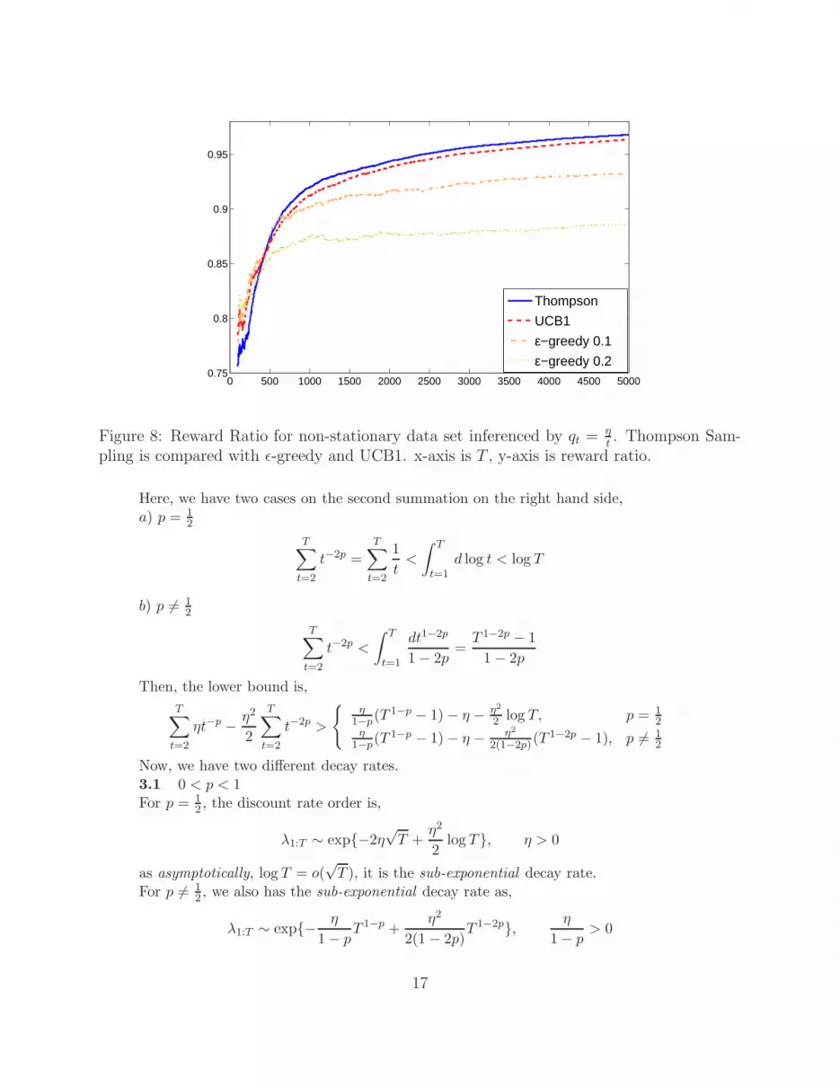
Non-Stationary Distribution

Here, for the modeling, we set δt =0.1t. We may show that the covariance matrix

for parameter generated from this model will be unbounded; thus the samples arenon-stationary. Figure(7) illustrate the parameter choice for power function η

tand η

t2.

Obviously, ηthas better average reward as the data is generated from this function form.

As same as for stationary distribution, ηt2

has larger range for the parameter choiceas it decays slower. In figures(8,9), we find that Thompson Sampling is better thanUCB1 with larger margin. It is mainly because that the approximate inference for the

12

0 500 1000 1500 2000 2500 3000 3500 4000 4500 50000.75

0.8

0.85

0.9

0.95

ThompsonUCB1ε−greedy 0.1ε−greedy 0.2

Figure 4: Reward Ratio for stationary data set inferenced by qt =η

t. Thompson Sampling

is compared with ǫ-greedy and UCB1. x-axis is T , y-axis is reward ratio.

non-stationary samples are quite accurate; and the data are non-stationary. As sameas before, ǫ-greedy is much more worse. For the comparison between logistic regressionand dynamic logistic regression in our non-linear and non-stationary dynamic system,in Figure(10) it ends up better result by dynamic logistic regression as our approximateinference is able to adapt to the dynamics of the underlying distributions; while logisticregression assumes that the parameters are static and stationary.

6 Discussion and Further work

Let’s take a close look at the posterior mean and covariance update again.From Eq.(9), compared to logistic regression, we have,

ut = ut−1 +1

λtΣt−1gt, gt ∈

∂ log P (zt|βt))∂β

here, 1λt

= 1 + qt is the adaptive step size for the stochastic gradient descent formean ut. This step size is adaptive to the underlying change of parameter distributioncharacterized by Qt = qtΣt−1.

For the Hessian updates from Eq.(11),

Ht = λtHt−1 − θt(1− θt)xt · xTt

Compared to logistic regression, the hessian(observed information) is reduced by λt =1

1+qt< 1 according to underlying distribution changes Qt.

13

0 500 1000 1500 2000 2500 3000 3500 4000 4500 50000

0.02

0.04

0.06

0.08

0.1

0.12

0.14

0.16

0.18

0.2

ThompsonUCB1ε−greedy 0.1ε−greedy 0.2

Figure 5: Average Regret for stationary data set inferenced by qt =η

t. Thompson Sampling

is compared with ǫ-greedy and UCB1. x-axis is T , y-axis is regret.

Thus, our approximate inference is able to adapt to exploration and exploitationtrade-off. When the sample distribution changes quickly(qt in larger order), the dis-count factor decays quickly to 0, and the observed information from the previoussamples diminishes, then it needs a larger step size to encourage exploration in pa-rameter space and consequently search space for the expected posterior rewards withhigher uncertainty. If the sample distribution evolves smoothly (qt in smaller order),the discount factor decays to the lower bound, information shrinkage is less heavy, itends up with smaller step size to encourage exploitation.

For further work, we are interested in finding real applications with dynamic systemfor our Thompson Sampling. In additional to learn Qt, another possible extension isto study more complex dynamic system such as,

βt = Atβt−1 + ǫt, ǫt ∼ N (0, Qt)

and discuss the corresponding exploration and exploitation trade-off.

A Decay Rates Analysis

Here, we provide a detailed analysis of the discount decay rates under different powerand exponential functions.

A.1 Power Function Family

For the power function, the decay rate orders are discussed here for different p.1. p = 0.

14

102

103

0

0.02

0.04

0.06

0.08

0.1

0.12

0.14

0.16

0.18

0.2

Logistic RegressionDynamic System

Figure 6: Regrets for stationary data set by Thompson Sampling. The dynamic logisticregression is compared with logistic regression for the same stationary data. x-axis is T ,y-axis is regret.

Here, λt =1

1+η< 1 is constant; the discount factor,

λ1:T = (1 + η)−(T−1) = (1 + η) exp{−(log(1 + η))T}, p = 0, η > 0 (20)

and log(1 + η) > 0, thus, we have the exponential decay rate.2. p = 1.

First, by the integration,∫

log(1 +η

t) dt = η log(t+ η) + t log(1 +

η

t)

we have the upper bound,

T∑

t=2

log(1 +η

t) <

∫ T

1log(1 +

η

t) dt < η log(T + η) + T log(1 +

η

T)

and the lower bound,

T∑

t=2

log(1 +η

t) >

∫ T

1log(1 +

η

t) dt− log(1 + η)

Thus, the summation is in the order of,

T∑

t=2

log(1 +η

t) ∼ η log(T + η) + T log(1 +

η

T)

15

10−2

10−1

100

101

0.8

0.82

0.84

0.86

0.88

0.9

0.92

0.94

0.96

0.98

1

η/t

η/t2

Figure 7: Model selection Rewards for non-stationary data set. Reward Ratio for differentparameters η of two power functions η

tand η

t2, used to do model selection. x-axis is η, y-axis

is reward ratio.

Then, the decay rate is in the order,

λ1:T ∼ exp{−η log(T + η)− T log(1 +η

T)}, η > 0

For sufficient large T , asymptotically, we have,

T log(1 +η

T) → η

Consequently, the asymptotical power law decay rate order is,

λ1:T ∼ exp{−η log(T + η)} = (T + η)−η , p = 1, η > 0 (21)

3. p > 0, p 6= 1.First, we have the inequalities,

ηt−p − η2

2t−2p < log(1 + ηt−p) < ηt−p

Then, the summation is upper bounded by,

T∑

t=2

ηt−p < η

∫ T

t=1

dt1−p

1− p= η

T 1−p − 1

1− p

And lower bounded as,

T∑

t=2

ηt−p − η2

2

T∑

t=2

t−2p > η

∫ T

t=1

dt1−p

1− p− η − η2

2

T∑

t=2

t−2p

16

0 500 1000 1500 2000 2500 3000 3500 4000 4500 50000.75

0.8

0.85

0.9

0.95

Thompson

UCB1

ε−greedy 0.1

ε−greedy 0.2

Figure 8: Reward Ratio for non-stationary data set inferenced by qt =η

t. Thompson Sam-

pling is compared with ǫ-greedy and UCB1. x-axis is T , y-axis is reward ratio.

Here, we have two cases on the second summation on the right hand side,a) p = 1

2

T∑

t=2

t−2p =T∑

t=2

1

t<

∫ T

t=1d log t < log T

b) p 6= 12

T∑

t=2

t−2p <

∫ T

t=1

dt1−2p

1− 2p=

T 1−2p − 1

1− 2p

Then, the lower bound is,

T∑

t=2

ηt−p − η2

2

T∑

t=2

t−2p >

{

η1−p

(T 1−p − 1)− η − η2

2 log T, p = 12

η1−p

(T 1−p − 1)− η − η2

2(1−2p)(T1−2p − 1), p 6= 1

2

Now, we have two different decay rates.3.1 0 < p < 1For p = 1

2 , the discount rate order is,

λ1:T ∼ exp{−2η√T +

η2

2log T}, η > 0

as asymptotically, log T = o(√T ), it is the sub-exponential decay rate.

For p 6= 12 , we also has the sub-exponential decay rate as,

λ1:T ∼ exp{− η

1− pT 1−p +

η2

2(1 − 2p)T 1−2p}, η

1− p> 0

17

0 500 1000 1500 2000 2500 3000 3500 4000 4500 50000.02

0.04

0.06

0.08

0.1

0.12

0.14

0.16

0.18

0.2

ThompsonUCB1ε−greedy 0.1ε−greedy 0.2

Figure 9: Average Regret for non-stationary data set inferenced by qt = η

t. Thompson

Sampling is compared with ǫ-greedy and UCB1. x-axis is T , y-axis is regret.

Furthermore, the asymptotical sub-exponential rate,

λ1:T ∼ exp{− η

1− pT 1−p}, 0 < p < 1, η > 0 (22)

3.2 p > 1

λ1:T ∼ exp{ η

p − 1T 1−p − η2

2(2p − 1)T 1−2p}

∼ exp{ η

p− 1T 1−p}, η

p− 1> 0

Asymptotically, the power law decay rate is in the order,

λ1:T ∼ η

p− 1T 1−p, p > 1, η > 0 (23)

Here, as T → ∞, we have the lower bound for the discount decay as,

λ1:T > exp{−η1 − T 1−p

p− 1} → exp{− η

p− 1}, p > 1, η > 0 (24)

4. p < 0.First, we have,

log(1 + ηt−p) = log(ηt−p) + log(1 +1

ηtp)

18

102

103

0.02

0.04

0.06

0.08

0.1

0.12

0.14

0.16

0.18

0.2

Logistic RegressionDynamic System

Figure 10: Regrets for non-stationary data set by Thompson Sampling. The dynamic logisticregression is compared with logistic regression for the same non-stationary data. x-axis isT , y-axis is regret.

The second term is equivelent to the case where −p > 0, asymptotically, the summationis in the order of, for p 6= −1,

T∑

t=2

log(1 +1

ηtp) ∼ T 1+p − 1

η(1 + p), η > 0, p < 0

for p = −1,

T∑

t=2

log(1 +1

ηt−1) ∼ 1

ηlog(T +

1

η), η > 0

By the integration,

T∑

t=2

log t ∼∫ T

t=1d(t log t− t) ∼ T log T − T

then, for the first term, the summation,

T∑

t=2

log(ηt−p) =

T∑

t=2

log η − p

T∑

t=2

log t ∼ −pT log T + pT + T log η

Now, we show the asymptotically decay rate is in the order of sup-exponential as,

λ1:T ∼ exp{pT log T}, p < 0 (25)

19

4.1 p = −1

λ1:T ∼ exp{pT log T − pT − T log η − 1

ηlog(T +

1

η)} ∼ exp{pT log T}

4.2 p = −12

λ1:T ∼ exp{pT log T − pT − T log η − T 1+p

η(1 + p)} ∼ exp{pT log T}

4.3 0 < −p < 1, p 6= −12 ,−p > 1

λ1:T ∼ exp{pT log T − pT − T log η − T 1+p − 1

η(1 + p)} ∼ exp{pT log T}

A.2 Exponential Function Family

For the exponential function we analyze the different decay rates under different con-ditions for γ.1. γ = 1

This case is the same as in the case 1 of power function, it has the same exponentialdecay in Eq.(20).2. 0 < γ < 1

First, we have the inequalities,

ηγt − η2

2< log(1 + ηγt) < ηγt

and the upper bound,

η

T∑

t=2

γt < η1− γT+1

1− γ

the lower bound,

T∑

t=2

log(1 + ηγt) > η(1− γT+1

1− γ− 1− γ)− η2

2(1− γ2(T+1)

1− γ2− 1− γ2)

as γ2T = o(γT ), the discount decay is in the asymptotical order,

λ1:T ∼ exp{ ηγ

1− γγT }

Asymptotoically, we have the exponential decay rate,

λ1:T ∼ ηγ

1− γγT , 0 < γ < 1, η > 0 (26)

Here, as T → ∞, we have a lower bound for the discount decay,

λ1:T > exp{ηγT+1 − 1

1− γ} → exp{− η

1− γ}, 0 < γ < 1, η > 0 (27)

20

3. γ > 1First, we have,

log(1 + ηγt) = log(ηγt) + log(1 +1

η(1

γ)t), 0 <

1

γ< 1

asymptotically, the summation of second term,

T∑

t=2

log(1 +1

η(1

γ)t) ∼ γ − γ−T

η(γ − 1)

the first term,

T∑

t

log(ηγt) =T∑

t=2

log η + log γT∑

t=2

t = (T − 1) log η +(T − 1)(T + 2)

2log γ

Then, the discount decay rate,

λ1:T ∼ exp{−(log γ)T 2 − (log η)T +γ−T

η(γ − 1)}

Thus, asymptotically, we have the super-exponential order of decay rate,

λ1:T ∼ exp{−(log γ)T 2}, γ > 1 (28)

21

References

[ACBF02] Peter Auer, Nicolo Cesa-Bianchi, and Paul Fischer. Finite-time analysisof the multiarmed bandit problem. Machine Learning, 47:235 – 256, 2002.

[CL11] Olivier Chapelle and Lihong Li. An empirical evaluation of thompson sam-pling. In Advances in Neural Information Processing Systems 24 (NIPS-11), 2011.

[Git79] J. C. Gittins. Bandit processes and dynamic allocation indices. Journalof the Royal Statistical Society, 41:148–177, 1979.

[Kal60] Rudolph Emil Kalman. A new approach to linear filtering and predictionproblems. Transactions of the ASME–Journal of Basic Engineering, 82:35–45, 1960.

[LCLS10] Lihong Li, Wei Chu, John Langford, and Robert E. Schapire. A contextual-bandit approach to personalized news article recommendation. In In Pro-ceedings of the Nineteenth International Conference on World Wide Web(WWW-10), page 661670, 2010.

[MKLL12] Benedict C. May, Nathan Korda, Anthony Lee, and David S. Leslie. Op-timistic bayesian sampling in contextual-bandit problems. Journal of Ma-chine Learning Research, 13:2069–2106, 2012.

[MRMB12] Tyler H. McCormick, Adrian E. Raftery, David Madigan, and Randall S.Burd. Dynamic logistic regression and dynamic model averaging for binaryclassification. Biometrics, 68:23–30, 2012.

[PR99] William D. Penny and Stephen J. Roberts. Dynamic logistic regression.In International Joint Conference on Neural Networks (IJCNN ’99), pages1562 – 1567, July 1999.

[SM50] Jack Sherman and Winifred J. Morrison. Adjustment of an inverse matrixcorresponding to a change in one element of a given matrix. Annals ofMathematical Statistics, 21:124–127, 1950.

[Tho33] William R. Thompson. On the likelihood that one unknown probabil-ity exceeds another in view of the evidence of two samples. Biometrika,25:285294, 1933.

[WH97] Mike West and P. Jeff Harrison. Bayesian forecasting and dynamic models.Springer Series in Statistics, 2:618, 1997.

[WHsM85] Mike West, P. Jeff Harrison, and Helio s. Migon. Dynamic generalizedlinear models and bayesian forecasting. Journal of the American StatisticalAssociation, 80, 1985.

22