exponential growth and decay

2Exponential Growth and Decay

The exponential function is one of the most important andwidely occurring functions in physics and biology. In biologyit may describe the growth of bacteria or animal populations,the decrease of the number of bacteria in response to a ster-ilization process, the growth of a tumor, or the absorption orexcretion of a drug. (Exponential growth cannot continue for-ever because of limitations of nutrients, etc.) Knowledge ofthe exponential function makes it easier to understand birthand death rates, even when they are not constant. In physics,the exponential function describes the decay of radioactivenuclei, the emission of light by atoms, the absorption of lightas it passes through matter, the change of voltage or currentin some electrical circuits, the variation of temperature withtime as a warm object cools, and the rate of some chemicalreactions.

In this book, the exponential function will be needed todescribe certain probability distributions, the concentrationratio of ions across a cell membrane, the flow of soluteparticles through membranes, the decay of a signal travel-ing along a nerve axon, and the return of some physiologicvariables to their equilibrium values after they have beendisturbed.

Because the exponential function is so important, and be-cause we have seen many students who did not understandit even after having been exposed to it, the chapter startswith a gentle introduction to exponential growth (Sect. 2.1)and decay (Sect. 2.2). Section 2.3 shows how to analyze ex-ponential data using semilogarithmic graph paper. The nextsection shows how to use semilogarithmic graph paper tofind instantaneous growth or decay rates when the rate varies.Some would argue that the availability of computer programsthat automatically produce logarithmic scales for plots makesthese sections unnecessary. We feel that intelligent use ofsemilogarithmic and logarithmic (log–log) plots requires anunderstanding of the basic principles.

Variable rates are described in Sect. 2.4. Clearance, dis-cussed in Sect. 2.5, is an exponential decay process that isimportant in physiology. Microbiologists often grow cellsin a chemostat, described in Sect. 2.6. Sometimes there are

competing paths for exponential removal of a substance:multiple decay paths are introduced in Sect. 2.7. A very ba-sic and simple model for many processes is the combinationof input at a fixed rate accompanied by exponential decay,described in Sect. 2.8. Sometimes a substance exists in twoforms, each with its own decay rate. One then must fit two ormore exponentials to the set of data, as shown in Sect. 2.9.

Section 2.10 discusses the logistic equation, one possiblemodel for a situation in which the growth rate decreases asthe amount of substance increases. The chapter closes witha section on power–law relationships. While not exponen-tial, they are included because data analysis can be done withlog–log graph paper, a technique similar to that for semilogpaper. If you feel mathematically secure, you may wish toskim the first four sections, but you will probably find therest of the chapter worth reading.

2.1 Exponential Growth

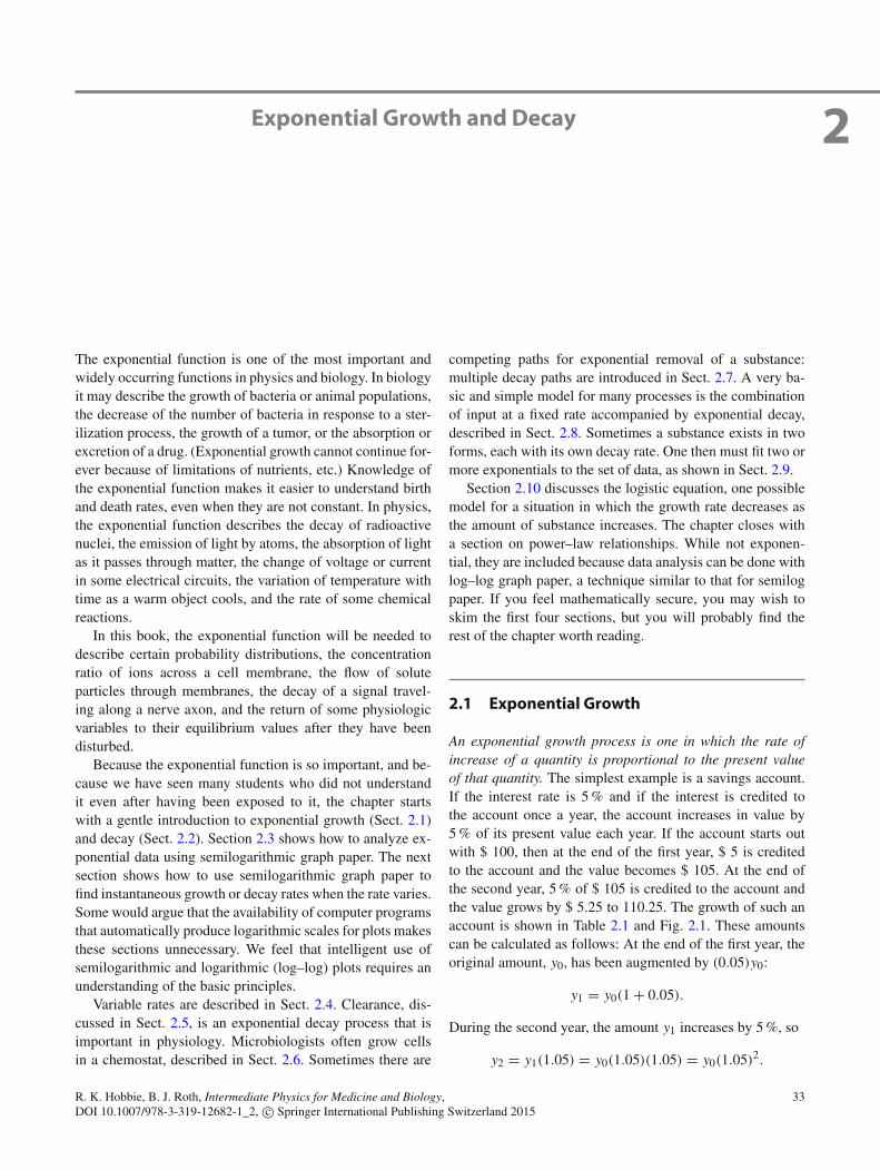
An exponential growth process is one in which the rate ofincrease of a quantity is proportional to the present valueof that quantity. The simplest example is a savings account.If the interest rate is 5 % and if the interest is credited tothe account once a year, the account increases in value by5 % of its present value each year. If the account starts outwith $ 100, then at the end of the first year, $ 5 is creditedto the account and the value becomes $ 105. At the end ofthe second year, 5 % of $ 105 is credited to the account andthe value grows by $ 5.25 to 110.25. The growth of such anaccount is shown in Table 2.1 and Fig. 2.1. These amountscan be calculated as follows: At the end of the first year, theoriginal amount, y0, has been augmented by (0.05)y0:

y1 = y0(1 + 0.05).

During the second year, the amount y1 increases by 5 %, so

y2 = y1(1.05) = y0(1.05)(1.05) = y0(1.05)2.

R. K. Hobbie, B. J. Roth, Intermediate Physics for Medicine and Biology, 33DOI 10.1007/978-3-319-12682-1_2, c© Springer International Publishing Switzerland 2015

34 2 Exponential Growth and Decay

Table 2.1 Growth of a savings account earning 5 % interest com-pounded annually, when the initial investment is $ 100

Year Amount ($) Year Amount ($) Year Amount ($)

1 105.00 10 162.88 100 1.31 × 104

2 110.25 20 265.33 200 1.73 × 106

3 115.76 30 432.19 300 2.27 × 108

4 121.55 40 704.00 400 2.99 × 1010

5 127.63 50 1146.74 500 3.93 × 1012

6 134.01 60 1867.92 600 5.17 × 1014

7 140.71 70 3042.64 700 6.80 × 1016

8 147.75 80 4956.14 800 8.94 × 1018

9 155.13 90 8073.04 900 1.18 × 1021

900

800

700

600

500

400

300

200

100

0

Val

ue (

dolla

rs)

50403020100

Time (years)

Fig. 2.1 The amount in a savings account after t years, when theamount is compounded annually at 5 % interest

After t years, the amount in the account is

yt = y0(1.05)t .

In general, if the growth rate is b per compounding period,the amount after t periods is

yt = y0(1 + b)t . (2.1)

It is possible to keep the same annual growth (interest)rate, but to compound more often than once a year. Ta-ble 2.2 shows the effect of different compounding intervalson the amount, when the interest rate is 5 %. The last twocolumns, for monthly compounding and for “instant inter-est,” are listed to the nearest tenth of a cent to show the slightdifference between them.

The table entries were calculated in the following way:Suppose that compounding is done N times a year. In t years,the number of compoundings is Nt . If the annual fractional

Table 2.2 Amount of an initial investment of $ 100 at 5 % annualinterest, with different methods of compounding

Month Annual Semiannual Quarterly Monthly Instant($) ($) ($) ($) ($)

0 100.00 100.00 100.00 100.000 100.0001 100.00 100.00 100.00 100.417 100.4182 100.00 100.00 100.00 100.835 100.8373 100.00 100.00 101.25 101.255 101.2584 100.00 100.00 101.25 101.677 101.6815 100.00 100.00 101.25 102.101 102.1056 100.00 102.50 102.52 102.526 102.5327 100.00 102.50 102.52 102.953 102.9608 100.00 102.50 102.52 103.382 103.3909 100.00 102.50 103.80 103.813 103.82110 100.00 102.50 103.80 104.246 104.25511 100.00 102.50 103.80 104.680 104.69012 105.00 105.06 105.09 105.116 105.127

Table 2.3 Numerical examples of the convergence of (1 + b/N)N toeb as N becomes large

N b = 1 b = 0.0510 2.594 1.0511

100 2.705 1.05131000 2.717 1.0513

eb 2.718 1.0513

rate of increase is b, the increase per compounding is b/N .For 6 months at 5 % (b = 0.05), the increase is 2.5, for 3months it is 1.25, etc. The amount after t units of time (years)is, in analogy with Eq. 2.1,

y = y0 (1 + b/N)Nt . (2.2)

Recall (refer to Appendix C) that (a)bc = (ab)c. Theexpression for y can be written as

y = y0

[(1 + b/N)N

]t. (2.3)

Most calculus textbooks show that the quantity

(1 + b/N)N → eb

as N becomes very large. (Rather than proving this fact here,we give numerical examples in Table 2.3 for two differentvalues of b.) Therefore, Eq. 2.3 can be rewritten as

y = y0ebt = y0 exp(bt). (2.4)

(The exp notation is used when the argument is compli-cated.) To calculate the amount for instant interest, it isnecessary only to multiply the fractional growth rate perunit time b by the length of the time interval and then lookup the exponential function of this amount in a table orevaluate it with a computer or calculator. The number e isapproximately equal to 2.71828 . . . and is called the base ofthe natural logarithms. Like π (3.14159 . . . ), e has a longhistory (Maor 1994).

2.2 Exponential Decay 35

8

7

6

5

4

3

2

1

0

y=et

-2 -1 0 1 2

t

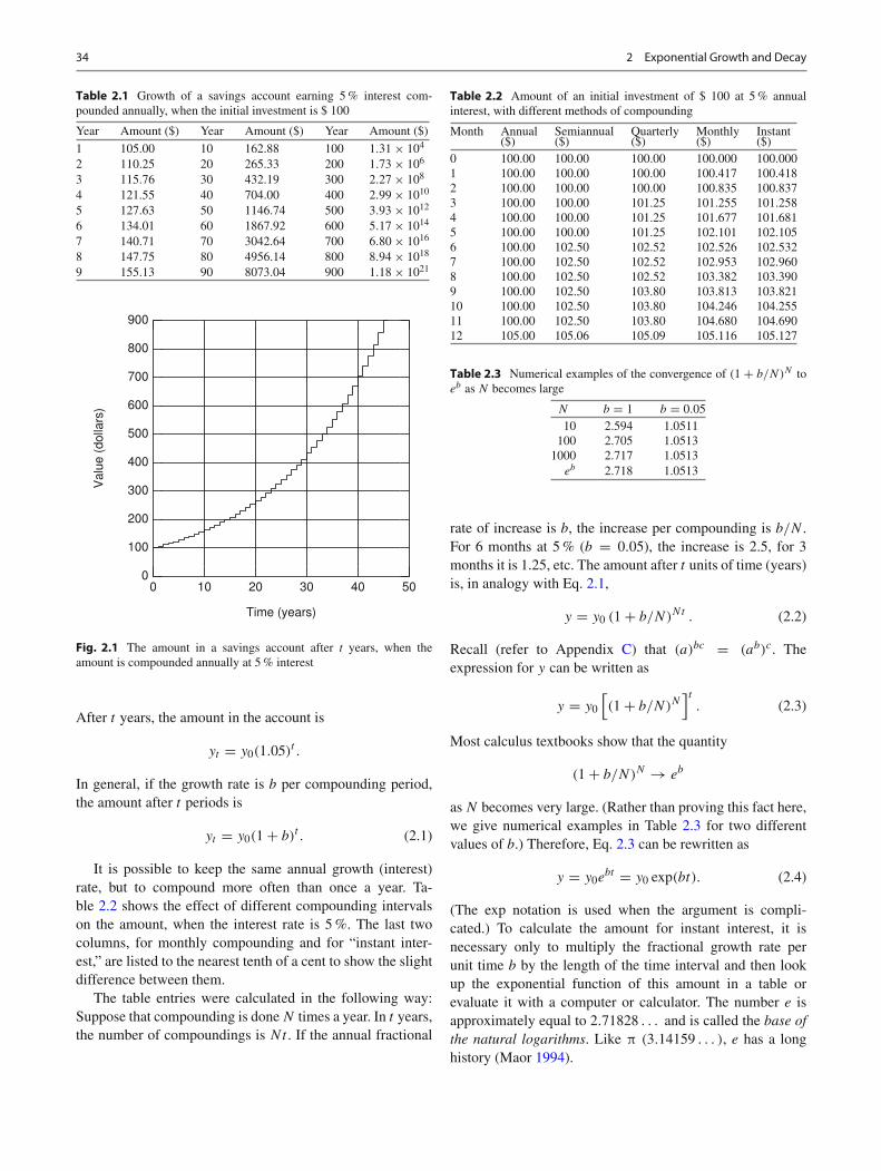
Fig. 2.2 A graph of the exponential function y = et

The exponential function is plotted in Fig. 2.2. (The mean-ing of negative values of t will be considered in the nextsection.) This function increases more and more rapidly as t

increases. This is expected, since the rate of growth is alwaysproportional to the present amount. This is also reflected inthe following property of the exponential function:

d

dt

(ebt)

= bebt . (2.5)

This means that the function y = y0ebt has the property that

dy

dt= by. (2.6)

Any constant multiple of the exponential function ebt has theproperty that its rate of growth is b times the function itself.Whenever we see the exponential function, we know that itsatisfies Eq. 2.6. Equation 2.6 is an example of a differen-tial equation. If you learn how to solve only one differentialequation, let it be Eq. 2.6. Whenever we have a problem inwhich the growth rate of something is proportional to thepresent amount, we can expect to have an exponential solu-tion. Notice that for time intervals t that are not too large,Eq. 2.6 implies that �y = (b�t)y. This again says that theincrease in y is proportional to y itself.

The independent variable in this discussion has been t . Itcan represent time, in which case b is the fractional growthrate per unit time; distance, in which case b is the fractionalgrowth per unit distance; or something else. We could, ofcourse, use another symbol such as x for the independentvariable, in which case we would have dy/dx = by, y =y0e

bx .

1.0

0.8

0.6

0.4

0.2

0.0

Fra

ctio

n R

emai

ning

121086420

t, hours

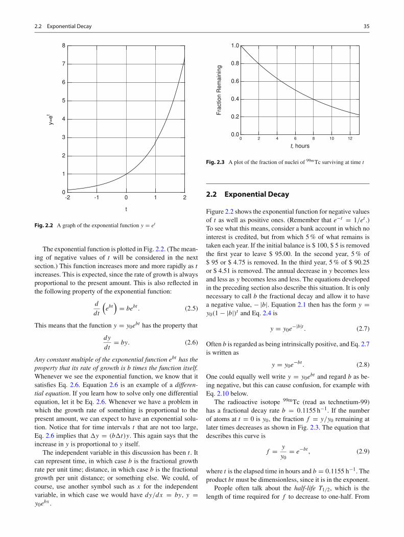
Fig. 2.3 A plot of the fraction of nuclei of 99mTc surviving at time t

2.2 Exponential Decay

Figure 2.2 shows the exponential function for negative valuesof t as well as positive ones. (Remember that e−t = 1/et .)To see what this means, consider a bank account in which nointerest is credited, but from which 5 % of what remains istaken each year. If the initial balance is $ 100, $ 5 is removedthe first year to leave $ 95.00. In the second year, 5 % of$ 95 or $ 4.75 is removed. In the third year, 5 % of $ 90.25or $ 4.51 is removed. The annual decrease in y becomes lessand less as y becomes less and less. The equations developedin the preceding section also describe this situation. It is onlynecessary to call b the fractional decay and allow it to havea negative value, − |b|. Equation 2.1 then has the form y =y0(1 − |b|)t and Eq. 2.4 is

y = y0e−|b|t . (2.7)

Often b is regarded as being intrinsically positive, and Eq. 2.7is written as

y = y0e−bt . (2.8)

One could equally well write y = y0ebt and regard b as be-

ing negative, but this can cause confusion, for example withEq. 2.10 below.

The radioactive isotope 99mTc (read as technetium-99)has a fractional decay rate b = 0.1155 h−1. If the numberof atoms at t = 0 is y0, the fraction f = y/y0 remaining atlater times decreases as shown in Fig. 2.3. The equation thatdescribes this curve is

f = y

y0= e−bt , (2.9)

where t is the elapsed time in hours and b = 0.1155 h−1. Theproduct bt must be dimensionless, since it is in the exponent.

People often talk about the half-life T1/2, which is thelength of time required for f to decrease to one-half. From


inspection of Fig. 2.3, the half-life is 6 h. This can also bedetermined from Eq. 2.9:

0.5 = e−bT1/2 .

From a table of exponentials, one finds that e−x = 0.5 whenx = 0.69315. This leads to the very useful relationshipbT1/2 = 0.693 or

T1/2 = 0.693

b. (2.10)

For the case of 99mTc, the half-life is T1/2 = 0.693/0.1155 =6 h.

One can also speak of a doubling time if the exponent ispositive. In that case, 2 = ebT2 , from which

T2 = 0.693

b. (2.11)

2.3 Semilog Paper

A special kind of graph paper, called semilog paper, makesthe analysis of exponential growth and decay problems muchsimpler. If one takes logarithms (to any base) of Eq. 2.4, onehas

log y = log y0 + bt log e. (2.12)

If the dependent variable is considered to be u = log y, andsince log y0 and log e are constants, this equation is of theform

u = c1 + c2t . (2.13)

The graph of u vs t is a straight line with positive slope if b

is positive and negative slope if b is negative.On semilog paper the vertical axis is marked in a loga-

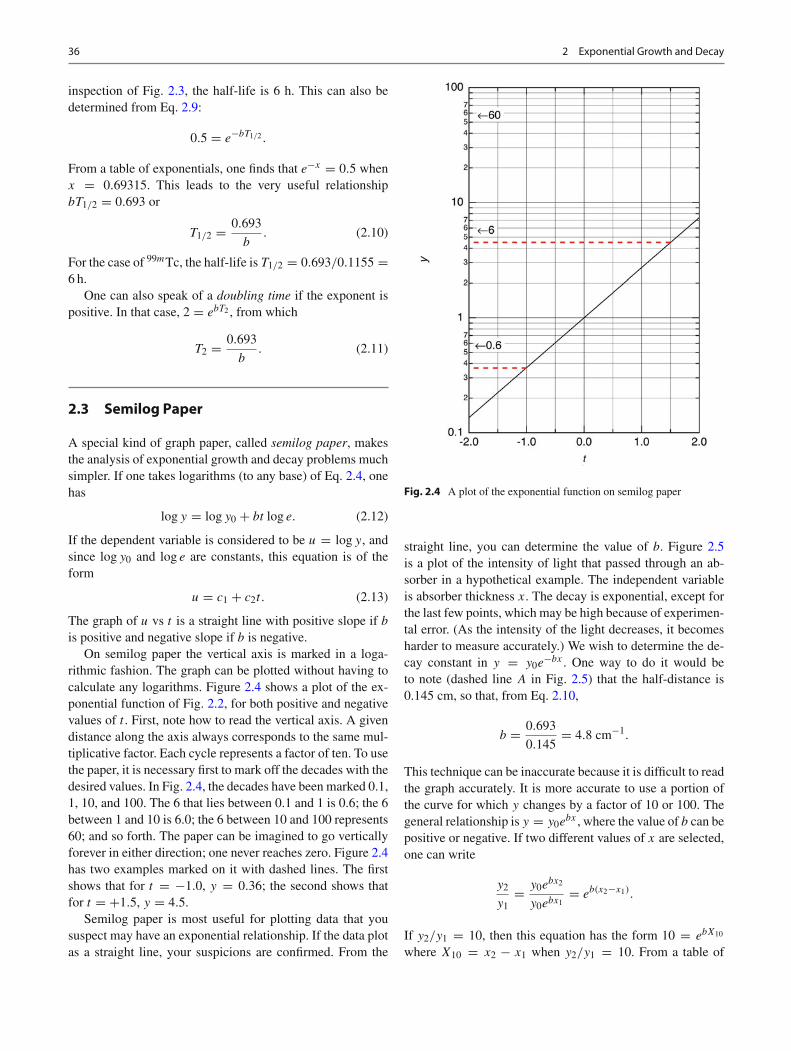
rithmic fashion. The graph can be plotted without having tocalculate any logarithms. Figure 2.4 shows a plot of the ex-ponential function of Fig. 2.2, for both positive and negativevalues of t . First, note how to read the vertical axis. A givendistance along the axis always corresponds to the same mul-tiplicative factor. Each cycle represents a factor of ten. To usethe paper, it is necessary first to mark off the decades with thedesired values. In Fig. 2.4, the decades have been marked 0.1,1, 10, and 100. The 6 that lies between 0.1 and 1 is 0.6; the 6between 1 and 10 is 6.0; the 6 between 10 and 100 represents60; and so forth. The paper can be imagined to go verticallyforever in either direction; one never reaches zero. Figure 2.4has two examples marked on it with dashed lines. The firstshows that for t = −1.0, y = 0.36; the second shows thatfor t = +1.5, y = 4.5.

Semilog paper is most useful for plotting data that yoususpect may have an exponential relationship. If the data plotas a straight line, your suspicions are confirmed. From the

Fig. 2.4 A plot of the exponential function on semilog paper

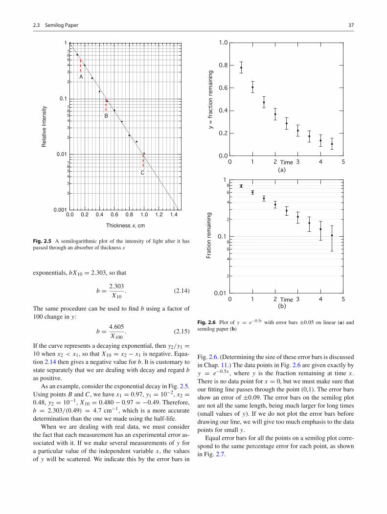
straight line, you can determine the value of b. Figure 2.5is a plot of the intensity of light that passed through an ab-sorber in a hypothetical example. The independent variableis absorber thickness x. The decay is exponential, except forthe last few points, which may be high because of experimen-tal error. (As the intensity of the light decreases, it becomesharder to measure accurately.) We wish to determine the de-cay constant in y = y0e

−bx . One way to do it would beto note (dashed line A in Fig. 2.5) that the half-distance is0.145 cm, so that, from Eq. 2.10,

b = 0.693

0.145= 4.8 cm−1.

This technique can be inaccurate because it is difficult to readthe graph accurately. It is more accurate to use a portion ofthe curve for which y changes by a factor of 10 or 100. Thegeneral relationship is y = y0e

bx , where the value of b can bepositive or negative. If two different values of x are selected,one can write

y2

y1= y0e

bx2

y0ebx1= eb(x2−x1).

If y2/y1 = 10, then this equation has the form 10 = ebX10

where X10 = x2 − x1 when y2/y1 = 10. From a table of

2.3 Semilog Paper 37

0.001

2

3

4567

0.01

2

3

4567

0.1

2

3

4567

1R

elat

ive

Inte

nsity

1.41.21.00.80.60.40.20.0

Thickness x, cm

A

B

C

Fig. 2.5 A semilogarithmic plot of the intensity of light after it haspassed through an absorber of thickness x

exponentials, bX10 = 2.303, so that

b = 2.303

X10. (2.14)

The same procedure can be used to find b using a factor of100 change in y:

b = 4.605

X100. (2.15)

If the curve represents a decaying exponential, then y2/y1 =10 when x2 < x1, so that X10 = x2 − x1 is negative. Equa-tion 2.14 then gives a negative value for b. It is customary tostate separately that we are dealing with decay and regard b

as positive.As an example, consider the exponential decay in Fig. 2.5.

Using points B and C, we have x1 = 0.97, y1 = 10−2, x2 =0.48, y2 = 10−1, X10 = 0.480 − 0.97 = −0.49. Therefore,b = 2.303/(0.49) = 4.7 cm−1, which is a more accuratedetermination than the one we made using the half-life.

When we are dealing with real data, we must considerthe fact that each measurement has an experimental error as-sociated with it. If we make several measurements of y fora particular value of the independent variable x, the valuesof y will be scattered. We indicate this by the error bars in

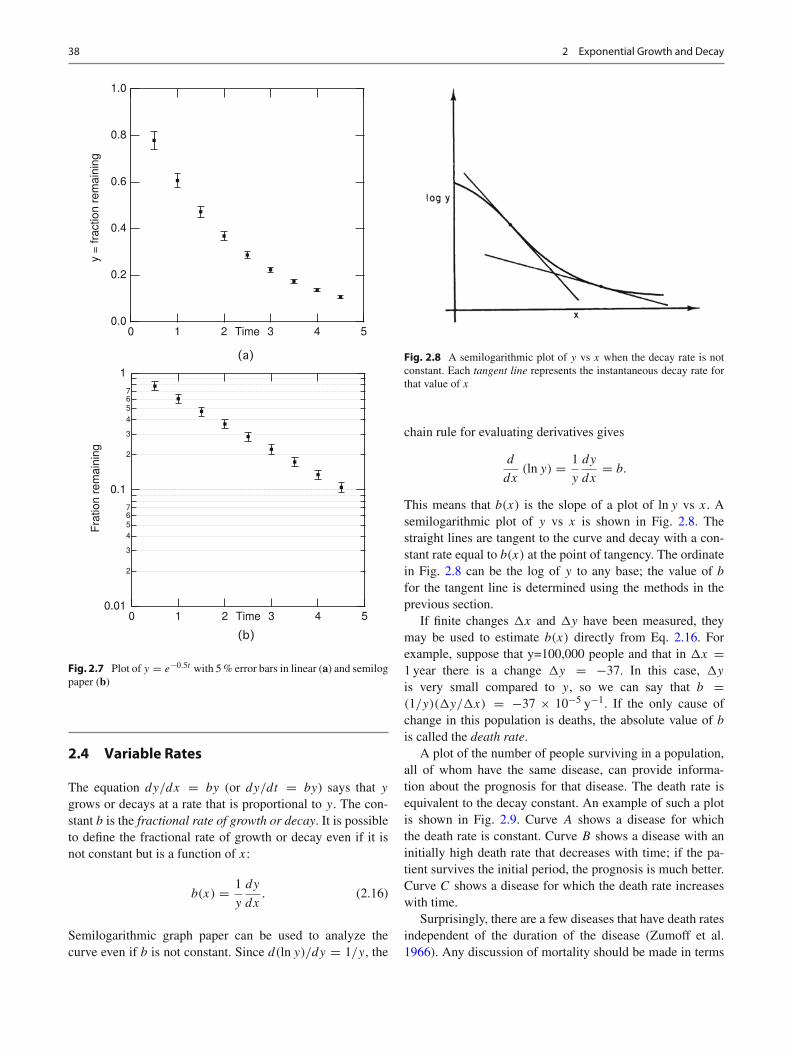
Fig. 2.6 Plot of y = e−0.5t with error bars ±0.05 on linear (a) andsemilog paper (b)

Fig. 2.6. (Determining the size of these error bars is discussedin Chap. 11.) The data points in Fig. 2.6 are given exactly byy = e−0.5x , where y is the fraction remaining at time x.There is no data point for x = 0, but we must make sure thatour fitting line passes through the point (0,1). The error barsshow an error of ±0.09. The error bars on the semilog plotare not all the same length, being much larger for long times(small values of y). If we do not plot the error bars beforedrawing our line, we will give too much emphasis to the datapoints for small y.

Equal error bars for all the points on a semilog plot corre-spond to the same percentage error for each point, as shownin Fig. 2.7.


1.0

0.8

0.6

0.4

0.2

0.0

y =

frac

tion

rem

aini

ng

543210 Time

0.01

2

3

4567

0.1

2

3

4567

1

Fra

tion

rem

aini

ng

543210 Time

Fig. 2.7 Plot of y = e−0.5t with 5 % error bars in linear (a) and semilogpaper (b)

2.4 Variable Rates

The equation dy/dx = by (or dy/dt = by) says that y

grows or decays at a rate that is proportional to y. The con-stant b is the fractional rate of growth or decay. It is possibleto define the fractional rate of growth or decay even if it isnot constant but is a function of x:

b(x) = 1

y

dy

dx. (2.16)

Semilogarithmic graph paper can be used to analyze thecurve even if b is not constant. Since d(ln y)/dy = 1/y, the

Fig. 2.8 A semilogarithmic plot of y vs x when the decay rate is notconstant. Each tangent line represents the instantaneous decay rate forthat value of x

chain rule for evaluating derivatives gives

d

dx(ln y) = 1

y

dy

dx= b.

This means that b(x) is the slope of a plot of ln y vs x. Asemilogarithmic plot of y vs x is shown in Fig. 2.8. Thestraight lines are tangent to the curve and decay with a con-stant rate equal to b(x) at the point of tangency. The ordinatein Fig. 2.8 can be the log of y to any base; the value of b

for the tangent line is determined using the methods in theprevious section.

If finite changes �x and �y have been measured, theymay be used to estimate b(x) directly from Eq. 2.16. Forexample, suppose that y=100,000 people and that in �x =1 year there is a change �y = −37. In this case, �y

is very small compared to y, so we can say that b =(1/y)(�y/�x) = −37 × 10−5 y−1. If the only cause ofchange in this population is deaths, the absolute value of b

is called the death rate.A plot of the number of people surviving in a population,

all of whom have the same disease, can provide informa-tion about the prognosis for that disease. The death rate isequivalent to the decay constant. An example of such a plotis shown in Fig. 2.9. Curve A shows a disease for whichthe death rate is constant. Curve B shows a disease with aninitially high death rate that decreases with time; if the pa-tient survives the initial period, the prognosis is much better.Curve C shows a disease for which the death rate increaseswith time.

Surprisingly, there are a few diseases that have death ratesindependent of the duration of the disease (Zumoff et al.1966). Any discussion of mortality should be made in terms

2.4 Variable Rates 39

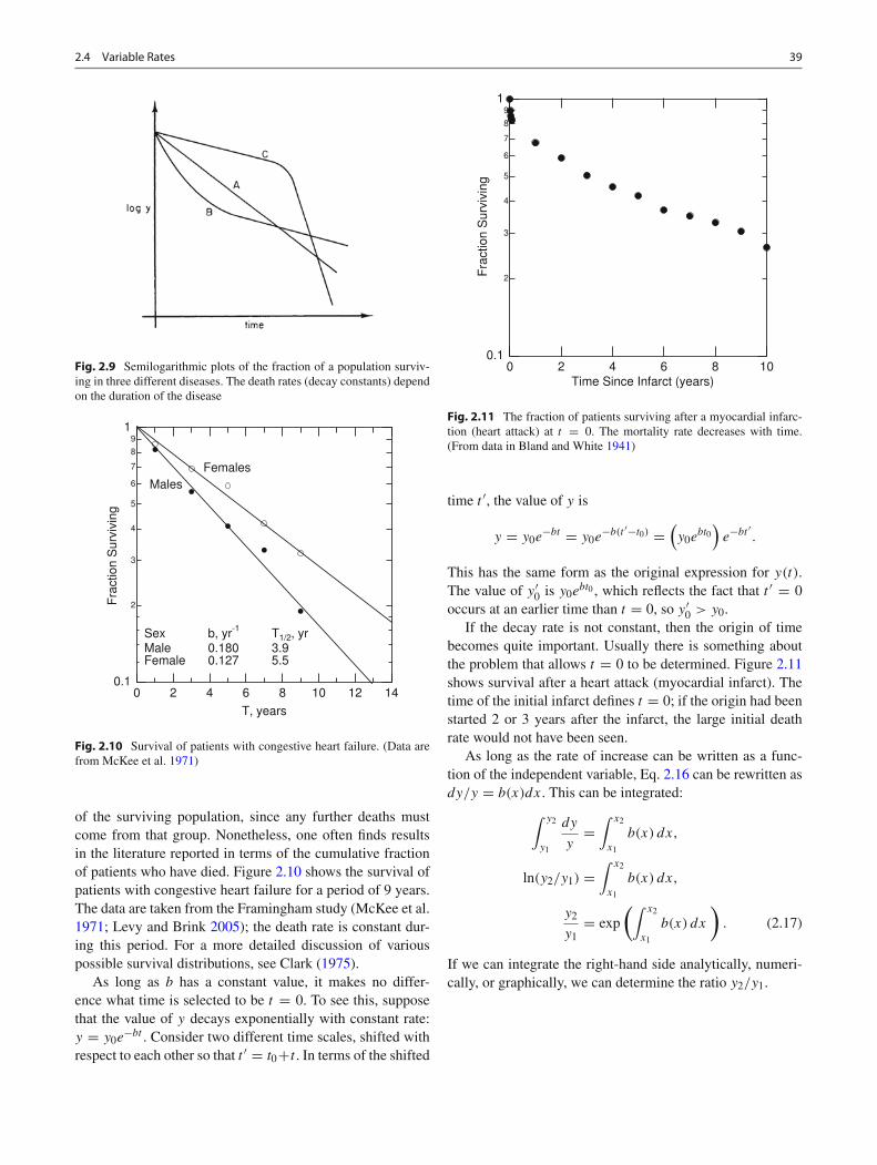
Fig. 2.9 Semilogarithmic plots of the fraction of a population surviv-ing in three different diseases. The death rates (decay constants) dependon the duration of the disease

0.1

2

3

4

5

6

7

8

91

Fra

ctio

n S

urvi

ving

14121086420

T, years

MalesFemales

Sex b, yr-1 T1/2, yrMale 0.180 3.9Female 0.127 5.5

Fig. 2.10 Survival of patients with congestive heart failure. (Data arefrom McKee et al. 1971)

of the surviving population, since any further deaths mustcome from that group. Nonetheless, one often finds resultsin the literature reported in terms of the cumulative fractionof patients who have died. Figure 2.10 shows the survival ofpatients with congestive heart failure for a period of 9 years.The data are taken from the Framingham study (McKee et al.1971; Levy and Brink 2005); the death rate is constant dur-ing this period. For a more detailed discussion of variouspossible survival distributions, see Clark (1975).

As long as b has a constant value, it makes no differ-ence what time is selected to be t = 0. To see this, supposethat the value of y decays exponentially with constant rate:y = y0e

−bt . Consider two different time scales, shifted withrespect to each other so that t ′ = t0+t . In terms of the shifted

0.1

2

3

4

5

6

7

8

91

Fra

ctio

n S

urvi

ving

1086420Time Since Infarct (years)

Fig. 2.11 The fraction of patients surviving after a myocardial infarc-tion (heart attack) at t = 0. The mortality rate decreases with time.(From data in Bland and White 1941)

time t ′, the value of y is

y = y0e−bt = y0e

−b(t ′−t0) =(y0e

bt0)

e−bt ′ .

This has the same form as the original expression for y(t).The value of y′

0 is y0ebt0 , which reflects the fact that t ′ = 0

occurs at an earlier time than t = 0, so y′0 > y0.

If the decay rate is not constant, then the origin of timebecomes quite important. Usually there is something aboutthe problem that allows t = 0 to be determined. Figure 2.11shows survival after a heart attack (myocardial infarct). Thetime of the initial infarct defines t = 0; if the origin had beenstarted 2 or 3 years after the infarct, the large initial deathrate would not have been seen.

As long as the rate of increase can be written as a func-tion of the independent variable, Eq. 2.16 can be rewritten asdy/y = b(x)dx. This can be integrated:

∫ y2

y1

dy

y=∫ x2

x1

b(x) dx,

ln(y2/y1) =∫ x2

x1

b(x) dx,

y2

y1= exp

(∫ x2

x1

b(x) dx

). (2.17)

If we can integrate the right-hand side analytically, numeri-cally, or graphically, we can determine the ratio y2/y1.


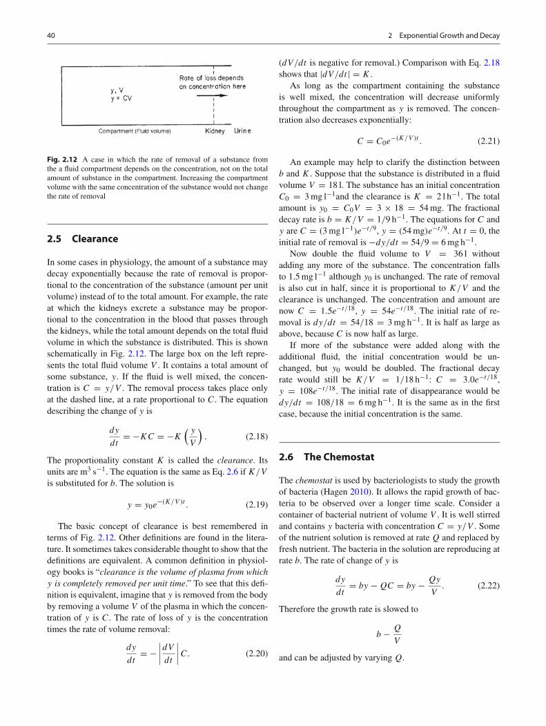
Fig. 2.12 A case in which the rate of removal of a substance fromthe a fluid compartment depends on the concentration, not on the totalamount of substance in the compartment. Increasing the compartmentvolume with the same concentration of the substance would not changethe rate of removal

2.5 Clearance

In some cases in physiology, the amount of a substance maydecay exponentially because the rate of removal is propor-tional to the concentration of the substance (amount per unitvolume) instead of to the total amount. For example, the rateat which the kidneys excrete a substance may be propor-tional to the concentration in the blood that passes throughthe kidneys, while the total amount depends on the total fluidvolume in which the substance is distributed. This is shownschematically in Fig. 2.12. The large box on the left repre-sents the total fluid volume V . It contains a total amount ofsome substance, y. If the fluid is well mixed, the concen-tration is C = y/V . The removal process takes place onlyat the dashed line, at a rate proportional to C. The equationdescribing the change of y is

dy

dt= −KC = −K

( y

V

). (2.18)

The proportionality constant K is called the clearance. Itsunits are m3 s−1. The equation is the same as Eq. 2.6 if K/V

is substituted for b. The solution is

y = y0e−(K/V )t . (2.19)

The basic concept of clearance is best remembered interms of Fig. 2.12. Other definitions are found in the litera-ture. It sometimes takes considerable thought to show that thedefinitions are equivalent. A common definition in physiol-ogy books is “clearance is the volume of plasma from whichy is completely removed per unit time.” To see that this defi-nition is equivalent, imagine that y is removed from the bodyby removing a volume V of the plasma in which the concen-tration of y is C. The rate of loss of y is the concentrationtimes the rate of volume removal:

dy

dt= −

∣∣∣∣dV

dt

∣∣∣∣C. (2.20)

(dV/dt is negative for removal.) Comparison with Eq. 2.18shows that |dV/dt | = K .

As long as the compartment containing the substanceis well mixed, the concentration will decrease uniformlythroughout the compartment as y is removed. The concen-tration also decreases exponentially:

C = C0e−(K/V )t . (2.21)

An example may help to clarify the distinction betweenb and K . Suppose that the substance is distributed in a fluidvolume V = 18 l. The substance has an initial concentrationC0 = 3 mg l−1and the clearance is K = 2 l h−1. The totalamount is y0 = C0V = 3 × 18 = 54 mg. The fractionaldecay rate is b = K/V = 1/9 h−1. The equations for C andy are C = (3 mg l−1)e−t/9, y = (54 mg)e−t/9. At t = 0, theinitial rate of removal is −dy/dt = 54/9 = 6 mg h−1.

Now double the fluid volume to V = 36 l withoutadding any more of the substance. The concentration fallsto 1.5 mg l−1 although y0 is unchanged. The rate of removalis also cut in half, since it is proportional to K/V and theclearance is unchanged. The concentration and amount arenow C = 1.5e−t/18, y = 54e−t/18. The initial rate of re-moval is dy/dt = 54/18 = 3 mg h−1. It is half as large asabove, because C is now half as large.

If more of the substance were added along with theadditional fluid, the initial concentration would be un-changed, but y0 would be doubled. The fractional decayrate would still be K/V = 1/18 h−1: C = 3.0e−t/18,y = 108e−t/18. The initial rate of disappearance would bedy/dt = 108/18 = 6 mg h−1. It is the same as in the firstcase, because the initial concentration is the same.

2.6 The Chemostat

The chemostat is used by bacteriologists to study the growthof bacteria (Hagen 2010). It allows the rapid growth of bac-teria to be observed over a longer time scale. Consider acontainer of bacterial nutrient of volume V . It is well stirredand contains y bacteria with concentration C = y/V . Someof the nutrient solution is removed at rate Q and replaced byfresh nutrient. The bacteria in the solution are reproducing atrate b. The rate of change of y is

dy

dt= by − QC = by − Qy

V. (2.22)

Therefore the growth rate is slowed to

b − Q

V

and can be adjusted by varying Q.

2.9 Decay With Multiple Half-Lives and Fitting Exponentials 41

2.7 Multiple Decay Paths

It is possible to have several independent paths by which y

can disappear. For example, there may be several competingways by which a radioactive nucleus can decay, a radioactiveisotope given to a patient may decay radioactively and be ex-creted biologically at the same time, a substance in the bodycan be excreted in the urine and metabolized by the liver, orpatients may die of several different diseases.

In such situations the total decay rate b is the sum of theindividual rates for each process, as long as the processesact independently and the rate of each is proportional to thepresent amount (or concentration) of y:

dy

dt= −b1y−b2y−b3y−· · · = −(b1+b2+b3+· · · )y = −by.

(2.23)The equation for the disappearance of y is the same as before,with the total decay rate being the sum of the individual rates.The rate of disappearance of y by the ith process is not dy/dt

but is −biy. Instead of decay rates, one can use half-lives.Since b = b1 + b2 + b3 + · · · , the total half-life T is givenby

0.693

T= 0.693

T1+ 0.693

T2+ 0.693

T3+ · · ·

or1

T= 1

T1+ 1

T2+ 1

T3+ · · · . (2.24)

2.8 Decay Plus Input at a Constant Rate

Suppose that in addition to the removal of y from the systemat a rate −by, y enters the system at a constant rate a, inde-pendent of y and t . The net rate of change of y is given by

dy

dt= a − by. (2.25)

It is often easier to write down a differential equationdescribing a problem than it is to solve it. In this case thesolution to the equation and the techniques for solving itare well known. However, a good deal can be learned aboutthe solution by examining the equation itself. Suppose thaty(0) = 0. Then the equation at t = 0 is dy/dt = a, and y

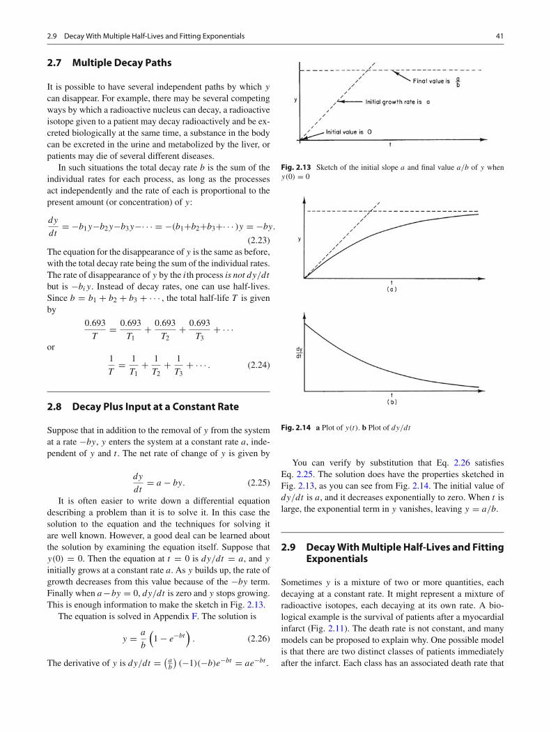
initially grows at a constant rate a. As y builds up, the rate ofgrowth decreases from this value because of the −by term.Finally when a−by = 0, dy/dt is zero and y stops growing.This is enough information to make the sketch in Fig. 2.13.

The equation is solved in Appendix F. The solution is

y = a

b

(1 − e−bt

). (2.26)

The derivative of y is dy/dt = ( ab

)(−1)(−b)e−bt = ae−bt .

Fig. 2.13 Sketch of the initial slope a and final value a/b of y wheny(0) = 0

Fig. 2.14 a Plot of y(t). b Plot of dy/dt

You can verify by substitution that Eq. 2.26 satisfiesEq. 2.25. The solution does have the properties sketched inFig. 2.13, as you can see from Fig. 2.14. The initial value ofdy/dt is a, and it decreases exponentially to zero. When t islarge, the exponential term in y vanishes, leaving y = a/b.

2.9 DecayWithMultiple Half-Lives and FittingExponentials

Sometimes y is a mixture of two or more quantities, eachdecaying at a constant rate. It might represent a mixture ofradioactive isotopes, each decaying at its own rate. A bio-logical example is the survival of patients after a myocardialinfarct (Fig. 2.11). The death rate is not constant, and manymodels can be proposed to explain why. One possible modelis that there are two distinct classes of patients immediatelyafter the infarct. Each class has an associated death rate that


101

2

3

4567

102

2

3

4567

103

2

3

4567

104

14121086420

t

A: y = A1e-b1t + A2e

-b2t

B: Estimate thatA2e

-b2t = 500e-0.131t

C: Typicalsubtractionof B from A:400-300 = 100

D: Estimate thatA1e

-b1t =1000e-0.576t

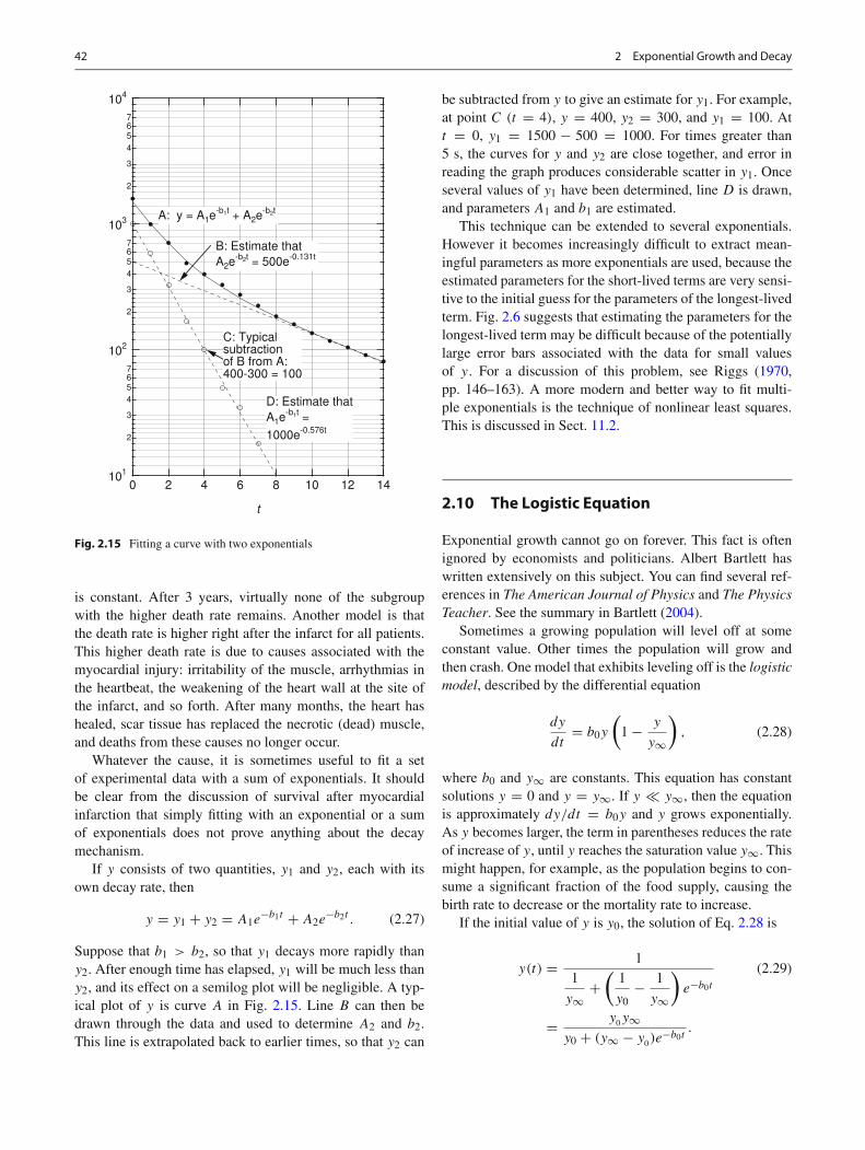
Fig. 2.15 Fitting a curve with two exponentials

is constant. After 3 years, virtually none of the subgroupwith the higher death rate remains. Another model is thatthe death rate is higher right after the infarct for all patients.This higher death rate is due to causes associated with themyocardial injury: irritability of the muscle, arrhythmias inthe heartbeat, the weakening of the heart wall at the site ofthe infarct, and so forth. After many months, the heart hashealed, scar tissue has replaced the necrotic (dead) muscle,and deaths from these causes no longer occur.

Whatever the cause, it is sometimes useful to fit a setof experimental data with a sum of exponentials. It shouldbe clear from the discussion of survival after myocardialinfarction that simply fitting with an exponential or a sumof exponentials does not prove anything about the decaymechanism.

If y consists of two quantities, y1 and y2, each with itsown decay rate, then

y = y1 + y2 = A1e−b1t + A2e

−b2t . (2.27)

Suppose that b1 > b2, so that y1 decays more rapidly thany2. After enough time has elapsed, y1 will be much less thany2, and its effect on a semilog plot will be negligible. A typ-ical plot of y is curve A in Fig. 2.15. Line B can then bedrawn through the data and used to determine A2 and b2.This line is extrapolated back to earlier times, so that y2 can

be subtracted from y to give an estimate for y1. For example,at point C (t = 4), y = 400, y2 = 300, and y1 = 100. Att = 0, y1 = 1500 − 500 = 1000. For times greater than5 s, the curves for y and y2 are close together, and error inreading the graph produces considerable scatter in y1. Onceseveral values of y1 have been determined, line D is drawn,and parameters A1 and b1 are estimated.

This technique can be extended to several exponentials.However it becomes increasingly difficult to extract mean-ingful parameters as more exponentials are used, because theestimated parameters for the short-lived terms are very sensi-tive to the initial guess for the parameters of the longest-livedterm. Fig. 2.6 suggests that estimating the parameters for thelongest-lived term may be difficult because of the potentiallylarge error bars associated with the data for small valuesof y. For a discussion of this problem, see Riggs (1970,pp. 146–163). A more modern and better way to fit multi-ple exponentials is the technique of nonlinear least squares.This is discussed in Sect. 11.2.

2.10 The Logistic Equation

Exponential growth cannot go on forever. This fact is oftenignored by economists and politicians. Albert Bartlett haswritten extensively on this subject. You can find several ref-erences in The American Journal of Physics and The PhysicsTeacher. See the summary in Bartlett (2004).

Sometimes a growing population will level off at someconstant value. Other times the population will grow andthen crash. One model that exhibits leveling off is the logisticmodel, described by the differential equation

dy

dt= b0y

(1 − y

y∞

), (2.28)

where b0 and y∞ are constants. This equation has constantsolutions y = 0 and y = y∞. If y y∞, then the equationis approximately dy/dt = b0y and y grows exponentially.As y becomes larger, the term in parentheses reduces the rateof increase of y, until y reaches the saturation value y∞. Thismight happen, for example, as the population begins to con-sume a significant fraction of the food supply, causing thebirth rate to decrease or the mortality rate to increase.

If the initial value of y is y0, the solution of Eq. 2.28 is

y(t) = 11

y∞+(

1

y0− 1

y∞

)e−b0t

(2.29)

= y0y∞y0 + (y∞ − y0)e

−b0t.

2.11 Log–log Plots, Power Laws, and Scaling 43

1.0

0.8

0.6

0.4

0.2

0.0

y

120100806040200

t

Exponential

Logistic

Fig. 2.16 Plot of the solution of the logistic equation when y0 = 0.1,y∞ = 1.0, b0 = 0.0667. Exponential growth with the same values ofy0 and b0 is also shown

You can easily verify that y(0) = y0 and y(∞) = y∞. A plotof the solution is given in Fig. 2.16, along with exponentialgrowth with the same value of b0.

Another way to think of Eq. 2.28 is that it has the formdy/dt = b(y)y, where b(y) = b0(1 − y/y∞) is now afunction of the dependent variable y instead of the indepen-dent variable t . As y grows toward the asymptotic value,the growth rate b(y) decreases linearly to zero. The logisticmodel was an early and very important model for popula-tion growth. It provides good fits in a few cases, but there arenow many more sophisticated models in population biology(Murray 2001) and bacterial growth (Hagen 2010).

2.11 Log–log Plots, Power Laws, and Scaling

This section considers the use of plots in which both scalesare logarithmic: log–log plots. They are useful when x and y

are related by the power law

y = Bxn. (2.30)

Notice the difference between this and the exponential func-tion: here the independent variable x is raised to a constantpower, while in the exponential case, x (or t) is in the expo-nent. It also leads to a discussion of scaling, whereby simplephysical arguments lead to important conclusions about thevariations between species in size, shape, metabolic rate, andthe like.

0.1

2

3

4567

1

2

3

4567

10

y

0.12 3 4 5 6 7

12 3 4 5 6 7

10

y = x1/2

y = x y = x2 y = x-1

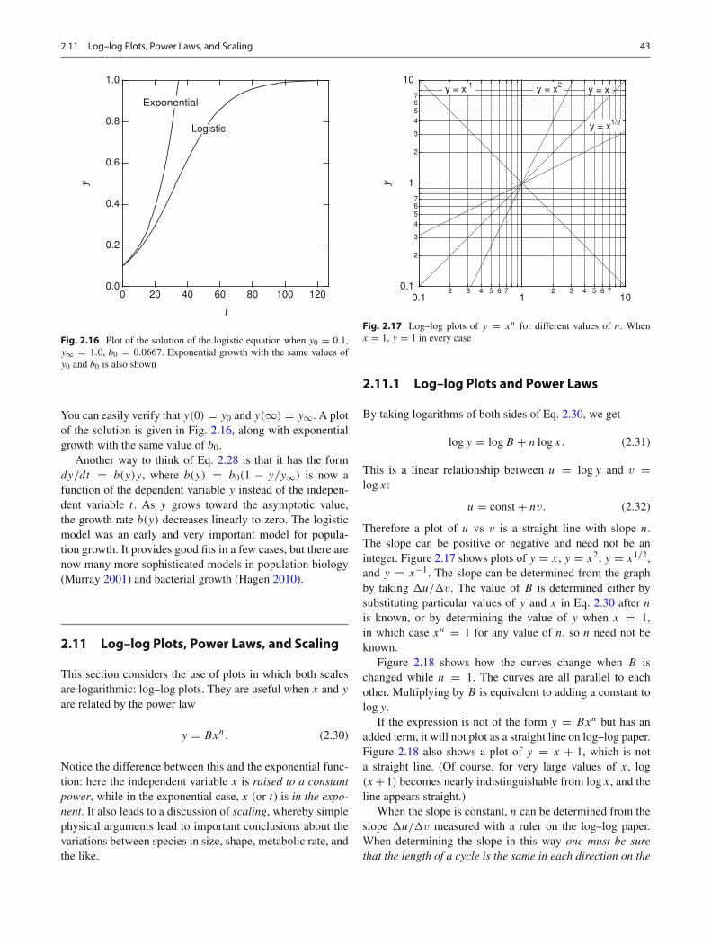
Fig. 2.17 Log–log plots of y = xn for different values of n. Whenx = 1, y = 1 in every case

2.11.1 Log–log Plots and Power Laws

By taking logarithms of both sides of Eq. 2.30, we get

log y = log B + n log x. (2.31)

This is a linear relationship between u = log y and v =log x:

u = const + nv. (2.32)

Therefore a plot of u vs v is a straight line with slope n.The slope can be positive or negative and need not be aninteger. Figure 2.17 shows plots of y = x, y = x2, y = x1/2,and y = x−1. The slope can be determined from the graphby taking �u/�v. The value of B is determined either bysubstituting particular values of y and x in Eq. 2.30 after n

is known, or by determining the value of y when x = 1,in which case xn = 1 for any value of n, so n need not beknown.

Figure 2.18 shows how the curves change when B ischanged while n = 1. The curves are all parallel to eachother. Multiplying by B is equivalent to adding a constant tolog y.

If the expression is not of the form y = Bxn but has anadded term, it will not plot as a straight line on log–log paper.Figure 2.18 also shows a plot of y = x + 1, which is nota straight line. (Of course, for very large values of x, log(x +1) becomes nearly indistinguishable from log x, and theline appears straight.)

When the slope is constant, n can be determined from theslope �u/�v measured with a ruler on the log–log paper.When determining the slope in this way one must be surethat the length of a cycle is the same in each direction on the


0.1

2

3

4567

1

2

3

4567

10y

0.12 3 4 5 6 7

12 3 4 5 6 7

10x

y = 0.5x

y = x

y = 4x

y = x + 1

Fig. 2.18 Log–log plots of y = Bx, showing how the curves shift onthe paper as B changes. Since n = 1 for all the curves, they all have thesame slope. There is also a plot of y = x + 1 to show that a polynomialdoes not plot as a straight line

graph paper. To repeat the warning: it is easy to get a roughidea of the exponent from inspection of the slope of the log–log plot in Fig. 2.17 because on commercial log–log graphpaper, the distance spanned by a decade or cycle is the sameon both axes. Some magazines routinely show log–log plotsin which the distance spanned by a decade is not the sameon both axes. Moreover, commercial graphing software doesnot impose this constraint on log–log plots, so it is becomingless and less likely that you can determine the exponent byglancing at the plot. Be careful!

When using a spreadsheet or other graphing software, itis often useful to make an extra column that contains the cal-culated variable ycalc = Axm with the values for A and m

stored in two cells of the spreadsheet. If you plot this columnas a line, and your real data as points without a line, then youcan change the parameters while inspecting the graph to findthe values that give the best fit.

An example of the use of a log–log plot is Poiseuille flowof fluid through a tube vs tube radius when the pressure gra-dient along the tube is constant (Problem 39). It was shownin Chap. 1 that an r4 dependence is expected.

2.11.2 Food Consumption, Basal MetabolicRate, and Scaling

Consider the relation of daily food consumption to bodymass. This will introduce us to simple scaling arguments.As a first model, we might suppose that each kilogram of

102

2

3

4567

103

2

3

4567

104

Ene

rgy

(kca

l/day

) or

Hei

ght (

mm

)

12 3 4 5 6 7

102 3 4 5 6 7

100Body Mass (kg)

Energy vs. Mass Height vs. Mass

Slope = 0.75

Slope = 0.62

Slope = 0.33

Fig. 2.19 Plot of daily food requirement F and height H vs mass M

for growing children. (Data are from Kempe et al. 1970, p. 90)

tissue has the same metabolic requirement, so that foodconsumption should be proportional to body mass. However,there is a problem with this argument. Most of the food thatwe consume is converted to heat. The various mechanismsto lose heat—radiation, convection, and perspiration—areall roughly proportional to the surface area of the bodyrather than its mass. (This statement neglects the fact thatconsiderable evaporation takes place through the lungsand that the body can control the rate of heat loss throughsweating and shivering.) If all persons were the same shape,then the total surface area would be proportional to H 2,where H is the height. The total volume and mass would beproportional to H 3, so H would be proportional to M1/3.Therefore the surface area would be proportional to (M1/3)2

or M2/3. (See Problem 44 for a discussion of other possibledependences of surface area on mass.) Figure 2.19 plots H

and the total daily food requirement F vs body mass M forgrowing children (Kempe et al. 1970, p. 90).

Neither of the models proposed above fits the data verywell. At early ages, H is more nearly proportional to M0.62

than to M1/3. For older children, when the shape of the bodyhas stopped changing, an M0.33 dependence does fit better.This better fit occurs for masses greater than 23 kg, whichcorrespond to ages over 6 years. The slope of the F(M)

curve is 0.75. This is less than the 1.0 of the model that foodconsumption is proportional to the mass and greater than the0.67 of the model that food consumption is proportional tosurface area.

This 34 -power dependence is remarkable because it is

seen across many species, from one-celled organisms to

Symbols Used 45

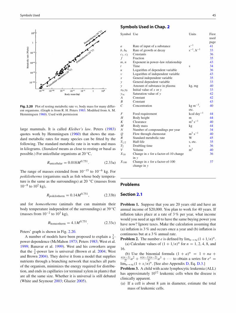
Fig. 2.20 Plot of resting metabolic rate vs. body mass for many differ-ent organisms. (Graph is from R. H. Peters 1983. Modified from A. M.Hemmingsen 1960). Used with permission

large mammals. It is called Kleiber’s law. Peters (1983)quotes work by Hemmingsen (1960) that shows the stan-dard metabolic rates for many species can be fitted by thefollowing. The standard metabolic rate is in watts and massin kilograms. (Standard means as close to resting or basal aspossible.) For unicellular organisms at 20 ◦C,

Runicellular = 0.018M0.751. (2.33a)

The range of masses extended from 10−15 to 10−6 kg. Forpoikilotherms (organisms such as fish whose body tempera-ture is the same as the surroundings) at 20 ◦C (masses from10−8 to 102 kg),

Rpoikilotherm = 0.14M0.751, (2.33b)

and for homeotherms (animals that can maintain theirbody temperature independent of the surroundings) at 39 ◦C(masses from 10−2 to 103 kg),

Rhomeotherm = 4.1M0.751. (2.33c)

Peters’ graph is shown in Fig. 2.20.A number of models have been proposed to explain a 3

4 -power dependence (McMahon 1973; Peters 1983; West et al.1999; Banavar et al. 1999). West and his coworkers arguethat the 3

4 -power law is universal (Brown et al. 2004; Westand Brown 2004). They derive it from a model that suppliesnutrients through a branching network that reaches all partsof the organism, minimizes the energy required for distribu-tion, and ends in capillaries (or terminal xylem in plants) thatare all the same size. Whether it is universal is still debated(White and Seymour 2003; Glazier 2005).

Symbols Used in Chap. 2Symbol Use Units First

usedpage

a Rate of input of a substance s−1 41b, b0 Rate of growth or decay s−1, h−1 33c1, c2 Constants 36f Fraction 35m, n Exponent in power–law relationship 43t Time s 34u Logarithm of dependent variable 36v Logarithm of independent variable 43x General independent variable 35y General dependent variable 33y Amount of substance in plasma kg, mg 40x0,y0 Initial value of x or y 33y∞ Saturation value of y 42A Constant 42B Constant 43C Concentration kg m−3,

etc.40

F Food requirement kcal day−1 44H Body height m 44K Clearance m3 s−1 40M Body mass kg 44N Number of compoundings per year 34Q Flow through chemostat m3 s−1 40R Standard metabolic rate W 45T1/2 Half-life s, etc. 35T2 Doubling time s 36V Volume m3 40X10 Change in x for a factor-of-10 change

in y

36

X100 Change in x for a factor-of-100change in y

37

Problems

Section 2.1

Problem 1. Suppose that you are 20 years old and have anannual income of $20,000. You plan to work for 40 years. Ifinflation takes place at a rate of 3 % per year, what incomewould you need at age 60 to have the same buying power youhave now? Ignore taxes. Make the calculation assuming that(a) inflation is 3 % and occurs once a year and (b) inflation iscontinuous but at a 3 % annual rate.Problem 2. The number e is defined by limn→∞(1+1/n)n.

(a) Calculate values of (1 + 1/n)n for n = 1, 2, 4, 8, and16.

(b) Use the binomial formula (1 + a)n = 1 + na +n(n−1)

2! a2 + n(n−1)(n−2)3! a3 + · · · to obtain a series for ex =

limn→∞(1 + x/n)n. [See also Appendix D, Eq. D.3.]Problem 3. A child with acute lymphocytic leukemia (ALL)has approximately 1012 leukemic cells when the disease isclinically apparent.(a) If a cell is about 8 μm in diameter, estimate the total

mass of leukemic cells.


(b) Cure requires killing every single cell. The doublingtime for the cells is about 5 days. If all cells were killedexcept for one, how long would it take for the disease tobecome apparent again?

(c) Suppose that chemotherapy reduces the number of cellsto 109 and there are no changes of ALL cell proper-ties (no mutations). How long a remission would youexpect? What if the number were reduced to 106?

Problem 4. Suppose that tumor cells within the body repro-duce at rate r , so that the number is given by y = y0e

rt . Eachtime a chemotherapeutic agent is given, it destroys a fractionf of the cells then existing. Make a semilog plot showing y

as a function of time for several administrations of the drug,separated by time T . What different cases must you considerfor the relation among f , T , and r?Problem 5. An exponentially growing culture of bacteria in-creases from 106 to 5 × 108 cells in 6 h. What is the timebetween successive cell divisions if there is no cell mortality?Problem 6. The following data on railroad tracks wereobtained from R. H. Romer (1991).

Year Miles of track1860 30,6261870 52,9221880 93,2621890 166,703

(a) What is the doubling time?(b) Estimate the surface area of the contiguous USA. As-

sume that a railroad roadbed is 7-m wide. In what yearwould an extrapolation predict that the surface of theUSA would be completely covered with railroad track?

Section 2.2

Problem 7. A dose D of drug is given that causes the plasmaconcentration to rise from 0 to C0. The concentration thenfalls according to C = C0e

−bt . At time T , what dose must begiven to raise the concentration to C0 again? What will hap-pen if the original dose is administered over and over againat intervals of T ?Problem 8. Consider the atmosphere to be at constant tem-perature but to have a pressure p that varies with heighty. A slab between y and y + dy has a different pressureon the top than on the bottom because of the weight ofthe air in the slab. (The weight of the air is the number ofmolecules N times mg, where m is the mass of a moleculeand g is the gravitational acceleration.) Use the ideal gas law,pV = NkBT (where kB is the Boltzmann constant and T ,the absolute temperature, is constant), and the fact that theair is in equilibrium to write a differential equation for p as

a function of y. The equation should be familiar. Show thatp(y) = Ce−mgy/kBT .Problem 9. The mean life of a radioactive substance isdefined by the equation

τ = − ∫∞0 t (dy/dt) dt

− ∫∞0 (dy/dt) dt

.

Show that if y = y0e−bt , then τ = 1/b.

Section 2.3

Problem 10. R. Guttman (1966) measured the temperaturedependence of the current pulse necessary to excite the squidaxon. She found that for pulses shorter than a certain lengthτ , a fixed amount of electric charge was necessary to makethe nerve fire; for longer pulses, the current was fixed. Thissuggests that the axon integrates the current for a time τ

but no longer. The following data are for the integratingtime τ vs temperature T (◦C). Find an empirical exponentialrelationship between T and τ .

T (◦C) τ (ms)5 4.110 3.415 1.920 1.425 0.730 0.635 0.4

Problem 11. A normal rabbit was injected with 1 cm3 ofStaphylococcus aureus culture containing 108 organisms. Atvarious later times, 0.2 cm3 of blood was taken from therabbit’s ear. The number of organisms per cm3 was calcu-lated by diluting the material, smearing it on culture plates,and counting the number of colonies formed. The results areshown below. Plot these data and see if they can be fit by asingle exponential. Can you also estimate the blood volumeof the rabbit?

t (min) Bacteria (cm−3)0 5 × 105

3 2 × 105

6 5 × 104

10 7 × 103

20 3 × 102

30 1.7 × 102

Section 2.4

Problem 12. All members of a certain population are bornat t = 0. The death rate in this population (deaths per unit

Problems 47

population per unit time) is found to increase linearly withage t : (death rate) = a+bt . Find the population as a functionof time if the initial population is y0.Problem 13. The accompanying table gives death rates (inyr−1) as a function of age. Plot these data on linear graphpaper and on semilog paper. Find a region over which thedeath rate rises approximately exponentially with age, anddetermine parameters to describe that region.

Age Death rate Age Death rate0 0.000 863 45 0.005 7765 0.000 421 50 0.008 986

10 0.000 147 55 0.013 74815 0.001 027 60 0.020 28120 0.001 341 65 0.030 70525 0.001 368 70 0.046 03130 0.001 697 75 0.066 19635 0.002 467 80 0.101 44340 0.003 702 85 0.194 197

Problem 14. Suppose that the amount of a resource at timet is y(t). At t = 0, the amount is y0. The rate at which itis consumed is r = −dy/dt . Let r = r0e

bt , that is, the rateof use increases exponentially with time. (For example, untilrecently the world use of crude oil had been increasing about7 % per year since 1890.)(a) Show that the amount remaining at time t is y(t) = y0 −

(r0/b)(ebt − 1).(b) If the present supply of the resource were used up at con-

stant rate r0, it would last for a time Tc. Show that whenthe rate of consumption grows exponentially at rate b,the resource lasts a time Tb = (1/b) ln(1 + bTc).

(c) An advertisement in Scientific American, September1978, p. 181, said, “There’s still twice as much gas un-derground as we’ve used in the past 50 years—at ourpresent rate of use, that’s enough to last about 60 years.”Calculate how long the gas would last if it were used ata rate that increases 7 % per year.

(d) If the supply of gas were doubled, how would the answerto part (c) change?

(e) Repeat parts (c) and (d) if the growth rate is 3 % per year.Problem 15. When we are dealing with death or compo-nent failure, we often write Eq. 2.17 in the form y(t) =y0 exp

[− ∫ t

0 m(t ′)dt ′]

and call m(t) the mortality function.

Various forms for the mortality function can represent fail-ure of computer components, batteries in pacemakers, orthe death of organisms. (This is not the most general possi-ble mortality model. For example, it ignores any interactionbetween organisms, so it cannot account for effects such asovercrowding or a limited supply of nutrients.)(a) For human populations, the mortality function is often

written as m(t) = m1e−b1t + m2 + m3e

+b3t . What sortof processes does each of these terms represent?

(b) Assume that m1 and m2 are zero. Then m(t) is called theGompertz mortality function. Obtain an expression fory(t) with the Gompertz mortality function. Time tmax

is sometimes defined to be the time when y(t) = 1. Itdepends on y0. Obtain an expression for tmax.

Problem 16. The incidence of a disease is the number ofnew cases per unit time per unit population (or per 100,000).The prevalence of the disease is the number of cases perunit population. For each situation below, the size of the gen-eral population remains fixed at the constant value y, and thedisease has been present for many years.(a) The incidence of the disease is a constant, i cases per

year. Each person has the disease for a fixed time ofT years, after which the person is either cured or dies.What is the prevalence p? Hint: the number who are sickat time t is the total number who became sick betweent − T and t .

(b) The patients in part (a) who are sick die with a constantdeath rate b. What is the prevalence?

(c) A new epidemic begins at t = 0, and the incidence in-creases exponentially with time: i = i0e

kt . What is theprevalence if each person has the disease for T years?

Section 2.5

Problem 17. The creatinine clearance test measures a pa-tient’s kidney function. Creatinine is produced by muscle ata rate p g h−1. The concentration in the blood is C g l−1. Thevolume of urine collected in time T (usually 24 h) is V l. Thecreatinine concentration in the urine is U g l−1. The clear-ance is K . The plasma volume is Vp. Assume that creatinineis stored only in the plasma.(a) Draw a block diagram for the process and write a

differential equation for C.(b) Find an expression for the creatinine clearance K in

terms of p and C when C is not changing with time.(c) If C is constant, all creatinine produced in time T ap-

pears in the urine. Find K in terms of C, V , U , andT .

(d) If p were somehow doubled, what would be the newsteady-state value of C? What would be the time con-stant for change to the new value?

Problem 18. A liquid is injected in muscle and spreadsthroughout a spherical volume V = 4πr3/3. The volumeis well supplied with blood, so that the liquid is removedat a rate proportional to the remaining mass per unit vol-ume. Let the mass be m and assume that r remains fixed.Find a differential equation for m(t) and show that m decaysexponentially.Problem 19. A liquid is injected as in Problem 18, but thistime a cyst is formed. The rate of removal of mass is pro-portional to both the pressure of liquid within the cyst, and


to the surface area of the cyst, which is 4πr2. Assume thatthe cyst shrinks so that the pressure of liquid within the cystremains constant. Find a differential equation for the rate ofmass removal and show that dm/dt is proportional to m2/3.Problem 20. The following data showing ethanol concen-tration in the blood vs time after ethanol ingestion are fromBennison and Li (1976, pp. 9–13). Plot the data and discussthe process by which alcohol is metabolized.

t (min) Ethanol concentration (mg dl−1)90 134

120 120150 106180 93210 79240 65270 50

Problem 21. Consider the following two-compartmentmodel. Compartment 1 is damaged myocardium (heart mus-cle). Compartment 2 is the blood of volume V . At t = 0,the patient has a heart attack and compartment 1 is created.It contains q molecules of some chemical that was releasedby the dead cells. Over the next several days, the chemi-cal moves from compartment 1 to compartment 2 at a ratei(t), such that q = ∫∞

0 i(t)dt . The amount of substance incompartment 2 is y(t) and the concentration is C(t). Theonly mode of removal from compartment 2 is clearance withclearance constant K .(a) Write a differential equation for C(t) that may also

involve i(t).(b) Integrate the equation and show that q can be determined

by numerical integration if C(t) and K are known.(c) Show that volume V need not be known if C(0) =

C(∞).

Section 2.7

Problem 22. The radioactive nucleus 64Cu decays indepen-dently by three different paths. The relative decay rates ofthese three modes are in the ratio 2:2:1. The half-life is12.8 h. Calculate the total decay rate b, and the three partialdecay rates b1, b2, and b3.Problem 23. The following data were taken from Berg et al.(1982). At t = 0, a 70-kg subject was given an intravenousinjection of 200 mg of phenobarbital. The initial concentra-tion in the blood was 6 mg l−1. The concentration decayedexponentially with a half-life of 110 h. The experiment wasrepeated, but this time the subject was fed 200 g of activatedcharcoal every 6 h. The concentration of phenobarbital againfell exponentially, but with a half-life of 45 h.(a) What was the volume in which the phenobarbital was

distributed?

(b) What was the clearance in the first experiment?(c) What was the clearance due to charcoal?

Section 2.8

Problem 24. You are treating a severely ill patient with anintravenous antibiotic. You give a loading dose D mg, whichdistributes immediately through blood volume V to give aconcentration C mg dl−1 (1 dl = 0.1 l). The half-life of thisantibiotic in the blood is T h. If you are giving an intravenousglucose solution at a rate R ml h−1, what concentration ofantibiotic should be in the glucose solution to maintain theconcentration in the blood at the desired value?Problem 25. The solution to the differential equationdy/dt = a − by for the initial condition y(0) = 0 isy = (a/b)(1 − e−bt ). Plot the solution for a = 5 g min−1

and for b = 0.1, 0.5, and 1.0 min−1. Discuss why the finalvalue and the time to reach the final value change as they do.Also make a plot for b = 0.1 and a = 10 to see how thatchanges the situation.Problem 26. Derive an approximate expression for(a/b)

(1 − e−bt

)which is accurate for small times (t

1/b). Use the Taylor expansion for an exponential given inAppendix D.Problem 27. We can model the repayment of a mortgagewith a differential equation. Suppose that y(t) is the amountstill owed on the mortgage at time t , the rate of repaymentper unit time is a, b is the interest rate, and the initial amountof the mortgage is y0.(a) Find the differential equation for y(t).(b) Try a solution of the form y(t) = a/b + Cebt , where

C is a constant to be determined from the initial condi-tions. Find C, plot the solution, and determine the timerequired to pay off the mortgage.

Problem 28. When an animal of mass m falls in air, twoforces act on it: gravity, mg, and a force due to air friction.Assume that the frictional force is proportional to the speedv.(a) Write a differential equation for v based on Newton’s

second law, F = m(dv/dt).(b) Solve this differential equation (hint: compare your

equation to Eq. 2.25).(c) Assume that the animal is spherical, with radius a and

density ρ. Also, assume that the frictional force is pro-portional to the surface area of the animal. Determinethe terminal speed (speed of descent in steady state) asa function of a.

(d) Use your result in part (c) to interpret the followingquote by J. B. S. Haldane (1985): “You can drop amouse down a thousand-yard mine shaft; and arrivingat the bottom, it gets a slight shock and walks away. Arat is killed, a man is broken, a horse splashes.”

Problems 49

Problem 29. In Problem 28, we assumed that the force ofair friction is proportional to the speed v. For flow at highReynolds numbers, a better approximation is that the force is−kv2.(a) Write the differential equation for v as a function of t .(b) This differential equation is nonlinear because of the v2

term and thus difficult to solve analytically. However,the terminal speed can easily be obtained directly fromthe differential equation by setting dv/dt = 0. Find theterminal speed as a function of a (defined in Problem28).

(c) Verify that v(t) = √mg/k tanh

(√kg/mt

)is a solution.

Problem 30. A drug is infused into the body through an in-travenous drip at a rate of 100 mg h−1. The total amount ofdrug in the body is y. The drug distributes uniformly andinstantaneously throughout the body in a compartment ofvolume V = 18 l. It is cleared from the body by a singleexponential process. In the steady state, the total amount inthe body is 200 mg.(a) At noon (t = 0), the intravenous line is removed. What

is y(t) for t > 0?(b) What is the clearance of the drug?

Section 2.9

Problem 31. You are given the following data:

x y x y

0 1.000 5 0.4441 0.800 6 0.4002 0.667 7 0.3643 0.571 8 0.3334 0.500 9 0.308

10 0.286

Plot these data on semilog graph paper. Is this a single expo-nential? Is it two exponentials? Plot 1/y vs x. Does this alteryour answer?Problem 32. Cells can repair DNA damage caused by x-rayexposure (see Sect. 16.9). Wang et al. (2001) found that theamount of damage is characterized by two time constants.Assume the DNA damage, D, as a function of time, t , isgiven by the following data

t (h) D(%) t (h) D(%)0 100 1.5 160.25 46 2 140.50 28 4 9.00.75 21 6 5.81.0 18 8 3.7

Plot the data on semilog paper. Fit the data to Eq. 2.27 byeye or using a spreadsheet and determine A1, A2, b1, and b2.

Note that the data are normalized to 100 % at t = 0. Whatdoes this mean in terms of A1 and A2?

Section 2.10

Problem 33. Suppose that the rate of consumption of a re-source increases exponentially. (This might be petroleum, orthe nutrient in a bacterial culture.) During the first doublingtime, the amount used is 1 unit. During the second doublingtime, it is 2 units, the next 4, etc. How does the amount con-sumed during a doubling time compare to the total amountconsumed during all previous doubling times?Problem 34. Suppose that the rate of growth of y is de-scribed by dy/dt = b(y)y. Expand b(y) in a Taylor’sseries and relate the coefficients to the terms in the logisticequation.Problem 35. Verify that the solution y(t) in Eq. 2.29 obeysthe differential Eq. 2.28.Problem 36. In the logistic model (Eq. 2.28), what value ofy corresponds to the maximum rate of change of y?Problem 37. The consumption of a finite resource isoften modeled using the logistic equation. Let y(t) be thecumulative amount of a resource consumed and y∞ bethe total amount that was initially available at t = −∞.

Model the rate of consumption using Eq. 2.29 over the range−∞ < t < ∞.(a) Set y0 = y∞/2, so that the zero of the time axis

correponds to when half the resource has been used.Show that this simplifies Eq. 2.29.

(b) Differentiate y(t) to find an expression for the rateof consumption. Sketch plots of dy/dt vs t on linearand semilog graph paper. When does the peak rate ofconsumption occur?

When this model is applied to world oil consumption, themaximum is called Hubbert’s peak (Deffeyes 2008).Problem 38. Consider a classic predator–prey problem. Letthe number of foxes be F and the number of rabbits be R.The rabbits eat grass, which is plentiful. The foxes eat onlyrabbits. The number of foxes and rabbits can be modeled bythe Lotka–Volterra equations

dR

dt= aR − bRF

dF

dt= −cF + dRF.

(a) Describe the physical meaning of each term on the right-hand side of each equation. What does each of theconstants a, b, c, and d denote?

(b) Solve for the steady-state values of F and R.These differential equations are difficult to solve because

they are nonlinear (see Chap. 10). Typically, R and F oscil-late about the steady-state solutions found in (b). For moreinformation, see Murray (2001).


Section 2.11

Problem 39. Plot the following data for Poiseuille flow onlog–log graph paper. Fit the equation i = CRn

p to the data byeye (or by trial and error using a spread sheet), and determineC and n.

Rp(μm) i(μm3s−1)

5 0.000 107 0.000 3810 0.001 615 0.008 120 0.02630 0.1350 1.0

Problem 40. Below are the molecular weights and radiiof some molecules. Use log–log graph paper to develop anempirical relationship between them.

Substance M R (nm)Water 18 0.15Oxygen 32 0.20Glucose 180 0.39Mannitol 180 0.36Sucrose 390 0.48Raffinose 580 0.56Inulin 5 000 1.25Ribonuclease 13,500 1.8β-lactoglobin 35,000 2.7Hemoglobin 68,000 3.1Albumin 68,000 3.7Catalase 250,000 5.2

Problem 41. How well does Eq. 2.33c explain the data ofFig. 2.19? Discuss any differences.Problem 42. Compare the mass and metabolic requirements(and hence waste output, including water vapor) of 180 peo-ple each weighing 70 kg with 12,600 chickens of averagemass 1 kg.Problem 43. Figure 2.19 shows that in young children,height is more nearly proportional to M0.62 than to M1/3.Find pictures of children and adults and compare ratios ofheight to width, to see what the differences are.Problem 44. Consider three models of an organism. The firstis a sphere of radius R. The second is a cube of length L.These are crude models for animals. The third is a broad leafof surface area A on each side and thickness t . Assume allhave density ρ. In each case, calculate the surface area S asa function of mass, M . Ignore the surface area of the edge ofthe leaf. (For a comparison of scaling in leaves and animals,see Reich (2001). He shows that for broad leaves, S ∝ M1.1.)Problem 45. If food consumption is proportional to M3/4

across species, how does the food consumption per unit

mass scale with mass? Qualitatively compare the eatinghabits of hummingbirds to eagles and mice to elephants. (SeeSchmidt-Nielsen 1984, pp. 62–64.)Problem 46. In Problem 45, you found how the specificmetabolic rate (food consumption per unit mass) varies withmass. If all animal heart volumes and blood volumes are pro-portional to M , then the only way for the heart to increase theoxygen delivery to the body is by increasing the frequency ofthe heart rate (Schmidt-Nielsen 1984, pp. 126–150).(a) Using the result from Problem 45, if a 70 kg man has a

heart rate of 80 beats min−1, determine the heart rate ofa guinea pig (M = 0.5 kg).

(b) To a first approximation, all hearts beat about800,000,000 times in a lifetime. A 30-g mouse livesabout 3 years. Estimate the life span of a 3000-kgelephant.

(c) Humans live longer than what their mass would indi-cate. Calculate the life span of a 70-kg human based onscaling, and compare it to a typical human life span.

Problem 47. Let us examine how high animals can jump(Schmidt-Nielsen 1984, pp. 176–179). Assume that the en-ergy output of the jumping muscle is proportional to the bodymass, M . The gravitational potential energy gained uponjumping to a height h is Mgh (g = 9.8 m s−2). If a 3-g lo-cust can jump 60 cm, how high can a 70-kg human jump?Use scaling arguments.Problem 48. In Problem 47, you should have found that allanimals can jump to about the same height (approximately0.6 m), independent of their mass M .(a) Equate the kinetic energy at the bottom of the jump

(Mv2/2, where v is the“take-off speed”) to the poten-tial energy Mgh at the top of the jump to find how thetake-off speed scales with mass.

(b) Calculate the take-off speed.(c) In order to reach this speed, the animal must accelerate

upward over a distance L. If we assume a constant ac-celeration a, then a = v2/(2L). Assume L scales as thelinear size of the animal (and assume all animals are ba-sically the same shape but different size). How does theacceleration scale with mass?

(d) For a 70-kg human, L is about 1/3 m. Calculate theacceleration (express your answer in terms of g).

(e) Use your result from part (c) to estimate the accelerationfor a 0.5-mg flea (again, express your answer in terms ofg).

(f) Speculate on the biological significance of the result inpart (e) (See Schmidt-Nielsen 1984, pp. 180–181).

References 51

References

Banavar JR, Maritan A, Rinaldo A (1999) Size and form in efficienttransportation networks. Nature 399:130–132

Bartlett A (2004) The essential exponential! For the future of our planet.Center for Science, Mathematics & Computer Education, Lincoln

Bennison LJ, Li TK (1976) Alcohol metabolism in American Indiansand whites—lack of racial differences in metabolic rate and liveralcohol dehydrogenase. N Engl J Med 294:9–13

Berg MJ, Berlinger WG, Goldberg MJ, Spector R, Johnson GF (1982)Acceleration of the body clearance of phenobarbital by oral acti-vated charcoal. N Engl J Med 307:642–644

Bland EF, White PD (1941) Coronary thrombosis (with myocardialinfarction) ten years later. J Am Med Assoc 114(7):1171–1173

Brown JH, Gillooly JF, Allen AP, Savage VM, West GB (2004) Towarda metabolic theory of ecology. Ecology 85:1771–1789

Clark VA (1975) Survival distributions. Ann Rev Biophys Bioeng4:431–438

Deffeyes KS (2008) Hubbert’s peak: the impending world oil shortage.Princeton University Press, Princeton

Glazier DS (2005) Beyond the ‘3/4-power law’: Variation in the intra-and interspecific scaling of metabolic rate in animals. Biol Rev80:611–662

Guttman R (1966) Temperature characteristics of excitation inspace-clamped squid axons. J Gen Physiol 49:1007–1018.doi:10.1085/jgp.49.5.1007

Hagen SJ (2010) Exponential growth of bacteria: constant multiplica-tion through division. Am J Phys 78(12):1290–1296

Haldane JBS (1985) On being the right size and other essays. OxfordUniversity Press, Oxford

Hemmingsen AM (1960) Energy metabolism as related to body sizeand respiratory surfaces, and its evolution. Rep Steno Meml HospNordisk Insul Lab 9:6–110

Kempe CH, Silver HK, O’Brien D (1970) Current pediatric diagnosisand treatment, 2nd edn. Lange, Los Altos

Levy D, Brink S (2005) A change of heart: how the people of Framing-ham, Massachusetts helped unravel the mysteries of cardiovasculardisease. Knopf, New York

Maor E (1994) e, The story of a number. Princeton University Press,Princeton

McKee PA, Castelli WP, McNamara PM, Kannel WB (1971) The nat-ural history of congestive heart failure: the Framingham study. NEngl J Med 285:1441–1446

McMahon T (1973) Size and shape in biology. Science 179:1201–1204Murray JD (2001) Mathematical biology. Springer, New YorkPeters RH (1983) The ecological implications of body size. Cambridge

University Press, CambridgeReich P (2001) Body size, geometry, longevity and metabolism:

do plant leaves behave like animal bodies? Trends Ecol Evol16(12):674–680

Romer RH (1991) The mathematics of exponential growth—keep itsimple. Phys Teach 9:344–345

Riggs DS (1970) The mathematical approach to physiological prob-lems. MIT Press, Cambridge

Schmidt-Nielsen K (1984) Scaling: why is animal size so important?Cambridge University Press, Cambridge

Wang H, Zeng Z-C, Bui T-A, Sonoda E, Takata M, Takeda S, Iliakis G(2001) Efficient rejoining of radiation-induced DNA double-strandbreaks in vertebrate cells deficient of genes of the RAD52 epistasisgroup. Oncogene 20:2212–2224

West GB, Brown JH, Enquist BJ (1999) The fourth dimension oflife: fractal geometry and allometric scaling of organisms. Science284:1677–1679. (see also Mackenzie’s accompanying editorial onpage 1607 of the same issue of Science)

West GB, Brown JH (2004). Life’s universal scaling laws. Phys Today57(9):36–42

White CR, Seymour RS (2003) Mammalian basal metabolic rate is pro-portional to body mass2/3. Proc Natl Acad Sci U S A 100(7):4046–4049

Zumoff B, Hart H, Hellman L (1966) Considerations of mortality incertain chronic diseases. Ann Intern Med 64:595–601

exponential growth and decay

Documents