linear time byzantine self-stabilizing clock synchronization

Linear Time Byzantine Self-Stabilizing ClockSynchronization

Ariel Daliot1, Danny Dolev1?, and Hanna Parnas2

1 School of Engineering and Computer Science, The Hebrew University of Jerusalem,Israel. {adaliot,dolev}@cs.huji.ac.il

2 Department of Neurobiology and the Otto Loewi Minerva Center for Cellular andMolecular Neurobiology, Institute of Life Science, The Hebrew University of

Jerusalem, Israel. [email protected]

Abstract. Awareness of the need for robustness in distributed systemsincreases as distributed systems become an integral part of day-to-daysystems. Tolerating Byzantine faults and possessing self-stabilizing fea-tures are sensible and important requirements of distributed systems ingeneral, and of a fundamental task such as clock synchronization in par-ticular. There are efficient solutions for Byzantine non-stabilizing clocksynchronization as well as for non-Byzantine self-stabilizing clock syn-chronization. In contrast, current Byzantine self-stabilizing clock syn-chronization algorithms have exponential convergence time and are thusimpractical. We present a linear time Byzantine self-stabilizing clock syn-chronization algorithm, which thus makes this task feasible. Our deter-ministic clock synchronization algorithm is based on the observation thatall clock synchronization algorithms require events for re-synchronizingthe clock values. These events usually need to happen synchronously atthe different nodes. In these solutions this is fulfilled or aided by havingthe clocks initially close to each other and thus the actual clock valuescan be used for synchronizing the events. This implies that the clock val-ues cannot differ arbitrarily, which necessarily renders these solutions tobe non-stabilizing. Our scheme suggests using a tight pulse synchroniza-tion that is uncorrelated to the actual clock values. The synchronizedpulses are used as the events for re-synchronizing the clock values.

1 Introduction

Overcoming failures that are not predictable in advance is most suitably ad-dressed by tolerating Byzantine faults. It is the preferred fault model in orderto seal off unexpected behavior within limitations on the number of concur-rent faults. Most distributed tasks require the number of Byzantine faults, f , toabide by the ratio of 3f < n, where n is the network size. See [?] for impossibil-ity results on several consensus related problems such as clock synchronization.Additionally, it makes sense to require such systems to resume operation af-ter serious unpredictable events without the need for an outside interventionor restart of the system from scratch. E.g. systems may occasionally experience? This research was supported in part by Intel COMM Grant - Internet Net-

work/Transport Layer & QoS Environment (IXA)

2 Daliot, Dolev and Parnas

short periods in which more than a third of the nodes are faulty or messages sentby all nodes may be lost for some time. Such transient violations of the basicfault assumptions may leave the system in an arbitrary state from which theprotocol is required to resume in realizing its task. Typically, Byzantine algo-rithms do not ensure convergence in such cases. Byzantine algorithms focus onmerely preventing Byzantine faults from notably shifting the system state awayfrom the goal. They sometimes make strong assumptions on the initial state. Aself-stabilizing algorithm overcomes this limitation by converging within finitetime to a correct state from any initial state. Thus, even if the system loses itsconsistency due to a transient violation of the basic fault assumptions (e.g. morethan a third of the nodes being faulty, network disconnected, etc.) then once thesystem is back within the assumption boundaries the protocol will successfullyrealize the task, irrespective of the resumed state of the system. For a shortsurvey of self-stabilization see [?] and for an extensive study see [?].

The current paper addresses the problem of synchronizing clocks in a dis-tributed system. There are several efficient algorithms for self-stabilizing clocksynchronization withstanding crash faults (see [?,?,?] or other variants of theproblem [?,?]). There are many efficient classic Byzantine clock synchronizationalgorithms (for a performance evaluation of clock synchronization algorithmssee [?]), however strong assumptions on the initial state of the nodes are typicallymade, such as assuming all clocks are initially synchronized ([?,?,?]) and thusare not self-stabilizing. On the other hand, self-stabilizing clock synchronizationalgorithms can initiate with arbitrary values which can have a cost in the conver-gence times or in the severity of the faults contained. There are surprisingly fewself-stabilizing solutions facing Byzantine faults ([?]), which additionally haveunpractical convergence times. Note that self-stabilizing clock synchronizationhas an inherent difficulty in estimating real-time without an external time ref-erence due to the fact that non-faulty nodes may initialize with arbitrary clockvalues. Thus self-stabilizing clock synchronization aims at reaching a stable statefrom which clocks proceed synchronously at the rate of real-time and not nec-essarily estimate real-time (assuming that nodes have access to physical timersthat proceed close to real-time rate). Many applications utilizing the synchro-nization of clocks do not really require the exact real-time notion (see [?]). Insuch applications, agreeing on a common clock reading is sufficient as long asthe clocks progress within a linear envelope of any real-time interval.

We present a protocol with the following property: should the system beinitialized with clocks that hold values that are close to real-time then the clocksstay synchronized while attaining similar real-time accuracy, precision and timecomplexity as non-stabilizing clock synchronization protocols. Should the systeminitialize with arbitrary clock values or recover from any transient faults then theclocks synchronize very fast and proceed at real-time rate with high precision.

The protocol we present significantly improves upon existing Byzantine self-stabilizing clock synchronization algorithms by reducing the time complexityfrom expected exponential ([?]) to deterministic O(f). The comparably low com-plexity is achieved by focusing on a deterministic Byzantine self-stabilizing al-gorithm for pulse synchronization. The synchronized pulses progress at a pacethat allows the execution of a Byzantine Strong Consensus protocol on the clockvalues in between pulses, thus obtaining a common clock reading.

Byzantine Self-Stabilizing Clock Synchronization 3

A special challenge in self-stabilizing clock synchronization is the clock wraparound. In non-stabilizing algorithms having a large enough integer eliminatesthe problem for any practical concern. In self-stabilizing schemes a transientfailure can cause nodes to initialize with arbitrarily large clocks, surfacing theissue of the clock bounds. The clock synchronization schemes described abovehandles this wrap around.

Having access to an outside source of real-time is useful, though it introducesa single point of failure. Our approach is useful in such a case to overcome periodsin which the outside source fails in order to maintain a consistent system state.

2 Model and Problem Definition

The environment is a network of processors (nodes) that communicate by ex-changing messages. Individual nodes have no access to a central clock and thereis no global pulse system. The hardware clocks (referred to as the physical timers)of correct nodes have a bounded drift rate, ρ, from real-time. The communicationnetwork does not guarantee any order on messages.

The network and/or all the nodes can behave arbitrarily, though eventuallythe network performs within the defined assumption boundaries in which at mostf out of the n nodes may behave arbitrarily.Definition 1. The network assumption boundaries are:1. Message passing allowing for an authenticated identity of the senders.2. At most f of the nodes are faulty.3. Any message sent by any non-faulty node will eventually reach every non-

faulty node within δ time units.

Definition 2. A node is correct at times that it complies with the followingconditions:1. Obeys a global constant 0 < ρglob << 1, such that for every Newtonian time

interval [u, v], (1−ρglob)(v−u) ≤ ‘physical timer’(v)− ‘physical timer’(u) ≤(1 + ρglob)(v − u). Hereafter ρglob is denoted by ρ (typically ρ ≈ 10−6).

2. Operates according to the instructed protocol.

A node is considered faulty if it violates one or more of the above. A faultynode recovers from its faulty behavior if it resumes obeying the conditions of acorrect node. For consistency reasons the recovery is not immediate, but rathertakes a certain amount of time during which the node is still considered faultyalthough it behaves correctly3.

Basic notations:We use the following notations to define the quality of the solution, though nodesdo not need to maintain all of them as variables.– Clocki (the clock of node i) is a function of node pi’s physical timer that

returns a value in the range 0 to M − 1. Thus M − 1 is the maximal value aclock can hold. The clock is incremented every time unit. Clocki(t) denotesthe value of the clock of node pi at real-time t.

3 For example, a node may recover during the Byzantine Consensus procedure andviolate the validity condition if considered correct immediately.


– A “pulse” is an internal event for the re-synchronization of the clocks, ideallyevery cycle time units. A cycle is the time interval between two successivepulses that a node invokes.

– σ represents the upper bound on the real-time between the invocations ofthe pulses of different correct nodes (tightness of pulse synchronization).

– γ is the target upper bound on the difference of clock readings of any twocorrect clocks at any real-time. Our protocol achieves γ = 5d+c ·ρ, for someconstant c.

– Let a, b, g, h ∈ R+ be constants that define the linear envelope bound of theclock progression rate on any real-time interval.

– Ψi(t1, t2) is the amount of clock time elapsed on the clock of node pi during areal-time interval [t1, t2] within which pi was continuously correct. The valueof Ψ is not affected by any wrap around of clocki during that period.

– d ≡ δ + π, where π is the upper bound on message processing time.

Thus, d is an upper bound on the elapsed real-time from sending a messageby a non-faulty node until it is received and processed by every non-faulty node.

Using the above notations, a recovered node can be considered correct once itgoes through a complete synchronization process, which is guaranteed to happenwithin cycle+ BYZ_time of correct behavior, where BYZ_time is the time tocomplete the Byzantine Consensus algorithm.

Definition 3. Clock_state

– The clock_state of the system at real-time t is given by:clock_state(t) ≡ (clock0(t), . . . , clockn−1(t)).

– The systems is in a synchronized clock_state at real-time t if∀correct pi, pj , |clocki(t)−clockj(t)| ≤ γ or4 |clocki(t)−clockj(t)| ≥M−γ.

Definition 4. The Self-Stabilizing Clock Synchronization ProblemAs long as the system is within the assumption boundaries:

Convergence: Starting from an arbitrary state, s, the system reaches a syn-chronized clock_state after a finite time.

Closure: If s is a synchronized clock_state of the system at real-time t0 then∀real time t ≥ t0,1. clock_state(t) is a synchronized clock_state,2. “Linear Envelope”: for every correct node, pi,

a · [t− t0] + b ≤ Ψi(t0, t) ≤ g · [t− t0] + h.

3 Self-Stabilizing Byzantine Clock Synchronization

A major challenge of self-stabilizing clock synchronization is to ensure clock syn-chronization even when nodes may initialize with arbitrary clock values. This,as mentioned before, requires handling the wrap around of clock values. The

4 The second condition is a result of dealing with bounded clock variables.


algorithm we present employs as a building block an underlying Byzantine self-stabilizing pulse synchronization procedure. In the pulse synchronization prob-lem nodes invoke pulses regularly, ideally every cycle time units, and the goal isto do so in tight synchrony. To synchronize their clocks, nodes initiate at everypulse a Strong Byzantine Consensus to agree on the clock value to be associatedwith the time of the next pulse event5. Once pulses are synchronized, then theconsensus results in synchronized clocks. The basic algorithm uses strong con-sensus to ensure that once correct clocks are synchronized at a certain pulse andthus enter the consensus procedure with identical values, then they terminatewith the same identical values and thus keep the progression of clocks continuousand synchronized6.

3.1 The Basic Algorithm

The basic algorithm is essentially a self-stabilizing version of the Byzantine clocksynchronization algorithm in [?]. We call it Pulse-Clock-Synch. The agreed clocktime of the next synchronization is denoted by ET (short for Expected Time, asin [?]). Synchronization of clocks is targeted to happen every cycle time units,unless the pulse is invoked earlier7.

Pulse-Clock-Synchat “pulse” event

beginClock = ET ;Abort possible running instance of Pulse-Clock-Synch and reset all buffers;Wait σ(1 + 2ρ) time units;Next_ET = Strong-Byz-Consensus((ET + cycle) mod M);Clock = (Clock +Next_ET − (ET + cycle)) mod M ;ET = Next_ET ;

end

The internal pulse event is delivered by the pulse synchronization procedure.This event stops all on-going agreements and previous invocations of Pulse-Clock-Synch and resets all buffers. The pulse synchronization procedure ensuresthat once pulses are synchronized, the Pulse-Clock-Synch are invoked within σreal-time units8 of the pulse invocations at all correct nodes.

The “Wait” intends to make sure that all correct nodes enter the ByzantineConsensus after the invocation of the pulse event at all correct nodes, withoutremnants of past invocations. Existence of past remnants may happen only whenthe system is not yet synchronized or it is not within the assumption boundaries.

A correct node joins a Byzantine Consensus only concomitant to an inter-nal pulse event, as instructed by the Pulse-Clock-Synch. The Strong-Byzantine-5 It is assumed that the time between successive pulses is sufficient for a Byzantine

Consensus algorithm to initiate and terminate in between.6 The Pulse Synchronization building block does not use the value of the clock to

determine its progress, but rather intervals measured on the physical timer.7 cycle has the same function as PER in [?].8 The pulse synchronization presented achieves σ = 2d.


Consensus is intended to reach consensus on the next value of ET. One canuse a synchronous agreement algorithm with rounds of size (σ + d)(1 + 2ρ) orasynchronous style agreement in which a node waits to get n − f messages ofthe previous round before moving to the next round. We assume the use of aByzantine Consensus algorithm tolerating f faults when n ≥ 3f + 1.

The Strong-Byzantine-Consensus also ensures that when the clocks are syn-chronized the wrap around of clocks happens at all correct nodes within a shorttime and at the same cycle.

The posterior clock adjustment (following the consensus) adds to the clockvalue the elapsed time since the pulse and until the end of the consensus, asif the time at the pulse was in accordance with the relevant time reflected bythe consensus for the next pulse. This intends to expedite the time for reachingsynchronized clocks in the case in which the node’s initial value of ET did notagree with the value at the rest of the correct nodes.

Notice that when the system is back within the assumption boundaries, fol-lowing a chaotic state, pulses may arrive to different nodes at arbitrary times, andnodes’ ET and clocks may differ arbitrarily. At that time not all nodes will jointhe Byzantine Consensus and no consistent resultant value can be guaranteed.Once the pulses become synchronized (guaranteed by the pulse synchronizationprocedure to happen within a single cycle) all correct nodes will join the sameexecution of the Byzantine Consensus and will agree on the clock value of thenext synchronization. From that time on, as long as the system stays within theassumption boundaries the clocks remain synchronized, similar to [?].

Note that instead of simply setting the clock value to ET we could use someClock-Adjust procedure (cf. [?]), which receives a parameter indicating the targetvalue of the clock. The procedure runs in the background, it speeds up or slowsdown the clock rate to reach the adjusted value within a specified period of time.The procedure handles clock wrap around.

Theorem 1. Pulse-Clock-Synch solves the Self-Stabilizing Clock Synchroniza-tion Problem in the presence of at most f Byzantine nodes, where n ≥ 3f + 1.

Proof. Assume that the Pulse Synchronization procedure that invokes the pulsessolves the Self-Stabilizing Pulse Synchronization Problem, as defined in Sec-tion ??, in the presence of at most f Byzantine nodes, where n ≥ 3f + 1.Assume that cyclemin ≥ 2σ + byz_time, where byz_time is the maximal timeit takes to complete the consensus algorithm.Convergence: Let the system be within the assumption boundaries, in an arbi-trary state, s, with the nodes holding arbitrary clock values. The pulse synchro-nization procedure is self-stabilizing, thus, independent of the system’s initialstate, within a finite time the pulses are invoked regularly and synchronouslywith a tightness of σ. At every pulse all remnants of previously invoked con-sensus algorithms are flushed by all the correct nodes. A correct node does notinitiate or join the consensus algorithm before waiting σ(1+2ρ) time units, hencenot before all correct nodes have invoked a pulse and subsequently flushed theirbuffers. All correct nodes will join the consensus, thus the consensus algorithmwill initiate and terminate successfully.

At termination of the first instance of the consensus algorithm following thesynchronization of the pulses, all correct nodes agree on the clock value to be


held at the next pulse invocation. Subsequently, all correct nodes adjust theirclocks, post factum, according to the agreed ET. Note that this posterior adjust-ment of the clocks does not affect the time span until the invocation of the nextpulse but rather updates the clocks concomitantly to and in accordance withthe newly agreed ET. This has an effect if the correct nodes entered the consen-sus with differing values. Hence if all correct nodes enter the consensus with thesame ET then the adjustment equals zero. Since all correct pulses arrived withinσ of each other, after the posterior clock adjustment of the last correct node, allcorrect clocks are within γ1 = σ(1 + 2ρ) + byz_end · 2ρ,9 where byz_end is themaximal span of time from the first pulse until the last correct node completesthe posterior clock adjustment. Correct clocks will continue to drift apart at arate of 2ρ until the next clock adjustment, which will take place in about a cycletime. The precision of the clocks (the bound on the clock differences), γ ≥ γ1,equals the bound on the precision of the pulse arrival and the accumulated skewon the upper bound cycle length. This concludes the Convergence condition.

Closure: Let the system be in a synchronized clock_state. Consider first thecase in which all correct nodes hold the same value for ET. In this case, eachcorrect node resets its clock when the pulse arrives and doesn’t adjust its clockafter the consensus, since the consensus value will be the same as the value itentered the consensus with. To simplify the discussion assume that no wraparound of any correct clock takes place during the time that the pulse arrives atthe first correct node and until it is invoked at the last correct node. Right afterthe pulse is invoked at the last correct node and it’s subsequent clock adjustment,all correct clocks are within γ0 = σ(1 + 2ρ) of each other.

From that point on clocks of correct nodes drift apart at a rate of 2ρ of eachother. As long as no wrap around of the clocks takes place and no pulse arrivesat any correct node, the clocks are at most γ0 +∆T · 2ρ apart, where ∆T is thereal-time elapsed since the invocation of the pulse at the first correct node. Theforth-coming pulses will be invoked at all correct nodes within at most cycle+σtime, thus the bound on the clock difference of correct nodes, before the firstpulse is invoked again is γ0 + cycle · 2ρ.

When a correct node resets its clock once a pulse arrives, the maximal clockadjustment is the maximal difference between its current clock value and thevalue of ET.We discuss this difference, denoted by ADJ, later on in the proof andin Section ??. The clocks will continue to drift apart until the last correct nodereceives its “pulse" event. Therefore, the maximal clock difference, as long as noclock wrap around takes place is bounded by ADJ+γ0+cycle·2ρ+σ(1+2ρ)2ρ ≤γ.

We now consider the case that a clock wrap around takes place at some ∆Ttime after the pulse is invoked at the last correct node. From the discussionabove we learn that at the moment prior to the first correct clock wrap around,the correct clocks are at most γ0 + ∆T · 2ρ apart. Therefore, all correct clockswill wrap around within γ0 +∆T · 2ρ. During this time any two correct clocks,i, j, satisfy |clocki(t)− clockj(t)| ≥M − (γ0 +∆T · 2ρ)(1 + 2ρ) ≥M − γ. Note,

9 The 2ρ is the maximal drift rate between any two correct clocks, whereas ρ is theirdrift with respect to real-time.


that a similar discussion can show that even if clocks wrap around in-betweenthe pulse invocations at the correct nodes the systems stays in a synchronizedclock_state.

The case that remains to consider is when at a synchronized clock_state notall correct nodes hold the same value of ET. At the end of the convergence, aswe proved above, all correct clocks are γ1 apart. Following the first consensusall the discussion above remains, and from that point on they will remain ina synchronized clock_state, and the only time their ET s differ is when somereceived the “pulse" event and some are about to receive it. This completes theproof of the first Closure condition.

Note that Ψi, defined in Section ??, represents the actual deviation of anindividual correct clock (pi,) over a real-time interval. The accuracy of the clocksis the bound on the deviation of correct clocks over a real-time interval. Theclocks are repeatedly adjusted at every pulse. It is required that the pulsesprogress within a linear envelope of any real time interval (see Section ??).Thus we need to show that the adjustment to the clocks at every pulse is alinear function of the length of the cycle. The accuracy equals the bound on|tpulse − ETpulse|, where tpulse is the clock value at the pulse at the momentprior to the adjustment of the clock to ETpulse. The upper and lower bounds onthe value tpulse is determined by the bounds cyclemin and cyclemax on the cyclelength. Thus,

ETprev−pulse + cyclemin · (1− ρ) ≤ tpulse ≤ ETprev−pulse + cyclemax · (1 + ρ).

The adjustment to a correct clock, ADJ, is thus bounded by:|ETprev−pulse + cyclemin · (1− ρ)− ETpulse| ≤ ADJ ≤

|ETprev−pulse + cyclemax · (1 + ρ)− ETpulse|,

which implies,

|ETprev−pulse + cyclemin · (1− ρ)− (ETprev−pulse + cycle)| ≤ ADJ ≤|ETprev−pulse + cyclemax · (1 + ρ)− ETprev−pulse + cycle)|,

which implies,

|cyclemin · (1− ρ)− cycle| ≤ ADJ ≤ |cyclemax · (1 + ρ)− cycle|.

As can be seen, the bound on the adjustment to the clock is linear in theeffective cycle length. The bounds on the effective cycle length are guaranteed,by the pulse synchronization procedure, to be linear in the default cycle length.Thus the accuracy of the clocks are within a linear envelope of any real-timeinterval. The actual values of cyclemin and cyclemax are specifically determinedby the specific pulse synchronization procedure used. This concludes the Closurecondition.

Thus the algorithm is self-stabilizing and performs correctly with f Byzantinenodes, when n ≥ 3f + 1. ut


3.2 An Additional Self-stabilizing Clock Synchronization Algorithm

We end the section by suggesting a simple additional Byzantine self-stabilizingclock synchronization algorithm using pulse synchronization as a building block.

Our second algorithm resets the clock at every pulse10. This approach hasthe advantage of not needing any agreement algorithm. This version is useful,for example, when cycle is on the order of M.

NOADJUST-CSat “pulse” event

beginClock = 0;

end

The algorithm has the disadvantage that the real-time span for the clock toreach M is bounded by the cycle length. This can be counteracted by using avery large cycle but this enhances the effect of the clock skew, which negativelyaffects the precision and the accuracy.

4 Self-Stabilizing Byzantine Pulse Synchronization

The nodes execute this procedure in the background. The procedure ensuresthat different nodes invoke pulses in a close time proximity (σ) of each other.Pulses should be invoked regularly. The pulse synchronization should invoke thepulses within linear envelope of real-time intervals.

Basic notations:In addition to the definitions of Section ?? we use the following notations todefine the quality of the solution, though nodes do not need to maintain themas variables.

– ψi(t1, t2) is the number of pulses a correct node pi invoked during a real-timeinterval [t1, t2] within which pi was continuously correct.

– Let a′, b′, g′, h′ ∈ R+ be constants that define the linear envelope bound onthe ratio between all real-time intervals and every ψi in those intervals.

– φi(t) ∈ R+ ∪ {∞}, 0 ≤ i ≤ n, denotes the elapsed real-time since the lasttime node pi invoked a pulse. For a node, pj , that has not invoked a pulsesince the initialization of the system, φj(t) ≡ ∞.

Basic definitions:

– The pulse_state of the system at real-time t is given by: pulse_state ≡(φ0(t), . . . , φn−1(t)).

– Let G be the set of all possible pulse_states of a system S.– A set of nodes, N , are called pulse-synchronized at real-time t if

∀pi, pj ∈ N, |φi(t)− φj(t)| ≤ σ.

10 This approach was suggested also by Shlomi Dolev.


– s ∈ G is a synchronized pulse_state of the system at real-time t if the setof correct nodes are pulse-synchronized at some real-time tsyn in the interval[t, t+ σ].

Definition 5. The Self-Stabilizing Pulse Synchronization Problem

As long as the system is within the assumption boundaries:Convergence: Starting from an arbitrary state, s, the system reaches a syn-chronized pulse_state after a finite time.Closure: If s is a synchronized pulse_state of the system at real-time t0 then∀real time t ≥ t0,

1. pulse_state(t) is a synchronized pulse_state,2. “Linear Envelope”: for every correct node, pi,

a′ · [t− t0] + b′ ≤ ψi(t, t0) ≤ g′ · [t− t0] + h′.

3. ∃ cyclemin, cyclemax such that 1 ≤ ψi(t, t0), for every t− t0 ≥ cyclemax, and1 ≥ ψi(t, t0), for every t− t0 ≤ cyclemin.

The third condition intends to bound the rate of pulses between a minimaland a maximal rate.

4.1 The mode of operation of the Pulse Synchronization procedure

The Byzantine self-stabilizing pulse synchronization procedure presented is calledSS-Pulse-Synch. A cycle is the time interval between two successive pulses a nodeinvokes. The default value of cycle is the ideal length of the cycle. The actual real-time length of a cycle may slightly deviate from the value cycle in consequenceof the clock drifts, uncertain message delays and behavior of faulty nodes. InTheorem ?? the extent of this deviation is explicitly shown, defining the boundsof the linear envelope. Toward the end of its cycle, every correct node targets atsynchronizing its forthcoming pulse invocation with the pulse of the other nodes.It does so by sending a Propose-Pulse message to all nodes. These messages(or a reference to the sending node) are accumulated at each correct node untilit invokes a pulse and deletes these messages (or references). We say that twoPropose-Pulse messages are distinct if they were sent by different nodes.

When a node accumulates at least f + 1 distinct Propose-Pulse messagesit also triggers a Propose-Pulse message. Once a node accumulates n − f dis-tinct Propose-Pulse messages it invokes the pulse. The input to the procedureis cycle, n and f .

SS-Pulse-Synchif (cycle_countdown_is_0) then /* endogenous message */

send “Propose-Pulse” message to all;cycle_countdown_is_0=‘False’;

if received “Propose-Pulse” messages from f + 1 distinct nodes then/* triggered message */

send “Propose-Pulse” message to all;if received “Propose-Pulse” messages from n− f distinct nodes then


/* invoke pulse */begin

invoke “pulse” event;cycle_countdown = cycle;flush “Propose-Pulse” message counter;ignore “Propose-Pulse” messages for 2d(1 + 2ρ) time units;

end

We assume that a background process continuously reduces cycle_countdown.Once it reaches 0 (intended to make the node count approximately cycle timeunits on its physical timer), the background process resets the value back to cycleand invokes the SS-Pulse-Synch by setting cycle_countdown_is_0 to ‘True’. Areset is also done if cycle_countdown holds a value that is out of range (notbetween 0 and cycle). The value is set back again to cycle in the algorithmonce the “pulse" is invoked in order to prevent the system from blocking be-cause of initializing or recovering with a wrong value in the cycle_countdownor in the program counters of the nodes. Note that on a premature execution ofSS-Pulse-Synch the node does not flush its message counter.

Note that a node typically sends the message more than once within a cycle.This is done to prevent cases in which the node may be invoked in a state thatleads to a deadlock.

When the system is not in a synchronized state a correct node may need towait almost a cycle before others will join its proposal, but once all correct nodesinvoke the pulses a correct node will need to wait a much shorter time, as weprove below.

Theorem 2. SS-Pulse-Synch solves the Self-Stabilizing Pulse SynchronizationProblem in the presence of at most f Byzantine nodes, where n ≥ 3f + 1.

Proof. Assume that the system is within the assumption boundaries.Convergence: Every correct node sends at least one Propose-Pulse messagesin every one of its cycles because every correct node’s cycle_countdown timereventually reaches 0. Thus, in every real-time interval equal to the maximallength a cycle can extend, at least n − f distinct Propose-Pulse messages aresent. Let a correct node accumulate n− f distinct Propose-Pulse messages andthus invoke a pulse; then at least n−f−f = n−2f of them must be from correctnodes. We assume that n > 3f , implying that at least 3f + 1 − 2f = f + 1 ofthese messages must be from correct nodes. All correct nodes will receive these(at least) f + 1 distinct Propose-Pulse messages within d time units of the timethat the first correct node received the n− f messages. Consequently, followingthe algorithm, they will also send Propose-Pulse messages. Within additional dtime units all correct nodes will receive at least n − f distinct Propose-Pulsemessages and thus invoke a pulse, at most 2d time units after the first nodeinvoked its pulse. This concludes the Convergence requirement for σ = 2d.

Irrespective of the initial values of the various variables of the nodes, oncethe system is in the assumption boundaries, within a single cycle each node willreach a point at which it is not blocking and all its variables hold legal values,following which it invokes a pulse within a cycle and within σ of the other correctnodes.


Closure: Let the system be in a synchronized pulse_state at the time immedi-ately following the last correct node to invoke its pulse. Thus, all correct nodeshave invoked their pulse, flushed the counters and reset their cycle_countdowntimer within 2d time units of each other. They are also ignoring all Propose-Pulse messages σ(1 + 2ρ) time units subsequent to their pulse and thus the lastnode’s messages related to its pulse, are necessarily ignored by all correct nodes.Thus, no correct node will accumulate f + 1 distinct Propose-Pulse messagesbefore at least one correct node sends an endogenous message the next time,irrespective of the behavior of the faulty nodes. No correct node will send thatmessage before counting cycle time units following its pulse invocation. Thenode that sent its message will not invoke its pulse before it has accumulatedn− f distinct Propose-Pulse messages. Following the same arguments as for theConvergence, all correct nodes henceforth invoke their pulse within 2d real-timeunits of each other. Thus the system stays in a synchronized pulse_state and sothe first Closure condition is satisfied.

To identify the shortest elapsed time a correct node may invoke a new pulsefollowing its previous pulse invocation let us observe the following scenario: Leta node, p, invoke its pulse 2d real-time units after all other correct nodes. Nextassume that the rest of the correct (fast) nodes reach their endogenous messagepoint and send their messages. Assume that node p receives n−f such messagesalmost instantaneously and thus invokes its pulse at that point. The correct(fast) nodes then invoke their new pulses exactly cycle

1+ρ real-time units after theirprevious pulses. Thus, node p may invoke its new pulse cycle

1+ρ −2d real-time unitssubsequent to its former pulse. This determines the value of cyclemin. Beinglinear in the default cycle length this, thus, defines a lower linear envelope.

Equivalently, let a correct node invoke its pulse 2d real-time units before allother correct nodes. Let all the other correct (slow) nodes reach their endoge-nous message sending - this will happen at most cycle

1−ρ real-time units after theirprevious pulses. Let it take another d real-time units for these messages to reachour node, by which it will invoke its new pulse immediately. This yields an upperbound on a correct nodes cycle length of cycle

1−ρ +3d real-time units subsequent toits former pulse. This determines the value of cyclemax. Being linear in the de-fault cycle length this, thus, defines an upper linear envelope. And so the secondClosure condition is satisfied.

Thus the algorithm is self-stabilizing and performs correctly with f Byzantinenodes, when n ≥ 3f + 1. ut

5 The Self-Stabilizing Byzantine Consensus Algorithm

The Strong Byzantine Consensus module can use many of the classical ByzantineConsensus algorithms. The self-stabilization does not introduce a major obstacle,because the algorithms terminate in a small number of rounds, and cycle can beset so it is before the next invocation of the algorithm. The only delicate pointis to make sure that the algorithm doesn’t cause the nodes to block or deadlock.Below we specify how to update the use the early stopping Byzantine Algorithmof Toueg, Perry and Srikanth [?] to address our needs. The nodes invoke thealgorithm with their value of the next ET.


The original algorithm is synchronous. In our environment the nodes willclock the phases and instead of considering messages that should arrive within agiven phase, they should consider messages that arrive by the end of the indicatedphase on their own clock. When nodes invoke the procedure they consider alsoall messages in their buffers that were accepted prior to the invocation.

We use the following notations in the description of the consensus algorithm:– A phase is a duration of (σ + d)(1 + 2ρ) clock units on a node’s clock.– A round is a duration of two phases.– A broadcast primitive is the primitive defined in [?] (see Appendix). Nodes

issue an accept within the broadcast primitive.

The main differences of the protocol below from the original protocol of [?]are:– Instead of the General use an imaginary node whose value is the clock values

of the individual nodes.– Agree on whether n− f of the values are identical.– The fact that the general is not counted as a faulty node requires running

the protocol an extra round.

Strong-Byz-Consensus(ET ) invoked at node p:initialize the broadcast primitive;broadcasters := ∅; v = 0;

phase = 1 :send(ET, 0) to all participating nodes;

phase = 2 :if received (ET ′, 0) messages for from n− f distinct nodes by

the end of phase 1then send (echo, I0, ET ′, 0) to all;

if received (echo, I0, v′, 0) messages from n− f distinct nodes bythe end of phase 2

then invoke broadcast(p, v′, 2); stop and return(v′).round r for r = 2 to r = f + 2 do:

if v 6= 0 then invoke broadcast(p, v, r); stop and return(v).by the end of round r:

if in rounds r′ ≤ r accepted (I0, v, 0) and (qi, v′, i) for all i, 2 ≤ i ≤ r,where all qi distinct

then v := v′;if |broadcasters| < r − 1 then stop and return(0);

stop and return(v).end

Nodes stop participating in the Strong-Byz-Consensus protocol when theyare instructed to do so. They stop participating in its broadcast primitive bythe end of the round in which they stop the Strong-Byz-Consensus. The onlyexception is when they stop in the 2nd phase of the algorithm. In this specialcase they stop participation in the broadcast primitive by the end of the 2ndround.

The main feature of the protocol is that when all correct nodes begin withthe same value of ET, all stop within 1 round (2 phases). This early stopping


feature brings to a fast convergence during normal operation of the system, evenwhen faulty nodes are present. One can employ standard optimization to savein the number of messages, and to save in a couple of phases.

Theorem 3. The Strong-Byz-Consensus satisfies the following properties:Termination: The protocol terminates in a finite time.

If the system is in the assumption boundaries, n > 3f, and all correct nodesinvoke the protocol within σ of each other, and messages of correct nodes arereceived and processed by participating correct nodes then:

Agreement: The protocol returns the same value at all correct nodes.Validity: If all correct nodes invoke the protocol with the same value, then

the protocol returns that value, andEarly-stopping: in such a case all correct nodes stop within 1 round.

Proof. To prove the termination property notice that no matter at what stateeach node is, very node terminates the protocol within f +2 rounds on its clock.

Notice that if correct nodes invoke the protocol within a σ of each other andsince each phase is long enough to ensure that messages sent at a beginning ofa phase by a correct node is received by any other before the end of that phaseat the target node. Note that the condition that all nodes process all messagesof correct nodes capture the case in which some correct nodes may begin theprotocol early and send their messages before others started the protocol. Theway we use the protocol we ensure that the buffers of all correct nodes are resetbefore the first one sends any message related to the current invocation of theprotocol.

To prove the validity and the early-stopping properties observe that sincen > 3f, if all correct nodes invoke the protocol with the same value, then theyall have v 6= 0 within the first round, and immediately invoke broadcast andstop and return the same initial value.

The proof of the agreement property is very similar to the proof of the pro-tocol in [?] and will be omitted (see the Appendix for details of the Broadcastprimitive). The proof needs to address the possible multi value, by arguing thatat most one value can be sent at phases 2 to f + 2. Notice that the variationswe made do not affect the basic proof. Note that the broadcast(p, v, 2) invokedin the second phase of the protocol carries the variable 2 to make the proofconceptually agree with the arguments of the original proof of [?]. ut

6 Analysis and Comparison to other ClockSynchronization Algorithms

Our algorithms require reaching consensus in every cycle. This implies that thecycle should be long enough to allow for the consensus to terminate at all correctnodes. This implies having cycle ≥ 2σ+3(2f+4)d, assuming that the consensusalgorithm takes (f + 2) rounds of 3d each. For simplicity we also assume M tobe large enough so that it takes at least a cycle for the clocks to wrap around.

The convergence and closure of Pulse-Clock-Synch and the additional algo-rithm follows from the self-stabilization of the pulse synchronization procedure


Algorithm Self- Precision Accuracy Convergence MessagesStabilizing γ Time/Byzantine

Pulse-Clock-Synch SS+BYZ 5d + O(ρ) 3d + O(ρ) cycle + 3(2f + 5)d O(nf2)NOADJUST-CS SS+BYZ 2d + O(ρ) 3d + O(ρ) cycle O(n2)DHSS [?] BYZ d + O(ρ) (f + 1)d + O(ρ) 2(f + 1)d O(n2)LL-APPROX [?] BYZ 5ε + O(ρ) ε + O(ρ) d + O(ε) O(n2)

DW-SYNCH [?] SS+BYZ 0 (global pulse) 0 (global pulse) M22(n−f) n2M22(n−f)

DW-BYZ-SS [?] SS+BYZ 4(n− f)ε + O(ρ) (n− f)ε + O(ρ) O(n)O(n) O(n)O(n)

PT-SYNC [?] SS 0 (global pulse) 0 (global pulse) 4n2 O(n2)

Table 1. Comparison of Clock Synchronization Algorithms (ε is the uncertaintyof the message delay). The convergence time is in pulses for the algorithms utiliz-ing a global pulse system and in network rounds for the other semi-synchronousprotocols. PT-SYNC assumes the use of shared memory and thus the “messagecomplexity” is of the “equivalent messages”.

and from the self-stabilization and termination of the Byzantine Consensus al-gorithm.

Note that Ψi, defined in Section ??, represents the actual deviation of anindividual correct clock (pi,) from a real-time interval. The accuracy of the clocksis the bound on the deviation of correct clocks from a real-time interval. Theclocks are repeatedly adjusted in order to minimize the accuracy. Following asynchronization of the clock values, that is targeted to occur once in a cycle,correct clocks can be adjusted by at most ADJ, where

−2d(1− ρ)− 2ρcycle

1 + ρ≤ ADJ ≤ 3d(1 + ρ) + 2ρ

cycle

1− ρ.

Should the initial clock values reflect real-time and their initial states consistent,then this determines the accuracy of the clocks with respect to real-time (andnot only in terms of a real-time interval), as long as the system stays within theassumption boundaries and clocks do not wrap around.

The precision, γ, that is guaranteed should be at least the maximal valuederived from Theorem ??, thus γ ≥ 3d(1 + ρ) + 2ρ cycle

1−ρ + σ(1 + ρ) + cycle · 2ρ+σ(1 + 2ρ)2ρ ≥ ADJ + γ0 + cycle · 2ρ + σ(1 + 2ρ)2ρ. A more careful discussioncan point out on the overlap of some of the bounds and can reduce the boundon γ.

The only Byzantine self-stabilizing clock synchronization algorithms, to thebest of our knowledge, are published in [?,?]. Two randomized self-stabilizingByzantine clock synchronization algorithms are presented, designed for fully con-nected communication graphs, use message passing which allow faulty nodes tosend differing values to different nodes, allow transient and permanent faults dur-ing convergence and require at least 3f + 1 processors. The clocks wrap aroundwhere M is the upper bound on the clock values held by individual processors.The first algorithm assumes a common global pulse system and synchronizes inexpected M · 22(n−f) global pulses. The second algorithm in [?] does not use aglobal pulse system and is thus partially synchronous similar to our model. The


convergence time of the latter algorithm is in expected O((n− f)n6(n−f)) time.Both algorithms thus have drastically higher convergence times than ours.

In Table 1 we compare the parameters of our protocols to previous clas-sic Byzantine clock synchronization algorithms, to non-Byzantine self-stabilizingclock synchronization algorithms and to the prior Byzantine self-stabilizing clocksynchronization algorithms. It shows that our algorithm achieves precision, ac-curacy, message complexity and convergence time similar to non-stabilizing al-gorithms, while being self-stabilizing. The O(nf2) message complexity as wellas the convergence time come from the specific Byzantine Consensus algorithmused.

Note that the use of global clock ticks does not make the synchronizationproblem trivial as the nodes will still miss a common point in time where thenew clock value is agreed and the clocks adjusted accordingly (see [?]).

Note that if instead of using the pulse synchronization procedure of Sec-tion ??, one uses the pulse synchronization of [?] then the precision can somewhatimprove, but the cycle, and therefore the convergence time would drastically in-crease.

References

1. E. Anceaume, I. Puaut, “Performance Evaluation of Clock Synchronization Algo-rithms”, Technical report 3526,INRIA, 1998.

2. A. Arora, S. Dolev, and M.G. Gouda, “Maintaining digital clocks in step”, ParallelProcessing Letters, 1:11-18, 1991.

3. J. Brzezinski, and M. Szychowiak, “Self-Stabilization in Distributed Systems - aShort Survey, Foundations of Computing and Decision Sciences, Vol. 25, no. 1,2000.

4. A. Daliot, D. Dolev and H. Parnas, “Self-Stabilizing Pulse Synchronization In-spired by Biological Pacemaker Networks”, Proc. Of the Sixth Symposium onSelf-Stabilizing Systems, pp. 32-48, 2003.

5. D. Dolev, J. Halpern, and H. R. Strong, “On the Possibility and Impossibility ofAchieving Clock Synchronization”, J. of Computer and Systems Science, Vol. 32:2,pp. 230-250, 1986.

6. D. Dolev, H. R. Strong, “Polynomial Algorithms for Multiple Processor Agree-ment”, In Proceedings, the 14th ACM SIGACT Symposium on Theory of Com-puting, 401-407, May 1982. (STOC-82)

7. D. Dolev, J. Y. Halpern, B. Simons, and R. Strong, “Dynamic Fault-TolerantClock Synchronization”, J. Assoc. Computing Machinery, Vol. 42, No.1, pp. 143-185, Jan. 1995.

8. S. Dolev, “Possible and Impossible Self-Stabilizing Digital Clock Synchronizationin General Graphs”, Journal of Real-Time Systems, no. 12(1), pp. 95-107, 1997.

9. S. Dolev, “Self-Stabilization”, The MIT Press, 2000.10. S. Dolev, and J. L. Welch, “Self-Stabilizing Clock Synchronization in the presence

of Byzantine faults”, Proc. Of the Second Workshop on Self-Stabilizing Systems,pp. 9.1-9.12, 1995.

11. S. Dolev and J. L. Welch, “Wait-free clock synchronization”, Algorithmica,18(4):486-511, 1997.

12. M. J. Fischer, N. A. Lynch and M. Merritt, “Easy impossibility proofs for dis-tributed consensus problems”, Distributed Computing, Vol. 1, pp. 26-39, 1986.


13. T. Herman, “Phase clocks for transient fault repair”, IEEE Transactions on Par-allel and Distributed Systems, 11(10):1048-1057, 2000.

14. B. Liskov, “Practical Use of Synchronized Clocks in Distributed Systems”, Pro-ceedings of 10th ACM Symposium on the Principles of Distributed Computing,1991, pp. 1-9.

15. B. Patt-Shamir, “A Theory of Clock Synchronization”, Doctoral thesis, MIT, Oct.1994.

16. M. Papatriantafilou, P. Tsigas, “On Self-Stabilizing Wait-Free Clock Synchroniza-tion”, Parallel Processing Letters, 7(3), pages 321-328, 1997.

17. F. Schneider, “Understanding Protocols for Byzantine Clock Synchronization”,Technical Report 87-859, Dept. of Computer Science, Cornell University, Aug.1987.

18. Sam Toueg, Kenneth J. Perry, T. K. Srikanth, “Fast Distributed Agreement”, Pro-ceedings, Principles of Distributed Computing, 87-101 (1985).

19. J. L. Welch, and N. Lynch, “A New Fault-Tolerant Algorithm for Clock Synchro-nization”, Information and Computation 77, 1-36, 1988.

Appendix - The Broadcast Primitive

For being self contained we present in this appendix the broadcast (and accept)primitive of Toueg, Perry, and Srikanth [?] that is used in the Strong-BYZ-Consensus presented above.

In the procedure whenever the nodes are required to consider messages re-ceived in a given phase it should be interpreted as a message received by the endof the given phase. The difference comes from the need to use the procedure inan environment that is not tightly synchronous, as the environment we assumein this paper. Note that when a node invokes the procedure it evaluates all themessages in its buffer that are relevant to the procedure.

Procedure Broadcast(p, v, r) /* executed per such triple */round = k :

phase = 2k − 1 :node p sends (init, p,m, k) to all nodes;

phase = 2k :if received (init, p,m, k) from p in phase 2k − 1

and received only one (init, p,_,_) message in all previous phasesthen send (echo, p,m, k) to all;

if received (echo, p,m, k) msgs from ≥ n− f distinct nodes in phase 2kthen accept(p,m, k);

round k + 1 :phase = 2k + 1 :

if received (echo, p,m, k) from ≥ n− 2f distinct nodes q in phase 2kand received only one (echo, p,_,_) message from each such q

then send (init′, p,m, k) to all;if received (init′, p,m, k) from ≥ n− 2f in phase 2k + 1

then broadcasters := broadcasters⋃{p};

phase = 2k + 2 :if received (init′, p,m, k) from ≥ n− f distinct nodes in phase 2k + 1

then send (echo′, p,m, k) to all;


if received (echo′, p,m, k) from ≥ n− f in phase 2k + 2then accept(p,m, k);

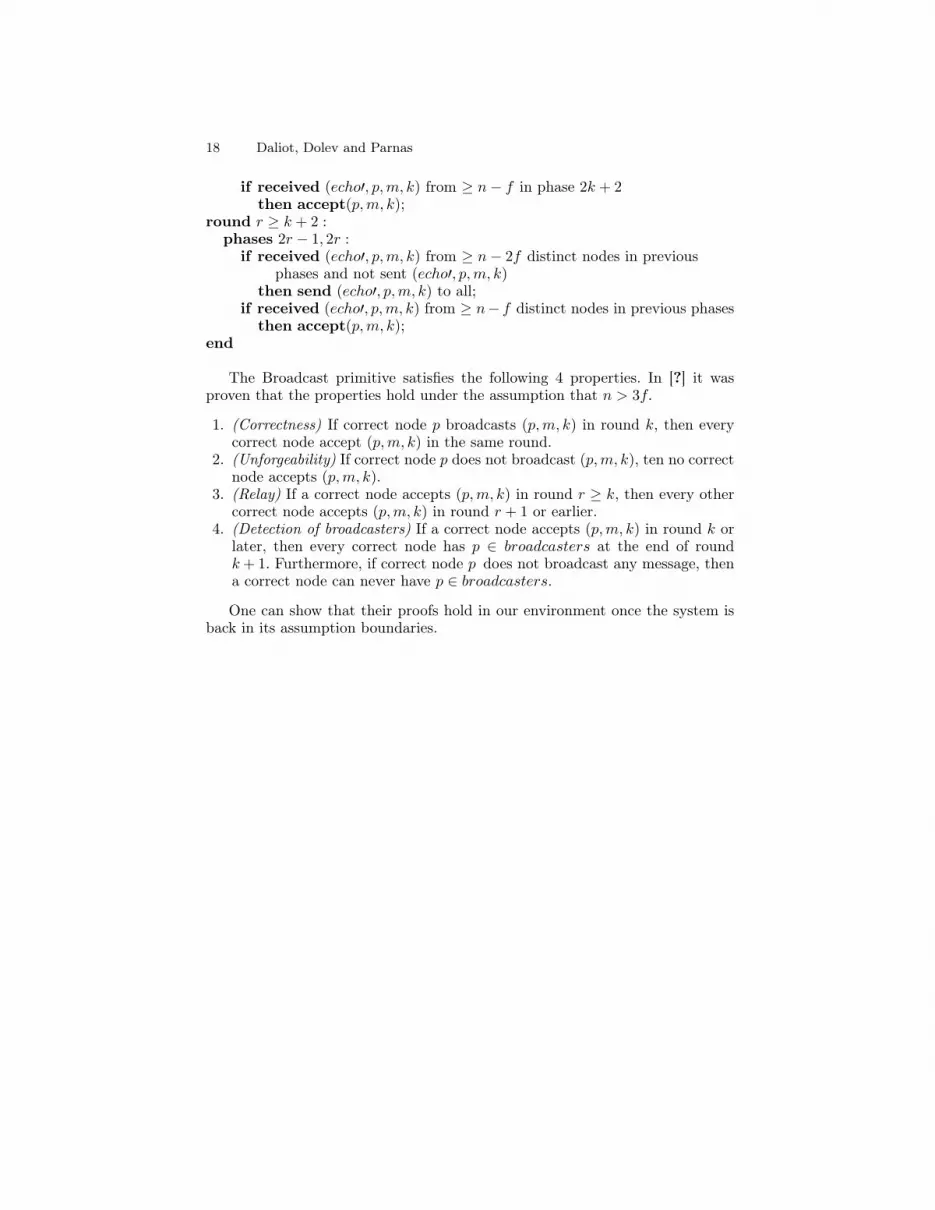
round r ≥ k + 2 :phases 2r − 1, 2r :

if received (echo′, p,m, k) from ≥ n− 2f distinct nodes in previousphases and not sent (echo′, p,m, k)

then send (echo′, p,m, k) to all;if received (echo′, p,m, k) from ≥ n− f distinct nodes in previous phases

then accept(p,m, k);end

The Broadcast primitive satisfies the following 4 properties. In [?] it wasproven that the properties hold under the assumption that n > 3f.

1. (Correctness) If correct node p broadcasts (p,m, k) in round k, then everycorrect node accept (p,m, k) in the same round.

2. (Unforgeability) If correct node p does not broadcast (p,m, k), ten no correctnode accepts (p,m, k).

3. (Relay) If a correct node accepts (p,m, k) in round r ≥ k, then every othercorrect node accepts (p,m, k) in round r + 1 or earlier.

4. (Detection of broadcasters) If a correct node accepts (p,m, k) in round k orlater, then every correct node has p ∈ broadcasters at the end of roundk+ 1. Furthermore, if correct node p does not broadcast any message, thena correct node can never have p ∈ broadcasters.

One can show that their proofs hold in our environment once the system isback in its assumption boundaries.

linear time byzantine self-stabilizing clock synchronization

Documents