Electronic copy available at: http://ssrn.com/abstract=1682896

Is more memory in evolutionary selection

(de)stabilizing?

Cars Hommesa, Tatiana Kiselevaa,

Yuri Kuznetsovb and Miroslav Verbicc

April 21, 2010

a CeNDEF, Department of Economics, University of Amsterdam,

Roetersstraat 11, NL-1018 WB Amsterdam, Netherlands

b Department of Mathematics, Utrecht University,

Budapestlaan 6, NL-3584 CD Utrecht, Netherlands

c Department of Economics, University of Ljubljana

Kardeljeva ploscad 17, SI-1000 Ljubljana, Slovenia

Abstract

We investigate the effects of memory on the stability of evolutionary

selection dynamics based on a multi-nomial logit model in a simple asset

pricing model with heterogeneous beliefs. Whether memory is stabilizing or

destabilizing depends in general on three key factors: (1) whether or not the

weights on past observations are normalized; (2) the ecology or composition

of forecasting rules, in particular the average trend extrapolation factor and

the spread or diversity in biased forecasts, and (3) whether or not costs for

information gathering of economic fundamentals have to be incurred.

JEL classification: C61, D84, E32, G12.

Key Words: fitness measure, asset pricing, bifurcations, evolutionary se-

lection, heterogeneous beliefs, memory strength.

1

Electronic copy available at: http://ssrn.com/abstract=1682896

1 Introduction

Heterogeneous expectations models are becoming increasingly popular in various

fields of economic analysis, such as exchange rate models (De Grauwe et al., 1993;

Da Silva, 2001; De Grauwe and Grimaldi, 2005; 2006), macro-monetary policy

models (Evans and Honkapohja, 2003; Evans and McGough, 2005; Bullard et al.,

2008; Anufriev et al., 2009), overlapping-generations models (Duffy, 1994; Tuinstra,

2003; Tuinstra and Wagener, 2007) and models of socio-economic behaviour (Lux,

1995, Brock and Durlauf, 2001; Alfarano et al., 2005). Yet the application with the

most systematic and perhaps most promising heterogeneous expectations models

seems to be asset price modelling. Contributions of e.g. Brock and Hommes

(1998), Lux and Marchesi (1999), LeBaron (2000), Chiarella and He (2002), Brock

et al. (2005) and Gaunersdorfer et al. (2008) demonstrate how a simple standard

asset pricing model with heterogeneous beliefs is able to lead to complex dynamics

that makes it extremely hard to predict the co-evolution of prices and forecasting

strategies in asset markets. A widely used framework is the adaptive belief systems

(ABS), a financial market application of the evolutionary selection of expectation

rules, introduced by Brock and Hommes (1997). See Hommes (2006) and LeBaron

(2006) for extensive reviews of agent-based models in finance; recent overviews

stressing the empirical and experimental validation of agent-based models are Lux

(2009) and Hommes and Wagener (2009).

An important result in asset pricing models with heterogeneous beliefs is that

non-rational traders, such as technical analysts extrapolating past price trends,

may survive evolutionary competition. These results contradict the hypothesis

that irrational traders will be driven out of the market by rational arbitrageurs,

who trade against them and earn higher profits and accumulate higher wealth

(Friedman, 1953). In most asset pricing models with heterogeneous beliefs, irra-

tional chartists can survive because evolutionary selection is driven by short run

profitability. The role of memory, time horizons or long run profitability in the

2

evolutionary fitness measure underlying strategy selection has hardly been studied

in the literature however.

LeBaron (2001, 2002) are among the few papers that have addressed the role of

investor’s time horizon in learning and strategy selection in an agent-based financial

market. It has been argued that investors’ time horizon is related to whether they

believe that the world is stationary or non-stationary. In a stationary world agents

should use all available information in learning and strategy selection, while if one

views the world as constantly in a state of change, then it will be better to use

a shorter history of past observations. One of LeBaron’s main findings is that

in a world where more agents have a long-memory horizon the volatility of asset

price fluctuations is smaller. Stated differently, long-horizon investors make the

market more stable, while short-horizon investors contribute to excess volatility

and prevent asset prices to converge to the rational, fundamental benchmark.

Another contribution along these lines is Brock and Hommes (1999), who use

a simple, tractable asset pricing model with heterogeneous beliefs to investigate

the effect of memory in the fitness measure for strategy selection. In contrast

to LeBaron (2001, 2002) they find that more memory in strategy selection may

destabilize asset price dynamics1.

Honkapohja and Mitra (2003) provide analytical results for dynamics of adap-

tive learning when the learning rule has finite memory. These authors focus on the

case of learning a stochastic steady state. Although their work is not done in a

heterogeneous agent setting, the results are interesting for our analysis. Their fun-

damental outcome is that the expectational stability principle, which plays a central

role in stability of adaptive learning, as discussed e.g. in Evans and Honkapohja

(2001), retains its importance in the analysis of incomplete learning, though it takes

a new form. Their main result is that expectational stability guarantees stationary

dynamics under learning with finite memory, with unbiased forecasts but higher

price volatility than under complete learning with infinite memory.

1Another related paper is Levy et al. (1994), who simulate an agent-based microscopic stockmarket model with a fixed memory length of 10.

3

Chiarella et al. (2006) study the effect of the time horizon in technical trading

rules upon the stability in a dynamic financial market model with fundamentalists

and chartists. The chartist demand is governed by the difference between the cur-

rent price and a (long-run) moving average. One of their main results is that an

increase of the window length of the moving average rule can destabilize an oth-

erwise stable system, leading to more complicated, even chaotic behaviour. The

analysis of the corresponding stochastic model was able to explain various mar-

ket price phenomena, including temporary bubbles, sudden market crashes, price

resistance and price switching between different levels.

The aim of our paper is to study the role of memory or time horizon in evo-

lutionary strategy selection in a simple, analytically tractable asset pricing model

with heterogeneous beliefs. We shall analyze the effects of additional memory in

the fitness measure on evolutionary adaptive systems and the consequences for

survival of technical trading strategies. By complementing the stability analysis

with local bifurcation theory (see Kuznetsov (2004) for an extensive mathematical

treatment), we will be able to analyze the effects of adding different amounts of

memory to the fitness measure on stability in a standard asset pricing model with

heterogeneous beliefs.

The outline of the paper is as follows. In Chapter 2 an adaptive belief system

is presented in its general form with H different trader types. In Chapter 3 an

ABS with two types and costs for information gathering is examined. In Chapter

4 we investigate the stability of the fundamental steady state in a more generalized

framework without information costs. In Chapter 5 our theoretical findings with

respect to memory are examined numerically in an example with three strategies.

The final section concludes and proofs are collected in an appendix.

4

2 Adaptive Belief Systems

An adaptive belief system is a standard discounted value asset pricing model de-

rived from mean-variance maximization with heterogeneous beliefs about future

asset prices. We shall briefly recall the model as in Brock and Hommes (1998); for

a recent more detailed discussion see e.g. Hommes and Wagener (2009).

2.1 The asset pricing model

Agents can either invest in a risk free asset or in a risky asset. The risk free asset

is in infinite elastic supply and pays a fixed rate of return r; the risky asset is in

fixed supply zs and pays uncertain dividend. Let pt be the price per share of the

risky asset at time t, yt the stochastic dividend process of the risky asset and zt be

the number of shares of risky assets purchased at date t. Then wealth dynamics is

given by

Wt+1 = (1 + r)Wt + (pt+1 + yt+1 − (1 + r)pt) zt. (2.1)

There are H different types of trading strategies. Let Eht and Vht denote forecasts

of trader type h, with h = 1, ..., H, about conditional expectation and conditional

variance, which is based on a publicly available information set of past prices and

past dividends. Demand zh,t of a trader of type h for the risky asset is derived from

myopic mean-variance maximization, i.e.

maxzt

{Eht [Wt+1]−

a

2Vht [Wt+1]

}, (2.2)

where a is the risk aversion parameter. Then the demand zh,t is given by

zh,t =Eh,t[pt+1 + yt+1 − (1 + r)pt]

aVh,t[pt+1 + yt+1 − (1 + r)pt]. (2.3)

5

Let zs denote the supply of outside risky shares per investor, assumed to be con-

stant, and let nh,t denote the fraction of type h at date t. Then equality of the

demand and the supply in the market equilibrium implies

H∑h=1

nhtEh,t[pt+1 + yt+1 − (1 + r)pt]

aVh,t[pt+1 + yt+1 − (1 + r)pt]= zs. (2.4)

We shall assume the conditional variance Vh,t = σ2 to be constant and equal for all

types2, thus the equilibrium pricing equation is given by

(1 + r)pt =H∑

h=1

nh,tEh,t[pt+1 + yt+1]− aσ2zs. (2.5)

As in Brock and Hommes (1998) we focus on the case of zero outside supply,

i.e. zs = 0. It is well known that, if all agents are rational, the asset price is given

by the discounted sum of expected future dividends

p∗t =∞∑

k=1

Et[yt+k]

(1 + r)k. (2.6)

The price p∗t is called the fundamental price. The properties of p∗t depend upon

the stochastic dividend process yt. We focus on the case of IID dividend process yt

with constant mean y, for which the fundamental price is constant and given by

p∗ =∞∑

k=1

y

(1 + r)k=

y

r. (2.7)

It will be convenient to work with the deviation from the fundamental price

xt = pt − p∗. (2.8)

Beliefs of type h satisfy the following assumptions

2Gaunersdorfer (2000) investigates the case with time varying beliefs about variances andshows that the asset price dynamics are quite similar. Chiarella and He (2002, 2003) investigatethe model with heterogeneous risk aversion coefficients.

6

[B1] Vh,t[pt+1 + yt+1 − (1 + r)pt] = σ2,

[B2] Eh,t[yt+1] = Et[yt+1] = y,

[B3] Eh,t[pt+1] = Et[p∗t+1] + fh(xt−1, ..., xt−L) = p∗ + fh(xt−1, ..., xt−L).

Assumption [B1] says that beliefs about conditional variance are equal and constant

for all types. According to assumption [B2] expectations about future dividends

yt+1 are the same and correct for all trader types. According to assumption [B3],

traders of type h believe that in a heterogeneous world the price may deviate from

its fundamental value p∗t by some function fh = fh(xt−1, ..., xt−L) of past deviations.

The function fh represents agent type h’s view of the world.

Brock and Hommes (1998) investigated evolutionary competition between sim-

ple linear forecasting rules with only one lag

fh,t = ghxt−1 + bh, (2.9)

where gh is the trend and bh is the bias of trader type h. If bh = 0 we call an

agent h a pure trend chaser if gh > 0 and a contrarian if gh < 0. In the special

case gh = 0 and bh = 0 trader of type h is a fundamentalist, believing that price

returns to its fundamental value.

An important and convenient consequence of the assumptions [B1]-[B3] is that

the heterogeneous agent market equilibrium (2.5) can be reformulated in devia-

tions from the fundamental price. The fact that the fundamental price satisfies

(1 + r)p∗ = Et[pt+1 + yt+1] yields the equilibrium equation in deviations from the

fundamental value

(1 + r)xt =H∑

h=1

nh,tfh,t. (2.10)

7

2.2 Evolutionary fitness with memory

The evolutionary part of the model describes how beliefs are updated, i.e. how the

fractions nh,t of trader types in the market evolve over time. Fractions are updated

according to an evolutionary fitness measure Uh,t. The fractions of agents choosing

strategy h are given by the multi-nomial logit probabilities

nh,t =exp(βUh,t−1)∑H

h=1 exp(βUh,t−1). (2.11)

The intensity of choice parameter β ≥ 0 measures how sensitive the traders are to

selecting the optimal prediction strategy. The extreme case β = 0 corresponds to

the case where agents do not switch and all fractions are fixed and equal 1/H. The

other extreme case β = ∞ corresponds to the case where all traders immediately

switch to the optimal strategy. An increase in the intensity of choice β represents

an increase in the degree of rationality with respect to evolutionary selection of

trading strategies. One of the main results of Brock and Hommes (1998) is that a

rational route to randomness occurs, that is, as the intensity of choice increases the

fundamental steady state becomes unstable and a bifurcation route to complicated,

chaotic asset price fluctuations arises. The key question to be addressed in this

paper is whether more memory is stabilizing or destabilizing. In particular, we are

interested in the question how memory in the fitness measure affects the primary

bifurcation towards instability and how it affects the rational route to randomness.

A natural candidate for evolutionary fitness is a weighted average of current

realized profits πht and last period fitness Uh,t−1

Uh,t = γπh,t + wUh,t−1

= γ

[(pt + yt −Rpt−1)

Eh,t−1[pt + yt −Rpt−1]

aσ2− Ch

]+ wUh,t−1, (2.12)

where R = 1 + r, Ch ≥ 0 is an average per period cost of obtaining forecasting

strategy h, and w ∈ [0, 1) is a memory parameter measuring how quickly past

8

realized fitness is discounted for strategy selection. The parameter γ in (2.12) has

been introduced to distinguish between two important cases in the literature. Brock

and Hommes (1998) proposed the case γ = 1, implying that the weights given to

past profits decline exponentially, more precisely realized profit k−periods ago gets

weight wk; Brock and Hommes (1998) however, as well as almost all subsequent

literature, focus the analysis on the case without memory, i.e., w = 0, with fitness

equal to current realized profit3. An advantage of the case γ = 1 is that w = 1

corresponds to the benchmark where fitness equals the accumulated excess profit

of the risky asset over the risk free asset4. A disadvantage however is that for γ = 1

the weights are not normalized, but rather sum up to 1/(1− w). The second case

studied in the literature assumes γ = 1 − w, corresponding to the case where the

weights are normalized and add up to 1. Note that for w = 1/T and γ = 1− 1/T ,

this case reduces to a T−period average with fixed T (see e.g. LeBaron (2001) and

Diks and van der Weide (2005)). We will refer to the case γ = 1 as cumulative

weights and to the case γ = 1− w as normalized weights5.

Notice that the two different cases lead to the same distribution of the relative

weights over past profits, given by (1, w, w2, w3, · · · ). Stated differently, the relative

contribution of past profits to overall fitness is the same for both weighting schemes.

For both weighting schemes, an increase of w thus means an increase of memory

in the sense that more weight is given to more distant observations. However, an

increase of w has another, second effect which is different for the two weighting

schemes. As stated above, for γ = 1 all weights add up to 1/(1 − w), while for

γ = 1− w the weights are normalized to 1. This implies a scaling effect for γ = 1,

with the sum of the weights, 1/(1 − w), blowing up to infinity as w approaches

3It is interesting to note that Anufriev and Hommes (2009) fit an evolutionary selection modelto data from laboratory experiments and use a memory parameter w = 0.7.

4There is a large related literature on wealth-driven selection models with heterogeneous in-vestors, with fractions of each type determined by relative wealth. See e.g. Anufriev (2008) andAnufriev and Bottazzi (2006) for some recent contributions and Chiarella et al. (2009) and Hensand Schenk-Hoppe (2009) for extensive up to date reviews.

5This terminology is similar to that used in the experience-weighted attraction (EWA) learningin games literature (e.g. Camerer and Ho (1999) and Camerer (2003)), where a parameter movesfrom 0 to 1 between the extremes of cumulative and average reinforcement.

9

1. In particular, for γ = 1 the fitness at steady state is multiplied by a factor

1/(1−w). Hence, for the stability of a steady state, this scaling effect for γ = 1 is

equivalent to an increase of the intensity of choice β by a factor 1/(1−w). Because

an increase of the intensity of choice may be destabilizing (Brock and Hommes,

1997, 1998) the scaling effect for γ = 1 may be a destabilizing force as w increases,

not present in the case of normalized weights. Another, related way of looking at

this is to consider the direct effect of current realized profits on fitness. In the case

of normalized weights, γ = 1 − w, the direct effect of current realized profits πht

(getting weight 1−w) on fitness vanishes, i.e. tends to 0, as w tends to 1. On the

other hand, in the case of cumulative weights, γ = 1, the direct effect of current

realized profits πht (always getting weight 1) on fitness stays the same, and thus

remains non-negligible, independent of w. As we will see, these differences will lead

to different stability results for evolutionary selection6.

Fitness (2.12) can be rewritten in deviations from the fundamental as

Uh,t = γ

[(xt −Rxt−1 + δt)

(ghxt−2 + bh −Rxt−1

aσ2

)− Ch

]+ wUh,t−1, (2.13)

with δt = p∗t + yt − Et−1[p∗t + yt] a martingale difference sequence, representing

intrinsic uncertainty about economic fundamentals. The Adaptive Belief System

(ABS) with linear forecasting rules, in deviations from the fundamental, is given

6The difference between cumulative weights versus normalized weights as expressed throughthe weighting coefficients γ = 1 versus γ = 1−w is related to the more general issue of cumulativeversus normalized fitness measure Uh,t; see the final Section for more discussion.

10

by

(1 + r)xt =H∑

h=1

nh,t (gixt−1 + bi) + εt, (2.14)

nh,t =exp(βUh,t−1)

H∑h=1

exp(βUh,t−1)

, (2.15)

Uh,t = γ

[(xt −Rxt−1 + δt)

(ghxt−2 + bh −Rxt−1

aσ2

)− Ch

]+ wUh,t−1,

(2.16)

where an additional noise term εt, e.g. representing a small fraction of noise traders,

has been added to the pricing equation and will be used in some stochastic simula-

tions below. A special case, the deterministic skeleton, arises when all noise terms

are set to zero. In order to understand the properties of the general stochastic

model it is important to understand the properties of the deterministic skeleton.

3 Two types of agents and information costs

Consider an Adaptive Belief System (ABS) with two types of traders and the

following forecasting rules

f1,t = g1xt−1, 0 ≤ g1 < 1,

f2,t = g2xt−1, 1 < g2.(3.1)

Type 1 believes in mean reversion, that the price will converge to its fundamental

value. In the special case g1 = 0, type 1 becomes a pure fundamentalists, as in

Brock and Hommes (1998). In contrast, type 2 believes that price deviations from

the fundamental are persistent and will increase7. The dynamics in deviations from

7Boswijk et al. (2007) estimated this ABS with two types of investors using yearly S&P 500data and found coefficients of g1 ≈ 0.8 and g2 ≈ 1.15, thus suggesting behavioral heterogeneity.

11

the fundamental is described by the following system

Rxt = n1,tg1xt−1 + n2,tg2xt−1, (3.2)

nh,t =exp (βUh,t−1)∑2

h=1 exp (βUh,t−1), (3.3)

Uh,t−1 = γ

[(xt−1 −Rxt−2)

(ghxt−3 −Rxt−2

d

)− Ch

]+ wUh,t−2, (3.4)

where C2 = 0, but C1 = C > 0 is the information gathering costs for fundamen-

talists that agents of type 1 must pay per period. These costs reflect the effort

investors incur to collect information about economic fundamentals.

We can rewrite the system above as a five-dimensional map

xt−1

xt−2

xt−3

U1,t−2

U2,t−2

7→

1R(n1,tg1 + n2,tg2)xt−1

xt−1

xt−2

γπ1,t−1 + wU1,t−2

γπ2,t−1 + wU2,t−2

. (3.5)

The following theorem describes the results concerning existence and stability of

the steady states (see Appendix A for the proof).

Theorem 3.1. (Existence and stability of the steady states) Let us denote

the fundamental steady state as xf = 0, and non-fundamental steady states as

x+ = x∗ > 0 and x− = −x∗ < 0, where

x∗ =

√√√√C − 1−wγβ

log(R−g1

g2−R)

(R− 1)g2−g1

aσ2

, C > 0. (3.6)

Let

β∗ =1− w

Cγlog

R− g1

g2 −R. (3.7)

Then three cases are possible:

12

(i) 1 < g2 < R: the fundamental steady state xf is the unique steady state and

it is globally stable;

(ii) R ≤ g2 < 2R− g1, the system displays a pitchfork bifurcation at β = β∗ such

that

– for 0 < β < β∗ xf is unique and stable;

– for β > β∗ there are three steady states: xf , x+ and x−; the fundamental

steady state xf is unstable;

(iii) g2 ≥ 2R − g1: there are always three steady states: xf , x+ and x−; the

fundamental steady state xf is unstable.

When the trend chasers extrapolate only weakly, i.e. 1 < g2 < R, the funda-

mental steady state xf = 0 is globally stable. If C = 0 then the two types of agents

are equally represented in the market, i.e. n1 = n2 = 1/2 for any value of β, because

the difference in fitnesses U2 − U1 = 0 at x = 0. If agents on average extrapolate

very strongly, i.e. (g1 + g2)/2 > R, the fundamental steady state is unstable and

there are always two additional non-fundamental steady states x = x+ > 0 and

x = x− < 0, even when there are no information costs. The case with strongly

extrapolating trend chasers, i.e. R < g2 < 2R− g1, is the most interesting. If there

are no information costs, C = 0, the fundamental steady state is stable for all

values of β and agents are equally distributed over the two types due to equality of

profits. But when C > 0 the fundamental steady state is stable only if the agents

are not too sensitive to switch the prediction strategy, i.e. for β < β∗. As the

intensity of choice increases (β > β∗) most of the agents switch to use the cheap

prediction rule, because if the price is in a small neighborhood of its fundamental

value then due to information costs the first type of agents have lower profits and

for large β a majority of agents switches to the trend extrapolating strategy.

It can be seen immediately from expressions (3.6) and (3.7) how memory affects

the primary bifurcation of the system. In the case with normalized weights (γ = 1−

13

w) memory does not affect the stability. However, in the case of cumulative weights

(γ = 1) and positive information gathering costs for fundamentalists, memory does

affect the stability and in fact it destabilizes the system, i.e. with more memory

the primary bifurcation occurs earlier. This is due to a scaling effect when the

parameter w increases, leading to a larger effective intensity of choice and thus to

an earlier bifurcation of the fundamental steady state.

Simulation 2 type example

As a typical example consider an ABS with the following two prediction rules

f1,t = 0.5xt−1, (3.8)

f2,t = 1.2xt−1. (3.9)

Traders of the first type believe that the next period deviation of the price from

the fundamental will be two times less than in the current period, whereas traders

of the second type predict an increase in deviation of the price from fundamental.

It follows from Theorem 3.1 that the fundamental steady state xf = 0 is unique

and stable for β ∈ (0, β∗), with β∗(w) = 1.79(1 − w)/γ. When the parameter β

passes the critical value β∗, the fundamental steady state looses stability due to a

pitchfork bifurcation and two new stable equilibria of the price dynamics appear.

Next consider the two different cases: cumulative versus normalized weights.

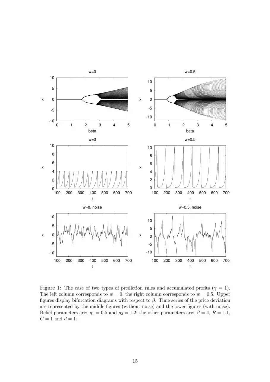
Cumulative weights (γ = 1). In the case with accumulated profits, i.e. when

γ = 1, the pitchfork bifurcation curve is given by β∗(w) = 1.79(1−w), which is de-

clining with respect to the memory parameter. It means that memory destabilizes

the price dynamics: the larger w the earlier the primary bifurcation occurs.

Fig. 1 illustrates the dynamics without memory (w = 0, left panel) and with

memory (w = 0.5, right panel). In both cases a rational route to randomness, that

is, a bifurcation route to complicated dynamics as the intensity of choice increases,

14

-10

-5

0

5

10

0 1 2 3 4 5

x

beta

w=0

-10

-5

0

5

10

0 1 2 3 4 5

x

beta

w=0.5

0

2

4

6

8

10

100 200 300 400 500 600 700

x

t

w=0

0

2

4

6

8

10

100 200 300 400 500 600 700

x

t

w=0.5

-10

-5

0

5

10

100 200 300 400 500 600 700

x

t

w=0, noise

-10

-5

0

5

10

100 200 300 400 500 600 700

x

t

w=0.5, noise

Figure 1: The case of two types of prediction rules and accumulated profits (γ = 1).The left column corresponds to w = 0, the right column corresponds to w = 0.5. Upperfigures display bifurcation diagrams with respect to β. Time series of the price deviationare represented by the middle figures (without noise) and the lower figures (with noise).Belief parameters are: g1 = 0.5 and g2 = 1.2; the other parameters are: β = 4, R = 1.1,C = 1 and d = 1.

15

-10

-5

0

5

10

0 1 2 3 4 5

x

beta

w=0

-10

-5

0

5

10

0 1 2 3 4 5

x

beta

w=0.5

0

2

4

6

8

10

100 200 300 400 500 600 700

x

t

w=0

0

2

4

6

8

10

100 200 300 400 500 600 700

x

t

w=0.5

-10

-5

0

5

10

100 200 300 400 500 600 700

x

t

w=0, noise

-10

-5

0

5

10

100 200 300 400 500 600 700

x

t

w=0.5, noise

Figure 2: The normalized fitness measure case (γ = 1 − w): time series of the pricedeviation from its fundamental value for different levels of the memory. Belief parametersare: g1 = 0.5 and g2 = 1.2; the other parameters are: β = 4, R = 1.1, C = 1 and d = 1.

16

occurs. Notice that, with memory in the fitness measure, the temporary bubbles

and crashes in the price series occur less frequently, but when they occur they last

longer with much larger deviations from the fundamental benchmark.

Normalized weights (γ = 1−w). In the case with normalized weights, i.e. when

γ = 1−w, the pitchfork bifurcation curve is given by β∗(w) = 1.79. Hence, memory

does not affect the stability of the fundamental steady state. Fig. 2 illustrates

the dynamics without memory (w = 0, left panel) and with memory (w = 0.8,

right panel). Although less pronounced, memory has a similar effect on price

fluctuations: with memory in the fitness measure, the temporary bubbles and

crashes in the price series occur less frequently, but once started bubbles last longer

with larger swings away from the fundamental benchmark.

The bottom panels of Figures 1 and 2 contain time series simulations in the

presence of noise, represented by a small fraction of noise traders. While in the

deterministic simulations the chaotic bubbles and crashes are still somewhat pre-

dictable, in the presence of noise they become very irregular and highly unpre-

dictable.

4 Stability in the model with H types

Brock and Hommes (1998) stressed the importance of simple forecasting rules,

because it is unlikely that enough traders will coordinate on a complicated rule

for it to have an impact in real markets. The learning to forecast laboratory

experiments of Hommes et al. (2005) show that simple, linear forecasting rules

with only a few lags describe individual forecasting behavior surprisingly well. In

this section, we investigate the role of memory in an ABS with an arbitrary number

H of linear forecasting rules with one lag, i.e.

fi,t = gixt−1 + bi, gi, bi ∈ R, i = 1, . . . , H, (4.1)

17

and without information gathering costs, i.e. Ci = 0 for all i=1,. . . ,H. The co-

evolution prices and beliefs is described by the following difference equation

Rxt =H∑

h=1

nh,t (ghxt−1 + bh) , (4.2)

nh,t =exp (βUh,t−1)∑H

h=1 exp (βUh,t−1), (4.3)

Uh,t−1 = γ

[(xt−1 −Rxt−2)

(ghxt−3 + bh −Rxt−2

d

)]+ wUh,t−2

= γπh,t + wUh,t−2. (4.4)

with d = aσ2. Equation (4.2) can be rewritten as a (H+3)-dimensional map

xt−1

xt−2

xt−3

U1,t−2

· · ·

UH,t−2

7→

1R

∑Hh=1 nh,t(ghxt−1 + bh)

xt−1

xt−2

γπ1,t−1 + wU1,t−2

· · ·

γπH,t−1 + wUH,t−2

. (4.5)

The following theorem describes the results concerning existence and stability

of the fundamental steady state (see Appendix B for the proof).

Theorem 4.1. (Existence and stability of the fundamental steady state)

Assume that

1. The average bias equals zero, i.e.,∑H

i=1 bi = 0;

2. There is at least one non-zero bias, i.e. V = 1H

∑Hi=1 b2

i > 0;

3. The mean trend is not too strong, i.e. |g| = | 1H

∑Hi=1 gi| < R.

Then the fundamental price xf = 0 is a steady state of (4.5). The fundamental

18

steady state is stable for 0 ≤ β < βNS, where

βNS =aσ2

V γ(1− g

Rw) > 0. (4.6)

At the value β = βNS the steady state loses stability due to a Neimark-Sacker

bifurcation. For β > βNS the fundamental steady state is unstable8.

The assumptions that the average bias is zero seems reasonable, as there is no

a priori reason why the average bias would be negative or positive9. The other two

assumptions, that there is at least one non-zero bias and that the average trend over

all rules is not too strong, also seem plausible. The theorem says that, under these

assumptions, the dynamic behavior of the price of the risky asset is independent

of the number of agent’s strategies, but rather depends on the mean value g of

the trend extrapolating coefficients gh and the diversity or spread V of the biases

bh. The larger the absolute average trend |g|, the lower βNS and the earlier the

primary bifurcation occurs; if the trend chasers on average extrapolate more heavily

away from the fundamentals, the system destabilizes faster. Similarly, the greater

the variance V in biases, the lower βNS and the bifurcation again occurs earlier; if

there is more variability among biased traders, the price dynamics becomes unstable

earlier. Note that for the special case g = 0 and γ = 1, memory does not affect

the stability of the fundamental steady state, since βNS = aσ2/V (cf. Brock and

Hommes, 1998).

Role of the parameter γ. In the case γ = 1, i.e. in the case of cumulative

weights, the Neimark-Sacker bifurcation curve (4.6) becomes a straight line

βNS =aσ2

V

(1− g

Rw

), (4.7)

8Note that in the special case V = 0 all biases equal zero, and if |g| < R the fundamentalsteady state is stable for all values of β and w.

9If the average bias is non-zero and close to 0, the fundamental price is not a steady state butthe system has a steady state close to the fundamental. In that case, a stability analysis becomesmuch more cumbersome however.

19

as illustrated in Figure 3 (left panel). The slope of the line depends on the sign of

the average trend extrapolation g. If agents on average extrapolate positively, then

the line is decreasing and the bifurcation w.r.t. β comes earlier with more memory.

The intuition is that positive trend extrapolation reinforces market movements

away from the fundamentals and the system destabilizes faster. On the other

hand, if agents on average are contrarians extrapolating negatively, then (4.7) is an

increasing line and the bifurcation w.r.t. β comes later with more memory. Here

the intuition is that contrarian behavior counter-balances market movements away

from the fundamentals and the system destabilizes slower.

0 0.2 0.4 0.6 0.8 1w0

20

40

60

���1

0 0.2 0.4 0.6 0.8 1w0

100

200

300

400

���1�w

Figure 3: Neimark-Sacker bifurcation curves βNS in (4.6) for different values of theparameters γ and g: dotted lines correspond to the case g > 0, while solid lines correspondto the case g < 0. For the case with γ = 1 (left panel) the bifurcation curves are straightlines, whereas for γ = 1 − w (right panel) they are hyperbolas. In the case γ = 1 (leftpanel) and g > 0 memory has a destabilizing effect on the dynamics, i.e. the bifurcationw.r.t. β comes earlier. In contrast, in the case γ = 1 − w (right panel) more memoryalways has a stabilizing effect.

In the case with normalized weights, γ = 1−w, the Neimark-Sacker bifurcation

curve (4.6) becomes a “hyperbola” for both positive and negative values of g (see

Figure 3, right panel):

βNS =aσ2

V (1− w)(1− g

Rw). (4.8)

In the case of normalized weights, memory is always stabilizing (independent of

the average extrapolation factor g). Notice that the Neimark-Sacker bifurcations

values (4.7) and (4.8) only differ by a factor (1 − w) in the denominator of (4.8)

20

representing the scaling effect when weights are not normalized. Comparing the

left and right panels of Figure 3, this scaling effect dominates when average trend

extrapolation g > 0 and destabilizes the system when the memory parameter w

increases in the case of cumulative weights (i.e. γ = 1).

5 Numerical simulation of a 3-type example

In this section we discuss a simple, but typical ABS with three types of traders

in order to illustrate the differences in impact of the memory strength on the

stability of the fundamental price in the two cases of cumulative weights (γ = 1)

and normalized weights (γ = 1− w).

Consider the ABS with the following three types of prediction rules

f1,t = 0, (5.1)

f2,t = 1.2xt−1 − 0.2, (5.2)

f3,t = 0.9xt−1 + 0.2. (5.3)

The second and the third types are symmetrically opposite biased positive trend

extrapolators, the first type are fundamentalists. The remaining parameters are

fixed at: R = 1.1, aσ2 = 1. Since g = 0.7 < R, V = 0.08/3 6= 0 and biases sum up

to zero, according to Theorem 4.1, the fundamental steady state looses stability in

a Neimark-Sacker bifurcation at β = βNS,

βNS =37.5− 23.9w

γ. (5.4)

The case γ = 1. In the case with cumulative weights, i.e. when γ = 1, the

Neimark-Sacker bifurcation curve is a declining straight line:

βNS = 37.5− 23.9w. (5.5)

21

0 0.2 0.4 0.6 0.8 1w0

20

40

�

stable

unstable

Figure 4: Neimark-Sacker bifurcation curve (left panel) and bifurcation diagram withrespect to the memory parameter w (right panel) for the model with three types ofagents and fitness given by accumulated profits, i.e. γ = 1. Belief parameters are:g1 = 0, b1 = 0; g2 = 1.1, b2 = −0.2; and g3 = 0.9, b3 = 0.2; other parameters are:R = 1.1, aσ2 = 1 and β = 25 (for the right panel). The Neimark-Sacker bifurcation curvedivides the (w, β)−plane into two regions; for the parameter values in the upper regionthe fundamental steady state is unstable, while for the parameter values in the lowerregion it is stable.

As can be seen from Figure 4, in this case memory destabilizes the price dynamics;

with higher memory strength the bifurcation occurs earlier, i.e. for smaller values

of β. Since both non-fundamentalist agents extrapolate positively, and thus the

average trend extrapolation is also positive, in accordance with our findings from

Section 4, the extrapolation of trend reinforces markets movements away from the

fundamentals and the bifurcation line is thus decreasing. In addition, it can be ob-

served in the bifurcation diagram of Figure 4 (right panel) how, for a fixed β-value,

the fundamental steady state becomes unstable and complicated, chaotic price

movements arise as the memory parameter w increases. Figure 4 (right panel) also

illustrates that the amplitude of price fluctuation increases as memory increases,

in accordance with our earlier finding that bubbles last longer with more memory.

The case γ = 1− w. In the case with normalized weights, i.e. when γ = 1− w,

the Neimark-Sacker bifurcation curve (5.4) becomes a “hyperbola”:

βNS =37.5− 23.9w

1− w. (5.6)

22

0 0.2 0.4 0.6 0.8 1w0

100

200

�

stable

unstable

Figure 5: Neimark-Sacker bifurcation curve (left) and bifurcation diagram with respectto the memory (right) for the model with three types of agents’ strategies and normalizedfitness measure, i.e. γ = 1−w. Belief parameters are: g1 = 0, b1 = 0; g2 = 1.1, b2 = −0.2;and g3 = 0.9, b3 = 0.2; other parameters are: R = 1.1, d = 1 and β = 70 (for the rightfigure). The Neimark-Sacker bifurcation curve divides the (w, β)−plane into two regions;for the parameter values in the upper region the fundamental steady state is unstable,while for the parameter values in the lower region it is stable.

As can be seen from Figure 5 (left panel), more memory now stabilizes the

price dynamics; an increase in the memory strength makes the bifurcation occur

later, i.e. for larger values of β. Even when the traders are on average positive

trend extrapolators (with some bias), if the weight on cumulative past fitness (the

memory strength w) is high enough compared to the weight on current realized

profits (γ = 1 − w), the dynamics is stable. Indeed the bifurcation diagram in

Figure 5 (right panel) shows that, for a given β, the dynamics stabilizes from

chaotic movements (interspersed with stable cycles) for low values of the memory

parameter w to a stable fundamental steady state when memory w is sufficiently

large.

6 Conclusion

We investigated how memory affects the stability of evolutionary selection dynamics

in a simple, analytically tractable asset pricing model with heterogeneous beliefs.

By complementing the stability analysis with local bifurcation theory, we were

able to analyze the effects of adding different amounts of memory to the fitness

23

measure on the stability of the fundamental steady state. Whether memory is

stabilizing or destabilizing depends on three key factors: (1) whether we have a

fitness measure with cumulative weights or normalized weights; (2) the ecology (i.e.

the composition of the set) of forecasting rules, in particular the average strength

of trend extrapolation and the spread in biased forecasts, and (3) whether or not

costs for information gathering of economic fundamentals have to be incurred.

When there are costs for gathering fundamental information, more memory in

the fitness measure does not stabilize the dynamics. In the case with normalized

weights, due to the information gathering costs, memory has no effect on stability;

in the case of cumulative weights, when there are information gathering costs for

fundamentalists, more memory is destabilizing due to a scaling effect leading to a

larger effective intensity of choice.

We have also studied the model with an arbitrary number of linear forecasting

rules with one lag and no costs for information gathering. The stability depends

critically on the ecology of forecasting rules. In particular, the system may be-

come unstable more easily when the average trend parameter and or the variability

of biased forecasts become larger. How memory affects the stability of the fun-

damental steady state depends again on whether we have cumulative weights or

normalized weights. In the case of normalized weights, more memory is always

stabilizing: with more memory the first bifurcation towards instability comes later.

In the case of cumulative weights the effect of memory on the stability depends on

the direction of average trend extrapolation. If agents on average are contrarians,

extrapolating negatively, more memory stabilizes the system; if on the other hand

agents on average extrapolate positively, memory destabilizes the system. This is

due to a dominating scaling effect on the fitness at steady state, when weights are

cumulative, which destabilizes the system if average trend extrapolation is positive.

Our analysis yields a precise mathematical classification of the stability of evo-

lutionary selection for cumulative versus normalized weights in the fitness measure

within in a very simple modeling framework. Which of these two fitness measures

24

is more relevant in reality is an empirical and behavioral question. Is individual

choice, for example individual portfolio selection in financial markets, driven by

cumulative fitness (e.g. accumulated wealth) or by normalized fitness (e.g. average

realized returns)? In particular, how much weight do individuals put on the most

recently observed fitness? Our theoretical results show that the more weight they

put on the most recent observation, the more easily the system may destabilize.

Future research with laboratory experiments with human subjects may shed light

on which behavioral assumptions fit individual decision making in strategy selec-

tion more closely and, in particular, how much weight individuals put on most

recent observations.

The difference between cumulative versus normalized weights, as expressed

through the weighting coefficients γ = 1 versus γ = 1 − w, is related to the more

general issue of whether one should use a cumulative or normalized fitness measure

in strategy switching models. An advantage of normalization is that one can com-

pare the magnitude of the intensity of choice parameter across different normalized

fitness measures and market settings. The intensity of choice parameter is notori-

ously hard to estimate and only few significant results have been obtained. Boswijk

et al. (2007) estimate the intensity of choice in an asset pricing model with het-

erogeneous beliefs using yearly S&P500 data, while Goldbaum and Mizrach (2008)

estimate the intensity of choice in mutual fund allocation decisions. Our results

stress the importance of normalization of the fitness measure in empirical appli-

cations. But in general it is not clear, how exactly a fitness measure should be

normalized, especially when the fitness (such as realized profits) may attain (ar-

bitrarily large) positive as well as negative values. The normalization itself may

affect e.g. the primary bifurcation towards instability. Laboratory experiments on

individual selection among different strategies with a normalized fitness measure

may give useful estimates of the intensity of choice of individual strategy selection

across different market settings.

25

A Proof of Theorem 3.1

The steady states of the map (3.5) satisfy the following equation

Rx = x

(g1

1 + exp(β∆)+

g2

1 + exp(−β∆)

)(A.1)

where ∆ =γ

1− w

[(1−R)

(g2 − g1

d

)x2 + C

].

It is easy to see that the fundamental steady state xf = 0 always exists. The

other (non-fundamental) steady state is a solution of the equation

exp

[β

γ

1− w

((1−R)

g2 − g1

dx2 + C

)]=

R− g1

g2 −R. (A.2)

Note that if (R − g1)/(g2 − R) ≤ 0 there are no solutions for this equation. If we

take into account that g1 < 1 then we can conclude that for 1 < g2 < R the map

(3.2)-(3.4) is contracting and has a unique globally stable steady state xf = 0.

Assume now that g2 > R, then we can obtain non-fundamental steady states

from the equation

x2 =C − 1−w

βγln R−g1

g2−R

(R− 1)g2−g1

d

, (A.3)

which has solutions x = ±x∗, when its right hand side is positive. It is satisfied for

β > β∗ in (3.7) if R ≤ g2 < 2R − g1, and for any positive β if g2 ≥ 2R − g1. This

proves the statements about existence of equilibria in (i), (ii) and (iii).

In order to explore the stability of the fundamental steady state we need to

26

compute eigenvalues of the Jacobian matrix

J(xf ) =

g1+g2 exp( Cβγ1−w

)

(1+exp( Cβγ1−w

))R0 0 0 0

1 0 0 0 0

0 1 0 0 0

0 0 0 w 0

0 0 0 0 w

. (A.4)

The characteristic equation is given by

(w − λ)2λ2

(g1 exp

(−Cγβ

1− w

)+ g2 −Rλ

(1 + exp

(−Cγβ

1− w

)))(A.5)

and thus

λ1,2 = 0, λ3,4 = w, λ5 =

g1 exp

(−Cγβ

1− w

)+ g2

R

(1 + exp

(−Cγβ

1− w

)) > 0. (A.6)

Note that all eigenvalues are real and non-negative, so the only bifurcation that

may occur is a pitchfork bifurcation, which happens if

λ5 = 1 ⇔ β = β∗. (A.7)

This means that if g2 ∈ [R, 2R − g1) for β ∈ (0, β∗) there exists a unique stable

fundamental steady state, and at the critical parameter value β = β∗ two non-

fundamental steady states occur due to a pitchfork bifurcation.

B Proof of Theorem 4.1

Note that at the fundamental steady state all fitnesses are equal to zero, i.e. U∗h = 0

for h = 1, .., H, which implies that all fraction are equal, n∗h = 1/H. Therefore the

27

steady state price satisfies the following equation

Rx∗ =1

H

H∑h=1

(ghx∗ + bh) (B.1)

and thus

x∗ (R− g) =1

H

H∑h=1

bh. (B.2)

It is clear that the fundamental steady state exists if and only if∑H

h=1 bh = 0.

The Jacobian of (4.5) computed at the fundamental steady state is given by

dg+V γβd

−V γβd

0 J1,1 · · · J1,H

1 0 0 0 · · · 0

0 1 0 0 · · · 0

b1γd

− b1Rγd

0 w 0 · · · 0

b2γd

− b2Rγd

0 0 w 0 · · · 0

.... . .

bHγd

− bHRγd

0 0 · · · 0 w

where d = aσ2 and

J1,s = −bswβ

HR, s = 1, . . . , H.

The characteristic equation for the fundamental steady state is given by

λ2(w − λ)H−1[dwg + RβV γ + (−d(g + Rw)− βV γ)λ + dRλ2

]︸ ︷︷ ︸p(λ)

= 0. (B.3)

The characteristic equation (B.3) has H+3 roots, where H+1 of them are inside

the unit circle; λ3 = λ4 = 0 and λ5 = . . . = λH+3 = w < 1, while the other two are

roots of the polynomial p(λ) and thus they determine stability of the steady state.

If p(λ) has at least one root outside of the unit circle, the steady state is unstable.

We denote roots of p(λ) as λ1 and λ2.

28

Let us now explore three cases when one or two roots of p(λ) are crossing a unit

circle:

1. λ1 = 1, pitchfork bifurcation,

p(1) = 9d(R− g)(1− w) + 9V (R− 1)γβ.

If V = 0 then p(1) > 0 for w ∈ [0, 1) and |g| < R. If V > 0 then

p(1) = 0 ⇔ β =d(1− w)(g −R)

V (R− 1)γ< 0 for g < R, (B.4)

which means that this type of bifurcation cannot occur in the system.

2. λ1 = −1, period doubling bifurcation,

p(−1) = 9d(R + g)(1 + w) + 9V (R + 1)γβ.

If V = 0 then p(−1) > 0 for w ∈ [0, 1) and |g| < R. If V > 0 then

p(−1) = 0 ⇔ β = βPD = − 4(g + R)(1 + w)

V (1 + R)(1− w)< 0,

which means that this type of bifurcation can not occur in the system either.

3. λ1,2 = µ1 ± µ2i, where µ2 > 0 and µ21 + µ2

2 = 1, Neimark-Sacker bifurcation.

Using Vieta’s Formula we get

µ21 + µ2

2 = λ1λ2 =dgw + RV βγ

dR= 1. (B.5)

If V = 0, the equation (B.5) does not have solutions for w ∈ [0, 1) and

|g| < R. Therefore all eigenvalues corresponding to the fundamental steady

state are inside the unit circle and thus the steady state is stable for w ∈ [0, 1)

and β ≥ 0.

29

If V > 0, we obtain from (B.5) the equation of the Neimark-Sacker bifurcation

curve

βNS =d

V γ(1− g

Rw). (B.6)

We have to make sure that µ2 6= 0 or equally µ22 > 0. Since µ2

1 + µ22 = 1 the

latter inequality holds if µ21 < 1. Using again the Vieta’s Formula we have

µ1 =λ1 + λ2

2=

d(g + Rw) + βV γ

2dR> 0.

To make sure that µ21 < 1 we need to check the inequality

d(g + Rw) + V βγ

2dR< 1.

Together with (B.6) it implies

w(R2 − g) < R(2R− 1− g), (B.7)

which is satisfied for |g| < R and any value of w ∈ [0, 1).

Our analysis shows that the Neimark-Sacker bifurcation is the only bifurcation that

occurs in the system. It happens for β = βNS as in (B.6) and leads to a loss of

stability of the fundamental steady state.

30

References

[1] Anufriev, M. (2008), Wealth driven competition in a speculative financial mar-

ket: examples with maximizing agents, Quantitative Finance 8, 363380.

[2] Anufriev, M. and Bottazzi (2006), Equilibria, stability and asymptotic domi-

nace in a speculative market with heterogeneous agents, Journal of Economic

Dynamics and Control 30, 1787-1835.

[3] Anufriev, M. and Hommes, C.H. (2009), Evolution of market heuristics,

Knowledge Engineering Review, forthcoming.

[4] Alfarano, S., Lux, T. and Wagner, F., (2005) Estimation of Agent-Based Mod-

els: The Case of an Asymmetric Herding Model. Computational Economics,

26 (1): 19-49.

[5] Anufriev, M., Assenza, T. Hommes, C. and Massaro, D. (2009), Interest Rate

Rules and Macroeconomic Stability under Heterogeneous Expectations, CeN-

DEF working paper, University of Amsterdam, February 2009.

[6] Brock, W. A. and Durlauf, S. N., (2001) Discrete Choice with Social Interac-

tions. Review of Economic Studies, 68 (2): 235-260.

[7] Boswijk, H.P., Hommes, C.H. and Manzan, S. (2007), Behavioral heterogene-

ity in stock prices, Journal of Economic Dynamics and Control 31, 1938-1970.

[8] Brock, W. A. and Hommes, C. H., (1997) A Rational Route to Randomness.

Econometrica, 65 (5): 1059-1095.

[9] Brock, W. A. and Hommes, C. H., (1998) Heterogeneous Beliefs and Routes

to Chaos in a Simple Asset Pricing Model. Journal of Economic Dynamics and

Control, 22 (8-9): 1235-1274.

31

[10] Brock, W.A., and Hommes, C.H., (1999), Rational Animal Spirits, In: Her-

ings, P.J.J., Laan, van der G. and Talman, A.J.J. eds., The Theory of Markets,

North-Holland, Amsterdam, 109–137.

[11] Brock, W. A., Hommes, C. H. and Wagener, F. O. O., (2005) Evolutionary

Dynamics in Markets with Many Trader Types. Journal of Mathematical Eco-

nomics, 41 (1-2): 7-42.

[12] Bullard, J., Evans, G. W. and Honkapohja, S., (2008) Monetary Policy, Judg-

ment, and Near-Rational Exuberance. American Economic Review, 98 (3):

1163-1177.

[13] Camerer, C.F. (2003), Behavioral Game Theory: Experiments in Strategic

Interaction, Princeton Univeristy Press.

[14] Camerer, C.F. and Ho, T.H. (1999), Experience-weighted attraction learning

in normal form games, Econometlica 67, 827-874.

[15] Chiarella, C., Dieci, R. and He, X.-Z. (2009), Heterogeneity, Market Mecha-

nisms, and Asset Price Dynamics, In: Handbook of Financial Markets: Dy-

namics and Evolution, edited by T. Hens and K. R. Schenk-Hope, North-

Holland, Amsterdam.

[16] Chiarella, C. and He, X.-Z., (2002), Heterogeneous Beliefs, Risk and Learning

in a Simple Asset Pricing Model. Computational Economics, 19 (1): 95-132.

[17] Chiarella, C., He, X.-Z. and Zhu, P., (2003) Fading Memory Learning in the

Cobweb Model with Risk Averse Heterogeneous Producers. Research Paper

Series No. 108, Quantitative Finance Research Centre, University of Technol-

ogy, Sydney.

[18] Chiarella, C., He, X.-Z. and Hommes, C. H., (2006) A Dynamic Analysis of

Moving Average Rules. Journal of Economic Dynamics and Control, 30 (9-10):

1729-1753.

32

[19] Da Silva, S., (2001) Chaotic Exchange Rate Dynamics Redux. Open

Economies Review, 12 (3): 281-304.

[20] De Grauwe, P., Dewachter, H. and Embrechts, M., (1993) Exchange Rate The-

ories: Chaotic Models of the Foreign Exchange Markets, Blackwell, Oxford.

[21] De Grauwe, P. and Grimaldi, M., (2005) Heterogeneity of Agents, Transaction

Costs and the Exchange Rate. Journal of Economic Dynamics and Control,

29 (4): 691-719.

[22] De Grauwe, P. and Grimaldi, M., (2006) Exchange Rate Puzzles: A Tale of

Switching Attractors. European Economic Review, 50 (1): 1-33.

[23] Diks, C. G. H. and van der Weide, R., (2005) Herding, A-synchronous Updat-

ing and Heterogeneity in Memory in a CBS. Journal of Economic Dynamics

and Control, 29 (4): 741-763.

[24] Duffy, J., (1994) On Learning and the Nonuniqueness of Equilibrium in an

Overlapping Generations Model with Fiat Money. Journal of Economic The-

ory, 64 (2): 541-553.

[25] Evans, G. W. and Honkapohja, S., (2001) Learning and Expectations in

Macroeconomics, Princeton University Press, Princeton, NJ.

[26] Evans, G. W. and Honkapohja, S., (2003) Adaptive Learning and Monetary

Policy Design. Journal of Money, Credit and Banking, 35 (6): 1045-1072.

[27] Evans, G. W. and McGough, B., (2005) Monetary Policy, Indeterminacy and

Learning. Journal of Economic Dynamics and Control, 29 (11): 1809-1840.

[28] Friedman, M., (1953) The case of flexible exchange rates, In: Essays in positive

economics, Univ. Chicago Press.

[29] Gaunersdorfer, A., (2000) Endogenous Fluctuations in a Simple Asset Pric-

ing Model with Heterogeneous Agents. Journal of Economic Dynamics and

Control, 24 (5-7): 799-831.

33

[30] Gaunersdorfer, A., Hommes, C. H. and Wagener, F. O. O., (2008) Bifurca-

tion Routes to Volatility Clustering under Evolutionary Learning. Journal of

Economic Behavior and Organization, 67 (1): 27-47.

[31] Goldbaum, D. and Mizrach, B. (2008), Estimating the intensity of choice in a

dynamic mutual fund allocation decision Journal of Economic Dynamics and

Control, 32: 12, 3866-3876.

[32] Hens, T., Evstigneev, I. and Schenk-Hoppe, K.R. (2009), Evolutionary Fi-

nance, In: Handbook of Financial Markets: Dynamics and Evolution, edited

by T. Hens and K. R. Schenk-Hoppe, North-Holland, Amsterdam, pp. 507-566

[33] Hommes, C. H., (2006) Heterogeneous Agent Models in Economics and Fi-

nance. In: Handbook of Computational Economics, Volume 2: Agent-Based

Computational Economics, edited by L. Tesfatsion and K. L. Judd, Elsevier

Science, Amsterdam.

[34] Hommes, C.H., Sonnemans, J., Tuinstra, J., and van de Velden, H.,(2005)

Coordination of expectations in asset pricing experiments, Review of Financial

Studies 18, 955-980.

[35] Hommes, C. H., Sonnemans, J., Tuinstra, J. and van de Velden, H., (2008)

Expectations and Bubbles in Asset Pricing Experiments. Journal of Economic

Behavior and Organization, 67 (1): 116-133.

[36] Hommes, C. H. and Wagener, F. O. O., (2009) Complex Evolutionary Sys-

tems in Behavioral Finance. In: Handbook of Financial Markets: Dynamics

and Evolution, edited by T. Hens and K. R. Schenk-Hoppe, North-Holland,

Amsterdam, pp.217–276.

[37] Honkapohja, S. and Mitra, K., (2003) Learning with Bounded Memory in

Stochastic Models, J. of Economic Dynamics and Control, 27 (8): 1437-1457.

34

[38] LeBaron, B., (2000), Agent-based computational finance: suggested readings

and early research. J. of Economic Dynamics & Control, 24 (5-7): 679-702.

[39] LeBaron, B., (2001) Evolution and time horizons in an agent-based stock

market, Macroeconomic Dynamics 5, 225-254.

[40] LeBaron, B., (2002) Short-memory Traders and Their Impact on Group Learn-

ing in Financial Markets. Proceedings of the National Academy of Sciences of

the United States of America, 99 (10/3): 7201-7206.

[41] LeBaron, B., (2006), Agent-based Computational Finance, In: Tesfatsion, L.

and Judd, K.J. (Eds.), Handbook of Computational Economics, Vol. 2: Agent-

Based Computational Economics, Elsevier, pp.1187-1232.

[42] Levy, M., Levy, H. and Solomon, S. (1994), A microscopic model of the stock

market: cycles, booms and crashes, Economics Letters 45, 103-111.

[43] Lux, T., (1995) Herd Behavior, Bubbles and Crashes, The Economic Journal

105, 881–896.

[44] Lux, T., (2009) Stochastic behavioral asset pricing models and the stylized

facts, In: Handbook of Financial Markets: Dynamics and Evolution, edited

by T. Hens and K. R. Schenk-Hoppe, North-Holland, Amsterdam.

[45] Lux, T. and Marchesi, M., (1999) Scaling and Criticality in a Stochastic Multi-

agent Model of a Financial Market. Nature, 397 (6719): 498-500.

[46] Kuznetsov, Yu. A., (2004) Elements of Applied and Bifurcation Theory., 3rd

edition. Springer, New-York.

[47] Tuinstra, J., (2003) Beliefs Equilibria in an Overlapping Generations Model.

Journal of Economic Behavior and Organization, 50 (2): 145-164.

[48] Tuinstra, J. and Wagener, F. O. O. (2007) On Learning Equilibria. Economic

Theory, 30 (3): 493-513.

35