Self-Stabilizing Deterministic TDMA for Sensor

Networks∗

Mahesh Arumugam Sandeep S. Kulkarni

Software Engineering and Network Systems Laboratory

Department of Computer Science and Engineering

Michigan State University, East Lansing MI 48824

Abstract

An algorithm for time division multiple access (TDMA) is desirable in sensor networks forenergy management, as it allows a sensor to reduce the amount of idle listening. Also, TDMAhas been found to be applicable in converting existing distributed algorithms into a model thatis consistent with sensor networks. Such a TDMA service needs to be self-stabilizing so that inthe event of corruption of assigned slots and clock drift, it recovers to states from where TDMAslots are consistent. Previous self-stabilizing solutions for TDMA are either randomized orassume that the topology is known upfront and cannot change. Thus, the question of feasibilityof self-stabilizing deterministic TDMA algorithm where topology is unknown remains open.

In this paper, we present a self-stabilizing, deterministic algorithm for TDMA in networkswhere a sensor is aware of only its neighbors. We derive this algorithm by systematicallyreusing a graph traversal algorithm. Furthermore, we also discuss the optimizations to improvebandwidth utilization and recovery from corrupted slots.

Keywords: Self-stabilization, Time Division Multiple Access (TDMA), Deterministicdistance 2 coloring, Write All with Collision (WAC) model, Sensor networks

∗Preliminary version of this paper appears as a two-page Fast Abstract in the Supplemental Volume of the FifthEuropean Dependable Computing Conference (EDCC-5).

Addr: 3115 Engineering Building, Michigan State University, East Lansing MI 48824.Email: {arumugam, sandeep}@cse.msu.eduWeb: http://www.cse.msu.edu/˜{arumugam, sandeep}Tel: +1-517-355-2387. Fax: +1-517-432-1061.This work was partially sponsored by NSF CAREER CCR-0092724, DARPA Grant OSURS01-C-1901, ONR

Grant N00014-01-1-0744, NSF Equipment Grant EIA-0130724, and a grant from Michigan State University.

1

Report Documentation Page Form ApprovedOMB No. 0704-0188

Public reporting burden for the collection of information is estimated to average 1 hour per response, including the time for reviewing instructions, searching existing data sources, gathering andmaintaining the data needed, and completing and reviewing the collection of information. Send comments regarding this burden estimate or any other aspect of this collection of information,including suggestions for reducing this burden, to Washington Headquarters Services, Directorate for Information Operations and Reports, 1215 Jefferson Davis Highway, Suite 1204, ArlingtonVA 22202-4302. Respondents should be aware that notwithstanding any other provision of law, no person shall be subject to a penalty for failing to comply with a collection of information if itdoes not display a currently valid OMB control number.

1. REPORT DATE 2006 2. REPORT TYPE

3. DATES COVERED 00-00-2006 to 00-00-2006

4. TITLE AND SUBTITLE Self-Stabilizing Deterministic TDMA for Sensor Networks

5a. CONTRACT NUMBER

5b. GRANT NUMBER

5c. PROGRAM ELEMENT NUMBER

6. AUTHOR(S) 5d. PROJECT NUMBER

5e. TASK NUMBER

5f. WORK UNIT NUMBER

7. PERFORMING ORGANIZATION NAME(S) AND ADDRESS(ES) Michigan State University,Department of Computer Science andEngineering,East Lansing,MI,48824

8. PERFORMING ORGANIZATIONREPORT NUMBER

9. SPONSORING/MONITORING AGENCY NAME(S) AND ADDRESS(ES) 10. SPONSOR/MONITOR’S ACRONYM(S)

11. SPONSOR/MONITOR’S REPORT NUMBER(S)

12. DISTRIBUTION/AVAILABILITY STATEMENT Approved for public release; distribution unlimited

13. SUPPLEMENTARY NOTES

14. ABSTRACT

15. SUBJECT TERMS

16. SECURITY CLASSIFICATION OF: 17. LIMITATION OF ABSTRACT

18. NUMBEROF PAGES

21

19a. NAME OFRESPONSIBLE PERSON

a. REPORT unclassified

b. ABSTRACT unclassified

c. THIS PAGE unclassified

Standard Form 298 (Rev. 8-98) Prescribed by ANSI Std Z39-18

1 Introduction

An algorithm for time division multiple access (TDMA) is desirable in sensor networks for energy

management as the sensors are often constrained by limited power. One of the major sources

of energy waste in sensor networks is idle listening. For example, in MICA-2 motes, the energy

spent on idle listening is 24mW, while the energy spent in sleep mode is just 3µW [1]. Hence,

it is important that the amount of idle listening is reduced. Towards this end, TDMA assigns

communication slots to each sensor such that a sensor can turn its radio off (i.e., switch to sleep

mode) in the slots not assigned to itself and its neighbors. Moreover, TDMA guarantees reliable,

collision-free communication in sensor networks.

Also, TDMA is desirable for transforming existing distributed algorithms (in read/write or

shared-memory models) into a programming model (write all with collision or WAC model) that

is consistent with the sensor networks [2]. (For definitions of these models, we refer the reader

to Section 2.) In other words, the model used by existing algorithms is not suitable for the con-

straints (and opportunities) provided by sensor networks. Hence, to reuse such algorithms in sensor

networks, we must transform them so that they can be executed in sensor networks.

Another important requirement in a typical sensor network application is self-stabilization. A

system is self-stabilizing, if starting from arbitrary initial states, it recovers (in finite time) to

state(s) from where the computation proceeds in accordance with its specification [3, 4]. Since the

sensors are often deployed in large volumes and in inaccessible fields (e.g., [5–7]), the sensor network

should be able to self-stabilize in presence of faults (e.g., message corruption, message/event losses,

synchronization errors, etc). Moreover, since many self-stabilizing algorithms are proposed in the

literature, it is desirable to utilize these algorithms in sensor networks. Hence, it is necessary that

we transform these algorithms into a model consistent with sensor networks while preserving the

self-stabilization property of the original programs. Towards this end, in [2], it is shown that (1)

in an asynchronous (untimed) system, it is not possible to design such stabilization preserving

transformation if the transformed program needs to be deterministic and (2) in a timed system,

any TDMA service can be effectively used to obtain such transformations.

Existing solutions for self-stabilizing time division multiple access in sensor networks include [8–

10]. These solutions are either randomized or assume that the topology is fixed. Specifically, in [8],

a randomized self-stabilizing TDMA slot assignment is proposed using a fast clustering technique.

Further, the solution in [8] guarantees that the effects of a fault (e.g., sensor failure) is contained

1

within the distance 3 neighborhood of the fault. In [9], initially, a randomized startup algorithm

with fault containment properties is used to decide the slots. Once the slots are determined, sensors

communicate among themselves to determine the period between successive slots or the frame size.

Furthermore, the algorithm proposed in [9] is also self-stabilizing. In [10], a self-stabilizing TDMA

is proposed for sensor networks, where the topology is known and fixed.

However, we are not aware of self-stabilizing deterministic TDMA algorithms for sensor net-

works. Such algorithms are important as they suffice to show the existence of stabilization preserv-

ing transformations, where programs written in read/write or shared-memory models are trans-

formed into WAC model. With this motivation, in this paper, we present a self-stabilizing, deter-

ministic TDMA algorithm for sensor networks.

Organization of the paper. In Section 2, we precisely define the problem statement, com-

putational models and state the assumptions made in this paper. In Section 3, we present the

self-stabilizing TDMA algorithm in shared-memory model. Programs written in this model are

easy to understand and, hence, we discuss our algorithm first in this model. In this algorithm, we

systematically reuse existing graph traversal algorithms (e.g., [11–13]). Subsequently, in Section 4,

we transform this algorithm into WAC model. Then, in Section 5, we show how stabilization can

be added to the TDMA algorithm in WAC model. In Section 6, we show how bandwidth utilization

can be improved. We discuss some of the questions raised by this work and state the related work

in Section 7. Finally, in Section 8, we make the concluding remarks.

2 Preliminaries

In this section, we formally state the problem and define the models of computation used in this

paper. Then, we discuss the assumptions made in this paper.

Problem statement. TDMA is the problem of assigning time slots to each sensor. Two sensors

j and k can transmit in the same time slot if j does not interfere with the communication of k

and k does not interfere with the communication of j. In other words, j and k can transmit in

the same slot if the communication distance between j and k is greater than 2. Towards this end,

we model the sensor network as a graph G = (V,E), where V is the set of all sensors deployed in

the field and E is the communication topology of the network. Specifically, if sensors j and k can

communicate with each other then the edge (j, k) ∈ E. The function distanceG(j, k) denotes the

distance between j and k in G. Thus, the problem statement of TDMA is shown in Figure 1.

Models of computation. We now precisely define shared-memory model and WAC model.

2

Problem statement: TDMA

Given a communication graph G=(V, E); assign time slots to V such that thefollowing condition is satisfied:

If j, k ∈ V are allowed to transmit at the same time, then distanceG(j, k) > 2

Figure 1: Problem statement of TDMA

The programs are specified in terms of guarded commands; each guarded command (respectively,

action) is of the form:

guard −→ statement,

where guard is a predicate over program variables, and statement updates program variables. An

action g −→ st is enabled when g evaluates to true and to execute that action, st is executed. A

computation of this program consists of a sequence s0, s1, . . . , where sj+1 is obtained from sj by

executing actions (one or more, depending upon the semantics being used) in the program.

A computation model limits the variables that an action can read and write. Towards this end,

we split the program actions into a set of processes (sensors). Each action is associated with one

of the processes (sensors) in the program. We now describe how we model the restrictions imposed

by the shared-memory model and the WAC model.

Shared-memory model. In this model, in one atomic step, a sensor can read its state as well as

the state of its neighbors (and update its private variables) and write its own variables (public and

private) using its own variables (public and private).

Write all with collision (WAC) model. In this model, each sensor consists of write actions (to be

precise, write-all actions). Specifically, in one atomic action, a sensor can update its own state and

the state of all its neighbors. However, if two or more sensors simultaneously try to update the

state of a sensor, say k, then the state of k remains unchanged. Thus, this model captures the fact

that a message sent by a sensor is broadcast. But, if a sensor receives 2 messages simultaneously

then they collide and both messages become incomprehensible.

Remark. In this paper, we use the terms process and sensor interchangeably.

Assumptions. The assumptions made in this paper are in the following categories: existence of

base station, knowledge about local neighborhood, maximum degree of the communication graph,

and time synchronization. We assume that there is a base station in the network that is responsible

for graph traversal/token circulation. Such a base station can be readily found in sensor network

applications, where it is responsible for exfiltrating the data from the network to the outside world.

3

For example, in the extreme scaling project [5], the network is split into multiple sections and

each section has one or more higher-tier node(s) that is responsible for data gathering and network

management. One of the higher-tier nodes in each section can be elected for token circulation in

the corresponding section.

Next, we assume that each sensor knows the ID of the sensors that it can communicate with.

This assumption is reasonable since the sensors collaborate among its neighbors when an event

occurs. Additionally, we assume that the maximum degree of the graph does not exceed a certain

threshold, say, d. This can be ensured by having the deployment follow a certain geometric dis-

tribution or using a predetermined topology. Furthermore, we assume that time synchronization

can be achieved during token circulation. Specifically, whenever a sensor receives the token, it may

synchronize its clock with respect to its parent (i.e., the sensor from which it received the token for

the first time). Moreover, we can use the algorithm proposed in [14], where beacon messages are

exchanged every 15s. This approach synchronizes the sensors within a few microseconds.

3 Self-Stabilizing TDMA in Shared-Memory Model

In this section, we present our algorithm in shared-memory model. In Sections 4 and 5, we transform

this algorithm into write all with collision (WAC) model that is consistent with sensor networks.

To obtain a self-stabilizing TDMA algorithm, first, we split the system architecture into 3 layers:

(1) token circulation layer, (2) TDMA layer, and (3) application layer. The token circulation layer

circulates a token in such a way that every sensor is visited at least once in every circulation. The

TDMA layer is responsible for assigning time slots to all the sensors. And, finally, the application

layer is where the actual sensor network application resides. All application message communication

goes through the TDMA layer. Now, we explain the functions of the first two layers in detail.

3.1 Token Circulation Layer

The token circulation layer is responsible for maintaining a spanning tree in the network. Further,

it is responsible for traversing the graph infinitely often. In this paper, we do not present a new

algorithm for token circulation. Rather, we only identify the constraints that this layer needs to

satisfy. We assume that the base station is responsible for the traversal/token circulation. The

token circulation protocol should recover from token losses and presence of multiple tokens in the

network. In other words, we require that the token circulation protocol be self-stabilizing. We

4

note that graph traversal algorithms such as [11–13] satisfy these constraints. Hence, any of theses

algorithms can be used.

Remark. Although TDMA slot assignment in shared-memory model is (expected to be) possible

without a token circulation layer, we have used it to simplify the transformation to WAC model.

3.2 TDMA Layer

Now, we present our approach for assigning time slots to the sensors. The TDMA algorithm uses

a distance 2 coloring algorithm for determining the initial slots of the sensors. Hence, we present

our algorithm in two parts: (1) distance 2 coloring and (2) TDMA slot assignment.

Distance 2 coloring. Given a communication graph G = (V,E) for a sensor network, we

compute E ′ such that two distinct sensors x and y in V are connected if the distance between them

in G is at most 2. To obtain distance 2 coloring, we require that (∀(i, j) ∈ E ′ :: color.i 6= color.j),

where color.i is the color assigned to sensor i. Thus, the problem statement is defined in Figure 2.

Problem statement: Distance 2 coloring

Given a communication graph G=(V, E); assign colors to V such that the followingcondition is satisfied:

(∀(i, j) ∈ E′ :: color.i 6= color.j)

where, E′ = {(x, y)|(x 6= y)∧ ((x, y) ∈ E ∨ (∃z ∈ V :: (x, z) ∈ E ∧ (z, y) ∈ E))}

Figure 2: Problem statement of distance 2 coloring

We use the token circulation protocol in designing a distance 2 coloring algorithm. In our

algorithm, each sensor maintains two public variables: color, the color of the sensor and nbrClr, a

vector consisting of 〈id, c〉 elements, where id is a neighbor of the sensor and c is the color assigned

to corresponding sensor. Initially, nbrClr variable of a sensor (say, j) contains entries for all distance

1 neighbors of j, where the corresponding color assignments are undefined. A sensor can choose its

color from K, the set of colors. To obtain a distance 2 coloring, d2 + 1 colors are sufficient, where

d is the maximum degree in the graph (cf. Lemma 3.1). Hence, K contains d2 + 1 colors.

Whenever a sensor (say, j) receives the token from the token circulation layer, it does the

following. First, j reads nbrClr of all its neighbors and updates its private variable dist2Clr.j. The

private variable dist2Clr.j is a vector similar to nbrClr.j and contains the colors assigned to the

sensors at distance 2 of j. Next, j computes the set used.j which denotes the colors used in the

distance 2 neighborhood of sensor j. If color.j ∈ used.j, j chooses a color from K that is not used

5

in its distance 2 neighborhood. Otherwise, j keeps its current color. Once j chooses its color,

it requires that its neighbors read its current color. Specifically, j waits until all its distance 1

neighbors have copied color.j. Towards this end, sensor l will update nbrClr.l with 〈j, color.j〉 if j

is a neighbor of l and color.j has changed. Once all the neighbors of j have updated nbrClr with

color.j, j forwards the token (using the token circulation layer). Thus, the algorithm for distance 2

coloring is shown in Figure 3. (For simplicity of presentation, in Figure 3, we represent action A3,

where j forwards the token after all its neighbors have updated their nbrClr values with color.j,

separately. Whenever j receives the token, i.e., token(j) is true, we require that action A3 is

executed only after action A2 is executed at least once.)

sensor j

const

N.j // neighbors of j

K // set of colorsvar

public color.j // color of j

public nbrClr.j // colors used by neighbors of j

private dist2Clr.j // colors used at distance 2 of j

private used.j // colors used within distance 2 of j

begin

A1: (l ∈ N.j) ∧ (〈l, c〉 ∈ nbrClr.j) ∧ (color.l 6= c) −→nbrClr.j =nbrClr.j − {〈l, c〉} ∪ {〈l, color.l〉}

A2: token(j) −→dist2Clr.j ={〈id, c〉|∃k∈N.j, (〈id, c〉∈nbrClr.k) ∧ (id 6=j)}used.j ={c|〈id, c〉∈nbrClr.j ∨ 〈id, c〉∈dist2Clr.j}if(color.j ∈ used.j)

color.j =minimum color in K−used.j

A3: token(j) ∧ (∀l ∈ N.j : (〈j, c〉 ∈ nbrClr.l ∧ color.j = c)) −→forward token

end

Figure 3: Algorithm for distance 2 coloring in shared-memory model

Now, we illustrate our distance 2 coloring algorithm with an example (cf. Figure 4). Let us

assume that the token circulation layer maintains a depth first search (DFS) tree rooted at sensor

r. Whenever a sensor receives a token, the TDMA layer computes the colors used in the distance 2

neighborhood and decides the color of the sensor. In Figure 4, let the colors assigned to sensors r, a, c

and d be 0, 1, 2 and 3 respectively. When sensor b receives the token, nbrClr.b contains {〈c, 2〉} and

dist2Clr.b contains {〈a, 1〉, 〈d, 3〉}. Thus, used.b contains {1, 2, 3}. Once this information is known,

b determines its color. In this example, b sets its color to 0, the minimum color not used in its

distance 2 neighborhood. Similarly, other sensors determine their colors.

Lemma 3.1 If d is the maximum degree of a graph then d2 + 1 colors are sufficient to obtain

6

r

a

e

h

i

Communication graph Depth-first token circulation and coloring

gc b

d f

r (0)

a (1)

c (2)

b (0)

e (4)

f (2)

h (1)

g (0)i (3)d (3)

Figure 4: Color assignments using depth first search token circulation. The numberassociated with each sensor denotes the color assigned to that sensor. The dashed edgesdenote the back edges in the depth first search tree.

distance 2 coloring. (cf. Appendix A for proof)

Corollary 3.2 For any sensor j, used.j contains at most d2 colors.

Theorem 3.3 The above algorithm satisfies the problem specification of distance 2 coloring.

Theorem 3.4 Starting from arbitrary initial states, the above algorithm recovers to states from

where the problem specification of distance 2 coloring is satisfied. (cf. Appendix A for proof)

TDMA slot assignment. Once a sensor decides its color, it can compute its TDMA slots.

Specifically, the color of the sensor determines its initial TDMA slot. And, future slots are computed

using the knowledge about the period between successive TDMA slots. Since the maximum number

of colors used in any distance 2 neighborhood is d2 + 1 (cf. Lemma 3.1), the period between

successive TDMA slots, P = d2 + 1, suffices. Once the TDMA slots are determined, the sensor

forwards the token in its TDMA slot. And, the sensor can start transmitting application messages

in its TDMA slots. Thus, the algorithm for TDMA slot assignment is shown in Figure 5.

const P = (d2 + 1);when j decides its color

j can transmit at slots color.j+c ∗ P , where c ≥ 0

Figure 5: TDMA slot assignment algorithm in shared-memory model

In Figure 4, the maximum degree of the graph is 3. Hence, the TDMA period is 10. However,

since the number of colors assigned to sensors is 5, the desired TDMA period is 5. We note that

while the number of colors used by our algorithm is small as the value of the d is expected to be small

in sensor networks, identifying an optimal assignment is not possible as the problem of distance

2 coloring is NP-complete even in an offline setup [15]. In [16, 17], approximation algorithms for

offline distance 2 coloring in specific graphs (e.g., planar graphs with bounded degrees) are proposed.

However, in this paper, we consider the problem of distributed distance 2 coloring for arbitrary

graphs where each sensor is only aware of its local neighborhood. In this case, given a sensor with

7

degree d, the slots assigned to this sensor and its neighbors must be disjoint. Hence, at least d + 1

colors are required. Thus, the number of colors used in our algorithm is within d times the optimal.

We present an algorithm for computing the TDMA period depending on the local knowledge of the

maximum color used in the distance 2 neighborhood of each sensor in Section 4.1.

Theorem 3.5 The TDMA slots assigned to the sensors by the above algorithm are collision-free.

(cf. Appendix A for proof)

Since the distance 2 coloring algorithm is self-stabilizing, starting from arbitrary initial states,

the algorithm recovers to states from where the initial TDMA slots assigned to the sensors are

collision-free. Once the initial TDMA slots are recovered, the sensors can determine the future

TDMA slots. Thus, we have

Theorem 3.6 Starting from arbitrary initial states, the TDMA algorithm in shared-memory

model recovers to states from where collision-free communication among sensors is restored.

4 TDMA Algorithm in WAC model

In this section, we transform the algorithm presented in Section 3 into a program in WAC model

that achieves token circulation and distance 2 coloring upon appropriate initialization. (The issue

of self-stabilization is handled in Section 5.) As discussed earlier, in shared-memory model, in each

action, a sensor reads the state of its neighbors as well as writes its own state. However, in WAC

model, there is no equivalent of a read action. Hence, the action by which sensor j reads the state

of sensor k in shared-memory model is simulated by requiring k to write the appropriate value at

j [2]. Since simultaneous write actions by two or more sensors may result in a collision, we allow

sensors to execute in such a way that simultaneous executions do not result in collision.

Observe that if collision-freedom is provided then the actions of a program in shared-memory

model can be trivially executed in WAC model. Our algorithm in this section uses this feature

and ensures that collision-freedom is guaranteed; Subsequently, even if the actions of the token

circulation program are executed in WAC model, their effect will be one that is permitted in the

case where they are executed in shared-memory model. Hence, with appropriate initialization, this

program will ensure token circulation that was achieved by the program in shared-memory model.

In the initial state, (a) the sensors do not communicate among each other and (b) nbrClr and

dist2Clr variables contain entries such that the color assignments are initially undefined. Now, we

8

present our algorithm in two parts: (1) distance 2 coloring, and (2) TDMA slot assignment.

Distance 2 coloring. Initially, the base station (i.e., sensor r) circulates the token for obtaining

distance 2 coloring. Whenever a sensor (say, j) receives the token (from the token circulation

layer), it chooses its color. Towards this end, j first computes the set used.j which denotes the

colors used in its distance 2 neighborhood. If nbrClr.j (or dist2Clr.j) contains 〈l, undefined〉, l did

not receive the token yet and, hence, color.l is not assigned. Therefore, j ignores such neighbors.

Afterwards, sensor j chooses a color such that it does not conflict with the colors in the set used.j.

Once the color is decided, j reports its color to its neighbors within distance 2 (using the primitive

report distance 2 nbrs) and forwards the token.

Note that the order in which the token is circulated is determined by the token circulation

algorithm used in Section 3, which is correct under the shared-memory model (e.g., [11–13]). Since

token circulation is the only activity in the initial state, it is straightforward to ensure collision-

freedom. Specifically, to achieve collision-freedom, if sensor j forwards the token to sensor k in

the algorithm used in Section 3, we require that the program variables corresponding to the token

are updated at sensors j and k without collision in WAC model. This can be achieved using

the primitive report distance 2 nbrs (discussed later in this section), which updates color.j at the

distance 2 neighborhood of j. Hence, the effect of executing the actions in WAC model will be one

that is permitted in shared-memory model.

Thus, the algorithm in Section 3 is transformed into WAC model. Specifically, the action

by which k reads the colors used in its distance 2 neighborhood is modeled as a write action

where j reports its color to the sensors in its distance 2 neighborhood using the primitive re-

port distance 2 nbrs. Figure 6 shows the distance 2 coloring algorithm in the WAC model.

sensor j

const N.j, K

var color.j, nbrClr.j, dist2Clr.j, used.j

begin

token(j) −→used.j ={c|〈id, c〉∈nbrClr.j ∨ 〈id, c〉∈dist2Clr.j}color.j =minimum color in K−used.j

call report distance 2 nbrs

forward tokenend

Figure 6: Algorithm for distance 2 coloring in WAC model

Theorem 4.1 The above algorithm satisfies the problem specification of distance 2 coloring.

Proof. Observe that, the action by which a sensor (say, j) reads the colors assigned to sensors

9

in its distance 2 neighborhood is simulated in this algorithm by requiring j to write its color at the

sensors within distance 2 of j. Since there is no other communication before color assignment, token

circulation will succeed. Hence, from Theorem 3.3, it follows that the above algorithm satisfies the

problem specification of distance 2 coloring.

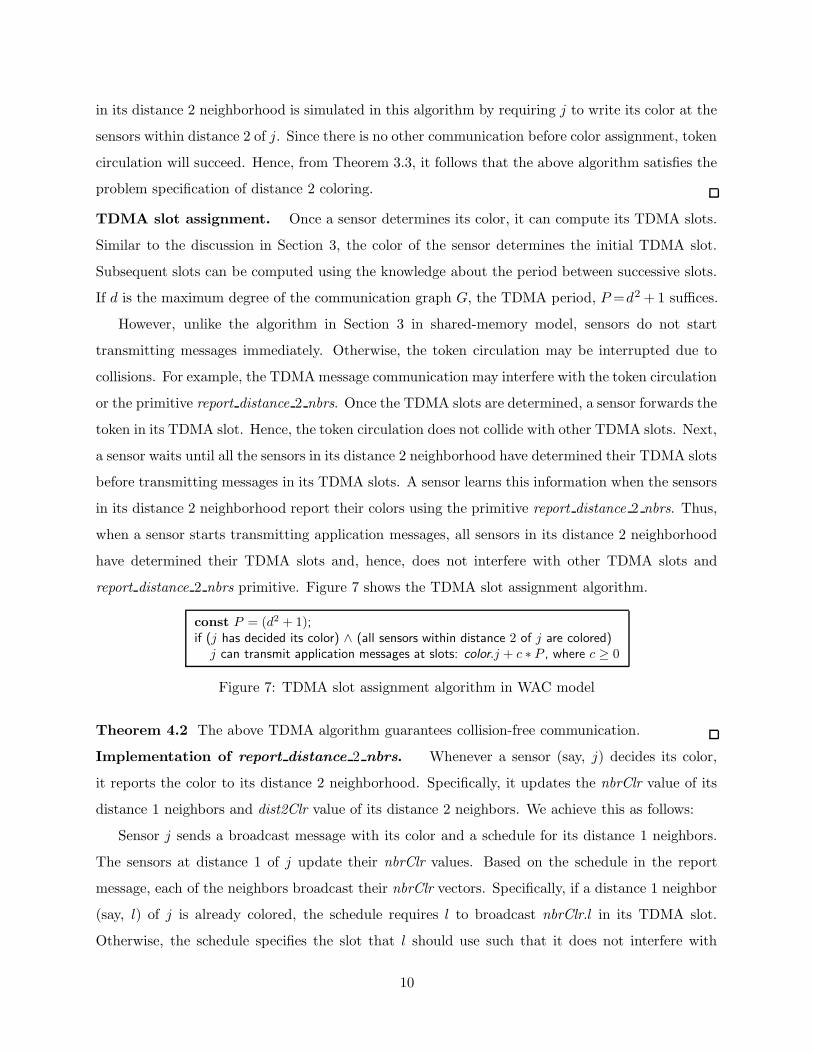
TDMA slot assignment. Once a sensor determines its color, it can compute its TDMA slots.

Similar to the discussion in Section 3, the color of the sensor determines the initial TDMA slot.

Subsequent slots can be computed using the knowledge about the period between successive slots.

If d is the maximum degree of the communication graph G, the TDMA period, P =d2 + 1 suffices.

However, unlike the algorithm in Section 3 in shared-memory model, sensors do not start

transmitting messages immediately. Otherwise, the token circulation may be interrupted due to

collisions. For example, the TDMA message communication may interfere with the token circulation

or the primitive report distance 2 nbrs. Once the TDMA slots are determined, a sensor forwards the

token in its TDMA slot. Hence, the token circulation does not collide with other TDMA slots. Next,

a sensor waits until all the sensors in its distance 2 neighborhood have determined their TDMA slots

before transmitting messages in its TDMA slots. A sensor learns this information when the sensors

in its distance 2 neighborhood report their colors using the primitive report distance 2 nbrs. Thus,

when a sensor starts transmitting application messages, all sensors in its distance 2 neighborhood

have determined their TDMA slots and, hence, does not interfere with other TDMA slots and

report distance 2 nbrs primitive. Figure 7 shows the TDMA slot assignment algorithm.

const P = (d2 + 1);if (j has decided its color) ∧ (all sensors within distance 2 of j are colored)

j can transmit application messages at slots: color.j + c ∗ P , where c ≥ 0

Figure 7: TDMA slot assignment algorithm in WAC model

Theorem 4.2 The above TDMA algorithm guarantees collision-free communication.

Implementation of report distance 2 nbrs. Whenever a sensor (say, j) decides its color,

it reports the color to its distance 2 neighborhood. Specifically, it updates the nbrClr value of its

distance 1 neighbors and dist2Clr value of its distance 2 neighbors. We achieve this as follows:

Sensor j sends a broadcast message with its color and a schedule for its distance 1 neighbors.

The sensors at distance 1 of j update their nbrClr values. Based on the schedule in the report

message, each of the neighbors broadcast their nbrClr vectors. Specifically, if a distance 1 neighbor

(say, l) of j is already colored, the schedule requires l to broadcast nbrClr.l in its TDMA slot.

Otherwise, the schedule specifies the slot that l should use such that it does not interfere with

10

the slots already assigned to j’s distance 2 neighborhood. If there exists a sensor k such that

distanceG(l, k) ≤ 2, then k will not transmit in its TDMA slots, as l is not yet colored. Now, a

sensor (say, m) updates dist2Clr.m with 〈j, color.j〉 iff (m 6= j) ∧ (j 6∈ N.m). Thus, this schedule

guarantees collision-free update of color.j at sensors within distance 2 of j. Further, this primitive

requires at most d+1 update messages.

4.1 Computing the TDMA Period

In this section, we present the algorithm for computing the ideal TDMA period. Towards this

end, first, we note that when a sensor (say, j) starts transmitting application messages, it has

the knowledge about the colors assigned to sensors within distance 2 of j. Hence, j can compute

the maximum color assigned to the sensors in its distance 2 neighborhood. Specifically, MC.j =

max(color.j ∪ used.j), where used.j is the colors used in the distance 2 neighborhood of j.

Now, we use the token circulation algorithm to compute the maximum color used in the network.

Let token.MC denote the maximum color in the network. When the base station (i.e., r) initiates

token circulation, it sets token.MC =MC.r. Now, whenever a sensor (say, j) forwards the token,

it sets token.MC =max(token.MC,MC.j). It follows that when the base station receives the token

back, it will learn the maximum color used in the network. It can include this information when

it initiates the next token circulation (i.e., token.period= token.MC + 1) . As a result, the sensors

will learn the new TDMA period. When the base station initiates the subsequent token circulation,

the new TDMA period is used to determine the slots at which a sensor can send a message.

5 Adding Stabilization in WAC Model

In the algorithm presented in Section 4, if the sensors are assigned correct slots then validating

the slots is straightforward. Towards this end, we can use a simple diffusing computation to allow

sensors to report their colors to distance 2 neighborhood and ensure that the slots are consistent.

For simplicity of presentation, we assume that token circulation is used for revalidating TDMA

slots. Now, in the algorithm presented in Section 4, we observe that in the absence of any faults,

the token circulates the network successfully and, hence, slots are revalidated. However, in the

presence of faults, the network may contain no tokens or it may contain several tokens. The token

may be lost due to a variety of reasons, such as, (1) slots assigned to sensors are not collision-free,

(2) nbrClr values are corrupted, and/or (3) token message is corrupted over the radio. Or, due to

11

transient faults, there may be several tokens.

To obtain self-stabilization, we proceed as follows: first, we ensure that if the system contains

multiple tokens then it recovers to states where there is at most one token. Then, we ensure that

the system recovers to states where there is a unique token.

To deal with the case of multiple tokens, we ensure that any token in the network either returns

to the base station within a predetermined time or it is lost. Towards this end, we ensure that a

sensor forwards the token as soon as possible. To achieve this, whenever a sensor, say j, receives

the token, j updates its color at its neighbors in its TDMA slot. (This can be achieved within P

slots, where P is the TDMA period.) Furthermore, in the subsequent slots, (a) the neighbors relay

this information to distance 2 neighbors of j and (b) j forwards the token. (Both of these can be

achieved within P slots.) Observe that if the TDMA slots are valid then any token will return in

2 ∗P ∗ |Et| slots to the base station, where |Et| is number of edges traversed by the token, or it will

be lost (due to collision if TDMA slots are incorrect).

In order to revalidate the slots assigned to the sensors, the base station initiates a token circula-

tion once every token circulation period, Ptc slots. The value of Ptc is chosen such that it is at least

equal to the time taken for token circulation (i.e., Ptc ≥ 2 ∗ P ∗ |Et|). Thus, when the base station

(i.e., r) initiates a token circulation, it expects to receive the token back within Ptc. Towards this

end, the base station sets a timeout for Ptc duration whenever it forwards the token. Now, if the

base station sends a token at time t and it does not send any additional token before time t + Ptc

then all tokens in the network at time t will return to the base station before time t + Ptc or they

will be lost. Hence, when the timeout expires, there is no token in the network. If the base station

has received a token before the timeout expires, it recirculates the token to revalidate TDMA slots.

Otherwise (i.e., the base station has received no token before the timeout expires), it concludes

that the token is lost in the network. Similarly, whenever a sensor (say, j 6= r) forwards the token,

it expects to receive the token in the subsequent token circulation round within Ptc. Otherwise, it

sets the color values in nbrClr.j and dist2Clr.j to undefined. And, stops transmitting in its current

TDMA slots until it recomputes color.j and the sensors in its distance 2 neighborhood report their

color values. Therefore, at most one token resides in the network at any instant. Thus, we have

Lemma 5.1 For any system configuration, if the base station initiates a token circulation at time

t and does not initiate additional token circulation before time t + Ptc then no sensor other than

the base station has a token at time t + Ptc.

Now, if the token is lost in the network, the base station initiates a recovery by sending a recovery

12

token. Before the base station sends the recovery token, it waits until the sensors in its distance 3

neighborhood have stopped transmitting. This is to ensure that the primitive report distance 2 nbrs

can update the distance 2 neighbors of the base station successfully. Let Trt be the time required

for sensors in the distance 3 neighborhood of the base station to stop transmitting. Specifically,

the value of Trt should be chosen such that the sensors within distance 3 of the base station can

detect the loss of the token within this interval. Although, the actual value of Trt depends on the

algorithm used for token circulation, it is bounded by Ptc. After waiting for Trt amount of time,

the base station recomputes its color. Further, it reports its color to the sensors within distance 2

of it. As mentioned in Section 4, the primitive report distance 2 nbrs ensures collision-free update

since the sensors within distance 2 have stopped. Then, it forwards the recovery token.

Now, when a sensor (say, j) receives the recovery token, similar to the base station, it waits

until the sensors in the distance 3 neighborhood of j have stopped transmitting. Then, j follows

the algorithm in Section 4 to recompute its color. Once j decides its color, it uses the primitive

report distance 2 nbrs to update the sensors within distance 2 of j with color.j. Thus, we have

Lemma 5.2 Whenever a sensor (say, j) forwards the recovery token, sensors within distance 2 of

j are updated with color.j without collision.

Once a sensor recomputes its color, it can determine its TDMA slots using the algorithm in

Section 4. And, the sensor can start using the TDMA slots when the sensors in its distance 2

neighborhood are colored. Thus, we have

Theorem 5.3 With the above modification, starting from arbitrary initial states, the TDMA

algorithm in WAC model recovers to states from where collision-free communication among sensors

is restored.

Time complexity for recovery. Based on the above discussion, the value of Trt depends on

the algorithm used for token circulation. Suppose Trt =Ptc, i.e., the base station waits for one token

circulation period before forwarding the recovery token. Now, when the base station forwards the

recovery token, all the sensors in the network would have stopped transmitting. Further, whenever

a sensor receives the token, it can report its color without waiting for additional time. To compute

the time for recovery, observe that it takes (a) at most one token circulation time (i.e., Ptc) for

the base station to detect token loss, (b) one token circulation for the sensors to stop and wait

for recovery, and (c) at most one token circulation for the network to resume normal operation.

Thus, the time required for the network to self-stabilize is at most 2∗Ptc+ time taken for resuming

normal operation. Since the time taken for resuming normal operation is bounded by Ptc, the time

13

required for recovery is bounded by 3 ∗ Ptc.

We expect that depending on the token circulation algorithm, the recovery time can be reduced.

However, the issue of optimizing the recovery time is outside the scope of this paper. We refer the

reader to Section 7 for a discussion on how small perturbations can be recovered locally.

Optimizations for token circulation and recovery. Whenever the token is lost, recovery is

initiated by the base station. However, it is possible that the slots are still collision-free. This could

happen if the token is lost due to message corruption or synchronization errors. To deal with this

problem, the base station can choose not to initiate recovery as soon as the token is lost. Rather,

it can initiate recovery only if it misses the token for a threshold number of consecutive attempts.

Additionally, to ensure that the token is not lost due to message corruption, whenever a sensor

(say, j) forwards the token, it expects its successor (say, k ∈ N.j) to forward the token within a

certain interval. If j fails to receive such implicit acknowledgment from k, j retransmits the token

(in its TDMA slots) a threshold number of times. If a sensor receives duplicate tokens, it ignores

such messages. With this modification, the reliability of token circulation can be improved.

Optimizations for controlled topology changes. In our TDMA algorithm, addition/removal

of sensors do not affect the normal operation of the network. Let us first consider the removal/failure

of sensors. Whenever a sensor is removed or fails, the TDMA slots assigned to other sensors are still

collision-free and, hence, normal operation of the network is not interrupted. However, the slots

assigned to the removed/failed sensor are wasted. We refer the reader to Section 6 for a discussion

on how the sensors can reclaim these slots.

Suppose a sensor (say, q) is added to the network such that the assumption about the maximum

degree is not violated. Towards this end, we require that whenever a sensor forwards the token, it

includes its color and the colors assigned to its distance 1 neighbors. Before q joins the network and

starts transmitting application messages, we require q to learn the colors assigned to the sensors

within its distance 2 neighborhood. One way to achieve this is by listening to token circulation

of its distance 1 neighbors. Once q learns the colors assigned to sensors within distance 2, it can

choose its color. Thus, q can determine the TDMA slots that it can use. Now, when q sends a

message, its neighbors learn the presence of q and include it in the subsequent token circulations.

With this approach, if two or more sensors are added simultaneously then these new sensors

may choose conflicting colors and, hence, collisions may occur. Since the TDMA algorithm is

self-stabilizing, the network self-stabilizes to states where the colors assigned to all the sensors are

collision-free. Thus, new sensors can be added to the network. However, if adding new sensors

14

violates the assumption about the maximum degree of the communication graph, slots may not be

assigned to the sensors and/or collisions may occur.

6 Extension: Local Negotiation Based Bandwidth Reservation

The algorithm in Section 5 allocates uniform bandwidth to all sensors. In this section, we consider

an extension where a sensor can request for additional bandwidth, if available. This extension is

based on the traditional mutual exclusion algorithms and it utilizes the fact that there is time

synchronization and reliable timely delivery provided by TDMA.

In our TDMA algorithm, each sensor is aware of the slots used by the sensors in its distance 2

neighborhood. Hence, a sensor can determine the unused slots and if necessary request for the same.

Whenever a sensor (say, j) requires additional bandwidth, it broadcasts a request slot message in its

TDMA slot. The message includes the slot requested by j and the time when j made the request.

Since the message is broadcast, all distance 1 neighbors of j will receive the message. The distance

1 neighbors of j rebroadcast the message immediately to their neighbors in their earliest TDMA

slots. If two or more request slot messages are received before the communication slot assigned to

a sensor, these messages are grouped and sent as a single request message.

Now, we show that if j transmitted its request in timeslot xj and it did not receive any other

request with timestamp ts such that ts < xj + P then j can access the requested timeslot without

collisions. Towards this end, observe that if j transmits at slot xj, all distance 1 neighbors of

j can transmit at least once before j’s next slot, xj + P , where P is the TDMA period. Thus,

if xj is the slot when j requests unused slots, this request message is received by sensors in its

distance 2 neighborhood within slot xj + P . Likewise, if sensor l requests for the same slot such

that distanceG(j, l) ≤ 2, j will learn about l’s request within time P of the request. Hence, if j does

not receive a request with earlier timestamp before xj +P then j can use its requested slot without

collisions. Furthermore, if j and l request for same slot then only one of them would succeed as the

slots in which they request are different (due to collision-freedom of TDMA slots). Additionally,

lease mechanisms [18] could be used to avoid starvation, where a sensor is required to renew the

additional slots within a certain period of time.

Thus, sensors can request for unused slots when necessary using a simple local negotiation proto-

col. Further, when a sensor requests unused slots, at most d + 1 request messages are transmitted,

where d is the maximum degree of the communication graph. And, the sensor can determine

whether or not it is allowed to use the requested slots within P slots.

15

7 Discussion and Related Work

In this section, we discuss some of the questions raised by this work and the related work.

Scalability. One of the questions about the transformation is scalability. While the algorithm

uses a token circulation approach for assigning initial colors (or recalculating them in the context

of stabilization), we note that the algorithm provides acceptable performance in a typical scenario

where sensor networks are deployed. Furthermore, to our knowledge, this is the first algorithm that

provides deterministic self-stabilizing TDMA service.

To illustrate the issue of scalability, we consider a network with 100 MICA-2 sensors. (Typically,

networks with more than 100 sensors will be organized in sections to ensure that the path to a base

station is within acceptable limits [5]. Then, our algorithm can be used independently for each

section.) If such sensors are arranged in a 10x10 communication grid then five colors suffice [10].

The token circulation time (Ptc) in such networks is 0.99 minutes (where the timeslot interval is

30ms = the time required to transmit one message in MICA-2 motes) and, hence the recovery time is

3∗Ptc =2.97 minutes. Thus, the time required for the network to self-stabilize is small. Additionally,

we expect that the number of colors required to obtain distance 2 coloring is small for random

deployments. This is due to the following reasons: (1) the maximum degree of a communication

graph is expected to be small, and (2) sensors execute as part of an energy conservation scheme and,

hence, the number of sensors that cover a particular coordinate in the target field is limited [19].

Therefore, our algorithm provides acceptable performance in such deployments.

Local recovery. It is possible to extend our algorithm so that sensors can locally correct

the corrupted slots when only a small number of sensors is corrupted. For example, if a sensor

learns that its color overlaps with its neighbor within distance 2, it can change its color locally.

Alternatively, if only a small set of sensors are corrupted then we could combine our algorithm with

that in [8]. Specifically, whenever a sensor detects that the slots assigned to a sensor are corrupted,

initially, it could use the algorithm in [8] to locally correct the slots assigned to the sensor. Thus,

for the case where only a small subset of sensors are corrupted, the slots will be quickly restored.

However, if it fails to assign slots in a fixed interval then the recovery token from the base station will

restore the slots. Local recovery is especially useful if the base station tries multiple tokens before

initiating recovery. Specifically, in this case, small perturbations are corrected locally. However, if

the corruption is excessive then our algorithm will ensure recovery in a deterministic interval.

Edge coloring vs. vertex coloring. Edge coloring is the problem of assigning time slots

16

to each edge of the network. Formally, the problem of edge coloring is stated as follows: Let

f(a, b) be the color assigned to edge (a, b); then ∀(x, y) : (f(x, y) 6∈ ({f(j, x)|j is a neighbor of

x} ∪ {f(l, y), f(y, l)|(x 6= l) ∧ (l is a neighbor of y)}). Now, a sensor (say, x) can send messages at

slots ∃y : y is a neighbor of x : f(x, y). Moreover, x can send messages at slots f(x, y) + c ∗ K,

where c ≥ 0 and K (the TDMA period) is the number of colors used in the network. Based on

the color assignments, whenever x sends a message in the slot f(x, y) + c ∗ K, sensor y receives

the message successfully (although it may cause collision elsewhere). Hence, in order to broadcast

a given message m with this approach, a sensor has to transmit m up to d times, where d is

the maximum degree of the communication graph. Edge coloring is thus not energy-efficient. By

contrast, in this paper, we propose vertex coloring, where a sensor has to transmit only once in

order to broadcast a message to all its neighbors.

Related work. Related work that deals with collision-free communication protocols for sensor

networks include [8–10, 20, 21]. In [8], Herman and Tixeuil propose a randomized TDMA slot

assignment algorithm where a probabilistic fast clustering technique is used. In their algorithm,

first, a maximal independent set is computed. This set identifies the leaders that are responsible

for obtaining distance 2 coloring. Further, addition/removal of nodes in their algorithm can cause

local collisions (and the effects are contained within distance 3 neighborhood). By contrast, our

approach uses a deterministic algorithm to assign time slots. Moreover, addition/removal of sensors

do not affect TDMA as long as the maximum degree assumption is not violated.

In [9], Busch et al propose a randomized TDMA algorithm for sensor networks. In their ap-

proach, initially, a randomized algorithm is used to determine the slots. Later, the sensors enter

another phase where the TDMA period is reduced. Both the phases of the algorithm are self-

stabilizing and are interleaved. By contrast, we propose a deterministic TDMA solution, where the

sensors identify their time slots without any collisions.

In [10], Kulkarni and Arumugam propose a self-stabilizing TDMA algorithm where the topology

is known and cannot change. However, in our algorithm, we allow addition/removal of sensors.

Additionally, in our solution, we require that the sensors are only aware of their local neighborhood.

In [20], Sohrabi and Pottie propose a network self-organization protocol, where nodes identify

the presence of other nodes and form a multi-hop network. In [21], Heinzelman et al propose a

clustering algorithm. In both these papers, initially, nodes are in random access mode and TDMA

slots are assigned during network organization. By contrast, in our solution, we use a deterministic

algorithm to assign time slots. Moreover, our algorithm is self-stabilizing.

17

8 Conclusion

In this paper, we presented a self-stabilizing, deterministic time division multiple access (TDMA)

algorithm for sensor networks. Such algorithms are desirable in sensor networks for energy manage-

ment, as TDMA allows a sensor to reduce the amount of idle listening. Moreover, as discussed in [2],

such algorithms suffice in transforming programs written in read/write model or shared-memory

model into programs in write all with collision (WAC) model.

We first discussed our algorithm in shared-memory model. In this algorithm, we systemati-

cally reused existing graph traversal algorithms (e.g., [11–13]) to obtain distance 2 coloring. We

then showed that this algorithm is self-stabilizing. Once distance 2 coloring is obtained, the sen-

sors are allowed to compute their slots using the knowledge about the maximum degree of the

communication graph. We showed that the TDMA slot assignment is also self-stabilizing.

Next, we transformed the TDMA algorithm in shared-memory model into WAC model. We

showed that the network self-stabilizes within a deterministic interval. Also, we showed that there

is a tradeoff between the frequency with which slots assigned to the sensors are revalidated and the

recovery time. Moreover, with this scheme, we showed that controlled addition/removal of sensors

are possible provided they do not violate the maximum degree assumption.

While we expect that the degree of each sensor to be small, the number of colors used in our

algorithm is at most d times the optimal, where d is the maximum degree of the communication

graph. Also, in this paper, we showed that the TDMA period and the bandwidth utilization of

sensors can be improved further. Towards this end, we discussed an approach where the sensors are

allowed to reduce the TDMA period depending on the maximum color assigned in the distance 2

neighborhood of all sensors. Furthermore, we presented an extension where sensors can request for

additional bandwidth whenever necessary. With this scheme, whenever a sensor requires additional

bandwidth, we showed that at most d + 1 messages are transmitted and it learns whether or not it

is allowed to use the requested bandwidth within P slots.

There are several possible extensions to this work. We are currently working on extending

this algorithm to determine the ideal TDMA period in the neighborhood of each sensor. With

this extension, we expect that the bandwidth utilization can be improved even further. Another

extension is to adapt the algorithm presented in this paper to assign more bandwidth to sensors

closer to the base station as they often act as a bottleneck in sensor networks.

18

References

[1] P. Dutta, M. Grimmer, A. Arora, S. Bibyk, and D. Culler. Design of a wireless sensor network platform fordetecting rare, random, and ephemeral events. In Proceedings of the Conference on Information Processing inSensor Networks (IPSN), SPOTS track, April 2005.

[2] S. S. Kulkarni and M. Arumugam. Transformations for write-all-with-collision model. Computer Communications(Elsevier), Special Issue on Dependable Wireless Sensor Networks, 2005, to appear. Also, appeared in theProceedings of the International Conference on Principles of Distributed Systems (OPODIS), 2003.

[3] E. W. Dijkstra. Self-stabilizing systems in spite of distributed control. Communications of the ACM, 1974.

[4] S. Dolev. Self-Stabilization. The MIT Press, 2000.

[5] The Ohio State University team. ExScal: Extreme scaling in sensor networks for target detection, classification,tracking. DARPA demonstration, December 2004, Avon Park, FL. http://www.cse.ohio-state.edu/exscal.

[6] A. Arora, P. Dutta, S. Bapat, V. Kulathumani, H. Zhang, V. Naik, V. Mittal, H. Cao, M. Demirbas, M. Gouda,Y-R. Choi, T. Herman, S. S. Kulkarni, U. Arumugam, M. Nesterenko, A. Vora, and M. Miyashita. A line in thesand: A wireless sensor network for target detection, classification, and tracking. Computer Networks (Elsevier),46(5):605–634, December 2004.

[7] A. Mairwaring, J. Polastre, R. Szewczyk, D. Culler, and J. Anderson. Wireless sensor networks for habitatmonitoring. International Workshop On Wireless Sensor Networks and Applications, 2002.

[8] T. Herman and S. Tixeuil. A distributed TDMA slot assignment algorithm for wireless sensor networks. Work-shop on Algorithmic Aspects of Wireless Sensor Networks, 2004.

[9] C. Busch, M. M-Ismail, F. Sivrikaya, and B. Yener. Contention-free MAC protocols for wireless sensor networks.In Proceedings of the 18th Annual Conference on Distributed Computing (DISC), 2004.

[10] S. S. Kulkarni and M. Arumugam. SS-TDMA: A self-stabilizing MAC for sensor networks. In Sensor Net-work Operations. IEEE Press, 2005, to appear. Available at: http://www.cse.msu.edu/~arumugam/research/

papers/ieee-sn-operations05.

[11] C. Johnen, G. Alari, J. Beauquier, and A. K. Datta. Self-stabilizing depth-first token passing on rooted networks.In Proceedings of the 11th International Workshop on Distributed Algorithms (WDAG), pages 260–274, 1997.

[12] F. Petit and V. Villain. Color optimal self-stabilizing depth-first token circulation. In Proceedings of theInternational Symposium on Parallel Architectures, Algorithms, and Networks (ISPAN), 1997.

[13] F. Petit. Fast self-stabilizing depth-first token circulation. In Proceedings of the Workshop on Self-StabilizingSystems, Springer, LNCS:2194:200–215, 2001.

[14] T. Herman. NestArch: Prototype time synchronization service. NEST Challenge Architecture. Available at:http://www.ai.mit.edu/people/sombrero/nestwiki/index/ComponentTimeSync, January 2003.

[15] E. L. Lloyd and S. Ramanathan. On the complexity of distance-2 coloring. In Proceedings of the FourthInternational Conference on Computing and Information, 1992.

[16] S. Ramanathan and E. L. Lloyd. Scheduling algorithms for multihop radio networks. IEEE/ACM Transactionson Networking, 1(2):166–177, April 1993.

[17] S. O. Krumke, M. V. Marathe, and S. S. Ravi. Models and approximation algorithms for channel assignment inradio networks. Wireless networks, 7(6):575–584, November 2001.

[18] A. S. Tanenbaum. Computer Networks. Prentice Hall, 4th edition, March 2003.

[19] D. Tian and N. D. Georganas. A coverage-preserving node scheduling scheme for large wireless sensor networks.In Proceedings of the ACM International Workshop on Wireless Sensor Networks and Applications, 2002.

[20] K. Sohrabi and G. J. Pottie. Performance of a novel self-organization protocol for wireless ad-hoc sensor networks.In Proceedings of the IEEE Vehicular Technology Conference, pages 1222–1226, 1999.

[21] W. B. Heinzelman, A. P. Chandrakasan, and H. Balakrishnan. An application-specific protocol architecture forwireless microsensor networks. IEEE Transactions on Wireless Communications, 1(4):660–670, October 2002.

19

Appendix

A Proofs

In this section, we present the proofs of the theorems in Section 3.

Lemma 3.1 If d is the maximum degree of a graph then d2 + 1 colors are sufficient to obtaindistance 2 coloring.Proof. Based on the assumption about degree, given any vertex v, there exists at most d distance1 neighbors, d(d − 1) distance 2 neighbors. Thus, at most d2 vertices are within distance 2 of v.Now, we can arrange the vertices in some order and allow them to choose a color in such a way thatthe choice does not conflict with vertices that are considered earlier and within distance 2. When avertex is about to choose a color, at most d2 colors could be in its distance 2 neighborhood. Thus,a vertex can choose a color such that it does not overlap with the colors assigned to vertices in itsdistance 2 neighborhood.

Theorem 3.4 Starting from arbitrary initial states, the above algorithm recovers to states fromwhere the problem specification of distance 2 coloring is satisfied.Proof. Based on the assumption in Section 3.1, the token circulation layer is self-stabilizing.The TDMA layer preserves the stabilization property of the token circulation layer since it even-tually allows a sensor to forward the token. Thus, starting from arbitrary initial states, the tokencirculation algorithm self-stabilizes to states where only one token is present in the network. In thecirculation of the token after stabilization, we show that the following conditions are satisfied.

• Given any sensor va that is visited by the token, color of va does not conflict with sensorsthat are within distance 2 of va and have been visited.

• Given any sensor va that is visited by the token, color of va is correctly captured in all itsneighbors.

Let v1, v2, . . . , vx be the path taken by the token after stabilization. It is straightforward to seethat the above conditions are satisfied when the token is sent by v1. Furthermore, based on thealgorithm, these conditions are preserved when the token is passed. When the token circulation iscomplete, based on the above conditions, it follows that the specification of distance 2 coloring issatisfied and the colors will be unchanged in subsequent token circulations.

Theorem 3.5 The TDMA slots assigned to the sensors by the above algorithm are collision-free.Proof. Consider two distinct sensors j and k such that the distance between j and k in thecommunication graph G is at most 2. The time slots assigned to j and k are color.j + c ∗ P andcolor.k + c ∗ P respectively, where c is an integer and P = (d2 + 1). Suppose a collision occurswhen j and k transmit a message at slot color.j + c1 ∗ P and color.k + c2 ∗ P respectively, wherec1, c2 > 0. In other words, color.j + c1 ∗ P = color.k + c2 ∗ P . From Theorem 3.3, we know thatcolor.j 6= color.k. Therefore, collision will occur iff |color.j − color.k| is a multiple of P . However,since the distance between j and k is at most 2, |color.j − color.k| is at most d2 (less than P ). Inother words, |color.j − color.k| ≤ d2 < P . Hence, if j and k transmit at the same time, then thedistance between them is greater than 2. This is a contradiction. Thus, collisions cannot occur inthis algorithm.

20