self-stabilizing robot formations over unreliable networks

17

Self-Stabilizing Robot Formations overUnreliable Networks

SETH GILBERT

Ecole Polytechnique Federale, Lausanne

NANCY LYNCH

Massachusetts Institute of Technology

SAYAN MITRA

University of Illinois at Urbana-Champaign

and

TINA NOLTE

Massachusetts Institute of Technology

We describe how a set of mobile robots can arrange themselves on any specified curve on theplane in the presence of dynamic changes both in the underlying ad hoc network and in theset of participating robots. Our strategy is for the mobile robots to implement a self-stabilizingvirtual layer consisting of mobile client nodes, stationary Virtual Nodes (VNs), and local broad-cast communication. The VNs are associated with predetermined regions in the plane and co-ordinate among themselves to distribute the client nodes relatively uniformly among the VNs’regions. Each VN directs its local client nodes to align themselves on the local portion of thetarget curve. The resulting motion coordination protocol is self-stabilizing, in that each robotcan begin the execution in any arbitrary state and at any arbitrary location in the plane. Inaddition, self-stabilization ensures that the robots can adapt to changes in the desired targetformation.

Categories and Subject Descriptors: F.1.2 [Computation by Abstract Devices]: Modes of Compu-tation—Interactive and reactive computation; H.3.4 [Information Storage and Retrieval]: Sys-tems and Software—Distributed systems; C.2.4 [Computer-Communication Networks]: Dis-tributed Systems—Distributed applications

General Terms: Algorithms, Reliability

This work was funded in part by NSF CSR program (Embedded & Hybrid systems area) undergrant NSF CNS-0614993 for S. Mitra.Authors’ addresses: S. Gilbert, Laboratory for Distributed Programming, Ecole PolytechniqueFederale, Lausanne; email: [email protected]; N. Lynch, Department of Electrical Engineeringand Computer Science, MIT; email: [email protected]; S. Mitra, Department of Electrical andComputer Engineering, University of Illinois at Urbana-Champaign; email: [email protected];T. Nolte, Department of Electrical Engineering and Computer Science, MIT; email: [email protected] to make digital or hard copies of part or all of this work for personal or classroom useis granted without fee provided that copies are not made or distributed for profit or commercialadvantage and that copies show this notice on the first page or initial screen of a display alongwith the full citation. Copyrights for components of this work owned by others than ACM must behonored. Abstracting with credit is permitted. To copy otherwise, to republish, to post on servers,to redistribute to lists, or to use any component of this work in other works requires prior specificpermission and/or a fee. Permissions may be requested from Publications Dept., ACM, Inc., 2 PennPlaza, Suite 701, New York, NY 10121-0701 USA, fax +1 (212) 869-0481, or [email protected]© 2009 ACM 1556-4665/2009/07-ART17 $10.00DOI 10.1145/1552297.1552300 http://doi.acm.org/10.1145/1552297.1552300

ACM Transactions on Autonomous and Adaptive Systems, Vol. 4, No. 3, Article 17, Publication date: July 2009.

17:2 • S. Gilbert et al.

Additional Key Words and Phrases: Formal methods, cooperative mobile robotics, distributed al-gorithms, pattern formation, self-stabilization, replicated state machines

ACM Reference Format:Gilbert, S., Lynch, N., Mitra, S., and Nolte, T. 2009. Self-Stabilizing robot formations over unreli-able networks. ACM Trans. Autonom. Adapt. Syst. 4, 3, Article 17 (July 2009), 29 pages.DOI = 10.1145/1552297.1552300 http://doi.acm.org/10.1145/1552297.1552300

1. INTRODUCTION

In this article, we study the problem of coordinating the behavior of autonomousmobile robots, even as robots join and leave the system. Consider, for example, asystem of firefighting robots deployed throughout forests and other arid wilder-ness areas. Significant levels of coordination are required in order to combat thefire: to prevent the fire from spreading, it has to be surrounded; to put out thefire, firefighters need to create “firebreaks” and spray water; they need to directthe actions of (potentially autonomous) helicopters carrying water. All this hasto be achieved while the set of participating agents is changing and despiteunreliable (often, wireless) communication between agents. Similar scenariosarise in a variety of contexts, including search and rescue, emergency disasterresponse, remote surveillance, and military engagement, among many others.In fact, autonomous coordination has long been a central problem in mobilerobotics.

We focus on a generic coordination problem that, we believe, captures manyof the complexities associated with coordination in real-world scenarios. Weassume that the mobile robots are deployed in a large two-dimensional plane,and that they can coordinate their actions by local communication using wire-less radios. The robots must arrange themselves to form a particular pattern,specifically, a continuous curve drawn in the plane. The robots must spreadthemselves uniformly along this curve. In the firefighting example describedbefore, this curve might form the perimeter of the fire.

These types of coordination problems can be quite challenging due to thedynamic and unpredictable environment that is inherent to wireless ad hocnetworks. Robots may be continuously joining and leaving the system, andthey may fail unpredictably. In addition, wireless communication is notoriouslyunreliable due to collisions, contention, and various wireless interference.

Virtual Infrastructure. Recently, virtual infrastructure has been proposedas a new tool for building reliable and robust applications in unreliable and un-predictable wireless ad hoc networks (e.g., Dolev et al. [2005, 2003]; Chockleret al. [2008]). The basic principle motivating virtual infrastructure is that manyof the challenges resulting from dynamic networks could be obviated if therewere reliable network infrastructures available. We believe that coordinatingmobile robots is exactly one of those problems. Unfortunately, in many con-texts, such infrastructure is unavailable. The virtual infrastructure abstrac-tion emulates real reliable infrastructure in ad hoc networks. Thus, it providesa programming abstraction that assumes reliable infrastructure, and thus sim-plifies the problem of developing applications. It has already been observed that


Self-Stabilizing Robot Formations over Unreliable Networks • 17:3

virtual infrastructure simplifies several problems in wireless ad hoc networks,including distributed shared memory implementations [Dolev et al. 2003],tracking mobile devices [Nolte and Lynch 2007b], geographic routing [Dolevet al. 2005b], and point-to-point routing [Dolev et al. 2004].

In this article, we rely on a virtual infrastructure known as the VirtualStationary Automata Layer (VSA layer) [Dolev et al. 2005a; Nolte and Lynch2007a]. In the VSA layer, each robot is modeled as a client; clients interactwith Virtual Stationary Automata (VSAs) via a (virtual) communication service.VSAs are distributed throughout the world, each assigned to its own uniqueregion. VSAs remain always at a known and predictable location, and they areless likely to fail than any individual mobile robot. Notice that the VSAs do notactually exist in the real world; they are emulated by the underlying mobilerobots. It is for this reason that a VSA is more reliable: It is as reliable as theentire collection of mobile nodes that are participating in its emulation.

In fact, we believe that the VSA layer is particularly suitable for solvingproblems such as motion coordination due to the failure properties of VSAs.In many ways, VSAs and mobile robots have a fate-sharing relationship: AVSA responsible for some specific region fails only when all the robots in itsregion fail or leave. Thus, as long as there are robots to coordinate, the VSA isguaranteed to remain alive. Conversely, whenever the VSA is failed, there areno robots alive or nearby that rely on the VSA. Thus from the perspective ofthe mobile robots, the VSAs appear completely reliable.

We do not address here the problem of implementing virtual infrastructure;instead, we refer the reader to Dolev et al. [2005a], Nolte and Lynch [2007a],and Nolte [2008]. In these articles, we show how to emulate VSAs using mo-bile, wireless devices much like the mobile robots discussed in this article. Thewireless devices have access to a synchronized time service, and a localizationservice (such as a GPS device), and they communicate via reliable and timelyradio broadcasts. In Section 4.2 we provide a brief overview of these require-ments, and of the protocol for implementing virtual infrastructure.

Coordinating Mobile Robots. Our main contribution is a technique for usingthe VSA layer to implement a reliable and robust protocol for coordinatingmobile robots. The key simplifying fact of the VSA layer is that reliable VSAsare distributed evenly throughout the world. Thus, each VSA is responsiblefor organizing the mobile robots in some region of the world. As the executionprogresses, each VSA directs the robots in its region as to how they shouldmove. There are two further technical issues that arise in our protocol: Howdoes the VSA collect the information that it needs (and how much informationdoes it need), and how, given only limited information, does the VSA direct themobile robots in order to ensure a good distribution of robots along the curve?In brief, we address these issues as follows.

In order to determine where each robot should go, the VSA needs to collectinformation about the current distribution of the robots. Each robot in a regionnotifies the responsible VSA of its presence, and, in addition, the VSAs exchangeinformation with their neighboring VSAs. Thus, each VSA maintains a localview of the number of robots it and its neighbors are responsible for. Of note,



the VSA only collects local information, that is, the distribution of robots in itsown and neighboring regions. It does not, for example, collect information aboutthe location of every robot, as this would take prohibitively long (and might noteven be possible, if the network induced by the robots is initially partitioned).

Using this local information about robot distribution, the VSA decides howmany robots to keep in its own region, and how many to distribute to its neigh-bors. By carefully reallocating robots, the VSAs cause the robots to diffusethroughout the network. The diffusion process is biased by the length of thecurve in each region to ensure that the concentration of robots reflects the needsof each VSA. Once the robots have diffused throughout the network, each VSAassigns the robots to locations on the curve.

Self-Stabilization. In order that the robot coordination be truly robust, ourcoordination protocol is self-stabilizing. In general, a self-stabilizing system isone which regains normal functionality and behavior sometime after distur-bances, such as when there are node failures and message losses cease.

In our case, this means that each robot can begin in an arbitrary state, inan arbitrary location in the network, and with an arbitrary view of the world.Even so, the distribution of the robots will still converge to the specified curve.When combined with a self-stabilizing implementation of the VSA layer, asis presented in Dolev et al. [2005a] and Nolte and Lynch [2007a], we endup with entirely self-stabilizing solution for the problem of autonomous robotcoordination.

We believe that self-stabilization is particularly important in the context ofwireless networks. Most of the time, wireless communication works reasonablywell. Most of the time, mobile robots act as expected. Our algorithms (and thosefor implementing virtual infrastructure) rely on this common case behavior:Communication is reliable, mobile robots move as directed, GPS devices returncorrect locations, etc.

And yet, in the real world, mobile robots are not perfectly reliable. Sometimesthey fail to move exactly as expected, due to minor errors in actuating theirmotors, bad sensor readings, or perhaps due to incorrectly detecting (or notdetecting) obstacles that must be avoided.1 Sometimes GPS devices return anincorrect location, or cannot acquire a sufficient number of satellites to returngood localization information. Sometimes there is electromagnetic interferencethat disrupts communication. Sometimes wireless messages are lost due totoo much contention, that is, too many different applications attempting tocommunicate on a limited bandwidth. There are a wide variety of problems thatcan occur in a deployment of mobile robots, and a wide variety of disruptionsthat can interfere with wireless communication. All of these challenges result indeviations from the common case setting for which our algorithms are designed.

Thus, there are clearly two options available for coping with this situation.One option is to design algorithms that can directly handle these challenges,

1In fact, much of the prior work on fault-tolerant motion coordination has focused on the problemsthat arise when the robots have faulty vision or a bad sense of direction. Unlike these prior articles,we allow the robots to coordinate via radio broadcasts. Thus, problems caused by faulty vision arelimited to disrupting the expected movement of the robots.



and yet still achieve the desired outcome. Pursuing this direction leads to al-gorithms that are immensely complicated. Moreover, it requires carefully enu-merating all the possible problems that might occur; any unexpected disruptioncan lead to a complete failure.

A second option, and the one that we pursue, is self-stabilization. A self-stabilizing algorithm can recover from all types of problems, as long as theerrors are temporary. In effect, a self-stabilizing algorithm requires only thatthe robots and the wireless communication work correctly most of the time. Inthis way, such protocols are a classic example of the paradigm, plan for the worst,expect the best. Despite occasional problems, the mobile robots will converge tothe desired formation.

Another advantage to self-stabilization is the capacity to cope with moredynamic coordination problems. In real-life scenarios, the required formationof the mobile nodes may change. In the firefighting example given earlier, asthe fire advances or retreats, the formation of firefighting robots must adapt. Aself-stabilizing algorithm can adapt to these changes, continually rearrangingthe robots along the newly chosen curve.

Proof Techniques. Analyzing self-stabilizing algorithm can be quite difficult,however, and another technical contribution of this article is the exemplifica-tion of a proof technique for showing self-stabilization of systems implementedusing virtual infrastructure. The proof technique has three parts. First, usinginvariant assertions and standard control theory results we show that fromany initial state, the application protocol in this case, the motion coordinationalgorithm converges to an acceptable state. Next, we show that the algorithmalways reaches a legal state even when it starts from some arbitrary state af-ter failures. From any legal state the algorithm gets to an acceptable state,provided there are no further failures. Finally, using a simulation relation weshow that the preceding set of legal states is in fact equal to the set of reach-able states of the complete system: the coordination algorithm composed withthe VSA layer. It has already been shown in Dolev et al. [2005a] and Nolteand Lynch [2007a] that the VSA layer itself is self-stabilizing. Thus, combiningthe stabilization of the VSA layer and the application protocol, we are able toconclude self-stabilization of the complete system.

Roadmap. The remainder of this article is organized as follows: In Section 2,we discuss some of the related work. In Section 3, we introduce the underlyingmathematical model, namely Timed I/O Automata (TIOA), used for specifyingthe VSA layer. We discuss how to transform a TIOA designed for a reliable net-work into a TIOA that executes in an unreliable system, and we define whatit means for a TIOA to be self-stabilizing. In Section 4 we present the overallVSA layer architecture, describing the behavior of each of the underlying com-ponents. We also briefly describe how to emulate the VSA layer in a wirelessnetwork. In Section 5 we begin by formally describing the motion coordina-tion problem and an algorithm that solves the problem of motion coordination.The algorithm is divided into two components: The first part (i.e., the clientcode) runs on the mobile robots and simply sends updates to the VSA, receives



responses from the VSAs, and then moves as directed. The second part (i.e., theserver code) runs on the VSAs, and is responsible for planning the motion ofthe mobile robots. In Section 6, we show that the algorithm is correct assumingthat the system begins in a good state. We show that, eventually, the mobilerobots are appropriately distributed through the world, and that they arrangethemselves evenly along the curve. In Section 7, we show that the algorithm isself-stabilizing. We define two legal sets of states, and argue that the systemconverges to first one, and then the second of these legal sets. We then arguethat this second set of legal states is a “reachable” state from an initial state ofthe system. We conclude in Section 8.

2. RELATED WORK

In the distributed computing literature, the idea of self-stabilization has beenproposed an important way of engineering fault tolerance in systems that are in-herently unreliable [Dolev 2000]. The idea of self-stabilization has been widelyemployed for designing resilient distributed systems over unreliable communi-cation and computing components (see Herman [1996] for a comprehensive listof applications).

The problem of motion coordination has been studied in a variety of con-texts, focusing on several different goals: flocking [Jadbabaie et al. 2003]; ren-dezvous [Ando et al. 1999; Lin et al. 2003; Martinez et al. 2005]; aggrega-tion [Gazi and Passino 2003]; and deployment and regional coverage [Corteset al. 2004]. Control theory literature contains several algorithms for achievingspatial patterns [Fax and Murray 2004; Clavaski et al. 2003; Blondel et al. 2005;Olfati-Saber et al. 2007]. These algorithms assume that the agents process in-formation and communicate synchronously, and hence, they are analyzed basedon differential or difference equation models of the system. Convergence of thisclass of algorithms over unreliable and delay-prone communication channelshas been studied recently in Chandy et al. [2008].

Geometric pattern formation with vision-based models for mobile robotshas been investigated in Suzuki and Yamashita [1999], Prencipe [2001,2000], Flocchini et al. [2001], Efrima and Peleg [2007], and Defago andKonagaya [2002]. In these weak models, the robots are oblivious, identical,anonymous, and often without memory of past actions. For the memorylessmodels, the algorithms for pattern formation are often automatically self-stabilizing. In Defago and Konagaya [2002] and Defago and Souissi [2008], forinstance, a self-stabilizing algorithm for forming a circle has been presented.These weak models have been used for characterizing the class of patternsthat can be formed and for studying the computational complexity of forma-tion algorithms, under different assumptions about the level of common knowl-edge amongst agents, such as knowledge of distance, direction, and coordi-nates [Suzuki and Yamashita 1999; Prencipe 2000].

We have previously presented a protocol for coordinating mobile devices us-ing virtual infrastructure in Lynch et al. [2005]. The article described how to im-plement a simple asynchronous virtual infrastructure, and proposed a protocolfor motion coordination. This earlier protocol relies on a weaker (i.e., untimed)



virtual layer (see Dolev et al. [2005a] and Nolte and Lynch [2007a]), while thecurrent one relies on a stronger (i.e., timed) virtual layer. As a result, our newcoordination protocol is somewhat simpler and more elegant than the previ-ous version. Moreover, the new protocol is self-stabilizing, which allows bothfor better fault tolerance and also the ability to tolerate dynamic changes inthe desired pattern of motion. Virtual infrastructure has also been consideredin Brown [2007] for collision prevention of airplanes.

3. PRELIMINARIES

In this work we mathematically model the the virtual infrastructure and allcomponents of our algorithms using the Timed Input/Output Automata (TIOA)framework. TIOA is a mathematical modeling framework for real-time, dis-tributed systems that interact with the physical world. Here we present keyconcepts of the framework and refer the reader to Kaynar et al. [2005] for fur-ther details.

3.1 Timed I/O Automata

A timed I/O automaton is a nondeterministic state transition system in whichthe state may change either: (a) instantaneously, by means of a discrete transi-tion, or (b) continuously over an interval of time, by following a trajectory. LetV be a set of variables. Each variable v ∈ V is associated with a type whichdefines the set of values v can take on. The set of valuations of V , that is, map-pings from V to values, is denoted by val (V ). Each variable may be discreteor continuous. Discrete variables are used to model protocol data structures,while continuous variables are used to model physical quantities such as time,position, and velocity.

The semi-infinite real line R≥0 is used to model time. A trajectory τ for aset V of variables maps a left-closed interval of R≥0 with left endpoint 0 toval (V ). It models evolution of values of the variables over a time interval. Thedomain of τ is denoted by τ.dom. We define τ.fstate �= τ (0). A trajectory is closedif τ.dom = [0, t] for some t ∈ R≥0, in which case we define τ.ltime �= t andτ.lstate �= τ (t).

Definition 3.1. A TIOA A = (X , Q , �, A, D, T ) consists of: (a) a set X ofvariables; (b) a nonempty set Q ⊆ val (X ) of states; (c) a nonempty set � ⊆ Qof start states; (d) a set A of actions partitioned into input, output, and internalactions I , O, and H; (e) a set D ⊆ Q × A× Q of discrete transitions. If (x, a, x′) ∈D, we often write vx

a→ x′. An action a ∈ A is said to be enabled at x iff x a→ x′

for some x′; and (f) a set T of trajectories for X that is closed under prefix, suffix,and concatenation.2

In addition, A must be input action and input trajectory enabled.3 We as-sume in this work that the values of discrete variables do not change duringtrajectories.

2See Kaynar et al. [2005, Chapters 3 and 4], for formal definitions of these closure properties.3See Kaynar et al. [2005, Chapter 64].



We denote the components X , Q , D, . . . of a TIOA A by XA, QA, DA, . . . ,respectively. For TIOA A1, we denote the components by X 1, Q1, D1, . . . .

Executions. An execution of A records the valuations of all variables andthe occurrences of all actions over a particular run. An execution fragment ofA is a finite or infinite sequence τ0a1τ1a2 · · · such that for every i, τi.lstate

ai+1→τi+1.fstate. An execution fragment is an execution if τ0.fstate ∈ �. The first stateof α, which we refer to as α.fstate, is τ0(0), and for a closed α (i.e., one that isfinite and whose last trajectory is closed), its last state, α.lstate, is the last stateof its last trajectory. The limit time of α, α.ltime, is defined to be

∑i τi.ltime. A

state x of A is said to be reachable if there exists a closed execution α of A suchthat α.lstate = x. The sets of executions and reachable states of A are denotedExecsA and ReachA. The set of execution fragments of A starting in states in anonempty set L is denoted by FragsL

A.A nonempty set of states L ⊆ QA is said to be a legal set for A if it is closed

under the transitions and closed trajectories of A; that is, a legal set satisfiesthe following: (1) If (x, a, x′) ∈ DA and x ∈ L, then x′ ∈ L, and (2) if τ ∈ TA, τ isclosed, and τ.fstate ∈ L then τ.lstate ∈ L.

Traces. Often we are interested in studying the externally visible behaviorof a TIOA A. We define the trace corresponding to a given execution α by remov-ing all internal actions, and replacing each trajectory τ with a representationof the time that elapses in τ . Thus, the trace of an execution α, denoted bytrace(α), has information about input/output actions and the duration of timethat elapses between the occurrence of successive input/output actions. The setof traces of A is defined as TracesA

�= {β | ∃α ∈ ExecsA, trace(α) = β}.

Implementation. Our proof techniques often rely on showing that any be-havior of a given TIOA A is externally indistinguishable from some behaviorof another TIOA B. This is formalized by the notion of implementation. TwoTIOAs are said to be comparable if their external interfaces are identical, thatis, they have the same input and output actions. Given two comparable TIOAsA and B, A is said to implement B, if TracesA ⊆ TracesB. The standard techniquefor proving that A implements B is to define a simulation relation R ⊆ QA× QBwhich satisfies the following: If xRy, then every one-step move of A from a statex simulates some execution fragment of B starting from y, in such a way that:(1) the corresponding final states are also related by R, and (2) the traces ofthe moves are identical (see Kaynar et al. [2005, Section 4.5] for the formaldefinition).

Composition. It is convenient to model a complex system such as our VSAlayer as a collection of TIOAs running in parallel and interacting through inputand output actions. A pair of TIOAs are said to be compatible if they do not sharevariables or output actions, and if no internal action of either is an action ofthe other. The composition of two compatible TIOAs A and B is another TIOAwhich is denoted by A‖B. Binary composition is easily extended to any finitenumber of automata.



3.2 Failure Transform for TIOAs

In this article, we will describe algorithms that are self-stabilizing even in theface of ongoing mobile robot failures and recoveries. In order to model failuresand recoveries, we introduce a general failure transformation of TIOAs. Thus,we can define a TIOA A in terms of its correct behavior, and then analyze thebehavior of Fail(A), which models the behavior of A in a failure-prone system.

A TIOA A is said to be is fail-transformable if it does not have the variablefailed, and it does not have actions fail or restart. If A is fail-transformable, thenthe transformed automaton Fail(A) is constructed fromA by adding the discretestate variable failed, a Boolean that indicates whether or not the machine isfailed, and two additional input actions, fail and restart. The states of Fail(A)are the states of A, together with a valuation of failed. The start states Fail(A)are the states in which failed is arbitrary, but if it is false, then the rest ofthe variables are set to values consistent with a start state of A. The discretetransitions of Fail(A) are derived from those of A as follows: (1) an ordinaryinput transition at a failed state leaves the state unchanged, (2) an ordinaryinput transition at a nonfailed state is the same as in A, (3) a fail action setsfailed to true, (4) if a restart action occurs at a failed state then failed is set tofalse and the other state variables are set to a start state of A; otherwise, itdoes not change the state.

The set of trajectories of Fail(A) is the union of two disjoint subsets, onefor each value of the failed variable. The subset for failed = false consists oftrajectories of A with the addition of the constant value for failed. In otherwords, while Fail(A) is not failed, its trajectories basically look like those of Awith the value of the failed variable remaining false throughout the trajectories.The subset for failed = true consists of trajectories of all possible lengths inwhich all variables are constant; that is, while Fail(A) is failed, its state remainsfrozen. Note that this does not constrain time from passing, since any constanttrajectory, of any length, is allowed.

Performing a failure transformation on the composition A‖B of two TIOAresults in a new TIOA whose executions projected to actions and variables ofFail(A) or Fail(B) are in fact executions of Fail(A) or Fail(B), respectively.

3.3 Self-Stabilization of TIOAs

A self-stabilizing system is one that regains normal functionality and behaviorsometime after disturbances cease. Here we define self-stabilization for arbi-trary TIOAs.

In this section, A, A1, A2, . . . are sets of actions and V is a set of variables.An (A, V )-sequence is a (possibly infinite) alternating sequence of actions in Aand trajectories of V . (A, V )-sequences generalize both executions and traces.An (A, V )-sequence is closed if it is finite and its final trajectory is closed.

We begin by formally defining what it means for one execution to be a “state-matched” suffix of another.

Definition 3.2. Given (A, V )-sequences α, α′ and t ≥ 0, α′ is a t-suffix of α

if there exists a closed (A, V )-sequence α′′ of duration t such that α = α′′α′.



Execution α′ is a state-matched t-suffix of α if it is a t-suffix of α, and α′.fstateequals the α′′.lstate.

Informally, α′ is a state-matched t suffix of α if after t time elapses in α, thesystem is in the same state as the first state of α′, and the remainder of theexecution α is equivalent to α′. In other words, there exists a closed fragmentα′′ of duration t, with the same last state as the first state of α′ and which whenprefixed to α′ results in α.

One set S1 of (A, V )-sequences (say, the sets of executions or traces of somesystem) stabilizes to another set S2 (say, desirable behavior) in time t if eachstate-matched t-suffix of each behavior in set S1 is included in set S2. We canthink of the set S1 as the set of executions in which failures, message loss,and other bad phenomena occur; and we can think of the set S2 as the setof executions that capture desirable behavior. By saying that S1 stabilizes toS2, we are saying that each execution in S1, after t time, looks just like someexecution of S2.

Definition 3.3. Given a set S1 of (A1, V )-sequences, a set S2 of (A2, V )-sequences, and t ≥ 0, set S1 is said to stabilize in time t to S2 if each state-matched t-suffix of each sequence in S1 is in S2.

The stabilizes to relation is transitive.

LEMMA 3.4. Let Si be a set of (Ai, V )-sequences, for i ∈ {1, 2, 3}. If S1 stabi-lizes to S2 in time t1, and S2 stabilizes to S3 in time t2, then S1 stabilizes to S3in time t1 + t2.

We want to design automata such that if a TIOA starts in any arbitrary state,then eventually it stabilizes to an execution indistinguishable from a correctexecution, that is, eventually it returns to a reachable state. The followingdefinitions help to capture this notion.

First, for any nonempty set L, L ⊆ QA, we define Start(A, L) to be the TIOAthat is identical to A except that �Start(A,L) = L, that is, its set of start statesis L. We define U (A) �= Start(A, QA). Notice that this this new automaton canstart in any state. It is straightforward to check that for any TIOA A, the Failand U operators commute.

We define R(A) �= Start(A, ReachA). Specifically, R(A) can start in any statethat is reachable from a start state of A. Thus any execution of R(A) is anexecution fragment ofA. A self-stabilizing automatonA is one where executionsof U (A) eventually stabilize to R(A), namely, to an execution fragment that isreachable from a start state of A.

In fact, we rarely talk about a single automaton running by itself. Moreoften, we deal with a situation where there are multiple automata composedtogether to form a single system. Thus, for the purposes of this work, we defineself-stabilization with respect to a system of composed TIOAs. This definitionconsiders the composition of two TIOAs A and B, allowing A to start in anarbitrary state while B starts in a start state. The combination is required tostabilize to a state in a legal set by a certain time.



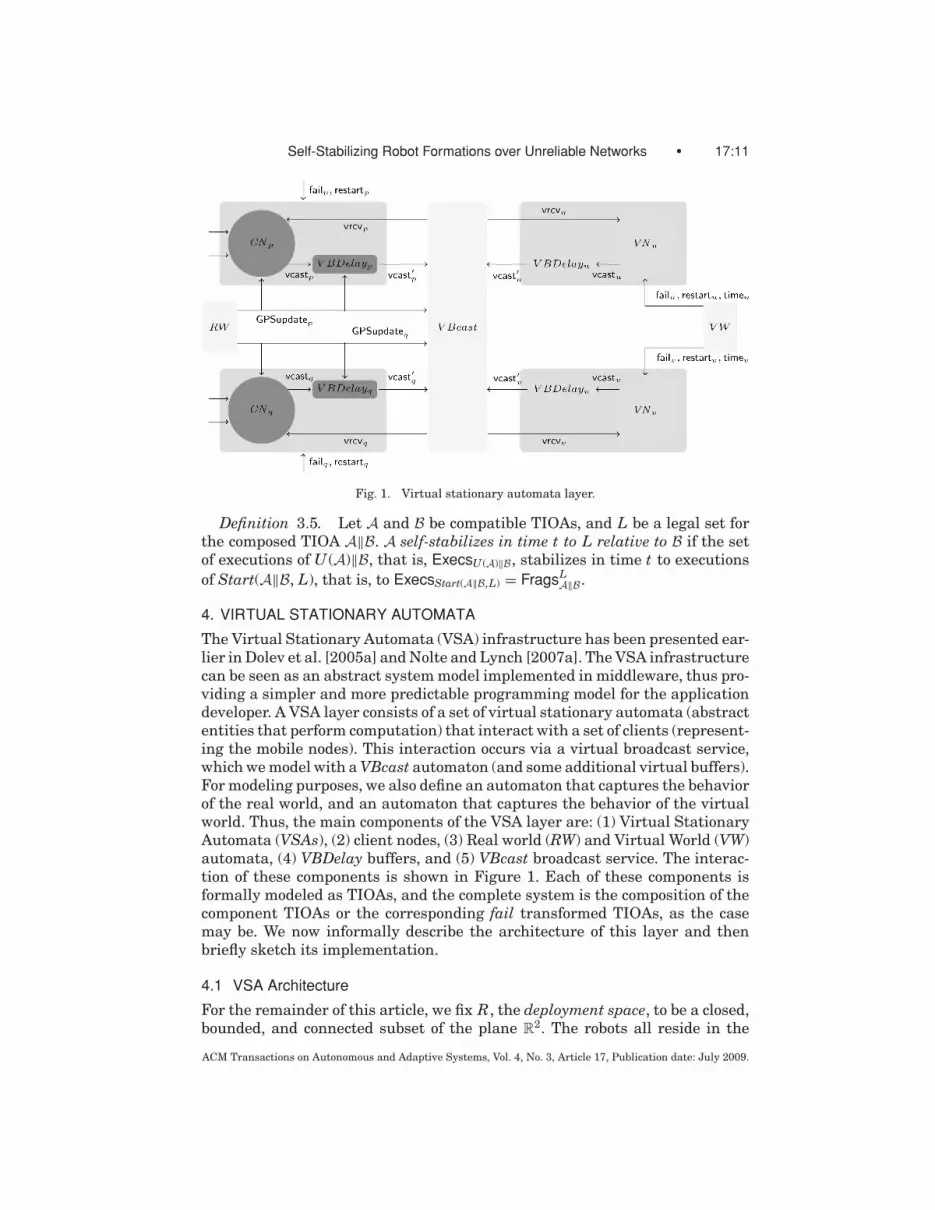
Fig. 1. Virtual stationary automata layer.

Definition 3.5. Let A and B be compatible TIOAs, and L be a legal set forthe composed TIOA A‖B. A self-stabilizes in time t to L relative to B if the setof executions of U (A)‖B, that is, ExecsU (A)‖B, stabilizes in time t to executionsof Start(A‖B, L), that is, to ExecsStart(A‖B,L) = FragsL

A‖B.

4. VIRTUAL STATIONARY AUTOMATA

The Virtual Stationary Automata (VSA) infrastructure has been presented ear-lier in Dolev et al. [2005a] and Nolte and Lynch [2007a]. The VSA infrastructurecan be seen as an abstract system model implemented in middleware, thus pro-viding a simpler and more predictable programming model for the applicationdeveloper. A VSA layer consists of a set of virtual stationary automata (abstractentities that perform computation) that interact with a set of clients (represent-ing the mobile nodes). This interaction occurs via a virtual broadcast service,which we model with a VBcast automaton (and some additional virtual buffers).For modeling purposes, we also define an automaton that captures the behaviorof the real world, and an automaton that captures the behavior of the virtualworld. Thus, the main components of the VSA layer are: (1) Virtual StationaryAutomata (VSAs), (2) client nodes, (3) Real world (RW) and Virtual World (VW)automata, (4) VBDelay buffers, and (5) VBcast broadcast service. The interac-tion of these components is shown in Figure 1. Each of these components isformally modeled as TIOAs, and the complete system is the composition of thecomponent TIOAs or the corresponding fail transformed TIOAs, as the casemay be. We now informally describe the architecture of this layer and thenbriefly sketch its implementation.

4.1 VSA Architecture

For the remainder of this article, we fix R, the deployment space, to be a closed,bounded, and connected subset of the plane R

2. The robots all reside in the



space defined by R. We fix U to be a totally ordered index set, which we used toidentify regions of the plane (as defined in the context of a network tiling). Wefix P to be another index set, which we use to identify the participating robots.

Network tiling. A network tiling divides the deployment space R into a setof regions {Ru}u∈U , such that: (i) For each u ∈ U , Ru is a closed, connected subsetof R, and (ii) for any u, v ∈ U , Ru and Rv may overlap only at their boundaries.For example, R might be a large rectangle in the plane, and the network tilingmight divide R into squares of edge-length b. We refer to this tiling as the gridtiling of R.

For any u, v ∈ U , the regions Ru and Rv are said to be neighbors if Ru∩Rv �= ∅,that is, if they shared a boundary. This neighborhood relation nbrs inducesa graph on the set of regions where there is an edge between every pair ofneighbors. We assume that the network tiling divides R in such a way that theresulting graph is connected. For any u ∈ U , we denote the set of neighboringregion identifiers by nbrs(u), and nbrs+(u) �= nbrs(u)∪{u}. We define the distancebetween two regions u and v, denoted by regDist(u, v), as the number of hopson the shortest path between u and v in the graph. The diameter of the graph,that is, the distance between the farthest regions in the tiling, is denoted byD, and the largest Euclidean distance between any two points in any region isdenoted by r.

We return to our example of a grid tiling where R is divided into b×b squareregions, for some constant b > 0. Nonborder regions in this tiling have eightneighbors. For a grid tiling with a given b, the diagonal of the tile is of length√

2 b, and hence for any two neighboring tiles u and v, the maximum distancebetween a point in u and a point in v is 2

√2 b. This implies that r could be any

value greater than or equal to 2√

2 b.

Real World (RW) automaton. We model the behavior of the real world viathe RW automaton. There are two key aspects of the real world: Time passes inthe real world, and the robots move in the real world. Thus, the RW automatonprovides the participating robots with occasional, reliable time and locationinformation, notifying each robot of the current real time and of its currentlocation. (A robot does not learn about the location of other robots, of course.)Such updates happen every so often; in particular, the time between two updatesis at most εsample.

Formally, the RW automaton is parameterized by: (a) vmax > 0, a maximumspeed, and (b) εsample > 0, a maximum time gap between successive updates foreach robot. The RW automaton maintains three key variables: (a) a continuousvariable now representing true system time; now increases monotonically atthe same rate as real-time starting from 0; (b) an array vel [P → R ∪ {⊥}];for p ∈ P , vel(p) represents the current velocity of robot p (initially vel(p) isset to ⊥, and it is updated by the robots when their velocity changes); (c) anarray loc[P → R]; for p ∈ P , loc(p) represents the current location of robotp. Over any interval of time, robot p may move arbitrarily in R provided itspath is continuous and its maximum speed is bounded by vmax. Automaton RWperforms GPSupdate(l , t)p actions, l ∈ R, t ∈ R≥0, p ∈ P , to inform robot p



about its current location and time. For each p, some GPSupdate(, )p actionmust occur every εsample time.

Virtual World (VW) automaton. While the mobile robots live in the realworld, the VSAs do not; they reside in a virtual world, and we model the behaviorof the virtual world separately from that of the real world. In some ways this isredundant, as we could define a single entity to model both the real and virtualworlds. It is convenient, however, to model these separately, emphasizing theaspects that are connected to the real world (and the mobile robots), and theaspects that are connected to the virtual world (and the VSAs).

The virtual world automaton VW provides occasional, reliable time infor-mation for VSAs. Similar to RW’s GPSupdate action for clients, VW performstime(t)u output actions notifying VSA u of the current time. Unlike the RW,however, it does not provide any location information; the virtual world is astatic one, and the VSAs do not move. The time updates occur every so often;one such update occurs at time 0, and they are repeated at least every εsampletime thereafter. The VW nondeterministically issues failu and restartu outputsfor each u ∈ U , modeling the fact that VSAs may fail and restart. (Again, noticethis is different from the mobile robots and the real world.)

Mobile client nodes. We now discuss how the mobile robots themselves aremodeled. For each p ∈ P , the mobile client node CNp is a TIOA modeling theclient-side program executed by the robot with identifier p. CNp has a localclock variable clock that progresses at the rate of real time, and is initially ⊥.CNp may have arbitrary local variables (albeit none with the name failed).

Its external interface includes a GPSupdate input, to receive updates fromthe real world. It also includes a facility for sending and receiving messagesto/from VSAs. As mentioned previously, we refer to this as the virtual broadcastservice, and thus each client has an output vcast(m)p for sending a message toa VSA, and an input vrcv(m)p for receiving a message from a VSA. (This isdiscussed in more detail shortly.) A client CNp may have additional arbitraryother actions (as long as none is name fail or restart). The pseudocode in Figure 2,while a part of our algorithm at the same time provides an example of how tospecify a program for a client node.

As discussed in the previous section, we model the clients, ignoring theirbehavior when crash failures occur. When defining the behavior of the entireVSA layer, we use failure transforms to model crash failures.

Virtual Stationary Automata (VSAs). We now discuss how VSAs are mod-eled. A VSA is a clock-equipped abstract virtual machine. For each u ∈ U ,there is a corresponding VSA VNu which is associated with the geographic re-gion Ru. VNu has a local clock variable clock which progresses at the rate ofreal time (it is initially ⊥). VNu has the following external interface, whichprovides it time updates from the VW automaton, and provides it the capac-ity to send and receive messages via the virtual broadcast service: (a) Inputtime(t)u, t ∈ R

≥0: models a time update at time t; it sets node VNu’s clock tot. (b) Output vcast(m)u, m ∈ Msg : models VNu broadcasting message m; (c)Input vrcv(m)u, m ∈ Msg : models VNu receiving a message m. VNu may have



Fig. 2. Client node CN(δ)p automaton.

additional arbitrary variables (as long as none is named failed) and arbitraryinternal actions (as long as none is name fail or restart). All such actions mustbe deterministic.

VBDelay automata. When clients and VSA nodes send messages, the delayin message delivery may be unpredictable. In particular, the messages may bedelayed for longer than might be expected due to the costs inherent to emulatingthe virtual world. We model these delays with a VBDelay buffer that holds backvirtual messages for some additional nondeterministic period of time.

For each client and each VSA node, there is a VBDelay buffer that delaysmessages for up to e time by intercepting sent messages. Formally, this impliesthat the buffer takes as input a vcast(m) from a node. After some interval oftime at most e, the message is handed to the virtual broadcast service. In thecase of VSA nodes, the delay e = 0.

VBcast automaton. Each client and VSA has access to the virtual broadcastcommunication service VBcast. This service is the primary means by which theclients communicate with the VSAs. The service is parameterized by a constantd > 0 which models the upper bound on message delays. VBcast takes eachvcast′(m, f )i input from client and virtual node delay buffers and delivers themessage m via vrcv(m) at each client or virtual node. It delivers the message toevery client and VSA that is in the same region as the initial sender, when themessage was first sent, along with those in neighboring regions. The VBcastservice guarantees that in each execution α of VBcast there is a correspondencebetween vrcv(m) actions and vcast′(m, f )i actions, such that: (i) Each vrcv occurs



after and within d time of the corresponding vcast′; (ii) at most one vrcv at aparticular process is mapped to each vcast′; (iii) a message originating fromsome region u must be received by all robots that are in Ru or its neighborsthroughout the transmission period.

Layers and algorithms. Since our goal is to model failure-prone robots, wedefine a VLayer to be the composition of the various components describedpreviously, where each of the clients has been fail-transformed. In other words,each client may fail by crashing. A VSA layer algorithm or a V -algorithm isan assignment of a TIOA program to each client and VSA (i.e., it specifiedwhich program execution on each client and VSA). We denote the set of allV-algorithms as VAlgs. Formally, we have the following.

Definition 4.1. Let alg be an element of Valgs. VLNodes[alg], the fail-transformed nodes of the VSA layer parameterized by alg, is the composi-tion of Fail(alg(i)) with a VBDelay buffer, for all i ∈ P ∪ U . VLayer[alg],the VSA layer parameterized by alg, is the composition of VLNodes[alg] withRW‖V W‖V Bcast.

4.2 VSA Layer Emulation

In Dolev et al. [2005a] and Nolte and Lynch [2007a], we show how mobile nodescan emulate the VSA layer in a wireless network. Additional details appearin Nolte [2008]. We begin with a realistic wireless network in which mobilerobots can communicate via wireless broadcast; we then show how to emulateVSAs in such a way as to implement the VSA layer described before. Here weattempt to give some of the basic ideas underlying the implementation.

First, the question arises as to under which conditions a VSA layer can be im-plemented. In Nolte [2008], the basic system model is quite similar to the modeldescribed in this article, except that the virtual broadcast service is replacedwith a more realistic broadcast service that allows for communication betweenthe mobile nodes. More specifically, the model consists of: (i) mobile nodes, mod-eled exactly as in this article; (ii) a RW automaton that models the real world,exactly as in this article; and (iii) a broadcast service that allows for communi-cation between mobile nodes. The broadcast service guarantees that messagesare delivered within some radius rreal, and we assume that rreal ≥ r+εsamplevmax.This ensures that if a mobile node broadcasts a message, then every other mo-bile node that is “within range” during the message delivery interval will receivethat message. In this case, a mobile node is within range if it is in the sameregion as the mobile node performing the broadcast, or in a neighboring region.(The second term compensates for the uncertainty in time and location.) Thebroadcast service guarantees that every message is delivered within time dreal .Lastly, the broadcast service satisfies the usual properties, namely, integrity (amessage is delivered only if it was previously sent) and nonduplicative delivery.Given such a broadcast service, Nolte [2008] shows how to emulate a VSA layersatisfying the described properties.

We continue by giving a brief overview of how mobile robots can cooperateto emulate VSAs, thus implementing a VSA layer. The emulation algorithm is



based on a replicated-state-machine paradigm. Specifically, mobile robots in aregion Ru cooperate to implement the region u’s virtual node.

The emulation relies on a totally ordered broadcast service (TOBcast)that guarantees that each mobile robot in a region receives messages in thesame order. (This ordered broadcast service is itself implemented via times-tamps and adding appropriate timing delays to ensure a uniform deliverysequence.)

All the participants in the emulation protocol for a given VSA act as replicas.Of these replicas, every so often, one is chosen to be the leader. (The leader elec-tion service is implemented by a competition among possible candidates.) Theleader is responsible for two tasks. First, it broadcasts the messages that theemulated VSA transmits via vcasts. In this way, the leader helps to emulatethe virtual broadcast service. Second, every so often, it broadcasts an up-to-date version of the VSA state. This broadcast is used both to keep the backupssynchronized (and hence stabilizing the emulation algorithm), and also to allownew emulators to start participating.

In order to maintain the necessary timing guarantees, the virtual machinestate is frozen while these synchronization messages are sent Then, the virtualmachine runs at an accelerated pace, simulating the VSN at faster-than-realtime until the emulation is caught up.

For further details on the emulation of VSA layers, we refer the interestedreader to Dolev et al. [2005a], Nolte and Lynch [2007a], and Nolte [2008].

5. MOTION COORDINATION USING VIRTUAL NODES

We begin by formally stating the motion coordination problem. We then presentan algorithm for the VSA Layer (specifically, a V-algorithm) for solving themotion coordination problem.

5.1 Problem Statement

The goal of motion coordination is to coordinate a set of mobile robots suchthat they deploy themselves evenly along some curve in the deployment spaceR. The first step, then, is to define the curve in the plane. Formally, we fix : A → R to be a simple, differentiable curve on R that is parameterized byarc length, where the domain set A of parameter values is an interval in thereal line. For example, assuming that the curve is of length at least x, then (x)is the point at distance x along .

We also fix a particular network tiling such that each point in is in someregion. Specifically, for the collection of regions {Ru}u∈U , for each point p in ,there is some region Ru such that the point p is in Ru.

For each region, we consider the portion of the curve that intersects thatregion. Let Au

�= {p ∈ A : region((p)) = u} be the domain of in region u. Weassume that Au is convex for every region u; it may be empty for some u. Thelocal part of the curve in region u is the restriction u : Au → Ru. We write|Au| for the length of the curve u.

In order to more easily discuss the length of the curve, we consider a quan-tized version of the curve; that is, for some constant σ , we round the length of



the curve to the nearest multiple of σ . For example, if the curve is of length 10,and if σ = 3, then the quantized length of the curve is 12.

More formally, given some quantization constant σ > 0, we define the quan-tization of a real number x as qσ (x) = � x

σ�σ . We fix σ , and write qu as an

abbreviation for qσ (|Au|). Notice that, intuitively, qu is the approximate lengthof that intersects region Ru, rounded up to the nearest multiple of σ .

We define qmin to be the minimum nonzero qu, that is, the minimum lengthof the curve in any region. We define qmax as the maximum qu, that is, themaximum length of the curve in any region.

Our goal is to design an algorithm for mobile robots such that, once thefailures and recoveries cease, within finite time all the robots are located on

and as time progresses they eventually become equally spaced on . Formally,if no fail and restart actions occur after time t0, then the following holds true.

(1) There exists a constant T , such that for each u ∈ U , within time t0 + Tthe set of robots located in Ru becomes fixed and its cardinality is roughlyproportional to qu; moreover, if qu �= 0 then the robots in Ru are located on4

u.(2) In the limit, as time goes to infinity, all robots in Ru are uniformly spaced5

on u.

5.2 Overview of Solution: Motion Coordination Algorithm (MC)

The VSA layer is used as a means to coordinate the movement of the mo-bile robots. A VSA controls the motion of the clients in its region by settingand broadcasting target waypoints for the clients. Each VSA VNu periodically:(i) receives information from clients in its region Ru, (ii) exchanges informationwith its neighboring VSAs, and (iii) sends out a message containing a calculatedtarget point for each client node “assigned” to region u.

The VSA VNu performs two tasks when setting the target points: (i) It reas-signs some of the clients that are assigned to itself to neighboring VSAs, and(ii) it sends a target position on to each client that is assigned to itself. The ob-jective of the first task is to spread the mobile robots proportionally among thevarious regions. By assigning some clients to neighboring regions, a VSA pre-vents its neighbors from getting depleted of robots. The objective of the secondtask is to space the nodes uniformly on within each region.

The client algorithm, by contrast, is quite simple. Each client receives atarget waypoint from the VSA in its region. It then computes a velocity vectorfor reaching this target point, and proceeds in this direction as fast as possible.

Of note, each VSA uses only local information about . In particular, itsdecisions are based only on the (quantized) length of the curve in its region,and in the neighboring regions. For the sake of simplicity, however, we assumethat all mobile robots and all VSAs know the complete curve , even though

4For a given point x ∈ R, if there exists p ∈ A such that (p) = x, then we say that the point x ison the curve ; abusing the notation, we write this as x ∈ .5A sequence x1, . . . , xn of points in R is said to be uniformly spaced on a curve if there exists asequence of parameter values p1 < p2 . . . < pn, such that for each i, 1 ≤ i ≤ n, (pi) = xi , and foreach i, 1 < i < n, pi − pi−1 = pi+1 − pi .



only local information is actually used. (In fact, the mobile robot does not needany information about the curve , as it receives all of its motion planning fromVSAs.)

5.3 Client Node Algorithm (CN)

We first describe the algorithm that runs on the mobile robots. The algorithm forthe client node CNp, for a fixed p ∈ P , is presented in Figure 2. The algorithmfollows a round structure, where rounds begin at times that are multiples of δ.We refer to the algorithm itself as CN(δ)p.

At the beginning of each round, each mobile robot sends a cn-update messageto the VSA in whose region it is currently residing (see lines 30–34) and stopsmoving (lines 36–41, when x∗ = ⊥). The cn-update message tells the local VSAthe robot’s id and its current location in R.

The local VSA then sends a response to the client, that is, a target-updatemessage (see lines 43–48). Each such message describes the new target locationx∗

p for CNp, and possibly includes an assignment to a different region. Therobot first computes the direction vector toward this new point based on itscurrent position xp; that is, it computes the (unit-length) direction vector vp =(xp − x∗

p)/||xp − x∗p||. It then proceeds to move in this direction with maximum

velocity, namely, it sets its velocity to vmaxvp (see lines 36–41). This is thenoutput as a velocity signal to the RW.

Formally, the stops when condition enforces the facts: (i) that the robot stopsat the beginning of every round, (ii) that it updates its velocity as soon as itreceives a target waypoint, and (iii) that it necessarily stops if it does not haveenough information to calculate its waypoint. The first situation is resolved bybroadcasting a message via a vcast, while the latter two situations are resolvedby outputting a new velocity.

5.4 Virtual Stationary Node Algorithm (VN)

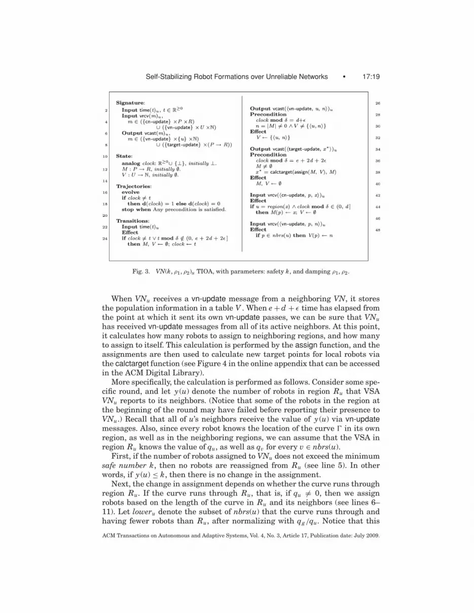
We now describe the program for the VSAs. The pseudocode is presented inFigure 3, and the TIOA is parameterized by three parameters: k ∈ Z

+, andρ1, ρ2 ∈ (0, 1). The integer k describes the minimum number of robots thatshould be assigned to a region. We thus refer to k as the safe number of robots.When k is larger, it is less likely that a VSA will fail as all k robots must failbefore the VSA fails. When k is smaller, the robots are spread more evenly alongthe curve (i.e., fewer are “wasted” on regions not on the curve). The parametersρ1 and ρ2 effect the rate of convergence. We refer to the algorithm executing inregion Ru as VN(k, ρ1, ρ2)u, u ∈ U .

At the beginning of each round, VNu collects cn-update messages sent fromrobots located in region Ru (see lines 42–45). It then aggregates the locationand round information in a table M . When d + ε time has passed from thebeginning of the round, we can be certain that all the cn-update have beendelivered. At this point, VNu computes the number of client nodes that arecurrently assigned to region Ru, and sends this information in a vn-updatemessage to all of its neighbors (lines 27–32).



Fig. 3. VN(k, ρ1, ρ2)u TIOA, with parameters: safety k, and damping ρ1, ρ2.

When VNu receives a vn-update message from a neighboring VN, it storesthe population information in a table V . When e + d + ε time has elapsed fromthe point at which it sent its own vn-update passes, we can be sure that VNuhas received vn-update messages from all of its active neighbors. At this point,it calculates how many robots to assign to neighboring regions, and how manyto assign to itself. This calculation is performed by the assign function, and theassignments are then used to calculate new target points for local robots viathe calctarget function (see Figure 4 in the online appendix that can be accessedin the ACM Digital Library).

More specifically, the calculation is performed as follows. Consider some spe-cific round, and let y(u) denote the number of robots in region Ru that VSAVNu reports to its neighbors. (Notice that some of the robots in the region atthe beginning of the round may have failed before reporting their presence toVNu.) Recall that all of u’s neighbors receive the value of y(u) via vn-updatemessages. Also, since every robot knows the location of the curve in its ownregion, as well as in the neighboring regions, we can assume that the VSA inregion Ru knows the value of qu, as well as qv for every v ∈ nbrs(u).

First, if the number of robots assigned to VNu does not exceed the minimumsafe number k, then no robots are reassigned from Ru (see line 5). In otherwords, if y(u) ≤ k, then there is no change in the assignment.

Next, the change in assignment depends on whether the curve runs throughregion Ru. If the curve runs through Ru, that is, if qu �= 0, then we assignrobots based on the length of the curve in Ru and its neighbors (see lines 6–11). Let loweru denote the subset of nbrs(u) that the curve runs through andhaving fewer robots than Ru, after normalizing with qg/qu. Notice that this



normalization factor ensures that the number of robots in each region will beproportional to the length of the curve running through each region. For eachg ∈ loweru, the VSA VNu reassigns a number of robots to Rg based on thefollowing. First, we calculate a value ra′ that represents the ideal number ofrobots to transfer. We have

ra′ �= ρ2 · qg

qu· y(u) − y(g )

2(|loweru| + 1)(1)

where ρ2 < 1 is a damping factor. Then, the VSA VNu transfers either ra′

robots, or the remaining number of robots over k assigned to VNu. In otherwords, it transfers: ra �= min(ra′, n − k) robots to region Rg . This ensures thatat least k robots are left in region Ru. Next, if the curve does not run the regionRu, that is , qu = 0, then the transfer of robots depends on whether Ru has anyneighbors on the curve. If Ru has no neighbors on the curve, that is, qg = 0for all g ∈ nbrs(u), then the robots are distributed among neighbors that havefewer robots (lines 12–17). Let loweru denote the subset of nbrs(u) with fewerrobots than Ru. In this case, for each g ∈ loweru, we define ra′ as follows.

ra′ �= ρ2 · y(u) − y(g )2(|loweru| + 1)

(2)

The VSA VNu reassigns ra = min(ra′, n − k) robots to Rk .The last case is when VNu is on the boundary of the curve, meaning that the

curve does not run through Ru, but it does run through one of the neighbors ofRu, that is, there is a g ∈ nbrs(u) with qg �= 0 (see lines 18–20 ). In this case,y(u) − k of VNu’s CNs are assigned equally to neighbors that are on the curve.Specifically, we calculate ra as follows.

ra �=⌊

y(u) − k|{v ∈ nbrs(u) : qv �= 0}

⌋(3)

Again, notice that in each of these cases, at least k robots are left assigned toregion Ru.

The calctarget function assigns a target waypoint to every nonfailed robot inregion Ru. This target point locMu(p) is in region Rg , where g = u or one ofu’s neighbors. The target point locMu(p) is computed as follows: If a robot p isassigned to region Rg , g �= u, then its target is set to the center of region Rg(line 28); if the robot is assigned to Ru but is not located on the curve u thenits target is set to the nearest point on the curve, nondeterministically choosingone if there are several (line 29); if the robot is either the first or last robot onu then its target is set to the corresponding endpoint of u (lines 31–32); if therobot is on the curve but is not the first or last client node then its target ismoved to the midpoint of the locations of the preceding and succeeding robotson the curve (line 35). For the last two computations a sequence seq of nodeson the curve sorted by curve location is used (line 26).

5.5 Complete System

The complete algorithm, MC, is the instantiation of each component inFigure 1 with fail-transformed CN and VN algorithms. Formally, it is the



parallel composition of the following TIOAs: (a) RW, (b)VW, (c) VBcast, (d)Fail(VBDelayp‖CNp), one for each p ∈ P , and (e) Fail(VBDelayu‖V Nu). Re-call that Fail(A) denotes the fail-transformed version of TIOA A.

Round length. Given the maximum distance r between points in neighbor-ing regions, it can take up to r/vmax time for a client to reach its target. Afterthe client arrives in the region it was assigned to, it could find the local VN hasfailed. Let dr be the time it takes a VN to start up after a new node enters theregion. To ensure a round is long enough for a client node to send the cn-update,allow VNs to exchange information, allow clients both to receive a target-updatemessage and arrive at new assigned target locations, we require that the CNparameter δ to be greater than 2e + 3d + 2ε + r/vmax + dr .

6. CORRECTNESS OF ALGORITHM

In this section, we show that starting from an initial state the system describedin Section 5.2 satisfies the requirements specified in Section 5.1. In the followingsection we show self-stabilization. The proofs of the results in this section par-allel those presented in Lynch et al. [2005], albeit the semantics of the virtuallayers used here is different.

We define round t as the interval of time [δ(t −1), δ · t); that is, round t beginsat time δ(t − 1) and is completed by time δ · t. We say CNp, p ∈ P , is active inround t if node p is not failed throughout round t. A VNu, u ∈ U , is active inround t if there is some active CNp such that region(xp) = u for the durationof rounds t − 1 and t. Thus, by definition, none of the VNs is active in the firstround. We also define the following notation:

—In(t) ⊆ U is the subset of VN ids that are active in round t and qu �= 0;—Out(t) ⊆ U is the subset of VNs that are active in round t and qu = 0;—C(t) ⊆ P is the subset of active CNs at round t;—Cin(t) ⊆ P is the set of active CNs located in regions with id in In(t) at the

beginning of round t;—Cout(t) ⊆ P is subset of active CNs located in regions with id in Out(t) at the

beginning of round t.

For every pair of regions u, w and for every round t, we define y(w, t)u to bethe value of V (w)u (i.e., the number of clients u believes are available in regionw) immediately prior to VNu performing a vcastu in round t, namely, at timee + 2d + 2ε after the beginning of round t. If there are no new client failuresor recoveries in round t, then for every pair of regions u, w ∈ nbrs+(v), we canconclude that y(v, t)u = y(v, t)w, which we denote simply as y(v, t).

We define ρ3�= q2

max/(1 − ρ2)σ . The rate ρ3 effects the rate of convergence,and will be used in the analysis. Notice that ρ3 > 1.

6.1 Approximately Proportional Distribution

For the rest of this section we fix a particular round number t0 and assumethat, for all p ∈ P , no failp or recoverp events occur at or after round t0. The first



lemma states some basic facts about the assign function. All the proofs appearin the Appendix accessible in the ACM Digital Library.

LEMMA 6.1. In every round t ≥ t0: (1) If y(u, t) ≥ k for some u ∈ U, theny(u, t + 1) ≥ k; (2) In(t) ⊆ In(t + 1); (3) Out(t) ⊆ Out(t + 1).

We now identify a round t1 ≥ t0 after which the set of regions In(t) and Out(t)remain fixed.

LEMMA 6.2. There exists a round t1 ≥ t0 such that for every round t ∈ [t1, t1+(1 + ρ3)m2n2]: (1) In(t) = In(t1); (2) Out(t) = Out(t1); (3) Cin(t) ⊆ Cin(t + 1); and(4) Cout(t+1) ⊆ Cout(t). Round t1 occurs no later than time t0 +2m2 ·(1+ρ3)m2n2.

Fix t1 for the rest of this section such that it satisfies Lemma 6.2. The nextlemma states that eventually, regions bordering on the curve stop assigningclients to regions that are on the curve. In other words, assume that u is a regionwhere qu = 0, but that u has a neighbor v where qv �= 0; then, eventually, fromsome round onwards, u never again assigns clients to v.

LEMMA 6.3. There exists some round t2 ∈ [t1, t1 + (1 +ρ3)m2n2] such that forevery round t ∈ [t2, t2 + (1 + ρ3)m2n]: If u ∈ Out(t) and v ∈ In(t) and if u and vare neighboring regions, then u does not assign any clients to v in round t.

Fix t2 for the rest of this section such that it satisfies Lemma 6.3. Lemma 6.2implies that in every round t ≥ t1, In(t) = In(t1) and Out(t) = Out(t1); we denotethese simply as In and Out. The next lemma states a key property of the assignfunction after round t1. For a round t ≥ t1, consider some VNu, u ∈ Out(t), andassume that VNw is the neighbor of VNu assigned the most clients in roundt. Then we can conclude that VNu is assigned no more clients in round t + 1than VNw is assigned in round t. A similar claim holds for regions in In(t), butin this case with respect to the density of clients with respect to the quantizedlength of the curve. The proof of this lemma is based on careful analysis of thebehavior of the assign function.

LEMMA 6.4. In every round t ∈ [t2, t2 + (1 + ρ3)m2n], for u, v ∈ U and u ∈nbrs(v):

(1) If u, v ∈ Out(t) and y(v, t) = maxw∈nbrs(u)∩Out(t) y(w, t) and y(u, t) < y(v, t),then y(u, t + 1) < y(v, t).

(2) If u, v ∈ In(t) and y(v, t)/qv = maxw∈nbrs(u)∩In(t)[ y(w, t)/qw] and y(u, t)/qu <

y(v, t)/qv, theny(u, t + 1)

qu≤ y(v, t)

qv− (1 − ρ2)

σ

q2max

.

The next lemma states that there exists a round Tout such that in every roundt ≥ Tout , the set of CNs assigned to region u ∈ Out(t) does not change.

LEMMA 6.5. There exists a round Tout ∈ [t2, t2 + m2n such that in any roundt ≥ Tout , the set of CNs assigned to VNu, u ∈ Out(t), is unchanged.



Next, we fix Tout to be the first round after t0, at which the property stated byLemma 6.5 holds. Lemma 6.5, together with Lemmas 6.1, 6.2, and 6.3, implythat in every round t ≥ Tout , CIn(t) = CIn(t1) and COut(t) = COut(t1); we denotethese simply as CIn and COut. The next lemma states a property similar to thatof Lemma 6.5 for VNu, u ∈ In, and the argument is similar to the proof ofLemma 6.5, and uses part (2) of Lemma 6.4. We also bound the total numberof clients located in regions with ids in Out to be O(m3).

LEMMA 6.6. There exists a round Tstab ∈ [Tout , Tout + ρ3m2n] such that inevery round t ≥ Tstab, the set of CNs assigned to VNu, u ∈ In, is unchanged.Further, in every round t ≥ Tout , |Cout(t)| = O(m3).

For the rest of the section we fix Tstab to be the first round after Tout , atwhich the property stated by Lemma 6.6 holds. Lemma 6.7 states that thenumber of clients assigned to each VNu, u ∈ In, in the stable assignment afterTstab is proportional to qu within a constant additive term. The proof follows byinduction on the number of hops from between any pair of VNs.

LEMMA 6.7. In every round t ≥ Tstab, for u, v ∈ In(t):∣∣∣∣ y(u, t)qu

− y(v, t)qv

∣∣∣∣ ≤[

10(2m − 1)qminρ2

].

6.2 Uniform Spacing

From line 29 of Figure 4, it follows that by the beginning of round Tstab + 2, allCNs in Cin are located on the curve . Thus, the algorithm satisfies our firstgoal. The next lemma states that the locations of the CNs in each region u,u ∈ In, are uniformly spaced on u in the limit, and it is proved by analyzingthe behavior of calctarget as a discrete time dynamical system.

LEMMA 6.8. Consider a sequence of rounds t1 = Tstab, . . . , tn. As n → ∞, thelocations of CNs in u, u ∈ In, are uniformly spaced on u.

Thus we conclude by summarizing the results in this section.

THEOREM 6.9. If there are no fail or restart actions for robots at or after someround t0, then within a finite number of rounds after t0:

(1) The set of CNs assigned to each VNu, u ∈ U, becomes fixed, and the size ofthe set is proportional to the quantized length qu, within a constant additiveterm 10(2m−1)

qminρ2.

(2) All client nodes in a region u ∈ U for which qu �= 0 are located on u anduniformly spaced on u in the limit.

7. SELF-STABILIZATION OF ALGORITHM

In this section we show that the VSA-based motion coordination scheme is self-stabilizing. Specifically, we show that when the VSA and client components inthe VSA layer start out in some arbitrary state owing to failures and restarts,they eventually return to a reachable state. Thus, the traces of VLayer[MC]



running with some reachable state of Vbcast‖RW‖V W eventually become in-distinguishable from a reachable trace of VLayer[MC]. Recall Definition 4.1 andnote that the virtual layer algorithm alg is instantiated here with the motioncoordination algorithm MC of Section 5.

We first show that our motion coordination algorithm VLNodes[MC] is self-stabilizing to some set of legal states LMC. Then, we show that these legalstates correspond to reachable states of VLayer[MC]; hence, the traces of ourmotion coordination algorithm, where clients and VSAs start in an arbitrarystate, eventually look like reachable traces of the correct motion coordinationalgorithm.

An emulation is a kind of implementation relationship between two setsof TIOAs. A VSA layer emulation algorithm is a mapping that takes a VSAlayer algorithm, alg, and produces TIOA programs for an underlying systemconsisting of emulator physical nodes (corresponding to clients), such that whenthose programs are run with external oracles such as RW, the resulting systemhas traces that are closely related to the traces of a VSA layer. In particular,the traces restricted to nonbroadcast actions at the client nodes are the same.

In Dolev et al. [2005a] and Nolte and Lynch [2007a] we have shown howto implement a self-stabilizing VSA layer. In particular, that implementationguarantees that: (1) Each algorithm alg ∈ VAlgs stabilizes in some tVstab time totraces of executions of U (VLNodes[al g ])‖R(RW‖V W‖Vbcast), and (2) for anyu ∈ U , if there exists a client that has been in region u and alive for dr time andno alive clients in the region failed or left the region in that time, then VSA Vuis not failed. Thus, if the coordination algorithm MC is such that VLNodes[MC]self-stabilizes in some time t to LMC relative to R(RW‖VW‖Vbcast), then we canconclude that physical node traces of the emulation algorithm on MC stabilizein time tVstab + t to client traces of executions of the VSA layer started in legalset LMC and that satisfy the above failure-related properties.

7.1 Legal Sets

First we describe two legal sets for VLayer[MC], L1MC and LMC. The first legal

set L1MC describes a set of states that result after the first GPSupdate occurs at

each client node and the first timer occurs at each virtual node.

Definition 7.1. A state x of VLayer[MC] is in L1MC iff the following hold:

(1) x�X V bcast‖RW‖V W ∈ ReachV bcast‖RW‖V W .(2) ∀u ∈ U : ¬failedu : clocku ∈ {RW.now, ⊥} ∧ (Mu �= ∅ ⇒ clocku mod δ ∈

(0, e + 2d + 2ε]).(3) ∀p ∈ P : ¬failedp ⇒ vp ∈ {RW.vel(p)/vmax, ⊥}.(4) ∀p ∈ P : ¬failedp ∧ xp �= ⊥:

(a) xp = RW.loc(p) ∧ clockp = RW.now.(b) x∗

p ∈ {xp, ⊥} ∨ ||x∗p − xp|| < vmax(δ�clockp/δ� − clockp − dr ).

(c) Vbcast.reg (p) = region(xp)∨clock mod δ ∈ (e+2d +2ε, δ −dr +εsample).

Part (1) requires that x restricted to the state of Vbcast‖RW‖VW to be areachable state of Vbcast‖RW‖VW. Part (2) states that nonfailed VSAs have



clocks that are either equal to real time or ⊥, and have nonempty M only afterthe beginning of a round and up to e + 2d + 2ε time into a round. Part (3)states that nonfailed clients have velocity vectors that are equal either to ⊥ orequal to the client’s velocity vector in RW, scaled down by vmax. Finally, part (4)states that nonfailed clients with non-⊥ positions have: (4a) positions equal totheir actual location and local clocks equal to the real time, (4b) targets thatare one of ⊥, the location, or a point reachable from the current location withindr before the end of the round, and (4c) Vbcast last region updates that matchthe current region or the time is within a certain time window in a round. It isroutine to check that L1

MC is indeed a legal set for VLayer[MC].Now we describe the main legal set LMC for our algorithm. First we describe

a set of reset states, states corresponding to states of VLayer[MC] at the startof a round. Then, LMC is defined as the set of states reachable from these resetstates.

Definition 7.2. A state x of VLayer[MC] is in ResetMC iff:

(1) x ∈ L1MC;

(2) ∀p ∈ P : ¬failedp ⇒ [to send−p = to send+

p = λ ∧ (xp = ⊥ ∨ (x∗p �= ⊥ ∧ vp =

0))];(3) ∀u ∈ U : ¬failedu ⇒ to sendu = λ;(4) ∀〈m, u, t, P ′〉 ∈ vbcastq : P ′ = ∅;(5) RW.now mod δ = 0 ∧ ∀p ∈ P : ∀〈l , t〉 ∈ RW.updates(p) : t < RW.now. LMC

is the set of reachable states of Start(VLayer[MC], ResetMC).

ResetMC consists of states in which: (1) in L1MC, (2) nonfailed clients have

empty queues in its VBDelay and either has a position variable equal to ⊥or has both a non-⊥ target and 0 velocity, (3) nonfailed VSAs have an emptyqueue in their VBDelay, (4) there are no still-processing messages in Vbcast, and(5) the time is the starting time for a round and that no GPSupdates have yetoccurred at this time. Once again, it is routine to check that that LMC is a legalset for VLayer[MC].

7.2 Stabilization to LMC

First, we state the following result related to stabilization.

LEMMA 7.3. VLNodes[MC] is self-stabilizing to L1MC in time t > εsample rel-

ative to the automaton R(Vbcast‖RW‖VW).

To see this, consider the moment after each client has received a GPSupdateand each virtual node has received a time update, which takes at most εsampletime.

Next we show that starting from a state in L1MC, we eventually arrive at a

state in ResetMC, and hence a state in LMC.

LEMMA 7.4. Executions of VLayer[MC] started in states in L1MC stabilize in

time δ + d + e to executions started in states in LMC.



Combining our stabilization results we conclude that VLNodes[MC] startedin an arbitrary state and run with R(Vbcast‖RW‖VW) stabilizes to LMC in timeδ + d + e + εsample. From transitivity of stabilization and 7.4, the next resultfollows.

THEOREM 7.5. VLNodes[MC] is self-stabilizing to LMC in time δ + d + e +εsample relative to R(Vbcast‖RW‖VW).

7.3 Relationship between LMC and Reachable States

In the previous section we showed that VLNodes[MC] is self-stabilizing to LMCrelative to R(Vbcast‖RW‖VW). In order to conclude anything about the tracesof VLayer[MC] after stabilization, however, we need to show that traces ofVLayer[MC] starting in a state in LMC are reachable traces of VLayer[MC].This is accomplished by first defining a simulation relation RMC on the statesof VLayer[MC], and then proving that for each state x ∈ LMC, there exists astate y ∈ ReachVLayer[MC] such that x and y are related by RMC. This impliesthat the trace of any execution fragment starting with x is the trace of an exe-cution fragment starting with y, which is a reachable trace of VLayer[MC]. Wedefine the candidate relation RMC and prove that it is indeed a simulation rela-tion. Here, we describe some of the conditions two related states x and y mustsatisfy. Owing to limited space, the complete formal definition of the simulationrelation appears in Appendix C. Part (1) of the relation requires that they sharethe same real time and locations for CNs. Part (2) requires that for each client,the velocity at RW is equal or the velocity in y is ⊥, and GPSupdate recordsin the two states are for the same times. Part (3) requires that VW’s state andVbcast.now are the same in x and y. Part (4) requires that the unprocessedmessage tuples and the last recorded regions in Vbcast for clients are the samein both states. The proof of the following lemma is also routine and it breaksdown into a large case analysis.

LEMMA 7.6. RMC is a simulation relation for VLayer[MC].

To show that each state in LMC is related to a reachable state of VLayer[MC],it is enough to show that each state in ResetMC is related to a reachable stateof VLayer[MC]. The proof proceeds by providing a construction of an executionof VLayer[MC] for each state in LMC.

LEMMA 7.7. For each state x ∈ ResetMC, there exists a state y ∈ReachVLayer[MC] such that xRMCy.

From Lemmas 7.7 and 7.6 it follows that the set of trace fragments ofVLayer[MC] corresponding to execution fragments starting from ResetMC iscontained in the set of traces of R(VLayer[MC]). Bringing our results togetherwe arrive at the main theorem.

THEOREM 7.8. The traces of VLNodes[MC], starting in an arbitrary state andexecuted with automaton R(Vbcast‖RW‖VW), stabilize in time δ+d +e+εsampleto reachable traces of R(VLayer[MC]).

Thus, despite starting from an arbitrary configuration of the VSA and clientcomponents in the VSA layer, if there are no failures or restart of client nodes



(robots) at or after some round t0, then within a finite number of rounds aftert0, the clients are located on the curve and are uniformly spaced in the limit.

8. CONCLUSION

We have described how we can use the virtual stationary automaton infras-tructure to design protocols that are resilient to failure of participating agents.In particular, we presented a protocol by which the participating robots can beuniformly spaced on an arbitrary curve. The VSA layer implementation and thecoordination protocol are both self-stabilizing. Thus, each robot can begin in anarbitrary state, in an arbitrary location in the network, and the distribution ofthe robots will still converge to the specified curve. The proposed coordinationprotocol uses only local information, and hence should adapt well to flocking ortracking problems where the target formation is dynamically changing.

LIST OF SYMBOLS AND FUNCTIONS

δ Duration of each round of CN algorithmεsample Maximum duration between two successive GPS updatesExecsA Set of executions of TIOA AFragsL

A Set of execution fragments of TIOA A starting from L Target curve; a (fixed) simple differentiable curve on Ru restricted to RuFail (A) The TIOA obtained by fail-transforming TIOA ACNp Client node automatonRW Real world automatonVBcast Automaton model for virtual layer local broadcast serviceVNu Virtual node automatonVW Virtual world automatonReachA Reachable states of TIOA A�A Set of start states of TIOA ATracesA Set of traces of TIOA Ad Maximum message delay incurred by VBcast servicee Maximum delay introduced by VBDelay bufferQA Set of states of TIOA AR Deployment space for the mobile robotsR(A) The TIOA obtained replacing starting states of A by ReachARu A region in R corresponding to VNu according to some

fixed tilingStart(A, S) The TIOA obtained replacing starting states of A by SU (A) The TIOA obtained replacing starting states of A by QA

REFERENCES

ANDO, H., OASA, Y., SUZUKI, I., AND YAMASHITA, M. 1999. Distributed memoryless point convergencealgorithm for mobile robots with limited visibility. IEEE Trans. Robotics Autom. 15, 5, 818–828.



BLONDEL, V., HENDRICKX, J., OLSHEVSKY, A., AND TSITSIKLIS, J. 2005. Convergence in multi-agentcoordination consensus and flocking. In Proceedings of the Joint 44th IEEE Conference on Decisionand Control and European Control Conference. 2996–3000.

BROWN, M. D. 2007. Air traffic control using virtual stationary automata. M.S. thesis, Mas-sachusetts Institute of Technology.

CHANDY, K. M., MITRA, S., AND PILOTTO, C. 2008. Convergence verification: From shared mem-ory to partially synchronous systems. In Proceedings of the Formal Modeling and Analysis ofTimed Systems (FORMATS’08). Lecture Notes in Computer Science, vol. 5215. Springer Verlag,217–231.

CHOCKLER, G., GILBERT, S., AND LYNCH, N. 2008. Virtual infrastructure for collision-prone wirelessnetworks. In Proceedings of the Annual ACM SIGOPS Symposium on Principles of DistributedComputing (PODC).

CLAVASKI, S., CHAVES, M., DAY, R., NAG, P., WILLIAMS, A., AND ZHANG, W. 2003. Vehicle networks:Achieving regular formation. In Proceedings of the American Control Conference.

CORTES, J., MARTINEZ, S., KARATAS, T., AND BULLO, F. 2004. Coverage control for mobile sensingnetworks. IEEE Trans. Robotics Autom. 20, 2, 243–255.

DEFAGO, X. AND KONAGAYA, A. 2002. Circle formation for oblivious anonymous mobile robots withno common sense of orientation. In Proceedings of the 2nd International Workshop on Principlesof Mobile Computing (POMC’02). ACM, 97–104.

DEFAGO, X. AND SOUISSI, S. 2008. Non-uniform circle formation algorithm for oblivious mobilerobots with convergence toward uniformity. Theor. Comput. Sci. 396, 1-3, 97–112.

DOLEV, S. 2000. Self-Stabilization. MIT Press, Cambridge.DOLEV, S., GILBERT, S., LAHIANI, L., LYNCH, N., AND NOLTE, T. 2005a. Virtual stationary automata

for mobile networks. In Proceedings of the International Conference on Principles of DistributedSystems (OPODIS).

DOLEV, S., GILBERT, S., LAHIANI, L., LYNCH, N. A., AND NOLTE, T. A. 2005b. Virtual stationary au-tomata for mobile networks. Tech. rep. MIT-LCS-TR-979.

DOLEV, S., GILBERT, S., LYNCH, N., SHVARTSMAN, A., AND WELCH, J. 2003. Geoquorums: Implementingatomic memory in ad hoc networks. In Distributed Algorithms, F. E. Fich, Ed. Lecture Notes inComputer Science, vol. 2848. 306–320.

DOLEV, S., GILBERT, S., LYNCH, N. A., SCHILLER, E., SHVARTSMAN, A. A., AND WELCH, J. L. 2004. Virtualmobile nodes for mobile ad hoc networks. In Proceedings of the 18th International Symposiumon Distributed Computing (DISC). 230–244.

DOLEV, S., GILBERT, S., LYNCH, N. A., SHVARTSMAN, A. A., AND WELCH, J. 2005. Geoquorums: Imple-menting atomic memory in mobile ad hoc networks. Distrib. Comput.

EFRIMA, A. AND PELEG, D. 2007. Distributed models and algorithms for mobile robot systems. InProceedings of SOFSEM (1). Lecture Notes in Computer Science, vol. 4362. Springer, 70–87.

FAX, J. AND MURRAY, R. 2004. Information flow and cooperative control of vehicle formations. IEEETrans. Autom. Control 49, 1465–1476.

FLOCCHINI, P., PRENCIPE, G., SANTORO, N., AND WIDMAYER, P. 2001. Pattern formation by autonomousrobots without chirality. In Proceedings of the Colloquium on Structural Information and Com-munication Complexity (SIROCCO). 147–162.

GAZI, V. AND PASSINO, K. M. 2003. Stability analysis of swarms. IEEE Trans. Autom. Control 48, 4,692–697.

GOLDENBERG, D. K., LIN, J., AND MORSE, A. S. 2004. Towards mobility as a network control primi-tive. In Proceedings of the 5th ACM International Symposium on Mobile Ad Hoc Networking andComputing (MobiHoc’04). ACM Press, 163–174.

HERMAN, T. 1996. Self-stabilization bibliography: Access guide. Theoretical Comput. Sci.JADBABAIE, A., LIN, J., AND MORSE, A. S. 2003. Coordination of groups of mobile autonomous agents

using nearest neighbor rules. IEEE Trans. Autom. Control 48, 6, 988–1001.KAYNAR, D. K., LYNCH, N., SEGALA, R., AND VAANDRAGER, F. 2005. The Theory of Timed I/O Automata.

Synthesis Lectures on Computer Science. Morgan Claypool. Also available as Tech. rep. MIT-LCS-TR-917.

LIN, J., MORSE, A., AND ANDERSON., B. 2003. Multi-agent rendezvous problem. In Proceedings ofthe 42nd IEEE Conference on Decision and Control.



LYNCH, N., MITRA, S., AND NOLTE, T. 2005. Motion coordination using virtual nodes. In Proceedingsof the 44th IEEE Conference on Decision and Control (CDC’05).

MARTINEZ, S., CORTES, J., AND BULLO, F. 2005. On robust rendezvous for mobile autonomous agents.In Proceedings of the IFAC World Congress.

NOLTE, T. AND LYNCH, N. A. 2007a. Self-stabilization and virtual node layer emulations. In Pro-ceedings of the International Symposium on Self-Stablizing Systems (SSS). 394–408.

NOLTE, T. AND LYNCH, N. A. 2007b. A virtual node-based tracking algorithm for mobile networks.In IEEE International Conference on Distributed Computing Systems (ICDCS).

NOLTE, T. A. 2008. Virtual stationary timed automata for mobile networks. Ph.D. thesis, Mas-sachusetts Institute of Technology, Cambridge.

OLFATI-SABER, R., FAX, J., AND MURRAY, R. 2007. Consensus and cooperation in networked multi-agent systems. Proc. IEEE 95, 1, 215–233.

PRENCIPE, G. 2000. Achievable patterns by an even number of autonomous mobile robots. Tech.rep. TR-00-11. 17.

PRENCIPE, G. 2001. Corda: Distributed coordination of a set of autonomous mobile robots. InProceedings of the European Research Seminar on Advances in Distributed Systems (ERSADS).185–190.

SUZUKI, I. AND YAMASHITA, M. 1999. Distributed autonomous mobile robots: Formation of geometricpatterns. SIAM J. Comput. 28, 4, 1347–1363.

Received July 2008; accepted June 2009


self-stabilizing robot formations over unreliable networks

Documents