intro-stabilizing byzantine clock synchronization in ... - arxiv
TRANSCRIPT

1
Intro-Stabilizing Byzantine Clock Synchronizationin Heterogeneous IoT Networks
Shaolin Yu Jihong Zhu Jiali Yang Wei LuTsinghua University Beijing China
ysl8088163com
AbstractmdashFor reaching dependable high-precision clock syn-chronization (CS) upon IoT networks the distributed CSparadigm adopted in ultra-high reliable systems and the master-slave CS paradigm adopted in high-performance but unreliablesystems are integrated Meanwhile traditional internal clocksynchronization is also integrated with external time referencesto achieve efficient stabilization Low network connectivity lowcomplexity high precision and high reliability are all consideredTo tolerate permanent failures the Byzantine CS is integratedwith the common CS protocols To tolerate transient failures theself-stabilizing Byzantine CS is also extended upon open-worldIoT networks With these the proposed intro-stabilizing Byzan-tine CS solution can establish and maintain synchronization witharbitrary initial states in the presence of permanent Byzantinefaults With the formal analysis and numerical simulations it isshown that the best of the CS solutions provided for the ultra-highreliable systems and the high-performance unreliable systems canbe well integrated upon IoT networks to derive dependable high-precision CS even across the traditional closed safety-boundary
Index Termsmdashclock synchronization Internet of things Byzan-tine fault intro-stabilization
I INTRODUCTION
Clock synchronization (CS) is fundamental in designing tra-ditional Distributed Real-Time Systems (DRTS) [1 2 3 4 5]and todayrsquos Real-Time Embedded Systems (RTES) [6] Cyber-Physical Systems (CPS) Wireless Sensor Networks (WSN)Internet of Things (IoT) and many other distributed systemsIn practice by providing a sparse global time base [1 7]for distributed applications [6] not only the communicationefficiency can be improved with statically optimized Time Di-vision Multiple Access (TDMA) schedules [8] but the systemdesign and verification [9 10] can be greatly simplified incomparison with that of asynchronous real-time systems [11]Traditionally as the required resources in providing the fault-tolerant CS service are often expensive only a small numberof real-world DRTS systems (such as the high-end safety-critical systems in avionics) can acquire some kind of reliableglobal time base While most of the other DRTS systems canonly be built upon some unreliable CS schemes [12 13] oreven be deployed under the traditional globally asynchronousarchitecture [14] With the rapid development of embeddedcomputing and communication technologies this situation
This work has been submitted to the IEEE for possible publicationCopyright may be transferred without notice after which this version mayno longer be accessible
changes drastically On one aspect the required communica-tion and computation in implementing the fault-tolerant CS be-come more and more affordable with the progress of low-endembedded Commercial-Off-The-Shelf (COTS) devices such asthe Ethernet embedded processers and Field ProgrammableGate Array (FPGA) On the other aspect with the boost ofeverywhere computing and communicating various modernDRTS systems are booming in accommodating ever-changingpersonal and social needs As a result being built upon multi-scales networks comprised of Wide Area Network (WAN)Local Area Network (LAN) and Personal Area Network(PAN) [15] with different networking technologies includingtraditional Ethernet Software Defined Network (SDN) Time-Sensitive Networking (TSN) Software-Defined Radio (SDR)and even Radio Frequency Identification (RFID) these modernDRTS systems exhibit great diversity and complexity In thisbackground dependable CS would play a more and morecritical role in seamlessly integrating the trustworthy servicesfor the diversified DRTS applications
However there is still a big gap between the dependabilityof the CS solutions provided in the emerging diversified DRTSand that provided in traditional DRTS At one extreme high-end DRTS (like trains and civil aircraft) often requires theMean-Time-To-Failure (MTTF) to be significantly better than109 hours [16 17] To satisfy this distributed CS systemsare often built upon small-scale communication networks withstatically connected homogenous components In this contextByzantine-fault-tolerant [18] CS (BFT-CS) solutions [19 2021] are provided with the assumption that a fraction of thedistributed components can fail arbitrarily [22 23] or sayingunder the full control of a malicious adversary Further self-stabilizing [24] BFT-CS (SS-BFT-CS) solutions [25 26 2728 29 30 31 32 33] are also provided with tolerating bothtransient system-wide failures and an amount of permanentByzantine component failures
At the other extreme the CS schemes such as NetworkTime Protocol (NTP) [12] and Precision Time Protocol (PTP)[13] referenced in the emerging IoT systems [15 34] ofteninevitably run in large-scale open environment (such as the In-ternet) with dynamically connected members In this contextthe proposed CS solutions are seldom under the assumptionof a non-cryptographic adversary or even just the commoncomputationally limited attackers [35 36] Although someexisting works deal with the attack-monitoring [37 38] orreconfiguration problems [39] upon open-world networks thecurrent results are far from being sufficient in concerning
arX
iv2
203
0996
9v1
[cs
DC
] 1
8 M
ar 2
022
2
the possible far-reaching influence of future DRTS especiallythe IoT systems [40] For example with the ever-evolvingcommunication technologies today there are SDN SDR TSNand various kinds of customized and non-standardized moreintelligent switches and routers As more and more core net-work functions are developed with programmable and flexibledevices such as embedded processors and Field-ProgrammableGate Array (FPGA) the failure modes of these devices aremore and more unpredictable However malign faults areseldom considered in building practical IoT systems Foranother example some industrial safety-critical applicationscan be attacked by open-world hackers and result in loss ofcontrol (as the recent accident encountered by the ColonialPipeline [41]) Especially in considering that there might bea great number of safety-critical applications to be built uponvarious IoT systems the internal operations of these systemsshould be safe enough In this respect the dependability ofCS solutions (such as the master-slave paradigm taken inPTP) proposed in the emerging IoT systems (might be witha massive number of sensors and actuators) is far below thatof the SS-BFT-CS solutions taken in traditional DRTS Andthis would expose the IoT systems to risks of uncoveredcommon malfunctions [42 43] undetected attacks or evenundesired emergences [44] in considering the so-called one-in-a-million events [45] or just the unknown intelligent invaderswith limited computational resources
A Motivation
To mitigate this gap we aim to provide CS solutions withboth high reliability and high performance upon the emergingIoT networks Concretely we would investigate the intro-stabilizing (IS) BFT-CS problem upon IoT networks wheresome kind of external clocks are expected to be utilizedwhile such kind of external clocks is not always reliableThe so-called intro-stabilization is extended from the tradi-tional concept self-stabilization [24] to provide discreet use ofthe external resources like the open-world reference clocksMeanwhile the BFT-CS problem is investigated in sparselyconnected low-degree IoT networks Also by leveraging theexisting CS schemes like the PTP as low-layer primitiveswe expect that the advantages of the original CS schemessuch as hardware-optimized time precision and computationalefficiency can be inherited in the overall CS systems Inpresenting the IS-BFT-CS solution we would also discussthe decoupled and easier error-detecting correcting fault-tolerant startup and restartup procedures in the presence of themalicious adversary With this we expect that the reliabilityefficiency and synchronization qualities of the CS systemscan be better integrated by complementing traditional BFT-CS solutions with widely available time references given inthe open world
B Main obstacles
In considering the overall problem firstly as real-world IoTnetworks are often across the WAN LAN and PAN areas [15]the first-of-all question is how a dependable CS system canbe deployed in such an all-scale network From the traditional
viewpoints [22 23 45] current assumptions about the open-world adversaries might be overoptimistic For example anunknown number of attackers arbitrarily distributed on theInternet may be very familiar with the provided CS algorithmsMeanwhile they can often well-disguise themselves to attackthe target systems What is more if these intelligent networkneighbors can attack some system from somewhere of theopen-world network for a while it is no reason to think thatthey would not attack it intermittently from elsewhere of thenetwork In this situation the attack-monitoring [46 37 38]for the synchronization states and multi-source selection [47]may be insufficient Notice that such worst cases in the openworld is much different from that in the closed world where allcomponents are only exposed to physical permanent failuresand unintentional system-wide transient failures within thestrictly closed safety-boundary of the system
Secondly in considering malign faults in practical IoT sys-tems as we can hardly restrict the kinds of hardware devicesnetworking schemes or low-layer protocols in developing theCS systems the failure modes of the synchronization nodescan hardly be restricted In this context it is safe to assume thatthese synchronization nodes can fail arbitrarily for examplesending very different clock information and local states todifferent recipients Meanwhile with the fault-independenceassumption of distributed systems it is unlikely that morethan a fixed number of synchronization nodes are faulty atthe same time in a real-world IoT system providing that thissystem is operated in a distributed and closed way In thissituation it is often sufficient to assume that at most f nodesare faulty arbitrarily in the n-node distributed synchronizationsystem while all the other n minus f nodes are nonfaulty Withthis the core problem is to provide the desired distributedservices with the nonfaulty nodes in the presence of up to farbitrarily faulty nodes that are arbitrarily chosen and fullycontrolled by a malicious adversary This is in line with thecore abstraction of the classical Byzantine General Problem(BGP [48]) In the literature (and also in this paper) thearbitrary faults that happened in the distributed nodes arereferred to as the Byzantine faults Meanwhile the distributednodes being suffered from the Byzantine faults are referred toas the Byzantine nodes
Thus in the IoT networks to validate the assumption thatthere are at most f Byzantine nodes in the system we donot allow the core BFT-CS algorithms to run across theWAN area Meanwhile as the terminal devices (such as thesensors and actuators) deployed in the PAN area of the IoTsystems [15] are often energy-constraint (like the passive RFIDtags) they can hardly be utilized as synchronization serversphysically So we only allow these low-power end devicesto be passively synchronized just like the thin clients andthick clients proposed in [49] We see that there are severalexisting synchronization protocols such as Flooding Time Syn-chronization Protocol (FTSP) [50] and Timing-sync Protocolfor Sensor Networks (TPSN) [51] aiming for synchronizingthe low-power end devices with the edge nodes for examplethe digital-twins [52] of the upper-layer networks Howeveralthough these synchronization protocols pave the promisingway for far-reaching observing modeling and controlling
3
of the infinite physical world they are mainly provided inthe open-world wireless networks and take the master-slaveparadigm which cannot establish nor maintain the desiredsynchronization states of the system in the presence of theso-called Byzantine faults So in viewing the big picture it isurgent to build a reliable synchronization between the so-callededge nodes Thus we confine the main problem in this paperas to synchronize the devices in the LAN area with sufficientdependability precision and accuracy while also providinga minimized safe interface in optionally communicating withthe upper-layer CS schemes and the lower-layer CS schemesWith this minimized safe interface the CS of LAN can bebetter integrated with the existing CS schemes of WAN andPAN
Despite the whole problem the confined LAN-layer CSproblem is still nontrivial in IoT systems From the traditionalviewpoints one main obstacle in implementing a BFT-CS so-lution upon a practical LAN network is the insufficient connec-tivity of real-world communication infrastructures Namelyas is manifested in the classical Byzantine agreement (BA)problem [53] the network connectivity should be at least2f + 1 in tolerating up-to f Byzantine faults Alternativelyto mitigate this practical high-end solutions [54 4] alsoinvest in designing specific hardware Byzantine filters [45]However real-world LAN networks of IoT systems can hardlyafford sufficiently high connectivity nor sufficiently designedByzantine filters
Despite the limited network connectivity there are alsoother obstacles Firstly the required computation storageand communication in executing the BFT-CS algorithms oftengrow fast with the increase of the system scale As therecan be a massive number of nodes being deployed in theIoT networks high scalability of the BFT-CS solutions isdesired Besides as real-world communication infrastructuresof IoT are diversified in physical interfaces (such as wiredwireless optical) and technical standards (such as legacyEthernet Gbit Ethernet SDN TSN) an additional obstacleis that not all devices in the heterogeneous network can bedirectly connected Also as the numbers of network interfacecontrollers (NIC) in devices like the Ethernet switches arealways bounded only networks with bounded node-degreescan be provided Last but not least the precision and accuracyrequired in the CS might be far below the maximal possibledelay experienced in the IoT networks which means that thebasic fault-tolerant CS solutions provided in bounded-delaymessage-passing networks cannot be directly employed in IoTnetworks
C New possibilities
Nevertheless there are also new possibilities Firstly withtodayrsquos modularized communication technologies an embed-ded IoT device can be equipped with several NIC modulessuch as the Wireless Fidelity (WIFI) module the fast Ethernetmodule and the Gbit Ethernet module to perform diversifiedmeasuring monitoring and even modeling functions [52]In this background these devices can often connect morethan one kinds of communication infrastructures As is shown
in Fig 1 each computing device (for example the leftmostblocks) is allowed to communicate with more than one kindof bridge devices (the colored blocks) in the typical real-worldheterogeneous LAN network Following our former work [55]such computing devices can be employed as multi-degreenodes in the LAN networks
Fig 1 A typical heterogeneous LAN network
Secondly unlike the traditional high-reliable CS solutionsdeployed in the fly-by-wire [23 6 56] applications the re-quired overall weight volume and power supplies of theCS systems in IoT applications can be largely relaxed Alsothe needed recovery time of the IoT systems can be largelyrelaxed in most real-world applications in comparison withthat of avionics systems Moreover as there are often variousavailable external time references (such as the NTP and GPSclocks) in common IoT systems various strategies can beproposed to utilize these external time references In thiscontext self-recovery is not required to be theoretically self-stabilizing but is expected to be more accessible flexibleand still reliable For example it is promising to seek waysto utilize available external time references while avoidingthe intelligent attackers to leverage this as a new way tosabotage the system So here the new problem is to efficientlysynchronize the IoT networks with available external resourcesin the presence of various faults
Besides as is investigated in [55] some easy fault-tolerantoperations can also be performed on the side of the bridgedevices (such as the customized Ethernet switches SDNswitches [57]) or at least be performed on some embeddedserver node (the rightmost blocks in Fig 1) being connectedto each kind of communication infrastructure With this eachkind of communication infrastructure together with the servernode connected to it can be viewed as an abstracted node (iea single fault-containment region FCR [22 23 58]) in theLAN area By this trade-off the original arbitrarily connectedcommunication infrastructures can remain unchanged whilethe minimal network connectivity required in classical BFT-CS solutions can largely be supported to some extent in somekind of bounded-degree networks
D Basic ideas and main contribution
In this paper we provide an IS-BFT-CS solution upon IoTnetworks where the communication infrastructures are hetero-geneous and the computing devices and the bridge devicesare all sparsely connected (with bounded node-degrees)
Firstly for the efficiency of networking we only require thateach kind of communication network be arbitrarily connected
4
(which is also the minimum requirement in the original IoTnetworks) and there are more nonfaulty communication net-works than faulty ones With this as it is unlikely that there aremore than a half number of the communication networks beingfaulty at the same time the reliability of the overall CS systemcan be enhanced The basic idea is that as we can deploymuch more terminal nodes in the system than the availablecommunication networks the insufficient connectivity of thephysical networks can be largely compensated by viewingthe subnetworks as super nodes being inter-connected witha number of terminal nodes With this shrinking operationthe abstracted network would gain sufficient connectivity atthe expense of increased failure rates of the super nodes Nowby allowing almost half of the super nodes to fail arbitrarilythe networking problem and the fault-tolerance problem canbe better balanced
Secondly for the high-quality and efficient CS we em-ploy the original CS schemes as synchronization primitivesto achieve high synchronization precision without changingthe underlying realizations of the primitives With this theprovided BFT CS algorithms can achieve synchronizationprecision in a similar order to the original CS schemes in thepresence of Byzantine faults The basic idea is that althoughsynchronization precision provided in SS-BFT-CS solutions isoften restricted by the maximal message delays this precisioncan be further improved in stabilized CS systems by utilizinghigh-precision CS protocols like PTP as underlying primitivesFor this as the stabilized CS system can provide well-separated semi-synchronous rounds synchronous protocolssuch as the approximate agreement can be well simulatedin a semi-synchronous manner with temporally well-separatedremote clock readings So with the basic convergence propertyof the approximate agreement the synchronization precisioncan be in the same order as the bounded errors of the remoteclock readings and bounded clock drifts
Thirdly for the efficiency of the IS-BFT-CS solution theexact Byzantine agreement is avoided in establishing andmaintaining the synchronization Moreover the required sta-bilization time only depends on the number of the commu-nication networks (denoted as n1) and is independent of thenumber of the terminal devices (denoted as n0) Furthermoreonce the system is stabilized the complexity of computationcommunication and storage would be linear to maxn0 n1The basic idea is that by constructing a closed safety boundaryfor the core CS system the internal operations of the systemwithin the closed safety boundary can be largely independentof the unknown open-world attacks With this we can safelyutilize some open-world time resources in the presence ofpossible attacks from open-world intelligent adversaries aslong as the adversaries cannot know when the open-world timeresources are utilized Concretely in the provided IS-BFT-CS solution the open-world time resources are only utilizedwhen the system is not stabilized This kind of property of theCS system is not much investigated in the existing works butmay improve the reliability of real-world CS systems withoutadding great investments
E Paper layout
In the rest of the paper the related work is presented inSection II with emphasis on the integration of distributedBFT-CS provided for the ultra-reliable DRTS applications andthe common master-slave CS provided for high-performancehigh-precision but unreliable applications The system ab-straction of the considered IoT networks is given in Section IIIIn Section IV and Section V the basic non-stabilizing BFT-CS and the basic IS-BFT-CS algorithms are successively intro-duced The worst-case analysis of these algorithms is presentedin Section VI In Section VII simulation results are alsogiven in measuring the average performance of the IS-BFT-CSsolution Finally the paper is concluded in Section VIII
II RELATED WORKS
A Classical problem and solutions
Dependable clock synchronization is a fundamental problemin building dependable DRTS applications Traditionally asthe certification authorities in the aviation industry demandconvincible proof in showing the MTTF of the certifiedsystem being better than 109 hours [23 17 16] significantefforts have been devoted to providing ultra-high reliable CSsolutions To this end as it is impossible to exhibit the desiredsystem dependability by testing more than 100000 years[16] distributed fault-tolerant methods are developed underthe assumption that the MTTF of the independent hardwarecomponents might be with several orders of magnitude below(as can be experimentally observed) than that of the desiredsystems [23] Under such assumptions real-world distributedfault-tolerant systems are built by deploying sufficiently redun-dant subsystems [2 59 60 4] Moreover as one cannot easilyshow the behaviors of the faulty subsystems being under somerestricted patterns it is often necessary [45] to assume thatthe faulty subsystems can fail arbitrarily ie being Byzantine[48] In this context classical BFT-CS algorithms are proposedin satisfying the dependability demanded in communities rang-ing from aviation on-ground transportation manufacturingindustries and other safety-critical realms [19 61 62 20]
Besides the basic BFT the CS algorithms running for thedependable DRTS applications are also required to be self-stabilizing [24] in tolerating transient system-wide failurescaused by uncovered transient disturbances [22] such as somesevere interference like lighting [45 6] and other unforeseenenvironmental hazards Namely after the arbitrary transientdisturbance as long as a sufficient number of DRTS compo-nents are not physically damaged synchronization should stillbe globally established between the undamaged componentswithin the desired stabilization time As all the variable valuesrecorded in the RAM devices of the DRTS system can bearbitrarily altered during the transient disturbance an SS-BFT-CS algorithm should work under all possible initial statesof the system In this context several deterministic SS-BFT-CS algorithms [63 26 33] with linear stabilization timehave been proposed upon completely connected networks(CCN) Furthermore to break the hard lower-bounds on thestabilization time and complexity of the message probabilisticSS-BFT-CS solutions [64 65 66 5 30 33] are also explored
5
B From theory to reality
However most real-world industrial SS-BFT-CS solutions[45] are not built upon pure SS-BFT-CS algorithms For exam-ple the Time-Triggered Architecture (TTA) [60] takes a light-weight SS-BFT startup procedure [67 56 68] where somekinds of hardware Byzantine filters [45] such as the centralguardians [54 56] in the Time-Triggered Protocol (TTP) ormonitor-pairs [4] in Time-Triggered Ethernet (TTEthernet)are employed With this the advantage is that the stabilizationtime and complexity of the CS algorithms can be reducedin accommodating the stringent requirement of avionics andautomotive industries However the expense is that the hard-ware Byzantine filters should be implemented and verified verycarefully in both the design and realization processes to showadequate assumption coverage Except for some high-endsafety-critical applications most common DRTS applicationscannot afford such a delicate implementation
Besides the SS-BFT startup problem a more fundamentalrestriction in applying the classical BFT solutions in typicalDRTS applications is the networking problem As most ofthe efficient SS-BFT-CS solutions [26 5] are built uponCCN real-world systems should provide sufficient networkconnectivity in simulating the original SS-BFT-CS solutionsFor this the most straightforward networking scheme is toconnect all the computing devices with a bus or a startopology [2 3] Obviously the disadvantage of such a naivesolution is that the bus or the central bridge device in the startopology forms a single point of failure which goes far fromthe original intention of distributed fault-tolerance A betternetworking scheme employs two stars or switches [69 56 70]in eliminating the single point of failure However such a basicredundancy can only tolerate benign failures of the bridgedevices In the literature there are also BFT solutions thattolerate Byzantine faults in both computing devices and bridgedevices [71 72] But these BFT solutions are often based uponspecial localized broadcast devices and synchronous commu-nication networks and do not aim for solving the SS-BFT-CS problem In [55] an SS-BFT-CS solution that toleratesByzantine faults in both computing devices and bridge devicesis proposed with expected exponential stabilization time andrelaxed synchronization precision So an interesting questionis how to safely reduce the stabilization time with availableexternal time resources in the open-world networks
Lastly in considering the synchronization precision al-though classical BFT-CS solutions can provide some de-terministic precision and accuracy under the assumption ofbounded message delays and bounded clock drift rates theseoriginal properties often need to be further optimized tosupport ultra-high synchronization requirements For examplesome prototype solution [73] that integrates the time-triggeredcommunication and the IEEE 1588 protocol [13] exists inproviding high synchronization precision for prototype TTEth-ernet but without considering the BFT nor the self-stabilizingproblem Later in the standard TTEthernet [4] such high syn-chronization precision is supported with hardware-supportedtransparent clocks [4] However restricted failure-mode of theTime-Triggered switches is required which is then supposed
to be supported with specially designed monitor-pairs (can beviewed as the hardware Byzantine filters [45]) Other high-precision CS solutions such as the one provided in the White-Rabbit (WR) project [74] can even achieve sub-nanosecondprecision by integrating both Synchronous Ethernet (SyncE)and PTP But it is only provided in the master-slave paradigmwithout considering malign faults In the extended PTP solu-tions [75] people also seek ways to enhance the reliabilityof PTP with redundant servers But these solutions are notfor the Byzantine fault tolerance problem nor the stabilization(self-stabilization or intro-stabilization) problem As far as weknow there is no integration of SS-BFT-CS solution and IEEE1588 upon sparsely connected network in DRTS applicationswithout assuming some components generating benign faultsonly
C The missing world for synchronizing IoT
We can see that for the CS problem although the com-munication infrastructures of IoT are not better than that oftraditional DRTS they are not much worse especially in theLAN area But existing CS schemes proposed for IoT (such asPTP) are mainly derived from the server-client paradigm (in-cluding the master-slave one the same below) proposed for theInternet and WSN while seldom from the distributed paradigmproposed for traditional DRTS However the server-client CSschemes adopted on the Internet such as the NTP [12] andSimple NTP (SNTP) [76] are not intentionally provided forreal-time applications and can only provide best-effort ser-vices with coarse time precision Meanwhile the CS schemesprovided for the WSN such as the FTSP [50] TPSN [51]and other wireless synchronization protocols [49 77 78 52]are mainly for large-scale dynamical networks consisting oftiny wireless devices with strictly restricted power-supply andphysical communication radius Besides these CS schemesare provided mainly for real-time measurements but not forhard-real-time controls like the CPS applications As a resultmost of these CS schemes cannot tolerate Byzantine faults ofsome critical servers masters or other kinds of central nodesThis would gravely restrict the reliability of the emerging far-reaching large-scale IoT systems For a simple example somemiddle-layer NTP servers deployed in the CS systems may beattacked by some stealthy attackers (hard to detect) to send andrelay inconsistent messages to all other nodes However thereceivers cannot always distinguish the faulty messages fromthe correct ones without employing Byzantine fault-toleranceViewing the CS solutions provided for the Internet and theWSN as vivid instances of social world synchronization andphysical world synchronization respectively we see a missinglink between these two ultimate worlds in looking forward tothe future dependable IoT applications But unfortunately thiscannot be fixed by only adopting some other kind of server-client solutions such as gPTP [79] and ReversePTP [80]
To mend this just between the social world where themembers are intellectually unrestricted and the physical worldwhere the devices are physically restricted there might be abetter place where certainties can be built upon firm realisticfoundations Namely in the words of the multi-layer networks
6
the internal CS (ICS) in the LAN should be as dependableas possible to minimize the influence of uncertainties raisedfrom both the WAN and PAN sides In this context themain problem is to provide efficient high-reliable ICS uponthe LAN networks of IoT while maintaining the advantages(high-precision low-complexity low-cost etc) of the originalunreliable CS protocols (such as PTP or even the ultra-high-precision WR) Also as external time is often available in theIoT systems some kinds of external time references may behelpful Further providing that the ICS systems can be welldesigned the remaining problem is integrating these systemswith external CS (ECS) For this integrations of ICS and ECSare provided in the literature [81 82 83] But up to now withour limited knowledge the SS-BFT (and IS-BFT) ICS solutionupon heterogeneous IoT networks is still missing
III SYSTEM MODEL AND THE MAIN PROBLEM
In this section we give a basic model to characterize thediscussed heterogeneous IoT network in handling the relatedCS problem Generally the whole IoT system N is constitutedby three kinds of subsystems the WAN systems the LANsystems and the PAN systems For the confined CS problemwe first introduce the LAN system and then briefly introduceits interfaces to the other two kinds of systems
A The LAN system
As is presented in Fig 1 an LAN system (denoted asL) consists of n0 gt 6 terminal nodes (denoted as i isin V0with V0 = 1 n0) and a heterogeneous bridge networkG The heterogeneous bridge network G is comprised ofn1 gt 3 disjoint (homogeneous) bridge subnetworks denotedas Gs isin G for s isin S = 1 n1 Each such bridgesubnetwork Gs = (Bs Es) consists of |Bs| connected bridgenodes each denoted as bsq isin Bs and |Es| bidirectionalcommunication channels As G is heterogeneous the bridgenodes bs1q1 and bs2q2 cannot be directly connected whenevers1 6= s2 The terminal nodes can be connected to the bridgenodes with bidirectional connections (denoted as E0) but withthe node-degree of every terminal node being no more thand0 Also the node-degree of every bridge node is no morethan d1 Thus the network topology of L is a bounded-degreeundirected graph denoted as H = (V0 cupB1 cup middot middot middot cupBn1
E0 cupE1 cup middot middot middot cup En1) Generally the bridge network G can alsobe wholly or partially homogeneous Here we consider theworst cases Practically as the number of the communicationinfrastructures is often limited we assume n1 is a fixed numberequal to or greater than 3 For simplicity we assume d0 = n1and each i isin V0 is a synchronization server node being directlyconnected to the n1 bridge subnetworks It is obvious that Hcan be extended with an O(log n0) diameter for any d1 gt 3
In providing backward compatibility we assume that eachbridge subnetwork Gs is directly connected to a network-manager node s isin S with a bidirectional communicationchannel (as the server nodes in Fig 1) The terminal nodesV0 and the network-manager (manager for short) nodes S areall referred to as the computing nodes as they can performthe required computation The bridge nodes in a nonfaulty Gs
can deliver the messages between the manager node s and theterminal nodes directly connected to Gs following the under-lying CS protocol P and communication protocol C Whenconsidering babbling-idiot failures [22] of the terminal nodesthe bridge nodes are assumed to be able to perform some rate-constrained communication for the incoming messages fromthe terminal nodes Concretely P and C can be respectivelyinterpreted as PTP (or even WR) and some rate-constrainedEthernet (such as IEEE AVB [84] AFDX [85] TTEthernet[4] OpenFlow [57] TSN [79]) or other customized protocols
In considering BFT of the terminal nodes we assume up-tof0 nodes in V0 can fail arbitrarily since the real-time instantt = t0 For simplicity the real-time t is assumed to be auniversal physical time such as the Newtonian time And ifnot specified the discussed time instants durations and timeintervals are all referred to the real-time For our purposewe assume the system is in an arbitrary state at t0 and weonly discuss the system since t0 With this if a terminal nodeis not a Byzantine node it is a nonfaulty node that alwaysbehaves according to P C and the provided upper-layer CSalgorithms Besides as the failures of the communicationchannels between the computing nodes and the bridge nodescan be equivalent to the failures of the computing nodes thecommunication channels between them are assumed reliable
In considering BFT of the bridge nodes and the managernodes as we allow that the bridges in each bridge subnetworkcan be arbitrarily connected each bridge subnetwork Gs
together with the manager node s are deemed as a singleFCR Concretely a bridge subnetwork Gs is nonfaulty duringa time interval [t tprime] if and only if (iff) all bridge nodes and theinternal communication channels in Gs are nonfaulty during[t tprime] We say a bridge node b being nonfaulty during [t tprime] iffb correctly delivers the messages during [t tprime] In supportingthe bounded-delay model [26] to correctly deliver a messagem in b b is required to deliver m within a bounded messagedelay δq in executing P and C Practically this bounded-delayrequirement can be easily supported with rate-constrainedEthernet or even traditional Ethernet under low traffic loads[86 87 88 73]
For CS firstly we assume that each nonfaulty computingnode i is equipped with a hardware clock Hi To approxi-mately measure the time each Hi can generate ticking eventswith a nominal frequency 1TH where TH is the nominalticking cycle As the accuracy of real-world clocks is imper-fect the actual ticking cycles of Hi are allowed to arbitrarilyfluctuate within the range [(1minusρ)TH (1+ρ)TH ] where ρ gt 0is the maximal drift-rate of the hardware clocks At everyinstant t the nonfaulty node i can read the hardware clock Hi
as the number of the counted ticking events denoted as Hi(t)and referred to as the hardware-time of i at t In consideringthe stabilization problem Hi(t0) is assumed to take arbitraryvalues in a finite set [[τmax]] where [[x]] = 0 1 xminus1 isthe set of the first x nonnegative integers And since t0 Hi(t)would not be written outside the hardware clock and wouldmonotonically increase with respect to t in counting the tickingevents when Hi(t) lt τmax minus 1 When Hi(t) = τmax minus 1Hi would return to 0 in counting the next ticking event andthen continue to count the following ticking events As Hi is
7
read-only it can be used for realizing the timers with fixedtimeouts In performing clock adjustments in executing theCS algorithms other kinds of clocks should be defined Forsimplicity the value of the local clock Ci at instant t canbe defined as Ci(t) = (Hi(t) + offsetCi (t)) mod τmax whereoffsetCi (t) is the value of the local-offset variable offsetCi at tIn executing the CS algorithms the local-time Ci(t) is allowedto be read (or saying Ci being used as input) at any t by theP protocol running in i Also Ci(t) is allowed to be written(or saying Ci being adjusted) at any t by the CS algorithmsrunning in i With this the basic accuracy of Hi(t) can beshared in Ci(t) while the timers and the adjustments of thelocal clocks are decoupled
Sometimes we also need one or more kinds of logicalclocks for convenience For example by defining the logicalclock of node i as Li(t) = (Ci(t) + offseti(t)) mod τmaxLi(t) is called the logical-time of i at t Here the differenceof the logical-time and the local-time of i is representedas the logical-offset variable offseti in i In this way thebasic accuracy and synchronization precision of Ci(t) canbe shared in Li(t) while the unnecessary coupling betweenthe P and the upper-layer CS algorithms can be avoidedIt should be noted that the upper-layer CS algorithms arenot completely decoupled with the underlying P protocol aswe allow the upper-layer CS algorithms to adjust Ci insteadof Li (or equivalently we allow the underlying P protocolto use Li instead of Ci as its input) But such coupling ismade as small as possible and can be supported in real-worldrealizations such as the common embedded systems Besidesthe L clocks other kinds of clocks can also be defined uponthe local-time Ci(t) or directly upon the hardware-time Hi(t)For example we can define some alien clock of node i asYi(t) = (Hi(t) + offsetYi (t)) mod τmax (can be specificallycalled the alien-time) In considering the stabilization problemall the offset variables for the clocks can be arbitrary valuedin [[τmax]] at t0 For convenience as the hardware-timeslocal-times logical-times and alien-times are all circularlyvalued in [[τmax]] we define τ1 oplus τ2 = (τ1 + τ2) mod τmax
and τ1 τ2 = (τ1 minus τ2) mod τmax And to measure thedifference of two such times τ1 and τ2 we define d(τ1 τ2) =minτ1 τ2 τ2 τ1
On the whole by viewing each bridge subnetwork Gs to-gether with the corresponding manager node s as an abstractedbridge node j isin V1 (V1 = n0 + 1 n0 + n1) H can befurther simplified as a completely connected bipartite network(CCBN) G = (VE) with V = V0 cup V1 and E making thecomplete bipartite topology Kn0n1
An abstracted bridge nodej isin V1 is nonfaulty iff Gs s and the communication channelsbetween them are nonfaulty The failures of the edges in Eare equivalent to the failures of the nodes in V0 With thiswe assume that up-to f0 = b(n0 minus 1)5c terminal nodes inV0 and f1 = b(n1 minus 1)2c abstracted bridge nodes in V1 canfail arbitrarily since t0 All faulty nodes in V0 and V1 aredenoted as F0 and F1 respectively The nonfaulty nodes arecorrespondingly denoted as U0 = V0 F0 U1 = V1 F1
and U = U0 cup U1 As the network diameter of each Gs canbe bounded within O(log n0) the overall delay of a messagefrom a node i isin U0 to a node j isin U1 (and vice versa)
can be bounded within 2δp + O(log n0)δq where δp is anupper-bound of the processing delay for every message inevery nonfaulty computing node For convenience we assumethe maximal overall message delay between i and j is lessthan δd For discussing CS upon the abstracted CCBN Gthe clocks of each s isin S are also used as the clocks ofthe corresponding node j isin V1 For convenience we uses(j) = jminusn0 to denote the corresponding manager node that isabstracted in j Also for every s isin S we use sminus1(s) = s+n0to denote the corresponding abstract node j isin V1 This isonly for strictly differentiating j and s in avoiding possibleconfusion No algorithm really needs to compute s(j) norsminus1(s) Similarly we also define s(V prime) = s(j) | j isin V primeand sminus1(Sprime) = sminus1(s) | s isin Sprime for every V prime sube V1 andSprime sube S respectively
Upon existing works [86 87 88 73 84 4 89 85 57 7990] the given assumptions can be practically supported withtodayrsquos COTS devices commonly used in IoT networks Alsoit is often easier to add more terminal nodes than to add morecommunication networks in the IoT networks By allowingn0 gt 5f0 and n1 gt 2f1 the minimal realization of the IS-BFT-CS system only requires n1 = 3 which is easier to besupported in real-world systems than the minimal requirementof deterministic BA (DBA) upon CCN
B The interfaces for the two sides
In the IoT system N the LAN system L should connect toone or more lower-layer PAN systems for interconnecting thethings Moreover L is often connected to one or more higher-layer WAN networks for interconnecting of more things as isshown in Fig 2
Fig 2 The external interfaces of the LAN network
For the lower-layer side of L each terminal node i isin V0 inthe network H can serve as a synchronization server for theconnected PAN nodes which serve as synchronization clientsThese PAN nodes can be low-power receivers mobile stationsor even in-hand or wearable devices with dynamic accessesEach terminal node i isin V0 can connect to more than onePAN network for scalability In the overall synchronizationsystem the communication between the terminal nodes in V0and the PAN nodes is unidirectional Namely each nonfaultyterminal node i isin U0 periodically broadcasts its current clockto the connected PAN nodes Meanwhile the messages from
8
the PAN nodes are all ignored by U0 in the synchronizationsystem
For the upper-layer side of L firstly each manager nodes isin S in the network H can be configured as a synchronizationclient for the connected WAN nodes These WAN nodesdenoted as Z with |Z| = n2 serve as time-abundant externalsynchronization stations Namely each node z isin Z can accessat least one kind of external time (UTC TAI etc) with well-configured timing devices (such as GPS receivers PTP clientsor just NTP clients) providing that the node z is nonfaultyFor simplicity and without loss of generality we assume theexternal time is represented as the universal physical time tAnd z isin Z is nonfaulty during [t1 t2] iff every connectednonfaulty manager node s isin S always reads the referenceclock of z (denoted as Rz(t)) with forallt isin [t1 t2] Rzs(t) isin[tminus e0 t+ e0] where e0 is the external time precision In theoverall CS system each z isin Z can connect to more than oneLAN network (like L) for scalability
Now at the side of L each s isin S is typically connectedto one node in Z Each s can also connect to more than onenode in Z to tolerate some permanent faults that happened inZ (such as shown in Fig 2) Obviously if more than one-halfof the nodes in Z is always nonfaulty the BFT-CS problemis trivial by taking the majority from the timing informationgiven by Z in every nonfaulty s isin S In this case we alsosay that the external time is available in s However as thistiming information is from the open world we cannot ensurethat a sufficiently large number of nodes in Z would alwayswithstand all intelligent attacks from the open world So theexternal time is not always available in s This differs from thetransient failures that should be tolerated with self-stabilizationin traditional DRTS Namely with the more realistic con-sideration of the open-world malignity the intelligent attacksmight be launched with an arbitrary frequency and deliberatelydesigned intermittent periods Here to differentiate it fromthe traditional self-stabilization problem and the ByzantineGeneral problem we can view the open-world time referencesin the overall synchronization problem as some resources insome Dark Forest[91] Namely the so-called Dark Forest[91]might be a good (but sometimes being regarded as over-permissive) metaphor of the open-world resources (the forest)along with the unknown dangers (the darkness) We argue thatthis kind of problem is not well handled in the open world andit might also be over-optimistically neglected in the emerginglarge-scale IoT systems
In the context of the Dark Forest[91] the nodes in S shouldnot always depend on the open-world timing information toupdate their clocks Instead at every instant t each nonfaultys isin S should select a subset Zs(t) sube Z to decide its currenttime servers And when Zs(t) = empty it indicates that s doesnot use any timing information given by Z at t So a pureICS solution is provided if Zs(t) = empty always holds for everynonfaulty s isin S and every t just as the traditional ICSsolutions And an external-time-based ICS solution is providedif Zs(t) = empty holds whenever the system is stabilized whileZs(t) can be nonempty when the system is not stabilizedIn considering the dependability of the CS system in thecontext of the Dark Forest the provided IS-BFT-CS solution
is an external-time-based ICS solution In this vein the clocksYsminus1(s) derived from Rzs(t) for all s isin S and z isin Z arecalled the alien clocks When the external time is available ins we also say Ysminus1(s) is available
C The underlying protocols
To the underlying CS protocol P we assume that if twononfaulty nodes i and j are connected by a nonfaulty bridgesubnetwork Gs j can synchronize i with P upon Gs and viceversa Concretely suppose that a point-to-point CS instance ofP denoted as Pji runs between a server node j isin U and aclient node i isin U since t0 and no other instance of P runsbetween i and j nor any adjustment of Cj happens Then byrunning Pji in the server node j and the client node i i canremotely read the local clock Cj(t) as Cji(t) And if for allt isin [t0 + ∆0+infin)
d(Cji(t)minus Cj(t)) 6 ε0 (1)
holds we say P is with the synchronization precision ε0 and astabilization time ∆0 (which includes the time for establishingthe masterslave hierarchy and establishing the master-slavesynchronization precision) Further if for all δ 6 ∆
|(Cji(t+ δ) Cji(t))minus δ| 6 0δ + ε0 (2)
also holds we say P is with the accuracy 0 for ε0 and ∆For Pji we assume ε0 and ∆0 are all fixed numbers specifiedby the concrete realization of P And as no adjustment of Cj
happens the accuracy 0 of P can be no worse than ρ forε0 and some ∆ asymp τmax (slightly less than τmax the samebelow) In considering Byzantine faults if j is faulty Cji(t)would be an arbitrary value in [[τmax]] at any given t Herethe nodes i and j can be arbitrary computing nodes that aredirectly connected to a bridge subnetwork
In considering adjustments of Cj for simplicity we assumethat the P protocol updates the remote clocks with the instan-taneous adjustments rather than the continuous adjustmentsNamely when j isin U and an adjustment of Cj(t) (shown asthe solid curve in Fig 3) happens at t2 although there canbe a period [t2 t3] during which Cj(t) might be measured innode i isin U as a value Cji(t) being arbitrarily distributedin the intersection of a vertical line and the two disjointgrey regions ABCD and AprimeBprimeC primeDprime this value cannot beinside the white region CDAprimeBprime at any given t isin [t2 t3]Calling [t2 t3] as an updating span of Cj for every suchupdating span we require that the updating duration t3 minus t2is bounded by δ0 after which (1) and (2) should hold untilthe beginning of the next updating span This requirement canbe supported in most real-world hardware PTP realizationsAlso we note that the realizations of P with continuousadjustments can also be accepted in the P-based CS algorithmsprovided in this paper But to our aim as the clock-updatingtime-bound δ0 should be as small as possible for reachingfaster stabilization instantaneous updating is preferred as itcan often be much faster than the continuous one Also as weshould consider the worst-case performance of the CS solutionsoftware optimization of the synchronization precision wouldnot much help
9
Fig 3 An updating span of Cj
Lastly to the underlying communication protocol C forevery i j isin U s(j) can correctly communicate with i bysending messages to Gs and vice versa In the abstractedCCBN every node j isin U1 can send arbitrary message mto every i isin V0 at any instant t gt t0 For efficiency jcan also broadcast m to all nodes in V0 When i isin U0
receives such a message m i can deduce the sender of m inV1 with the connected communication channels Also everyj isin U1 can deduce the sender of m in V0 with the nonfaultybridge network Gs(j) and the fixed communication portsThe messages can be signature-free just like the unauthen-ticated messages sent in standard Ethernet but should be withbounded frequencies and bounded lengths
D The synchronization problem
Now assume n0 gt 5f0 n1 gt 2f1 and there are no morethan f0 and f1 Byzantine nodes in respectively V0 and V1 sincet0 (at which the system L can be with arbitrary initial systemstate) Then the nodes in U should be synchronized with thedesired synchronization precision ε1 and accuracy 1 upon Gsince t1 where the actual stabilization time t1minust0 is expectedto be sufficiently small Concretely for the distributed CS wesay the X clocks (X can be C L or Y ) of P are (ε ∆)-synchronized during [t1 t2] iff
d(Xi(t)minusXj(t)) 6 ε (3)|(Xi(t
prime)Xi(t))minus (tprime minus t)| 6 1(tprime minus t) + ε (4)
hold for all i j isin P and all tprime t isin [t1 t2] with 0 6 tprime minust 6 ∆ With this it is required that the C clocks (and thusthe L clocks) of U should be (ε1 1∆)-synchronized during[t1+infin) with some ∆ asymp τmax And when this happens wesay L is (ε1 1)-synchronized (and also stabilized) with thestabilization time ∆1 = t1 minus t0 As the X clocks used in thispaper are all with the same value range [[τmax]] ∆ asymp τmax
can be a common parameter in all cases So for simplicity wesay the X clocks are (ε )-synchronized when the X clocksof U are (ε ∆)-synchronized To avoid DBA we do notalways require the stabilization time being a deterministicallyfixed duration Instead a randomized stabilization time withan acceptable expectation ∆1 is also allowed
In the context of the IoT networks as the alien clocks areoften but not always available we should seek some discreetways to integrate the ICS system with the alien clocks Byassuming that the failures of the nodes in L are independentof those of the alien clocks the new problem posed here
is to construct some more efficient complementary systemto integrate the closed-world resources with the open-worldresources The real-world scenario is that with the minimizedsafe interface of L the failures that happened in the ICSsystem can be largely assumed to be independent of that of thealien clocks Meanwhile as the external time sources are oftenmaintained in good condition and the external attacks canoften be promptly detected and handled with attack-monitoring[37 38] the alien clocks can be available most of the timeSo when the ICS system experiences some transient system-wide failures (often caused by improper internal operationsor some temporary device malfunctions) the probabilities ofunavailable alien clocks are low Thus this kind of availabilityof the alien clocks can be leveraged to integrate traditional ICSand the open-world time resources more discreetly
IV NON-STABILIZING BFT-CS ALGORITHMS UPON G
In this section we first provide some non-stabilizing BFT-CS algorithms built upon some particular initial system statesThen we will use some of these algorithms as building blocksfor constructing the IS-BFT-CS solution in the followingsection For simplicity we will prefer the abstracted nodesV1 to the manager nodes S in describing the algorithmsrunning in the abstracted bridge nodes although the algorithmsfor V1 might actually run in the manager nodes in concreterealizations
A BFT remote clock reading
Firstly to be compatible with the underlying protocol P we give the definition of the initially δ-synchronized state
Definition 1 L is initially δ-synchronized upon G with Pat t iff t is not in any updating span of Ci for all i isin U and
t gt t0 + ∆0 and foralli j isin U d(Ci(t) Cj(t)) 6 δ (5)
Now suppose that the system L is initially δI-synchronized(upon G with P the same below) at t1 With this to provideBFT-CS for the nonfaulty nodes in G the most natural methodis to run the P protocol for each pair of nodes j isin U1 andi isin U0 with j being the server and i being the client Thenfor every t gt t1 each node i isin U0 can remotely read thelocal clock Cj(t) of j isin U1 as Cji(t) in i at t with an errorbounded by ε0 Now as the local clocks of the nodes in Uare initially synchronized within δI every node i isin U0 knowsd(Cji(t) Ci(t)) 6 δ(t) with some bounded δ(t) when j isin U1
and t isin [t1 t1 + kδ0] with k gt 1 being a bounded integerThus by computing the actual difference of Ci(t) and Cji(t)as τji(t) = Cji(t) (Ci(t) δ(t)) i knows the values τji(t)are within a bounded range for all remote nodes j isin U1So by taking the median of τji(t) for all j isin V1 in eachnode i the returned values of the FTA (fault-tolerant averaging[92]) operations in all nodes i isin U0 would be in a boundedrange Following this simplest idea denoting the underlyingserver-client P protocol running for the server j and client ias Pji (referred to as the forward P protocol) the basic BFTremote clock reading algorithm BFT READ is shown in Fig 4For simplicity we assume that the algorithms are sequentiallyexecuted in which a pending function (ie a function should
10
but not yet be executed) in each node i isin U would not beexecuted during the ongoing execution (if it exists) of anyfunction in i If there are several pending functions in i theirexecution orders can be arbitrarily scheduled as long as theoverall maximal message delay is still bounded in δd
for every node i isin U0initialize at t with the initially δI-synchronized state
1 run Pji for each j isin V1readClock at t read remote clocks at t
2 τ = Ci(t) determine δ(t) as δ3 for all j isin V1 do τji = Cji(t) (τ δ)4 end for5 set τ as the median of τji for all j isin V1 with n1 gt 2f16 offseti = τ δ
for every node j isin U1initialize at t with the initially δI-synchronized state
7 run Pji for each i isin V0
Fig 4 The BFT READ algorithm
Note that the BFT READ algorithm does not require thatthe node i isin U0 must actually adjust its own clock withthe readClock function It depends on concrete applicationsSometimes calling the readClock function in responding tosome irregular local events in i would suffice In other situa-tions where the synchronized clocks are frequently referencedthe readClock function can also be called in i to periodicallyadjust the logical clock Li(t) in tracing the synchronized clockat any given t As we allow n1 = 2f1+1 the median functionis used to tolerant one Byzantine node in V1 without theconvergence property
Obviously the BFT READ algorithm along has several prob-lems Firstly during each call of the readClock functionthe bound δ(t) is dynamically determined Surely δ(t) canalso be always determined as a constant number But as thelocal clocks of nodes in U1 would drift away from the initialsynchronization precision δI without further synchronizationthe median taken for the circularly-valued remote clocks maynot always be correct if δ(t) is constant Secondly the medianfunction can only ensure its outputs in nodes of U0 are withinthe range of the original inputs from U1 Now as the rangesof τji(t) for j isin U1 in each i would grow wider with theaccumulated clock drifts in U1 the worst-case synchronizationerror δprime(t) in U0 would grow larger accordingly In overcomingthis the local clocks of nodes in U1 should also be periodicallysynchronized
B The basic synchronizer
To synchronize the local clocks of nodes in U1 here wewant to simulate the synchronous approximate agreement [92]upon the CCBN G with n0 gt 3f0 and n1 gt 2f1 Concretelywith the initial precision δI besides running the forward Pji
protocols as clients the nodes in U0 can also act as serversto reversely synchronize the nodes in U1 with the backwardPij protocols The so-called backward Pij protocols are verylike the ones proposed in ReversePTP The main difference
is that there are n1 nodes to be synchronized not just thecentral node in ReversePTP Despite this difference boththe ReversePTP instances and the common PTP instancescan be employed in realizing the backward Pij protocolsUpon this the basic BFT-CS algorithm (also called the basicsynchronizer) BFT SYNC is shown in Fig 5
for every node i isin U0initialize at t with the initially δI-synchronized state
1 run Pij and Pji for each j isin V12 offseti = 0 reset timer τw
at local-time kτ0 + δ3 read the new clock3 writeLogicalClock(V1 Ci(t) δ6)4 set timer τw with δ4 ticks
when timer τw is expired5 Ci(t) = Ci(t)oplus offseti adjust the local clock6 offseti = 0
writeLogicalClock(R τ δ) at t write the logicalclock
7 for all j isin R do τji = minCji(t) τ oplus δ 2δ8 end for9 set τ as the median of τji | j isin V1 with n1 gt 2f1
10 offseti = τ δ
for every node j isin U1initialize at t with the initially δI-synchronized state
11 run Pji and Pij for each i isin V012 offsetj = 0 reset timer τw
at local-time kτ0 + δ1 read the new clock13 writeLogicalClock(V0 Cj(t) δ5)14 set timer τw with δ2 ticks
when timer τw is expired15 Cj(t) = Cj(t)oplus offsetj adjust the local clock16 offsetj = 0
writeLogicalClock(R τ δ) at t write the logicalclock
17 for all i isin V0 do18 if i isin R then τij = minCij(t) τ oplus δ 2δ19 else τij = 020 end if21 end for22 set τ1 and τ2 as the (f0 + 1)th smallest and largest τij 23 offsetj = ((τ1 + τ2)2) δ FTA with n0 gt 3f0
Fig 5 The BFT SYNC algorithm
During the initialization of the basic synchronizer everynonfaulty node runs both the forward and backward P in-stances and resets its logical clocks and timers Here we say atimer (such as the timer τw) is reset (denoted as τw = τmax) ifit is closed and would not run again before the next schedulingof it And we say a timer is set with δ if it is scheduled witha timeout δ after which the timer would be expired and resetThe timeout is counted with the ticks of the hardware clockin case it is affected by upper-layer clock adjustments Forclarity all ticks referred to in this paper are the ticks of thehardware clocks With this for every i isin U0 at each local-time kτ0 + δ3 (for k isin [[τmaxτ0]] with τmax mod τ0 = 0) i
11
reads the remote clocks and use the median of these readingsas the logical clock of i After another δ4 ticks i adjusts itslocal clock with its logical clock Similarly for the backwardsynchronization each node j isin U1 reads the remote clocksand uses the fault-tolerant averaging [92] of these readings asits logical clock at each local-time kτ0 + δ1 Then j uses itto adjust its local clock after another δ2 ticks
Note that in line 5 and line 15 we allow Ci(t) and Cj(t) tobe adjusted by Li(t) and Lj(t) respectively This is necessaryas the underlying P protocol in the server nodes should use theadjusted clocks rather than the original freely-drifting ones toensure the differences of the referenced clocks in all nonfaultyserver nodes being always in a bounded range But to avoidundesired asynchronous clock adjustments firstly the newlyacquired clock values are not directly written to the localclocks Instead the new values are first written to the logicalclocks (with lines 3 and 13) and then written to the local clocksafter some statically determined delays This is for simulatingthe synchronous approximate agreement [92] upon G withlines 22 and 23 And secondly in lines 7 and 18) the offsets ofthe logical clocks would always be within [0 2δ] With thisthe adjustments of the local clocks would be no more thanδI even when the system is not initially δI-synchronized Asthe clock adjustments performed by the basic synchronizer arefor maintaining some synchronized states of the system theseclock adjustments are called the basic adjustments
In Fig 6 the temporal dependencies of the referred clocksare described with the labeled arrows The clocks Ci Li andCji (on the left side of Fig 6) are of the node i isin U0And the clocks Cj Lj and Cij (on the right side of Fig 6)are of the node j isin U1 For the forward synchronizationwhen Ci(t) = kτ0 + δ3 is satisfied Li would be writtenin the writeLogicalClock function in i with the remoteclock readings Cji from all j isin V1 Then Ci would bewritten with Li after δ4 ticks in i And then for the backwardsynchronization with the underlying Pij protocol Cij can beupdated with the adjusted Ci during the next δ0 time (here weassume that the actual delay can be arbitrarily distributed in[0 δ0]) So by properly setting δ1 Lj can be correctly writtenwith the all updated Cij for all i isin U0 And by waiting foranother δ2 ticks Cj can be correctly written with Lj
Fig 6 The temporal dependencies of the clocks
So the remaining problem is to determine the time param-eters δ1 δ2 δ3 δ4 δ5 and δ6 Firstly d(Cij(t) Cj(t)) 6 δ5and d(Cji(t) Ci(t)) 6 δ6 should hold in executing line 3and line 13 of the BFT SYNC algorithm with the initiallyδI-synchronized state Secondly δ1 δ2 δ3 and δ4 shouldbe determined to ensure the basic synchronization procedure
simulating the desired synchronous approximate agreement asis shown in Fig 7
Fig 7 The strictly separated synchronization phases
In Fig 7 the fastest and slowest nodes in U0 (U1) aredenoted as i1 and i2 (j1 and j2) respectively It should benoted that the actual slowest and fastest nodes can change overtime Here the case is just for describing the desired basic syn-chronization procedure Arrows still represent the influencesbetween the clocks For example the leftmost curved arrow(on the local-time of i1) represents that the local clock Ci isadjusted at δ3 + δ4 with the logical clock Li being written atδ3 And the straight arrows represent the clock distributionsfrom the server-clocks to the client-clocks with the underlyingP protocols Here as the local clocks of all nodes in U areinitially synchronized within δI the synchronization phases(separated by the long dotted lines in Fig 7) in the distributednonfaulty nodes can be well-separated in real-time if thesynchronization precision can be maintained within some fixedbounds In Section VI we would see that with properly con-figured time parameters the desired synchronization precisioncan be maintained in L with the initially δI-synchronizedstate Note that the basic settings of the time parameters arefor strictly separating the synchronization phases shown inFig 7 Actually by setting one or both of the parametersδ4 and δ2 being 0 the synchronization procedure can alsobe realized in a rather wait-free manner For simplicity wetake strictly separated synchronization phases in this paperWith this a basic synchronization round of the initially δI-synchronized L can be defined with any periodically appearingsynchronization phase shown in Fig 7 For instance the timeinterval [tprime0 t
prime] can be viewed as a basic synchronization roundof L And for every i isin U when Ci(t) isin [(kminus1)τ0 kτ0) withk gt 1 we say i is in its kth local basic synchronization round
C The strong synchronizer
Besides the basic synchronizer an additional pulse synchro-nizer is provided with the BFT PULSE SYNC algorithm as isshown in Fig 8 The basic synchronizer together with thepulse synchronizer are called the strong synchronizer Herethe readers might wonder why more than one synchronizationalgorithm is provided Roughly speaking with the strongsynchronizer we can provide some easier evidence that oncesuch evidence is observed in a nonfaulty node j isin V1 jwould know that the system would be stabilized in an expectedway Upon this if all nodes in U1 observe such evidence fora sufficiently long time the extra self-stabilizing procedure
12
would not be performed We would further explain this whenwe construct the stabilizer with this strong synchronizer Herewe first describe the BFT PULSE SYNC algorithm and itsrelationship to the BFT SYNC algorithm For simplicity weassume n0 gt 5f0 for the BFT PULSE SYNC algorithm
for every node i isin U0at local-time kkplsτ0
1 if δ15 ticks passed since the last pulsing event then2 send pulse-k to each j isin V1 the pulsing event3 end if
always4 Pk = j | i receives pulse-k from j in the latest δ16
ticks5 if existkprime |Pkprime | gt n1 minus f1 then with n1 gt 2f16 klowast = kprime set timer τlowastw with δ17 ticks7 end if
when timer τlowastw is expired8 τ prime = klowastkplsτ0 + δ99 for all i isin V0 do τ primeji = Cji(t) τ prime
10 end for11 set τ as the median of τ primeji | j isin V1 with n1 gt 2f112 Ci(t) = τ prime oplus τ offseti = 013 set protecti as 1 until Ci mod τ0 = 0
for every node j isin U1always
14 Pk = i | j receives pulse-k from i in the latest δ10 ticks
15 if existkprime |Pkprime | gt n0 minus 2f0 then with n0 gt 5f016 klowast = kprime17 set timer τlowastw with δ11 ticks18 end if
when timer τlowastw is expired19 τ prime = klowastkplsτ0 + δ820 for all i isin V0 do τ = Cij(t) τ prime21 if τ 6 δ7 then τ primeij = τ 22 else τ primeij = 023 end if24 end for25 set τ prime1 and τ prime2 as the (f0 + 1)th smallest and largest τ primeij 26 Cj(t) = τ prime oplus (τ prime1 + τ prime2)2 offsetj = 0 FTA27 set protectj as 1 until Cj mod τ0 = 0
at local-time kkplsτ0 + δ1228 if timer τlowastw is set in the last δ12 ticks then29 send pulse-klowast to each i isin V030 end if
Fig 8 The BFT PULSE SYNC algorithm
As is shown in Fig 8 firstly by setting kpls gt 1 theadditional synchronization would be performed with a lowerfrequency than the basic synchronization This is for wellseparating the additional pulse-like sparse synchronizationevents Besides with line 1 of the BFT PULSE SYNC algorithm(i would count the ticks since the beginning if i has not yet sentthe first pulse) a node i isin U0 would not send any two pulseswithin δ15 ticks This would provide some good propertiesfor constructing the overall IS-BFT-CS solution Here when
it runs in the desired way this additional synchronizationprocedure adds some header rounds (or saying headers) intothe original synchronization procedure as is shown in Fig 9In each such synchronization header (the yellow block inFig 9) there should be at least n0minus 2f0 nodes in U0 sendingtheir pulses (shown in Fig 9 as bold arrows) in a short durationno more wider than δ10(1+ρ)minusδd In this sense these nodesin U0 are called a pulsing clique in U0 as all their pulses arewithin a sufficiently narrow duration
Fig 9 The desired header-body synchronization procedure
Then to perform the desired additional synchronization inthe presence of such a pulsing clique the lines from 14 to 27of the BFT PULSE SYNC algorithm (denoted as the B1 block)should be executed with a higher priority than all lines of theBFT SYNC algorithm Namely when a node j isin U1 writes thelogical clock Lj and adjusts the local clock Cj in executingthe B1 block any attempt to write Lj or Cj in the BFT SYNC
algorithm would be preempted and canceled during a boundedtime interval This is for avoiding the undesired output of theFTA operation of the BFT SYNC algorithm to overwrite thedesired output of the B1 block in the presence of a desiredpulsing clique Moreover we use the a flag protectj isin 0 1(with the default value 0) in the algorithm for each nodej isin U to indicate that if the clocks of j should be protectedfrom being adjusted outside this algorithm Concretely theclocks of j can be adjusted outside the algorithm if andonly if protectj is 0 at t in node j Besides the executionsof the B1 block can also be preempted and canceled bythemselves when two or more such executions are temporallyoverlapped In other words the latter execution of the B1block always has the higher priority (with even cancelingthe cancelation of clock-writings implemented in the formerexecutions) Thus with a pulsing clique the local clocks ofall j isin U1 would be semi-synchronously adjusted with theline 26 of the BFT PULSE SYNC algorithm And all these localclocks would at least be synchronized with the precision in thesame order of δ10 Similarly the nodes in U0 would also besynchronized with such a coarse precision in the presence ofthe desired pulsing clique Then although this precision couldbe coarser than the desired final synchronization precision it isnot a problem as the synchronization header is followed by thesynchronization body in executing the BFT SYNC algorithmNamely in the synchronization body (shown in Fig 9 as thegreen blocks following the leftmost yellow one) a (kplsminus1)-round synchronous approximate agreement is simulated (one
13
such round is also shown in Fig 7 in [tprime0 tprime]) With this by the
end of the synchronization body of the desired synchronizationprocedure the local clocks (and also the logical clocks) of allnodes in U would be synchronized with the desired precisionIn simulating the approximate agreement the convergence ratecan be further improved by employing the advanced FTAfunctions given in [92] Here the basic solution employs thebasic FTA function (with convergence rate 12) for simplicity
Generally this header-body synchronization procedure iscalled a two-stage synchronization procedure To make thistwo-stage synchronization procedure work in the presence ofa pulsing clique in U0 firstly the first stage should deter-ministically bring all local clocks of the nodes in U1 intothe expected coarser precision This is implemented by theBFT PULSE SYNC algorithm by making all pulsing cliques inU0 being well-separated in real-time Secondly the secondstage should deterministically simulate the synchronous ap-proximate agreement This is implemented by the BFT SYNC
algorithm with an initially δI-synchronized state at the endof the first stage In Section VI we would show that thisprocedure can be performed with properly configured timeparameters For simplicity the header cycle (ie the nominalduration of a header) is also set as the basic cycle τ0 (iethe nominal duration of basic synchronization round) And aheader can be viewed as a special kind of basic synchroniza-tion round
V BASIC IS-BFT-CS SOLUTION
The BFT SYNC and BFT PULSE SYNC algorithms are notself-stabilizing since either an initially δI-synchronized stateor a pulsing clique is required in executing these algorithmsFor stabilization the system should be synchronized in somedesired time with all possible initial states In this section weprovide a basic IS-BFT-CS solution
A The problem of stabilization
As there might be no initially δI-synchronized state at t0 norany desired pulsing clique since t0 reliable synchronizationcannot be established with only the strong but still non-stabilizing synchronizer For stabilization some kind of BFTstabilizers can be employed The so-called BFT stabilizerssuch as the ones proposed and utilized in [93 94 95] are ableto convert non-stabilizing BFT protocols to the correspondingstabilizing ones For example the self-stabilizing DBA (SS-DBA) algorithm proposed in [94] is used as a primitive inconstruction the deterministic SS-BFT-CS in [26] For someother examples some resynchronization algorithms are usedas BFT stabilizers in the SS-BFT-CS algorithms provided in[33 5] Obviously if the manager nodes are fully connectedwe can directly employ some existing SS-BFT-CS algorithms[26 5 30 33] to construct the core synchronization systemand then distribute the clocks of the manager nodes to thewhole system
However the existing SS-BFT-CS solutions have severaldisadvantages in the specific context of IoT networks Firstlybuilding upon the classical bounded-delay assumption allthe existing SS-BFT-CS solutions are with synchronization
precision no better than o(dprime) where dprime is the maximalmessage delay in the corresponding communication networksIn contrast CS protocols such as PTP can often achievebetter precision with several low-cost hardware and softwareoptimizations Secondly most existing SS-BFT-CS solutionsare constructed by periodically executing some kind of BAprotocol which generates additional complexity even whenthe system is stabilized In contrast CS protocols such as PTPrequire very sparse resources in maintaining the stabilized stateof the system Thirdly although some randomized SS-BFT-CSalgorithm does not rely on BA protocols the expectation ofthe stabilization time is at least O(n) where n is the numberof the synchronization nodes in the system In contrast CSprotocols such as PTP trivially have a deterministic constantstabilization time Fourthly almost all existing SS-BFT-CSsolutions require CCN in exchanging the synchronizationmessages In contrast the most common PTP protocols canrun upon tree topologies without the message being exchangedbetween client nodes (with a pre-configured grandmaster)And lastly migrating the SS-DBA-based BFT-stabilizer intoCCBN is also not a trivial task and would generate manymore messages especially with n1 = 2f1 + 1 In contrastsome variants of PTP such as ReversePTP do not requireexchanging any message between the clients in electing a newgrandmaster
In mitigating these disadvantages we provide a basic IS-BFT-CS solution upon CCBN with discreetly utilized externaltimes Generally the overall framework of the IS-BFT-CSsolutions is shown in Fig 10 With the developed strongsynchronizer the main problem here is to construct the BFTstabilizer
Fig 10 The overall framework of IS-BFT-CS
The BFT stabilizer should have the following propertiesFirstly the system should reach the stabilized state from anarbitrary initial state in the desired time And secondly forefficiency once the system is stabilized no nonfaulty nodewould detect the undesired system state So no correctorwould be called further For this the BFT stabilizer can beconstructed in two steps In the first step we would constructsome detector (or saying state-checker monitor etc) to detectsome undesired state of the system In the second step somecorrector (or saying state-resetter repairer) would be calledto bring the state of the system into the desired one As isrequired no single point of failure is allowed So the detectorand corrector can only be implemented in a fault-tolerant way
Also here we want to design the synchronizers detectorsand correctors in a more decoupled way One benefit of
14
this would be that the basic building blocks would then beintegrated with other extra supports such as external times andother resources more easily And with the decoupled strongsynchronizer and corrector once the system is stabilized thecorrector would not be active before the happening of the nexttransient system-wide failure With this we expected that thesynchronization precision and overall performance could befurther improved
For this the basic BFT stabilizer is built with the structureshown in Fig 11
Fig 11 The basic BFT stabilizer
B The basic detectorsTo construct the BFT stabilizer firstly the S DETECTOR
algorithm is provided in Fig 12 to act as the strong detectorFor a concrete example the set operation and the expiredcondition of the timer τd are implemented by the line 3 andline 5 of the S DETECTOR algorithm respectively Other timers(such as τlowastw and τw) can be implemented similarly for faststabilization Here the timer τd is used as a watchdog timerto count the ticks passed since the last satisfaction of thecondition in line 2 of the S DETECTOR algorithm So if τd isexpired in j isin U1 j knows that the system is not stabilizedby which we say j is alerted
for every node j isin U1 always1 Pk = i | j receives pulse-k from i in the latest δ13 ticks2 if existkprime |Pkprime | gt n0 minus f0and then3 τd = Hj(t)oplus (δ14 minus 1)4 end if5 if τd Hj(t) gt δ14 and τd 6= τmax then τd = τmax6 end if7 alertedj = (τd = τmax)
Fig 12 The S DETECTOR algorithm
The detector is called strong (a slight abuse of the conceptproposed in [96]) in that all possible undesired system stateswould be eventually detected in all nonfaulty nodes whilesome of the detected ones may not be actually the undesiredcases This kind of false alarm is largely inevitable in design-ing the detector in the presence of Byzantine nodes But if thesystem is stabilized for a sufficiently long time no false alarmwould be generated So it leaves for some kind of correctors totake appropriate actions in responding to the alarms (includingthe false-alarms) being generated in the strong detector
Similarly other detectors can be designed to detect any otherobservable system states For example the clique detectorQ DETECTOR shown in Fig 13 can tell if there is a possiblepulsing clique in the current local basic synchronization round(the line 13 and line 27 of the BFT PULSE SYNC algorithm canbe realized similarly) The S DETECTOR and Q DETECTOR arecalled the basic detectors
for every node j isin U1 always1 if τlowastw 6= τmax then pulsedj = 12 end if3 if Cj(t) mod kplsτ0 gt τ0 + (1 + ρ)δd then pulsedj = 04 end if
Fig 13 The Q DETECTOR algorithm
C The basic correctorThe basic corrector is constructed as the H CORRECTOR
algorithm shown in Fig 14 with the alien clocks (shown inthe grey color in Fig 11 and given in Section III) Concretelythe H CORRECTOR algorithm running in every j isin U1 usesthe alien clock Yj (in executing line 4 of the H CORRECTOR
algorithm) as some kind of temporary synchronized clock toadjust Cj when the system is not stabilized So when thesystem is not stabilized the alien clocks Yj for all j isin U1 areassumed to be at least coarsely synchronized
for every node j isin U1at local-time (kkpls + 1)τ0
1 coinj = random (0 1)2 if EoR then EoR is observed3 set protectj as 14 Cj(t) = Yj(t) offsetj = 05 else set protectj as 06 end if
Fig 14 The H CORRECTOR algorithm
Generally in the H CORRECTOR algorithm not only thealien clocks but any kind of synchronized clocks can beemployed to provide the reference clocks Yj for all j isin U1providing that these clocks can be coarsely synchronized whenL is not synchronized However as the stabilization timeand message complexity of traditional SS-BFT-CS solutionsare often prohibitively high the alien clocks can be utilizedhere to reduce the stabilization time of the overall IS-BFT-CSsystem Now providing that Yj are coarsely synchronized forall j isin U1 with the precision e1 the H CORRECTOR algorithmwould mainly act as some kind of clock merger to mergeCj and Yj at some appropriate instants Concretely only ifthe node j observes the evidence of resynchronization (EoR)j would use its alien-time Yj(t) to overwrite its local-timeCj(t) To our aim the EoR condition checked in line 2 (of theH CORRECTOR algorithm the same below) can be configuredin j as
EoR = (alertedj and (notpulsedj or coinj)) (6)
to give chances for both fast and stable synchronization of Cj
for all j isin U1 As notpulsedj implies alertedj when EoR is
15
checked in node j EoR can also be computed as notpulsedj or(alertedj and coinj) Roughly speaking in running the intro-stabilizing BFT-CS algorithms with EoR once any internalsynchronizer (ie except the alien clocks) might work theEoR condition is expected to be false and thus the clock-merge operation is expected to be forbidden When no suchinternal synchronizer works the EoR condition is expected tobe true and thus the clock-merge operation is expected to beallowed
For this besides the alertedj and pulsedj signals from thedetectors we also employ the coinj flag which is the result ofthe coin tossed in executing line 1 when Cj(t) mod kplsτ0 =τ0 This coinj flag is necessary as some node in U1 mightobserve pulsedj while some other nodes in U1 might observenotpulsedj during their overlapped header-body synchronizationprocedures In this situation there might be some nodes thatwant to be synchronized by the Y clocks while the othersdo not To reconcile this every node j isin U1 can tossan unbiased coin during every header-body synchronizationprocedure to decide if it would like to be synchronized bythe Yj clock or not when alertedj and pulsedj is observed Forbetter performance some biased coins can also be employedHere we take the unbiased coin for simplicity Notice thatwe can also compute EoR as alertedj and coinj to simplify theanalysis However with this simplification some non-worst-cases optimization is also sacrificed as it is more likely thatsome nodes in U1 would observe notpulsedj when the systemis not synchronized
Lastly to be integrated with the strong synchronizer theexecution of the H CORRECTOR algorithm has a lower pri-ority than that of the BFT PULSE SYNC algorithm Namelywhenever the local clock Cj would be adjusted in execut-ing the BFT PULSE SYNC algorithm this adjustment wouldnot be canceled by setting protectj as 1 in executing theH CORRECTOR algorithm Meanwhile the execution of theH CORRECTOR algorithm still has a higher priority than thatof the BFT SYNC algorithm It should be noted that as theprotectj flag is set as 1 in executing the BFT PULSE SYNC
only when Cj mod kplsτ0 6 τ0 the local state protectj = 1set in executing the H CORRECTOR algorithm would not bechanged by executing the BFT PULSE SYNC algorithm
VI FORMAL ANALYSIS
Now we show that by configuring the constant parametersreferenced in the algorithms according to the constraintsshown in Table I and Table II (some constraints are relaxedfor simplicity) the provided algorithms make an IS-BFT-CS solution upon G Some concrete configurations for theconstant parameters are later given in Table III
Besides the constant parameters each node i isin U also usessome local variables in running the algorithms In the analysiswe use x(i) to denote the local variable x used in i isin U whenit is needed to differentiate the different nodes And the valueof x (or x(i)) at t is denoted as x(t) (or x(i)(t)) For examplethe value of offseti in running the BFT SYNC algorithm in nodei isin U at t can be denoted as offset(i)i (t) (or simplified asoffseti(t)) Also we assume that each line of the algorithms
TABLE I The constraints of the parameters used in thealgorithms
No Constraints
I1 δ1 gt (θ1 + δd)(1 + ρ)I2 δ2 gt θ1(1 + ρ)I3 δ3 gt θ3(1 + ρ) + δ1I4 δ4 gt θ1(1 + ρ) + 2ρθ4I5 δ5 gt δI + 2ρθ2 + 2ε0I6 δ6 gt δI + 2ρθ4 + 4ε0I7 δ7 gt ε1 + (δd + δ11(1minus ρ) + δp)(1 + ρ) + ε0I8 δ8 = δ11(1minus ρ)(1 + ρ)minus ε0I9 δ9 = δ12 + δ17(1minus ρ)(1 + ρ)minus ε0
I10 δ10 gt (σ7 + δd)(1 + ρ)I11 δ11 gt δ10 + δpI12 δ12 gt δ7 + δ8 + δ11 + 2δpI13 δ13 gt ε1 + δd(1 + ρ)I14 δ14 gt kpls(τ0 + 2δI) + δpI15 δ15 = kpls(τ0 minus 2δI)minus δp gt (3σ1 + σ3)(1 + ρ)I16 δ16 gt σ11 + δd(1 + ρ)I17 δ17 gt δ16 + δpI18 τ0 gt maxδ6 + (θ5 + δ0)(1 + ρ) δ12 + δI + (σ12 + δ0)(1 + ρ)I19 τmax gt 4δ14 and τmax mod (4kplsτ0) = 0I20 kpls gt max1 + dlogα((ε12minus εb(1minus α))δI)e 3
TABLE II The other related parameters and constraints
No Constraints
II1 θ1 = 2δI(1minus ρ) + δpII2 θ2 = θ1 + δ2(1minus ρ) + δpII3 θ3 = θ2 + δ0II4 θ4 = (δ3 minus δ1 + 2δI)(1minus ρ) + δpII5 θ5 = θ4 + δ4(1minus ρ) + δpII6 σ1 = δ10(1minus ρ) + δdII7 σ2 = δ15(1 + ρ)minus δd minus δ10(1minus ρ)II8 σ2 gt (kpls minus 1)(τ0 + 2δI)(1minus ρ)II9 σ3 = 2δp + δ11(1minus ρ)
II10 σ4 = 2δp + δ17(1minus ρ)II11 σ5 = σ7 + δ14(1minus ρ) + δpII12 σ6 = σ1 + σ2 + σ3 + (τ0 + δ1 + δI)(1 + ρ) + δpII13 σ7 = δ13(1minus ρ) + δdII14 σ8 = δ11(1 + ρ)II15 σ9 = (σ3 minus σ8 + δd)(1 + ρ)II16 σ10 = δ12(1 + ρ)II17 σ11 = (δ7 + σ9 + 2ρσ10)(1 + ρ) + δpII18 σ12 = σ3 + σ4 + σ10 + σ11 + δ0II19 σ13 = 2δI(1minus ρ) + δp + σ6II20 σ14 = σ6 + (kpls minus 1)TmaxII21 α = (b(n0 minus 2f0 minus 1)f0c+ 1)minus1
II22 εb = 11ε0 + ρ(3θ1 + 2θ5 + 4θ4 minus 4θ3 + Tmax)II23 δI gt maxσ11 + 2ε0 + 2ρτ0 ε2 + 2ρkplsTmaxII24 Tmin = (τ0 minus δ6)(1 + ρ)minus δpII25 Tmax = (τ0 + δ6)(1minus ρ) + δpII26 ∆C = δ14(1minus ρ) + δpII27 ε1 gt 2εb(1minus α) 1 = ρ+ ε1TminII28 ∆1 = ∆C + 3kplsτ0η1 + σ14
is atomically executed And when any line of the algorithmsis being executed in i isin U at t we assume that x(i)(t) takesthe value after the execution of this line
As is shown in the algorithms the timers can also berepresented as local variables In considering stabilizationall the local variables might have arbitrary values at t0 Inthe algorithms as we always check the timers with valueranges as small as possible all these timers can be locallystabilized within their scheduled ticks And for all the otherlocal variables it is trivial to show that the history valuesrecorded before t0 can be overwritten within the maximal
16
scheduled ticks of the timers So for convenience we assumethat all the local variables used in the algorithms are over-written at least once since t0 at some instant tC gt t0 Withthe provided algorithms we have tC isin [t0 t0 + ∆C] where∆C = δ14(1 minus ρ) + δp is called the local recovery time Asall the local variables used in the algorithms can be recoveredfrom all the possible incorrect values before tC a node in Ucan be referred to as a correct node since tC (following [94]and [26])
In the analysis when the clocks are added or subtracted withsmall quantities (such as the timeouts the reading errors themessage delays the adjustment cycles) as τmax is assumedto be far greater than such quantities the default (ie wouldbe automatically performed in the computer) mod operationscan be ignored Especially in representing the value range ofthe clocks we would use the common operators + and minusrather than oplus and For example the value range [τminusδ τ+δ]of a clock would actually be [τ minus δ+ τmax τmax)cup [0 τ + δ]if τ minus δ lt 0 and would actually be [τ minus δ τmax) cup [0 τ +δ minus τmax] if τ + δ gt τmax But for simplicity we wouldrather take the common representation [τ minus δ τ + δ] Also thedefault rounding operations on the discrete ticks are ignoredin handling the multiplication and division operations (one canadd an extra tick in each such operation to derive a sufficientlysafe configuration) All these ignored operations (modular androunding) can be trivially added when needed
Firstly for the strong synchronizer we give the definitionof a synchronization point
Definition 2 t is a δ-synchronization point iff L is initiallyδ-synchronized at t no pulse is being transmitted or processedin L at t the timers τw τlowastw are all reset at t and no linenor block of the BFT SYNC or BFT PULSE SYNC algorithm isbeing executed at t
For example the vertical dotted lines t = t1 t = t3t = t4 t = t6 and t = t7 in Fig 7 all correspond tosome synchronization points But t2 and t5 (in Fig 7) arenot synchronization points since they are covered in someupdating spans of the local clocks Similarly in Fig 9 t2t4 and t6 can be synchronization points while t1 t3 and t5cannot be Generally with the synchronization points the syn-chronization phases in the synchronized system can be well-separated For analysis here we further define some specificsynchronization points between the separated synchronizationphases
Definition 3 t is a (δ δprime k)-synchronization point iff t is aδ-synchronization point and existj isin U1 Cj(t) = kτ0 + δprime minus δ
A The basic synchronizer
In this subsection we assume the BFT SYNC algorithmruns alone (ie all the other algorithms are ignored here)and the system is in an initial δI-synchronized state Withthis we show that the BFT SYNC algorithm can maintain thesynchronized state of the system with the strictly separatedsynchronization phases shown in Fig 7 Especially we showthat the synchronous approximate agreement can be simulatedin CCBN with n0 gt 3f0 and n1 gt 2f1 The instants tx (forx = 1 2 6) referenced in Lemma 1 correspond to the
ones shown in Fig 7 As is mentioned this is mainly forthe ease of reading and can be further optimized for shortersynchronization cycles when it is needed And for simplicitywe do not redefine the parameters given in Table I and Table IIin the proofs The readers can easily check the relations of theparameters used in the proofs with these tables By this wecan also avoid the magic numbers and premature calculationsbeing scattered in the proofs
Lemma 1 If there is a (δ δ1 k)-synchronization point tprime0with some δ 6 δI and k isin Z+ then there is a (δprime δ1 k + 1)-synchronization point tprime isin [tprime0 + Tmin t
prime0 + Tmax) with some
δprime 6 αδ + εb and L is (2δprime ρ)-synchronized during [tprime0 tprime]
Proof As tprime0 is a (δ δ1 k)-synchronization point there issome j0 isin U1 satisfying Cj0(tprime0) = kτ0 + δ1 minus δ and forallj isinU d(Cj0(tprime0) Cj(t
prime0)) 6 δ So we have Cj(t
prime0) isin [kτ0 + δ1minus
2δ kτ0 + δ1] for all j isin U As τ (j)w (tprime0) = τmax and no lineof the BFT SYNC algorithm is being executed at tprime0 the τ (j)w
timer would remain being closed and Lj and Cj would notbe adjusted before some line (of the BFT SYNC algorithm thesame below) being executed in j since tprime0
As Ci(tprime0) isin [kτ0 + δ1minus 2δ kτ0 + δ1] in every node i isin U0
Li and Ci would not be adjusted during [tprime0 t3) with t3 =tprime0 + θ3 gt tprime0 + θ2 + δ0 (see Table I and Table II the samebelow) During [tprime0 t3) as Cj(t
prime0) isin [kτ0 + δ1 minus 2δ kτ0 + δ1]
every node j isin U1 would read the remote clocks Cij(tprimej)
and write Lj in executing line 13 at some tprimej isin [tprime0 t1) witht1 = tprime0 + θ1 Denoting cij(t) = Cij(t) (Cj(t) minus δ5) asforalli isin U0forallj isin U1 d(Cij(t) Ci(t)) 6 ε0 and d(Ci(t) Cj(t)) 6δprime0 = δ+2ρθ1 for all t isin [tprime0 t1] for every j isin U1 we have foralli isinU0 cij(t) isin [τj τj +δprime1]and d(cij(t) cij(t1)) 6 δprime2 with someτj isin [δ5 minus δprime1 δ5] δprime1 = δprime0 + 2ε0 lt δ5 and δprime2 = 2ρθ1 + 2ε0for all t isin [tprime0 t1] So with the basic properties of the FTAfunction as n0 gt 3f0 and forallj isin U1 tprimej isin [tprime0 t1) we have|offset(j)j )(tprimej)| 6 δprime1 and forallj1 j2 isin U1 d(Lj1(t1) Lj2(t1)) 6δprime3 with δprime3 = δprime12 + 2δprime2 Then every node j isin U1 wouldexecute line 15 during [t1 t2) with t2 = tprime0 + θ2 So we haveforallj1 j2 isin U1 d(Cj1(t2) Cj2(t2)) 6 δprime3 + 2ρθ2 and forallj isin U1
τ(j)w (t2) = τmax
Then every node j isin U1 would not adjust Lj nor Cj andwould not set τ (j)w during [t2 t6) with t6 = tprime0+(τ0minusδ6)(1+ρ) So we have forallj1 j2 isin U1 d(Cj1(t) Cj2(t)) 6 δprime3+2ρ(τ0minusδ6)(1 + ρ) for all t isin [t2 t6) So as t3 minus t2 gt δ0 we haveforalli isin U0forallj isin U1 d(Cji(t) Cj(t)) 6 ε0 for all t isin [t3 t6)And every node i isin U0 would read the remote clocks Cji andwrite Li with the median of the remote readings from V1 inexecuting line 3 at some tprimei isin [t3 t4) with t4 = tprime0 + θ4 Alsodenoting cji(t) = Cji(t) (Ci(t) minus δ6) as foralli isin U0forallj isinU1 d(Cji(t) Cj(t)) 6 ε0 and d(Ci(t) Cj(t)) 6 δprime4 = δprime3 +2ρ(t4 minus t1) for all t isin [t3 t4] for every i isin U0 we haveforallj isin U1 cji(t) isin [τi τi + δprime5] and d(cji(t) cji(t4)) 6 δprime6 withsome τi isin [δ6minus δprime5 δ6] δprime5 = δprime4 + 2ε0 6 δ6 and δprime6 = 2ρ(t4minust3)+2ε0 for all t isin [t3 t4] So with the basic properties of themedian function as n1 gt 2f1 and foralli isin U0 tprimei isin [t3 t4) wehave foralli j isin U d(Li(t4) Lj(t4)) 6 δprime7 with δprime7 = δprime5 + 2δprime6Then every node i isin U0 would execute line 5 during [t4 t5)with t5 = tprime0 + θ5 6 t6 minus δ0 So we have foralli1 i2 isin U d(Ci1(t5) Ci2(t5)) 6 δprime8 with δprime8 = δprime7 + 2ρ(t5 minus t4) and
17
foralli isin U τ(j)w (t5) = τmax
Then as t6 minus t5 gt δ0 we have foralli isin U0 j isin U1 d(Cij(t) Ci(t)) 6 ε0 and d(Cji(t) Cj(t)) 6 ε0 for allt isin [t6 t7] with t7 gt t6 being the earliest instant satisfyingCj(t7) = (k + 1)τ0 + δ1 for some j isin U1 So there is aδprime-synchronization point tprime isin [t6 t7] satisfying existjprime0 isin U1 Cjprime0
(tprime) = (k+1)τ0+δ1minusδprime As the maximal difference of thelogical clocks of the nodes in U is within 2δprime during [tprime0 t7] inwhich every node in U adjusts its logical clock at most oncewith no more than 2δprime 6 δ6 clock-adjustment L is (2δprime ρ)-synchronized during [tprime0 t
prime] with tprime isin [tprime0 + Tmin tprime0 + Tmax)
Corollary 1 If the premise of Lemma 1 holds L wouldbe (2δ(c) ρ(c))-synchronized since t+ cTmax with ρ(c) 6 ρ+2δ(c)Tmin and δ(c) 6 αcδ + εb(1minus α)
Proof Denote δ(0) = δ and δ(1) = δprime for the parameters δand δprime used in Lemma 1 respectively By applying Lemma 1we have δ(1) = αδ(0) + εb with t(1) isin [t+ Tmin t+ Tmax) Asthe premise of Lemma 1 also holds for t(1) we have δ(2) =αδ(1) + εb with t(2) isin [t(1) +Tmin t(1) +Tmax) Iteratively wehave δ(c) = αcδ+εb(1minusαc)(1minusα) 6 αcδ+εb(1minusα) witht(c) isin [t + cTmin t + cTmax) As δ(0) 6 δI we have δ(cprime) 6δ(cprimeminus1) for all cprime isin Z+ So the synchronization precision 2δ(c)and the accuracy ρ(c) 6 ρ+ 2δ(c)Tmin can be maintained inL since t(c)
Notice that in the provided algorithms we use the basicFTA functions in simulating the basic approximate agreementwhich achieves the basic convergence rate α0 = 12 Forfaster convergence the FTA functions can be replaced as theadvanced ones to achieve the convergence rate α = (b(n0 minus2f0 minus 1)f0c+ 1)minus1 (see [92] for details) For example withn0 gt 5f0 we would get a better convergence rate α 6 14And this is in line with our basic system settings
B The strong synchronizer and strong detector
Now we show that with the strong synchronizer and thestrong detector if a node j isin U1 does not detect theundesired system state ie alerted(j)j (t) = 0 holds for somet then L can be deterministically synchronized in a finitetime In this subsection we assume that only the BFT SYNCBFT PULSE SYNC and S DETECTOR algorithms run
Firstly denoting the always guarded condition in line 15 ofthe BFT PULSE SYNC algorithm as A1 and the lines from 16to 27 of the same algorithm in responding to the satisfactionof A1 as B1 we give the definition of the semi-synchronousexecution of the B1 block
Definition 4 The nodes in U1 perform a δ-synchronousexecution of the B1 block during [t tprime] iff for every nodej isin U1 there is an execution of the B1 block during [t tprime]such that for every line l isin B1 l is not preempted or canceledand the execution instants of l are at most δ apart in all nodesof U1
Analogously denoting the always guarded condition inline 5 of the BFT PULSE SYNC algorithm as A0 and the linesfrom 6 to 13 as B0 we can also define the semi-synchronousexecution of the B0 block by taking place U1 as U0 Nowwe first show that the A1 condition would not be satisfied very
frequently and thus the B1 block would be eventually executedin the semi-synchronous way when the A1 condition is satisfiedin all nodes of U1 during a sufficiently short period
Lemma 2 If the A1 condition is satisfied in nodes j1 j2 isinU1 (j1 and j2 can be the same or different nodes) at t1 andt2 with t2 gt t1 then t2 minus t1 isin (σ1 σ2]
Proof Denote the sets Pkprime satisfying the A1 condition att1 and t2 as Pk1 and Pk2 respectively As |Pkprime | gt n0 minus 2f0there are at least n0minus 3f0 nonfaulty nodes in every such Pkprime As n0 gt 5f0 there exists i0 isin U0 cap Pk1
cap Pk2for otherwise
it can only be 2(n0 minus 3f0) 6 n0 minus f0 For every such i0 ifits pulse is received in any j1 isin U1 at some tprimeprime this pulse canonly be sent at some tprime isin [tprimeprime minus δd tprimeprime] and thus can only bereceived in j2 isin U1 during [tprime tprime + δd] So if the A1 conditionis satisfied in j1 and j2 with receiving the same pulse of i0then t2 minus t1 6 σ1 holds Otherwise if two pulses are sent byany i isin U0 at tprime1 and tprime2 with tprime2 gt tprime1 with the condition inline 1 we have tprime2 minus tprime1 gt ε with ε = δ15(1 + ρ) So withinany εminus δd time at most one pulse from i0 would be receivedin the nodes of U1 So if t2minus t1 gt δd + δ10(1minus ρ) we havet2 minus t1 gt εminus δd minus δ10(1minus ρ)
Lemma 3 If the A1 condition is satisfied in every j isin U1 atsome tprimej isin [tprime0 t
prime0 +σ2] then there exists tlowast isin [tprime0 t
prime0 +σ1 +σ2]
such that the A1 condition is satisfied in every j isin U1 at sometlowastj isin [tlowast minus σ1 t
lowast] and all nodes in U1 would perform a δ-synchronous execution of the B1 block during [tlowastminusσ1 tlowast+σ3]with δ = σ1 + 2ρσ3
Proof As the A1 condition is satisfied in every j isin U1
at some tprimej isin [tprime0 tprime0 + σ2] with Lemma 2 we have tlowastj minus tprimej isin
[0 σ1] with tlowastj being the last instant when the A1 condition issatisfied in j before tprime0 + σ2 Again with Lemma 2 we havemaxj1j2isinU1 |tprimej1 minus t
primej2| 6 σ1 So we have maxj1j2isinU1 |tlowastj1 minus
tlowastj2 | 6 2σ1 As σ2 gt 2σ1 we have maxj1j2isinU1 |tlowastj1minustlowastj2| 6 σ1
also with Lemma 2 Now as the A1 condition would not besatisfied in every node j during (tlowastj t
lowastj + σ2] all nodes in
U1 would perform a δ-synchronous execution of the B1 blockduring [tlowastminus σ1 tlowast+ σ3] with some tlowast isin [tprime0 t
prime0 + σ1 + σ2]
Now we show that the semi-synchronous approximateagreement can be initiated if the strong detector cannot detectthe undesired system state in any node j isin U1 For theease of reading like Lemma 1 here the instants tx (forx = 1 2 6) referenced in Lemma 4 correspond to theones shown in Fig 9
Lemma 4 If there is j0 isin U1 with alerted(j0)j (t) = 0at some t gt t0 + σ5 then there is a (δ δ1 kkpls + 1)-synchronization point in [t minus σ5 t + σ6] with some δ 6 δIand k isin Z+
Proof Firstly as alerted(j0)j (t) = 0 the condition ofline 2 of the S DETECTOR algorithm is satisfied at sometprime isin [t minus δ14(1 minus ρ) minus δp t] in j0 As tprime gt t0 + σ7 and|P (j0)
k (tprime)| gt n0 minus f0 hold for some k at least n0 minus 2f0nodes in U0 send their pulses with their local clocks beingτ = kkplsτ0 during [tprime minus σ7 tprime] with tprime minus σ7 gt t0 DenotingP = P
(j0)k (tprime) cap U0 we have |P | gt n0 minus 2f0 and P being
a pulsing clique in U0 So for every node j isin U1 we haveP sube P
(j)k (tprimej) with some tprimej isin [tprime0 t
prime0 + σ7 + δd] and some
tprime0 isin [tprimeminusσ7 tprime] So as (σ7+δd)(1+ρ) 6 δ10 the A1 condition
18
would be satisfied at tprimej for every node j isin U1 with the samek
Then by applying Lemma 2 and Lemma 3 as the A1condition is satisfied in every j isin U1 at tprimej isin [tprime0 t
prime0 +σ7 + δd]
the B1 block would be semi-synchronously executed in everynode j isin U1 during [tlowastj t
lowastj + σ3] In executing these lines in
every node j isin U1 as only the values in [0 δ7] would beinput to τ primeij
(j) in executing line 21 (of the BFT PULSE SYNC
algorithm the same below) Cj(tprimeprimej ) isin [τ prime
(j)(tprimeprimej ) τ prime
(j)(tprimeprimej )+δ7]
trivially holds when Cj is adjusted by executing line 26 atsome tprimeprimej isin [tlowastj + σ8 t
lowastj + σ3] As forallj isin U1 klowast(j)(tprimeprimej ) = k we
have forallj1 j2 isin U1 τ prime(j1)(tprimeprimej1) = τ prime
(j2)(tprimeprimej2) = kkplsτ0 + δ8So with Lemma 3 as tprimeprimej isin [tlowastj + σ8 t
lowastj + σ3] with some
tlowastj isin [tlowast minus σ1 tlowast] with some tlowast isin [tprime0 t
prime0 + σ1 + σ2] we
have forallj isin U1 Cj(tprimeprimej ) minus (kkplsτ0 + δ8) isin [0 δ7] and
forallj1 j2 isin U1 d(Cj1(t) Cj2(t)) 6 δprime1 for all t isin [tlowast t1] withδprime1 = δ7 + σ9 and t1 = tlowast + σ3
So forallj1 j2 isin U1 d(Cj1(t) Cj2(t)) 6 δprime2 holds for allt isin [t1 t2] with δprime2 = δprime1 + 2ρσ10 and t2 isin [t1 t1 + σ10] beingthe earliest instant satisfying Cj(t2) = kkplsτ0 +δ12 for somej isin U1 In other words all nodes in U1 would have beencoarsely synchronized by the pulsing clique P with a precisionno worse than δprime2 at the statically scheduled pulsing instantsAs all attempts to write Lj or Cj in the BFT SYNC algorithmwould be cancelled before Cj reaching (kkpls + 1)τ0 all thenodes in U1 would send their pulses during [t2 t3] with t3 =t2 + σ11
Then similar to the proof of Lemma 3 the A0 conditionwould be satisfied at some tlowasti isin [t2 t4] in every node i isin U0
and the B0 block would be semi-synchronously executed inU0 during [t2 t5] with t4 = t3 + δ0 and t5 = t4 + σ4 Thusevery node i isin U0 would remotely read the synchronized localclocks of U1 and set Ci with these readings during [t2 t5] Andwith line 13 all attempts to write Li or Ci in the BFT SYNC
algorithm would be cancelled before Ci reaching (kkpls+1)τ0So we have foralli j isin U d(Ci(t) Cj(t)) 6 δ = δprime2 + 2ε0 +
2ρτ0 for all t isin [t5 t6] where t6 is the first instant that somenode j isin U1 satisfying Cj(t) = (kkpls+1)τ0+δ1minusδ since t2As every Cj is updated as some value no more than kkplsτ0+δ12 at some t isin [tlowast t6] we have t6 minus tlowast gt (τ0 minus δ12 +δ1 minus δ)(1 + ρ) So with t5 = t4 + σ4 = t3 + δ0 + σ4 =t2 + σ11 + δ0 + σ4 6 t1 + σ10 + σ11 + δ0 + σ4 = tlowast + σ12we have t6 gt t5 + δ0 and thus t6 is a δ-synchronization pointsatisfying t6 isin [tminus σ5 t+ σ6]
Then it is easy to see that the semi-synchronous approxi-mate agreement can bring the system to a desired synchronizedstate at the beginning of the new synchronization header
Lemma 5 If there is a (δ δ1 kkpls + 1)-synchronizationpoint tprime0 gt t0 with any δ isin [ε12 δI] and k isin Z+ then thereis a (δprime 0 (k+1)kpls)-synchronization point tprimeprime0 isin [tprime0+cTminminusδ1(1 minus ρ) tprime0 + cTmax) with δprime 6 ε12 c = kpls minus 1 L is(2δ ρ+2δTmin)-synchronized during [tprime0 t
primeprime0 ] and every node
in U0 sends a pulse during [tprimeprime0 tprimeprime0 + 2δprime(1minus ρ) + δp]
Proof As tprime0 is a (δ δ1 kkpls +1)-synchronization pointno line of the BFT PULSE SYNC algorithm would be executedduring [tprime0 t1] where t1 gt tprime0 is the earliest instant satisfyingCi(t1) = kkplsτ0 +kplsτ0 for some i isin U So with the proof
of Corollary 1 there is a δprime-synchronization point tprimeprime0 isin [t1 minusδprime t1] with δprime 6 αcδ+ εb(1minusα) existj0 isin U1 Cj0(tprimeprime0) = (k+1)kplsτ0minus δprime and L is (2δ ρ+ 2δTmin)-synchronized during[tprime0 t
primeprime0 ] So we have δprime 6 ε12 And with such a (δprime 0 (k +
1)kpls)-synchronization point tprimeprime0 the condition in line 1 of theBFT PULSE SYNC algorithm would be satisfied in every nodei isin U0 during [tprimeprime0 t
primeprime0 + 2δprime(1 minus ρ)] So every node i isin U0
would send a pulse during [tprimeprime0 tprimeprime0 + 2δprime(1minus ρ) + δp]
Then if the synchronization header in the following syn-chronization cycle can work as good as the basic synchro-nization round with the proof of Corollary 1 L would be(ε1 1)-synchronized since t + δprime Now we show that thesynchronization header is as good as a basic synchronizationround in maintaining the synchronized state of a (ε1 1)-synchronized system
Lemma 6 If there is a (δ 0 kkpls)-synchronization pointtprime0 gt t0 + 2Tmax with δ = ε12 k isin Z+ and every node inU0 sends a pulse during [tprime0 t
prime0 + 2δ(1minus ρ) + δp] then there
is a (δ δ1 kkpls + 1)-synchronization point tprimeprime0 isin [tprime0 + Tmin +δ1(1+ρ) tprime0+Tmax+δ1(1minusρ)] and L is (ε1 ρ)-synchronizedduring [tprime0 t
primeprime0 ]
Proof As every node in U0 sends a pulse during [tprime0 tprime0+
2δ(1 minus ρ) + δp] the pulses of all nodes in U0 can all bereceived in every j isin U1 during [tprime0 t
prime0 + 2δ(1 minus ρ) + δd]
Thus all nodes in U1 would satisfy the A1 condition and semi-synchronously execute the B1 block during [tprime0 t
prime0 + σ13] just
like the ones shown in the proof of Lemma 4 Thus withthe sufficiently large δ7 a round of synchronous approximateagreement is simulated during [tprime0 t
prime0 + σ13] And with the
sufficiently large δ1 (just for clearness) as the BFT SYNC
algorithm cannot adjust the clocks of every j isin U1 beforetprime0 + 2δ(1minusρ) + δd in this round only the BFT PULSE SYNC
algorithm works in every j isin U1 during this round Asforalli1 i2 isin U1 d(Ci1(t) Ci2(t)) 6 ε1 for all t isin [tprime0 t
prime0 +
2δ(1 minus ρ) + δp + σ6] we have τ (j)(tprimej) isin [0 δ7] whenthe line 20 is executed at some tprimej isin [tprime0 t
prime0 + σ13] in every
j isin U1 So similar to the proof of Lemma 1 we still haveforalli j isin U d(Ci(t
primeprime0) Cj(t
primeprime0)) 6 αδ + εb 6 δ when some
j0 isin U1 satisfying Cj0(tprimeprime0) = (k + 1)τ0 + δ1 minus δTheorem 1 If there is j0 isin U1 with alerted(j0)j (t) = 0 at
any t gt t0 +σ5 then L would be (ε1 1)-synchronized sincesome tprime isin [t t+ σ14]
Proof As alerted(j0)j (t) = 0 by applying Lemma 4 thereis a (δI δ1 kkpls+1)-synchronization point tprime0 isin [tminusσ5 t+σ6]with some k isin Z+ So with Lemma 5 and Lemma 6 thereis a (ε12 δ1 kkpls + 1)-synchronization point tprimeprimeprime0 isin [tprimeprime0 +Tmin + δ1(1 + ρ) tprimeprime0 + Tmax + δ1(1 minus ρ)] with tprimeprime0 isin [tprime0 +cTmin minus δ1(1 minus ρ) tprime0 + cTmax) and c = kpls minus 1 and Lis (ε1 ρ + ε1Tmin)-synchronized during [tprimeprime0 t
primeprimeprime0 ] Then by
iteratively applying Lemma 5 and Lemma 6 the conclusionis satisfied with tprime = tprimeprime0
C The basic corrector
As there might be no synchronization point nor any initiallyδI-synchronized state some kind of corrector is employed Asis introduced the basic corrector comprises a clock mergerand the alien clocks As the alien clocks are assumed to be
19
synchronized when L is not synchronized we mainly studythe basic clock merger Like [64] here we always assume|U1| = n1 minus f1 Namely when the number of the actuallyfaulty nodes in V1 is less than f1 some nonfaulty nodes inV1 can be viewed as the faulty ones Upon this when allnodes in U1 are synchronized as all actually nonfaulty nodesin V1 can be synchronized by the pulsing cliques the overallstabilization of the system is trivial
For convenience we assume the alien clocks Yj for all j isinU1 satisfying |Yj(t)minust| 6 ε22 6 e0 when L is not stabilizedThis kind of Yj clocks are easy to be realized For examplewe can simply realize Yj with the remote readings of Rzs(j)
in every node j isin U1 Concretely each manager node s isin Scan be configured as a synchronization client with some WANnode z isin Z being configured as the synchronization serverHere z isin Z can be an external synchronization station (or amulti-source time server or a set of such servers with runninga BFT algorithm like BFT READ) being connected to s withthe minimized safe interface
Now we show that with some probability L would becoarsely synchronized and then be finely synchronized whenL is not stabilized
Lemma 7 During [t1 t2] with t1 mod kplsτ0 = kplsτ02and tC + δd 6 t1 6 t2 minus 3kplsτ0 if forallt isin [t1 t2]forallj isin U1 alertedj(t) = 1 then with a probability η1 = 23(f1minusn1)+1 thatL would be (ε1 1)-synchronized since some tprime isin [t1 t2]
Proof For every node j isin U1 if forallt isin [t1 t1+kplsTmax] pulsedj = 0 holds as the basic-adjustments of Cj arerestricted in executing the BFT SYNC algorithm Cj(t
primej) mod
kplsτ0 = τ0 would be satisfied in j with some tprimej isin [t1 t1 +kplsTmax] Otherwise if forallt isin [t1 t1 + kplsTmax] pulsedj = 0does not hold as the execution of the BFT PULSE SYNC algo-rithm has the highest priority Cj(t
primej) mod kplsτ0 = τ0 would
also be satisfied in j with some tprimej isin [t1 t1 + (kpls + 1)Tmax]In both cases the lines 1 and 2 of the H CORRECTOR algorithmwould be executed during [tprimej t
primej + δd] Now as forallt isin [t1 t2]
alertedj(t) = 1 holds with at least a probability 12 that jwould observe EoR(j)(t) = 1 when executing line 2 (of theH CORRECTOR algorithm the same below) during [tprimej t
primej + δd]
In this case the lines 3 to 4 would be executed in everyj isin U1 during [t1 t1 + (kpls + 1)Tmax + δd] When the line4 is executed in j Cj would be written as Yj So during[t1 t1 + (kpls + 1)Tmax + δd] line 2 would be executed inevery such j at most twice Thus there is at least a probability22(f1minusn1)+1 that the local clocks Cj for all j isin U1 are writtenwith Yj by some tprimeprime isin [t1 t1 + (kpls + 1)Tmax + δd] Andwith line 3 the basic-adjustments of Cj in every node jwould be cancelled since Cj have been written with Yj Soduring the next execution of the line 2 in every node j isin U1as the clock drifts of Cj since tprimeprime would be no more thanρkplsTmax every node j isin U1 would observe pulsedj = 1(this step can be omitted if the simplified EOR conditionis employed) Thus there is at least a probability 12 thatEoR(j)(t) = 0 would be observed in j during this executionAnd during this execution the C clocks of all nodes in U1
would be coarsely synchronized with a precision no worsethan ε2+2ρkplsTmax 6 δI In this case by applying Lemma 1Corollary 1 Lemma 5 and Lemma 6 L would be (ε1 1)-
synchronized at some tprime isin [t1 t2] And as every node j isin U1
would set alertedj(tprime) = 0 the EoR condition would not besatisfied since tprime So L would be (ε1 1)-synchronized sincetprime
Lemma 8 If some j0 isin U1 satisfies alertedj0(t) = 0 withsome t gt tC + σ5 then with a probability η2 = 2f1minusn1+1 Lwould be (ε1 1)-synchronized since some tprime isin [t t+ σ14]
Proof As the the H CORRECTOR algorithm would not beeffective (ie to execute the lines 3 to 4) when alertedj = 0and would not be effective with at least a probability 12 whenplusedj = 1 the result of Theorem 1 still hold with at leastthe probability η2
Theorem 2 The expected stabilization time of L is no morethan ∆1
Proof Denote t(0) as the first instant satisfying t(0) gttC + δd and t(0) mod kplsτ0 = kplsτ02 Denote t(k+1) =t(k) + 3kplsτ0 For every Ik = (t(k) t(k) + 3kplsτ0] byapplying Lemma 7 and Lemma 8 there is at least a probabilityminη2 η1 that L would be (ε1 1)-synchronized since sometprime isin Ik So the expected stabilization time of L is no morethan ∆C + 3kplsτ0η1 + σ14
D Theoretical results of some concrete instances
Given the basic system parameters some concrete config-urations of the algorithm parameters that can meet all theconstraints (listed in Table I and Table II) are shown inTable III Each column of the values in Table III correspondsto some concrete system settings For convenience all the timeparameters shown in Table III are represented in seconds Forexample if the value of the time parameter τ0 is represented as2469858 and the nominal ticking cycle of the hardware clockis 8 ns τ0 should be configured as d2469858times 125000000eticks
In the first case (shown as the Case I in the first columnof the values in Table III the similar below) the networkis configured as n0 = 6 f0 = 1 n1 = 3 and f1 = 1With this the parameters δp = 100 micros and δd = 1000 microsare set with typical message delays that can be supportedin common LAN networks shown in Fig 1 The parameters∆0 = 1 s ρ = 10minus4 ε0 = 1 micros and δ0 = 1 s can besupported in the most common hardware PTP realizationsAnd the parameter ε2 = 50 ms can be easily supported withcommon NTP clients But unfortunately it shows that theexpected overall stabilization time ∆1 can be nearly 1000 swith these basic system settings This is mainly becausethe basic synchronization cycle is restricted by δ0 So itis suggested that the updating spans of the underlying CSprotocols should be as short as possible Another reason forthe enlarged stabilization time is that the number of the nodesin U0 is insufficient to minimize kpls
In the second case all system parameters remain the sameas the first case except that we set n0 and f0 as 100 and3 respectively It is easy to see that the probability of morethan 3 nodes in 100 independent nodes being simultaneouslyfaulty is very small In the table it shows that with thelarger n0f0 ∆1 can be reduced with the smaller kpls Alsothe synchronization precision and accuracy can be improved
20
TABLE III A configuration of the constant parameters for thealgorithms
Para Case I Case II Case III Case IV(n0 f0) (6 1) (100 3) (6 1) (100 3)(n1 f1) (3 1) (3 1) (5 2) (3 1)ρ 00001 00001 1eminus 06 1eminus 06ε0 1eminus 06 1eminus 06 1eminus 07 1eminus 07ε2 005 005 0001 0001δp 00001 00001 2eminus 05 2eminus 05δd 0001 0001 00001 00001δ0 1 1 5eminus 05 5eminus 05δ1 0105157 0104142 0002120 0002120δ2 0104157 0103142 0002020 0002020δ3 1313691 1310645 0006231 0006230δ4 0104419 0103403 0002020 0002020δ5 0052062 0051554 0001000 0001000δ6 0052285 0051776 0001001 0001000δ7 0010814 0009304 0000452 0000450δ8 0006404 0005649 0000326 0000325δ9 0036142 0031612 0001797 0001788δ10 0006306 0005551 0000306 0000305δ11 0006406 0005651 0000326 0000325δ12 0023824 0020805 0001144 0001139δ13 0004305 0003551 0000106 0000105δ14 10295675 7705024 0067351 0033683δ15 9463187 7086699 0043308 0021643δ16 0012221 0010711 0000632 0000630δ17 0012321 0010811 0000652 0000650δI 0052018 0051510 0001000 0001000τ0 2469858 2465287 0009222 0009221α 0250 0031 0250 0031kpls 4 3 6 3η1 0031250 0031250 0003906 0031250ε1 00033 00026 61eminus 06 47eminus 061 00015 00012 000074 000058∆C 10 77 0067 0034∆1 9784 7325 427 27
with the smaller α This means that the stabilization can beaccelerated and the synchronization qualities can be improvedby deploying more terminal nodes However in comparingthe first two cases these improvements are insignificant Inthese two cases the final synchronization precision ε1 iscoarse if it is compared to the underlying P protocol Thisis mainly because the synchronization precision is restrictedby the indeterminacy (measured as δd in considering theworst cases) of the processing delays in collecting the remoteclock readings Another reason is that the clock drifts duringa basic synchronization round can be more significant thanthe errors of remote clock readings For example as themaximal clock drift-rate ρ is set as 10minus4 and the nominalsynchronization cycle τ0 can be in the order of several secondsthe accumulated clock drifts in the convergence process canbe at the order of several milliseconds even with the improvedconvergence rate
In the third case the network is configured as n0 = 6f0 = 1 n1 = 5 and f1 = 2 As is discussed in Section I withthe larger f1 the reliability and the scalability of the systemcan be better balanced For the system parameters firstly withthe sub-nanosecond CS protocol WR we set ε0 = 1 ns AsSyncE is also employed in WR we can accordingly set amuch smaller hardware clock drift-rate ρ = 10minus6 (actuallycan be better than this even without employing SyncE in thetypical working environment of PTP [97]) The parametersδ0 = 50 micros δp = 20 micros and δd = 100 micros can be supported in
some customized Ethernet [98] And the parameter ε2 = 1 mscan be easily supported with some external time resources likeGPS clocks It shows that the expected overall stabilizationtime ∆1 can be greatly reduced with this setting Meanwhilethe final synchronization precision and accuracy can also beimproved as they mainly depend on ρ δd α and ε0 Howeveras the synchronization precision provided by the external timereference (like the common NTP clients) is very coarse incomparison to the WR protocol it needs a significant kpls tobring the system from a coarsely synchronized state to the finalstabilized precision Also as there are f1 = 2 faulty networksto be tolerated the expected stabilization time ∆1 is enlargedto several ten seconds
In the last case we again set n0 = 100 f0 = 3 n1 = 3and f1 = 1 as in the second case In this case the synchro-nization precision ε1 can be improved to the order of severalmicroseconds Besides the expected overall stabilization time∆1 is reduced to about 3 s which can be much faster thanthe average manual operations This is mainly because f1 isreduced to 1 with which the probability η1 can be significantlyimproved Another reason is that kpls is minimized to 3 withthe large n0f0
It should be noted that the stabilization time being analyzedhere is under the consideration of the worst cases In consider-ing many non-worst cases the average stabilization time canoften be much less than ∆1 as is shown in the next sectionMeanwhile the IS-BFT-CS solution is constructed withoututilizing any kind of exact Byzantine agreement This cansignificantly improve the efficiency of the BFT CS system ashigh message complexity is often required in exact Byzantineagreements Compared to other BFT CS protocols that do notrely on the exact Byzantine agreement the proposed IS-BFT-CS solution can reduce the stabilization time by discreetlyutilizing the open-world time resources For example evenwith δd = 1 micros ρ = 10minus6 and omitting all other delays theexpected stabilization time of the original hopping-based SS-BFT-CS [64] would still be more than five days in toleratingjust one Byzantine fault With a much-relaxed system settingas the Case IV the expected stabilization time of the proposedIS-BFT-CS solution is less than three seconds This is mainlybecause the stabilization of the BFT CS system can be signifi-cantly accelerated by referencing the temporarily synchronizedexternal clocks when the BFT CS system is not stabilized
VII NUMERICAL SIMULATIONS
In the former sections we have provided a basic IS-BFT-CS solution upon CCBN by integrating the decoupledstrong synchronizer basic detectors clock merger and thealien clocks Then this basic solution is analyzed with allworst-case considerations Namely by assuming a maliciousadversary who can arbitrarily configure the initial states ofthe L system arbitrarily control the message delays and clockdrifts in some bounded ranges and arbitrarily choose a numberof nodes in the L system being Byzantine we have shownhow the given IS-BFT-CS solution can reach stabilizationin considering all worst-case scenarios In practice howevernot only the abilities to work under worst-case scenarios
21
but the average performance of the CS systems are of greatimportance Especially in considering average performancein the presence of Byzantine faults the average stabilizationtime may also be an essential property In this section wefurther measure the average stabilization time of the givenCS solution with stochastic message delays and uniformlydistributed initial systems states By doing this the averageproperty (with stochastic initial system states) can be measuredwithout losing the worst-case consideration for tolerating theByzantine nodes
A Simulation model in measuring average stabilization time
For simplicity the EoR condition checked in executing theline 2 of the H CORRECTOR algorithm can be computed asalertedj and coinj With this the core synchronization processof the IS-BFT-CS solution can be reduced as follows Firstlywith the analysis of the strong synchronizer when there isa desired synchronization point the stabilization of the Lsystem would only depend on the tossed coins Namely asthere might be some node j still observing alertedj(t) = 1when L is not stabilized coinj is expect to be 0 in executingthe line 2 of the H CORRECTOR algorithm to allow L to besynchronized with the strong synchronizer Secondly with theanalysis of the basic corrector such kind of synchronizationpoint can also be reached by the tossed coins as long as nonode j isin U1 observes alertedj(t) = 0 Thirdly if some nodej isin U1 observes alertedj(t) = 0 the stabilization of the Lsystem still only depends on the tossed coins Thus we getthat the simulation time can be safely reduced to the discreteinstants when some node j isin U1 executes the line 2 of theH CORRECTOR algorithm
With the discrete simulation time the simulation processcan be further separated into three subprocesses During theinitial subprocess the L system is started with an arbitraryinitial state (being simulated with uniformly distributed lo-cal clocks for our aim here) Then the randomized initialsubprocess proceeds until some desired system states appearwith the desired synchronization point and the current coinsbeing tossed in the desired way with which the deterministicconvergence subprocess starts Then when all nodes in U1
observe alertedj(t) = 0 the simulation process enters thedeterministic stabilized subprocess Thus the measurementperformed here is to count the time passed in the first twosubprocesses during every simulation process
B Simulation results
The simulation results of the four system settings corre-sponding to the four cases of Table III are shown in Fig 15 toFig 18 respectively For every system setting the collecteddistribution (of 10000 instances) of the stabilization time (stillbeing measured in seconds) and a randomly chosen simulationprocess are respectively shown in the left and right subfigures
In Fig 15 the stabilization time is simulated with the systemsetting I (Case I of Table III the similar below) It showsthat although the expected stabilization time is about 1000seconds in considering the worst-case initial system state theaverage result can be much better This is mainly because
that some very special cases in the worst-case considerationare very unlikely encountered in some real-world stochasticenvironment
(a) The distribution (b) An instance
Fig 15 Average stabilization time with system setting I
In Fig 16 the stabilization time is simulated with the systemsetting II It is easy to see that the average stabilization timecan also be reduced by deploying more terminal nodes inimproving α
(a) The distribution (b) An instance
Fig 16 Average stabilization time with system setting II
In Fig 17 the stabilization time is simulated with the systemsetting III In comparing the average stabilization time withexisting solutions the state-of-the-art randomized SS-BFT-CS solution FATAL proposed in [66 5] achieves the averagestabilization time of several seconds (about 5 s) in the presenceof two Byzantine nodes in CCN without employing exactByzantine agreement and external time resources Here bysetting f1 = 2 in Case III the average stabilization timereached in the provided IS-BFT-CS solution (less than 1 s)is much shorter than FATAL [66] It should also be notedthat the experimental results reported in [66] are given inthe background of tiny-sized Systems-on-Chips (SoCs) withwhich the basic synchronization cycles are often less thanone microsecond In our cases the basic synchronizationcycles are much larger So it is shown that by discreetlyutilizing the available external time in IoT systems the averagestabilization time can be greatly reduced in comparing withtraditional randomized SS-BFT-CS solutions without employ-ing exact Byzantine agreement It should be noted that as theByzantine faults are hard to be well-generated in experimentalenvironments the given results integrates the analysis of thedeterministic aspect of the BFT algorithms and the simulationof the stochastic aspect of the randomized algorithm Com-paring with the experimental results [66] the Byzantine faultsare more safely handled with the reduced simulation model
22
(a) The distribution (b) An instance
Fig 17 Average stabilization time with system setting III
Lastly in Fig 18 the stabilization time is simulated withthe system setting IV Comparing Case IV with Case III itshows that although the worst-case stabilization time can begreatly reduced with a smaller f1 the average performanceof the system with a slightly larger f1 is not much worsethan the case f1 = 1 This is mainly because some extremeconditions that may exponentially increase the stabilizationtime are very unlikely satisfied with stochastic initial systemstates However in considering the worst-case scenarios theseextreme conditions can be satisfied and thus the expectedstabilization time would be significantly enlarged This is themain difference between the average properties and the worst-case ones considered in the former section
(a) The distribution (b) An instance
Fig 18 Average stabilization time with system setting IV
VIII CONCLUSION
In this paper we have investigated the IS-BFT-CS problemand provided an IS-BFT-CS solution upon heterogeneous IoTnetworks Firstly by abstracting the LAN-layer networks asCCBN and providing the minimized safe interface for the twosides the IS-BFT-CS problem is identified in the context of theopen-world networks With this the basic IS-BFT-CS solutionis provided upon CCBN which utilizes the open-world timeresources as temporary synchronized external clocks (ie thealien clocks) for achieving faster stabilization Meanwhile forbetter integrating the distributed BFT-CS and the master-slaveCS we have presented a modularized framework and providedthe IS-BFT-CS solution with decoupled building blocks Inmeasuring the properties of the provided solution formalanalysis and numerical simulations are successively presented
In the practical perspective we have shown that with severalarbitrarily connected heterogeneous (or homogeneous) com-munication subnetworks some reliable efficient and high-precision ICS systems can be built upon CCBN by integrating
the common high-precision server-client CS and the traditionalultra-high reliable distributed CS with discreet use of theexternal time references Also in considering the variousreal-world and future IoT applications we have shown thatdifferent kinds of underlying CS protocols can be utilizedunder the same IS-BFT-CS framework with reusable buildingblocks (such as the synchronizers the detectors the clockmergers) In the theoretical perspective we have shown thatintro-stabilization provides a discreet way to integrate tradi-tional BFT algorithms with some new open-world resourcesMeanwhile only n1 gt 2f1 is required in the provided IS-BFT-CS solution upon CCBN which outperforms the traditionalByzantine resilience for reaching self-stabilization in CCN
Despite the merits the provided IS-BFT-CS solutions can befurther improved in several ways Firstly the CCBN networkmodel might over-abstract real-world large-scale IoT systemsFuture IS-BFT-CS solutions can be developed upon multi-layer CCBN and even sparsely connected bipartite networksfor better scalability For example we can build a multi-layer IS-BFT-CS system where the manager nodes in eachsuch intro-stabilizing layer would establish their alien clocksby referencing to the clocks of upper layer nodes Also inconstructing the IS-BFT-CS solutions with the external timethe algorithms provided in this paper are rather heuristicthan optimal in stabilization time message complexity andsynchronization precision Moreover in providing externaltime service the IS-BFT-CS solutions should be further safelyintegrated with ECS solutions
REFERENCES
[1] H Kopetz ldquoSparse time versus dense time in distributedreal-time systemsrdquo in [1992] Proceedings of the 12thInternational Conference on Distributed Computing Sys-tems 1992 Conference Proceedings pp 460ndash467
[2] H Kopetz and G Grunsteidl ldquoTtp - a time-triggeredprotocol for fault-tolerant real-time systemsrdquo in FTCS-23 The Twenty-Third International Symposium on Fault-Tolerant Computing 1993 Conference Proceedings pp524ndash533
[3] R Makowitz and C Temple ldquoFlexray - a communicationnetwork for automotive control systemsrdquo in 2006 IEEEInternational Workshop on Factory Communication Sys-tems 2006 pp 207ndash212
[4] AS6802 Time-Triggered Ethernet SAE International2011
[5] D Dolev M Fugger U Schmid and C Lenzen ldquoFault-tolerant algorithms for tick-generation in asynchronouslogic Robust pulse generationrdquo Journal of the Acmvol 61 no 5 2014
[6] H Kopetz Real-Time Systems Design Principles forDistributed Embedded Applications Springer Publish-ing Company 2011
[7] mdashmdash ldquoWhy do we need a sparse global time-base independable real-time systemsrdquo in 2007 IEEE Interna-tional Symposium on Precision Clock Synchronizationfor Measurement Control and Communication 2007Conference Proceedings pp 13ndash17
23
[8] F Pozo G Rodriguez-Navas H Hansson andW Steiner ldquoSmt-based synthesis of ttethernet schedulesA performance studyrdquo in 10th IEEE International Sym-posium on Industrial Embedded Systems (SIES) 2015Conference Proceedings pp 1ndash4
[9] W Steiner and J Rushby ldquoTta and pals Formallyverified design patterns for distributed cyber-physicalsystemsrdquo in 2011 IEEEAIAA 30th Digital AvionicsSystems Conference 2011 Conference Proceedings pp7B5ndash1ndash7B5ndash15
[10] M Sorea B Dutertre and W Steiner ldquoModeling andverification of time-triggered communication protocolsrdquoin 2008 11th IEEE International Symposium on Objectand Component-Oriented Real-Time Distributed Com-puting (ISORC) 2008 Conference Proceedings pp 422ndash428
[11] S P Miller M W Whalen M P Heimdahl andA Joshi A Methodology for the Design and Verificationof Globally AsynchronousLocally Synchronous Architec-tures (NASACR-2005-213912) BiblioGov 2013
[12] D L Mills ldquoInternet time synchronization the networktime protocolrdquo IEEE Transactions on communicationsvol 39 no 10 pp 1482ndash1493 1991
[13] IEEE1588 ldquoStandard for a precision clock synchroniza-tion protocol for networked measurement and controlsystemsrdquo IEEE Standard 1588-2008 July 2008
[14] D Chapiro ldquoGlobally-asynchronous locally-synchronoussystemsrdquo PhD dissertation Stanford University PaloAlto CA 09 1984
[15] H Yigitler B Badihi and R Jantti ldquoOverview of timesynchronization for iot deployments Clock disciplinealgorithms and protocolsrdquo Sensors vol 20 no 20 2020[Online] Available httpswwwmdpicom1424-822020205928
[16] B Littlewood and L Strigini ldquoValidation of ultrahigh de-pendability for software-based systemsrdquo Commun ACMvol 36 no 11 p 69ndash80 Nov 1993
[17] N Suri C J Walter and M M Hugue Advances inULTRA-Dependable Distributed Systems WashingtonDC USA IEEE Computer Society Press 1994
[18] M Pease R Shostak and L Lamport ldquoReaching agree-ment in the presence of faultsrdquo J ACM vol 27 no 2p 228ndash234 Apr 1980
[19] L Lamport and P M Melliarsmith ldquoSynchronizingclocks in the presence of faultsrdquo Journal of the Acmvol 32 no 1 pp 52ndash78 1985
[20] J L Welch and N Lynch ldquoA new fault-tolerant algo-rithm for clock synchronizationrdquo Information and Com-putation vol 77 no 1 pp 1ndash36 1988
[21] T K Srikanth and S Toueg ldquoOptimal clock synchro-nizationrdquo J ACM vol 34 no 3 p 626ndash645 Jul 1987
[22] H Kopetz ldquoFault containment and error detection in thetime-triggered architecturerdquo in The Sixth InternationalSymposium on Autonomous Decentralized Systems 2003ISADS 2003 2003 Conference Proceedings pp 139ndash146
[23] mdashmdash ldquoThe fault hypothesis for the time-triggered archi-tecturerdquo in Building the Information Society R Jacquart
Ed Boston MA Springer US 2004 pp 221ndash233[24] E W Dijkstra ldquoSelf-stabilizing systems in spite of dis-
tributed controlrdquo Communications of the ACM vol 17no 11 pp 643ndash644 1974
[25] A Daliot D Dolev and H Parnas ldquoSelf-stabilizingpulse synchronization inspired by biological pacemakernetworksrdquo in Proceedings of the 6th International Con-ference on Self-Stabilizing Systems ser SSSrsquo03 BerlinHeidelberg Springer-Verlag 2003 p 32ndash48
[26] D Dolev and E N Hoch ldquoByzantine self-stabilizingpulse in a bounded-delay modelrdquo in Stabilization Safetyand Security of Distributed Systems T Masuzawa andS Tixeuil Eds Berlin Heidelberg Springer BerlinHeidelberg 2007 pp 234ndash252
[27] E N Hoch D Dolev and A Daliot ldquoSelf-stabilizingbyzantine digital clock synchronizationrdquo StabilizationSafety and Security of Distributed Systems Proceedingspp 350ndash362 2006
[28] M Ben-Or D Dolev and E N Hoch ldquoFast self-stabilizing byzantine tolerant digital clock synchroniza-tionrdquo Podcrsquo08 Proceedings of the 27th Annual AcmSymposium on Principles of Distributed Computing pp385ndash394 2008
[29] C Lenzen J Rybicki and J Suomela ldquoTowards optimalsynchronous countingrdquo in Proceedings of the 2015 ACMSymposium on Principles of Distributed Computing serPODC rsquo15 New York NY USA Association forComputing Machinery 2015 p 441ndash450
[30] P Khanchandani and C Lenzen ldquoSelf-stabilizing byzan-tine clock synchronization with optimal precisionrdquo Sta-bilization Safety and Security of Distributed SystemsSss 2016 vol 10083 pp 213ndash230 2016
[31] D Dolev K Heljanko M Jarvisalo J H KorhonenC Lenzen J Rybicki J Suomela and S WieringaldquoSynchronous counting and computational algorithm de-signrdquo Journal of Computer and System Sciences vol 82no 2 pp 310ndash332 2016
[32] J Rybicki ldquoNear-optimal self-stabilising counting andfiring squadsrdquo in International Symposium on Stabiliza-tion Safety and Security of Distributed Systems 2016
[33] C Lenzen and J Rybicki ldquoSelf-stabilising byzantineclock synchronisation is almost as easy as consensusrdquoJournal of the Acm vol 66 no 5 2019
[34] I Bojic and K Nymoen ldquoSurvey on synchronizationmechanisms in machine-to-machine systemsrdquo Engineer-ing Applications of Artificial Intelligence vol 45 pp361ndash375 2015
[35] M Ullmann and M Vogeler ldquoDelay at-tacksmdashimplication on ntp and ptp time synchronizationrdquoin 2009 International Symposium on PrecisionClock Synchronization for Measurement Controland Communication IEEE 2009 pp 1ndash6
[36] E Lisova E Uhlemann W Steiner J Akerberg andM Bjorkman ldquoRisk evaluation of an arp poisoning attackon clock synchronization for industrial applicationsrdquoin 2016 IEEE International Conference on IndustrialTechnology (ICIT) 2016a Conference Proceedings pp872ndash878
24
[37] E Lisova M Gutierrez W Steiner E UhlemannJ Akerberg R Dobrin and M Bjorkman ldquoProtectingclock synchronizationrdquo JECE vol 2016 2016b
[38] E Lisova E Uhlemann J Akerberg and M BjorkmanldquoMonitoring of clock synchronization in cyber-physicalsystems A sensitivity analysisrdquo in 2017 InternationalConference on Internet of Things Embedded Systems andCommunications (IINTEC) 2017 Conference Proceed-ings pp 134ndash139
[39] M Feldmann C Scheideler and S Schmid ldquoSurvey onalgorithms for self-stabilizing overlay networksrdquo ACMComput Surv vol 53 no 4 Jul 2020
[40] S K Jha N Panigrahi and A Gupta Security Threatsfor Time Synchronization Protocols in the Internet ofThings Cham Springer International Publishing 2020pp 495ndash517
[41] P W Parfomak and C Jaikaran ldquoColonial pipelineThe darkside strikesrdquo 2021 [Online] Available httpscrsreportscongressgov
[42] P Estrela and L Bonebakker ldquoChallenges deployingptpv2 in a global financial companyrdquo in 2012 IEEEInternational Symposium on Precision Clock Synchro-nization for Measurement Control and CommunicationProceedings 09 2012 pp 1ndash6
[43] W Alghamdi and M Schukat ldquoCyber attacks on preci-sion time protocol networksmdasha case studyrdquo Electronicsvol 9 p 1398 08 2020
[44] H Kopetz O Hoftberger B Fromel F Brancati andA Bondavalli ldquoTowards an understanding of emergencein systems-of-systemsrdquo in 2015 10th System of SystemsEngineering Conference (SoSE) 2015 Conference Pro-ceedings pp 214ndash219
[45] K Driscoll B Hall H Sivencrona and P ZumstegldquoByzantine fault tolerance from theory to realityrdquo Com-puter Safety Reliability and Security Proceedings vol2788 pp 235ndash248 2003
[46] M Dalmas H Rachadel G Silvano and C DutraldquoImproving ptp robustness to the byzantine failurerdquo in2015 IEEE International Symposium on Precision ClockSynchronization for Measurement Control and Commu-nication (ISPCS) 2015 pp 111ndash114
[47] P V Estrela S Neususzlig and W Owczarek ldquoUsing amulti-source ntp watchdog to increase the robustnessof ptpv2 in financial industry networksrdquo in 2014 IEEEInternational Symposium on Precision Clock Synchro-nization for Measurement Control and Communication(ISPCS) 2014 pp 87ndash92
[48] L Lamport R Shostak and M Pease ldquoThe byzantinegenerals problemrdquo Acm Transactions on ProgrammingLanguages and Systems vol 4 no 3 pp 382ndash401 1982
[49] S K Mani R Durairajan P Barford and J Som-mers ldquoAn architecture for iot clock synchronizationrdquo inProceedings of the 8th International Conference on theInternet of Things ser IOT rsquo18 New York NY USAAssociation for Computing Machinery 2018
[50] M Maroti B Kusy G Simon and A Ledeczi ldquoTheflooding time synchronization protocolrdquo in Proceedingsof the 2nd International Conference on Embedded Net-
worked Sensor Systems ser SenSys rsquo04 New YorkNY USA Association for Computing Machinery 2004p 39ndash49
[51] S Ganeriwal R Kumar and M B Srivastava ldquoTiming-sync protocol for sensor networksrdquo in Proceedings of the1st International Conference on Embedded NetworkedSensor Systems ser SenSys rsquo03 New York NYUSA Association for Computing Machinery 2003 p138ndash149
[52] P Jia X Wang and X Shen ldquoDigital-twin-enabledintelligent distributed clock synchronization in industrialiot systemsrdquo IEEE Internet of Things Journal vol 8no 6 pp 4548ndash4559 2021
[53] D Dolev ldquoThe byzantine generals strike againrdquo Journalof Algorithms vol 3 no 1 pp 14ndash30 1982
[54] G Bauer H Kopetz and W Steiner ldquoThe centralguardian approach to enforce fault isolation in the time-triggered architecturerdquo in The Sixth International Sym-posium on Autonomous Decentralized Systems 2003ISADS 2003 2003 Conference Proceedings pp 37ndash44
[55] S Yu J Zhu and J Yang ldquoEfficient two-dimensionalself-stabilizing byzantine clock synchronization inwaldenrdquo in Proceedings of the 27th IEEE InternationalConference on Parallel and Distributed Systems InPress Beijing China 2021 in Press [Online] Availablehttpsarxivorg1048550arXiv220303327
[56] W Steiner Startup and Recovery of Fault-Tolerant Time-Triggered Communication With a Focus on Bus-Basedand Switch-Based Network Topologies VDM VerlagDr Muller 2008
[57] A Lara A Kolasani and B Ramamurthy ldquoNetworkinnovation using openflow A surveyrdquo IEEE Communi-cations Surveys amp Tutorials vol 16 no 1 pp 493ndash5122014
[58] W Steiner ldquoInteroperability of ieee 8021asand fault-tolerant clock synchronizationrdquo 2013[accessed 12-July-2019] [Online] Availablehttpwwwieee802org1filespublicdocs2013new-avb-wsteiner-8021AS-interoperability-ft-clocksync-0913-v03pdf
[59] P Miner M Malekpour and W Torres ldquoA conceptualdesign for a reliable optical bus (robus)rdquo in ProceedingsThe 21st Digital Avionics Systems Conference vol 22002 pp 13D3ndash13D3
[60] H Kopetz and G Bauer ldquoThe time-triggered architec-turerdquo Proceedings of the IEEE vol 91 pp 112 ndash 12602 2003
[61] D Dolev J Y Halpern and H R Strong ldquoOn thepossibility and impossibility of achieving clock synchro-nizationrdquo Journal of Computer and System Sciencesvol 32 no 2 pp 230ndash250 1986
[62] H Kopetz and W Ochsenreiter ldquoClock synchronizationin distributed real-time systemsrdquo IEEE Transactions onComputers vol 100 no 8 pp 933ndash940 1987
[63] A Daliot D Dolev and H Parnas ldquoLinear time byzan-tine self-stabilizing clock synchronizationrdquo in Proceed-ings of the 7th International Conference on Princi-ples of Distributed Systems vol 3144 Berlin Heidel-
25
berg 2003 pp 7ndash19 an updated version appears inhttparxivorgabscsDC0608096
[64] S Dolev and J L Welch ldquoSelf-stabilizing clock synchro-nization in the presence of byzantine faultsrdquo Journal ofthe Acm vol 51 no 5 p 780ndash799 Sep 2004
[65] D Dolev M Fugger C Lenzen and U Schmid ldquoFault-tolerant algorithms for tick-generation in asynchronouslogic Robust pulse generationrdquo Stabilization Safety andSecurity of Distributed Systems vol 6976 pp 163ndash+2011
[66] D Dolev M Fugger M Posch U SchmidA Steininger and C Lenzen ldquoRigorously modelingself-stabilizing fault-tolerant circuits An ultra-robustclocking scheme for systems-on-chiprdquo Journal ofComputer and System Sciences vol 80 no 4 pp860ndash900 2014
[67] W Steiner and H Kopetz ldquoThe startup problem infault-tolerant time-triggered communicationrdquo in Interna-tional Conference on Dependable Systems and Networks(DSNrsquo06) 2006 Conference Proceedings pp 35ndash44
[68] I Saha S Roy and S Ramesh ldquoFormal verificationof fault-tolerant startup algorithms for time-triggeredarchitectures A surveyrdquo Proceedings of the IEEE vol104 no 5 pp 904ndash922 2016
[69] G Bauer H Kopetz and P Puschner ldquoAssumption cov-erage under different failure modes in the time-triggeredarchitecturerdquo in ETFA 2001 8th International Confer-ence on Emerging Technologies and Factory AutomationProceedings 2001 Conference Proceedings pp 333ndash341 vol1
[70] T Steinbach F Korf and T C Schmidt ldquoComparingtime-triggered ethernet with flexray An evaluation ofcompeting approaches to real-time for in-vehicle net-worksrdquo in 2010 IEEE International Workshop on FactoryCommunication Systems Proceedings 2010 pp 199ndash202
[71] K Q Yan and Y H Chin ldquoAchieving byzantine agree-ment in a processor and link fallible networkrdquo in Pro-ceedings of the 8th Annual International Phoenix Con-ference on Computers and Communications ScottsdaleAZ USA 1989 pp 407ndash412
[72] S C Wang Y H Chin K Q Yan and C ChenldquoAchieving byzantine agreement in a generalized net-work modelrdquo in Compeuro 89 Vlsi amp Computer Periph-erals Vlsi amp Microelectronic Applications in IntelligentPeripherals amp Their Interconnection Networks 1989
[73] A Ademaj and H Kopetz ldquoTime-triggered ethernet andieee 1588 clock synchronizationrdquo in 2007 IEEE Inter-national Symposium on Precision Clock Synchronizationfor Measurement Control and Communication 2007 pp41ndash43
[74] P Moreira J Serrano T Wlostowski P Loschmidt andG Gaderer ldquoWhite rabbit Sub-nanosecond timing distri-bution over ethernetrdquo in 2009 International Symposiumon Precision Clock Synchronization for MeasurementControl and Communication 2009 pp 1ndash5
[75] H Muhr G Gaderer M Horauer and N KeroldquoExtending ieee 1588 to fault tolerant synchronization
with a worst case precision in the 100 ns rangerdquo 2013[Online] Available httpciteseerxistpsueduviewdocsummarydoi=10113852110rdquo
[76] D L Mills ldquoRfc 4330rdquo 2006 [accessed 12-March-2021] [Online] Available httpstoolsietforghtmlrfc4330
[77] P Jia X Wang and K Zheng ldquoDistributed clock syn-chronization based on intelligent clustering in local areaindustrial iot systemsrdquo IEEE Transactions on IndustrialInformatics vol 16 no 6 pp 3697ndash3707 2020
[78] B Zhou F Guo and M Vuran ldquoTimestamp-free clocksyntonization for iot using carrier frequency offsetrdquo IEEETransactions on Mobile Computing pp 1ndash1 2020
[79] IEEE IEEE Standard for Local and Metropolitan AreaNetworksndashTiming and Synchronization for Time-SensitiveApplications IEEE Std 2020
[80] T Mizrahi and Y Moses ldquoReverseptp A clock synchro-nization scheme for software-defined networksrdquo Inter-national Journal of Network Management vol 26 072016
[81] F Cristian and C Fetzer ldquoFault-tolerant external clocksynchronizationrdquo in Proceedings of 15th InternationalConference on Distributed Computing Systems 1995 pp70ndash77
[82] C Fetzer and F Cristian ldquoIntegrating external and inter-nal clock synchronizationrdquo Real-Time Systems vol 12no 2 pp 123ndash171 1997
[83] H Kopetz A Ademaj and A Hanzlik ldquoIntegrationof internal and external clock synchronization by thecombination of clock-state and clock-rate correction infault-tolerant distributed systemsrdquo 25th Ieee Interna-tional Real-Time Systems Symposium Proceedings pp415ndash425 2004
[84] IEEE IEEE Standard for Local and Metropolitan AreaNetworksmdashBridges and Bridged Networks IEEE Std2018
[85] S Schneele and F Geyer ldquoComparison of ieee avb andafdxrdquo in Proceedings of the 31st IEEEAIAA DigitalAvionics Systems Conference Williamsburg VirginiaUSA 2012 pp 1ndash24
[86] J Y Le Boudec P Thiran and S Giordano ldquoA shorttutorial on network calculus ii Min-plus system theoryapplied to communication networksrdquo Iscas 2000 IeeeInternational Symposium on Circuits and Systems - Pro-ceedings Vol Iv pp 365ndash368 2000
[87] J Loeser and H Haertig ldquoLow-latency hard real-timecommunication over switched ethernetrdquo in Proceedings16th Euromicro Conference on Real-Time Systems 2004ECRTS 2004 2004 Conference Proceedings pp 13ndash22
[88] mdashmdash ldquoUsing switched ethernet for hard real-time com-municationrdquo International Conference on Parallel Com-puting in Electrical Engineering pp 349ndash353 2004
[89] T Steinbach H-T Lim F Korf T C SchmidtD Herrscher and A Wolisz ldquoTomorrowrsquos in-car inter-connect a competitive evaluation of ieee 8021 avb andtime-triggered ethernet (as6802)rdquo in Vehicular Technol-ogy Conference (VTC Fall) 2012 IEEE IEEE 2012pp 1ndash5
26
[90] W Steiner P G Peon M Gutierrez A MehmedG Rodriguez-Navas E Lisova and F Pozo ldquoNextgeneration real-time networks based on it technologiesrdquoin 2016 IEEE 21st International Conference on EmergingTechnologies and Factory Automation (ETFA) 2016Conference Proceedings pp 1ndash8
[91] C Liu The Dark Forest Tor Books 2016[92] D Dolev N A Lynch S S Pinter E W Stark and
W E Weihl ldquoReaching approximate agreement in thepresence of faultsrdquo Journal of the Acm vol 33 no 3pp 499ndash516 1986
[93] A Daliot and D Dolev ldquoSelf-stabilization of byzantineprotocolsrdquo Self-Stabilizing Systems Proceedings vol3764 pp 48ndash67 2005
[94] mdashmdash ldquoSelf-stabilizing byzantine agreementrdquo in Proceed-ings of the Twenty-Fifth Annual ACM Symposium onPrinciples of Distributed Computing ser PODC rsquo06New York NY USA Association for Computing Ma-chinery 2006 p 143ndash152
[95] D Dolev and E N Hoch ldquoOn self-stabilizing syn-chronous actions despite byzantine attacksrdquo in Dis-tributed Computing A Pelc Ed Berlin HeidelbergSpringer Berlin Heidelberg 2007 pp 193ndash207
[96] T D Chandra and S Toueg ldquoUnreliable failure detectorsfor reliable distributed systemsrdquo J ACM vol 43 no 2p 225ndash267 Mar 1996
[97] Texas Instruments ldquoAn-1728 ieee 1588 precision timeprotocol time synchronization performancerdquo httpswwwticomlitansnla098asnla098apdf 2013
[98] S Yu J Zhu and J Yang ldquoReaching self-stabilising dis-tributed synchronisation with cots ethernet componentsthe walden approachrdquo Real-Time Systems vol 57 no 4pp 347ndash386 2021
- I Introduction
-
- I-A Motivation
- I-B Main obstacles
- I-C New possibilities
- I-D Basic ideas and main contribution
- I-E Paper layout
-
- II Related works
-
- II-A Classical problem and solutions
- II-B From theory to reality
- II-C The missing world for synchronizing IoT
-
- III System model and the main problem
-
- III-A The LAN system
- III-B The interfaces for the two sides
- III-C The underlying protocols
- III-D The synchronization problem
-
- IV Non-stabilizing BFT-CS algorithms upon G
-
- IV-A BFT remote clock reading
- IV-B The basic synchronizer
- IV-C The strong synchronizer
-
- V Basic IS-BFT-CS solution
-
- V-A The problem of stabilization
- V-B The basic detectors
- V-C The basic corrector
-
- VI Formal analysis
-
- VI-A The basic synchronizer
- VI-B The strong synchronizer and strong detector
- VI-C The basic corrector
- VI-D Theoretical results of some concrete instances
-
- VII Numerical simulations
-
- VII-A Simulation model in measuring average stabilization time
- VII-B Simulation results
-
- VIII Conclusion
-
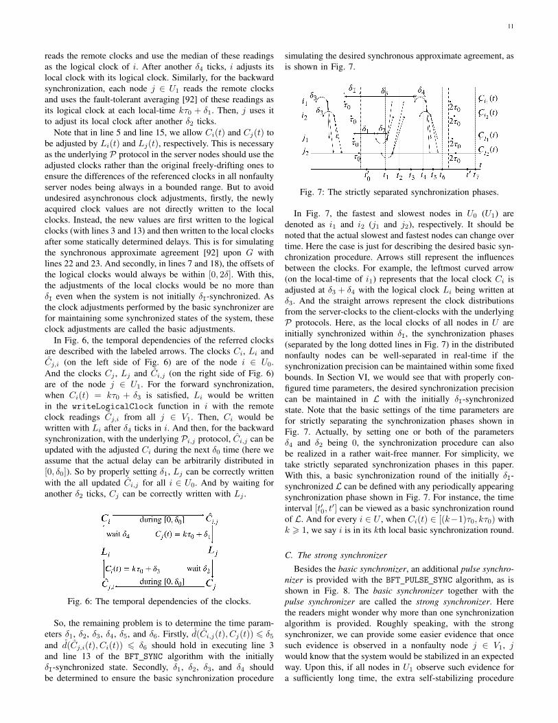
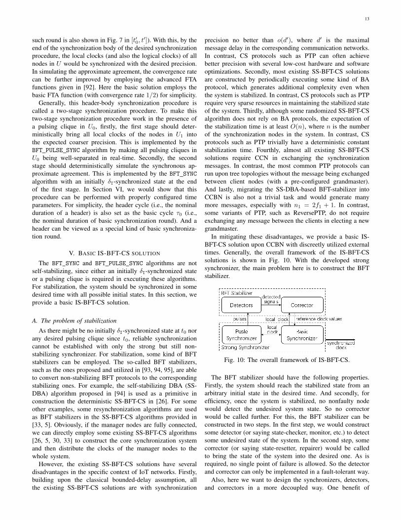