nearly time optimal stabilizing patchy feedbacks

arX

iv:m

ath/

0512

531v

1 [m

ath.

CA

] 22

Dec

200

5 Nearly Time Optimal Stabilizing Patchy Feedbacks

Fabio Ancona(∗) and Alberto Bressan(∗∗)

(*) Dipartimento di Matematica and C.I.R.A.M., Universita di Bologna,Piazza Porta S. Donato 5, Bologna 40127, Italy.e-mail: [email protected]

(*) Dept. of Mathematics, Penn State University, University Park, Pa. 16802, U.S.A.e-mail: [email protected]

November 2005

Abstract. We consider the time optimal stabilization problem for a nonlinear control systemx = f(x, u). Let τ(y) be the minimum time needed to steer the system from the state y ∈ R

n tothe origin, and call A(T ) the set of initial states that can be steered to the origin in time τ(y) ≤ T .Given any ε > 0, in this paper we construct a patchy feedback u = U(x) such that every solution ofx = f(x, U(x)), x(0) = y ∈ A(T ) reaches an ε-neighborhood of the origin within time τ(y) + ε.

Keywords and Phrases. Time optimal stabilization, Discontinuous feedback control, robustness.1991 AMS-Subject Classification. 34 A, 34 D, 49 E, 93 D.

http://arXiv.org/abs/math/0512531v1

Nearly Time Optimal Patchy Feedbacks 1

1 - Introduction

Consider an optimization problem for a nonlinear control system of the form

x = f(x, u) u(t) ∈ U , (1.1)

where x ∈ Rn describes the state of the system, the upper dot denotes a derivative w.r.t. time,

while U ⊂ Rm is the set of admissible control values. A central issue in the theory of optimal

control is the existence of a feedback control u = U(x) such that all trajectories of

x = f(x, U(x)

)(1.2)

are optimal, for a given performance criterion. In most cases, the optimal feedback law u = U(x) isnot continuous. As shown in Example 1.1 in [27] or Example 2 in [10], even near-optimal feedbacklaws can usually be found only within a class of discontinuous functions.

Therefore, it is essential to provide suitable definitions of “generalized solutions” for discontin-uous ODE’s. In particular, we recall the concept of “sample-and-hold” solutions and Euler solutions(limits of sample-and-hold solutions), which were successfully implemented both within the contextof stabilization problems [16, 31, 34] and of near-optimal feedbacks [17, 19, 27] (see also [26] fora discussion of further definitions of generalized solutions relevant for optimization problems). Adrawback of this approach is that, as illustrated by Example 5.3 and Example 5.4 in [30], arbitrarydiscontinuous feedback can generate too many trajectories, some of which fail to be optimal. Infact, Example 5.3 in [30] shows that the set of Caratheodory solutions of the optimal closed-loopequation (1.2) contains, in addition to all optimal trajectories, some other arcs that are not optimal.Moreover, Example 5.4 in [30] exhibits an optimal control problem in which the optimal trajectoriesare Euler solutions, but the closed-loop equation (1.2) has many other Euler solutions which are notoptimal.

A different strategy, proposed by Piccoli [28] and Sussmann [35], takes as primary object ofinvestigation an optimal “synthesis” which is just a collection of optimal trajectories not necessarilyarising from a feedback control. A general notion of regular synthesis is discussed in [30] where asufficiency theorem for optimal synthesis is proved. The existence and the structure of an optimalsynthesis has been the subject of a large body of literature on nonlinear control. At present, detailedresults are known for time optimal planar systems of the form

x = f(x) + g(x)u u ∈ [−1, 1] , x ∈ R2 ,

see [9] and the references therein. For more general classes of optimal control problems, or in higherspace dimensions, the construction of an optimal synthesis faces severe difficulties. On one hand, theoptimal synthesis can have an extremely complicated structure, and only few regularity results arepresently known (see [23]). Already for systems in two space dimensions, an accurate description ofall generic singularities of a time optimal synthesis involves the classification of eighteen topologicalequivalence classes of singular points [28, 29]. In higher dimensions, an even larger number ofdifferent singularities arises, and the optimal synthesis can exhibit pathological behavior such as thethe famous “Fuller phenomenon” (see [25], [36]), where every optimal control has an infinite numberof switchings. On the other hand, even in cases where a regular synthesis exists, the performanceachieved by the optimal synthesis may not be robust. In other words, small perturbations cangreatly affect the behavior of the synthesis (e.g. see Example 5.3 in [30]).

2 F. Ancona and A. Bressan

Because of the difficulties faced in the construction of an optimal syntheses, it seems naturalto slightly relax our requirements, and look for nearly-optimal feedbacks instead. This is indeedthe main purpose of the present paper. Within this wider class, one can hope to find a feedbacklaw whose discontinuities are sufficiently ”tame”, providing the existence of trajectories in the usualCaratheodory sense, all of which are “almost optimal”. Moreover, the new feedback laws will havea simpler structure and better robustness properties than a regular synthesis.

For sake of definiteness, we shall study the problem of steering the system (1.1) from any initialstate y ∈ R

n to the origin in minimum time, under the basic assumptions

(H) The set U ⊂ Rm of admissible control values is bounded. Moreover, the function f : R

n×Rm 7→

Rn is twice continuously differentiable and has sublinear growth:

∣∣f(x, u)∣∣ ≤ c

(1 + |x|

)for all u ∈ U . (1.3)

For y ∈ Rn, call T (y) the minimum time needed to steer the system from the state y ∈ R

n to theorigin, i.e. set

T (y).= inf

t ≥ 0 ; there exists some trajectory x(·) of (1.1)

that satisfies x(0) = y, x(t) = 0

.(1.4)

Roughly speaking, our main theorem states the following. If we relax a bit the optimality require-ments, asking that every initial state y be steered inside an ε-neighborhood of the origin within timeT (y) + ε, then this can be accomplished by a patchy feedback, for any fixed ε > 0.

Patchy feedback controls were first introduced in [1] in order to study asymptotic stabilizationproblems. They have a particularly simple structure, being piecewise constant in the state space R

n.Moreover, the Caratheodory solutions of the corresponding Cauchy problems (1.2) enjoy importantrobustness properties [2, 3, 4], which are particularly relevant in many practical situations. Indeed,one of the main reasons for using a state feedback is precisely the fact that open loop controls areusually very sensitive to disturbances. In particular, we have shown in [2] that a patchy feedbackis “fully robust” with respect to perturbation of the external dynamics, and to measurement er-rors having sufficiently small total variation so to avoid the chattering behavior that may arise atdiscontinuity points.

We recall here the main definitions (see [1]):

Definition 1.1. By a patch we mean a pair(Ω, g

)where Ω ⊂ R

n is an open domain with smooth

boundary ∂Ω, and g is a smooth vector field defined on a neighborhood of the closure Ω of Ω, whichpoints strictly inward at each boundary point x ∈ ∂Ω.

Calling n(x) the outer normal at the boundary point x, we thus require

⟨g(x), n(x)

⟩< 0 for all x ∈ ∂Ω. (1.5)

Definition 1.2. We say that g : Ω 7→ Rn is a patchy vector field on the open domain Ω if there

exists a family of patches(Ωα, gα); α ∈ A

such that

- A is a totally ordered set of indices,

- the open sets Ωα form a locally finite covering of Ω,


- the vector field g can be written in the form

g(x) = gα(x) if x ∈ Ωα \⋃

β>α

Ωβ. (1.6)

We shall occasionally adopt the longer notation(Ω, g, (Ωα, gα)

α∈A

)to indicate a patchy vector

field, specifying both the domain and the single patches.

By settingα∗(x)

.= max

α ∈ A ; x ∈ Ωα

, (1.7)

we can write (1.6) in the equivalent form

g(x) = gα∗(x)

(x) for all x ∈ Ω. (1.8)

Remark 1.1. Notice that the patches (Ωα, gα) are not uniquely determined by a patchy vectorfield (Ω, g). Indeed, whenever α < β, by (1.6) the values of gα on the set Ωα ∩ Ωβ are irrelevant.Therefore, if the open sets Ωα form a locally finite covering of Ω and we assume that, for eachα ∈ A, the vector field gα satisfies (1.5) at every point x ∈ ∂Ωα \ ⋃

β>α Ωβ , then the vector field g

defined according with (1.6) is again a patchy vector field. To see this, it suffices to construct vectorfields gα (defined on a neighborhood of Ωα as gα) which satisfy the inward pointing property (1.5)at every point x ∈ ∂Ωα and such that gα = gα on Ωα \ ⋃

β>α Ωβ (cfr.[1, Remark 2.1]). In fact,with the same arguments one deduces that, to guarantee that a vector field g defined on an opendomain Ω according with (1.6) be a patchy vector field, it is sufficient to require that each vectorfield gα satisfy (1.5) at every point x ∈ ∂Ωα \

(( ⋃β>α Ωβ

)∪ ∂Ω

).

If g is a patchy vector field, the differential equation

x = g(x) (1.9)

has several useful properties. In particular, in [1] it was proved that the set of Caratheodory solutionsof (1.8) is closed (in the topology of uniform convergence) but possibly not connected. Moreover,given an initial condition

x(t0) = x0, (1.10)

the Cauchy problem (1.9)-(1.10) has at least one forward solution, and at most one backward so-lution, in the Caratheodory sense. For every Caratheodory solution x = x(t) of (1.9), the mapt 7→ α∗(x(t)) is left continuous and non-decreasing.

Remark 1.2. In some situations it is useful to adopt a more general definition of patchy vectorfield than the one formulated above. Indeed, one can consider patches (Ωα, gα) where the domainΩα has a piecewise smooth boundary (see [3]). In this case, the inward-pointing condition (1.5) canbe expressed requiring that

g(x) ∈

TΩ(x) (1.11)

where

TΩ(x) denotes the interior of the tangent cone to Ω at the point x, defined by

TΩ(x).=

v ∈ R

n : lim inft↓0

d(x + tv, Ω

)

t= 0

. (1.12)


Clearly, at any regular point x ∈ ∂Ω, the interior of the tangent cone TΩ(x) is precisely the set ofall vectors v ∈ R

n that satisfy⟨v, n(x)

⟩< 0 and hence (1.11) coincides with the inward-pointing

condition (1.5). One can easily see that all the results concerning patchy vector fields establishedin [1, 2] remain true within this more general formulation.

Definition 1.3. Let(Ω, g, (Ωα, gα)

α∈A

)be a patchy vector field. Assume that there exist control

values vα ∈ U such that, for each α ∈ A, there holds

gα(x) = f(x, vα) ∀ x ∈ Dα.= Ωα \

⋃

β>α

Ωβ . (1.13)

Then, the piecewise constant map

U(x).= vα if x ∈ Dα (1.14)

is called a patchy feedback control on Ω, and referred to as(Ω, U, (Ωα, vα)

α∈A

).

Remark 1.3. By Definitions 1.2 and 1.3, the vector field

g(x) = f(x, U(x)

)

defined in connection with a given patchy feedback(Ω, U, (Ωα, vα)

α∈A

)is precisely the patchy

vector field(Ω, g, (Ωα, gα)

α∈A

)associated with a family of fields

gα : α ∈ A

satisfying (1.5)

Notice that, recalling the notation (1.7), for all x ∈ Ω we have

U(x) = vα∗(x) . (1.15)

As observed in Remark 1.1, the values of the vector fields f(x, vα) on the set Ωα ∩Ωβ are irrelevantwhenever α < β, and it is not necessary that f(x, vα) satisfy the inward-pointing condition (1.5)at the points of ∂Ωα ∩

( ⋃β>α Ωβ

). Moreover, all the properties of a patchy feedback continue to

hold even in the case where we assume that the inward-pointing condition (1.5) fails to be satisfiedat the points of (∂Ωα ∩ Σ) \ ⋃

β>α Ωβ , for some region Σ of the boundary ∂Ω. Clearly, in this caseevery Caratheodory trajectory of the patchy vector field g can eventually reach the boundary ∂Ωonly crossing points of Σ.

To state our main results, we first need to relax the minimum time problem. Call U the familyof admissible control functions, i.e. all measurable functions t 7→ u(t), t ≥ 0, with u(t) ∈ U almosteverywhere. For y ∈ R

n and u ∈ U , we denote by t 7→ x(t; y, u) the solution of the Cauchy problem

x(t) = f(x(t), u(t)

), x(0) = y . (1.16)

The global existence and the uniqueness of this solution are guaranteed by the assumptions (H).Now fix ε > 0 arbitrarily small and define the penalization function

ϕε(x).=

|x|2ε2 − |x|2 if |x| < ε ,

∞ if |x| ≥ ε .

(1.17)


Consider the following ε-approximate minimization problem:

inft≥0 ; u∈U

t + ϕε

(x(t; y, u)

). (1.18)

We denote this infimum by V (y), for every y ∈ Rn, and refer to y 7→ V (y) ∈ [0,∞] as the value

function for (1.18). Observe that V (y) ≤ T (y). Hence, for a fixed time T > 0, the set of points thatcan be steered to the origin within time T is contained in the sub-level set

ΛT.=

y ∈ R

n ; V (y) ≤ T

. (1.19)

With the above notations, our main result can be stated as follows.

Theorem 1. Let the assumptions (H) hold and, given ε > 0, T > 0, let ΛT be the sub-level setdefined in (1.19) in connection with the value function V for (1.18). Then, there exists a patchyfeedback control u = U(x), defined on a neighborhood of

ΛT,ε.=

y ∈ R

n ; V (y) ≤ T ; |y| ≥ ε, (1.20)

such that, for each y ∈ ΛT,ε, every Caratheodory solution of

x = f(x, U(x)

), x(0) = y (1.21)

reaches the ballBε

.=

x ∈ R

n ; |x| ≤ ε

within time V (y) + ε.

The assumptions (H) are very general. They do not even imply the existence of optimal controls,even for the relaxed problem (1.18). We recall that the standard existence theory requires theadditional assumptions

(H′) The set U ⊂ Rm of admissible control values is compact. For every x ∈ R

n, the set of velocitiesf(x, u) ; u ∈ U

is convex.

If both (H) and (H′) hold, then the infimum in (1.4) and in (1.18) are actually attained(e.g. cfr. [14]). Moreover, the minimum time function T : R

n 7→ [0,∞] is lower semicontinuous.This fact is a well known consequence of the closure property of the graph of the set valued mapS : [0, ∞)×R

n Rn defined by S(t, y)

.=

x(t; y, u) ; u ∈ U

. Because of the lower semicontinuity

of the minimum time function, and by (1.3), it follows that, for every τ ≥ 0, the attainable set

A(τ).=

y ∈ R

n ; T (y) ≤ τ

(1.22)

is compact. Since V (y) ≤ T (y) for all y ∈ Rn, from Theorem 1 one thus obtains

Corollary. Let the assumptions (H) and (H′) hold, and let ε > 0, τ > 0 be given. Then there existsa patchy feedback control u = U(x), defined on a neighborhood of the set

Aε(τ).=

y ∈ R

n ; T (y) ≤ τ ; |y| ≥ ε

, (1.23)


such that, for each y ∈ Aε(τ), every Caratheodory solution of (1.21) reaches the ball Bε withintime T (y) + ε.

In all previous papers [1, 2, 3] the construction of a stabilizing patchy feedback did not makeany use of a control-Lyapunov function for (1.1). Instead, the feedback law was obtained by patchingtogether a finite number of open-loop controls. We remark that a straightforward adaptation of thisstrategy would not work here. Indeed, let ε > 0 be given. As in [1], we can then cover the set Aε(τ)with finitely many tubes Ω1, . . . , ΩN and construct a patchy feedback u = Uα(x) steering each pointy ∈ Ωα inside the ball Bε within time T (y) + ε. However, we cannot guarantee that the patchyfeedback

u(x) = Uα∗(x) α∗(x).= max α ; x ∈ Ωα (1.24)

is nearly-optimal (see Fig.1). Indeed, call Tα(y) the time taken by the control Uα to steer the pointy ∈ Ωα inside Bε. Let t 7→ x(t) be a trajectory of the patchy feedback (1.24), with x(0) = y,x(τ) ∈ Bε. Assume α∗(t) = α for t ∈ ]tα−1 , tα] . The near-optimality of each feedback impliesTα(x) ≤ T (x) + ε for every x. Moreover

Tα(x(tα−1)) − Tα(x(tα)) = (tα − tα−1) .

Unfortunately, from the above inequalities one can only deduce

T (x(tα−1)) − T (x(tα)) ≥ (tα − tα−1) − ε .

and hence τ ≤ T (y) + Nε . This is a useless information, because the number N of tubes may wellapproach infinity as ε → 0.

3Ω

2Ω

1Ω

figure 1


To overcome this problem, in the present paper we perform an entirely different constructionof the patchy feedback. As starting point, instead of open-loop controls, we use the value function

V for the problem (1.18), together with a piecewise quadratic approximation V . This has the form

V (x) = minj

Vj(x) , Vj(x) = aj + bj · x + c |x|2.

and satisfies V (x) ≤ V (x)+ ε for each point x. The result will be achieved by constructing a patchyfeedback such that

d

dtV

(x(t)

)= ∇V

(x(t)

)· f

(x(t), u(x(t)

)≤ ε

at a.e. time t.

2 - Preliminary results

Throughout the paper, by B(x, r) we denote the closed ball centered at x with radius r, and

set Br.= B(0, r). The closure, the interior and the boundary of a set Ω are written as Ω,

Ω and ∂Ω,respectively, while diam(Ω) denotes the diameter of a bounded set Ω. The distance of a point xfrom a set Ω is denoted by dΩ(x), while dΩ(E)

.= infx∈E dΩ(x) denotes the distance between two

sets Ω, E. The number of elements of a finite set J is denoted by |J |.We begin by observing that the infimum in (1.18) provides an upper bound for the time needed

to steer the system (1.1) from y to the ball Bε. Hence, for every T ≥ 0, the sub-level set ΛT of thevalue function V for (1.18) is contained in the set of points that can be steered to the ball Bε withintime T . On the other hand, notice that the scalar Cauchy problem

z = c (1 + z) , z(0) = ε , (2.1)

has solution

z(t) = (1 + ε)ect − 1 . (2.2)

Therefore, because of (1.3), a comparison argument yields

ΛT ⊆ Bz(T ) , (2.3)

for every T ≥ 0.

In connection with the relaxed minimization problem (1.18), we now show that the value func-tion V is Lipschitz continuous on ΛT and locally semiconcave, that is, for any x0, there exists aconstant c0 > 0 such that there holds

V (x1) + V (x2) − 2V

(x1 + x2

2

)≤ c0

∣∣x1 − x2

∣∣2 (2.4)

for all x1, x2 in a neighborhood of x0. We refer to [14] for the definition and properties of semiconcavefunctions.


Lemma 1. With the assumptions (H), for any fixed ε, T > 0 the restriction of the value function Vfor (1.18) to the sublevel set ΛT is Lipschitz continuous and locally semiconcave. Indeed, there existsa positive constant λ such that, for every point y0 ∈ ΛT where V is differentiable, there holds

V (y) ≤ V (y0) +⟨∇V (y0), y − y0

⟩+ λ |y − y0|2 ∀ y ∈ ΛT . (2.5)

Proof.1. First observe that, since we are only proving something about the value function V for (1.18),it is not restrictive to assume that the additional hypotheses (H′) hold. Indeed, allowing the setof controls to range in the closure of U does not affect the value function. Moreover, if the sets ofvelocites

f(x, u) ; u ∈ U

are not convex, we can replace the original system (1.1) by a chattering

one (see [Be]), such that the problem (1.18) yields exactly the same value function. This in particularimplies that the value function V is lower semicontinuous and that the sub-level set (1.19) is compact.

2. Next, observe that, since the function f is twice continuously differentiable and the sets ΛT , Uare compact, by standard differentiability properties of the trajectories of a control system (1.1),there holds

supt∈[0,T ], y∈ΛT

u∈U

∣∣∣∣∂

∂yx(t; y, u)

∣∣∣∣ ≤ expT ‖Dxf‖L∞(ΛT )

.= M1 , (2.6)

supt∈[0,T ], y∈ΛT

u∈U

∣∣∣∣∂2

∂y2x(t; y, u)

∣∣∣∣ ≤[M1

(1 + TM3

1 ‖D2xf‖L∞(ΛT )

)] .= M2 , (2.7)

where

‖Dxf‖L∞(ΛT ).= sup

x∈ΛT , u∈U

∣∣∣∣∂

∂xf(x, u)

∣∣∣∣ < ∞ ,

‖D2xf‖L∞(ΛT )

.= sup

x∈ΛT , u∈U

∣∣∣∣∂2

∂x2f(x, u)

∣∣∣∣ < ∞ ,

(2.8)

provide a bound on the first and second partial derivatives of f w.r.t. the x-variable, over the set ΛT .Then, because of (2.6), there exists a constant c1 such that

∣∣x(t; y2, u) − x(t; y1, u)∣∣ ≤ c1|y2 − y1| ∀ t ∈ [0, T ], y1, y2 ∈ ΛT , u ∈ U . (2.9)

3. Given y0 ∈ ΛT , by the previous assumptions at point 1 there exists an optimal control u0 ∈ U ,and a time t0, such that

t0 + ϕε

(x(t0; y0, u0)

)= V (y0) ≤ T . (2.10)

This, by definition (1.17) of ϕε , of course implies

t0 ≤ T ,∣∣x(t0; y0, u0)

∣∣ ≤ ε

√T

1 + T. (2.11)


Hence, using (2.11) together with (2.9), we find that there exists some constant δ > 0, dependingonly on ε, T, and on c1, but not on the point y0 ∈ ΛT , such that

∣∣x(t0; y, u0)∣∣ ≤ ε

√2T + 1

2(1 + T )∀ y ∈ B(y0, δ) ∩ ΛT . (2.12)

Observe now that, since V (y) is the infimum in (1.18), there holds

V (y) ≤ V 0(y).= t0 + ϕε

(x(t0; y, u0)

)∀ y . (2.13)

Because of (2.12), the map y 7→ V 0(y) defined in (2.13) is twice continuously differentiable at everypoint of B(y0, δ) ∩ ΛT . Hence, since (2.10) implies V 0(y0) = V (y0), there holds

V 0(y) ≤ V (y0) +⟨∇V 0(y0), y − y0

⟩+ λ0

∣∣y − y0

∣∣2 ∀ y ∈ B(y0, δ) ∩ ΛT , (2.14)

withλ0

.= sup

η∈B(y0,δ)∩ΛT

∣∣D2V 0(η)∣∣ .

The gradient of the function V 0 is computed by

∇V 0(y) = ∇ϕε

(x(t0; y, u0)

)· ∂

∂yx(t0; y, u0) .

Thus, relying on (2.6), (2.12), and setting

M0.= sup

t∈[0,T ], y∈ΛT

u∈U

∣∣x(t; y, u)∣∣ , (2.15)

we obtain

∣∣∇V 0(y)∣∣ ≤ 2ε2

∣∣x(t0; y, u0)∣∣

(ε2 −

∣∣x(t0; y, u0)∣∣2

)2 · M1 ≤ 8(1 + T )2M0M1

ε2

.= c2 ∀ y ∈ B(y0, δ) ∩ ΛT .

(2.16)With similar computations, using (2.7), (2.12), we find that a bound on the second derivative of V 0

is provided by

∣∣D2V 0(y)∣∣ ≤

∣∣D2ϕε

(x(t0; y, u0)

)∣∣ ·∣∣∣∣

∂

∂yx(t; y, u)

∣∣∣∣ +∣∣∇ϕε

(x(t0; y, u0)

)∣∣ ·∣∣∣∣

∂2

∂y2x(t; y, u)

∣∣∣∣

≤[8(1 + T )2M1

ε2+

64(1 + T )3M20 M1

ε4+

8(1 + T )2M0M2

ε2

].= c3 ∀ y ∈ B(y0, δ) ∩ ΛT .

(2.17)Notice that the constants c2, c3 depend only on ε, T, and on the function f , but not on the pointy0 ∈ ΛT . Then, (2.13), (2.14), together with (2.16), (2.17) yield

V (y) ≤ V (y0) +(c2 + δ c3)

∣∣y − y0

∣∣ ∀ y ∈ B(y0, δ) ∩ ΛT , ∀ y0 ∈ ΛT , (2.18)


which, in turn, implies

y1, y2 ∈ ΛT ,∣∣y1 − y2| < δ =⇒

∣∣V (y1) − V (y2)∣∣ ≤

(c2 + δ c3) ·

∣∣y1 − y2| . (2.19)

Since the set ΛT is compact, we deduce from (2.19) that the map V is (globally) Lipschitz continuouson ΛT .

4. Given y0 ∈ ΛT , in connection with the constants λ0, δ, c2 introduced at point 3 choose

λ > max

λ0,

Lip(V ) + c2

δ

,

and observe that, because of (2.16), there holds

⟨∇V 0(y0), y − y0

⟩+ λ

∣∣y − y0

∣∣2 ≥ (−c2 + λ δ)∣∣y − y0

∣∣

≥ Lip(V ) ·∣∣y − y0

∣∣∀ y ∈ ΛT \ B(y0, δ) . (2.20)

Thus, (2.13), (2.14), together with (2.20), yield

V (y) ≤ V (y0) +⟨∇V 0(y0), y − y0

⟩+ λ

∣∣y − y0

∣∣2 ∀ y ∈ ΛT . (2.21)

5. Fix ρ > 0. By the above arguments there exist a positive constant λ = λρ so that, for everyfixed y0 ∈ ΛT+ρ, the estimate (2.21) holds for all y ∈ ΛT+ρ. Next, given x0 ∈ ΛT , choose δ0 so

that B(x0, δ0) ⊂ ΛT+ρ. Then, for any y1, y2 ∈ B(x0, δ0) ∩ ΛT , one has y1+y2

2 ∈ ΛT+ρ. Hence,

applying (2.21) for y = yi, i = 1, 2, and y0 = y1+y2

2 , and summing up the corresponding inequalities,since y1 − y0 = y0 − y2 we obtain

V (y1) + V (y2) ≤ 2V

(y1 + y2

2

)+ λ

[∣∣y1 − y0

∣∣2 +∣∣y2 − y0

∣∣2]≤ 2V

(y1 + y2

2

)+ λ

∣∣y1 − y2

∣∣2 ,

which shows that the estimate (2.4) is verified, with c0 = λ, for all y1, y2 ∈ ΛT in the ball B(x0, δ0).Therefore, the map V is locally semiconcave on ΛT .

6. To conclude the proof of the lemma, consider a point y0 ∈ ΛT where V is differentiable, andobserve that, by (2.21), one has

⟨∇V (y0) −∇V 0(y0),

y − y0

|y − y0|⟩≤ λ

[|y − y0| +

o(|y − y0|)|y − y0|

](2.22)

for all y ∈ ΛT . Thus, taking yσ.= y0 + σ ∇V (y0)−∇V 0(y0)

|∇V (y0)−∇V 0(y0)|, σ > 0 from (2.22) we deduce

∣∣∇V (y0) −∇V 0(y0)∣∣ ≤ λ

[σ +

o(σ)

σ

]∀ σ > 0 . (2.23)

By letting σ → 0 in (2.23) we obtain ∇V 0(y0) = ∇V (y0) which, together with (2.21), yields (2.5),completing the proof of the lemma.


We next show that the value function V enjoys an infinitesimal decrease property at every pointwhere it is differentiable, which is expressed in terms of an Hamilton-Jacobi inequality.

Lemma 2. With the assumptions (H), given ε, T > 0, let V be the value function for (1.18). Then,there exists 0 < ε0 < ε such that, letting ΛT,ε0 be the set defined in (1.20), for each y ∈ ΛT,ε0 atwhich V is differentiable there holds

infv∈U

⟨∇V (y), f(y, v)

⟩+ 1 ≤ 0 . (2.24)

Proof. Given ε, T > 0, set

ε0.= ε

√4T + 1

2(1 + 2T ), ε′0

.= ε

√2T

1 + 2T, (2.25)

τ0.= c−1 ln

(ε0 + 1

ε′0 + 1

), (2.26)

where c denotes the constant in (1.3), and observe that, by definition (1.17) of ϕε , one has

ϕε(x) ≥ 2T whenever |x| ≥ ε′0 . (2.27)

Then, recalling that (2.2) provides the solution to the scalar Cauchy problem (2.1), by a comparisonargument, and because of (1.3), we deduce that

|y| ≥ ε0 =⇒∣∣x(t; y, u)

∣∣ ≥ ε′0 ∀ t ∈ [0, τ0], u ∈ U . (2.28)

Hence, (2.27) together with (2.28), yields

t + ϕε

(x(t; y, u)

)≥ 2T ∀ t ∈ [0, τ0], |y| ≥ ε0, u ∈ U . (2.29)

¿From (2.29) we deduce that, for every y ∈ ΛT,ε0 , the value function for (1.18) satisfies

V (y) = inft>τ0 ; u∈U

t + ϕε

(x(t; y, u)

)> τ0 . (2.30)

Thus, we reach the conclusion of the Lemma observing that by standard arguments in controltheory (e.g. see [14]) one can show that the value function for (2.30) satisfies the Hamilton-Jacobyinequality (2.24) at every point where V is differentiable.

Remark 2.1. Notice that, in the proof of Theorem 1, we shall only need to have at a disposal avalue function V satisfying the conclusions of Lemma 1 and Lemma 2.

We state now two technical results which will be useful later in the construction of an almosttime optimal patchy feedback. We shall provide a proof of them in the Appendix at the end ofthe paper. Throughout the following, for any given subset C of a sphere S, we let ∂

SC denote the

boundary of C relative to the topology of S.


Lemma 3. Given r0 > 0, let S be a sphere with radius r ≥ r0, and let g be a bounded,Lipschitz continuous vector field which points strictly inward at the points of a closed set C ⊂ Sthat has a piecewise smooth relative boundary ∂

SC. More precisely, letting nS(y) denote the unit

outer normal to S at the point y, assume that⟨nS(y), g(y)

⟩≤ −c ∀ y ∈ C , (2.31)

for some constant c > 0. Denote by t 7→ x(t, y) the solution of the Cauchy problem x = g(x),x(0) = y. Then there exists ε > 0, depending only on r0, c, ‖g‖L∞ , and on the Lipschitz constantLip(g) of g, such that the following holds. Define

Γε(C).=

x(τ, y) ; y ∈ B(C, ε) ∩ S , d

C

2(y) − ε2 < τ ≤ 0

. (2.32)

Then the vector field g is transversal to the boundary of Γε.= Γε(C). Indeed, it points strictly inward

on the set

∂−Γε.=

x(d

C

2(y) − ε2, y) ; y ∈

B(C, ε) ∩ S

(2.33)

and strictly outward on the set∂+ Γε

.= ∂ Γε ∩ S . (2.34)

The lens-shaped domain (2.32) provides the basic building block for the construction of thepatchy feedback produced in the next section. In some situations it will be necessary to restrict suchdomains cutting them along hyperplanes in order to preserve the (almost) time-optimality propertyof the feedback law. The next lemma provides an a-priori lower bound on the distance between theupper boundary of a collection of such domains and the union of spheres around which the domainsare cosntructed.

π−

π−

S

(CΓ

CΓ (C )

C

S

)

ππ+

figure 2

Lemma 4. Given 0 < r0 < r′0, let B1, . . . , Bν be a finite collection of balls with surfaces S1, . . . , Sν ,having radii r1, . . . , rν ∈ [r0, r′0], and satisfying

Si ∩ν⋃

j=1

Bj 6= ∅ ,

Si \ν⋃

j=1

Bj 6= ∅ ,

∀ i = 1, . . . , ν . (2.35)


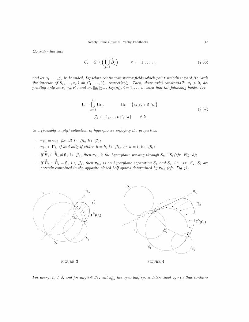
Consider the sets

Ci.= Si \

( ν⋃

j=1

Bj

)∀ i = 1, . . . , ν , (2.36)

and let g1, . . . , gν be bounded, Lipschitz continuous vector fields which point strictly inward (towardsthe interior of S1, . . . , Sν) on C1, . . . , Cν , respectively. Then, there exist constants ε′, c4 > 0, de-pending only on ν, r0, r

′0, and on ‖gi‖L∞ , Lip(gi), i = 1, . . . , ν, such that the following holds. Let

Π =ν⋃

k=1

Πk , Πk.=

πk,i ; i ∈ Jk

,

Jk ⊂ 1, . . . , ν \ k ∀ k ,

(2.37)

be a (possibly empty) collection of hyperplanes enjoying the properties:

– πk,i = πi,k for all i ∈ Jk, k ∈ Ji ;

– πk,i ∈ Πh if and only if either h = k, i ∈ Jh, or h = i, k ∈ Jh ;

– if

Bk ∩

Bi 6= ∅ , i ∈ Jk, then πk,i is the hyperplane passing through Sk ∩ Si (cfr. Fig. 3);

– if

Bk ∩

Bi = ∅ , i ∈ Jk, then πk,i is an hyperplane separating Sk and Si, i.e. s.t. Sk, Si areentirely contained in the opposite closed half spaces determined by πk,i (cfr. Fig 4) .

Si

k)(CΓJ k

Sl

k)(CJ k

πk,i−

πk,i−

Sk

CkSj

Sj

Sk

Ck

Si k,iπ

Γ

k,iπ

figure 3 figure 4

For every Jk 6= ∅, and for any i ∈ Jk, call π−k,i the open half space determined by πk,i that contains


Ck \ ∂Sk

Ck. Then, setting

ΓJk

ε′

.= Γ

Jk

ε′(Ck)

.=

Γε′(Ck) ∩⋂

i∈Jk

π−k,i if Jk 6= ∅ ,

Γε′(Ck) otherwise ,

k = 1, . . . , ν , (2.38)

C.=

ν⋃

k=1

Ck , G .=

ν⋃

k=1

ΓJk

ε′, (2.39)

∂−G .= ∂ G \

ν⋃

k=1

Bk , (2.40)

one has

dC

(∂−G

)≥ c4 . (2.41)

G

kJ

(C )Γ k

CCk

−

figure 5

3 - Proof of the theorem

The proof will be given in several steps.

1. Given ε, T > 0 (ε < min1, T ), fix some constant T ′ > T + 1, and observe that by Lemma 1the value function V for (1.18) is Lipschitz continuous on ΛT ′

.=

y ∈ R

n ; V (y) ≤ T ′. Hence, by


Rademacher’s theorem V is differentiable a.e. in ΛT ′ . Then, letting λ > 0 be the constants providedby Lemma 1 in connection with the set ΛT ′ , for each y ∈ ΛT ′ at which V is differentiable define aquadratic function V y setting

V y(x).= V (y) + ∇V (y) · (x − y) + (1 + λ) |x − y|2 . (3.1)

Notice that, because of (2.5), there holds

V (x) + |x − y|2 ≤ V y(x) ∀ x ∈ ΛT ′ . (3.2)

Moreover, according with Lemma 2, there exists some constant ε0 > 0 so that, given a constant

0 < ε1 <ε

4T ′, (3.3)

for every y ∈ ΛT ′, ε0

.=

y ∈ ΛT ′ ; |y| ≥ ε0

where V is differentiable we can choose a control

value vy ∈ U such that ⟨∇V (y), f(y, vy)

⟩< −1 + ε1 . (3.4)

Choose the constant ε0 so that, setting

ε′0.= ε

√4T ′ + 1

2(1 + 2T ′), ε′′0

.= ε

√2T ′

1 + 2T ′,

τ0.= c−1 ln

(ε′0 + 1

ε′′0 + 1

),

(3.5)

where c denotes the constant in (1.3), there holds

ε0 < min

ε

4, ε′0

,

ε20

ε2 − ε20

<τ0

2. (3.6)

Notice that, by definition (1.17) of ϕε, and because of (3.6), the value function V for (1.18) satisfies

V (x) ≤ ε20

ε2 − ε20

<τ0

2∀ x ∈ Bε0 . (3.7)

Next, choose some other constant

L′ > L.= diam(ΛT ′) +

√nLip(V ) +

√n (Lip(V ))2 + 4T ′(1 + λ) , (3.8)

where Lip(V ) denotes the Lipschitz constant of V on ΛT ′ . Hence, since the assumptions (H) implythe Lipschitz continuity in x of the function f(x, u) on the compact set BL′×U, uniformly for u ∈ U,and because also ∇V y is Lipschitz continuous with a Lipschitz constant independent on y ∈ ΛT ′ ,there will be some constant c5 > 0 (depending only on L′) such that

∣∣⟨∇V y(x1), f(x1, u)⟩−

⟨∇V y(x2), f(x2, u)

⟩∣∣ ≤ c5 ·∣∣x1 − x2

∣∣∣∣f(x1, u) − f(x2, u)

∣∣ ≤ c5 ·∣∣x1 − x2

∣∣∀ x1, x2 ∈ BL′ , u ∈ U . (3.9)


Then, settingc6

.=

√n Lip(V ) + 4(1 + λ)diam(ΛT ′) , (3.10)

and choosing ε2 > 0 so that

ε2 < min

√ε

3,

ε1

8c5c6,

√τ0

2,

T ′ − T

1 + Lip(V ), L′ − L

, (3.11)

we deduce from (3.4), (3.9) that, for every y ∈ ΛT ′, ε0 where V is differentiable there holds

⟨∇V y(x), f(x, vy)

⟩< −1 + 2ε1 ∀ x ∈ B(y, 2ε2) ∩ BL′ . (3.12)

2. By the Lipschitz continuity of V on the set ΛT ′ it follows that, for each y ∈ ΛT ′, ε0 at which V isdifferentiable, there holds

∣∣V y(x) − V (x)∣∣ ≤ c7 ·

∣∣x − y∣∣ ∀ x ∈ ΛT ′ ,

for some positive constant c7 . Hence, since the set ΛT ′,ε0 is compact (cfr. point 1 of the proof ofLemma 1), we can cover it with finitely many balls (of sufficiently small radius), centered at pointsof ΛT ′, ε0 where V is differentiable, say y1, . . . , yN , so that, setting

Vi(x).= V yi(x) , 1 ≤ i ≤ N ,

V (x).= min

iVi(x)

∀ x ∈ Rn , (3.13)

there holdsV (x) ≤ V (x) ≤ V (x) + ε2

2 ∀ x ∈ ΛT ′, ε0 . (3.14)

Next, observing that (3.2) implies

Vi(x) > V (x) + ε22 ∀ x ∈ ΛT ′ \ B(yi, ε2) ,

we deduce from (3.14) that

V (x) < Vi(x) ∀ x ∈ ΛT ′, ε0 \ B(yi, ε2) . (3.15)

Relying on (3.15), letting

Pi.=

x ∈ R

n ; Vi(x) = V (x)

, (3.16)

we find thatPi ∩ ΛT ′, ε0 ⊂ B(yi, ε2) , 1 ≤ i ≤ N . (3.17)

Hence, by (3.12), (3.17) we have

⟨∇Vi(x), f(x, vi)

⟩< −1 + 2ε1 ∀ x ∈ B

(Pi, ε2

)∩ ΛT ′, ε0 ∩ BL′ , 1 ≤ i ≤ N , (3.18)

where we have set vi .= vyi (1 ≤ i ≤ N), while (3.2) yields

V (x) ≥ V (x) + |x − yi|2 ∀ x ∈ Pi ∩ ΛT ′ , 1 ≤ i ≤ N . (3.19)


3. The patchy feedback u = U(x) will be constructed looking at the level sets of the function Vdefined in (3.13). To this end, observe first that, because of (3.14), and by the choice (3.11) of ε2,there holds

V (x) < T ′ − Lip(V ) · ε2 ∀ x ∈ ΛT . (3.20)

Moreover, notice that, relying on the definitions (3.1) of V yi and (3.8) of the constant L, one finds

1 ≤ i ≤ N , Vi(x) < T ′ =⇒ |x| ≤ |x − yi| + diam(ΛT ′)

≤ |∇V (yi)| +√|∇V (yi)|2 + 4T ′(1 + λ) + diam(ΛT ′)

≤ √nLip(V ) +

√n (Lip(V ))2 + 4T ′(1 + λ) + diam(ΛT ′)

≤ L ,

(3.21)

which, in turn, by the definition (3.13) of V , and because of (3.14), yields

x ∈ R

n ; V (x) < T ′⊂ ΛT ′ ∩ BL . (3.22)

On the other hand, observe that all level sets of each quadratic function Vi are spheres. Therefore,every level set

Στ.=

x ∈ R

n ; V (x) = τ

τ ≥ τ0 , (3.23)

is contained in a finite union of spheres, and each upper level setx ∈ R

n; V (x) ≥ τ, τ ≥ τ0, is

connected. Moreover, notice that by (3.7), (3.11), (3.14), we derive

max|x|=ε0

V (x) <τ0

2+ ε2

2 ≤ τ0 , (3.24)

and hence we find that x ∈ R

n; V (x) ≥ τ0

∩ Bε0 = ∅ . (3.25)

Thus, setting

T ′′ .= T ′ − Lip(V ) · ε2 , D .

=x ∈ R

n ; τ0 < V (x) < T ′′

, (3.26)

thanks to (3.11), (3.14), (3.20), (3.22), (3.25), we deduce that

ΛT,ε ⊂ B(D, ε2

)⊂ ΛT ′, ε0 ∩ BL . (3.27)

We will establish the theorem by constructing the patchy feedback u = U(x) on the domain D. Noticethat, with the same arguments used in the proof of Lemma 2, by the choice of the constants ε′0, τ0

in (3.5) we find thatV (x) > τ0 ∀ x ∈ ΛT ′ , |x| ≥ ε′0 . (3.28)

Hence, since the definition (3.13) of V implies

V (x) ≤ τ0 ∀ x ∈ Στ0 ,

we deduce from (3.6), (3.28) thatΣτ0 ⊂ Bε′

0⊂ Bε . (3.29)


Next, observe that, since all functions Vi, 1 ≤ i ≤ N , have the same coefficient of the quadraticterm, it follows that, for each couple of indices k 6= i, the set

πk,i.= πi,k

.=

x ∈ R

n ; Vk(x) = Vi(x)

(3.30)

is an hyperplane, and the difference of the gradients ∇Vi(x) −∇Vk(x) is a constant vector on πk,i.Then, letting nk,i denote the unit normal to πk,i, pointing towards the half space

π+k,i

.= π−

i,k.=

x ∈ R

n ; Vk(x) > Vi(x)

, (3.31)

one has∇Vi(x) −∇Vk(x) = −cnk,i ∀ x ∈ πk,i , (3.32)

for some constant c = ck,i ≥ 0. Denote as π−k,i the other half space determined by πk,i, i.e. set

π−k,i

.= π+

i,k.=

x ∈ R

n ; Vk(x) < Vi(x)

. (3.33)

4. The basic step in the construction of U(x) is the following. We shall fix a suitably small timesize ∆t and, in connection with an increasing sequence of times τmm≥0 with the property

∃ p s.t. τm+p > τm + ∆t ∀ m ,

we will construct, for every m ≥ 0, a patchy feedback whose domain contains the region

Dm.=

x ∈ R

n ; τm < V (x) ≤ τm+1

,

so that all the trajectories x(t) of the corresponding closed-loop system (1.2) satisfy

d

dtV

(x(t)

)≤ −1 + 3ε1 for a.e. t ,

and eventually enter the set where V < τm. To this end, fix any τ ∈ [τ0, T′[ and consider the level

set Στ of V . By construction, Στ is contained in the union of finitely many spheres, say Si1 , . . . , Siντ.

Here we denote as Siℓ

.=

x ∈ R

n ; Viℓ(x) = τ

the surface of the ball Biℓ

.=

x ∈ R

n ; Viℓ(x) ≤ τ

.

Notice that, since the definition (3.13) of V implies V (x) < τ for all x ∈

Biℓ, by definition (3.23) it

follows that

Στ =

ντ⋃

ℓ=1

Στ,iℓ, Στ,iℓ

.= Siℓ

\ντ⋃

q=1

Biq, (3.34)

x ∈ R

n ; V (x) < τ

=

ντ⋃

ℓ=1

Biℓ. (3.35)

We can assume that the set of indices Iτ.= i1, . . . , iντ

includes only those indices i ∈ 1, . . . , Nfor which there exists some point x ∈ D satisfying

τ = Vi(x) < Vj(x) ∀ j 6= i.


This means that

Iτ =i ∈ 1, . . . , N ;

(Pi \

⋃

j 6=i

Pj

)∩ Στ 6= ∅

, (3.36)

and, in particular, implies that

Si \⋃

j∈Iτ

Bj 6= ∅ ∀ i ∈ Iτ . (3.37)

Moreover, we may write Στ as the union of ητ connected components Σ1τ , . . . , Σ

ητ

τ , so that setting

Ihτ

.=

i ∈ Iτ ;

(Pi \

⋃

j 6=i

Pj

)∩ Σ

hτ 6= ∅

, (3.38)

there holds

Si ∩⋃

j∈Ihτ

Bj 6= ∅ ∀ i ∈ Ihτ , h = 1, . . . , ητ . (3.39)

Notice also that, by (3.13), (3.23), (3.34), (3.37), every set Στ,i, i ∈ Iτ is nonempty and one has

Στ,i =x ∈ R

n ; Vi(x) = V (x) = τ ∀ i ∈ Iτ , (3.40)

while the definitions (3.30), (3.31), (3.33) imply

πk,i ∩ Sk = πk,i ∩ Si = Sk ∩ Si ,

Στ,k ⊂ πk,i ∪ π−k,i , Στ,i ⊂ πk,i ∪ π+

k,i

∀ k, i ∈ Iτ . (3.41)

Therefore, relying on (3.41) we deduce that, for every pair of indices k, i ∈ Iτ , k 6= i, one of thefollowing two cases occurs:

– if

Bk ∩

Bi 6= ∅ , then πk,i is the hyperplane passing through Sk ∩ Si;

– if

Bk∩

Bi = ∅ , then Sk ⊂ πk,i∪π−k,i and Si ⊂ πk,i∪π+

k,i, i.e. πk,i is an hyperplane separating Sk

and Si.

5. By the above construction, and relying on (3.11), (3.22), we deduce that

Στ,i ⊂ Pi ∩ BL ,

B(Στ,i, ε2

)⊂ BL′ ,

∀ τ ∈ [τ0, T′′[ , i ∈ Iτ . (3.42)

Hence, thanks to (3.18), (3.27), (3.42), we find


⟩< −1 + 2ε1 ∀ x ∈ B

(Στ,i, ε2

), τ ∈ [τ0, T

′′[ , i ∈ Iτ . (3.43)

Relying on (3.43), we shall construct around each set Στ,i, i ∈ Iτ , a lens-shaped domain Γτ,i ofthe form (2.32) as in Lemma 3, so that the boundary of Γτ,i is transversal to the flow of the vectorfield gi(x)

.= f(x, vi). Namely, letting x(t; y, vi) denote the solution of the Cauchy problem x = gi(x),

x(0) = y, we will prove the following


Claim 1. There exists a positive constants ε3 so that, for every given τ ∈ [τ0, T′′[ , k ∈ Iτ , the

vector field gτ,k(x).= f(x, vk) is tranversal to the boundary of the domain

Γτ,k.=

x(s; y, vk) ; y ∈ B

(Στ,k, ε3

)∩ Sk , d

Στ,k

2 (y) − ε23 < s ≤ 0

. (3.44)

Namely, it points strictly inward on the upper boundary

∂− Γτ,k.= ∂ Γτ,k \

⋃

j∈Iτ

Bj

and strictly outward on the lower boundary

∂+ Γτ,k.= ∂ Γτ,k ∩ Sk .

Moreover, there holds|gτ,k(x)| ≥ c8 ∀ x ∈ Γτ,k , (3.45)

Γτ,k ⊂ B(Στ,k, ε2

)⊂ B

(yk, 2ε2

), (3.46)

for some constant c8 > 0 independent on τ ∈ [τ0, T′′[ , k ∈ Iτ .

6. Proof of Claim 1. In order to establish the claim, we shall first derive an upper and loweruniform bound for the radii of the spheres

Si.=

x ∈ R

n ; Vi(x) = τ

i ∈ Iτ , τ ∈ [τ0, T′′[ , (3.47)

and we will prove an a priori estimate for 〈ni, f(x, vi)〉, x ∈ Στ,i, independent of τ ∈ [τ0, T′′[ ,

and i ∈ Iτ (ni denoting the unit outer normal to Si). To this end observe that by (1.3) one has

∣∣gτ,i(x)∣∣ =

∣∣f(x, vi)∣∣ ≤ c9

.= c

(1 + L′) ∀ x ∈ BL′ . (3.48)

Then, for every fixed i ∈ Iτ , τ ∈ [τ0, T′′[ , writing

Vi(x) = (1 + λ) |x − ωi|2 + bi ∀ x ∈ Si ,

for some point ωi ∈ Rn and some constant bi, and using (3.3), (3.42), (3.43), (3.48), we derive the

estimate

2(1 + λ)|x − ωi| =∣∣∇Vi(x)

∣∣ ≥∣∣⟨∇Vi(x), f(x, vi)

⟩∣∣∣∣f(x, vi)

∣∣

≥ 1

2c9∀ x ∈ Στ,i .

(3.49)

On the other hand, from the definition (3.1) of Vi = V yi , recalling that yi ∈ ΛT ′ , and relyingon (3.10), (3.27), one deduces the a-priori bound

∣∣∇Vi(x)∣∣ ≤

∣∣∇V (x)∣∣ + 4(1 + λ)diam(ΛT ′) ≤ c6 ∀ x ∈ D . (3.50)


Hence, thanks to (3.49), (3.50), we find that the radius ri = |x − ωi|, x ∈ Στ,i , of the sphere Si

satisfies1

4c9(1 + λ)≤ ri ≤

c6

2(1 + λ)∀ i ∈ Iτ , τ ∈ [τ0, T

′′[ , (3.51)

while (3.3), (3.43), together with (3.50), yield

⟨ni, f(x, vi)

⟩=


⟩∣∣∇Vi(x)

∣∣ ≤ − 1

2c6∀ x ∈ Στ,i , i ∈ Iτ , τ ∈ [τ0, T

′′[ . (3.52)

Therefore, because of (3.51), (3.52), we can apply Lemma 3 to every set Στ,k, τ ∈ [τ0, T′′[ , k ∈ Iτ ,

in connection with the vector field gτ,k. Thus we deduce the existence of some constant ε3 > 0, sothat the field gτ,k(x) = f(x, vk) is transversal to the boundary of the domain Γτ,k defined in (3.44).Concerning (3.46), observe that choosing ε3 such that ε3(c9 ε3 + 1) < ε2, thanks to (3.42), (3.48) weobtain

dΣτ,k

(x(s; y, vk)

)+ dΣτ,k

(y) ≤∣∣x(s; y, vk) − y

∣∣

≤ |s| ‖gτ,k‖L∞(BL′ )

+ dΣτ,k(y)

≤ |s| c9 + ε3 < ε2 ∀ y ∈ B(Στ,k, ε3

)∩ Sk , −ε2

3 < s ≤ 0 .(3.53)

Hence, because of (3.42), (3.17), (3.27), relying on (3.53) we find

Γτ,k ⊂ B(Στ,k, ε2

)⊂ B

(Pk, ε2

)⊂ B

(yk, 2ε2

), (3.54)

which proves (3.46). Finally, observe that, for every given k ∈ Iτ , τ ∈ [τ0, T′′[ , fixing some

point x ∈ Στ,k, thanks to (3.46), and because of (3.3), (3.9), (3.10), (3.11), (3.52), we derive

∣∣f(x, vk)∣∣ ≥

∣∣f(x, vk)∣∣ −

∣∣f(x, vk) − f(x, vk)∣∣

≥∣∣⟨nk, f(x, vk)

⟩∣∣ − c5 ·∣∣x − x

∣∣

≥ 1

2c6− 4c5 · ε2

≥ 1

4c6∀ x ∈ Γτ,k ,

(3.55)

which yields (3.45), thus completing the proof of our claim.

7. Given τ ∈ [τ0, T′′[ , k ∈ Iτ , consider now the domain Γτ,k defined in (3.44), and observe

that, because of (3.16), (3.43), (3.46), every trajectory x(t) of x = gτ,k(x), passing through pointsof Γτ,k ∩ Pk, satisfies

V(x(t)

)= Vk

(x(t)

)

= Vk

(x(s)

)+

∫ t

s

⟨∇Vk(x(σ)), f(x(σ), vk)

⟩dσ

≤ Vk

(x(s)

)+ (−1 + 2ε1)(t − s)

= V(x(s)

)+ (−1 + 2ε1)(t − s) ∀ t > s .

(3.56)


However, there may well be points x(t) ∈ Γτ,k where Vk(x(t)) > V (x(t)). Near these points there isno guarantee that (3.56) should hold. To address this difficulty, we will consider the set of all indicesi 6= k such that Vi(x) < Vk(x) for some x ∈ Γτ,k , and such that

minx∈Γτ,k

⟨∇Vk(x) −∇Vi(x), f(x, vk)

⟩< 0 . (3.57)

In this case, we shall replace Γτ,k with the smaller domain

Γτ,k

⋂x ∈ R

n ; Vk(x) < Vi(x)

.

Then, setting

Jτ,k.=

i ∈ 1, . . . , N \ k ; Pi ∩ Γτ,k 6= ∅ , min

x∈Γτ,k

⟨∇Vk(x) −∇Vi(x), f(x, vk)

⟩< 0

, (3.58)

consider the domain

Γτ,k.=

Γτ,k ∩⋂

i∈Jτ,k

π−k,i if Jτ,k 6= ∅ ,

Γτ,k otherwise,

(3.59)

which, according with the definitions (2.32), (2.38), is precisely equal to ΓJτ,k

ε3(Στ,k).

πk,i

πk,i

Γ τ , k

−k,i

π

kS

iS

Σ τ , k

k,in iS

Σ τ , k

kS

−πk,i

k,in

jS jS

Γ τ , k

figure 6 (i /∈ Jτ,k) figure 7 (i ∈ Jτ,k)

Notice that, because of (3.37), (3.39), (3.51), (3.52), and by the observations at point 4, for everyfixed h = 1, . . . , ητ , the spheres Si, i ∈ Ih

τ , and the collection of hyperplanes

Πhτ

.=

πk,i ; k, i ∈ Ih

τ

satisfy the assumptions of Lemma 4. Hence, in the case where

⋃

k∈Ihτ

Jτ,k ⊂ Ihτ ,


we are in the position to apply the conclusion of Lemma 4 in connection with the collection ofhyperplanes Πh

τ and of sets Στ,i ; i ∈ Ih

τ

defined in (3.34), in order to derive a uniform estimate of the distance of the (upper) boundary of

Ghτ

.=

⋃

k∈Ihτ

Γτ,k (3.60)

from the set

Σhτ =

⋃

i∈Ihτ

Στ,i .

As a consequence, we obtain an estimate of the decrease of V along trajectories of gτ,k passing

through Γτ,k, k ∈ Ihτ . More precisely, setting

I∗1

.=

τ ∈ [τ0, T

′′[ ;⋃

k∈Ihτ

Jτ,k ⊂ Ihτ ∀ h = 1, . . . , ητ

,

Gτ.=

⋃

k∈Iτ

Γτ,k =

ητ⋃

h=1

Ghτ ,

(3.61)

we will prove the following

G τ1

G τ2

Σ2τ

τ1Σ

figure 8

Claim 2. The domains Γτ,k, k ∈ Iτ , τ ∈ [τ0, T′′[ , defined in (3.59) enjoy the following properties.

i) For any k ∈ Iτ , τ ∈ [τ0, T′′[ , the vector field gτ,k(x)

.= f(x, vk) points strictly inward at every

point of the upper boundary

∂−Γτ,k.= ∂Γτ,k \

⋃

j∈Iτ

Bj . (3.62)


ii) For any y ∈ Γτ,k \⋃

j∈Iτ

Bj, k ∈ Iτ , τ ∈ [τ0, T′′[ , there exists a time Tτ,k(y) > 0 so that one has

x(Tτ,k(y); y, vk

)∈ Στ , (3.63)

x(t; y, vk) ∈ Γτ,k ∀ t ∈ ]0, Tτ,k(y)] , (3.64)

and there holds

V(x(t; y, vk)

)≤ V

(x(s; y, vk)) + (−1 + 3ε1)(t − s) ∀ 0 ≤ s < t ≤ Tτ,k(y) , (3.65)

where ε1 is the constant satisfying (3.3).

iii) For any τ ∈ [τ0, T′′[ , one has

τ ♯ .= sup

t ∈ [τ, T ′′[ ; Σs ⊂

Gτ \⋃

j∈Iτ

Bj ∀ s ∈ ]τ, t]

> τ . (3.66)

Moreover, there exists a positive constant ε4 so that there holds

τ ♯ > τ + ε4 ∀ τ ∈ I∗1 . (3.67)

8. Proof of Claim 2. By Claim 1 we know that, for every k ∈ Iτ , the vector field gτ,k is inward-

pointing on the region ∂− Γτ,k ∩ ∂− Γτ,k. On the other hand, recalling (3.32), the inequality (3.57)

guarantees that gτ,k enjoys the inward-pointing condition also at the boundary points x ∈ ∂− Γτ,k ∩

Γτ,k ∩ πk,i, i ∈ Jτ,k. Then, observing that

∂− Γτ,k \ ∂− Γτ,k = ∂− Γτ,k ∩

Γτ,k ∩⋃

i∈Jτ,k

πk,i ,

by continuity it follows that gτ,k(x) ∈

T Γτ,k(x) at every point x ∈ ∂− Γτ,k (

T Γτ,kdenoting the interior

of the tangent cone to Γτ,k defined as in (1.12)), which proves the property i) of Claim 2. Concerningthe property ii), observe first that by property i) a trajectory γy(·) of gτ,k starting at a point y ∈Qτ,k

.= Γτ,k \

⋃

j∈Iτ

Bj cannot esacape from Qτ,k through a point of ∂−Γτ,k. Thus, since (3.45) shows

that |gτ,k| is bounded away from zero, and because by (3.34) one has ∂ Qτ,k \∂−Γτ,k ⊂⋃

j∈Iτ

Sj = Στ ,

it follows that γy(·) must cross the level set Στ in finite time Tτ,k(y) > 0, and hence (3.63), (3.64) areverified. In fact, with the same arguments above one can show that every trajectory γy(·) startingat a point of

Qhτ,k

.= Γτ,k \

⋃

j∈Ihτ

Bj , 1 ≤ h ≤ ητ , (3.68)

crosses the set Σhτ ⊂ Στ in finite time T h

τ,k(y) ≥ Tτ,k(y). Next, observe that setting

Iτ,k.=

i ∈ 1, . . . , N ; Pi ∩ Γτ,k 6= ∅

, (3.69)


by definition (3.58) for every i ∈ Iτ,k \ (Jτ,k ∪ k) there will be some point xi ∈ Γτ,k such that

⟨∇Vk(xi) −∇Vi(xi), f(xi, v

k)⟩≥ 0 . (3.70)

Thus, relying on (3.43), (3.46), (3.70), we derive

⟨∇Vi(xi), f(xi, v

k)⟩

=⟨∇Vk(xi), f(xi, v

k)⟩−

⟨∇Vk(xi) −∇Vi(xi), f(xi, v

k)⟩

< −1 + 2ε1 .(3.71)

Then, since (3.27), (3.46) imply Γτ,k ⊂ Γτ,k ⊂ B(yk, 2ε2) ∩ BL, using (3.9), (3.11), (3.71), we find

⟨∇Vi(x), f(x, vk)

⟩≤


k)⟩

+∣∣⟨∇Vi(x), f(x, vk)

⟩−


k)⟩∣∣

< −1 + 2ε1 + c54ε2

< −1 + 3ε1 ∀ x ∈ Γτ,k , i ∈ Iτ,k .

(3.72)

Hence, setting

x(t).= x(t; y, vk) , y ∈ Qh

τ,k , 1 ≤ h ≤ ητ , (3.73)

and observing that, for every fixed 0 ≤ s < t ≤ T hτ,k(y), by (3.16), (3.69) there will be some

index i(s) ∈ Iτ,k such that V (x(s)) = Vi(s)(x(s)), relying on (3.43), (3.46), (3.64), (3.72), we derive

V(x(t)

)≤ Vi(s)

(x(t)

)

= Vi(s)

(x(s)

)+

∫ t

s

⟨∇Vi(s)(x(σ)), f(x(σ), vk)

⟩dσ

≤ Vi(s)

(x(s)

)+ (−1 + 3ε1)(t − s)

= V(x(s)

)+ (−1 + 3ε1)(t − s) ,

(3.74)

which yields (3.65) since T hτ,k(y) ≥ Tτ,k(y). Observe now that, by the observations at point 7, we

can apply Lemma 4 for every collection of setsΣτ,k ; k ∈ Ih

τ

, and hyperplanes

πk,i ; k, i ∈ Ih

τ

,

h = 1, . . . , ητ , τ ∈ I∗1 . Thus we deduce that there exists some constant c10 > 0 such that

dΣhτ

(∂−Gh

τ

)≥ c10 ∀ h = 1, . . . , ητ , τ ∈ I∗

1 . (3.75)

Since x(T h

τ,k(y))∈ Σh

τ , relying on (3.64), (3.75) we find that, for every fixed τ ∈ I∗1 , 1 ≤ h ≤ ητ ,

k ∈ Ihτ , using the same notation in (3.73) one has

∣∣y − x(T h

τ,k(y))∣∣ ≥ dΣh

τ

(∂−Gh

τ

)≥ c10 ∀ y ∈ ∂−Gh

τ ∩ Qhτ,k . (3.76)

On the other hand, by (3.27), (3.48), (3.64), we derive

∣∣y − x(T h

τ,k(y))∣∣ ≤ c9 · T h

τ,k(y) ∀ y ∈ ∂−Ghτ ∩ Qh

τ,k , (3.77)


which, together with (3.76), yields

T hτ,k(y) ≥ c10

c9∀ y ∈ ∂−Gh

τ ∩ Qhτ,k . (3.78)

Therefore, observing that by (3.23) one has

V(x(T h

τ,k(y)))

= τ ∀ y ∈ ∂−Ghτ ∩ Qh

τ,k ,

thanks to (3.78), and relying on (3.3), (3.74), we deduce that, for every fixed τ ∈ I∗1 , 1 ≤ h ≤ ητ ,

k ∈ Ihτ , there holds

V (y) ≥ V(x(T h

τ,k(y)))

+ (1 − 3ε1) T hτ,k(y)

≥ τ +T h

τ,k(y)

4

≥ τ +c10

4c9∀ y ∈ ∂−Gh

τ ∩ Qhτ,k .

(3.79)

Hence, since by definitions (2.40), (3.60), (3.68), one has

∂−Ghτ =

⋃

k∈Ihτ

∂−Ghτ ∩ Qh

τ,k ,

it follows from (3.79) that

V (y) > τ + ε4 ∀ y ∈ ∂−Ghτ , 1 ≤ h ≤ ητ , τ ∈ I∗

1 , (3.80)

where ε4.= c10

8c9. Moreover, with the same computations in (3.79) we derive also the estimates

V (y) > τ ∀ y ∈ Ghτ \

⋃

j∈Ihτ

Bj , 1 ≤ h ≤ ητ , τ ∈ [τ0, T′′[ , (3.81)

V (y) > τ +min

hdΣh

τ

(∂−Gh

τ

)

8c9∀ y ∈ ∂−Gh

τ , 1 ≤ h ≤ ητ , τ ∈ [τ0, T′′[ . (3.82)

Notice that (3.81), in particular, implies ∂−Ghτ ∩ Σh

τ = ∅ , for all 1 ≤ h ≤ ητ , and hence one has

χτ.= τ +

minh

dΣhτ

(∂−Gh

τ

)

8c9> τ . (3.83)

To conclude, observe that by construction, for every given τ ∈ [τ0, T′′[, 1 ≤ h ≤ ητ , the set

x ∈ R

n ; V (x) ≥ τ\ ∂−Gh

τ (3.84)

consists of two connected components, one of which, say Oh, contains Σhτ . Thus, since (3.61)

implies

Gτ =

ητ⋃

h=1

Ghτ , and because of (3.81), there holds

ητ⋃

h=1

Oh = Στ ∪(

Gτ \⋃

j∈Iτ

Bj

). (3.85)


On the other hand, (3.80), (3.82), imply

x ∈ R

n ; τ ≤ V (x) ≤ χτ

⊂

ητ⋃

h=1

Oh ∀ τ ∈ [τ0, T′′[ ,

x ∈ R

n ; τ ≤ V (x) ≤ τ + ε4

⊂

ητ⋃

h=1

Oh ∀ τ ∈ I∗1 ,

(3.86)

and hence (3.85), (3.86) together yield

x ∈ R

n ; τ ≤ V (x) ≤ χτ

⊂ Στ ∪

(

Gτ \⋃

j∈Iτ

Bj

)∀ τ ∈ [τ0, T

′′[ , (3.87)

x ∈ R

n ; τ ≤ V (x) ≤ τ + ε4

⊂ Στ ∪

(

Gτ \⋃

j∈Iτ

Bj

)∀ τ ∈ I∗

1 . (3.88)

Recalling the definition (3.23) of Στ , we recover from (3.87), (3.88) the inclusions

Gτ \⋃

j∈Iτ

Bj ⊃x ∈ R

n ; τ < V (x) ≤ χτ

∀ τ ∈ [τ0, T

′′[ , (3.89)

Gτ \⋃

j∈Iτ

Bj ⊃x ∈ R

n ; τ < V (x) ≤ τ + ε4

∀ τ ∈ I∗

1 . (3.90)

which, in turn, together with (3.83), yield (3.66), (3.67), and thus we complete the proof of theclaim.

Notice that, by definitions (3.38), (3.58), (3.59), and from the above proof of Claim 2 it followsthat the inclusion in (3.90) is verified also for all time τ in the set

I∗2

.=

τ ∈ [τ0, T

′′[ \ I∗1 ; ηt = ητ , Ih

t ⊂ Ihτ ∀ t ∈ [τ, τ ♯[ , h = 1, . . . , ητ

. (3.91)

Hence, we deriveτ ♯ > τ + ε4 ∀ τ ∈ I∗

2 . (3.92)

9. Relying on the properties i), ii) stated in Claim 2, for every fixed τ ∈ [τ0, T′′[ we shall construct

now a patchy feedback on the open region

Ωτ.=

Gτ \⋃

j∈Iτ

Bj . (3.93)

To this end we first need to slightly enlarge some of the domains defined in (3.59). Namely, forevery k ∈ Iτ , consider the set

Jτ,k.=

i ∈ Jτ,k ∩ Iτ ; i > k , k ∈ Jτ,i

, (3.94)


fix some positive constant ρ ≪ ε3, denote by πρk,i the hyperplane parallel to πk,i that lies in the

half space π+k,i = x ∈ R

n ; Vk(x) > Vi(x) at a distance ρ from πk,i, and call πρ,−k,i the half space

determined by πρk,i that contains πk,i. Then, set

Γτ,k.=

Γτ,k ∩⋂

i∈Jτ,k\Jτ,k

π−k,i ∩

⋂

i∈Jτ,k

(πρ,−

k,i ∩ Γτ,i

)if Jτ,k 6= Jτ,k, Jτ,k 6= ∅ ,

Γτ,k ∩⋂

i∈Jτ,k

(πρ,−

k,i ∩ Γτ,i

)if Jτ,k = Jτ,k 6= ∅ ,

Γτ,k if Jτ,k = ∅ ,

(3.95)

Ωτ,k.= Γτ,k \

⋃

j∈Iτ

Bj , (3.96)

and observe that, by definitions (3.59), (3.62), (3.94), (3.95), (3.96), one has

∂ Γτ,k \⋃

h∈Iτ

h>k

Γτ,h ⊂ ∂ Γτ,k ,

∂ Ωτ,k \(Στ,k ∪

⋃

h∈Iτ

h>k

Ωτ,h

)⊂ ∂− Γτ,k .

Thus, by property i) of Claim 2 it follows that the vector field gτ,k(x) = f(x, vk) satisfies the inward-

pointing condition (1.5) at every point x ∈ ∂ Ωτ,k \(Στ ∪

⋃

h∈Iτ

h>k

Ωτ,h

). Then, letting gτ denote the

vector field on Ωτ defined by

gτ (x).= gτ,k(x) if x ∈ ∆τ,k

.= Ωτ,k \

⋃

h∈Iτ

h>k

Ωτ,h , (3.97)

and considering the map Uτ : Ωτ → U defined by

Uτ (x).= vk if x ∈ ∆τ,k , (3.98)

in view of Remark 1.3 we deduce that the triple(Ωτ , gτ , (Ωτ,k, gτ,k)k∈Iτ

)is a patchy vector field

on Ωτ associated to the patchy feedback(Ωτ , Uτ , (Ωτ,k, vk)k∈Iτ

). Notice that, by definitions (3.59),

(3.62), (3.94), (3.95), (3.96), (3.97), one has

∆τ,k ⊂ Γτ,k \⋃

j∈Iτ

Bj ∀ k ∈ Iτ ,

and hence we may apply the property ii) of Claim 2 to a trajectory of gτ passing through thedomain ∆τ,k.


Claim 3. The patchy vector field gτ on the domain Ωτ , τ ∈ [τ0, T′′[ , defined in (3.97) enjoys the

following properties.i) For any y ∈ Ωτ , and for every Caratheodory trajectory γy(·) of

x = gτ (x) (3.99)

starting at y, there exists a time Tτ (y, γy) > 0 so that one has

γy

(Tτ (y, γy)

)∈ Στ , (3.100)

and there holds

t + V(γy(t)

)≤ V (y) + 3ε1 · t ∀ 0 ≤ t ≤ Tτ (y, γy) . (3.101)

ii) For any τ ∈ [τ0, T′′[ , one has

τ ♯ .= sup

t ∈ [τ, T ′′[ ; Σs ⊂ Ωτ ∀ s ∈ ]τ, t]

> τ . (3.102)

Moreover, there exists a positive constant ε4 so that there holds

τ ♯ > τ + ε4 ∀ τ ∈ I∗1 ∪ I∗

2 . (3.103)

10. Proof of Claim 3. Given y ∈ Ωτ , let γy be a trajectory of (3.99) starting at y, and set

tmax

(γy

) .= sup

t > 0 ; γy is defined on [0, t]

. (3.104)

By the properties of the patchy vector fields recalled in Section 1 and relying on Claim 2 one canrecursively construct two increasing sequences of times 0 = t0 < t1 < · · · < tν ≤ tmax, and of indicesi1 < i2 < · · · < iν ∈ Iτ with the following properties:

a) γy is a solution of x = gτ,iν(x) taking values in ∆τ,iν

for all t ∈ ]tν−1, tν ], 1 ≤ ν ≤ ν;

b) γy(tν) ∈ ∂ Ωτ,iν+1 for all 1 ≤ ν < ν , and γy(tν) ∈ Στ ∪⋃

i∈Iτi>iν

∂ Ωτ,i ;

c) tν − tν−1 < Tτ,iν

(γy(tν−1)

)for all 1 ≤ ν < ν , and tν − tν−1 ≤ Tτ,iν

(γy(tν−1)

).

Notice that, since iνν is strictly increasing, and because ν ≤ |Iτ | ≤ N (N being the number of

quadratic finction Vi that appear in the definition (1.13) of the map V ), we can produce a sequenceof times tν , and of indices iν ∈ Iτ , 1 ≤ ν ≤ ν, of such type so that tν = tmax. Hence, since

γy(tν) ∈⋃

i∈Iτi>i

ν

∂ Ωτ,i would imply that the trajectory γy could be prolonged after time tν , which is

in contrast with the maximality of tν , by property b) it follows that γy(tν) ∈ Στ , proving (3.100).Next, applying repeatedly the estimate (3.65) of Claim 2, and recalling that γy(0) = y, we derive

V(γy(t)

)≤ V

(γy(tν)

)+ (−1 + 3ε1) ·

(t − tν

)

≤ V (y) + (−1 + 3ε1) · t ∀ t ∈ ]tν−1, tν ] , 0 < ν ≤ ν ,


which yields (3.101). To conclude the proof of the claim, we only need to observe that, by defi-nition (3.93), the estimates (3.102), (3.103) are precisely the same as the estimates (3.66), (3.67),(3.92) established at point 8.

11. Relying on Claim 3, we shall construct now a patchy feedback on the region D defined in (3.26).To this end, proceeding by induction on m ≥ 0, we introduce a sequence of times τm defined asfollows. Observe that, by definition (3.91), for every τ ∈ [τ0, T

′′[ \(I∗

1 ∪ I∗2

)one has

Θτ.=

t ∈ ]τ, τ ♯[ ; either ηt < ητ , or |Ih

t | > |Ihτ | for some 1 ≤ h ≤ ητ

6= ∅ .

Then, letting τ0 be the constant defined in (3.5), for every m > 0, set

τm.=

τm−1 + ε4 if τm−1 ∈ I∗

1 ∪ I∗2 ,

inf Θτm−1 otherwise .(3.105)

By construction, and because of (3.102), (3.103), there holds

Ωτm⊃

x ∈ R

n ; τm < V (x) ≤ τm+1

∀ m ≥ 0 . (3.106)

Moreover, observing that t 7→ ηt is a decreasing map and that ηt ≤ N , |Iht | ≤ N , for all t and h,

it follows that τmm≥0 is a strictly increasing sequence enjoing the property

τm /∈ I∗1 ∪ I∗

2 =⇒ ∃ p > m , p < m + N2 s.t. τp ∈ I∗1 ∪ I∗

2 . (3.107)

In turn, (3.105), (3.107) imply that for every m there exists some p > m, p < m + N2, such thatτp > τm + ε4. Thus, we deduce that there will be some integer µ such that τµ ≤ T ′′ < τµ+1, andhence, by (3.26), (3.106) one has

D ⊂ Ω.=

µ⋃

m=0

Ωτm. (3.108)

Let’s introduce the total ordering

(m, k) ≺ (p, h) if either m > p or else m = p, k < h , (3.109)

on the index setA =

(m, k) : m = 0, . . . , m, k ∈ Iτm

.

Then, if we define the vector field g on Ω by setting

g(x).= gτm,k(x) if x ∈ Dm,k

.= Ωτm,k \

⋃

(m,k)≺(p,h)

Ωτp,h , (3.110)

and consider the map U : Ω → U defined by

U(x).= vk if x ∈ Dm,k , (3.111)

in view of the observations at point 9 we deduce that the triple(Ω, g, (Ωτm,k, gτm,k)

(m.k)∈A

)is a

patchy vector field on Ω associated to the patchy feedback(Ω, U, (Ωτm,k, vk)

(m.k)∈A

), so that one

hasg(x) = f

(x, U(x)

)∀ x ∈ Ω . (3.112)


Given y ∈ Ω, let γy be a Caratheodory trajectory of (1.9) starting at y, and define tmax

(γy

)as

in (3.104). By the properties of the patchy vector fields and relying on Claim 3 one can recursivelyconstruct an increasing sequences of times 0 = t0 < t1 < · · · < tν ≤ tmax, and a decreasing sequenceof indices m1 > m2 > · · · > mν , so that, setting γν

.= γ ]tν−1, tν ], 1 ≤ ν ≤ ν, there holds:

a) γy is a solution of x = gτmν(x) taking values in Ωmν

for all t ∈ ]tν−1, tν ], 1 ≤ ν ≤ ν;

b) γy(tν−1) ∈ ∂ Ωτmνfor all 1 < ν ≤ ν , and γy(tν) ∈ Στ0 ∪

⋃

mν<p

∂ Ωτp;

c) tν − tν−1 < Tτmν

(γy(tν−1), γν

)for all 1 ≤ ν < ν , and tν − tν−1 ≤ Tτmν

(γy(tν−1), γν

).

Notice that, since mνν is strictly decreasing, and because ν ≤ µ, we can produce a sequence oftimes tν , and of indices mν , 1 ≤ ν ≤ ν, of such type so that tν = tmax. Thus, since γy(tν) ∈⋃

mν<p

∂ Ωτpwould imply that the trajectory γy could be prolonged after time tν , which is in contrast

with the maximality of tν , by property b) it follows that γy(tν) ∈ Στ0 , and hence, by (3.29), one hasγy(tν) ∈ Bε. Next, given y ∈ D, applying repeatedly the estimate (3.101) of Claim 3, we derive

V(γy(tν)

)≤ V

(γy(tν−1)

)+ (−1 + 3ε1) ·

(tν − tν−1

)

≤ V (y) + (−1 + 3ε1) · tν ∀ 0 < ν ≤ ν .(3.113)

Relying on the estimate (3.113) in the case ν = ν, and thanks to (3.3), (3.11), (3.14), (3.26), (3.27),we find

tν ≤ V (y)

1 − 3ε1

≤(1 + 2ε1

)(V (y) + ε2

2

)

≤ V (y) + 2ε1T′ +

(1 + 2ε1

)ε22

< V (y) + ε ,

(3.114)

which establish the conclusion of the theorem observing that γy reaches the ball Bε within a time ≤ tνsince γy(tν) ∈ Bε.

4 - Appendix

We provide here a proof of the two technical lemmas stated in Section 2, concerning the prop-erties of lens-shaped domains of the form (2.32) constructed around a collection of spheres withuniformly bounded (from above and from below) radii.

Proof of Lemma 3. Fix r0 > 0, and observe that the unit normal to a sphere S with radiusr ≥ r0 is Lipschitz continuous with Lipschitz constant 1/r0:

∣∣nS(y1) − nS(y2)∣∣ =

|y1 − y2|r

≤ |y1 − y2|r0

∀ y1, y2 ∈ S .


Hence, by (2.31), and thanks to the Lipschitz continuity of the field g and of the unit normal nS , wededuce that there exist ε > 0 sufficiently small, and c′ > 0, depending only on r0, c0, and on Lip(g),so that ⟨

nS(x), g(x)⟩≤ −c′ , ∀ x ∈ ∂+Γε , (4.1)

proving the transversality property of the vector field g to the boundary ∂+Γε. Next, observe thatthe set ∂−Γε in (2.33) is a piecewise smooth hypersurface parametrized by

y 7→ Φ(y).= x

(d

C

2(y) − ε2, y), y ∈ B(C, ε) ∩ S .

Hence, the tangent space to ∂−Γε at every regular point x = Φ(y) of ∂−Γε is the image of thetangent space to S at y under the differential of Φ, i.e. there holds

T∂−Γε(Φ(y)) = dΦ(y) · TS(y) . (4.2)

By standard differentiability properties of the trajectories of x = g(x), one finds that at the points

in which dC

2(y) is differentiable there holds

dΦ(y) =⟨∇d

C

2(y), ·⟩g(Φ(y)

)+ X

((d

C(y))2 − ε2

)

where X(t) denotes the fundamental matrix solution of the linear problem v = Dg(x(t, y)

)· v, that

coincides with the identity matrix Id at time t = 0. Thus, observing that at the points where dC

2(y)

is differentiable one has |∇dC

2(y)| ≤ 2dC(y), we obtain

∣∣dΦ(y) − Id∣∣ ≤ 2d

C(y) · ‖g‖L∞ + ((ε2 − d

C

2(y)) · Lip(g)) e((ε2−dC

2(y))·Lip(g))

≤ 2ε · ‖g‖L∞ + (ε2 · Lip(g)) e(ε2·Lip(g)) .(4.3)

In turn, (4.3) together with (4.2) implies

∣∣n∂−Γε(x) − nS(Φ−1(x))

∣∣ ≤ c11 ε (4.4)

(n∂−Γε(x) denoting the unit normal to ∂−Γε), for some constant c11 > 0 depending only on

‖g‖L∞ , Lip(g). Then, by the Lipschitz continuity of g and of the unit normal nS , we deduce from(2.31), (4.4) that, choosing ε > 0 sufficiently small, there exist some constant c′′ > 0, dependingonly on r0, c0, and on ‖g‖L∞ , Lip(g), so that at every regular point x = Φ(y) of ∂−Γε there holds

⟨n∂−Γε

(x), g(x)⟩≤ −c′′ .

Clearly, by continuity this implies that g(x) ∈

TΓε(x) at every irregular point of ∂−Γε (

TΓεdenoting

the interior of the tangent cone to Γε defined as in (1.12)), thus showing that the vector field g isinward-pointing on the boundary ∂−Γε, which completes the proof of the lemma.

Remark 4.1. Relying on the proof of Lemma 3 one can show that there exists some constantc12 > 0 (depending only on r0, c, ‖g‖L∞ , and on Lip(g)), so that there holds

dS

(x(d

C

2(y) − ε2, y))

> c12 ε2 ∀ y ∈ B(C, ε/2) ∩ S . (4.5)


Indeed, notice that thanks to the Lipschitz continuity of the field g we may choose the constantsc′, ε so that the estimate in (4.1) holds for all points x ∈ Γε , i.e. such that

∣∣〈nS(y), g(x)〉∣∣ ≥ c′ ∀ x ∈ Γε , ∀ y ∈ ∂+Γε . (4.6)

Relying on (4.6) we then deduce that

dS

(Φ(y)

)≥

∣∣〈Φ(y) − y, nS(y)〉∣∣

≥ c′(ε2 − d

C

2(y))

>c′ ε2

2∀ y ∈ B(C, ε/2) ∩ S ,

(4.7)

which proves (4.5), with c12.= c′/2,

Proof of Lemma 4.

1. We will provide a proof of a more general result than the one stated in the lemma. Namely, wewill show that there exist constants ε′, c4 > 0, so that, for every given set of indices I ⊂ 1, . . . , ν,if we consider the sets

CI .=

⋃

k∈I

Ck , GI .=

⋃

k∈I

ΓJk

ε′, (4.8)

∂−GI .= ∂ GI \

ν⋃

k=1

Bk , (4.9)

one hasdCI

(∂−GI

)≥ c4 . (4.10)

Clearly, in the particular case where I = 1, . . . , ν, we have

CI = C , GI = G , ∂−GI = ∂−G ,

and hence we recover the estimate (2.41) from (4.10). The proof of (4.10), for an arbitraryset I ⊂ 1, . . . , ν, will be obtained proceeding by induction on the number |Π| of hyperplanescontained in the set Π considered in (2.37). Notice that, setting

∂−I ΓJk

ε′

.= ∂ Γ

Jk

ε′\

( ν⋃

j=1

Bj ∪⋃

j∈Ij 6=k

ΓJj

ε′

)∀ k = 1, . . . , ν , (4.11)

by definitions (4.8), (4.9), one has

∂−GI =⋃

k∈I

∂−I ΓJk

ε′,

and hence there holdsdCI

(∂−GI

)≥ min

k∈IdCI

(∂−I Γ

Jk

ε′

). (4.12)


Thus, in order to establish (4.10), it will be sufficient to prove by induction on |Π| that there existsome constants ε′, c4 > 0, so that there holds

dCI

(∂−I Γ

Jk

ε′

)> c4 ∀ k ∈ I . (4.13)

2. Consider first the case where Π = ∅, i.e. assume that Πk = ∅ for all k, and fix some set ofindices I ⊂ 1, . . . , ν. Then, recalling the definitions (2.32), (2.33), and observing that

∂−Γε(Ck) = ∂ Γε(Ck) \ Bk ∀ k = 1, . . . , ν , (4.14)

by (2.38), (4.11), we have

ΓJk

ε= Γε(Ck) ,

∂−I ΓJk

ε′= ∂−Γε(Ck) \

( ⋃

j 6=k

Bj ∪⋃

j∈Ij 6=k

Γε(Cj)

),

∀ k = 1, . . . , ν . (4.15)

Let ε, c12 be the constants (depending only on r0 and g1, . . . , gν) provided by Lemma 3 and Re-mark 4.1 for all sets C1, . . . , Cν , and observe that, choosing ε sufficiently small so that

‖gk‖L∞

ε2 < ε/4 ∀ k = 1, . . . , ν , (4.16)

and settingRε

.=

y ∈ Sk ; ε/2 ≤ dCk

(y) ≤ ε

,

by the definition (2.36) of Ck there holds

B(Rε, ‖gk‖L∞

ε2 ) ⊂ν⋃

j=1

Bj ∀ k = 1, . . . , ν . (4.17)

Moreover, since the solution τ 7→ x(τ, y) of the Cauchy problem x = gk(x), x(0) = y, satisfies

|x(τ, y) − y| ≤ ‖gk‖L∞

τ ∀ τ ,

we deduce from (4.17) that

Γε(Ck) \ν⋃

j=1

Bj ⊂

x(τ, y) ; y ∈ B(Ck, ε/2) ∩ Sk , dCk

2 (y) − ε2 ≤ τ ≤ 0∩ B

(Ck, 2 ε

)

∀ k = 1, . . . , ν .

(4.18)

On the other hand, by (4.14), (4.15) one has

∂−I ΓJk

ε⊂ Γε(Ck) \

ν⋃

j=1

Bj ∀ k = 1, . . . , ν . (4.19)


Thus, relying on (4.18), (4.19) we find

∂−I ΓJk

ε⊂

x(d

Ck

2 (y) − ε2, y), y ∈ B(Ck, ε/2) ∩ Sk

∩

(B

(Ck, 2 ε

)\

ν⋃

j=1

Bj

), (4.20)

which, in turn, applying (4.5), yields

dSk

(∂−I Γ

Jk

ε

)> c12 ε 2 ∀ k = 1, . . . , ν . (4.21)

Observe now that, since the radii of Si, i = 1, . . . , ν, are uniformly bounded by r′0, and because thedefinitions (2.36), (2.39) imply

C = ∂

( ν⋃

j=1

Bj

),

it follows that there will be some constants c13, c14 > 0, depending only on r′0, such that there holds

dC(y) ≥ c13 dSk

2 (y) ∀ y ∈ B(Ck, c14) \

( ν⋃

j=1

Bj

), ∀ k = 1, . . . , ν . (4.22)

Hence, thanks to (4.20), (4.22), choosing ε sufficiently small so that

ε <c14

2, (4.23)

and observing that

dCI (y) ≥ dC(y) ∀ y ∈ Rn , (4.24)

we recover from (4.21) the estimates (4.13), with c4 = c212 ·c13 ε2, and ε′ = ε satisfying (4.16), (4.23).

3. Given p ≥ 1, suppose now that there exists some constants cp > 0 so that, letting ε bethe constant provided by Lemma 3 and satisfying (4.16), (4.23), when |Π| < p for every set ofindices I ⊂ 1, . . . , ν there holds

dCI

(∂−GI

)≥ cp , (4.25)

dCI

(∂−I Γ

Jk

ε

)> cp ∀ k ∈ I . (4.26)

Then, consider the case where |Π| = p. Fix I ⊂ 1, . . . , ν, k ∈ I. Our goal is to show that thereexists some constant cp+1 > 0 so that the estimate in (4.26) is verified with cp+1 in place of cp.Clearly, if Πk = ∅ we recover the estimates in (4.26) from the proof derived at point 2. Hence, weneed to consider only the case where |Πk| = |Jk| > 0. Then, recalling the definitions (2.32), (2.33),by (2.38), (4.11), (4.14), one has

ΓJk

ε= Γε(Ck) ∩

⋂

i∈Jk

π−k,i , (4.27)


∂−I ΓJk

ε= EI

1 ∪ EI2 ,

EI1

.=

(∂−Γε(Ck) \

( ⋃

j 6=k

Bj ∪⋃

j∈Ij 6=k

ΓJj

ε

))∩

⋂

i∈Jk

π−k,i ,

EI2

.=

⋃

i∈Jk

EI2,i EI

2,i.=

((Γε(Ck) ∩

⋂

j∈Jk

(π−k,j ∪ πk,j)

)\

( ν⋃

j=1

Bj ∪⋃

j∈Ij 6=k

ΓJj

ε

))∩ πk,i .

(4.28)Observe first that, letting ε be the constant provided by Lemma 3 and satisfying (4.16), (4.23), bythe proof estabilished at point 2 one immediately deduces the inequality

dSk

(EI

1

)≥ dSk

(∂−Γε(Ck) \

⋃

j 6=k

Bj

)> c12 ε2 , (4.29)

which, together with (4.22), (4.24), yields

dCI

(EI

1

)> c2

12 · c13 ε4 . (4.30)

Hence, if EI2 = ∅ we recover from (4.30) the estimates in (4.26) with cp+1

.= c2

12 · c13 ε4 in place of cp.On the other hand, observe that if we let Sp

j , j ∈ I, denote the surfaces of the balls

Bpj

.= B

(Bj , cp/2

)j ∈ I , (4.31)

and we consider the set

Cp,I .=

⋃

k∈I

Cpk , Cp

k.= Sp

k \( ⋃

j /∈I

Bj ∪⋃

j∈I

Bpj

),

by construction one has

∂

( ⋃

j /∈I

Bj ∪⋃

j∈I

Bpj

)=

(C \

⋃

j∈I

Bpj

)∪ Cp,I , (4.32)

dCI

(C \

⋃

j∈I

Bpj

)≥ dCI

(C ∩ Cp,I )

≥ dCI

(Cp,I )

≥ cp

2.

(4.33)

Thus, for every i ∈ Jk for which there holds

πk,i ∩( ⋃

j∈I

Bpj \

ν⋃

j=1

Bj

)= ∅ , (4.34)


since the definition (4.28) implies

EI2,i ⊂

(R

n \ν⋃

j=1

Bj

)∩ πk,i ,

it follows that

EI2,i ⊂ R

n \( ⋃

j /∈I

Bj ∪⋃

j∈I

Bpj

). (4.35)

Then, relying on (4.32)-(4.33), (4.35), we deduce that

dCI

(EI

2,i

)≥ min

dCI

(C \

⋃

j∈I

Bpj

), dCI

(Cp,I

)

≥ cp

2,

(4.36)

for all i ∈ Jk that satisfy (4.34). Hence, in the case where (4.34) holds for all i ∈ Jk, we obtain from(4.30), (4.36) the estimate in (4.26) with cp+1

.= minc2

12 · c13 ε4, cp/2 in place of cp. Therefore,to complete the proof of the lemma it remains to derive an estimate of dCI

(EI

2

)when EI

2 6= ∅and (4.34) does not hold for some i ∈ Jk.

4. With the same definitions and notations introduced at point 3, consider a set of indices I ⊂1, . . . , ν for which EI

2 6= ∅, and such that (4.34) is not satisfied for some i ∈ Jk. Set

Jk.=

i ∈ Jk ; πk,i ∩

( ⋃

j∈I

Bpj \

ν⋃

j=1

Bj

)6= ∅

, (4.37)

and observe that, by the proof derived at point 3, there holds

dCI

(EI

2,i

)≥ cp

2∀ i ∈ Jk \ Jk . (4.38)

On the other hand, for every fixed i ∈ Jk, by definition (4.31) there will be some constant

ρ ∈ [0, (cp/2)] such that, letting Sj , j ∈ I, denote the surfaces of the balls

Bj.= B

(Bj , ρ

)j ∈ I , (4.39)

and considering the set

CI .=

⋃

h∈I

Ch , Ch.= Sh \

( ⋃

j /∈I

Bj ∪⋃

j∈I

Bj

), (4.40)

there holds

πk,i ∩ CI 6= ∅ .

Then, as a first step towards an estimate of dCI

(EI

2,i

)we will show that, setting

Υi.= CI ∩ πk,i , (4.41)


there holds

dΥi

(EI

2,i

)≥ cp

2∀ i ∈ Jk . (4.42)

Recalling that πk,i = πi,k, set

Π∗ .= Π \ πk,i , Π∗

k.= Πk \ πk,i , Π∗

i.= Πi \ πk,i , (4.43)

and observe that, by the properties of πk,i, one has πk,i /∈ Πj for all j 6= k, i, and hence there holds

Π∗ =⋃

j 6=k,i

Πj ∪ Π∗k ∪ Π∗

i .

Moreover, because of (4.43), one has |Π∗| < |Π| = p. Therefore, setting

J ∗i

.= Ji \ k , Γ

Ji,∗

ε

.= Γε(Ci) ∩

⋂

j∈J ∗i

π−i,j , I∗ .

= I \ k , (4.44)

and defining

G∗,I∗ .=

ΓJi,∗

ε∪

⋃

j∈I∗\i

ΓJj

εif i ∈ I ,

GI∗

if i /∈ I ,

∂−G∗,I∗ .= ∂ G∗,I∗ \

ν⋃

j=1

Bj ,

(4.45)

by the inductive hypothesis we can apply the inequality (4.25) in connection with the set of hyper-planes Π∗ and hence, in particular, for the set of indices I∗ there holds

dCI∗

(∂−G∗,I∗) ≥ cp . (4.46)

Relying on (4.46), and observing that by (4.44), one has

ΓJi

ε′∩ πi,k =

(Γ

Ji,∗

ε′∩ π−

i,k

)∩ πi,k = Γ

Ji,∗

ε′∩ πi,k ,

since πi,k = πk,i we find that

B(CI∗

, cp

)∩ πk,i ⊂

( ν⋃

j=1

Bj ∪ ΓJi,∗

ε∪

⋃

j∈I∗

ΓJj

ε

)∩ πk,i

⊂( ν⋃

j=1

Bj ∪⋃

j∈I∗

ΓJj

ε

)∩ πk,i .

(4.47)

Moreover observe that, letting

CI∗ .=

⋃

h∈I∗

Ch ,


by definitions (4.39)-(4.40) one has

CI∗ ⊂ B(CI∗

, ρ), ρ < cp/2 ,

and hence there holds

B(CI∗

, cp/2)⊂ B

(CI∗

, cp

). (4.48)

Thus, (4.47), (4.48) together, yield

B(CI∗

, cp/2)∩ πk,i ⊂

( ν⋃

j=1

Bj ∪⋃

j∈I∗

ΓJj

ε

)∩ πk,i . (4.49)

On the other hand, observe that, by the properties of πk,i, we have

Sk ∩ Si = Sk ∩ πk,i = Si ∩ πk,i ,

which, in turn, by definition (4.40) implies

Ck ∩ πk,i = Ci ∩ πk,i . (4.50)

Thanks to (4.50), it follows from (4.49) that

B(Υi, cp/2

)∩ πk,i ⊂

( ν⋃

j=1

Bj ∪⋃

j∈I∗

ΓJj

ε

)∩ πk,i . (4.51)

Then, recalling the definition (4.28) of EI2,i, we deduce from (4.51) that

EI2,i ⊂ R

n \ B(Υi, cp/2

),

which clearly implies (4.42). Finally, in order to obtain an estimate of dC(EI2,i), notice that, since

the radii of Si, i = 1, . . . , ν, are uniformly bounded by r′0, and thanks to the properties of thehyperplanes in Π, there will be some constants c15, c16 > 0, depending only on r′0, such that thereholds

dSk(y) > c15 d 2

Υi(y) ∀ y ∈

(B

(Sk, c16) ∩ πk,i

)\

( ν⋃

j=1

Bj

), ∀ i ∈ Jk , k = 1, . . . , ν. (4.52)

Therefore, choosing ε so that

ε <c16

2, (4.53)

and observing that by the same computations at point 2 one has

EI2,i ⊂ ∂−I Γ

Jk

ε⊂ B

(Sk, 2ε

)\

( ν⋃

j=1

Bj

),


we deduce from (4.42), (4.52) that

dSk

(EI

2,i

)≥ c15 ·

c2p

4∀ i ∈ Jk . (4.54)

Hence, letting ε be the constant provided by Lemma 3 and satisfying (4.16), (4.23), (4.53), relyingon (4.22), (4.24) we recover from (4.54) the estimates

dCI

(EI

2,i

)≥ c13 · c2

15 ·c4p

16∀ i ∈ Jk , (4.55)

which, together with (4.30), (4.38), yield

dCI

(∂−I Γ

Jk

ε

)≥ min

dCI

(E1

), min

i∈Jk

dCI

(EI

2,i

)

≥ cp+1 ,(4.56)

where cp+1.= minc2

12 c13 ε4, cp/2, c13 ·c215 ·c4

p/16. This establishes the estimate in (4.26) in the case

where EI2 6= ∅, and (4.34) does not hold for some i ∈ Jk, and the proof of the lemma is completed.

References

1. F. Ancona and A. Bressan, Patchy vector fields and asymptotic stabilization, ESAIM - Control, Optimiz. Calc.Var. 4 (1999), 445–471.

2. F. Ancona and A. Bressan, Flow stability of patchy vector fields and robust feedback stabilization, SIAM J. ControlOptim. 41 (2003), no. 5, 1455–1476.

3. F. Ancona and A. Bressan, Stability rates for patchy vector fields, ESAIM - Control, Optimiz. Calc. Var. 10(2004), no. 2, 168–200.

4. F. Ancona and A. Bressan, Stabilization by patchy feedbacks and robustness properties, in Optimal Control,Stabilization and Nonsmooth Analysis, Proceedings of ”Louisiana Conference in Mathematical Control Theory(MCT’03)” (M.S. de Queiroz, M.A. Malisoff & P.R. Wolenski, eds.), Lectures Notes in Control and Inform. Sci.,vol. 301, Springer-Verlag, Heidelberg, 2004, pp. 185–200.

5. M. Bardi and I. Capuzzo Dolcetta, Optimal Control and Viscosity solutions of Hamilton-Jacobi-Bellman Equa-

tions, Birkhauser Boston, Inc., Boston, MA, 1997.6. L.D. Berkovitz, Optimal Control Theory, Applied mathematical Sciences, vol. 12, Springer-Verlag, New York,

1974.7. L.D. Berkovitz, Optimal feedback controls, SIAM J. Control Optim. 27 (1989), no. 5, n. 991–1006.8. V. G. Boltyanskii, Optimal feedback controls, SIAM J. Control 4 (1966), n. 326–361.9. U. Boscain and B. Piccoli, Optimal syntheses for control systems on 2-D manifolds, Mathmatiques & Applications,

vol. 43, Springer-Verlag, Berlin, 2004.

10. A. Bressan, Singularities of stabilizing feedbacks, Rend. Sem. Mat. Univ. Politec. Torino, 56 (1998), no. 4, 87–104.Control theory and its applications (Grado, 1998).

11. A. Bressan and B. Piccoli, A generic classification of time-optimal planar stabilizing feedbacks, SIAM J. ControlOptim 36 (1998), no. 1, n. 12–32.

12. P. Brunovsky, Existence of regular synthesis for general control problems, J. Differential Equations 38 (1980),no. 3, 317–343.

13. P. Cannarsa and H. Frankowska, Some characterization of optimal trajectories on control theory, SIAM J. ControlOptim. 29 (1991), no. 6, 1322–1347.

14. P. Cannarsa and C. Sinestrari, Semiconcave functions, Hamilton-Jacobi equations, and optimal control, Progressin Nonlinear Differential Equations and their Applications, vol. 58, Birkhauser Boston, Inc., Boston, MA, 2004.


15. F.H. Clarke, Yu.S. Ledyaev, L. Rifford and R.J. Stern, Feedback stabilization and Lyapunov functions, SIAM J.Control Optim. 39 (2000), no. 1, 25–48.

16. F.H. Clarke, Yu.S. Ledyaev, E.D. Sontag and A.I. Subbotin, Asymptotic controllability implies feedback stabiliza-

tion, IEEE Trans. Autom. Control 42 (1997), 1394–1407.17. F.H. Clarke, L. Rifford and R.J. Stern, Feedback in state constrained optimal control, ESAIM - Control, Optimiz.

Calc. Var. 7 (2002), 97–134.18. F.H. Clarke, Yu.S. Ledyaev, R.J. Stern, and P.R. Wolenski, Nonsmooth Analysis and Control Theory, Graduate

Texts in Mathematics, vol. 178, Springer-Verlag, New York, 1998.19. H. Ishii and S. Koike, On ǫ-optimal controls for state constraints problems, Ann. Inst. H. Poincare - Anal. non

lineaire 17 (2000), no. 4, 473–502.20. N.N. Krasovskii, Differential games. Approximate and formal models, Mat. Sb. (N.S.) 107 (149) (1978), no. 4,

541–571. English translation: Math. USSR-Sb. 35 (1979), no. 6, 795–822.21. N.N. Krasovskii, Extremal aiming and extremal displacement in a game-theoretical control., Problems Control

Inform. Theory 13 (5) (1984), 287–302.22. N.N. Krasovskii and A.I. Subbotin, Positional Differential Games, Nauka, Moscow, 1974 [in Russian]. Revised

English translation: Game-Theoretical Control Problems, Springer-Verlag, New York, 1988.23. G. Launay and M. Pelletier, The generic local structure of time-optimal synthesis with a target of codimension

one in dimension greater than two, J. Dynam. Control Systems 3 (1997), no. 2, 165–203.24. Yu.S. Ledyaev and E.D. Sontag, A Lyapunov characterization of robust stabilization, Journ. Nonlinear Anal. 37

(1999), 813–840.25. C. Marchal, Chattering arcs and chattering controls, J. Optim. Theory Appl. 11 (1973), 441–468.26. A. Marigo and B. Piccoli, Regular syntheses and solutions to discontinuous ODEs., ESAIM - Control, Optimiz.

Calc. Var. 7 (2002), 291–307.27. S. Nobakhtian and R.J. Stern, Universal near-optimal feedbacks, J. Optim. Theory Appl. 107 (2000), no. 1,

89–122.28. B. Piccoli, Regular time-optimal syntheses for smooth planar systems, Rend. Sem. Mat. Univ. Padova 95 (1996),

59–79.29. B. Piccoli, Classification of generic singularities for the planar time-optimal synthesis, SIAM J. Control Optim.

34 (1996), no. 6, 1914–1946.30. B. Piccoli and H. Sussmann, Regular synthesis and sufficiency conditions for optimality, SIAM J. Control Optim.

39 (2000), no. 2, 359–410.31. L. Rifford, Semiconcave control-Lyapunov functions and stabilizing feedbacks, SIAM J. Control Optim. 41 (2000),

no. 3, 659–681.32. J.D. Rowland and R.B. Vinter, Construction of optimal feedback controls, Systems Control Lett. 16 (1991), no. 5,

357–367.33. E.D. Sontag, Mathematical Control Theory. Deterministic Finite Dimensional Systems. Second edition., Texts

in Applied Mathematics, vol. 6, Springer-Verlag, New York, 1998.34. E.D. Sontag, Stability and stabilization: discontinuities and the effect of disturbances, Nonlinear Analysis, Dif-

ferential Equations, and Control (Proc. NATO Advanced Study Institute, Montreal, Jul/Aug 1998) (F.H. Clarkeand R.J. Stern, eds.), Kluwer, 1999, pp. 551–598.

35. H.J. Sussmann, Synthesis, presynthesis, sufficient conditions for optimality and subanalytic sets, in: Nonlinearcontrollability and optimal control (H.J. Sussmann, eds.), Dekker, New York, 1990, pp. 1–19.

36. M.I. Zelikin and V.F. Borisov, Theory of chattering control. With applications to astronautics, robotics, econom-

ics, and engineering., Systems & Control: Foundations & Applications, vol. 43, Birkhauser Boston, Inc., Boston,MA, 1994.

nearly time optimal stabilizing patchy feedbacks

Documents