8th

Meeting of the Halden On/Line Monitoring User Group (HOLMUG)

ENEA Casaccia Research Center - Rome, Italy, Oct. 18th

- 19th

2012

1

IN-CORE SENSORS DIAGNOSTICS BASED ON

CORRELATION AND NEURO-FUZZY TECHNIQUES

(SUMMARY OF LONG TIME EFFORT)

STEFAN FIGEDY

Department of diagnostic systems, VUJE,a.s., Okruzna 5, Trnava 91864, Slovak Rep. (figedy@vuje.sk)

In this work 2 non-traditional types of nuclear reactor in-core sensor validation methods

are outlined. The first one is based on combination of correlation coefficients and mutual

information indices, which reflect the correlation of signals in linear and nonlinear

regions. The method may be supplemented by wavelet transform based signal features

extraction and pattern recognition by artificial neural networks and also fuzzy logic based

decision making. The second one, supported by neuro-fuzzy system PEANO, is based on

modeling of residuals between the experimental values and their theoretical counterparts

obtained from the reactor core simulator calculations.

1. Introduction

This work started within the OECD Halden Reactor Project joint research

program effort to investigate the potential of application of new and innovative

computational intelligence based techniques for core monitoring with the aim

to provide complementary or new information as well as supporting evidence by

integrating diverse methods. For in-core sensors signal validation the Halden

Project's neuro-fuzzy system PEANO [1-4] was chosen. Originally it was

developed for various process parameters validation, like power, pressures,

temperatures, flows, water levels etc. It is a very challenging task to use it for

signal validation of in-core sensors, as its training would normally have to be

done each fuel cycle for ever changing fuel load patterns and burn up of both

fuel and self-powered neutron detectors emitters. To overcome this difficulty,

the idea arose to train PEANO to residuals, i.e. the differences between the core

simulator physics code results and their experimental counterpart values. It was

expected that the residuals implicitly incorporate the reactor core physics

parameters such as the fuel load pattern and both fuel and SPND emitters burn

up, whereas they are supposed to depend on the effective days values, control

2

rods position, power, and maybe only few other parameters. The authors

hopped that the system trained to residuals can be used in the next fuel cycles

without having to be retrained. The aim of this work was to experimentally

verify if this assumption holds. Nevertheless, this idea requires a lot of training

data acquired simultaneously from both physics code and in-core sensors over a

long time period to cover possibly all situations in the reactor core and therefore

in the meantime we decided to investigate another method based on correlation

between the in-core sensors. For this task we had already acquired enough data

in some other project. This approach, which is based only on the sensor

readings, does not require the prior training over the long time periods.

This paper’s purpose is to summarize the considerably long time effort in

development of and give some recommendations to the new in-core sensor

validation methods for both self-powered neutron detectors (SPNDs) and

thermocouples (TCs), which might be used as the alternative and supplementary

techniques to the classical ones.

2. Correlation Based Diagnostics

Traditionally, the SPND in-core sensors readings validation is based on a

combination of limit checking and statistical treatment of deviations from

somehow constructed axial-wise or layer-wise reference distributions. In the

case of the WWER-440 reactors, the DPZ-1m sensors with rhodium emitters are

used to measure the 3D power distribution in the reactor core. In our work we

want to test the mutual similarity of signals’ prompt components. It is assumed

that decreasing similarity of signals is the manifestation of a sensor failure.

The method is based on combination of correlation coefficients and mutual

information indices, which reflect the correlation of signals in linear and

nonlinear regions respectively. This part of the work was presented at

NPIC&HMIT’2006 [5] and is summarized in this paper for the sake of

completeness.

2.1. Linear correlation coefficients based criteria

The basic idea of using the cross-correlation between the SPNDs for validation

task comes from the notion that the process noise components in the signals are

satisfactorily correlated within some groups of the well functioning sensors.

This noise component is caused by perturbations in the reactor core, which

result in neutron flux fluctuations. Among the most important to mention are

e.g. fluctuations in temperature, pressure, flow, and fuel rod vibrations. The

lack of such correlation occurs most probably due to some detector failure. This

3

21

2

,

2

,

2

,

2

,

,,,,

11

1

t t

tijtij

t t

tjtj

t t

tij

t

tjtijtj

ij

mT

mmT

m

mmT

mm

C

part of our work is based on a layer-wise linear correlation coefficients of fixed

in-core detectors [6], in which the basic assumption was that most of the

perturbations in a nuclear reactor core affect the layers of the core containing the

in-core sensors and that these perturbations are characteristically correlated.

Typically, the SPND detectors are arranged in several (suppose J) detector

layers perpendicular to the axial coolant flow in the core with supposed I

detectors in each layer, all resulting in I∙(I-1)/2 correlation coefficients for each

layer. In the case of WWER-440 reactors the layout of SPNDs consists of 7

layers, each containing 36 detectors. To decrease the requirements for

calculations, it is proposed in [6] to correlate every detector reading with only

the average of the readings over the layer where the detector resides. Even more,

the layer average is calculated with the detector itself included. It is supposed to

be justifiable only for enough detectors in the layer. As it is mentioned in [6], it

would be more exact to exclude the detector from the layer average. The layer-

wise linear correlation coefficient at position i of the j'th layer may be defined

as:

(1)

The summations over t are done over the discrete time points t=k∙Δt during

the time interval T. The symbol m j,t stands for the average of all i measurements

mij,t in the j'th layer at the time point t.

The Cij coefficients are random variables because they are created from the

measured values. They themselves, due to the superposed process noise, are

random variables. If all sensors work properly, we can suppose that all

correlation coefficients come from the same statistical distribution. On the other

hand, the coefficient Cij of a failed sensor will unlikely be subject to the same

distribution. The task of a diagnostic system will then be a hypothesis testing

that the coefficient(s) in question contradict(s) the distribution of the majority.

The statistical distribution of correlation coefficients is skewed far from the

normal distribution to be possible to use immediately its confidence levels and

quantiles for testing. For this case we can use Fisher's z-transformation [6],

which transforms the distribution of linear correlation coefficients into a near

normal one:

4

ij

ij

ijijC

CzCZ

1

1ln

2

1 (2)

For hypothesis testing in [6] a one-sided confidence level is chosen:

da

k

0

2

2

~2

~exp

2~1

(3)

, where k is the a priori chosen probability (confidence level) of discarding a

correct signal and ξ0 defines the threshold (quantile), above which the zij values

will be accepted. It is important to note that estimates of both the mean value a~

and standard deviation ~ are layer dependent and thus quantiles ξ0 are

calculated independently for each layer.

2.2. Entropy and mutual information based criteria

The concept of mutual information [7,8,9,10] is based on the information theory

developed by Claude Shannon and mainly based on the so-called Shannon’s

entropy. Let's define an event x as some interval of values of the data and

divide the range of data values into some number of intervals. The data is then

binned by assigning each data point to one of the intervals. Let's then define the

probability P(x) for each interval as the probability of the data point to fall into

the interval x. The entropy for variable X is then defined as follows:

xPxPXHx

2log (4)

Let's now consider another variable Y for which we can compute its entropy

H(Y). Further the concept of entropy is extended to include the case of a pair of

events, x and y. The joint entropy H(X,Y) is based on calculation of joint

probabilities P(x,y) = P(X=x and Y=y) and is defined similarly as:

yxPyxPYXHyx

,log,, 2

,

(5)

In this work we used the normalized variant of mutual information U(X,Y):

YHXH

YXHYHXHYXUU ij

,2, (6)

5

Mutual information is a measure of the dependence between random

variables. It is always non-negative and zero if and only if the variables are

statistically independent. Unlike the correlation function, the mutual information

takes into account also nonlinear correlations. For two completely independent

variables U(X,Y) equals zero while for two completely dependent ones it equals

unity. It is to say that we originally intended to use the mutual information

analysis just as a support to the correlation coefficients approach recommended

in [6] due to its ability to reflect the nonlinear correlation between signals and

found some interesting behavior only later during the testing .

2.3. Experiences from testing

We have obtained a set of historical data files with signals of SPNDs over a

period of several months by the courtesy of Mochovce NPP in Slovakia. The

files contained the data logged with 8 sec sampling frequency. The length of the

time interval for computing correlation and mutual information coefficients was

T=30min to ensure that the statistical methods can be applied. For the start, to

test the behavior of the method, we used the confidence levels as proposed in

[6], namely for suspect level kS = 5x10-4

and for failure level kF = 10-5

. These

values were recommended as a trade-off between the sensitivity of the method

and the occurrence of spurious judgments.

As a standard, the already failed SPNDs were cut off from data logging and

there were zeros in place of their signals. Thus, we only could test the good

signals. Long testing by both correlation coefficients and mutual information

indices just confirmed that signals were correct as expected. Only very rare

warnings of suspect signals appeared when for some reason the correlation

between signals decreased in those respective periods T. The problem arose

when the signal of the 2nd

detector in the 21st probe appeared to have failed, see

Figure 1. To our surprise, signal 2/21 was labeled as failed only seldom. The

reason for this was that the layer-wise average was strongly influenced by this

heavily fluctuating signal and correlated well with it. Figure 2 shows the

correlation coefficients Cij in layer #2 with and without the signal 2/21 included

in the layer average calculation. It is obvious that its exclusion from the layer

average calculation improves the correlation of the rest of the sensors while the

sensor 2/21 itself does not correlate well, as expected. Nevertheless, the problem

for the diagnostic system remains because one would first have to label the

signal as suspicious what is in fact the goal of diagnostics itself. As mentioned

previously, one way would be to calculate the layer average always without the

signal being inspected. However, this is not only computationally more intensive

6

but may deteriorate the correlation of the other signals when the failed one,

which is not being checked at that given moment, is included in the layer

average. The result might be confusing and the diagnostic decisions less reliable.

Figure 1. An example of the failed signal 2/21

Figure 2. The influence of the failed signal 2/21 exclusion on correlation coefficient

0 2000 4000 6000 8000 10000 120000

0.5

1

1.5

2

2.5

samples

SP

ND

s r

eadin

gs

Probe #21

SPND #2

7

We have observed very interesting behavior of the mutual information

indices. Despite our expectations, the Uij indices were not affected by exclusion

of the failed signal from the layer average calculation. And even more, they

were much higher for the failed signal than for the other ones, see Figure 3

(note: Probe #17 signals were not available). Figure 3. The influence of the failed signal 2/21 exclusion on mutual information index

Because we do not know the real physical cause of the improper behavior of

the sensor 2/21 , our explanation is speculative only. As mentioned before, the

ever-present perturbations in the reactor core induce the neutron flux

fluctuations, which in result are the reason why the right, well functioning

sensor signal is a little bit noisy. The dependence of the signal noise on the

neutron flux fluctuations is obviously quite straightforward and supposedly

linear. All signals of right sensors fluctuate according to the fluctuating neutron

flux. Their exclusion/inclusion does not influence substantially the layer average

and has only little impact on correlation/ mutual information coefficients as was

confirmed experimentally. The other situation is in the case of a failed sensor,

having for example a cold junction between the emitter and the leading wire.

Then the sensor vibrations may affect its signal more severely. This process of

vibrations may amplify the signal fluctuations into a nonlinear region. The

mechanical vibrations of the reactor core structures and sensors are in

correlation with neutron flux fluctuations and concurrently in certain and

supposedly nonlinear link with the failed sensor’s signal. We suppose that this

5 10 15 20 25 30 35 0

0.1

0.2

0.3

0.4

0.5

0.6

0.7

0.8

0.9

1 layer #2 of SPNDs

probes

mutu

al in

form

atio

n

SPND #2/21excluded from layer mean

SPND #2/21 included in layer mean

8

mechanism is accountable for connection of the failed sensor signal to the rest

of the sensors, despite the fact that one would consider its signal so much

dissimilar to the good ones. Its exclusion from the layer average calculation has

little impact on the mutual information index, which inherently captures the

nonlinear similarity between the two quantities. But right due to this supposed

nonlinearity the correlation coefficient, which in general captures only the linear

dependencies, is influenced substantially when the failed sensor signal is

excluded from the layer average.

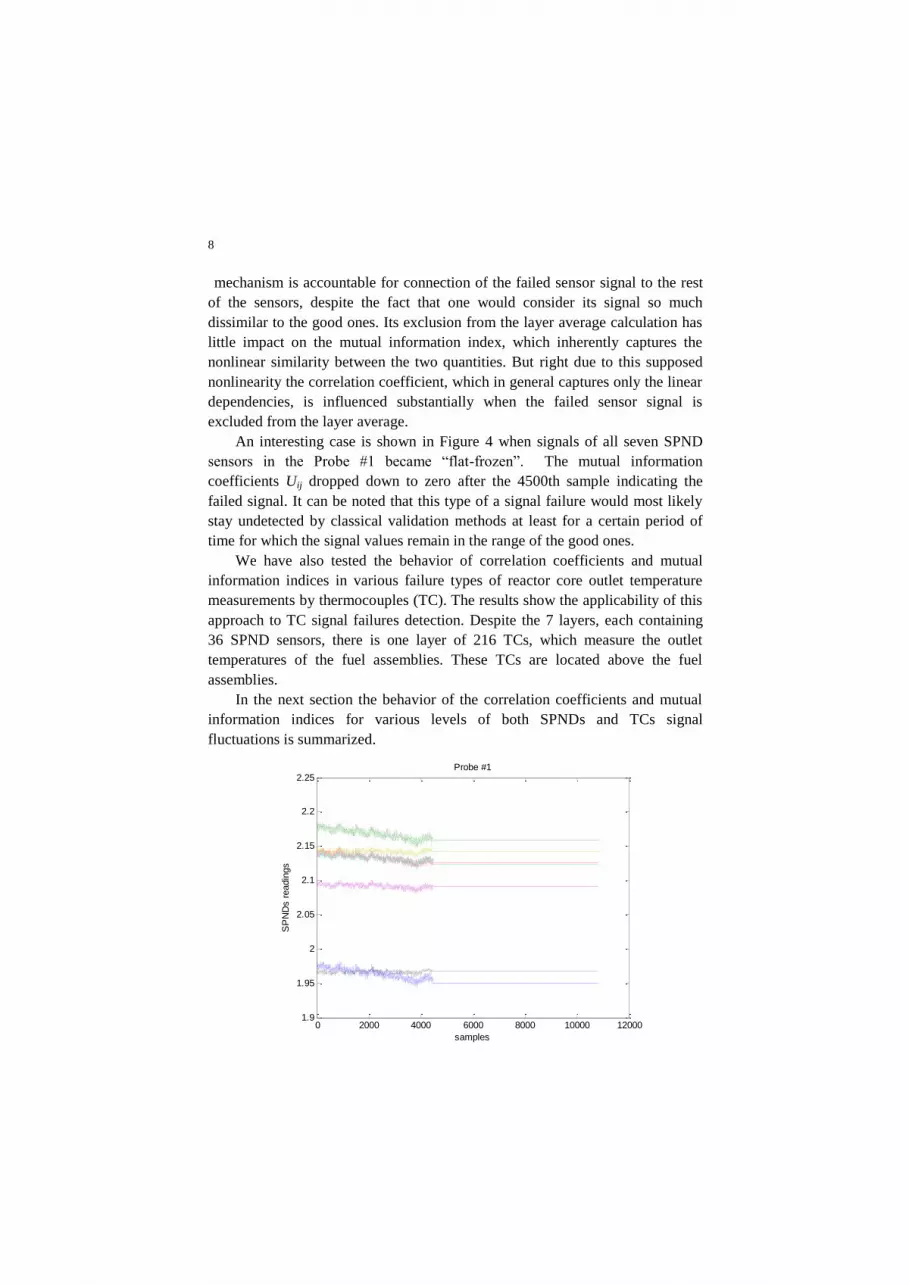
An interesting case is shown in Figure 4 when signals of all seven SPND

sensors in the Probe #1 became “flat-frozen”. The mutual information

coefficients Uij dropped down to zero after the 4500th sample indicating the

failed signal. It can be noted that this type of a signal failure would most likely

stay undetected by classical validation methods at least for a certain period of

time for which the signal values remain in the range of the good ones.

We have also tested the behavior of correlation coefficients and mutual

information indices in various failure types of reactor core outlet temperature

measurements by thermocouples (TC). The results show the applicability of this

approach to TC signal failures detection. Despite the 7 layers, each containing

36 SPND sensors, there is one layer of 216 TCs, which measure the outlet

temperatures of the fuel assemblies. These TCs are located above the fuel

assemblies.

In the next section the behavior of the correlation coefficients and mutual

information indices for various levels of both SPNDs and TCs signal

fluctuations is summarized.

0 2000 4000 6000 8000 10000 120001.9

1.95

2

2.05

2.1

2.15

2.2

2.25

samples

SP

ND

s r

eadin

gs

Probe #1

9

Figure 4. An example of the failed “flat-frozen” signals

2.4. Summary of correlation coefficients and mutual information indices

behavior

2.4.1. Self-powered neutron detectors

Correct signal

The dependence of the signal noise on the neutron flux fluctuations is obviously

quite straightforward and supposedly linear. All signals of correct sensors

fluctuate according to the fluctuating neutron flux. Their exclusion/inclusion

does not influence substantially the layer average and has only little impact on

correlation or mutual information coefficients. This mechanism can explain the

relatively high level of correlation coefficients while the mutual information

indices remain in the region of values of 0.3 to 0.4.

Bad signal with small fluctuations

Both correlation coefficients and mutual information indices are in the region of

low values. Because the signal’s low fluctuations do not influence the layer

average, the exclusion of the failed sensor from the average calculations is not

reflected in the correlation coefficients and mutual information indices.

Bad signal with big fluctuations

The vibrations of a failed sensor, having for example a cold junction between

the emitter and the leading wire, may affect its signal more severely. The

mechanical vibrations of the reactor core structures and sensors, including the

failed sensor itself, are in correlation with neutron flux fluctuations and

concurrently in certain and supposedly nonlinear link with the failed sensor

signal. Correlation coefficients and mutual information index are high in case

the failed sensor is included in the layer average calculations. After its exclusion

from layer average the correlation coefficients go down, while the mutual

information index remains high due to the supposed nonlinear link to the

neutron flux fluctuations.

Signal failure cause out of the reactor core

The behavior of the correlation coefficients and mutual information indices can,

at least in certain situations similar to the one encountered during the testing,

differentiate in-the-core from out-of-the-core source of failure when the failed

signal is caused by the electronic measuring circuits.

10

The strong fluctuations of the signal of the step-like shape influenced the layer

mean. It resulted in high Cij values. Excluding the signal from the layer mean

reflects in drop of Cij values, while the values of Uij indices remain practically

intact and in the range of the standard values.

2.4.2. Reactor core outlet thermocouples

Correct signal

The dependence of the signal noise on the coolant temperature fluctuations is

obviously quite straightforward and supposedly linear. All signals of correct

sensors fluctuate according to the fluctuating coolant temperatures. The

correlation coefficients are relatively high and the mutual information indices

remain in the average region of values of 0.15 to 0.35. The exclusion or

inclusion of the sensor from the layer average calculation does not influence

substantially the layer average and has only little impact on correlation or

mutual information coefficients.

Suspect signal having a raised level of noise

For suspect TC signals the correlation coefficients are set to the lower values

while the mutual information indices are increased above the average values.

Due to the high number of TCs in the reactor the exclusion or inclusion of the

suspect sensor from the layer average calculation does not influence

substantially the layer average and has only little impact on correlation or

mutual information coefficients.

Bad signal (noisy)

For noisy TC signals the correlation coefficients are set to the lower values

while the mutual information indices are increased high above the average

values. The exclusion or inclusion of the failed sensor from the layer average

calculation does not influence substantially the layer average and has only little

impact on correlation or mutual information coefficients.

Bad signal (very large fluctuations)

For TC signals degraded by the big fluctuations both correlation coefficients and

mutual information indices are high. While the correlation coefficient decreases

to low values after exclusion of the sensor from the layer average calculations,

the mutual information index remains high.

11

2.5. Signal features for failure detection

The consequent of various ways of behavior of correlation coefficients and

mutual information indices in different situations is that we cannot always rely

only on inspection of pure Cij and Uij coefficients. It may be recommended to

support the judgments by other methods making use of e.g. signal pattern

recognition techniques. The signal features, i.e. the signal patterns, can be

constructed e.g. based on the classical FFT power spectral density shape. The

other promising way of constructing the signal features can be based on signal's

wavelet transform coefficients [11]. They, we expect, will reflect the correct and

failed signal.

Figure 5. Haar wavelet coefficients based signal features

For illustration, let’s first calculate the differences between adjacent

elements of signal vector and then decompose this time series up to the level

five of details by Haar wavelets. The selected signal features might be the

maximum and minimum detail wavelet coefficients in each of five scales, see

Fig. 5. The solid lines connecting these features have no real meaning, they are

only to enhance the clarity. We can see that the failed and good signals’ features

form two distinct classes. The good ones are located in a very narrow strip while

1 2 3 4 5 6 7 8 9 10

-0.2

-0.15

-0.1

-0.05

0

0.05

0.1

0.15

0.2

minimum wavelet coefficients maximum wavelet coefficients

wavele

t coeff

icie

nt's v

alu

es

Signal features

+ for failed signals

O for correct signals

12

the failed ones are widely scattered. These patterns can easily be recognized

by properly trained artificial neural networks [12] or other classification

algorithms.

3. Diagnostics Based on Neuro-Fuzzy System Trained to Residuals

Direct validation of the SPND readings in [μA] encounters with a problem of

their dependence on ever changing fuel load patterns as well as the burn-up of

both fuel and SPNDs’ emitters. The training would normally have to be done on

simulated data prior to each fuel cycle. As mentioned above, the idea arose to

train PEANO to residuals instead, i.e. the differences between the core simulator

physics code results and their experimental counterpart values. It was supposed

that the system would be enough to train once.

The problem arises with the SPND readings, which are not directly

calculated by a core simulator. Instead, we define the residuals as follows:

residual = lin.powerSPND – lin.powerCORSIM (7)

Linear powerSPND of the fuel assembly at the location of the SPND is

proportional to the electric current measured from the detector and can be

calculated by the formula considering also the burn-up of both fuel and detector

emitter, temperature, power, vicinity of the fuel assembly, i.e. the fuel load

pattern, boron acid concentration, and uneven power distribution along the fuel

rods inside the fuel assembly. Linear powerCORSIM is calculated from 3D power

reconstruction by the reactor core physics code.

After the residual is validated by PEANO, the validated sensor signal will be

obtained as follows:

validated lin.powerSPND = validated residual + lin.powerCORSIM (8)

For the reactor core outlet temperature thermocouples the residuals are as

follows:

residual = fuel assembly powerTCs – fuel assembly powerCORSIM (9)

Fuel assembly powerTCs is calculated from the enthalpy difference related

to the fuel assemblies’ outlet and inlet temperatures while the fuel assembly

powerCORSIM is calculated from 2D power reconstruction by the reactor core

physics code.

It is expected that the residuals implicitly incorporate the reactor core

physics parameters such as the fuel load pattern and both fuel and SPND

emitters burn-up. If the linear powerSPND was measured/obtained exactly and at

13

the same time the linear powerCORSIM was also calculated exactly, then the

residual would equal zero. Apparently, this is hard to achieve and the individual

residuals differ more or less from zero as a consequent of inaccuracies of both

calculations and measurements. Nevertheless, as the fuel load pattern and burn-

up are implicitly incorporated in both types of linear power quantities

simultaneously, we may expect more systematic than random behavior of the

particular residuals. Besides, these residuals are supposed to depend on control

rod positions, power, and some other parameters. Analogically, we can expect

the same also for TC residuals.

3.1. Experiences from testing in successive fuel cycle-the batch training

PEANO was trained with data from one fuel cycle covering various operating

situations and then tested with data from the successive fuel cycle [13,14]. When

selecting the patterns of the previous fuel cycle into the training data files, we

focused our effort on including various operating situations, which can simply

be characterized by the reactor power. We gathered the data almost from the

whole campaign and tried to cover all situations occurred. We selected the great

number of patterns at the different reactor power levels. Although the reactor

power level during testing remained within the values involved in training, the

validation performance was not satisfactory. Due to the inaccuracies in both

calculations and measurements, the residuals have some systematic values

during the given fuel cycle. In contrast to the situation when training and testing

was performed with data from the same fuel cycle and validation performance

was excellent, this time the signal of some sensors were not modeled properly.

In the most cases, the biggest discrepancies between the measured and PEANO

predicted residuals of lin. power appeared when for these specific sensors the

values of residuals in the new campaign differed substantially from those in the

previous one, which PEANO was trained to. When we move to the next fuel

cycle, the reactor core has different parameters. The new fuel load pattern, the

fuel and SPNDs burn-up may have certain influence on the accuracy of

calculations resulting in the new pattern of the systematic deviations in the

residuals. For these sensors the residuals differ from those PEANO was trained

to and the validation performance deteriorates. Even though many other sensors

were modeled properly, the overall validation performance was unsatisfactory.

In the case of the reactor core outlet thermocouples the core simulator

calculates the integral power of the fuel assembly, which is more accurate than

the 3D power distribution. Moreover, the experimental values of the fuel

assemblies power derived from the difference of enthalpies related to the fuel

14

assemblies outlet and inlet temperatures are supposed to be more

straightforward and accurate than the calculation of the linear power of the fuel

assembly at the location of the SPND. Contrary to all expectations, the

validation performance for some TC sensors was also unsatisfactory.

Whatever the cause of the change of residuals in the other than the training

fuel cycle might be, the conclusion is that training to all possible operating

situation in one fuel cycle prior to its use in the successive ones is not a feasible

solution.

3.2. Incremental training and testing within the same fuel cycle

Despite the unsuccessful validation performance in the successive fuel cycles,

we did not want to abandon the idea of residuals due to their supposed property

to implicitly contain the reactor physics characteristics. Because the validation

performance was excellent within the same fuel cycle, the proposed solution was

to use the incremental training. Precondition for the successful performance was

that training was performed with data from the operation situations prior to the

current one, yet from the same cycle. In the beginning of the fuel cycle after the

reactor start-up the data were first acquired for about two weeks period of time

after which PEANO was trained and then used for signal validation. This

process continued as the fuel cycle proceeded, each time PEANO being

retrained with the new batch of data added to the previous one.

Regarding the SPND sensors, in the most cases the prediction of the

residual values was very good. Yet, there were the situations when the accuracy

deteriorated to five or even ten percent of linear power at the detector location. It

is to note that even we tried to tune the PEANO system by proper adjusting the

clustering and neural networks topology parameters during the training,

deliberately we did not strive for the best possible solution. We wanted to model

the operational staff/user behavior, who is not expected to act like this in the

real life implementation of such a diagnostic system and wants to have a

relatively simply functioning system. This may perhaps be responsible for the

deterioration of the signal predictions, which appeared from time to time.

Summarizing the above mentioned experience with SPND sensors

diagnostics brings up the conclusion that the usage of a system would be to a

certain extent cumbersome when constant attention by the repeated and not quite

easy retraining throughout the fuel cycle is to be given by the user while the

demanded accuracy may not be guaranteed. We therefore are not inclined to

recommend this approach for SPND sensors validation. This standpoint is

15

backed up by the fact that the SPND readings are of less importance to control

the reactor comparing to the TC readings.

3.2.1. Validation of core outlet thermocouples

In addition to the TC residuals the measurements of the reactor power, main

control rods positions, and overall flow rate through the reactor were added to

the model as inputs. For the sake of simplicity only 35 TCs from the 2nd

sector

were given to the input. Validating all 210 TCs at the same time would probably

be impossible as training of such huge neural networks would probably fail. It

means, if we wanted to validate all TCs, we would need to run in parallel 6

instances of the trained Peano system.

The number of middle hidden layer neurons was chosen close to the number

of principal components in data files. The topology of the neural networks was

kept unchanged during the whole process of retraining and testing. The so called

robust training was applied when different noise and faults were superimposed

on the input signals while the networks were trained to output the denoised

signals. This forces the neural networks to act as a noise filter. Similarly to the

SPNDs, the process started at the beginning of the cycle by about two weeks

data gathering which were then used to train the PEANO system. After this

period, within which PEANO could not be used for monitoring the signals, the

real monitoring phase could start. After another two to four weeks the acquired

data were added to the training set and the process was repeated.

A certain problem related to the incremental training can appear when a

new operational situation, not having been included during the previous training,

is encountered. It was the case at the end of the fuel cycle when the reactor

power was lowered to the levels very different from all the previous situations.

Figure 6 shows the typical shape of the prediction – the red line – when all the

monitored signals to be validated were correct. The system did not model the

signal (residual) behavior very correctly in the very end of the campaign; see the

last two sections of the predicted curve between the days 270 to 295. After the

data section between the days 270 to 280 was added to the previous training data

and the system was retrained, the prediction quality again improved, as it is

apparent in the very last section between the days 288 to 295.

16

Figure 6. The typical prediction of the correct TC residual

The other problem, which the incremental training in its substance bears, is

the influencing the prediction results by a drift in the input signals. If the drift is

small and not apparent on the first look, the corrupted signals are used in the

next training phase, which impairs the ability of the trained system to recognize

the deviations in the drifted signals. Five TCs were simulated to drift

simultaneously, each with the rate of 0.1°C/month immediately after the initial

two weeks training data gathering period. As supposed, after some time the

prediction performance degraded. Each time the system was retrained with the

previous section of data containing the drifted signals, the prediction was closer

to the drifted values, which was an unwanted property. For this reason the

testing was stopped soon.

To solve this problem, the retraining style was changed by replacing the

drifted signals by their predicted values. It resulted in much better elimination of

the drift; see Figure 7, which shows the typical performance. The blue line

represents the original not drifted signal (residual) and the green line is the

simulated drift. The prediction is shown by the red line. The initial part of the

prediction line in cyan represents the period of time of approx. one month before

we started to suspect the signals of drifting. This was how we tried to model the

real life use of the system. It roughly corresponds to the sensitivity of the

method, which was about 0.1°C deviation/fault in the measured temperatures.

Below this one cannot be sure whether it is the prediction error if just short

0 50 100 150 200 250 300-5

0

5

10

15

20x 10

4 TC-55

fuel

ass

em

bly

po

we

r re

sid

ua

l [w

]

[days]

17

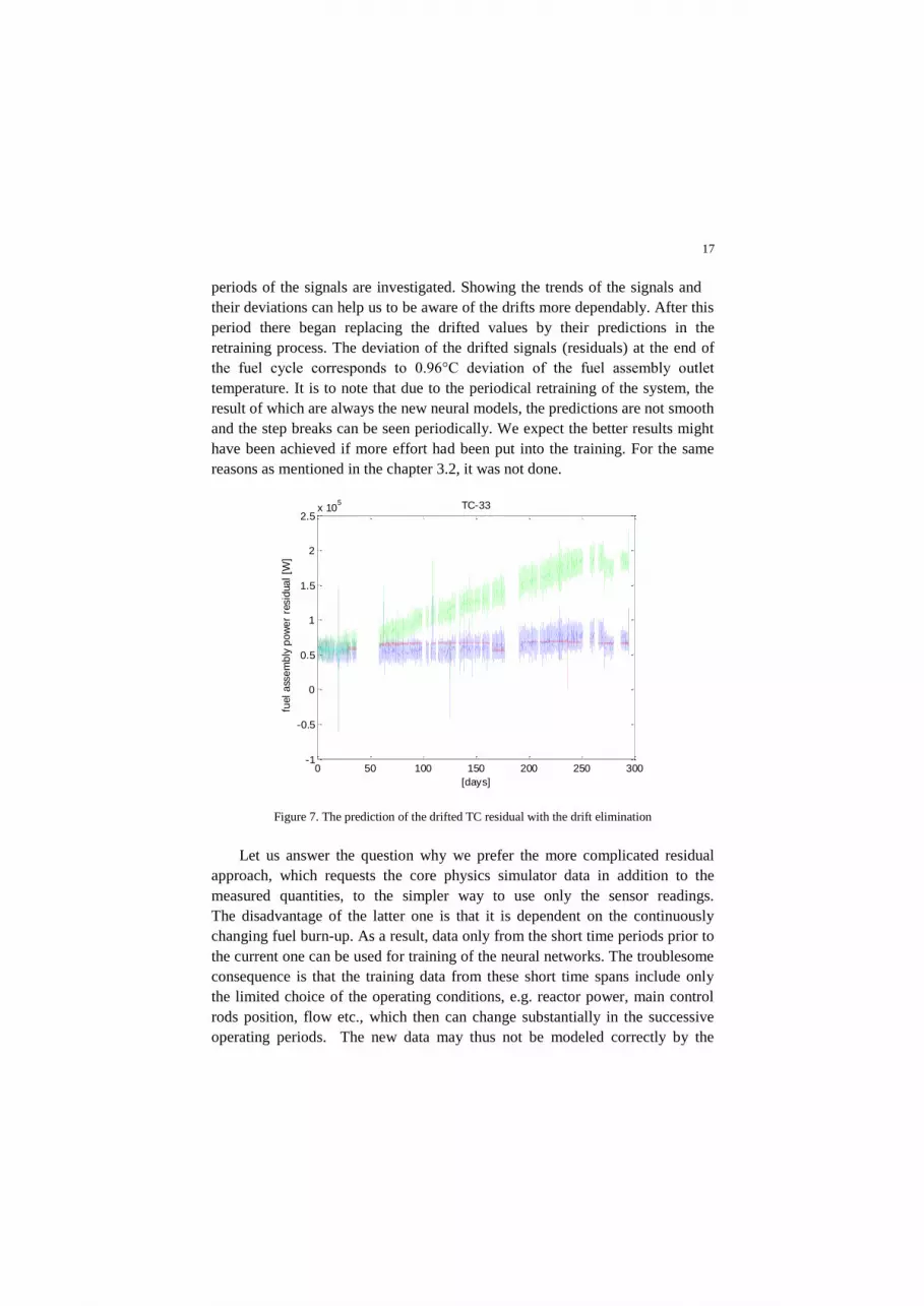
periods of the signals are investigated. Showing the trends of the signals and

their deviations can help us to be aware of the drifts more dependably. After this

period there began replacing the drifted values by their predictions in the

retraining process. The deviation of the drifted signals (residuals) at the end of

the fuel cycle corresponds to 0.96°C deviation of the fuel assembly outlet

temperature. It is to note that due to the periodical retraining of the system, the

result of which are always the new neural models, the predictions are not smooth

and the step breaks can be seen periodically. We expect the better results might

have been achieved if more effort had been put into the training. For the same

reasons as mentioned in the chapter 3.2, it was not done.

Figure 7. The prediction of the drifted TC residual with the drift elimination

Let us answer the question why we prefer the more complicated residual

approach, which requests the core physics simulator data in addition to the

measured quantities, to the simpler way to use only the sensor readings.

The disadvantage of the latter one is that it is dependent on the continuously

changing fuel burn-up. As a result, data only from the short time periods prior to

the current one can be used for training of the neural networks. The troublesome

consequence is that the training data from these short time spans include only

the limited choice of the operating conditions, e.g. reactor power, main control

rods position, flow etc., which then can change substantially in the successive

operating periods. The new data may thus not be modeled correctly by the

0 50 100 150 200 250 300-1

-0.5

0

0.5

1

1.5

2

2.5x 10

5 TC-33

[days]

fuel

ass

em

bly

po

we

r re

sid

ua

l [W

]

18

neural models created in the previous period of time. On the contrary, the

residual approach comprises the burn-up and other reactor physics

characteristics. The various operating conditions are involved incrementally in

the data coming from the previous time periods. The incremental training is

supposed to enable the use of the trained system for longer periods. The other

reason for using residuals is that the system can be more sensitive and reveal

even very small deviations in the sensor readings in spite of modeling the

signals’ full range. On the other hand, the negative consequence of using

residuals is that more factors are to be used in the procedure of deriving the

power residuals from measured input and output temperatures using functions

for calculating equivalent enthalpies and vice versa back to the validated

temperatures, each contributing to the overall uncertainty of the result.

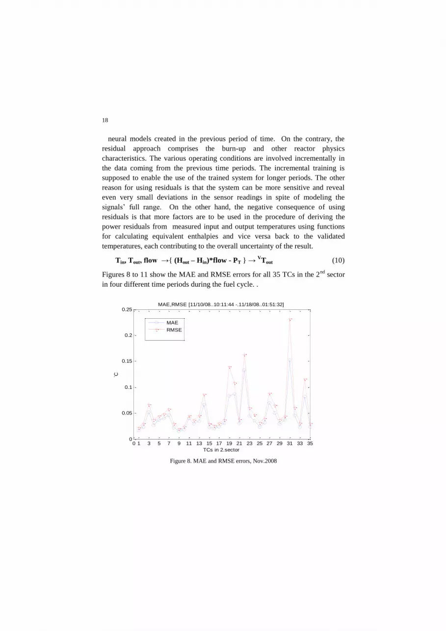
Tin, Tout, flow →{ (Hout – Hin)*flow - PT } → VTout (10)

Figures 8 to 11 show the MAE and RMSE errors for all 35 TCs in the 2nd

sector

in four different time periods during the fuel cycle. .

Figure 8. MAE and RMSE errors, Nov.2008

0 1 3 5 7 9 11 13 15 17 19 21 23 25 27 29 31 33 350

0.05

0.1

0.15

0.2

0.25MAE,RMSE [11/10/08..10:11:44 -.11/18/08..01:51:32]

TCs in 2.sector

`C

MAE

RMSE

19

Figure 9. MAE and RMSE errors, March 2009

Figure 10. MAE and RMSE errors, June 2009

0 1 3 5 7 9 11 13 15 17 19 21 23 25 27 29 31 33 350

0.05

0.1

0.15

0.2

0.25MAE,RMSE [02/26/09..01:01:02 -.03/21/09..04:12:03]

TCs in 2.sector

`C

MAE

RMSE

0 1 3 5 7 9 11 13 15 17 19 21 23 25 27 29 31 33 350

0.05

0.1

0.15

0.2

0.25MAE,RMSE [05/03/09..20:51:22 -.06/13/09..12:10:15]

TCs in 2.sector

`C

MAE

RMSE

20

Figure 11, MAE, RMSE, July,2009

It is to notice that the mean absolute error for TC#29 in the 2nd

symmetry

sector increased approximately 3 times in July. Figure 12 shows the prediction

of validated outlet temperatures - the red line - during the fuel cycle. It is

apparent that only after the day of approximately 200 a deviation appeared. Why

the predictions before this time were in quite good congruence with the drifted

values can be explained by the very low drift of only 0.025 °C/month, see

Figure 13 showing the trends of all TC#29 symmetry orbits. Closer investigation

shows that in this time the deviation from the rest of TCs in the symmetry orbit

increased slightly, which reflected in the prediction divergence. The other very

important reason is that unnoticed drifted values infiltrated the training data. It

impaired the ability of trained system to recognize the deviating drifted signal.

Each time the system was retrained with the previous section of data containing

the degraded signal, the prediction was close to the drifted values. It is to say

that the estimated sensitivity of the method is about 0.1°C deviation/fault in the

measured temperatures. It was also the limit for our investigation how the

method was capable to cope with the drifts. Below this one cannot be sure

whether it is the prediction error if just short periods of the signals are

investigated. Showing the trends of the signals and their deviations can help us

to be aware of the drifts more dependably, as confirmed by Figures 12 and 13.

0 1 3 5 7 9 11 13 15 17 19 21 23 25 27 29 31 33 350

0.05

0.1

0.15

0.2

0.25MAE,RMSE [07/05/09..17:02:04 -.07/30/09..09:23:11]

TCs in 2.sector

`C

MAE

RMSE

21

Figure 12, Prediction for TC 29

Figure 13, All TCs 29 on the symmetry orbit

50 100 150 200 250

302.5

303

303.5

304

304.5

305

305.5

306

306.5

307

TC 29 in symmetry sector #2

[ days ]

T [

' C

]

0.5 1 1.5 2 2.5

x 105

303

304

305

306

307

308

T [

'C

]

symmetrical TCs 29

samples

drift ~ 0.025 `C/month

22

Figure 14, Prediction performance in transient

Figure 15, Prediction performance in transient

200 400 600 800 1000 1200 1400

280

285

290

295

300

305

TC 11; transient 55% nominal power

samples

T [

'C ]

measured values

prediction

200 400 600 800 1000 1200 1400

285

290

295

300

305

samples

T [

'C

]

TC 14; transient 55% nominal power

measured values

prediction

360 370 380 390 400 410 420 430 440 450 460

282.5

283

283.5

284

284.5

285

360 370 380 390 400 410 420 430 440 450 460

280

280.5

281

281.5

282

23

Figures 14 and 15 show the prediction performance during a transient of

55 %. reactor power. Mostly the prediction error was below 0.1 °C, rarely up to

0.4 °C as can be seen in Figure 15. It is well known that the empirical models

like the artificial neural networks perform well in the situations having been

included in the training data. The reactor was mostly operated at the nominal

power level, while there were only few situations of lower power. Therefore, the

close to nominal power data were vastly prevailing in the training files. The very

important issue for a user is to know that the system has not been trained

properly to recognize the current situation and the system’s statements/results of

validation can thus be less dependable. The Peano system incorporates this

feature by evaluating the running degree of reliability.

4. Conclusions

In this work we outline two approaches to in-core sensor validation and present

our first experience. The first one is based on correlation of signals, both in

linear and nonlinear regions, and makes use of the signal fluctuations, which

have their source in perturbations present in the reactor core. It is assumed that

the decreasing similarity of signals is the manifestation of a sensor failure. The

results show the applicability of linear correlation coefficients and mutual

information based criteria to the SPNDs and TCs signal failures detection.

Though this method cannot calculate the expected values of the signals and can

serve “only” for diagnostic purposes, yet it might have an asset to I&C people. It

is also to mention that this method is easy to implement. Authors of ref. [6] even

describe their experience with the ability of the correlation approach to reveal

future sensor failing.

On the other hand, the consequence of specific behavior of both correlation

coefficients and mutual information indices in different situations is that we

should not rely only on their examination. We may want to support our

judgments by other methods making use of e.g. signal pattern recognition

techniques and/or fuzzy logic based inferential algorithms. For example, the

signal features can be constructed based on the wavelet transform coefficients

and/or on the Fast Fourier Transform (FFT) power spectral density shape. They,

we expect, will reflect the correct and failed signal. These patterns could then

easily be recognized by the properly trained artificial neural networks or other

pattern recognition algorithms. The labeling of the failed sensor by statistical

hypothesis testing could be in disputable cases supported by fuzzy logic

inferential algorithms based judgments.

24

The second approach, we were examining, is based on the neuro-fuzzy

modeling of residuals instead of the raw measured values. Residuals are the

differences between the core simulator physics code results and their

experimental counterpart values. We found out that the original idea to train the

neuro-fuzzy system to residuals acquired during one fuel cycle and then using

the trained system in the following ones failed. The remedy to this can be the

incremental training, the process of which is as follows: In the beginning of the

fuel cycle after the reactor start-up the data were first acquired for about two

weeks period of time after which the system was trained and then used for signal

validation. This process continued as the fuel cycle proceeded, each time the

system being retrained with the new batch of data added to the previous one.

The price the user would pay for such a system would be its relatively

cumbersome usage when constant attention by the repeated and not quite easy

retraining throughout the fuel cycle is to be given by the user. In addition to this,

the demanded validation accuracy for SPNDs may not be guaranteed, which is

the reason why we are not inclined to recommend this approach for SPND

sensors validation with their lesser significance in reactor control.

In contrast to the SPNDs, the residual approach to validation of core outlet

TC signals is able to recognize the multiple TC signal failures in the very early

stages of their occurrence. The achieved accuracy of the signal prediction was

mostly better than 0.1°C at the full range of 300°C. It is to mention that the

incremental training, by its very nature, cannot function from the very beginning

of the fuel cycle, as the training data has to be acquired first after the reactor

start-up. The good thing is that within this relatively short time period the

reactor undergoes more power maneuvering and operating conditions, which

makes input data enough diverse for successful training. The unwanted

consequence of the need for initial training at the fuel cycle beginning is that the

systematic errors in TC readings, which may appear right after the reactor start-

up and will be contained in the training data, will not be discovered. The user

will have to rely on an independent approach, e.g. based on the symmetry of the

reactor core.

Our investigation has shown that the neuro-fuzzy residual approach is able

to recognize multiple simultaneous failures with a very good accuracy but at a

cost of a cumbersome use due to the need of a periodical retraining and

replacement of the failed readings by predictions. The real implementation of

this technique would require the development of a new more user friendly

system, which would automatically ensure most of the manual interventions.

Nevertheless, it can be concluded that the reliable signal diagnostics and/or

25

validation can be achieved only by a combination of various techniques able

to capture a variety of failures.

Acknowledgments

This paper is the result of implementation of the project: Increase of Power

Safety of the Slovak Republic (ITMS: 26220220077) supported by the Research

& Development Operational Program funded by the ERDF.

References

1. P.F.Fantoni, S. Figedy,B. Papin, A neuro-fuzzy model applied to full range signal validation of PWR nuclear power plant data. Second OECD Specialist Meeting on Operator Aids for Severe Accident Management (SAMOA-2), Lion, (1997)

2. S.Figedy, Real-Time Process Signal Validation based on Neuro-Fuzzy and

possibilistic Approach, ICANN98, Skovde, Sweden,Sept.2-4, (1998)

3. P. Fantoni, M. Hoffmann, R. Shankar, E. Davis, “On-Line Monitoring of

Instrument Channel Performance in Nuclear Power Plant Using PEANO”,

Progress in Nuclear Energy, Vol. 43, No. 1-4, (2003)

4. M. Hoffmann, “On-line Calibration Monitoring with PEANO”,

NPIC&HMIT 2004, Columbus, Ohio, September (2004)

5. S.Figedy, Outline of In-Core Sensor Validation Based on Correlation and

Mutual Information Analysis, NPIC&HMIT2006, Albuquerque, New

Mexico, Nov.12-16,(2006)

6. F.Adorjan and T.Morita, A Correlation-Based Signal Validation Method for

Fixed In-Core Detectors, Nuclear Technology, 118,264 (1997).

7. R.M.Gray, Entropy and Information Theory, Springer-Verlag (1990)

8. C.E.Shannon, A Mathematical Theory of Communication,

http://cm.bell-labs.com/ cm/ms/what/shannonday/paper.html

9. I.J.Taneja, Generalized Information Measures and Their Applications,

http://www.mtm.ufsc.br/~taneja/book/book.html

10. Numerical Recipes in Fortran 77, http://www.nr.com

11. G.Strang and T.Nguyen, Wavelets and Filter Banks, Wellesley-Cambridge

Press (1996)

12. L.H.Tsoukalas and R.H.Uhrig, Fuzzy and Neural Approaches in

Engineering, John Wiley &Sons (1999)

13. S.Figedy, Outline of New Approaches to In-Core Sensor Validation Based

on Modern Signal Processing and Neuro-Fuzzy Techniques, NPIC&HMIT

2009, Knoxville, Tennessee, Apr.5-9,(2009)

26

14. S.Figedy, Experiences with Residual Approach to Validation of In-Core

Sensors by PEANO Neuro-Fuzzy System, NPIC&HMIT 2010, Las Vegas,

Nevada, Nov.7-11,(2010)