galaxy and mass assembly (gama): survey diagnostics and core data release

arX

iv:1

009.

0614

v1 [

astr

o-ph

.CO

] 3

Sep

201

0Mon. Not. R. Astron. Soc. 000, 1–27 (2010) Printed 6 September 2010 (MN LATEX style file v2.2)

Galaxy and Mass Assembly (GAMA): survey diagnosticsand core data release

S.P.Driver1⋆, D.T.Hill1, L.S.Kelvin1, A.S.G.Robotham1, J.Liske2, P.Norberg3, I.K.Baldry4,

S.P.Bamford5, A.M.Hopkins6, J.Loveday7, J.A.Peacock3, E.Andrae8, J.Bland-Hawthorn9,

S.Brough6, M.J.I.Brown10, E.Cameron11, J.H.Y.Ching9, M.Colless6, C.J.Conselice5,

S.M.Croom9, N.J.G.Cross3, R.De Propris12, S.Dye13 M.J.Drinkwater14, S.Ellis9,

Alister W.Graham15, M.W.Grootes15, M.Gunawardhana8, D.H.Jones6, E.van Kampen2,

C.Maraston12, R.C.Nichol16, H.R.Parkinson3, S.Phillipps17, K.Pimbblet10, C.C.Popescu18,

M.Prescott4, I.G.Roseboom7, E.M.Sadler9, A.E.Sansom18, R.G.Sharp6, D.J.B.Smith5,

E.Taylor8,20, D.Thomas16, R.J.Tuffs8, D.Wijesinghe9, L.Dunne5, C.S.Frenk22, M.J.Jarvis23,

B.F.Madore24, M.J.Meyer25, M.Seibert24, L.Staveley-Smith25, W.J.Sutherland26, S.J.Warren27

1 School of Physics & Astronomy, University of St Andrews, North Haugh, St Andrews, KY16 9SS, UK; SUPA2 European Southern Observatory, Karl-Schwarzschild-Str. 2, 85748, Garching, Germany3 Institute for Astronomy, University of Edinburgh, Royal Observatory, Blackford Hill, Edinburgh, EH9 3HJ, UK4 Astrophysics Research Institute, Liverpool John Moores University, Twelve Quays House, Egerton Wharf, Birkenhead, CH4 1LD, UK5 Centre for Astronomy and Particle Theory, University of Nottingham, University Park, Nottingham, NG7 2RD, UK6 Australian Astronomical Observatory, PO Box 296, Epping, NSW 1710, Australia7 Astronomy Centre, University of Sussex, Falmer, Brighton, BN1 9QH, UK8 Max-Plank Institute for Nuclear Physics (MPIK), Saupfercheckweg 1, 69117 Heidelberg, Germany9 Sydney Institute for Astronomy, School of Physics, University of Sydney, NSW 2006, Australia10 School of Physics, Monash University, Clayton, Victoria 3800, Australia11 Department of Physics, Swiss Federal Institute of Technology (ETH-Zurich), 8093 Zurich, Switzerland12 Cerro Tololo Inter-American Observatory, La Serena, Chile13 School of Physics and Astronomy, Cardiff University, Queens Buildings, The Parade, Cardiff, CF24 3AA, UK14 Department of Physics, University of Queensland, Brisbane, Queensland 4072, Australia15 Centre for Astrophysics and Supercomputing, Swinburne University of Technology, Hawthorn, Victoria 3122, Australia16 Institute of Cosmology and Gravitation (ICG), University of Portsmouth, Dennis Sciama Building Road, Portsmouth, PO1 3FX, UK17 Astrophysics Group, H.H. Wills Physics Laboratory, University of Bristol, Tyndall Avenue, Bristol BS8 1TL, UK18 Jeremiah Horrocks Institute, University of Central Lancashire, Preston, PR1 2HE, UK19 Instituto Astronomico e Geoffisico, University of San Paulo, Brazil20 School of Physics, University of Melbourne, Victoria 3010, Australia21 Institute for Computational Cosmology, Department of Physics, University of Durham South Road, Durham, DH1 3LE, UK22 Centre for Astrophysics, Science & Technology Research Institute, University of Hertfordshire, Hatfield, AL10 9AB, UK23 Observatories of the Carnegie Institute of Washington, 813 Santa Barbara Street, Pasadena, CA91101, USA24 International Centre for Radio Astronomy Research, The University of Western Australia, 35 Stirling Hwy, Crawley, WA 6009, Australia25 Astronomy Unit, Queen Mary University London, Mile End Road, London, E1 4NS, UK26 Astrophysics Group, Imperial College London, Blackett Laboratory, Prince Consort Road, London, SW7 2AZ, UK

6 September 2010

ABSTRACTThe Galaxy And Mass Assembly (GAMA) survey has been operating since February2008 on the 3.9-m Anglo-Australian Telescope using the AAOmega fibre-fed spec-trograph facility to acquire spectra with a resolution of R ≈ 1300 for 120 862 SDSSselected galaxies. The target catalogue constitutes three contiguous equatorial regionscentred at 9h (G09), 12h (G12) and 14.5h (G15) each of 12× 4 deg2 to limiting fluxesof rpet < 19.4, rpet < 19.8, and rpet < 19.4 mag respectively (and additional limitsat other wavelengths). Spectra and reliable redshifts have been acquired for over 98per cent of the galaxies within these limits. Here we present the survey footprint,progression, data reduction, redshifting, re-redshifting, an assessment of data qualityafter 3 years, additional image analysis products (including ugrizY JHK photome-try, Sersic profiles and photometric redshifts), observing mask, and construction ofour core survey catalogue (GamaCore). From this we create three science ready cata-logues: GamaCoreDR1 for public release, which includes data acquired during year 1 ofoperations within specified magnitude limits (February 2008 to April 2008); GamaCore-MainSurvey containing all data above our survey limits for use by the GAMA teamand collaborators; and GamaCoreAtlasSv containing year 1, 2 and 3 data matchedto Herschel-ATLAS Science Demonstration data. These catalogues along with theassociated spectra, stamps, and profiles, can be accessed via the GAMA website:http://www.gama-survey.org/

c© 2010 RAS

http://arxiv.org/abs/1009.0614v1

http://www.gama-survey.org/

2 Driver et al. — DRAFT v3.1

1 INTRODUCTION

Large scale surveys are now a familiar part of the astronomylandscape and assist in facilitating a wide range of scienceprogrammes. Three of the most notable wide-area surveysin recent times, with a focus on galactic and galaxy evolu-tion, are the 2 Micron All Sky Survey (2MASS; Skrutskie etal. 2006), the 2 degree Field Galaxy Redshift Survey (2dF-GRS; Colless et al. 2001; 2003), and the Sloan Digital SkySurvey (SDSS; York et al. 2000). These surveys have eachbeen responsible for a wide range of science advances at-tested by their publication and citation records (Trimble &Ceja 2010), ranging from: the identification of new stellartypes (e.g., Kirkpatrick et al., 1999); tidal streams in theGalactic Halo (e.g., Belokurov et al. 2006); new populationsof dwarf galaxies (e.g., Willman et al. 2005); galaxy popu-lation statistics (e.g., Bell et al. 2003; Baldry et al. 2006);the recent cosmic star-formation history (e.g., Heavens etal. 2004); group catalogues (e.g., Eke et al. 2004); mergerrates (e.g., Bell et al., 2006); quantification of large scalestructure (e.g., Percival et al. 2001); galaxy clustering (e.g.,Norberg et al. 2001); and, in conjunction with CMB andSNIa searches, convergence towards the basic cosmologicalmodel now adopted as standard (e.g., Spergel et al. 2003;Cole et al. 2005). In addition to these mega-surveys therehave been a series of smaller, more specialised, local sur-veys including the Millennium Galaxy Catalogue (MGC;Driver et al., 2005), the 6dF Galaxy Survey (6dFGS; Joneset al. 2004, 2009), the HI Parkes All Sky Survey (HIPASS;Meyer et al. 2004), and the Galaxy Evolution Explorer(GALEX; Martin et al. 2005) mission, which are each open-ing up new avenues of extra-galactic exploration (i.e., struc-tural properties, the near-IR domain, the 21cm domain, andthe UV domain respectively). Together these surveys pro-vide an inhomogeneous nearby reference point for the verynarrow high-z pencil beam surveys underway (i.e., DEEP2,VVDS, COSMOS, GEMS etc.), and from which compara-tive studies can be made to quantify the process of galaxyevolution (e.g., Cameron & Driver 2007).

The Galaxy And Mass Assembly Survey (GAMA) hasbeen established with two main sets of aims, which are sur-veyed in Driver et al. (2009). The first is to use the galaxydistribution to conduct a series of tests of the Cold DarkMatter (CDM) paradigm, and the second is to carry out de-tailed studies of the internal structure and evolution of thegalaxies themselves.

The CDM model is now the standard means by whichdata relevant to galaxy formation and evolution are inter-preted, and it has met with great success on 10–100 Mpcscales. The next challenge in validating this standard modelis to move beyond small linear fluctuations, into the regimedominated by dark-matter haloes. The fragmentation of thedark matter into these roughly spherical virialized objectsis robustly predicted both numerically and analytically overseven orders of magnitude in halo mass (e.g., Springel et al.2005). Massive haloes are readily identified as rich clustersof galaxies, but it remains a challenge to probe further downthe mass function. For this purpose, one needs to identifylow-mass groups of galaxies, requiring a survey that probesfar down the galaxy luminosity function over a large rep-resentative volume. But having found low-mass haloes, thegalaxy population within each halo depends critically on the

interaction between the baryon processes (i.e., star forma-tion rate and feedback efficiency) and the total halo mass.In fact the ratio of stellar mass to halo mass is predicted(Bower et al. 2006; De Lucia et al. 2006) to be stronglydependent on halo mass, exhibiting a characteristic dip atLocal Group masses. The need for feedback mechanisms tosuppress star formation in both low mass haloes (via su-pernovae) and high mass haloes (via AGN) is now part ofstandard prescriptions in modeling galaxy formation. WithGAMA we can connect these theoretical ingredients directlywith observational measurements.

However, the astrophysics of galaxy bias is not the onlypoorly understood area in the CDM model. Existing suc-cesses have been achieved at the price of introducing DarkEnergy as the majority constituent of the Universe, and akey task for cosmology is to discriminate between variousexplanations for this phenomenon: a cosmological constant,time varying scalar field, or a deficiency in our gravity model.These aspects can be probed by GAMA in two distinctways: either the form or evolution of the halo mass func-tion may diverge from standard predictions of gravitationalcollapse in the highly nonlinear regime, or information onnon-standard models may be obtained from velocity fields on10-Mpc scales. The latter induce redshift-space anisotropiesin the clustering pattern, which measure the growth rateof cosmic structure (e.g., Guzzo et al. 2008). Thus GAMAhas the potential to illuminate both the astrophysical andfundamental aspects of the CDM model.

Moving beyond the large-scale distribution, GAMA’smain long-term legacy will be to create a uniform galaxydatabase, which builds on earlier local surveys in a compre-hensive manner to fainter flux levels, higher redshift, higherspatial resolution, and spanning UV to radio wavelengths.The need for a combined homogeneous, multiwavelength,and spatially resolved study can be highlighted by three top-ical issues:

1. Galaxy Structure. Galaxies are typically comprised ofbulge and/or disc components that exhibit distinct prop-erties (dynamics, ages, metallicities, profiles, dust and gascontent), indicating potentially distinct evolutionary paths(e.g., cold smooth and hot lumpy accretion; cf. Driver etal. 2006 or Cook et al. 2010). This is corroborated by the ex-istence of the many SMBH-bulge relations (see, for example,Novak, Faber & Dekel 2006), which firmly couples spheroid-only evolution with AGN history (Hopkins et al. 2006). Acomprehensive insight into galaxy formation and evolutiontherefore demands consideration of the structural compo-nents requiring high spatial resolution imaging on ∼ 1 kpcscales or better (e.g., Allen et al. 2006; Gadotti 2009).

2. Dust attenuation. A recent spate of papers (Shao etal. 2007; Choi et al. 2007; Driver et al. 2007, 2008; Masterset al. 2010) have highlighted the severe impact of dust atten-uation on the measurement of basic galaxy properties (e.g.,fluxes and sizes). In particular, dust attenuation is highlydependent on wavelength, inclination, and galaxy type withthe possibility of some further dependence on environment.Constructing detailed models for the attenuation of stellarlight by dust in galaxies and subsequent re-emission (e.g.,Popescu et al. 2000), is intractable without extensive wave-length coverage extending from the UV through to the far-IR. To survey the dust content for a significant sample ofgalaxies therefore demands a multi-wavelength dataset ex-

c© 2010 RAS, MNRAS 000, 1–27

GAMA — DRAFT v3.1 3

tending over a sufficiently large volume to span all environ-ments and galaxy types. The GAMA regions are or will besurveyed by the broader GALEX Medium Imaging Surveyand Herschel-ATLAS (Eales et al. 2010) programmes, pro-viding UV to FIR coverage for a significant fraction of oursurvey area.

3. The HI content. As star-formation is ultimately drivenby a galaxy’s HI content any model of galaxy formation andevolution must be consistent with the observed HI properties(see for example discussion in Hopkins, McClure-Griffiths &Gaensler 2008). Until recently probing HI beyond very lowredshifts has been laborious if not impossible due to ground-based interference and/or sensitivity limitations (see for ex-ample Lah et al. 2009). The new generation of radio arraysand receivers are using radio-frequency interference mitiga-tion methods coupled with new technology receivers to openup the HI Universe at all redshifts (i.e., ASKAP, MeerKAT,LOFAR, and ultimately the SKA). This will enable coherentradio surveys that are well matched in terms of sensitivityand resolution to optical/near-IR data. Initial design studyinvestment has been made in the DINGO project, whichaims to conduct deep HI observations within a significantfraction of the GAMA regions using ASKAP (Johnston etal. 2007).

The GAMA survey will eventually provide a wide-area highly complete spectroscopic survey of over400k galaxies with sub-arcsecond optical/near-IR imag-ing (SDSS/UKIDSS/VST/VISTA). Complementary multi-wavelength photometry from the UV (GALEX), mid-IR (WISE) and far-IR (Herschel) and radio wavelengths(ASKAP, GMRT) is being obtained by a number of inde-pendent public and private survey programmes. These ad-ditional data will ultimately be ingested into the GAMAdatabase as they becomes available to the GAMA team. Atthe heart of the survey is the 3.9-m Anglo Australian Tele-scope (AAT), which is being used to provide the vital dis-tance information for all galaxies above well specified flux,size and isophotal detection limits. In addition the spec-tra from AAOmega for many of the sample will be of suffi-ciently high signal-to-noise and spectral resolution (≈ 3 —6 A) to allow for the extraction of line diagnostic informa-tion leading to constraints on star-formation rates, velocitydispersions and other formation/evolutionary markers. Thearea and depth of GAMA compared to other notable surveysis detailed in Baldry et al. (2010; their Fig. 1). In generalGAMA lies in the parameter space between that occupiedby the very wide shallow surveys and the deep pencil beamsurveys and is optimised to study structure on ∼ 10 h−1 Mpcto 1h−1 kpc scales, as well as sample the galaxy populationfrom FUV to radio wavelengths.

This paper describes the first three years of the GAMAAAOmega spectroscopic campaign, which has resulted in112k new redshifts (in addition to the 19k already knownin these regions). In section 2 we describe the spectroscopicprogress, data reduction, redshifting, re-redshifting, an as-sessment of the redshift accuracy and blunder rate, and anupdate to our initial visual classifications. In section 3 wedescribe additional image analysis resulting in ugrizY JHKmatched aperture photometry, Sersic profiles, and photo-metric redshifts. In section 4 we describe the combination ofthe data presented in section 2 and 3 to form our core cat-alogue and investigate the completeness versus magnitude,

colour, surface brightness, concentration, and close pairs. Insection 5 we present the survey masks required for spatialclustering studies and in section 6 present our publicly avail-able science ready catalogue. These catalogues along withan MYSQL tool and other data inspection tools are nowavailable at: http://www.gama-survey.org/ and we expectfuture releases of redshifts and other data products to occuron an approximately annual cycle.

Please note all magnitudes used in this paper, unlessotherwise specified, are r-band Petrosian (rpet) from SDSSDR6, which have been extinction corrected and placed ontothe true AB scale following the prescription described by theSDSS DR6 release (Adelman-McCarthy et al. 2008).

2 THE GAMA AAT SPECTROSCOPICSURVEY

2.1 GAMA field selection, input catalogue andtiling algorithm

The initial GAMA survey consists of three equatorial re-gions, each of 12 × 4 deg2 (see Table 1 and Fig. 1). Thedecision for this configuration was driven by three consider-ations: suitability for large-scale structure studies demand-ing contiguous regions of ∼ 50 deg2 to fully sample ∼ 100co-moving h−1 Mpc structures at z ≈ 0.2; observability de-manding a 5 hr Right Ascension baseline to fill a night’sworth of observations over several lunations; and overlapwith existing and planned surveys, in particular the SDSS(York et al. 2000), UKIDSS LAS (Lawrence et al. 2007),VST KIDS, VISTA VIKING, H-ATLAS (Eales et al. 2010),and ASKAP DINGO. Fig. 1 shows the overlap of some ofthese surveys. Note the H-ATLAS SGP survey region haschanged since Fig. 5 of Driver et al. (2009) due to additionalspace-craft limitations introduced in-flight. The depth andarea of the GAMAAAT spectroscopic survey were optimisedfollowing detailed simulations of the GAMA primary sciencegoal of measuring the Halo Mass Function. This resulted inan initial survey area of 144 deg2 to a depth of rpet < 19.4mag in the 9h and 15h regions and an increased depth ofrpet < 19.8 mag in the 12h region (see Table 1). In additionfor year 2 and 3 observations additional K and z-band selec-tion was introduced such that the final main galaxy sample(Main Survey) can be defined (see Baldry et al., 2010) asfollows:

G09: rpet < 19.4 OR (KKron < 17.6 AND rmodel < 20.5) OR

(zmodel < 18.2 AND rmodel < 20.5) mag





with all magnitudes expressed in AB. For the remainderof this paper we mainly focus, for clarity, on the r-bandselected data and note that equivalent diagnostic plots tothose shown later in this paper can easily be created for thez and K selections.

c© 2010 RAS, MNRAS 000, 1–27



Table 1. Coordinates of the three GAMA equatorial fields.

Field RA(J2000 deg.) Dec(J2000 deg.) Area (deg2) Depth (mag)

G09 129.0...141.0 +3.0...− 1.0 12 × 4 rpet < 19.4G12 174.0...186.0 +2.0...− 2.0 12 × 4 rpet < 19.8G15 211.5...223.5 +2.0...− 2.0 12 × 4 rpet < 19.4

Figure 1. GAMA Phase I (black squares) in relation to other recent and planned surveys (see key). For a zoom in to the GAMA regionsshowing SDSS, UKIDSS and GALEX overlap please see Fig. 1 of the companion paper describing the photometry by Hill et al., (2010a).Also overlaid as grey dots are all known redshifts at z < 0.1 taken from NASA ExtraGalactic Database.

2.2 Survey preparation

The input catalogue for the GAMA spectroscopic surveywas constructed from SDSS DR6 (Adelman-McCarthy etal. 2008) and our own reanalysis of UKIDSS LAS DR4(Lawrence et al. 2007) to assist in star-galaxy separation; seeHill et al. (2010a) for details. The preparation of the inputcatalogue, including extensive visual checks and the revisedstar-galaxy separation algorithm, is described and assessedin detail by Baldry et al. (2010). The survey is being con-ducted using the AAT’s AAOmega spectrograph system (an

upgrade of the original 2dF spectrographs: Lewis et al. 2002;Sharp et al. 2006).

In year 1 we implemented a uniform grid tiling algo-rithm (see Fig. 2, upper panels), which created a significantimprint of the tile positions on the spatial completeness dis-tribution. Subsequently, for years 2 and 3 we implementeda heuristic “greedy” tiling strategy, which was designed tomaximise the spatial completeness across the survey regionswithin 0.14 deg smoothed regions. Full details of the GAMAscience requirements and the tiling strategy devised to meetthese are laid out by Robotham et al. (2010). The efficiency

c© 2010 RAS, MNRAS 000, 1–27


of this strategy is discussed further in section 5. The finallocation of all tiles is shown in Fig. 2 and the location ofobjects for which redshifts were not secured or not observedare shown in the lower panels of Fig. 3 as black dots or redcrosses respectively.

2.3 Observations and data reduction

All GAMA 2dF pointings (tiles) were observed during darkor grey time with exposure times mostly ranging from 3000to 5000 s (in 3 to 5 exposures) depending on seeing andsky brightness. Observations were generally conducted atan hour angle of less than 2 hr (the median zenith dis-tance of the observations is 35) and with the AtmosphericDispersion Corrector engaged. We used the 580V and 385Rgratings with central wavelengths of 4800 A and 7250 A inthe blue and red arms, respectively, separated by a 5700 Adichroic. This set-up yielded a continuous wavelength cov-erage of 3720 A–8850 A at a resolution of ≈ 3.5 A (in theblue channel) and ≈ 5.5 A (in the red channel). Every blockof science exposures was accompanied by a flat-field andan arc-lamp exposure, while a master bias frame was con-structed once per observing run. In each observation fibreswere allocated to between 318 and 366 galaxy targets (de-pending on the number of broken fibres), to at least 20blank sky positions, to 3–5 SDSS spectroscopic standards,and to 6 guide stars selected from the SDSS in the range14.35 < rpet < 14.5 mag (verified via cross-matching withthe USNO-B catalogue to ensure proper motions were below15 mas/yr). Galaxy targets were prioritised as indicated inTable 1 of Robotham et al. (2010). The location of all 392tile centres are shown in Fig. 2. The change in tiling strat-egy from a fixed grid system in year 1 to the greedy tilingstrategy in years 2 and 3 is evident with the latter leading toan extremely spatially uniform survey (see section 5). Theoverall progress of the survey in terms of objects per nightand the cumulative total numbers are shown in Fig. 4 illus-trating that typically between 1500 and 2500 redshifts wereobtained per night over the three year campaign.

The data were reduced at the telescope in real timeusing the (former1) Anglo-Australian Observatory’s 2dfdrsoftware (Croom, Saunders & Heald 2004) developed con-tinuously since the advent of 2dF, and recently optimisedfor AAOmega. The software is described in a number ofAAO documents2. Briefly, it performs automated tramlinedetection, sky subtraction, wavelength calibration, stackingand splicing. Following the standard data reduction we at-tempted to improve the sky subtraction by applying a prin-cipal component analysis (PCA) technique similar to thatdescribed by Wild & Hewett (2005) and described in detailby Sharp & Parkinson (2010). We note that ∼ 5 per cent ofall spectra are affected by fringing (caused by small air gapsbetween the adhesive that joins a fibre with its prism), andwe are currently studying algorithms that might remove orat least mitigate this effect.

1 Note that from 1st July 2010 the Anglo Australian Observatory(AAO) has been renamed the Australian Astronomical Observa-tory (AAO), see Watson & Colless (2010).2 http://www.aao.gov.au/AAO/2df/aaomega/aaomega software.html

Year1 (Feb-May)

0

1000

2000

3000F M A M

Year 2 (Feb-May)

F M A M

Year 3 (Feb-May)

F M A M

0

Figure 4. Progression of the GAMA survey in terms of spectraand redshift acquisition for years 1, 2 and 3 as indicated. Thecyan line shows the number of spectra obtained per night withinour main survey limits, mauve shows the number below our fluxlimits (i.e., secondary targets and fillers). The solid line shows thecumulative distribution of redshifts within our survey limits andthe dashed line shows the cumulative distribution of all redshifts.The cumulative distributions include pre-existing redshifts andare calculated monthly rather than nightly.

2.4 Redshifting

The fully reduced and PCA-sky-subtracted spectra were ini-tially redshifted by the observers at the telescope using thecode runz, which was originally developed by Will Suther-land for the 2dFGRS (now maintained by Scott Croom).runz attempts to determine a spectrum’s redshift (i) bycross-correlating it with a range of templates, including star-forming, E+A and quiescent galaxies; A, O and M stars; aswell as QSO templates; (ii) by fitting Gaussians to emissionlines and searching for multi-line matches. These estimatesare quasi-independent because the strongest emission linesare clipped from the templates before the cross-correlationis performed. runz then proceeds by presenting its operatorwith a plot of the spectrum marking the positions of com-mon nebular emission and stellar absorption lines at the bestautomatic redshift. This redshift is then checked visually bythe operator who, if it is deemed incorrect, may use a num-ber of methods to try to find the correct one. The process isconcluded by the operator assigning a (subjective) quality(Q) to the finally chosen redshift:

Q = 4: The redshift is certainly correct.Q = 3: The redshift is probably correct.Q = 2: The redshift may be correct. Must be checked beforebeing included in scientific analysis.Q = 1: No redshift could be found.Q = 0: Complete data reduction failure.

With the above definitions it is understood that by assigningQ ≥ 3 a redshift is approved as suitable for inclusion inscientific analysis. Note that Q refers to the (subjective)quality of the redshift, not of the spectrum.

2.5 Re-redshifting

The outcome of the redshifting process described above willnot be 100 per cent accurate. It is inevitable that some frac-tion of the Q ≥ 3 redshifts will be incorrect. Furthermore,the quality assigned to a redshift is somewhat subjective and

c© 2010 RAS, MNRAS 000, 1–27


130 135 140

-1

0

1

2

3

RA

130 135 140

-1

0

1

2

3

RA

130 135 140

-1

0

1

2

3

RA

175 180 185

-2

-1

0

1

2

RA

175 180 185

-2

-1

0

1

2

RA

175 180 185

-2

-1

0

1

2

RA

215 220

-2

-1

0

1

2

RA

215 220

-2

-1

0

1

2

RA

215 220

-2

-1

0

1

2

RA

Figure 2. Location of the tiles in year 1 (top), year 2 (centre), and year 3 (bottom) and for G09 (left), G12 (centre) and G15 (right).

will depend on the experience of the redshifter. In an effortto weed out mistakes, to quantify the probability of a red-shift being correct, and thereby to homogenise the qualityscale of our redshifts, a significant fraction of our samplehas been independently re-redshifted. This process and itsresults will be described in detail by Liske et al. (2010, inprep.). Briefly, the spectra of all Q = 2 and 3 redshifts,of all Q = 4 redshifts with discrepant photo-z’s, and of anadditional random Q = 4 sample have been independentlyre-redshifted, where those conducting the re-redshifting hadno knowledge of the originally assigned redshift or Q. TheQ = 2 sample was re-examined twice. Overall approximatelyone third of the entire GAMA sample was re-evaluated. Theresults of the blind re-redshifting process were used to esti-mate the probability, for each redshifter, that she/he findsthe correct redshift as a function of Q (for Q ≥ 2), or thatshe/he has correctly assigned Q = 1. Given these probabili-ties, and given the set of redshift “opinions” for a spectrum,we have calculated for each redshift found for this spectrumthe probability, pz, that it is correct. This allowed us to se-lect the “best” redshift in cases where more than one redshifthad been found for a given spectrum. It also allowed us toconstruct a “normalised” quality scale:

nQ = 4 if pz ≥ 0.95nQ = 3 if 0.9 ≤ pz < 0.95nQ = 2 if pz < 0.9nQ = 1 if it is not possible to measure a redshift from thisspectrum.

Unlike Q, whose precise, quantitative meaning depends onthe redshifter who assigned it, the meaning of nQ is homo-geneous across the entire redshift sample.

In Fig. 5 we show one example each of a spectrum withnQ = 4, nQ = 3 and nQ = 2.

2.6 Final redshift sample

In the three years of observation completed so far we haveobserved 392 tiles, resulting in 135 902 spectra in total

(including standard stars), and 134 390 spectra of 120 862unique galaxy targets. Of these, 114 043 have a reliable red-shift with nQ ≥ 3, implying a mean overall redshift com-pleteness of 94.4 per cent. Restricting the sample to ther-limited Main Survey targets (i.e., ignoring the K and zselection and fainter fillers), we find that the completenessis > 98 per cent in all three GAMA regions, leaving littleroom for any severe spectroscopic bias. Fig. 6 shows the evo-lution of the survey completeness for the main r-band lim-ited sample versus apparent magnitude across (left-to-right)the three GAMA regions.

2.7 Redshift accuracy and reliability

Quantifying the redshift accuracy and blunder rate is cru-cial for most science applications and can be approachedin a number of ways. Here we compare redshifts obtainedfor systems via repeat observations within GAMA (Intra-GAMA comparison) and also repeat observations of objectssurveyed by earlier studies (Inter-survey comparison).

2.7.1 Intra-GAMA comparison

Our sample includes 974 objects that were observed morethan once and for which we have more than one nQ ≥ 3redshift from independent spectra. The distribution of pair-wise velocity differences, ∆v, of this sample is shown as theshaded histogram in the left panel of Fig. 7. This distributionis clearly not Gaussian but roughly Lorentzian (blue line),although with a narrower core, and there are a number ofoutliers (see below). Nevertheless, if we clip this distributionat ±500 km s−1 we find a 68-percentile range of 185 km s−1,indicating a redshift error σv = 65 km s−1. However, thisvalue is likely to depend on nQ. Indeed, if we restrict thesample to pairs where both redshifts have nQ = 4 (red his-togram), we find σv,4 = 60 km s−1. Our sample of pairswhere both redshifts have nQ = 3 is small (22 pairs) butthis yields σv,3 = 101 km s−1. However, given σv,4 we canalso use our larger sample of pairs where one redshift hasnQ = 3 and the other has nQ = 4 (green histogram) to

c© 2010 RAS, MNRAS 000, 1–27


Figure 3. (top) The distribution of pre-existing redshifts (SDSS, yellow; 2dFGRS, red; MGC, green; other, blue) within the threeregions (as indicated). (middle) the distributions of redshifts acquired during the GAMA Phase I campaign, and (lower) the distribution

of targets for which redshifts were not obtained (black dots) or were not targeted (red crosses).

obtain an independent estimate of σv,3 = 97 km s−1, whichis in reasonable agreement.

Defining discrepant redshift pairs as those with |∆v| >500 km s−1, and assuming that only one, but not both ofthe redshifts of such pairs is wrong, we find that 3.6 percent of redshifts with nQ = 4 are in fact wrong. This is inreasonable agreement with the fact that nQ = 4 redshiftsare defined as those with pz > 0.95. However, for nQ = 3we find a blunder rate of 15.1 per cent, which is somewhathigher than expected based on the fact that nQ = 3 is de-fined as pz > 0.9. We surmise that this is likely to be theresult of a selection effect: many of the objects in this sampleare likely to have been re-observed by GAMA because the

initial redshift of the first spectrum was only of a low quality(i.e. Q = 2). However, subsequent re-redshifting of the ini-tial spectrum (after the re-observation) may have producedconfirmation of the initial redshift, which will have bumpedthe redshift quality to nQ = 3. Hence this sample is likelyto include many spectra that are of worse quality, and orspectra that are harder to redshift than the average nQ = 3spectrum, which will produce a higher blunder rate for thissample than the average blunder rate for the whole nQ = 3sample. Indeed, the median S/N of this sample is 20 per centlower than for the full GAMA sample. Note that this mayalso have an effect on the redshift accuracies determined

c© 2010 RAS, MNRAS 000, 1–27


Figure 5. Examples of spectra with redshift quality nQ = 4 (top panel), 3 (middle) and 2 (bottom). We show the spectrum (black),the 1σ error (green) and the mean sky spectrum (blue, scaled arbitrarily w.r.t. the spectrum). The vertical dashed red lines mark thepositions of common nebular emission and stellar absorption lines at the redshift of the galaxy. The spectra were smoothed with a boxcarof width 5 pixels.

c© 2010 RAS, MNRAS 000, 1–27


Figure 6. Evolution the redshift completeness (Q ≥ 3) of the GAMA survey (main r-band selection only) over three years of observationsshowing the progressive build-up towards uniform high completeness. The horizontal line denotes a uniform 95 per cent completeness.

above. This will be investigated in more detail by Liske etal. (2010, in prep).

2.7.2 Inter-survey comparisons

Our sample includes 2522 unique GAMA spectra (withnQ ≥ 3 redshifts) for objects that had previously been ob-served by other surveys (see section 2.8), for a total of 2671GAMA–non-GAMA pairs. The distribution of the velocitydifferences of this sample is shown as the shaded histogramin the right panel of Fig. 7. Approximately 81 per cent ofthe non-GAMA spectra in this sample are from the 2dFGRSand the MGC, which were both obtained with 2dF, using thesame set-up and procedures. For the 2dFGRS, Colless et al.(2001) quote an average redshift uncertainty of 85 km s−1.Using this value together with the observed 68-percentileranges of the velocity differences of the GAMA(nQ = 4, 3)–non-GAMA(nQ ≥ 3) sample (red and green histograms, re-spectively) we find σv,4 = 51 km s−1 and σv,3 = 88 km s−1.These values are somewhat lower than those derived in theprevious section. The most likely explanation for this is thatthe inter-survey sample considered here is brighter than theintra-GAMA sample of the previous section (because of thespectroscopic limits of the 2dFGRS and MGC). Indeed, themedian S/N of the GAMA spectra in the inter-survey sam-ple is a factor of 1.7 higher than that of the spectra in theintra-GAMA sample.

As above, we can also attempt to estimate the GAMAblunder rate from the inter-survey sample. From theGAMA(nQ = 4)–non-GAMA(nQ ≥ 3) sample we find aGAMA nQ = 4 blunder rate of 5.0 per cent if we assumethat all redshift discrepancies are due to GAMA mistakes.

However, this is clearly not the case since the blunder rateimproves to 3.0 per cent if we restrict the sample to pairswith nQ ≥ 4 non-GAMA redshifts. Similarly, the GAMAnQ = 3 blunder rate comes out at 10.1 or 4.2 per cent de-pending on whether one includes the pairs with non-GAMAnQ = 3 redshifts or not, considerably lower than the corre-sponding value derived in the previous section.

In summary, it seems likely that neither the intra-GAMA nor the inter-survey sample are fully representativeof the complete GAMA sample. The former is on averageof lower quality than the full sample while the latter is ofhigher quality. Hence we must conclude that the redshift ac-curacies and blunder rates determined from these samplesare not representative either, but are expected to span thetrue values. A full analysis of these issues will be providedby Liske et al. (2010) following re-redshifting of the recentlyacquired year 3 data.

2.8 Merging GAMA with data from earlierredshift surveys

The GAMA survey builds upon regions of sky already sam-pled by a number of surveys, most notably the SDSS and2dFGRS but also several others (as indicated in Table 2). Asthe GAMA input catalogue (Baldry et al. 2010) has takenthe pre-existing redshifts into account, the GAMA data bythemselves constitute a highly biased sample missing 80-90 per cent of bright sources with rpet < 17.77 mag andfainter objects previously selected by AGN or LRG surveys.It is therefore important for almost any scientific applica-tion, outside of analysing AAOmega performance, to pro-duce extended catalogues that include both the GAMA and

c© 2010 RAS, MNRAS 000, 1–27


Figure 7. Left: The shaded histogram shows the distribution of differences between the redshifts measured from independent GAMAspectra of the same objects, where all redshifts have nQ ≥ 3 (868 pairs from 1718 unique spectra of 856 unique objects). The redhistogram shows the same for pairs where both redshifts have nQ = 4 (617 pairs from 1216 unique spectra of 605 unique objects). Thegreen histogram shows the same for pairs where one redshift has nQ = 3 and the other nQ = 4 (229 pairs from 458 unique spectraof 229 unique objects). The blue line shows a Lorentzian with γ = 50 km s−1 for comparison. Right: The shaded histogram shows thedistribution of differences between the redshifts measured from independent GAMA and non-GAMA spectra of the same objects, whereall redshifts have nQ ≥ 3 (2533 pairs from 4892 unique spectra of 2359 unique objects). The red histogram shows the same for pairswhere the GAMA redshift has nQ = 4 and the non-GAMA redshift nQ ≥ 3 (2385 pairs from 4618 unique spectra of 2233 unique objects).The green histogram shows the same for pairs where the GAMA redshift has nQ = 3 (148 pairs from 290 unique spectra of 142 uniqueobjects). The blue line shows a Lorentzian with γ = 70 km s−1 for comparison.

pre-GAMA data. Fig. 8 shows the n(z) distributions of red-shifts in the three GAMA blocks to rpet < 19.4 mag in G09and G15 and to rpet < 19.8 mag in G12 colour coded toacknowledge the survey from which they originate. Table 2shows the contribution to the combined redshift cataloguefrom the various surveys. Note the numbers shown in Ta-ble 2 may disagree with those shown in Baldry et al. (2010)as some repeat observations of previous targets were made.

2.9 Update to visual inspection of the inputcatalogue

The GAMA galaxy target catalogue has been constructedin an automated fashion from the SDSS DR6 (see Baldry etal. 2010) and a number of manual checks of the data based onflux and size ratios and various SDSS flags were made. Thisresulted in 552 potential targets being expunged from thesurvey prior to Year 3 (Baldry et al. 2010). Expunged targetswere given vis class values of 2 (no evidence of galaxy light)or 3 (not the main part of a galaxy). In reality, objects withvis class=3 were targeted but at a lower priority (below themain survey but above any filler targets) with most receivingredshifts by the end of Year 3. About 6 percent of these were,by retrospective visual inspection and by the difference inredshift, clearly not part of the galaxy to which they wereassigned. These 16 objects were added back into the MainSurvey (vis class=1).

After the redshifts were all assigned to the survey ob-jects, we further inspected two distinct categories: verybright objects (rpet < 17.5 mag, 9453 objects); and tar-gets for which no redshift was recovered (2083 objects). Theoriginal visual classification was made using the SDSS jpgimage tools (Lupton et al. 2004; Neito-Santisteban, Szalay& Gray 2004). Here we also created postage stamp images

by combining the u, r,K images, and the resulting 11536 im-ages were visually inspected by SPD. It became clear thatmany of the missed apparently bright galaxies were in factprobably not galaxies or at least much fainter; and some ofthe other apparent targets were also probably much fainter.A vis class value of 4 was introduced meaning “compro-mised photometry (selection mag has serious error)”. Fromthe inspection, 50 objects were classified as vis class=4and 40 objects as vis class=2. Independent confirmationwas made by IKB using the SDSS jpg image tools. In sum-mary, a total of 626 potential targets identified by the au-tomatic prescription described in Baldry et al. (2010) wereexpunged from the survey because of the visual classifica-tion (2 ≤ vis class ≤ 4). These objects are identified in theGamaTiling catalogue available from the data release web-site.

The final input catalogue (GamaTiling) therefore con-stitutes 30331, 50924, and 33261 objects above the Mainr-band Survey limits of rpet < 19.4, rpet < 19.8, andrpet < 19.4 mag in G09, G12 and G15 respectively. Fig. 9shows the normalised galaxy number-counts in these threefields indicating a significant variation between the threefields and in particular a significant underdensity in G09 torpet = 19.0 mag. This will be explored further in section 4.3.

3 ADDITIONAL IMAGE ANALYSISPRODUCTS

At this point we have two distinct catalogues: the inputcatalogue (GamaTiling) used by the tiling algorithm, whichdefines all viable target galaxies within the GAMA regions;and the combined redshift catalogue (GamaRedshifts), whichconsists of the pre-existing redshifts and those acquired bythe GAMA Team and described in detail in the previous

c© 2010 RAS, MNRAS 000, 1–27


Figure 8. The n(z) distributions of the GAMA regions including new GAMA redshifts (shown in yellow) alongside pre-existing redshiftsalready in the public domain as indicated.

Table 2. Contribution from various surveys to the final GAMA database.

Survey G09 G12 G15 Reference orsource (Z SOURCE) r < 19.4 r < 19.8 r < 19.4 Acknowledgment

SDSS DR7 3190 4758 5092 Abazajian et al. (2009)2dFGRS 0 2107 1196 Colless et al. (2001)MGC 0 612 497 Driver et al. (2005)2SLAQ-LRG 2 49 13 Canon et al. (2006)GAMAz 26783 42210 25858 This paper6dFGS 7 14 10 Jones et al. (2009)UZC 3 2 1 Falco et al. (1999)2QZ 0 31 5 Croom et al. (2004)2SLAQ-QSO 1 1 1 Croom et al. (2009)NED 0 2 3 The NASA Extragalactic Databasez not known 347 1145 591 —Total 30333 50931 33267 —

Completeness (%) 98.9% 97.8% 98.0 %

section. Our core catalogues consist of the combination ofthese two catalogues with three other catalogues containingadditional measurements based on the ugrizY JHK imagingdata from SDSS DR6 and UKIDSS LAS archives. These ad-ditional catalogues are: GamaPhotometry, GamaSersic, andGamaPhotoz and are briefly described in the sections below(for full details see Hill et al, 2010a; Kelvin et al. in prep.and Parkinson et al. in prep). These five catalogues are thencombined and trimmed via direct name matching to producethe GAMA Core dataset (GamaCore), which represents thecombined data from these five catalogues.

3.1 ugrizY JHK matched aperture photometry(GamaPhotometry)

A key science objective of GAMA is to provide cross-wavelength data from the far ultraviolet to radio wave-lengths. The first step in this process is to bring togetherthe available optical and near-IR data from the SDSS andUKIDSS archives. Initially the GAMA team explored sim-ple table matching, however this highlighted a number ofissues, most notably: differences in deblending outcomes,aperture sizes, and seeing between the SDSS and UKIDSSdatasets. Furthermore as the UKIDSS Y JHK data framesare obtained and processed independently in each band byThe Cambridge Astronomical Survey Unit group there isthe potential for inconsistent deblending outcomes, incon-

c© 2010 RAS, MNRAS 000, 1–27


16 17 18 19 20-0.2

-0.1

0

0.1

0.2

App. mag (r Pet. mag)

Figure 9. Normalised number-counts as indicated for the threeregions and the average. Error bars are based on Poisson statisticssuggesting an additional source of error, most likely cosmic (sam-ple) variance between the three GAMA fields. The data becomesconsistent only at rpet > 19 mag.

sistent aperture sizes and seeing offsets between the Y JHKbandpasses. Finally both SDSS and UKIDSS LAS measuretheir empirical magnitudes (Petrosian and Kron) using cir-cular apertures (see Kron 1980 and Petrosian 1976). For apartially resolved edge-on system this can result in eitherunderestimating flux or adding unnecessary sky signal in-creasing the noise of the flux measurement and compound-ing the deblending issue. To overcome these problems theGAMA team elected to re-process all available data to pro-vide matched aperture photometry from u to K using ellip-tical Kron and Petrosian apertures defined using the r-banddata (our primary selection waveband). This process andcomparisons to the original data are outlined in detail inHill et al. (2010a) and described here in brief as follows:

All available data are downloaded and scaled to a uni-form zeropoint in the strict AB magnitude system (i.e., afterfirst correcting for the known SDSS to AB offset in u and zbands and converting the UKIDSS LAS from Vega to AB,see Hill et al. 2010b for conversions). Each individual dataframe is convolved using a Gaussian PSF to yield consistent2.0′′ FWHM PSF measurements for the intermediate fluxstars. The data frames (over 12,000) are then stitched intosingle images using the SWARP software developed by theTERAPIX group (Bertin et al. 2002) resulting in twenty-seven 20 Gb images each of 12× 4 deg2. at 0.4′′ × 0.4′′ pixelsampling. The SWARP process removes the background us-ing the method described in SExtractor (Bertin & Arnouts1996) using a 256 × 256 pixel mesh. SExtractor is then ap-plied to the r-band data to produce a master catalogue andrerun in each of the other 8 bandpasses in dual object modeto ensure consistent r-defined Kron apertures (2.5RK , seeKron 1980) from u to K. As the data have been convolvedto the same seeing no further correction to the colours are re-

Figure 10. (Upper) all main survey galaxies are plotted accord-ing to their colour relative to J-band at their observed wave-length. The data points combine to make a global spectral en-ergy distribute for the galaxy population at large. Outlier pointsare typically caused by an erroneous data point in any particu-lar filter. (center) the same plot but using the revised photome-try. The lower panel shows the 5σ-clipped standard deviation forthese two distributions indicating that in the uY JHK bands thecolour distribution is quantifiably narrower reflecting an improve-ment in the photometry. providing a cleaner dataset for detailedSED modeling. Only data with photometry in all bands and withsecure redshifts less than 0.5 are shown for clarity.

quired. For full details see Hill et al., (2010a). Fig. 10 showsthe u to K data based on archival data (upper) and ourreanalysis of the archival data (centre). The data points areplotted as a colour offset with respect to z-band at their restwavelengths, hence the data stretch to lower wavelengthswithin each band with redshift. As the k and e correctionsare relatively small in z-band the data dovetails quite nicelyfrom one filter to the next. The lower panel shows the stan-dard deviation within each log wavelength interval indicat-ing the colour range over which the data are spread. In theU and Y JHK bands the colour distribution is noticeablynarrower for the revised photometry (blue line) over thearchival photometry (red line). This indicates a quantifiableimprovement in the photometry in these bands over the orig-inal archival data with the majority of the gain occurringfor objects in more crowded regions. GamaPhotometry con-tains r-band detections with matched aperture photometryfor ∼ 1.9 million objects, 1 million of which are matched toSDSS DR6 objects. The photometric pipeline is described infull in Hill et al. (2010a) and all SWARP images are madepublicly available for downloading at the GAMA website.

3.2 Sersic profiles (GamaSersic)

By design both Petrosian and Kron magnitude systems re-cover only a proportion of a galaxy’s flux. For the two mostcommonly discussed galaxy profiles, the exponential and the

c© 2010 RAS, MNRAS 000, 1–27


de Vaucouleurs profiles, traditionally used to describe galaxydiscs or spheroids, the Kron measurement recovers 96 and90 per cent while the SDSS implementation of the Petrosianprofile recovers 98 per and 83 per cent respectively (seeGraham & Driver 2005). These two profiles are two spe-cific cases of the more general Sersic profile introduced bySersic (1963, 1968) and more recently reviewed by Graham& Driver (2005). The Sersic profile (see Eqn. 1) is a use-ful general description of a galaxy’s overall light profile andhas also been used to profile the dark matter distribution innumerical simulations (see Merritt et al. 2006):

I(r) = Io exp(

−(r/α)1/n)

. (1)

The Sersic model has three primary parameters (see Eqn. 1),which are the central intensity (Io); the scale-length (α); theSersic index (n); and two additional parameters for definingthe ellipticity (ǫ) and the position angle (θ). Note this ex-pression can also be recast in terms of the effective surfacebrightness and half-light radius (see Graham & Driver 2005for a full description of the Sersic profile). The Sersic indexmight typically range from n = 0.5 for diffuse systems ton = 15 for concentrated systems. If a galaxy’s Sersic pro-file is known it is possible to integrate this profile to obtaina total magnitude measurement, and this mechanism wasused by the SDSS to provide model magnitudes by forcefitting either an n = 1 (exponential) or an n = 4 (de Vau-couleurs) profile to all objects. Here we attempt to take thenext step, which is to derive the Sersic profile with n as afree parameter, in order to provide total magnitudes for alltargets.

As described in full in Kelvin et al. (2010, in prep.)we use the GALFIT3 package (Peng et al. 2010) to fit allgalaxies to SDSS DR6 rpet < 22.0 mag. In brief the pro-cess involves the construction of comparable SWARP’ed im-ages as in section 3.1 but without Gaussian PSF convolution(raw SWARPS). Instead, the PSF at the location of everygalaxy is derived using 20 intermediate brightness stars fromaround the galaxy as identified by SExtractor and modeledby the code PSFex (Bertin priv. comm.). Using the modelPSF the 2D Sersic profile is then derived via GALFIT3,which convolves a theoretical profile with the PSF and min-imises the five free parameters. The output Sersic total mag-nitude is an integral to infinite radius, which is unrealistic.However relatively little is known as to how the light profileof galaxies truncate at very faint isophotes with all variantsseen (Pohlen & Trujillo 2006).

In order to calculate an appropriate Sersic magnitudeit is prudent to adopt a truncation radius out to which theSersic profile is integrated. For SDSS model magnitudes ex-ponential (n = 1) profiles were smoothly truncated beyond3Re and smoothly truncated beyond 7Re for de Vaucouleurs(n = 4) profiles. Here we adopt an abrupt truncation ra-dius of 10Re; for the majority of our data, this equates toan isophotal detection limit in the r-band of ∼ 30 mag/sqarcsec — the limit to which galaxy profiles have been ex-plored. We note for almost all plausible values of n, thechoice of a truncation radius of 7Re or 10Re introducesa systematic uncertainty that is comparable or less thanthe photometric error. Fig. 11 shows a comparison of thethree principle photometric methods, with rpet−rKron versuslog10(n) (upper), rpet − rSersic10Re

versus log10(n) (middle),and rKron − rSersic10Re

versus log10(n) (lower). Note that it

is more logical to compare to log10(n) than n as it appearsin the exponent of the Sersic profile definition (see review ofthe Sersic profile in Graham & Driver 2005 for more infor-mation). The top panel indicates that our Kron photometry(defined in section 3.1), reproduces (with scatter) the origi-nal SDSS photometry. As described in the previous sectionthe motivation for rederiving the photometry is to provideelliptical matched apertures in ugrizY JHK. The middleand lower plots shows a significant bias between these tradi-tional methods (Petrosian and Kron) and the new Sersic10Re magnitude. The vertical lines indicate the location ofthe canonical exponential and de Vaucouleurs profiles. Fornormal discs and low-n systems the difference is negligible.However for n > 4 systems the difference becomes signifi-cant. This is particularly crucial as the high-n systems aretypically the most luminous and most massive galaxy sys-tems (Driver et al. 2006). Hence a bias against this popu-lation can lead to serious underestimation of the integratedproperties of galaxies, e.g., integrated stellar mass or lumi-nosity density (see Fig. 21 of Hill et al. 2010a, where a 20per cent increase in the luminosity density is seen when mov-ing from Petrosian to Sersic magnitudes). The Sersic 10Re

magnitudes are therefore doing precisely what is expected,which is to recover the flux lost via the Petrosian or Kronphotometric systems.

GamaSersic contains the five parameter Sersic outputfor all 1.2 million objects with SDSS DR6 rpet < 22 andfull details of the process are described in Kelvin et al. (inprep.). At the present time we only include in our corecatalogues the individual profiles for each object and ther SERS MAG 10RE -parameter (see Table A2) while finalchecks are being conducted. We release the total correctionto allow for an early indication of the Kron-Total mag offsetbut caution that these values may change. Similarly we in-clude for individual objects all profiles with the full Sersic in-formation specified but again caution that these may changeslightly over the next few months as further checks continue.If colour gradients are small then the r-band Kron to To-tal magnitude offset given by r SERS MAG 10RE can beapplied to all filters.

3.3 Photometric redshifts (GamaPhotoz)

The GAMA spectroscopic survey is an ideal input datasetfor creating a robust photometric redshift code that can thenbe applied across the full SDSS survey region. Unlike mostspectroscopic surveys, GAMA samples the entire SDSS r-band selected galaxy population in an extensive and unbi-ased fashion to rpet = 19.8 mag – although for delivery ofrobust photo-z’s to the full depth of SDSS, it is necessary tosupplement GAMA with deeper data. Below we briefly sum-marize the method, explained in greater detail in Parkinsonet al. (in prep).

We use the Artificial Neural Network code ANNz(Collister & Lahav 2004) with a network architecture ofN:2N:2N:1, where N=6 is the number of inputs to the net-work (5 photometric bands and one radius together withtheir errors). In order to develop a photo-z code valid forthe full-SDSS region we use the ugriz ubercal calibrationof SDSS DR7 (Padmanabhan al. 2008), together with thebest of the De Vaucouleurs or Exponential half-light radiusmeasurement for each object (Abazajian et al. 2009). Our

c© 2010 RAS, MNRAS 000, 1–27


Figure 11. Original SDSS Petrosian magnitudes versus our SEx-tractor based Kron magnitudes (top), original SDSS Petrosianmagnitudes versus our GALFIT3 Sersic magnitudes (integratedto 10Re) (middle), and our SExtractor Kron versus our GAL-FIT3 Sersic magnitudes (integrated to 10Re) (lower). Contoursvary from 10 per cent to 90 per cent in 10 per cent intervals.

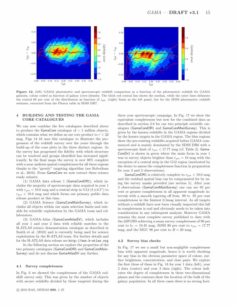
training set is composed of all GAMA spectroscopic redshiftsand zCOSMOS spectroscopic redshift (Lilly et al. 2007), aswell as the 30-band COSMOS photometric redshifts (Ilbertet al. 2009). With a redshift error of < 0.001, these are asgood as spectroscopy when it comes to calibrating 5-bandphoto-z’s from SDSS alone. The corresponding fractions inthe training, validating and testing sets are 81 per cent, 4per cent and 15 per cent respectively, with over 120k galax-ies in total. For COSMOS (and hence zCOSMOS) galaxies,we perform a careful matching to SDSS DR7 objects. Thislarge, complete, and representative photo-z training set al-lows us to use an empirical regression method to estimatethe errors on individual photometric redshifts. The left panelof Fig. 12 shows that up to zph ≈ 0.40 the bias in the medianrecovered photo-z is less than 0.005/(1+ zph), while beyondit (not shown) the bias is typically within 0.01/(1 + zph).Considering the random errors on the individual estimates,this systematic bias is negligible, while still very well quan-tified. The right panel of Fig. 12 presents the equivalent plotusing SDSS DR7 photometric redshifts, as listed in the Pho-toz table of the SDSS Sky Server. In both cases, these plotsshow only galaxies with rpet < 19.8 mag. This comparison

Figure 13. Spectroscopic redshift distribution of GAMA galax-ies (black), the corresponding photo-z distribution of GAMA

galaxies (red) and one thousand Monte-Carlo generated photo-zdistributions, including the Gaussianly distributed photo-z error(green).

highlights the importance of using a complete and fully rep-resentative sample in the training of photometric redshifts.

For an extensive and complete training set such asGAMA, it is possible to derive a simple and direct methodfor calculating photo-z errors. We estimate the photo-z ac-curacy in a rest-frame colour magnitude plane with severalhundreds of objects per 0.1×0.1 mag bin down to rpet = 19.8mag, and typically about fifty objects per 0.1× 0.1 mag bindown to rpet ≈ 21.5 mag. This method provides a robustnormally distributed error for each individual object. Wenote that with this realistic photo-z error it is possible to cor-rectly recover the underlying spectroscopic redshift distribu-tion with our ANNz photometric redshifts as illustrated inFig. 13. It is interesting to note that, without this added er-ror, the raw photo-z histogram is actually narrower than thespectroscopic histogram. This makes sense, because photo-zcalibration yields no bias in true z at given zphot: it is thusinevitable that there is a bias in zphot at given true z, whichis strong wherever N(z) changes rapidly; this effect can beseen in operation in the ranges z < 0.05 and 0.3 < z < 0.5.GamaPhotoz contains both photometric redshifts and errorsfor all systems to rmodel < 21.5 mag and the code is cur-rently being applied across the full SDSS region. We plan torelease our prescription for these improved all-SDSS photo-z’s by the end of 2010. In the meantime, we are open to col-laborative use of the data: contact [email protected].

c© 2010 RAS, MNRAS 000, 1–27


Figure 12. (left) GAMA photometric and spectroscopic redshift comparison as a function of the photometric redshift for GAMAgalaxies, colour coded as function of galaxy (over-)density. The thick red central line shows the median, while the outer lines delineatethe central 68 per cent of the distribution as function of zph. (right) Same as the left panel, but for the SDSS photometric redshiftestimate, extracted from the Photoz table in SDSS DR7.

4 BUILDING AND TESTING THE GAMACORE CATALOGUES

We can now combine the five catalogues described aboveto produce the GamaCore catalogue of ∼ 1 million objects,which contains what we define as our core product to r < 22mag. Figs 14–16 uses this catalogue to illustrate the pro-gression of the redshift survey over the years through thebuild-up of the cone plots in the three distinct regions. Asthe survey has progressed the fidelity with which structurecan be resolved and groups identified has increased signif-icantly. In the final maps the survey is over 98% completewith a near uniform spatial completeness for all three regionsthanks to the “greedy” targeting algorithm (see Robothamet al., 2010). From GamaCore we now extract three scienceready subsets:

(1) GAMA data release 1 (GamaCoreDR1), which in-cludes the majority of spectroscopic data acquired in year 1with rpet < 19.0 mag and a central strip in G12 (δ±0.5) torpet < 19.8 mag and which forms our primary public datarelease product at this time.

(2) GAMA Science (GamaCoreMainSurvey), which in-cludes all objects within our main selection limits and suit-able for scientific exploitation by the GAMA team and col-laborators.

(3) GAMA-Atlas (GamaCoreAtlasSV), which includesall year 1 and year 2 data with reliable matches to theH-ATLAS science demonstration catalogue as described inSmith et al. (2010) and is currently being used for scienceexploitation by the H-ATLAS team. For further details andfor the H-ATLAS data release see http://www.h-atlas.org

In the following section we explore the properties of thetwo primary catalogues (GamaCoreDR1 and GamaCoreMain-

Survey) and do not discuss GamaAtlasSV any further.

4.1 Survey completeness

In Fig. 6 we showed the completeness of the GAMA red-shift survey only. This was given by the number of objectswith secure redshifts divided by those targeted during the

three year spectroscopic campaign. In Fig. 17 we show theequivalent completeness but now for the combined data asdescribed in section 2.8 for our two principle scientific cat-alogues (GamaCoreDR1 and GamaCoreMainSurvey). This isgiven by the known redshifts in the GAMA regions dividedby the known targets in the GAMA region. The blue regionsshow the pre-existing redshifts acquired before GAMA com-menced and is mainly dominated by the SDSS DR6 with aspectroscopic limit of rpet < 17.77 mag (cf. Table 2). Gama-

CoreDr1 is shown in green where the main focus in year 1was to survey objects brighter than rpet = 19 mag with theexception of a central strip in the G12 region (motivated bythe desire to assess the completeness function in preparationfor year 2 and 3 observations).

GamaCoreDR1 is relatively complete to rpet < 19.0 magand the residual spatial bias can be compensated for by us-ing the survey masks provided (see section 5). After year3 observations (GamaCoreMainSurvey) one can see 95 percent or greater completeness in all apparent magnitude in-tervals with a smooth tapering off from 99 to 95 per centcompleteness in the faintest 0.5mag interval. As all targetswithout a redshift have now been visually inspected this fallin completeness is real and obviously needs to be taken intoconsideration in any subsequent analysis. However GAMAremains the most complete survey published to date withthe 2dFGRS achieving a mean survey completeness of 90 percent to bJ = 19.45 mag, SDSS 90 per cent to rpet = 17.77mag, and the MGC 96 per cent to B = 20 mag.

4.2 Survey bias checks

In Fig. 17 we see a small but non-negligible completenessbias with apparent magnitude, hence it is worth checkingfor any bias in the obvious parameter space of colour, sur-face brightness, concentration, and close pairs. We explorethe first three of these in Fig. 18 for year 1 data (left), year2 data (centre) and year 3 data (right). The colour indi-cates the degree of completeness in these two-dimensionalplanes and the contours show the location of the bulk of thegalaxy population. In all three cases there is no strong hori-

c© 2010 RAS, MNRAS 000, 1–27

http://www.h-atlas.org


Figure 14. Redshift cone diagram for the GAMA 09 region showing (top to bottom), pre-existing data, year 1 data release added, year2 data release added, year 3 data release added.

zontal bias that would indicate incompleteness with colour,surface brightness, or concentration. This is not particularlysurprising given the high overall completeness of the sur-vey, which leaves little room for bias in the spectroscopicsurvey, but we acknowledge the caveat that bias in the in-put catalogue cannot be assessed without deeper imagingdata. Note that in these plots surface brightness is definedby: µeff = rpet + 2.5 log10(2πab) where a and b are the ma-jor and minor half-light radii as derived by GALFIT3 (seeKelvin et al. 2010 in prep, for details of the fitting process)

and concentration is defined by log10(n) where n is the Sersicindex derived in section 3.2.

A major science priority of the GAMA programme isto explore close pairs and galaxy asymmetry (e.g., De Pro-pris et al. 2007). As GAMA is a multi-pass survey with eachregion of sky being included in 4-6 tiles (see. Fig. 2), theclose pair biases due to minimum fibre separations, whichplague the 2dFGRS, SDSS, and MGC studies, are over-come. Fig. 19 shows the redshift completeness versus neigh-bour class. The neighbour class of any galaxy is defined (seeBaldry et al. 2010) as the number of target galaxies within a

c© 2010 RAS, MNRAS 000, 1–27



40′′ radius. The nominal 2dF fibre-collision radius. The fig-ures shows the progress towards resolving these complexesat the outset and after each year the survey has been op-erating. All low neighbour class objects are complete withonly a few redshifts outstanding in a small fraction of thehigher neighbour class complexes. The data therefore rep-resents an excellent starting point for determining mergerrates via close pair analyses.

4.3 Overdensity/underdensity of the GAMAregions

All galaxy surveys inevitably suffer from cosmic variance,more correctly stated as sample variance. Even the finalSDSS, the largest redshift survey to date, suffers an esti-mated residual 5 per cent cosmic variance to z < 0.1 (seeDriver & Robotham 2010) — mainly attributable to the“Great Wall” (see Baugh et al. 2004; Nichol et al. 2006).As the GAMA regions lie fully within the SDSS it is possi-ble to determine whether the GAMA regions are overdenseor underdense as compared to the full SDSS over the un-

c© 2010 RAS, MNRAS 000, 1–27



biased redshift range in common (z < 0.1) and relative toeach other at higher redshifts where the SDSS density dropsdue to incompleteness imposed by the rpet < 17.77 magspectroscopic limit. Fig. 20 shows results with the upperpanel showing the density of M∗ ± 1.0 galaxies (defined asM∗ − 5 log h = −20.81 mag) in 0.01 redshift intervals, fora 5000 sq.deg. region of the SDSS DR7 (blue), and for thethree GAMA blocks (as indicated) and the sum of the threeregions (solid black histogram). The k and e correctionsadopted and the methodology, including the SDSS sampleconstruction, are described in Driver & Robotham (2010)

but are not particularly important as we are not exploringtrends with z but rather the variance at fixed z. The errorbars shown are purely Poisson and so discrepancies largerthan the error bars are indicative of cosmic variance inducedby significant clustering along the line-of-sight. The middleand lower panels show the sum of these density fluctuationsrelative to either SDSS (middle) or the average of the threeGAMA fields (lower). Note that these panels (middle, lower)now show the density fluctuation out to the specified redshiftas opposed to at a specific redshift (top), i.e., the cosmic vari-ance. We can see that out to z = 0.1 the three GAMA fields

c© 2010 RAS, MNRAS 000, 1–27


Figure 17. The final completeness of the combined redshift catalogues prior to survey commencing (blue), after GamaCoreDR1 (green)and GamaCoreMainSurvey (red) for G09, G12 and G15 (left to right). In all cases the solid black lines shows 95 per cent completeness.

Figure 19. The redshift completeness as a function of NeighbourClass (NC). NC is defined for each target as the number of otherMain Survey targets within 40′′ (numbers with each NC valueare annotated in the figure). The various lines show the progressin resolving clustered objects at the outset and after each year ofobservations for the r-limited Main Survey. Note the bias towardNC>0 after Year 1 and 2 is the result of increasing the priorityof clustered targets (Robotham et al. 2010) in order to avoidbeing biased against NC>0 after Year 3. The final survey hasfully resolved almost all close complexes leaving only a minimalbias when determining merger rates via close pairs: the redshiftcompleteness is > 95% for NC ≤ 5.

are overall 15 per cent under dense with respect to a 5000sq.deg. region of SDSS DR7 (NB: the volume surveyed bythe SDSS comparison region is ∼ 1.3 × 107h−3Mpc3). Thisis extremely close to the 15 per cent predicted from Table 2of Driver & Robotham (2010). Beyond z = 0.1 one can onlycompare internally between the three GAMA fields. The in-ference from Fig. 20 is that for any study at z < 0.2 thecosmic variance between the three regions is significant withG09 in particular being under-dense for all redshifts z < 0.2when compared to the other two regions (NB: the volumesurveyed within the combined GAMA regions to z < 0.2 is∼ 2.8×106h−3Mpc3). It is therefore important when consid-ering any density measurement from GAMA data to includethe cosmic variance errors indicated in Fig. 20. For examplea luminosity function measured from the G09 region onlyout to z = 0.1 would need to be scaled up by ×1.41 etc.

5 MASKS

For accurate statistical analysis of GAMA it is essentialto have a full understanding of the criteria that defineits parent photometric catalogue, and also of the spatialand magnitude-dependent completeness of the redshift cat-alogue. For this purpose we have defined three functionscharacterizing this information as a function of position onthe sky and magnitude selection. Here we present briefly thetwo most important ones, i.e. the survey imaging mask func-tion and the redshift completeness mask relative to the mainrpet survey limits. The combination of both functions is keyfor any spatially dependent measurements based on GAMAdata, and in particular on GAMA year 1 data. Additional

c© 2010 RAS, MNRAS 000, 1–27


Year 10

24

68

10

u pet

−r p

et

Year 2 Year 314

1822

26

µ(m

ags

arcs

ec2 )

13 14 15 16 17 18 19 20

−1.

00.

00.

51.

0

rpet

log(

N)

14 15 16 17 18 19 20

rpet

14 15 16 17 18 19 20

rpet

0.0

0.2

0.4

0.6

0.8

1.0

Comp

Figure 18. Completeness is the bivariate planes of apparent magnitude and u−r colour (top), apparent magnitude and effective surfacebrightness (middle), apparent magnitude and Sersic index (bottom) for GAMA data after year 1 (left), year 2 (centre) and year 3 (right).Contours show the percentage of galaxies enclosed from out to in 99, 95, 75, 50 & 5 per cent. Apart from the progression in apparentmagnitude over the three years no other obvious bias is evident.

survey completeness masks for other selections (e.g., z, K)or any combination of are available to the Team and will bereleased shortly.

5.1 The imaging mask

We are interested in knowing which regions of the GAMAareas have not been properly covered by the SDSS imagingsurvey, or which should be excluded owing to the presenceof bright stars. For that reason, we want to map out SDSSimaging areas containing any of the following information:bleeding pixel, bright star, satellite trail or hole.

First we create, following the imaging mask informationavailable on the SDSS DR6 website3, the associated convex

3 http://www.sdss.org/dr6/products/images/use masks.html

and http://www.sdss.org/dr6/algorithms/masks.html

polygons, delimiting areas for which imaging information iseither not available or could be corrupted (as in the case ofbleeding pixels). We primarily use the r-band imaging maskinformation, as GAMA is nominally an r-band selected sur-vey, but for completeness we construct all five SDSS imagingmasks for the GAMA areas.

Then we build an additional bright star mask based onstars down to V < 12 in the Tycho 2, Tycho 1 and Hipparcoscatalogues. For each star we define an exclusion radius r,defined as:

r = Rs/0.8 for 10 < V ≤ 12 (2)

r = Rs/0.5 for V ≤ 10 (3)

where Rs is the scattered-light radius, as estimated basedon the circular region over which the star flux per pixel isgreater than five times the sky noise level. Further details

c© 2010 RAS, MNRAS 000, 1–27

http://www.sdss.org/dr6/products/images/use_masks.html

http://www.sdss.org/dr6/algorithms/masks.html


Figure 21. Spatial completeness masks to rpet < 19.0 mag after year 1 (left) and year 3 (right). The three GAMA regions are shownfrom top to bottom as G09, G12 and G15. The white regions indicate areas not sample either due to missing input catalogue data orbright stars.

0 0.05 0.1 0.15 0.2 0.250.001

0.01

All (GAMA) G09 G12 G15 SDSS DR7

0 0.05 0.1 0.15 0.2 0.25

406080

100120140160

Overdensity w.r.t. SDSS DR7

0 0.05 0.1 0.15 0.2 0.25

406080

100120140160

Redshift

Overdensity w.r.t. All GAMA

Figure 20. (upper) The differential number-density of M∗ ± 1.0mag galaxies in redshift intervals of 0.01. (middle) the overdensityof M∗ ± 1.0 mag galaxies out to the specified redshift for thesurvey indicated by line colour relative to that seen in a 5000sq.deg. region of SDSS DR7. (lower) the overdensity of M∗ ± 1.0mag galaxies out to the specified redshift for the survey indicatedrelative to that seen over all three GAMA regions.

on the bright star exclusion mask are given in section 3.3 ofBaldry et al. (2010).

The final imaging mask function is then the union of thetwo separate functions. For ease of use, the imaging maskshave been pixelated using an equal area projection.

5.2 The rpet redshift completeness mask

Normally a simple way to define a redshift success rate wouldbe to make use of the geometry defined by the complete setof 2 fields that were used to tile the survey region for spec-troscopic observations. However, due to the tiling strategyadopted in the first year, due to the preselection of observingthe brightest targets first, and due to the much higher num-ber density of galaxies than can be accommodated in a sin-gle 2dF field, this simple and straightforward approach doesnot account well enough for the spatial incompleteness of thesurvey. Therefore for year 1 data, we had to develop differentcompleteness masks each defined for a different magnitudelimit interval:

• For G09 and G15, there are two completeness maskseach: one for galaxies brighter than rpet = 19.0 and one for19.0 ≤ rpet < 19.4.

• For G12, there are three completeness masks: the sametwo as for G09 and G15, as well as one for 19.4 ≤ rpet < 19.8.

Once the samples for which completeness masks areneeded have been defined, one just needs to provide a rea-sonable definition for the redshift success rate. We choose totessellate the GAMA regions with a large number of sectors.We incorporate the relevant imaging mask at this stage, byimposing that sectors do not cover any regions masked bythe imaging mask. Each sector contains between 15 and 50galaxy targets, is limited in extent (less than 24 arcmin)and in size (less than 225 arcmin2). These conditions arenecessary to avoid shot-noise dominated masks, and to guar-antee that small scale information is preserved as much aspossible. We note that in the current implementation these

c© 2010 RAS, MNRAS 000, 1–27


sectors are not uniquely defined,4 but once specified anygiven position on the sky belongs to a unique sector. Foreach sector, θ, we define the redshift success rate, Rz(θ), fora sample of galaxies within specified magnitude limits, asthe ratio of the number of galaxies for which good qualityredshifts have been obtained, Nz(θ), to the total numberof objects contained in the tiling catalogue, Nt(θ). The red-shift completeness of a given sector, Rz(θ), should be clearlydistinguished from the redshift completeness of a given 2dFfield, cF , since multiple overlapping fields can contribute toa single sector and cF is a measure of the quality of theobserving conditions for galaxies observed at the same time.

We present in Fig. 21 the completeness masks for allthree regions for GamaCoreDR1 (left) and GamaCoreMain-Survey (right) to rpet < 19.0. Completeness masks for allregions and different selections are available to the teammembers and collaborators only at this stage.

6 GAMA SCIENCE READY CATALOGUESAND DATA RELEASE 1

The combination of our five input catalogues, as outlinedin section 4, constitutes our core GAMA catalogue of ∼ 1million galaxies lying within the GAMA regions and extend-ing to approximately rpet < 22.0 mag. This catalogue hasinhomogeneous selection, is liable to be incomplete towardsthe faint-end, along with significant noise in the photometryat the very faint limit and spurious detections. We thereforeextract from this dataset three science-ready catalogues andone overflow catalogue. These four catalogues along with thecomplete SWARP’ed mosaics of the GAMA regions, associ-ated spectra bundles, images, Sersic profiles and a varietyof data inspection tools (including a MySQL access point)constitute our first data release and are now available via:http://www.gama-survey.org/

6.1 GamaCoreMainSurvey - Available 01/07/12

The GamaCoreMainSurvey is the GAMA team’s principal sci-ence catalogue and is constructed from GamaCore by remov-ing all objects outside our Main Survey limits as defined inBaldry et al. (2010). These limits are: rpet < 19.4 mag inG09 & G15 and rpet < 19.8 mag in G12 (114 441 objects).KKron < 17.6 with rmodel < 20.5 mag (61393 objects) orzModel < 18.2 with rmodel < 20.5 mag (55534 objects) andare selected using SURVEY CLASS> 3. For a description ofthe SURVEY CLASS parameter see Table 3). This amountsto 119 778 objects in total of which 101 576 are new redshiftsprovided by GAMA and 18202 pre-existing. Fig. 17 showsthe completeness in the r-band however similar plots cantrivially be constructed in z or K. The spectroscopic com-pleteness (which includes objects not targeted) is 98.2 percent in r, 99.3 per cent in z and 98.6 per cent in K. The pa-rameters contained in this catalogue are listed in Table A2.As this is our main science catalogue we place an embargoon its public release until 1st July 2012 but are open torequests for collaboration sent to: [email protected]

4 This could be achieved by making each target galaxy the centreof a subsector and then increasing the radius of all subsectors andcreate sectors by the merger of overlapping subsectors.

130 132 134 136 138 140

−1

01

23

RA

DE

C

GAMANon−GAMA

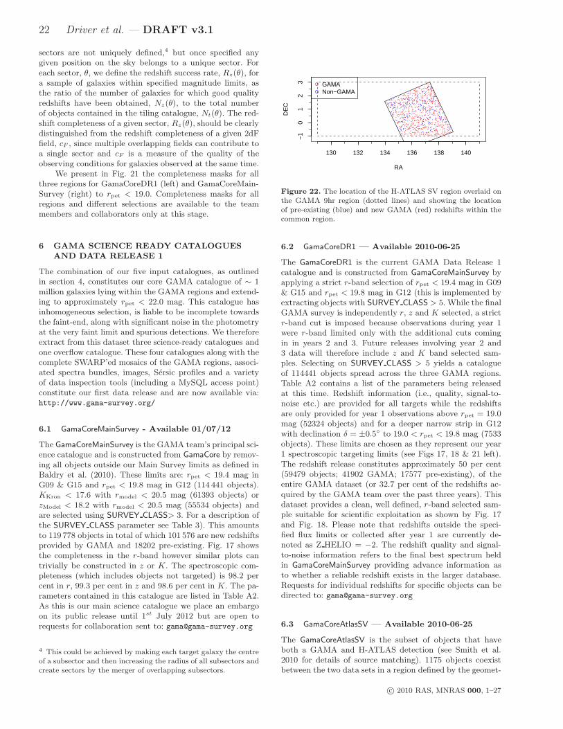
Figure 22. The location of the H-ATLAS SV region overlaid onthe GAMA 9hr region (dotted lines) and showing the locationof pre-existing (blue) and new GAMA (red) redshifts within thecommon region.

6.2 GamaCoreDR1 — Available 2010-06-25

The GamaCoreDR1 is the current GAMA Data Release 1catalogue and is constructed from GamaCoreMainSurvey byapplying a strict r-band selection of rpet < 19.4 mag in G09& G15 and rpet < 19.8 mag in G12 (this is implemented byextracting objects with SURVEY CLASS > 5. While the finalGAMA survey is independently r, z and K selected, a strictr-band cut is imposed because observations during year 1were r-band limited only with the additional cuts comingin in years 2 and 3. Future releases involving year 2 and3 data will therefore include z and K band selected sam-ples. Selecting on SURVEY CLASS > 5 yields a catalogueof 114441 objects spread across the three GAMA regions.Table A2 contains a list of the parameters being releasedat this time. Redshift information (i.e., quality, signal-to-noise etc.) are provided for all targets while the redshiftsare only provided for year 1 observations above rpet = 19.0mag (52324 objects) and for a deeper narrow strip in G12with declination δ = ±0.5 to 19.0 < rpet < 19.8 mag (7533objects). These limits are chosen as they represent our year1 spectroscopic targeting limits (see Figs 17, 18 & 21 left).The redshift release constitutes approximately 50 per cent(59479 objects; 41902 GAMA; 17577 pre-existing), of theentire GAMA dataset (or 32.7 per cent of the redshifts ac-quired by the GAMA team over the past three years). Thisdataset provides a clean, well defined, r-band selected sam-ple suitable for scientific exploitation as shown by Fig. 17and Fig. 18. Please note that redshifts outside the speci-fied flux limits or collected after year 1 are currently de-noted as Z HELIO = −2. The redshift quality and signal-to-noise information refers to the final best spectrum heldin GamaCoreMainSurvey providing advance information asto whether a reliable redshift exists in the larger database.Requests for individual redshifts for specific objects can bedirected to: [email protected]

6.3 GamaCoreAtlasSV — Available 2010-06-25

The GamaCoreAtlasSV is the subset of objects that haveboth a GAMA and H-ATLAS detection (see Smith et al.2010 for details of source matching). 1175 objects coexistbetween the two data sets in a region defined by the geomet-

c© 2010 RAS, MNRAS 000, 1–27



Table 3. The survey class parameter given in GamaTiling. Objects take the higher value if satisfying more than one criteria. All objectswith survey class ≥ 2 pass the standard star-galaxy separation. See Baldry et al. (2010) for details.

value number frac.Q ≥ 3 criteria and notes

7 59756 0.995 rpet < 19.0 and ∆sg > 0.25 (high priority in Year 1)

6 54685 0.968 rpet < 19.4 or rpet < 19.8 in G12 (≥ 6 for r-limited Main Survey)5 1386 0.703 zmodel < 18.2 (≥ 5 for SDSS-mag limited Main Survey)4 3951 0.879 KAB < 17.6 (≥ 4 for Main Survey)3 33134 0.343 19.4 < rpet < 19.8 in G09 or G15 (F2 fillers)2 14861 0.196 gmodel < 20.6 or rmodel < 19.8 or imodel < 19.4 in G12 (F3 fillers)1 1255 0.577 radio selected targets (F1 fillers, Ching et al. in preparation)0 822 0.394 2 ≤ vis class ≤ 4 or fails star-galaxy separation for rfib < 17

Figure 23. (Main panel). The absolute magnitude versus red-shift plane for the three science ready catalogues (as indicated).(left) the distribution collapsed in redshift, (upper) the distribu-tion collapsed in absolute magnitude.

ric overlap between G09 and the H-ATLAS SV region (seeFig. 22), with an approximate area of ∼ 16.7 deg2. Using theGamaCoreMainSurvey catalogue we find ∼ 15 per cent ofGAMAMain Survey targets have a H-ATLAS source match.Of these matches 89 do not have any available redshift, 306have SDSS redshifts, 792 have GAMA redshifts and 1 objecthas a 2SLAQ-QSO redshift. The GAMA redshifts compriseof 523 year 1 redshifts, 182 year 2 redshifts and 87 year 3redshifts. There are no magnitude cuts imposed for Gama-

CoreAtlasSV and therefore 178 of these redshifts derive fromGamaCoreExtra. Note that to extract a homogeneously se-lected sample one must trim this catalogue to rpet < 19.4mag. Table A3 shows the parameters included in this cata-logue.

6.4 GamaCoreExtraDR1 — Available 2010-06-25

The GamaCoreExtra catalogue contains information on allobjects for which redshifts are known but lie outsidethe GamaCoreDR1 selection limits. In effect GamaCoreEx-

tra serves as a redshift dumping ground and when com-

bined with GamaCoreMainSurvey or GamaCoreDR1 providesa full record of all objects with known redshifts in the threeGAMA regions. This will include pre-existing redshifts atfaint magnitudes in the public domain (predominantly fromQSO and LRG surveys), along with filler objects targetedduring the GAMA campaign. The parameters included areidentical to GamaCoreDR1 and therefore also described inTable A2. GamaCoreExtraDR1 is an identical copy of Gama-

CoreExtra except with the GAMA redshifts embargoed un-til a later release. GamaCoreExtra is highly inhomogeneousand volatile as additional redshifts come to light and es-sentially forms the starting point for any extension to theGAMA survey. Currently it contains ∼ 16k galaxies of which∼ 0.5k are pre-existing and ∼ 15.5k have been acquired dur-ing GAMA observations. Requests for access to individualredshifts or redshifts for specified sub-regions should be di-rected to: [email protected]

6.5 Future plans

The three science ready catalogues described in the previoussections are shown in Fig. 23 in the Absolute r-band mag-nitude (Mr −5 log h) versus redshift (z) plane (main panel),along with the collapsed N(z) and N(Mr) distributions (up-per and right panels respectively). The absolute magnitudesare calculated using k-corrections derived from the GAMAu to K photometry, and total throughput (including atmo-sphere) temperature adjusted filter transmission curves, andthe KCORRECT software package (Blanton & Roweis 2007).The figure is intended to provide a rough indication of theparameter range being explored with L∗ galaxies routinelydetected to z ≈ 0.3 and objects as faint as Mr = −12 magbeing recovered at z > 0.01. In future papers we will ex-plore more comprehensively the completeness of the initialinput catalogue (GamaTiling) in the bivariate brightness dis-tribution plane (BBD; Hill et al. 2010, in prep.,) througha detailed BBD-analysis (see Driver et al. 2005), as well asthrough comparisons to deeper and higher spatial resolutiondata.

In the near term the GAMA team will be produc-ing a number of extended data products or data manage-ment units (DMUs), which include: spectral line analysis viaGANDALF/ppxf (Sarzi et al., 2006; Cappellari & Emsellem2004) and stellar population model fits (Maraston 2005;Thomas, Maraston & Bender 2003), bulge-disc decompo-sition via GALFIT3, stellar masses and revised photometric-redshifts via INTEREST, environmental markers, and groupcatalogues. These data products will be outlined in moredetail in our next data release later in the year (Liske et

c© 2010 RAS, MNRAS 000, 1–27


al., 2010, in prep.). Within the next 3—5 years we expectto ingest additional datasets from GALEX, HERSCHEL,WISE, GMRT, VISTA, VST, and ASKAP as well as ex-pand our core AAT programme to cover a larger area of∼ 400 sq deg. to rSersic < 19.8 mag. In due course DMUson multiwavelength SED and HI modeling will provide dustmass/temperature measurements, and gas and dynamicalmass measurements.

7 SUMMARY

The GAMA basic-data including GAMA and pre-GAMAspectra and redshifts, GAMA SWARP processed imagesin ugrizY JHK, u to K matched aperture photometry,corrections to total magnitudes are now available at:http://www.gama-survey.org/. GAMA Data Release 1(GamaCoreDR1) data is publicly available via a downloadspage immediately, and the full catalogue (GamaCoreMain-

Survey) is available for use by the GAMA team and collab-orators. In addition we make publicly available a catalogue(GamaCoreAtlasSV) including year-2 data for the H-AtlasScience Verification region, which form the basis for a num-ber of H-Atlas Science Verification papers.

Data inspections tools, including a MySQL tool and di-rect data inspection toolkit, are provided and will be devel-oped further in due course. The sum of year 1, 2, and 3 dataconstitutes GAMA Phase I, which is now complete havingutilised archival data from the Sloan Digital Sky Survey, theUK Infrared Deep Sky Survey, and the NASA ExtragalacticDatabase and an initial allocation of 66 nights of Anglo-Australian Telescope time. Value added data products willbe released from January 1st 2011 and regularly thereafter.GAMA Phase II is now underway and aims to add in ad-ditional area coverage as well as to extend the depth of thesurvey. The community is encouraged and invited to con-tact the team for early access to GamaCoreMainSurvey. Thecontents of this catalogue are described in Table A2.

ACKNOWLEDGMENTS

First and foremost we would like to thank the staff of theformer Anglo-Australian Observatory (now Australian As-tronomical Observatory), for the the smooth running of thetelescope and AAOmega during these observations and thefunding support we have received from the STFC and theARC.

Funding for the SDSS and SDSS-II has been providedby the Alfred P. Sloan Foundation, the Participating In-stitutions, the National Science Foundation, the U.S. De-partment of Energy, the National Aeronautics and SpaceAdministration, the Japanese Monbukagakusho, the MaxPlanck Society, and the Higher Education Funding Councilfor England. The SDSS Web Site is http://www.sdss.org/.The SDSS is managed by the Astrophysical Research Con-sortium for the Participating Institutions. The Participat-ing Institutions are the American Museum of Natural His-tory, Astrophysical Institute Potsdam, University of Basel,University of Cambridge, Case Western Reserve Univer-sity, University of Chicago, Drexel University, Fermilab,the Institute for Advanced Study, the Japan Participation

Group, Johns Hopkins University, the Joint Institute forNuclear Astrophysics, the Kavli Institute for Particle As-trophysics and Cosmology, the Korean Scientist Group, theChinese Academy of Sciences (LAMOST), Los Alamos Na-tional Laboratory, the Max-Planck-Institute for Astronomy(MPIA), the Max-Planck-Institute for Astrophysics (MPA),New Mexico State University, Ohio State University, Uni-versity of Pittsburgh, University of Portsmouth, PrincetonUniversity, the United States Naval Observatory, and theUniversity of Washington.

The UKIDSS project is defined in Lawrence et al.(2007). UKIDSS uses the UKIRT Wide Field Camera (WF-CAM; Casali et al, 2007). The photometric system is de-scribed in Hewett et al. (2006), and the calibration is de-scribed in Hodgkin et al. (2009). The pipeline processingand science archive are described in Irwin et al. (2009, inprep) and Hambly et al. (2008). We have used data fromthe 4th data release.

This research has made use of the NASA/IPAC Ex-tragalactic Database (NED), which is operated by the JetPropulsion Laboratory, California Institute of Technology,under contract with the National Aeronautics and SpaceAdministration.

The Millennium Galaxy Catalogue consists of imag-ing data from the Isaac Newton Telescope and spectro-scopic data from the Anglo Australian Telescope, theANU 2.3m, the ESO New Technology Telescope, the Tele-scopio Nazionale Galileo and the Gemini North Tele-scope. The survey has been supported through grantsfrom the Particle Physics and Astronomy Research Coun-cil (UK) and the Australian Research Council (AUS).The data and data products are publicly available fromhttp://www.eso.org/~jliske/mgc/ or on request from J.Liske or S.P. Driver.

Finally we would like to acknowledge the use of Topcat,Stilts, SExtractor, SWARP, PSFex, GALFIT3 and ALADINastronomical software packages and the r data analysis pack-age.

APPENDIX A: GAMA CATALOGUES

The four principle GAMA catalogues formed at this timeare: GamaTiling, GamaCoreMainSurvey, GamaCoreDR1 andGamaCore AtlasSv. The parameters contained in these cata-logues and their explanations are showing in Tables. A1—A3respectively.

c© 2010 RAS, MNRAS 000, 1–27


http://www.sdss.org/

http://www.eso.org/\protect \protect \protect \edef OT1OT1\let \enc@update \relax \protect \edef cmttcmr\protect \edef mm\protect \edef nn\protect \xdef \OT1/cmtt/m/n/9 \OT1/cmtt/m/n/9 \OT1/cmtt/m/n/9 \size@update \enc@update \ignorespaces \relax \protect \relax \protect \edef cmttcmtt\protect \xdef \OT1/cmtt/m/n/9 \OT1/cmtt/m/n/9 \OT1/cmtt/m/n/9 \size@update \enc@update ~jliske/mgc/


Table A1. Parameters held in GamaTiling

Column Parameter Units Definition

1 GAMA ID N/A Unique six digit GAMA identifier linked to GAMAs original SDSS DR6 input cat2 SDSS ID N/A Sloan Identifier from SDSS DR63 RA J2000 Degrees RA taken from SDSS DR64 DEC J2000 Degrees Declination taken from SDSS DR65 r FIBREMAG AB mag Fibre magnitude6 r PETRO AB mag Extinction corrected r-band Petrosian flux derived from SDSS DR67 u MODEL AB mag Extinction corrected model u mag from SDSS DR68 g MODEL AB mag Extinction corrected model g mag from SDSS DR69 r MODEL AB mag Extinction corrected model r mag from SDSS DR610 i MODEL AB mag Extinction corrected model i mag from SDSS DR611 z MODEL AB mag Extinction corrected model z mag from SDSS DR612 NUM GAMA SPEC N/A Number of spectra available for this object13 r SB AB mag arcsec−2 SDSS Petro half-light r-band surface brightness14 SG SEP mag SDSS r psf-r model star-galaxy separation parameter15 SG SEP JK mag GAMA AUTO J-K - f locus star-galaxy separation parameter16 K KRON SELECTION AB mag Extinction corrected K magnitude used for selection (Old)17 TARGET FLAGS bit bitwise target criteria (see gama website)18 SURVEY CLASS N/A Survey class (see Table 3)19 PRIORITY CLASS N/A Priority class (see gama website)20 NEIGHBOUR CLASS N/A Number of Main Survey neighbours within 40 arcseconds (see Fig. 19)21 MASK IC 10 N/A Mask value 0.0 to 1.0 around V < 10 mag stars (see Baldry et al. 2010)22 MASK IC 12 N/A Mask value 0.0 to 1.0 around V < 12 mag stars (see Baldry et al. 2010)23 VIS CLASS N/A Visual classification (see Baldry et al. 2010)24 VIS CLASS USER N/A Initials of visual classifier for VIS CLASS

REFERENCES

Adelman-McCarthy J.K., et al., 2008, ApJS, 175, 297

Allen P.D., Driver S.P., Graham A.W., Cameron E., LiskeJ., De Propris R., 2006, MNRAS, 371, 2

Abazajian K.N., et al., 2009, ApJS 182, 543

Baldry, I.K., et al., 2010, MNRAS, 404, 86

Baldry I.K., Balogh M.L., Bower R.G., Glazebrook K.,Nichol R.C., Bamford S.P., Budavari T., 2006, MNRAS,373, 469

Baugh C.M., et al., 2004, MNRAS, 351, 44

Belokurov V., et al., 2006, ApJ, 642, 137

Bell E.F., McIntosh D.H., Katz N., Weinberg M.D., 2003,ApJS, 149, 289

Bell E.F., Phleps S., Somerville, R.S., Wolf, C., Borch A.,Meisenheimer, K., 2006, ApJ, 652, 270

Bertin E., Arnouts S., 1996, A&AS, 117, 393

Bertin E., Mellier Y., Radovich M, Missonnier G, DidelonP, Morin B, 2002, in ASP Conf. Proc on AstronomicalData Analysis Software and Systems (Eds. David A.Bohlender, Daniel Durand & Thomas H. Handley), 281,228

Blanton M.R., Roweis, S., 2007, AJ, 113, 734

Bower R.G., Benson A.J., Malbon R, Helley J.C., FrenkC.S., Baugh C.M., Cole S.G., Lacey C.G., 2006, MN-RAS, 370, 645

Canon R., et al., 2006, MNRAS, 372, 425

Cameron E., Driver S.P., 2007, MNRAS, 377, 523

Cappellari M., Emsellem E., 2004, PASP, 116, 138

Choi Y-Y, Park Changbom, Vogeley M.S., 2007, ApJ, 638,87

Cole S., et al., 2005, MNRAS, 362, 505

Colless M., et al., 2001, MNRAS, 328, 1039

Colless M., et al., 2003, arXiv:astro-ph/0306581

Collister A.A., Lahav O., 2004, PASP, 116, 345

Cook M., Barausse E., Evoli C., Lapi A., Granato G.L.,2010, MNRAS, 402, 2113

Croom S., Saunders W., Heald R., 2004, AAO Newsletter,106, 12

Croom S.M., Smith R.J., Boyle B.J., Shanks T., Miller L.,Outram P.J., Loaring N.S., 2004, MNRAS, 349, 1397

Croom S.M., et al., 2009, MNRAS, 392, 19

De Lucia G., Springer V., White S.D.M., Croton D., Kauff-mann G., 2006, MNRAS, 366, 499

De Propris R, Conselice C.J., Liske J., Driver S.P., PattonD.R., Graham A.W., Allen P.D., 2007, ApJ, 666, 212

Driver, S.P., Liske J., Cross N.J.G., De Propris R., AllenP.D., 2005, MNRAS, 360, 81

Driver S.P., et al., 2006, MNRAS, 368, 414

Driver S.P., Popescu C.C., Tuffs R.J., Liske J., GrahamA.W., Allen P.D., De Propris, R, 2007, MNRAS, 379,1022

Driver S.P., Popescu C.C., Tuffs R.J., Graham A.W., LiskeJ., Baldry I., 2008, ApJ, 678, 101

Driver S.P., et al., 2009, A&G, 50, 12

Driver S.P., Robotham A.S.G., 2010, MNRAS, in press(arXiv:1005.2538)

Eales, S., et al., 2010, PASP, 122, 499

Eke V.R., et al., 2004, MNRAS, 348, 866

Falco E.E., et al., 1999, PASP, 111, 438

Gadotti, D.A., 2009, MNRAS, 393, 1531

Graham A.W., Driver S.P., 2005, PASA, 22, 118

Guzzo L. et al., 2008, Nature, 451, 541

Heavens, A., Panter B., Jimenez R., Dunlop J., 2004, Na-ture, 428, 625

Hill, D., et al., 2010a, MNRAS, submitted

Hill, D., Driver S.P., Cameron E.C., Cross N.J.G., Liske J.,2010b, MNRAS, 404, 1215

Hopkins A.M., McClure-Griffiths N.A., Gaensler B.M.,2008, ApJ, 682, L13

c© 2010 RAS, MNRAS 000, 1–27

http://arxiv.org/abs/astro-ph/0306581

http://arxiv.org/abs/1005.2538


Table A2. Parameters held in GamaCoreMainSurvey, GamaCoreDR1, GamaCoreExtraDR1.


1 GAMA IAU ID N/A Unique IAU identifier2 GAMA ID N/A Unique six digit GAMA identifier linked to GAMAs original SDSS DR6 input cat3 SDSS ID N/A Sloan Identifier from SDSS DR64 RA J2000 Degrees RA taken from SDSS DR65 DEC J2000 Degrees Declination taken from SDSS DR66 r PETRO AB mag Extinction corrected r-band Petrosian flux derived from SDSS DR67 Z HELIO N/A Heliocentric redshift (−2 = embargoed, = −0.9 if nQ=1)8 Z QUALITY N/A Confidence on redshift (Definite, nQ=4, Reliable nQ=3, Uncertain nQ=2, Unknown

nQ=1, Not observed nQ=99)9 Z SOURCE N/A Origin of redshift 1=SDSS DR6, 2=2dFGRS, 3=MGC, 4=2SLAQ-LRG, 5=GAMA,

6=6dFGS, 7=UZC, 8=2QZ, 9=2SLAQ-QSO, 10=NED10 Z DATE N/A Date of observation if z SOURCE=5 (i.e., GAMA), otherwise 9911 Z SN N/A Mean s/n of spectrum if z SOURCE=5 (i.e., GAMA), otherwise 9912 Z ID N/A Filename of best available spectrum.13 PHOT SOURCE N/A Photometric source (rd = r-band defined, sd = self-defined, see Hill et al. 2010a)14 u KRON AB mag Extinction u-band Kron magnitude derived from r-band aperture15 g KRON AB mag Extinction g-band Kron magnitude derived from r-band aperture16 r KRON AB mag Extinction r-band Kron magnitude derived from r-band aperture17 i KRON AB mag Extinction i-band Kron magnitude derived from r-band aperture18 z KRON AB mag Extinction z-band Kron magnitude derived from r-band aperture19 Y KRON AB mag Extinction Y -band Kron magnitude derived from r-band aperture20 J KRON AB mag Extinction J-band Kron magnitude derived from r-band aperture21 H KRON AB mag Extinction H-band Kron magnitude derived from r-band aperture22 K KRON AB mag Extinction K-band Kron magnitude derived from r-band aperture23 u KRON ERR AB mag u-band Kron magnitude error24 g KRON ERR AB mag g-band Kron magnitude error25 r KRON ERR AB mag r-band Kron magnitude error26 i KRON ERR AB mag i-band Kron magnitude error27 z KRON ERR AB mag z-band Kron magnitude error28 Y KRON ERR AB mag Y -band Kron magnitude error29 J KRON ERR AB mag J-band Kron magnitude error30 H KRON ERR AB mag H-band Kron magnitude error31 K KRON ERR AB mag K-band Kron magnitude error

32 EXTINCTION r AB mag Galactic magnitude extinction in r-band33 r SERS MAG 10RE AB mag r-band Sersic magnitude truncated at 10 half light radii

Hopkins P., Hernquist L, Cox T.J., Di Matteo T., RobertsonB., Springel V., 2006, ApJS, 163, 1

Ilbert, O., et al., 2009, ApJ 690, 1236Johnston, S., et al., 2007, PASA, 24, 174Jones D.H., et al., 2004, MNRAS, 355, 747Jones D.H., et al., 2009, MNRAS, 399, 683Kirkpatrick J. D., et al., 1999, ApJ, 519, 802Kron R.G., 1980, ApJS, 43, 305Lah, P., et al., 2009, MNRAS, 399, 1447Lawrence A., et al., 2007, MNRAS, 379, 1599Lewis I.J., et al., 2002, MNRAS, 333, 279Lilly S.J., et al., 2007, ApJS, 172, 70Lupton R., Blanton M.R., Fekete G., Hogg D.W., O’Mullane

W., Szalay A., Wherry N., 2004, PASP, 116, 133Maraston C., 2005, MNRAS, 362, 799Martin D.C., et al., 2005, ApJ, 619, 1Masters K.L., et al., 2010, 404, 792Merritt D., Graham A.W., Moore, B., Diemand J., Terzic,

B., 2006, AJ, 132, 2685Meyer, M., et al., 2004, MNRAS, 350, 1195Nichol R.C., et al., 2006, MNRAS, 368, 1507Nieto-Santisteban M.A., Szalay A.S., Gray J., 2004, in ASP

Conf. Proc on Astronomical Data Analysis SoftwareSystems (Eds. Francois Ochsenbein, Mark G Allen &Daniel Egret), 314, 666

Norberg P., et al., 2001, MNRAS, 328, 64

Novak G.S., Faber S.M., Dekel A., 2006, ApJ, 637, 96Padmanabhan N., et al., 2008, ApJ 674, 1217Peng, C.Y., Ho L.C., Impey C.D., Rix H-W., 2010, AJ, 139,

2097Percival W.J., et al., 2001, MNRAS, 327, 1297Petrosian V., 1976, ApJ, 209, 1Pohlen M., Trujillo I., 2006, A&A, 454, 759Popescu C.C., Misiriotis A., Kylafis N.D., Tuffs R.J., Fis-

chera J., 2000, A&A, 362, 138Robotham A.S.G., et al., 2010, PASA, 27, 76Sarzi M., et al., 2006, MNRAS, 366, 1151Sersic J.L., 1963, BAAA, 6, 41Sersic J.L., 1968, in Observatorio Astronomico, (Publ: ESO)Shao Z., Xiao Q., Shen S., Mo H.J., Xia X. Deng Z., ApJ,

659, 1159Sharp, R., et al., 2006, in SPIE proceedings on Ground-

based and Airborne Instrumentation for Astronomy(Eds. Ian S. McLean, Masanori Iye), 6269, 62690

Sharp R., Parkinson H., 2010, MNRAS, in press(arXiv:1007.0648)

Skrutskie M.F., et al., 2006, AJ, 131, 1163Smith, D.J.B., et al., 2010, MNRAS, submitted

(arXiv:1007.5260)Spergel D., et al., 2003, ApJS, 148, 175Thomas D., Maraston C., Bender R., 2003, MNRAS, 339,

897

c© 2010 RAS, MNRAS 000, 1–27




Table A3. Parameters held in GamaCoreAtlasSV


1 GAMA IAU ID N/A IAU certified GAMA ID2 GAMA ID N/A Unique six digit GAMA identifier linked to GAMAs original SDSS DR6 input cat3 SDSS ID N/A Sloan Identifier from SDSS DR64 RA J2000 Degrees RA taken from SDSS DR65 DEC J2000 Degrees Declination taken from SDSS DR66 r PETRO AB mag Extinction corrected r-band Petrosian flux derived from SDSS DR67 Z HELIO N/A Heliocentric redshift (−0.9 if nQ=1)8 Z QUALITY N/A Confidence on redshift (Definite, nQ=4, Reliable nQ=3, Uncertain nQ=2, Unknown

nQ=1, Not observed nQ=99)9 Z SOURCE N/A Origin of redshift 1=SDSS DR6, 2=2dFGRS, 3=MGC, 4=2SLAQ-LRG, 5=GAMA,

6=6dFGS, 7=UZC, 8=2QZ, 9=2SLAQ-QSO, 10=NED10 Z DATE N/A Date of observation if z SOURCE=5 (i.e., GAMA), otherwise 9911 Z SN N/A Mean s/n of spectrum if z SOURCE=5 (i.e., GAMA), otherwise 9912 Z ID N/A Filename of best available spectrum.13 PHOT SOURCE N/A Photometric source (rd = r-band defined, sd = self-defined, see Hill et al. 2010a)14 u KRON AB mag Extinction u-band Kron magnitude derived from r-band aperture15 g KRON AB mag Extinction g-band Kron magnitude derived from r-band aperture16 r KRON AB mag Extinction r-band Kron magnitude derived from r-band aperture17 i KRON AB mag Extinction i-band Kron magnitude derived from r-band aperture18 z KRON AB mag Extinction z-band Kron magnitude derived from r-band aperture19 Y KRON AB mag Extinction Y -band Kron magnitude derived from r-band aperture20 J KRON AB mag Extinction J-band Kron magnitude derived from r-band aperture21 H KRON AB mag Extinction H-band Kron magnitude derived from r-band aperture22 K KRON AB mag Extinction K-band Kron magnitude derived from r-band aperture23 u KRON ERR AB mag u-band Kron magnitude error24 g KRON ERR AB mag g-band Kron magnitude error25 r KRON ERR AB mag r-band Kron magnitude error26 i KRON ERR AB mag i-band Kron magnitude error27 z KRON ERR AB mag z-band Kron magnitude error

28 Y KRON ERR AB mag Y -band Kron magnitude error29 J KRON ERR AB mag J-band Kron magnitude error30 H KRON ERR AB mag H-band Kron magnitude error31 K KRON ERR AB mag K-band Kron magnitude error32 EXTINCTION r AB mag Galactic magnitude extinction in r-band33 r SERS MAG 10RE AB mag r-band Sersic magnitude truncated at 10 half light radii34 HATLAS IAU ID N/A H-ATLAS ID as specified by Smith et al. (2010)

Trimble V., Ceja, J.A., 2010, AN, 331, 338York D.G., et al., 2000, AJ, 120, 1579Watson F., Colless M.C., 2010, A & G, 51, 3.16Wild, V., Hewett P.C., 2005, MNRAS, 358, 1083Willman B., et al., 2005, ApJ, 626, 85

c© 2010 RAS, MNRAS 000, 1–27

galaxy and mass assembly (gama): survey diagnostics and core data release

Documents