regression diagnostics introduction
TRANSCRIPT
Regression diagnostics
Biometry 755
Spring 2009
Regression diagnostics – p. 1/48
Introduction
Every statistical method is developed based on assumptions.The validity of results derived from a given method dependson how well the model assumptions are met. Many statisticalprocedures are “robust”, which means that only extremeviolations from the assumptions impair the ability to draw validconclusions. Linear regression falls in the category of robuststatistical methods. However, this does not relieve theinvestigator from the burden of verifying that the modelassumptions are met, or at least, not grossly violated. Inaddition, it is always important to demonstrate how well themodel fits the observed data, and this is assessed in partbased on the techniques we’ll learn in this lecture.
Regression diagnostics – p. 2/48
Different types of residuals
Recall that the residuals in regression are defined as yi − yi,where yi is the observed response for the ith observation,and yi is the fitted response at xi.
There are other types of residuals that will be useful in ourdiscussion of regression diagnostics. We define them on thefollowing slide.
Regression diagnostics – p. 3/48
Different types of residuals (cont.)
Raw residuals: ri = yi − yi
Standardized residuals: zi = ri
swhere s is the estimated
error standard deviation (i.e. s = σ =√
MSE).
Studentized residuals: r∗i = zi√1−hi
where hi is called theleverage. (More later about the interpretation of hi.)
Jackknife residuals: r(−i) = r∗is
s(−i)where s(−i) is the
estimated error standard deviation computed with the ithobservation deleted.
Regression diagnostics – p. 4/48
Which residual to use?
The standardized, studentized and jackknife residuals are allscale independent and are therefore preferred to rawresiduals. Of these, jackknife residuals are most sensitive tooutlier detection and are superior in terms of revealing otherproblems with the data. For that reason, most diagnostics relyupon the use of jackknife residuals. Whenever we have achoice in the residual analysis, we will select jackkniferesiduals.
Regression diagnostics – p. 5/48
Analysis of residuals - Normality
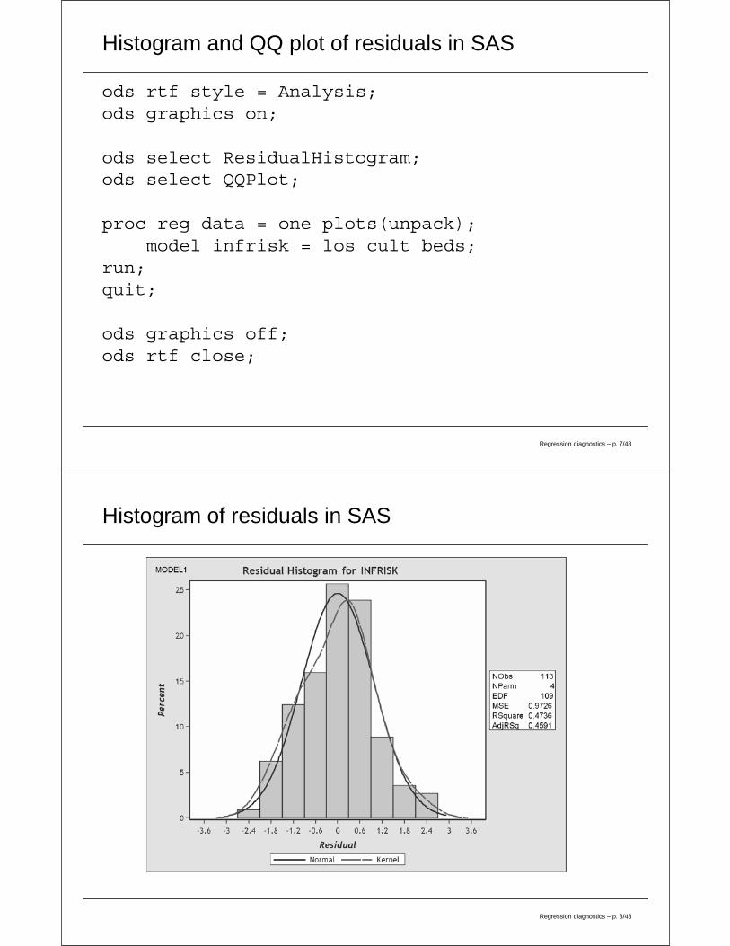
Recall that an assumption of linear regression is that the errorterms are normally distributed. That is ε ∼ Normal(0, σ2). Toassess this assumption, we will use the residuals to look at:
• histograms
• normal quantile-quantile (qq) plots
• Wilk-Shapiro test
Regression diagnostics – p. 6/48
Histogram and QQ plot of residuals in SAS
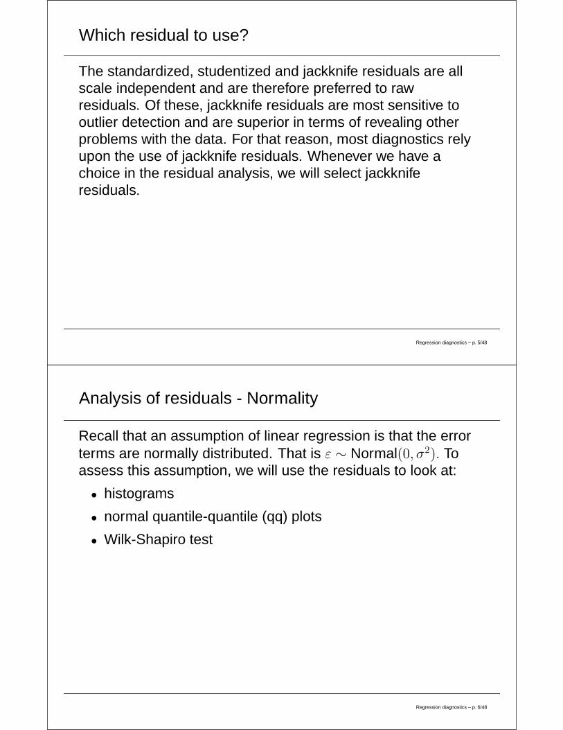
ods rtf style = Analysis;ods graphics on;
ods select ResidualHistogram;ods select QQPlot;
proc reg data = one plots(unpack);model infrisk = los cult beds;
run;quit;
ods graphics off;ods rtf close;
Regression diagnostics – p. 7/48
Histogram of residuals in SAS
Regression diagnostics – p. 8/48
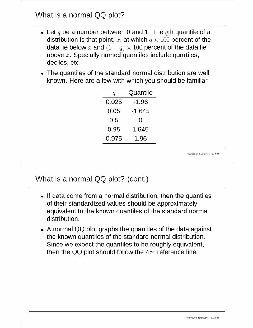
What is a normal QQ plot?
• Let q be a number between 0 and 1. The qth quantile of adistribution is that point, x, at which q × 100 percent of thedata lie below x and (1 − q) × 100 percent of the data lieabove x. Specially named quantiles include quartiles,deciles, etc.
• The quantiles of the standard normal distribution are wellknown. Here are a few with which you should be familiar.
q Quantile
0.025 -1.960.05 -1.6450.5 00.95 1.6450.975 1.96
Regression diagnostics – p. 9/48
What is a normal QQ plot? (cont.)
• If data come from a normal distribution, then the quantilesof their standardized values should be approximatelyequivalent to the known quantiles of the standard normaldistribution.
• A normal QQ plot graphs the quantiles of the data againstthe known quantiles of the standard normal distribution.Since we expect the quantiles to be roughly equivalent,then the QQ plot should follow the 45◦ reference line.
Regression diagnostics – p. 10/48
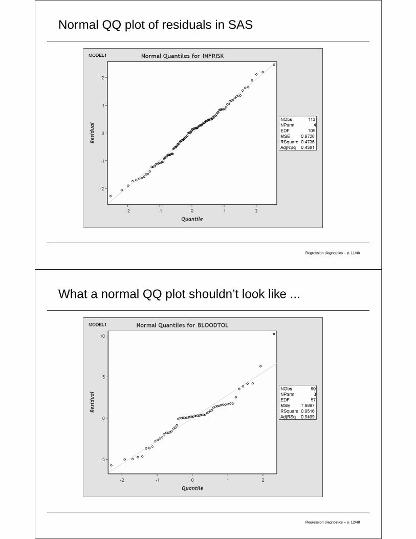
Normal QQ plot of residuals in SAS
Regression diagnostics – p. 11/48
What a normal QQ plot shouldn’t look like ...
Regression diagnostics – p. 12/48

The Wilk-Shapiro test
H0: The data are normally distributedHA: The data are not normally distributed
proc reg data = one noprint;model infrisk = los cult beds;output out = fitdata rstudent = jackknife;
run;quit;
proc univariate data = fitdata normal;var jackknife;
run;
Regression diagnostics – p. 13/48
The Wilk-Shapiro test (cont.)
Tests for Normality
Test -Statistic--- -----p Value------
Shapiro-Wilk 0.994445 Pr < W 0.9347
We fail to reject the null hypothesis and conclude that there isinsufficient evidence to conclude that the model errors are notnormally distributed.
Regression diagnostics – p. 14/48
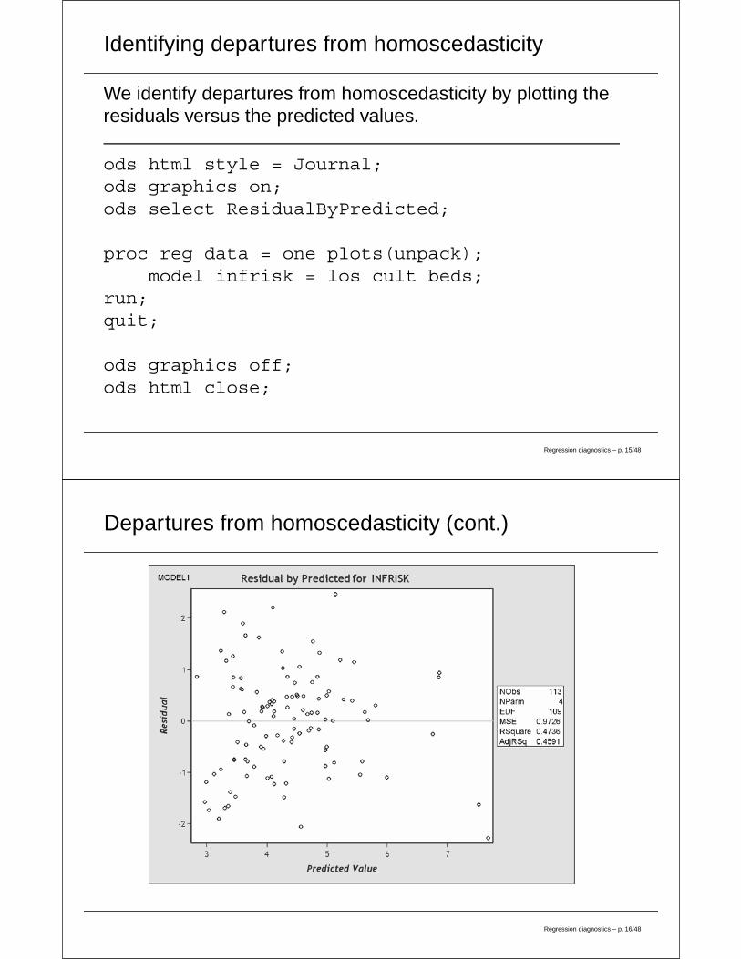
Identifying departures from homoscedasticity
We identify departures from homoscedasticity by plotting theresiduals versus the predicted values.
ods html style = Journal;ods graphics on;ods select ResidualByPredicted;
proc reg data = one plots(unpack);model infrisk = los cult beds;
run;quit;
ods graphics off;ods html close;
Regression diagnostics – p. 15/48
Departures from homoscedasticity (cont.)
Regression diagnostics – p. 16/48
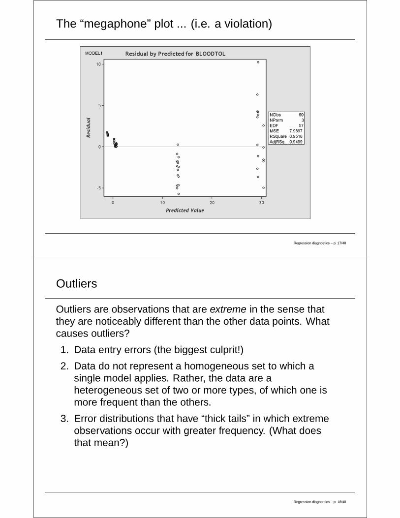
The “megaphone” plot ... (i.e. a violation)
Regression diagnostics – p. 17/48
Outliers
Outliers are observations that are extreme in the sense thatthey are noticeably different than the other data points. Whatcauses outliers?
1. Data entry errors (the biggest culprit!)
2. Data do not represent a homogeneous set to which asingle model applies. Rather, the data are aheterogeneous set of two or more types, of which one ismore frequent than the others.
3. Error distributions that have “thick tails” in which extremeobservations occur with greater frequency. (What doesthat mean?)
Regression diagnostics – p. 18/48

Outliers (cont.)
−6 −4 −2 0 2 4 6
0.0
0.1
0.2
0.3
0.4
Standard Normalt with 2 df
t dist has ’thicker tails’ than Normal
Regression diagnostics – p. 19/48
Outliers (cont.)
Sample from Normal (0,1) dist
Fre
quen
cy
−2 −1 0 1 2
05
1015
−2 −1 0 1 2
−2
01
2
Normal Q−Q Plot
Theoretical Quantiles
Sam
ple
Qua
ntile
s
Sample from t_2 df dist
Fre
quen
cy
−10 −5 0 5 10
010
30
−2 −1 0 1 2
−10
05
10
Normal Q−Q Plot
Theoretical Quantiles
Sam
ple
Qua
ntile
s
Regression diagnostics – p. 20/48
Outliers (cont.)
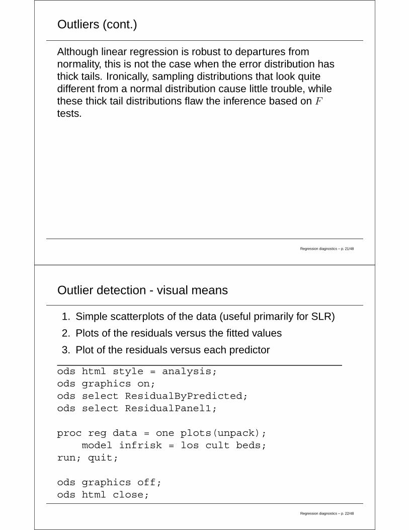
Although linear regression is robust to departures fromnormality, this is not the case when the error distribution hasthick tails. Ironically, sampling distributions that look quitedifferent from a normal distribution cause little trouble, whilethese thick tail distributions flaw the inference based on Ftests.
Regression diagnostics – p. 21/48
Outlier detection - visual means
1. Simple scatterplots of the data (useful primarily for SLR)
2. Plots of the residuals versus the fitted values
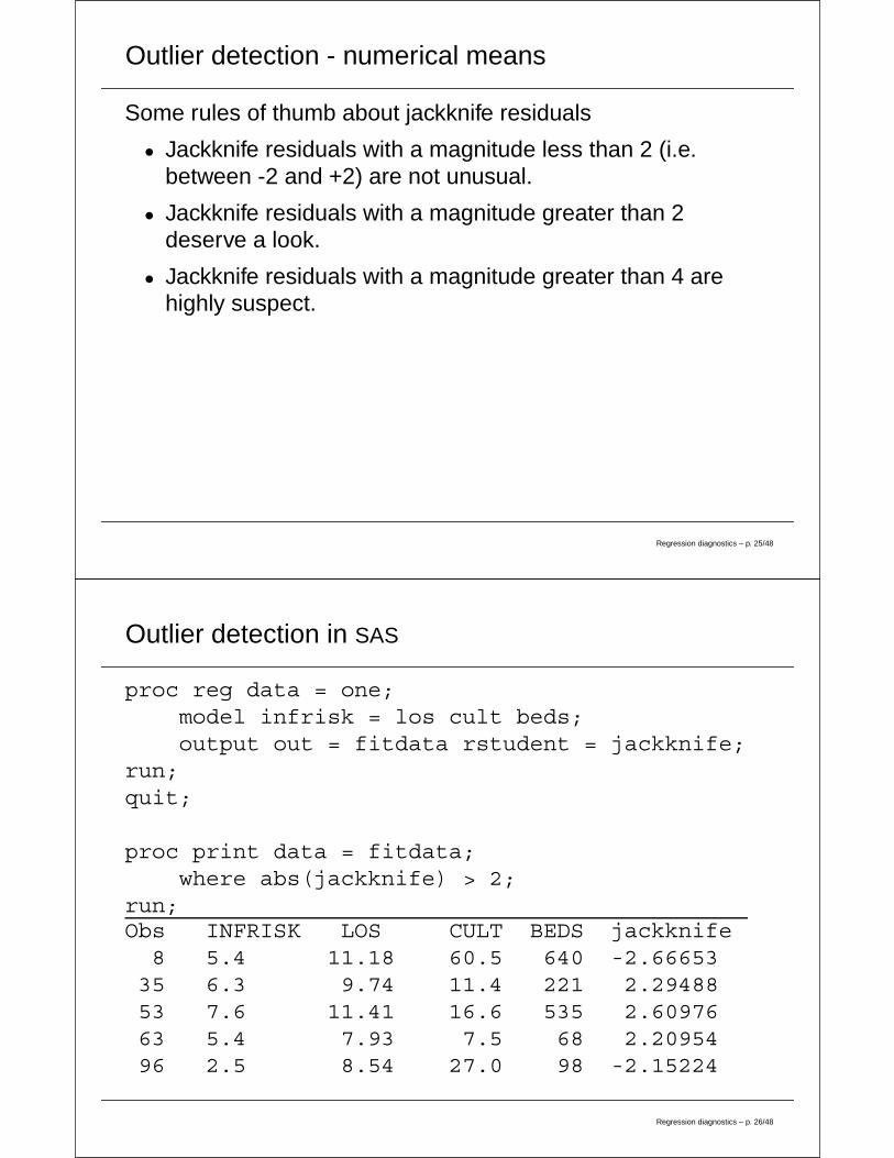
3. Plot of the residuals versus each predictor
ods html style = analysis;ods graphics on;ods select ResidualByPredicted;ods select ResidualPanel1;
proc reg data = one plots(unpack);model infrisk = los cult beds;
run; quit;
ods graphics off;ods html close;
Regression diagnostics – p. 22/48
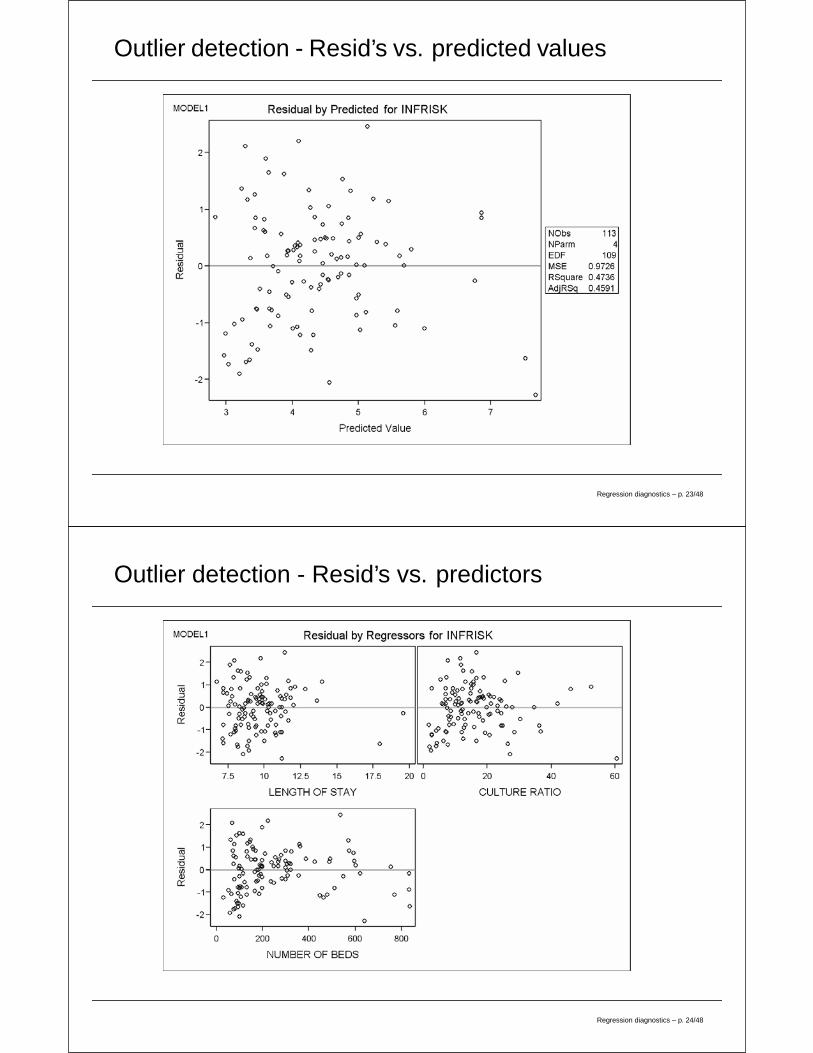
Outlier detection - Resid’s vs. predicted values
Regression diagnostics – p. 23/48
Outlier detection - Resid’s vs. predictors
Regression diagnostics – p. 24/48
Outlier detection - numerical means
Some rules of thumb about jackknife residuals
• Jackknife residuals with a magnitude less than 2 (i.e.between -2 and +2) are not unusual.
• Jackknife residuals with a magnitude greater than 2deserve a look.
• Jackknife residuals with a magnitude greater than 4 arehighly suspect.
Regression diagnostics – p. 25/48
Outlier detection in SAS
proc reg data = one;model infrisk = los cult beds;output out = fitdata rstudent = jackknife;
run;quit;
proc print data = fitdata;where abs(jackknife) > 2;
run;Obs INFRISK LOS CULT BEDS jackknife8 5.4 11.18 60.5 640 -2.6665335 6.3 9.74 11.4 221 2.2948853 7.6 11.41 16.6 535 2.6097663 5.4 7.93 7.5 68 2.2095496 2.5 8.54 27.0 98 -2.15224
Regression diagnostics – p. 26/48
Leverage and influence
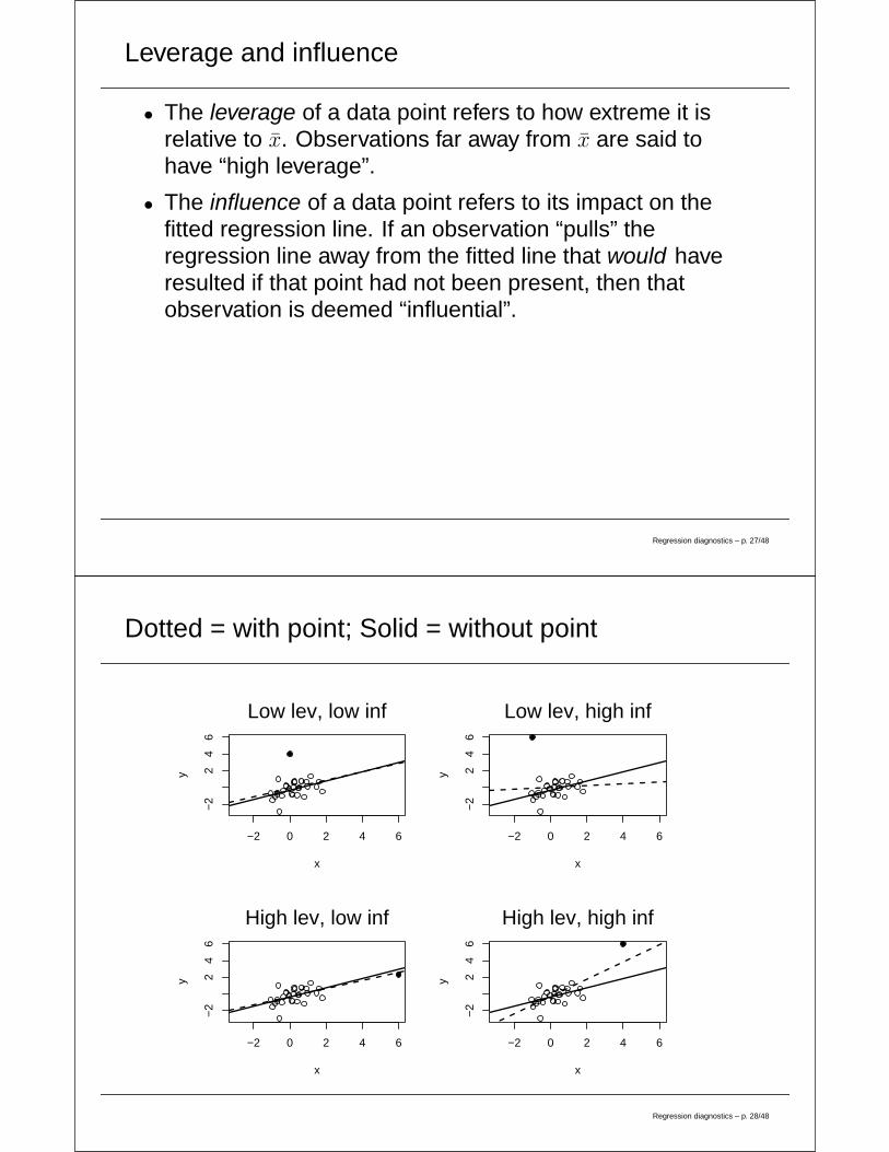
• The leverage of a data point refers to how extreme it isrelative to x. Observations far away from x are said tohave “high leverage”.
• The influence of a data point refers to its impact on thefitted regression line. If an observation “pulls” theregression line away from the fitted line that would haveresulted if that point had not been present, then thatobservation is deemed “influential”.
Regression diagnostics – p. 27/48
Dotted = with point; Solid = without point
−2 0 2 4 6
−2
24
6
x
y
Low lev, low inf
−2 0 2 4 6
−2
24
6
x
y
Low lev, high inf
−2 0 2 4 6
−2
24
6
x
y
High lev, low inf
−2 0 2 4 6
−2
24
6
x
y
High lev, high inf
Regression diagnostics – p. 28/48
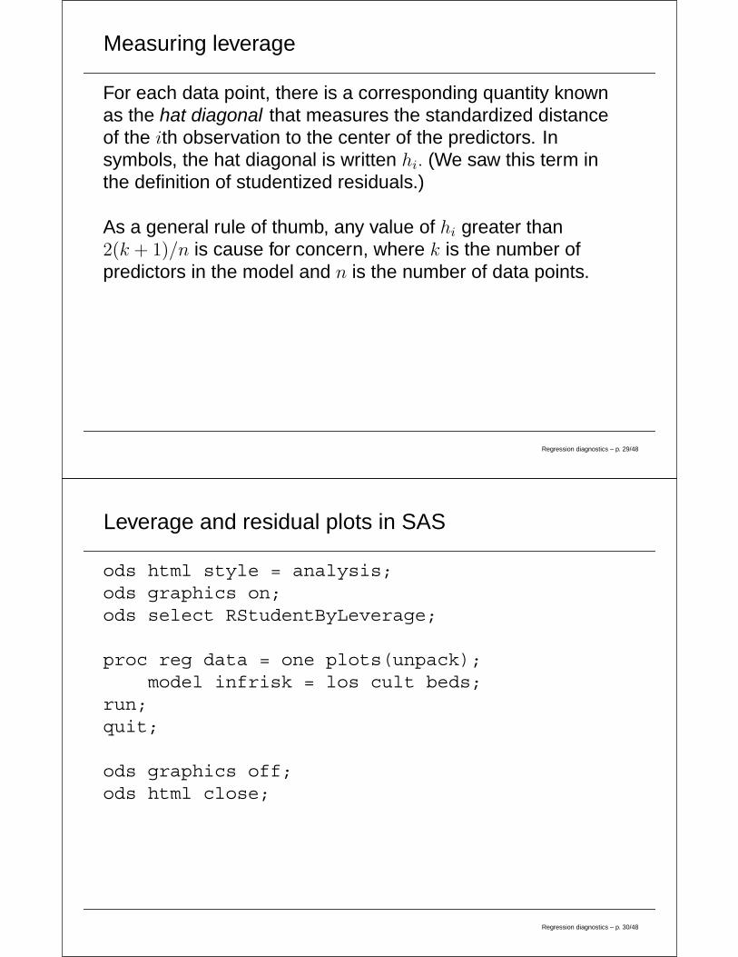
Measuring leverage
For each data point, there is a corresponding quantity knownas the hat diagonal that measures the standardized distanceof the ith observation to the center of the predictors. Insymbols, the hat diagonal is written hi. (We saw this term inthe definition of studentized residuals.)
As a general rule of thumb, any value of hi greater than2(k + 1)/n is cause for concern, where k is the number ofpredictors in the model and n is the number of data points.
Regression diagnostics – p. 29/48
Leverage and residual plots in SAS
ods html style = analysis;ods graphics on;ods select RStudentByLeverage;
proc reg data = one plots(unpack);model infrisk = los cult beds;
run;quit;
ods graphics off;ods html close;
Regression diagnostics – p. 30/48
Leverage and residual plots in SAS
Regression diagnostics – p. 31/48
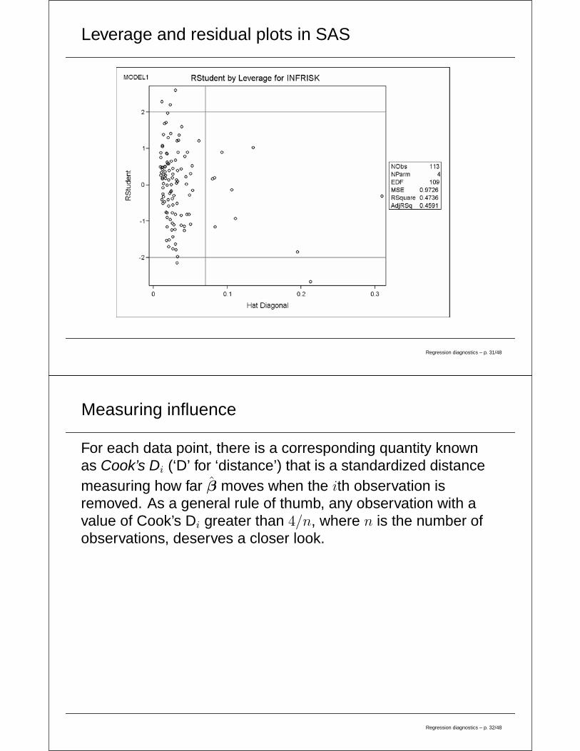
Measuring influence
For each data point, there is a corresponding quantity knownas Cook’s Di (‘D’ for ‘distance’) that is a standardized distancemeasuring how far β moves when the ith observation isremoved. As a general rule of thumb, any observation with avalue of Cook’s Di greater than 4/n, where n is the number ofobservations, deserves a closer look.
Regression diagnostics – p. 32/48
Graphing of Cooks D in SAS
ods html style = analysis;ods graphics on;ods select CooksD;
proc reg data = one plots(unpack);model infrisk = los cult beds;
run;quit;
ods graphics off;ods html close;
Regression diagnostics – p. 33/48
Graphing of Cooks D in SAS (cont.)
Regression diagnostics – p. 34/48
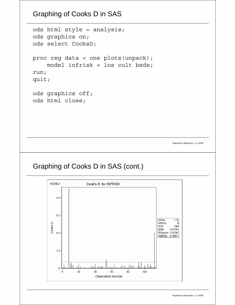
Leverage/influence - numerical assessment
proc reg data = one;model infrisk = los cult beds;output out = fitdata cookd = cooksd h = hat;
run;quit;
*(2*4)/113 = 0.071;proc print data = fitdata;
where hat ge (2*4)/113;run;
*4/113 = 0.035;proc print data = fitdata;
where cooksd ge 4/113;run;
Regression diagnostics – p. 35/48
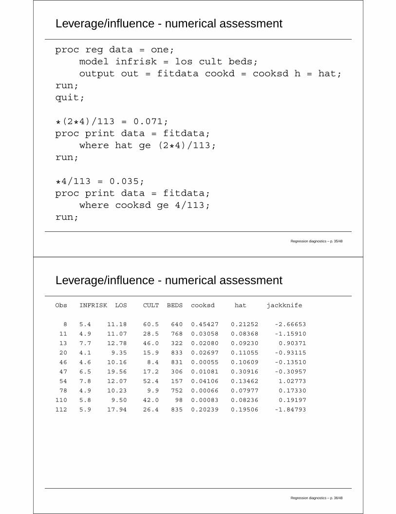
Leverage/influence - numerical assessment
Obs INFRISK LOS CULT BEDS cooksd hat jackknife
8 5.4 11.18 60.5 640 0.45427 0.21252 -2.66653
11 4.9 11.07 28.5 768 0.03058 0.08368 -1.15910
13 7.7 12.78 46.0 322 0.02080 0.09230 0.90371
20 4.1 9.35 15.9 833 0.02697 0.11055 -0.93115
46 4.6 10.16 8.4 831 0.00055 0.10609 -0.13510
47 6.5 19.56 17.2 306 0.01081 0.30916 -0.30957
54 7.8 12.07 52.4 157 0.04106 0.13462 1.02773
78 4.9 10.23 9.9 752 0.00066 0.07977 0.17330
110 5.8 9.50 42.0 98 0.00083 0.08236 0.19197
112 5.9 17.94 26.4 835 0.20239 0.19506 -1.84793
Regression diagnostics – p. 36/48

All the graphics in one panel
ods html style = analysis;ods graphics on;
proc reg data = one plots;model infrisk = los cult beds;
run;quit;
ods graphics off;ods html close;
Regression diagnostics – p. 37/48
All the graphics in one panel
Regression diagnostics – p. 38/48
Collinearity
Collinearity is a problem that exists when some (or all) of theindependent variables are strongly linearly associated withone another. If collinearity exists in your data, then thefollowing problems result.
• The estimated regression coefficients can be highlyinaccurate.
• The standard errors of the coefficients can be highlyinflated.
• The p-values, and all subsequent inference, can bewrong.
Regression diagnostics – p. 39/48
Symptoms of collinearity
• Large changes in coefficient estimates and/or in theirstandard errors when independent variables areadded/deleted.
• Large standard errors.
• Non-significant results for independent variables thatshould be significant.
• Wrong signs on slope estimates.
• Overall test significant, but partial tests insignificant.
• Strong correlations between independent variables.
• Large variance inflation factors (VIFs).
Regression diagnostics – p. 40/48

Variance inflation factor
For each independent variable Xj in a model, the varianceinflation factor is calculated as
VIFj =1
1 − R2
Xj∼all other Xs
where R2
Xj∼all other Xs is the usual R2 obtained by
regressing Xj on all the other Xs, and represents theproportion of variation in Xj that is explained by the remainingindependent variables. Therefore, 1 − R2
Xj∼all other Xs is a
measure of the variability in Xj that isn’t explained by theother independent variables.
Regression diagnostics – p. 41/48
Variance inflation factor (cont.)
When there is strong collinearity,
• R2
Xj∼all other Xs will be large
• 1 − R2
Xj∼all other Xs will be small, and so
• VIFj will be large.
As a general rule of thumb, strong collinearity is present whenVIFj > 10.
Regression diagnostics – p. 42/48
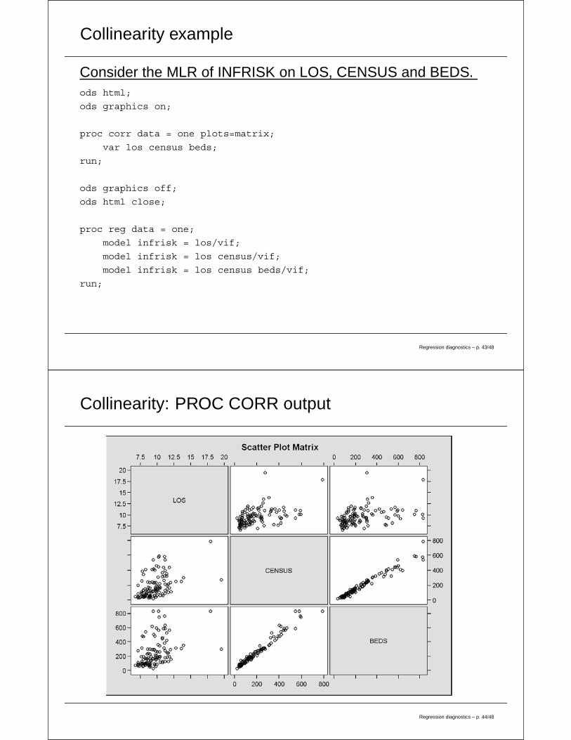
Collinearity example
Consider the MLR of INFRISK on LOS, CENSUS and BEDS.ods html;
ods graphics on;
proc corr data = one plots=matrix;
var los census beds;
run;
ods graphics off;
ods html close;
proc reg data = one;
model infrisk = los/vif;
model infrisk = los census/vif;
model infrisk = los census beds/vif;
run;
Regression diagnostics – p. 43/48
Collinearity: PROC CORR output
Regression diagnostics – p. 44/48
Collinearity: PROC CORR output (cont.)
Pearson Correlation Coefficients, N = 113
Prob > |r| under H0: Rho=0
LOS CENSUS BEDS
LOS 1.00000 0.47389 0.40927
LENGTH OF STAY <.0001 <.0001
CENSUS 0.47389 1.00000 0.98100
AVG DAILY CENSUS <.0001 <.0001
BEDS 0.40927 0.98100 1.00000
NUMBER OF BEDS <.0001 <.0001
Regression diagnostics – p. 45/48
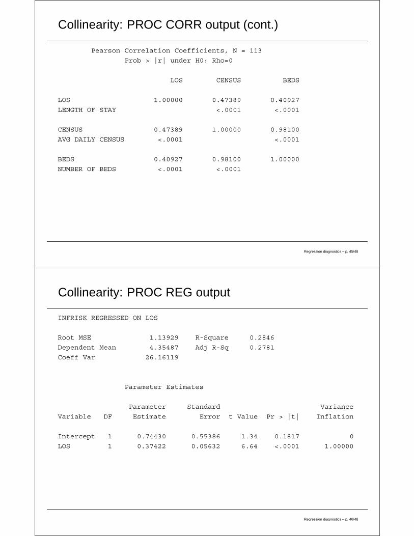
Collinearity: PROC REG output
INFRISK REGRESSED ON LOS
Root MSE 1.13929 R-Square 0.2846
Dependent Mean 4.35487 Adj R-Sq 0.2781
Coeff Var 26.16119
Parameter Estimates
Parameter Standard Variance
Variable DF Estimate Error t Value Pr > |t| Inflation
Intercept 1 0.74430 0.55386 1.34 0.1817 0
LOS 1 0.37422 0.05632 6.64 <.0001 1.00000
Regression diagnostics – p. 46/48

Collinearity: PROC REG output (cont.)
INFRISK REGRESSED ON LOS AND CENSUS
Root MSE 1.12726 R-Square 0.3059
Dependent Mean 4.35487 Adj R-Sq 0.2933
Coeff Var 25.88504
Parameter Estimates
Parameter Standard Variance
Variable DF Estimate Error t Value Pr > |t| Inflation
Intercept 1 0.99950 0.56531 1.77 0.0798 0
LOS 1 0.31908 0.06328 5.04 <.0001 1.28960
CENSUS 1 0.00145 0.00078668 1.84 0.0687 1.28960
Regression diagnostics – p. 47/48
Collinearity: PROC REG output (cont.)
INFRISK REGRESSED ON LOS, CENSUS AND BEDS
Root MSE 1.12953 R-Square 0.3094
Dependent Mean 4.35487 Adj R-Sq 0.2904
Coeff Var 25.93727
Parameter Estimates
Parameter Standard Variance
Variable DF Estimate Error t Value Pr > |t| Inflation
Intercept 1 0.82296 0.61382 1.34 0.1828 0
LOS 1 0.33538 0.06706 5.00 <.0001 1.44245
CENSUS 1 -0.00142 0.00392 -0.36 0.7177 31.90045
BEDS 1 0.00225 0.00302 0.75 0.4569 29.71362
Regression diagnostics – p. 48/48