Duisenberg school of finance - Tinbergen Institute Discussion Paper

TI 10-104 / DSF 2 Systemic Risk Diagnostics

Bernd Schwaab1

André Lucas2,3,4

Siem Jan Koopman2,3

1 European Central Bank, Financial Markets Research; 2 VU University Amsterdam; 3 Tinbergen Institute; 4 Duisenberg school of finance.

Tinbergen Institute is the graduate school and research institute in economics of Erasmus University Rotterdam, the University of Amsterdam and VU University Amsterdam. More TI discussion papers can be downloaded at http://www.tinbergen.nl Tinbergen Institute has two locations: Tinbergen Institute Amsterdam Roetersstraat 31 1018 WB Amsterdam The Netherlands Tel.: +31(0)20 551 3500 Fax: +31(0)20 551 3555 Tinbergen Institute Rotterdam Burg. Oudlaan 50 3062 PA Rotterdam The Netherlands Tel.: +31(0)10 408 8900 Fax: +31(0)10 408 9031

Duisenberg school of finance is a collaboration of the Dutch financial sector and universities, with the ambition to support innovative research and offer top quality academic education in core areas of finance.

More DSF research papers can be downloaded at: http://www.dsf.nl/ Duisenberg school of finance Roetersstraat 33 1018 WB Amsterdam Tel.: +31(0)20 525 8579

Systemic risk diagnostics∗

Bernd Schwaab,(a) Andre Lucas,(b,c) Siem Jan Koopman(b,d)

(a) European Central Bank, Financial Markets Research

(b) Tinbergen Institute

(c) Department of Finance, VU University Amsterdam

(d) Department of Econometrics, VU University Amsterdam

October 7, 2010

Abstract

A macro-prudential policy maker can manage risks to financial stability only if such

risks can be reliably assessed. To this purpose we propose a novel framework for

systemic risk diagnostics based on state space methods. We assess systemic risk based

on latent macro-financial and credit risk components in the U.S., the EU-27 area, and

the rest of the world. The time-varying probability of a systemic event, defined as the

simultaneous failure of a large number of bank and non-bank intermediaries, can be

assessed in- and out of sample. Credit and macro-financial conditions are combined

into a straightforward coincident indicator of system risk. In an empirical analysis

of worldwide default data, we find that credit risk conditions can significantly and

persistently decouple from business cycle conditions due to e.g. unobserved changes in

credit supply. Such decoupling is an early warning signal for macro-prudential policy.

Keywords: financial crisis; systemic risk; credit portfolio models; frailty-correlated

defaults; state space methods.

JEL classification: G21, C33

∗Corresponding author: Bernd Schwaab, European Central Bank, Kaiserstrasse 29, 60311 Frankfurt,Germany. Tel. +49 69 1344 7216. Email: Bernd.Schwaab@ecb.int. We thank Christian Brownlees, PhilippHartmann, Robert Engle, and Michel van der Wel for comments. This research was written while Schwaabwas at the Finance Department of VU University Amsterdam and Tinbergen Institute. The views expressedin this paper are those of the authors and they do not necessarily reflect the views or policies of the EuropeanCentral Bank or the European System of Central Banks.

1

”One of the greatest challenges ... at this time is to restore financial and economic stability. ...

The academic research community can make a significant contribution in supporting policy-makers

to meet these challenges. It can help to improve analytical frameworks for the early identification

and assessment of systemic risks.” Jean-Claude Trichet, President of the ECB, Clare Distinguished

Lecture in Economics and Public Policy, University of Cambridge, December 2009.

”We have enough agreement on the broad principles of financial regulations, and we need to get

down to specifics. I would therefore consider any future report that does not include tables, figures,

numbers, equations, and specific proposals to be useless rhetoric.” Thomas Philippon, ”An overview

of the proposals to fix the financial system”, Feb 2009, commentary on VoxEU.org.

1 Introduction

The debate on macro-prudential policies ignited by the recent financial crisis is currently

under full swing. Various commentators agree that policy makers have heretofore overlooked

important aspects of the macro-financial economic environment. For example, regulators

have learned the hard way that asset and credit exposures that are safe on the micro level

can have severe consequences if they are highly correlated (of high systematic risk) in the

cross section. Such dependence undermines positive effects from diversification at the firm

level, and may further lead to a ‘fallacy of composition’ at the systemic level, as described

e.g. in Brunnermeier, Crocket, Goodhart, Persaud, and Shin (2009). Essentially, traditional

risk-based capital regulation alone may underestimate systemic risk by neglecting the macro

impact of banks reacting in unison to a shock.

Macro-prudential oversight seeks to focus on the financial system as a whole. It has been

assigned to new regulatory councils, such as the European Systemic Risk Board (ESRB) in

the European Union, and the Financial Stability Oversight Council (FSOC) in the United

States. Each board has a mandate to identify, assess, and prioritize system-wide risks, and

to formulate recommendations to mitigate them. There is widespread agreement that finan-

cial systemic risk is characterized by both cross-sectional and time-related dimensions, see

e.g. Hartmann, de Bandt, and Alcalde (2009). The cross sectional dimension concerns how

risks are correlated across financial institutions at a given point in time (due to e.g. conta-

gion across institutions, and prevailing default conditions at that time), while the time-series

dimension concerns how systemic risk evolves over time (e.g. due to changes in the default

cycle, changes in financial market conditions, and the potential buildup of financial imbal-

ances).

While there is broad consensus on the set of models, indicators, and analytical tools for

1

e.g. macroeconomic and monetary policy analysis, such agreement is yet absent for macro-

prudential policy analysis. This paper seeks to help fill this important gap. In particular,

we make three contributions to the literature on systemic risk assessment.

First, we propose a novel econometric framework for the measurement of global macro-

financial and credit risk conditions based on state space methods. Essentially, the model is a

high-dimensional diagnostic tool that tracks the evolution of macro-financial developments

and point in time risk conditions, and their joint impact on system stability. It is clear that

what can’t be measured can’t be managed. As a result, a reliable and accurate diagnostic

tool for systemic risk assessment is desperately needed.

Among other issues when modeling credit market developments, commentators of the re-

cent financial crisis stress the importance of an international perspective, see e.g. de Larosiere

(2009), and Brunnermeier et al. (2009). This requires looking beyond domestic developments

to detect risks to financial stability. For the recent crisis, the saving behavior of Asian coun-

tries has been cited as a contributing factor to low interest rates and easy credit access in

the U.S., see e.g. Brunnermeier (2009). Similarly, it is the exposure to developments in

the U.S. housing market that triggered financial distress for European financial institutions.

We therefore consider three broad geographical regions, i.e., (i) the U.S., (ii) current EU-27

countries, and (iii) all remaining countries. The large-dimensional latent factor model allows

for the differential impact of world business cycle conditions on regional default rates, latent

regional risk factors, as well as world-wide industry sector/contagion dynamics.

As the paper’s second main contribution, we present a coincident indicator for unobserved

default stress. When applied to financial firms, the indicator is a straightforward measure

for overall financial system risk. Making use of a narrower definition, the underlying time-

varying probability of a systemic event, defined as the simultaneous failure of a large number

of bank and non-bank intermediaries, can also be assessed and forecast out-of-sample.

Default clustering is the main risk in the banking book, and therefore central to financial

stability assessment. However, the accurate measurement of point-in-time credit risk condi-

tions is complicated since not all processes that determine corporate and financial distress

are easily observed. Recent research indicates that readily available macro-financial vari-

ables and firm-level information may not be sufficient to capture the large degree of default

clustering present in corporate default data. In an important study for U.S. data, Das,

Duffie, Kapadia, and Saita (2007) reject the joint hypothesis of well-specified default inten-

sities in terms of (a) observed macroeconomic variables and firm-specific risk factors and (b)

the conditional independence (doubly stochastic default times) assumption. In particular,

there is substantial evidence for an additional dynamic unobserved ‘frailty’ risk factor as

2

well as contagion dynamics, see McNeil and Wendin (2007), Das et al. (2007) Azizpour and

Giesecke (2008), Koopman, Lucas, and Monteiro (2008), Koopman and Lucas (2008), Lando

and Nielsen (2008), and Duffie, Eckner, Horel, and Saita (2009). ‘Frailty’ and contagion risk

causes default dependence above and beyond what is implied by observed covariates alone.

For U.S. data, Koopman, Lucas, and Schwaab (2010) find that frailty effects account for

30–60% of systematic default rate variation. Based on these results, our model is set up to

explicitly accommodate latent dynamic components.

In an empirical analysis of worldwide credit data for more than 12.000 firms, we sug-

gest that the magnitude of such frailty effects (autonomous default dynamics) can serve as a

warning signal for macro-prudential policy makers. Frailty effects are highest when aggregate

default conditions (the ‘default cycle’) diverge significantly from aggregate macroeconomic

conditions (the ‘business cycle’), e.g. due to unobserved shifts in credit supply. Historically,

frailty effects have been pronounced during bad times, such as the savings and loan crisis

in the U.S. leading up to the 1991 recession, or exceptionally good times, such as the years

2005-07 leading up to the recent financial crisis. In the latter years, default conditions are

much more benign than would be expected from observed macro and financial data. In either

case, a macro-prudential policy maker should be aware of a possible decoupling of system-

atic default risk conditions from where they should be based on observed macro-financial

conditions. In this regard, the monitoring of both business and credit cycle conditions is key.

1.1 New quantitative measures of systemic risk: the post-crisis

literature

A host of new quantitative measures of systemic risk have recently been proposed in the

academic and central banking literature. This section briefly surveys these measures and

frameworks. We understand systemic risk as the risk that financial instability becomes so

widespread that it impairs the functioning of a financial system to the point where economic

growth and welfare suffer materially, see ECB (2009). This notion is made operational as

the risk of experiencing a systemic event. The nature of the systemic event may then depend

on the adopted modeling framework.

Systemic risk is a complex and diffuse concept. It may therefore be helpful to distinguish

between different sources of system risk, see e.g. ECB (2009) and Trichet (2009). First,

financial system contagion risk refers to an initially idiosyncratic problem that becomes more

widespread in the cross section, often in a sequential fashion. Second, shared exposure to

financial market shocks and macroeconomic developments may cause simultaneous problems

for financial intermediaries. Third, financial imbalances such as credit and asset market

3

bubbles that build up gradually over time may unravel suddenly, with detrimental effects on

the system. We review the literature based on this distinction.

Financial market shock: Acharya, Pedersen, Philippon, and Richardson (2010) show

how each financial institution’s contribution to overall systemic risk can be measured. The

extent to which an institution imposes a negative externality on the system is called sys-

temic expected shortfall (SES), and can be estimated and aggregated. An institution’s SES

increases in its leverage and MES, marginal expected shortfall. Brownlees and Engle (2010)

use advanced econometric techniques to estimate MES. Huang, Zhou, and Zhu (2009, 2010)

propose a systemic risk measure called the distress insurance premium, or DIP, which rep-

resents a hypothetical insurance premium against systemic financial distress. Adrian and

Brunnermeier (2009) suggest CoVaR, the Value at Risk of the financial system conditional

on an individual institution being under stress. These methods are targeted more towards

the identification of systemically important institutions rather than an assessment of overall

system risk. They are also based squarely on changes in equity prices.

Contagion/Cross-sectional perspective: Contagion risk refers to an initially idiosyn-

cratic problem that becomes more widespread in the cross-section. Segoviano and Goodhart

(2009) define banking stability measures based on a non-parametric copula approach. Billo,

Getmansky, Lo, and Pelizzon (2010) capture dependence between intermediaries through

principal components analysis and predictive causality tests. Similarly, Hartmann, Straet-

mans, and de Vries (2005) derive indicators of the severity of banking system risk from

asymptotic interdependencies between banks’ equity prices based on multivariate extreme

value theory. This literature recognizes system risk as largely resulting from multivariate

(tail) dependence.

Macroeconomic shock: Macroeconomic shocks matter for financial stability because

they tend to affect all firms in an economy. A macro shock causes an increase in correlated

default losses, with detrimental effects on intermediaries’ profits and thus financial stability.

Aikman et al. (2009) propose a ‘Risk Assessment Model for Systemic Institutions’ (RAMSI)

to assess the impact of macroeconomic and financial shocks on both individual banks as

well as the banking system. Giesecke and Kim (2010) define systemic risk as the conditional

(time-varying) probability of failure of a large number of financial institutions, based on a

dynamic hazard rate model. A similar study based on a large number of macroeconomic

and financial covariates is Koopman, Lucas, and Schwaab (2008).

Financial imbalances: Financial imbalances such as credit and asset market bubbles

may build up gradually over time, but may also unravel suddenly with detrimental effects on

intermediaries and markets. Financial imbalances are not easily characterized and difficult

4

to quantify. Inference on financial misalignments can be based on observed covariates, such

as private credit-to-GDP ratio, total lending growth, changes in property and asset prices,

etc., see e.g. Borio and Lowe (2002), Misina and Tkacz (2008), and Barrell, Davis, Karim,

and Liadze (2010). Despite recent progress, these models still leave large errors in the ability

to predict financial stress.

We conclude the following. There is currently no widely accepted indicator or quantitative

framework that measures either banking or financial stability with sufficient accuracy and

breadth. Although notable progress has recently been achieved, even the most sophisticated

tools so far only account for a certain ’form’ of systemic risk, and often rely on narrow

definitions of a systemic event. The development of a broader and deeper yet still tractable

quantitative framework is the purpose of this paper.

1.2 What is needed?

In this section we identify four core features that - in our opinion - a ‘good’ diagnostic

framework for systemic risk should have. We will refer to this listing when introducing the

features of our econometric framework below.

First, even the most sophisticated tools so far rely on narrow definitions of a systemic

event. For example, Acharya et al. (2010) and Brownlees and Engle (2010) define a systemic

event as a large decline in equity prices. A more comprehensive framework could be based

on e.g. theoretical work by Goodhart, Sunirand, and Tsomocos (2006). Here, systemic

risk arises from (i) contagion dynamics at the financial industry level, (ii) shocks to the

macroeconomic and financial markets environment, and (iii, often implicitly) the potential

unraveling of imbalances. These sources of systemic risk act on observed data simultaneously.

For example, contagion is a more acute concern in a business cycle downturn, when confidence

and cash flows abate. Similarly, even a small financial market shock may prick a sufficiently

pent-up financial imbalance. Consequently, these forms of unobserved risks should all - in

one way or another - be part of a diagnostic framework. This is important. For example,

allowing for contagion through links but not for common factors may attribute observed

dependence to ‘links’ that do not exist.

Second, commentators of the recent financial crisis stress the importance of an interna-

tional perspective, see e.g. Brunnermeier et al. (2009), de Larosiere (2009) and Volcker et al.

(2009). Before the recent crisis, the saving behavior of Asian countries contributed to low

interest rates and easy credit access in the U.S. Similarly, it is the exposure to developments

in the U.S. housing market that triggered financial distress for European financials. Con-

sequently, a macro-prudential policy maker needs to look beyond domestic developments to

5

detect risks to financial stability. Diagnostic tools should reflect this key lesson from the fi-

nancial crisis. Given globalized financial markets, an exclusive focus on domestic conditions

is an exercise in self-deception.

Third, default clustering is the main source of risk in the banking book. Adverse changes

in macro-financial conditions affect the solvency of all firms in an economy, financial and

non-financial. Observed macro-financial risk factors are therefore systematic and correlate

defaults in the cross section. These default clusters have a first order impact on interme-

diaries’ profitability and solvability, and therefore on financial stability. In our opinion,

macro-financial and credit risk conditions, and little else, should be at the core of systemic

risk assessment.

Fourth, financial institutions rarely default. This is particularly the case in Europe,

where we count 12 financial defaults from 1981Q1 to 2010Q1. Data scarcity creates obvious

problems in the modeling of shared financial distress and financial default dependence. As a

result, models based on actual default experience only may give a partial picture of current

stress. Other measures of credit risk should therefore complement historical information.

One candidate are expected default frequencies (EDF) from structural models of credit risk

based on forward-looking stock market data and balance sheet information.

Section 2 below introduces a modeling framework based on state space methods that

combines these desired features into a tractable framework.

1.3 Why state space methods?

Systemic risk, and the conditional probability of a systemic event, regardless of the adopted

definition, are unobserved and time-varying quantities. Attributing overall system risk to

underlying constituents such as contagion risk at the financial sector level, changes in shared

and therefore systematic macro-financial conditions, and financial imbalances such as a lend-

ing bubble, as in ECB (2009, 2010), does not help immediately for systemic risk assessment,

since these three sources of risk are again time varying and unobserved. Latent and time-

varying states of interest are known to econometricians as unobserved components. It is

therefore natural to use unobserved component techniques to back out the location of latent

risk factors related to system risk from observed data.

2 The diagnostic framework

This section introduces the simplest possible econometric model that captures the desired

features from Section 1.2. The main idea is to infer unobserved sources of system risk from

6

panels of observed data. Once these latent factors are estimated, they can be combined into

a measure of system risk.

Credit risk is the main risk in the banking book. As a result, credit conditions are central

to systemic risk assessment. We consider macroeconomic and financial market covariates xt,

count data based on historical default experience yt, and expected default frequencies (EDFs)

zt denoted by

xt = (x1t, . . . , xNt)′ (1)

yt = (y1,1t, . . . , y1,Jt, . . . , yR,1t, . . . , yR,Jt)′ (2)

zt = (z1,1t, . . . , z1,St, . . . , zR,1t, . . . , zR,St)′ (3)

for t = 1, . . . , T , where yr,t and zr,t are default counts and EDF data, respectively, for firms

from a given economic region r = 1, . . . , R and cross section j = 1, . . . , J . We assume that

all data xt, yt, and zt are driven by dynamic factors.

The model combines normally and non-normally distributed observations. Conditional

on latent factors ft, the measurements are independent. In our specific case, we assume

that elements of xt conditional on ft follow a normal distribution with time-varying mean.

Further, conditional on ft, default counts yr,jt are binomially distributed with kr,jt trials and

time-varying probability πr,jt. Here, kr,jt denotes the number of firms in a specific ratings

and industry bucket j in region r at time t, while πr,jt is the time-varying probability of

default. The expected default frequencies zt are transformed to a quarterly horizon, and

to a log-odds ratio as zt = log (zt/(1− zt)). The log-odds are modeled as conditionally

Gaussian. The factor structure distinguishes macro, frailty, industry-specific (contagion)

effects, denoted fmt , fd

t , f it , respectively. These latent factors are the main input for our

systemic risk measure.

xnt|fmt ∼ Gaussian

(µnt, σ

2n

), (4)

yr,jt|fmt , fd

t , f it ∼ Binomial (kr,jt, πr,jt) (5)

zr,st|fmt , fd

t , f it ∼ Gaussian

(µst, σ

2s

). (6)

Factors fmt capture shared business cycle dynamics in both macro and credit risk data, and

are therefore common to xt, yt, and zt. The frailty factors fdt are region-specific, i.e., they

only load on realized defaults yr,t and (log-odds of) expected default rates zr,t from region

r. The frailty factors and independent of observed macroeconomic and financial data, and

7

thus pick up any default risk-specific variation above and beyond that is implied by macro

factors fmt . Latent factors f i

t affects firms in the same industry. Such factors may arise as a

result of default contagion through up- and downstream business links. Alternatively, they

may capture the industry-specific propagation of macro and financial shocks.

The point-in-time default probabilities πr,jt in (5) can also be referred to as (discrete

time) hazard rates, or default intensities. They vary over time due to shared exposure to

observed risk factors xt as summarized by fmt , frailty effects fd

t , and latent industry specific

effects f it . We model πr,jt as the logistic transform of an index function θr,jt,

πr,jt =(1 + e−θr,jt

)−1, (7)

where θr,jt may be interpreted as the log-odds or logit transform of πr,jt. This transform

yields convenient expressions and ensures that conditional probabilities πr,jt are in the unit

interval.

The panel data dynamics in observed data (1) to (3) are captured by time-varying pa-

rameters, or ‘signals’, given by

µnt = cn + β′nfmt , (8)

θr,jt = λr,j + β′r,jfmt + γ′r,jf

dt + δ′r,jf

it , (9)

µr,st = cr,s + β′r,sfmt + γ′r,sf

dt + δ′r,sf

it , (10)

where λr,j, cn, and cr,s are fixed effects, and risk factor sensitivities β, γ, and δ refer to macro

factors, frailty factors, and industry-specific factors, respectively. Fixed effects and factor

loadings may differ across firms and regions. Since the cross-section is high-dimensional, we

follow Koopman and Lucas (2008) in reducing the number of parameters by imposing the

following additive structure

χr,j = χ0 + χ1,dj+ χ2,sj

+ χ3,rj, χ = λ, β, γ, δ, β, γ, δ (11)

where χ0 represents the baseline effect, χ1,d is the industry-specific deviation, χ2,s is the

deviation related to rating group, χ3,r is the deviation related to economic region. Due to

the common effect χ0, some specific coefficients need to be set to zero for model identification.

This parameter specification combines model parsimony with a sufficiently large degree of

flexibility to fit the data.

All latent factors are stacked into the vector ft =(fm′

t , fd′t , f i′

t

)′, and follow simple au-

8

toregressive dynamics,

ft = Φft−1 + ηt, ηt ∼ NID (0, Ση) (12)

where the coefficient matrix Φ is diagonal, and Ση is a covariance matrix of full rank. The

autoregressive structure allows the components of ft to be sticky. For example, it allows the

macroeconomic factors fmt to evolve slowly over time and capture business cycle dynamics

in macro and default data. Similarly, the credit climate and industry default conditions are

captured by persistent processes for fdt and f i

t , such that they can capture the clustering

of high-default years. The initial condition f1 ∼ N(0, Σ0) completes the specification of the

factor process. The m×1 disturbance vectors ηt are serially uncorrelated. For identification,

we require Ση = I − ΦΦ′. This implies E[ft] = 0, Var[ft] = I, and Cov[ft, ft−h] = Φh for

h = 1, 2, ... It identifies loading coefficients βr,j, γr,j, and δr,j in (9) as risk factor volatilities

(standard deviations) for firms in cross section (r, j).

2.1 Parameter and factor estimation

Equations (1) to (12) form a mixed measurement dynamic factor model (MM-DFM) as

described in Koopman, Lucas, and Schwaab (2010) and Creal, Schwaab, Koopman, and

Lucas (2010). Unfortunately, the log-likelihood does not exist in closed form for this class

of models, due to the presence of non-Gaussian data in yt and autocorrelated unobserved

factors ft. We overcome this issue by casting the model (1) to (12) to state space form,

and then estimating parameters and latent factors using Monte Carlo maximum likelihood

methods based on importance sampling. We refer to the Appendix A1 for estimation details.

Missing values may be ubiquitous in the panel (1) to (3). For example, certain covariates

in xt may not be available at the beginning of the sample. Also, default data yr,jt is missing

if there are no corresponding firms at risk in cell kr,jt. Similarly, data on implied expected

default frequencies may be unavailable at the beginning of the sample. Missing values can

be taken into account in our mixed measurement framework as outlined in the Appendix

A2.

The cross sectional dimension of the data (1) to (3) may easily become large. Potentially

many parameters and latent factors need to be estimated by numerically maximizing the log-

likelihood function over a large dimensional space. A technique to increase computational

speed is required, and can be based on a recent result by Jungbacker and Koopman (2008).

Appendix A3 extends their method of collapsing observations into a subspace to the case of

a nonlinear mixed measurement factor model.

9

2.2 Systematic default risk indicator

We now present the indicator for common default stress. For example, we are interested in

the level of common stress for U.S. and European financial firms. The indicator is based on

the above modeling framework. As a result, it summarizes the macro, frailty, and contagion

effects driving default into a single metric.

Default signals θr,jt in (9) capture the level and time variation in the log-odds of condi-

tional default probabilities πr,jt over time for firms in region r and cross section j. Signals

θr,jt consist of two terms,

θr,jt = [λr,j] +[β′r,jf

mt + γ′r,jf

dt + δ′r,jf

it

],

where, fixed effects λr,j pin down the through-the-cycle default rate, while systematic factors

fmt , fd

t , and f it jointly determine the point-in-time default conditions. The aggregation of

signals θr,jt over cross sections j can be achieved by pooling the factor loadings for these

firms. Where this is not appropriate, one may use the fact that default intensities πr,jt are

additive, see Lando (2003, Chapter 5).

Signals θr,jt are Gaussian since all risk factors in ft are Gaussian. Standardized signals

zθr,jt are unconditionally standard normal, and obtained as

zθr,jt = (θr,jt − λr,j) /

√Var(θr,jt),

where Var(θr,jt) = β′r,jβr,j + γ′r,jγr,j + δ′r,jδr,j ≥ 0 is the unconditional variance of θr,jt. Our

systematic credit risk indicator (SRI) for firms of type j in region r at time t is given by

SRIr,jt = 100Φ(zθ

r,jt

), (13)

where Φ(z) is the standard normal cumulative distribution function. Values of SRIr,jt lie

between 0 and 100 by construction with uniform (unconditional) probability. Values below

50 indicate less-than-average common default stress, while values above 50 suggest above-

average stress. Values below 25, say, are exceptionally benign, and values above 75 are

indicative of substantial systematic stress. Our measure of financial system risk is obtained

when (13) is applied to model-implied hazards rates for financial firms in a given region.

10

3 Data

We use data from two main sources in the empirical study below. First, a panel of macroe-

conomic and financial time series data is taken from Datastream with the aim to capture

international business cycle and financial market conditions. Macroeconomic data is ob-

tained for different economic regions, including the U.S. and the EU-27 countries. Table 1

provides a listing. The macro variables enter the analysis as annual growth rates from

1980Q1 to 2009Q4.

A second dataset is constructed from default data from Moody’s. The database contains

rating transition histories and default dates for all rated firms (worldwide) from 1980Q1

to 2009Q4. This data allows to determine quarterly values for yr,jt and kr,jt in (5). The

database distinguishes 12 industry sectors which we pool into seven industry groups, see the

first column of Table 2 for a listing. We consider four broad rating groups, investment grade

Aaa−Baa, and three speculative grade groups Ba, B, and Caa−C. For details on default

and exposure data we refer to the Appendix A4.

Table 2 provides an overview of the international exposure and default count data. Cor-

porate data is most numerous for the U.S., with E.U. countries second. Most firms are either

from the industrial or financial sector. The bottom of Table 2 suggests that about 60% of

all worldwide ratings are investment grade. European and Asian firms are more likely to be

rated investment grade, with shares of 83% and 75%, respectively. Table 3 lists the countries

contained in each region, along with the respective number of defaults and firms. Figure 1

plots aggregate default counts, exposures, and observed fractions over time for each of the

four regions.

11

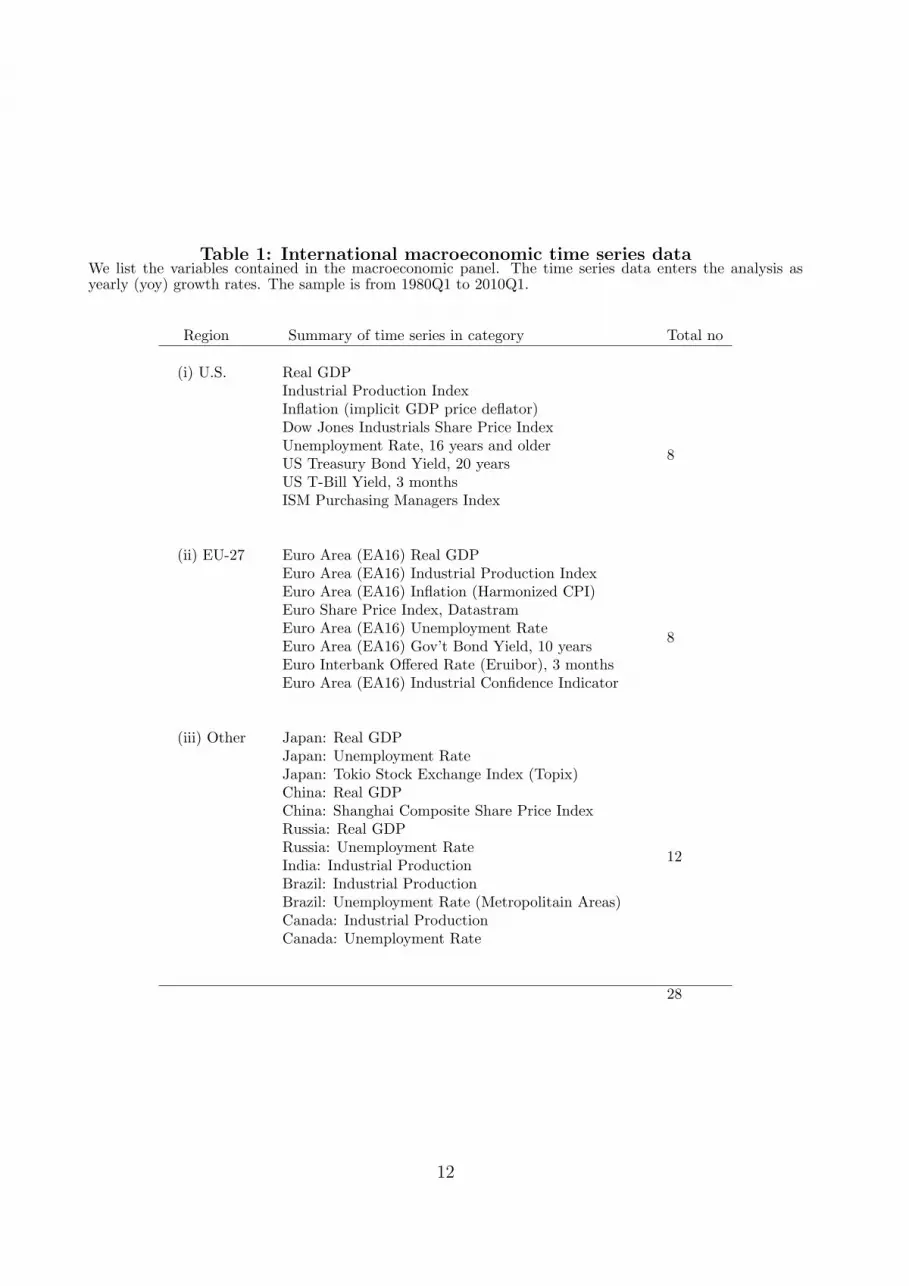
Table 1: International macroeconomic time series dataWe list the variables contained in the macroeconomic panel. The time series data enters the analysis asyearly (yoy) growth rates. The sample is from 1980Q1 to 2010Q1.

Region Summary of time series in category Total no

(i) U.S. Real GDPIndustrial Production IndexInflation (implicit GDP price deflator)Dow Jones Industrials Share Price IndexUnemployment Rate, 16 years and olderUS Treasury Bond Yield, 20 yearsUS T-Bill Yield, 3 monthsISM Purchasing Managers Index

8

(ii) EU-27 Euro Area (EA16) Real GDPEuro Area (EA16) Industrial Production IndexEuro Area (EA16) Inflation (Harmonized CPI)Euro Share Price Index, DatastramEuro Area (EA16) Unemployment RateEuro Area (EA16) Gov’t Bond Yield, 10 yearsEuro Interbank Offered Rate (Eruibor), 3 monthsEuro Area (EA16) Industrial Confidence Indicator

8

(iii) Other Japan: Real GDPJapan: Unemployment RateJapan: Tokio Stock Exchange Index (Topix)China: Real GDPChina: Shanghai Composite Share Price IndexRussia: Real GDPRussia: Unemployment RateIndia: Industrial ProductionBrazil: Industrial ProductionBrazil: Unemployment Rate (Metropolitain Areas)Canada: Industrial ProductionCanada: Unemployment Rate

12

28

12

Table 2: International default and exposure countsThe top panel presents default counts disaggregated across industry sectors and economic region. The‘Other’ column is disaggregated into Asian and remaining countries and corresponds to Table 3. The middlepanel presents the total number of firms counted from 1981Q1 to 2010Q1. The bottom panel presents thecross section of firms at risk (‘exposures’) at point-in-time 2008Q1 according to rating group and economicregion.

Defaults U.S. Europe Asia Remainder SumBank 41 8 9 13 71Fin non-Bank 84 4 8 6 102Transport 90 17 1 7 115Media 127 2 0 2 131Leisure 97 9 1 14 121Utilities 24 2 0 5 31Energy 79 0 1 6 86Industrial 435 16 16 37 504Technology 177 38 3 21 239Retail 94 1 2 2 99Cons Goods 120 8 3 14 145Misc 31 0 4 12 47Sum 1399 105 48 139 1691

Firms U.S. Europe Asia Remainder SumBank 478 603 238 353 1672Fin non-Bank 966 371 130 370 1837Transport 336 70 29 43 478Media 460 33 5 29 527Leisure 434 73 5 54 566Utilities 597 149 41 97 884Energy 512 84 31 121 748Industrial 1920 419 180 317 2836Technology 941 204 86 134 1365Retail 311 32 21 25 389Cons Goods 591 110 34 78 813Misc 250 151 66 192 659Sum 7796 2299 866 1813 12774

Firms, 2008Q1 U.S. Europe Asia Remainder SumAaa 50 84 26 43 203Aa 141 355 85 165 746A 415 403 161 176 1155Baa 575 229 91 200 1095Ba 278 72 51 126 527B 673 96 62 121 952Caa-C 379 58 7 49 493Sum 2511 1297 483 880 5171

13

Table

3:

Inte

rnati

onaldefa

ult

data

We

give

aco

mpl

ete

listi

ngof

coun

trie

sin

each

regi

onal

ong

wit

hth

ere

spec

tive

num

ber

ofde

faul

tsan

dto

tal

num

ber

offir

ms

atri

skfr

om19

81Q

1to

2010

Q1.

The

colu

mn

ofno

n-U

.S.an

dno

n-E

U27

coun

trie

s(‘

Oth

ers’

)is

sepa

rate

din

toA

sian

and

rem

aini

ngco

untr

ies.

Unit

edSta

tes

Euro

pe

Oth

erC

ountr

yD

efault

sFir

ms

Countr

yD

efault

sFir

ms

Countr

yD

efault

sFir

ms

Countr

yD

efault

sFir

ms

Unit

edSta

tes

1399

7796

Unit

edK

ingdom

47

620

Japan

5376

Canada

54

502

Net

her

lands

11

400

Hong

Kong

593

Caym

an

Isla

nds

10

327

Fra

nce

6219

Russ

ia8

80

Aust

ralia

9234

Ger

many

9195

Sin

gapore

066

Bra

zil

9147

Luxem

bourg

4146

Kore

a1

63

Baham

as

(Off

Shore

)2

134

Italy

3107

Indones

ia15

50

Mex

ico

17

110

Spain

196

Chin

a8

28

Arg

enti

nia

26

79

Irel

and

184

Mala

ysi

a0

27

Dutc

hA

nti

lles

158

Sw

eden

359

Thailand

226

SaudiA

rabia

&G

ulf

046

Sw

itze

rland

255

Ukra

ine

424

New

Zea

land

139

Den

mark

243

India

020

‘Afr

ica’

029

Norw

ay

138

Taiw

an

013

Chile

124

Bel

giu

m1

37

Colo

mbia

015

Aust

ria

032

Panam

a0

9G

reec

e5

31

Bolivia

08

Port

ugal

130

Puer

oR

ico

28

Fin

land

030

Isra

el1

8B

ulg

ari

a1

21

Ven

ezuel

a1

6C

zech

019

Uru

quay

36

Pola

nd

314

Per

u1

5Ic

eland

310

Turk

ey0

5H

ungary

110

Guate

mala

04

Malt

a0

3Tri

nid

ad

03

Cost

aR

ica

02

Ecu

ador

12

Hondura

s0

2Para

guay

01

Cuba

00

Sum

Def

ault

s1399

105

48

139

Sum

Fir

ms

7796

2299

866

1813

All

Def

ault

s1691

All

Fir

ms

12774

14

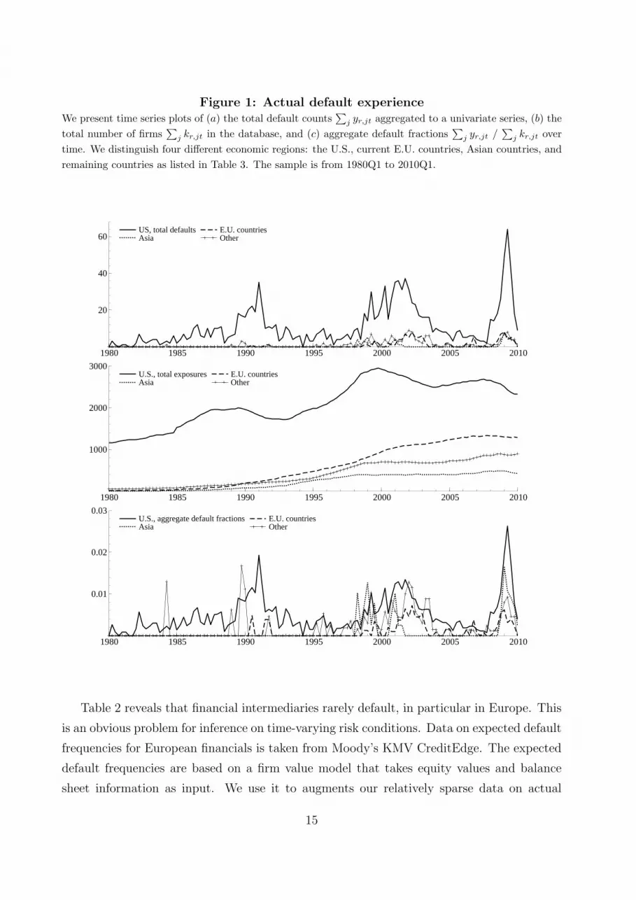
Figure 1: Actual default experienceWe present time series plots of (a) the total default counts

∑j yr,jt aggregated to a univariate series, (b) the

total number of firms∑

j kr,jt in the database, and (c) aggregate default fractions∑

j yr,jt /∑

j kr,jt overtime. We distinguish four different economic regions: the U.S., current E.U. countries, Asian countries, andremaining countries as listed in Table 3. The sample is from 1980Q1 to 2010Q1.

US, total defaults Asia

E.U. countries Other

1980 1985 1990 1995 2000 2005 2010

20

40

60US, total defaults Asia

E.U. countries Other

U.S., total exposures Asia

E.U. countries Other

1980 1985 1990 1995 2000 2005 2010

1000

2000

3000U.S., total exposures Asia

E.U. countries Other

U.S., aggregate default fractions Asia

E.U. countries Other

1980 1985 1990 1995 2000 2005 2010

0.01

0.02

0.03U.S., aggregate default fractions Asia

E.U. countries Other

Table 2 reveals that financial intermediaries rarely default, in particular in Europe. This

is an obvious problem for inference on time-varying risk conditions. Data on expected default

frequencies for European financials is taken from Moody’s KMV CreditEdge. The expected

default frequencies are based on a firm value model that takes equity values and balance

sheet information as input. We use it to augments our relatively sparse data on actual

15

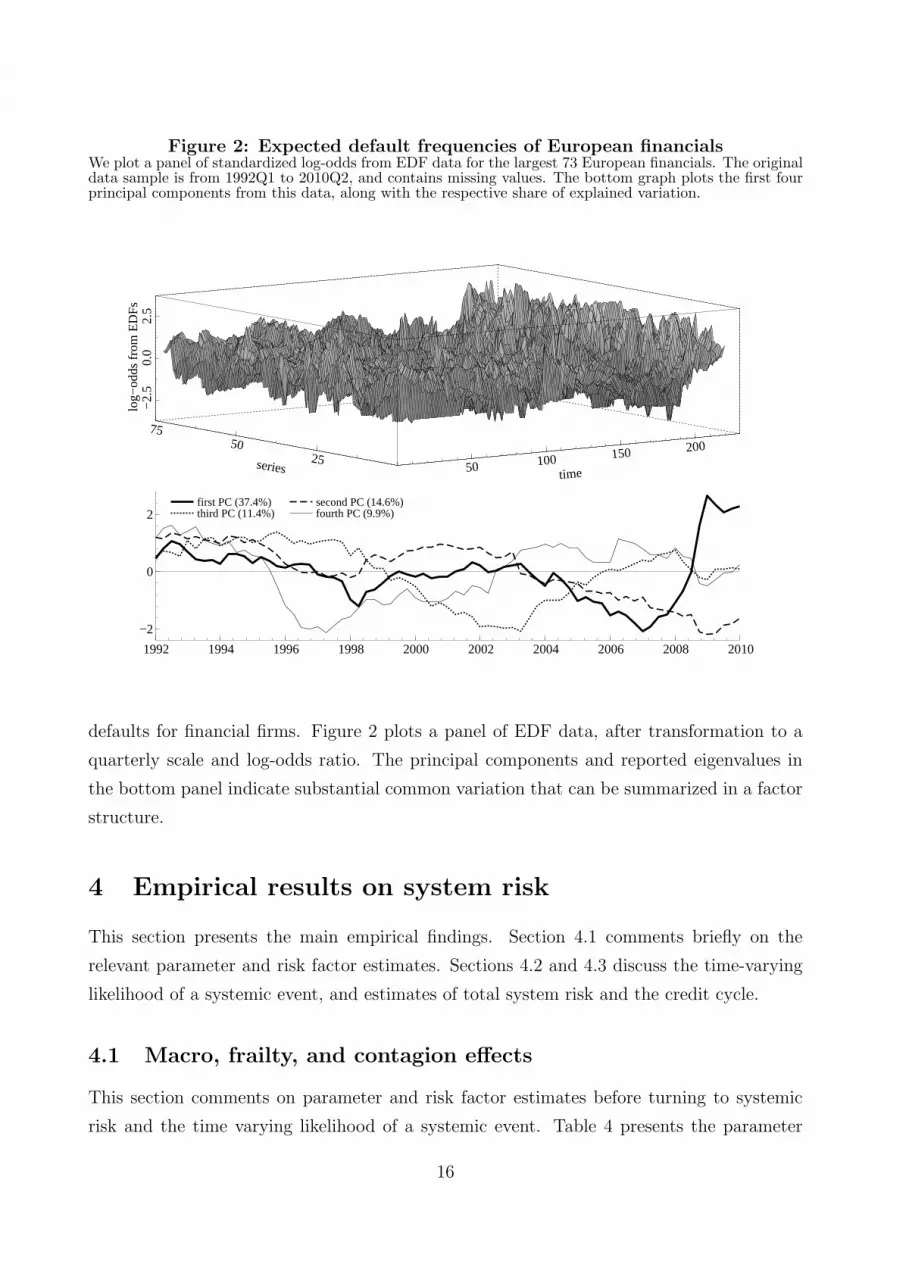
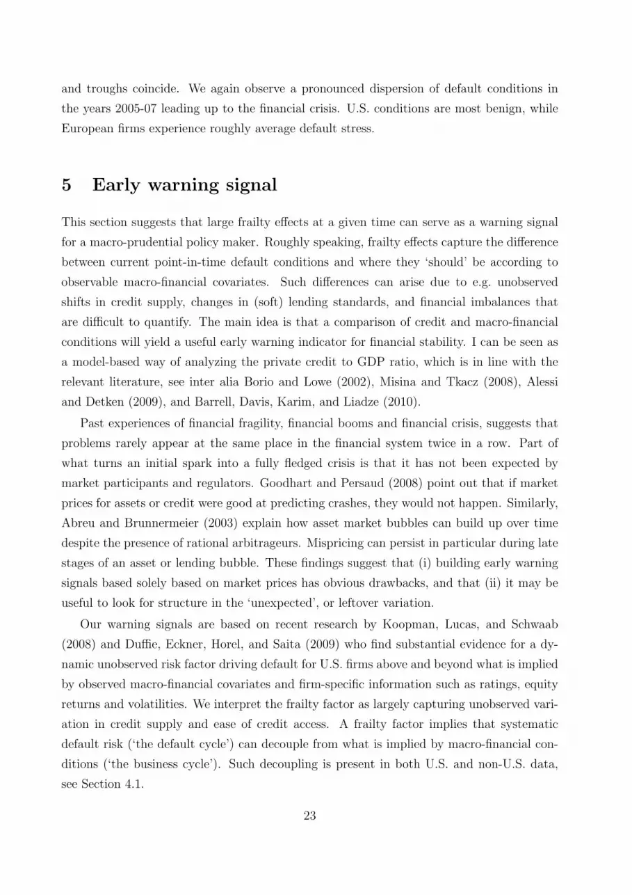
Figure 2: Expected default frequencies of European financialsWe plot a panel of standardized log-odds from EDF data for the largest 73 European financials. The originaldata sample is from 1992Q1 to 2010Q2, and contains missing values. The bottom graph plots the first fourprincipal components from this data, along with the respective share of explained variation.

timeseries

log−

odds

from

ED

Fs

50 100 150 20025

5075

−2.

50.

02.

5

first PC (37.4%) third PC (11.4%)

second PC (14.6%) fourth PC (9.9%)

1992 1994 1996 1998 2000 2002 2004 2006 2008 2010

−2

0

2first PC (37.4%) third PC (11.4%)

second PC (14.6%) fourth PC (9.9%)

defaults for financial firms. Figure 2 plots a panel of EDF data, after transformation to a

quarterly scale and log-odds ratio. The principal components and reported eigenvalues in

the bottom panel indicate substantial common variation that can be summarized in a factor

structure.

4 Empirical results on system risk

This section presents the main empirical findings. Section 4.1 comments briefly on the

relevant parameter and risk factor estimates. Sections 4.2 and 4.3 discuss the time-varying

likelihood of a systemic event, and estimates of total system risk and the credit cycle.

4.1 Macro, frailty, and contagion effects

This section comments on parameter and risk factor estimates before turning to systemic

risk and the time varying likelihood of a systemic event. Table 4 presents the parameter

16

Figure 3: Default intensities non-financial firmsWe plot model-implied discrete time default intensities for six broad non-financial industry sectors. Wedistinguish U.S., EU-27, and Other firms. Estimation sample is 1981Q1 to 2010Q1.

Transportation, US EU Other

1985 1990 1995 2000 2005 2010

5

10 Transportation, US EU Other

Leisure, US EU Other

1985 1990 1995 2000 2005 2010

5

10 Leisure, US EU Other

Energy, US EU Other

1985 1990 1995 2000 2005 2010

1

2 Energy, US EU Other

Industrials, US EU Other

1985 1990 1995 2000 2005 2010

1

2

3

4Industrials, US EU Other Technology, US EU Other

1985 1990 1995 2000 2005 2010

1

2

3Technology, US EU Other

Consumer goods & retail, US EU Other

1985 1990 1995 2000 2005 2010

1

2

3Consumer goods & retail, US EU Other

estimates for model specification (1) to (12). The fixed effects and factor loadings in the signal

equation (9) adhere to the additive structure (11). Coefficients λ in the left column combine

to baseline hazard rates. The middle and right columns present estimates for loadings β, γ,

and δ that pertain to macro, frailty, and industry (contagion) factors, respectively.

We find that macro, frailty, and contagion effects are all important for credit risk con-

ditions. Defaults from all regions load significantly on common factors from macro and

financial data, which by itself already implies a considerable degree of default clustering.

In general, however, common variation with macro data is not sufficient. Frailty effects are

particularly pronounced for U.S. and Asian firms. Latent industry-specific factors load on

default data from all regions.

We omit graphs of latent macro and industry risk factors for space considerations. The

macro, frailty, and industry-specific factor estimates combine to imply default rates at the

international and industry level. Figure 3 plots estimated default hazard rates for six non-

financial broad industry groups. Hazard rates tend to be lower for European and Asian

firms, reflecting higher credit ratings on average, see the bottom panel of Table 3. The

17

Table 4: Parameter estimatesWe report the maximum likelihood estimates of selected coefficients in the specification of the log-odds ratio(9) with parameterization (11) for λ and β. Coefficients λ combine to fixed effects, or baseline hazard rates.Factor loadings β, γ, δ, and κ refer to macro, frailty, industry (contagion), and observed risk factors, respec-tively. Monte Carlo log-likelihood evaluation is based on M = 5000 importance samples. The estimationsample is from 1981Q1 to 2010Q1.

Intercepts λj Loadings fmt Loadings fd

t , f it , ct

par val t-valλ0 -2.67 11.56

λ1,fin 0.14 0.54λ1,tra -0.29 0.73λ1,lei -0.04 0.24λ1,utl -0.27 0.84λ1.tec -0.04 0.23λ1,ret -0.40 2.49

λ2,IG -7.67 12.24λ2,BB -3.78 10.03λ2,B -2.27 14.19

λ3,EU -1.23 5.45λ3,AS -1.80 3.00λ3,Ot -1.51 1.55

par val t-valβ1,0 0.34 3.60β1,1,fin 0.02 0.11β1,2,IG 0.78 2.18β1,3,EU 0.26 0.92β1,3,Ot 0.38 1.45

β2,0 0.21 1.75β2,1,fin 0.08 0.53β2,2,IG -0.11 0.39β2,3,EU 0.10 0.37β2,3,Ot 0.01 0.01

β3,0 -0.05 0.44β3,1,fin -0.09 0.62β3,2,IG 0.33 1.24β3,3,EU -0.34 1.04β3,3,Ot 0.13 0.18

β4,0 -0.11 1.44β4,1,fin -0.05 0.36β4,2,IG 0.92 3.65β4,3,EU -0.01 0.62β4,3,Ot -0.57 1.12

par val t-valγUS 0.51 6.71γEU 0.05 0.07γOT 0.25 1.91

δfin 0.45 2.35δtra 0.72 2.84δlei 0.40 1.54δutl 0.99 2.34δind - -δtec 0.54 1.77δret 0.48 2.28

18

Figure 4: Implied financial sector default intensityWe plot the model-implied default intensities for financial sector firms (i.e., banks and financial non-banks).Estimation sample is 1981Q1 to 2010Q1.

Financials, US EU−27 Other

1985.0 1987.5 1990.0 1992.5 1995.0 1997.5 2000.0 2002.5 2005.0 2007.5 2010.0

0.5

1.0

Financials, US EU−27 Other

recent financial crisis of 2008-09 is clearly visible in most industry segments. The default

stress following the dot-com asset price bubble burst in 2000 can be seen for technology

firms during 2001-02. The model-implied default rate volatility is striking. Point-in-time

default hazard rates are five times (transportation, industrials) and up to ten times (e.g.

consumer goods & retail) higher in bad times than in good times, in all regions. This

substantial variation in non-financial default hazard rates, and the associated significant

degree of default clustering, implies time-varying financial stress on institutions that extend

credit to these firms. As a result, non-financial credit risk conditions help to infer the level

of financial firms’ distress.

4.2 The conditional probability of a systemic event

In this subsection, we define a systemic event as the failure of a large number of financial

intermediaries such as depository institutions, insurers, re-insurers, and broker/dealers. The

latter three categories are financial non-banks, and constitute the ‘shadow’ banking system.

System risk is narrowly defined as the time-varying conditional probability of experiencing

a systemic event, as in Giesecke and Kim (2010). The probability of joint financial failure is

closely related to the estimated default intensity for financial firms.

Figure 4 plots the estimated financial sector default intensity. The values range from

slightly above zero in good times to about 1% in a crisis in the U.S. That means that

financial crisis distress is such that roughly 1% of the financial sector should be expected

to ‘die’ over the next three months if no intervention takes place. With roughly 700 rated

financial firms in the U.S. and E.U. around 2008 (see Table 3), a 1% sector default intensity

19

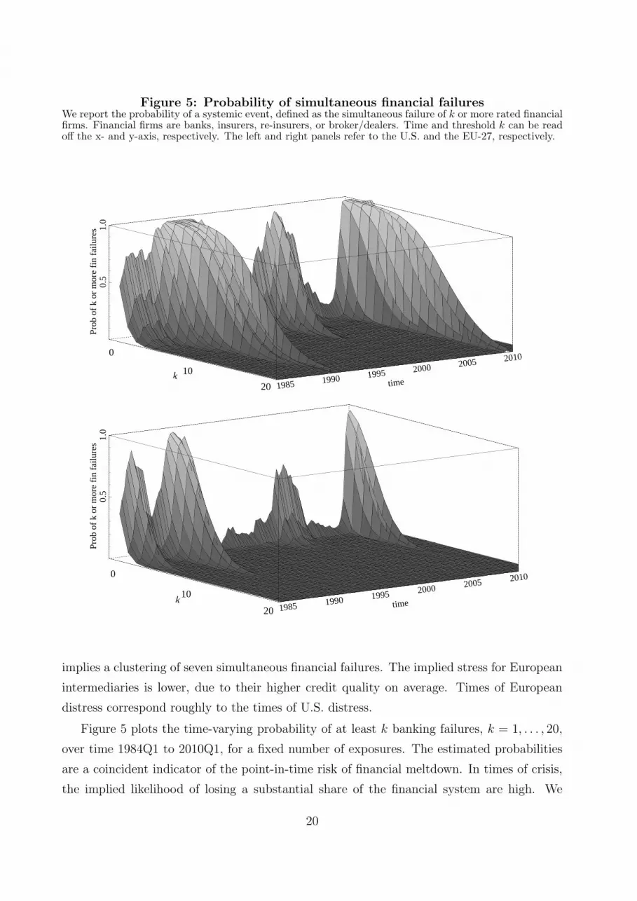
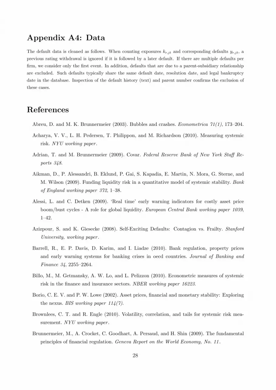
Figure 5: Probability of simultaneous financial failuresWe report the probability of a systemic event, defined as the simultaneous failure of k or more rated financialfirms. Financial firms are banks, insurers, re-insurers, or broker/dealers. Time and threshold k can be readoff the x- and y-axis, respectively. The left and right panels refer to the U.S. and the EU-27, respectively.

timek

Prob

of

k or

mor

e fi

n fa

ilure

s

0

10

1985 1990 1995 2000 2005 2010

0.5

1.0

timek

Prob

of

k or

mor

e fi

n fa

ilure

s

20

0

10

20 1985 1990 1995 2000 2005 2010

0.5

1.0

implies a clustering of seven simultaneous financial failures. The implied stress for European

intermediaries is lower, due to their higher credit quality on average. Times of European

distress correspond roughly to the times of U.S. distress.

Figure 5 plots the time-varying probability of at least k banking failures, k = 1, . . . , 20,

over time 1984Q1 to 2010Q1, for a fixed number of exposures. The estimated probabilities

are a coincident indicator of the point-in-time risk of financial meltdown. In times of crisis,

the implied likelihood of losing a substantial share of the financial system are high. We

20

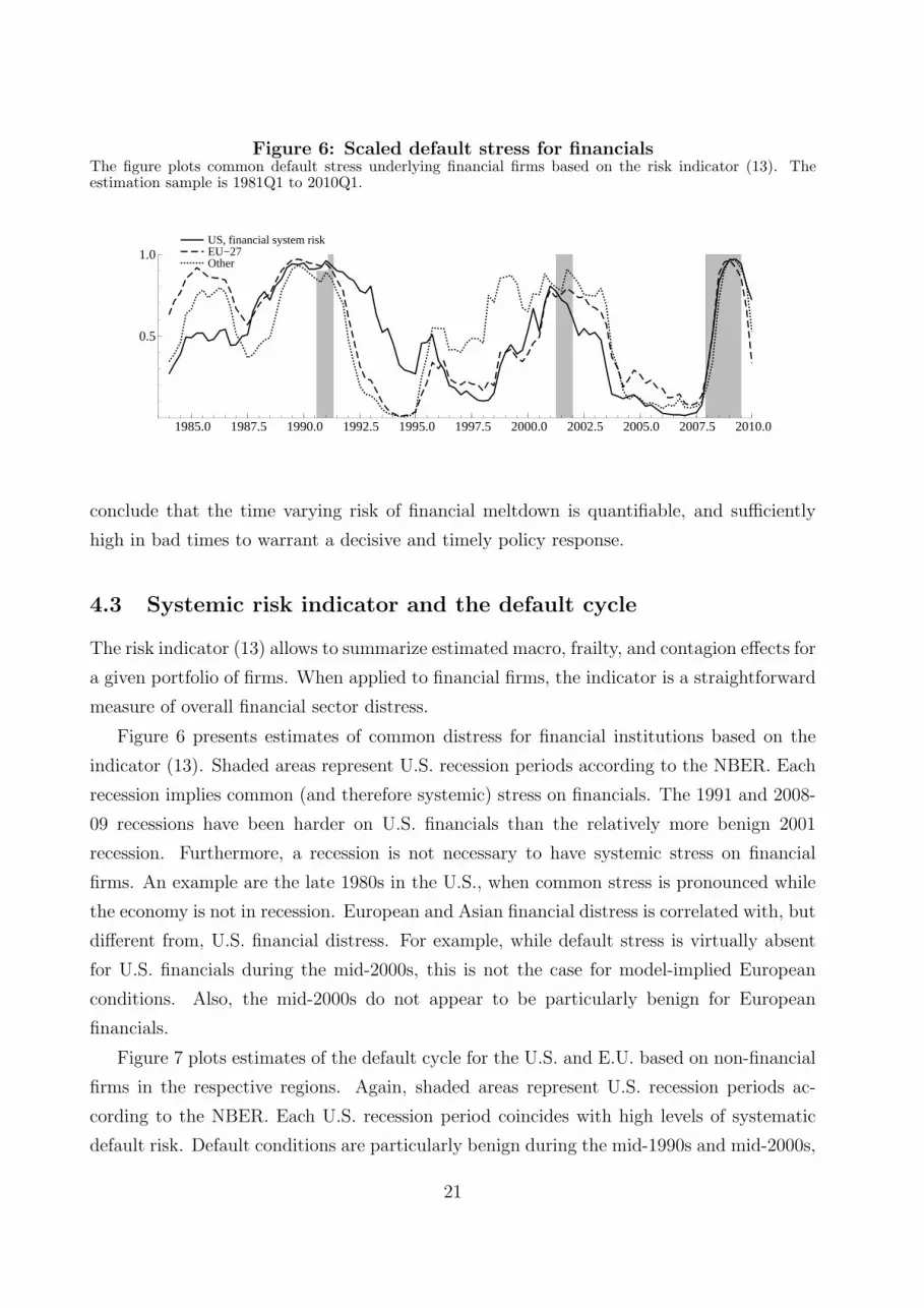
Figure 6: Scaled default stress for financialsThe figure plots common default stress underlying financial firms based on the risk indicator (13). Theestimation sample is 1981Q1 to 2010Q1.

US, financial system risk EU−27 Other

1985.0 1987.5 1990.0 1992.5 1995.0 1997.5 2000.0 2002.5 2005.0 2007.5 2010.0

0.5

1.0US, financial system risk EU−27 Other

conclude that the time varying risk of financial meltdown is quantifiable, and sufficiently

high in bad times to warrant a decisive and timely policy response.

4.3 Systemic risk indicator and the default cycle

The risk indicator (13) allows to summarize estimated macro, frailty, and contagion effects for

a given portfolio of firms. When applied to financial firms, the indicator is a straightforward

measure of overall financial sector distress.

Figure 6 presents estimates of common distress for financial institutions based on the

indicator (13). Shaded areas represent U.S. recession periods according to the NBER. Each

recession implies common (and therefore systemic) stress on financials. The 1991 and 2008-

09 recessions have been harder on U.S. financials than the relatively more benign 2001

recession. Furthermore, a recession is not necessary to have systemic stress on financial

firms. An example are the late 1980s in the U.S., when common stress is pronounced while

the economy is not in recession. European and Asian financial distress is correlated with, but

different from, U.S. financial distress. For example, while default stress is virtually absent

for U.S. financials during the mid-2000s, this is not the case for model-implied European

conditions. Also, the mid-2000s do not appear to be particularly benign for European

financials.

Figure 7 plots estimates of the default cycle for the U.S. and E.U. based on non-financial

firms in the respective regions. Again, shaded areas represent U.S. recession periods ac-

cording to the NBER. Each U.S. recession period coincides with high levels of systematic

default risk. Default conditions are particularly benign during the mid-1990s and mid-2000s,

21

Figure 7: Scaled default stress for non-financialsThe figure plots common default stress underlying non-financial corporates based on the systematic riskindicator (13). Estimation sample is 1981Q1 to 2010Q1.

US, non−financial default cycle EU−27 Other

1985.0 1987.5 1990.0 1992.5 1995.0 1997.5 2000.0 2002.5 2005.0 2007.5 2010.0

0.5

1.0

US, non−financial default cycle EU−27 Other

with values about 0.25 on a scale from zero to one. The mid-1990s are associated with the

Clinton-Greenspan policy mix of low interest rates and low budget deficits, and correspond-

ing favorable macroeconomic conditions. The mid-2000s are characterized by exceptionally

low interest rates and easy credit access for U.S. firms. U.S. default conditions are more

benign compared to E.U. conditions during the years 2005-07 leading up to the recent crisis.

This may reflect direct and indirect effects from more aggressive interest rate cuts by the

Federal Reserve compared to other central banks in these years, see e.g. Taylor (2008).

Figure 8 plots the model-implied world credit cycle using (13) as well as regional de-

viations from the world cycle. The regional cycles are highly correlated. The main peaks

Figure 8: World credit cycle and regional deviationsWe plot a world credit cycle estimate based on the indicator (13) and point-in-time default hazard ratesfor all (financial and non-financial) firms in each region. Regional credit cycle conditions are plotted forcomparison.

World conditions US EU−27 Other

1985.0 1987.5 1990.0 1992.5 1995.0 1997.5 2000.0 2002.5 2005.0 2007.5 2010.0

0.5

1.0 World conditions US EU−27 Other

22

and troughs coincide. We again observe a pronounced dispersion of default conditions in

the years 2005-07 leading up to the financial crisis. U.S. conditions are most benign, while

European firms experience roughly average default stress.

5 Early warning signal

This section suggests that large frailty effects at a given time can serve as a warning signal

for a macro-prudential policy maker. Roughly speaking, frailty effects capture the difference

between current point-in-time default conditions and where they ‘should’ be according to

observable macro-financial covariates. Such differences can arise due to e.g. unobserved

shifts in credit supply, changes in (soft) lending standards, and financial imbalances that

are difficult to quantify. The main idea is that a comparison of credit and macro-financial

conditions will yield a useful early warning indicator for financial stability. I can be seen as

a model-based way of analyzing the private credit to GDP ratio, which is in line with the

relevant literature, see inter alia Borio and Lowe (2002), Misina and Tkacz (2008), Alessi

and Detken (2009), and Barrell, Davis, Karim, and Liadze (2010).

Past experiences of financial fragility, financial booms and financial crisis, suggests that

problems rarely appear at the same place in the financial system twice in a row. Part of

what turns an initial spark into a fully fledged crisis is that it has not been expected by

market participants and regulators. Goodhart and Persaud (2008) point out that if market

prices for assets or credit were good at predicting crashes, they would not happen. Similarly,

Abreu and Brunnermeier (2003) explain how asset market bubbles can build up over time

despite the presence of rational arbitrageurs. Mispricing can persist in particular during late

stages of an asset or lending bubble. These findings suggest that (i) building early warning

signals based solely based on market prices has obvious drawbacks, and that (ii) it may be

useful to look for structure in the ‘unexpected’, or leftover variation.

Our warning signals are based on recent research by Koopman, Lucas, and Schwaab

(2008) and Duffie, Eckner, Horel, and Saita (2009) who find substantial evidence for a dy-

namic unobserved risk factor driving default for U.S. firms above and beyond what is implied

by observed macro-financial covariates and firm-specific information such as ratings, equity

returns and volatilities. We interpret the frailty factor as largely capturing unobserved vari-

ation in credit supply and ease of credit access. A frailty factor implies that systematic

default risk (‘the default cycle’) can decouple from what is implied by macro-financial con-

ditions (‘the business cycle’). Such decoupling is present in both U.S. and non-U.S. data,

see Section 4.1.

23

Figure 9: Frailty factor estimatesWe plot the conditional mean estimates of region-specific frailty factors with 95% standard error bands.

US, cond mean frailty factor 0.95 std error band

1985 1990 1995 2000 2005 2010

−2.5

0.0

2.5

US, cond mean frailty factor 0.95 std error band

EU−27, cond mean frailty factor 0.95 std error band

1985 1990 1995 2000 2005 2010

−2.5

0.0

2.5

EU−27, cond mean frailty factor 0.95 std error band

Other countries, cond mean frailty factor 0.95 std error band

1985 1990 1995 2000 2005 2010

−2.5

0.0

2.5

Other countries, cond mean frailty factor 0.95 std error band

Figure 9 presents the estimated frailty factors for the U.S., EU-27, and the rest of the

world. For the U.S., frailty effects have been pronounced during bad times, such as the

savings and loan crisis in the U.S. in the late 1980s, leading up to the 1991 recession. They

have also been pronounced in exceptionally good times, such as the years 2005-07 leading

up to the recent financial crisis. In these years, default conditions are much more benign

than would be expected from observed macro and financial data. Frailty effects are large in

absolute value, and significantly different from zero at these times. As expected from Table

4, European frailty effects are not significant in most of the observed history. However,

all frailty factors are similar negative during the pre-crisis period. This suggests a similar

build-up of systematic risk in all areas during this time.

6 Conclusion

We proposed a novel diagnostic framework for financial systemic risk assessment based on

state space methods. A nonlinear non-Gaussian factor model allows us to assess latent macro-

24

financial and credit risk conditions in different economic regions. The factor estimates can

be combined into a new and straightforward indicator of financial system risk. A decoupling

of credit from macro-financial conditions may serve as an early warning signal for a macro-

prudential policy maker.

Appendix A1: estimation via importance sampling

An analytical expression for the the maximum likelihood (ML) estimate of the parameter vector is not

available for model formulation (2) to (12). A feasible approach to the ML estimation of model parameters ψ

is the maximization of the likelihood function that is evaluated via Monte Carlo methods such as importance

sampling. A short description of this approach is given below. A full treatment is presented by Durbin and

Koopman (2001, Part II).

The observation density function of y = (y′1, x′1, . . . , y

′T , x′T )′ can be expressed by the joint density of y

and f = (f ′1, . . . , f′T )′ where f is integrated out, that is

p(y; ψ) =∫

p(y, f ;ψ)df =∫

p(y|f ; ψ)p(f ; ψ)df, (A.14)

where p(y|f ; ψ) is the density of y conditional on f and p(f ; ψ) is the density of f . A Monte Carlo estimator

of p(y; ψ) can be obtained by

p(y; ψ) = M−1M∑

k=1

p(y|f (k); ψ), f (k) ∼ p(f ; ψ),

for some large integer M . The estimator p(y; ψ) is however numerically inefficient since most draws f (k) will

not contribute substantially to p(y|f ; ψ) for any ψ and k = 1, . . . , K. Importance sampling improves the

Monte Carlo estimation of p(y; ψ) by sampling f from the Gaussian importance density g(f |y;ψ). We can

express the observation density function p(y;ψ) by

p(y;ψ) =∫

p(y, f ;ψ)g(f |y;ψ)

g(f |y; ψ)df = g(y; ψ)∫

p(y|f ; ψ)g(y|f ; ψ)

g(f |y;ψ)df. (A.15)

Since f is from a Gaussian density, we have g(f ;ψ) = p(f ; ψ) and g(y; ψ) = g(y, f ; ψ) / g(f |y; ψ). In case

g(f |y;ψ) is close to p(f |y; ψ) and in case simulation from g(f |y; ψ) is feasible, the Monte Carlo estimator

p(y; ψ) = g(y; ψ)M−1M∑

k=1

p(y|f (k); ψ)g(y|f (k); ψ)

, f (k) ∼ g(f |y;ψ), (A.16)

is numerically much more efficient, see Kloek and van Dijk (1978), Geweke (1989) and Durbin and Koopman

(2001).

For a practical implementation, the importance density g(f |y; ψ) can be based on the linear Gaussian

approximating model

yjt = µjt + θjt + εjt, εjt ∼ N(0, σ2jt), (A.17)

where mean correction µjt and variance σ2jt are determined in such a way that g(f |y; ψ) is sufficiently close

25

to p(f |y; ψ). It is argued by Shephard and Pitt (1997) and Durbin and Koopman (1997) that µjt and σjt

can be uniquely chosen such that the modes of p(f |y;ψ) and g(f |y;ψ) with respect to f are equal, for a

given value of ψ.

To simulate values from the importance density g(f |y; ψ), the simulation smoothing method of Durbin

and Koopman (2002) can be applied to the approximating model (A.17). For a set of M draws of g(f |y;ψ),

the evaluation of (A.16) relies on the computation of p(y|f ;ψ), g(y|f ; ψ) and g(y; ψ). Density p(y|f ; ψ) is

based on (5) and (4), density g(y|f ;ψ) is based on the Gaussian density for yjt−µjt− θjt ∼ N(0, σ2jt) (A.17)

and g(y; ψ) can be computed by the Kalman filter applied to (A.17), see Durbin and Koopman (2001).

The likelihood function can be evaluated for any value of ψ. For a given set of random numbers from

which factors are simulated from g(f |y; ψ), we maximize the likelihood (A.16) with respect to ψ.

Furthermore, we can estimate the latent factors ft via importance sampling. It can be shown that

E(f |y; ψ) =∫

f · p(f |y; ψ)df =∫

f · w(y, f ; ψ)g(f |y; ψ)df∫w(y, f ; ψ)g(f |y; ψ)df

,

where w(y, f ;ψ) = p(y|f ; ψ)/g(y|f ; ψ). The estimation of E(f |y; ψ) via importance sampling can be achieved

by

f =M∑

k=1

wk · f (k)

/M∑

k=1

wk,

with wk = p(y|f (k);ψ)/g(y|f (k);ψ), and f (k) ∼ g(f |y;ψ). Similarly, the standard errors st of ft can be

estimated by

s2t =

(M∑

k=1

wk · (f (k)t )2

/M∑

k=1

wk

)− f2

t ,

with ft the tth elements of f . Conditional mode estimates of the factors are given by

f = argmax p(f |y; ψ), (A.18)

and indicate the most probable value of the factors given the observations. They are obtained as a by-product

when matching the modes of densities p(f |y;ψ) and g(f |y;ψ).

Appendix A2: treatment of missing values

Missing values can be accommodated relatively easily in a state space approach. Most implementations of

the Kalman filter (KF) and associated smoother (KFS) deal with them automatically, see e.g. Koopman,

Shephard, and Doornik (2008). Some care must be taken when computing the importance sample weights

wk = p(y|f (k);ψ)/g(y|f (k); ψ), f (k) ∼ g(f |y;ψ). While y = (y′1, . . . , y′T )′ may contain many missing values,

the (mode) estimates of the corresponding signals θ = (θ′1, . . . , θ′T )′ and factors f = (f ′1, . . . , f

′T )′ are available

for all data. Some bookkeeping is therefore required to evaluate p(y|f ;ψ) and g(y|f ;ψ) at the corresponding

values of f , or θ.

Missing values also arise at the end of the sample when forecasting the latent risk factors. Forecasts

fT+h, for h = 1, 2, . . . , H, can be obtained by treating future observations yT+1, . . . , yt+H as missing, and

applying the estimation and signal extraction techniques of Section 6 to data (y0, . . . , yT+H). The obtained

conditional mean f and mode forecasts f of the factors provide a location and maximum-probability forecast

26

given observations, respectively. The mean (or median, mode) predictions of observations (yT+1, . . . , yT+H)

can be obtained as nonlinear functions of (fT+1, . . . , fT+H).

Appendix A3: collapsing observations

A recent result in Jungbacker and Koopman (2008) states that it is possible to collapse a [N × 1] vector of

(Gaussian) observations yt into a vector of transformed observations ylt of lower dimension m < N without

compromising the information required to estimate factors ft via the Kalman Filter and Smoother. We

here adapt their argument to a nonlinear mixed-measurement setting. We focus on collapsing the artificial

Gaussian data yt with associated covariance matrices Ht, see (A.17) and (12).

Consider a linear approximating model for transformed data y∗t = Atyt, for a sequence of invertible

matrices At, for t = 1, . . . , T . The transformed observations are given by

y∗t =

(yl

t

yht

), with yl

t = Altyt and yh

t = Aht yt,

where time-varying projection matrices are partitioned as At =[Al′

t : Ah′t

]′. We require (i) matrices At to be

of full rank to prevent the loss of information in each rotation, (ii) Aht HtA

l′t = 0 to ensure that observations

ylt and yh

t are independent, and (iii) Aht Zt = 0 to ensure that yh

t does not depend on f . Several such matrices

Alt that fulfill these conditions can be found. A convenient choice is presented below. Matrices Ah

t can be

constructed from Alt, but are not necessary for computing smoothed signal and factor estimates.

Given matrices At, a convenient model for transformed observations y∗t is of the form

ylt = Al

tθt + elt,

yht = eh

t

,

(elt

eht

)∼ NIID

(0,

[H l

t 0

0 Hht

]),

where H lt = Al

tHtAl′t , Hh

t = Aht HtA

h′t , θt = Zft, and Z contains the factor loadings. Clearly, the [N −m]

dimensional vector yht contains no information about ft. We can speed up computations involving the KFS

recursions as follows.

Algorithm : Consider (approximating) Gaussian data yt with time-varying covariance matrices Ht, and

N > m. To compute smoothed factors ft and signals θt,

1. construct, at each time t = 1, . . . , T , a matrix Alt = CtZ

′H−1t , with Ct such that C ′tCt =

(Z ′H−1

t Z)−1

and Ct upper triangular. Collapse observations as ylt = Al

tyt.

2. apply the Kalman Filter and Smoother (KFS) to the [m × 1] low-dimensional vector ylt with time-

varying factor loadings C−1′t and H l

t = Im.

This approach gives the same factor and signal estimates as when the KFS recursions are applied to the

[N × 1] dimensional system for yt with factor loadings Z and covariances Ht.

A derivation is provided in Jungbacker and Koopman (2008, Illustration 4).

27

Appendix A4: Data

The default data is cleaned as follows. When counting exposures kr,jt and corresponding defaults yr,jt, a

previous rating withdrawal is ignored if it is followed by a later default. If there are multiple defaults per

firm, we consider only the first event. In addition, defaults that are due to a parent-subsidiary relationship

are excluded. Such defaults typically share the same default date, resolution date, and legal bankruptcy

date in the database. Inspection of the default history (text) and parent number confirms the exclusion of

these cases.

References

Abreu, D. and M. K. Brunnermeier (2003). Bubbles and crashes. Econometrica 71(1), 173–204.

Acharya, V. V., L. H. Pedersen, T. Philippon, and M. Richardson (2010). Measuring systemic

risk. NYU working paper .

Adrian, T. and M. Brunnermeier (2009). Covar. Federal Reserve Bank of New York Staff Re-

ports 348.

Aikman, D., P. Alessandri, B. Eklund, P. Gai, S. Kapadia, E. Martin, N. Mora, G. Sterne, and

M. Wilson (2009). Funding liquidity risk in a quantitative model of systemic stability. Bank

of England working paper 372, 1–38.

Alessi, L. and C. Detken (2009). ‘Real time’ early warning indicators for costly asset price

boom/bust cycles - A role for global liquidity. European Central Bank working paper 1039,

1–42.

Azizpour, S. and K. Giesecke (2008). Self-Exciting Defaults: Contagion vs. Frailty. Stanford

University, working paper .

Barrell, R., E. P. Davis, D. Karim, and I. Liadze (2010). Bank regulation, property prices

and early warning systems for banking crises in oecd countries. Journal of Banking and

Finance 34, 2255–2264.

Billo, M., M. Getmansky, A. W. Lo, and L. Pelizzon (2010). Econometric measures of systemic

risk in the finance and insurance sectors. NBER working paper 16223.

Borio, C. E. V. and P. W. Lowe (2002). Asset prices, financial and monetary stability: Exploring

the nexus. BIS working paper 114(7).

Brownlees, C. T. and R. Engle (2010). Volatility, correlation, and tails for systemic risk mea-

surement. NYU working paper .

Brunnermeier, M., A. Crocket, C. Goodhart, A. Persaud, and H. Shin (2009). The fundamental

principles of financial regulation. Geneva Report on the World Economy, No. 11 .

28

Brunnermeier, M. K. (2009). Deciphering the liquidity and credit crunch 20072008. Journal of

Economic Perspectives 23(1), 77–100.

Creal, D., B. Schwaab, S. J. Koopman, and A. Lucas (2010). Mixed measurement dynamic factor

models. working paper, available at www.tinbergen.nl/∼bschwaab.

Das, S., D. Duffie, N. Kapadia, and L. Saita (2007). Common Failings: How Corporate Defaults

Are Correlated. The Journal of Finance 62(1), 93–117(25).

de Larosiere, J. (2009). The high level group on financial supervision in the E.U. - Report.

Bruxelles: The European Commission.

Duffie, D., A. Eckner, G. Horel, and L. Saita (2009). Frailty Correlated Default. Journal of

Finance 64(5), 2089–2123.

Durbin, J. and S. J. Koopman (1997). Monte Carlo Maximum Likelihood estimation for non-

Gaussian State Space Models. Biometrica 84(3), 669–684.

Durbin, J. and S. J. Koopman (2001). Time Series Analysis by State Space Methods. Oxford:

Oxford University Press.

Durbin, J. and S. J. Koopman (2002). A simple and efficient simulation smoother for state space

time series analysis. Biometrika 89(3), 603–616.

ECB (2009). The concept of systemic risk. European Central Bank Financial Stability Review,

December 2009 .

ECB (2010). Analytical models and tools for the identification and assessment of systemic risks.

European Central Bank Financial Stability Review, June 2010 .

Geweke, J. (1989). Bayesian inference in econometric models using Monte Carlo integration.

Econometrica 57, 1317–39.

Giesecke, K. and B. Kim (2010). Systemic risk: What defaults are telling us. Stanford University

working paper , 1–34.

Goodhart, C. and A. Persaud (2008). A proposal for how to avoid the next crash. Financial

Times UK, 31 Jan 2008 .

Goodhart, C. A. E., P. Sunirand, and D. P. Tsomocos (2006). A model to analyse financial

fragility. Annals of Finance 2(1), 1–21.

Hartmann, P., O. de Bandt, and J. L. P. Alcalde (2009). Systemic risk in banking: An update.

Oxford Handbook of Banking, ed. by A. Berger, P. Molyneux and J. Wilson, Oxford University

Press.

Hartmann, P., S. Straetmans, and C. de Vries (2005). Banking system stability: A cross-atlantic

perspective. NBER working paper 11698, 1–86.

29

Jungbacker, B. and S. J. Koopman (2008). Likelihood-based Analysis of Dynamic Factor Models.

Tinbergen Institute Discussion Paper .

Kloek, T. and H. K. van Dijk (1978). Bayesian estimates of equation system parameters: an

application of integration by Monte Carlo. Econometrica 46, 1–20.

Koopman, S. J. and A. Lucas (2008). A Non-Gaussian Panel Time Series Model for Estimating

and Decomposing Default Risk. Journal of Business and Economic Statistics 26 (4), 510–525.

Koopman, S. J., A. Lucas, and A. Monteiro (2008). The Multi-Stage Latent Factor Intensity

Model for Credit Rating Transitions. Journal of Econometrics 142(1), 399–424.

Koopman, S. J., A. Lucas, and B. Schwaab (2008). Forecasting Cross-sections of Frailty-

correlated Default. Tinbergen Institute Discussion Paper 029/04, 1–38.

Koopman, S. J., A. Lucas, and B. Schwaab (2010). Macro, frailty, and contagion effects in

defaults: Lessons from the 2008 credit crisis. Tinbergen Institute Discussion Paper 2010-

004/2, 1–40.

Koopman, S. J., N. Shephard, and J. A. Doornik (2008). Statistical Algorithms for Models in

State Space Form: Ssfpack 3.0. Timberlake Consultants Press, London.

Lando, D. (2003). Credit Risk Modelling - Theory and Applications. Princeton University Press.

Lando, D. and M. S. Nielsen (2008). Correlation in corporate defaults: Contagion or conditional

independence. Copenhagen Business School, working paper .

McNeil, A. and J. Wendin (2007). Bayesian inference for generalized linear mixed models of

portfolio credit risk. Journal of Empirical Finance 14(2), 131–149.

Misina, M. and G. Tkacz (2008). Credit, asset prices, and financial stress in canada. Bank of

Canada working paper 2008-10, 1–29.

Philippon, T. (2009). An overview of the proposals to fix the financial system. Vox EU,

www.voxeu.org .

Segoviano, M. A. and C. Goodhart (2009). Banking stability measures. IMF Working Paper .

Shephard, N. and M. K. Pitt (1997). Likelihood analysis of non-Gaussian measurement time

series. Biometrica 84, 653–67.

Taylor, J. B. (2008). Monetary policy and the state of the economy. Testimony before the Com-

mittee on Financial Services, U.S. House of Representatives, February 26, 2008 .

Trichet, J.-C. (2009). Clare Distinguished Lecture in Economics and Public Policy. University

of Cambridge, 10 December 2009 .

Volcker, P. A., J. A. Frenkel, A. F. Neto, and T. Padoa-Schioppa (2009). Financial Reform: A

framework for financial stability. Washington D.C.: Group of 30.

30