the impact of systemic risk on the diversification benefits of a risk portfolio

Risks 2014, 2, 260-276; doi:10.3390/risks2030260OPEN ACCESS

risksISSN 2227-9091

www.mdpi.com/journal/risks

Article

The Impact of Systemic Risk on the Diversification Benefits of aRisk PortfolioMarc Busse 1, Michel Dacorogna 1 and Marie Kratz 2,*

1 SCOR SE, 26 General Guisan Quai, 8022 Zürich, Switzerland; E-Mails: [email protected] (M.B.);[email protected] (M.D.)

2 ESSEC Business School Paris, CREAR, av. Bernard Hirsch BP 50105,95021 Cergy-Pontoise Cedex, France

* Author to whom correspondence should be addressed; E-Mail: [email protected].

Received: 2 December 2013; in revised form: 15 May 2014 / Accepted: 17 June 2014 /Published: 9 July 2014

Abstract: Risk diversification is the basis of insurance and investment. It is thus crucialto study the effects that could limit it. One of them is the existence of systemic risk thataffects all of the policies at the same time. We introduce here a probabilistic approach toexamine the consequences of its presence on the risk loading of the premium of a portfolioof insurance policies. This approach could be easily generalized for investment risk. We seethat, even with a small probability of occurrence, systemic risk can reduce dramatically thediversification benefits. It is clearly revealed via a non-diversifiable term that appears in theanalytical expression of the variance of our models. We propose two ways of introducingit and discuss their advantages and limitations. By using both VaR and TVaR to computethe loading, we see that only the latter captures the full effect of systemic risk when itsprobability to occur is low.

Keywords: diversification; expected shortfall; investment risk; insurance premium; riskloading; risk measure; risk management; risk portfolio; stochastic model; systemic risk;value-at-risk

MSC classifications: 91B30; 91B70; 62P05

Risks 2014, 2 261

1. Introduction

Every financial crisis reveals the importance of systemic risk and, as a consequence, the lack ofdiversification. Diversification is a way to reduce the risk by detaining many different risks, with variousprobabilities of occurrence and a low probability of happening simultaneously. Unfortunately, in timesof crisis, most of the financial assets move together and become very correlated. The 2008/2009 crisis isnot an exception. It has highlighted the interconnectedness of financial markets when they all came to astand still for more than a month waiting for the authorities to restore confidence in the system (see, e.g.,the Systemic Risk Survey of the bank of England, available on-line). For any financial institution, it isimportant to be aware of the limits to diversification, while, for researchers in this field, studying themechanisms that hamper diversification is crucial for the understanding of the dynamics of the system(see, e.g., [1,2] and the references therein). Both risk management and research on risk would enhanceour capacity to survive the inevitable failures of diversification. A small fact, like turmoils in the U.S.sub-prime real-estate market, a relatively small market compared to the whole U.S. real-estate market,can trigger a major financial crisis that extends to all markets and all regions in the globe. Systemicrisk manifests itself by a breakdown of the diversification benefits and the appearance of dependencestructures that were not deemed important during normal times.

Since the crisis, the literature on this subject has been abundant. It mainly centers on two approaches.On one hand, there exist attempts to explain the appearance of systemic risk through structuralmacro-economic or financial models that include feedback loops and non-linear effects [2–7]. Onthe other hand, empirical indicators have been proposed to measure the danger of systemic risk inorder to provide early-warning systems [8–12]. While these studies are essential to progress in ourunderstanding of the economic factors leading to the emergence of economic crisis due to systemicrisk, our approach is to concentrate on the more fundamental underlying mathematical mechanismsthat break diversification. In the economic literature, systemic risk is identified with contagion effectsand the literature concentrates on finding ways of modeling or measuring it. One consequence of thiscontagion is the breaking of the law of large numbers and the sudden disappearance of the stabilizingeffect of diversification, joining here one of the main questions asked in quantitative risk management(see e.g. [13]). Another important subject of debate in the risk management literature is the controversyabout risk measures (see e.g. [14,15] and references therein). The aim of our study is precisely to lookat these aspects of the problem through a simple and didactic model. The question we want to answer is:are there simple mathematical mechanisms that break the law of large numbers and destroy the benefitsof diversification?

In this study, we introduce a simple stochastic modeling to understand and point out the limitationsto diversification and the mechanism leading to the occurrence of systemic risk. The idea is to combinetwo generating stochastic processes that, through their mixture, produces in the resulting process anon-diversifiable component, which we identify to be a systemic risk. Depending on the way of mixingthese processes, the diversification benefit appears with various strengths, due to the emergence of thesystemic component. The use of such a model, which is completely specified, allows us to obtainanalytical expressions for the variance and then to identify the non-diversifiable term. With the help of

Risks 2014, 2 262

Monte Carlo simulations, we explore the various components of the model and check that we reproducethe analytical results.

The paper is organized as follows: in the first section, we introduce, to measure the effects ondiversification, the standard insurance framework for pricing risk and define the risk measures that areused in this study. The second section is dedicated to the mathematical presentation of the model and itsvarious approaches to systemic risk, as well as numerical applications. The obtained results are comparednumerically and analytically in the third section, where we also discuss the influence of the choice ofthe risk measure on the diversification benefits. We conclude the study and suggest new perspectives toextend it.

2. Insurance Framework

Before moving to stochastic modeling, let us introduce the insurance framework in which we aregoing to compute the risk diversification. It is an example of application, but this study on systemic riskcould easily be generalized to any financial institution.

2.1. The Technical Risk Premium

In insurance, risk is priced based on the knowledge of the loss probability distribution. Let L be therandom variable (rv) representing a loss defined on a probability space (Ω, A, IP).

2.1.1. One policy case

For any policy incurring a loss L(1), we can define, as in [16], the technical premium, P , that needs tobe paid, as:

P = IE[L(1)] + ηK + e (1)

with η: the return expected by shareholders before tax, K: the risk capital assigned to this policy, e: theexpenses incurred by the insurer to handle this case.

An insurance company is a company in which we can invest. Therefore, the shareholders that haveinvested a certain amount of capital in the company expect a return on investment. Therefore, theinsurance firm has to make sure that the investors receive their dividends, which corresponds to thecost of capital the insurance company must charge on its premium. This is what we have called η.

We will assume that the expenses are a small portion of the expected loss:

e = aIE[L(1)] with 0 < a << 1

which transforms the premium as:

P = (1 + a)IE[L(1)] + ηK. (2)

We can now generalize this premium principle Equation (2) for N similar policies (or contracts).

Risks 2014, 2 263

2.1.2. The case of a portfolio of N policies

The premium for one policy in the portfolio, incurring now a total loss L(N) =∑N

i=1 L(1)i (where the

L(1)i ’s are N independent copies of L(1)), can then be written as

P =(1 + a)IE[L(N)] + ηKN

N= (1 + a) IE[L(1)] + η

KN

N

where KN is the capital assigned to the entire portfolio.

2.2. Cost of Capital and Risk Loading

First, we have to point out that the role of capital for an insurance company is to ensure that thecompany can pay its liability, even in the worst cases, up to some threshold. For this, we need to definethe capital that we have to put behind the risk. We are going to use a risk measure, say ρ, defined on theloss distribution. This allows us to estimate the capital needed to ensure the payment of the claim up toa certain confidence level. We then define the risk-adjusted-capital K as a function of the risk measure ρassociated with the risk1 L as:

K = ρ(L)− IE[L] (3)

since the risk is defined as the deviation from the expectation.Note that we could have also defined K as K = ρ(L) − IE[L] − P , since the premiums can serve to

pay the losses. This would change the premium P defined in Equation (1) into P defined by:

P =1 + a− η

1 + ηIE[L] +

η

1 + ηρ(L).

Such an alternative definition would reduce the capital, but does not change fundamentally the results ofthe study.

Consider a portfolio of N similar policies, using the notation for the loss as in Section 2.1. Let Rdenote the risk loading per policy, defined as the cost of the risk-adjusted capital per policy. UsingEquation (3), R can be expressed as a function of the risk measure ρ, namely:

R = ηKN

N= η

(ρ(L(N))

N− IE[L(1)]

). (4)

2.3. Risk Measures

We will consider for ρ two standard risk measures, the value-at-risk (VaR) and the tail value-at-risk(TVaR). Let us recall the definitions of these quantities (see, e.g., [17]).

The value-at-risk with a confidence level α is defined for a risk L by:

VaRα(L) = infq ∈ R : IP(L > q) ≤ 1− α = infq ∈ R : FL(q) ≥ α (5)

where q is the level of loss that corresponds to a VaRα (simply, the quantile of L of order α) and FLthe cdf of L.

1 We use here the word “risk” instead of “loss”. In fact, these two words are used for one another in an insurance context.

Risks 2014, 2 264

The tail value-at-risk at a confidence level α of L satisfies:

TVaRα(L) =1

1− α

∫ 1

α

VaRu(L)du =FL contin.

IE[L | L > V aRα(L)].

When considering a discrete rv L, it can be approximated by a sum, which may be seen as the averageover all losses larger than VaRα:

TVaRα(L) =1

1− α

1∑ui≥α

qui(L)∆ui (6)

where qui(L) = VaRui(L) and ∆ui ≡ ui − ui−1 corresponds to the probability mass of the particularquantile qui . This measure is the only coherent risk measure independently of the underlying distribution(see Artzner et al. 1999 [18]) and would always give rise to a diversification benefit, when it exists, as afunction of N .

3. Stochastic Modeling

Suppose an insurance company has underwritten N policies of a given risk. To price these policies,the company must know the underlying probability distribution of this risk, as seen in the previoussection. In this study, we assume that each policy is exposed n times to this risk.

In a portfolio of N policies, the risk may occur n × N times. Therefore, we introduce a sequence(Xi, i = 1, . . . , Nn) of rvs Xi defined on (Ω, A, IP) to model the occurrence of the risk, with a givenseverity l. Note that we choose a deterministic severity, but it could be extended to a random one, with aspecific distribution.

Hence, the total loss amount, denoted by L, associated with this portfolio is given by:

L = l SNn with SNn :=Nn∑i=1

Xi.

3.1. The First Model, under the iid Assumption

We start with a simple model, considering a sequence of independent and identically distributed (iid)rvs Xi’s. Let X denote the parent rv, and assume that it is simply Bernoulli distributed, i.e., the loss lXoccurs with some probability p:

X =

1 with probability p

0 with probability 1− p

Recall that IE[X] = p and var(X) = p(1− p).Hence, the total loss amount L = l SNn of the portfolio is modeled by a binomial distribution

B(Nn, p):

IP[L = k] = l

(Nn

k

)pk(1− p)Nn−k, for k = 0, · · · , Nn (7)

with IE[L] =Nn∑i=1

IE[Xi] = lNnp, and by independence, var(L) = lNn var(X) = lnp(1− p).

Risks 2014, 2 265

We are interested in knowing the risk premium that the insurance company will ask of a customer ifhe buys this insurance policy. Therefore, we compute the cost of capital given in Equation (4) for anincreasing number N of policies in the portfolio, which becomes for this model:

R = η

(ρ(L)

N− lnp

)(8)

since the notation L(N) in Equation (4) has been simplified to L in this section.Note that the relative risk per policy defined by the ratio R/IE[L(1)] is given by:

R

IE[L(1)]= η

(ρ(L)

lnp− 1

). (9)

3.1.1. Numerical Application

We compute the quantities of interest by fixing the various parameters. We choose, for instance,the number of times one policy is exposed to the risk to be n = 6. Then, we take as the cost ofcapital η = 15%, which is a reasonable value, given the fact that the shareholders will obtain a returnon investment after taxes of approximately 10%, when considering a standard tax rate of 30%. For adiscussion on the choice of the value of η, we refer to [16]. The unit loss l will be fixed to l = 10. Wechoose in the rest of the study α = 99% for the threshold of the risk measure ρ.

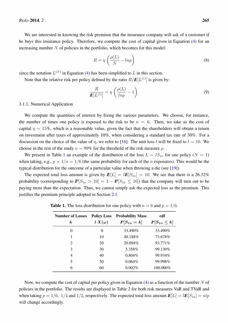
We present in Table 1 an example of the distribution of the loss L = lS1n for one policy (N = 1)when taking, e.g., p = 1/n = 1/6 (the same probability for each of the n exposures). This would be thetypical distribution for the outcome of a particular value when throwing a die (see [19]).

The expected total loss amount is given by IE[L] = lIE[S1n] = 10. We see that there is a 26.32%probability (corresponding to IP[S1n > 10] = 1 − IP[S1n ≤ 10]) that the company will turn out to bepaying more than the expectation. Thus, we cannot simply ask the expected loss as the premium. Thisjustifies the premium principle adopted in Section 2.1.

Table 1. The loss distribution for one policy with n = 6 and p = 1/6.

Number of Losses Policy Loss Probability Mass cdfk l X(ω) IP[S1n = k] IP[S1n ≤ k]

0 0 33.490% 33.490%1 10 40.188% 73.678%2 20 20.094% 93.771%3 30 5.358% 99.130%4 40 0.804% 99.934%5 50 0.064% 99.998%6 60 0.002% 100.000%

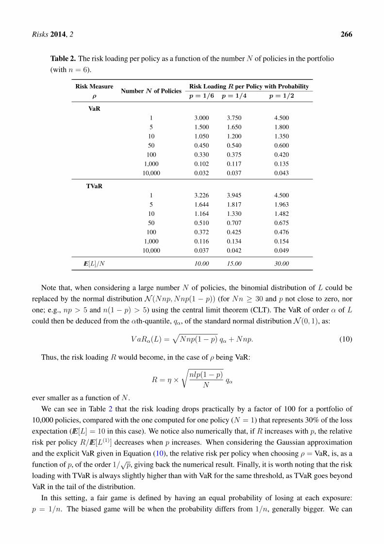
Now, we compute the cost of capital per policy given in Equation (4) as a function of the numberN ofpolicies in the portfolio. The results are displayed in Table 2 for both risk measures VaR and TVaR andwhen taking p = 1/6, 1/4 and 1/2, respectively. The expected total loss amount IE[L] = lIE[S1n] = nlp

will change accordingly.

Risks 2014, 2 266

Table 2. The risk loading per policy as a function of the numberN of policies in the portfolio(with n = 6).

Risk MeasureNumberN of Policies

Risk LoadingR per Policy with Probabilityρ p = 1/6 p = 1/4 p = 1/2

VaR1 3.000 3.750 4.5005 1.500 1.650 1.800

10 1.050 1.200 1.35050 0.450 0.540 0.600

100 0.330 0.375 0.4201,000 0.102 0.117 0.13510,000 0.032 0.037 0.043

TVaR1 3.226 3.945 4.5005 1.644 1.817 1.963

10 1.164 1.330 1.48250 0.510 0.707 0.675

100 0.372 0.425 0.4761,000 0.116 0.134 0.15410,000 0.037 0.042 0.049

IE[L]/N 10.00 15.00 30.00

Note that, when considering a large number N of policies, the binomial distribution of L could bereplaced by the normal distribution N (Nnp,Nnp(1 − p)) (for Nn ≥ 30 and p not close to zero, norone; e.g., np > 5 and n(1 − p) > 5) using the central limit theorem (CLT). The VaR of order α of Lcould then be deduced from the αth-quantile, qα, of the standard normal distribution N (0, 1), as:

V aRα(L) =√Nnp(1− p) qα +Nnp. (10)

Thus, the risk loading R would become, in the case of ρ being VaR:

R = η ×√nlp(1− p)

Nqα

ever smaller as a function of N .We can see in Table 2 that the risk loading drops practically by a factor of 100 for a portfolio of

10,000 policies, compared with the one computed for one policy (N = 1) that represents 30% of the lossexpectation (IE[L] = 10 in this case). We notice also numerically that, if R increases with p, the relativerisk per policy R/IE[L(1)] decreases when p increases. When considering the Gaussian approximationand the explicit VaR given in Equation (10), the relative risk per policy when choosing ρ = VaR, is, as afunction of p, of the order 1/

√p, giving back the numerical result. Finally, it is worth noting that the risk

loading with TVaR is always slightly higher than with VaR for the same threshold, as TVaR goes beyondVaR in the tail of the distribution.

In this setting, a fair game is defined by having an equal probability of losing at each exposure:p = 1/n. The biased game will be when the probability differs from 1/n, generally bigger. We can

Risks 2014, 2 267

thus define two states, one with a “normal” or equilibrium state (p = 1/n) and a “crisis” state with aprobability q >> p. In the next section, we will introduce this distinction.

3.2. Introducing a Structure of Dependence to Reveal a Systemic Risk

We propose two examples of models introducing a structure of dependence between the risks, in orderto explore the occurrence of a systemic risk and, as a consequence, the limits to diversification. We stillconsider the sequence (Xi, i = 1, . . . , Nn) to model the occurrence of the risk, with a given severity l,for N policies, but do not assume anymore that the Xis are iid

3.2.1. A Dependent Model, but Conditionally Independent

We assume that the occurrence of the risks Xis depends on another phenomenon, represented by anrv, say U . Depending on the intensity of the phenomenon, i.e., the values taken by U , a risk Xi hasmore or less chances to occur. Suppose that the dependence between the risks is totally captured by U .Consider, w.l.o.g., that U can take two possible values denoted by one and zero; U can then be modeledby a Bernoulli B(p), 0 < p << 1. The rv U will be identified with the occurrence of a state of systemicrisk. Therefore, p could mathematically take any value between zero and one, but we choose it here tobe very small, since we want to explore rare events. We still model the occurrence of the risks with aBernoulli, but with a parameter depending on U . Since U takes two possible values, the same holds forthe parameters of the Bernoulli distribution of the conditionally independent rvs Xi | U , namely:

(Xi | U = 1) ∼ B(q) and (Xi | U = 0) ∼ B(p).

We choose q >> p, so that whenever U occurs (i.e., U = 1), it has a big impact in the sense that thereis a higher chance of loss. We include this effect in order to have a systemic risk (non-diversifiable) inour portfolio.

Looking at the total amount of losses SNn, its distribution can then be written, for k ∈ IN, as:

IP(SNn = k) = IP [SNn = k | U = 1] IP(U = 1) + IP [SNn = k | U = 0] IP(U = 0)

= p IP [SNn = k | U = 1] + (1− p) IP [SNn = k | U = 0].

The conditional and independent variables, Sq := SNn| (U = 1) and Sp := SNn| (U = 0), are distributedas Binomials B(Nn, q) and B(Nn, p), with mass probability distributions denoted by fSq

and fSp,

respectively. The mass probability distribution fS of SNn appears as a mixture of fSqand fSp

(see,e.g., [20]):

fS = p fSq+ (1− p) fSp

with Sq ∼ B(Nn, q) and Sp ∼ B(Nn, p). (11)

Note that p = 0 gives back the normal state, developed in Section 3.1.The expected loss amount for the portfolio, denoting L = L(N), is given by:

IE[L] = l × IE[SNn] = l ×(p IE[Sq] + (1− p) IE[Sp]

)= Nnl

(p q + (1− p) p

)whereas for each policy, it is:

l

NIE[L] = l n

(p q + (1− p) p

)(12)

Risks 2014, 2 268

from which we deduce the risk loading defined in Equations (3) and (4).Let us evaluate the variance var(SNn) of SNn. Straightforward computations (see [19]) give:

IE[S2Nn] = Nn

[p q(1− q +Nnq

)+ (1− p) p

(1− p+Nnp

)]which, combined with Equation (12), provides:

var(SNn) = Nn[q(1− q)p+ p(1− p)(1− p) +Nn(q − p)2p(1− p)

]from which we deduce the variance for the loss of one contract as 1

N2 var(L) = l2

N2 var(SNn), i.e.,

1

N2var(L) =

l2n

N

(q(1− q)p+ p(1− p)(1− p)

)+ l2n2(q − p)2p(1− p). (13)

Notice that in the variance for one contract, the first term will decrease as the number of contractsincreases, but not the second one. It does not depend on N and, thus, represents the non-diversifiablepart of the risk.


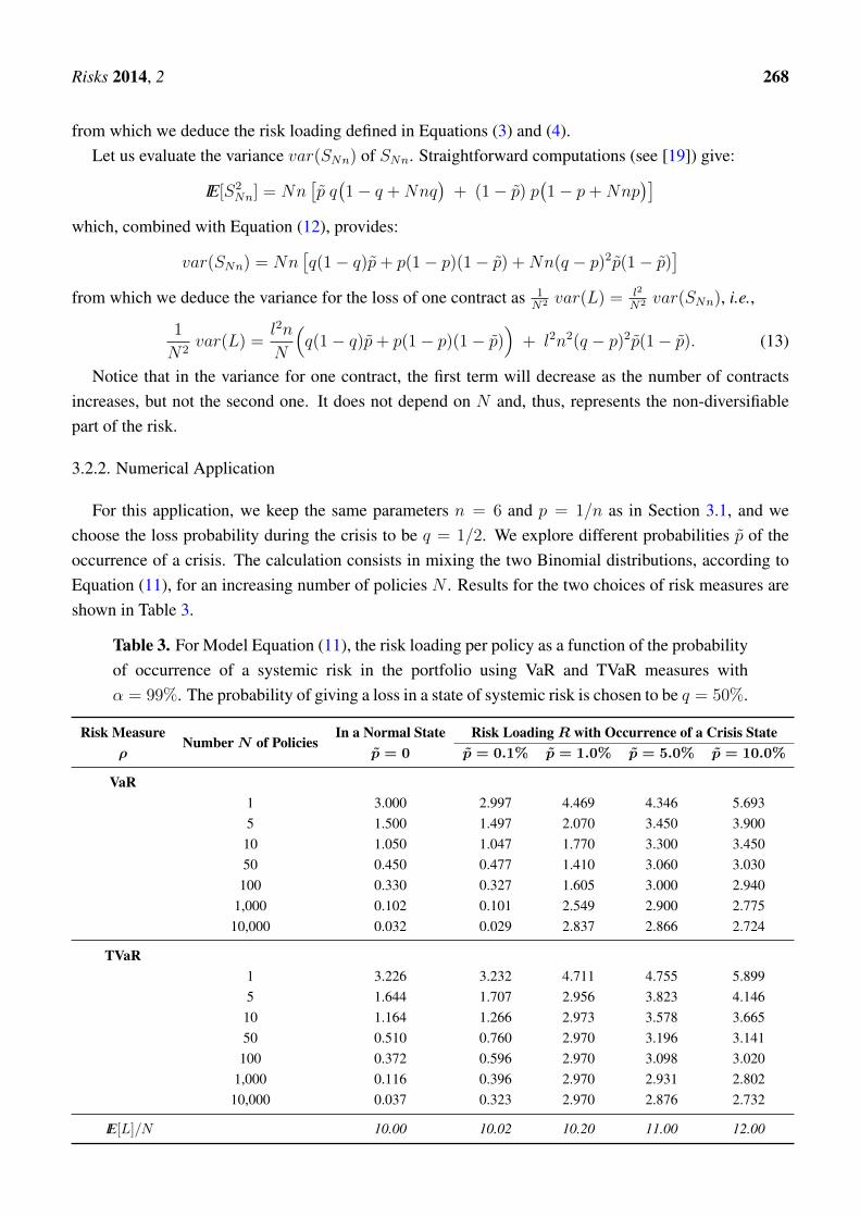
For this application, we keep the same parameters n = 6 and p = 1/n as in Section 3.1, and wechoose the loss probability during the crisis to be q = 1/2. We explore different probabilities p of theoccurrence of a crisis. The calculation consists in mixing the two Binomial distributions, according toEquation (11), for an increasing number of policies N . Results for the two choices of risk measures areshown in Table 3.

Table 3. For Model Equation (11), the risk loading per policy as a function of the probabilityof occurrence of a systemic risk in the portfolio using VaR and TVaR measures withα = 99%. The probability of giving a loss in a state of systemic risk is chosen to be q = 50%.


In a Normal State Risk LoadingR with Occurrence of a Crisis Stateρ p = 0 p = 0.1% p = 1.0% p = 5.0% p = 10.0%

VaR1 3.000 2.997 4.469 4.346 5.6935 1.500 1.497 2.070 3.450 3.90010 1.050 1.047 1.770 3.300 3.45050 0.450 0.477 1.410 3.060 3.030

100 0.330 0.327 1.605 3.000 2.9401,000 0.102 0.101 2.549 2.900 2.775

10,000 0.032 0.029 2.837 2.866 2.724

TVaR1 3.226 3.232 4.711 4.755 5.8995 1.644 1.707 2.956 3.823 4.146

10 1.164 1.266 2.973 3.578 3.66550 0.510 0.760 2.970 3.196 3.141100 0.372 0.596 2.970 3.098 3.020

1,000 0.116 0.396 2.970 2.931 2.80210,000 0.037 0.323 2.970 2.876 2.732

IE[L]/N 10.00 10.02 10.20 11.00 12.00

Risks 2014, 2 269

In Table 3, we see well the effect of the non-diversifiable risk. As expected, when the probability ofoccurrence of a crisis is high, the diversification does not play a significant role anymore, already with100 contracts in the portfolio. The interesting point is that for p ≥ 1%, the risk loading barely changeswhen there is a large number of policies (starting at N = 1,000) in the portfolio. This is true for bothVaR and TVaR. The non-diversifiable term dominates the risk. When looking at a lower probability pof the occurrence of a crisis, we notice that the choice of the risk measure matters. For instance, whenchoosing p = 0.1%, the risk loading, compared to the normal state, is multiplied by 10 in the case ofTVaR, for N = 10,000 policies, and hardly moves in the case of VaR! This effect remains, but to a lowerextent, when diminishing the number of policies. It is clear that the VaR measure does not capture thecrisis state well, while TVaR is sensitive to the change of state, even with such a small probability and ahigh number of policies.

Another interesting effect worth noticing is the fact that the risk loading for any given N shouldincrease with increasing p since the influence of the biased die should increase (as it appears clearlyin (12) and (13), the expectation and variance being increasing functions of p (with p < 1/2)). Yet,we see that, with VaR and TVaR, it is not the case starting with N = 50, although the effect is muchsmaller for TVaR. It seems to decrease when p increases from 5 to 10%. Pushing p to 15%, we seethat the effect of the bias levels off, which could explain the fluctuations around this level and thus thisnumerical instability.

To explore the increase of the risk loading of the VaR for p = 1%, we redid 1,000 times the 106

simulations. It turns out that the obtained values are very unstable, for instance for N = 10, 000, itjumps from 0.2 to 2.9, without taking any value in between. For the TVaR, it is more stable and we donot see such a behavior; in this case, the variation is less than 1%. When considering values for p closeto 1% (0.9 or 1.1%), the variation for the VaR becomes again more or less stable, we do not observe anymore such jumps.

3.2.3. A More Realistic Setting to Introduce a Systemic Risk

We adapt further the previous setting to a more realistic description of a crisis. At each of the nexposures to the risk, in a state of systemic risk, the entire portfolio will be touched by the same increasedprobability of loss, whereas, in a normal state, the entire portfolio will be subject to the same equilibriumprobability of loss.

For this modeling, it is more convenient to rewrite the sequence (Xi, i = 1, . . . , Nn) with a vectorialnotation, namely (Xj, j = 1, . . . , n), where the vector Xj is defined by Xj = (X1j, . . . , XNj)

T .Hence, the total loss amount SNn can be rewritten as:

SNn =n∑j=1

S(j) where S(j) is the sum of the components of Xj : S(j) =N∑i=1

Xij.

We keep the same notation for the Bernoulli rv U determining the state and for its parameter p.However, now, instead of defining a normal (U = 0) or a crisis (U = 1) state on each element of(Xi, i = 1, . . . , Nn), we do it on each vector Xj , 1 ≤ j ≤ n. It comes back to define a sequence of

Risks 2014, 2 270

iid rvs (Uj, j = 1, . . . , n) with parent rv U . Hence, we deduce that S(j) follows a Binomial distributionwhose probability depends on Uj:

S(j) | (Uj = 1) ∼ B(N, q) and S(j) | (Uj = 0) ∼ B(N, p).

Note that these conditional rvs are independent.Let us introduce the event Al defined, for l = 0, . . . , n, as:

Al := l vectors Xj are exposed to a crisis state and n−l to a normal state =( n∑j=1

Uj = l)

whose probability is given by IP(Al) = IP( n∑j=1

Uj = l)

=

(n

l

)pl (1− p)n−l.

We can then write that:

IP(SNn = k) =n∑l=0

IP(SNn = k | Al)IP(Al) =n∑l=0

(n

l

)pl (1− p)n−l IP

[S(l)q + S(n−l)

p = k]

(14)

with, by conditional independence,

S(l)q =

l∑j=1

(S(j) | Uj =1

)∼ B(Nl, q) and S(n−l)

p =n−l∑j=1

(S(j) | Uj =0

)∼ B(N(n− l), p). (15)

Expectation and variance are obtained by straightforward computations (see [19]). We have:

IE[SNn] = Nn((q − p

)p+ p

)(16)

and, for one contract,1

NIE[L] =

l

NIE[SNn] = nl (p q + (1− p) p)

which is equal to the expectation Equation (12) obtained with the previous method. The variance can bededuced from Equation (16) and:

IE[S2Nn] = Nn

(q(1− q)p+ p(1− p)(1− p)

)+ N2n2

(p(1− p) + qp

)2+N2n(q − p)2p(1− p)

hence:var(SNn) = Nn

[q(1− q)p+ p(1− p)(1− p) +N(q − p)2p(1− p)

]which is different from the variance var(SNn) obtained with the previous model in Section 3.2.1.

Now, for one contract, we obtain:

1

N2var(L) =

l2

N2var(SNn) =

l2n

N

(q(1− q)p+ p(1− p)(1− p)

)+ l2n (q − p)2p(1− p). (17)

Notice that the last term appearing in Equation (17) is only multiplied by n and not n2, as inEquation (13), and not diversifiable by the number N of policies. It looks like the one of Equation (13);however, its effect is smaller than in the previous model. With this method, we have also achievedproducing a process with a non-diversifiable risk.

Risks 2014, 2 271


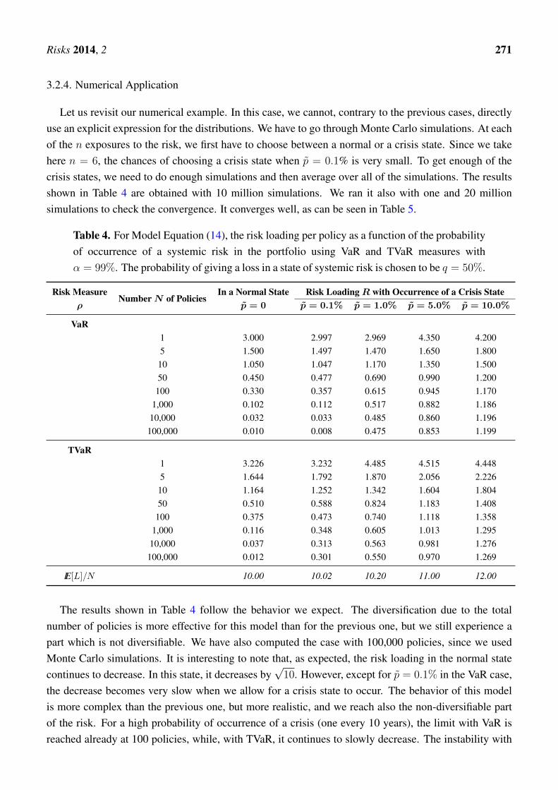
Let us revisit our numerical example. In this case, we cannot, contrary to the previous cases, directlyuse an explicit expression for the distributions. We have to go through Monte Carlo simulations. At eachof the n exposures to the risk, we first have to choose between a normal or a crisis state. Since we takehere n = 6, the chances of choosing a crisis state when p = 0.1% is very small. To get enough of thecrisis states, we need to do enough simulations and then average over all of the simulations. The resultsshown in Table 4 are obtained with 10 million simulations. We ran it also with one and 20 millionsimulations to check the convergence. It converges well, as can be seen in Table 5.

Table 4. For Model Equation (14), the risk loading per policy as a function of the probabilityof occurrence of a systemic risk in the portfolio using VaR and TVaR measures withα = 99%. The probability of giving a loss in a state of systemic risk is chosen to be q = 50%.



VaR1 3.000 2.997 2.969 4.350 4.2005 1.500 1.497 1.470 1.650 1.80010 1.050 1.047 1.170 1.350 1.50050 0.450 0.477 0.690 0.990 1.200

100 0.330 0.357 0.615 0.945 1.1701,000 0.102 0.112 0.517 0.882 1.186

10,000 0.032 0.033 0.485 0.860 1.196100,000 0.010 0.008 0.475 0.853 1.199

TVaR1 3.226 3.232 4.485 4.515 4.4485 1.644 1.792 1.870 2.056 2.226

10 1.164 1.252 1.342 1.604 1.80450 0.510 0.588 0.824 1.183 1.408100 0.375 0.473 0.740 1.118 1.358

1,000 0.116 0.348 0.605 1.013 1.29510,000 0.037 0.313 0.563 0.981 1.276100,000 0.012 0.301 0.550 0.970 1.269

IE[L]/N 10.00 10.02 10.20 11.00 12.00

The results shown in Table 4 follow the behavior we expect. The diversification due to the totalnumber of policies is more effective for this model than for the previous one, but we still experience apart which is not diversifiable. We have also computed the case with 100,000 policies, since we usedMonte Carlo simulations. It is interesting to note that, as expected, the risk loading in the normal statecontinues to decrease. In this state, it decreases by

√10. However, except for p = 0.1% in the VaR case,

the decrease becomes very slow when we allow for a crisis state to occur. The behavior of this modelis more complex than the previous one, but more realistic, and we reach also the non-diversifiable partof the risk. For a high probability of occurrence of a crisis (one every 10 years), the limit with VaR isreached already at 100 policies, while, with TVaR, it continues to slowly decrease. The instability with

Risks 2014, 2 272

increasing p that we noticed in Table 3 has disappeared here for both VaR and TVaR. The cost of capitalalways increases with increasing p, except for N = 1. This could be due to the fact that we consideronly one discrete rv and/or to the numerical stability of the results.

Concerning the choice of risk measure, we see a similar behavior as in Table 3 for the caseN = 10,000 and p = 0.1%: VaR is unable to catch the possible occurrence of a crisis state, which showsits limitation as a risk measure. Although we know that there is a part of the risk that is non-diversifiable,VaR does not catch it really when N = 10,000 or 100,000, while TVaR does not decrease significantlybetween 10,000 and 100,000 reflecting the fact that the risk cannot be completely diversified away.

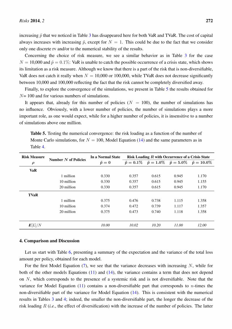
Finally, to explore the convergence of the simulations, we present in Table 5 the results obtained forN= 100 and for various numbers of simulations.

It appears that, already for this number of policies (N = 100), the number of simulations hasno influence. Obviously, with a lower number of policies, the number of simulations plays a moreimportant role, as one would expect, while for a higher number of policies, it is insensitive to a numberof simulations above one million.

Table 5. Testing the numerical convergence: the risk loading as a function of the number ofMonte Carlo simulations, for N = 100, Model Equation (14) and the same parameters as inTable 4.



VaR1 million 0.330 0.357 0.615 0.945 1.170

10 million 0.330 0.357 0.615 0.945 1.15520 million 0.330 0.357 0.615 0.945 1.170

TVaR1 million 0.375 0.476 0.738 1.115 1.358

10 million 0.374 0.472 0.739 1.117 1.35720 million 0.375 0.473 0.740 1.118 1.358

IE[L]/N 10.00 10.02 10.20 11.00 12.00

4. Comparison and Discussion

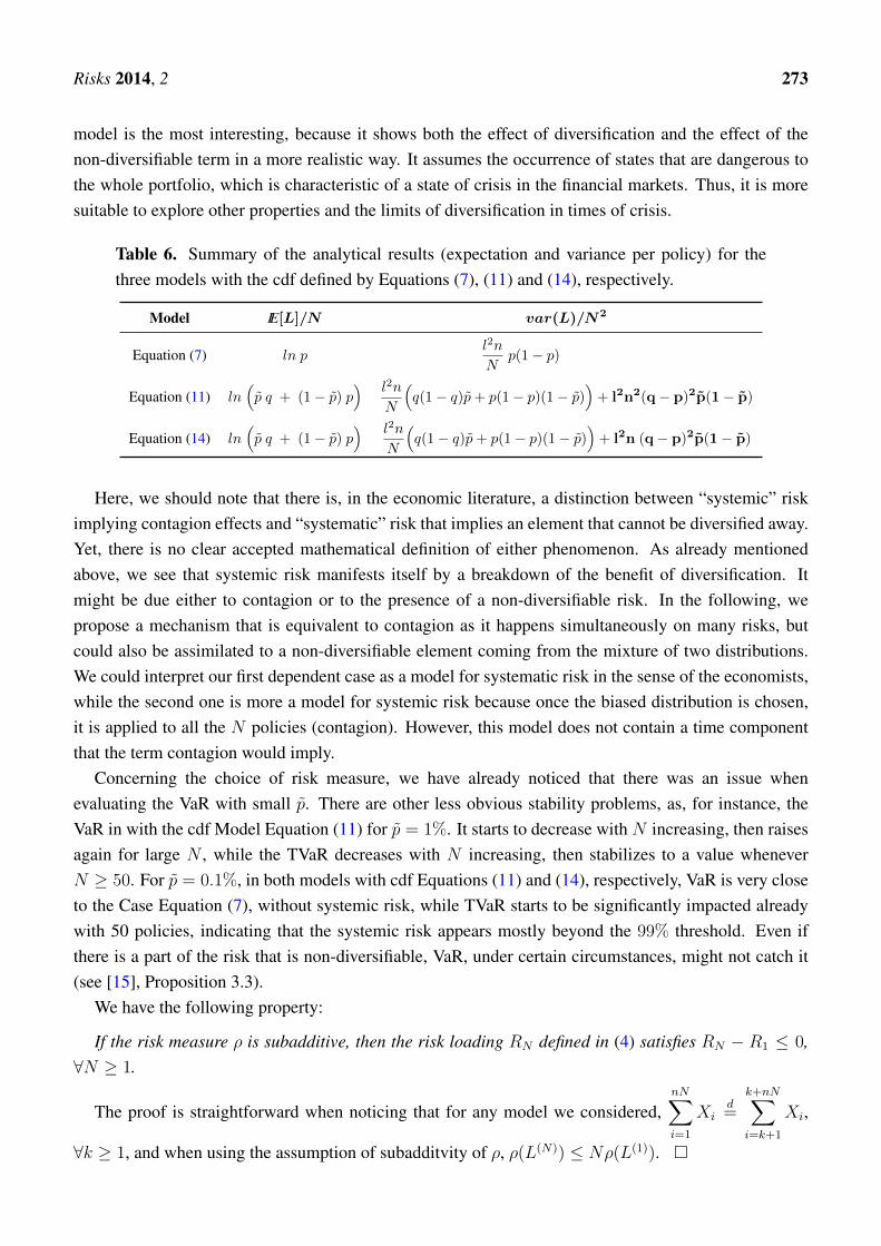
Let us start with Table 6, presenting a summary of the expectation and the variance of the total lossamount per policy, obtained for each model.

For the first Model Equation (7), we see that the variance decreases with increasing N , while forboth of the other models Equations (11) and (14), the variance contains a term that does not dependon N , which corresponds to the presence of a systemic risk and is not diversifiable. Note that thevariance for Model Equation (11) contains a non-diversifiable part that corresponds to n-times thenon-diversifiable part of the variance for Model Equation (14). This is consistent with the numericalresults in Tables 3 and 4; indeed, the smaller the non-diversifiable part, the longer the decrease of therisk loading R (i.e., the effect of diversification) with the increase of the number of policies. The latter

Risks 2014, 2 273

model is the most interesting, because it shows both the effect of diversification and the effect of thenon-diversifiable term in a more realistic way. It assumes the occurrence of states that are dangerous tothe whole portfolio, which is characteristic of a state of crisis in the financial markets. Thus, it is moresuitable to explore other properties and the limits of diversification in times of crisis.

Table 6. Summary of the analytical results (expectation and variance per policy) for thethree models with the cdf defined by Equations (7), (11) and (14), respectively.

Model IE[L]/N var(L)/N2

Equation (7) ln pl2n

Np(1− p)

Equation (11) ln(p q + (1− p) p

) l2n

N

(q(1− q)p+ p(1− p)(1− p)

)+ l2n2(q− p)2p(1− p)

Equation (14) ln(p q + (1− p) p

) l2n

N

(q(1− q)p+ p(1− p)(1− p)

)+ l2n (q− p)2p(1− p)

Here, we should note that there is, in the economic literature, a distinction between “systemic” riskimplying contagion effects and “systematic” risk that implies an element that cannot be diversified away.Yet, there is no clear accepted mathematical definition of either phenomenon. As already mentionedabove, we see that systemic risk manifests itself by a breakdown of the benefit of diversification. Itmight be due either to contagion or to the presence of a non-diversifiable risk. In the following, wepropose a mechanism that is equivalent to contagion as it happens simultaneously on many risks, butcould also be assimilated to a non-diversifiable element coming from the mixture of two distributions.We could interpret our first dependent case as a model for systematic risk in the sense of the economists,while the second one is more a model for systemic risk because once the biased distribution is chosen,it is applied to all the N policies (contagion). However, this model does not contain a time componentthat the term contagion would imply.

Concerning the choice of risk measure, we have already noticed that there was an issue whenevaluating the VaR with small p. There are other less obvious stability problems, as, for instance, theVaR in with the cdf Model Equation (11) for p = 1%. It starts to decrease with N increasing, then raisesagain for large N , while the TVaR decreases with N increasing, then stabilizes to a value wheneverN ≥ 50. For p = 0.1%, in both models with cdf Equations (11) and (14), respectively, VaR is very closeto the Case Equation (7), without systemic risk, while TVaR starts to be significantly impacted alreadywith 50 policies, indicating that the systemic risk appears mostly beyond the 99% threshold. Even ifthere is a part of the risk that is non-diversifiable, VaR, under certain circumstances, might not catch it(see [15], Proposition 3.3).

We have the following property:

If the risk measure ρ is subadditive, then the risk loading RN defined in (4) satisfies RN − R1 ≤ 0,∀N ≥ 1.

The proof is straightforward when noticing that for any model we considered,nN∑i=1

Xid=

k+nN∑i=k+1

Xi,

∀k ≥ 1, and when using the assumption of subadditvity of ρ, ρ(L(N)) ≤ Nρ(L(1)).

Risks 2014, 2 274

This property is satisfied in the three cases. We also see that RN is a decreasing function of N forTVaR in all tables, but not for VaR. For the latter, we see, in the first dependence model, an increase ofVaR for p = 1% fromN = 100 onwards and, in the second case, for p = 10% fromN = 1′000 onwards.The reason for this increase could be due to numerical instabilities or to a break of subadditivity of VaR.

5. Conclusions

In this study, we have shown the effect of diversification on the pricing of insurance risk through thefirst simple modeling. Then, for understanding and analyzing possible limitations to diversificationbenefits, we propose two alternative stochastic models, introducing dependence between risks byassuming the existence of an underlying systemic risk. These models, defined with mixing distributions,allow for a straightforward analytical evaluation of the impact of the non-diversifiable part, whichappears in the close form expression of the variance. We have purposely adopted here a probabilisticapproach for modeling the dependence and the existence of systemic risk. It could be easily generalizedto a time series interpretation by assigning a time step to each exposure n. In the last model, theoccurrence of the rv U = 1 could then be identified with the time of crisis.

In real life, insurers have to pay special attention to the effects that can weaken the diversificationbenefits. For instance, in the case of motor insurance, the appearance of a hail storm will introduce a“bias” in the usual risk of accidents, due to a cause independent of the car drivers, which will hit a bignumber of cars at the same time and, thus, cannot be diversified among the various policies. There areother examples, in life insurance, for instance, with a pandemic or mortality trend that would affect theentire portfolio and that cannot be diversified away. Special care must be given to those risks, as they willaffect greatly the risk loading of the premium, as can be seen in our examples. These examples mightalso find applications for real cases. This approach can be generalized to investments and banking; bothare subject to systemic risk, although of a different nature than in the above insurance examples.

The last model we suggested, introducing the occurrence of crisis, may find an interesting applicationfor investment and the change in the risk appetite of investors. It will be the subject of a following paper.Moreover, the models we introduce here allow one to point out explicitly the impact of dependence;they are simple enough to compute an analytic expression and to analyze the impact of the emergence ofsystemic risks. Yet, they are formulated in such a way that extensions to more sophisticated models areeasy and clear. In particular, it makes it possible to obtain an extension to non-identically-distributed rvsor when considering random severity. Another interesting perspective would be to consider econometricmodels with multiple states.

Acknowledgements

Partial support from RARE-318984 (an FP7 Marie Curie IRSES Fellowship) is kindly acknowledged.

Author Contributions

All authors contributed equally to this work.

Risks 2014, 2 275

Conflicts of Interest

The authors declare no conflicts of interest.

References

1. Caballero, R.J.; Kurlat, P. The ‘Surprising’ Origin and Nature of Financial Crises:A Macroeconomic Policy Proposal. In Financial Stability and Macroeconomic Policy,Federal Reserve Bank of Kansas City 2009. Available online: http://papers.ssrn.com/sol3/papers.cfm?abstract_id=1473918 (accessed on 17 November 2009).

2. Cont, R.; Moussa, A.; Santos, E. Network structure and systemic risk in banking systems. InHandbook of Systemic Risk; Fouque, L., Ed.; Cambridge University Press: Cambridge, UK, 2013.

3. Acharya, V.V.; Pedersen, L.H.; Philippon, T.; Richardson, M. Measuring Systemic Risk.Preprint, 2010. Available online: http://pages.stern.nyu.edu/ sternfin/vacharya/public_html/MeasuringSystemicRisk_final.pdf (accessed on 24 March 2014).

4. Brunnermeier, M.K.; Cheridito, P. Measuring and allocating systemic risk. Working Paper, 2013.Available online: http://papers.ssrn.com/sol3/papers.cfm?abstract_id=2372472 (accessed on 24March 2014).

5. Brunnermeier, M.K.; Sannikov, Y. A Macroeconomic Model with a Financial Sector.Working Paper, 2013. Available online: http://papers.ssrn.com/sol3/papers.cfm?abstract_id=2160894 (accessed on 24 March 2014).

6. He, Z.; Krishnamurthy, A. A Macroeconomic Framework for Quantifying Systemic Risk.Chicago Booth Paper No. 12-37, 2014. Available online: http://papers.ssrn.com/sol3/papers.cfm?abstract_id=2133412 (accessed on 24 March 2014).

7. Martinez-Miera, D.; Suarez, J. A Macroeconomic Model of Endogenous SystemicRisk Taking. Working Paper, 2012. Available online: http://papers.ssrn.com/sol3/papers.cfm?abstract_id=2153575 (accessed on 24 March 2014).

8. Billio, M.; Getmansky, M.; Lo, A.W.; Pelizzon, L. Economic Measures of the Systemic Risk in theFinance and Insurance Sectors. NBER Working Paper Series no. 16223, 2010. Available online:http://www.nber.org/papers/w16223 (accessed on 24 March 2014).

9. Bisias, D.; Flood, M.; Lo, A.W.; Valavanis, S. A survey of systemic risk analytics.Office of Financial Research Working Paper, 2012. Available online: http://papers.ssrn.com/sol3/papers.cfm?abstract_id=1983602 (accessed on 24 March 2014).

10. Brownlees, C.T.; Engle, R. Volatility, Correlation and Tails for Systemic RiskMeasurement. Working Paper, 2012. Available online: http://papers.ssrn.com/sol3/papers.cfm?abstract_id=1611229 (accessed on 24 March 2014).

11. Duffie, D. Systemic Risk Exposures: A 10 by 10 by 10 Approach, NBER Working Paper No.17281, 2011. Available online: http://www.nber.org/papers/w17281 (accessed on 24 March 2014).

12. Giglio, S.; Kelly, B.; Pruitt, S. Systemic Risk and the Macroeconomy: An EmpiricalEvaluation. Chicago Booth Paper No. 12-49, 2013. Available online: http://papers.ssrn.com/sol3/papers.cfm?abstract_id=2158347 (accessed on 24 March 2014).

Risks 2014, 2 276

13. Bürgi, R.; Dacorogna, M.; Iles, R. Risk Aggregation, dependence structure and diversificationbenefit. In Stress testing for financial institutions; Rösch, D., Scheule, H. Eds.; Incisive Media:London, UK, 2008.

14. Emmer, S.; Kratz, M.; Tasche, D. What Is the Best Risk Measure in Practice? A Comparison ofStandard Measures. ArXiV pre-print arXiv:1312.1645, 2013. Available online: http://arxiv.org/abs/1312.1645 (accessed on 24 March 2014).

15. Emmer, S; Tasche, D. Calculating Credit Risk Capital Charges with the One-factor Model. J. Risk2004, 7, 85–103.

16. Dacorogna, M.M.; Hummel, C. Alea jacta est, an illustrative example of pricing risk. SCORTechnical Newsletter; SCOR Global P&C: Zurich, Switzerland, 2008; pp. 1–4.

17. McNeil, A.; Frey, R; Embrechts, P. Quantitative Risk Management; Princeton University Press:Princeton, NJ, USA, 2005.

18. Artzner, P.; Delbaen, F.; Eber, J.-M.; Heath, D. Coherent measures of risks. Math. Financ. 1999, 9,203–228.

19. Busse, M.; Dacorogna, M.; Kratz, M. Does risk diversification always work? The answer throughsimple modeling. SCOR Pap. 2013, 24, 1–19.

20. Everitt, B.S.; Hand, D.J. Finite Mixture Distributions; Chapman & Hall: London, UK, 1981.

c© 2014 by the authors; licensee MDPI, Basel, Switzerland. This article is an open access articledistributed under the terms and conditions of the Creative Commons Attribution license(http://creativecommons.org/licenses/by/3.0/).

the impact of systemic risk on the diversification benefits of a risk portfolio

Documents