103

Tijdschrift voor Economie en ManagementVol. L, 1, 2005

Optimal Portfolio Selection for Cash-Flowswith Bounded Capital at Risk

by D. VYNCKE, M. GOOVAERTS, J. DHAENE and S. VANDUFFEL

Marc GoovaertsKULeuven, AFI Actuarial Science, Leuven and University of Amsterdam, The Netherlands

David VynckeKULeuven, AFI Actuarial Science, Leuven

Steven Van DuffelKULeuven, AFI Actuarial Science, Leuven

Jan DhaeneKULeuven, AFI Actuarial Science, Leuven and University of Amsterdam, The Netherlands

ABSTRACT

We consider a continuous-time Markowitz type portfolio problem that consists of minimizing the discounted cost of a given cash-fl ow under the constraint of a restricted Capital at Risk. In a Black-Scholes setting, upper and lower bounds are obtained by means of simple analytical expressions that avoid the classical simulation approach for this type of problems. The problem is easily extended to cope with more general discount processes.

Keywords: Black-Scholes model, Capital at Risk, portfolio optimization, Value at Risk.

* The authors would like to acknowledge the fi nancial support of the Onderzoeksfonds K.U. Leuven (GOA/02: Actuariële, fi nanciële en statistische aspecten van afhankelijk-heden in verzekerings- en fi nanciële portefeuilles).

104

I. INTRODUCTION

The portfolio selection algorithm as introduced in Markowitz (1959) uses a mean-variance analysis to fi nd optimal portfolios. In this meth-od, a portfolio is called optimal if it yields the largest return among all portfolios with the same variance or, vice versa, if it has the smallest variance among all portfolios with the same return. For long term in-vestments, however, the use of the variance as a risk measure leads to a smaller proportion of risky assets in a portfolio than one would expect. Based on the empirical observation that stock indices are growing faster than riskless rates in the long run, the proportion of risky assets should increase with the duration of the investment period. But since the variance increases with time, the proportion of risky assets will decrease. Therefore, Emmer et al (2001) propose to use the Capital at Risk (CaR) as an alternative risk measure and derive a closed-form formula to calculate the optimal CaR-constrained portfolio.

The Capital at Risk of a portfolio is commonly defi ned as the differ-ence between the mean of the profi t-loss distribution and a small quan-tile of this distribution (the so-called Value at Risk), but Emmer et al (2001) use a different defi nition which limits the possibility of excess losses over the riskless investment. We will also follow this approach and show how optimal CaR-constrained portfolios can be obtained for cash-fl ows in a Black-Scholes setting.

In a Black-Scholes market the stock prices { S i (t)}

t � 0 for i = 1, …, d, evolve from the following equations:

d S i (t) = S

i (t) ( m i dt + ∑

j=1

d

s ij d W

j (t) ) , S i (0) = s

i , i = 1, …, d

where W(t) is a standard d-dimensional Brownian motion, m = (m1, …,

md)' is the vector of stock-appreciation rates, and s = ( s

ij ) 1�i, j�d is the matrix of stock-volatilities.

Denoting the fraction of the wealth X(p, t) that is invested in as-set i by p

i(t), the wealth process of an initial unit amount follows the

dynamic

dX(p, t) = X(p, t) (p'mdt + p'sdW(t)), X(p, 0) = 1. (1)

As in Emmer et al (2001), we assume that the fractions in the dif-ferent stocks remain constant on [0, T], i.e. p(t) = p = (p

1, …, p

d)'. So,

105

since the stock prices evolve randomly, one has to follow a dynamic trading strategy to keep the fractions of wealth invested in the different stocks constant. Solving the SDE (1) yields

X(p, t) = exp {Y(p, t)} (2)

where Y(p, t) equals

Y(p, t) = p'mt – p's2p t __ 2 + p'sW(t). (3)

In the following section we extend some results obtained by Em-mer et al (2001) to an actuarial context where consecutive payments have to be made. But implementing the mean-CaR criterion in a multi-period model inevitably turns the portfolio selection problem into a very complex problem for which no analytical solutions exist. Con-sequently, this type of portfolio selection problem is generally tackled by means of simulation of the corresponding stochastic processes. In section III we construct close approximations to the model in order to avoid this excessive time-consuming approach. Section IV concludes with a numerical illustration of the approximations.

II. EXTENSION TO CASH-FLOWS

In an insurance setting, at certain points in time an amount is with-drawn from or added to the money invested. We consider a cash-fl ow c

t denoting the total payments for each year t (e.g. pensions in a pen-

sion fund). Throughout the paper we will assume that ct � 0 (t = 1,

…, T).

The present value of the cash-fl ow equals

V = ∑ t=1

T

c t e –Y(p, t) . (4)

with expected value given by

V0 = E[V] = ∑

t=1

T

c t e –m(p)t + s 2 (p)t (5)

where m(p) = p'm and s2(p) = p's2p. Obviously, we want to select a portfolio that minimizes V

0. Note however that there are restrictions

106

on the amounts of risky stocks that can be bought, due to the require-ments of control authorities. In addition, also due to regulators, the probability of “ruin” has to be restricted. Let e denote the maximum probability of “ruin allowed’’. Denoting the 1 – e quantile of the dis-counted cash-fl ow by Qe(p), i.e.

Pr [ ∑ t=1

T

c t e –Y(p, t) � Qe(p) ] = 1 – e (6)

we defi ne the Capital at Risk as

CaR = Qe(p) – ∑ t=1

T

c t e –rt (7)

where r is a constant reference interest rate, e.g. the riskless interest rate.

So, if we assume that the provision for the future payment obliga-tions is the 1 – e quantile, then the CAR is the required provision in excess of the required provision in case of riskless investments.By taking into account the extra cost of the CaR, we come to the fol-lowing optimization problem:

min p V

0 + u(CaR), subject to p j � 0, ∑

j=1

d

p j = 1 , CaR � C

where the increasing function u(·) denotes the supplementary cost of the Capital at Risk and where C denotes the maximum CaR al-lowed.

Since the quantile Qe(p) is very hard (or even impossible) to obtain due to the dependency structure between the random variables Y(p, t), t = 1, …, T, in (4), it seems impossible to solve this optimization prob-lem without using Monte Carlo simulation. In the next section, we will show how this excessive time-consuming approach can be avoided by using easily computable approximations to Qe(p).

107

III. AVOIDING SIMULATION

Instead of calculating the exact quantile of the distribution, we will look for bounds, in the sense of “more favourable/less dangerous’’ and “less favourable/more dangerous’’, with a simpler structure. This technique is common practice in the actuarial literature. When lower and upper bounds are close to each other, together they can provide reliable information about the original and more complex variable. The notion “less favourable’’ or “more dangerous’’ will be defi ned by means of the convex order.

Defi nition 1 A random variable V is smaller than a random variable W in convex order if

E [u(V)] � E [u(W)], (8)

for all convex functions u: ˙ " ˙ : x 7 u(x), provided the expectations exist. This is denoted as

V �cx

W. (9)

Since convex functions are functions that take on their largest val-ues in the tails, the variable W is more likely to take on extreme values than the variable V, and thus W is more dangerous.

In Vyncke et al (2001) and Kaas et al (2001) upper and lower bounds for present value functions are constructed. These bounds in convex order turn out to be rather close to the exact present value distribution.

Proposition 1 Consider a sum of random variables

V = X1 + X

2 + … + X

n,

and defi ne the related stochastic quantities

Vu = F

X 1 –1 (U) + F

X 2 –1 (U) + … + F

X n –1 (U) (10)

Vl = E[X

1|Z] + E[X

2|Z] + … + E[X

n|Z], (11)

108

where U is a random variable, uniformly distributed on [0,1], and where Z can be any random variable for which the expectations exist. The following relations then hold:

Vl �

cx V �

cx V

u.

Proof: see Vyncke et al (2001) and Dhaene et al (2002).

It is clear that the lower bound Vl will perform at best if Z and V are

very similar, so we choose

Z = ∑ t=1

T

c t e –p'mt Y(p, t) (12)

which can be seen to be a fi rst order approximation of V.

For the (1 – ε)-quantiles of Vu and V

l we fi nd

Q e * (p) =

∑ t=1

T

c t exp { –m(p)t + r(p, t) s(p) √

_ t F –1 (1 – e) + ( 1 –

r 2 (p, t) ______ 2 ) s 2 (p)t }

(13)

with m(p) = p'm, s2(p) = p's2p and where the parameters r(p, t) are given by

r(p, t) = Corr(Y(p, t), Z) = ∑

i=1 t

b i _______

√______

t ∑i=1

T b

i 2 , with b

i = ∑ t=i

T

c t e –m(p)t

in case of the lower bound Vl, and r(p, t) � 1 in case of the upper

bound Vu. Note that r(p, t) depends on p only through m(p). Since

0 � r(p, t) � 1 and s(p) � 0, the quantile Q e * (p) is an increasing func-

tion of s(p). This implies that the adjusted Capital at Risk

CaR * = Q e * (p) – ∑

t=1

T

c t e –rt (14)

is also increasing in s(p) for both approximations. Note, however, that the adjusted CaR isn’t necessarily increasing with the planning

109

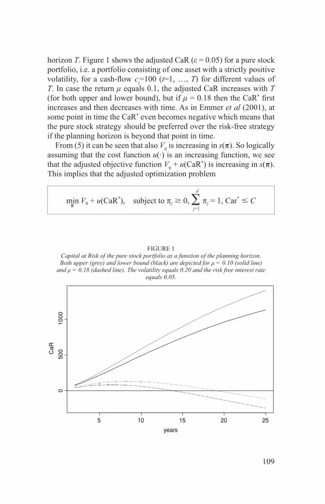
horizon T. Figure 1 shows the adjusted CaR (e = 0.05) for a pure stock portfolio, i.e. a portfolio consisting of one asset with a strictly positive volatility, for a cash-fl ow c

t=100 (t=1, …, T) for different values of

T. In case the return m equals 0.1, the adjusted CaR increases with T (for both upper and lower bound), but if m = 0.18 then the CaR* fi rst increases and then decreases with time. As in Emmer et al (2001), at some point in time the CaR* even becomes negative which means that the pure stock strategy should be preferred over the risk-free strategy if the planning horizon is beyond that point in time.

From (5) it can be seen that also V0 is increasing in s(p). So logically

assuming that the cost function u(·) is an increasing function, we see that the adjusted objective function V

0 + u(CaR*) is increasing in s(p).

This implies that the adjusted optimization problem

min p V

0 + u( CaR * ), subject to p j � 0, ∑

j=1

d

p j = 1 , Car * � C

years

CaR

5 10 15 20 25

050

010

00

FIGURE 1Capital at Risk of the pure stock portfolio as a funstion of the planning horizon. Both upper (grey) and lower bound (black) are depicted for m = 0.10 (solid line)

and m = 0.18 (dashed line). The volatility equals 0.20 and the risk free interest rate equals 0.05.

110

can be solved by minimizing s2(p) for each m(p) = m, and choosing the solution which minimizes the adjusted objective function. So, solving this optimization problem boils down to successively solving a quadratic program. Because of the specifi c nature of the optimization problem, the solution will also be part of the mean-variance effi cient frontier.

IV. NUMERICAL ILLUSTRATION

In this section we illustrate the method by considering a portfolio con-sisting of 5 risky stocks and 1 riskless bond. The stock-appreciation rates m and stock-volatilities s are given by

stock 1 2 3 4 5

m 0.1346 0.1659 0.1895 0.2014 0.095

s 0.1585 0.2293 0.3368 0.4299 0.0686

and their correlation matrix equals

( 1

0.7217

0.2571

-0.0719 0.408

0.7217

1 0.1436

-0.083 0.1419

0.2571

0.1436 1

0.0255 -0.0829

-0.0719

-0.083 0.0255

1 -0.1154

0.408

0.1419 -0.0829

-0.1154 1 )

The riskless bond yields a 0.05 return and we assume that the cost function is given by

u(x) = { 0.2x 0.05x x � 0 x � 0

This can be interpreted as follows: the insurance company has to pay a dividend of 20% to its shareholders if the CaR is positive and earns 5% (the risk-free interest rate) if the CaR is negative.

First, we consider a cash-fl ow ct = 100 (t=1, …, 20). For e = 0.05,

the proportions (in %) based on the upper bound Vu are very close to

those based on Vl, as can be seen from the following table. Note that p

0

indicates the proportion that is invested in the riskless bond.

111

appr.e

Vu

0.05V

l

0.05V

u

0.01V

l

0.01

p0

0.00 0.00 0.00 0.00

p1

0.00 0.00 0.00 0.00

p2

48.28 48.01 37.28 45.59

p3

27.16 27.30 20.44 24.35

p4

24.57 24.70 18.39 21.97

p5

0.00 0.00 23.90 8.10

m 18.10 18.11 16.03 17.37

s 18.23 18.25 13.90 16.67

V0

595.13 595.10 621.03 602.11

CaR* -139.10 -235.56 52.46 -0.12

cost 588.17 583.33 631.52 602.10

In Figure 2 the optimal portfolios based on Vu and V

l are indicated by

a circle and a rectangle respectively. For e = 0.01, the proportions ap-pear to be less effi cient for this kind of cash-fl ow (see also Figure 3).

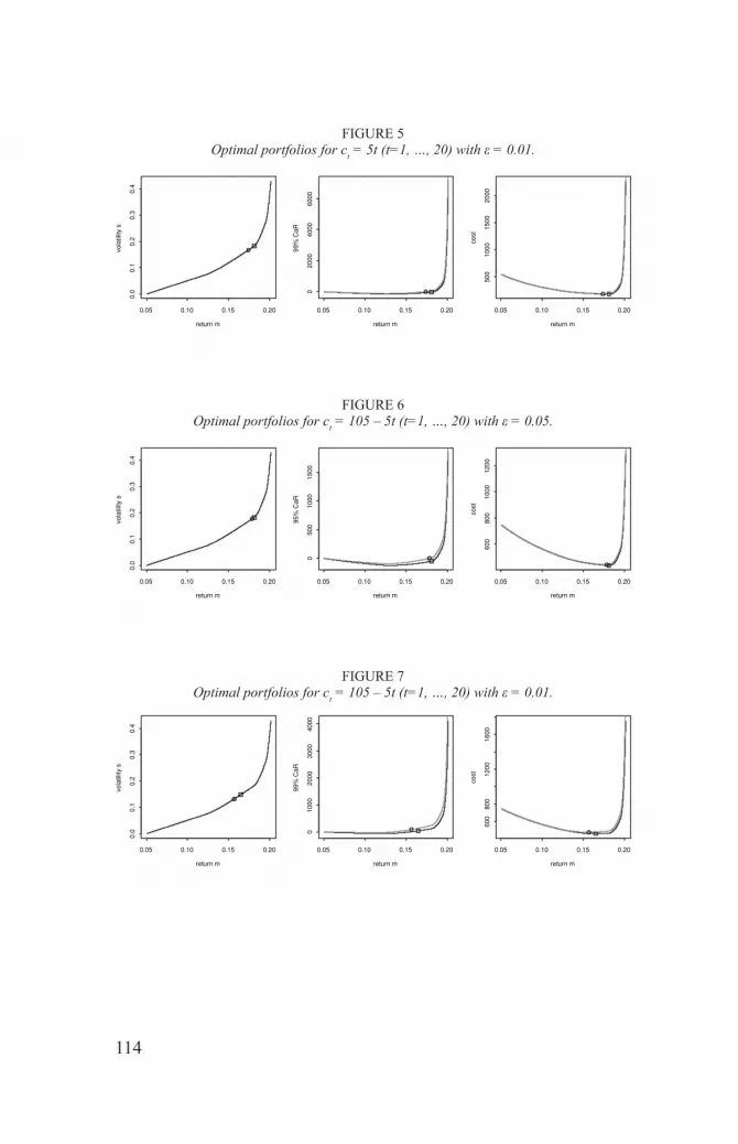
Next, we consider an increasing cash-fl ow ct = 5t (t=1, …, 20).

Apart from rounding errors, we see that the proportions for the Vu ap-

proximation equal those of the Vl approximation in case of e = 0.05.

For e = 0.01, the largest difference in proportion is approximately 8% (see also Figures 4 and 5).

appr.e

Vu

0.05V

l

0.05V

u

0.01V

l

0.01

p0

0.00 0.00 0.00 0.00

p1

0.00 0.00 0.00 0.00

p2

48.01 48.01 45.73 48.28

p3

27.30 27.30 24.42 27.16

p4

24.70 24.70 22.04 24.57

π5

0.00 0.00 7.82 0.00

m 18.11 18.11 17.39 18.10

s 18.25 18.25 16.72 18.23

V0

183.89 183.89 187.21 183.91

CaR* -155.02 -184.89 -0.19 -32.75

cost 176.14 174.67 187.20 182.27

112

Finally, we consider a decreasing cash-fl ow ct = 105-5t (t=1, …, 20).

For e = 0.05 (see Figure 6) as well as for e = 0.01 (see Figure 7), the method appears to perform quite well.

appr.e

Vu

0.05V

l

0.05V

u

0.01V

l

0.01

p0

0.00 0.00 0.00 0.00

p1

0.00 0.00 0.00 0.00

p2

48.52 48.28 34.96 40.04

p3

25.73 27.16 19.35 21.74

p4

23.24 24.57 17.40 19.59

p5

2.52 0.00 28.30 18.64

m 17.84 18.10 15.66 16.48

s 17.67 18.23 13.15 14.81

V0

442.18 440.98 459.03 451.36

CaR* 0.61 -51.86 91.55 43.59

cost 442.30 438.38 477.34 460.08

REFERENCES

Dhaene J., Denuit M., Goovaerts M.J., Kaas R. & Vyncke D., 2002, The Concept of Comonotonicity in Actuarial Science and Finance: Theory, Insurance: Mathematics and Economics, to appear.

Emmer S., Klüppelberg C., Korn R., 2001. Optimal Portfolios with Bounded Capital at Risk, Mathematical Finance 11, 4, 365-384.

Kaas R., Dhaene J., Goovaerts M.J., 2000. Upper and Lower Bounds for Sums of Random Variables, Insurance: Mathematics and Economics 27, 151-168.

Markowitz H., 1959. Portfolio Selection: Effi cient Diversifi cation of Investments (John Wiley & Sons, New York).

Vyncke D., Goovaerts M. & Dhaene J., 2001. Convex Upper and Lower Bounds for Present Value Functions, Applied Stochastic Models for Business and Industry, 17, 149-164.

113

return m

vola

tility

s

0.05 0.10 0.15 0.20

0.0

0.1

0.2

0.3

0.4

return m

95%

CaR

0.05 0.10 0.15 0.200

1000

2000

3000

4000

return m

cost

0.05 0.10 0.15 0.20

1000

1500

2000

2500

FIGURE 2Optimal portfolios for c

t =100 (t=1, …, 20) with e = 0.05.

return m

vola

tility

s

0.05 0.10 0.15 0.20

0.0

0.1

0.2

0.3

0.4

return m

99%

CaR

0.05 0.10 0.15 0.20

020

0040

0060

0080

00

return m

cost

0.05 0.10 0.15 0.20

500

1500

2500

3500

FIGURE 3Optimal portfolios for c

t =100 (t=1, …, 20) with e = 0.01.

return m

vola

tility

s

0.05 0.10 0.15 0.20

0.0

0.1

0.2

0.3

0.4

return m

95%

CaR

0.05 0.10 0.15 0.20

050

010

0015

0020

0025

00

return m

cost

0.05 0.10 0.15 0.20

200

400

600

800

1000

FIGURE 4Optimal portfolios for c

t = 5t (t=1, …, 20) with e = 0.05.

114

return m

vola

tility

s

0.05 0.10 0.15 0.20

0.0

0.1

0.2

0.3

0.4

return m

99%

CaR

0.05 0.10 0.15 0.200

2000

4000

6000

return m

cost

0.05 0.10 0.15 0.20

500

1000

1500

2000

FIGURE 5Optimal portfolios for c

t = 5t (t=1, …, 20) with e = 0.01.

return m

vola

tility

s

0.05 0.10 0.15 0.20

0.0

0.1

0.2

0.3

0.4

return m

95%

CaR

0.05 0.10 0.15 0.20

050

010

0015

00

return m

cost

0.05 0.10 0.15 0.20

600

800

1000

1200

FIGURE 6Optimal portfolios for c

t = 105 – 5t (t=1, …, 20) with e = 0.05.

return m

vola

tility

s

0.05 0.10 0.15 0.20

0.0

0.1

0.2

0.3

0.4

return m

99%

CaR

0.05 0.10 0.15 0.20

010

0020

0030

0040

00

return m

cost

0.05 0.10 0.15 0.20

600

800

1200

1600

FIGURE 7Optimal portfolios for c

t = 105 – 5t (t=1, …, 20) with e = 0.01.