Policy Research Working Paper 5259

Cash or Condition?

Evidence from a Cash Transfer Experiment

Sarah BairdCraig McIntosh

Berk Özler

The World BankDevelopment Research GroupPoverty and Inequality TeamMarch 2010

Impact Evaluation Series No. 45

WPS5259P

ublic

Dis

clos

ure

Aut

horiz

edP

ublic

Dis

clos

ure

Aut

horiz

edP

ublic

Dis

clos

ure

Aut

horiz

edP

ublic

Dis

clos

ure

Aut

horiz

ed

Produced by the Research Support Team

Abstract

The Impact Evaluation Series has been established in recognition of the importance of impact evaluation studies for World Bank operations and for development in general. The series serves as a vehicle for the dissemination of findings of those studies. Papers in this series are part of the Bank’s Policy Research Working Paper Series. The papers carry the names of the authors and should be cited accordingly. The findings, interpretations, and conclusions expressed in this paper are entirely those of the authors. They do not necessarily represent the views of the International Bank for Reconstruction and Development/World Bank and its affiliated organizations, or those of the Executive Directors of the World Bank or the governments they represent.

Policy Research Working Paper 5259

Conditional Cash Transfer programs are “…the world’s favorite new anti-poverty device,” (The Economist, July 29 2010) yet little is known about the specific role of the conditions in driving their success. In this paper, we evaluate a unique cash transfer experiment targeted at adolescent girls in Malawi that featured both a conditional (CCT) and an unconditional (UCT) treatment arm. We find that while there was a modest improvement in school enrollment in the UCT arm in comparison to the control group, this increase is only 43% as large as the CCT arm. The CCT arm also

This paper—a product of the Poverty and Inequality Team, Development Research Group—is part of a larger effort in the department to improve the design and cost-effectiveness of cash transfer programs and to assess their impacts for a wider range of policy-relevant outcomes. Policy Research Working Papers are also posted on the Web at http://econ.worldbank.org. The author may be contacted at bozler@worldbank.org.

outperformed the UCT arm in tests of English reading comprehension. The schooling condition, however, proved costly for important non-schooling outcomes: teenage pregnancy and marriage rates were substantially higher in the CCT than the UCT arm. Our findings suggest that a CCT program for early adolescents that transitions into a UCT for older teenagers would minimize this trade-off by improving schooling outcomes while avoiding the adverse impacts of conditionality on teenage pregnancy and marriage.

CASH OR CONDITION?

EVIDENCE FROM A CASH TRANSFER EXPERIMENT1

SARAH BAIRD

CRAIG MCINTOSH

BERK ÖZLER

Keywords: Conditional Cash Transfers, Education, Adolescent Girls, Fertility

JEL Codes: C93, I21, I38, J12

1 We are grateful to four anonymous referees for helpful feedback on an earlier draft of this paper, as well as seminar participants at CEGA, George Washington University, IFPRI, NEUDC, Paris School of Economics, Toulouse School of Economics, UC Berkeley, UC San Diego, University of Namur, and the World Bank for useful discussions. We particularly appreciate the numerous discussions we had with Francisco Ferreira on this topic. We thank everyone who provided this project with great field work and research assistance and are too numerous to list individually. We gratefully acknowledge funding from the Global Development Network, the Bill and Melinda Gates Foundation, NBER Africa Project, World Bank Research Support Budget Grant, as well as several trust funds at the World Bank: Knowledge for Change Trust Fund (TF090932), World Development Report 2007 Small Grants Fund (TF055926), and Spanish Impact Evaluation Fund (TF092384), Gender Action Plan Trust Fund (TF092029). The findings, interpretations, and conclusions expressed in this paper are entirely those of the authors. They do not necessarily represent the views of the International Bank for Reconstruction and Development or the World Bank. Please send correspondence to: sbaird@gwu.edu, ctmcintosh@ucsd.edu, or bozler@worldbank.org.

2

1. INTRODUCTION

Conditional Cash Transfers (CCTs) are “… targeted to the poor and made conditional on

certain behaviors of recipient households” (World Bank 2009). A large and empirically well-

identified body of evidence has demonstrated the ability of CCTs to improve schooling outcomes in

the developing world (Schultz 2004; de Janvry et al. 2006; Filmer and Schady forthcoming, among

many others). Due in large part to the high-quality evaluation of Mexico’s PROGRESA, CCT

programs have become common in Latin America and began to spread to other parts of the world,

with CCT programs now in more than 29 developing countries (World Bank 2009).2

There are also rigorous evaluations of Unconditional Cash Transfers (UCTs), which cover a

wide range of programs: non-contributory pension schemes, disability benefits, child allowance, and

income support. Whether examining a cash transfer program in Ecuador (Bono de Desarollo

Humano or BDH), the old age pension program in South Africa, or the child support grants also in

South Africa, studies find that the UCTs reduce child labor, increase schooling, and improve child

health and nutrition (Edmonds and Schady 2009; Edmonds 2006; Case, Hosegood, and Lund 2005;

Duflo 2003).3 Hence, UCTs also change the behaviors on which CCTs are typically conditioned.

The debate over the merits of these two approaches has intensified as CCTs have become

more widely implemented. Proponents of CCT programs argue that market failures may often lead

to underinvestment in education or health, which are addressed by the conditions imposed on

recipient households. Another advantage of CCT programs is that the conditions make cash

transfers politically palatable to the middle and upper class voters who are not direct beneficiaries of

2 CCTs are also implemented in developed countries. For example, a three-year pilot CCT program in New York City has ended in early 2010. For more on Opportunity NYC, see: http://www.nyc.gov/html/ceo/html/programs/opportunity_nyc.shtml. 3 For a recent review of cash transfer programs, see Adato and Bassett (2009), which gives more examples of unconditional cash transfer programs in Sub-Saharan Africa improving education, health, and nutrition among children.

3

such programs.4 To critics of conditionality, the ‘theoretical default’ position should be to favor

UCTs, particularly because the marginal contribution of the conditions to cash transfer programs

remains largely unknown.5 Furthermore, the implementation of CCT programs may strain

administrative capacity as these programs expand to poorer countries outside of Latin America.

The existing knowledge base concerning the marginal impact of attaching conditions to cash

transfer programs remains very limited – especially in sub-Saharan Africa where such evaluations are

relatively rare.6 One strain of relevant literature relies on accidental glitches in program

implementation. Based on the fact that some households in Mexico and Ecuador did not think that

the cash transfer program in their respective country was conditional on school attendance, de

Brauw and Hoddinott (forthcoming) and Schady and Araujo (2008) both find that school

enrollment was significantly lower among those who thought that the cash transfers were

unconditional. There is also a literature that takes a structural approach, where a model of household

behavior is calibrated using real data, and then the impact of various policy experiments is simulated.

In Brazil, Bourguignon, Ferreira, and Leite (2003) find that UCTs would have no impact on school

enrollment. Todd and Wolpin (2006), examining PROGRESA in Mexico, report that the increase in

schooling with unconditional transfers would be only 20% as large as the conditional transfers while

the cost per family would be an order of magnitude larger.7 Overall, the extant non-experimental

evidence suggests that conditionality plays an important role in the overall impact of CCTs.8

4 For an excellent discussion of the economic rationale for conditional cash transfers, see Chapter 2 in World Bank (2009). 5 For a discussion of “The Conditionality Dilemma”, see Chapter 8 in Hanlon, Barrientos, and Hulme (2010). 6 A few experiments to improve the design of CCT programs have recently been conducted, most notably in Colombia (Barrera-Osorio et al., forthcoming). 7 There is also some evidence that the condition that pre-school children receive regular check-ups at health clinics (enforced by a social marketing campaign, but not monitoring the condition) had a significant impact on child cognitive outcomes, physical health, and fine motor control. Two studies in Latin America – Paxson and Schady (2007) and Macours, Schady, and Vakis (2008) – show behavioral changes in the spending patterns of parents and households that they argue to be inconsistent with changes in just the household income. These studies, however, cannot isolate the impact of the social marketing campaign from that of the transfers being made to women. 8 However, using an experiment that provided in-kind food transfers in one arm and equal-valued unrestricted cash transfers in another arm in Mexico, Cunha (2010) finds that households receiving the latter consumed equally nutritious

4

The ideal experiment to identify the marginal contribution of the conditionality in a cash

transfer program – i.e. a randomized controlled trial with one treatment arm receiving conditional cash

transfers, another receiving unconditional transfers, and a control group receiving no transfers – has

not previously been conducted anywhere.9 This paper describes the impacts of such an experiment

in Malawi that provided cash transfers to households with school-age girls. In the experiment, 176

enumeration areas (EAs) were randomly assigned treatment or control status.10 A sub-group of the

88 treatment EAs was then randomly assigned to receive offers for monthly cash transfers conditional

on attending school regularly (CCT arm) while another group of EAs received offers for unconditional

cash transfers (UCT arm).

In this paper, we exploit this experiment to not only examine the impact of each treatment

arm on schooling behaviors on which the CCT intervention was conditioned (school enrollment and

attendance), but also on outcomes that are of central importance to the long-term prospects of

school-age girls: human capital formation (measured by tests of English reading comprehension,

mathematics, and cognitive skills), marriage, and childbearing. At the micro-level, improved test

scores are associated with increased wages later in life (Blau and Kahn 2005), while delayed fertility is

associated with improved maternal and child health outcomes.11 Increased age at first marriage can

improve the quality of marriage matches and reduce the likelihood of divorce, increase women’s

foods as the former and that there were no differences in anthropometric or health outcomes of children between the two treatment arms. The study concludes that there is little evidence to justify the paternalistic motivation when it comes to this in-kind food transfer program. 9 To our knowledge, there are two other studies that plan to examine the impact of the conditionality in the near future. “Impact Evaluation of a Randomized Conditional Cash Transfer Program in Rural Education in Morocco” has three treatment arms: unconditional, conditional with minimal monitoring, and conditional with heavy monitoring (using finger printing machines at schools). A similar pilot in Burkina Faso has comparative treatment arms for conditional and unconditional transfers. 10 An EA consists of approximately 250 households spanning several villages. 11 Evidence on the effects of childbearing as a teen is inconclusive in both the biomedical and the economics literature. While some argue that gynecological immaturity increases the likelihood of preterm births and competition for nutrients between the mother and baby can cause low birth weight, the evidence is mixed (Fraser, Brockert, and Ward 1995; Akinbami, Schoendorf, and Kiely 2000; Smith and Pell 2001; Horgan and Kenny 2007). In economics, while Hotz, McElroy, and Sanders (2005) argued that “much of the ‘concern’ that has been registered regarding teenage childbearing is misplaced,” the debate is ongoing (Ashcraft and Lang 2006; Fletcher and Wolfe 2008; Dahl, 2010).

5

decision-making power in the household, reduce their chances of experiencing domestic violence,

and improve health care practices among pregnant women (Goldin and Katz 2002; Jensen and

Thornton 2003; Field and Ambrus 2008). At the macro level, improved cognition may lead to more

growth (Hanushek and Woessmann 2009), while lower fertility rates may also contribute to

economic growth through increased female labor supply (Bloom et al. 2009) and by allowing greater

investments in the health and education of children.

Starting with schooling outcomes, we find that while the intervention increased school

enrollment in both treatment arms, the effect is 43% as large as the CCT arm.12 Evidence from

school ledgers for students enrolled in school also suggests that the fraction of days attended in the

CCT arm is higher than the UCT arm. Using independently administered tests of cognitive ability,

mathematics, and English reading comprehension, we find that while achievement is significantly

improved for all three tests in the CCT arm compared with the control group, no such gains are

detectable in the UCT arm. The difference in program impacts between the two treatment arms is

significant at the 90% confidence level for English reading comprehension. In summary, the CCT

arm had a significant edge in terms of schooling outcomes over the UCT arm: a large gain in

enrollment and a modest yet significant advantage in learning.

When we turn to examine the incidences of pregnancy and marriage, however, unconditional

transfers dominate. The incidences of pregnancy and marriage were reduced by 34% and 48% in the

UCT arm, respectively, whereas no program impact on these outcomes was detected in the CCT

arm.13 The UCT advantage in marriage and fertility is particularly pronounced among those most

likely to drop out of school at baseline, implying that a CCT offer is unsuccessful in deterring these

12 Our preferred measure of enrollment uses enrollment data for each term in 2008 and 2009, which are confirmed by the teachers during the school surveys. Self-reported measures of enrollment produce divergent results in terms of the relative effectiveness of the CCT and UCT arms. We discuss measurement issues in detail in Section 2 and present enrollment impacts using self-reported data as well as data collected from the schools in Section 4. 13 These results are almost identical if we examine teenage pregnancies and marriages by excluding from the analysis 13% of our study sample who were 18 years or older at baseline.

6

girls from dropping out of school and getting married. Hence, while the conditionality is successful

in promoting the formation of human capital among the compliers, this comes at the cost of

denying transfers to ‘at risk’ individuals who could significantly benefit from the additional income

UCTs would provide.

Our findings suggest that this tradeoff (between improved schooling outcomes and delayed

marriage and childbearing) may favor a CCT program for early adolescents: among this group the

advantage of the CCT arm in achievement is largest and its disadvantage with respect to teen

pregnancy and marriage the lowest. As the girls get older, however, this trade-off disappears and a

UCT becomes the clear choice – especially among those who are most likely to drop out of school

at baseline. Among girls aged 16 or older at baseline, program impacts on test scores is similar in

both treatment arms, but the incidences of marriage and pregnancy are substantially lower in the

UCT than the CCT arm. Our results indicate that policymakers must carefully consider what exactly

transfer programs for school-age girls are trying to achieve, and that governments may want to

implement CCTs through early adolescence and then transition to UCTs for older teenagers.

In the next section, we describe the study setting and sample selection; the research design

and the intervention; as well as the multiple sources of data collection undertaken for this study. As

the CCT and UCT interventions took place simultaneously in different communities within the same

district, we include a discussion of the circumstances under which this experiment was conducted

and provide evidence on the program beneficiaries’ understanding of program rules. Issues

concerning the measurement of various schooling outcomes are also discussed in this section.

Section 3 describes the estimation strategy and presents the main program impacts on schooling,

fertility, and marriage by treatment arm. In Section 4, we conduct additional checks to test the

robustness of our findings. Section 5 concludes.

7

2. BACKGROUND, STUDY DESIGN, AND DATA

2.1. Study setting

Malawi, the setting for this research project, is a small and poor country in southern Africa.

81% of its population of 15.3 million lived in rural areas in 2009, with most people relying on

subsistence farming. The country is poor even by African standards: Malawi’s 2008 GNI per capita

figure of $760 (PPP, current international $) is less than 40% of the sub-Saharan African average of

$1,973 (World Development Indicators Database, 2010). According to the same data source, net

secondary school enrollment is very low at 24%.

2.2. Sampling

Zomba District in the Southern region was chosen as the site for this study. Zomba District

is divided into 550 enumeration areas (EAs), which are defined by the National Statistical Office of

Malawi and contain an average of 250 households spanning several villages. Fifty of these EAs lie in

Zomba city, while the rest are in seven traditional authorities. Prior to the start of the experiment,

176 EAs were selected from three different strata: Zomba city (urban, 29 EAs), near rural (within a

16 KM radius of Zomba city, 119 EAs), and far rural (28 EAs). The choice of a 16 KM radius

around Zomba city was arbitrary and based mainly on a consideration of transport costs.

In these 176 EAs, each dwelling was visited to obtain a full listing of never-married females,

aged 13-22.14 The target population was then divided into two main groups: those who were out of

school at baseline (baseline dropouts) and those who were in school at baseline (baseline schoolgirls).

Baseline schoolgirls, who form 87% of the target population within our study EAs and among whom

14 The target population of 13-22 year-old, never-married females was selected for a variety of reasons. As the study was designed with an eye to examine the possible effect of schooling cash transfer programs on the risk of HIV infection, the study focused on females as the HIV rate among boys and young men of schooling age is negligible. The age range was selected so that the study population was school-aged and had a reasonable chance of being or becoming sexually active during the study period. Finally, a decision was made to not make any offers to girls who were (or had previously been) married, because marriage and schooling are practically mutually exclusive in Malawi – at least for females in our study district.

8

the ‘conditionality’ experiment was carried out, are the subject of this paper.15 In each EA, a

percentage of baseline schoolgirls were randomly selected for the study. These sampling percentages

differed by strata and age-group and varied between 14% and 45% in urban areas and 70% to 100%

in rural areas. This procedure led to a total sample size of 2,907 schoolgirls in 176 EAs, or an

average of 16.5 schoolgirls per EA.

2.3. Study Design and Intervention

Treatment status was assigned at the EA level and the sample of 176 EAs was randomly

divided into two groups of equal size: treatment and control. The sample of 88 treatment EAs was

further divided into two arms based on the treatment status of baseline schoolgirls: (i) CCT arm (46

EAs), and (ii) UCT arm (27 EAs). To measure potential spillover effects of the program, a randomly

selected percentage (0%, 33%, 66%, or 100%) of baseline schoolgirls in each treatment EA were

randomly selected to participate in the cash transfer program. In the remaining fifteen treatment

EAs in which no baseline schoolgirls received offers to receive cash transfers, this percentage was

equal to zero.16 Excluding the 623 girls who lived in intervention EAs but did not receive an offer

(to measure spillover effects), we are left with a sample of 2,284 baseline schoolgirls in 161 EAs (1,495

in 88 control EAs, 506 in 46 CCT EAs, and the remaining 283 in 27 UCT EAs). See Figure I for an

illustration of the sample. No EA in the sample had a similar cash transfer program before or during

the study.

15 Many cash transfer programs are school-based, meaning that they do not cover those who have already dropped out of school (see, for example, the discussion of Cambodia’s CESSP Scholarship Program in Filmer and Schady, 2009). Other programs, such as PROGRESA in Mexico, covered baseline dropouts, but studies usually exclude this group from the evaluation due to the ‘one-time effect’ at the onset of the program for this group (de Janvry and Sadoulet, 2006). While outcomes for baseline dropouts were also evaluated under the broader study, they are not the subject of this paper as the ‘conditionality’ experiment was not conducted among this group. As the sample size for this group is quite small (889 girls in 176 EAs at baseline, i.e. approximately 5 girls per EA), dividing the treatment group into a CCT and a UCT group would yield an experiment with low statistical power. Hence, in treatment EAs, this group received CCT offers only. 16 In the 15 treatment EAs, the only spillovers on baseline schoolgirls would be from the baseline dropouts receiving conditional cash transfers.

9

2.3.1 CCT arm

After the random selection of EAs and individuals into the treatment group, the local NGO

retained to implement the cash transfers held meetings in each treatment EA between December

2007 and early January 2008 to invite the selected individuals to participate in the program. At these

meetings, the program beneficiary and her parents/guardians were made an offer that specified the

monthly transfer amounts being offered to the beneficiary and to her parents, the condition to

regularly attend school, and the duration of the program.17 An example of the CCT offer letter can

be seen in Appendix A. It was possible for more than one eligible girl from a household to

participate in the program. Transfer amounts to the parents were varied randomly across EAs

between $4, $6, $8, and $10 per month, so that each parent within an EA received the same offer.

Within each EA, a lottery was held to determine the transfer amount to the young female program

beneficiaries, which was equal to $1, $2, $3, $4, or $5 per month.18 The fact that the lottery was held

publicly ensured that the process was transparent and helped the beneficiaries to view the offers they

received as fair. In addition, the offer sheet for CCT recipients eligible to attend secondary school

stated that their school fees would be paid in full directly to the school.19

Monthly school attendance for all girls in the CCT arm was checked and payment for the

following month was withheld for any student whose attendance was below 80% of the number of

17 Due to uncertainties regarding funding, the initial offers were only made for the 2008 school year. However, upon receipt of more funds for the intervention in April 2008, all the girls in the program were informed that the program would be extended to also cover the 2009 school year. 18 The average total transfer to the household of $10/month for 10 months per year is nearly 10% of the average household consumption expenditure of $965 in Malawi (calculated using final consumption expenditure for 2009, World Development Indicators 2010). This falls in the range of cash transfers as a share of household consumption (or income) in other countries with similar CCT programs. Furthermore, Malawi itself has a Social Cash Transfer Scheme, which is now under consideration for scale-up at the national level that transferred $12/month plus bonuses for school-age children during its pilot phase (Miller and Tsoka 2007). 19 Primary schools are free in Malawi, but student have to pay non-negligible school fees at the secondary level. The program paid these school fees for students in the conditional treatment arm upon confirmation of enrollment for each term. Private secondary school fees were also paid up to a maximum equal to the average school fee for public secondary schools in the study sample.

10

days school was in session for the previous month.20 However, participants were never

administratively removed from the program for failing to meet the monthly 80% attendance rate,

meaning that if they subsequently had satisfactory attendance, then their payments would resume.

Offers to everyone, identical to the previous one they received and regardless of their schooling

status during the first year of the program in 2008, were renewed between December 2008 and

January 2009 for the second and final year of the intervention, which ended at the end of 2009.

2.3.2 UCT arm

In the UCT EAs, the offers were identical with one crucial difference: there was no

requirement to attend school to receive the monthly cash transfers. An example of the UCT offer

letter can also be seen in Appendix A. Other design aspects of the intervention were kept identical

so as to be able to isolate the effect of imposing a schooling conditionality on primary outcomes of

interest. For households with girls eligible to attend secondary schools at baseline, the total transfer

amount was adjusted upwards by an amount equal to the average annual secondary school fees paid

in the conditional treatment arm.21 This additional amount ensured that the average transfer

amounts offered in the CCT and UCT arms were identical and the only difference between the two

groups was the “conditionality” of the transfers on satisfactory school attendance. Attendance was

20 We were initially concerned that teachers may falsify attendance records for program beneficiaries – either out of benevolence for the student or perhaps to extract bribes. To make sure that this did not happen, a series of spot checks were conducted about half way through the first year of the program in 2008. This meant that the program administrators went to a randomly selected sub-sample of schools attended by girls in the CCT arm and conducted roll calls for the whole class after attendance for that day had been completed. In all schools but one, the ledger perfectly matched the observed class attendance for that day. As these spot checks were expensive to conduct, they were discontinued after the study team was convinced that the school ledgers gave an accurate reflection of real attendance. 21 Because the average school fees paid in the conditional treatment arm could not be calculated until the first term fees were paid, the adjustment in the unconditional treatment arm was made starting with the second of 10 monthly payments for the 2008 school year. The average school fees paid for secondary school girls in the conditional treatment group for Term 1 (3,000 Malawian Kwacha, or approximately $20) was multiplied by three (to calculate an estimate of the mean annual school fees), divided by nine (the number of remaining payments in 2008) and added to the transfers received by households with girls eligible to attend secondary school in the UCT arm. The NGO implementing the program was instructed to make no mention of school fees but only explain to these households that they were randomly selected to receive a ‘bonus.’

11

never checked for recipients in the UCT arm and they received their payments by simply presenting

at the transfer locations each month.

The UCT experiment was conducted alongside the CCT experiment in the same district.22

Even though the offer letters were differentiated carefully and treatment status for each individual

was reinforced during the monthly cash transfer meetings by the implementing NGO, it is natural to

question whether the beneficiaries in the UCT arm understood the program rules correctly. In order

to interpret the differential impacts between the two treatment arms, it is important to know what

was understood by those in the UCT arm as to the nature of their transfers and to understand the

context under which the cash transfer experiment was conducted.

As summarized in Section 1 above and presented in detail in Section 4, we find statistically

significant differences between programs impacts in the CCT and UCT for all the main outcome

indicators examined in this paper: enrollment, test scores, marriage, and childbearing. These

differences offer prima facie evidence that the two interventions were perceived to be different than

each other.23

In order to understand the perceptions of study participants more fully, we conducted

qualitative interviews with a random sub-sample in the autumn of 2010 – approximately nine

months after the two-year intervention ended in December 2009. Of the fifteen girls randomly

selected from the UCT arm, none of them reported a fear of losing payments if they were not

attending school.24 The interviews with those in the UCT arm lead to two clear conclusions. First,

the rules of the program were well understood by the girls in the UCT arm; the interviews make

22 The reader will quickly note that there are no ‘ideal conditions’ under which to conduct this particular experiment. For example, we could have run the CCT and UCT experiments in separate districts with little inter-district communication, but then we would not be able to rule out the possibility of unobserved heterogeneity driving the results. 23 In Section 4.1, we provide further evidence on this issue by showing that the exogenous variation in the number of CCT beneficiaries at the monthly cash transfer meetings had no effect on outcomes in the UCT arm. 24 Only one 14 year-old girl with a near perfect attendance record (from her school ledgers) said that she was told by her parents not to be absent from school and thought that she was required to attend school without absence to receive money. All of the other 14 UCT girls interviewed responded ‘no’ when they were asked if they were required to do anything to receive the money.

12

clear that UCT girls knew that nothing was required of them to participate in the program and they

were given no rules or regulations tied to the receipt of the transfers other than showing up at the

pre-determined cash transfer locations. Second, girls in the UCT arm were very much aware of the

CCT intervention. Interviews suggest that the girls in the UCT arm not only knew about the CCT

program, and but many actually had friends or acquaintances in the CCT arm. Through these

contacts they knew that school attendance was strictly monitored in the CCT arm, and that non-

compliers were penalized.25

The evidence from the in-depth interviews makes it clear that the UCT experiment did not

happen in a vacuum. Instead, it took place under a rubric of education that naturally led the

beneficiaries to believe that the program aimed to support girls to further their education. The

differential impacts of the UCT and CCT interventions should be interpreted in this context.

2.4. Data sources and outcomes

2.4.1. Data sources

The data used in this paper were collected in three rounds. Baseline data, or Round 1, was

collected between October 2007 and January 2008, before the offers to participate in the program

took place. First follow-up data collection, or Round 2, was conducted approximately 12 months

later – between October 2008 and February 2009. The second follow-up (Round 3) data collection

was conducted between February and June 2010 – after the completion of the two-year intervention

at the end of 2009 to examine the final impacts of the program. To examine program impacts on

school enrollment, attendance, and achievement, as well as on fertility and marriage, we use multiple

25The following excerpt from an interview (with respondent ID 1461204) is a good example: Interviewer: Earlier you talked of conditional and unconditional. What did you say about the rules for conditional girls? Respondent: They had to attend class all the time…not missing more than 3 days of classes in a [month] – like I already explained. Interviewer: How did you say the program managers knew about the missed school days? Respondent: They would go to the schools…For example, I have a friend, [name], who was learning at [school name]. They would go each month to the school to monitor her attendance, and if she was absent for more than three days she would not get her monthly money.

13

data sources: household surveys (all Rounds), school surveys (Rounds 2 & 3), school ledgers (Round

3), independently developed achievement tests (Round 3), and qualitative interviews (Round 3).

The annual household survey consisted of a multi-topic questionnaire administered to the

households in which the sampled respondents resided. It consisted of two parts: one that is

administered to the head of the household and another to the core respondent, i.e. the sampled girl

from our target population. The former collected information on the household roster, dwelling

characteristics, household assets and durables, shocks and consumption. The survey administered to

the core respondent provides detailed information about her family background, schooling status,

health, dating patterns, sexual behavior, fertility, and marriage.

During Round 2, we also conducted a school survey that involved visiting every school attended

by any of the core respondents (according to self-reported data from the household survey) in our

study sample in 2008. This was repeated in Round 3 for a randomly selected sub-sample of core

respondents reporting to be in enrolled in school in 2009.26 Using Round 2 (Round 3) household

survey data, we collected the name of the school, the grade, and the teacher’s name for the core

respondent if she reported being enrolled in school at any point during the 2008 (2009) school year.

These teachers were then located at the named schools and interviewed about each respondent’s

schooling status (term by term) during the past school year. Furthermore, during Round 3, school

ledgers were sought to check the attendance of respondents for each school term in 2009 and the

first term of 2010.

To measure program impacts on student achievement, mathematics and English reading

comprehension tests were developed and administered to all study participants at their homes. The tests

were developed by a team of experts at the Human Sciences Research Council (HSRC) according to

26 The reason why the school survey in Round 3 was conducted for a randomly selected sub-sample instead of every student who reported being enrolled in school in 2009 is that school ledgers were also sought to check the attendance of core respondents. As locating these ledgers, examining them, and recording attendance for each core respondent is time consuming and costly, the study team decided to reduce the sample size.

14

the Malawian curricula for these subjects for Standards 5-8 and Forms 1-2. In addition, to measure

cognitive skills, we utilized a version of Raven’s Colored Progressive Matrices that was used in the

Indonesia Family Life Survey (IFLS-2).27 The mathematics and English tests were piloted for a small,

randomly selected sub-sample of the study participants in the control group before being finalized

for administration during Round 3 data collection. These tests were administered by trained proctors

at the residences of the study participants and were never administered on the same day as the

household survey. The order of the math and English tests were randomized at the individual level

and the Raven’s test was always administered last.

Finally, structured in-depth interviews were conducted with a small sample of study participants,

their parents or guardians, community leaders, program managers, and schools. The sample was

selected randomly using block stratification based on treatment status at baseline, as well as

schooling and marital status at Round 3. The total number of core respondents sampled was eighty,

with 25 parents and forty others added to the sample for a total of 145 individuals. The main aim of

these structured interviews was to gauge the “understanding of the cash transfer intervention” by

study participants. In addition, topics of discussion included schooling decisions, dating, fertility, and

marriage, as well as empowerment and future aspirations. The interviews usually lasted sixty to

ninety minutes and were conducted by trained enumerators, many of whom had previous experience

in qualitative field work. The conversations were taped and transcribed in English immediately after

the interviews.

2.4.2. Outcomes

Schooling

We measure enrollment and attendance using three different data sources. The first indicator

we present is constructed using self-reported data from the household survey on whether the core

27 These three tests are available from the authors upon request.

15

respondent was enrolled in school. These questions are asked for each of the seven school terms

between Term 1, 2008 and Term 1, 2010. As self-reported data may overstate enrollment, we cross-

validated these data by visiting the school the study participants reported attending and asked the

same question in the school surveys to the teachers of the core respondents. The enrollment

indicators from the school survey are coded ‘zero’ if the core respondent reported not being

enrolled in school for that term or if the teacher reported her as not enrolled and ‘one’ if her

teacher(s) confirmed that she was attending school during the relevant term. Finally, as enrollment

may be a poor proxy for actual school attendance, we utilize the attendance ledgers for the 2009

school year and the first term of 2010 collected during the school surveys in Round 3 to construct

an indicator for the percentage of days the core respondent enrolled in school was recorded ‘present’

during days the school was in session.

We did not independently monitor the school attendance of study participants through

random spot checks. While studies such as Miguel and Kremer (2004), Kremer, Miguel, and

Thornton (2009), and Barrera-Osorio et al (forthcoming) have measured attendance directly, we

deliberately chose to forego this method of data collection to protect the validity of the UCT

experiment. Despite having data on enrollment from the teachers and attendance from school

ledgers, direct observation would clearly have produced superior evidence to the alternative

measures of school participation used in this paper. However, as reported above in Section 2.3.3,

girls in the UCT arm were fully aware that the attendance of CCT recipients were being regularly

monitored, which led them to believe that program managers ‘cared about the education’ of the girls

in the CCT arm. We were concerned that performing random spot checks of attendance for girls in

the UCT arm could have given them the impression that they were also supposed to attend school

16

regularly to receive their payments.28 As a consequence, we chose to avoid direct monitoring of

attendance in order to retain as sharp a differential test as possible of the relative merits of conditional

and unconditional transfers.

As important as school attendance may be for adolescent girls, perhaps as important is

learning achievement and cognitive skills.29 To measure these, we conducted independently

developed tests of mathematics, English reading comprehension, and cognitive ability. Total number

of correct answers in each of these tests is standardized to have a mean equal to ‘zero’ and standard

deviation equal to ‘one’ in the control group and program impacts are presented as changes in

standard deviations (SD).

Marriage and Fertility

Teenage pregnancy in Malawi is common with the adolescent fertility rate at 133 per 1,000

women aged 15-19.30 Many girls cite pregnancy as the main reason for dropping out of school and

getting married at an early age. Each of the core respondents was asked the following questions in

each round: “Have you ever been pregnant or are you currently pregnant?” and “What is your

marital status?” We use the answers to these questions to calculate the incidence of marriage and

pregnancy in Rounds 2 and 3.

28 This is nicely illustrated during an in-depth interview with one of the core respondents (respondent ID 1332203): After describing the CCT girls being followed to their schools to monitor their attendance, which she explained showed her that the program was interested in ‘attracting girls to go to school,’ she was asked by the interviewer in what way the program managers cared (about schooling). She answered by saying: “They cared for the conditional group only but on the other group they didn’t care.” 29 Other schooling outcomes, such as repetition and reentry rates are also important and can lead to different inferences regarding program impacts on schooling attainment. See, for example, Behrman, Sengupta, and Todd (2005). 30 For comparison, the same figure is 35 in the U.S.A. and 64 in Mexico (World Development Indicators 2010).

17

3. ESTIMATION STRATEGY AND RESULTS

3.1. Sample Attrition and Balance

Figure I summarizes the study sample and attrition. We began with a sample of 2,284

respondents who were in school at baseline and formed the experimental sample for our study of

conditionality. Of this sample, 2,186 were tracked successfully for the Round 3 household survey

and 2,089 were successful interviewed in all three rounds, a tracking rate of over 90%. Of the 983

subjects randomly sampled for the school survey in Round 3, enrollment data are available for 922

of them. We were less successful in locating attendance ledgers; of the 821 girls who were selected

for the Round 3 school survey and reported being enrolled in school in 2009, legible ledgers are only

available for 384.

Table I examines attrition across the two treatment arms and control groups separately by each

of our data sources: household surveys, achievement tests, and school surveys. The regression

analysis indicates that there is no significant differential attrition between the two treatment arms.

Study participants in both treatment arms, however, were equally more likely to take the

achievement tests than the control group. Similarly, ledgers are more likely to be found for treatment

girls. Appendix Table B.1 shows, for each of these two outcome variables, that the baseline

characteristics of those lost to follow-up do not differ between the control group and either of the

two treatment arms. Thus, the analysis of the available samples should give us unbiased estimates of

differential program impacts on schooling outcomes, marriage, and childbearing.

In Table II, we test the balance of the experiment, using baseline data for the sample used in

the analysis, i.e. those successfully interviewed during all three rounds. Panel A shows balance on

household attributes, and Panel B on individual characteristics. Overall, the experiment appears well

balanced between the treatment and control groups over a broad range of outcomes; Column (4)

shows that the two treatment arms only differ in age and highest grade attended at baseline – two

18

variables that are highly correlated with each other. While the share of female-headed households is

balanced between the two treatment arms, it is significantly higher in the control group.

3.2. Estimation Strategy

The experimental study design gives us a reliable source of identification. To estimate

intention-to-treat effects of the program in each treatment arm on schooling outcomes, we employ a

simple reduced form linear probability model of the following type:31

C C U Ui i i i iY T T X ,

where Yi a schooling outcome (enrollment, attendance, or a test score), TiC and Ti

U are binary

indicators for CCT and UCT, respectively, and Xi is a vector of baseline characteristics. The

standard errors εi are clustered at the EA level which accounts both for the design effect of our EA-

level treatment and for the heteroskedasticity inherent in the linear probability model.

In all single difference impact regressions on schooling outcomes, we include baseline values

of the following variables as controls: a household asset index, highest grade attended, a dummy

variable for having started sexual activity, and dummy variables for age. These variables were chosen

because they are strongly predictive of schooling outcomes and, as a result, improve the precision of

the impact estimates. We also include indicators for the strata used to perform block randomization

– Zomba Town, within sixteen kilometers of the town, and beyond sixteen kilometers (Bruhn and

McKenzie 2008). Age- and stratum-specific sampling weights are used to make the results

representative of the target population in the study area.

To estimate program impacts on marriage and fertility, we use a panel regression with

individual fixed-effects:

31 The self-reported enrollment regressions could be analyzed using a panel regression with individual fixed-effects. However, since the enrollment data from the school surveys are only available in Rounds 2 & 3, and achievement tests were only conducted in Round 3, we analyze all schooling outcomes using single difference regressions for consistency. The self-reported enrollment findings are qualitatively the same when we use panel regressions.

19

C C U Uit it it i t itY T T ,

where Yit is an indicator for having ever been married or pregnant for individual i in Round t, αi and

δt are individual and time fixed effects, and TitC and Tit

U are dummies that switch on for CCTs and

UCTs during the two-year program.

3.3. Results

3.3.1. Schooling

Enrollment

Table III describes enrollment rates by term, including a cumulative variable for the number

of terms the girl was enrolled in school during the two-year intervention that takes on a value

between 0 and 6. When we examine self-reported enrollment rates in Panel A, we see that

enrollment rates in the control group steadily decline over time with the sharpest declines occurring

between school years. Impact estimates suggest that these rates were significantly higher in both

treatment arms, and that the UCT arm outperformed the CCT arm: the program impact on the

number of terms the girls were enrolled in school during the two-year intervention is 0.41 terms in

the UCT arm, compared to 0.23 terms in the CCT arm – a difference that is significant at the 95%

confidence level.

Self-reported enrollment data can be subject to reporting bias. For example, comparing

program impacts using self-reports to monitored data, Barrera-Osorio et al. (forthcoming) report

that significant positive bias in self-reported school enrollment compresses the difference between

treatment and control groups causing a downward bias in observed program impact. Baird and

Özler (2010) confirm this finding for Malawi and show that differential misreporting can further bias

program impacts. As described in Section 2.4, we tried to confirm the self-reported enrollment by

visiting the schools the girls reported to be enrolled in and asking their teachers about their

20

enrollment statuses. Panel B in Table III reports the same information as Panel A, but as reported

by the teachers.

The evidence in Panel B reverses the finding on the relative effectiveness of CCT vs. UCT

on enrollment. First, we note that the enrollment rates in the control group are lower by

approximately 5-6 percentage points (pp). Furthermore, while enrollment rates are still higher in

both treatment arms than the control group, the gains in the CCT arm are significantly larger than

the UCT arm and the difference between the two treatment arms in terms of total number of terms

enrolled during the two-year intervention is significant at the 95% confidence level (p-value=0.011).

Furthermore, the impact of the CCT intervention seems to have persisted after the cash payments

stopped at the end of 2009, while the enrollment rate in the UCT arm is identical to that in the

control group during term 1 of 2010 (column (8)).

Given the divergent results between self-reports and teacher-reports, which set of findings

should we believe? Baird and Özler (2010) use administrative records from the CCT program to

establish that the school ledgers collected independently in Round 3 provide a reliable source to

measure attendance. Using attendance information from these school ledgers here as our

benchmark, we can examine the extent of misreporting by the students and the teachers. Table IV

presents this evidence. In column (1), we see that 17.0% of the girls in the control group who

reported being enrolled in school during Term 2 of 2009 were found to have never attended school

during that period according to the school ledgers. This likelihood to over-report enrollment is

reduced by more than 50% (9.3 pp) in the CCT arm, but is identical in the UCT arm. Column (2)

shows not only that the over-reporting is substantially reduced when the information comes from

the teachers (5.2% in the control group), but also that the differential misreporting disappears.

The analysis above explains the divergent findings in Table III: girls in both the control

group and the UCT arm are significantly more likely than the CCT arm to report being enrolled in

21

school when in fact they are not. Thus, self-reported data attenuate program impacts for the CCT

arm and give the impression that UCTs outperform CCTs in terms of increasing enrollment.

Teacher reports purge the data of the bias caused by this differential misreporting and reveal the true

program impacts. As we will see below, the evidence of program impacts on school attendance and

test scores are also consistent with the finding that the program impacts on enrollment are higher in

the CCT arm than the UCT arm.

Attendance (intensive margin)

We now turn to examining the intensity of attendance for those enrolled in school in 2009

and the first term of 2010. The school ledgers from Round 3 provide term by term information on

the number of days the students were present for each day the school was in session.32 Table V

presents the results on attendance rates using single difference regressions. The attendance rate in

the control group among those enrolled in school ranges from a high of 85% in Term 2 of 2009 to a

low of 69% in Term 3 of 2009. Interestingly, the overall attendance rate for 2009 is 81% in the

control group, right around the attendance requirement in the CCT arm. Attendance on the

intensive margin is uniformly higher in the CCT arm than the control group. The overall attendance

rate for 2009 is 8.0 pp higher than the control group, which translates into approximately four

school days per term or more than ten school days over the entire 2009 school year. In the UCT

arm, impact estimates are mostly positive, but none of them are statistically significant. Program

impacts in the CCT arm are higher than the UCT arm during Term 1 in both 2009 (13.9 pp vs. 6.3

pp; p-value=0.13) and 2010 (9.2 pp vs. -3.8 pp; p-value=0.01). Term 1 coincides with the lean

season in Malawi, when food is scarcest and the number of malaria cases reaches its peak.33 Thus,

32 As we showed in Appendix Table B.1, the baseline propensity of those lost to follow-up to attend school in 2009 does not differ by treatment status (Column (2)). 33 In 2001, the prevalence of malaria parasitaemia among non-pregnant females, ages 15-19, was 24% (Dzinjalamala 2009). The same figure was 47% in school children. Malaria is a frequent cause of absenteeism in school, resulting in poor scholastic performance on the part of the student.

22

the condition to attend school regularly seems most effective in keeping attendance rates high when

households need cash the most.34

Test Scores

In Table VI, we present the results of the tests of cognitive ability, mathematics, and English

reading comprehension, which were administered to all study participants at their homes.35 We see

across the board improvements in test scores in the CCT arm, while no significant improvement can

be detected in the UCT arm. The 0.14 SD improvement (p-value=0.01) in English reading

comprehension in the CCT arm is significantly higher than the program impact in the UCT arm at

the 90% confidence level (p-value=0.07). The CCT arm also has a 0.12 SD advantage over the UCT

arm in the TIMMS math score, but this difference is not statistically significant.36 Finally, in terms of

cognitive ability, measured by Raven’s colored progressive matrices, we see improvements of 0.17

and 0.14 SD in the CCT and UCT arms, respectively. However, while the improvement in the CCT

arm is statistically significant at the 99% confidence level, the impact estimate for the UCT arm is

noisy and insignificant.

Summarizing the program impacts on schooling outcomes in the two treatment arms, we

find that the CCT arm had significant gains in enrollment on the extensive margin, in attendance on

the intensive margin, and consequently in achievement in tests of English, mathematics, and

34 CCT households may also have taken additional measures to minimize school absence by having the girls sleep under bed nets: the share of girls who reported sleeping under a bed net the previous night was 10 pp higher (p-value=0.049) in the CCT arm than the UCT arm in Round 3. 35 As we presented evidence in Table I that there is no differential attrition between the CCT and UCT arms, and in Appendix Table B.1 that the baseline characteristics of those who did not take the tests do not differ between the control group and the two treatment arms, we proceed to assess program impacts on test scores using single difference OLS regressions. Moreover, in the sample used for analysis in this paper, i.e. those who were successfully interviewed in all three rounds, only 30 girls have missing test scores (22 in the control group, 5 in the CCT arm, and 3 in the UCT arm). Even if all the controls were assigned the highest score for the English test and all treatment girls were assigned the lowest score, the results would not change. 36 TIMMS stands for Trends in Mathematics and Science Study, which is a cycle of internationally comparative assessments in mathematics and science carried out at the fourth and eighth grades every four years. We borrowed five mathematics questions from the 2007 TIMMS (four fourth-grade and one eighth-grade question) and incorporated them into our independently developed mathematics test.

23

cognitive skills.37 Girls in the UCT arm were also significantly more likely to be enrolled in school

compared with the control group, but there was no detectable improvement in their intensity of

school attendance or their test scores. The increase in enrollment (measured by the total number of

terms enrolled in school during the two-year program) in the UCT arm was less than half of that

achieved in the CCT arm. It is fair to conclude that CCTs outperformed UCTs in terms of

improvements in schooling outcomes.

3.3.2. Marriage and Pregnancy

In Table VII, we present the one- and two-year incidences of marriage and pregnancy. The

impact estimates here are based on individual fixed-effects models with a three-period panel based

on the survey rounds. Column (1) shows that, by Round 2, 4.3% of this initially never-married

sample was married in the control group. This number was identical in the CCT arm, but was

significantly lower in the UCT arm. By Round 3, the prevalence of marriage rose to 18.0% in the

control group with an insignificant reduction of 2.8 pp in the CCT arm and a very significant 8.6 pp

(48%) reduction in the UCT arm. The differences in program impacts between the two treatment

arms in Rounds 2 and 3 are both statistically significant at the 95 and 90% confidence levels,

respectively.

Column (2) shows that while the one-year incidences of being “ever pregnant” are equal in

the control group and the two treatment arms, there is a large reduction in this incidence in the UCT

arm between Rounds 2 and 3. The two-year incidence in the control group is 22.4 pp -- identical to

that in the CCT arm. By contrast, the reduction in the UCT arm is 7.7 pp (or 34%) and significant at

the 99% confidence level. The difference in program impacts between the two treatment arms is

also significant at the 95% confidence level by Round 3.

37 The improvements in test scores is different than what has been previously reported in evaluations of other CCT programs. Behrman, Parker and Todd (2009) and Filmer and Schady (2009) find no impacts of CCTs on tests of mathematics and language in Mexico and Cambodia, respectively.

24

These results indicate that CCT offers, on average, are completely ineffective in deterring

adolescent girls from getting married or starting childbearing, while the UCT offers to households

with adolescent girls have the effect of significantly delaying both. One plausible explanation for this

result is that for girls with a high probability of dropout and marriage at baseline, the attendance

requirement may be too onerous (and perhaps the transfer offer too small) to make regular school

attendance more attractive than marriage. Hence, it is possible that while UCTs reduce the cost of

delaying marriage among this population, this reduction is much smaller in the CCT arm due to the

cost associated with the condition to regularly attend school.38

3.3.3. Heterogeneity of program impacts

We now further exploit the study design to analyze heterogeneity of program impacts by

baseline propensity to drop out of school, age, and the randomized transfer amounts offered

separately to the girls and their parents. A feature of our experiment is that all never-married 13-22-

year old girls residing in the study EAs were selected into the study frame. This is different than the

approach of most other cash transfer programs, where households are selected into the program

according to their poverty levels at baseline or using a dropout-risk score for children.39 Contrary to

the notion that randomized experiments are flawed if their targeting differs from a normally

implemented program (Barrett and Carter, forthcoming), the lack of targeting in this experiment is

an advantage in that it allows us to examine heterogeneity of impacts with a rich degree of variation.

However, it also makes it necessary for us to examine program impacts under similar targeting

schemes to help establish external validity.

38 Goldin and Katz (2002) develop a model of the marriage market, where women’s decisions depend on their ability and the cost of delaying marriage. While it is the introduction of the oral contraceptive pill that reduces the price of marriage delay in that setting, it is not a stretch to think that a positive income shock, i.e. UCTs, could do the same for young women in Malawi. 39 For example, means-testing was used to identify eligible beneficiaries under PROGRESA in Mexico and Bolsa Escola in Brazil. In Cambodia, all students in the transition year from primary to secondary school filled out a questionnaire that provided information on variables known to be highly correlated with the propensity to drop out of school upon completion of primary schooling and only those below a cutoff score calculated using these data were eligible to receive conditional cash transfers (Filmer and Schady, forthcoming).

25

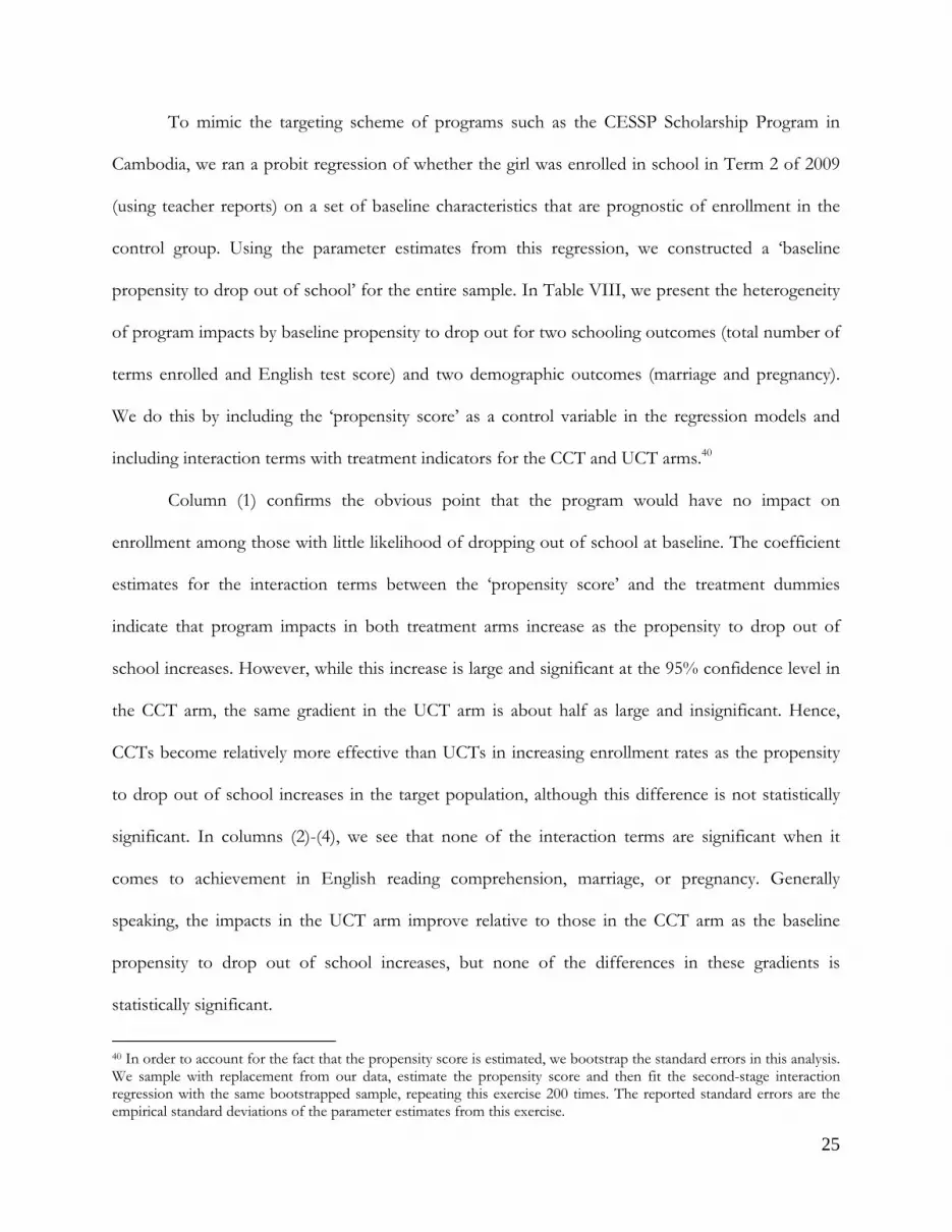
To mimic the targeting scheme of programs such as the CESSP Scholarship Program in

Cambodia, we ran a probit regression of whether the girl was enrolled in school in Term 2 of 2009

(using teacher reports) on a set of baseline characteristics that are prognostic of enrollment in the

control group. Using the parameter estimates from this regression, we constructed a ‘baseline

propensity to drop out of school’ for the entire sample. In Table VIII, we present the heterogeneity

of program impacts by baseline propensity to drop out for two schooling outcomes (total number of

terms enrolled and English test score) and two demographic outcomes (marriage and pregnancy).

We do this by including the ‘propensity score’ as a control variable in the regression models and

including interaction terms with treatment indicators for the CCT and UCT arms.40

Column (1) confirms the obvious point that the program would have no impact on

enrollment among those with little likelihood of dropping out of school at baseline. The coefficient

estimates for the interaction terms between the ‘propensity score’ and the treatment dummies

indicate that program impacts in both treatment arms increase as the propensity to drop out of

school increases. However, while this increase is large and significant at the 95% confidence level in

the CCT arm, the same gradient in the UCT arm is about half as large and insignificant. Hence,

CCTs become relatively more effective than UCTs in increasing enrollment rates as the propensity

to drop out of school increases in the target population, although this difference is not statistically

significant. In columns (2)-(4), we see that none of the interaction terms are significant when it

comes to achievement in English reading comprehension, marriage, or pregnancy. Generally

speaking, the impacts in the UCT arm improve relative to those in the CCT arm as the baseline

propensity to drop out of school increases, but none of the differences in these gradients is

statistically significant.

40 In order to account for the fact that the propensity score is estimated, we bootstrap the standard errors in this analysis. We sample with replacement from our data, estimate the propensity score and then fit the second-stage interaction regression with the same bootstrapped sample, repeating this exercise 200 times. The reported standard errors are the empirical standard deviations of the parameter estimates from this exercise.

26

In this experiment, if cash transfers were offered only to those with a high propensity to

drop out of school at baseline, the program impacts would have been larger – especially with respect

to enrollment. This finding is to be expected as targeting those at high risk of dropping out of

school would reduce the number of transfers that are infra-marginal. However, such a targeting

scheme would not alter our conclusions regarding the relative merits of the CCT and the UCT

schemes: schooling gains would still be significantly higher in the CCT arm while UCTs would be

more effective in delaying marriage and pregnancy among school-age girls.41

Table IX repeats the exercise in Table VIII by replacing the propensity score with an

indicator for being sixteen years or older.42 Program impacts on enrollment do not vary significantly

by age group, i.e. CCTs outperform UCTs in raising enrollment for early adolescents as well as older

teenagers. However, with respect to English test scores, marriage, and pregnancy, we see that

targeting the program to early adolescents would tilt the scale towards a CCT, while targeting it to

older teenagers would clearly favor a UCT. For each of these three outcomes, the difference in the

coefficients for the interaction terms between the CCT and UCT arms is large and statistically

significant. The advantage in English test scores the CCT arm enjoys among early adolescents

disappears completely among girls sixteen or older at baseline.43 Similarly, while the UCT arm still

outperforms the CCT arm in preventing marriages and pregnancies among early adolescents, this

advantage is substantially larger among older teenagers.

41 We have also examined heterogeneity of program impacts using a household asset index to imitate the means-tested targeting schemes like the ones in Brazil or Mexico. We find that enrollment impacts in the UCT arm may improve somewhat under such a targeting scheme, but otherwise program impacts would not be significantly altered compared to a universal cash transfer program for never-married adolescent girls. 42 The legal age of marriage stood at 16 in Malawi by late 2009 (Nyasa Times September 22, 2009) and many girls aged 16 or older are attending primary or secondary school. In our study sample, 22% of students eligible to attend primary school at baseline were aged 16 or older. This share increases to 56% for those eligible to attend secondary school at baseline. 43 Among this group of older teenagers, the UCT group performs equally well in the test of cognitive skills and even outperforms the CCT arm in mathematics.

27

These findings suggest that a CCT may be preferred to a UCT if the program is targeted to

early adolescents. Among this group, the achievement gains in the CCT arm relative to the UCT arm

are the largest and the disadvantage with respect to teenage pregnancy the lowest. As girls get older,

this trade-off disappears: the gains in test scores are similar in both treatment arms among girls aged

sixteen or older at baseline, while the advantage with respect to delayed marriage and pregnancy in

the UCT arm over the CCT arm is very large. UCTs may be preferable to CCTs among this group

of older adolescents.

We conclude this section by examining the heterogeneity in program impacts by two

important program features that were randomly varied in this experiment: the identity of the transfer

recipient within the household and transfer size. Bursztyn and Coffman (2010) argue that policies

designed to promote school attendance might be more effective if they target the child instead of

focusing on parents because sub-optimal school attendance may be due to a parent-child conflict,

where the parents cannot enforce their desire that their children attend school. Similarly, World

Bank (2009) argues that “…the key parameter in setting benefit levels is the size of the elasticity of

the relevant outcomes to the benefit level.” However, random variation in these design parameters is

rarely observed in cash transfer programs around the world. In this experiment, separate transfers

were made to girls and their parents (or guardians), the size of each of which were randomly

determined. Table X presents the heterogeneity in program impacts by these two variables.

Column (1) shows program impacts on enrollment: the minimum total transfer amount

offered to the household ($5/month total, with $1 to the girl and $4 to the parents) seems to be

responsible for the entire program impact on the ‘total number of terms enrolled’ in the CCT arm.

Additional transfers offered to either party make little difference. In the UCT arm, however, the

28

effect of the minimum transfer offer is small and insignificant44, but enrollment increases 0.081

terms with each additional dollar offered to the parents over and above $4/month. The analysis

implies that giving an additional $5/month in transfers to the parents would barely allow the UCT

arm to reach the level of enrollment attained by the minimum transfer amounts in the CCT arm. As

the marginal administrative cost of a CCT program is likely to be only a small share of each dollar

transferred to beneficiary households, a CCT program offering $5/month would clearly be more

cost-effective in increasing enrollment than a UCT program offering the same amount.

For English test scores, the results are similar for the CCT arm: there is no indication that

additional amounts to the girls or their parents would improve test scores over and above the

minimum monthly transfer. Here, unlike enrollment, the coefficient in the UCT arm is similar to the

CCT arm at the minimum transfer amounts, although insignificant. For marriage, there is no

treatment impact at the minimum transfer amounts in the UCT arm, but each additional dollar

offered to the parents of a girl reduces her likelihood of getting married by Round 3 by 1.6 pp. The

marginal effect of a dollar offered to parents in the UCT arm is 2.0 pp larger than that in the CCT

arm (p-value=0.11). The minimum amounts transferred in the UCT arm seem to be responsible for

almost the entire program effect on preventing pregnancies in this group.

In summary, increasing transfer amounts or varying the recipient within the household has

no effect on any of the outcomes examined in this paper in the CCT arm; contract variation simply

does not seem to matter. In contrast, we find that outcomes vary with increased transfer offers to

the parents in the UCT arm: enrollment rates increase and the incidence of marriage declines as

parents are offered more money, but performance in test scores seems to suffer. Still, however,

replacing a CCT program that offers the minimum transfer amounts of $1 to the girl and $4 to her

parents with a UCT program that offers the parents larger transfer amounts would not be cost-

44 The difference between the CCT and UCT impacts on enrollment at the minimum transfer amount ($5/month total to the household) is significant at the 90% confidence level.

29

effective in improving schooling outcomes, but it would reduce marriage rates among teenage girls.

Furthermore, we find no evidence that increasing the share of transfers made directly to the child

rather than her parents would be effective in improving any of the outcomes studied here.

4. Robustness Checks

4.1 Spillover Effects of Assignment to Cash Transfer Locations

In this experiment, treatment status with respect to conditionality was assigned at the EA

level. Due to the proximity of EAs to each other, in is possible that the intermingling of students in

the two treatment arms led to a change in behavior in the outcomes of interest, thus biasing our

estimates of the marginal impact of the conditionality. One way of addressing this issue is to exploit

the variation in treatment status across the locations at which the monthly cash transfers were made

(Cash Transfer or CT locations). The CT location is the primary interface between beneficiaries and

the program, so it provides a natural place to examine heterogeneity of program impacts. The

locations were determined entirely by logistical concerns, and in many cases beneficiaries from

multiple EAs were assigned to the same CT point. This variation can be informative because we

would expect spillovers on the UCT arm to be stronger as the share of CCT beneficiaries at the CT

point, for whom attendance is monitored and payments are withheld for unsatisfactory attendance,

increases.

To test for this spillover of monitoring intensity, we calculate the number of girls attending

each CT point (which is endogenous), the number of EAs that are serviced by each CT point (as a

control for the heterogeneity of treatment status at a CT point, also endogenous), and the number of

conditional girls at each CT point (which is exogenous and random conditional upon the other two).

The evidence from Table XI shows no evidence of any such spillovers: girls in the UCT arm do not

behave differently when there is more intense monitoring of attendance around them. It appears

30

unlikely that our estimates of differential program impacts are influenced by spillovers due to the

proximity of girls with discordant treatment statuses.

4.2 Are the results robust to the handling of school fees under the program?

As described in Section 2, secondary schools are not free in Malawi and the offers in the

CCT arm included a promise to pay secondary school fees directly to the schools upon confirmation

of enrollment by the program administrators.45 To make the average transfer offers in the UCT arm

equal to that in the CCT arm, the average school fee amount was added to the cash transfer offers

of girls in the UCT arm who were eligible to attend secondary school at the beginning of the

program (see footnote 22 for a more detailed description of this process). The relevant group

eligible to attend secondary school at the outset of the program is those girls whose ‘highest grade

attended at baseline’ are equal to Standard 8 or higher.

To test whether program impacts are influenced by the fact that school fee compensation

was handled differently between the two treatment arms, we restrict our analysis to the sub-sample

for whom school fees were not an issue: those whose highest grade attended at baseline was

Standard 7 or lower. This group constitutes more than 56% of our study population. Columns (1)-

(4) in Table XII show that all the impact findings are qualitatively the same as the average program

impacts presented earlier, although there is less power due to the fact that sample size has been

roughly halved. The CCT arm still holds an advantage in schooling outcomes, while the incidences

of marriage and pregnancy are lower in the UCT arm.

Before the start of the second year of the program, all offers to those in the CCT and UCT

arms were renewed. While those in the CCT arm who became eligible to attend secondary school

still received offers for their secondary school fees to be paid, each offer in the UCT arm was

identical to the previous one, meaning that girls who became eligible to attend secondary school

45 Or, the students who paid their school fees could get reimbursed upon producing a receipt.

31

were not offered additional payments in lieu of school fees.46 This means that there is a group of

girls in the UCT arm whose second year offers were smaller than their counterparts in the CCT arm.

To examine whether this had an effect on differential program impacts, we rerun our impact

regressions excluding this group from our sample, which constitutes approximately 25% of our

target population. Columns (5)-(8) indicate that program impacts in this sub-sample are very similar

to those for the entire sample.47 We conclude that any influence of the way in which school fee

compensation was handled in the two treatment arms on program impacts is likely to be very small.

5. Concluding discussion and policy implications

This paper presented experimental evidence on the relative effectiveness of conditional and

unconditional cash transfer programs. The analysis focused on two sets of outcomes that are of

central importance to the long-term prospects of school-age girls: schooling and human capital

formation on the one hand; marriage and fertility on the other. The results show that CCTs

increased enrollment rates and improved regular attendance for those in school, both of which likely

contributed to a modest but significant improvement in English test scores over the UCT arm.

Teenage pregnancy and marriage rates, on the other hand, were substantially lower in the UCT than

the CCT arm.

The results on school enrollment differ from previous studies that considered the relative

effectiveness of UCTs vs. CCTs, although the difference is a matter of degree rather than direction.

46 While this could have been done in principle for everyone whose highest grade attended at baseline was Standard 7 (regardless of their actual school progress, which is endogenous to treatment), the study team opted not to do this for fear of UCT girls ‘sensing’ that the additional payments were intended for school fees, and thereby contaminating the ‘unconditional’ treatment arm. As described in Section, during the first offers, UCT girls were told that they were randomly selected to receive bonuses as an explanation of their additional payments. The study team felt that this was not feasible in Year 2. 47 Another way to address this question is to compare the two UCT cohorts that were just eligible to attend secondary school in Year 1 and Year 2. By comparing these two cohorts, we can examine whether girls in the UCT arm entering secondary school who did receive the additional payment fared better than the following cohort that did not. This analysis shows no sign of a differential impact for the cohort receiving the payment.

32

Analyses of Bolsa Escola in Brazil and PROGRESA in Mexico found that UCTs would have little, if

any, impact on school enrollment – implying that almost all of the impacts of these programs were

due to the schooling condition (Bourguignon, Ferreira, and Leite 2003; Todd and Wolpin 2006). In

the Malawi experiment, on the other hand, we find a modest impact on enrollment in the UCT arm,

and this effect is 43% as large as the CCT arm. Our study thus confirms that conditions attached to

cash transfer programs are effective in increasing enrollment, but the size of this effect is likely to be

smaller than suggested by earlier studies, at least for poorer countries like Malawi.

Not only is school enrollment significantly improved in the CCT arm over the UCT arm, but

the evidence presented shows that CCTs are more cost-effective in raising enrollment than UCTs in

this context. To achieve the same enrollment gain obtained from a $5/month total transfer in the

CCT arm, a transfer of more than $10 to the parents in the UCT arm is needed. This difference is

much larger than the additional cost of administering a CCT program – possibly by an order of

magnitude.48 Furthermore, the average number of payments in the CCT arm was approximately 14.1

(out of a possible total of 20 over two years), compared with 17.9 in the UCT arm, implying that the

actual amount of transfers made per person was 19% lower in the CCT arm over the two-year

intervention. Savings of this magnitude due to non-compliance with the schooling condition would

more than make up for the additional administrative cost of monitoring in most programs.

While CCTs were more cost-effective than UCTs in increasing school enrollment and

attendance, they had no effect on reducing the likelihood of teenage pregnancies or marriages. The

offer of a CCT appears to have been ineffective in dissuading those with a high propensity to drop

out of school from getting married and starting childbearing, especially among girls sixteen or older

48 World Bank (2009) cites Grosh et al. (2008) to report that the median administrative cost is 8% of total program costs in ten CCT programs for which administrative cost data were compiled by that study. Given that monitoring compliance with the schooling condition is only part of the administrative costs, the additional cost would be a few cents on the dollar. However, monitoring and enforcement of conditionality in many of these programs may not have been as thorough as they were in our experiment, which could reduce the relative effectiveness of CCTs compared with UCTs.

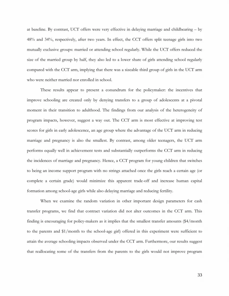
33

at baseline. By contrast, UCT offers were very effective in delaying marriage and childbearing – by

48% and 34%, respectively, after two years. In effect, the CCT offers split teenage girls into two

mutually exclusive groups: married or attending school regularly. While the UCT offers reduced the

size of the married group by half, they also led to a lower share of girls attending school regularly

compared with the CCT arm, implying that there was a sizeable third group of girls in the UCT arm

who were neither married nor enrolled in school.

These results appear to present a conundrum for the policymaker: the incentives that

improve schooling are created only by denying transfers to a group of adolescents at a pivotal

moment in their transition to adulthood. The findings from our analysis of the heterogeneity of

program impacts, however, suggest a way out. The CCT arm is most effective at improving test

scores for girls in early adolescence, an age group where the advantage of the UCT arm in reducing

marriage and pregnancy is also the smallest. By contrast, among older teenagers, the UCT arm

performs equally well in achievement tests and substantially outperforms the CCT arm in reducing

the incidences of marriage and pregnancy. Hence, a CCT program for young children that switches

to being an income support program with no strings attached once the girls reach a certain age (or

complete a certain grade) would minimize this apparent trade-off and increase human capital

formation among school-age girls while also delaying marriage and reducing fertility.

When we examine the random variation in other important design parameters for cash

transfer programs, we find that contract variation did not alter outcomes in the CCT arm. This

finding is encouraging for policy-makers as it implies that the smallest transfer amounts ($4/month

to the parents and $1/month to the school-age girl) offered in this experiment were sufficient to

attain the average schooling impacts observed under the CCT arm. Furthermore, our results suggest

that reallocating some of the transfers from the parents to the girls would not improve program

34

impacts under either treatment. Hence, while the idea of making part of the transfers directly to

adolescent girls may be attractive on its face, we find no evidence that it would be effective.49

As these findings are from a single experiment in one country, replication of the study in

other contexts is imperative. However, the experiment highlights some key points. First, the fact that

UCTs increase school enrollment indicates that poverty is an important cause of school dropout in

this population, and that poor parents will invest at least some of the additional funds from a

positive income shock towards the education of their daughters. Second, it is clear that CCTs

increase school enrollment over and above what is possible by a UCT. However, in the absence of a

market failure, such a large distortion in the consumption of education is inefficient.50 Policy-makers

planning to implement a CCT program should clearly articulate the market failures behind this

paternalistic motivation and, if possible, provide evidence of these externalities – private or social.

For example, we have not found any evidence of incomplete altruism – i.e. a conflict of interest

between the girls and their parents with respect to her education, which is sometimes mentioned as a

justification of a preference for CCTs over UCTs. Finally, the need to specify the reasons for

attaching conditions to cash transfer programs becomes even more significant in light of the

evidence that UCTs are substantially more effective than CCTs in delaying marriages and

childbearing among adolescent girls.

CCT programs create incentives for individuals to change their behaviors by denying

transfers to those who fail to satisfy the conditions. However, at least some of these individuals

come from vulnerable households and are also in need of income support. Our findings suggest that

UCTs to such households can improve important outcomes even though they are not as successful 49 The readers should note, however, that there was no cell in the experiment in which the transfer to the girl (or her parents) was equal to zero. It is possible that even a $1/month transfer made directly to the girls was more effective than adding that small amount to the transfers made to the parents. Our results are clear that marginal effect of reallocating any amount above the $1/month given to the girl would not improve outcomes. 50 In this context, credit market failures would not be a justification for CCTs as UCTs would be sufficient to relax credit constraints. Another market failure, such as lack of information, hyperbolic discounting, or positive spillover effects, is necessary to justify preferring CCTs over UCTs.

35

in improving schooling outcomes as CCTs. This paper makes clear that while CCT programs may be

more effective than UCTs in obtaining the desired behavior change, they can also undermine the

social protection dimension of cash transfer programs.

GEORGE WASHINGTON UNIVERSITY

UNIVERSITY OF CALIFORNIA, SAN DIEGO

THE WORLD BANK

APPENDIX A: OFFER LETTERS

CCT Offer Letter

The Zomba Cash Transfer Program (ZCTP)

with funding from the World Bank, would

like to offer you, ___[NAME]___, a cash

transfer to help you and your family with the

burdens of school attendance for the 2008

school year. By accepting this offer, in return

for going to school you will be given

___[AMOUNT]___ kwacha per month. If

you attend secondary school, your fees for the

2008 school year will be paid directly to your

school at the beginning of each term.

The payments to you and your family will be

made on a monthly basis beginning in

February, and will continue for 10 months

through November 2008.

You are receiving this money in order to help

you return to school or stay in school. In

order to receive this money you MUST

attend school at least 80% of the days for

which your school is in session.

UCT Offer Letter

The Zomba Cash Transfer Program (ZCTP),

with funding from the World Bank, would

like to offer you, ___[NAME]___, a cash

transfer to help you and your family. By

accepting this offer you will be given

___[AMOUNT]___ kwacha per month.

The payments to you and your family will be

made on a monthly basis beginning in

February, and will continue for 10 months

through November 2008.

These monthly transfer amounts specified

above are given to you as a result of a lottery.

You are not required to do anything more to

receive this money. You will receive this

money for 10 months between February and

November, 2008.

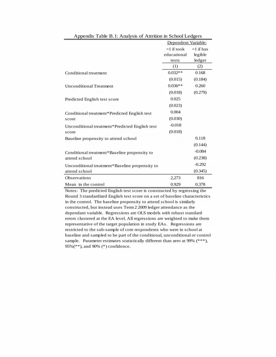
=1 if took educational

tests

=1 if has legible ledger

(1) (2)

Conditional treatment 0.032** 0.168

(0.015) (0.184)

Unconditional Treatment 0.036** 0.260

(0.018) (0.279)

Predicted English test score 0.025

(0.023)

0.004

(0.030)

-0.018

(0.018)

Baseline propensity to attend school 0.118

(0.144)

-0.084

(0.238)

-0.292

(0.345)

Observations 2,273 816

Mean in the control 0.929 0.378

Appendix Table B.1: Analysis of Attrition in School Ledgers

Notes: The predicted English test score is constructed by regressing the Round 3 standardized English test score on a set of baseline characteristics in the control. The baseline propensity to attend school is similarly constructed, but instead uses Term 2 2009 ledger attendance as the dependant variable. Regressions are OLS models with robust standard errors clustered at the EA level. All regressions are weighted to make them representative of the target population in study EAs. Regressions are restricted to the sub-sample of core respondents who were in school at baseline and sampled to be part of the conditional, unconditional or control sample. Parameter estimates statistically different than zero at 99% (***), 95%(**), and 90% (*) confidence.

Dependent Variable:

Unconditional treatment*Baseline propensity to attend school

Conditional treatment*Baseline propensity to attend school

Conditional treatment*Predicted English test score

Unconditional treatment*Predicted English test score

38

References

Adato, Michelle, and Lucy Bassett, “Social Protection to Support Vulnerable Children and Families:

the potential of cash transfers to protect education, health and nutrition,” AIDS Care, 21(2009),

60-75.

Akinbami, Lara J., Kenneth C. Schoendorf, and John L. Kiely, “Risk of Preterm Birth in

Multiparous Teenagers,” Archives of Pediatrics and Adolescent Medicine, 154(2000): 1101-1107.

Ashcraft, Adam, and Kevin Lang, “The Consequences of Teenage Childbearing,” NBER Working

Paper 12485. National Bureau of Economic Research, Cambridge, MA, 2006.

Baird, Sarah, and Berk Özler, “Examining the Reliability of Self-Reported Data on School

Participation,” unpublished manuscript, 2010.

Barrera-Osorio, Felipe, Marianne Bertrand, Leigh L. Linden, and Francisco Perez-Calle, “Improving

the Design of Conditional Transfer Programs: Evidence from a Randomized Education

Experiment in Colombia,” American Economic Journal: Applied Economics, forthcoming, 2010.

Barrett, Christopher, and Michael Carter, “The Power and Pitfalls of Experiments in Development

Economics: Some Non-Random Reflections,” Applied Economic Perspectives and Policies,

forthcoming, 2011.

Behrman, Jere R., Susan W. Parker, and Petra E. Todd, "Medium-Term Impacts of the

Oportunidades Conditional Cash Transfer Program on Rural Youth in Mexico" in Poverty,

Inequality and Policy in Latin America, eds. Stephan Klasen and Felicitas Nowak-Lehman, 219-70

Cambridge, MA, MIT Press, 2009.

Behrman, Jere R., Piyali Sengupta, and Petra Todd, “Progressing through PROGRESA: An Impact

Assessment of a School Subsidy Experiment in Rural Mexico,” Economic Development and Cultural

Change, 54 (2005), Issue 1, 237-275.

39

Blau, Francine, and Lawrence Kahn, “Do Cognitive Test Scores Explain Higher U.S. Wage

Inequality?” Review of Economics and Statistics, 87(2005), pp. 184-193.

Bloom, David E., David Canning, Günther Fink, and Jocelyn E. Finlay, “Fertility, Female Labor

Force Participation, and the Demographic Dividend,” Journal of Economic Growth, 14(2009), 79-

101.

Bourguignon, François, Francisco H.G. Ferreira, and Phillippe G. Leite, “Conditional Cash

Transfers, Schooling, and Child Labor: Micro-Simulating Brazil’s Bolsa Escola Program,” The

World Bank Economic Review, 17(2003), 229-254.

Bruhn, Miriam, and David McKenzie, "In Pursuit of Balance: Randomization in Practice in

Development Field Experiments," American Economic Journal: Applied Economics, 1(2008), 200-232.

Bursztyn, Leonardo, and Lucas Coffman, “The Schooling Decision: Family Preferences,

Intergenerational Conflict, and Moral Hazard in the Brazilian Favelas,” unpublished manuscript.

http://www.anderson.ucla.edu/faculty/leonardo.bursztyn/Schooling_Decision_10_18_10.pdf,

2010.

Case, Anne, Victoria Hosegood, and Frances Lund, “The reach and impact of Child Support Grants:

Evidence from KwaZulu-Natal,” Development Southern Africa, 22(2005), 467-482.

Cunha, Jesse M., “Testing Paternalism: Cash vs. In-kind Transfers in Rural Mexico,” unpublished

manuscript. http://www.stanford.edu/~jcunha/Cunha_Testing_Paternalism.pdf, 2010.

Dahl, Gordon B., “Early Teen Marriage and Future Poverty,” Demography, 47(2010): 689-718.

de Brauw, Alan, and John Hoddinott, "Must Conditional Cash Transfer Programs be Conditioned

to be Effective? The Impact of Conditioning Transfers on School Enrollment in Mexico,"

Journal of Development Economics, forthcoming, 2010.

40

de Janvry, Alain, Frederico Finan, Elisabeth Sadoulet, and Renos Vakis, “Can conditional cash

transfer programs serve as safety nets in keeping children at school and from working when

exposed to shocks?” Journal of Development Economics, 79(2006), 349-373.

de Janvry, Alain, and Elisabeth Sadoulet, “Making Conditional Cash Transfer Programs More

Efficient: Designing for Maximum Effect of the Conditionality,” The World Bank Economic Review,

20(2006), 1-29.

Duflo, Esther, “Grandmothers and Granddaughters: Old-Age Pensions and Intrahousehold

Allocation in South Africa,” The World Bank Economic Review, 17(2003), 1-25.

Dzinjalamala, Fraction, “Malaria,” in The Epidemiology of Malawi, eds. (Geubbels and Bowie), College

of Medicine, University of Malawi, 2009.

http://www.medcol.mw/commhealth/publications/epi%20book/epidemiology%20book.htm

Edmonds, Eric V., “Child Labor and Schooling Responses to Anticipated Income in South Africa,”

Journal of Development Economics, 81(2006), 386-414.

Edmonds, Eric V., and Norbert Schady, “Poverty Alleviation and Child Labor,” NBER Working

Paper 15345. National Bureau of Economic Research, Cambridge, MA, 2009.

Field, Erica, and Attila Ambrus, “Early Marriage, Age of Menarche, and Female Schooling

Attainment in Bangladesh,” Journal of Political Economy, 116(2008): 881-930.

Filmer, Deon, and Norbert Schady, “Does More Cash in Conditional Cash Transfer Programs

Always Lead to Larger Impacts on School Attendance?” Journal of Development Economics,

forthcoming, 2010.

___________, “School Enrollment, Selection and Test Scores,” Policy Research Working Paper

Series 4998, The World Bank, 2009.

Fletcher, Jason M., and Barbara L. Wolfe, “Education and Labor Market Consequences of Teenage

Childbearing: Evidence Using the Timing of Pregnancy Outcomes and Community Fixed

41

Effects,” NBER Working Paper 13847. National Bureau of Economic Research, Cambridge,

MA, 2008.

Goldin, Claudia, and Lawrence F. Katz, “The Power of the Pill: Oral Contraceptives and Women’s

Career and Marriage Decisions,” Journal of Political Economy, 110(2002): 730-770.

Hanlon, Joseph, Armando Barrientos, and David Hulme, Just Give Money to the Poor: The Development

Revolution from the South, Kumarian Press: USA, 2010.

Hanushek, Eric V., and Ludger Woessmann, “Do Better Schools Lead to More Growth? Cognitive

Skills, Economic Outcomes, and Causation,” NBER Working Paper 14633. National Bureau of

Economic Research, Cambridge, MA, 2009

Horgan, Richard P., and Louise C. Kenny, “Management of Teenage Pregnancy,” The Obstetrician &

Gynaecologist, 9(2007): 153–158.

Hotz, V. Joseph, Susan W. McElroy, and Seth G. Sanders, “Teenage Childbearing and Its Life Cycle

Consequences: Exploiting a Very Natural Experiment” Journal of Human Resources 40(2005): 683–

715.

Jensen, Robert, and Rebecca Thornton, “Early female marriage in the developing world,” Gender and

Development, 11(2003): 9-19.

Kremer, Michael, Edward Miguel, and Rebecca Thornton, “Incentives to Learn,” The Review of

Economics and Statistics, 91(2009), 437-456.

Macours, Karen, Norbert Schady, and Renos Vakis, “Cash Transfers, Behavioral Changes, and

Cognitive Development in Early Childhood: Evidence from a Randomized Experiment,” Policy

Research Working Paper Series 4759, The World Bank, 2008.

Miguel, Edward, and Michael Kremer, “Worms: Identifying Impacts on Education and Health in the

Presence of Treatment Externalities,” Econometrica, 72(2004), 159-217.

42

Miller, Candace, and Maxton Tsoka, “Evaluating the Mchinji Social Cash Transfer Pilot,”

http://www.unicef.org/socialpolicy/files/REvised_Presentation_Evaluating_the_Mchinji_Socia

l_Cash_Transfer_Pilot_2_July_07.pdf.

Nyasa Times, “Debate over Recommended Marriage Age for Girls Continues in Malawi,” September

22, 2009. (http://www.nyasatimes.com/features/debate-over-recommended-marriage-age-for-

girls-continues-in-malawi.html)

Paxson, Christina, and Norbert Schady, “Does money matter? The Effects of Cash Transfers on

Child Health and Development in Rural Ecuador,” Policy Research Working Paper Series 4226,

The World Bank, 2007.

Schady, Norbert R., and Maria Caridad Araujo, “Cash Transfers, Conditions, and School Enrollment

in Ecuador,” Economía, 8(2008), 43-70.

Schultz, T. Paul, “School Subsidies for the Poor: Evaluating the Mexican Progresa Poverty

Program,” Journal of Development Economics, 74(2004), 199-250.

Smith, Gordon C. S., and Jill P. Pell, “Teenage Pregnancy and Risk of Adverse Perinatal Outcomes

Associated with First and Second Births: Population Based Retrospective Cohort Study,” BMJ,

323(2001): 1-5.

Todd, Petra E., and Kenneth I. Wolpin, "Assessing the Impact of a School Subsidy Program in

Mexico: Using a Social Experiment to Validate a Dynamic Behavioral Model of Child Schooling

and Fertility," American Economic Review, 96(2006), 1384–1417.

World Bank, Conditional Cash Transfers: Reducing Present and Future Poverty, eds: Fiszbein and Schady.

World Bank Publications, Washington, DC, USA, 2009.

World Development Indicators Database. 2010. Accessed November, 2010.

=1 if surveyed in round 3

=1 if surveyed in

all three rounds

=1 if took educational

test

=1 if information

found in round 2 school survey

=1 if information

found in round 3 school survey

=1 if legible ledger found

(1) (2) (3) (4) (5) (6)

Conditional treatment 0.020 0.021 0.029* 0.033 -0.000 0.116*

(0.015) (0.030) (0.016) (0.024) (0.027) (0.064)

Unconditional treatment 0.021 0.030 0.035* -0.029 0.014 0.061

(0.019) (0.024) (0.020) (0.053) (0.028) (0.077)

Mean in control 0.946 0.893 0.929 0.890 0.935 0.378

Sample Size 2,284 2,284 2,284 2,284 983 821

Prob > F(Conditional=Unconditional) 0.965 0.797 0.801 0.246 0.627 0.513

Dependent Variable:

Notes: Regressions are OLS models with robust standard errors clustered at the EA level. All regressions are weighted to make them representative of the target population in study EAs. Regressions are restricted to the sub-sample of core respondents who were in school at baseline and sampled to be part of the conditional, unconditional or control sample. Parameter estimates statistically different than zero at 99% (***), 95% (**), and 90% (*) confidence.

Table I: Analysis of Attrition

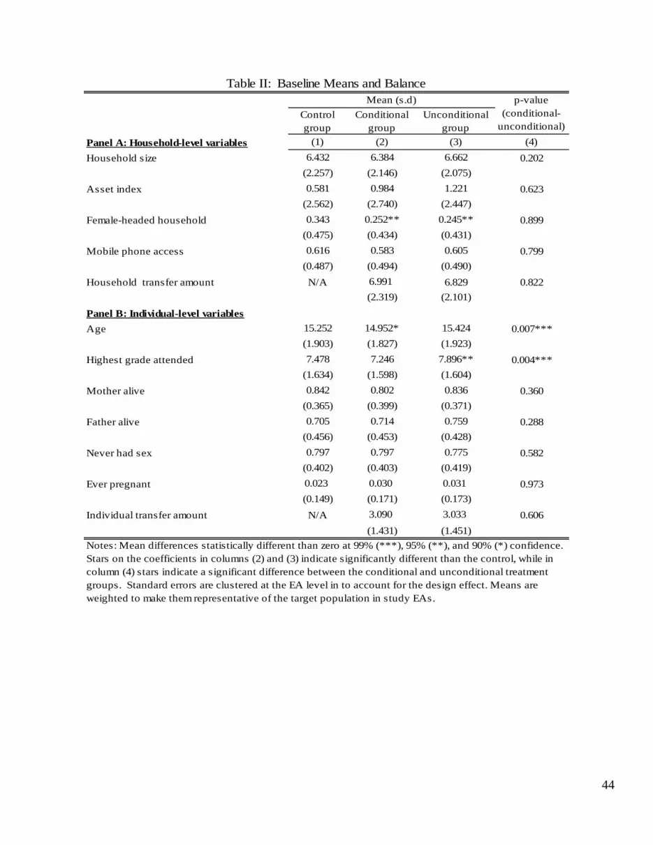
44

Control group

Conditional group

Unconditional group

Panel A: Household-level variables (1) (2) (3) (4)

Household size 6.432 6.384 6.662 0.202

(2.257) (2.146) (2.075)

Asset index 0.581 0.984 1.221 0.623

(2.562) (2.740) (2.447)

Female-headed household 0.343 0.252** 0.245** 0.899

(0.475) (0.434) (0.431)

Mobile phone access 0.616 0.583 0.605 0.799

(0.487) (0.494) (0.490)

Household transfer amount N/A 6.991 6.829 0.822

(2.319) (2.101)

Panel B: Individual-level variables

Age 15.252 14.952* 15.424 0.007***

(1.903) (1.827) (1.923)

Highest grade attended 7.478 7.246 7.896** 0.004***

(1.634) (1.598) (1.604)

Mother alive 0.842 0.802 0.836 0.360

(0.365) (0.399) (0.371)

Father alive 0.705 0.714 0.759 0.288

(0.456) (0.453) (0.428)

Never had sex 0.797 0.797 0.775 0.582

(0.402) (0.403) (0.419)

Ever pregnant 0.023 0.030 0.031 0.973

(0.149) (0.171) (0.173)

Individual transfer amount N/A 3.090 3.033 0.606

(1.431) (1.451)

Mean (s.d) p-value (conditional-

unconditional)

Notes: Mean differences statistically different than zero at 99% (***), 95% (**), and 90% (*) confidence. Stars on the coefficients in columns (2) and (3) indicate significantly different than the control, while in column (4) stars indicate a significant difference between the conditional and unconditional treatment groups. Standard errors are clustered at the EA level in to account for the design effect. Means are weighted to make them representative of the target population in study EAs.

Table II: Baseline Means and Balance

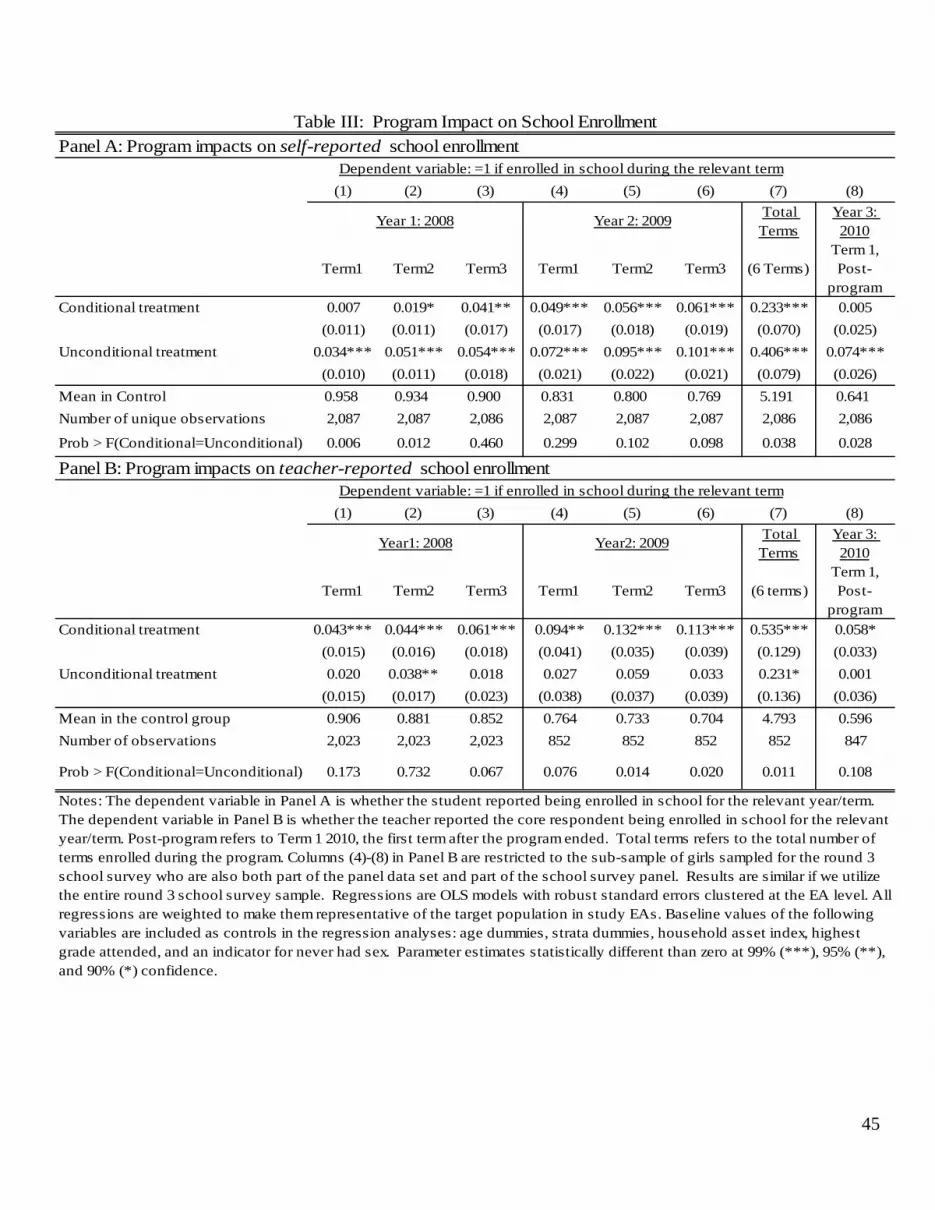
45

(1) (2) (3) (4) (5) (6) (7) (8)

Total Terms

Year 3: 2010

Term1 Term2 Term3 Term1 Term2 Term3 (6 Terms)Term 1, Post-

program

Conditional treatment 0.007 0.019* 0.041** 0.049*** 0.056*** 0.061*** 0.233*** 0.005

(0.011) (0.011) (0.017) (0.017) (0.018) (0.019) (0.070) (0.025)

Unconditional treatment 0.034*** 0.051*** 0.054*** 0.072*** 0.095*** 0.101*** 0.406*** 0.074***

(0.010) (0.011) (0.018) (0.021) (0.022) (0.021) (0.079) (0.026)

Mean in Control 0.958 0.934 0.900 0.831 0.800 0.769 5.191 0.641

Number of unique observations 2,087 2,087 2,086 2,087 2,087 2,087 2,086 2,086

Prob > F(Conditional=Unconditional) 0.006 0.012 0.460 0.299 0.102 0.098 0.038 0.028

(1) (2) (3) (4) (5) (6) (7) (8)

Total Terms

Year 3: 2010

Term1 Term2 Term3 Term1 Term2 Term3 (6 terms)Term 1, Post-

program

Conditional treatment 0.043*** 0.044*** 0.061*** 0.094** 0.132*** 0.113*** 0.535*** 0.058*

(0.015) (0.016) (0.018) (0.041) (0.035) (0.039) (0.129) (0.033)

Unconditional treatment 0.020 0.038** 0.018 0.027 0.059 0.033 0.231* 0.001

(0.015) (0.017) (0.023) (0.038) (0.037) (0.039) (0.136) (0.036)

Mean in the control group 0.906 0.881 0.852 0.764 0.733 0.704 4.793 0.596

Number of observations 2,023 2,023 2,023 852 852 852 852 847

Prob > F(Conditional=Unconditional) 0.173 0.732 0.067 0.076 0.014 0.020 0.011 0.108

Table III: Program Impact on School Enrollment

Dependent variable: =1 if enrolled in school during the relevant term

Year1: 2008 Year2: 2009

Notes: The dependent variable in Panel A is whether the student reported being enrolled in school for the relevant year/term. The dependent variable in Panel B is whether the teacher reported the core respondent being enrolled in school for the relevant year/term. Post-program refers to Term 1 2010, the first term after the program ended. Total terms refers to the total number of terms enrolled during the program. Columns (4)-(8) in Panel B are restricted to the sub-sample of girls sampled for the round 3 school survey who are also both part of the panel data set and part of the school survey panel. Results are similar if we utilize the entire round 3 school survey sample. Regressions are OLS models with robust standard errors clustered at the EA level. All regressions are weighted to make them representative of the target population in study EAs. Baseline values of the following variables are included as controls in the regression analyses: age dummies, strata dummies, household asset index, highest grade attended, and an indicator for never had sex. Parameter estimates statistically different than zero at 99% (***), 95% (**), and 90% (*) confidence.

Panel A: Program impacts on self-reported school enrollment

Year 1: 2008 Year 2: 2009

Dependent variable: =1 if enrolled in school during the relevant term

Panel B: Program impacts on teacher-reported school enrollment

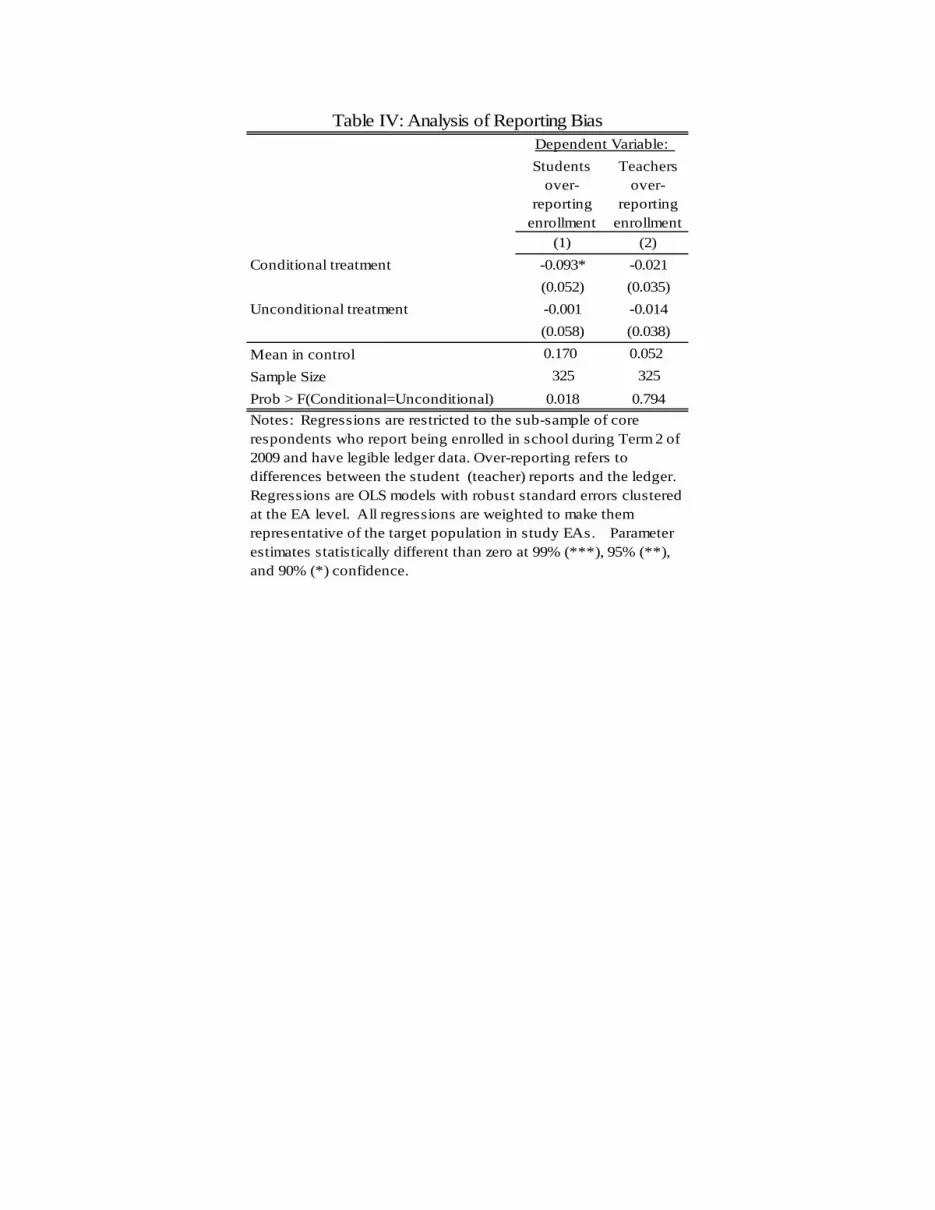
Students over-

reporting enrollment

Teachers over-

reporting enrollment

(1) (2)

Conditional treatment -0.093* -0.021

(0.052) (0.035)

Unconditional treatment -0.001 -0.014

(0.058) (0.038)

Mean in control 0.170 0.052

Sample Size 325 325

Prob > F(Conditional=Unconditional) 0.018 0.794

Dependent Variable:

Table IV: Analysis of Reporting Bias

Notes: Regressions are restricted to the sub-sample of core respondents who report being enrolled in school during Term 2 of 2009 and have legible ledger data. Over-reporting refers to differences between the student (teacher) reports and the ledger. Regressions are OLS models with robust standard errors clustered at the EA level. All regressions are weighted to make them representative of the target population in study EAs. Parameter estimates statistically different than zero at 99% (***), 95% (**), and 90% (*) confidence.

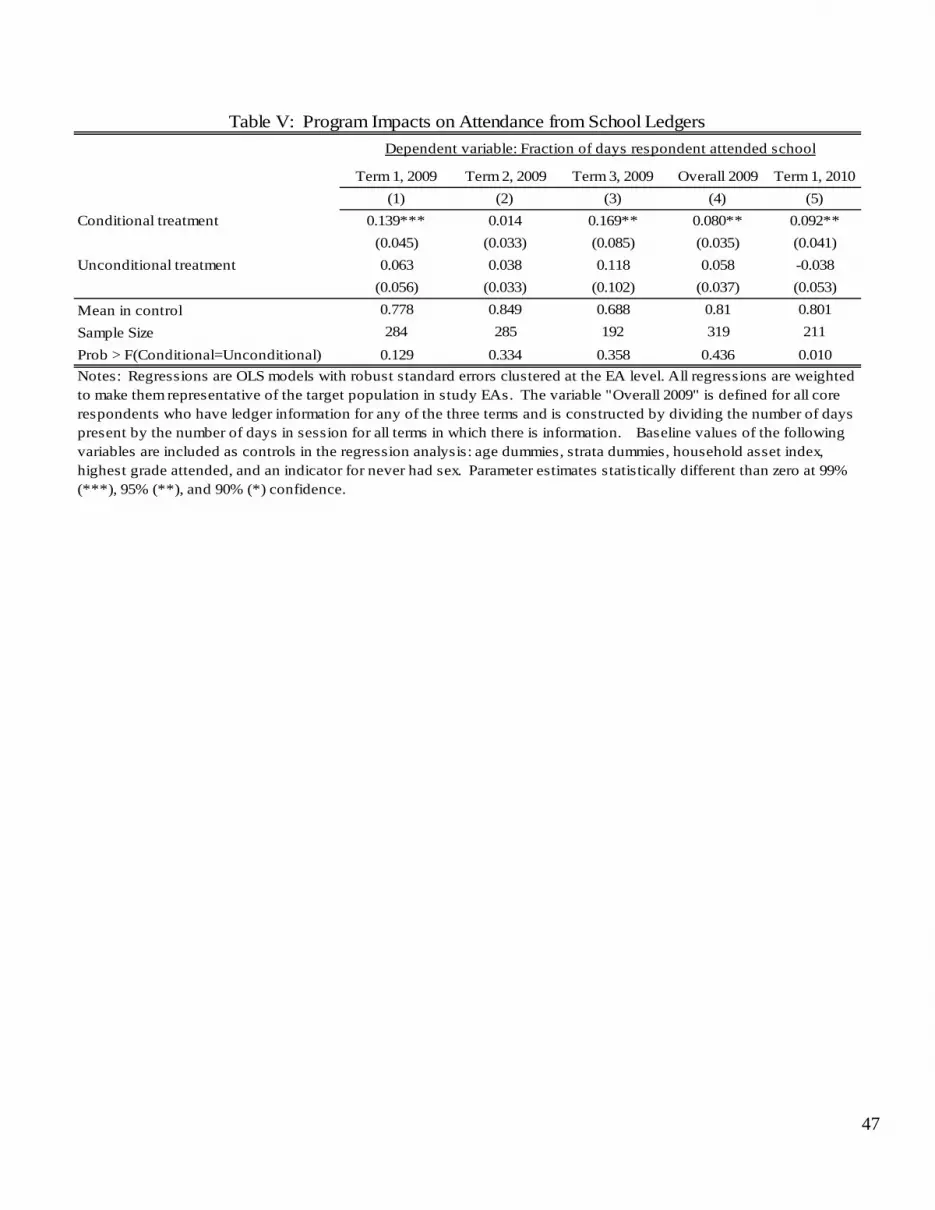
47

Term 1, 2009 Term 2, 2009 Term 3, 2009 Overall 2009 Term 1, 2010

(1) (2) (3) (4) (5)

Conditional treatment 0.139*** 0.014 0.169** 0.080** 0.092**

(0.045) (0.033) (0.085) (0.035) (0.041)

Unconditional treatment 0.063 0.038 0.118 0.058 -0.038

(0.056) (0.033) (0.102) (0.037) (0.053)

Mean in control 0.778 0.849 0.688 0.81 0.801

Sample Size 284 285 192 319 211

Prob > F(Conditional=Unconditional) 0.129 0.334 0.358 0.436 0.010

Dependent variable: Fraction of days respondent attended school

Notes: Regressions are OLS models with robust standard errors clustered at the EA level. All regressions are weighted to make them representative of the target population in study EAs. The variable "Overall 2009" is defined for all core respondents who have ledger information for any of the three terms and is constructed by dividing the number of days present by the number of days in session for all terms in which there is information. Baseline values of the following variables are included as controls in the regression analysis: age dummies, strata dummies, household asset index, highest grade attended, and an indicator for never had sex. Parameter estimates statistically different than zero at 99% (***), 95% (**), and 90% (*) confidence.

Table V: Program Impacts on Attendance from School Ledgers

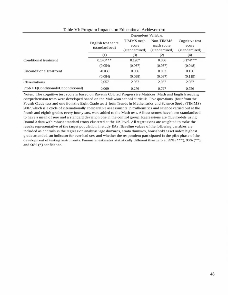
48

English test score (standardized)

TIMMS math score

(standardized)

Non-TIMMS math score

(standardized)

Cognitive test score

(standardized)

(1) (3) (2) (4)

Conditional treatment 0.140*** 0.120* 0.086 0.174***

(0.054) (0.067) (0.057) (0.048)

Unconditional treatment -0.030 0.006 0.063 0.136

(0.084) (0.098) (0.087) (0.119)

Observations 2,057 2,057 2,057 2,057

Prob > F(Conditional=Unconditional) 0.069 0.276 0.797 0.756

Table VI: Program Impacts on Educational AchievementDependent Variable:

Notes: The cognitive test score is based on Raven's Colored Progressive Matrices. Math and English reading comprehension tests were developed based on the Malawian school curricula. Five questions (four from the Fourth Grade test and one from the Eight Grade test) from Trends in Mathematics and Science Study (TIMMS) 2007, which is a cycle of internationally comparative assessments in mathematics and science carried out at the fourth and eighth grades every four years, were added to the Math test. All test scores have been standardized to have a mean of zero and a standard deviation one in the control group. Regressions are OLS models using Round 3 data with robust standard errors clustered at the EA level. All regressions are weighted to make the results representative of the target population in study EAs. Baseline values of the following variables are included as controls in the regression analysis: age dummies, strata dummies, household asset index, highest grade attended, an indicator for ever had sex, and whether the respondent participated in the pilot phase of the development of testing instruments. Parameter estimates statistically different than zero at 99% (***), 95% (**), and 90% (*) confidence.

49

=1 if ever married =1 if ever pregnant

(1) (2)

Conditional treatment, 2009 -0.027 0.002

(0.031) (0.035)

Unconditional treatment, 2009 -0.086*** -0.077***

(0.027) (0.029)

Conditional treatment, 2008 0.003 -0.001

(0.013) (0.015)

Unconditional treatment, 2008 -0.027** -0.007

(0.012) (0.014)

Time trend, 2009 0.180*** 0.224***

(0.016) (0.016)

Time trend, 2008 0.043*** 0.066***

(0.007) (0.008)

Number of unique observations 2,089 2,089

Baseline control mean 0.000 0.023

Prob > F(Conditional=Unconditional), 2008 0.030 0.704

Prob > F(Conditional=Unconditional), 2009 0.093 0.044

Table VII: Program Impacts on Marriage and Pregnancy

Notes: The dependent variables are having been ever married or ever pregnant at the time of the relevant survey. Regressions are individual fixed-effects models with robust standard errors clustered at the EA level. All regressions are weighted to make the results representative of the target population in study EAs. Parameter estimates statistically different than zero at 99% (***), 95% (**), and 90% (*) confidence.

Dependent variable:

50

Total number of terms enrolled

(school survey)

Standardized English test

score

=1 if ever married

=1 if ever pregnant

(1) (2) (3) (4)

Conditional treatment 0.057 0.104 -0.032 -0.027

(0.168) (0.106) (0.021) (0.029)

Unconditional treatment 0.002 -0.165 -0.009 -0.044*

(0.194) (0.143) (0.022) (0.025)

Dropout propensity -3.733*** -0.706***

(0.760) (0.195)

Conditional treatment*dropout propensity 1.724** 0.117 0.061 0.139

(0.714) (0.263) (0.136) (0.148)

Unconditional treatment*dropout propensity 0.888 0.441 -0.229 -0.084

(0.835) (0.301) (0.151) (0.189)

Time trend 0.004 0.039**

(0.013) (0.017)

Time trend*dropout propensity 0.557*** 0.590***

(0.094) (0.116)

Number of unique observations 843 2,057 2,089 2,089

Prob > F(Conditional=Unconditional) 0.731 0.118 0.343 0.564

Prob > F(Conditional*Dropout=Unconditional*Dropout) 0.369 0.452 0.156 0.287

Table VIII: Heterogeneity of Program Impacts by Dropout Propensity

Dependent Variable:

Notes: The dropout propensity is constructed by regressing an indicator for whether the girl was in school during Term 2, 2009 according to the school survey on a set of baseline variables in the control group. For the number of total terms enrolled and standardized English test score, regressions are OLS models using Round 3 data with robust standard errors clustered at the EA level. Baseline values of the following variables are included as controls in the regression analysis: age dummies, strata dummies, household asset index, highest grade attended, and an indicator for ever had sex. Marriage and pregnancy regressions are individual fixed-effects models with robust standard errors clustered at the EA level using data from baseline and Round 3. Standard errors for dropout propensity and the interactions terms are bootstrapped in order to account for the fact that the propensity score is estimated. All regressions are weighted to make the results representative of the target population in study EAs. Parameter estimates statistically different than zero at 99% (***), 95% (**), and 90%(*) confidence.

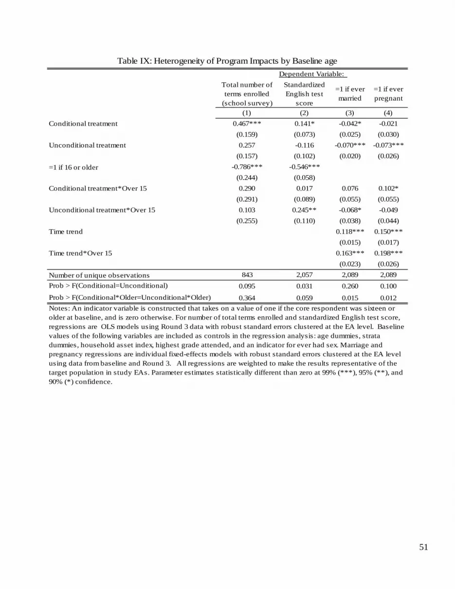
51

Total number of terms enrolled

(school survey)

Standardized English test

score

=1 if ever married

=1 if ever pregnant

(1) (2) (3) (4)

Conditional treatment 0.467*** 0.141* -0.042* -0.021

(0.159) (0.073) (0.025) (0.030)

Unconditional treatment 0.257 -0.116 -0.070*** -0.073***

(0.157) (0.102) (0.020) (0.026)

=1 if 16 or older -0.786*** -0.546***

(0.244) (0.058)

Conditional treatment*Over 15 0.290 0.017 0.076 0.102*

(0.291) (0.089) (0.055) (0.055)

Unconditional treatment*Over 15 0.103 0.245** -0.068* -0.049

(0.255) (0.110) (0.038) (0.044)

Time trend 0.118*** 0.150***

(0.015) (0.017)

Time trend*Over 15 0.163*** 0.198***

(0.023) (0.026)

Number of unique observations 843 2,057 2,089 2,089

Prob > F(Conditional=Unconditional) 0.095 0.031 0.260 0.100

Prob > F(Conditional*Older=Unconditional*Older) 0.364 0.059 0.015 0.012

Table IX: Heterogeneity of Program Impacts by Baseline age

Notes: An indicator variable is constructed that takes on a value of one if the core respondent was sixteen or older at baseline, and is zero otherwise. For number of total terms enrolled and standardized English test score, regressions are OLS models using Round 3 data with robust standard errors clustered at the EA level. Baseline values of the following variables are included as controls in the regression analysis: age dummies, strata dummies, household asset index, highest grade attended, and an indicator for ever had sex. Marriage and pregnancy regressions are individual fixed-effects models with robust standard errors clustered at the EA level using data from baseline and Round 3. All regressions are weighted to make the results representative of the target population in study EAs. Parameter estimates statistically different than zero at 99% (***), 95% (**), and 90% (*) confidence.

Dependent Variable:

52

Total number of terms enrolled

(school survey)

Standardized English test score

=1 if ever married=1 if ever pregnant

(1) (2) (3) (4)

Conditional treatment, individual amount 0.024 -0.032 -0.014 -0.002

(0.051) (0.029) (0.009) (0.016)

Unconditional treatment, individual amount -0.048 -0.019 -0.010 0.006

(0.064) (0.038) (0.011) (0.014)

Conditional treatment, household amount -0.027 -0.000 0.005 0.000

(0.035) (0.016) (0.010) (0.014)

Unconditional treatment, household amount 0.081*** -0.058** -0.016** -0.008

(0.031) (0.029) (0.007) (0.008)

Conditional treatment, minimum transfer amounts 0.572*** 0.202* -0.012 0.005

(0.213) (0.118) (0.053) (0.072)

Unconditional treatment, minimum transfer amounts 0.094 0.175 -0.022 -0.067*

(0.167) (0.132) (0.032) (0.037)

Number of unique observations 852 2,057 2,089 2,089

Prob > F(Conditional=Unconditional), individual amount

0.390 0.788 0.765 0.707

Prob > F(Conditional=Unconditional), household amount

0.025 0.082 0.108 0.616

Prob > F(Conditional=Unconditional), minimum amount

0.046 0.877 0.863 0.350

Table X: Impacts of Household and Individual Transfer Amounts

Dependent variable:

Notes: For total number of terms enrolled and standardized English test score regressions are OLS models using Round 3 data with robust standard errors clustered at the EA level. Baseline values of the following variables are included as controls in the regression analysis: age dummies, strata dummies, household asset index, highest grade attended, and an indicator for ever had sex. Marriage and pregnancy regressions are individual fixed-effects models with robust standard errors clustered at the EA level using data from baseline and Round 3. All regressions are weighted to make the results representative of the target population in study EAs. Parameter estimates statistically different than zero at 99% (***), 95% (**), and 90% (*) confidence.

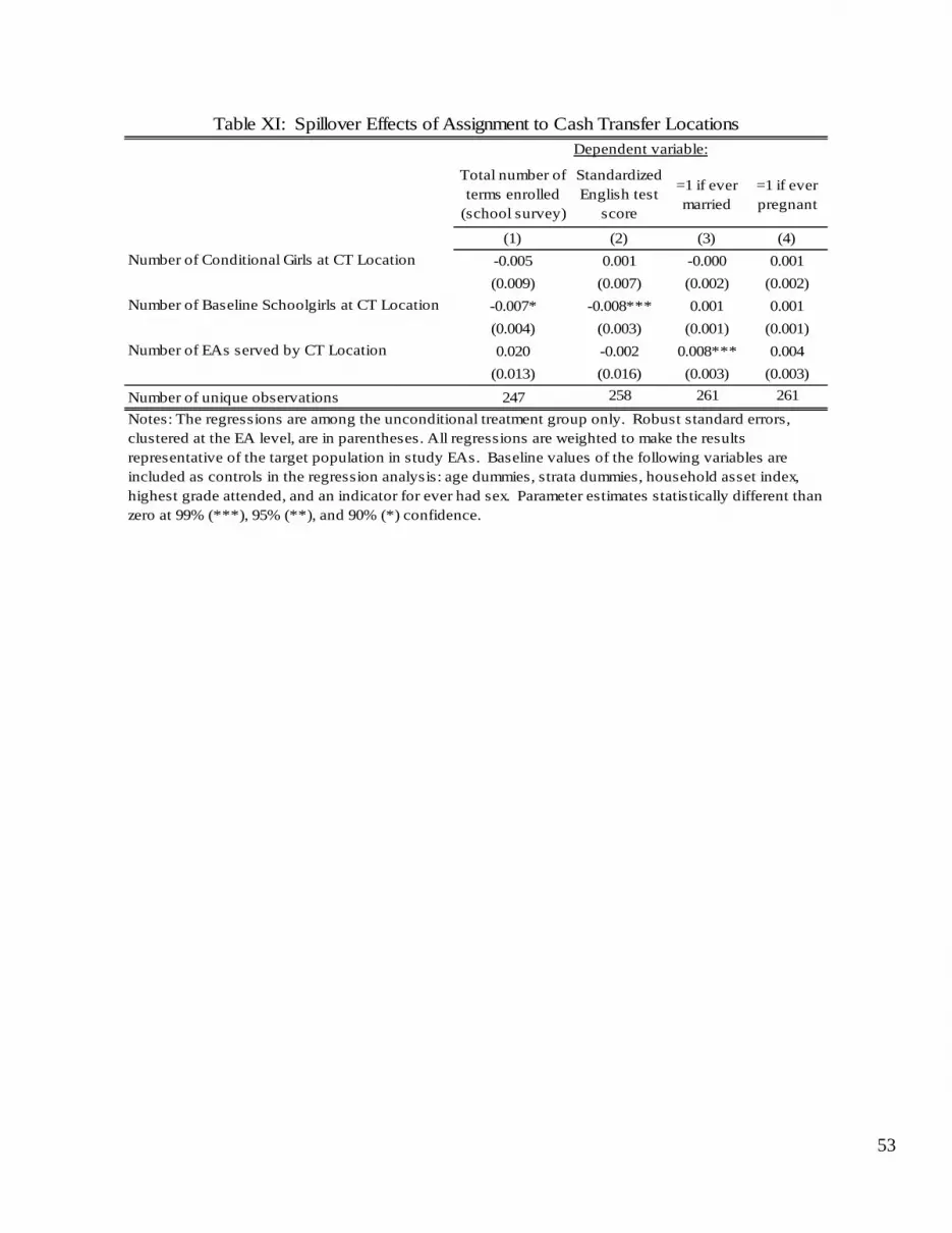
53

Total number of terms enrolled

(school survey)

Standardized English test

score

=1 if ever married

=1 if ever pregnant

(1) (2) (3) (4)

Number of Conditional Girls at CT Location -0.005 0.001 -0.000 0.001

(0.009) (0.007) (0.002) (0.002)

Number of Baseline Schoolgirls at CT Location -0.007* -0.008*** 0.001 0.001

(0.004) (0.003) (0.001) (0.001)

Number of EAs served by CT Location 0.020 -0.002 0.008*** 0.004

(0.013) (0.016) (0.003) (0.003)

Number of unique observations 247 258 261 261

Notes: The regressions are among the unconditional treatment group only. Robust standard errors, clustered at the EA level, are in parentheses. All regressions are weighted to make the results representative of the target population in study EAs. Baseline values of the following variables are included as controls in the regression analysis: age dummies, strata dummies, household asset index, highest grade attended, and an indicator for ever had sex. Parameter estimates statistically different than zero at 99% (***), 95% (**), and 90% (*) confidence.

Table XI: Spillover Effects of Assignment to Cash Transfer Locations Dependent variable:

Total number of terms enrolled

(school survey)

Standardized English test

score

=1 if ever married

=1 if ever pregnant

Total number of terms enrolled

(school survey)

Standardized English test

score

=1 if ever married

=1 if ever pregnant

(1) (2) (3) (4) (5) (6) (7) (8)

Conditional treatment 0.346** 0.116* -0.043 0.013 0.617*** 0.127** -0.017 0.005

(0.155) (0.060) (0.033) (0.040) (0.145) (0.056) (0.036) (0.039)

Unconditional treatment 0.183 -0.048 -0.083*** -0.093*** 0.285* -0.035 -0.089*** -0.063*

(0.182) (0.118) (0.029) (0.031) (0.159) (0.075) (0.030) (0.036)

Number of unique observations 524 1192 1,213 1,213 619 1,523 1,547 1,547

Prob > F(Conditional=Unconditional) 0.382 0.186 0.263 0.012 0.018 0.055 0.069 0.145

Notes: Columns (1)-(4) restrict analysis to the sample of core respondents in grade seven or below at baseline. Columns (5)-(8) exclude grade seven from the analysis. For total number of terms enrolled and standardized English test score regressions are OLS models using Round 3 data with robust standard errors clustered at the EA level. Baseline values of the following variables are included as controls in the regression analysis: age dummies, strata dummies, household asset index, highest grade attended, and an indicator for ever had sex. Marriage and pregnancy regressions are individual fixed-effects models with robust standard errors clustered at the EA level using data from baseline and Round 3. All regressions are weighted to make the results representative of the target population in study EAs. Parameter estimates statistically different than zero at 99% (***), 95% (**), and 90% (*) confidence.

Table XII: Robustness of Results with Respect to Payments of Secondary School FeesCore respondents in grade seven or below at baseline Excluding core respondents in grade seven at baseline

Dependent variable:

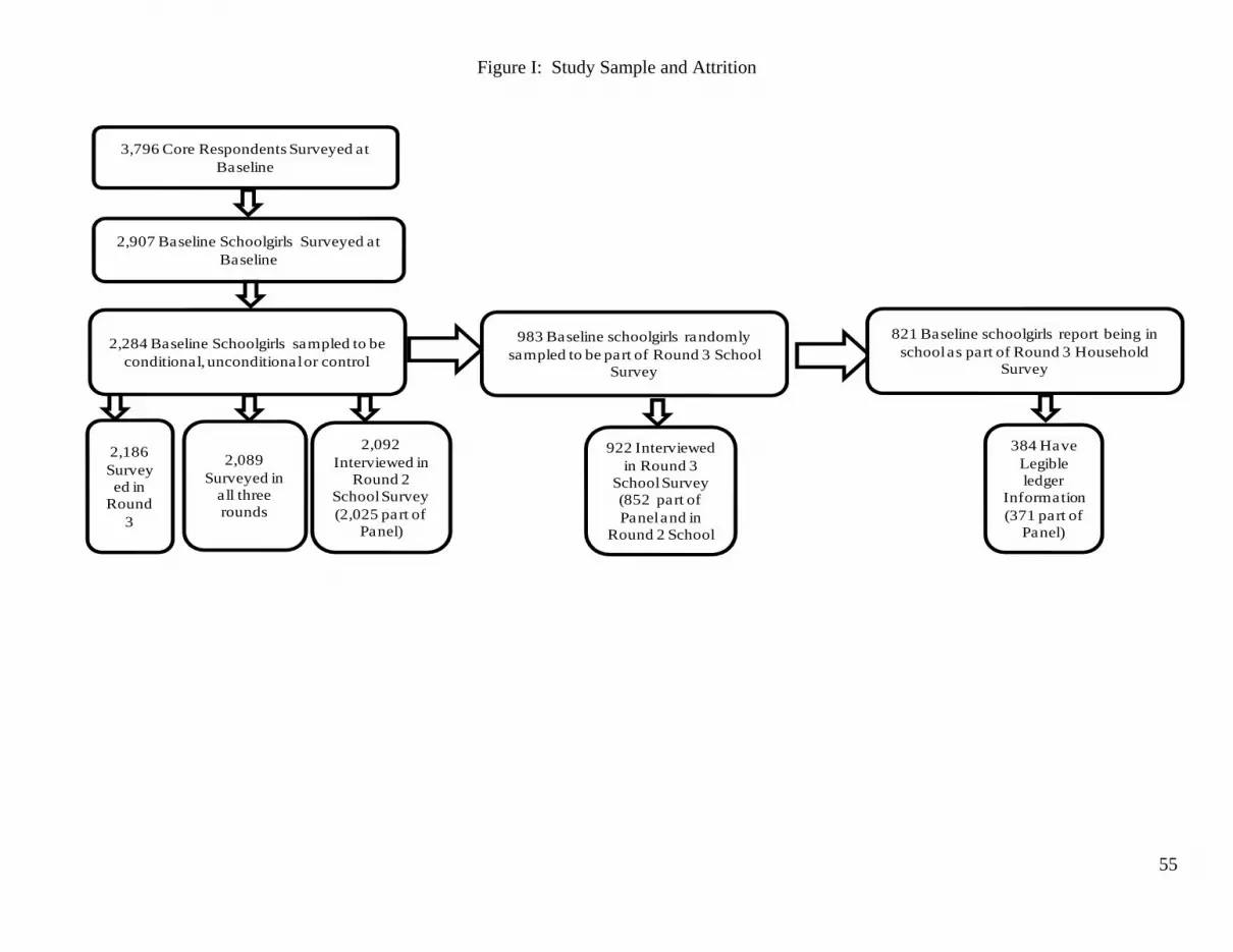
55

Figure I: Study Sample and Attrition

3,796 Core Respondents Surveyed at Baseline

2,907 Baseline Schoolgirls Surveyed at Baseline

2,284 Baseline Schoolgirls sampled to be conditional, unconditional or control

2,186 Surveyed in

Round 3

2,089 Surveyed in

all three rounds

2,092Interviewed in

Round 2 School Survey(2,025 part of

Panel)

983 Baseline schoolgirls randomly sampled to be part of Round 3 School

Survey

922 Interviewed in Round 3

School Survey(852 part of Panel and in

Round 2 School

821 Baseline schoolgirls report being in school as part of Round 3 Household

Survey

384 HaveLegible ledger

Information(371 part of

Panel)