arX

iv:1

211.

5893

v1 [

mat

h.N

A]

26

Nov

201

2

LOCAL BOUNDED COCHAIN PROJECTIONS

RICHARD S. FALK AND RAGNAR WINTHER

Abstract. We construct projections from HΛk(Ω), the space of differentialk forms on Ω which belong to L2(Ω) and whose exterior derivative also be-

longs to L2(Ω), to finite dimensional subspaces of HΛk(Ω) consisting of piece-

wise polynomial differential forms defined on a simplicial mesh of Ω. Thus,their definition requires less smoothness than assumed for the definition of thecanonical interpolants based on the degrees of freedom. Moreover, these pro-jections have the properties that they commute with the exterior derivativeand are bounded in the HΛk(Ω) norm independent of the mesh size h. Un-like some other recent work in this direction, the projections are also locallydefined in the sense that they are defined by local operators on overlappingmacroelements, in the spirit of the Clement interpolant.

1. Introduction

Projection operators which commute with the governing differential operatorsare key tools for the stability analysis of finite element methods associated to adifferential complex. In fact, such projections have been a central feature of theanalysis of mixed finite element methods since the beginning of such analysis, cf. [5,6]. However, a key difficulty is that, for most of the standard finite element spaces,the canonical projection operators defined from the degrees of freedom are not well–defined on the appropriate function spaces. This is the case for the Lagrange finiteelements, considered as a subspace of the Sobolev space H1, and for the Raviart-Thomas [18], Brezzi-Douglas-Marini [7], and Nedelec [16, 17] finite element spacesconsidered as subspaces ofH(div) orH(curl). For example, the classical continuouspiecewise linear interpolant, based on the values at the vertices of the mesh, is notdefined for functions in H1 in dimensions higher than one. Therefore, even if thecanonical projections commute with the governing differential operators on smoothfunctions, these operators cannot be directly used in a stability argument for theassociated finite element method due to the lack of boundedness of the projectionsin the proper operator norms. In addition to the canonical projection operators,it is worth mentioning another family of projection operators that commute withthe exterior derivative. This approach, usually referred to as projection basedinterpolation, is detailed in the work of Demkowicz and collaborators (cf. [8], [12],[13], [14], [15]). The main motivation for the construction of these operators was the

Date: November 19, 2012.2000 Mathematics Subject Classification. Primary: 65N30.Key words and phrases. cochain projections, finite element exterior calculus.The work of the first author was supported in part by NSF grant DMS-0910540. The work of

the second author was supported by the Norwegian Research Council.

1

2 RICHARD S. FALK AND RAGNAR WINTHER

analysis of the so called p–version of the finite element method, i.e., the focus is onthe dependence of the polynomial degree of the finite element spaces. However, asin the case of the canonical projection operators, the definition of these operatorsrequires some additional smoothness of the underlying functions, so again theycannot be used directly in the standard stability arguments. On the other hand,the classical Clement interpolant [11] is a local operator, and it is well–definedfor functions in L2. However, the Clement interpolant is not a projection, and theobvious extensions of the Clement operator to higher order finite element differentialforms (cf. [1, 3]) do not commute with the exterior derivative. Therefore, theseoperators are not directly suitable for a stability analysis.

Bounded commuting projections have been constructed in previous work. Thefirst such construction was given by Schoberl in [19]. The idea is to compose asmoothing operator and the unbounded canonical projection to obtain a boundedoperator which maps the proper function space into the finite element space. Inorder to obtain a projection, one composes the resulting operator with the inverseof this operator restricted to the finite element space. In [19], a perturbation ofthe finite element space itself was used to construct the proper smoother. In a re-lated paper, Christiansen [9] proposed to use a more standard smoothing operatordefined by a mollifier function. Using this idea, variants of Schoberl’s constructionare analyzed in [1, Section 5], [3, Section 5], and [10]. The constructed projectionscommute with the exterior derivative and they are bounded in L2. Therefore, theycan be used to establish stability of finite element methods. However, these projec-tions lack another key property of the canonical projections; they are not locallydefined. In fact, up to now it has been an open question if it is possible to constructbounded and commuting projections which are locally defined. The projections de-fined in this paper have all these properties. The construction presented belowresembles the construction of the Clement operator in the sense that it is based onlocal operators on overlapping macroelements.

We will adopt the language of finite element exterior calculus as in [1, 3]. Thetheory presented in these papers may be described as follows. Let Ω ⊂ R

n be abounded polyhedral domain, and let HΛk(Ω) be the space of differential k formsu on Ω, which is in L2, and where its exterior derivative, du = dku, is also in L2.This space is a Hilbert space. The L2 version of the de Rham complex then takesthe form

HΛ0(Ω)d−→ HΛ1(Ω)

d−→ · · ·

d−→ HΛn(Ω).

The basic construction in finite element exterior calculus is of a correspondingsubcomplex

Λ0h

d−→ Λ1

hd−→ · · ·

d−→ Λn

h,

where the spaces Λkh are finite dimensional subspaces of HΛk(Ω) consisting of piece-

wise polynomial differential forms with respect to a partition, Th, of the domain Ω.In the theoretical analysis of the stability of numerical methods constructed fromthis discrete complex, bounded projections πk

h : HΛk(Ω) → Λkh are utilized, such

LOCAL BOUNDED COCHAIN PROJECTIONS 3

that the diagram

HΛ0(Ω)d

−−→ HΛ1(Ω)d

−−→ · · ·d

−−→ HΛn(Ω)yπ0

h

yπ1h

yπnh

Λ0h

d−−→ Λ1

hd

−−→ · · ·d

−−→ Λnh

commutes. Such commuting projections are referred to as cochain projections. Theimportance of bounded cochain projections is immediately seen from the analysisof the mixed finite element approximation of the associated Hodge Laplacian. Infact, it follows from the results of [3, Section 3.3] that the existence of boundedcochain projections is equivalent to stability of the associated finite element method.Furthermore, if these projections are local, like the ones we construct here, thenimproved properties with respect to error estimates and adaptivity may be obtained.

For a general reference to finite element exterior calculus, we refer to the surveypapers [1, 3], and references given therein. As is shown there, the spaces Λk

h aretaken from two main families. Either Λk

h is of the form PrΛk(Th), consisting of

all elements of HΛk(Ω) which restrict to polynomial k-forms of degree at most ron each simplex T in the partition Th, or Λ

kh = P−

r Λk(Th), which is a space whichsits between PrΛ

k(Th) and Pr−1Λk(Th) (the exact definition will be recalled below).

These spaces are generalizations of the Raviart-Thomas and Brezzi-Douglas-Marinispaces, used to discretize H(div) and H(rot) in two space dimensions, and theNedelec edge and face spaces of the first and second kind, used to discretize H(curl)and H(div) in three space dimensions.

A main feature of the construction of the projections given below is that theyare based on a direct sum geometrical decomposition of the finite element space.In the general case of finite element differential forms, such a decomposition wasconstructed in [2]. However, this is a standard concept in the case of Lagrange finiteelements. Let Th be a simplicial triangulation of a polyhedral domain Ω ∈ R

n. IfT is a simplex we let ∆(T ) be the set of all subsimplexes of T , and by ∆m(T ) allsubsimplexes of dimension m. So if T is a tetrahedron in R

3, then ∆m(T ) are theset of vertices, edges, and faces of T for m = 0, 1, 2, respectively. We further denoteby ∆(Th) the set of all subsimplices of all dimensions of the triangulation Th, andcorrespondingly by ∆m(Th) the set of all subsimplices of dimension m. The desiredgeometric decomposition of the spaces PrΛ

k(Th) and P−r Λk(Th) is based on the

property that the elements of these spaces are uniquely determined by their trace,trf , for all f of ∆(Th) with dimension greater or equal to k. The decompositionsof the spaces PrΛ

k(Th) established in [2], is then of the form

(1.1) PrΛk(Th) =

⊕

f∈∆(Th)

dim f≥k

Ekf,r(PrΛ

k(f)).

Here PrΛk(f)) is the subspace of PrΛ

k(f)) consisting of elements with vanishing

trace on the boundary of f . The operator Ekf,r : PrΛ

k(f) → PrΛk(Th) is an exten-

sion operator in the sense that trf Ekf,r is the identity operator on PrΛ

k(f)). Fur-

thermore, Ekf,r is local in the sense that the support of functions in Ek

f,r(PrΛk(f))

is restricted to the union of the elements of Th which have f as a subsimplex. A

4 RICHARD S. FALK AND RAGNAR WINTHER

completely analog decomposition

(1.2) P−r Λk(Th) =

⊕

f∈∆(Th)

dim f≥k

Ek−f,r (P

−r Λk(f))

exists for the space P−r Λk(Th).

We will utilize modifications of the decompositions (1.1) and (1.2) to constructlocal bounded cochain projections onto the finite element spaces PrΛ

k(Th) andP−r Λk(Th). In the spirit of the Clement operator we will use local projections to

define the operators trf πkh for each f ∈ ∆(Th) with dimension greater or equal to

k. To make sure that the projections πkh commute with the exterior derivative we

will use a local Hodge Laplace problem to define the local projections, while theextension operators will be of the form of harmonic extension operators.

This paper is organized as follows. In Section 2 we introduce some basic notation,and we show how to construct the new projection in the case of scalar valuedfunctions, or zero forms. We also review some basic results on differential formsand their finite element approximations. A key step of the theory below is toconstruct a special projection into the space of Whitney forms [20], i.e., the spaceP−1 Λk(Th). In fact, in the present setting the construction in this lowest order

case is in some sense the most difficult part of the theory, since here we need torelate local operators defined on different subdomains. To achieve this we utilize astructure which resembles the Cech-de Rham double complex, cf. [4]. In additionto being a projection onto the Whitney forms, the special projection constructedin Section 3 will also satisfy a mean value property with respect to higher orderfinite element spaces, cf. equation (3.1) below. The general construction of thecochain projections, covering all spaces of the form PrΛ

k(Th) or P−r Λk(Th), is then

performed in Section 4. Finally, in Section 5 we derive precise local bounds for theconstructed projections.

2. Notation and preliminaries

We will use 〈·, ·〉 to denote L2 inner products on the domain Ω. For subdomainsD ⊂ Ω we will use a subscript to indicate the domain, i.e., we write 〈u, v〉D todenote L2 inner product on the domain D.

We will assume that Th is a family of simplicial triangulations of Ω ∈ Rn,

indexed by the mesh parameter h = maxT∈ThhT , where hT is the diameter of

T . In fact, hf will be used to denote the diameter of any f ∈ ∆(Th). We willassume throughout that the triangulation is shape regular, i.e. the ratio hn

T /|T |is uniformly bounded for all the simplices T ∈ Th and all triangulations of thefamily. Here |T | denotes the volume of T . Note that it is a simple consequence ofshape regularity that the ratio hT /hf , for f ∈ ∆(T ) with dim f ≥ 1 is also uniformlybounded. We will use [x0, x1, . . . xk] to denote the convex combination of the pointsx0, x1, . . . , xk ∈ Ω. Hence, any f ∈ ∆k(Th) is of the form f = [x0, x1, . . . xk],where x0, x1, . . . , xk ∈ ∆0(Th). Furthermore, the order of the points xj reflects theorientation of the manifold f . We will let fj ∈ ∆k−1(Th) denote the subcomplex off obtained by deleting the vertex xj , i.e., fj = [x0, . . . , xj−1, xj , xj+1, · · ·xk]. Here

LOCAL BOUNDED COCHAIN PROJECTIONS 5

the symbol over a term means that the term is omitted. Hence, if j is even thenfj has the orientation induced from f , while if the orientation is reversed if j isodd.

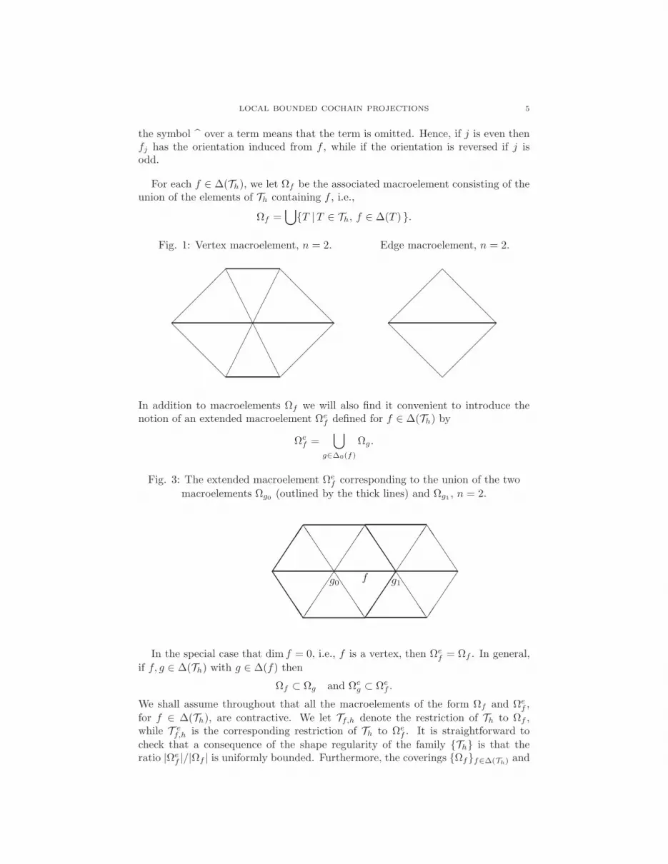
For each f ∈ ∆(Th), we let Ωf be the associated macroelement consisting of theunion of the elements of Th containing f , i.e.,

Ωf =⋃

T |T ∈ Th, f ∈ ∆(T ) .

Fig. 1: Vertex macroelement, n = 2. Edge macroelement, n = 2.

In addition to macroelements Ωf we will also find it convenient to introduce thenotion of an extended macroelement Ωe

f defined for f ∈ ∆(Th) by

Ωef =

⋃

g∈∆0(f)

Ωg.

Fig. 3: The extended macroelement Ωef corresponding to the union of the two

macroelements Ωg0 (outlined by the thick lines) and Ωg1 , n = 2.

fg0 g1

In the special case that dim f = 0, i.e., f is a vertex, then Ωef = Ωf . In general,

if f, g ∈ ∆(Th) with g ∈ ∆(f) then

Ωf ⊂ Ωg and Ωeg ⊂ Ωe

f .

We shall assume throughout that all the macroelements of the form Ωf and Ωef ,

for f ∈ ∆(Th), are contractive. We let Tf,h denote the restriction of Th to Ωf ,while T e

f,h is the corresponding restriction of Th to Ωef . It is straightforward to

check that a consequence of the shape regularity of the family Th is that theratio |Ωe

f |/|Ωf | is uniformly bounded. Furthermore, the coverings Ωff∈∆(Th) and

6 RICHARD S. FALK AND RAGNAR WINTHER

Ωeff∈∆(Th) of the domain Ω both have the bounded overlap property, i.e., the

sum of the characteristic functions is bounded uniformly in h.

2.1. Construction of the projection for scalar valued functions. To mo-tivate the construction for the general case of k forms given below, we will firstgive an outline of how the projection is constructed for zero forms, i.e. for scalarvalued functions. The projection π0

h will map the space H1(Ω) = HΛ0(Ω) intoPrΛ

0(Th), the space of continuous piecewise polynomials of degree r with respectto the partition Th. The space PrΛ

0(Tf,h) is the restriction of the space PrΛ0(Th)

to Tf,h, and PrΛ0(Tf,h) is the subspace of PrΛ

0(Tf,h) of functions which vanish on

the boundary of Ωf , ∂Ωf . Of course, by the zero extension the space PrΛ0(Tf,h)

can also be considered as a subspace of PrΛ0(Th).

A key tool for the construction is the local projection P 0f : H1(Ωf ) → Pr(Tf,h),

associated to each f ∈ ∆(Th). If dim f = 0, such that f is a vertex, we define P 0f

by P 0f u ∈ PrΛ

0(Tf,h) as the H1 projection of u, i.e., P 0f u is the solution of:

〈P 0f u, 1〉Ωf

= 〈u, 1〉Ωf,

〈dP 0f u, dv〉Ωf

= 〈du, dv〉Ωf, v ∈ Pr(Tf,h).

Of course, for zero forms the exterior derivative, d, can be identified with theordinary gradient operator. When 1 ≤ dim f ≤ n, we first define the space

PrΛ0(Tf,h) = u ∈ PrΛ

0(Tf,h) | trf u ∈ Pr(f) .

We then define P 0f u ∈ PrΛ

0(Tf,h) as the solution of

〈dP 0f u, dv〉Ωf

= 〈du, dv〉Ωf, v ∈ PrΛ

0(Tf,h).

The projection π0h will be defined recursively with respect to the dimensions of the

subsimplices of the triangulation Th. More precisely, we will utilize a sequence oflocal operators π0

m,hnm=0, and define π0

h = π0n,h. Dropping the dependence on h,

the operators π0m are defined recursively by

(2.1) π0mu = π0

m−1u+∑

f∈∆m(Th)

E0f trf P

0f (u − π0

m−1u), 1 ≤ m ≤ n.

Here E0f : Pr(f) → PrΛ

0(Tf,h) ⊂ PrΛ0(Th) is the harmonic extension operator

determined by

〈dE0fφ, dv〉Ωf

= 0, v ∈ PrΛ0(Tf,h), trf v = 0,

and that trf E0f is the identity on Pr(f). We observe that the dependency of the

operator E0f on the degree r is suppressed. It is a key property that trg E

0fφ = 0

for all g ∈ ∆(Th), dim g ≤ dim f , and g 6= f . For the vertex degrees of freedom wewill use an alternative extension operator. We simply define π0

0,h = π00 by

π00u =

∑

f∈∆0(Th)

E0f trf P

0f u =

∑

f∈∆0(Th)

E0f (P

0f u)(f)

where, for any α ∈ R, E0fα is the piecewise linear function with value α at the vertex

f and value zero at all other vertices. Hence, for f ∈ ∆0(Th) we have E0f = E0

f

if r = 1. The reason for choosing the special low order extension operator for

LOCAL BOUNDED COCHAIN PROJECTIONS 7

vertices is not essential at this point, but will be needed later to make sure that theprojections πk

h commute with the exterior derivative.

The key result for the construction above is that the operator π0h is a projection.

Lemma 2.1. The operator π0h is a projection onto PrΛ

0(Th).

Proof. To see that π0 = π0h is a projection, we only need to check that if u ∈

PrΛ0(Th), then for all f ∈ ∆(Th), trf π

0u = trf u. We do this by induction onm, where m corresponds to the dimension of the face f ∈ ∆(Th). We assumethroughout that u ∈ PrΛ

0(Th). We will show that the operator π0m has the property

that

(2.2) trf π0mu = trf u if f ∈ ∆(Th) with dim f ≤ m,

and since π0 = π0n this will establish the desired result. If f ∈ ∆0(Th) then P 0

hu =u|Ωf

. By construction, it therefore follows that (2.2) holds for m = 0. Assume nextthat (2.2) holds for m−1, where 1 ≤ m ≤ n. It follows that for any f ∈ ∆m(Th) we

have trf (u−π0m−1u) ∈ Pr(f), and therefore P 0

f (u−π0m−1u) = u−π0

m−1u. It follows

by construction that trg π0mu = trg π

0m−1u = trg u for g ∈ ∆(Th), with dim g < m,

while for f ∈ ∆m(Th) we have

trf π0mu = trf (π

0m−1u+ P 0

f (u− π0m−1u) = trf u.

Therefore, (2.2) holds for m and the proof is completed.

It follows from the construction above that the operator π0h is local. For example,

for any T ∈ Th we have that (π00,hu)T depends only on u restricted to the extended

macroelement ΩeT . Define Dm,T ⊂ Ω by

(2.3) Dm,T = ∪Dm−1,T ′ |T ′ ∈ Tf,h, f ∈ ∆m(T ) , D0,T = ΩeT .

It follows from (2.1) that (πm,hu)|T depends only on u|Dm,T. In particular, (π0

hu)|Tdepends only on u|DT

, where DT = Dn,T .

The operator π0h satisfies the following local estimate.

Theorem 2.2. Let T ∈ Th. The operator π0h satisfies the bounds

‖π0hu‖L2(T ) ≤ C(‖u‖L2(DT ) + hT ‖du‖L2(DT ))

and

‖dπ0hu‖L2(T ) ≤ C‖du‖L2(DT ),

where the constant C is independent of h and T ∈ Th.

In fact, this result is just a special case of Theorem 5.2 below, so we omit the proofhere. Of course, due to the bounded overlap property of the covering DT T∈Th

of Ω, derived from the corresponding property of Ωef, global estimates follow

directly from the local estimates above.

8 RICHARD S. FALK AND RAGNAR WINTHER

2.2. Differential forms and finite element spaces. We will basically adoptthe notation from [3]. The spaces PrΛ

k(Th) ⊂ HΛk(Ω) can be characterized as thespace of piecewise polynomial k forms u of degree less than or equal to r, such thatthe trace, trf u, is continuous for all f ∈ ∆(Th), with dim f ≥ k, where we recall thatthe trace, trf , of a differential form is defined by restricting to f and applying theform only to tangent vectors. The space P−

r Λk(Th) ⊂ HΛk(Ω) is defined similarly,but on each element T ∈ Th, u is restricted to be in P−

r Λk ⊂ PrΛk. Here, the

polynomial class P−r Λk consists of all elements u of PrΛ

k such that u contractedwith the position vector x, uyx, is in PrΛ

k−1. Hence, for each k we have a sequenceof nested spaces

P−1 Λk(Th) ⊂ P1Λ

k(Th) ⊂ P−2 Λk(Th) ⊂ . . . HΛk(Ω).

In particular, P−r Λ0(Th) = PrΛ

0(Th), and P−r Λn(Th) = Pr−1Λ

n(Th).

Instead of distinguishing the theory for the spaces P−r Λk(Th) and PrΛ

k(Th) wewill use the simplified notation PΛk(Th) to denote either a space of the familyP−r Λk(Th) or PrΛ

k(Th). More precisely, we assume that we are given a sequenceof spaces PΛk(Th), for k = 0, 1, . . . , n, such that the corresponding polynomialsequence (PΛ, d), given by

(2.4) R → PΛ0(Rn)d

−−→ PΛ1(Rn)d

−−→ · · ·d

−−→ PΛn(Rn) → 0

is an exact complex (cf. Section 5.1.4 of [3]). In particular, this allows for combi-nations of spaces taken from the two families P−

r Λk(Th) and PrΛk(Th). For any

f ∈ ∆(T ), with dim f ≥ k, the space PΛk(f) = trf PΛk(Th), while PΛk(f) =v ∈ PΛk(f) | tr∂f v = 0. The corresponding polynomial complexes of the form(PΛ(f), d) are all exact. Furthermore, the complexes with homogeneous boundary

conditions, (PΛ(f), d), given by

(2.5) PΛ0(f)d

−−→ PΛ1(f)d

−−→ · · ·d

−−→ PΛdimf (f) → R

are also exact.

We recall that the spaces PΛk(Th) admit degrees of freedom of the form

(2.6)

∫

f

trf u ∧ η, η ∈ P ′(f, k), f ∈ ∆(Th),

where P ′(f, k) ⊂ Λdimf−k(f) is a polynomial space of differential forms and thesymbol ∧ is used to denote the exterior product. These degrees of freedom uniquelydetermine an element in PΛk(Th), (cf. Theorem 5.5 of [3]). In fact, if

PΛk(Th) = P−r Λk(Th), then P ′(f, k) = Pr+k−dim f−1Λ

dim f−k(f),

while if

PΛk(Th) = PrΛk(Th), then P ′(f, k) = P−

r+k−dim fΛdim f−k(f).

If v ∈ PΛk(f), then v is uniquely determined by the functionals derived fromP ′(f, k). Furthermore, any v ∈ PΛk(f) is uniquely determined by P ′(g, k) for allg ∈ ∆(f). In particular, if dim f < k then P ′(f, k) is empty, while P ′(f, k) is alwaysnonempty if dim f = k. For dim f > k the set P ′(f, k) can also be empty if thepolynomial degree r is sufficiently low.

LOCAL BOUNDED COCHAIN PROJECTIONS 9

The local spaces PΛk(Tf,h) and PΛk(T ef,h) are defined by restricting the space

PΛk(Th) to the macroelements Ωf or Ωef . It follows from the assumption that Ωf

and Ωef are contractive, that all the local complexes (PΛ(Tf,h), d) and (PΛ(T e

f,h), d)

are exact. The same holds for the subcomplexes (PΛ(Tf,h), d) and (PΛ(T ef,h), d),

corresponding to the subspaces of functions with zero trace on the boundary of themacroelements.

For a given triangulation Th, the spaces of lowest order polynomial degree,P−1 Λk(Th), i.e., the space of Whitney forms, will play a special role in our construc-

tion. The dimension of this space is equal to the number of elements in ∆k(Th),and the properties of these spaces will in some sense reflect the properties of thetriangulation. Therefore, this space will be used to transfer information betweendifferent macroelements, cf. Section 3 below. For k = 0 this space is just P1Λ

k(Th),the space of continuous piecewise linear functions. The natural basis for this spaceis the set of generalized barycentric coordinates, defined to be one at one vertex,and zero at all other vertices. It follows from the discussion above that the degreesof freedom for the space P−

1 Λk(Th), 0 ≤ k ≤ n, are∫f u for all f ∈ ∆k(Th). In

fact, if f = [x0, x1, . . . xk] ∈ ∆k(Th), we define the Whitney form associated to f ,φkf ∈ P−

1 Λk(Th), by

φkf =

k∑

i=0

(−1)iλidλ0 ∧ · · · ∧ dλi ∧ · · · ∧ dλk,

where λ0, λ1, . . . , λk are the barycentric coordinates associated to the vertices xi.The basis function φk

f reduces to a constant k form on f , i.e., trf φkf ∈ P0Λ

k(f), and

it has the property that trg φkf = 0 for g ∈ ∆k(Th), g 6= f . In fact, if volf ∈ P0Λ

k(f)

is the volume form on f , scaled such that∫fvolf = 1, then

trf φkf = (k!)−1

volf ,

cf. [1, Section 4.1]. Furthermore, the map volf → Ekf volf = k!φk

f defines an

extension operator Ekf : P0Λ

k(f) → P−1 Λk(Tf,h) for any f ∈ ∆k(Th). We observe

that the operators Ekf are natural generalizations of the piecewise linear extension

operators E0f , introduced above for scalar valued functions. In fact, any element u

of P−1 Λk(Th) admits the representation

(2.7) u =∑

f∈∆k(Th)

(∫

f

trf u

)Ekf volf .

We finally note that it follows from Stokes’ theorem that if f = [x0, x1, . . . , xk+1],and u is a sufficiently smooth k form on f , then

(2.8)

∫

f

du =

k+1∑

j=0

(−1)j∫

fj

trfj u,

where fj = [x0, . . . , xj−1, xj , xj+1, · · ·xk+1]. Here the factor (−1)j enters as aconsequence of orientation.

10 RICHARD S. FALK AND RAGNAR WINTHER

3. A special projection onto the Whitney forms

Recall that the purpose of this paper is to construct local cochain projectionsπkh which map HΛk(Ω) boundedly onto the piecewise polynomial space PΛk(Th).

Furthermore, in the construction of π0h given above, the construction of trf π

0h is

based on a local projection, P 0f , defined with respect to the associated macroelement

Ωf . Therefore one might hope that all the projections πkh have the property that

trf πkh is defined from a local projection operator defined on Ωf for f ∈ ∆(Th),

dim f ≥ k. However, a simple computation in two space dimensions, and withPΛk(Th) = P−

1 Λk(Th), will convince the reader that if f = [x0, x1] ∈ ∆1(Th), then∫

f

trf dπ0hu =

∫ x1

x0

d

dsπ0hu ds = (π0

hu)(x1)− (π0hu)(x0),

and the right hand side here clearly depends on u restricted to the union of themacroelements associated to the vertices x0 and x1. Therefore,

∫ftrf π

h1du =∫

f trf dπ0hu must also depend on u restricted to the union of these macroelements,

and this domain is exactly equal to the extended macroelement Ωef . This motivates

why the extended macroelements, Ωef , for f ∈ ∆k(Th), will appear in the construc-

tion below. In fact, a special projection operator, Rkh : HΛk(Ω) → P−

1 Λk(Th) ⊂PΛk(Th), will be utilized in the construction of πk

h to make sure that∫

f

trf πkhdu =

∫

f

trf dπk−1h u =

∫

∂f

tr∂f πk−1h u,

for all f ∈ ∆k(Th).

The operator Rkh will commute with the exterior derivative, and it is a projec-

tion onto P−1 Λk(Th). Therefore, in the case of lowest polynomial degree, when

PΛk(Th) = P−1 Λk(Th), we will take πk

h = Rkh. However, another key property of

the operator Rkh is that in the general case, when P−

1 Λk(Th) is only contained inPΛk(Th), we will have

(3.1)

∫

f

trf Rkhu =

∫

f

trf u, f ∈ ∆k(Th), u ∈ PΛk(Th),

i.e., the operator Rkh preserves the mean values of the traces of function in PΛk(Th)

on subsimplexes f of dimension k. The rest of this section is devoted to the con-struction of the operator Rk

h, and the derivation of the key properties given inTheorem 3.6 below.

3.1. Tools for the construction. Throughout this section the dependence onthe mesh parameter h is suppressed in order to simplify the notation. To definethe special projection Rk onto the Whitney forms, P−

1 Λk(T ), we will use localprojections, Qk

f , defined with respect to the extended macroelements Ωef . We define

the projection Qkf : HΛk(Ωe

f ) → PΛk(T ef ) by the system

〈Qkfu, dτ〉Ωe

f= 〈u, dτ〉Ωe

f, τ ∈ PΛk−1(T e

f ),

〈dQkfu, dv〉Ωe

f= 〈du, dv〉Ωe

f, v ∈ PΛk(T e

f ).

LOCAL BOUNDED COCHAIN PROJECTIONS 11

For k = 0, the first equation should be replaced by a mean value condition, so thatQ0

f = P 0f . This system has a unique solution due to the exactness of the complex

(PΛ(T ef ), d). Furthermore, by construction we have

(3.2) Qkfdu = dQk−1

f u, 0 < k ≤ n.

We will also find it useful to introduce the operator Qkf,− : HΛk(Ωe

f ) → PΛk−1(T ef )

defined by the corresponding reduced system

〈Qkf,−u, dτ〉Ωe

f= 0, τ ∈ PΛk−2(T e

f,h),

〈dQkf,−u, dv〉Ωe

f= 〈u, dv〉Ωe

f, v ∈ PΛk−1(T e

f,h).

As a consequence, the projection Qkf can be expressed as

(3.3) Qkf = dQk

f,− +Qk+1f,− d.

To make this relation true also in the case when k = 0 and f ∈ ∆0(T ), the operatordQ0

f,− should have the interpretation that dQ0f,−u is the constant

∫Ωf

u ∧ volΩfon

Ωf , where volΩfis the volume form on Ω, restricted to Ωf and scaled such that∫

ΩfvolΩf

= 1.

To motivate the rest of the tools we need to for our construction, consider againdπ0u in the special case when PΛk(T ) = P−

1 Λk(T ). To obtain a commutingrelation of the form dπ0u = π1du, we have to be able to express dπ0u in termsof du. However, using the notation just introduced, we have

dπ0u =∑

g∈∆0(T )

[(∫

Ωg

u ∧ volΩg

)+ trg(Q

1g,−du)

]dEgvolg.

The second part of this sum is already expressed in terms of du. By combining thecontributions from neighbouring macroelements we wil see that also the first partof the right hand side can be expressed in term of du. If f = [x0, x1] ∈ ∆1(T ), wehave ∫

f

trf∑

g∈∆0(T )

( ∫

Ωg

u ∧ volΩg

)dEgvolg =

∫

Ωef

u ∧ (volΩg1− volΩg0

),

where gi = [xi]. Furthermore, volΩg1− volΩg0

∈ P0Λn(T e

f ) = P−1 Λn(T e

f ), and with

vanishing integral. As a consequence, there exists z1f ∈ P−1 Λn−1(T e

f ) such that

dz1f = volΩg0− volΩg1

, and by integration by parts∫

f

trf∑

g∈∆0(T )

( ∫

Ωg

u ∧ volΩg

)dEgvolg = −

∫

Ωef

u ∧ dz1f =

∫

Ωef

du ∧ z1f .

By utilizing the representation (2.7), we therefore obtain∑

g∈∆0(T )

( ∫

Ωg

u ∧ volΩg

)dEgvolg =

∑

f∈∆1(Th)

( ∫

Ωef

du ∧ z1f

)Ekf volf .

This discussion shows that to construct local cochain projections, we must utilizerelations between local operators defined on different macroelements. To derive theproper relations, we introduce an operator

δ :⊕

g∈∆m(T )

P−1 Λk(T e

g ) →⊕

f∈∆m+1(T )

P−1 Λk(T e

f ).

12 RICHARD S. FALK AND RAGNAR WINTHER

If f = [x0, . . . , xm+1] ∈ ∆m+1(T ), then the component (δu)f of δu is defined by

(δu)f =

m+1∑

j=0

(−1)jufj ,

where, as above, fj = [x0, . . . , xj−1, xj , xj+1, · · ·xm+1], and ufj the correspondingcomponent of u. We will also consider the exterior derivative d as an operatormapping

⊕g∈∆m(T ) P

−1 Λk(T e

g ) to⊕

g∈∆m(T ) P−1 Λk+1(T e

g ) by applying it to each

component. Hence, the two operators dδ and δd both map⊕

g∈∆m(T ) P−1 Λk(T e

g )

into⊕

f∈∆m+1(T ) P−1 Λk+1(T e

f ). In fact, we have the stucture of a double complex

which resembles the well–known Cech–de Rham complex, cf. [4]. The followingtwo properties of the operator δ are crucial.

Lemma 3.1.

d δ = δ d, and δ δ = 0.

Proof. It follows directly from the definition of δ that for f = [x0, . . . , xm+1] ∈∆m+1(T )

(d δu)f = (δ du)f =

m+1∑

j=0

(−1)jdufj .

If we further denote by fij the subsimplex of f obtained by deleting both xi andxj , then

(δ δu)f =

m+1∑

j=0

(−1)j(δu)fj

=

m+1∑

j=0

(−1)j[ j−1∑

i=0

(−1)iufij −

m+1∑

i=j+1

(−1)iufij

]= 0,

since for each i, j = 0, . . .m + 1, with i 6= j, the term ufij appears exactly twicewith opposite signs.

The construction of the projection Rk = Rkh will depend on local weight func-

tions, zkf ∈ P−1 Λn−k(T e

f ) for f ∈ ∆k(T ). In particular, the function z0f ∈ P0Λn(Tf )

for f ∈ ∆0(T ) will be given by z0f = volΩf. For k = 1, 2, . . . , n, the functions

zkf ∈ P−1 Λn−k(T e

f ) are defined recursively to satisfy the conditions

(3.4) dzkf = (−1)k(δzk−1)f ,

and

(3.5) 〈zkf , dτ〉Ωef= 0, τ ∈ P−

1 Λn−k−1(T ef ),

for any f ∈ ∆k(T ). We will not give an explicit construction of the functions zkf .However, we have the following basic result.

Lemma 3.2. The weight functions zkf ∈ P−1 Λn−k(T e

f ) exist and are uniquely de-

termined by z0f and the conditions (3.4) and (3.5).

LOCAL BOUNDED COCHAIN PROJECTIONS 13

Proof. We establish the existence of the functions zkf by induction on k. Let f =

[x0, x1] ∈ ∆1(T ). Then

(δz0)f = (z0f1 − z0f0) = volΩf1− volΩf0

,

which implies that∫Ωe

f

(δz0)f = 0. Hence, by the exactness of the complex

P−1 Λn−1(T e

f )d−→ P0Λ

n(T ef ) → R,

there exists z1f ∈ P−1 Λn−1(T e

f ) satisfying dz1f = −(δz0)f . Next, assume we have con-

structed zk−1 ∈⊕

f∈∆k−1(T ) P−1 Λn−k+1(T e

f ) such that dzk−1f = (−1)k−1(δzk−2)f

for all f ∈ ∆k−1(T ). From Lemma 3.1 we obtain

(d δ)zk−1 = (δ d)zk−1 = (−1)k−1(δ δ)zk−2 = 0,

and for each f ∈ ∆k(T ) the complex (d, P−1 Λ(T e

f )) is exact. Therefore, we can

conclude that there is a zkf ∈ P−1 Λn−k(∆k(T

ef )) such that (3.4) holds. This com-

pletes the induction argument. Finally, we observe that it is a consequence of (3.5)

and the exactness of the complex (d, P−1 Λ(T e

f )) that each function zkf is uniquelydetermined.

We will use the functions zkf to define an operator Mk := Mkh : HΛk(Ω) →

P−1 Λk(T ) by

Mku =∑

f∈∆k(T )

(∫

Ωef

u ∧ zkf

)Ekf volf .

Note that Mku is a generalization for k-forms of the expression

∑

f∈∆0(T )

( ∫

Ωf

u ∧ volΩf

)Efvolf .

appearing above in the case of zero-forms. It follows from the construction of thefunctions zkf that the operator Mk commutes with the exterior derivative.

Lemma 3.3. For any v ∈ HΛk−1(Ω) the identity dMk−1v = Mkdv holds.

Proof. We have to show that

∑

g∈∆k−1(T )

( ∫

Ωeg

v ∧ zk−1g

)dEk−1

g volg =∑

f∈∆k(T )

( ∫

Ωef

dv ∧ zkf

)Ekf volf

for any v ∈ HΛk−1(Ω). Since both sides of this equation are elements of P−1 Λk(T ),

we need only check that the integrals of their traces are the same over each f =[x0.x1, . . . , xk] ∈ ∆k(T ). Now it follows from the properties of the extension oper-ators Ek

f that the integral of the right hand side is simply∫Ωe

f

dv ∧ zkf , while (2.8)

implies that the corresponding integral of the left hand side is

k∑

j=0

(−1)j∫

Ωefj

v ∧ zk−1fj

=

∫

Ωef

v ∧ (δzk−1)f = (−1)k∫

Ωef

v ∧ dzkf ,

14 RICHARD S. FALK AND RAGNAR WINTHER

where the last identity follows by (3.4). However, by integration by parts (cf. [1,Section 2.2]), utilizing that tr∂Ωe

fzkf = 0, we have

∫

Ωef

v ∧ dzkf = (−1)k∫

Ωef

dv ∧ zkf ,

and this completes the proof.

We now define an operator Sk = Skh : HΛk(Ω) → P−

1 Λk(T ) recursively byS0 = M0 and

Sku = Mku+∑

g∈∆k−1(T )

(∫

g

trg[I − Sk−1]Qkg,−u

)dEk−1

g volg, 1 ≤ k ≤ n.

We recall that the operator Qkg,− is a local operator with range PΛ(T e

f ). However,

by an inductive argument, it follows that the composition trf Sk is a local operator

mapping HΛk(Ωef ) into P0Λ

k(f). Therefore, the operators Sk are indeed welldefined.

A key property of the operator Sk is the following result.

Lemma 3.4. For any v ∈ PΛk−1(T ) the identity∫

f

Skdv =

∫

f

dv, f ∈ ∆k(T ).

holds.

Proof. The proof goes by induction on k. For k = 0 the space dPΛk−1(T ) should beinterpreted as the space of constants on Ω, and since S0 = M0 reproduces constantsthe desired identity holds.

Assume next that k ≥ 1 and that the desired identity holds for k − 1. Byutilizing the result of Lemma 3.3 we obtain that the commutator Skd− dSk−1 hasthe representation

Skdv− dSk−1v =∑

g∈∆k−1(T )

(∫

g

trg[I −Sk−1]Qkg,−dv

)dEk−1

g volg, v ∈ HΛk−1(Ω).

We recall thatQkg,−dv = Qk−1

g v−dQk−1g,− v, and by the induction hypothesis

∫gtrg(I−

Sk−1)dQk−1g,− v = 0. Therefore, for any v ∈ HΛk−1(Ω) the commutator above can

be expressed as

(3.6) Skdv − dSk−1v =∑

g∈∆k−1(T )

( ∫

g

trg[I − Sk−1]Qk−1g v

)dEk−1

g volg.

However, since Qk−1g is a projection onto PΛk−1(T e

g ), it follows from (2.7) that

dSk−1v =∑

g∈∆k−1(T )

( ∫

g

trg Sk−1Qk−1

g v)dEk−1

g volg, v ∈ PΛk−1(T ).

By restricting to a function v ∈ PΛk−1(T ) equation (3.6) therefore reduces to

Skdv =∑

g∈∆k−1(T )

(∫

g

trg v)dEk−1

g volg.

LOCAL BOUNDED COCHAIN PROJECTIONS 15

By integrating this representation over any f = [x0, x1, . . . , xk] ∈ ∆k(T ) we obtain

∫

f

Skdv =

k∑

j=0

(−1)j∫

fj

trfj v =

∫

f

dv,

where the final identity follows from (2.8) This completes the induction argument.

As a direct consequence of the proof above, we have.

Lemma 3.5. The identity (3.6) holds for k = 1, 2, . . . , n and all v ∈ HΛk−1(Ω).

3.2. The projection Rkh. For each k, 0 ≤ k ≤ n, the operator Rk = Rk

h :HΛk(Ω) → P−

1 Λk(T ) is defined by

Rku = Sku+∑

f∈∆k(T )

( ∫

f

trf [I − Sk]Qkfu)Ekf volf .

Recall that the operator Sk is local in the sense that trf Sk can be seen as a

local operator mapping HΛk(Ωef ) onto PΛk(f). It is immediate from this and

the properties of of the projection Qkf , that trf R

k also is local. In fact, for any

T ∈ T , (Rku)|T only depends on u|ΩeT. Furthermore, if f ∈ ∆0(Th) then Q0

f = P 0f .

Therefore, it follows that for k = 0 the operator R0h is identical to the operator

π00,h, used in the construction of the projection π0

h in Section 2.1 above.

The key properties of the operator Rkh are given in the theorem below.

Theorem 3.6. The operators Rkh : HΛk(Ω) → P−

1 Λk(Th) are cochain projections.

Furthermore, they satisfy property (3.1), i.e.,∫

f

trf Rkhu =

∫

f

trf u, f ∈ ∆k(Th), u ∈ PΛk(Th).

Proof. As above we use a notation where we suppress the dependence on h. It isa consequence of the projection property of the operators Qk

f that if u ∈ PΛk(T )then

Rku =∑

f∈∆k(T )

(∫

f

trf u)Ekf volf .

However, this implies the identity (3.1), and an immediate further consequence isthat Rk is a projection onto P−

1 Λk(Th).

It remains to show that Rk commutes with the exterior derivative. From thedefinition of Rk and Lemma 3.5 we have

dRku = dSku+∑

f∈∆k(T )

(∫

f

trf [I − Sk]Qkfu)dEk

f volf = Sk+1du.

However, Sk+1du = Rk+1du since

Rk+1du − Sk+1du =∑

f∈∆k+1(T )

(∫

f

trf [I − Sk+1]Qk+1f du

)Ek+1f volf

16 RICHARD S. FALK AND RAGNAR WINTHER

=∑

f∈∆k+1(T )

(∫

f

trf [I − Sk+1]dQk+1f,− du

)Ek+1f volf = 0,

where the last identity follows from Lemma 3.4.

The operators Rkh introduced above are local operators in the sense that (Rk

hu)|Tonly depends on u|Ωe

Tfor any T ∈ Th. Furthermore, for any fixed h the operator

Rkh is a bounded operator on HΛk(Ω). The discussion of more precise local bounds

is delayed until the final section of the paper.

4. Construction of the Projection: The General Case

We finally turn to the construction of the projections πkh in the general case, in

which PΛk(Th) denotes any family of spaces of the form P−r Λk(Th) or PrΛ

k(Th),such that the corresponding polynomial sequence (PΛk, d), given by (2.4) is an exactcomplex. In particular, the Whitney forms, P−

1 Λk(Th), are a subset of PΛk(Th),and in the special case when PΛk(Th) = P−

1 Λk(Th) we will take πkh to be the

operator Rkh constructed above.

In the construction we will utilize a decomposition of PΛk(Th) of the form

(4.1) PΛk(Th) =⊕

f∈∆k(Th)

Ekf (P0Λ

k(f)) +⊕

f∈∆(Th)

dim f≥k

Ekf (PΛk(f)),

where Ekf is the extension operator defined in the previous section, mapping into

the space of Whitney forms, while Ekf is an harmonic extension operator mapping

into PΛk(Tf,h). Furthermore, the space PΛk(f) = PΛk(f) if dim f > k, while

PΛk(f) = u ∈ PΛk(f) |

∫

f

u = 0, if dim f = k.

The decomposition (4.1) can be seen a modification of the more standard decom-positions (1.1) and (1.2) in the sense that we are utilizing the special extension, Ek

f ,for the constant term of the traces on f , when dim f = k. The existence of such adecomposition of the space PΛk(Tf ) is an immediate consequence of the degrees offreedom (2.6).

As in the case k = 0, cf. Section 2.1, the projection πkh will be constructed from

a sequence of operators πkm,h, where πk

h = πkn,h. The operators πk

m,h are defined bya recursion of the form

(4.2) πkm,h = πk

m−1,h +∑

f∈∆m(Th)

Ekf trf P

kf [I − πk

m−1,h], k ≤ m ≤ n,

where the operators P kf are local projections defined with respect to the macroele-

ments Ωf , generalizing the operators P 0f introduced in Section 2.1. Furthermore,

the operator πkk−1,h will be taken to be the operator Rk

h defined in Section 3 above.

Hence, to complete the definition of πkh, it remains to give precise definitions of the

local operators Ekf and P k

f .

LOCAL BOUNDED COCHAIN PROJECTIONS 17

4.1. Extension operators. As above, to simplify the notation, we suppress thedependence on h throughout the discussion. The extension operators Ek

f are gener-

alizations of the harmonic extension operators E0f used for zero forms in Section 2.1.

Let us first assume that f ∈ ∆(T ) such that f is not a subset of the boundary of

Ωf . In this case, the harmonic extension Ekf maps PΛk(f) to PΛk(Tf ), where

0 ≤ k ≤ dim f . More specifically, we let Ekfφ be characterized by

‖dEkfφ‖L2(Ωf ) = inf‖dv‖L2(Ωf ) | v ∈ PΛk(Tf ), trf v = φ .

We should note that it is a consequence of the degrees of freedom of the spacesPΛk(Tf ) and PΛk(Tf ) that there are feasible solutions to this optimization problem.As a consequence, an optimal solution exists. However, the solution is in generalnot unique. The solution is only determined up to adding functions w in PΛk(Tf,h)satisfying dw = 0 on Ωf and trfw = 0. Therefore, to obtain a well defined extensionoperator, we need to introduce a corresponding gauge condition. Hence, for any

φ ∈ PΛk(f) we let Ekfφ ∈ PΛk(Tf ) be the solution of the system

(4.3)〈Ek

fφ, dτ〉Ωf= 0, τ ∈ N(trf ; PΛk−1(Tf )),

〈dEkfφ, dv〉Ωf

= 0, v ∈ N(trf ; PΛk(Tf )),

and such that trf Ekf is the identity on PΛk(f). Here N(trf ;X) denotes the

kernel of the operator trf restricted to the function space X . A key property of theextension operators Ek

f is that they commute with the exterior derivative.

Lemma 4.1. Let f ∈ ∆(T ). The extension operators Ekf : PΛk(f) → PΛk(Tf )

are well defined by the system (4.3) for k = 0, 1, . . . , dim f , and for k ≥ 1 we have

the identity

(4.4) Ekfdφ = dEk−1

f φ, φ ∈ PΛk−1(f).

Moreover, the kernel of d restricted to N(trf ; PΛk(Tf )) is dN(trf ; PΛk−1(Tf )).

Proof. For k = 0 the first equation in the system (4.3) should be omitted. The

kernel of d restricted to N(trf ; PΛ0(Tf )) is just the zero function, and E0fφ is

clearly uniquely determined by the second equation and the extension property.We proceed by induction on k.

Assume that the statement of the lemma holds for all levels less than k. Wefirst establish the characterization of the kernel of d, restricted to N(trf ; PΛk(Tf )).

Assume that u ∈ N(trf ; PΛk(Tf )) satisfies du = 0. Then, by the exactness of the

complex (PΛ(Tf ), d), u = dτ for some τ ∈ PΛk−1(Tf ). Furthermore, d trf τ =

trf dτ = trf u = 0. If k = 1 this implies that τ ∈ N(trf ; PΛ0(Tf )). For k > 1 it

follows from the exactness of (PΛ(f), d) that there is a φ ∈ PΛk−2(f) such thatdφ = trf τ . However, the function

σ = τ − dEk−2φ = τ − Ek−1dφ

∈ N(trf ; PΛk−1(Tf )) and satisfies dσ = u. Hence the complex (N(trf ; PΛ(Tf)), d)

is exact at level k in the sense that dN(trf ; PΛk−1(Tf )) is the kernel of d restricted

to N(trf ; PΛk(Tf )).

18 RICHARD S. FALK AND RAGNAR WINTHER

Consider a local Hodge Laplace problem of the form:

(4.5)〈σ, τ〉Ωf

− 〈u, dτ〉Ωf= 0, τ ∈ N(trf ; PΛk−1(Tf )),

〈dσ, v〉Ωf+ 〈du, dv〉Ωf

= 0, v ∈ N(trf ; PΛk(Tf )),

where the unknown (σ, u) ∈ N(trf ; PΛk−1(Tf )) × PΛk(Tf ), and with trf u = φ ∈

PΛk(f). Since the complex (N(trf ; PΛ(Tf )), d) is exact at level k, it follows fromthe abstract theory of Hodge Laplace problems, cf. for example [3, Section 3], thatthe system (4.5) has a unique solution. Furthermore, by the exactness of the samecomplex at level k − 1, σ = 0. Hence, u and Ek

fφ satisfy the same conditions, and

the uniqueness of Ekfφ follows by the uniqueness of u.

Finally, to show the identity (4.4) we just observe that for any φ ∈ PΛk−1(f),

the pair (σ, u), with σ = 0 and u = dEk−1f φ ∈ PΛ(Tf ), satisfies the system (4.5)

with trf dEk−1f φ = d trf E

k−1f φ = dφ. By uniqueness of such solutions we conclude

that dEk−1f φ = Ek

f dφ. This completes the induction argument, and the proof ofthe lemma.

If g ∈ ∆(Tf ), with k ≤ dim g ≤ dim f and g 6= f , then trg Ekfφ = 0. In the case

that f ⊂ ∂Ω, we will also have that f ⊂ ∂Ωf . In this case, the definition of theoperator Ek

f should be properly modified, such that Ekfφ is not required to be in

PΛk(Tf ), but only required to be zero on the interior part of ∂Ωf . The key desiredproperty is that the extension of Ek

fφ from Ωf to Ω, by zero outside Ωf , is in the

global space PΛk(Th).

It is a consequence of the decomposition (4.1) that any element u of PΛk(T )is uniquely determined by its trace on f , trf u, for all f ∈ ∆(T ) with dim f ≥ k.Furthermore, if u is an element of the subspace given by

(4.6)⊕

f∈∆k(T )

Ekf (P0Λ

k(f)) +⊕

f∈∆(T )

k≤dim f≤m

Ekf (PΛk(f)),

then u is determined by trf u for all f ∈ ∆(T ) with k ≤ dim f ≤ m. A keyobservation is the following.

Lemma 4.2. Assume that u ∈ PΛk(T ) belongs to the subspace given by (4.6),where k < m ≤ n. Then its exterior derivative, du, belongs to the corresponding

space ⊕

f∈∆k+1(T )

Ek+1f (P0Λ

k+1(f)) +⊕

f∈∆(T )

k+1≤dim f≤m

Ek+1f (PΛk+1(f)).

Proof. It follows from the fact that (P−1 Λ(T ), d) is a complex that dEk

g volg ∈⊕f∈∆k+1(T ) E

k+1f (P0Λ

k+1(f)) for any g ∈ ∆k(T ). Furthermore, if g ∈ ∆(T ) and

dim g > k then (4.4) implies that dEkgφ = Ek+1

g dφ for any φ ∈ PΛk(g). As a

consequence, it only remains to check terms of the form dEkgφ, where φ ∈ PΛk(g)

and dim g = k.

LOCAL BOUNDED COCHAIN PROJECTIONS 19

Note that dEkgφ is identically zero outside Ωg. Furthermore, consider any f ∈

∆k+1(T ), with g ∈ ∆k(f). Then Ωf ⊂ Ωg and the space N(trf ; PΛk(Tf )) can

be identified with a subspace of N(trg; PΛk(Tg)). Therefore, it follows from thedefinition of Ek

gφ that

〈dEkgφ, dv〉Ωf

= 0, v ∈ N(trf ; PΛk(Tf )), f ∈ ∆k+1(T ), g ∈ ∆k(f).

However, this implies that

dEkgφ ∈

⊕

f∈∆k+1(T )

g∈∆k(f)

Ek+1f (PΛk+1(f))

=⊕

f∈∆k+1(T )

g∈∆k(f)

Ek+1f (P0Λ

k+1(f)) +⊕

f∈∆k+1(T )

g∈∆k(f)

Ek+1f (PΛk+1(f)).

This completes the proof.

The harmonic extension operator just discussed is the one we will use in theconstruction of the local cochain projection πk, cf. (4.2). However, in the theorybelow we will also utilize an alternative local extension, defined with respect tospaces PΛk(Tf ) instead of PΛk(Tf ). For 0 ≤ k ≤ n the operator Ek

f : PΛk(f) →

PΛk(T ) is defined by the conditions

(4.7)〈Ek

fφ, dτ〉Ωf= 0, τ ∈ N(trf ;PΛk−1(Tf )),

〈dEkfφ, dv〉Ωf

= 0, v ∈ N(trf ;PΛk(Tf )),

in addition to the extension property trf Ekfφ = φ for all φ ∈ PΛk(f). In complete

analogy with the discussion for the operators Ekf above, by utilizing the exactness

of the complex (PΛ(Tf ), d) instead of the exactness of (PΛ(Tf ), d), we can concludewith the following analog of Lemma 4.1.

Lemma 4.3. Let f ∈ ∆(T ). The extension operators Ekf : PΛk(f) → PΛk(Tf )

are well defined by the system (4.7) for k = 0, 1, . . . , dim f , and for k ≥ 1 we have

the identity

Ekfdφ = dEk−1

f φ, φ ∈ PΛk−1(f).

Moreover, the kernel of d restricted to N(trf ;PΛk(Tf )) is dN(trf ;PΛk−1(Tf )).

4.2. Local projections. Let f ∈ ∆(T ) and recall the definition of the spaces

PΛk(f) given above, as PΛk(f) if k is less than dimension of f , and as the subspaceof PΛk(f) consisting of functions with zero mean value if k = dim f . Hence, as analternative to (2.5), we can state that the complex

0 → PΛ0(f)d

−−→ PΛ1(f)d

−−→ · · ·d

−−→ PΛdim f (f) → 0

is exact. In particular, this means that the first operator, d = d0, is one–one andthe last operator, d = ddim f−1, is onto. In order to define the local projections P k

f ,

appearing in (4.2), we will use the spaces P(f) to introduce proper local spaces,

PΛk(Tf ). For 0 ≤ k < dim f these spaces lie between PΛk(Tf ) and PΛk(Tf ), i.e.,

PΛk(Tf ) ⊂ PΛk(Tf ) ⊂ PΛk(Tf ).

20 RICHARD S. FALK AND RAGNAR WINTHER

More precisely, for 0 ≤ k ≤ dim f the space PΛk(Tf ) is defined by

PΛk(Tf ) = u ∈ PΛk(Tf ) | trf ∈ PΛk(f) ,

while we let PΛk(Tf ) = PΛk(Tf ) for dim f < k ≤ n. We note that for k = 0 this

definition is consistent with the definition of the space PrΛ0(Tf ) used in Section 2.1.

We observe that dPΛk(Tf,h) ⊂ PΛk+1(Tf,h). In other words, (PΛk(Tf ), d), givenby

0 → PΛ0(Tf )d

−−→ PΛ1(Tf )d

−−→ · · ·d

−−→ PΛn(Tf ) → 0,

is a complex. We also have the following:

Lemma 4.4. The complex (PΛk(Tf ), d) is exact.

Proof. Let m = dim f , and assume that u ∈ PΛk(Tf ) satisfies du = 0. We need

to show that there is a σ ∈ PΛk−1(Tf ) such that dσ = u. For k > m + 1this follows from the exactness of the complex (PΛ(Tf ), d). Assume next thatk ≤ m. Since d trf u = trf du = 0, it follows from the exactness of the com-

plex (PΛ(f), d) that there is φ ∈ PΛk−1(f) such that dφ = trf u. Therefore

u − dEk−1f φ is in N(trf ,PΛk(Tf )) and d(u − dEk−1

f φ) = 0. By Lemma 4.3, there

is a τ ∈ N(trf ,PΛk−1(Tf )) such that dτ = u − dEk−1f φ. Hence, the function

σ = τ + Ek−1f φ satisfies trf σ = φ ∈ PΛk−1(f). So σ ∈ PΛk−1(Tf ) and dσ = u.

Finally, we have to consider the case when k = m + 1. The exactness of thecomplex (PΛ(Tf ), d) and the assumption du = 0 implies that there is τ ∈ PΛm(Tf )such that dτ = u. Furthermore, the exactness of (PΛ(f), d) implies that there is a

φ ∈ PΛm−1(f) such that dφ = trf τ . The function σ = τ − dEm−1f φ has vanishing

trace on f . Therefore, it is in PΛm(Tf ), and dσ = u.

We are now ready to define a local projections P kf : HΛk(Ωf ) → PΛk(Tf )

satisfying

〈P kf u, dτ〉Ωf

= 〈u, dτ〉Ωf, τ ∈ PΛk−1(Tf ),

〈dP kf u, dv〉Ωf

= 〈du, dv〉Ωf, v ∈ PΛk(Tf ).

The operator P kf is a well defined projection onto PΛk(Tf ) as a consequence of

Lemma 4.4. When k = 0, the space dPΛ−1(Tf ) should be interpreted as the spaceof constants on Ωf , such that P 0

f is exactly the projection defined in Section 2.1.

With this definition it is straightforward to check that the projections Pkf commute

with the exterior derivative, i.e.,

(4.8) P kf du = dP k−1

f u, 0 < k ≤ n.

4.3. Properties of the Operators πkh. The definitions of the operators Ek

f and

Pkf given above complete the construction of the operators πk = πk

h given by the

recursion (4.2). Here we shall derive two key properties of these operators, namelythat they are projections onto PΛk(T ) and that they commute with the exteriorderivative. It is also clear from the construction that the operator πk

h is local,

LOCAL BOUNDED COCHAIN PROJECTIONS 21

and, for each triangulation T = Th, πkh is well defined as an operator on HΛk(Ω).

However, the derivation of more precise bounds will be delayed until the nextsection.

We recall that the recursion (4.2) is initialized by choosing πkk−1 = Rk, i.e.,

the special projection onto the Whitney forms constructed in Section 3 above.Therefore, we obtain from Theorem 3.6 that

(4.9) dπkk−1u = πk+1

k du, k = 0, 1, . . . , n− 1,

and for k = 0 the two operators π0−1 and π0

0 are the same. Furthermore, for

functions in PΛk(T ) the operator πkk−1 preserves the integral of the trace over all

subsimplexes of dimension k, i.e.,

(4.10)

∫

f

trf πkk−1u =

∫

f

trf u, f ∈ ∆k(T ), u ∈ PΛk(T ).

In other words, if u ∈ PΛk(T ), then (u− πkk−1u)|Ωf

∈ PΛk(Tf ) for f ∈ ∆k(T ) andk ≥ 1.

We observe that it follows from (4.2) and the properties of the extension operatorsEk

f , that if f ∈ ∆m(Th), with m ≥ k, then

(4.11) trf πkmu = trf (π

km−1u+ P k

f [u − πkm−1u]).

On the other hand,

(4.12) trg πkmu = trg π

km−1u, g ∈ ∆(T ), k ≤ dim g < m.

These observations are the key tools to show that πk is a projection.

Theorem 4.5. The operators πkh are projections onto PΛk(Th).

Proof. Assume throughout that u ∈ PΛk(T ). We have to show that πku = u. Wewill argue that

(4.13) trf πkmu = trf u, if f ∈ ∆(T ), k ≤ dim f ≤ m,

for m = k, k + 1, . . . , n. This will imply the desired result, since functions inPΛk(T ) are uniquely determined by their traces on f ∈ ∆(T ). We will prove

(4.13) by induction on m. Recall that u − πkk−1u ∈ PΛk(Tf ) for any f ∈ ∆k(T ).

As a consequence, P kf (u − πk

k−1u) = u − πkk−1u, and therefore (4.13), with m = k,

follows from (4.11).

Next, if (4.13) holds for m replaced by m−1, then (4.12) implies that trg πkmu =

trg πkm−1u = trg u for all g ∈ ∆(T ), with k ≤ dim f < m. So it only remains to

show the identity (4.13) for f ∈ ∆m(T ). However, for each f ∈ ∆m(T ), we have

(u − πkm−1u)|Ωf

∈ PΛk(Tf ). Hence P kf (u − πk

m−1u) = (u − πkm−1u)|Ωf

, and then

(4.11) implies that trf πkmu = trf u. We have therefore verified that the operator

πkm satisfies property (4.13). This completes the proof.

To show that the projections πkh are cochain projections, the following observa-

tion is useful.

22 RICHARD S. FALK AND RAGNAR WINTHER

Lemma 4.6. Assume that 0 < k ≤ n and that u ∈ HΛk−1(Ω). For any f ∈ ∆k(T )

the function d(πk−1k−1u− πk−1

k−2u)|Ωf∈ PΛk(Tf ).

Proof. The function e ≡ d(πk−1k−1u − πk−1

k−2u) is obviously in PΛk(Tf ). Therefore, it

only remains to show that∫ftrf e = 0. If f = [x0, x1, . . . , xk], then it follows from

the definition of πk−1k−1 and (2.8) that

∫

f

trf e =

k∑

j=0

(−1)j∫

fj

trfj Pk−1fj

(u− πk−1k−2u) = 0.

Here the last identity follows since for dim fj = k− 1, the projection P k−1fj

projects

into a space of functions of mean value zero on fj.

We conclude with the final result of this section.

Theorem 4.7. The operators πkh are cochain projections, i.e., dπk−1

h = πkhd for

k = 1, 2, . . . , n.

Proof. We will prove that for u ∈ HΛk−1(Ω), and 1 ≤ k ≤ n,

(4.14) trf πkmdu = trf dπ

k−1m u, if f ∈ ∆(Th), k ≤ dim f ≤ m,

for m = k, k + 1, . . . , n. As above, the case m = n implies the desired result. Wenote that it follows from Lemma 4.2 that if (4.14) holds for any k ≤ m ≤ n, thenπkmdu = dπk−1

m u.

The identity (4.14) will be established by induction on m, starting from m = k.By (4.8) and (4.11) we have, for any f ∈ ∆k(Th),

trf πkkdu = trf [π

kk−1du+ P k

f (du− πkk−1du)] = d trf P

k−1f u+ trf (I − P k

f )πkk−1du.

On the other hand,

d trf πk−1k u = d trf P

k−1f u+ d trf (I − P k−1

f )πk−1k−1u

= d trf Pk−1f u+ trf (I − P k

f )dπk−1k−1u.

By comparing the two expressions, and utilizing (4.9), we obtain

trf (πkkdu− dπk−1

k u) = trf (I − P kf )(π

kk−1du− dπk−1

k−1u)

= trf (I − P kf )(dπ

k−1k−2u− dπk−1

k−1u) = 0,

where the last identity is a consequence of Lemma 4.6. So (4.14) holds for m = k.

Assume next that (4.14) holds for m replaced by m− 1. As we observed above,

this implies that πkm−1du = dπk−1

m−1u. Furthermore, by (4.12) it follows that the

operators πk−1m and πk

m satisfy (4.14) for all f ∈ ∆(T ) with k ≤ dim f ≤ m − 1.Finally, for f ∈ ∆m(T ) we have by (4.8) and (4.11) that

trf πkmdu = trf [P

kf (du− πk

m−1du) + πkm−1du]

= trf d[Pk−1f (u− πk−1

m−1u) + πk−1m−1u] = trf dπ

k−1m u.

This completes the proof.

LOCAL BOUNDED COCHAIN PROJECTIONS 23

5. Local bounds

The purpose of this section is to derive local bounds for the projections πkh

constructed above. The main technique we will use is scaling, a standard techniquein the analysis of finite element methods. The arguments below resemble parts ofthe discussion given in [1, Section 5.4], where scaling is used in a slightly differentsetting.

¿From the construction above, it follows that the operators πkh are local oper-

ators. In fact, we observed in Section 3 that the operator πkk−1,h = Rk

h has the

property that trf πkk−1,hu only depends on u|Ωe

f. As a consequence, (πk

k−1,hu)|Tonly depends on u restricted to

∪f∈∆k(T )Ωef ⊂ Ωe

T = D0,T ⊂ Dk−1,T

for T ∈ Th and 0 < k ≤ n. Here we recall that the local domains Dm,T andDT = Dn,T are defined by (2.3). Therefore it follows by (2.3), (4.11), and the localproperties of the operators P k

f and Ekf , that the operator πk

h has the property that

(πkhu)|T only depends on u|DT

for any T ∈ Th, 0 ≤ k ≤ n. Furthermore, for eachh the operator πk

h is a bounded operator in HΛk(Ω). Hence, for each h and eachT ∈ Th there is a constant c = c(h, T ) such that

(5.1) ‖πkhu‖L2Λk(T ) ≤ c(h, T ) (‖u‖L2Λk(DT ) + ‖du‖L2Λk+1(DT )), u ∈ HΛk(DT ).

Our goal in this section is to improve this result by establishing the uniform bound

(5.2) ‖πkhu‖L2Λk(T ) ≤ C (‖u‖L2Λk(Dt) + hT ‖du‖L2Λk+1(DT )), u ∈ HΛk(DT ),

for 0 ≤ k ≤ n, where the constant C is independent of h and T . Since the operatorsπkh commute with the exterior derivative, the estimate (5.2) will also imply that

(5.3) ‖dπkhu‖L2Λk(T ) ≤ C ‖du‖L2Λk(DT ), u ∈ HΛk(DT ),

for 0 ≤ k < n, with the same constant C as in (5.2). Therefore, the estimate (5.2)will, in particular, imply the bounds given in Theorem 2.2.

The rest of this section will be used to prove the estimate (5.2). For any fixedT ∈ Th, we introduce the scaling ΦT (x) = (x− x0)/hT , where x0 is a vertex of T .

We let T = ΦT (T ) and DT = ΦT (DT ) be the corresponding reference domains withsize of order one. The restriction of the triangulation Th to DT will be denotedTh(DT ), and Th(DT ) the induced triangulation on DT . In general we will usethe hat notation to denote scaled versions of domains and local triangulations, for

example f = ΦT (f), f ∈ ∆(Th). We note that the pullback, Φ∗T maps HΛk(DT )

to HΛk(DT ). Furthermore, it follows from the definition of pullbacks that

(5.4) ‖Φ∗Tu‖L2Λk(D) = h

−k+n/2T ‖u‖L2Λk(D), u ∈ L2Λk(D),

where D ⊂ DT and D = ΦT (D). We will obtain bounds for the operator πkh,

considered as a local operator mapping HΛk(DT ) to HΛk(T ), by studying the

operator Φ∗−1T πk

hΦ∗T as an operator mapping HΛk(DT ) to HΛk(T ). In fact, since

the since the pullbacks commute with the exterior derivative, it follows from (5.4)that

‖πkhu‖L2Λk(T ) = ‖Φ∗−1

T πkhu‖L2Λk(T )h

−k+n/2T

24 RICHARD S. FALK AND RAGNAR WINTHER

≤ ‖Φ∗−1T πk

hΦ∗T ‖ h

−k+n/2T (‖Φ∗−1

T u‖L2Λk(T ) + ‖Φ∗−1T du‖L2Λk+1(T ))(5.5)

≤ ‖Φ∗−1T πk

hΦ∗T ‖ (‖u‖L2Λk(DT ) + hT ‖du‖L2Λk+1(DT )),

where ‖Φ∗−1T πk

hΦ∗T ‖ denotes the operator norm in L(HΛk(DT ), L

2Λk(T )). Notethat if we can show that this operator norm is uniformly bounded with respect toh and T ∈ Th, then (5.5) will imply the desired bound (5.2). The following resultis the key tool for this verification.

Lemma 5.1. The operator Φ∗−1T πk

hΦ∗T can be identified with the operator πk ∈

L(HΛk(DT ), HΛk(T )) obtained by constructing the operator πk with respect to the

triangulation Th(DT ) of DT .

Proof. We have to show that the operators πkh and πk satisfies πk

hΦ∗T = Φ∗

T πk. In

fact, the proof just consist of checking that the pullback Φ∗T commutes properly

with the operators used to construct πk. A key property of the polynomial spacesPΛk is that they are affine invariant. Therefore, in particular, we will have that thespaces PΛk(Th(DT )) = Φ∗

TPΛk(Th(DT )). As a consequence of this we also obtainthat the local projections Qk

f , defined with respect to the extended macroelementsΩe

f , satisfies

(5.6) Φ∗TQ

kf = Qk

fΦ∗T , f ∈ ∆k(Th(DT )),

with the obvious interpretation of Qkf as the corresponding projections defined with

respect to the domain Ωef = Φ∗

T (Ωef ). A corresponding property holds for for the

extension operators Ekf , i.e., E

kf φ

∗T = Φ∗

T Ekf , where E

kf maps P0Λ

k(f) to P−1 Λk(Tf,h).

In particular,

(5.7) Ekf volf = Φ∗

T EkfΦ

∗−1T volf = Φ∗

T Ekf volf .

Consider the operator S0hΦ

∗T , where S

kh are the operators introduced in Section 3

above. By (5.7) we have, for any u ∈ HΛk(DT ),

S0hΦ

∗Tu =

∑

f∈∆0(Th(DT ))

(∫

Ωf

Φ∗Tu ∧ volΩf

)E0f volf

=∑

f∈∆0(Th(DT ))

(∫

Ωf

Φ∗T (u ∧ Φ∗−1

T volΩf

)E0f volf(5.8)

=∑

f∈∆0(Th(DT ))

(∫

Ωf

(u ∧ volΩf

)Φ∗

T E0f volf = Φ∗

T S0u.

In general, we define the operators Sk with respect to the reference domain DT asoutlined in Section 3. In particular, the weight functions zkf are taken to be Φ∗−1

T zkf .

It follows essentially from (5.6), and an argument similar to one leading to (5.8),

that SkhΦ

∗T = Φ∗

T Sk, and this further leads to

(5.9) πkk−1,hΦ

∗T = Rk

hΦ∗T = Φ∗

T Rkh = Φ∗

T πkk−1,h.

LOCAL BOUNDED COCHAIN PROJECTIONS 25

It is also straightforward to check that the local projections P kf and the extension

operators Ekf satisfy the corresponding properties P k

f Φ∗T = Φ∗

T Pkf and Ek

fΦ∗T =

Φ∗T E

kf , which implies that

Ekf trf P

kf Φ

∗T = Φ∗

T Ekf trf P

kf .

By combining this with the recursion (4.11) and (5.9), we obtain the relationπkm,hΦ

∗T = Φ∗

T πkm for k ≤ m ≤ n. In particular, the desired relation πk

hΦ∗T = Φ∗

T πk

is obtained for m = n.

We now have the following main result of this section.

Theorem 5.2. The operators πkh satisfy the bounds (5.2) and (5.3), where the

constant C is independent of h and T ∈ Th.

Proof. It follows from (5.1) that for each h and T , there is constant C(h, T ) suchthat

(5.10) ‖πku‖L2Λk(T ) ≤ C(h, T )‖u‖HΛk(DT ), u ∈ HΛk(DT ),

where, as above, πk is obtained by constructing the operator πk with respect to thetriangulation Th(DT ) of DT . However, due to the assumption of shape regularity

of the family Th, it follows that the induced triangulations Th(DT ) varies over acompact set. Therefore, the constant C(h, T ) is uniformly bounded with respect toh and T ∈ Th. The desired estimate (5.2) now follows from Lemma 5.1, combinedwith (5.5) and (5.10). Finally, as we observed above, (5.3) follows from (5.2) andthe fact that the projections πk

h commutes with d.

Finally, we observe that since the since shape regularity of the triangulation Thimplies that the the covering DT of Ω has a bounded overlap property, it followsfrom the bounds (5.2) and (5.3) that the global estimates

‖πkhu‖L2(Ω) ≤ C (‖u‖L2(Ω) + h‖du‖L2(Ω))

and‖dπk

hu‖L2(Ω) ≤ C (‖du‖L2(Ω), u ∈ HΛk(Ω),

where C is independent of h, also holds.

Acknowledgement. The second author is grateful to Snorre H. Christiansen formany useful discussions.

References

[1] D N. Arnold, R S. Falk, and R. Winther, Finite element exterior calculus, homological tech-niques, and applications, Acta Numer. 15 (2006), 1–155.

[2] , Geometric decompositions and local bases for spaces of finite element dif-ferential forms, Comput. Methods Appl. Mech. Engrg. 198 (2009), 1660–1672, DOI10.1016/j.cma.2008.12.017.

[3] , Finite element exterior calculus: from Hodge theory to numerical stability, Bull.Amer. Math. Soc. (N.S.) 47 (2010), 281–354, DOI: 10.1090/S0273-0979-10-01278-4.

[4] R. Bott and L. W. Tu, Differential forms in algebraic topology, Graduate Texts in Mathemat-ics, vol. 82, Springer, New York, 1982. MR MR658304 (83i:57016)

26 RICHARD S. FALK AND RAGNAR WINTHER

[5] F. Brezzi, On the existence, uniqueness and approximation of saddle–point problems arisingfrom Lagrangian multipliers, RAIRO. Analyse Numerique 8 (1974), 129–151.

[6] F. Brezzi and M. Fortin, Mixed and hybrid finite element methods, Springer-Verlag, 1991.[7] F. Brezzi, J. Douglas, Jr., and L. D. Marini, Two families of mixed finite elements for second

order elliptic problems, Numer. Math. 47 (1985), 217–235. MR MR799685 (87g:65133)[8] W. Cao and L. Demkowicz, Optimal Error Estimate for the Projection Based Interpolation in

Three Dimensions, Comput. Math. Appl. 50 (2005), 359-366. MR 2165425 (2006d:65121)[9] S. H. Christiansen, Stability of Hodge decomopositions in finite element spaces of differential

forms in arbitrary dimensions, Numer. Math. 107 (2007), 87–106. MR 2317829 (2008c:65318)[10] S. H. Christiansen and R. Winther, Smoothed projections in finite element exterior calculus,

Math. Comp. 77 (2008), no. 262, 813–829. MR 2373181 (2009a:65310)[11] P. Clement, Approximation by finite element functions using local regularization, Rev.

Francaise Automat. Informat. Recherche Operationnelle Ser. Rouge, RAIRO AnalyseNumerique 9 (1975), 77–84. MR MR0400739 (53 #4569)

[12] L. Demkowicz, Polynomial Exact Sequences and Projection-Based Interpolation with Appli-cations to Maxwell Equations, Mixed Finite Elements, Compatibility Conditions, and Appli-cations, D. Boffi and L. Gastaldi, eds.,Lecture Notes in Mathematics, Springer, Berlin, 1939(2008), 101–158. MR 2459075 (2010h:65219)

[13] L. Demkowicz and I. Babuska, p Interpolation Error Estimates for Edge Finite Elements

of Variable Order in Two Dimensions, SIAM J. Numer. Anal. 41 (4) 2003, 1195–1208.MR 2034876 (2004m:65191)

[14] L. Demkowicz and A. Buffa, H1, H(curl) and H(div) -Conforming Projection-Based Inter-polation in Three Dimensions. Quasi-Optimal p-Interpolation Estimates, Comput. MethodsAppl. Mech. Engrg 194 (2005), 267–296. MR 2105164 (2005j:65139)

[15] L. Demkowicz and J. Kurtz, Projection-based interpolation and automatic hp-adaptivity forfinite element discretizations of elliptic and Maxwell problems, in Proceedings of Journeesd’Analyse Fonctionnelle et Numerique en l’honneur de Michel Crouzeix, ESAIM Proceedings,21 (2007), 1–15. MR 2404049 (2009c:65300)

[16] J. C. Nedelec, Mixed finite elements in R3, Numer. Math. 35 (1980), 315–341. MRMR592160

(81k:65125)[17] , A new family of mixed finite elements in R

3, Numer. Math. 50 (1986), 57–81.MR MR864305 (88e:65145)

[18] P.-A. Raviart and J.-M. Thomas, A mixed finite element method for 2nd order ellipticproblems, Mathematical aspects of finite element methods (Proc. Conf., Consiglio Naz. delleRicerche (C.N.R.), Rome, 1975), Vol. 606 of Lecture Notes in Mathematics, Springer, Berlin,1977, pp. 292–315. MR MR0483555 (58 #3547)

[19] J. Schoberl, A multilevel decomposition result in H(curl), in Multigrid, Multilevel and Mul-tiscale Methods, EMG 2005 CD, Eds: P. Wesseling, C.W. Oosterlee, P. Hemker, ISBN 90-9020969-7

[20] H. Whitney, Geometric Integration Theory, Princeton University Press, Princeton, NJ, 1957.MR MR0087148 (19,309c)

Department of Mathematics, Rutgers University, Piscataway, NJ 08854

E-mail address: falk@math.rutgers.edu

URL: http://www.math.rutgers.edu/~falk/

Centre of Mathematics for Applications and Department of Mathematics, University

of Oslo, 0316 Oslo, Norway

E-mail address: ragnar.winther@cma.uio.no

URL: http://heim.ifi.uio.no/~rwinther/