1

Sparse Projections onto the SimplexStephen Becker1, Volkan Cevher2, Christoph Koch3 and, Anastasios Kyrillidis2†

1Laboratory Jacques Louis-Lions (Universite Pierre et Marie Curie)2Laboratory for Information and Inference Systems, EPFL3Data Analysis Theory and Applications Laboratory, EPFL

stephen.becker@upmc.fr, {volkan.cevher, christoph.koch, anastasios.kyrillidis}@epfl.ch

Abstract

Most learning methods with rank or sparsity constraints use convex relaxations, which lead to optimization with the nuclear normor the `1-norm. However, several important learning applications cannot benefit from this approach as they feature these convex normsas constraints in addition to the non-convex rank and sparsity constraints. In this setting, we derive efficient sparse projections ontothe simplex and its extension, and illustrate how to use them to solve high-dimensional learning problems in quantum tomography,sparse density estimation and portfolio selection with non-convex constraints.

I. INTRODUCTION

We study the following sparse Euclidean projections:

Problem 1. (Simplex) Given w ∈ Rp, find a Euclidean projection of w onto the intersection of k-sparse vectors Σk ={β ∈

Rp : |{i : βi 6= 0}| ≤ k}

and the simplex ∆+λ =

{β ∈ Rp : βi ≥ 0,

∑i βi = λ

}:

P(w) ∈ argminβ:β∈Σk∩∆+

λ

‖β −w‖2. (1)

Problem 2. (Hyperplane) Replace ∆+λ in (1) with the hyperplane constraint ∆λ =

{β ∈ Rp :

∑i βi = λ

}.

We prove that it is possible to compute such projections in quasilinear time via simple greedy algorithms.Our motivation with these projectors is to address important learning applications where the standard sparsity/low-rank

heuristics based on the `1/nuclear-norm are either given as a constraint or conflicts with the problem constraints. For concreteness,we highlight quantum tomography, density learning, and Markowitz portfolio design problems as running examples. We thenillustrate provable non-convex solutions to minimize quadratic loss functions

f(β) := ‖y −A(β)‖2 (2)

subject to the constraints in Problem 1 and 2 with our projectors. In (2), we assume that y ∈ Rm is given and the (known)operator A : Rp → Rm is linear.

For simplicity of analysis, our minimization approach is based on the projected gradient descent algorithm:

βi+1 = P(βi − µi∇f(βi)), (3)

where βi is the i-th iterate, ∇f(·) is the gradient of the loss function, µi is a step-size, and P(·) is based on Problem 1 or 2.When the linear map A in (2) provides bi-Lipschitz embedding for the constraint sets, we can derive rigorous approximationguarantees for the algorithm (3); cf., [1].1

To the best of our knowledge, explicitly sparse Euclidean projections onto the simplex and hyperplane constraints have notbeen considered before. The closest work to ours is the paper [3]. In [3], the authors propose an alternating projection approachin regression where the true vector is already sparse and within a convex norm-ball constraint. In contrast, we consider theproblem of projecting an arbitrary given vector onto convex-based and sparse constraints jointly.

At the time of this submission, we become aware of [4], which considers cardinality regularized loss function minimizationsubject to simplex constraints. Their convexified approach relies on solving a lower-bound to the objective function and hasO(p4) complexity, which is not scalable. We also note that regularizing with the cardinality constraints is generally easier: e.g.,our projectors become simpler.Notation: We use plain and boldface lowercase letters for scalar and vector representation, respectively. Given a vector w, weuse wi to denote its i-th entry. We use superscript indexing βi to denote model estimate at the i-th iteration of the algorithm.Given a set S ⊆ N = {1, . . . , p}, the complement Sc is defined with respect to N , and the cardinality is written |S|. Thesupport set of w is defined as supp(w) = {i : wi 6= 0}. Given a vector w ∈ Rp, wS is either the projection (in Rp) of w ontoS, i.e. (wS)Sc = 0, or a vector in R|S| depending on context. The all-ones column vector is 1, with dimensions apparent from

†Authors are listed in alphabetical order.1Surprisingly, a recent analysis of this algorithm along with similar assumptions indicates that rigorous guarantees can be obtained for

minimization of general loss functions other than the quadratic [2].

arX

iv:1

206.

1529

v3 [

cs.L

G]

10

Jan

2013

2

the context. We define Σk as the set of all k-sparse subsets of N , and we sometimes write β ∈ Σk to mean supp(β) ∈ Σk.Given a matrix X, we reserve tr(X) to denote the trace operator.

II. PRELIMINARIES

Basic definitions: In the sequel, let w be sorted in descending order so that w1 is the largest positive element without loss ofgenerality. We use [wi]+ = max(wi, 0). We denote Pλ+ for the (convex) Euclidean projector onto the standard simplex ∆+

λ ,and Pλ for its extension to ∆λ. We define PΣk as the (non-convex) Euclidean projector onto the set Σk. We emphasize thatwhile Pλ is unique, PΣk is not, in general.

Definition II.1 (Sparse projection PΣk ). The optimal projection PΣk (w) keeps the k-largest entries of w in magnitude and setsthe rest to zero in O(pmax(k, log(p)))-time. The optimality of this scheme follows from the matroid structure of the cardinalityconstraint [5].

Definition II.2 (Euclidean projection Pλ+ ). The projector onto the simplex is given by

(Pλ+(w))i = [wi − τ ]+, where τ :=1

ρ

(ρ∑i=1

wi − λ

)for ρ := max{j : wj >

1j(∑ji=1 wi − λ)}.

Definition II.3 (Euclidean projection Pλ). The projector onto the extended simplex is given by

(Pλ(w))i = wi − τ, where τ =1

p

(p∑i=1

wi − λ

).

Definition II.4. [Restricted isometry property (RIP) [6]] A linear operator A : Rp → Rm satisfies the k-RIP with constantδk ∈ (0, 1) if and only if:

1− δk ≤ ‖A(β)‖22/‖β‖22 ≤ 1 + δk, ∀β ∈ Σk. (4)

Guarantees of the gradient scheme (3): Let y = A(β?) + ε ∈ Rm, (m� p), be a generative model where ε is an additiveperturbation term and β? is the k-sparse true model generating y. If the RIP assumption (4) is satisfied, then the projectedgradient descent algorithm in (3) features the following invariant on the objective [1]:

f(βi+1) ≤ 2δ2k1− δ2k

f(βi) + c1‖ε‖2, (5)

for c1 > 0 and stepsize µi = 11+δ2k

. Hence, for δ2k < 1/3, the iterations of the algorithm are contractive and (3) obtains agood approximation on the loss function. In addition, [7] shows that we can guarantee approximation on the true model via

‖βi+1 − β?‖2 ≤ 2δ3k‖βi − β?‖2 + c2‖ε‖2, (6)

for c1 > 0 and µi = 1. Similarly, when δ3k < 1/2, the iterations of the algorithm are contractive. Different step size µi

strategies result in different guarantees; c.f., [1, 7, 8] for a more detailed discussion. Note that to satisfy a given RIP constant δ,random matrices with sub-Gaussian entries require m = O

(k log(p/k)/δ2

). In low rank matrix cases, similar RIP conditions

for (3) can be derived with approximation guarantees; cf., [9].

III. UNDERLYING DISCRETE PROBLEMS

Let β? be a projection of w onto Σk ∩∆+λ or ∆λ. We now make the following elementary observation:

Remark 1. The Problem 1 and 2 statements can be equivalently transformed into the following nested minimization problem:{S?,β?} =

argminS:S∈Σk

[argmin

β:βS∈∆+λ

or ∆λ,

βSc=0

‖(β −w)S‖22 + ‖(w)Sc‖22],

where supp(β?) = S? and β? ∈ ∆+λ or ∆λ.

Therefore, given S? = supp(β?), we can find β? by projecting wS? onto ∆+λ or ∆λ within the k-dimensional space.

Thus, the difficulty is finding S?. Hence, we split the problem into the task of finding the support and then finding the valueson the support.

3

A. Problem 1

Given any support S, the unique corresponding estimator is βS = (Pλ+(w))S . We conclude that β? satisfies (β?)S? =(Pλ+(w))S? and (β?)(S?)c = 0, where

S? ∈ argminS:S∈Σk

‖(Pλ+(w))S −w‖2

= argmaxS:S∈Σk

[‖(w)S‖22 − ‖(Pλ+(w)−w)S‖22

]= argmaxS:S∈Σk

F+(S) (7)

where F+(S) :=∑i∈S

(w2i − ((Pλ+(w))i − wi)2

). This set function can be simplified to

F+(S) =∑i∈S

(w2i − τ2), (8)

where τ is as defined in Lemma 1.

Lemma 1. Let β = Pλ+(w) where βi = [wi − τ ]+. Then, wi ≥ τ for all i ∈ S = supp(β). Furthermore, τ =1|S|

(∑i∈S wi − λ

).

Proof: Directly from the definition of τ in Definition II.2. The intuition is quite simple: the “threshold” τ should be smallerthan the smallest entry in the selected support. Otherwise, we unnecessarily shrink the coefficients that are larger withoutintroducing any new support to the solution.

B. Problem 2

Similar to above, we conclude that β? satisfies (β?)S? = (Pλ(w))S? and (β?)(S?)c = 0, where

S? ∈ argminS:S∈Σk

‖(Pλ(w))S −w‖2 = argmaxS:S∈Σk

F (S) (9)

with F (S) :=∑i∈S w

2i − 1

|S| (∑i∈S wi − λ)2.

IV. SPARSE PROJECTIONS ONTO ∆+λ AND ∆λ

Algorithm 1 below suggests an obvious greedy approach for the projection onto Σk ∩∆+λ . We select the set S? by naively

projecting w onto Σk. Remarkably, this gives the correct support set for Problem 1, as we prove in Section V-A. We call thisalgorithm the greedy selector and simplex projector (GSSP). The overall complexity of GSSP is dominated by the sort operationin p-dimensions.

Algorithm 1 GSSP1: S? = supp(PΣk ([w]+)) {Select support}2: (β)S? = Pλ+(wS?), (β)S?,c = 0 {Final projection}

Unfortunately, the GSSP fails for Problem 2. As a result, we propose Algorithm 2 for the Σk ∩ ∆λ case which is non-obvious. The algorithm first selects the index of the largest element in magnitude that has the same sign as λ. It then grows theindex set one at a time by finding the farthest element from the current mean, as adjusted by lambda. Surprisingly, the algorithmfinds the correct support set, as we prove in Section V-B. We call this algorithm the greedy selector and hyperplane projector(GSHP), whose overall complexity is dominated by the sort operation in p-dimensions.

While the projectors above are derived specifically for the simplex and its extension, an extended version of this papercharacterizes how to generalize these projections to weighted simplices and their extensions.

Algorithm 2 GSHP1: ` = 1 , S = j, j ∈ arg maxi [λwi] {Initialize}2: Repeat: `← `+ 1, S ← S ∪ j, where

j ∈ arg maxi∈N\S

∣∣∣wi − ∑j∈S wj−λ`−1

∣∣∣ {Grow}3: Until ` = k, set S? ← S {Terminate}4: (β)S? = Pλ(wS?), (β)S?,c = 0 {Final projection}

4

V. MAIN RESULTS

Remark 2. When the symbol S is used as S = supp(β) where β = PΣk (w) for any w, then if |S| < k, we enlarge S untilit has k elements by taking the first k − |S| elements that are not already in S, and setting β = 0 on these elements. Thelexicographic approach is used to break ties when there are multiple solutions.

A. Correctness of GSSP

Theorem 1. Algorithm 1 exactly solves Problem 1.Proof: Intuitively, the k-most positive coordinates should be in the solution. To see this, suppose that u is the projection

of w. Let wi be one of the k-(most positive) coordinates of w and ui = 0. Also, let wj < wi, i 6= j such that uj > 0. Wecan then construct a new vector u′ where u′j = ui = 0 and u′i = uj . Therefore, u′ satisfies the constraints, and it is close tow, i.e., ‖w − u‖22 − ‖w − u′‖22 = 2uj(wi − wj) > 0. Hence, u cannot be the projection.

To be complete in the proof, we also need to show that the cardinality k solutions are as good as any other solutionwith cardinality less than k. Suppose there exists a solution u with support |S| < k. Now add any elements to S to formS with size k. Then consider w restricted to S, and let u be its projection onto the simplex. Because this is a projection,‖uS −wS‖ ≤ ‖uS −wS‖, hence ‖u−w‖ ≤ ‖u−w‖.

B. Correctness of GSHP

Theorem 2. Algorithm 2 exactly solves Problem 2.Proof: We first identify two key structures in the set function F (S): modularity and exchangeability. Along with the matroid

constraints (i.e, the cardinality constraint), we intuitively expect the problem to be solved correctly by some greedy algorithm.Hence, to motivate the support selection of GSHP, we now identify a modular relation that holds for any b ∈ Rk:

k∑i=1

b2i −

(∑ki=1 bi − λ

)2

k= λ(2b1 − λ) +

k∑j=2

j − 1

j

(bj −

∑j−1i=1 bi − λj − 1

)2

. (10)

By its left-hand side, this relation is invariant under permutation of b. Moreover, the summands in the sum over k are certainlynon-negative for k ≥ 2, so without loss of generality the solution sparsity of the original problem is ||β?||0 = k. For k = 1, Fis maximized by picking an index i that maximizes λwi, which is what the algorithm does.

For the sake of clarity (and space), we first describe the proof of the case K ≥ 2 for λ = 0 and then explain how itgeneralizes for λ 6= 0.

In the sequel, let us use the shortcut avg(S) = 1|S|∑j∈S wj . From (10) follows in particular that if |S| ≥ 1, |wi −

avg(S)| θ |wj − avg(S)|, then

F (S ∪ {i}) = F (S) +k − 1

k

(wi − avg(S)

)2

θ F (S) +k − 1

k

(wj − avg(S)

)2

= F (S ∪ {j}), (11)

where θ is either ‘=’ or ‘<’.Let S be an optimal solution index set and let I be the result computed by the algorithm. For a proof (of the case

k ≥ 2, λ = 0) by contradiction, assume that I and S differ. Let e be the first element of I\S in the order of insertion into I bythe algorithm. Let e′ be the element of S\I0 that lies closest to e. Without loss of generality, we may assume that we 6= we′ ,otherwise we could have chosen S\{e′} ∪ {e} rather than S as solution in the first place. Let I0 ⊆ I ∩S be the indices addedto I by the algorithm before e. Assume that I0 is nonempty. We will later see how to ensure this.

Let a := avg(I0) and a′ := avg(S\{e′}). There are three ways in which we, we′ and a′ can be ordered relative to eachother:

1. e′ lies between e and a′, thus |we′ − a′| < |we − a′| since we 6= we′ .2. a′ lies between e and e′. But then, since there are no elements of S between e and e′, S\I0 moves the average a′ beyond a

away from e towards e′, so |we′ − a′| < |we′ − a| and |we − a| < |we − a′|. But we know that |we′ − a| < |we − a| sincee = argmaxi∈I0 |wi − a| by the choice of the greedy algorithm and we 6= we′ . Thus |we′ − a′| < |we − a′|.

3. |we− a′| < |we′ − a′|, i.e., e lies between a′ and e′. But this case is impossible: compared to a, a′ averages over additionalvalues that are closer to a than e, and e′ is one of them. So a′ must be on the same side as e′ relative to e, not the oppositeside.

So |we′ − a′| < |we − a′| is assured in all cases. By inequality (11), F (S) < F ((S\{e′}) ∪ {e}). But this means that Sis not a solution: contradiction.

We have assumed that I0 is nonempty; this is ensured because any solution S must contain at least an index i ∈ argmaxj wj .Otherwise, we could replace a maximal index w.r.t. w in S by this i and get, by (11), a larger F value. This would be a

5

contradiction with our assumption that S is a solution. Note that this maximal index is also picked (first) by the algorithm. Thiscompletes the proof for the case λ = 0. Let us now consider the general case where λ is unrestricted.

We reduce the general problem to the case that λ = 0. Let us write Fw,λ to make the parameters w and λ explicit whentalking of F . Let w′i∗ := wi∗ − λ for one i∗ for which λwi∗ is maximal, and let w′i := wi for all other i.

We use the fact that, by the definition of F ,

Fw,λ(S) = 2λw′i∗ + λ2 + Fw′,0(S)

when S contains such an element i∗ ∈ argmaxj(λwj). Clearly, i∗ is an extremal element w.r.t. w and wi∗ has maximumdistance from −λ, so

i∗ ∈ argmaxj

∣∣∣∣∣wj −∑i6=j wi − λj − 1

∣∣∣∣∣ .By (10), i∗ must be in the optimal solution for Fw,λ. Also, Fw′,0(S) and 2λw′i∗ + λ2 + Fw′,0(S) are maximized by the sameindex sets S when i∗ ∈ S is required. Thus,

argmaxS

Fw,λ(S) = argmaxS:j∈S

Fw′,0(S).

Now observe that our previous proof for the case λ = 0 also works if one adds a constraint that one or more indices be partof the solution: If the algorithm computes these elements as part of its result I , they are in I0 = I ∩ S. But this is what thealgorithm does on input (w, λ); it chooses i∗ in its first step and then proceeds as if maximizing Fw′,0. Thus we have establishedthe algorithm’s correctness.

VI. APPLICATION: QUANTUM TOMOGRAPHY

Problem: In quantum tomography (QT), we aim to learn a density matrix X? ∈ Cd×d, which is Hermitian (i.e., (X?)H = X?),positive semi-definite (i.e., X? � 0) and, has rank(X?) = r and tr(X?) = 1. The QT measurements y satisfy y = A(X?)+η,where (A(X?))i = tr(EiX

?) + ηi, and ηi is zero-mean Gaussian. The operators Ei’s are typically the tensor product of the2× 2 Pauli matrices [10].

Recently, [10] showed that almost all such tensor constructions of O(rd log6 d) Pauli measurements satisfy the so-calledrank-r restricted isometry property (RIP) for all X ∈

{X ∈ Cd×d : X � 0, rank(X) ≤ r, ‖X‖∗ ≤

√r‖X‖F

}:

(1− δr) ‖X‖2F ≤ ‖A(X)‖2F ≤ (1 + δr) ‖X‖2F , (12)

where ‖ · ‖∗ is the nuclear norm (i.e., the sum of singular values), which reduces to tr(X) since X � 0. This key obser-vation enables us to leverage the recent theoretical and algorithmic advances in low-rank matrix recovery from a few affinemeasurements.

The standard matrix-completion based approach to recover X? from y is the following convex relaxation:

minimizeX�0

‖A(X)− y‖2F + λ‖X‖∗. (13)

This convex approach is both tractable and amenable to theoretical analysis [10, 11]. As a result, we can provably reduce thenumber of samples m from O(d2) to O(rd) [10].

Unfortunately, this convex approach fails to account for the physical constraint ‖X‖∗ = 1. To overcome this difficulty, therelaxation parameter λ is tuned to obtain solutions with the desired rank followed by normalization to heuristically meet thetrace constraint.

In this section, we demonstrate that one can do significantly better via the non-convex algorithm based on (3). A keyingredient then is the following projection:

B ∈ argminB�0

‖B−W‖2F s.t. rank(B) = r, tr(B) = 1,

for a given Hermitian matrix W ∈ Rn×n. Since the RIP assumption holds here, we can obtain rigorous guarantees based on asimilar analysis to [1, 7, 9].

To obtain the solution, we compute the eigenvalue decomposition W = UΛWUH and then use the unitary invariance ofthe problem to solve D? ∈ argminD ‖D −ΛW‖F subject to ‖D‖∗ ≤ 1 and rank(D) ≤ r, and from D? form UD?UH toobtain a solution. In fact, we can constrain D to be diagonal, and thus reduce the matrix problem to the vector version forD = diag(d), where the projector in Problem 1 applies. This reduction follows from the well-known result:

Proposition VI.1 ([12]). Let A,B ∈ Rm×n and q = min{m,n}. Let σi(A) be the singular values of A in descending order(similarly for B). Then,

q∑i=1

(σi(A)− σi(B)

)2 ≤ ‖A−B‖2F .

6

2 2.5 3 3.5 4 4.5 510

−2

10−1

100

Number of measurements (divided by d*r)

Rel

ativ

e er

ror

in F

robe

nius

nor

m

convex approach 1convex approach 2nonconvex, x0=randomnonconvex, x0=convex solution

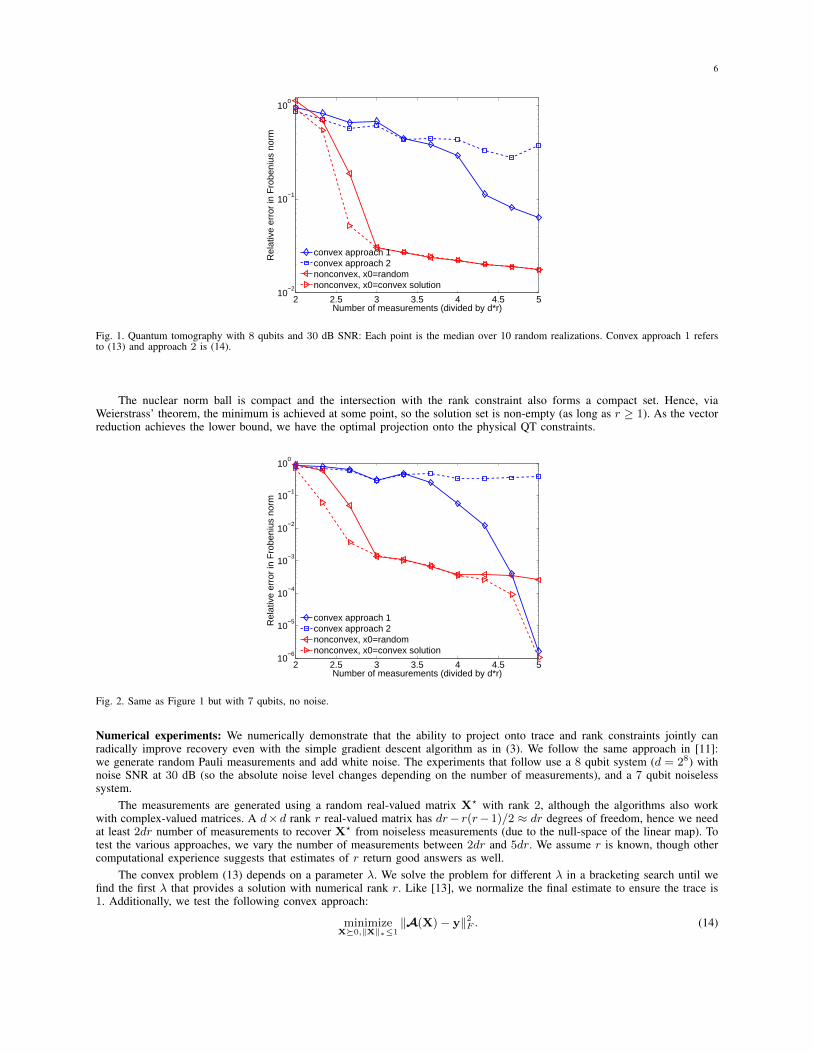
Fig. 1. Quantum tomography with 8 qubits and 30 dB SNR: Each point is the median over 10 random realizations. Convex approach 1 refersto (13) and approach 2 is (14).

The nuclear norm ball is compact and the intersection with the rank constraint also forms a compact set. Hence, viaWeierstrass’ theorem, the minimum is achieved at some point, so the solution set is non-empty (as long as r ≥ 1). As the vectorreduction achieves the lower bound, we have the optimal projection onto the physical QT constraints.

2 2.5 3 3.5 4 4.5 510

−6

10−5

10−4

10−3

10−2

10−1

100

Number of measurements (divided by d*r)

Rel

ativ

e er

ror

in F

robe

nius

nor

m

convex approach 1convex approach 2nonconvex, x0=randomnonconvex, x0=convex solution

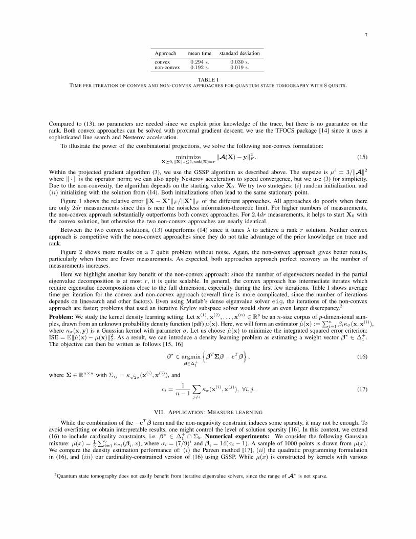
Fig. 2. Same as Figure 1 but with 7 qubits, no noise.

Numerical experiments: We numerically demonstrate that the ability to project onto trace and rank constraints jointly canradically improve recovery even with the simple gradient descent algorithm as in (3). We follow the same approach in [11]:we generate random Pauli measurements and add white noise. The experiments that follow use a 8 qubit system (d = 28) withnoise SNR at 30 dB (so the absolute noise level changes depending on the number of measurements), and a 7 qubit noiselesssystem.

The measurements are generated using a random real-valued matrix X? with rank 2, although the algorithms also workwith complex-valued matrices. A d×d rank r real-valued matrix has dr− r(r− 1)/2 ≈ dr degrees of freedom, hence we needat least 2dr number of measurements to recover X? from noiseless measurements (due to the null-space of the linear map). Totest the various approaches, we vary the number of measurements between 2dr and 5dr. We assume r is known, though othercomputational experience suggests that estimates of r return good answers as well.

The convex problem (13) depends on a parameter λ. We solve the problem for different λ in a bracketing search until wefind the first λ that provides a solution with numerical rank r. Like [13], we normalize the final estimate to ensure the trace is1. Additionally, we test the following convex approach:

minimizeX�0,‖X‖∗≤1

‖A(X)− y‖2F . (14)

7

Approach mean time standard deviation

convex 0.294 s. 0.030 s.non-convex 0.192 s. 0.019 s.

TABLE ITIME PER ITERATION OF CONVEX AND NON-CONVEX APPROACHES FOR QUANTUM STATE TOMOGRAPHY WITH 8 QUBITS.

Compared to (13), no parameters are needed since we exploit prior knowledge of the trace, but there is no guarantee on therank. Both convex approaches can be solved with proximal gradient descent; we use the TFOCS package [14] since it uses asophisticated line search and Nesterov acceleration.

To illustrate the power of the combinatorial projections, we solve the following non-convex formulation:

minimizeX�0,‖X‖∗≤1,rank(X)=r

‖A(X)− y‖2F . (15)

Within the projected gradient algorithm (3), we use the GSSP algorithm as described above. The stepsize is µi = 3/‖A‖2where ‖ · ‖ is the operator norm; we can also apply Nesterov acceleration to speed convergence, but we use (3) for simplicity.Due to the non-convexity, the algorithm depends on the starting value X0. We try two strategies: (i) random initialization, and(ii) initializing with the solution from (14). Both initializations often lead to the same stationary point.

Figure 1 shows the relative error ‖X −X?‖F /‖X?‖F of the different approaches. All approaches do poorly when thereare only 2dr measurements since this is near the noiseless information-theoretic limit. For higher numbers of measurements,the non-convex approach substantially outperforms both convex approaches. For 2.4dr measurements, it helps to start X0 withthe convex solution, but otherwise the two non-convex approaches are nearly identical.

Between the two convex solutions, (13) outperforms (14) since it tunes λ to achieve a rank r solution. Neither convexapproach is competitive with the non-convex approaches since they do not take advantage of the prior knowledge on trace andrank.

Figure 2 shows more results on a 7 qubit problem without noise. Again, the non-convex approach gives better results,particularly when there are fewer measurements. As expected, both approaches approach perfect recovery as the number ofmeasurements increases.

Here we highlight another key benefit of the non-convex approach: since the number of eigenvectors needed in the partialeigenvalue decomposition is at most r, it is quite scalable. In general, the convex approach has intermediate iterates whichrequire eigenvalue decompositions close to the full dimension, especially during the first few iterations. Table I shows averagetime per iteration for the convex and non-convex approach (overall time is more complicated, since the number of iterationsdepends on linesearch and other factors). Even using Matlab’s dense eigenvalue solver eig, the iterations of the non-convexapproach are faster; problems that used an iterative Krylov subspace solver would show an even larger discrepancy.2

Problem: We study the kernel density learning setting: Let x(1),x(2), . . . ,x(n) ∈ Rp be an n-size corpus of p-dimensional sam-ples, drawn from an unknown probability density function (pdf) µ(x). Here, we will form an estimator µ(x) :=

∑ni=1 βiκσ(x,x(i)),

where κσ(x,y) is a Gaussian kernel with parameter σ. Let us choose µ(x) to minimize the integrated squared error criterion:ISE = E‖µ(x) − µ(x)‖22. As a result, we can introduce a density learning problem as estimating a weight vector β? ∈ ∆+

1 .The objective can then be written as follows [15, 16]

β? ∈ argminβ∈∆+

1

{βTΣβ − cTβ

}, (16)

where Σ ∈ Rn×n with Σij = κ√2σ(x(i),x(j)), and

ci =1

n− 1

∑j 6=i

κσ(x(i),x(j)), ∀i, j. (17)

VII. APPLICATION: MEASURE LEARNING

While the combination of the −cTβ term and the non-negativity constraint induces some sparsity, it may not be enough. Toavoid overfitting or obtain interpretable results, one might control the level of solution sparsity [16]. In this context, we extend(16) to include cardinality constraints, i.e. β? ∈ ∆+

1 ∩ Σk. Numerical experiments: We consider the following Gaussianmixture: µ(x) = 1

5

∑5i=1 κσi(βi, x), where σi = (7/9)i and βi = 14(σi − 1). A sample of 1000 points is drawn from µ(x).

We compare the density estimation performance of: (i) the Parzen method [17], (ii) the quadratic programming formulationin (16), and (iii) our cardinality-constrained version of (16) using GSSP. While µ(x) is constructed by kernels with various

2Quantum state tomography does not easily benefit from iterative eigenvalue solvers, since the range of A∗ is not sparse.

8

−15 −10 −5 0 5 100

0.02

0.04

0.06

0.08

0.1

0.12

0.14

x

Pro

babi

lity

True pdfParzen windowQuad. Prog.True kernel mean position

0 200 400 600 800 10000

1

2

3x 10

−3

Wei

ghts

Quad. Prog.

0 200 400 600 8000

0.2

0.4

Sample point indices

Wei

ghts

s = 5

−15 −10 −5 0 5 100

0.02

0.04

0.06

0.08

0.1

0.12

0.14

x

Pro

babi

lity

True pdfEstimated pdf for s = 5True kernel meansEstimated kernel means

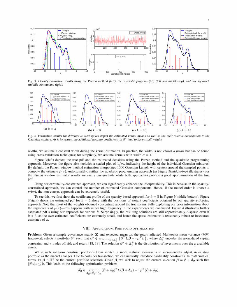
Fig. 3. Density estimation results using the Parzen method (left), the quadratic program (16) (left and middle-top), and our approach(middle-bottom and right).

−15 −10 −5 0 5 100

0.02

0.04

0.06

0.08

0.1

0.12

0.14

x

Pro

babi

lity

True pdfEstimated pdf for s = 3True kernel meansEstimated kernel means

(a) k = 3

−15 −10 −5 0 5 100

0.02

0.04

0.06

0.08

0.1

0.12

0.14

x

True pdfEstimated pdf for s = 8True kernel meansEstimated kernel means

(b) k = 8

−15 −10 −5 0 5 100

0.02

0.04

0.06

0.08

0.1

0.12

0.14

x

True pdfEstimated pdf for s = 10Estimated kernel meansTrue kernel means

(c) k = 10

−15 −10 −5 0 5 100

0.02

0.04

0.06

0.08

0.1

0.12

0.14

x

True pdfEstimated pdf for s = 15True kernel meansEstimated kernel means

(d) k = 15

Fig. 4. Estimation results for different k: Red spikes depict the estimated kernel means as well as the their relative contribution to theGaussian mixture. As k increases, the additional nonzero coefficients in β? tend to have small weights.

widths, we assume a constant width during the kernel estimation. In practice, the width is not known a priori but can be foundusing cross-validation techniques; for simplicity, we assume kernels with width σ = 1.

Figure 3(left) depicts the true pdf and the estimated densities using the Parzen method and the quadratic programmingapproach. Moreover, the figure also includes a scaled plot of 1/σi, indicating the height of the individual Gaussian mixtures.By default, the Parzen window method estimation interpolates 1000 Gaussian kernels with centers around the sampled points tocompute the estimate µ(x); unfortunately, neither the quadratic programming approach (as Figure 3(middle-top) illustrates) northe Parzen window estimator results are easily interpretable while both approaches provide a good approximation of the truepdf.

Using our cardinality-constrained approach, we can significantly enhance the interpretability. This is because in the sparsity-constrained approach, we can control the number of estimated Gaussian components. Hence, if the model order is known apriori, the non-convex approach can be extremely useful.

To see this, we first show the coefficient profile of the sparsity based approach for k = 5 in Figure 3(middle-bottom). Figure3(right) shows the estimated pdf for k = 5 along with the positions of weight coefficients obtained by our sparsity enforcingapproach. Note that most of the weights obtained concentrate around the true means, fully exploiting our prior information aboutthe ingredients of µ(x)—this happens with rather high frequency in the experiments we conducted. Figure 4 illustrates furtherestimated pdf’s using our approach for various k. Surprisingly, the resulting solutions are still approximately 5-sparse even ifk > 5, as the over-estimated coefficients are extremely small, and hence the sparse estimator is reasonably robust to inaccurateestimates of k.

VIII. APPLICATION: PORTFOLIO OPTIMIZATION

Problem: Given a sample covariance matrix Σ and expected mean µ, the return-adjusted Markowitz mean-variance (MV)framework selects a portfolio β? such that β? ∈ argmin

β∈∆+1

{βTΣβ − τµTβ

}, where ∆+

1 encodes the normalized capitalconstraint, and τ trades off risk and return [18, 19]. The solution β? ∈ ∆+

1 is the distribution of investments over the p availableassets.

While such solutions construct portfolios from scratch, a more realistic scenario is to incrementally adjust an existingportfolio as the market changes. Due to costs per transaction, we can naturally introduce cardinality constraints. In mathematicalterms, let β ∈ Rp be the current portfolio selection. Given β, we seek to adjust the current selection β = β + δβ such that‖δβ‖0 ≤ k. This leads to the following optimization problem:

δ∗β ∈ argminδβ∈Σk∩∆λ

(β + δβ)TΣ(β + δβ)− τµT (β + δβ),

9

280 300 320 340 360 380 40010

−5

10−4

10−3

10−2

10−1

100

m

Rel

ativ

e E

rror

Approach 1Approach 2

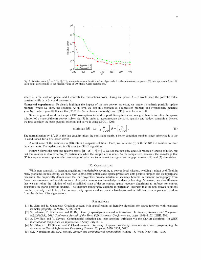
Fig. 5. Relative error ‖β−β?‖2/‖β?‖2 comparison as a function of m: Approach 1 is the non-convex approach (3), and approach 2 is (18).Each point corresponds to the median value of 30 Monte-Carlo realizations.

where λ is the level of update, and k controls the transactions costs. During an update, λ = 0 would keep the portfolio valueconstant while λ > 0 would increase it.Numerical experiments: To clearly highlight the impact of the non-convex projector, we create a synthetic portfolio updateproblem, where we know the solution. As in [19], we cast this problem as a regression problem and synthetically generatey = Xβ? where p = 1000 such that β? ∈ ∆λ (λ is chosen randomly), and ‖β?‖0 = k for k = 100.

Since in general we do not expect RIP assumptions to hold in portfolio optimization, our goal here is to refine the sparsesolution of a state-of-the-art convex solver via (3) in order to accommodate the strict sparsity and budget constraints. Hence,we first consider the basis pursuit criterion and solve it using SPGL1 [20]:

minimize ‖β‖1 s.t.[

X1T /√p

]β =

[y

λ/√p

]. (18)

The normalization by 1/√p in the last equality gives the constraint matrix a better condition number, since otherwise it is too

ill-conditioned for a first-order solver.Almost none of the solutions to (18) return a k-sparse solution. Hence, we initialize (3) with the SPGL1 solution to meet

the constraints. The update step in (3) uses the GSHP algorithm.

Figure 5 shows the resulting relative errors ‖β−β?‖2/‖β?‖2. We see that not only does (3) return a k-sparse solution, butthat this solution is also closer to β?, particularly when the sample size is small. As the sample size increases, the knowledge thatβ? is k-sparse makes up a smaller percentage of what we know about the signal, so the gap between (18) and (3) diminishes.

IX. CONCLUSIONS

While non-convexity in learning algorithms is undesirable according to conventional wisdom, avoiding it might be difficult inmany problems. In this setting, we show how to efficiently obtain exact sparse projections onto positive simplex and its hyperplaneextension. We empirically demonstrate that our projectors provide substantial accuracy benefits in quantum tomography fromfewer measurements and enable us to exploit prior non-convex knowledge in density learning. Moreover, we also illustratethat we can refine the solution of well-established state-of-the-art convex sparse recovery algorithms to enforce non-convexconstraints in sparse portfolio updates. The quantum tomography example in particular illustrates that the non-convex solutionscan be extremely useful; here, the non-convexity appears milder, since a fixed-rank matrix still has extra degrees of freedomfrom the choice of its eigenvectors.

REFERENCES

[1] R. Garg and R. Khandekar. Gradient descent with sparsification: an iterative algorithm for sparse recovery with restrictedisometry property. In ICML. ACM, 2009.

[2] S. Bahmani, P. Boufounos, and B. Raj. Greedy sparsity-constrained optimization. In Signals, Systems and Computers(ASILOMAR), 2011 Conference Record of the Forty Fifth Asilomar Conference on, pages 1148–1152. IEEE, 2011.

[3] A. Kyrillidis and V. Cevher. Combinatorial selection and least absolute shrinkage via the CLASH algorithm. In IEEEInternational Symposium on Information Theory, July 2012.

[4] M. Pilanci, L. El Ghaoui, and V. Chandrasekaran. Recovery of sparse probability measures via convex programming. InAdvances in Neural Information Processing Systems 25, pages 2429–2437, 2012.

[5] G.L. Nemhauser and L.A. Wolsey. Integer and combinatorial optimization, volume 18. Wiley New York, 1988.

10

[6] E. Candes, J. Romberg, and T. Tao. Robust uncertainty principles: Exact signal reconstruction from highly incompletefrequency information. IEEE Trans. on Information Theory, 52(2):489 – 509, February 2006.

[7] S. Foucart. Sparse recovery algorithms: sufficient conditions in terms of restricted isometry constants. Proceedings of the13th International Conference on Approximation Theory, 2010.

[8] A. Kyrillidis and V. Cevher. Recipes on hard thresholding methods. Dec. 2011.[9] Raghu Meka, Prateek Jain, and Inderjit S. Dhillon. Guaranteed rank minimization via singular value projection. In NIPS

Workshop on Discrete Optimization in Machine Learning, 2010.[10] Y.K. Liu. Universal low-rank matrix recovery from Pauli measurements. In NIPS, pages 1638–1646, 2011.[11] D. Gross, Y.-K. Liu, S. T. Flammia, S. Becker, and J. Eisert. Quantum state tomography via compressed sensing. Phys.

Rev. Lett., 105(15):150401, Oct 2010.[12] L. Mirsky. Symmetric gauge functions and unitarily invariant norms. The quarterly journal of mathematics, 11(1):50–59,

1960.[13] S.T. Flammia, D. Gross, Y.K. Liu, and J. Eisert. Quantum tomography via compressed sensing: error bounds, sample

complexity and efficient estimators. New Journal of Physics, 14(9):095022, 2012.[14] Stephen Becker, Emmanuel Candes, and Michael Grant. Templates for convex cone problems with applications to sparse

signal recovery. Mathematical Programming Computation, pages 1–54, 2011.[15] D. Kim. Least squares mixture decomposition estimation. PhD thesis, 1995.[16] F. Bunea, A.B. Tsybakov, M.H. Wegkamp, and A. Barbu. SPADES and mixture models. The Annals of Statistics,

38(4):2525–2558, 2010.[17] E. Parzen. On estimation of a probability density function and mode. The annals of mathematical statistics, 33(3):1065–

1076, 1962.[18] V. DeMiguel, L. Garlappi, F.J. Nogales, and R. Uppal. A generalized approach to portfolio optimization: Improving

performance by constraining portfolio norms. Management Science, 55(5):798–812, 2009.[19] J. Brodie, I. Daubechies, C. De Mol, D. Giannone, and I. Loris. Sparse and stable Markowitz portfolios. Proceedings of

the National Academy of Sciences, 106(30):12267–12272, 2009.[20] E. van den Berg and M. P. Friedlander. Probing the Pareto frontier for basis pursuit solutions. SIAM J. Sci. Comput.,

31(2):890–912, 2008.