context-bounded analysis for concurrent
TRANSCRIPT
Logical Methods in Computer ScienceVol. 7 (4:04) 2011, pp. 1–48www.lmcs-online.org
Submitted Jan. 31, 2010Published Nov. 23, 2011
CONTEXT-BOUNDED ANALYSIS FOR CONCURRENT PROGRAMS
WITH DYNAMIC CREATION OF THREADS
MOHAMED FAOUZI ATIG a, AHMED BOUAJJANI b, AND SHAZ QADEER c
a Uppsala University, Swedene-mail address: mohamed [email protected]
b LIAFA, University Paris Diderot, Francee-mail address: [email protected]
c Microsoft Research, Redmond, WA, USAe-mail address: [email protected]
Abstract. Context-bounded analysis has been shown to be both efficient and effectiveat finding bugs in concurrent programs. According to its original definition, context-bounded analysis explores all behaviors of a concurrent program up to some fixed numberof context switches between threads. This definition is inadequate for programs that createthreads dynamically because bounding the number of context switches in a computationalso bounds the number of threads involved in the computation. In this paper, we proposea more general definition of context-bounded analysis useful for programs with dynamicthread creation. The idea is to bound the number of context switches for each threadinstead of bounding the number of switches of all threads. We consider several variantsbased on this new definition, and we establish decidability and complexity results for theanalysis induced by them.
Introduction
The verification of multithreaded programs is a challenging problem both from the theoreti-cal and the practical point of view. (We consider here programs with parallel threads whichmay use local variables as well as shared (global) variables.) Assuming that the variablesof the program range over a finite domain (which can be obtained using some abstractionon the manipulated data), there are several aspects in multithreaded programs which maketheir analysis complex or even undecidable in general [Ram00].
Indeed, it is well known that for instance in the case where each thread can be modeledas a finite-state system, the state space of the program grows exponentially w.r.t. thenumber of threads, and the reachability problem is PSPACE-hard. Moreover, if threads aremodeled as pushdown systems, which corresponds to allowing unbounded depth (recursive)
1998 ACM Subject Classification: D.2.4, D.3.1, F.4.3, I.2.2.Key words and phrases: Pushdown Systems, Program Verification, Reachability Analysis.A shorter version of this paper has been published in the Proceedings of TACAS 2009, LNCS 5505.
LOGICAL METHODSl IN COMPUTER SCIENCE DOI:10.2168/LMCS-7 (4:04) 2011
c© M.F. Atig, A. Bouajjani, and S. QadeerCC© Creative Commons
2 M.F. ATIG, A. BOUAJJANI, AND S. QADEER
procedure calls in the program, then the reachability problem becomes undecidable as soonas two threads are considered.
Context-bounding has been proposed in [QR05] as a suitable technique for the analysisof multithreaded programs. The idea is to consider only the computations of the programthat perform at most some fixed number of context switches between threads. (At eachpoint only one thread is active and can modify the global variables, and a context-switchhappens when the active thread terminates or is interrupted, and a pending one is ac-tivated.) The state space which must be explored may still be unbounded in presence ofrecursive procedure calls, but the context-bounded reachability problem is decidable even inthis case. In fact, context-bounding provides a very useful tradeoff between computationalcomplexity and verification coverage. This tradeoff is based on three important properties.First, context-bounded verification can be performed more efficiently than unbounded veri-fication. From the complexity-theoretic point of view, it can be seen that context-boundedreachability is an NP-complete problem (even in the case of pushdown threads). Second,many concurrency errors, such as data races and atomicity violations, are manifested in ex-ecutions with few context switches [MQ07]. Finally, verifying all executions of a concurrentprogram up to a context bound provides an intuitive and meaningful notion of coverage tothe programmer.
While the concept of context-bounding is adequate for multithreaded programs witha (fixed) finite number of threads, the question we consider in this paper is whether thisconcept is still adequate when dynamic creation of threads is considered.
Dynamic thread creation is useful for modeling several important aspects, e.g., (1)unbounded number of concurrent executions of software modules such as file systems, devicedrivers, non-blocking data structures etc., or (2) creation of asynchronous activity such asforking a thread, queuing a closure to a threadpool with or without timers, callbacks, etc.Both these sources are very important for modeling operating system components; they arelikely to become important even for application software as it becomes increasingly parallelin order to harness the power of multi-core architectures.
We argue that the “classical” notion of context-bounding which has been used so farin the existing work is actually too restrictive in this case. Indeed, bounding the numberof context switches in a computation also bounds the number of threads involved. In thispaper, we propose a more general definition of context-bounded analysis useful for programswith dynamic thread creation. The idea is to bound the number of context switches foreach thread instead of bounding the number of switches of all threads. We consider severalvariants based on this new definition, and we establish decidability and complexity resultsfor the analysis induced by them.
We introduce a notion of K-bounded computations where each of the involved threadscan be interrupted and resumed at most K times. In fact, we consider that when a threadis created, the number of context switches it can perform is the one of its ancestor (at themoment of the creation) minus 1. Notice that the number of context switches by all threadsin a computation is not bounded since the number of threads involved is not bounded.
In the case of finite-state threads, we prove that this problem is as hard as the coverabil-ity problem for vector addition systems with states (or, Petri nets) (which is EXPSPACE-complete). The reduction from our problem to the coverability problem of vector additionsystems with states is based on the simple idea of counting the number of pending threadsfor different values of the global and local states, as well as of the number of switches that
3
these threads are allowed to perform. Conversely, we prove that the coverability prob-lem of vector addition systems with states can be reduced to the 2-bounded reachabilityproblem. These results show that in the case of dynamic thread creation, considering thenotion of context-bounding for each individual thread makes the complexity jumps from NP-completeness to EXPSPACE-completeness, even in the case of finite-state threads. Then,an interesting question is whether it is possible to have a notion of context-bounding witha lower complexity. We propose for that the notion of stratified context-bounding. Theidea is to consider computations where the scheduling of the threads is ordered accordingto their number of allowed switches: First, threads of level K (the level means here thenumber of allowed switches) are scheduled generating threads of level K − 1, then threadsof level K − 1 are scheduled, and so on. Again, notice that K-stratified computationsmay have an unbounded number of context switches since it is possible to schedule anunbounded number of threads at each level. This concept generalizes obviously the “clas-sical” notion of context-bounding. We prove that, for finite-state threads, the K-stratifiedcontext-bounded reachability problem is NP-complete (i.e., it matches the complexity ofthe “classical” context-bounded reachability problem). The proof is by a reduction to thesatisfiability problem of existential Presburger formulas.
Then, we consider the case of dynamic creation of pushdown threads. We prove that,surprisingly, the K-bounded reachability problem is in fact decidable, and that the sameholds also for the K-stratified context-bounded reachability problem. To establish theseresults, we prove that these problems (for pushdown threads) can be reduced to theircorresponding problems for finite-state threads. This reduction is not trivial. The mainideas behind the reduction are as follows: First, the K-bounded behaviors of each singlethread can be represented by a labeled pushdown system which (1) makes visible (as labels)on its transitions the created threads, and (2) guesses points of interruption-resumption andthe corresponding values of the global states. (These guesses are also made visible on thetransitions.) Then, the main problem is to “synchronize” these labeled pushdown systemsso that their guesses can be validated. The key observation is that it is possible to abstractthese systems without loss of preciseness by finite-state systems. This is due to the fact thatwe can consider that some of the generated threads can be lost (since they can be seen asthreads that are never activated), and therefore we can reason about the downward closureof the languages of the labeled pushdown systems mentioned above (w.r.t. suitable sub-wordrelation). This downward closure is in fact always regular and effectively constructible.
Related work. In the last few years, several implementations and algorithmic improve-ments have been proposed for context-bounded verification [BESS05, MQ07, SES08, LTKR08,LR08, LMP09]. For instance, context-bounded verification has been implemented in explicit-state model checkers such as CHESS [MQ07] and SPIN [ZJ08]; it has also been implementedin symbolic model checkers such as SLAM [QW04], jMoped [SES08], and in [LR08]. In thispaper, we propose more general definitions of context-bounded analysis useful for programswith dynamic thread creation.
Several models based on rewriting systems or networks of pushdown systems havebeen considered to model multithreaded programs [LS98, EP00, SS00, Mo02, BT03, BT05].While these models allow to model dynamic thread creation, they only allow communicationbetween processes in a very restrictive way.
4 M.F. ATIG, A. BOUAJJANI, AND S. QADEER
In [BMOT05], a model based on networks of pushdown systems called CDPN wasproposed. While this model allows dynamic creation of processes, it allows only a restrictedform of synchronization where a process has the right to read only the control states of itsimmediate children (i.e., the processes it has created).
A symbolic algorithm for over-approximating reachability in Boolean programs withunboundedly many threads was given in [CKS06, CKS07]. Our approach complementsthese techniques since they are able to prove that a safety property of interest holds. Whileour work is useful for effectively detecting bad behaviors of the analyzed programs.
A recent paper proposes an algorithm for the verification problem for parametrizedconcurrent programs with procedural calls under a k-round-robin schedule [LMP10]. Ourwork is more powerful than this framework as long as the data domain is bounded.
1. Preliminary definitions and notations
In this section, we introduce some basic definitions and notations that will be used in therest of the paper.
1.1. Integers, functions, and vectors.
Integers. Let Z be the set of integers and N be the set of positive integers (or naturalnumbers). For every i, j ∈ Z such that i ≤ j, we use [i, j] and [i, j[ to denote respectivelythe sets {k ∈ Z | i ≤ k ≤ j} and {k ∈ Z | i ≤ k < j}.
Functions. Let A and B be two sets. We denote by [A→ B] the set of all functions from Ato B. If f, g are two functions from A to N, then we write g ≤ f if and only if g(a) ≤ f(a)for all a ∈ A. We use f + g (resp. f − g if g ≤ f) to denote the function from A to N
defined as follows: (f + g)(a) = f(a) + g(a) (resp. (f − g)(a) = f(a)− g(a)) for all a ∈ A.
For every subset C ⊆ A, we use IdCA to denote the function from A to N defined as follows:
IdCA(a) =
{
1 if a ∈ C0 if a ∈ (A \ C)
(1.1)
In particular, Id∅A denotes the function that maps any element of A to 0.
Vectors. Let n be a natural number and A be a set. An n-dim vector v over A is an elementof An. For every i ∈ [1, n], we denote by v[i] ∈ A the ith component of v. Given j ∈ [1, n]and a ∈ A, we denote by v[j ← a] the n-dim vector v′ over A such that v′[j] = a andv′[k] = v[k] for all k ∈ [1, n] and k 6= j.
Vectors of integers. The order relation ≤ between integers is generalized in a pointwisemanner to vectors of integers. We write 0n to denote the n-dim vector v over Z such thatv[i] = 0 for all i ∈ [1, n]. We trivially extend the addition and subtraction operations overintegers to vectors of integers.
5
1.2. Words and languages. Given a finite set Σ called an alphabet and whose elementsare called letters or symbols, a word u over Σ is either a finite sequence of letters in Σ orthe empty word ǫ. The length of u is denoted by |u|. (We assume that |ǫ| = 0.) For everya ∈ Σ, we use |u|a to denote the number of occurrences of a in u. For every j ∈ [1, |u|], weuse u(j) to denote the jth letter of u.
A language L over Σ is a (possibly infinite) set of words over Σ. We adopt the widespreadnotations Σ∗ and Σ+ to represent respectively the languages containing all words and allnon-empty words over Σ. We use also Σǫ to denote the set Σ ∪ {ǫ}.
We denote by �⊆ Σ∗×Σ∗ the subword relation defined as follows: For every u, v ∈ Σ∗,u � v if and only if: (1) u = ǫ, or (2) there are i1, i2 . . . , i|u| ∈ [1, |v|] such that i1 < i2 <· · · < i|u| and u(j) = v(ij) for all j ∈ [1, |u|]. Given a language L ⊆ Σ∗, the downwardclosure of L is the language L ↓= {u ∈ Σ∗ | ∃v ∈ L, u � v}.
Let Θ be a subset of Σ. Given a word u ∈ Σ∗, we denote by u|Θ the projection of u overΘ, i.e., the word obtained from u by erasing all the symbols that are not in Θ. This definitionis extended to languages as follows: If L is a language over Σ, then L|Θ = {u|Θ | u ∈ L}.
The Parikh image of a word u ∈ Σ∗ is a function from Σ to N such that: For everya ∈ Σ, Parikh(u)(a) = |u|a. Accordingly, the Parikh image of a language L ⊆ Σ∗, writtenParikh(L), is the set of Parikh images of u ∈ L.
Let Σ1 and Σ2 be two alphabets. A homomorphism h is a function from Σ∗1 to Σ∗
2 suchthat h(ǫ) = ǫ and h(uv) = h(u)h(v) for all u, v ∈ Σ∗
1. By definition, the homomorphism h iscompletely characterized by the function fh : Σ1 → Σ∗
2 s.t. for any a ∈ Σ1, fh(a) = h(a).
1.3. Transition systems. A transition system is a triplet T = (C,Σ,→) where: (1) C isa (possibly infinite) set of configurations (also called states), (2) Σ is a finite set of labels(or actions), and (3) →⊆ C × Σǫ × C is a transition relation.
Given two configurations c, c′ ∈ C and an action a ∈ Σ, we write c a−→T c′ if (c, a, c′) ∈→.A finite run ρ of T from c to c′ is a finite sequence c0a1c1a2 · · · ancn, for some n ≥ 1, such
that: (1) c0 = c and cn = c′, and (2) ciai+1−−−→T ci+1 for all i ∈ [0, n[. In this case, we say
that ρ has length n and is labelled by the word a1a2 · · · an.Let u ∈ Σ∗ be an input word. We write c
u==⇒n
T c′ if one of the following two cases holds:
(1) n = 0, c = c′, and u = ǫ, and (2) there is a run ρ of length n from c to c′ labelled
by u. We also write cu
==⇒∗T c′ to denote that c
u==⇒n
T c′ for some n ≥ 0. Finally, for every
C1, C2 ⊆ C, we have TracesT (C1, C2) = {u ∈ Σ∗ | ∃(c1, c2) ∈ C1 × C2 , c1u
==⇒∗T c2}.
1.4. Finite state automata. A finite state automaton (FSA for short) is a quintupleA = (Q,Σ,∆, I, F ) where: (1) Q is the finite non-empty set of states, (2) Σ is the finite setof input symbols (called also the input alphabet), (3) ∆ ⊆ (Q × Σǫ × Q) is the transitionrelation, (4) I ⊆ Q is the set of initial states, and (5) F ⊆ Q is the set of final states. Weuse q a−→A q′ to denote that (q, a, q′) is in ∆ .
The size of A, denoted by |A|, is defined by (|Q|+ |Σ|). We denote by T (A) = (Q,Σ,∆)the transition system associated toA. The language accepted (or recognized) byA is definedas follows L(A) = TracesT (A)(I, F ).
It is well known that the class of languages accepted by finite state automata (the classof rational (or regular) languages) is effectively closed under union, intersection, homomor-phism, and projection operations [HU79].
6 M.F. ATIG, A. BOUAJJANI, AND S. QADEER
1.5. Pushdown automata. A pushdown automaton (PDA for short) is a 7-tuple P =(P,Σ,Γ,∆, p0, γ0, F ) where:
• P is the finite non-empty set of states,• Σ is the finite set of input symbols (called also the input alphabet),• Γ is the finite set of stack symbols (called also the stack alphabet),• ∆ ⊆
(
(P × Γ)× Σǫ × (P × Γ≤2))
is the transition relation (where Γ≤2 = Γǫ ∪ Γ2).• p0 ∈ P is the initial state,• γ0 ∈ Γ is the initial stack symbol, and• F ⊆ P is the set of final states.
The size of P, denoted by |P|, is defined as (|P | + |Σ|+ |Γ|). We use 〈p, γ〉 a−→P〈p′, u〉
to denote that ((p, γ), a, (p′, u)) is in ∆.A configuration of P is a pair (p,w) where p ∈ P and w ∈ Γ∗. The set of all config-
urations of P is denoted by Conf (P). The transition system associated to P, denoted byT (P), is given by the tuple (Conf (P),Σ,→) where → is the smallest transition relationsuch that: if 〈p, γ〉 a−→P〈p
′, u〉, then (p, γw) a−→T (P) (p′, uw) for all w ∈ Γ∗. The language of
P is defined as follows L(P) = TracesT (P)({(p0, γ0)}, F × Γ∗).It is well known that the class of context-free languages (i.e., accepted by pushdown
automata) are closed under concatenation, union, Kleene star, homomorphism, projection,and intersection with a rational language. However, context-free languages are not closedunder complement and intersection [HU79].
Let us recall now that the downward closure of a context-free language, with respectto the subword relation, is effectively a rational language.
Theorem 1.1 ([Cou91]). If P is a PDA, then, it is possible to construct, in time and spaceexponential in |P|, a finite state automaton A such that L(A) = L(P) ↓ and the size of |A|is exponential in |P| in the worst case.
We can prove that the exponential blow-up in Theorem 1.1 can not be avoided. Thisis due to the fact that pushdown automata are more succinct than finite state automata.To show that, let us consider the following pushdown automaton P = ({p0, p1, p2}, {a},{⊥, γ0, . . . , γn},∆, p0,⊥, {p2}) where n ∈ N and ∆ is the transition relation composed fromthe following transitions:
(1) 〈p0,⊥〉ǫ−→P〈p1, γ0⊥〉,
(2) for every i ∈ [0, n[, 〈p1, γi〉ǫ−→〈p1, γi+1γi+1〉,
(3) 〈p1, γn〉a−→P〈p1, ǫ〉, and
(4) 〈p1,⊥〉ǫ−→P〈p2, ǫ〉.
It is easy to observe that L(P) = {a2n
} and therefore the minimal finite state automatonA recognizing L(P) ↓ has at least 2n states whereas the size of P is (n+ 5).
2. Dynamic network of concurrent pushdown systems
In this section, we introduce dynamic network of concurrent pushdown systems. Intuitively,a dynamic network of concurrent pushdown systems M models dynamic multithreadedprograms with (potentially) recursive procedure calls. Threads are modeled as pushdownprocesses which may spawn new threads (or processes). Each thread may have its localvariables and has also access to global variables. The values of local variables are modeledusing the stack alphabet Γ, whereas the values of the global variables are modeled using a
7
finite non-empty set of states Q. Transitions of the form 〈q, γ〉−→M〈q′, u〉 ⊲ ǫ correspond to
standard transitions of pushdown systems (popping γ and then pushing u while changingthe state from q to q′). Transitions of the form 〈q, γ〉−→M〈q
′, u〉 ⊲ γ′ correspond to standardtransitions of pushdown systems with a creation of a thread whose initial stack content isγ′ ∈ Γ. Transitions of the form 〈q, γ〉 7→M 〈q
′, u〉 correspond to interrupt the execution ofthe active thread after the performing the standard pushdown operations, and transitionsof the form q 7→M q′ ⊳ γ correspond to start/resume the execution of a pending threadwith topmost stack symbol γ′ ∈ Γ after changing the state from q to q′.
2.1. Syntax.
Definition 2.1 (DCPS). A dynamic network of concurrent pushdown system (DCPS forshort) is a tupleM = (Q,Γ,∆, q0, γ0) where:
• Q is the finite non-empty set of states,• Γ is a finite set of stack symbols (called also stack alphabet),• ∆ = ∆cr ∪∆in ∪∆rs where:− ∆cr ⊆
(
(Q× Γ)× (Q× Γ≤2)× Γǫ
)
is a finite set of (creation ) transitions.
− ∆in ⊆(
(Q× Γ)× (Q× Γ≤2))
is a finite set of (interruption) transitions.
− ∆rs ⊆(
Q× Γ×Q)
is a finite set of (resumption) transitions.• q0 is the initial state, and• γ0 is the initial stack symbol.
In the rest of the paper, we adopt the following notations: (1) 〈q, γ〉−→M〈q′, u〉 ⊲ α to
denote that(
(q, γ), (q′, u), α)
∈ ∆cr, (2) 〈q, γ〉 7→M 〈q′, u〉 to denote that
(
(q, γ), (q′, u))
∈
∆in, and (3) q 7→M q′ ⊳ γ to denote that(
q, γ, q′)
∈ ∆rs. The size of M is given by|M| = |Q|+ |Γ|.
When unbounded recursion is not considered, threads can be modeled as finite stateprocesses instead of pushdown systems. This corresponds to the special case where, for all((q, γ), (q′, u), α) ∈ ∆cr and ((q, γ), (q′, u)) ∈ ∆in, the pushed word u is of length at most 1.
Definition 2.2 (DCFS). A dynamic concurrent finite-state systems (DCFS for short) is aDCPS M = (Q,Γ,∆, q0, γ0) where, for all ((q, γ), (q′, u), α) ∈ ∆ and ((q, γ), (q′, u)) ∈ ∆,we have |u| ≤ 1.
2.2. Semantics.
Definition 2.3 (Local configurations of a DCPS). Let M = (Q,Γ,∆, q0, γ0) be a DCPS.A local configuration of a thread of M is a pair (w, i) where w ∈ Γ∗ is its call stack andi ∈ N is its switch number. Let Loc(M) denote the set of local configurations ofM.
Intuitively, the switch number of a thread is the number of interruptions/resumptionstogether with the switch number of its creator (at the moment of the creation) plus one.
Definition 2.4 (Configurations of a DCPS). Let M = (Q,Γ,∆, q0, γ0) be a DCPS. Aconfiguration c of a M is an element of Q × (Loc(M) ∪ {⊥}) × [Loc(M) → N]. We useConf (M) to denote the set of all configurations ofM.
8 M.F. ATIG, A. BOUAJJANI, AND S. QADEER
A configuration of the form (q, (w, i),Val ) (resp. (q,⊥,Val)) of M means that: (1)q ∈ Q is the value of the global store, (2) (w, i) is the local configuration of the active thread(resp. there is no active thread), and (3) Val : Loc(M) → N is a function that associatesfor each (w′, i′) ∈ Loc(M), the number of pending threads with local configuration (w′, i′).
Given a configuration c = (q, η,Val ) ∈ Conf (M), let State(c) = q, Active(c) = η, and
Idle(c) = Val . We use cinitM = (q0,⊥, Id{(γ0,0)}Loc(M)) to denote the initial configuration ofM.
Definition 2.5 (Transition system of a DCPS). LetM = (Q,Γ,∆, q0, γ0) be a DCPS. Thetransition system associated withM is given by T (M) = (Conf (M),Σ,→) where Σ = ∆and → is the smallest relation such that:
• if t = 〈q, γ〉−→M〈q′, u〉 ⊲ α, then (q, (γw, i),Val ) t−→T (M)(q
′, (uw, i),Val ′) for all w ∈ Γ∗,
i ∈ N, and Val ,Val ′ ∈ [Loc(M)→ N] such that:
− If α ∈ Γ, then Val ′ = Val + Id{(α,i+1)}Loc(M) .
− If α = ǫ, then Val ′ = Val .
• if t = 〈q, γ〉 7→M 〈q′, u〉, then (q, (γw, i),Val ) t−→T (M)(q′,⊥,Val + Id
{(uw,i+1)}Loc(M) ) for all
w ∈ Γ∗, i ∈ N, and Val ∈ [Loc(M)→ N].
• if t = q 7→M q′ ⊳ γ, then (q,⊥,Val + Id{(γw,i)}Loc(M) )
t−→T (M)(q′, (γw, i),Val ) for all w ∈ Γ∗,
i ∈ N, and Val ∈ [Loc(M)→ N].
where for every sets A and C such that C ⊆ A, IdCA denotes the function from A to N such
that IdCA = 1 if a ∈ C and IdCA(a) = 0 if a ∈ (A \ C) (see Equation. 1.1).
The transition (q, (γw, i),Val ) t−→T (M)(q′, (uw, i),Val ′), with t = 〈q, γ〉−→M〈q
′, u〉 ⊲ α,corresponds to the execution of pushdown operation (pop or push) with the possibility of acreation of a new thread (if α ∈ Γ) which is added to the set of pending threads. The created
thread gets the switch number i + 1. The transition (q, (γw, i),Val ) t−→T (M)(q′,⊥,Val ′),
with t = 〈q, γ〉 7→M 〈q′, u〉, corresponds to interrupt the execution of the current activethread after performing the pushdown operation: The local configuration (uw, i) of theactive thread is added to the set of the idle threads after incrementing its switch number.
The transition (q,⊥,Val) t−→T (M)(q′, (γw, i),Val ′), with t = q 7→M q′ ⊳ γ, corresponds to
start/resume (from the state q′) the execution of a pending thread with local configuration(γw, i).
2.3. Bounded semantics. Let M = (Q,Γ,∆, q0, γ0) be a DCPS. For every I ⊆ N, letConf I(M) denote the set of configurations of M such that c ∈ Conf I(M) if and only ifActive(c) ∈ Γ∗ × I. In the following, we restrict the behavior of T (M) to the set of runswhere the switch numbers of the active threads are always in I.
Definition 2.6 (Bounded transition system of a DCPS). For every I ⊆ N, TI(M) denotes
the transition system (Conf (M),∆,→I) where: For every c, c′ ∈ Conf (M), c t−→TI(M) c′ if
and only if: (1) c t−→T (M) c′, and (2) c ∈ Conf I(M) or c′ ∈ Conf I(M).
9
2.4. Reachability problems. Let M = (Q,Γ,∆, q0, γ0) be a DCPS. We consider thefollowing three notions of reachability:
Definition 2.7 (The state reachability problem). A state q ∈ Q is reachable byM if and
only if there are c ∈ Conf (M) and τ ∈ ∆∗ such that cinitMτ
==⇒∗T (M) c, Active(c) = ⊥, and
State(c) = q. The state reachability (SR for short) problem forM consists in deciding, fora given set F ⊆ Q, whether there is a state q ∈ F such that q is reachable byM.
Notice that we consider, in the definition of the state reachability problem, that the setof reachable configurations that we are interested in are those with no active thread. Thisis only for the sake of simplicity and does not constitute at all a restriction. Indeed, wecan show that the problem of checking whether there are c ∈ Conf (M) and τ ∈ ∆∗ such
that cinitMτ
==⇒∗T (M) c and State(c) ∈ F can be reduced to the state reachability problem for a
DCPSM′ = (Q,Γ,∆′, q0, γ0) built up fromM by adding to ∆ some transition rules thatinterrupt the execution of the active thread when the current state is in F .
Definition 2.8 (The k-bounded state reachability problem). Let k ∈ N. A state q ∈ Qis k-bounded reachable by M if and only if there are c ∈ Conf (M) and τ ∈ ∆∗ such
that cinitMτ
==⇒∗T[0,k](M) c, Active(c) = ⊥, and State(c) = q. The k-bounded state reachability
(BSR[k] for short) problem forM consists in deciding, for a given set F ⊆ Q, whether thereis a state q ∈ F such that q is k-bounded reachable byM.
Observe that, in BSR[k] problem, a bound k+1 is imposed on the number of switches(interruptions/resumptions) performed by each thread (together with the switch number ofits ancestor (at the moment of its creation) plus one). However, due to dynamic creationof threads, bounding the number of switches of each thread does not bound the numberof switches in the whole computation of the system (since an arbitrary large number ofthreads can be involved in these computations).
Definition 2.9 (The k-stratified state reachability problem). Let k ∈ N. A state q ∈ Q isk-stratified reachable by M if and only if there are τ0, τ1, . . . , τk ∈ ∆∗, and c1, . . . , ck+1 ∈Conf (M) such that State(ck+1) = q, Active(ck+1) = ⊥, and we have:
cinitMτ0==⇒∗
T{0}(M) c1τ1==⇒∗
T{1}(M) · · ·τk−1===⇒∗
T{k−1}(M) ckτk==⇒∗
T{k}(M) ck+1
The k-stratified state reachability (SSR[k] for short) problem for M consists in deciding,for a given F ⊆ Q, whether there is a state q ∈ F s.t. q is k-stratified reachable byM.
In the SSR[k] problem, a special kind of k-bounded computations (called stratifiedcomputations) are considered: In such a computation, threads are scheduled according totheir increasing switch number (from 0 to k): First, threads with switch number 0 arescheduled generating threads with switch number 1, then threads with switch number 1 arescheduled generating threads with switch number 2, and so on.
Observe that even in the case of stratified computations, an arbitrarily large number ofcontext switches may occur along a computation due to dynamic creation of threads. Veryparticular stratified computations are those where the whole number of context switches isbounded [QR05].
10 M.F. ATIG, A. BOUAJJANI, AND S. QADEER
3. The SR problem and the BSR[k] problem for DCFSs
In the following, we show that the SR problem and the BSR[k] problem for dynamic net-works of concurrent finite-state systems are as hard as the coverability problem for vectoraddition systems with states (which is EXPSPACE-complete).
Theorem 3.1. The SR problem and the BSR[k] problem, with k ≥ 2, for DCFSs areEXPSPACE-complete.
Next, we recall some basic definitions and notations about vector addition systemswith states (or equivalently, Petri nets). Then, this proof of Theorem 3.1 is structured asfollows: First, we show that the BSR[k] problem for DCFSs is polynomially reducible tothe SR problem for DCFSs (Proposition 3.4). Then, we show that the SR problem forDCFSs is polynomially reducible to the coverability problem for VASSs (Proposition 3.6).Finally, we prove that the coverability problem for VASSs is polynomially reducible to theBSR[2] problem for DCFSs (Proposition 3.8). As an immediate consequence of these resultsand Theorem 3.2, we obtain that the SR problem and the BSR[k] problem for DCFSs areEXPSPACE-complete.
3.1. Vector addition systems with states. A vector addition system with states (VASSfor short) is a tuple V = (n,Q,Σ, δ, q0,u0) where:
• n ∈ N is the dimension,• Q is the finite non-empty set of states,• Σ is the finite set of actions (or labels),• δ : Q× Σ→ Q× ([−1, 1])n is the displacement function,• q0 ∈ Q is the initial state, and• u0 is the initial n-dim vector over N such that 0 ≤ u0(i) ≤ 1 for all i ∈ [1, n].
The size of V, denoted by |V |, is defined as (n + |Q| + |Σ|). A configuration of V is apair (q,u) where q ∈ Q and u ∈ N
n. Given a configuration c = (q,u), we let State(c) = qand Val(c) = u. The set of all configurations of V is denoted by Conf (V).
The transition system associated to V, denoted by T (V), is given by (Conf (V),Σ,→),where → is the smallest transition relation satisfying the following condition: For everyq1, q2 ∈ Q and u1,u2 ∈ N
n, (q1,u1)a−→T (V)(q2,u2) if and only if δ((q1, a)) = (q2,u2 − u1).
A state q ∈ Q is reachable by V if and only if there are w ∈ Σ∗ and c ∈ Conf (V)
such that (q0,u0)w
==⇒∗T (V) c and State(c) = q. The coverability problem for V consists in
deciding, for a given set F ⊆ Q, whether there is q ∈ F such that q is reachable by V.
Theorem 3.2 ([Lip76, Rac78]). The coverability problem for vector addition systems withstates is EXPSPACE-complete.
3.2. From the BSR[k] problem for DCFSs to the SR problem for DCFSs. In thefollowing, we show that, for every k ∈ N, the BSR[k] for DCFSs is polynomially reducible tothe SR problem for DCFSs. Intuitively, given a DCFSM = (Q,Γ,∆, q0, γ0) and a naturalnumber k, we construct a DCFS M′ that records for each thread its switch number andcan execute only threads with recorded switch number less than k. Formally, the DCFSM′ = (Q′,Γ′,∆′, q′0, γ
′0) is defined as follows:
• Q′ = Q is a finite set of states,
11
• Γ′ = Γǫ × [0, k + 1] is a finite set of stack symbols. A stack symbol (α, i) corresponds toa thread with stack content α and switch number i.• ∆′ is the smallest transition relation satisfying the following conditions:− For every i ∈ [0, k] and 〈q, γ〉−→M〈q
′, u〉 ⊲ ǫ, then 〈q, (γ, i)〉−→M′〈q′, (u, i)〉 ⊲ ǫ.− For every i ∈ [0, k] and 〈q, γ〉−→M〈q
′, u〉 ⊲ α for some stack symbol α ∈ Γ, then〈q, (γ, i)〉−→M′〈q′, (u, i)〉 ⊲ (α, i + 1).
− For every i ∈ [0, k] and 〈q, γ〉 7→M 〈q′, u〉, then 〈q, (γ, i)〉 7→M′ 〈q′, (u, i + 1)〉.− For every i ∈ [0, k] and q 7→M q′ ⊳ γ, then q 7→M′ q′ ⊳ (γ, i).• q′0 = q0 is the initial state, and• γ′0 = (γ0, 0) is the initial stack symbol.
Observe that the size of the DCFSM′ is polynomial in the size of M. Moreover, therelation betweenM andM′ is given by the following lemma:
Lemma 3.3. Let q ∈ Q. q is k-bounded reachable byM iff q is reachable by M′.
The proof of Lemma 3.3 is done by induction on the length of the runs and is given inAppendix A.
As an immediate consequence of Lemma 3.3, we obtain the following result:
Proposition 3.4. Let k ≥ 1. The BSR[k] problem for DCFSs is polynomially reducible tothe SR problem for DCFSs.
3.3. From the SR problem for DCFSs to the coverability problem for VASSs.
In the following, we show that the SR problem for DCFSs is polynomially reducible tothe coverability problem for VASSs. For a given DCFS M = (Q,Γ,∆, q0, γ0), with Γ ={γ0, . . . , γn}, we can construct a VASS V = (m,P,Σ, δ, p0,u0) which has the followingstructure:
• m = n + 2 is the dimension of V. It is easy to observe that the dimension of V is equalto |Γǫ| which is the number of all possible stack contents of threads ofM.• P = (Q × (Γǫ ∪ {⊥})) ∪ {phalt} is the set of states of V (with phalt /∈ Q). A state of theform (q, w) ∈ Q×Γǫ (resp. (q,⊥)) of V means that the state ofM is q and that the stackcontent of the active thread is w (resp. there is no active thread). The state phalt is usedin order to interrupt the simulation ofM by V.• Σ = ∆ is the input alphabet of V.• δ : P × Σ → P × ([−1, 1])m is the transition function of V defined as follows: For everyp ∈ P and t ∈ Σ, we have:− δ(p, t) = (p′,0m) if there are q, q′ ∈ Q, γ ∈ Γ, and u ∈ Γǫ such that t = 〈q, γ〉−→M
〈q′, u〉 ⊲ ǫ, p = (q, γ), and p′ = (q′, u). This corresponds to the simulation of atransition rule ofM without thread creation.
− δ(p, t) = (p′,0m[i ← 1]) if i ∈ [1,m[ and there are q, q′ ∈ Q, γ ∈ Γ, and u ∈ Γǫ suchthat t = 〈q, γ〉−→M 〈q
′, u〉 ⊲ γi−1, p = (q, γ), and p′ = (q′, u). This corresponds to thesimulation of a transition rule ofM with thread creation.
− δ(p, t) = (p′,0m[j ← 1]) if j ∈ [1,m], and there are q, q′ ∈ Q, γ ∈ Γ, and u ∈ Γǫ suchthat t = 〈q, γ〉 7→M 〈q′, u〉, p = (q, γ), p′ = (q′,⊥), u = ǫ if j = m, and u = γj−1
if j < m. This corresponds to the interruption of the execution of the current activethread.
12 M.F. ATIG, A. BOUAJJANI, AND S. QADEER
− δ(p, t) = (p′,0m[i ← −1]) if i ∈ [1,m[, and there are q, q′ ∈ Q, such that t = q 7→M
q′ ⊳ γi−1, p = (q,⊥), and p′ = (q′, γi−1). This corresponds to the execution of apending thread with topmost stack symbol γi−1.
− δ(p, t) = (phalt,0m) otherwise. This indicates the end of the simulation of M by V
whenever the transition t can not be applied from the state p.• u0 = (1, 0, . . . , 0). This corresponds to the initial pending thread ofM (i.e., initially Mhas one pending thread with local configuration (γ0, 0)).• p0 = (q0,⊥) is the initial state of V. This corresponds to the initial state q0 ofM.
Observe that the size of V is polynomial in the size of M. Moreover, the relationbetweenM and V is given by the following lemma:
Lemma 3.5. Let q ∈ Q. q is reachable byM if and only if (q,⊥) is reachable by V.
The proof of Lemma 3.5 is done by induction on the length of the runs and is given inAppendix B.
As an immediate consequence of Lemma 3.5, we obtain the following result:
Proposition 3.6. The SR problem for DCFSs is polynomially reducible to the coverabilityproblem for VASSs.
3.4. From the coverability problem for VASSs to the BSR[2] problem for DCFSs.
In the following, we prove that the coverability problem for VASSs is polynomially reducibleto the BSR[2] for DCFSs. Given a VASS V = (n,Q,Σ, δ, q0,u0), we construct a DCFSMsuch that the coverability problem for V is reducible to the BSR[2] problem for M. Weassume w.l.o.g that for every q ∈ Q and a ∈ Σ, δ(q, a) ∈ Q×{u ∈ N
n |∑n
i=1 abs(u[i]) ≤ 1}and u0 = 0n. Intuitively, M has, for each i ∈ [1, n], a stack symbol γi such that thenumber of pending threads with local configuration (γi, 2) denotes the current value of thei-th counter of V. The systemM has also a special stack symbol γ′0 such that the pendingthreads with local configuration (γ′0, 1) are used to create threads with local configuration(γi, 2) where i ∈ [1, n] (which corresponds to the increment of the value of a counter ofV). We now sketch the behavior of M. First, M creates an arbitrary number of threadswith local configuration (γ′0, 1) from the initial configuration. Then, the simulation of arule δ(q, a) = (q′,u) depends on the value of the vector u: (1) If u = 0n, then M movesits state from q to q′, (2) If u = 0n[i ← 1] for some i ∈ [1, n], thenM uses a thread withlocal configuration (γ′0, 1) to create a thread with local configuration (γi, 2) while movingits state from q to q′, and (3) If u = 0n[i ← −1] for some i ∈ [1, n], thenM transforms thelocal configuration of a pending thread from (γi, 2) to (ǫ, 3). FormallyM = (P,Γ,∆, p0, γ0)is built from V as follows:
• P = {p0} ∪Q is the set of states such that p0 /∈ Q. p0 is the initial state. A state q ∈ Qrepresents the current state of V.• Γ = {γ0, γ1, · · · , γn} ∪ {γ
′0} is the finite set of stack symbols. The symbol γ0 represents
the initial stack symbol. The symbol γ′0 represents the stack content of auxiliary threadsthat are “consumed” in order to simulate an operation of V. For every i ∈ [1, n], thenumber of pending threads with stack content γi denotes the current value of the i-thcounter of V.• ∆ is the smallest transition relation satisfying the following conditions:
13
− 〈p0, γ0〉−→M〈p0, γ0〉 ⊲ γ′0 and 〈p0, γ0〉 7→M 〈q0, ǫ〉. These transitions create an arbitrarynumber of threads with local configuration (γ′0, 1) before moving the state from p0 toq0.
− For every q ∈ Q, we have that q 7→M q ⊳ γ′0. This transition corresponds to start theexecution of a pending thread with stack content γ′0 to simulate an operation of V thatincrements the value of a counter.
− For every q ∈ Q, we have that 〈q, γ′0〉 7→M 〈q, ǫ〉. This transition corresponds to theinterruption of the execution of the current active thread with stack content γ′0 in orderto permit the simulation byM of an operation of V that decrements a counter.
− For every q, q′ ∈ Q and a ∈ Σ, if δ(q, a) = (q′,0n), then 〈q, γ′0〉−→M〈q′, γ′0〉 ⊲ ǫ. This
transition simulates an operation of V that moves the state from q to q′.− For every q, q′ ∈ Q, a ∈ Σ, and each i ∈ [1, n], if δ(q, a) = (q′,0n[i ← 1]), then〈q, γ′0〉−→M〈q
′, γ′0〉 ⊲ γi. This transition simulates an operation that increments thei-th counter of V. Notice that the switch number of the created thread with stackcontent γi is 2 since the switch number of the active thread (with stack content γ′0) isalways equal to 1.
− For every q, q′ ∈ Q, a ∈ Σ, and i ∈ [1, n], if δ(q, a) = (q′,0n[i ← −1]), then q 7→M q′ ⊳γi, and 〈q
′, γi〉 7→M 〈q′, ǫ〉. These transitions simulate an operation that decrementsthe value of the i-th counter of V.
Observe that the size ofM is polynomial in the size of V. Moreover, the relation betweenV and M is given by the following lemma:
Lemma 3.7. Let q ∈ Q. q is reachable by V if and only if q is 2-bounded reachable byM.
The proof of Lemma 3.7 is done by induction on the length of the runs and is given inAppendix C.
As an immediate consequence of Lemma 3.7, we obtain the following result:
Proposition 3.8. The coverability problem for VASSs is polynomially reducible to theBSR[2] for DCFSs.
4. The SSR[k] problem for DCFSs
In this section, we consider the problem SSR[k] for k ∈ N. We show that the problem SSR[k]for DCFSs is NP-complete. But before going into the details, let us recall the definition ofthe existential Presburger arithmetic and some related results.
4.1. Existential Presburger arithmetic. Let V be a set of variables. We use x, y, . . . torange over variables in V. The set of terms of the Presburger arithmetic is defined by:
t ::= 0 | 1 |x | t + t
Then, the class of existential formulae is defined as follows:
ϕ ::= t ≤ t |ϕ ∨ ϕ |ϕ ∧ ϕ | ∃x. ϕ
The length of a Presburger formula ϕ, denoted by |ϕ|, is the number of letters usedin writing ϕ. The notion of free variables for an existential Presburger formula is definedas usual. We write FV (ϕ) ⊆ V to denote that the formula ϕ has FV (ϕ) as a set of
14 M.F. ATIG, A. BOUAJJANI, AND S. QADEER
free variables. The semantics of existential Presburger formulae is defined in the standardway. Given a function f from var (ϕ) to N, we write f |= ϕ if ϕ holds for f (in theobvious sense) and, in this case, we say that f satisfies ϕ. We use [[ϕ]] to denote the set{f ∈ [FV (ϕ)→ N] | f |= ϕ}.
An existential Presburger formula ϕ is satisfiable if and only if [[ϕ]] 6= ∅. The satisfiabilityproblem for ϕ consists in checking whether ϕ is satisfiable. It is well-known that thesatisfiability problem for existential Presburger formulae is NP-complete [VSS05].
Theorem 4.1. The satisfiability problem for existential Presburger formulae is NP-complete.
We recall that the Parikh image of a context-free language is definable by an existentialPresburger formula.
Theorem 4.2 ([SSMH04]). If P is a PDA with input alphabet Σ, then, it is possible toconstruct, in time and space polynomial in |P|, an existential Presburger formula ϕ withfree variables Σ such that [[ϕ]] = Parikh(L(P)).
4.2. The SSR[k] problem for DCFSs is NP-complete. In this section, we mainlyprove the following result:
Theorem 4.3. For every k ∈ N, the problem SSR[k] for DCFSs is NP-complete.
The NP-hardness is proved by a reduction from the coverability problem of acyclic Petrinets [Ste95] to SSR[k]. This is done by a simple adaptation of the construction given inSection 3.4. The upper-bound is obtained by a reduction to the satisfiability problem forexistential Presburger formulae.
Let M = (Q,Γ,∆, q0, γ0) be a DCFS, k be a natural number, and F ⊆ Q be a set oftarget states. To reduce the k-stratified state reachability problem forM to the satisfiabilityproblem of an existential formula ϕ, we proceed in two steps: First, we construct a boundedstack pushdown automaton P that simulates the k-stratified computations of M withouttaking into account the causality constraints. (The use of a pushdown automaton here is fortechnical convenience. In principle, P can be encoded as a finite state automaton, but thiswill make the construction cumbersome.) In fact, P assumes that there is an unboundednumber of pending threads for any local configurations in Γǫ× [0, k]. Intuitively P performsthe same pushdown operations as the ones specified by ∆ while making visible as transitionlabels: (1) (γ, i,⊲) if the local configuration of the created (or the interrupted) thread is(γ, i), (2) (γ, i,⊳) if the local configuration of the pending thread that has been activatedis (γ, i), and (3) (ǫ, i,−) if there no thread creation and the switch number of the currentactive thread is i.
Then, we show that there is a k-stratified computation of M if and only if there is acomputation π of P that satisfies the following two conditions:
• The stratified condition: Threads in π are scheduled according to their increasing switchnumber (from 0 to k).• The flow condition: For every stack content γ ∈ Γ and switch number i ∈ [0, k], thenumber of occurrences of (γ, i,⊲) in π is greater than the number of occurrences of(γ, i,⊳) in π (i.e., the number of created (or interrupted) threads with local configuration(γ, i) is greater than the number of threads with local configuration (γ, i) that has beenactivated).
15
Since the set of traces that satisfies the stratified condition is a regular one, we canconstruct a pushdown automaton P ′ (of bounded stack depth) that recognizes the setof traces of P that satisfies the first condition. Therefore, we can use Theorem 4.2 toconstruct an existential Presburger formula ϕ′ that characterizes the Parikh image of theset of traces of P ′. On the other hand, the flow condition can be expressed as an existentialPresburger formula ϕ′′ over the set of variables {(γ, i,⊲) | γ ∈ Γ, i ∈ [0, k]} and {(γ, i,⊳) | γ ∈Γ, i ∈ [0, k]}. Armed with these results, we can show that the k-stratified state reachabilityproblem forM is reducible to the satisfiability problem of the existential formula ϕ = ϕ′∧ϕ′′.
Let us give more details about the constructions described above.
From the DCFS M to the pushdown automaton P: The pushdown automatonP = (P,Σ,ΓP ,∆P , p0, γP , FP ) is built up fromM as follows:
• P = Q is the finite set of states. A state q represents the global state ofM.
• Σ =⋃k
i=0 Σi is the finite set of input symbols where Σi = Σcri ∪ Σr
i ∪ Σli with Σcr
i =
Γǫ×{i+1}×{⊲}, Σri = Γ×{i}×{⊳}, and Σl
i = {(ǫ, i,−)} for all i ∈ [0, k]. A transitionlabeled with (α, i,⊲) corresponds to a rule of M that: (1) creates a thread with localconfiguration (α, i), or (2) interrupts the execution of the active thread with stack contentis α. A transition labeled with (α, i,⊳) corresponds to a rule ofM that activates a pendingthread with local configuration (α, i). A transition labeled with (ǫ, i,−) corresponds toa rule ofM without thread creation and where the switch number of the current activethread is i.• ΓP = (Γǫ× [0, k])∪{⊥} is the finite set of stack symbols. Each symbol in ΓP correspondsto the local configuration of the active thread ofM.• ∆P is the smallest transition relation satisfying the following conditions:
− For every i ∈ [0, k] and 〈q, γ〉−→M〈q′, u〉 ⊲ ǫ, 〈q, (γ, i)〉
(ǫ,i,−)−−−−→P 〈q
′, (u, i)〉. This tran-sition corresponds to the simulation of a transition ofM without thread creation.
− For every i ∈ [0, k] and 〈q, γ〉−→M〈q′, u〉 ⊲ α with α ∈ Γ, 〈q, (γ, i)〉
(α,i+1,⊲)−−−−−−−→P
〈q′, (u, i)〉. This corresponds to the simulation of a transition of M with thread cre-ation.
− For every i ∈ [0, k] and 〈q, γ〉 7→M 〈q′, u〉, 〈q, (γ, i)〉(u,i+1,⊲)−−−−−−→P 〈q
′,⊥〉. This corre-sponds to the interruption of the execution of the active thread ofM.
− For every i ∈ [0, k] and q 7→M q′ ⊳ γ, 〈q,⊥〉(γ,i,⊳)−−−−−→P 〈q
′, (γ, i)〉. This corresponds tothe activation of a pending thread ofM with local configuration (γ, i).
• p0 = q0 is the initial state.• γP = ⊥ is the initial stack symbol.• FP = F is the set of final states.
Observe that the size of the pushdown automaton P is polynomial in the size of the DCFSM. Moreover, the depth of the stack of P is always bounded by one.
The relation between the DCFSM and the pushdown automaton P is established byLemma 4.4 which states that there is a state q ∈ F such that q is k-stratified reachable byM if and only if there is a computation π of P that satisfies the stratified condition andthe flow condition.
Lemma 4.4. A state q ∈ F is k-stratified reachable by M if and only if there is σi ∈ Σ∗i
for all i ∈ [0, k] such that:
• σ0σ1 · · · σk ∈ TracesT (P)({(q0,⊥)}, F × {⊥}), and
16 M.F. ATIG, A. BOUAJJANI, AND S. QADEER
• |σi|(γ,i,⊳) ≤ |σi−1|(γ,i,⊲) for all γ ∈ Γ and i ∈ [0, k] where σ−1 = (γ0, 0,⊲).
The proof of Lemma 4.4 is done by induction and is given in the Appendix D.
From the PDA P to the existential Presburger formula ϕ: In the following, weshow that the problem of checking whether there is σi ∈ Σ∗
i for all i ∈ [0, k] such thatσ0σ1 · · · σk ∈ TracesT (P)({(q0,⊥)}, F × {⊥}) and |σi|(γ,i,⊳) ≤ |σi−1|(γ,i,⊲) for all γ ∈ Γand i ∈ [0, k] with σ−1 = (γ0, 0,⊲) is polynomially reducible to the satisfiability problemof an existential Presburger formula ϕ. This implies that the SSR[k] problem for M ispolynomially reducible to the satisfiability problem for ϕ (see Lemma 4.4).
Lemma 4.5. It is possible to construct an existential Presburger formula ϕ with [[ϕ]] 6= ∅ ifand only if there is σi ∈ Σ∗
i for all i ∈ [0, k] such that σ0σ1 · · · σk ∈ TracesT (P)({(q0,⊥)}, F×{⊥}) and |σi|(γ,i,⊳) ≤ |σi−1|(γ,i,⊲) for all γ ∈ Γ and i ∈ [0, k] with σ−1 = (γ0, 0,⊲).
Proof. Let P ′ be the pushdown automaton such that L(P ′) = TracesT (P)({(q0,⊥)}, F ×{⊥}) ∩ (Σ∗
0 · Σ∗1 · · ·Σ
∗k). Such pushdown automaton P ′ is effectively constructible from P
since the class of pushdown automata is closed under intersection with a regular language.Now, we can use Theorem 4.2 to construct a Presburger formula ϕ′ with free variables Σ
such that [[ϕ]] = Parikh(L(P ′)). In addition, for every i ∈ [1, k], we construct an existentialPresburger formula ϕi with free variables Σ such that ϕi =
∧
γ∈Γ
(
(γ, i,⊳) ≤ (γ, i,⊲))
.
Let ϕ0 =(∧
γ∈Γ\{γ0}
(
(γ, 0,⊳) ≤ 0))
∧(
(γ0, 0,⊳) ≤ 1)
and ϕ′′ =∧k
i=0 ϕi.
Then, it is not hard to see that the existential Presburger formula ϕ = ϕ′ ∧ ϕ′′ issatisfiable if and only if for every i ∈ [0, k], there are there are σi ∈ Σ∗
i for all i ∈ [0, k] suchthat σ0σ1 · · · σk ∈ TracesT (P)({(q0,⊥)}, F × {⊥}) and |σi|(γ,i,⊳) ≤ |σi−1|(γ,i,⊲) for all γ ∈ Γand i ∈ [0, k] with σ−1 = (γ0, 0,⊲).
As an immediate consequence of Theorem 4.1 and Lemma 4.5, we obtain the followingresult:
Lemma 4.6. For every k ∈ N, the problem SSR[k] for DCFSs is in NP.
5. Reachability analysis for dynamic networks of concurrent pushdown
systems
In this section, we consider the case of DCPSs. It is well-known that the SR problemis undecidable already for networks with two concurrent pushdown processes. We showhowever that both problems BSR[k] and SSR[k] are decidable, for any given bound k ∈ N.For that, we prove the following fact.
Theorem 5.1. For every k ∈ N, the problems BSR[k] and the SSR[k] for DCPS are expo-nentially reducible to the corresponding problems for DCFS.
A corollary of Theorem 3.1, Theorem 4.3, and Theorem 5.1, we obtain the followingresults:
Corollary 5.2. For every k ∈ N, the BSR[k] problem for DCPSs is in 2-EXPSPACE, andthe SSR[k] problem for DCPSs is in NEXPTIME.
17
The rest of this section is devoted to the proof of Theorem 5.1. Let us fix a DCPSM = (Q,Γ,∆, q0, γ0). We show that it is possible to construct a DCFSMfs such that theproblems BSR[k] and SSR[k] forM can be reduced to their corresponding problems forMfs.Let us present the main steps of this construction. For that, let us consider the problemBSR[k], for some fixed k ∈ N. Then, let us concentrate on the computations of one thread,and assume that this thread will be interrupted i times (with i ≤ k+1) during its executionstarting from some initial global state q and initial local state γ. The computations ofsuch a thread correspond to runs of a pushdown automaton, built out of M, which (1)performs the same operations on the stack and the global state as the ones specified by ∆,(2) makes visible as transition labels the local state (element of Γ) of spawned threads, and(3) nondeterministically guesses jumps from a global state to another one correspondingto the effect of context switches. These jumps are also made visible as transition labelsunder the form of (q, α, q′) ∈ (Q× Γǫ ×Q) (meaning that the computation of the thread isinterrupted at the state q with stack content αw for some w ∈ Γ∗, and is resumed at thestate q′). In fact, if a thread fires a transition labeled by a symbol of the form (q, ǫ, q′) thenits execution will be definitely interrupted (i.e., the execution of this thread will never beresumed again). The number of such jumps in each run is precisely i.
Then, the problem is to handle the composition of all the computations of the generatedthreads and to make sure that the guesses made by each one of them (on their control statejumps due to context switches) are correct. In fact, handling this composition is very ahard task in general when threads are modeled as pushdown automata. To overcome thisdifficulty, the key observation is that it is possible to assume without loss of precisenessthat some of the generated threads can be ignored (or lost). Indeed, these threads canalways be considered as threads which will never be scheduled. Therefore, the behaviors ofeach thread can be modeled using a finite-state automaton which recognizes the downwardclosure of the language of the pushdown automaton of a thread with respect to the subwordrelation. We know by Theorem 1.1 that this automaton is effectively constructible. So, letA(q,γ) be the automaton modeling the computations of threads starting from the state qand initial stack content γ, and performing at most k+1 interruptions. We assume w.l.o.gthat A(q,γ) has no ǫ-transitions.
The next step is to synchronize the so-defined finite-state automata in order to representvalid computations of the whole system. For that, we define a DCFSMfs which simulatesthe composition of these automata as follows:
• A pending thread with stack content γ which has never been activated can be dispatchedbyMfs at the moment of a context switch. For that,Mfs has a rule 〈q, γ〉−→Mfs
〈♯, s0〉 ⊲ ǫwhere s0 is the initial state of A(q,γ), for every possible starting q and every stack symbolγ ∈ Γ. This rule allows to check that the control state is q, and to move the system to aspecial state ♯ corresponding to the simulation of a phase without context switches.• During the simulation, when a transition s
γ−→A(q,γ)
s′, with γ ∈ Γ, is encountered, a newthread is spawned by Mfs with initial stack content γ. This is done using a rule of theform 〈♯, s〉−→Mfs
〈♯, s′〉 ⊲ γ. The new thread will stay pending untilMfs can dispatch it.
• Encountering a transition s(q1,α,q2)−−−−−−→A(q,γ)
s′ means that the computation of the simulated
thread is interrupted at the global store q1 with stack content αw for some w ∈ Γ∗, andwill be resumed later when the global state will become q2 (due to the execution of someother threads). Then,Mfs moves from its global state ♯ to the global state q1 so that thecontrol can be taken by another pending thread), and transforms the stack configuration
18 M.F. ATIG, A. BOUAJJANI, AND S. QADEER
of the current thread (which may be interrupted) to (q2, (s′, α)). This is done by a rule
of the form 〈♯, s〉 7→Mfs〈q1, (q2, (s
′, α))〉.• To simulate a transition q 7→M q′ ⊳ γ that starts/resumes the execution of a pendingthread with topmost stack symbol γ ∈ Γ, Mfs has the rules q 7→Mfs
q′ ⊳ γ and q 7→Mfs
q′ ⊳ (q′, (s, γ)). In this case, we observe that the only action that can be done by Mfs
after executing these rules is to activate some pending thread with topmost stack symbolγ′ (either dispatched for the first time, or resumed after some interruption).
We have seen above howMfs dispatches pending threads for the first time. The resump-tion of threads at state q′ is done by having rules of the form 〈q′, (q′, (s, γ))〉−→Mfs
〈♯, s〉 ⊲ ǫ.Such a rule means that if a pending thread (q′, (s, γ)) exists, then it can be activated andthe simulation of its behaviors is resumed from the state s (at which it was stopped atthe last interruption).
Let us give in more details the construction described above.
5.1. Simulation of threads of M with finite-state automata. Next, we give theconstruction of the finite state automaton A(q,γ) for some given q ∈ Q and γ ∈ Γ. Forthat, we start by considering a pushdown automaton P(q,γ) simulating the behaviors of athread that starts its execution from the global state q and the initial stack configuration γafter some number of jumps in the global state (representing guesses on the effect of contextswitches). The spawned thread as well as the guesses on the global state jumps made duringthe computation are made visible as transition labels.
Then, let P(q,γ) = (P,Σ,Γ,∆P , q, γ,Q) be the pushdown automaton where:
• P = Q ∪ (Q× Γ) is the finite set of states,• Σ = Γ ∪ Σsw ∪ Σinr is the finite set of input symbols with Σsw = Q × Γ × Q and Σinr =Q× {ǫ} ×Q,• ∆P is the smallest transition relation such that:− For every 〈q1, γ1〉−→M〈q2, u〉 ⊲ α, 〈q1, γ1〉
α−→P(q,γ)〈q2, u〉. This rule simulates a push-
down operation on the active thread with the possibility of a thread creation.
− For every 〈q1, γ1〉 7→M 〈q2, u〉 and q′2 ∈ Q, 〈q1, γ1〉(q2,ǫ,q′2)−−−−−−→P(q,γ)
〈q′2, u〉. This rulecorresponds to interrupt the execution of the active thread at the state q2. In addition,the execution of this thread will never be resumed again.
− For every 〈q1, γ1〉 7→M 〈q2, u〉, q′2 ∈ Q, and γ′ ∈ Γ, 〈q1, γ1〉
(q2,γ′,q′2)−−−−−−→P(q,γ)〈(q′2, γ
′), u〉
and 〈(q′2, γ′), γ′〉 ǫ−→P(q,γ)
〈q′2, γ′〉. This rule simulates the interruption of the execution
of the active thread at the state q2. In addition, the execution of this thread will beresumed at the state q′2 with topmost stack symbol γ′.
Then, the set of behaviors represented by this pushdown automaton which correspond toprecisely i ≥ 1 context switches (or interruptions) is given by the following language:
L′((q,γ),i) = L(P(q,γ)) ∩
((
Γ∗ · Σsw
)i−1(Γ∗ · Σinr
))
The set L′((q,γ),i) is a context-free language in general (since it is the intersection of
a context-free language with a regular one). Due to the fact that some of the generatedthreads can be ignored (or lost), we can consider without loss of preciseness the downwardclosure of L′
(q,γ) w.r.t. the sub-word relation corresponding to the deletion of symbols in Γ
while preserving all symbols in Σsw ∪ Σinr, i.e., the set
19
L′(q,γ) =
k+1⋃
i=1
(
L′((q,γ),i) ↓ ∩
((
Γ∗ · Σsw
)i−1(Γ∗ · Σinr
))
)
By Theorem 1.1, the language L′(q,γ) is regular and can be effectively represented by
a finite-state automaton A(q,γ) = (S(q,γ),Σ,∆(q,γ), I(q,γ), F(q,γ)). We assume w.l.o.g that allthe states in the automaton A(q,γ) are co-reachable from the final states. We assume alsothat ∆(q,γ) ⊆ S(q,γ) × Σ × S(q,γ) (i.e., there is no transition of A(q,γ) labeled by the emptyword).
5.2. From the DCPS M to the DCFS Mfs. In the following, we give the formal def-inition of the DCFS Mfs. The system Mfs is defined by the tuple (Qfs,Γfs,∆fs, q0, γ0)where:
• Qfs = Q ∪ {♯} is the finite set of states.• Γfs = Γ ∪ Ssm
fs ∪ Sswfs is the finite set of stack alphabet where Ssm
fs =⋃
(q,γ)∈Q×Γ S(q,γ) and
Sswfs = Q× Ssm
fs × Γǫ.• ∆fs is the smallest set of transitions such that− Initialize: For every γ ∈ Γ and q ∈ Q, we have 〈q, γ〉−→Mfs
〈♯, s0〉 ⊲ ǫ where s0 is theinitial state of A(q,γ).
− Spawn: For every q ∈ Q, γ ∈ Γ, and s α−→A(q,γ)s′, we have 〈♯, s〉−→Mfs
〈♯, s′〉 ⊲ α.
(Notice that, from the definition of A(q,γ), α is necessarily in Γ.)
− Interrupt: For every q ∈ Q, γ ∈ Γ, and s(q1,α,q2)−−−−−−→A(q,γ)
s′, we have 〈♯, s〉 7→Mfs
〈q1, (q2, (s′, α))〉.
− Dispatch: For every s ∈ Ssmfs and q1 7→M q2 ⊳ γ′, we have q1 7→Mfs
q2 ⊳ γ′ andq1 7→Mfs
q2 ⊳ (q2, (s, γ′)).
− Resume: For every q ∈ Q, γ ∈ Γ, and s ∈ Ssmfs , we have 〈q, (q, (s, γ))〉−→Mfs
〈♯, s〉 ⊲ ǫ.
Theorem 5.1 is an immediate consequence of Lemma 5.3.
Lemma 5.3. For every k ∈ N, a control state q ∈ Q is k-bounded reachable (resp. k-stratified) reachable byM iff q is k-bounded (resp. k-stratified) reachable byMfs.
The proof of Lemma 5.3 is given in Appendix E.
6. Conclusion
We have proposed new concepts for context-bounded verification we believe that are naturaland suitable for programs with dynamic thread creation. These concepts are based on theidea of bounding the number of switches for each thread and not for all the threads in acomputation.
First, we have proved that even for finite-state threads, adopting such a notion ofcontext-bounding leads in general to a problem which is as hard as the coverability problemof Petri nets. This means that, in theory, the complexity of this problem is high, but inpractice, there are quite efficient techniques (based on iterative computation of under/upperapproximations) developed recently for solving this problem which have been implementedand used successfully in [GRB06b, GRB06a]. Moreover, we have proposed a notion ofstratified context-bounding for which the verification is in NP, i.e., as hard as in the case
20 M.F. ATIG, A. BOUAJJANI, AND S. QADEER
without dynamic thread creation. An interesting question is how to implement efficientlythe analysis in this case using clever encodings in SMT solvers.
Moreover, we have proved that the considered problems are still decidable for the caseof pushdown threads. This is done by a nontrivial reduction to the corresponding problemsfor finite-state threads. This reduction is based on computing the regular downward closureof context-free languages w.r.t. the sub-word relation. The downward closure computationmay lead in general to an unavoidable exponential blow-up. This is due to the succinctnessof context-free grammars w.r.t. finite state automata: For instance, the finite language
{a2N}, for a fixed N ≥ 1, can be defined with a context-free grammar of size N whereas
a finite-state automaton representing it (or its downward closure) is necessarily of size atleast 2N . An interesting open problem is whether there is an alternative proof techniquewhich allows to avoid the downward closure construction. In practice, we believe that itwould be possible to overcome this problem by for instance designing algorithms allowingto generate efficiently and incrementally (parts of the) downward closure.
Finally, in our models, we consider that each created thread inherits a switch numberfrom its father (the one of its father plus 1). An alternative definition can be obtainedby considering that each created thread is given the switch number 0. (Therefore, eachthread can perform up to k switches.) However, the problem SSR[k] for finite state threads(resp. pushdown threads) becomes EXPSPACE-complete (in 2-EXPSPACE) instead ofNP-complete (NEXPTIME) for this definition.
References
[BESS05] A. Bouajjani, J. Esparza, S. Schwoon, and J. Strejcek. Reachability analysis of multithreadedsoftware with asynchronous communication. In FSTTCS’05, LNCS 3821, pages 348–359.Springer, 2005.
[BMOT05] Ahmed Bouajjani, Markus Muller-Olm, and Tayssir Touili. Regular symbolic analysis of dynamicnetworks of pushdown systems. In CONCUR’05, LNCS, 2005.
[BT03] Ahmed Bouajjani and Tayssir Touili. Reachability Analysis of Process Rewrite Systems. InFSTTCS’03. LNCS 2914, 2003.
[BT05] Ahmed Bouajjani and Tayssir Touili. On Computing Reachability Sets of Process Rewrite Sys-tems. In RTA’05. LNCS, 2005.
[CKS06] Byron Cook, Daniel Kroening, and Natasha Sharygina. Over-approximating boolean programswith unbounded thread creation. Formal Methods in Computer Aided Design, 0:53–59, 2006.
[CKS07] Byron Cook, Daniel Kroening, and Natasha Sharygina. Verification of boolean programs withunbounded thread creation. Theoretical Computer Science, 388(1-3):227 – 242, 2007.
[Cou91] Bruno Courcelle. On construction obstruction sets of words. EATCS’91, 44:178–185, June 1991.[EP00] J. Esparza and A. Podelski. Efficient algorithms for pre* and post* on interprocedural parallel
flow graphs. In POPL’00. ACM, 2000.[GRB06a] P. Ganty, J. F. Raskin, and L. Van Begin. A complete abstract interpretation framework for
coverability properties of WSTS. In VMCAI’06, LNCS 3855, pages 49–64. Springer, 2006.[GRB06b] G. Geeraerts, J. F. Raskin, and L. Van Begin. Expand, enlarge and check: New algorithms for
the coverability problem of WSTS. J. Comput. Syst. Sci., 72(1):180–203, 2006.[HU79] John E. Hopcroft and Jeffrey D. Ullman. Introduction to Automata Theory, Languages and
Computation. Addison-Wesley, 1979.[Lip76] R. Lipton. The reachability problem requires exponential time. Technical Report TR 66, 1976.[LMP09] Salvatore La Torre, P. Madhusudan, and Gennaro Parlato. Reducing context-bounded concur-
rent reachability to sequential reachability. In CAV, volume 5643 of Lecture Notes in ComputerScience, pages 477–492. Springer, 2009.
21
[LMP10] Salvatore La Torre, P. Madhusudan, and Gennaro Parlato. Model-checking parameterized con-current programs using linear interfaces. In CAV, volume 6174 of Lecture Notes in ComputerScience, pages 629–644. Springer, 2010.
[LR08] A. Lal and T. W. Reps. Reducing concurrent analysis under a context bound to sequentialanalysis. In CAV’08, LNCS 5123, pages 37–51. Springer, 2008.
[LS98] D. Lugiez and Ph. Schnoebelen. The regular viewpoint on PA-processes. In Proc. 9th Int.Conf. Concurrency Theory (CONCUR’98), Nice, France, Sep. 1998, volume 1466, pages 50–66. Springer, 1998.
[LTKR08] A. Lal, T. Touili, N. Kidd, and T. W. Reps. Interprocedural analysis of concurrent programsunder a context bound. In TACAS’08, LNCS 4963, pages 282–298. Springer, 2008.
[Mo02] M. Muller-olm. Variations on constants. Habilitation thesis, Dortmund University, 2002.[MQ07] M. Musuvathi and S. Qadeer. Iterative context bounding for systematic testing of multithreaded
programs. In PLDI’07, pages 446–455. ACM, 2007.[QR05] S. Qadeer and J. Rehof. Context-bounded model checking of concurrent software. In TACAS’05,
LNCS 3440, pages 93–107. Springer, 2005.[QW04] S. Qadeer and D. Wu. KISS: keep it simple and sequential. In PLDI’04, pages 14–24. ACM,
2004.[Rac78] Charles Rackoff. The covering and boundedness problems for vector addition systems. Theor.
Comput. Sci., 6:223–231, 1978.[Ram00] G. Ramalingam. Context-sensitive synchronization-sensitive analysis is undecidable.ACM Trans.
Program. Lang. Syst., 22(2):416–430, 2000.[SES08] D. Suwimonteerabuth, J. Esparza, and S. Schwoon. Symbolic context-bounded analysis of mul-
tithreaded java programs. In SPIN’08, LNCS 5156, pages 270–287. Springer, 2008.[SS00] Helmut Seidl and Bernhard Steffen. Constraint-based inter-procedural analysis of parallel pro-
grams. In 9th European Symposium on Programming (ESOP), 2000.[SSMH04] H. Seidl, T. Schwentick, A. Muscholl, and P. Habermehl. Counting in trees for free. In ICALP’04,
LNCS 3142, pages 1136–1149. Springer, 2004.[Ste95] Iain A. Stewart. Reachability in some classes of acyclic petri nets. Fundam. Inform., 23(1):91–
100, 1995.[VSS05] Kumar Neeraj Verma, Helmut Seidl, and Thomas Schwentick. On the complexity of equational
Horn clauses. In CADE’05, LNCS 3632, pages 337–352. Springer, 2005.[ZJ08] A. Zaks and R. Joshi. Verifying multi-threaded C programs with SPIN. In SPIN’08, LNCS 5156,
pages 325–342. Springer, 2008.
Appendix A. The proof of Lemma 3.3
Lemma 3.3 Let q ∈ Q. q is k-bounded reachable byM iff q is reachable byM′.
Proof. To proof Lemma 3.3 we proceed as follows: First, we show that for every reachableconfiguration c byM′, the local configuration ((w′, i′), j′) ∈ Loc(M′) of any thread satisfiesthe condition that the switch number j′ is equal to the recored switch number i′ (i.e.,i′ = j′). This property is established by Lemma A.1. Then, we prove that if a state q isk-bounded reachable byM, then q is reachable byM′ (see Lemma A.2). Finally, we showthat if a state q is reachable by a computation ofM′, then q is k-bounded reachable byM(see Lemma A.3).
The switch number of any thread ofM′ is equal to its recorded switch number: Inthe following, we show that for every reachable configuration c byM′, the local configuration((w′, i′), j′) ∈ Loc(M′) of any thread satisfies the condition that the switch number j′ isequal to the recored switch number i′.
22 M.F. ATIG, A. BOUAJJANI, AND S. QADEER
Lemma A.1. If cinitM′τ
==⇒∗T (M′) c, then Active(c) ∈
(
{⊥} ∪ {((w, i), i) |w ∈ Γǫ, i ∈ [0, k]})
,
Idle(c)((ǫ, l)) = 0 for all l ∈ N, and Idle(c)((w′, i′), j′)) = 0 for all w′ ∈ Γǫ and i′, j′ ∈ N
such that i′ 6= j′.
Proof. Assume that cinitM′τ
==⇒n
T (M′) c for some n ∈ N. We proceed by induction on n.
Basis. n = 0. Then cinitM′ = c = (q0,⊥, Id{((γ0,0),0)}Loc(M′)
). Hence, Lemma A.1 holds.
Step. n > 0. Then, there is a configuration c′ ∈ Conf (M′), τ ′ ∈ (∆′)∗, and t ∈ ∆′ such
that τ = τ ′t, and cinitM′τ ′
===⇒n−1
T (M′) c′ t−→ T (M′) c.
Now, we apply the induction hypothesis to the run cinitM′τ ′
===⇒n−1
T (M′) c′, and we obtain
Active(c′) ∈(
{⊥} ∪ {((w, i), i) |w ∈ Γǫ, i ∈ [0, k]})
, Idle(c′)((ǫ, l)) = 0 for all l ∈ N, andIdle(c′)((w′, i′), j′)) = 0 for all w′ ∈ Γǫ and i′, j′ ∈ N such that i′ 6= j′.
Since c′ t−→ T (M′) c, then there are four cases to study depending on the type of the transition
t ∈ ∆′:
• Case 1: t = 〈q, (γ, r)〉−→M′〈q′, (u, r)〉 ⊲ ǫ with r ∈ [0, k]. Then, Active(c′) = ((γ, r), r)(using the induction hypothesis). This implies that Active(c) = ((u, r), r) and Idle(c) =Idle(c′). Hence, all the conditions of Lemma A.1 are satisfied.• Case 2: t = 〈q, (γ, r)〉−→M′〈q′, (u, r)〉 ⊲ (α, r + 1) with r ∈ [0, k] and α ∈ Γ. Then,
Active(c′) = ((γ, r), r), Active(c) = ((u, r), r), and Idle(c) = Idle(c′) + Id{((α,r+1),r+1)}Loc(M′) .
This implies that all the conditions of Lemma A.1 are satisfied.• Case 3: t = 〈q, (γ, r)〉 7→M′ 〈q′, (u, r + 1)〉 with r ∈ [0, k]. Then, Active(c′) = ((γ, r), r),
Active(c) = ⊥, and Idle(c) = Idle(c′) + Id{((u,r+1),r+1)}Loc(M′) . This implies that all the condi-
tions of Lemma A.1 are satisfied.• Case 4: t = q 7→M′ q′ ⊳ (γ, r) with r ∈ [0, k] and γ ∈ Γ. Then, there is j ∈ N
such that Active(c′) = ⊥, Active(c) = ((γ, r), j), Idle(c′)((γ, r), j) ≥ 1, and Idle(c) =
Idle(c′) − Id{((γ′,r),j)}Loc(M′) . Since Idle(c′)((γ, r), j) ≥ 1, this implies that necessarily we have
r = j (from the induction hypothesis). Thus, all the conditions of Lemma A.1 aresatisfied.
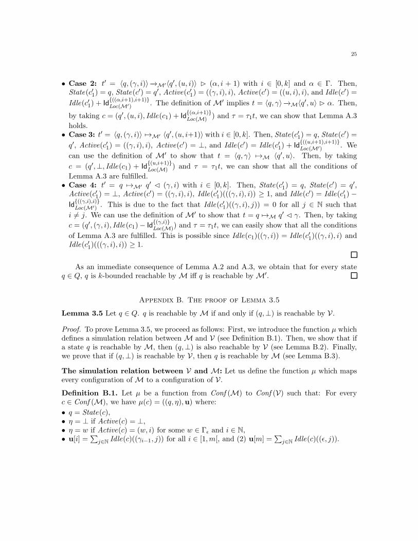
The Only if direction of Lemma 3.3: In the following, we show that if a state q isk-bounded reachable byM, then q is also reachable byM′.
Lemma A.2. If cinitMτ
==⇒∗T[0,k](M) c, then there is τ ′ ∈ (∆′)∗ such that cinitM′
τ ′==⇒∗
T (M′) c′ where
the configuration c′ ∈ Conf (M′) is defined as follows:
• State(c′) = State(c).• If Active(c) = ⊥, then Active(c′) = ⊥.• If Active(c) = (w, i) for some w ∈ Γǫ and i ∈ [0, k], then Active(c′) = ((w, i), i).• Idle(c′) is defined from Idle(c) as follows:(1) Idle(c′)(((w′, j′), j′)) = Idle(c)((w′, j′)) for all w′ ∈ Γǫ and j′ ∈ [0, k + 1], and(2) 0 otherwise.
23
Proof. First, we observe that cinitMτ
==⇒∗T[0,k](M) c implies Active(c) = ⊥ or Active(c) = (w, i)
for some w ∈ Γǫ and i ∈ [0, k] by definition. Let us assume that cinitMτ
==⇒n
T[0,k](M) c for some
n ∈ N. We proceed by induction on n.
Basis. n = 0. This implies that τ = ǫ and cinitM = c = (q0,⊥, Id{(γ0,0)}Loc(M)). Then, by taking
c′ = cinitM′ and τ ′ = ǫ, all the conditions of Lemma A.2 are satisfied.
Step. n > 0. Then there are c1 ∈ Conf (M), τ1 ∈ ∆∗, and t ∈ ∆ such that:
cinitMτ1===⇒
n−1T[0,k](M) c1
t−→ T[0,k](M) c (A.1)
We apply the induction hypothesis to the run cinitMτ1===⇒n−1
T[0,k](M) c1, and we obtain that
there are c′1 ∈ Conf (M′) and τ ′1 ∈ (∆′)∗ such that:
• cinitM′
τ ′1==⇒∗T (M′) c
′1.
• State(c′1) = State(c1).• If Active(c1) = ⊥, then Active(c′1) = ⊥.• If Active(c1) = (w, i) for some w ∈ Γǫ and i ∈ [0, k], then Active(c′1) = ((w, i), i).• The function Idle(c′1) is defined from Idle(c1) as follows:(1) Idle(c′1)(((w
′, j′), j′)) = Idle(c1)((w′, j′)) for all w′ ∈ Γǫ and j′ ∈ [0, k + 1], and
(2) 0 otherwise.
Since c1t−→ T[0,k](M) c, one of the following four cases holds:
• Case 1: t = 〈q, γ〉−→M〈q′, u〉 ⊲ ǫ. Then, there is i ∈ [0, k] such that State(c1) = q,
State(c) = q′, Active(c1) = (γ, i), Active(c) = (u, i), and Idle(c1) = Idle(c). Fromthe definition of M′, t′ = 〈q, (γ, i)〉−→M′〈q′, (u, i)〉 ⊲ ǫ. Moreover, we have State(c′1) =State(c1) = q and Active(c1) = ((γ, i), i). Then, by taking c′ = (q′, ((u, i), i), Idle (c′1))and τ ′ = τ ′1t
′, we can show that Lemma A.2 holds.• Case 2: t = 〈q, γ〉−→M〈q
′, u〉 ⊲ α with α ∈ Γ. Then, there is i ∈ [0, k] such thatState(c1) = q, State(c) = q′, Active(c1) = (γ, i), Active(c) = (u, i), and Idle(c) =
Idle(c1) + Id{(α,i+1)}Loc(M) . From the definition of M′, we have t′ = 〈q, (γ, i)〉−→M′〈q′, (u, i)〉
⊲ (α, i + 1). Then, by taking c′ = (q′, ((u, i), i), Idle (c′1) + Id{((α,i+1),i+1)}Loc(M′) ) and τ ′ = τ ′1t
′,
we can show that Lemma A.2 holds.• Case 3: t = 〈q, γ〉 7→M 〈q′, u〉. Then, there is i ∈ [0, k] such that State(c1) = q,
State(c) = q′, Active(c1) = (γ, i), Active(c) = ⊥, and Idle(c) = Idle(c1) + Id{(u,i+1)}Loc(M)
.
From the definition of M′, we have t′ = 〈q, (γ, i)〉 7→M′ 〈q′, (u, i + 1)〉. Then, by taking
c′ = (q′,⊥, Idle(c′1) + Id{((u,i+1),i+1)}Loc(M′) ) and τ ′ = τ ′1t
′, we can show that Lemma A.2 holds.
• Case 4: t = q 7→M q′ ⊳ γ with γ ∈ Γ. Then, there is i ∈ [0, k] such that State(c1) = q,State(c) = q′, Active(c1) = ⊥, Active(c) = (γ, i), Idle(c1)((γ, i)) ≥ 1, and Idle(c) =
Idle(c1) − Id{(γ,i)}Loc(M). From the definition of M′, we have t′ = q 7→M′ q′ ⊳ (γ, i). Then,
by taking c′ = (q′, ((γ, i), i), Idle (c′1) − Id{((γ,i),i)}Loc(M′) ) and τ ′ = τ ′1t
′, we can show that all
the conditions of Lemma A.2 are satisfied. This is possible since Idle(c′1)(((γ, i), i)) =Idle(c1)((γ, i)) ≥ 1.
24 M.F. ATIG, A. BOUAJJANI, AND S. QADEER
The If direction of Lemma 3.3 : In the following, we shows that if a state q is reachableby a computation ofM′, then q is k-bounded reachable byM.
Lemma A.3. If cinitM′τ ′==⇒∗
T (M′)c′, then there is τ ∈ ∆∗ such that cinitM
τ==⇒∗
T[0,k](M) c where
the configuration c ∈ Conf (M) is defined as follows:
• State(c) = State(c′).• If Active(c′) = ⊥, then Active(c) = ⊥.• If Active(c′) = ((w, i), i) for some w ∈ Γǫ and i ∈ [0, k], then Active(c) = (w, i).• Idle(c) is defined from Idle(c′) as follows:(1) Idle(c)((w′, j′)) = Idle(c′)(((w′, j′), j′)) for all w′ ∈ Γǫ and j′ ∈ [0, k + 1], and(2) 0 otherwise.
Proof. First, we observe that if cinitM′τ ′==⇒∗
T (M′)c′, then by Lemma A.1 Active(c′) = ⊥ or
Active(c′) = ((w, i), i) for some w ∈ Γǫ and i ∈ [0, k]. Let us assume that cinitM′τ ′==⇒n
T (M′) c′
for some n ∈ N. We proceed by induction on n.
Basis. n = 0. Then, τ ′ = ǫ and cinitM′ = c′ = (q0,⊥, Id{((γ0,0),0)}Loc(M′) ). By taking c = cinitM =
(q0,⊥, Id{(γ0,0)}Loc(M)) and τ = ǫ, we can show that all the conditions of Lemma A.3 are fulfilled.
Step. n > 1. Then, there are τ ′1 ∈ (∆′)∗, t′ ∈ ∆′, and c′1 ∈ Conf (M′) such that:
cinitM′
τ ′1===⇒n−1
T (M′) c′1
t′−→ T (M′) c′ (A.2)
We apply Lemma A.1 to cinitM′
τ ′1===⇒n−1
T (M′) c′1 and cinitM′
τ ′==⇒n
T (M′) c′, and we obtain that:
• Active(c′),Active(c′1) ∈(
{⊥} ∪ {((w, i), i) |w ∈ Γǫ, i ∈ [0, k]})
,• Idle(c′1)((ǫ, l)) = Idle(c′)((ǫ, l)) = 0 for all l ∈ N, and• Idle(c′1)((w
′, i′), j′)) = Idle(c′)((w′, i′), j′)) = 0 for all w′ ∈ Γǫ and i′ 6= j′.
We apply also the induction hypothesis to cinitM′
τ ′1===⇒n−1
T (M′) c′1, and we obtain that there
are τ1 ∈ ∆∗ and c1 ∈ Conf (M) such that:
• cinitMτ1==⇒∗
T[0,k](M) c1.
• State(c1) = State(c′1).• If Active(c′1) = ⊥, then Active(c1) = ⊥.• If Active(c′1) = ((w, i), i) for some w ∈ Γǫ and i ∈ [0, k], then Active(c1) = (w, i).• The function Idle(c1) is defined from Idle(c′1) as follows:(1) Idle(c1)((w
′, j′)) = Idle(c′1)(((w′, j′), j′)) for all w′ ∈ Γǫ and j′ ∈ [0, k + 1], and
(2) 0 otherwise.
On the other hand, c′1t′−→ T (M′) c
′ implies that one of the following four cases holds:
• Case 1: t′ = 〈q, (γ, i)〉−→M′〈q′, (u, i)〉 ⊲ ǫ with i ∈ [0, k]. Then, State(c′1) = q,State(c′) = q′, Active(c′1) = ((γ, i), i), Active(c′) = ((u, i), i), and Idle(c′1) = Idle(c′).We can use the definition ofM′ to show that t = 〈q, γ〉−→M〈q
′, u〉 ⊲ ǫ. Then, by takingc = (q′, (u, i), Idle(c1)) and τ = τ1t, we can show that Lemma A.3 holds.
25
• Case 2: t′ = 〈q, (γ, i)〉−→M′〈q′, (u, i)〉 ⊲ (α, i + 1) with i ∈ [0, k] and α ∈ Γ. Then,State(c′1) = q, State(c′) = q′, Active(c′1) = ((γ, i), i), Active(c′) = ((u, i), i), and Idle(c′) =
Idle(c′1) + Id{((α,i+1),i+1)}Loc(M′) . The definition ofM′ implies t = 〈q, γ〉−→M〈q
′, u〉 ⊲ α. Then,
by taking c = (q′, (u, i), Idle(c1) + Id{(α,i+1)}Loc(M) ) and τ = τ1t, we can show that Lemma A.3
holds.• Case 3: t′ = 〈q, (γ, i)〉 7→M′ 〈q′, (u, i+1)〉 with i ∈ [0, k]. Then, State(c′1) = q, State(c′) =
q′, Active(c′1) = ((γ, i), i), Active(c′) = ⊥, and Idle(c′) = Idle(c′1) + Id{((u,i+1),i+1)}Loc(M′) . We
can use the definition of M′ to show that t = 〈q, γ〉 7→M 〈q′, u〉. Then, by taking
c = (q′,⊥, Idle(c1) + Id{(u,i+1)}Loc(M) ) and τ = τ1t, we can show that all the conditions of
Lemma A.3 are fulfilled.• Case 4: t′ = q 7→M′ q′ ⊳ (γ, i) with i ∈ [0, k]. Then, State(c′1) = q, State(c′) = q′,Active(c′1) = ⊥, Active(c
′) = ((γ, i), i), Idle(c′1)(((γ, i), i)) ≥ 1, and Idle(c′) = Idle(c′1) −
Id{((γ,i),i)}Loc(M′) . This is due to the fact that Idle(c′1)((γ, i), j)) = 0 for all j ∈ N such that
i 6= j. We can use the definition ofM′ to show that t = q 7→M q′ ⊳ γ. Then, by taking
c = (q′, (γ, i), Idle(c1)− Id{(γ,i)}Loc(M)) and τ = τ1t, we can easily show that all the conditions
of Lemma A.3 are fulfilled. This is possible since Idle(c1)((γ, i)) = Idle(c′1)((γ, i), i) andIdle(c′1)(((γ, i), i)) ≥ 1.
As an immediate consequence of Lemma A.2 and A.3, we obtain that for every stateq ∈ Q, q is k-bounded reachable byM iff q is reachable byM′.
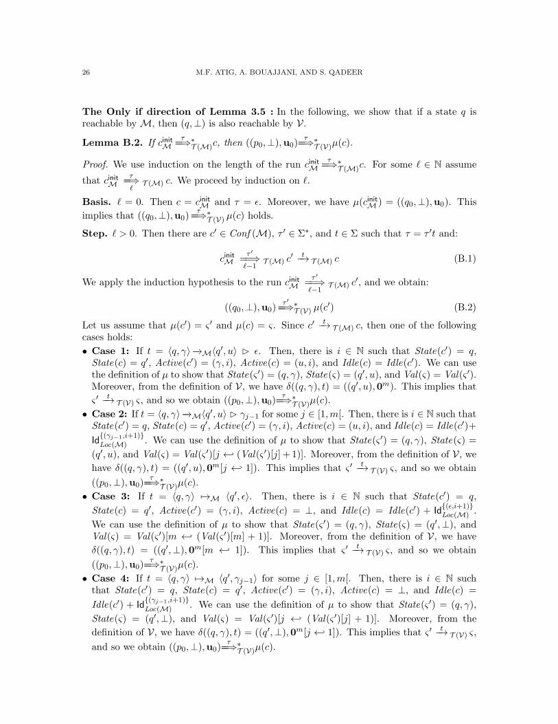
Appendix B. The proof of Lemma 3.5
Lemma 3.5 Let q ∈ Q. q is reachable byM if and only if (q,⊥) is reachable by V.
Proof. To prove Lemma 3.5, we proceed as follows: First, we introduce the function µ whichdefines a simulation relation betweenM and V (see Definition B.1). Then, we show that ifa state q is reachable byM, then (q,⊥) is also reachable by V (see Lemma B.2). Finally,we prove that if (q,⊥) is reachable by V, then q is reachable byM (see Lemma B.3).
The simulation relation between V and M: Let us define the function µ which mapsevery configuration ofM to a configuration of V.
Definition B.1. Let µ be a function from Conf (M) to Conf (V) such that: For everyc ∈ Conf (M), we have µ(c) = ((q, η),u) where:
• q = State(c),• η = ⊥ if Active(c) = ⊥,• η = w if Active(c) = (w, i) for some w ∈ Γǫ and i ∈ N,• u[i] =
∑
j∈N Idle(c)((γi−1, j)) for all i ∈ [1,m[, and (2) u[m] =∑
j∈N Idle(c)((ǫ, j)).
26 M.F. ATIG, A. BOUAJJANI, AND S. QADEER
The Only if direction of Lemma 3.5 : In the following, we show that if a state q isreachable byM, then (q,⊥) is also reachable by V.
Lemma B.2. If cinitMτ
==⇒∗T (M)c, then ((p0,⊥),u0)
τ==⇒∗
T (V)µ(c).
Proof. We use induction on the length of the run cinitMτ
==⇒∗T (M)c. For some ℓ ∈ N assume
that cinitMτ
==⇒ℓ
T (M) c. We proceed by induction on ℓ.
Basis. ℓ = 0. Then c = cinitM and τ = ǫ. Moreover, we have µ(cinitM ) = ((q0,⊥),u0). This
implies that ((q0,⊥),u0)τ
==⇒∗T (V) µ(c) holds.
Step. ℓ > 0. Then there are c′ ∈ Conf (M), τ ′ ∈ Σ∗, and t ∈ Σ such that τ = τ ′t and:
cinitMτ ′
==⇒ℓ−1
T (M) c′ t−→ T (M) c (B.1)
We apply the induction hypothesis to the run cinitMτ ′
==⇒ℓ−1
T (M) c′, and we obtain:
((q0,⊥),u0)τ ′==⇒∗
T (V) µ(c′) (B.2)
Let us assume that µ(c′) = ς ′ and µ(c) = ς. Since c′ t−→ T (M) c, then one of the followingcases holds:
• Case 1: If t = 〈q, γ〉−→M〈q′, u〉 ⊲ ǫ. Then, there is i ∈ N such that State(c′) = q,
State(c) = q′, Active(c′) = (γ, i), Active(c) = (u, i), and Idle(c) = Idle(c′). We can usethe definition of µ to show that State(ς ′) = (q, γ), State(ς) = (q′, u), and Val(ς) = Val(ς ′).Moreover, from the definition of V, we have δ((q, γ), t) = ((q′, u),0m). This implies that
ς ′ t−→ T (V) ς, and so we obtain ((p0,⊥),u0)τ
==⇒∗T (V)µ(c).
• Case 2: If t = 〈q, γ〉−→M〈q′, u〉 ⊲ γj−1 for some j ∈ [1,m[. Then, there is i ∈ N such that
State(c′) = q, State(c) = q′, Active(c′) = (γ, i), Active(c) = (u, i), and Idle(c) = Idle(c′)+
Id{(γj−1,i+1)}Loc(M) . We can use the definition of µ to show that State(ς ′) = (q, γ), State(ς) =
(q′, u), and Val(ς) = Val(ς ′)[j ← (Val(ς ′)[j] + 1)]. Moreover, from the definition of V, we
have δ((q, γ), t) = ((q′, u),0m[j ← 1]). This implies that ς ′ t−→ T (V) ς, and so we obtain
((p0,⊥),u0)τ
==⇒∗T (V)µ(c).
• Case 3: If t = 〈q, γ〉 7→M 〈q′, ǫ〉. Then, there is i ∈ N such that State(c′) = q,
State(c) = q′, Active(c′) = (γ, i), Active(c) = ⊥, and Idle(c) = Idle(c′) + Id{(ǫ,i+1)}Loc(M) .
We can use the definition of µ to show that State(ς ′) = (q, γ), State(ς) = (q′,⊥), andVal(ς) = Val(ς ′)[m ← (Val(ς ′)[m] + 1)]. Moreover, from the definition of V, we have
δ((q, γ), t) = ((q′,⊥),0m[m ← 1]). This implies that ς ′ t−→ T (V) ς, and so we obtain
((p0,⊥),u0)τ
==⇒∗T (V)µ(c).
• Case 4: If t = 〈q, γ〉 7→M 〈q′, γj−1〉 for some j ∈ [1,m[. Then, there is i ∈ N suchthat State(c′) = q, State(c) = q′, Active(c′) = (γ, i), Active(c) = ⊥, and Idle(c) =
Idle(c′) + Id{(γj−1,i+1)}Loc(M) . We can use the definition of µ to show that State(ς ′) = (q, γ),
State(ς) = (q′,⊥), and Val(ς) = Val(ς ′)[j ← (Val(ς ′)[j] + 1)]. Moreover, from the
definition of V, we have δ((q, γ), t) = ((q′,⊥),0m[j ← 1]). This implies that ς ′ t−→ T (V) ς,
and so we obtain ((p0,⊥),u0)τ
==⇒∗T (V)µ(c).
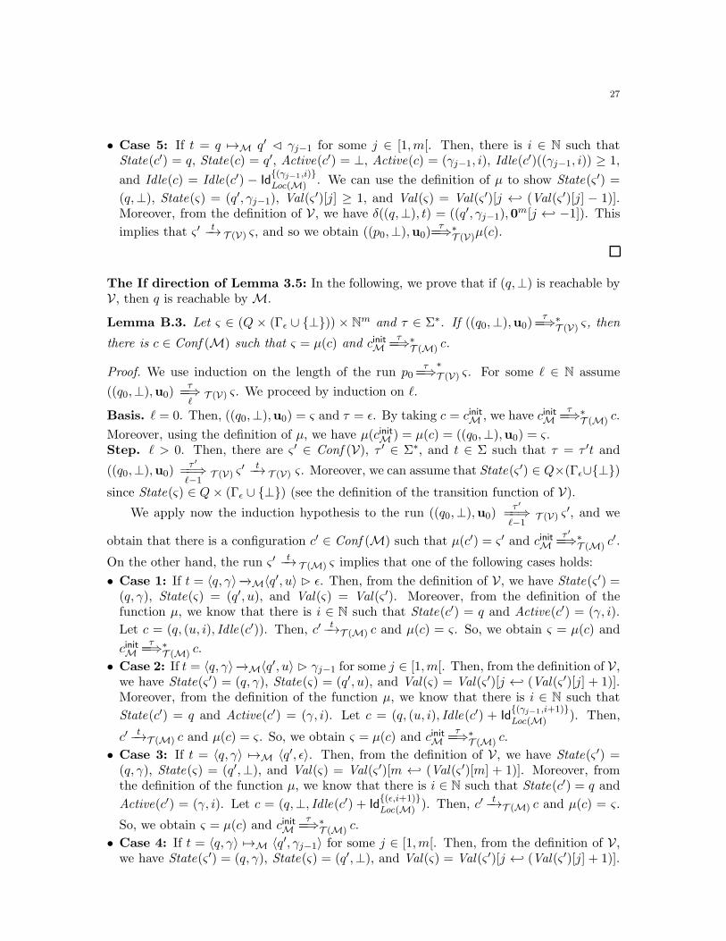
27
• Case 5: If t = q 7→M q′ ⊳ γj−1 for some j ∈ [1,m[. Then, there is i ∈ N such thatState(c′) = q, State(c) = q′, Active(c′) = ⊥, Active(c) = (γj−1, i), Idle(c
′)((γj−1, i)) ≥ 1,
and Idle(c) = Idle(c′) − Id{(γj−1,i)}Loc(M) . We can use the definition of µ to show State(ς ′) =
(q,⊥), State(ς) = (q′, γj−1), Val(ς′)[j] ≥ 1, and Val(ς) = Val(ς ′)[j ← (Val(ς ′)[j] − 1)].
Moreover, from the definition of V, we have δ((q,⊥), t) = ((q′, γj−1),0m[j ← −1]). This
implies that ς ′ t−→ T (V) ς, and so we obtain ((p0,⊥),u0)τ
==⇒∗T (V)µ(c).
The If direction of Lemma 3.5: In the following, we prove that if (q,⊥) is reachable byV, then q is reachable byM.
Lemma B.3. Let ς ∈ (Q × (Γǫ ∪ {⊥})) × Nm and τ ∈ Σ∗. If ((q0,⊥),u0)
τ==⇒∗
T (V) ς, then
there is c ∈ Conf (M) such that ς = µ(c) and cinitMτ
==⇒∗T (M) c.
Proof. We use induction on the length of the run p0τ
==⇒∗
T (V) ς. For some ℓ ∈ N assume
((q0,⊥),u0)τ
==⇒ℓ
T (V) ς. We proceed by induction on ℓ.
Basis. ℓ = 0. Then, ((q0,⊥),u0) = ς and τ = ǫ. By taking c = cinitM , we have cinitMτ
==⇒∗T (M) c.
Moreover, using the definition of µ, we have µ(cinitM ) = µ(c) = ((q0,⊥),u0) = ς.Step. ℓ > 0. Then, there are ς ′ ∈ Conf (V), τ ′ ∈ Σ∗, and t ∈ Σ such that τ = τ ′t and
((q0,⊥),u0)τ ′
==⇒ℓ−1
T (V) ς′ t−→ T (V) ς. Moreover, we can assume that State(ς ′) ∈ Q×(Γǫ∪{⊥})
since State(ς) ∈ Q× (Γǫ ∪ {⊥}) (see the definition of the transition function of V).
We apply now the induction hypothesis to the run ((q0,⊥),u0)τ ′
==⇒ℓ−1
T (V) ς′, and we
obtain that there is a configuration c′ ∈ Conf (M) such that µ(c′) = ς ′ and cinitMτ ′==⇒∗
T (M) c′.
On the other hand, the run ς ′ t−→ T (M) ς implies that one of the following cases holds:
• Case 1: If t = 〈q, γ〉−→M〈q′, u〉 ⊲ ǫ. Then, from the definition of V, we have State(ς ′) =
(q, γ), State(ς) = (q′, u), and Val(ς) = Val(ς ′). Moreover, from the definition of thefunction µ, we know that there is i ∈ N such that State(c′) = q and Active(c′) = (γ, i).
Let c = (q, (u, i), Idle(c′)). Then, c′ t−→T (M) c and µ(c) = ς. So, we obtain ς = µ(c) and
cinitMτ
==⇒∗T (M) c.
• Case 2: If t = 〈q, γ〉−→M〈q′, u〉 ⊲ γj−1 for some j ∈ [1,m[. Then, from the definition of V,
we have State(ς ′) = (q, γ), State(ς) = (q′, u), and Val(ς) = Val(ς ′)[j ← (Val(ς ′)[j] + 1)].Moreover, from the definition of the function µ, we know that there is i ∈ N such that
State(c′) = q and Active(c′) = (γ, i). Let c = (q, (u, i), Idle(c′) + Id{(γj−1,i+1)}Loc(M) ). Then,
c′ t−→T (M) c and µ(c) = ς. So, we obtain ς = µ(c) and cinitMτ
==⇒∗T (M) c.
• Case 3: If t = 〈q, γ〉 7→M 〈q′, ǫ〉. Then, from the definition of V, we have State(ς ′) =(q, γ), State(ς) = (q′,⊥), and Val(ς) = Val(ς ′)[m ← (Val(ς ′)[m] + 1)]. Moreover, fromthe definition of the function µ, we know that there is i ∈ N such that State(c′) = q and
Active(c′) = (γ, i). Let c = (q,⊥, Idle(c′) + Id{(ǫ,i+1)}Loc(M) ). Then, c′ t−→T (M) c and µ(c) = ς.
So, we obtain ς = µ(c) and cinitMτ
==⇒∗T (M) c.
• Case 4: If t = 〈q, γ〉 7→M 〈q′, γj−1〉 for some j ∈ [1,m[. Then, from the definition of V,
we have State(ς ′) = (q, γ), State(ς) = (q′,⊥), and Val(ς) = Val(ς ′)[j ← (Val(ς ′)[j] + 1)].
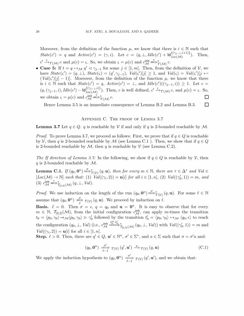
28 M.F. ATIG, A. BOUAJJANI, AND S. QADEER
Moreover, from the definition of the function µ, we know that there is i ∈ N such that
State(c′) = q and Active(c′) = (γ, i). Let c = (q,⊥, Idle(c′) + Id{(γj−1,i+1)}
Loc(M)). Then,
c′ t−→T (M) c and µ(c) = ς. So, we obtain ς = µ(c) and cinitMτ
==⇒∗T (M) c.
• Case 5: If t = q 7→M q′ ⊳ γj−1 for some j ∈ [1,m[. Then, from the definition of V, wehave State(ς ′) = (q,⊥), State(ς) = (q′, γj−1), Val(ς
′)[j] ≥ 1, and Val(ς) = Val(ς ′)[j ←(Val(ς ′)[j] − 1)]. Moreover, from the definition of the function µ, we know that thereis i ∈ N such that State(c′) = q, Active(c′) = ⊥, and Idle(c′)((γj−1, i)) ≥ 1. Let c =
(q, (γj−1, i), Idle(c′)− Id
{(γj−1,i)}Loc(M) ). Then, c is well defined, c′ t−→T (M) c, and µ(c) = ς. So,
we obtain ς = µ(c) and cinitMτ
==⇒∗T (M) c.
Hence Lemma 3.5 is an immediate consequence of Lemma B.2 and Lemma B.3.
Appendix C. The proof of Lemma 3.7
Lemma 3.7 Let q ∈ Q. q is reachable by V if and only if q is 2-bounded reachable byM.
Proof. To prove Lemma 3.7, we proceed as follows: First, we prove that if q ∈ Q is reachableby V, then q is 2-bounded reachable byM (see Lemma C.1 ). Then, we show that if q ∈ Qis 2-bounded reachable byM, then q is reachable by V (see Lemma C.2).
The If direction of Lemma 3.7: In the following, we show if q ∈ Q is reachable by V, thenq is 2-bounded reachable byM.
Lemma C.1. If (q0,0n)
σ==⇒∗
T (V) (q,u), then for every m ∈ N, there are τ ∈ ∆∗ and Val ∈
[Loc(M)→ N] such that: (1) Val((γi, 2)) = u[i] for all i ∈ [1, n], (2) Val((γ′0, 1)) = m, and
(3) cinitMτ
==⇒∗T[0,2](M) (q,⊥,Val).
Proof. We use induction on the length of the run (q0,0n)
σ==⇒∗
T (V) (q,u). For some ℓ ∈ N
assume that (q0,0n)
σ==⇒ℓ
T (V) (q,u). We proceed by induction on ℓ.
Basis. ℓ = 0. Then σ = ǫ, q = q0 and u = 0n. It is easy to observe that for everym ∈ N, T[0,2](M), from the initial configuration cinitM , can apply m-times the transitiont0 = 〈p0, γ0〉−→M〈p0, γ0〉 ⊲ γ′0 followed by the transition t′0 = 〈p0, γ0〉 7→M 〈q0, ǫ〉 to reach
the configuration (q0,⊥,Val) (i.e., cinitM
tm0 ·t′0===⇒∗T[0,2](M) (q0,⊥,Val)) with Val((γ′0, 1)) = m and
Val((γi, 2)) = u[i] for all i ∈ [1, n].Step. ℓ > 0. Then, there are q′ ∈ Q, u′ ∈ N
n, σ′ ∈ Σ∗, and a ∈ Σ such that σ = σ′a and:
(q0,0n)
σ′
==⇒ℓ−1
T (V) (q′,u′) a−→ T (V) (q,u) (C.1)
We apply the induction hypothesis to (q0,0n)
σ′
==⇒ℓ−1
T (V) (q′,u′), and we obtain that:
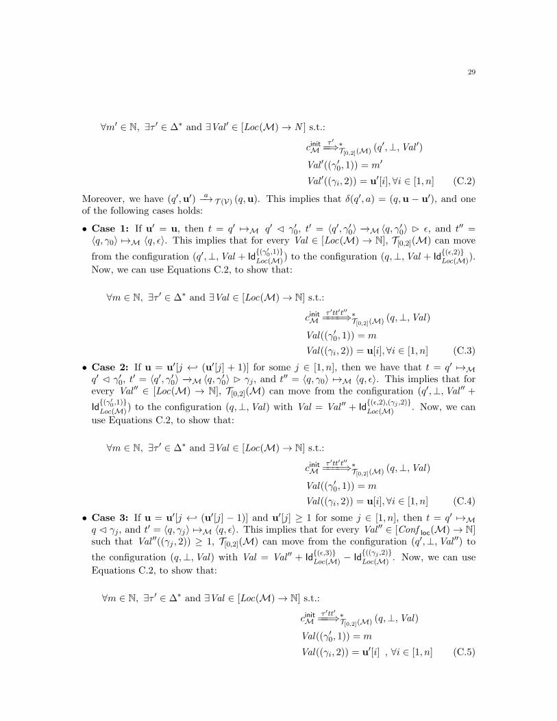
29
∀m′ ∈ N, ∃τ ′ ∈ ∆∗ and ∃Val ′ ∈ [Loc(M)→ N ] s.t.:
cinitMτ ′==⇒∗
T[0,2](M) (q′,⊥,Val ′)
Val ′((γ′0, 1)) = m′
Val ′((γi, 2)) = u′[i],∀i ∈ [1, n] (C.2)
Moreover, we have (q′,u′) a−→ T (V) (q,u). This implies that δ(q′, a) = (q,u − u′), and oneof the following cases holds:
• Case 1: If u′ = u, then t = q′ 7→M q′ ⊳ γ′0, t′ = 〈q′, γ′0〉 −→M 〈q, γ
′0〉 ⊲ ǫ, and t′′ =
〈q, γ0〉 7→M 〈q, ǫ〉. This implies that for every Val ∈ [Loc(M) → N], T[0,2](M) can move
from the configuration (q′,⊥,Val + Id{(γ′
0,1)}
Loc(M)) to the configuration (q,⊥,Val + Id{(ǫ,2)}Loc(M)).
Now, we can use Equations C.2, to show that:
∀m ∈ N, ∃τ ′ ∈ ∆∗ and ∃Val ∈ [Loc(M)→ N] s.t.:
cinitMτ ′tt′t′′====⇒∗
T[0,2](M) (q,⊥,Val)
Val((γ′0, 1)) = m
Val((γi, 2)) = u[i],∀i ∈ [1, n] (C.3)
• Case 2: If u = u′[j ← (u′[j] + 1)] for some j ∈ [1, n], then we have that t = q′ 7→M
q′ ⊳ γ′0, t′ = 〈q′, γ′0〉 −→M 〈q, γ
′0〉 ⊲ γj, and t′′ = 〈q, γ0〉 7→M 〈q, ǫ〉. This implies that for
every Val ′′ ∈ [Loc(M) → N], T[0,2](M) can move from the configuration (q′,⊥,Val ′′ +
Id{(γ′
0,1)}
Loc(M)) to the configuration (q,⊥,Val) with Val = Val ′′ + Id{(ǫ,2),(γj ,2)}Loc(M) . Now, we can
use Equations C.2, to show that:
∀m ∈ N, ∃τ ′ ∈ ∆∗ and ∃Val ∈ [Loc(M)→ N] s.t.:
cinitMτ ′tt′t′′====⇒∗
T[0,2](M) (q,⊥,Val)
Val((γ′0, 1)) = m
Val((γi, 2)) = u[i],∀i ∈ [1, n] (C.4)
• Case 3: If u = u′[j ← (u′[j] − 1)] and u′[j] ≥ 1 for some j ∈ [1, n], then t = q′ 7→M
q ⊳ γj, and t′ = 〈q, γj〉 7→M 〈q, ǫ〉. This implies that for every Val ′′ ∈ [Conf loc(M)→ N]such that Val ′′((γj , 2)) ≥ 1, T[0,2](M) can move from the configuration (q′,⊥,Val ′′) to
the configuration (q,⊥,Val) with Val = Val ′′ + Id{(ǫ,3)}Loc(M) − Id
{((γj ,2)}Loc(M) . Now, we can use
Equations C.2, to show that:
∀m ∈ N, ∃τ ′ ∈ ∆∗ and ∃Val ∈ [Loc(M)→ N] s.t.:
cinitMτ ′tt′===⇒∗
T[0,2](M) (q,⊥,Val)
Val((γ′0, 1)) = m
Val((γi, 2)) = u′[i] , ∀i ∈ [1, n] (C.5)
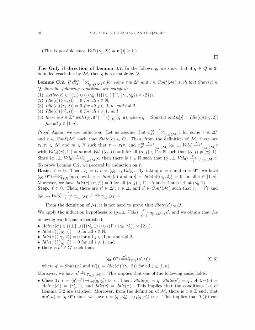
30 M.F. ATIG, A. BOUAJJANI, AND S. QADEER
(This is possible since Val ′((γj , 2)) = u′[j] ≥ 1.)
The Only if direction of Lemma 3.7: In the following, we show that if q ∈ Q is 2-bounded reachable byM, then q is reachable by V.
Lemma C.2. If cinitMτ
==⇒∗T[0,2](M) c for some τ ∈ ∆∗ and c ∈ Conf (M) such that State(c) ∈
Q, then the following conditions are satisfied:
(1) Active(c) ∈ ({⊥} ∪ ({(γ′0, 1)}) ∪ ((Γ \ {γ0, γ′0})× {2})),
(2) Idle(c)((γ0, i)) = 0 for all i ∈ N,(3) Idle(c)((γj , i)) = 0 for all j ∈ [1, n] and i 6= 2,(4) Idle(c)((γ′0, i)) = 0 for all i 6= 1, and
(5) there is σ ∈ Σ∗ with (q0,0n)
σ==⇒∗
T (V) (q,u), where q = State(c) and u[j] = Idle(c)((γj , 2))
for all j ∈ [1, n].
Proof. Again, we use induction. Let us assume that cinitMτ
==⇒∗T[0,2](M) c for some τ ∈ ∆∗
and c ∈ Conf (M) such that State(c) ∈ Q. Then, from the definition of M, there are
τ1, τ2 ∈ ∆∗ and m ∈ N such that τ = τ1τ2 and cinitMτ1==⇒∗
T[0,2](M) (q0,⊥,Val0)τ2==⇒∗
T[0,2](M)c
with Val0((γ′0, 1)) = m and Val0((α, j)) = 0 for all (α, j) ∈ Γ×N such that (α, j) 6= (γ′0, 1).
Since (q0,⊥,Val0)τ2==⇒∗
T[0,2](M)c, then there is ℓ ∈ N such that (q0,⊥,Val0)τ2==⇒ℓ
T[0,2](M) c.
To prove Lemma C.2, we proceed by induction on ℓ.Basis. ℓ = 0. Then, τ2 = ǫ, c = (q0,⊥,Val0). By taking σ = ǫ and u = 0n, we have
(q0,0n)
σ==⇒∗
T (V) (q,u) with q = State(c) and u[i] = Idle(c)((γi, 2)) = 0 for all i ∈ [1, n].
Moreover, we have Idle(c)((α, j)) = 0 for all (α, j) ∈ Γ× N such that (α, j) 6= (γ′0, 1).Step. ℓ > 0. Then, there are τ ′ ∈ ∆∗, t ∈ ∆, and c′ ∈ Conf (M) such that τ2 = τ ′t and
(q0,⊥,Val 0)τ ′
==⇒ℓ−1
T[0,2](M) c′ t−→ T[0,2](M) c.
From the definition ofM, it is not hard to prove that State(c′) ∈ Q.
We apply the induction hypothesis to (q0,⊥,Val0)τ ′
==⇒ℓ−1
T[0,2](M) c′, and we obtain that the
following conditions are satisfied:
• Active(c′) ∈ ({⊥} ∪ ({(γ′0, 1)}) ∪ ((Γ \ {γ0, γ′0})× {2})),
• Idle(c′)((γ0, i)) = 0 for all i ∈ N,• Idle(c′)((γj , i)) = 0 for all j ∈ [1, n] and i 6= 2,• Idle(c′)((γ′0, i)) = 0 for all i 6= 1, and• there is σ′ ∈ Σ∗ such that:
(q0,0n)
σ′
==⇒∗T (V) (q
′,u′) (C.6)
where q′ = State(c′) and u′[j] = Idle(c′)((γj , 2)) for all j ∈ [1, n].
Moreover, we have c′ t−→ T[0,2](M) c. This implies that one of the following cases holds:
• Case 1: t = 〈q′, γ′0〉−→M〈q, γ′0〉 ⊲ ǫ. Then, State(c) = q, State(c′) = q′, Active(c) =
Active(c′) = (γ′0, 1), and Idle(c) = Idle(c′). This implies that the conditions 1-4 ofLemma C.2 are satisfied. Moreover, from the definition of M, there is a ∈ Σ such thatδ(q′, a) = (q,0n) since we have t = 〈q′, γ′0〉−→M〈q, γ
′0〉 ⊲ ǫ. This implies that T (V) can
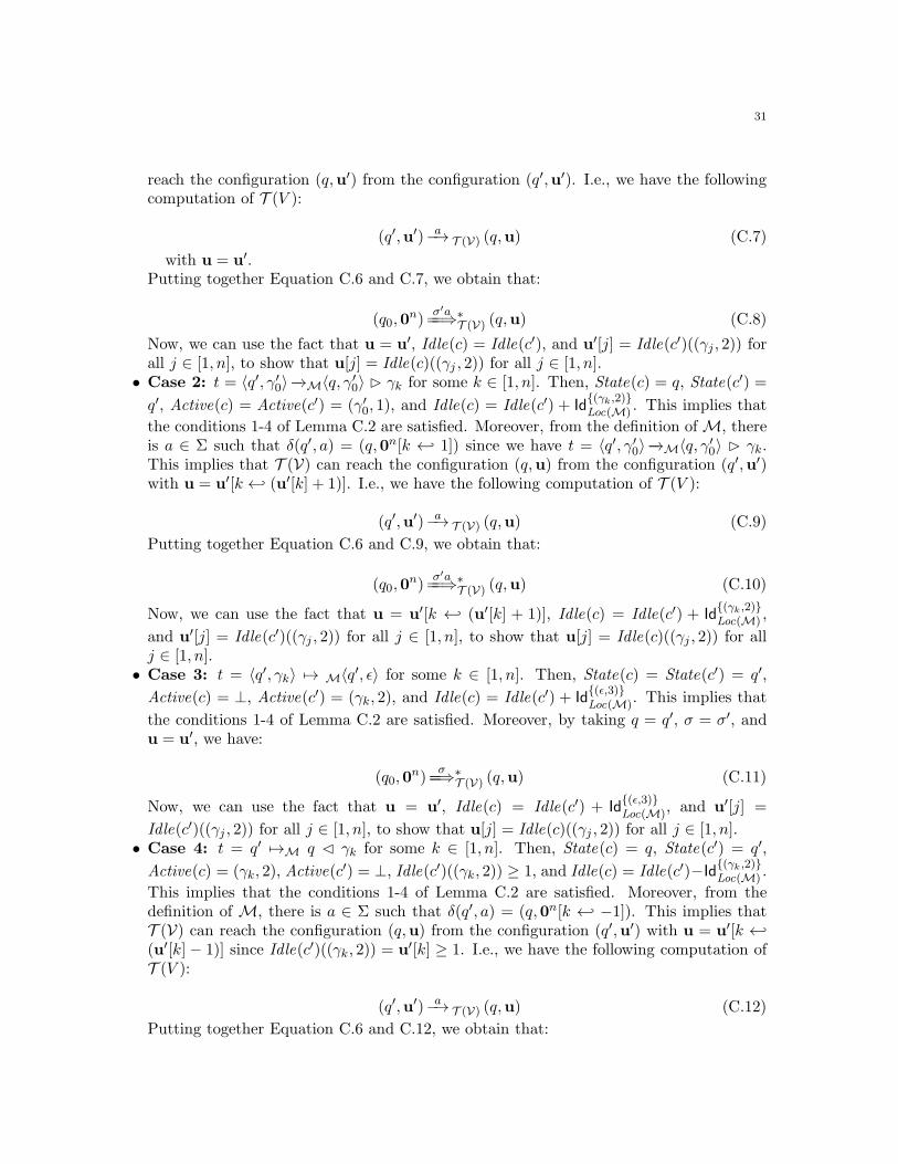
31
reach the configuration (q,u′) from the configuration (q′,u′). I.e., we have the followingcomputation of T (V ):
(q′,u′) a−→ T (V) (q,u) (C.7)
with u = u′.Putting together Equation C.6 and C.7, we obtain that:
(q0,0n)
σ′a==⇒∗
T (V) (q,u) (C.8)
Now, we can use the fact that u = u′, Idle(c) = Idle(c′), and u′[j] = Idle(c′)((γj , 2)) forall j ∈ [1, n], to show that u[j] = Idle(c)((γj , 2)) for all j ∈ [1, n].• Case 2: t = 〈q′, γ′0〉−→M〈q, γ
′0〉 ⊲ γk for some k ∈ [1, n]. Then, State(c) = q, State(c′) =
q′, Active(c) = Active(c′) = (γ′0, 1), and Idle(c) = Idle(c′) + Id{(γk ,2)}Loc(M) . This implies that
the conditions 1-4 of Lemma C.2 are satisfied. Moreover, from the definition ofM, thereis a ∈ Σ such that δ(q′, a) = (q,0n[k ← 1]) since we have t = 〈q′, γ′0〉−→M〈q, γ
′0〉 ⊲ γk.
This implies that T (V) can reach the configuration (q,u) from the configuration (q′,u′)with u = u′[k ← (u′[k] + 1)]. I.e., we have the following computation of T (V ):
(q′,u′) a−→ T (V) (q,u) (C.9)
Putting together Equation C.6 and C.9, we obtain that:
(q0,0n)
σ′a==⇒∗
T (V) (q,u) (C.10)
Now, we can use the fact that u = u′[k ← (u′[k] + 1)], Idle(c) = Idle(c′) + Id{(γk ,2)}Loc(M) ,
and u′[j] = Idle(c′)((γj , 2)) for all j ∈ [1, n], to show that u[j] = Idle(c)((γj , 2)) for allj ∈ [1, n].• Case 3: t = 〈q′, γk〉 7→ M〈q
′, ǫ〉 for some k ∈ [1, n]. Then, State(c) = State(c′) = q′,
Active(c) = ⊥, Active(c′) = (γk, 2), and Idle(c) = Idle(c′) + Id{(ǫ,3)}Loc(M)
. This implies that
the conditions 1-4 of Lemma C.2 are satisfied. Moreover, by taking q = q′, σ = σ′, andu = u′, we have:
(q0,0n)
σ==⇒∗
T (V) (q,u) (C.11)
Now, we can use the fact that u = u′, Idle(c) = Idle(c′) + Id{(ǫ,3)}Loc(M)
, and u′[j] =
Idle(c′)((γj , 2)) for all j ∈ [1, n], to show that u[j] = Idle(c)((γj , 2)) for all j ∈ [1, n].• Case 4: t = q′ 7→M q ⊳ γk for some k ∈ [1, n]. Then, State(c) = q, State(c′) = q′,
Active(c) = (γk, 2), Active(c′) = ⊥, Idle(c′)((γk, 2)) ≥ 1, and Idle(c) = Idle(c′)−Id
{(γk ,2)}Loc(M) .
This implies that the conditions 1-4 of Lemma C.2 are satisfied. Moreover, from thedefinition of M, there is a ∈ Σ such that δ(q′, a) = (q,0n[k ← −1]). This implies thatT (V) can reach the configuration (q,u) from the configuration (q′,u′) with u = u′[k ←(u′[k]− 1)] since Idle(c′)((γk, 2)) = u′[k] ≥ 1. I.e., we have the following computation ofT (V ):
(q′,u′) a−→ T (V) (q,u) (C.12)
Putting together Equation C.6 and C.12, we obtain that:
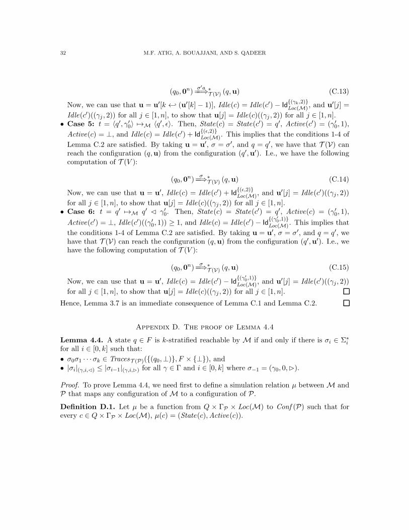
32 M.F. ATIG, A. BOUAJJANI, AND S. QADEER
(q0,0n)
σ′a==⇒∗
T (V) (q,u) (C.13)
Now, we can use that u = u′[k ← (u′[k]− 1)], Idle(c) = Idle(c′) − Id{(γk ,2)}Loc(M) , and u′[j] =
Idle(c′)((γj , 2)) for all j ∈ [1, n], to show that u[j] = Idle(c)((γj , 2)) for all j ∈ [1, n].• Case 5: t = 〈q′, γ′0〉 7→M 〈q′, ǫ〉. Then, State(c) = State(c′) = q′, Active(c′) = (γ′0, 1),
Active(c) = ⊥, and Idle(c) = Idle(c′) + Id{(ǫ,2)}Loc(M). This implies that the conditions 1-4 of
Lemma C.2 are satisfied. By taking u = u′, σ = σ′, and q = q′, we have that T (V) canreach the configuration (q,u) from the configuration (q′,u′). I.e., we have the followingcomputation of T (V ):
(q0,0n)
σ==⇒∗
T (V) (q,u) (C.14)
Now, we can use that u = u′, Idle(c) = Idle(c′) + Id{(ǫ,2)}Loc(M), and u′[j] = Idle(c′)((γj , 2))
for all j ∈ [1, n], to show that u[j] = Idle(c)((γj , 2)) for all j ∈ [1, n].• Case 6: t = q′ 7→M q′ ⊳ γ′0. Then, State(c) = State(c′) = q′, Active(c) = (γ′0, 1),
Active(c′) = ⊥, Idle(c′)((γ′0, 1)) ≥ 1, and Idle(c) = Idle(c′)− Id{(γ′
0,1)}
Loc(M) . This implies that
the conditions 1-4 of Lemma C.2 are satisfied. By taking u = u′, σ = σ′, and q = q′, wehave that T (V) can reach the configuration (q,u) from the configuration (q′,u′). I.e., wehave the following computation of T (V ):
(q0,0n)
σ==⇒∗
T (V) (q,u) (C.15)
Now, we can use that u = u′, Idle(c) = Idle(c′) − Id{(γ′
0,1)}
Loc(M), and u′[j] = Idle(c′)((γj , 2))
for all j ∈ [1, n], to show that u[j] = Idle(c)((γj , 2)) for all j ∈ [1, n].
Hence, Lemma 3.7 is an immediate consequence of Lemma C.1 and Lemma C.2.
Appendix D. The proof of Lemma 4.4
Lemma 4.4. A state q ∈ F is k-stratified reachable by M if and only if there is σi ∈ Σ∗i
for all i ∈ [0, k] such that:
• σ0σ1 · · · σk ∈ TracesT (P)({(q0,⊥)}, F × {⊥}), and• |σi|(γ,i,⊳) ≤ |σi−1|(γ,i,⊲) for all γ ∈ Γ and i ∈ [0, k] where σ−1 = (γ0, 0,⊲).
Proof. To prove Lemma 4.4, we need first to define a simulation relation µ betweenM andP that maps any configuration ofM to a configuration of P.
Definition D.1. Let µ be a function from Q × ΓP × Loc(M) to Conf (P) such that forevery c ∈ Q× ΓP × Loc(M), µ(c) = (State(c),Active(c)).
33
The Only if direction of Lemma 4.4: In the following, we show that if there is a state q ∈ Fsuch that q is k-stratified reachable byM, then there is σi ∈ Σ∗
i for all i ∈ [0, k] such thatσ0σ1 · · · σk ∈ TracesT (P)({(q0,⊥)}, F × {⊥}), and |σi|(γ,i,⊳) ≤ |σi−1|(γ,i,⊲) for all γ ∈ Γ andi ∈ [0, k] where σ−1 = (γ0, 0,⊲).
To this aim, we first prove that if there is a run cτi==⇒∗
T{i}(M) c′ ( where M executes
only threads with switch number i ∈ [0, k]), then there is a run µ(c)σi==⇒∗
T (P) µ(c′) of P such
that: (1) σi ∈ Σ∗i , (2) the number of occurrences of (γ, i,⊳) in σi is equal to the number of
activated threads byM with local configuration (γ, i), and (3) the number of created/addedthreads by M with local configuration (γ, i + 1) is equal to the number of occurrence of(γ, i+ 1,⊲) in σi.
Lemma D.2. For every i ∈ [0, k], and c, c′ ∈(
Q× ΓP × Loc(M))
, if there is τi ∈ ∆∗ such
that cτi==⇒∗
T{i}(M) c′, then there is σi ∈ Σ∗
i such that:
(1) µ(c)σi==⇒∗
T (P) µ(c′).
(2) Idle(c)((α, i)) ≥ |σi|(α,i,⊳) for all α ∈ Γǫ.
(3) Idle(c′)((α, i)) = Idle(c)((α, i))−|σi |(α,i,⊳) and Idle(c′)((α, i+1)) = Idle(c)((α, i+1))+|σi|(α,i+1,⊲) for all α ∈ Γǫ.
(4) Idle(c′)((α, j)) = Idle(c)((α, j)) for all (α, j) ∈ Γǫ × [0, k + 1] such that j /∈ {i, i + 1}.
Proof. Assume that cτi==⇒ℓ
T{i}(M) c′ for some ℓ ∈ N. We proceed by induction on ℓ.
Basis. ℓ = 0. Then, τi = ǫ and c = c′. By taking σi = ǫ, we have all the conditions ofLemma D.2 are fulfilled.Step. ℓ > 0. Then there are τ ′i ∈ ∆∗, t ∈ ∆, c′′ ∈
(
Q× ΓP × Loc(M))
such that:
cτ ′i==⇒ℓ−1
T{i}(M) c′′ t−→ T{i}(M) c
′ (D.1)
We apply the induction hypothesis to the run cτ ′i==⇒ℓ−1
T{i}(M) c′′, and we obtain that there
is σ′i ∈ Σ∗
i such that:
• µ(c)σ′i==⇒∗T (P) µ(c
′′).
• Idle(c)((α, i)) ≥ |σ′i|(α,i,⊳) for all α ∈ Γǫ.
• Idle(c′′)((α, i)) = Idle(c)((α, i))− |σ′i|(α,i,⊳) and Idle(c′′)((α, i+1)) = Idle(c)((α, i+1))+
|σ′i|(α,i+1,⊲) for all α ∈ Γǫ.
• Idle(c′′)((α, j)) = Idle(c)((α, j)) for all (α, j) ∈ Γǫ × [0, k + 1] such that j /∈ {i, i+ 1}.
Since we have c′′ t−→ T{i}(M) c′, one of the followings cases holds:
• Case 1: t = 〈q′′, γ〉−→M〈q′, u〉 ⊲ ǫ. Then State(c′′) = q′′, State(c′) = q′, Active(c′′) =
(γ, i), Active(c′) = (u, i), and Idle(c′) = Idle(c′′). Moreover, from the definition of P, we
have 〈q′′, (γ, i)〉(ǫ,i,−)−−−−→P〈q
′, (u, i)〉. This implies that T (P) has the following run:
(q′′, (γ, i))(ǫ,i,−)−−−−→ T (P)(q
′, (u, i)) (D.2)
We can use the definition of µ to show that µ(c′′) = (q′′, (γ, i)) and µ(c′) = (q′, (u, i)).
Then, let σi = σ′i(ǫ, i,−). Putting together the equation µ(c)
σ′i==⇒∗T (P) µ(c
′′) and Equation
34 M.F. ATIG, A. BOUAJJANI, AND S. QADEER
D.2, we obtain that:
µ(c)σi==⇒∗
T (P) µ(c′) (D.3)
Then, we can use the fact that Idle(c′) = Idle(c′′) and σi = σ′i(ǫ, i,−) to show that all
the conditions of Lemma D.2 are fulfilled.• Case 2: t = 〈q′′, γ〉−→M〈q
′, u〉 ⊲ α with α ∈ Γ. Then State(c′′) = q′′, State(c′) = q′,
Active(c′′) = (γ, i), Active(c′) = (u, i), and Idle(c′) = Idle(c′′) + Id{(α,i+1)}Loc(M) . Moreover,
from the definition of P, we have 〈q′′, (γ, i)〉(α,i+1,⊲)−−−−−−−→P〈q
′, (u, i)〉. This implies that T (P)has the following run:
(q′′, (γ, i))(α,i+1,⊲)−−−−−−−→ T (P)(q
′, (u, i)) (D.4)
We can use the definition of the function µ to show that µ(c′′) = (q′′, (γ, i)) and µ(c′) =(q′, (u, i)). Then, let σi = σ′
i(α, i + 1,⊲).
Putting together the equation µ(c)σ′i==⇒∗T (P) µ(c
′′) and Equation D.4, we obtain that:
µ(c)σi==⇒∗
T (P) µ(c′) (D.5)
Then, we can use the fact that Idle(c′) = Idle(c′′) + Id{(α,i+1)}Loc(M) and σi = σ′
i(α, i+1,⊲) to
show that all the conditions of Lemma D.2 are fulfilled.• Case 3: t = 〈q′′, γ〉 7→M 〈q
′, u〉. Then State(c′′) = q′′, State(c′) = q′, Active(c′′) = (γ, i),
Active(c′) = ⊥, and Idle(c′) = Idle(c′′) + Id{(u,i+1)}Loc(M) . Moreover, from the definition of P,
we have 〈q′′, (γ, i)〉(u,i+1,⊲)−−−−−−→P〈q
′,⊥〉. This implies that T (P) has the following run:
(q′′, (γ, i))(u,i+1,⊲)−−−−−−→ T (P)(q
′,⊥) (D.6)
Using the definition of the function µ, it is easy to observe that µ(c′′) = (q′′, (γ, i))and µ(c′) = (q′,⊥). Then, let σi = σ′
i(u, i + 1,⊲). Putting together the equation
µ(c)σ′i==⇒∗T (P) µ(c
′′) and Equation D.6, we obtain that:
µ(c)σi==⇒∗
T (P) µ(c′) (D.7)
Then, we can use the fact that Idle(c′) = Idle(c′′) + Id{(u,i+1)}Loc(M) and σi = σ′
i(u, i+ 1,⊲) to
show that all the conditions of Lemma D.2 are fulfilled.• Case 4: t = q′′ 7→M q′ ⊳ γ. Then State(c′′) = q′′, State(c′) = q′, Active(c′′) = ⊥,
Active(c′) = (γ, i), Idle(c′′)((γ, i)) ≥ 1, and Idle(c′) = Idle(c′′) − Id{(γ,i)}Loc(M). Moreover,
from the definition of P, we have 〈q′′,⊥〉(γ,i,⊳)−−−−−→P〈q
′, (γ, i)〉. This implies that T (P) hasthe following run:
(q′′,⊥)(γ,i,⊳)−−−−−→ T (P)(q
′, (γ, i)) (D.8)
Using the definition of the function µ, it is easy to observe that µ(c′′) = (q′′,⊥) and µ(c′) =
(q′, (γ, i)). Then, let σi = σ′i(γ, i,⊳). Putting together the equation µ(c)
σi==⇒∗T (P) µ(c
′′)
and Equation D.8, we obtain that:
µ(c)σi==⇒∗
T (P) µ(c′) (D.9)
Then, we can use the fact that Idle(c′) = Idle(c′′)− Id{(γ,i)}Loc(M) and σi = σ′
i(γ, i,⊳) to show
that all the conditions of Lemma D.2 are fulfilled.
35
Now, we are ready to prove the only if direction of Lemma 4.4.
Lemma D.3. If q ∈ F is k-stratified reachable byM, then there is σi ∈ Σ∗i for all i ∈ [0, k]
such that σ0σ1 · · · σk ∈ TracesT (P)({(q0,⊥)}, F × {⊥}), and |σi|(γ,i,⊳) ≤ |σi−1|(γ,i,⊲) for allγ ∈ Γ and i ∈ [0, k] where σ−1 = (γ0, 0,⊲).
Proof. Let us assume that there is a state q ∈ F such that q is k-stratified reachability byM.Then, there are τ0, τ1, . . . , τk ∈ ∆∗, and c1, . . . , ck+1 ∈ Conf (M) such that State(ck+1) = q,Active(ck+1) = ⊥, and we have:
cinitMτ0==⇒∗
T{0}(M) c1τ1==⇒∗
T{1}(M) · · ·τk−1===⇒∗
T{k−1}(M) ckτk==⇒∗
T{k}(M) ck+1 (D.10)
Notice that all the configurations cinitM , c1, c2, . . . , ck+1 are in(
Q×ΓP×Loc(M))
by definition.Then, we can use Lemma D.2, to show that there are σi ∈ Σ∗
i for all i ∈ [0, k] such that:
µ(cinitM )σ0==⇒∗
T (P) µ(c1)σ1==⇒∗
T (P) · · ·σk−1===⇒∗
T (P) µ(ck)σk==⇒∗
T (P) µ(ck+1) (D.11)
Then, we obtain σ0σ1 · · · σk ∈ TracesT (P)({(q0,⊥)}, F × {⊥}) since µ(cinitM ) = (q0,⊥),State(ck+1) = q ∈ F , and Active(ck+1) = ⊥ (i.e., µ(ck+1) ∈ F × {⊥}). Moreover, we
can use the fact that Idle(cinitM ) = Id{(γ0,0)}Loc(M) and the second condition of Lemma D.2, to
prove that for every α ∈ Γǫ, we have that |σ0|(α,i,⊳) ≤ |σ−1|(α,i,⊲) with σ−1 = (γ0, 0,⊲).Conversely, we can use the conditions (3) and (4) of Lemma D.2, to prove that for every
j ∈ [1, k + 1] and every α ∈ Γǫ, we have Idle(cj)((α, j)) = |σj−1|(α,j,⊲) and Idle(cj)((α, j +1)) = 0. So, for every j ∈ [1, k] and α ∈ Γǫ, we can use the fact that Idle(cj)((α, j)) =|σj−1|(α,j,⊲) and the second condition of Lemma D.2 (i.e., Idle(cj)((α, j)) ≥ |σj |(α,j,⊳)), toprove that |σj−1|(α,j,⊲) ≥ |σj |(α,j,⊳).
The if direction of Lemma 4.4: In the following, we prove that if there is σi ∈ Σ∗i for all
i ∈ [0, k] such that σ0σ1 · · · σk ∈ TracesT (P)({(q0,⊥)}, F×{⊥}), and |σi|(γ,i,⊳) ≤ |σi−1|(γ,i,⊲)
for all γ ∈ Γ and i ∈ [0, k] where σ−1 = (γ0, 0,⊲), then there is a state q ∈ F such q isk-stratified reachable byM.
To this aim, we first show that for every configuration c ∈(
Q×ΓP×Loc(M))
and σi ∈
Σ∗i , if there is a run µ(c)
σi==⇒∗T (P) ς
′ for some ς ′ ∈ Conf (P) and the number of occurrences
of (γ, i,⊳) in σi is less than the number of pending thread in c with local configuration
(γ, i), then there are c′ ∈ Conf (M) and a run cτi==⇒∗
T{i}(M) c′ such that: (1) µ(c′) = ς ′, (2)
the number of occurrences of (γ, i,⊳) in σi is equal to the number of activated threads byM with local configuration (γ, i), and (3) the number of created/added threads byM withlocal configuration (γ, i + 1) is equal to the number of occurrence of (γ, i + 1,⊲) in σi.
Lemma D.4. For every i ∈ [0, k], ς, ς ′ ∈ Conf (P), c ∈(
Q×ΓP×Loc(M))
, and σi ∈ Σ∗i , if
ςσi==⇒∗
T (P) ς′, µ(c) = ς, and Idle(c)((α, i)) ≥ |σi|(α,i,⊳) for all α ∈ Γǫ, then there are τi ∈ ∆∗
and c′ ∈(
Q× ΓP × Loc(M))
such that:
(1) µ(c′) = ς ′.
(2) cτi==⇒∗
T{i}(M) c′.
(3) Idle(c′)((α, i)) = Idle(c)((α, i))−|σi |(α,i,⊳) and Idle(c′)((α, i+1)) = Idle(c)((α, i+1))+|σi|(α,i+1,⊲) for all α ∈ Γǫ.
(4) Idle(c′)((α, j)) = Idle(c)((α, j)) for all (α, j) ∈ Γǫ × [0, k + 1] such that j /∈ {i, i + 1}.
36 M.F. ATIG, A. BOUAJJANI, AND S. QADEER
Proof. Assume that ςσi==⇒ℓ
T (P) ς′ for some ℓ ∈ N, µ(c) = ς, and Idle(c)((α, i)) ≥ |σi|(α,i,⊳)
for all α ∈ Γǫ. The proof is done by induction on ℓ.
Basis. ℓ = 0. Then, ς = ς ′, σi = ǫ. By taking c′ = c and τi = ǫ, all the conditions ofLemma D.4 are fulfilled.
Step. ℓ > 0. Then, there are σ′i ∈ Σ∗
i , a ∈ Σi, and ς ′′ ∈ Conf (P) such that σi = σ′ia and
ςσ′i==⇒ℓ
T (P) ς′′ a−→ T (P) ς
′.
We apply the induction hypothesis to ςσ′i==⇒ℓ
T (P) ς′′ since Idle(c)((α, i)) ≥ |σi|(α,i,⊳) ≥
|σ′i|(α,i,⊳) for all α ∈ Γǫ, and we obtain that there are τ ′i ∈ ∆∗ and c′′ ∈
(
Q×ΓP ×Loc(M))
such that:
• µ(c′′) = ς ′′.
• cτ ′i==⇒∗
T{i}(M) c′′.
• Idle(c′′)((α, i)) = Idle(c)((α, i))− |σ′i|(α,i,⊳) and Idle(c′′)((α, i+1)) = Idle(c)((α, i+1))+
|σ′i|(α,i+1,⊲) for all α ∈ Γǫ.
• Idle(c′′)((α, j)) = Idle(c)((α, j)) for all (α, j) ∈ Γǫ × [0, k + 1] such that j /∈ {i, i+ 1}.
Since we have ς ′′ a−→ T (P) ς′, one of the following cases holds:
• Case 1: a = (ǫ, i,−). Then, there are q, q′ ∈ Q, γ ∈ Γ, and u ∈ Γǫ such that
〈q, (γ, i)〉(ǫ,i,−)−−−−→P〈q
′, (u, i)〉, ς ′′ = (q, (γ, i)), and ς ′ = (q′, (u, i)). Since µ(c′′) = ς ′′, wehave State(c′′) = q and Active(c′′) = (γ, i). Moreover, we have t = 〈q, γ〉−→M〈q
′, u〉 ⊲ ǫ.
By taking c′ = (q′, (u, i), Idle(c′′)), we have c′′ t−→Ti(M) c′.
Now, we can use the definition of the function µ to show that µ(c′) = (q′, (u, i)) =
ς ′. Let τi = τ ′i t. We can put together the equation cτ ′i==⇒∗
Ti(M) c′′ and the equation
c′′ t−→Ti(M) c′ to obtain the following run of T (P):
cτi==⇒∗
T (P) c′ (D.12)
Then, we can use the fact that Idle(c′) = Idle(c′′) and σi = σ′i(ǫ, i,−) to show that the
conditions 4-5 of Lemma D.4 are fulfilled.• Case 2: a = (α, i+1,⊲) and ς ′ /∈ (Q×({⊥}). Then, there are q, q′ ∈ Q, γ ∈ Γ, and u ∈ Γǫ
such that 〈q, (γ, i)〉 a−→P〈q′, (u, i)〉, ς ′′ = (q, (γ, i)), and ς ′ = (q′, (u, i)). Since µ(c′′) = ς ′′,
we have State(c′′) = q and Active(c′′) = (γ, i). Moreover, we have t = 〈q, γ〉−→M〈q′, u〉 ⊲
α. By taking c′ = (q′, (u, i), Idle(c′′) + Id{(α,i+1)}Loc(M) ), we have c′′ t−→Ti(M) c
′.
Then, we can use the definition of the function µ to show that µ(c′) = (q′, (u, i)) =
ς ′. Let τi = τ ′i t. We can put together the equation cτ ′i==⇒∗
Ti(M) c′′ and the equation
c′′ t−→Ti(M) c′ to obtain the following run of T (P):
cτi==⇒∗
T (P) c′ (D.13)
Then, we can use the fact that Idle(c′) = Idle(c′′) + Id{(α,i+1)}Loc(M) and σi = σ′
i(α, i+1,⊲) to
show that the conditions 4-5 of Lemma D.4 are fulfilled.• Case 3: a = (u, i + 1,⊲) and ς ′ ∈ (Q × ({⊥}). Then, there are q, q′ ∈ Q and γ ∈ Γsuch that 〈q, (γ, i)〉 a−→P〈q
′,⊥〉, ς ′′ = (q, (γ, i)), and ς ′ = (q′,⊥). Since µ(c′′) = ς ′′, we
37
have State(c′′) = q and Active(c′′) = (γ, i). Moreover, we have t = 〈q, γ〉 7→M 〈q′, u〉. By
taking c′ = (q′,⊥, Idle(c′′) + Id{(u,i+1)}Loc(M) ), we have c′′ t−→Ti(M) c
′.
Now, we can use the definition of the function µ to show that µ(c′) = (q′,⊥) = ς ′. Let
τi = τ ′i t. We can put together the equation cτ ′i==⇒∗
Ti(M) c′′ and the equation c′′ t−→Ti(M) c
′
to obtain the following run of T (P):
cτi==⇒∗
T (P) c′ (D.14)
Then, we can use the fact that Idle(c′) = Idle(c′′) + Id{(u,i+1)}Loc(M) and σi = σ′
i(u, i+ 1,⊲) to
show that the conditions 4-5 of Lemma D.4 are fulfilled.
• Case 4: a = (γ, i,⊳). Then, there are q, q′ ∈ Q such that 〈q,⊥〉 a−→P〈q′, (γ, i)〉, ς ′′ =
(q,⊥), and ς ′ = (q′, (γ, i)). Since µ(c′′) = ς ′′, State(c′′) = q and Active(c′′) = ⊥. Inaddiction, we have Idle(c′′)((γ, i)) ≥ 1 since idle(c′′)((γ, i)) = Idle(c)−|σ′
i|(γ,i,⊲), Idle(c) ≥|σi|(γ,i,⊳), and |σi|(γ,i,⊳) = |σ
′i|(γ,i,⊳) + 1. Moreover, we have t = q 7→M q′ ⊳ γ. Then, by
taking c′ = (q′, (γ, i), Idle(c′′)− Id{(γ,i)}Loc(M)), we have c′′ t−→Ti(M) c
′.
Now, we can use the definition of the function µ to show that µ(c′) = (q′,⊥) = ς ′.
Let τi = τ ′it. Then, we can put together the equation cτ ′i==⇒∗
Ti(M) c′′ and the equation
c′′ t−→Ti(M) c′ to obtain the following run of T (P):
cτi==⇒∗
T (P) c′ (D.15)
Then, we can use the fact that Idle(c′) = Idle(c′′)− Id{(γ,i)}Loc(M) and σi = σ′
i(γ, i,⊳) to show
that the conditions 4-5 of Lemma D.4 are fulfilled.
Now, we are ready to prove the if direction of Lemma D.4:
Lemma D.5. There is σi ∈ Σ∗i for all i ∈ [0, k] such that σ0σ1 · · · σk ∈ TracesT (P)({(q0,⊥)},
F × {⊥}), and |σi|(γ,i,⊳) ≤ |σi−1|(γ,i,⊲) for all γ ∈ Γ and i ∈ [0, k] with σ−1 = (γ0, 0,⊲),then there is a state q ∈ F such that q is k-stratified reachable byM.
Proof. Let us assume now that there are σi ∈ Σ∗i for all i ∈ [0, k] such that σ0σ1 · · · σk ∈
TracesT (P)({(q0,⊥)}, F ×{⊥}), and |σi|(γ,i,⊳) ≤ |σi−1|(γ,i,⊲) for all γ ∈ Γ and i ∈ [0, k] withσ−1 = (γ0, 0,⊲). Then, there are ς0, ς1, . . . , ςk+1 ∈ Conf (P) such that: (i) ς0 = (q0,⊥) andςk+1 ∈ F × {⊥}, and (ii) we have the following run of T (P):
ς0σ0==⇒∗
T (P) ς1σ1==⇒∗
T (P) ς2 · · · ςk−1σk−1===⇒∗
T (P) ςkσk==⇒∗
T (P) ςk+1
Then, we can apply Lemma D.4 to µ(cinitM ) = ς0, ς0σ0==⇒∗
T (P) ς1, and Idle(cinitM )((α, 0)) ≥
|σ0|(α,0,⊳) for all α ∈ Γǫ, to prove that there are τ0 ∈ ∆∗ and c1 ∈(
Q×ΓP ×Loc(M))
suchthat:
• µ(c1) = ς1.
• cinitMτ0==⇒∗
T{0}(M) c1.
• Idle(c1)((α, 0)) = Idle(cinitM )((α, 0)) − |σ0|(α,0,⊳) and Idle(c1)((α, 1)) = |σ0|(α,1,⊲) for allα ∈ Γǫ.• Idle(c1)((α, j)) = Idle(cinitM )((α, j)) = 0 for all (α, j) ∈ Γǫ × [0, k + 1] such that j /∈ {0, 1}.
38 M.F. ATIG, A. BOUAJJANI, AND S. QADEER
Now, we can apply Lemma D.4 to µ(c1) = ς1, ς1σ1==⇒∗
T (P) ς2, and Idle(c1)((α, 1)) =
|σ0|(α,1,⊲) ≥ |σ1|(α,1,⊳) for all α ∈ Γǫ, to show that there are τ1 ∈ ∆∗ and c2 ∈(
Q × ΓP ×
Loc(M))
such that:
• µ(c2) = ς2.
• c1τ1==⇒∗
T{1}(M) c2.
• Idle(c2)((α, 1)) = Idle(c1)((α, 1)) − |σ1|(α,1,⊳) and Idle(c2)((α, 2)) = |σ1|(α,2,⊲) for allα ∈ Γǫ.• Idle(c2)((α, j)) = Idle(c1)((α, j)) for all (α, j) ∈ Γǫ × [0, k + 1] such that j /∈ {1, 2}.
So, we can apply step by step Lemma D.4 to prove that there are τ0, . . . , τk ∈ ∆∗
and c0, c1, . . . , ck+1 ∈(
Q × ΓP × Loc(M))
such that: (1) c0 = cinitM , (2) µ(ci) = ςi for all
i ∈ [0, k + 1], and (3) c0τ0==⇒∗
T{0}(M) c1τ1==⇒∗
T{1}(M) · · ·τk−1===⇒∗
T{k−1}(M) ckτk==⇒∗
T{k}(M) ck+1.
Moreover, we have State(ck+1) ∈ F and Active(ck+1) = ⊥ since ςk+1 ∈ F × {⊥} andµ(ck+1) = ςk+1. This implies that State(ck+1) ∈ F is k-stratified reachable byM.
Lemma 4.4 is an immediate consequence of Lemma D.3 and Lemma D.5.
Appendix E. The proof of Lemma 5.3
The proof of Lemma 5.3 is structured as follows: First, we establish the relation betweena computation of a thread of Mfs and a run of S(q,γ). Then, we give the relation betweena computation of a thread of M and a run of P(q,γ). Due to the link between the set ofruns of P(q,γ) and the set of runs of A(q,γ), these two relations permit us to construct forevery thread computation ofM an “equivalent” thread computation ofMfs and vice-versa.Then, we consider a DCPSM∪ which is the union ofM andMfs in the sense that for eachthread T with initial configuration γ ∈ Γ, A∪ chooses in nondeterministic way to executethe thread T following the transition relation ofMfs or the transition relation ofM.
Afterwards, we define the rank of a run of M∪ from the initial configuration cinitM∪by
the pair (m,n) ∈ N×N where m is the number of threads involved in the run following thetransition relation of M and n is the number of threads involved in the run following thetransition relation of Mfs. Observe that runs of rank (m,n) where n = 0 (resp. m = 0)are precisely the runs ofM (resp. Mfs). Then, we prove that for any computation ofM∪
(from the initial configuration cinitM∪) of rank (m + 1, n) (resp. (m,n + 1)), there is a run
of A∪ of rank (m,n + 1) (resp. (m + 1, n)). This run is obtained from the original oneby replacing a thread that follows the transition relation of M (resp. Mfs) by a threadthat follows the transition relation of Mfs (resp. M). This is possible since any thread ofMls can be simulated by a thread ofMfs and vice-versa. As an immediate consequence ofthe following result is that, for every m ∈ M, a state q is k-bounded (resp. k-stratified)reachable by a run ofM∪ of rank (m, 0) (i.e., a run ofMls) if and only if it is k-bounded(resp. k-stratified) reachable by a run of M∪ of rank (0,m) (i.e., a run of Mfs). This isprecisely what Lemma 5.3 says.
E.1. The language of finite state automata A(q,γ). In the following, we establish thefollowing property about the finite state automata A(q,γ):
39
Lemma E.1. Let i ≤ k. If there are elements σ0, . . . , σi ∈ Γ∗, γ0, . . . , γi ∈ Γ, α ∈ Γǫ,g0, p0, g1, . . . , pi, gi+1 ∈ Q, s0 ∈ I(g0,γ), and s ∈ S(g0,γ) such that
σ0(p0, γ1, g1)σ1 · · · σi−1(pi−1, γi, gi)σi(pi, α, gi+1) ∈ TracesT (A(g0,γ))({s0}, {s}),
thenσ0(p0, γ1, g1)σ1 · · · σi−1(pi−1, γi, gi)σi(pi, ǫ, gi+1) ∈ L(A(g0,γ)).
Proof. Since all the states in the automaton A(g0,γ) are co-reachable from the final states,in particular the state s, there is ν ∈ Σ∗ such that:
σ0(p0, γ1, g1)σ1 · · · σi−1(pi−1, γi, gi)σi(pi, α, gi+1)ν ∈ L(A(g0,γ))
This implies that there are σ′0, . . . , σ
′i ∈ Γ∗ and ν ′ ∈ Σ∗ such that: (1) σl � σ′
l for all l ∈ [0, i],(2) ν � ν ′, and (3) we have:
σ′0(p0, γ1, g1)σ
′1 · · · σ
′i−1(pi−1, γi, gi)σ
′i(pi, α, gi+1)ν
′ ∈ L(P(g0,γ))
Now, we can use the definition of P(g0,γ) to show that we have:
σ′0(p0, γ1, g1)σ
′1 · · · σ
′i−1(pi−1, γi, gi)σ
′i(pi, ǫ, gi+1) ∈ L(P(g0,γ))
In addition, we can show that σ′0(p0, γ1, g1)σ
′1 · · · σ
′i−1(pi−1, γi, gi)σ
′i(pi, ǫ, gi+1) ∈ L′
((g0,γ),i+1)
since i ≤ k. This implies that σ0(p0, γ1, g1)σ1 · · · σi−1(pi−1, γi, gi)σi(pi, ǫ, gi+1) ∈ L(A(g0,γ))since σl � σ′
l for all l ∈ [0, i].
E.2. The relation between the DCFS Mfs and the FSA A(p,γ). In the following, weestablish the link between the set of runs of a thread ofMfs without a context switches andthe language generated by the finite state automaton A(q,γ).
Lemma E.2. Let j ∈ N, s, s′ ∈ Ssmfs , and Val ,Val ′ ∈ [Loc(Mfs) → N]. There is τ ∈ ∆∗
fs
such that (♯, (s, j),Val )τ
==⇒∗T{j}(Mfs)
(♯, (s′, j),Val + Val ′)) if and only if there are q ∈ Q,
γ ∈ Γ, and σ ∈ Γ∗ such that sσ
==⇒∗T (A(q,γ))
s′, Val ′((γ′, j + 1)) = |σ|γ′ for all γ′ ∈ Γ, and
Val ′((w, l)) = 0 for all w ∈ Γ∗fs and l ∈ N such that (w, l) /∈ Γ× {j + 1}.
Proof. The Only if direction: Assume that there is τ ∈ ∆∗fs such that (♯, (s, j),Val )
τ==⇒n
T{j}(Mfs) (♯, (s′, j),Val + Val ′)) for some n ∈ N. We proceed by induction on n.
Basis. n = 0. Then, τ = ǫ, s = s′, and Val ′ = Id∅Loc(Mfs)
. Since s ∈ Ssmfs , there is q ∈ Q
and γ ∈ Γ such that s ∈ S(q,γ). By taking σ = ǫ, we have sσ
==⇒∗T (A(q,γ))
s′, Val ′((γ′, j +
1)) = |σ|γ′ = 0 for all γ′ ∈ Γ, and Val ′((w, l)) = 0 for all w ∈ Γ∗fs and l ∈ N such that
(w, l) /∈ Γ× {j + 1}.Step. n > 0. Then, from the definition of Mfs, there is τ ′ ∈ ∆∗
fs, t ∈ ∆fs, s′′ ∈ Ssm
fs , andVal ′′ ∈ [Loc(Mfs)→ N] such that τ = τ ′t, and:
(♯, (s, j),Val )τ ′
===⇒n−1
T{j}(Mfs)(♯, (s′′, j),Val +Val ′′)) t−→ T{j}(Mfs)(♯, (s
′, j),Val +Val ′)) (E.1)
We apply the induction hypothesis to (♯, (s, j),Val )τ ′
===⇒n−1
T{j}(Mfs)(♯, (s′′, j),Val + Val ′′)),
and we obtain that there are q ∈ Q, γ ∈ Γ, and σ′ ∈ Γ∗ such that sσ′
==⇒∗T (A(q,γ))
s′′,
40 M.F. ATIG, A. BOUAJJANI, AND S. QADEER
Val ′′((γ′, j + 1)) = |σ′|γ′ for all γ′ ∈ Γ, and Val ′′((w, l)) = 0 for all w ∈ Γ∗fs and l ∈ N such
that (w, l) /∈ Γ× {j + 1}.In addition, from the definition of Mfs, t is necessarily of the form 〈♯, s′〉−→M〈♯, s
′〉 ⊲ αwith α ∈ Γ. This implies that s′ ∈ S(q,γ) and s′′ α−→A(q,γ)
s′. Moreover, we have Val ′ =
Val ′′ + Id{(α,j+1)}Loc(Mfs)
. Then, by taking σ = σ′α, we can show (using the induction hypothesis)
that sσ
==⇒∗T (A(q,γ))
s′, Val ′((γ′, j + 1)) = |σ|γ′ for all γ′ ∈ Γ, and Val ′((w, l)) = 0 for all
w ∈ Γ∗fs and l ∈ N such that (w, l) /∈ Γ× {j + 1}.
The If direction: Assume that there are q ∈ Q, γ ∈ Γ, and σ ∈ Γ∗ such that sσ
==⇒n
T (A(q,γ)) s′
for some n ∈ N, Val ′((γ′, j + 1)) = |σ|γ′ for all γ′ ∈ Γ, and Val ′((w, l)) = 0 for all w ∈ Γ∗fs
and l ∈ N such that (w, l) /∈ Γ× {j + 1}. We proceed by induction on n.
Basis. n = 0. Then, s = s′ and σ = ǫ. By taking τ = ǫ, we get (♯, (s, j),Val )τ
==⇒∗T{j}(Mfs)
(♯, (s′, j),Val + Val ′)) since Val ′ = Id∅Loc(Mfs)
.
Step. n > 0. Then, there are s′′, σ′ ∈ Γ∗, and α ∈ Γ such that σ = σ′α, and:
sσ′
===⇒n−1
T (A(q,γ)) s′′ α−→ T (A(q,γ)) s
′ (E.2)
Let Val ′′ ∈ [Loc(M) → N] such that , Val ′′((γ′, j + 1)) = |σ′|γ′ for all γ′ ∈ Γ, andVal ′′((w, l)) = 0 for all w ∈ Γ∗
fs and l ∈ N such that (w, l) /∈ Γ × {j + 1}. Then, we
apply the induction hypothesis to sσ′
===⇒n−1
T (A(q,γ)) s′′ and Val ′′, and we obtain that there is
τ ∈ ∆∗fs such that (♯, (s, j),Val )
τ ′==⇒∗
T{j}(Mfs)(♯, (s′′, j),Val + Val ′′)).
Since s′′ α−→ T (A(q,γ)) s′, we have t = 〈♯, s′′〉−→Mfs
〈♯, s′〉 ⊲ α. Then, using the induction
hypothesis, we can show that (♯, (s, j),Val )τ
==⇒∗T{j}(Mfs)
(♯, (s′, j),Val + Val ′)) with τ = τ ′t
since we have Val ′ = Val ′′ + Id{(α,j+1)}Loc(Mfs)
.
Next, we use Lemma E.2 to establish the relation between the set of languages acceptedby the finite state automata A(q,γ) and the set of runs of Mfs between two configurationswith no active thread and without context switches.
Lemma E.3. Let j ∈ N, p1, p2 ∈ Q, λ1 ∈ (Sswfs ∪ Γ), λ2 ∈ Ssw
fs , and Val ∈ [Loc(Mfs)→ N].
There is τ ∈ ∆∗fs such that |τ | ≥ 1 and (p1,⊥, Id
{(λ1,j)}Loc(Mfs)
)τ
==⇒∗T{j}(Mfs)
(p2,⊥,Val+Id{(λ2,j+1)}Loc(Mfs)
)
iff there are q ∈ Q, γ, γ1 ∈ Γ, α ∈ Γǫ, p′1, p
′2 ∈ Q, s, s′ ∈ S(q,γ), and σ ∈ Γ∗ such that:
• p1 7→Mfsp′1 ⊳ λ1, λ1 = (p′1, (s, γ1)) if λ1 ∈ Ssw
fs , and p′1 = q and s ∈ I(q,γ) if λ1 ∈ Γ.
• sσ(p2,α,p′2)======⇒∗
T (A(q,γ))s′ and λ2 = (p′2, (s
′, α)).
• Val((γ′, j + 1)) = |σ|γ′ for all γ′ ∈ Γ.• Val((w, l)) = 0 for all w ∈ Γ∗
fs and l ∈ N such that (w, l) /∈ Γ× {j + 1}.
Proof. The Only if direction: Assume the existence of some τ ∈ ∆∗fs such that |τ | ≥ 1
and (p1,⊥, Id{(λ1,j)}Loc(Mfs)
)τ
==⇒∗T{j}(Mfs)
(p2,⊥,Val + Id{(λ2,j+1)}Loc(Mfs)
). Then, from the definition of
T{j}(Mfs), there are q ∈ Q, γ, γ1 ∈ Γ, p′1 ∈ Q, τ ′ ∈ ∆∗fs, s, s
′′ ∈ S(q,γ), and σ ∈ Γ∗ such that:
• (p1,⊥, Id{(λ1,j)}Loc(Mfs)
) t−→ T{j}(Mfs) (p′1, (λ1, j), Id
∅Loc(Mfs)
) such that t = p1 7→Mfsp′1 ⊳ λ1.
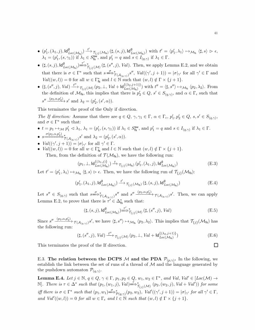
41
• (p′1, (λ1, j), Id∅Loc(Mfs)
) t′−→ T{j}(Mfs) (♯, (s, j), Id∅Loc(Mfs)
) with t′ = 〈p′1, λ1〉 7→Mfs〈♯, s〉 ⊲ ǫ,
λ1 = (p′1, (s, γ1)) if λ1 ∈ Sswfs , and p′1 = q and s ∈ I(q,γ) if λ1 ∈ Γ.
• (♯, (s, j), Id∅Loc(Mfs)
)τ ′==⇒∗
T{j}(M) (♯, (s′′, j),Val ). Then, we apply Lemma E.2, and we obtain
that there is σ ∈ Γ∗ such that sσ
==⇒∗T (A(q,γ))
s′′, Val((γ′, j + 1)) = |σ|γ′ for all γ′ ∈ Γ and
Val((w, l)) = 0 for all w ∈ Γ∗fs and l ∈ N such that (w, l) /∈ Γ× {j + 1}.
• (♯, (s′′, j),Val ) t′′−−→ T{j}(M) (p2,⊥,Val + Id{(λ2,j+1)}Loc(Mfs)
) with t′′ = 〈♯, s′′〉 7→Mfs〈p2, λ2〉. From
the definition ofMfs, this implies that there is p′2 ∈ Q, s′ ∈ S(q,γ), and α ∈ Γǫ such that
s′′(p2,α,p′2)−−−−−−→ s′ and λ2 = (p′2, (s
′, α)).
This terminates the proof of the Only if direction.
The If direction: Assume that there are q ∈ Q, γ, γ1 ∈ Γ, α ∈ Γǫ, p′1, p
′2 ∈ Q, s, s′ ∈ S(q,γ),
and σ ∈ Γ∗ such that:
• t = p1 7→M p′1 ⊳ λ1, λ1 = (p′1, (s, γ1)) if λ1 ∈ Sswfs , and p′1 = q and s ∈ I(q,γ) if λ1 ∈ Γ.
• sσ(p2,α,p′2)======⇒∗
T (A(q,γ))s′ and λ2 = (p′2, (s
′, α)).
• Val((γ′, j + 1)) = |σ|γ′ for all γ′ ∈ Γ.• Val((w, l)) = 0 for all w ∈ Γ∗
fs and l ∈ N such that (w, l) /∈ Γ× {j + 1}.
Then, from the definition of T (Mfs), we have the following run:
(p1,⊥, Id{(λ1,j)}Loc(Mfs)
) t−→ T{j}(Mfs) (p′1, (λ1, j), Id
∅Loc(Mfs)
) (E.3)
Let t′ = 〈p′1, λ1〉 7→Mfs〈♯, s〉 ⊲ ǫ. Then, we have the following run of T{j}(Mfs):
(p′1, (λ1, j), Id∅Loc(Mfs)
) t′−→ T{j}(Mfs) (♯, (s, j), Id∅Loc(Mfs)
) (E.4)
Let s′′ ∈ S(q,γ) such that sσ
==⇒∗T (A(q,γ))
s′′ and s′′(p2,α,p′2)−−−−−−→ T (A(q,γ))s
′. Then, we can apply
Lemma E.2, to prove that there is τ ′ ∈ ∆∗fs such that:
(♯, (s, j), Id∅Loc(Mfs)
)τ ′==⇒∗
T{j}(M) (♯, (s′′, j),Val ) (E.5)
Since s′′(p2,α,p′2)−−−−−−→ T (A(q,γ))s
′, we have 〈♯, s′′〉 7→Mfs〈p2, λ2〉. This implies that T{j}(Mfs) has
the following run:
(♯, (s′′, j),Val ) t′′−−→ T{j}(M) (p2,⊥,Val + Id{(λ2,j+1)}Loc(Mfs)
) (E.6)
This terminates the proof of the If direction.
E.3. The relation between the DCPS M and the PDA P(p,γ). In the following, weestablish the link between the set of runs of a thread ofM and the language generated bythe pushdown automaton P(q,γ).
Lemma E.4. Let j ∈ N, q ∈ Q, γ ∈ Γ, p1, p2 ∈ Q, w1, w2 ∈ Γ∗, and Val ,Val ′ ∈ [Loc(M)→
N]. There is τ ∈ ∆∗ such that (p1, (w1, j),Val )τ
==⇒∗T{j}(M) (p2, (w2, j),Val +Val ′)) for some
iff there is σ ∈ Γ∗ such that (p1, w1)σ
==⇒∗P(q,γ)(p2, w2), Val
′((γ′, j+1)) = |σ|γ′ for all γ′ ∈ Γ,
and Val ′((w, l)) = 0 for all w ∈ Γǫ and l ∈ N such that (w, l) /∈ Γ× {j + 1}.
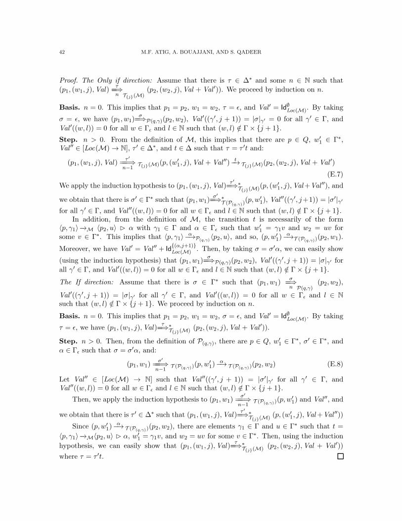
42 M.F. ATIG, A. BOUAJJANI, AND S. QADEER
Proof. The Only if direction: Assume that there is τ ∈ ∆∗ and some n ∈ N such that
(p1, (w1, j),Val )τ
==⇒n T{j}(M)
(p2, (w2, j),Val + Val ′)). We proceed by induction on n.
Basis. n = 0. This implies that p1 = p2, w1 = w2, τ = ǫ, and Val ′ = Id∅Loc(M). By taking
σ = ǫ, we have (p1, w1)σ
==⇒P(q,γ)(p2, w2), Val′((γ′, j + 1)) = |σ|γ′ = 0 for all γ′ ∈ Γ, and
Val ′((w, l)) = 0 for all w ∈ Γǫ and l ∈ N such that (w, l) /∈ Γ× {j + 1}.
Step. n > 0. From the definition of M, this implies that there are p ∈ Q, w′1 ∈ Γ∗,
Val ′′ ∈ [Loc(M)→ N], τ ′ ∈ ∆∗, and t ∈ ∆ such that τ = τ ′t and:
(p1, (w1, j),Val )τ ′
===⇒n−1
T{j}(M)(p, (w′1, j),Val + Val ′′) t−→ T{j}(M)(p2, (w2, j),Val + Val ′)
(E.7)
We apply the induction hypothesis to (p1, (w1, j),Val )τ ′==⇒∗
T{j}(M)(p, (w′1, j),Val+Val ′′), and
we obtain that there is σ′ ∈ Γ∗ such that (p1, w1)σ′
==⇒∗T (P(q,γ))
(p,w′1), Val
′′((γ′, j+1)) = |σ′|γ′
for all γ′ ∈ Γ, and Val ′′((w, l)) = 0 for all w ∈ Γǫ and l ∈ N such that (w, l) /∈ Γ× {j + 1}.In addition, from the definition of M, the transition t is necessarily of the form
〈p, γ1〉−→M 〈p2, u〉 ⊲ α with γ1 ∈ Γ and α ∈ Γǫ such that w′1 = γ1v and w2 = uv for
some v ∈ Γ∗. This implies that 〈p, γ1〉α−→P(q,γ)
〈p2, u〉, and so, (p,w′1)
α−→T (P(q,γ))(p2, w1).
Moreover, we have Val ′ = Val ′′ + Id{(α,j+1)}Loc(M) . Then, by taking σ = σ′α, we can easily show
(using the induction hypothesis) that (p1, w1)σ
==⇒P(q,γ)(p2, w2), Val′((γ′, j + 1)) = |σ|γ′ for
all γ′ ∈ Γ, and Val ′((w, l)) = 0 for all w ∈ Γǫ and l ∈ N such that (w, l) /∈ Γ× {j + 1}.
The If direction: Assume that there is σ ∈ Γ∗ such that (p1, w1)σ
==⇒n P(q,γ)
(p2, w2),
Val ′((γ′, j + 1)) = |σ|γ′ for all γ′ ∈ Γ, and Val ′((w, l)) = 0 for all w ∈ Γǫ and l ∈ N
such that (w, l) /∈ Γ× {j + 1}. We proceed by induction on n.
Basis. n = 0. This implies that p1 = p2, w1 = w2, σ = ǫ, and Val ′ = Id∅Loc(M). By taking
τ = ǫ, we have (p1, (w1, j),Val )τ
==⇒∗T{j}(M) (p2, (w2, j),Val + Val ′)).
Step. n > 0. Then, from the definition of P(q,γ), there are p ∈ Q, w′1 ∈ Γ∗, σ′ ∈ Γ∗, and
α ∈ Γǫ such that σ = σ′α, and:
(p1, w1)σ′
===⇒n−1
T (P(q,γ))(p,w′1)
α−→ T (P(q,γ))(p2, w2) (E.8)
Let Val ′′ ∈ [Loc(M) → N] such that Val ′′((γ′, j + 1)) = |σ′|γ′ for all γ′ ∈ Γ, andVal ′′((w, l)) = 0 for all w ∈ Γǫ and l ∈ N such that (w, l) /∈ Γ× {j + 1}.
Then, we apply the induction hypothesis to (p1, w1)σ′
===⇒n−1
T (P(q,γ))(p,w′1) and Val ′′, and
we obtain that there is τ ′ ∈ ∆∗ such that (p1, (w1, j),Val )τ ′==⇒∗
T{j}(M) (p, (w′1, j),Val+Val ′′))
Since (p,w′1)
α−→ T (P(q,γ))(p2, w2), there are elements γ1 ∈ Γ and u ∈ Γ∗ such that t =
〈p, γ1〉−→M〈p2, u〉 ⊲ α, w′1 = γ1v, and w2 = uv for some v ∈ Γ∗. Then, using the induction
hypothesis, we can easily show that (p1, (w1, j),Val )τ
==⇒∗T{j}(M) (p2, (w2, j),Val + Val ′))
where τ = τ ′t.
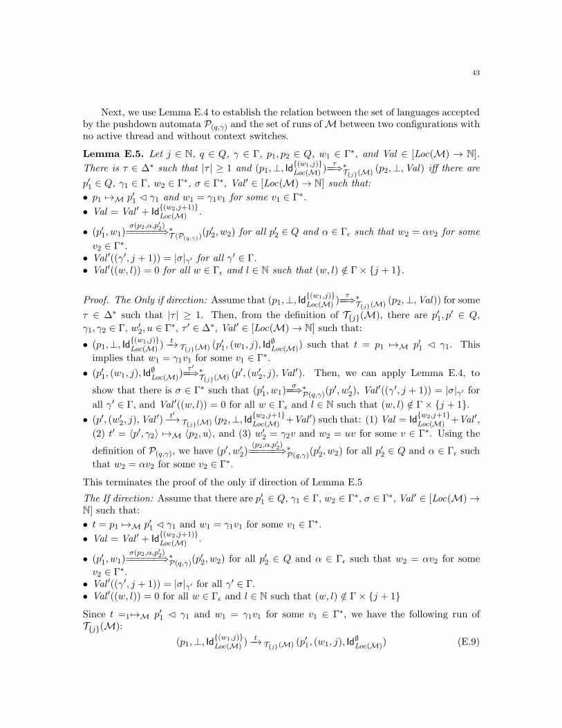
43
Next, we use Lemma E.4 to establish the relation between the set of languages acceptedby the pushdown automata P(q,γ) and the set of runs ofM between two configurations withno active thread and without context switches.
Lemma E.5. Let j ∈ N, q ∈ Q, γ ∈ Γ, p1, p2 ∈ Q, w1 ∈ Γ∗, and Val ∈ [Loc(M) → N].
There is τ ∈ ∆∗ such that |τ | ≥ 1 and (p1,⊥, Id{(w1,j)}Loc(M) )
τ==⇒∗
T{j}(M) (p2,⊥,Val) iff there are
p′1 ∈ Q, γ1 ∈ Γ, w2 ∈ Γ∗, σ ∈ Γ∗, Val ′ ∈ [Loc(M)→ N] such that:
• p1 7→M p′1 ⊳ γ1 and w1 = γ1v1 for some v1 ∈ Γ∗.
• Val = Val ′ + Id{(w2,j+1)}Loc(M) .
• (p′1, w1)σ(p2,α,p′2)======⇒∗
T (P(q,γ))(p′2, w2) for all p′2 ∈ Q and α ∈ Γǫ such that w2 = αv2 for some
v2 ∈ Γ∗.• Val ′((γ′, j + 1)) = |σ|γ′ for all γ′ ∈ Γ.• Val ′((w, l)) = 0 for all w ∈ Γǫ and l ∈ N such that (w, l) /∈ Γ× {j + 1}.
Proof. The Only if direction: Assume that (p1,⊥, Id{(w1,j)}Loc(M) )
τ==⇒∗
T{j}(M) (p2,⊥,Val)) for some
τ ∈ ∆∗ such that |τ | ≥ 1. Then, from the definition of T{j}(M), there are p′1, p′ ∈ Q,
γ1, γ2 ∈ Γ, w′2, u ∈ Γ∗, τ ′ ∈ ∆∗, Val ′ ∈ [Loc(M)→ N] such that:
• (p1,⊥, Id{(w1,j)}Loc(M) )
t−→ T{j}(M) (p′1, (w1, j), Id
∅Loc(M)) such that t = p1 7→M p′1 ⊳ γ1. This
implies that w1 = γ1v1 for some v1 ∈ Γ∗.
• (p′1, (w1, j), Id∅Loc(M))
τ ′==⇒∗
T{j}(M) (p′, (w′
2, j),Val′). Then, we can apply Lemma E.4, to
show that there is σ ∈ Γ∗ such that (p′1, w1)σ
==⇒∗P(q,γ)(p
′, w′2), Val
′((γ′, j + 1)) = |σ|γ′ for
all γ′ ∈ Γ, and Val ′((w, l)) = 0 for all w ∈ Γǫ and l ∈ N such that (w, l) /∈ Γ× {j + 1}.
• (p′, (w′2, j),Val
′) t′−→ T{j}(M) (p2,⊥, Id{w2,j+1}Loc(M) +Val ′) such that: (1) Val = Id
{w2,j+1}Loc(M) +Val ′,
(2) t′ = 〈p′, γ2〉 7→M 〈p2, u〉, and (3) w′2 = γ2v and w2 = uv for some v ∈ Γ∗. Using the
definition of P(q,γ), we have (p′, w′2)
(p2,α,p′2)======⇒∗P(q,γ)(p
′2, w2) for all p
′2 ∈ Q and α ∈ Γǫ such
that w2 = αv2 for some v2 ∈ Γ∗.
This terminates the proof of the only if direction of Lemma E.5
The If direction: Assume that there are p′1 ∈ Q, γ1 ∈ Γ, w2 ∈ Γ∗, σ ∈ Γ∗, Val ′ ∈ [Loc(M)→N] such that:
• t = p1 7→M p′1 ⊳ γ1 and w1 = γ1v1 for some v1 ∈ Γ∗.
• Val = Val ′ + Id{(w2,j+1)}Loc(M) .
• (p′1, w1)σ(p2,α,p′2)======⇒∗
P(q,γ)(p′2, w2) for all p′2 ∈ Q and α ∈ Γǫ such that w2 = αv2 for some
v2 ∈ Γ∗.• Val ′((γ′, j + 1)) = |σ|γ′ for all γ′ ∈ Γ.• Val ′((w, l)) = 0 for all w ∈ Γǫ and l ∈ N such that (w, l) /∈ Γ× {j + 1}
Since t =1 7→M p′1 ⊳ γ1 and w1 = γ1v1 for some v1 ∈ Γ∗, we have the following run ofT{j}(M):
(p1,⊥, Id{(w1,j)}Loc(M) )
t−→ T{j}(M) (p′1, (w1, j), Id
∅Loc(M)) (E.9)
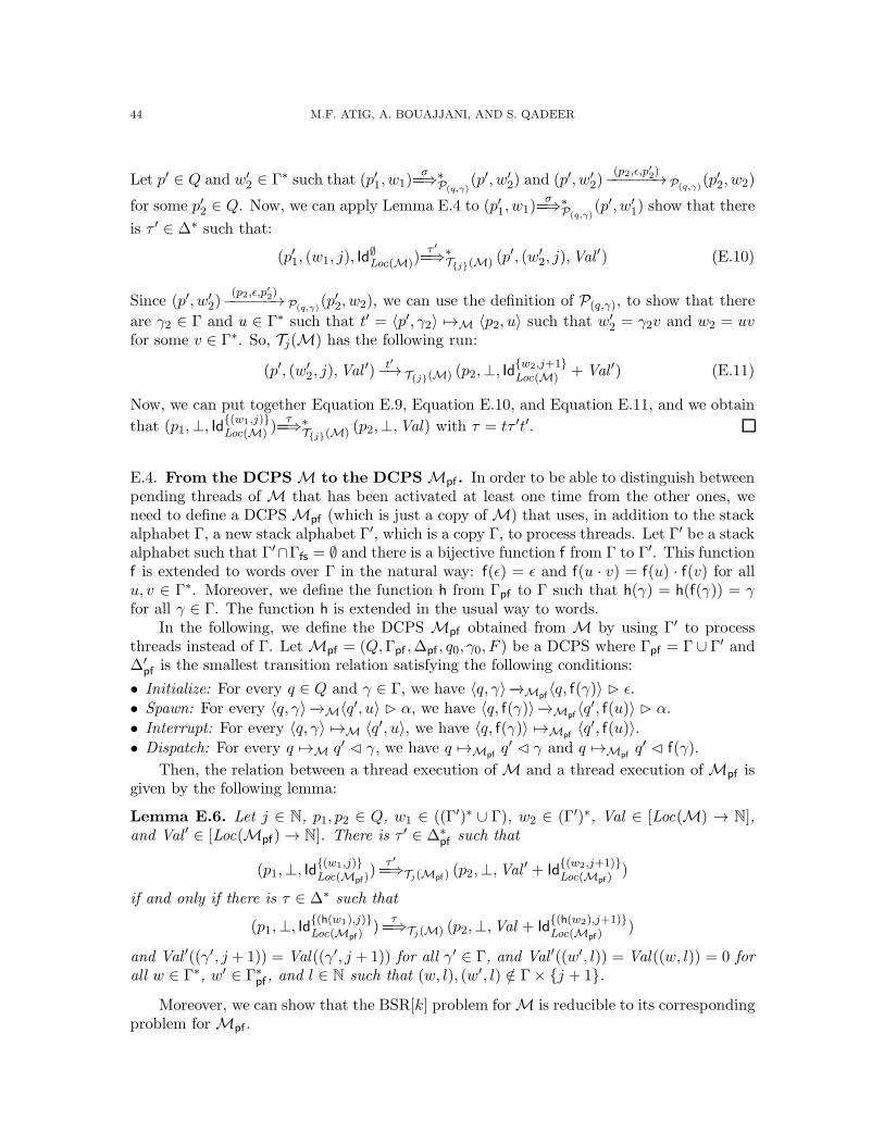
44 M.F. ATIG, A. BOUAJJANI, AND S. QADEER
Let p′ ∈ Q and w′2 ∈ Γ∗ such that (p′1, w1)
σ==⇒∗
P(q,γ)(p′, w′
2) and (p′, w′2)
(p2,ǫ,p′2)−−−−−−→ P(q,γ)(p′2, w2)
for some p′2 ∈ Q. Now, we can apply Lemma E.4 to (p′1, w1)σ
==⇒∗P(q,γ)
(p′, w′1) show that there
is τ ′ ∈ ∆∗ such that:
(p′1, (w1, j), Id∅Loc(M))
τ ′==⇒∗
T{j}(M) (p′, (w′
2, j),Val′) (E.10)
Since (p′, w′2)
(p2,ǫ,p′2)−−−−−−→ P(q,γ)(p′2, w2), we can use the definition of P(q,γ), to show that there
are γ2 ∈ Γ and u ∈ Γ∗ such that t′ = 〈p′, γ2〉 7→M 〈p2, u〉 such that w′2 = γ2v and w2 = uv
for some v ∈ Γ∗. So, Tj(M) has the following run:
(p′, (w′2, j),Val
′) t′−→ T{j}(M) (p2,⊥, Id{w2,j+1}Loc(M) + Val ′) (E.11)
Now, we can put together Equation E.9, Equation E.10, and Equation E.11, and we obtain
that (p1,⊥, Id{(w1,j)}Loc(M) )
τ==⇒∗
T{j}(M) (p2,⊥,Val) with τ = tτ ′t′.
E.4. From the DCPSM to the DCPSMpf . In order to be able to distinguish betweenpending threads of M that has been activated at least one time from the other ones, weneed to define a DCPSMpf (which is just a copy ofM) that uses, in addition to the stackalphabet Γ, a new stack alphabet Γ′, which is a copy Γ, to process threads. Let Γ′ be a stackalphabet such that Γ′∩Γfs = ∅ and there is a bijective function f from Γ to Γ′. This functionf is extended to words over Γ in the natural way: f(ǫ) = ǫ and f(u · v) = f(u) · f(v) for allu, v ∈ Γ∗. Moreover, we define the function h from Γpf to Γ such that h(γ) = h(f(γ)) = γfor all γ ∈ Γ. The function h is extended in the usual way to words.
In the following, we define the DCPS Mpf obtained from M by using Γ′ to processthreads instead of Γ. LetMpf = (Q,Γpf ,∆pf , q0, γ0, F ) be a DCPS where Γpf = Γ ∪ Γ′ and∆′
pf is the smallest transition relation satisfying the following conditions:
• Initialize: For every q ∈ Q and γ ∈ Γ, we have 〈q, γ〉−→Mpf〈q, f(γ)〉 ⊲ ǫ.
• Spawn: For every 〈q, γ〉−→M〈q′, u〉 ⊲ α, we have 〈q, f(γ)〉−→Mpf
〈q′, f(u)〉 ⊲ α.
• Interrupt: For every 〈q, γ〉 7→M 〈q′, u〉, we have 〈q, f(γ)〉 7→Mpf
〈q′, f(u)〉.• Dispatch: For every q 7→M q′ ⊳ γ, we have q 7→Mpf
q′ ⊳ γ and q 7→Mpfq′ ⊳ f(γ).
Then, the relation between a thread execution ofM and a thread execution ofMpf isgiven by the following lemma:
Lemma E.6. Let j ∈ N, p1, p2 ∈ Q, w1 ∈ ((Γ′)∗ ∪ Γ), w2 ∈ (Γ′)∗, Val ∈ [Loc(M) → N],and Val ′ ∈ [Loc(Mpf)→ N]. There is τ ′ ∈ ∆∗
pf such that
(p1,⊥, Id{(w1,j)}Loc(Mpf)
)τ ′==⇒Tj(Mpf ) (p2,⊥,Val
′ + Id{(w2,j+1)}Loc(Mpf )
)
if and only if there is τ ∈ ∆∗ such that
(p1,⊥, Id{(h(w1),j)}Loc(Mpf)
)τ
==⇒Tj(M) (p2,⊥,Val + Id{(h(w2),j+1)}Loc(Mpf )
)
and Val ′((γ′, j + 1)) = Val((γ′, j + 1)) for all γ′ ∈ Γ, and Val ′((w′, l)) = Val((w, l)) = 0 forall w ∈ Γ∗, w′ ∈ Γ∗
pf , and l ∈ N such that (w, l), (w′, l) /∈ Γ× {j + 1}.
Moreover, we can show that the BSR[k] problem forM is reducible to its correspondingproblem forMpf .
45
Lemma E.7. For every k ∈ N, a state q ∈ Q is k-bounded reachable byM if and only if qis k-bounded reachable byMpf .
E.5. From the DCPS Mpf and the DCFS Mfs to the DCPS M∪. We define theDCPS M∪ = (Q∪,Γ∪,∆∪, q0, γ0, F ) as the union of Mpf and Mfs where: (1) Q∪ = Qfs,(2) Γ∪ = Γpf ∪ Γfs is a finite set of stack symbols, and (3) ∆∪ = ∆pf ∪∆fs is the transitionrelation.
Now, we are ready to define the rank of a run of T (M∪). Intuitively, the number ofthreads that are simulated according to ∆fs (resp. ∆ls) is given by the number of pendingthreads with stack configuration in Ssw
fs × N (resp. (Γ′)∗ × N). Formally, we have:
Definition E.8. (The rank of a run of M∪) Let ρ = cinitM∪
τ==⇒∗
T[0,k](M∪)c be a run of
T[0,k](M∪) such that Active(c) = ⊥. The rank of ρ, denoted by rank (ρ), is defined by thepair (m,n) with m =
∑
(w,j)∈(Γ′)∗×NIdle(c)((w, j)) and m =
∑
(λ,j)∈Sswfs×N
Idle(c)((λ, j)).
E.6. From a run of rank (m + 1, n) of M∪ to a run of rank (m,n + 1) of M∪. Inthe following, we establish that given a run of M∪ such that there is one thread executedfollowing the set of transitions ∆pf , we can compute a run of M∪ where the execution ofthis thread is replaced by an execution of a thread following the set of transitions ∆fs. Tothis aim, we need first to prove Lemma E.9which states that for any run of a thread ofMpf ,we can construct an equivalent run of a thread ofMfs.
Lemma E.9. Let γ ∈ Γ and i, j ∈ N such that i+ j ≤ k. If there are p0, p′0, . . . , pi, p
′i ∈ Q,
w1, . . . , wi+1 ∈ (Γ′)∗, τ0, . . . , τi ∈ ∆∗∪, and Val ′0, . . . ,Val
′i ∈ [Loc(M∪)→ N] such that:
• (p0,⊥, Id{(γ,j)}Loc(M∪)
)τ0==⇒∗
T{j}(M∪)(p′0,⊥,Val
′0 + Id
{(w1,j+1)}Loc(M∪)
).
• For every l ∈ [1, i], (pl,⊥, Id{(wl,j+l)}Loc(M∪)
)τl==⇒∗
T{j+l}(M∪)(p′l,⊥,Val
′l + Id
{(wl+1,j+l+1)}Loc(M∪)
).
Then, there are λ1, . . . , λi+1 ∈ Sswfs and τ ′0, . . . , τ
′i ∈ ∆∗
∪ such that:
• (p0,⊥, Id{(γ,j)}Loc(M∪)
)τ ′0==⇒∗
T{j}(M∪)(p′0,⊥,Val
′0 + Id
{(λ1,j+1)}Loc(M∪)
).
• For every l ∈ [1, i], (pl,⊥, Id{(λl,j+l)}Loc(M∪)
)τ ′l==⇒∗
T{j+l}(M∪)(p′l,⊥,Val
′l + Id
{(λl+1,j+l+1)}Loc(M∪)
).
Proof. Let us assume there are p0, p′0, . . . , pi, p
′i ∈ Q, w1, . . . , wi+1 ∈ (Γ′)∗, τ0, . . . , τi ∈ ∆∗
∪,and Val ′0, . . . ,Val
′i ∈ [Loc(M∪)→ N] such that:
• (p0,⊥, Id{(γ,j)}Loc(M∪)
)τ0==⇒∗
T{j}(M∪)(p′0,⊥,Val
′0 + Id
{(w1,j+1)}Loc(M∪)
).
• For every l ∈ [1, i], (pl,⊥, Id{(wl,j+l)}Loc(M∪)
)τl==⇒∗
T{j+l}(M∪)(p′l,⊥,Val
′l + Id
{(wl+1,j+l+1)}Loc(M∪)
).
From now, we confuse the systemM∪ andMpf (resp. M∪ andMfs) whenM∪ behavesaccording to the set of transitions ∆pf (resp. ∆fs).
Then, we apply Lemma E.5 and Lemma E.6 to show that there are σ0, . . . , σi ∈ Γ∗,γ0, . . . , γi ∈ Γ, and g0, . . . , gi+1 ∈ Q such that:
• γ0 = γ.• For every l ∈ [0, i], pl 7→M∪ gl ⊳ γl.• σ0(p
′0, γ1, g1)σ1 · · · σi−1(p
′i−1, γi, gi)σi(p
′i, ǫ, gi+1) in L′
((g0,γ),i+1).
• For every l ∈ [0, i], Val ′l((γ′, j + l + 1)) = |σl|γ′ for all γ′ ∈ Γ.
46 M.F. ATIG, A. BOUAJJANI, AND S. QADEER
• For every l ∈ [0, i], Val ′l((w, l)) = 0 for all w ∈ Γ∗∪ and l ∈ N such that (w, l) /∈ Γ× {j +
l + 1}.
Since L′((g0,γ),i+1) ⊆ L(A(g0,γ)), there are s0, . . . , si+1 ∈ S(g0,γ) such that: (1) s0 ∈ I(g0,γ),
(2) slσl(p
′l,γl+1,gl+1)
==========⇒∗T (A(g0,γ)
)sl+1 for all l ∈ [0, i[, and (3) siσl(p
′i,ǫ,gi+1)
========⇒∗T (A(g0,γ)
)si+1.
Let λl = (gl, (sl, γl)) for all l ∈ [1, i] and λi+1 = (gi+1, (si+1, ǫ)). Since pl 7→M∪ gl ⊳ γlfor all l ∈ [1, i], we can use the definition of Mfs to show that pl 7→M∪ gl ⊳ λl for alll ∈ [1, i].
Now, we can apply Lemma E.2 to prove that there are τ ′0, . . . , τ′i ∈ ∆∗
∪ such that:
• (p0,⊥, Id{(γ,j)}Loc(M∪)
)τ ′0==⇒∗
T{j}(M∪)(p′0,⊥,Val
′0 + Id
{(λ1,j+1)}Loc(M∪)
).
• For every l ∈ [1, i], (pl,⊥, Id{(λl,j+l)}Loc(M∪)
)τ ′l==⇒∗
T{j+l}(M∪)(p′l,⊥,Val
′l + Id
{(λl+1,j+l+1)}Loc(M∪)
).
Next, we show that if some state q is k-bounded reachable by a run of M∪ of rank(m+ 1, n), then q is k-bounded reachable by a run ofM∪ of rank (m,n + 1).
Lemma E.10. Let (m,n) ∈ N × N, cinitM∪
τ==⇒∗
T[0,k](M∪)c be a run of rank (m + 1, n) such
that Active(c) = ⊥. Then, there is a run cinitM∪
τ ′==⇒∗
T[0,k](M∪)c′ of rank (m,n + 1) such that
Active(c′) = ⊥, and State(c′) = State(c).
Proof. Let us assume that cinitM∪
τ==⇒∗
T[0,k](M∪)c is a run of rank (m + 1, n) with Active(c) =
⊥. Then, by the definition of DCPSs there are i, j ∈ N, γ ∈ Γ, p0, p′0, . . . , p
′i, pi+1 ∈
Q, w1, . . . , wi+1 ∈ (Γ′)∗, κ0, τ0, κ1, τ1, . . . , τi, κi+1 ∈ ∆∗∪, and Val0,Val
′0, . . . ,Val
′i,Val i+1 ∈
[Loc(M∪)→ N] such that the following conditions are satisfied:
• i+ j ≤ k.• τ = κ0τ0κ1τ1 · · · τiκi+1.
• State(c) = pi+1 and Idle = V all + Id{(wl+1,j+l+1)}Loc(M∪)
.
• cinitM∪
κ0==⇒∗T[0,k](M∪)
(p0,⊥,Val0 + Id{(γ,j)}Loc(M∪)
).
• (p0,⊥, Id{(γ,j)}Loc(M∪)
)τ0==⇒∗
T{j}(M∪)(p′0,⊥,Val
′0 + Id
{(w1,j+1)}Loc(M∪)
).
• For every l ∈ [1, i + 1], (p′l−1,⊥,Val′l−1 + Val l−1)
κl==⇒∗T[0,k](M∪)
(pl,⊥,Val l).
• For every l ∈ [1, i], (pl,⊥, Id{(wl,j+l)}Loc(M∪)
)τl==⇒∗
T{j+l}(M∪)(p′l,⊥,Val
′l + Id
{(wl+1,j+l+1)}Loc(M∪)
).
Now, we can apply Lemma E.9 to show that there are λ1, . . . , λi+1 ∈ Sswfs as well as
τ ′0, . . . , τ′i ∈ ∆∗
∪ such that:
• (p0,⊥, Id{(γ,j)}Loc(M∪)
)τ ′0==⇒∗
T{j}(M∪)(p′0,⊥,Val
′0 + Id
{(λ1,j+1)}Loc(M∪)
).
• For every l ∈ [1, i], (pl,⊥, Id{(λl,j+l)}Loc(M∪)
)τ ′l==⇒∗
T{j+l}(M∪)(p′l,⊥,Val
′l + Id
{(λl+1,j+l+1)}Loc(M∪)
).
Then, we can use the definition of DCPSs to show that there is a run cinitM∪
τ ′==⇒∗
T[0,k](M∪)c′
of rank (m,n + 1) such that Active(c′) = ⊥ and State(c′) = State(c).
47
E.7. From a run of rank (m,n + 1) of M∪ to a run of rank (m + 1, n) of M∪. Inthe following, we establish that given a run of M∪ such that there is one thread executedfollowing the set of transitions ∆fs, we can compute a run of M∪ where the execution ofthis thread is replaced by an execution of a thread following the set of transitions ∆pf . Tothis aim, we need first to prove Lemma E.11 which states that for any run of a thread ofMfs, we can construct an equivalent run of a thread ofMpf .
Lemma E.11. Let γ ∈ Γ and i, j ∈ N such that i+ j ≤ k. If there are p0, p′0, . . . , pi, p
′i ∈ Q,
λ1, . . . , λi+1 ∈ Sswfs , τ
′0, . . . , τ
′i ∈ ∆∗
∪, and Val ′0, . . . ,Val′i ∈ [Loc(M∪)→ N] such that:
• (p0,⊥, Id{(γ,j)}Loc(M∪)
)τ ′0==⇒∗
T{j}(M∪)(p′0,⊥,Val
′0 + Id
{(λ1,j+1)}Loc(M∪)
).
• For every l ∈ [1, i], (pl,⊥, Id{(λl,j+l)}Loc(M∪)
)τ ′l==⇒∗
T{j+l}(M∪)(p′l,⊥,Val
′l + Id
{(λl+1,j+l+1)}Loc(M∪)
).
Then, there are elements w1, . . . , wi+1 ∈ (Γ′)∗, τ0, . . . , τi ∈ ∆∗∪, and Val ′′0 , . . . ,Val
′′i ∈
[Loc(M∪)→ N] such that:
• (p0,⊥, Id{(γ,j)}Loc(M∪)
)τ0==⇒∗
T{j}(M∪)(p′0,⊥,Val
′′0 + Id
{(w1,j+1)}Loc(M∪)
).
• For every l ∈ [1, i], (pl,⊥, Id{(wl,j+l)}Loc(M∪)
)τl==⇒∗
T{j+l}(M∪)(p′l,⊥,Val
′′l + Id
{(wl+1,j+l+1)}Loc(M∪)
).
• For every l ∈ [0, i], Val ′l ≤ Val ′′l .
Proof. Let us assume that there are p0, p′0, . . . , pi, p
′i ∈ Q, λ1, . . . , λi+1 ∈ Ssw
fs , τ′0, . . . , τ
′i ∈
∆∗∪, and Val ′0, . . . ,Val
′i ∈ [Loc(M∪)→ N] such that:
• (p0,⊥, Id{(γ,j)}Loc(M∪)
)τ ′0==⇒∗
T{j}(M∪)(p′0,⊥,Val
′0 + Id
{(λ1,j+1)}Loc(M∪)
).
• For every l ∈ [1, i], (pl,⊥, Id{(λl,j+l)}Loc(M∪)
)τ ′l==⇒∗
T{j+l}(M∪)(p′l,⊥,Val
′l + Id
{(λl+1,j+l+1)}Loc(M∪)
).
Then, we apply Lemma E.2 to show that there are σ0, . . . , σi ∈ Γ∗, γ0, . . . , γi ∈ Γ,α ∈ Γǫ, g0, . . . , gi+1 ∈ Q, s0 ∈ I(g0,γ), and s ∈ S(g0,γ) such that:
• γ0 = γ.• For every l ∈ [0, i], pl 7→M∪ gl ⊳ γl.• σ0(p
′0, γ1, g1)σ1 · · · σi−1(p
′i−1, γi, gi)σi(p
′i, α, gi+1) in TracesT (A(g0,γ)
)({s0}, {s}).
• For every l ∈ [0, i], Val ′l((γ′, j + l + 1)) = |σl|γ′ for all γ′ ∈ Γ.
• For every l ∈ [0, i], Val ′l((w, l)) = 0 for all w ∈ Γ∗∪ and l ∈ N such that (w, l) /∈ Γ× {j +
l + 1}.
On the other hand, we can use the Lemma E.1 to show that
σ0(p′0, γ1, g1)σ1 · · · σi−1(p
′i−1, γi, gi)σi(p
′i, ǫ, gi+1) ∈ L(A(g0,γ)).
Now, we can use the definition of L(A(g0,γ)) to show that there are σ′0, . . . , σ
′i ∈ Γ∗ such that
σ′0(p
′0, γ1, g1)σ
′1 · · · σ
′i−1(p
′i−1, γi, gi)σ
′i(p
′i, ǫ, gi+1) ∈ L′
((g0,γ),i+1) and σl � σ′l for all l ∈ [0, i].
Then, we can apply E.5 and Lemma E.6 to prove that there are w1, . . . , wi+1 ∈ (Γ′)∗,τ0, . . . , τi ∈ ∆∗
∪, and Val ′′0 , . . . ,Val′′i ∈ [Loc(M∪)→ N] such that:
• (p0,⊥, Id{(γ,j)}Loc(M∪)
)τ0==⇒∗
T{j}(M∪)(p′0,⊥,Val
′′0 + Id
{(w1,j+1)}Loc(M∪)
).
• For every l ∈ [1, i], (pl,⊥, Id{(wl,j+l)}Loc(M∪)
)τl==⇒∗
T{j+l}(M∪)(p′l,⊥,Val
′′l + Id
{(wl+1,j+l+1)}Loc(M∪)
).
• For every l ∈ [0, i], Val ′l ≤ Val ′′l .• For every l ∈ [0, i], Val ′′l ((γ
′, j + l + 1)) = |σ′l|γ′ for all γ′ ∈ Γ.
• For every l ∈ [0, i], Val ′′l ((w, l)) = 0 for all w ∈ Γ∗∪ and l ∈ N such that (w, l) /∈
Γ× {j + l + 1}.
48 M.F. ATIG, A. BOUAJJANI, AND S. QADEER
Next, we show that if some state q is k-bounded reachable by a run ofM∪ of rank (m,n+1),then q is k-bounded reachable by a run ofM∪ of rank (m+ 1, n).
Lemma E.12. Let (m,n) ∈ N × N, cinitM∪
τ==⇒∗
T[0,k](M∪)c be a run of rank (m,n + 1) such
that Active(c) = ⊥. Then, there is a run cinitM∪
τ ′==⇒∗
T[0,k](M∪)c′ of rank (m + 1, n) such that
Active(c′) = ⊥, and State(c′) = State(c).
Proof. Let us assume that cinitM∪
τ==⇒∗
T[0,k](M∪)c is a run of rank (m,n+1) such that Active(c) =
⊥. Then, we can use the definition of DCPSs and Lemma E.11 to show that there is a run
cinitM∪
τ ′==⇒∗
T[0,k](M∪)c′ of rank (m+1, n) such that Active(c′) = ⊥, and State(c′) = State(c).
This work is licensed under the Creative Commons Attribution-NoDerivs License. To viewa copy of this license, visit http://creativecommons.org/licenses/by-nd/2.0/ or send aletter to Creative Commons, 171 Second St, Suite 300, San Francisco, CA 94105, USA, orEisenacher Strasse 2, 10777 Berlin, Germany