systemic risk: from generic models to food trade networks
TRANSCRIPT

ETH Library
Systemic Risk: From GenericModels to Food Trade Networks
Doctoral Thesis
Author(s):Burkholz, Rebekka
Publication date:2016
Permanent link:https://doi.org/10.3929/ethz-a-010656937
Rights / license:In Copyright - Non-Commercial Use Permitted
This page was generated automatically upon download from the ETH Zurich Research Collection.For more information, please consult the Terms of use.
DISS. ETH Nr. 23467
Systemic Risk: From Generic Models toFood Trade Networks
A thesis submitted to attain the degree of
DOCTOR OF SCIENCES of ETH ZURICH
(Dr. sc. ETH Zurich)
presented by
REBEKKA BURKHOLZ
M.Sc. TU Darmstadt
born on 26.04.1987
citizen of Germany
accepted on the recommendation of
Prof. Dr. Dr. Frank Schweitzer
Prof. Dr. Hans J. Herrmann
Prof. Dr. James P. Gleeson
2016


Acknowledgements
Even though this thesis is about the risks associated with interdependency, I would like
to acknowledge its beauty immediately at the beginning. Many people have enriched my
life and this work would not have been possible without them. This thesis is devoted to
them.
It is my wish to express my deepest gratitude towards my advisor, Frank Schweitzer. As
a literal ‘Doktorvater’, he has guided me along the way to find my path in the scientific
world. Not only, he has built the foundation of my work. While supporting me to develop
a critical mind, he has also motivated me to ask my own research questions. I am most
grateful for his trust and support.
Also, I am very thankful towards my second advisor, Hans Herrmann. It was a pleasure
to work with him and every meeting was preparing big steps forward.
Moreover, I would like to send many thanks to James P. Gleeson. His work has been a
big source of inspiration and has formed the basis of my own. I feel honored that he has
agreed to examine this thesis.
I am most thankful for the continuous support by the ETH Risk Center and the oppor-
tunities that they have created. Special gratitude I feel towards Hans Rudolf Heinimann,
Hans Gersbach, Bastian Bergmann, and Petra Monsch. They have made the past three
years most interesting and enjoyable.
Also, I cannot express enough my gratitude towards the World Food System Center and
the people who make it the warm and open environment that I have experienced: Michelle
Grant, Bastian Flury, Amy Shreck, and Anna Katarina Gilgen. Their summer school has
significantly broadened my horizon. I owe them many thanks for the doors that they have
opened and I am most grateful for their support. Special thanks I would like to send to
Danielle Tendall, Jonas Jorin, and Johan Six for the fruitful and inspiring discussions.
Their most welcoming attitude let me enjoy every single interaction.
Further, I would like to thank Jonas Peters for his most remarkable curiosity and his kind
offer to discuss statistical challenges that I faced. I cannot thank him, Marloes Maathuis,
and Nicolai Meinshausen enough for their time and effort and the fruitful discussion. Their
course on causality has ignited in me a fire to explore the topic further.
I also owe many thanks to David Adjiashvili for all the deep discussions and the most
enjoyable collaboration. His passion for algorithms is engaging and made me look forward
to his next lecture.
At the Chair of Systems Design, I met remarkable people with whom I shared so many
moments of laughter and enlightening discussions: Adiya, Antonios, David, Emre, Gia-
como, Giona, Ingo, Mario, Matt, Nadja, Nico, Nicolas, Paraskevi, Pavlin, Rahel, Rene,

Simon, Vahan, and Yen. I feel most grateful for the time we have spent to together and
will not forget our fun at lunch and table soccer battles, or at philosophical debates. Spe-
cial thanks go to Antonios for the fruitful collaboration. Moreover, I thank Corneel for
checking my references, and Marius for the pleasant work together.
I cannot thank enough my great friends Simon, Luisa, and Tim for proof-reading parts
of my thesis and their most valuable comments and suggestions. Rene has even read the
whole thesis. I owe him my deepest gratitude. They all have supported me in various
ways, which I will always keep in good memory.
I thank all of my friends in Zurich and abroad for so many moments full of happiness that
we have shared together. Without them, my life would have been less colorful.
Furthermore, I would like to thank some special teachers whose inspiring lessons have
been invaluable for the path I took. Karsten Große-Brauckmann and Burkhard Kummerer
were so contagious in their passion for Mathematics that I can truly say, they made me
a Mathematician. Barbara Drossel fascinated me equally for complex systems and I will
always appreciate her great supervision. In Christin Schafer I found a mentor and a friend,
for whom I am most thankful. Her influence reaches far beyond the way I think about
data analysis.
There are no words to express the deep gratitude that I feel towards my family, whose
continuous support and love has carried me through the darkest and most joyful moments
in my life. And towards Rene, who has become family. He has filled my life with love and
compassion beyond the ever expected.
Contents
Contents i
Abstract vii
1 Introduction 1
1.1 Cascade processes . . . . . . . . . . . . . . . . . . . . . . . . . . . . . . . . 2
1.1.1 Generic models . . . . . . . . . . . . . . . . . . . . . . . . . . . . . 2
1.2 Systemic risk reduction . . . . . . . . . . . . . . . . . . . . . . . . . . . . . 3
1.2.1 Diversification from a systemic perspective . . . . . . . . . . . . . . 4
1.2.2 The interplay between robustness and network topology . . . . . . 5
1.3 Network uncertainty . . . . . . . . . . . . . . . . . . . . . . . . . . . . . . 5
1.4 Further relevant aspects in a systemic risk analysis . . . . . . . . . . . . . 6
1.5 International trade of staple food . . . . . . . . . . . . . . . . . . . . . . . 7
1.6 Thesis outline . . . . . . . . . . . . . . . . . . . . . . . . . . . . . . . . . . 8
I Modeling systemic risk under network uncertainty 9
2 Modeling framework 11
2.1 Introduction . . . . . . . . . . . . . . . . . . . . . . . . . . . . . . . . . . . 12
2.2 Network model . . . . . . . . . . . . . . . . . . . . . . . . . . . . . . . . . 12
2.3 Cascade model classes . . . . . . . . . . . . . . . . . . . . . . . . . . . . . 14
2.3.1 Constant Load models . . . . . . . . . . . . . . . . . . . . . . . . . 15
2.3.2 Load Redistribution models . . . . . . . . . . . . . . . . . . . . . . 18
2.3.3 Overload Redistribution models . . . . . . . . . . . . . . . . . . . . 20
i

2.4 Ensembles of initial conditions . . . . . . . . . . . . . . . . . . . . . . . . . 21
2.4.1 Notation of randomness . . . . . . . . . . . . . . . . . . . . . . . . 22
2.4.2 Random graph ensembles: A configuration model approach . . . . . 24
2.4.3 Random Thresholds . . . . . . . . . . . . . . . . . . . . . . . . . . 28
2.5 Model explorations on the macro-level via simulations . . . . . . . . . . . . 30
2.5.1 Constant Load . . . . . . . . . . . . . . . . . . . . . . . . . . . . . 31
2.5.2 Load Redistribution . . . . . . . . . . . . . . . . . . . . . . . . . . 31
2.5.3 Overload Redistribution . . . . . . . . . . . . . . . . . . . . . . . . 33
2.5.4 Discussion . . . . . . . . . . . . . . . . . . . . . . . . . . . . . . . . 35
2.6 Analytic Framework . . . . . . . . . . . . . . . . . . . . . . . . . . . . . . 35
2.6.1 Local Tree Approximation . . . . . . . . . . . . . . . . . . . . . . . 36
3 Diversification strategies in Constant Load models 41
3.1 Introduction . . . . . . . . . . . . . . . . . . . . . . . . . . . . . . . . . . . 42
3.2 Local Tree Approximation . . . . . . . . . . . . . . . . . . . . . . . . . . . 44
3.2.1 The state of the art . . . . . . . . . . . . . . . . . . . . . . . . . . . 44
3.2.2 Analytic approach for general weighted networks . . . . . . . . . . . 45
3.2.3 Specialization to ED and DD models . . . . . . . . . . . . . . . . . 50
3.3 Numerical Results . . . . . . . . . . . . . . . . . . . . . . . . . . . . . . . . 53
3.3.1 Systemic perspective . . . . . . . . . . . . . . . . . . . . . . . . . . 53
3.3.2 Mesoscopic perspective . . . . . . . . . . . . . . . . . . . . . . . . . 56
3.4 Discussion . . . . . . . . . . . . . . . . . . . . . . . . . . . . . . . . . . . . 59
4 Correlations in Constant Load models: Potential to reduce systemic risk 61
4.1 Introduction . . . . . . . . . . . . . . . . . . . . . . . . . . . . . . . . . . . 62
4.2 The threshold distribution . . . . . . . . . . . . . . . . . . . . . . . . . . . 63
4.3 Cascade results . . . . . . . . . . . . . . . . . . . . . . . . . . . . . . . . . 65
4.4 Conclusions . . . . . . . . . . . . . . . . . . . . . . . . . . . . . . . . . . . 68
5 Load redistribution in infinite random graphs 71
5.1 Introduction . . . . . . . . . . . . . . . . . . . . . . . . . . . . . . . . . . . 72
ii
5.2 Local Tree Aproximation for the LRD model:
Local Load Sharing with load Shedding . . . . . . . . . . . . . . . . . . . . 72
5.2.1 Cascade dynamics . . . . . . . . . . . . . . . . . . . . . . . . . . . 76
5.3 Results . . . . . . . . . . . . . . . . . . . . . . . . . . . . . . . . . . . . . . 77
5.4 Local Load Conservation in comparison . . . . . . . . . . . . . . . . . . . . 81
5.5 Conclusions . . . . . . . . . . . . . . . . . . . . . . . . . . . . . . . . . . . 82
6 Overload redistribution in infinite random graphs 85
6.1 Introduction . . . . . . . . . . . . . . . . . . . . . . . . . . . . . . . . . . . 86
6.2 Local Tree Approximation for the OLRD model:
Local Load Sharing with load Shedding . . . . . . . . . . . . . . . . . . . . 86
6.2.1 Discretization and iteration . . . . . . . . . . . . . . . . . . . . . . 87
6.3 Results . . . . . . . . . . . . . . . . . . . . . . . . . . . . . . . . . . . . . . 89
6.4 Conclusions . . . . . . . . . . . . . . . . . . . . . . . . . . . . . . . . . . . 91
II Extensions and limitations of modeling assumptions 93
7 Systemic risk in multiplex networks with asymmetric coupling and thresh-
old feedback 97
7.1 Introduction . . . . . . . . . . . . . . . . . . . . . . . . . . . . . . . . . . . 98
7.2 Model . . . . . . . . . . . . . . . . . . . . . . . . . . . . . . . . . . . . . . 99
7.2.1 Aggregation . . . . . . . . . . . . . . . . . . . . . . . . . . . . . . . 103
7.3 Local tree approximation . . . . . . . . . . . . . . . . . . . . . . . . . . . . 103
7.3.1 Aggregation . . . . . . . . . . . . . . . . . . . . . . . . . . . . . . . 106
7.4 Results . . . . . . . . . . . . . . . . . . . . . . . . . . . . . . . . . . . . . . 106
7.4.1 Comparison with computer simulations . . . . . . . . . . . . . . . . 106
7.4.2 Impact of the coupling strength . . . . . . . . . . . . . . . . . . . . 107
7.4.3 Scaling behavior . . . . . . . . . . . . . . . . . . . . . . . . . . . . 110
7.5 Conclusions . . . . . . . . . . . . . . . . . . . . . . . . . . . . . . . . . . . 113
8 Systemic feedback transforming constant load cascades to effective load
redistribution 116
8.1 Introduction . . . . . . . . . . . . . . . . . . . . . . . . . . . . . . . . . . . 117
iii
8.2 Local Tree Approximation incorporating systemic feedback . . . . . . . . . 117
8.3 Similarity with LRD on fully connected networks . . . . . . . . . . . . . . 119
8.4 Discussion . . . . . . . . . . . . . . . . . . . . . . . . . . . . . . . . . . . . 119
9 Cascade size distribution for finite networks 121
9.1 Introduction . . . . . . . . . . . . . . . . . . . . . . . . . . . . . . . . . . . 122
9.2 The cascade processes . . . . . . . . . . . . . . . . . . . . . . . . . . . . . 123
9.3 Cascade size distribution on fully connected networks . . . . . . . . . . . . 124
9.3.1 Model examples on fully connected networks . . . . . . . . . . . . . 125
9.4 Final cascade size distribution on star-shaped networks . . . . . . . . . . . 128
9.4.1 Model examples on star-shaped networks . . . . . . . . . . . . . . . 130
9.5 Conclusions . . . . . . . . . . . . . . . . . . . . . . . . . . . . . . . . . . . 134
III Modeling systemic risk in a data driven approach 135
10 International trade of staple food: A descriptive data analysis 141
10.1 Introduction . . . . . . . . . . . . . . . . . . . . . . . . . . . . . . . . . . . 142
10.2 The network model . . . . . . . . . . . . . . . . . . . . . . . . . . . . . . . 143
10.3 Further available information . . . . . . . . . . . . . . . . . . . . . . . . . 144
10.4 General trends . . . . . . . . . . . . . . . . . . . . . . . . . . . . . . . . . 147
10.5 International trade of maize . . . . . . . . . . . . . . . . . . . . . . . . . . 151
10.6 International trade of rice . . . . . . . . . . . . . . . . . . . . . . . . . . . 154
10.7 International trade of soybeans . . . . . . . . . . . . . . . . . . . . . . . . 156
10.8 International trade of wheat . . . . . . . . . . . . . . . . . . . . . . . . . . 158
10.9 Discussion . . . . . . . . . . . . . . . . . . . . . . . . . . . . . . . . . . . . 161
11 Overload redistribution: A dependency analysis for international trade
of staple food 167
11.1 Introduction . . . . . . . . . . . . . . . . . . . . . . . . . . . . . . . . . . . 168
11.2 A cascade model for cascading export restrictions . . . . . . . . . . . . . . 170
11.3 Measures of systemic risk . . . . . . . . . . . . . . . . . . . . . . . . . . . . 172
11.4 Shock scenarios . . . . . . . . . . . . . . . . . . . . . . . . . . . . . . . . . 173
iv

11.5 Cascade results . . . . . . . . . . . . . . . . . . . . . . . . . . . . . . . . . 176
11.5.1 Relations of interdependencies . . . . . . . . . . . . . . . . . . . . . 176
11.5.2 General trends in the evolution of systemic risk . . . . . . . . . . . 179
11.5.3 Staple characteristics . . . . . . . . . . . . . . . . . . . . . . . . . . 184
11.6 Discussion . . . . . . . . . . . . . . . . . . . . . . . . . . . . . . . . . . . . 187
12 Outlook: Towards a cascade model tailored to the international trade of
maize 191
12.1 Introduction . . . . . . . . . . . . . . . . . . . . . . . . . . . . . . . . . . . 192
12.2 Import increases as shock mitigation . . . . . . . . . . . . . . . . . . . . . 193
12.2.1 World prices . . . . . . . . . . . . . . . . . . . . . . . . . . . . . . . 194
12.2.2 Demands and exports . . . . . . . . . . . . . . . . . . . . . . . . . . 195
12.2.3 Cascade dynamics . . . . . . . . . . . . . . . . . . . . . . . . . . . 197
12.2.4 Preliminary cascade results . . . . . . . . . . . . . . . . . . . . . . 198
12.3 Trade volumes reflecting trade preferences . . . . . . . . . . . . . . . . . . 199
12.3.1 Gravitation models . . . . . . . . . . . . . . . . . . . . . . . . . . . 200
12.3.2 Modeling distortions . . . . . . . . . . . . . . . . . . . . . . . . . . 201
12.3.3 Preliminary results . . . . . . . . . . . . . . . . . . . . . . . . . . . 203
12.4 Summary and outline of possible model improvements . . . . . . . . . . . . 204
13 Summary and conclusions 207
13.1 Contributions . . . . . . . . . . . . . . . . . . . . . . . . . . . . . . . . . . 207
13.1.1 Methodological contributions . . . . . . . . . . . . . . . . . . . . . 207
13.1.2 Main insights . . . . . . . . . . . . . . . . . . . . . . . . . . . . . . 209
13.2 Future research . . . . . . . . . . . . . . . . . . . . . . . . . . . . . . . . . 215
Appendix 221
A Supplementary material to Chapter 3 221
A.1 Existence of a fixed point . . . . . . . . . . . . . . . . . . . . . . . . . . . . 221
A.2 Approximation of the convolution . . . . . . . . . . . . . . . . . . . . . . . 222
A.2.1 Convolution with the help of FFT . . . . . . . . . . . . . . . . . . . 223
v

A.3 Systemic risk for further topologies . . . . . . . . . . . . . . . . . . . . . . 224
A.4 Systemic risk for net exposures . . . . . . . . . . . . . . . . . . . . . . . . 225
B Supplementary material to Chapter 9 227
C Supplementary material to Chapter 10 229
C.1 List of countries considered in the international food trade networks . . . . 229
C.2 Data summary statistics . . . . . . . . . . . . . . . . . . . . . . . . . . . . 233
List of Figures 235
List of Tables 247
Bibliography 253
vi

Abstract
This thesis investigates the amplification of failures of dependent components in a network.
Such cascade processes are a widely observed phenomenon and are therefore studied in
diverse areas such as Physics, Finance, Epidemics, Chemistry and Electrical Engineering.
Although the cascade models are as multifaceted as the fields they belong to, they follow
similar patterns and share some common overarching principles.
This work is devoted to deepen the understanding of framework models that try to capture
these common principles. The focus lies on three generic model classes. These classes are
characterized by the load that a node distributes among its functional network neighbors
in case of its failure. For each of these model classes we quantify systemic risk by an
estimation of the cascade size evolution, i.e. the evolution of the fraction of failed nodes.
By this we complement classical risk assessments, as we study the response of the system
to a shock rather than the shock itself. Especially, we focus on cascades that start from
a small fraction of initial failures, as their devastating nature (intuitively) comes as a
surprise. Our modeling approach offers a causal explanation for such extreme events and
allows us to study the conditions in which cascades inflict a high damage.
Part I of this thesis is mainly focused on the role of heterogeneous risk diversification
strategies. We show that the common intuition that primarily failures of well connected
nodes amplify a cascade process is not always correct. Indeed, we identify situations in
which the risk of very large cascades can be reduced by the early failure of well connected
nodes. However, we note that there is no general rule that applies to all situations. Instead,
we highlight that the design and control of connected systems comes with a fundamental
system’s design question: Do we prefer systems with generally low risk of large cascades
but an increased chance of extremely large breakdowns? Or do we want to reduce the risk
of extremely large breakdowns, however coming at the expense of a generally higher risk
of large cascades? It is this question that has to be answered prior to deciding on design
concepts or control strategies for highly interconnected systems.
We obtain our results with the help of Monte Carlo simulations and analytic derivations
of ensemble averages for infinite networks that rely on locally tree-like structures. The
latter lead us to fixed point equations that we solve numerically.
In Part II, we study several extensions. These serve also as robustness check with respect
to changes in our assumptions in Part I. For instance, we study topologies that can be
decomposed into two (or more) networks that are connected in a multiplex fashion. In
this case, the cascade outcome becomes very sensitive to the connectivity between the two
networks and exhibits sharp regime shifts. This calls for caution of the oversimplification
of dependency structures. In a next step, we relax our previous restriction to infinite
networks. Precisely, we derive an analytical closed form solution for the final cascade size
vii

distribution for two special network topologies of finite size. Surprisingly, we find broad,
bi-modular, cascade size distributions. This finding questions the validity of the average
fraction of failed nodes as suitable systemic risk measure.
While following a generic modeling approach for systemic risk, we successively extend a
model in our framework to more realistic application settings. In Part III, we demonstrate
how these insights can complement the data analysis of international trade relationships.
We examine the international trade of the four major internationally traded staples: maize,
rice, soy, and wheat. With the help of a cascade process, we describe the potential re-
organization of a trade network in a given year as response to production and demand
changes. This way, we provide an economic dependency analysis that goes beyond the
identification of important trade partners and can take several risk scenarios into account.
viii

Kurzfassung auf Deutsch
Diese Dissertation untersucht die Ausbreitung des schrittweisen Versagens von Systemkom-
ponenten innerhalb eines Netzwerkes. Solche sogenannten Kaskaden sind ein weit verbre-
itetes Phanomen und werden dementsprechend in unterschiedlichen Gebieten untersucht,
zum Beispiel in der Physik, den Finanzwissenschaften, der Erforschung von Epidemien,
der Chemie und dem Elektroingeneurwesen. Auch wenn Kaskadenmodelle so facetten-
reich wie ihre Anwendungsfelder sind, weisen sie doch ahnliche Muster auf und sind in
gemeinsamen ubergreifenden Prinzipien begrundet.
Die vorliegende Arbeit ist der Vertiefung des Verstandnisses solcher Prinzipien gewidmet,
indem sie drei ubergreifende Modellklassen erforscht. Diese Klassen unterscheiden sich in
der Last, die ein Netzwerkknoten an seine Nachbarn verteilt, wenn er ausfallt. Fur jede
dieser Modellklassen quantifizieren wir das inherente systemische Risiko, indem wir die
zeitliche Entwicklung der Kaskadengrosse beschreiben, d.h. indem wir den Anteil der aus-
gefallenen Knoten berechnen. Auf diese Art und Weise erganzen wir klassische Risikobew-
ertunsansatze. Anstatt die Erschutterung eines Systems zu modellieren, sind unsere Stu-
dien auf die Reaktion des Systems auf solch eine Erschutterung fokussiert. Insbesondere
interessieren uns Kaskaden, die anfangs nur durch eine kleine Zahl an Ausfallen ausgelost
werden, da ihre Zerstorunskraft intuitiv uberraschend erscheint. Unser Modellansatz bietet
eine kausale Erklarung fur solch ungewohnliche, jedoch verheerende, Geschehen. Zudem
erlaubt er uns, eingehend die Bedingungen zu untersuchen, welche vernichtende Kaskaden
begunstigen.
Im ersten Teil dieser Arbeit konzentrieren wir uns auf die Auswirkungen heterogener
Risikodiversifikationsstrategien. Es ist eine weit verbreitete Annahme, dass vorwiegend der
Ausfall gut vernetzter Knoten zur Ausbreitung von Kaskaden fuhrt. Wir zeigen indessen
auf, dass diese Intuition nicht immer korrekt ist. In diesem Zug fuhren wir Beispiele an, in
denen das Risiko sehr grosser Kaskaden durch den fruhen Ausfall gut vernetzter Knoten
reduziert werden kann. Dennoch stellen wir fest, dass keine allgemeine Regel existiert,
die sich auf alle Situationen anwenden lasst. Stattdessen stellt sich eine fundamentale
Systemgestaltungsfrage: Bevorzugen wir Systeme, in denen das Auftreten von Kaskaden
insgesamt relativ unwahrscheinlich ist, nehmen dafur aber in Kauf, dass die Kaskaden, die
auftreten, in der Regel verheerender Natur sind? Oder mochten wir das Risiko extrem
grosser Kaskaden verringern, nehmen dafur aber hin, dass sich Kaskaden wahrscheinlich
haufiger ereignen? Diese Frage muss beantwortet werden, bevor Designkonzepte oder
Kontrollmechanismen fur hoch vernetzte Systeme entwickelt werden konnen.
Unsere Resultate gewinnen wir durch Monte Carlo Simulationen und die Herleitung an-
alytischer Ensemblemittelwerte fur unendliche Netzwerke, welche auf lokal baumartigen
Strukturen beruhen. In den analytischen Herleitungen erhalten wir Fixpunktgleichungen,
die wir numerisch losen.
ix

Im zweiten Teil der Dissertation wenden wir uns verschieden Erweiterungen des ersten
Teils zu. Diese dienen auch der Robustheitsanalyse unserer Ergebnisse hinsichtlich unserer
Annahmen im ersten Teil. Zum Beispiel betrachten wir Netzwerke, die eine Multiplex-
Struktur aufweisen, d.h., die sich in zwei (oder mehr) gekoppelte Netzwerke mit ver-
schiedenen Kantenarten zerlegen lassen. Wir beobachten in diesem Fall, dass die mittlere
Kaskadengrosse sehr sensitiv auf Aenderungen der Verbinung zwischen den beiden Netzw-
erken reagiert und plotzliche unstetige Regimeubergange aufweist. Dieses Resultat mahnt
zur Vorsicht bezuglich zu starker Vereinfachungen topologischer Netzwerkstrukturen. Im
nachsten Schritt lockern wir unsere Annahmen in Hinsicht auf die unendliche Grosse der
bisher betrachteten Netzwerke. Wir leiten eine explizite Gleichung fur die Verteilung der
finalen Kaskadengrosse im Falle zweier spezieller Netzwerkstrukturen beliebiger endlicher
Grosse her. Uberraschenderweise stellen wir fest, dass die Kaskadengrossenverteilun-
gen oftmals breite, bimodale Formen aufweisen. Diese Ergebnisse stellen die mittlere
Kaskadengrosse als valides systemisches Risikomass in Frage.
Auch wenn wir einen sehr allgemeinen Modellansatz verfolgen, passen wir eines der studierten
Modelle sukzessive an die Erfordernisse einer Anwendung an. Im dritten Teil der vorliegen-
den Arbeit erklaren wir, wie unsere gewonnenen Einsichten die Datenanalyse interna-
tionaler Handelsbeziehungen bereichern konnen. Wir erforschen den internationalen Han-
del der vier vorrangig gehandelten Grundnahrungsmittel: Mais, Reis, Soja, und Weizen.
Mithilfe eines Kaskadenprozesses beschreiben wir die mogliche Reorganisation eines Han-
delsnetzwerkes in einem gegebenen Jahr. Diese Reorganisation resultiert aus Produktions-
und Nachfrageanderungen. Damit stellen wir eine Analyse okonomischer Abhangigkeiten
zwischen Landern her, die uber die Identifikation wichtiger Handelspartner hinausgeht und
diskutieren verschiedene Risikoszenarien.
x

Chapter 1
Introduction
Cascade processes are a widely observed phenomenon. In the course of globalization
and technological advancement, systems become more interconnected and system com-
ponents more dependent on the functioning of others (Goldin and Vogel, 2010; Stiglitz,
2002). In particular for socio-economic networks (Schweitzer et al., 2009) and financial
networks (Haldane and May, 2011), we observe an increase in coupling strength and com-
plexity at the same time. Examples are global supply chains (Akkermans and Vos, 2003;
Vachon and Klassen, 2002), but also technical systems, like power grids (Brummitt et al.,
2012a; Carreras et al., 2004; Kinney et al., 2005).
The increasing connectivity in such systems has usually many advantages. For instance,
resources can be allocated where they are needed and can thus be used more efficiently.
Also, connectivity can provide redundancy and absorb local shocks. Very often, higher
connectivity is crucial for the functionality of a system. For instance, it can be necessary
to cope with increased requirements in system’s performance. Power grids might need to
serve an increased electricity demand and thus have to be expanded. More food for an
increasing world population needs to be provided and thus transported to its destination.
However, at the same time, highly connected systems are prone to cascading phenom-
ena and thus carry an eventually high amount of systemic risk. Incidents like the US
Northeast power grid blackout of 2003 (Dobson et al., 2007) or the financial crisis in
2007/2008 (Reinhart and Rogoff, 2008) have raised awareness for the downsides of in-
creasing interdependency and complexity.
Particularly in economic systems, geographically local shocks carry the potential to have
a global impact. This is of specific relevance for the international trade of staples. For
instance, farming conditions are anticipated to face strong regional changes in the course
of climate change, which in course could impact the production of staple food (Rosegrant
and Cline, 2003; Schmidhuber and Tubiello, 2007). At the same time, the increase of
world population is expected to boost demands. This situation clearly opens the way to
1
Chapter 1. Introduction
cascading effects.
1.1 Cascade processes
Whenever a complex system can be decomposed in basic similar components that depend
on or interact with each other, the failure of a few components has the potential to cause
further failures of dependent components. In this way, initial failures can get amplified
and lead to a system wide break-down. In principle, there are two basic mechanisms
that initially can lead to cascading failures. On the one hand, a component’s failure can
result from intrinsic component properties. For instance, a technical component’s age or
internal conflicts in case of social organizations can cause local failures. On the other
hand, the failure can be a consequence of an outer shock, which some components cannot
withstand (Tessone et al., 2013). The risk assessment of these (often rare) events is an
important and still demanding task in risk management (McNeil et al., 2015). Here, we
complement this perspective by focusing on cascading failures as the response of a system
to such rare events.
Continuing cascading failures are especially problematic as result of a small number of
initial failures, as their devastating outcome comes unexpected. A few component failures
are far from rare in most real-world systems. So, every system needs to be able to withstand
small shocks.
Consequently, it is a common goal in systemic risk analyses to quantify the risk of large
cascades and to analyze under which circumstances these occur. Although the models
employed in such analyses are certainly application dependent, they follow similar patterns.
With a study of generic cascade models, we contribute to a deeper understanding of these
patterns and identify relevant factors in the amplification of cascades.
1.1.1 Generic models
Examples for cascade models include models for such diverse phenomena as fiber bundles
that break under stress (Pradhan et al., 2010), epidemic spreading (Pastor-Satorras et al.,
2015), financial contagion of bank defaults (Battiston et al., 2012a; Gai and Kapadia,
2010), collective herding behavior in economic and social systems (Bikhchandani et al.,
1992; Garcia et al., 2013; Granovetter, 1978; Schweitzer and Mach, 2008; Watts, 2002), and
overload failures in power grids or other infrastructure (Motter and Lai, 2002). However,
in case of information spreading or marketing (Watts and Dodds, 2007, and references
therein), cascades usually have a positive interpretation and the goal is to maximize the
outreach of a cascade (Kempe et al., 2003). Here, we focus on negative aspects by studying
cascading failures and present several options for the reduction of systemic risk.
2
1.2. Systemic risk reduction
We specifically investigate three different cascade model classes which have been identified
by Lorenz et al. (2009). The choice of these three classes acknowledges to some extent
the fact that the intrinsic dynamics in the above outlined examples are different. At
the same time, common overarching principles are discerned that allow for a comparison.
Clearly, this requires significant simplifications of real processes. We study models that
are reduced only to the main features of cascade processes and follow this way a generic
modeling approach.
On the one side, this reduction obviously bears the risk of strong oversimplifications. On
the other side, it is impossible to model all details in a complex system. Indeed, very
often only basic mechanisms of the complex system are known. Still, in such situations
of incomplete information, decisions influencing and shaping such complex systems need
to be made. Specifically for such situations, it is important to identify similar patterns in
different cascade phenomena to train the intuition needed for decision making under high
uncertainty.
Our modeling approach comprises two main sources of simplifying assumptions:
Complex networks. Our most important simplification of a real system is introduced by
its abstraction to a network. Despite the heterogeneity of system components, we assume
that components can be associated with one type of nodes in a network and each possible
pairwise interaction or dependence corresponds to a link between two nodes. Despite their
similarity, nodes can have several features that capture their heterogeneity and characterize
their role in a cascade process.
Cascade model classes. We distinguish between three model classes: Constant Load
(CL), Load Redistribution (LRD), and Overload Redistribution (OLRD) models. In all
classes, network nodes are endowed with exactly two intrinsic variables: robustness and
fragility. The fragility corresponds to a load that a node carries, or a loss that it experiences
in the course of a cascade. If this load exceeds its robustness, a node fails and either
distributes a predefined load (CL), its whole load (LRD) or its overload (OLRD) to its
network neighbors.
Alongside the load distribution mechanism, the overall robustness and the network topol-
ogy are the main factors which determine the evolution of a cascade. The research question
how these aspects intertwine and impact systemic risk, is a repeating motif in all our in-
vestigations.
1.2 Systemic risk reduction
Every research on systemic risk is motivated by the question how we can either design
resilient systems or steer existing systems towards a state in which they are less prone to
3
Chapter 1. Introduction
the amplification of failure cascades.
A trivial answer to this question is to build isolated systems. This is because the existence
of links between nodes imply dependencies and hence introduce the possibility for cascade
propagation. Without any links, no load can be distributed and no failures amplified.
Another trivial answer is to avoid initial failures that trigger cascades. If the robustness
of all nodes in a network is high enough, the system is perfectly safe.
Both answers are usually impractical. On the one hand side, as we argued earlier, the
existence of most links is either beneficial or even essential for the functioning of a system.
Hence, building isolated systems is commonly not an option. On the other side, sufficiently
high robustness of system components is associated with high costs or might even be
impossible to achieve, such that answer two is not an option as well. Still, these two
trivial answers point towards the direction of possible measures to reduce cascade risk:
topological adjustments and increasing robustness of the system components. However,
we have to be aware that both measures can affect the system performance, as we discuss
later.
1.2.1 Diversification from a systemic perspective
Above we introduced topological adjustments as one possible measure to enhance system
resilience. Let us note that, from a node’s perspective, topological adjustments very often
influence its risk diversification. However, diversification is a two-edged sword in the
context of cascade processes. On the one hand side, well diversified nodes, i.e. nodes
which depend on many other nodes in the network, are often less exposed to the failure of
a single network neighbor. On the other hand side, well diversified nodes are usually more
vulnerable when systemic risk is high. According to classical risk management theory,
high risk diversification is beneficial for each node, as well as the system that comprises
these nodes (Allen and Gale, 2000). The rational is that high risk diversification reduces
the failure risk of each node, and thus also of their collection.
However, this view does not consider the interdependencies of such nodes and the impact
their failure has on the remaining network. Already Aristotle realized: “... the totality is
not, as it were, a mere heap, but the whole is something besides the parts ...” – the whole
is something different from merely the sum of the parts (Aristotle). Cascades result less
from properties of individual nodes, but emerge from pairwise interactions between nodes
on the micro level to systemic risk on the macro level.
Several works (Allen et al., 2011; Battiston et al., 2012a; Gai and Kapadia, 2010; Gleeson
and Cahalane, 2007; Roukny et al., 2013) have pointed out that a higher connectivity
can give rise to devastating cascades despite the high risk diversification. In these works,
the main focus is on the diversification of exposures to other nodes. In this thesis, we
4
1.3. Network uncertainty
reason that, from a systemic risk perspective, especially the diversification of damage a
node inflicts to other nodes in case of its failure, is crucial for system safety. This view
reflects the recent paradigm shift towards a more systemic perspective, where instead of
the failure risk of an individual node the system as a whole is of relevance. Consequently,
the safety of particular nodes is not necessarily aligned with the functioning of the system
anymore. For instance, a few number of highly connected nodes might face a high failure
risk, but their failure is still acceptable if it cannot spread further.
Throughout this thesis, we observe a repeating trade-off concerning system connectivity:
highly connected nodes face a significant exposure to cascades, but, at the same time,
the diversification of the damage decreases the impact their failure on the system would
have. Thus, the prevention of failures and their mitigation, i.e the prevention of the
amplification of further failures, are often alternatives rather than complements, if nodes
depend mutually on each other.
1.2.2 The interplay between robustness and network topology
As outlined, the network topology as well as the robustness of network nodes are linked to
system performance. The question remains, whether systemic risk can be reduced without
affecting this performance. In our generic models, this translates to the question, whether
we can reduce the risk of large cascades while keeping the overall distribution of robustness
among the nodes as well as the interconnectivity fixed.
We test several options to interchange the robustness of nodes in the context of random
graph ensembles. Our results pose a system design question that needs to be answered
whenever systemic risk is addressed: Which risk do we perceive as problematic? Do we
want to reduce the risk of large devastating cascades or do we want to avoid mediocre
cascades that occur frequently?
We discuss possible answers and their consequences in several contexts.
1.3 Network uncertainty
We are interested in general statements about cascade processes and the identification of
indicators for relatively high or low systemic risk. Because of this, we dedicate Part I, and
to some extent Part II, of this thesis to the study of random graph ensembles, instead of
single network instances. This means, we estimate the average systemic risk in an ensemble
comprising all networks and robustness configurations, given certain ensemble properties.
Precisely, we study an extension of the so called configuration model, in which nodes
additionally receive a random robustness. This ensemble approach is justified in situations
where rarely complete information about the precise interaction patterns between system
5
Chapter 1. Introduction
components is available, or when the networks change so quickly that the precise structure
is unknown in a particular moment in time.
Given this setting, we derive an analytic description of the average cascade size evolution
in large systems for specific models in each cascade process class. By this we provide an
important methodological extension that enables researcher to deepen their understanding
of the main influencing factors leading to the amplification of cascades.
1.4 Further relevant aspects in a systemic risk anal-
ysis
In Part II of this thesis, we discuss several extensions of our modeling approach introduced
in Part I. At the same time, we provide a critical reflection on the limitations of our previous
assumptions. In particular, we address the following three aspects.
Multiplex.The network model represents a strong simplification of a real world system.
Different types of components or agents that interact in various ways with each other are
conceptually joined as nodes and links. We study by an exemplary multiplex network how
this simplification can impact our results, as we consider two different link types instead
of only one.
From an alternative point of view, we assess systemic risk in two coupled networks, in
which cascades can propagate back and forth. We find that excluding this second network
layer would lead to a severe underestimation of systemic risk. However, especially in an
interconnected world, it is often difficult to determine the boundaries of systems.
Systemic feedback. In our cascade models, we assume that load is distributed only
locally to the nearest network neighbors. Yet, often some global information about the
system state is available and components respond to it. For instance, prices are reported in
an economic system, or a warning about a spreading disease is communicated to the pop-
ulation. Furthermore, countermeasures might be taken to prevent the further propagation
of a cascade.
Including systemic feedback, we provide with our model a further step to describe systemic
risk as system intrinsic. Such a model would not only incorporate the propagation of
cascades but also the evolution of conditions that enable them. Furthermore, it reflects
the interplay between a cascade process and the change of boundary conditions responsible
for their emergence.
Volatility of cascade sizes. In Part I, we focus on the study of the average cascade
size in infinitely large systems. However, in finite systems, this average is often not a
good representation of the actual distribution despite its frequent use. Precisely, we derive
closed form solutions for the cascade size distribution on specific network structures of
6
1.5. International trade of staple food
arbitrary finite size. We find broad and asymmetric cascade size distributions, suggesting
that the risk of large cascades is often not well represented by the average.
1.5 International trade of staple food
In Part III of this thesis, we study a real-world system that requires the consideration of
all aspects investigated in Part I and Part II.
Multiplex. We interpret the yearly international trade of the four major internationally
traded staples maize, rice, soy, and wheat as temporal weighted multiplex network. Coun-
tries are associated with network nodes. The yearly export volume from one country to
another defines the weight of a directed link between these nodes. The resulting network
is temporal, as we have information about its evolution from years 1992 to 2013. Its mul-
tiplex nature is reflected in the four different types of links, belonging to the trade of a
specific staple.
Systemic feedback. Furthermore, global information in form of prices and production
quantities is usually available to trading agents and influences their decisions. We interpret
this as probable source of systemic feedback.
Volatility of cascade sizes. The goal of our study is to assess the reorganization of the
international food trade network as response to a shock. In our case, this shock can be a
decrease in production or an increase in demand. For these shocks, several scenarios are
conceivable. On the one hand, local natural hazards, droughts, or pests can threaten the
production. On the other hand, population increase or additional alternative food usages,
e.g. biofuel production or animal feed, can increase the global demand for crops. As the
type of shock scenario and its regional proximity crucially affect the system response, we
expect a high variation in cascade outcomes.
Uncertainty. As is the case for all complex system models, we have to omit many
factors that potentially shape it. On the one hand, this is for the sake of tractability, on
the other hand, about many factors we simply lack information. In the considered case
of international trade, this includes multilateral and bilateral trade agreements, tariffs,
subsidies, and more publicly unavailable information. Clearly, these limitations impede
the thorough understanding of all mechanisms that shape the trade network. Yet, for the
purpose of systemic risk modeling, we do not need to care about all the details of the trade
network formation. Instead, we focus on distortions of already observed structures. In this
way, latent factors, unknown to us, are (ceteris paribus) preserved and remain implicitly
reflected in the network topology. Still, we have to be aware that there is a high level of
uncertainty about the precise reaction of economic actors to shocks.
While we start from a simple model of cascading export restrictions, we successively discuss
7
Chapter 1. Introduction
model improvements that take the variety of possible decisions into account.
Sources of systemic risk. Additionally to cascade risk, an interconnected system is
usually exposed to several other risks whose mitigation are a major reason for the inter-
connectivity in the first place. For instance, the participation in global trade enables the
compensation of local production shocks via imports from other parts in the world with
plentiful harvest. Also, some regions in the world are not suitable for farming of certain
staples and maintaining trade connections with other countries is a measure to compensate
for this disadvantage. Thus, a highly interdependent market and the possible emergence
of large cascades can also be interpreted as successful mitigation of local shocks. Still, the
identification of arising economic interdependencies is a relevant factor in thorough risk
analyses.
1.6 Thesis outline
The general understanding of commonalities and differences between the cascade processes
in our modeling framework is subject of Part I of this thesis. We provide an estimation of
the final cascade size under network uncertainty by means of simulations and an analytic
branching process approximation valid in large systems.
Part II is devoted to a critical reflection on our assumptions in Part I and asks to which
degree our findings are robust with respect to changes in those assumptions. For this
purpose, we study several extensions of the models presented in Part I.
In Part III, we exemplify how our insights can inspire systemic risk modeling when more
information about a system is provided by data. Precisely, our example refers to the
international trade of staple foods. Starting from our generic modeling framework, we
show how complexity can successively be added to our cascade model to describe the
reorganization of the international trade of staples as response to shocks.
8
“Il n’est pas certain que tout soit incertain. (Translation: It is not certain
that everything is uncertain.)”
Blaise Pascal, Pascal’s Pensees
Part I
Modeling systemic risk under
network uncertainty
9

Chapter 2
Modeling framework
Summary
We introduce our cascade modeling framework and explain its conceptual foun-dation. We model systems comprised of many similar but heterogeneous agentsas network and study the amplification of node failures as response to an initialshock. In extensive simulation studies, we estimate systemic risk as networkensemble average of the evolving cascade size and explore the ramificationsof our assumptions. In an overview, we highlight similarities and differencesbetween the studied model classes. In particular, we focus on the interplaybetween network interconnectivity, different risk diversification strategies ofnodes, and the distribution of their robustness. In a next step, we prepare theanalytic derivations of the studied ensemble averages to explain our findings.
Based on R. Burkholz, A. Garas, D. Langle, and F. Schweitzer, “Systemic risk from cascadingprocesses in random and scale free networks”. Working Paper. RB contributed to the design of theresearch questions. RB wrote main parts of the simulation code. RB analyzed and interpreted thesimulation results. RB wrote the text in this thesis. RB added the model and framework introductionspecifically for this thesis. Some parts are also based on R. Burkholz, A. Garas, and F. Schweitzer, “Howdamage diversification can reduce systemic risk”. Physical Review E 93, 042313.
11
Chapter 2. Modeling framework
2.1 Introduction
As outlined in the introduction of this thesis, cascade processes are a considerable source
of systemic risk in highly interconnected complex systems. Despite the differences of the
observed phenomena, they share some common overarching principles. We study models
that are reduced to such basic principles and focus on general cascade properties that are
intrinsic to a larger class of models. In this sense, we follow a generic modeling approach.
This has advantages and disadvantages.
On the one side, the simplification supports the understanding of cascade dynamics by
preventing side tracks originating in complicated model details. Moreover, it fosters com-
putational tractability. The approach is in line with the principle of parsimony, also known
as Occam’s razor (Gauch, 2003). This formulates a preference for simpler models, as they
are often better falsifiable.
On the other side, most of the time it is reasonable to assume that reality is complicated
and that many factors possibly influence the studied system. An oversimplification might
lead to wrong conclusions and diminish the value of the modeling approach. Still, we argue
that simple models serve as good starting point for successive refinement to match better
application requirements. A grounded understanding of simple models can then guide a
modeler on the way of adding complex behavior to the models. In Part III of this thesis,
we demonstrate this procedure by the example of international trade relationships.
In fact, the models in the studied framework are so flexible designed that many more
complicated models could be reduced to them by the right choice of variables. But this
reduction is often far from trivial and might not serve the modeling purpose. Still, our
theoretical investigations can assist the formulation of hypotheses and the general system
design.
The modeling of cascade processes requires certain abstractions from the real world appli-
cation that comprise essentially three elements: (1) the identification of system components
and their dependence structure, (2) the conditions under which a failure occurs, and (3)
the interaction between system components once a failure occurs.
We model the dependence structure (1) by a network, a concept that is introduced next.
The other two elements characterize the cascade processes and are described in the intro-
duction of the cascade model classes.
2.2 Network model
We associate a system’s components with nodes and their interaction or dependence pat-
terns with links in a network G = (V,E) (Newman, 2010). In the course of the thesis,
12
2.2. Network model
we interchangeably use the terms graph instead of network, vertex instead of node, and
edge instead of link as in mathematical graph theory. While V denotes the node set, E
contains links of the form (i, j) with i, j ∈ V . Such a link connects node i with node j.
Both nodes are called adjacent to each other and adjacent to the link (i, j). Moreover,
we name i and j (network) neighbors, if they are connected via a link. The number of
all neighbors of a node i is given by its degree ki. We refer to nodes with a high degree
as hubs and nodes with a low degree as leaves. This is not a precise definition, but eases
qualitative discussions. The number of nodes in the network is denoted by N := |V |.
If we call G directed, we interpret a link (i, j) as action from i towards j, for instance, the
failure of node i would impact j (but not necessarily vice versa). We refer to the number
of links that point to a node i as its in-degree kini , and to the number of links that start
in a node i as its out-degree kouti . The degree ki is the sum of its in- and out-degree:
ki = kini + kout
i .
In case that (i, j) ∈ E implies already (j, i) ∈ E, we have a mutual dependence of connected
nodes and call G undirected. Sometimes we assume that the links are additionally weighted
by weights wij ∈ EW collected in a weight set EW . The weight wij ∈ EW can indicate a
direction from node i to node j as well as the existence of a link by wij 6= 0.
1
3
5
2
4
1
3
5
2
4
1
3
5
2
4
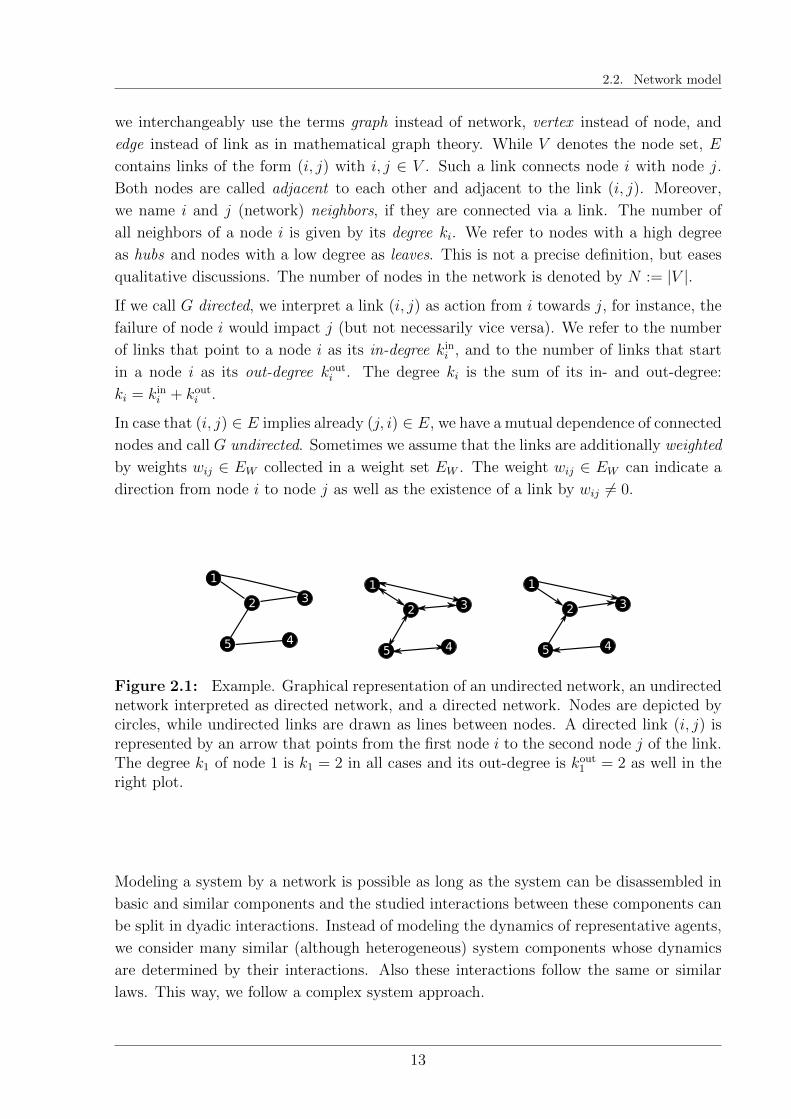
Figure 2.1: Example. Graphical representation of an undirected network, an undirectednetwork interpreted as directed network, and a directed network. Nodes are depicted bycircles, while undirected links are drawn as lines between nodes. A directed link (i, j) isrepresented by an arrow that points from the first node i to the second node j of the link.The degree k1 of node 1 is k1 = 2 in all cases and its out-degree is kout
1 = 2 as well in theright plot.
Modeling a system by a network is possible as long as the system can be disassembled in
basic and similar components and the studied interactions between these components can
be split in dyadic interactions. Instead of modeling the dynamics of representative agents,
we consider many similar (although heterogeneous) system components whose dynamics
are determined by their interactions. Also these interactions follow the same or similar
laws. This way, we follow a complex system approach.
13

Chapter 2. Modeling framework
2.3 Cascade model classes
Having abstracted from system components such as financial institutions, humans in a
society, or power stations in an electrical grid to nodes in a network, we need to formalize
what their failure means and specify how other components are affected by this.
Especially the latter can vary tremendously from system to system. A generic modeling
approach needs to account for these differences to a certain degree. Lorenz et al. (2009)
have identified three main classes of cascade processes that we generalize for the application
to weighted networks. It is a main goal of this thesis to deepen the understanding of their
commonalities and differences.
They all have in common that, on the micro-level, every node i in a network G is in one
of two states indicated by its state variable si: It is functional (si = 0) or failed (si = 1).
A possible switch of si from functional to failed is triggered either initially or in a cascade
process that evolves in discrete time steps t = 0, . . . , T . We assume in the first and second
part of this thesis that a node cannot recover. Thus, once it has failed, it stays failed
till the end T of the process. In a finite system (consisting of N nodes) a cascade ends
after T = N − 1 steps the latest, since in each time step at least one node needs to fail.
Otherwise the cascade stops. Nevertheless, it is possible that more than one node fails in
each time step.
The state si is determined by two internal node variables: the load λi that a node i carries
and the node’s threshold θi that characterizes its robustness. By Lorenz et al. (2009), the
variable λi is called fragility and is denoted by φi. Here however, we use the notation λiinstead to strengthen the association with load or loss that a node experiences. When λiexceeds the threshold θi, i.e., (λi ≥ θi), node i fails. This is equivalent to the net fragility
zi := λi − θi exceeding zero. In short, we have si(t) = H (λi(t)− θi) = H (zi(t)), where
H(·) denotes the Heaviside function. We assume that only the load λi can increase over
time, while each threshold stays constant after its initial definition, if not explicitly stated
otherwise. For simplicity, each node i receives the same initial load λi(t = 0) = λ0. Thus,
all nodes with thresholds smaller than λ0 fail in the beginning: si(0) = H (λ0 − θi). Each
failing node i distributes a total load li(t) to its remaining functional network neighbors.
It is important to note that this load li can differ from the load λi that a node carries and
needs to be defined. How the load li is distributed among the neighbors is determined
by the considered model. We consider only Markov processes, i.e., the dynamic variables
si(t+ 1), λi(t+ 1), li(t+ 1) of all nodes i = 1, · · · , N depend only on the variables at time
t. The previous history is irrelevant for the determination of t+ 1.
Let’s assume node i fails at time t and distributes the load lij(t) ∈ [0, li(t)] to its neighbor
j. We therefore have∑N
j=1 lij(t) = li(t). (lij = 0 indicates that the link does not exist or
that no load is distributed along this link.) Thus, the load λj that each neighbor carries
14
2.3. Cascade model classes
increases by lij(t). We often call lij(t) damage or impact of node i on node j. Assuming
that the loads stay at lij(t+) = lij(t) for all later times t+ > t, we can write
λj(t+ 1) =N∑i=1
lij(t)si(t) + λ0
as sum over all loads received by failing neighbors. Only nodes that have failed in the
previous time steps distribute load to a node j. Nodes that fail at the same time do not
distribute load to each other.
If a load increase causes further failures, the failing nodes distribute load again and the
cascade process keeps ongoing until no further thresholds are exceeded.
The final fraction of failed nodes, i.e. the final cascade size, serves then as our measure of
systemic risk:
%N(T ) =1
N
N∑i=1
si(T ).
If the time dependence is not explicitly stated, we denote the final cascade size by an
abbreviation (%N = %N(T )).
We compare this quantity for three main load distribution mechanisms that characterize
the load that neighbors distribute lij(t) : Constant Load (CL), Load Redistribution (LRD)
and Overload Redistribution (OLRD). In the course of their introduction, we state small
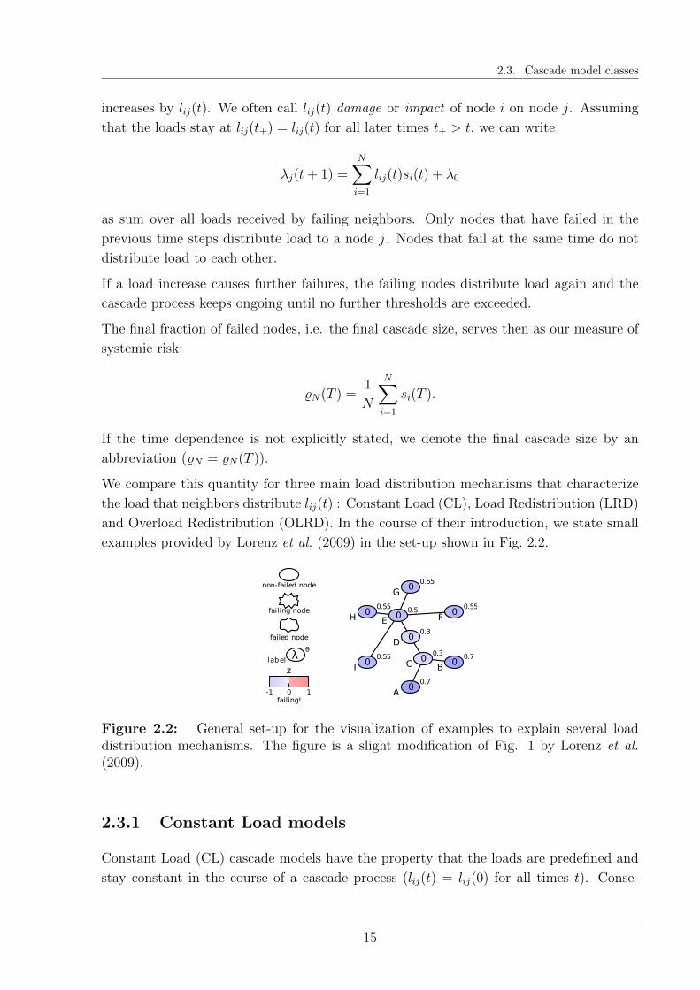
examples provided by Lorenz et al. (2009) in the set-up shown in Fig. 2.2.
label
θ
non-failed node
failing node
failed node
-1 1
z
0failing!
00.7
A
00.7
B0
0.3
C
00.3
D
00.5
E0
0.55
F
00.55
G
00.55
H
00.55
Iλ
Figure 2.2: General set-up for the visualization of examples to explain several loaddistribution mechanisms. The figure is a slight modification of Fig. 1 by Lorenz et al.(2009).
2.3.1 Constant Load models
Constant Load (CL) cascade models have the property that the loads are predefined and
stay constant in the course of a cascade process (lij(t) = lij(0) for all times t). Conse-
15
Chapter 2. Modeling framework
quently, the loads can also be associated with weights lij(t) = wij ∈ EW in a weighted
network. This simplifies the analysis in comparison to the other load redistribution classes.
Even in practice, such cascades are usually easier to control, because it is straightforward
to understand what happens next, if all information is available.
Also the time complexity is manageable, since the order of updated failures does not
influence the final cascade size. We have defined the time in which a cascade evolves
in such a way that several nodes can fail synchronously. But, in this case, it would be
sufficient to consider a random order of updated failures for estimating the final cascade
size.
Interestingly, many models for cascade estimation problems that are known to be diffi-
cult belong to the CL class. The difficulty usually originates from the high uncertainty
regarding the precise dynamics and, most importantly, the network structure. The strong
simplification is often an attempt to gain a qualitative idea what can happen (in rather
short time), while more complicated modeling approaches can hardly improve accuracy
because of the high uncertainty.
For example, the SI model in epidemic spreading (Pastor-Satorras et al., 2015) can be
mapped to our setting and belongs to the CL class. For instance, travel patterns of people
are often unknown and their form of contact unclear. In such a situation, SI-type models
prove quite useful (Brockmann and Helbing, 2013). Note that the SI-like models, despite
or because of their simplicity have been used to model various contagious processes, like
disease spreading (Pastor-Satorras and Vespignani, 2002), innovation spreading (Jackson
and Rogers, 2007), crisis spreading (Garas and Argyrakis, 2010), even herding behavior in
donations (Schweitzer and Mach, 2008). A form of opinion formation is described by the
voter model (Schweitzer and Behera, 2009) that also belongs to the CL class.
Financial contagion of bank defaults (Amini et al., 2010; Battiston et al., 2012b; Gai and
Kapadia, 2010) is another example where CL models find application. Here, contracts
between financial institutions with a certain maturity predefine (in principle) the amount
of loss that needs to be faced in case of a bank default. Still, the determination of the
weights and thresholds is far from trivial. Often the data incomplete and like the insolvency
proceedings very complicated. Often, wij would not correspond to a loss, but to a loss
relative to a node’s equity in a financial setting. For an in-depth explanation how to link
this model to a balance sheet approach, we refer the interested reader to work by Battiston
et al. (2012b) and Amini et al. (2010). Here, we just borrow the intuition for cascading
losses in a network.
We emphasize that the simplification in our framework has the consequence that we cannot
capture all models in their full complexity. For instance, many aspects of the sandpile
model (Goh et al., 2003) belong to the CL class, but we cannot describe the creation or
deletion of grains. We restrict ourselves to the study of closed systems.
16
2.3. Cascade model classes
In (Lorenz et al., 2009), two variants of CL models are proposed and called the CL Inward
and Outward variant. We study both in more detail on undirected networks, but refer to
them as Exposure and Damage Diversification models to facilitate their recognizability and
underline the purpose of our study: We explore the consequences of simple diversification
strategies on systemic risk.
The first variant, the Exposure Diversification (ED), has first been introduced by Gra-
novetter (1978) to model the formation of riots and then transferred to networks by Watts
(2002) to analyze the conditions under which global cascades can emerge, e.g., in the
spreading of rumor or opinion formation. Also the k-coreness analysis is based on this
model for a special choice of thresholds and serves, for instance, the resilience analysis of
social online communities (Garcia et al., 2013).
The load distribution weights and the load that a node carries are defined as:
w(ED)ji =
1
ki; λ
(ED)i (t+ 1) =
1
ki
N∑j=1
sj(t) =ni(t)
ki,
where w(ED)ji = 0, if there exists no link between i and j. ni(t) is defined as the number of
failed neighbors of i at time t.
Each node i is exposed to the possible total loss λi = 1, while each single neighbor’s failure
inflicts the loss 1/ki to node i. Thus, each node’s exposures are diversified and a node
experiences as loss which is precisely the fraction of its failed neighbors. The higher the
degree ki of a node, the better it is diversified. Whether a higher diversification reduces
in fact the failure risk of a node is discussed in Chap. 3.
The size of the loss that a node experiences solely depends on properties of the loss
receiving node, i.e., its degree, while the total damage that a node inflicts depends on the
neighbors’ degrees. In general, the higher the degree of a node, the higher is the damage
that its failure is expected to cause, since it affects a higher number of nodes. From a
systemic risk perspective, this effect is only problematic, if nodes with a high degree also
have a significant failure probability.
In contrast, the Damage Diversification (DD) model mitigates the potential risk amplifica-
tion by hubs, while preserving the total size of exposures∑N
i=11ki
. Instead of diversifying
a total exposure of λi = 1, the total damage lj that a node j can inflict is limited to lj = 1
and distributed equally among the network neighbors. We have:
w(DD)ji =
1
kj; λ
(ED)i (t+ 1) =
N∑j=1
1
kjsj(t),
where again w(DD)ji = 0, if there exists no link between i and j. The insight that every link
17
Chapter 2. Modeling framework
is counted once by enumerating either all starting nodes or all end nodes lets us verify that
both load distribution mechanisms, ED and DD, lead to the same total exposure Etot:
E(ED)tot =
N∑i=1
w(ED)ji =
N∑i=1
1
ki=
N∑j=1
w(DD)ji = E
(DD)tot .
In case of DD, failing hubs harm each neighbor only little, even if they affect a high
number of nodes in the network. But they usually face also a high failure risk, since every
additional neighbor means another potential loss.
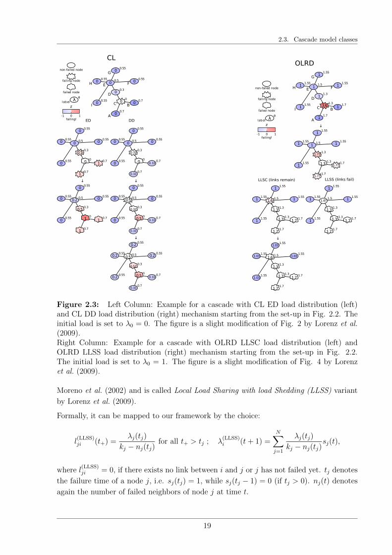
Fig. 2.3 illustrates the dynamics of both diversification variants, ED and DD, in a small
example taken from Fig. 2 in (Lorenz et al., 2009).
We explore the two models and their impact of the risk diversification strategies on sys-
temic risk in Sec. 2.5.1 via simulations and continue their analysis in Chap. 3-4 as well as
in Part II.
2.3.2 Load Redistribution models
Load Redistribution (LRD) models add complexity to the dynamics, as the load that a
node distributes is now time dependent. For this class of models, the total distributed
load li(t) coincides with the load λi(t) that a node carries itself at failure, i.e. li(t) = λi(t).
Now, the order of failures could change the outcome of the cascade evolution. We point
out again that several nodes can fail at the same time and load is only distributed to nodes
that have not failed yet. Nodes that fail at the same time, do not distribute load to each
other.
For instance, models for simplified cascades in power grids (Kinney et al., 2005) fit this
framework. Similar load distribution mechanisms can lead to cascades of forest fires
(Drossel and Schwabl, 1992) and the same models have been employed to describe earth
quakes (Jagla, 2013). One of the most prominent members of the LRD class is the fiber
bundle model (Kun et al., 2006, 2000; Pradhan et al., 2010), where a force is applied to a
bundle of fibers that is translated into a total load which is shared among the fibers. The
threshold of a fiber defines then the amount of load at which it breaks. In case of global
load sharing, a failing fiber distributes its load to all intact fibers. This corresponds, in
our setting, to a fully connected network topology. We revisit this case in Chap. 9 for
finite networks.
The local load sharing rule refers to other network topologies and the load λi(t) of a failing
node (or fiber) is only distributed to its functional network neighbors. If the network
structure itself does not change over time it can happen that load is lost. A failing node
without functional neighbors cannot distribute its load. This model has been studied by
18
2.3. Cascade model classes
label
θ
non-failed node
failing node
failed node
-1 1
z
0failing!
00.7
A
00.7
B0
0
C
00.3
D
00.5
E0
0.55
F
00.55
G
00.55
H
00.55
I
ED DD
10.7
10.70
0
0.50.3
00.5 0
0.55
00.55
00.55
00.55
↓
10.7
10.71
0
0.50.3
0.20.5 0
0.55
00.55
00.55
00.55
0.330.7
0.330.70
0
0.330.3
00.5 0
0.55
00.55
00.55
00.55
↓
0.330.7
0.330.70.5
0
0.330.3
0.50.5 0
0.55
00.55
00.55
00.55
↓
0.330.7
0.330.70.5
0
0.530.3
0.50.5 0.2
0.55
0.20.55
0.20.55
0.20.55
CL
λ
label
θ
non-failed node
failing node
failed node
-1 1
z
0failing!
11.7
A
11.7
B3.6
1.3
C
11.3
D
11.5
E1
1.55
F
11.55
G
11.55
H
11.55
I
↓
1.771.7
1.771.71.3
1.3
1.771.3
11.5 1
1.55
11.55
11.55
11.55
1.71.7
1.71.71.3
1.3
1.31.3
1.61.5 1
1.55
11.55
11.55
11.55
↓
1.71.7
1.71.71.3
1.3
1.31.3
1.61.5 1.03
1.55
1.031.55
1.031.55
1.031.55
1.71.7
1.71.71.3
1.3
1.31.3
1.471.5 1
1.55
11.55
11.55
11.55
λ
LLSC (links remain) LLSS (links fail)
OLRD
Figure 2.3: Left Column: Example for a cascade with CL ED load distribution (left)and CL DD load distribution (right) mechanism starting from the set-up in Fig. 2.2. Theinitial load is set to λ0 = 0. The figure is a slight modification of Fig. 2 by Lorenz et al.(2009).Right Column: Example for a cascade with OLRD LLSC load distribution (left) andOLRD LLSS load distribution (right) mechanism starting from the set-up in Fig. 2.2.The initial load is set to λ0 = 1. The figure is a slight modification of Fig. 4 by Lorenzet al. (2009).
Moreno et al. (2002) and is called Local Load Sharing with load Shedding (LLSS) variant
by Lorenz et al. (2009).
Formally, it can be mapped to our framework by the choice:
l(LLSS)ji (t+) =
λj(tj)
kj − nj(tj)for all t+ > tj ; λ
(LLSS)i (t+ 1) =
N∑j=1
λj(tj)
kj − nj(tj)sj(t),
where l(LLSS)ji = 0, if there exists no link between i and j or j has not failed yet. tj denotes
the failure time of a node j, i.e. sj(tj) = 1, while sj(tj − 1) = 0 (if tj > 0). nj(t) denotes
again the number of failed neighbors of node j at time t.
19

Chapter 2. Modeling framework
Apparently, the load does not need to be equally distributed among the surviving nodes.
Also general weights of the form lji(t+) = αji(t)λj(tj) with∑
i αji(t) = 1 and αji(t) ∈ [0, 1]
would fit our framework.
With the picture of fiber bundles in mind, it might be reasonable to assume that no load can
be shed, because the applied outer force is not reduced. Instead, at least the closest nodes
in the network would need to compensate for a lost fiber. Because of this, the Local Load
Sharing with load Conservation (LLSC) model variant has been investigated (Kim et al.,
2005). We relinquish its formal introduction, as we investigate it only in simulations and
we feel, the formulas would not improve the process understanding. It can be interpreted
in a way that nodes fail, but their links are still intact load is still distributed along them.
In an equivalent model formulation, the network structure changes with the evolution of
the cascade process. In case of the failure of a node, the remaining functional network
neighbors form a fully-connected clique, i.e., each functional network neighbor of the failed
node establishes a link to each other functional network neighbor of the failed node. The
load distribution follows the same law as in case of LLSS, but on the evolving network.
The model’s complexity makes it at this point impossible to study analytically. Especially
for the reason that the model has the interesting feature of increasing interconnectivity
that can enhance but also reduce systemic risk.
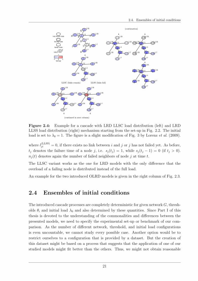
An example for the two introduced LRD models is provided by Fig. 2.4.
2.3.3 Overload Redistribution models
Overload redistribution models are similar to their LRD counterpart. The only difference
is that the overload λi(t)−θi of a failing node i is distributed instead of the full load λi(t).
Thus, failed nodes are still capable of holding a certain amount of load that equals, for
instance, their capacity.
Consequently, OLRD models are often designed to describe traffic redirection that is a
result of congestion. Examples include the Internet where the capacity of routers to
transmit information (per unit time) is exceeded (Motter, 2004; Motter and Lai, 2002) or
power-grids where the performance of power generators degrades because of an overload
(Kinney et al., 2005). Another interesting example is the Eisenberg-Noe model (Eisenberg
and Noe, 2001) which describes firms connected through a network of liabilities.
In this thesis, we focus on the LLSS and LLSC variants as for LRD models. The LLSS
weights can be similarly formulated as:
l(LLSS)ji (t+) =
λj(tj)− θjkj − nj(tj)
for all t+ > tj ; λ(LLSS)i (t+ 1) =
N∑j=1
λj(tj)− θjkj − nj(tj)
sj(t),
20
2.4. Ensembles of initial conditions
label
θ
non-failed node
failing node
failed node
-1 1
z
0failing!
11.7
A
11.7
B1
1
C
11.3
D
11.5
E1
1.55
F
11.55
G
11.55
H
11.55
I
↓
1.331.7
1.331.70
1
1.331.3
11.5 1
1.55
11.55
11.55
11.55
LLSC (links remain) LLSS (links fail)
1.671.7
1.671.70
1
01.3
1.671.5 1
1.55
11.55
11.55
11.55
↓
1.331.7
1.331.70
1
01.3
2.331.5 1
1.55
11.55
11.55
11.55
↓
(continued in next column)
(continuation)
↓
1.51.7
1.51.70
1
01.3
01.5 1.5
1.55
1.51.55
1.51.55
1.51.55
↓
1.331.7
1.331.70
1
01.3
01.5 1.58
1.55
1.581.55
1.581.55
1.581.55
↓
1.331.7
1.331.70
1
01.3
01.5 0
1.55
01.55
01.55
01.55
λ
Figure 2.4: Example for a cascade with LRD LLSC load distribution (left) and LRDLLSS load distribution (right) mechanism starting from the set-up in Fig. 2.2. The initialload is set to λ0 = 1. The figure is a slight modification of Fig. 3 by Lorenz et al. (2009).
where l(LLSS)ji = 0, if there exists no link between i and j or j has not failed yet. As before,
tj denotes the failure time of a node j, i.e. sj(tj) = 1, while sj(tj − 1) = 0 (if tj > 0).
nj(t) denotes again the number of failed neighbors of node j at time t.
The LLSC variant works as the one for LRD models with the only difference that the
overload of a failing node is distributed instead of the full load.
An example for the two introduced OLRD models is given in the right column of Fig. 2.3.
2.4 Ensembles of initial conditions
The introduced cascade processes are completely deterministic for given networkG, thresh-
olds θi and initial load λ0 and also determined by these quantities. Since Part I of this
thesis is devoted to the understanding of the commonalities and differences between the
presented models, we need to specify the experimental set-up or benchmark of our com-
parison. As the number of different network, threshold, and initial load configurations
is even uncountable, we cannot study every possible case. Another option would be to
restrict ourselves to a configuration that is provided by a dataset. But the creation of
this dataset might be based on a process that suggests that the application of one of our
studied models might fit better than the others. Thus, we might not obtain reasonable
21
Chapter 2. Modeling framework
results for the other models, as we do not test them in their ‘natural environment‘, and
the comparison would be biased. This is a pitfall that we cannot avoid completely. Nei-
ther can we ensure that our findings are generalizable to other network structures and
our interpretations might match only the specific configuration at hand. Moreover, we
cannot clearly attribute the observed effects to their cause, since too many options would
be reasonable candidates.
Because of this, we do not study single entities. Instead, we calculate the average cascade
size on an ensemble of different configurations. Evidently, the choice of this ensemble and
the probabilistic weight of an instance (i.e. the probability of their occurrence), imply a
restriction as well, and so does the focus on an average quantity. We discuss this issue
critically in Sec. 2.4.2 and Chap. 9. Also with a focus on ensembles, we cannot guarantee
that each realistic network structure for our models is represented in equal proportions
or has the same probabilistic weight. At least, we increase the probability that we also
consider situations in which an application of the studied models is reasonable.
This approach might also be justified in situations where the underlying network structure
is uncertain or changes so quickly (but on a slower time scale then the cascade process)
that it is unknown which network determines the systemic risk at a certain point in time.
Before we turn our attention to the introduction of our random graph and threshold model,
we insert a small interim section about our understanding and notation of randomness.
2.4.1 Notation of randomness
We employ basic concepts of probability theory (Feller, 1968). Thus, a probability space
(Ω,A,P) underlies most of our investigations, even though we do not mention it explicitly.
It is always assumed that the studied random variables are measurable with respect to
this probability space. We denote a random variable X : Ω → R with capital letters and
its realization by a lowercase letter x. The only exception is given by the state variable
si, s (or snb). This is always written as lowercase letter.
To indicate that a probability distribution (pdf) (or its density in case of a continuous
random variable) corresponds to a random variable X, we often denote it by pX(x) :=
P (X = x), if X is discrete. If X is a continuous random variable, pX(x) stands for its
probability density. The same applies to its cumulative distribution function for that we
reserve the capital letter F . Thus, we usually define: FX(x) = P (X ≤ x). Only in case
of the degree K of a node, we omit the subscript. We also write X ∼ pX or X ∼ FX to
indicate that X has pdf or density pX or cdf FX . If two random variables X and Y are
identically distributed, i.e., their distribution functions are identical, we also write X ∼ Y .
The conditional probability distribution P(X = x
∣∣ Y = y)
or conditional density pX|Y=y(x)
22
2.4. Ensembles of initial conditions
of X given Y are defined as usual (Feller, 1968). For P (Y = y) > 0 we can write:
P(X = x
∣∣ Y = y)
=P (X = x
⋂Y = y)
P (Y = y).
Intuitively, it expresses the probability to observe the event X = x with the knowledge
that the event Y = y has occurred already.
For instance, drawing nodes uniformly at random from a network exemplifies the concept.
Let K denote the degree of a randomly picked node and Θ its threshold. The probability
P(Θ ≤ θ
∣∣ K = k)
is the probability that a node with degree k has a threshold smaller or
equal to θ. At this point, we do not draw nodes from the whole network independently
at random. Instead we focus on all nodes with degree K = k. Thus, P(Θ ≤ θ
∣∣ K = k)
is
the probability to find nodes with a threshold of at least θ among all nodes with degree k.
We sometimes denote with X(y) a random variable with distribution P(X = x
∣∣ Y = y).
Bayes’ Theorem (here formulated for discrete random variables) follows immediately from
the concept of conditional probabilities:
P (X = x) =∑y
P(X = x
∣∣ Y = y)P (Y = y) ,
where the sum runs over all possible values of Y with nonzero probability mass, i.e.
P (Y = y) > 0. Alternatively, for continuous random variables with (Radon-Nikodym)
probability densities we have:
pX (x) =
∫pX
∣∣Y=y(x)pY (y) dy =
∫pX;Y (x, y) dy,
where pX;Y (x, y) is the joint distribution of X and Y .
Additional to the conditional probability P(X = x
∣∣ Y = y), we regard the probability
P (X = x;Y = y) = P(X = x
⋂Y = y
)that two events occur together. For instance, in our node drawing example, P (Θ ≤ θ;K = k)
is the probability to receive a node with degree k and threshold at least of the size of θ
while drawing at random from all nodes in the network.
In Part I and Part II of this thesis, we assume that the network G, the degree Ki and
threshold Θi of each node i in this network are random variables that are realized in the
beginning of a cascade process and stay constant in the course of the cascade. As these
quantities stay constant, we consider quenched and not annealed structures. Usually, the
random variables K1, · · · , Kn are assumed to be independent and identically distributed
(iid). This means, they are drawn independently at random and follow the same law (i.e.
23
Chapter 2. Modeling framework
they have the same pdf) p(·) as the one of a generic random variable K. So, we have Ki ∼ p
for all nodes i ∈ 1, · · · , N as well as K ∼ p. Also the random variables Θ1, · · · ,Θn are
not necessarily identically distributed or independent, but at least originate from an order
statistics of independent and identically distributed random variables. Usually, we assume
that the thresholds are independent, but not necessarily identically distributed.
In this setting, we calculate the fraction of failed nodes as an average with respect to the
random graph, the random degrees and the random thresholds.
2.4.2 Random graph ensembles: A configuration model approach
It is a paradigm of classical risk management theory that a higher risk diversification
reduces the failure risk of the individual, i.e. a node in a network in our case (Allen and
Gale, 2000). The question whether this paradigm holds true also with respect to systemic
risk where a higher risk diversification also increases the dependence between nodes guides
our analysis in Part I and Part II of this thesis.
With our study of a random graph ensemble, we aim at understanding the role of hetero-
geneous risk diversification strategies of nodes in a network. The diversification strategies
in the introduced models are determined by the degrees of a node. The simplest possi-
ble assumption, which does not require any further knowledge about the distribution of
random graphs, is that nodes with a prescribed diversification strategy, i.e. a prescribed
degree, connect randomly with each other without any preferences.
This describes the set-up of the configuration model that defines a random graph ensemble
where a graph is drawn uniformly at random from all possible configurations (Molloy and
Reed, 1995; Newman, 2010; Newman et al., 2001). It can be understood as entropy maxi-
mizing distribution over all graphs with the side constraint of a given degree sequence. The
model starts from such a given degree sequence k1, · · · , kN where each degree is assigned
to a node in the network that is to be constructed. These degrees can be represented as
stubs like in Fig. 2.5. Then, these stubs are paired uniformly at random so that each pair
of stubs forms a link in the constructed graph.
This procedure excludes neither the formation of multiple edges (between two nodes) nor
self-loops (that connect two stubs of the same node). We would like to avoid that a network
has these properties, because they are not the result of a reasonable risk diversification. In
finite networks, not accepting such a configuration results in a small bias, since networks
are not completely drawn uniformly at random from all possible configurations. This
problem can be overcome as proposed by Catanzaro et al. (2005). But the bias also
decreases for increasing network size N , as the probability for the occurrence of multiple
edges and self-loops converges to zero for N →∞. As our considered networks are usually
large enough (N = 105), we do not employ the more complicated algorithm. (Instead we
24
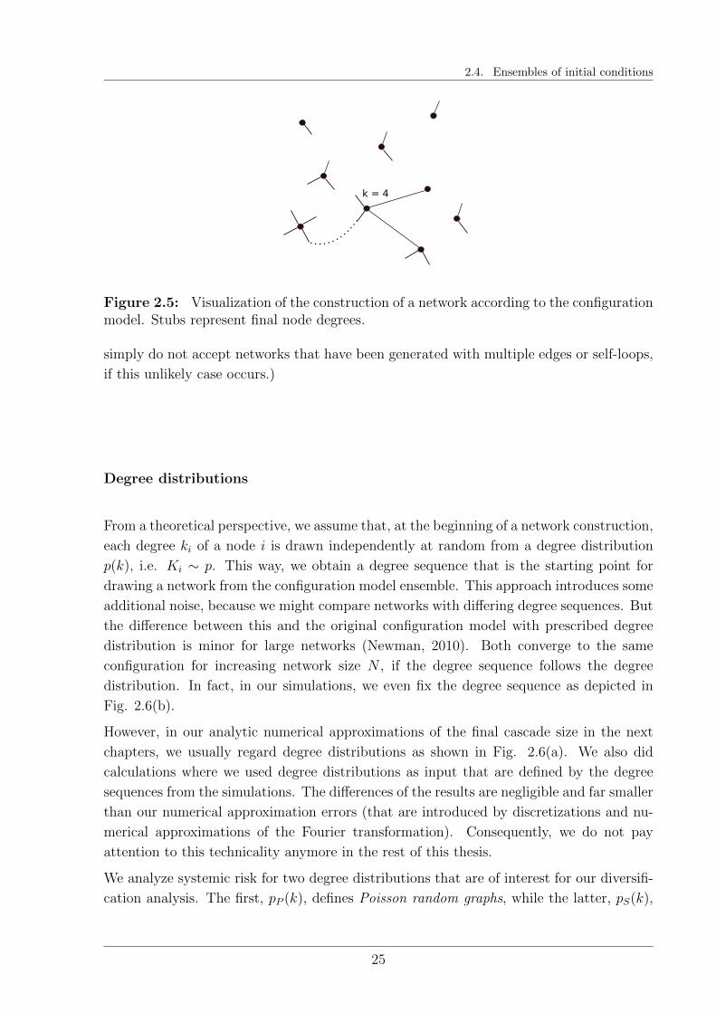
2.4. Ensembles of initial conditions
k = 4
Figure 2.5: Visualization of the construction of a network according to the configurationmodel. Stubs represent final node degrees.
simply do not accept networks that have been generated with multiple edges or self-loops,
if this unlikely case occurs.)
Degree distributions
From a theoretical perspective, we assume that, at the beginning of a network construction,
each degree ki of a node i is drawn independently at random from a degree distribution
p(k), i.e. Ki ∼ p. This way, we obtain a degree sequence that is the starting point for
drawing a network from the configuration model ensemble. This approach introduces some
additional noise, because we might compare networks with differing degree sequences. But
the difference between this and the original configuration model with prescribed degree
distribution is minor for large networks (Newman, 2010). Both converge to the same
configuration for increasing network size N , if the degree sequence follows the degree
distribution. In fact, in our simulations, we even fix the degree sequence as depicted in
Fig. 2.6(b).
However, in our analytic numerical approximations of the final cascade size in the next
chapters, we usually regard degree distributions as shown in Fig. 2.6(a). We also did
calculations where we used degree distributions as input that are defined by the degree
sequences from the simulations. The differences of the results are negligible and far smaller
than our numerical approximation errors (that are introduced by discretizations and nu-
merical approximations of the Fourier transformation). Consequently, we do not pay
attention to this technicality anymore in the rest of this thesis.
We analyze systemic risk for two degree distributions that are of interest for our diversifi-
cation analysis. The first, pP (k), defines Poisson random graphs, while the latter, pS(k),
25
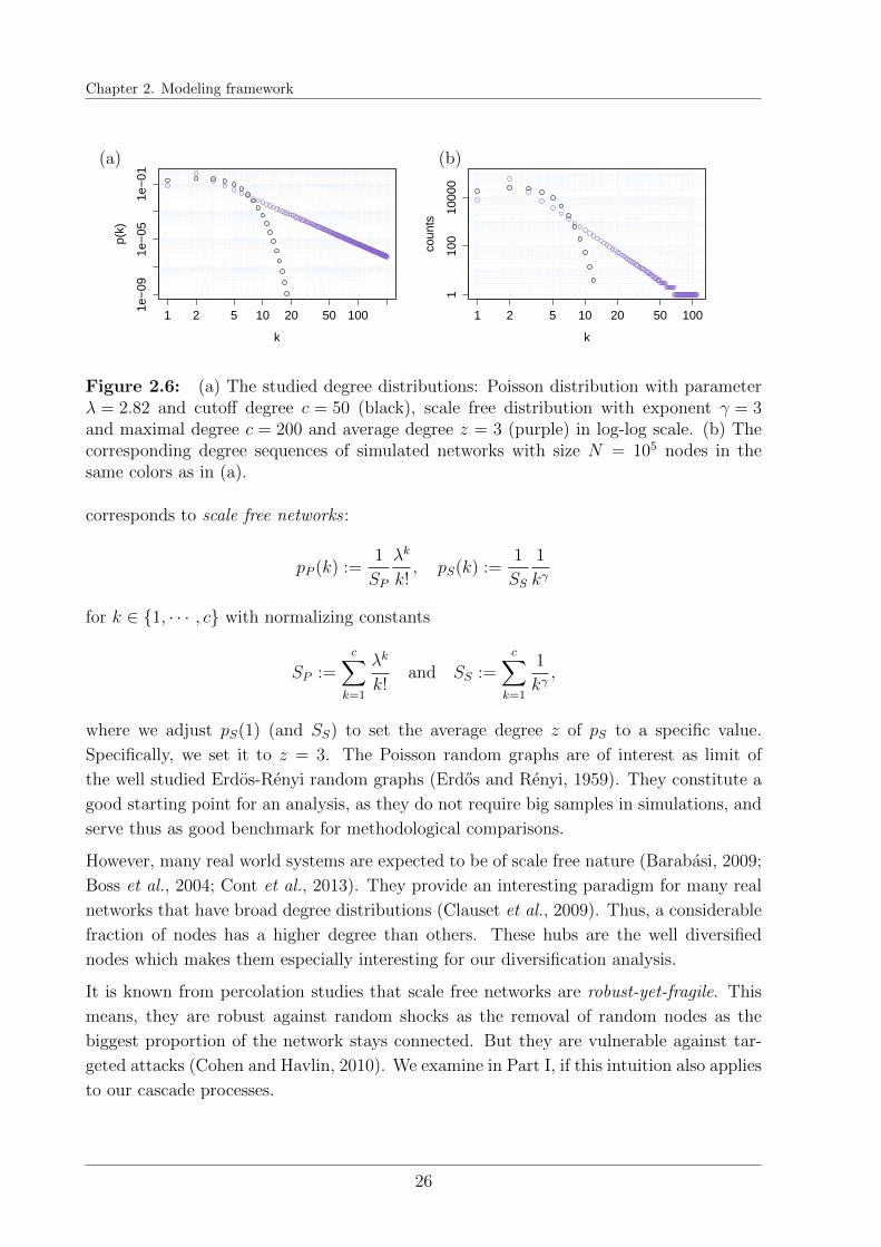
Chapter 2. Modeling framework
1 2 5 10 20 50 100
1e−
091e
−05
1e−
01
k
p(k)
1 2 5 10 20 50 100
110
010
000
k
coun
ts
(a) (b)
Figure 2.6: (a) The studied degree distributions: Poisson distribution with parameterλ = 2.82 and cutoff degree c = 50 (black), scale free distribution with exponent γ = 3and maximal degree c = 200 and average degree z = 3 (purple) in log-log scale. (b) Thecorresponding degree sequences of simulated networks with size N = 105 nodes in thesame colors as in (a).
corresponds to scale free networks :
pP (k) :=1
SP
λk
k!, pS(k) :=
1
SS
1
kγ
for k ∈ 1, · · · , c with normalizing constants
SP :=c∑
k=1
λk
k!and SS :=
c∑k=1
1
kγ,
where we adjust pS(1) (and SS) to set the average degree z of pS to a specific value.
Specifically, we set it to z = 3. The Poisson random graphs are of interest as limit of
the well studied Erdos-Renyi random graphs (Erdos and Renyi, 1959). They constitute a
good starting point for an analysis, as they do not require big samples in simulations, and
serve thus as good benchmark for methodological comparisons.
However, many real world systems are expected to be of scale free nature (Barabasi, 2009;
Boss et al., 2004; Cont et al., 2013). They provide an interesting paradigm for many real
networks that have broad degree distributions (Clauset et al., 2009). Thus, a considerable
fraction of nodes has a higher degree than others. These hubs are the well diversified
nodes which makes them especially interesting for our diversification analysis.
It is known from percolation studies that scale free networks are robust-yet-fragile. This
means, they are robust against random shocks as the removal of random nodes as the
biggest proportion of the network stays connected. But they are vulnerable against tar-
geted attacks (Cohen and Havlin, 2010). We examine in Part I, if this intuition also applies
to our cascade processes.
26

2.4. Ensembles of initial conditions
Additional to the two introduced degree distributions, we discuss regular networks where
each node has the same degree ki = z and a fully connected topology. All our models
have already been studied for fully connected networks in the limit of infinite network
size (N →∞), which is also known as thermodynamic limit in Statistical Physics (Lorenz
et al., 2009). The CL models have also been investigated on regular networks (Gleeson
and Cahalane, 2007; Lorenz et al., 2009). Meanwhile, the LRD models on regular lattices
(which are restricted to more structure than regular configuration model random graphs)
have caught the interest of several researchers (Pradhan et al., 2010; Tessone et al., 2013),
although in combination with different threshold distributions than in our study. Still, we
present them to compare heterogeneous risk diversification strategies with homogeneous
ones on regular lattices. Especially, the case of full diversification in fully connected
networks serves as benchmark in our analysis.
Please note that all degree distributions (except the fully connected one) have average
degree z = 3. Thus, we complement studies of the effect of the general connectivity on
systemic risk by an investigation of the degree heterogeneity.
Limitations of our configuration model approach
We study configuration model random graphs only for large networks. Our analytic ap-
proach is correct in the limit N →∞ and the fraction of failed nodes converges (in proba-
bility) to the calculated mean value. This indicates already that we do not consider a real
ensemble of different graphs. In fact, the topology of a large configuration model graph is
well determined and we can interchangeably talk about a fraction of nodes in the network
with a certain property or the probability that a given node has this property. We revisit
the issue of finite size effect again in Chap. 9.
The most critical assumption is thus that nodes connect without any preference, which
leads to uncorrelated networks. This means the degree Ki of a node and the degree Kj
of one of its neighbors are uncorrelated. However, most real world networks show degree-
degree correlations.
Moreover, it is an advantage and disadvantage of the configuration model that the clus-
tering coefficient converges to zero in the thermodynamic limit, if the second moment of
the degree distribution is finite, i.e.∑
k k2p(k) < ∞. This means that the probability
that two neighbors of a node are also connected to each other vanishes for N →∞. The
resulting topology is also called locally tree-like.
The analytic approach that we develop in the next chapters is based on this property. Still,
most real networks show non-zero clustering. There exist (computationally expensive)
approaches to adapt analytic approximations to this observation in clique-based random
graphs (Hackett and Gleeson, 2013).
27
Chapter 2. Modeling framework
Here, we focus on the effect of simple diversification strategies. More complexity can
always be added, if the simpler system has been well understood and higher complexity is
needed.
Extension to weighted networks
So far, we have specified an ensemble of undirected skeleton networks that defines the links
between nodes. On top of that, we can also assume random link weights Wij ≥ 0, which
might introduce a direction of the link. In general, we can have Wji 6= Wij. Considering
that a weight can also take on the value zero (wij = 0), we can construct quite flexible
directed structures. For instance, in a CL model, a node i can send a load wij to its
neighbor j but not vice versa, wji = 0, or the neighbor can send a different amount of load
wji 6= wij in case it fails before the node.
We assume that all weights Wij in the network are independent random variables. But
they do not need to be identically distributed. Instead, we allow the distributions to
depend on the degree ki of the starting node and the degree kj of the end note. Only
weights that have identical link starting node degree and identical link end node degree
are identically distributed. They follow the law of a generic random variable W (ki, kj),
i.e. Wij ∼ W (ki, kj).
2.4.3 Random Thresholds
Before the beginning of a cascade, each node i receives a degree (and network neighbors)
and then a threshold θi that is drawn independently at random from the other nodes with
the same degree. The threshold cdf can depend on the degree ki of the node and can
be represented by a random variable Θ(ki) that takes this dependence into account, i.e.
Θi ∼ FΘ(ki).
Here, we consider three cases for this dependence: (a) random failures (rf), (b) peripheral
failures (pf), and central failures (cf).
In case of random failures (a), each threshold is independent from the degree of the corre-
sponding node and drawn independently from the other thresholds. Thus, the threshold
of each node i follows the same distribution Θi ∼ FΘ.
Additionally, we consider two cases in which the threshold and the degree distribution of
the nodes are dependent. One would expect in real world situations that the robustness
and the connectivity of a node are shaped by similar mechanisms or decisions. We analyze
therefore two extreme scenarios: (b) Peripheral failures (pf) describe the case of perfect
correlation between degree and threshold distribution. Thus, nodes with a higher degree
receive a higher threshold so that nodes with smaller degrees fail initially. The opposite
28
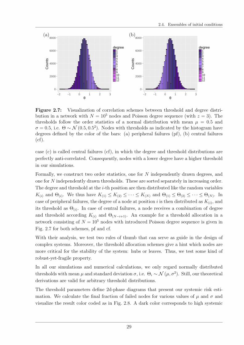
2.4. Ensembles of initial conditions
0
2000
4000
6000
8000
−2 −1 0 1 2 3θ
Cou
nts
degree123456789101112
0
2000
4000
6000
8000
−2 −1 0 1 2 3θ
Cou
nts
degree123456789101112
(a) (b)
Figure 2.7: Visualization of correlation schemes between threshold and degree distri-bution in a network with N = 105 nodes and Poisson degree sequence (with z = 3). Thethresholds follow the order statistics of a normal distribution with mean µ = 0.5 andσ = 0.5, i.e. Θ ∼ N (0.5, 0.52). Nodes with thresholds as indicated by the histogram havedegrees defined by the color of the bars: (a) peripheral failures (pf), (b) central failures(cf).
case (c) is called central failures (cf), in which the degree and threshold distributions are
perfectly anti-correlated. Consequently, nodes with a lower degree have a higher threshold
in our simulations.
Formally, we construct two order statistics, one for N independently drawn degrees, and
one for N independently drawn thresholds. These are sorted separately in increasing order.
The degree and threshold at the i-th position are then distributed like the random variables
K(i) and Θ(i). We thus have K(1) ≤ K(2) ≤ · · · ≤ K(N) and Θ(1) ≤ Θ(2) ≤ · · · ≤ Θ(N). In
case of peripheral failures, the degree of a node at position i is then distributed as K(i), and
its threshold as Θ(i). In case of central failures, a node receives a combination of degree
and threshold according K(i) and Θ(N−i+1). An example for a threshold allocation in a
network consisting of N = 105 nodes with introduced Poisson degree sequence is given in
Fig. 2.7 for both schemes, pf and cf.
With their analysis, we test two rules of thumb that can serve as guide in the design of
complex systems. Moreover, the threshold allocation schemes give a hint which nodes are
more critical for the stability of the system: hubs or leaves. Thus, we test some kind of
robust-yet-fragile property.
In all our simulations and numerical calculations, we only regard normally distributed
thresholds with mean µ and standard deviation σ, i.e. Θi ∼ N (µ, σ2). Still, our theoretical
derivations are valid for arbitrary threshold distributions.
The threshold parameters define 2d-phase diagrams that present our systemic risk esti-
mation. We calculate the final fraction of failed nodes for various values of µ and σ and
visualize the result color coded as in Fig. 2.8. A dark color corresponds to high systemic
29

Chapter 2. Modeling framework
µ
σ
0 0.2 0.4 0.6 0.8 10
0.2
0.4
0.6
0.8
1
0
0.5
1
Figure 2.8: Phase diagram for the initial fraction of failed nodes %0 = %(0) in an infinitenetwork with normally distributed thresholds (Θ ∼ N (µ, σ2)). %0 is constant along thelines σ = µ/Φ−1(%0).
risk, while the color white indicates negligible average cascade sizes. Exactly a fraction
of %(0) = FΘ (λ0) nodes fails initially in an infinitely large network, as all nodes with
initial net fragility fail in the beginning. Equivalently, a node (with unknown degree) fails
with the probability FΘ (λ0) also in a finite network. In every presented case in Part I
of this thesis, the parameters are chosen so that the initial failure probability is given by
FΘ (λ0) = Φ (−µ/σ), where Φ denotes the cdf of a standard normal distribution N (0, 1).
Consequently, %0 := %(0) is constant along the lines σ = µ/Φ−1 (0). This initial fraction
of failed nodes in infinite networks is shown in Fig. 2.8.
Similarly, we visualize the final fraction of failed nodes, our measure of systemic risk.
2.5 Model explorations on the macro-level via simu-
lations
In this section, we provide an overview of systemic risk caused by the introduced cascade
models. All phase diagrams that color code systemic risk are obtained via Monte Carlo
simulations generated with the configuration model for the Poisson and scale free degree
sequences as introduced in Sec. 2.4.2. When possible we consider networks consisting
of N = 105 nodes and generate 10 independent networks in each simulation. On each
network, we run cascades for 50 different independent threshold realizations. Thus, for
each parameter combination, we average over 500 final cascade size data points. For LRD
and OLRD LLSC models, we have to restrict our exploratory simulations to networks
consisting of N = 103 nodes, as the simulations are computationally expensive.
With this study, we transfer the analysis on fully connected networks provided by Lorenz
30
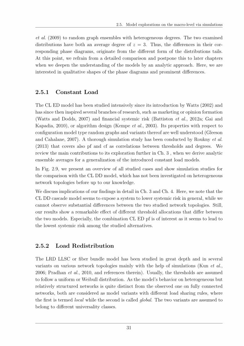
2.5. Model explorations on the macro-level via simulations
et al. (2009) to random graph ensembles with heterogeneous degrees. The two examined
distributions have both an average degree of z = 3. Thus, the differences in their cor-
responding phase diagrams, originate from the different form of the distributions tails.
At this point, we refrain from a detailed comparison and postpone this to later chapters
when we deepen the understanding of the models by an analytic approach. Here, we are
interested in qualitative shapes of the phase diagrams and prominent differences.
2.5.1 Constant Load
The CL ED model has been studied intensively since its introduction by Watts (2002) and
has since then inspired several branches of research, such as marketing or opinion formation
(Watts and Dodds, 2007) and financial systemic risk (Battiston et al., 2012a; Gai and
Kapadia, 2010), or algorithm design (Kempe et al., 2003). Its properties with respect to
configuration model type random graphs and variants thereof are well understood (Gleeson
and Cahalane, 2007). A thorough simulation study has been conducted by Roukny et al.
(2013) that covers also pf and cf as correlations between thresholds and degrees. We
review the main contributions to its exploration further in Ch. 3 , when we derive analytic
ensemble averages for a generalization of the introduced constant load models.
In Fig. 2.9, we present an overview of all studied cases and show simulation studies for
the comparison with the CL DD model, which has not been investigated on heterogeneous
network topologies before up to our knowledge.
We discuss implications of our findings in detail in Ch. 3 and Ch. 4. Here, we note that the
CL DD cascade model seems to expose a system to lower systemic risk in general, while we
cannot observe substantial differences between the two studied network topologies. Still,
our results show a remarkable effect of different threshold allocations that differ between
the two models. Especially, the combination CL ED pf is of interest as it seems to lead to
the lowest systemic risk among the studied alternatives.
2.5.2 Load Redistribution
The LRD LLSC or fiber bundle model has been studied in great depth and in several
variants on various network topologies mainly with the help of simulations (Kun et al.,
2006; Pradhan et al., 2010, and references therein). Usually, the thresholds are assumed
to follow a uniform or Weibull distribution. As the model’s behavior on heterogeneous but
relatively structured networks is quite distinct from the observed one on fully connected
networks, both are considered as model variants with different load sharing rules, where
the first is termed local while the second is called global. The two variants are assumed to
belong to different universality classes.
31
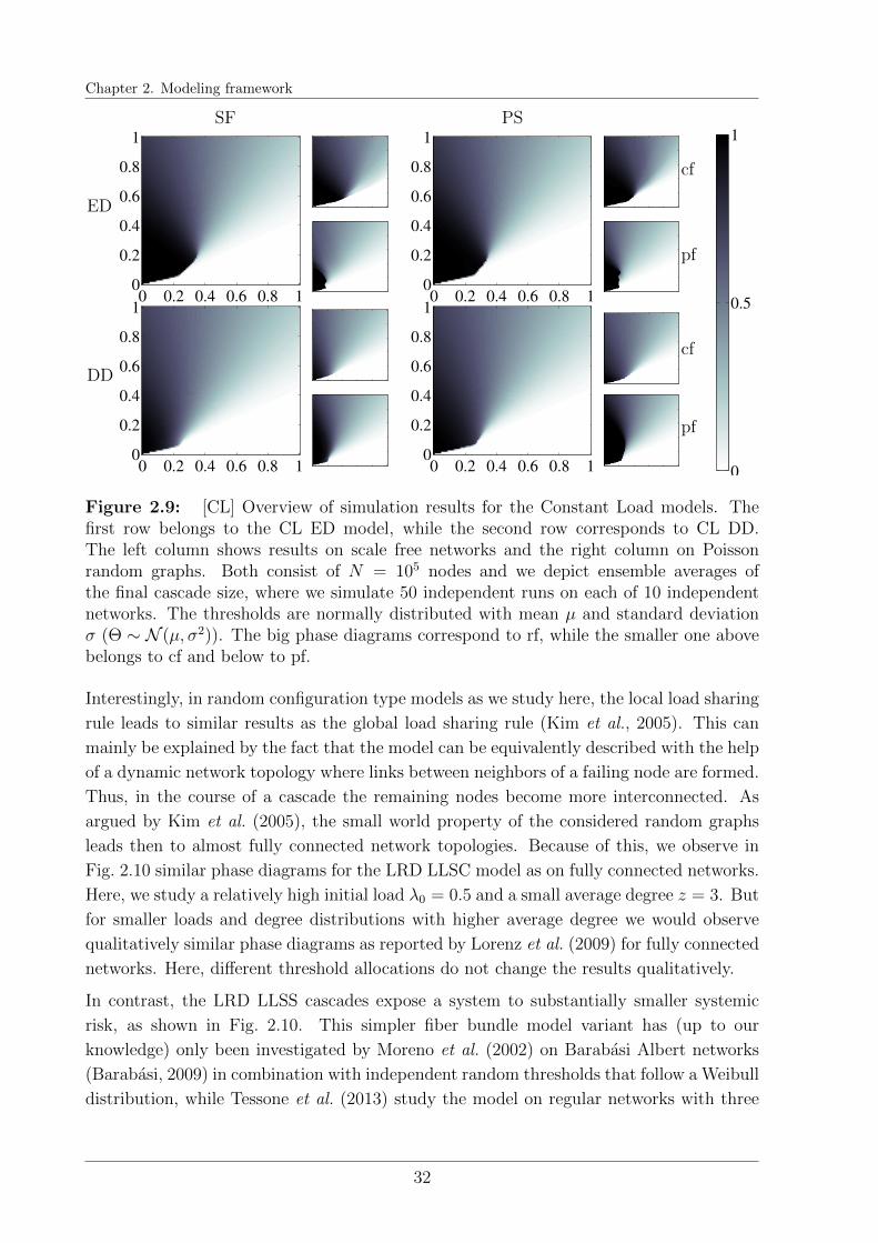
Chapter 2. Modeling framework
0 0.2 0.4 0.6 0.8 10
0.2
0.4
0.6
0.8
1
0 0.2 0.4 0.6 0.8 10
0.2
0.4
0.6
0.8
10 0.2 0.4 0.6 0.8 10
0.2
0.4
0.6
0.8
1
0 0.2 0.4 0.6 0.8 10
0.2
0.4
0.6
0.8
1
0
0.5
1
SF PS
ED
DD
cf
pf
cf
pf
Figure 2.9: [CL] Overview of simulation results for the Constant Load models. Thefirst row belongs to the CL ED model, while the second row corresponds to CL DD.The left column shows results on scale free networks and the right column on Poissonrandom graphs. Both consist of N = 105 nodes and we depict ensemble averages ofthe final cascade size, where we simulate 50 independent runs on each of 10 independentnetworks. The thresholds are normally distributed with mean µ and standard deviationσ (Θ ∼ N (µ, σ2)). The big phase diagrams correspond to rf, while the smaller one abovebelongs to cf and below to pf.
Interestingly, in random configuration type models as we study here, the local load sharing
rule leads to similar results as the global load sharing rule (Kim et al., 2005). This can
mainly be explained by the fact that the model can be equivalently described with the help
of a dynamic network topology where links between neighbors of a failing node are formed.
Thus, in the course of a cascade the remaining nodes become more interconnected. As
argued by Kim et al. (2005), the small world property of the considered random graphs
leads then to almost fully connected network topologies. Because of this, we observe in
Fig. 2.10 similar phase diagrams for the LRD LLSC model as on fully connected networks.
Here, we study a relatively high initial load λ0 = 0.5 and a small average degree z = 3. But
for smaller loads and degree distributions with higher average degree we would observe
qualitatively similar phase diagrams as reported by Lorenz et al. (2009) for fully connected
networks. Here, different threshold allocations do not change the results qualitatively.
In contrast, the LRD LLSS cascades expose a system to substantially smaller systemic
risk, as shown in Fig. 2.10. This simpler fiber bundle model variant has (up to our
knowledge) only been investigated by Moreno et al. (2002) on Barabasi Albert networks
(Barabasi, 2009) in combination with independent random thresholds that follow a Weibull
distribution, while Tessone et al. (2013) study the model on regular networks with three
32
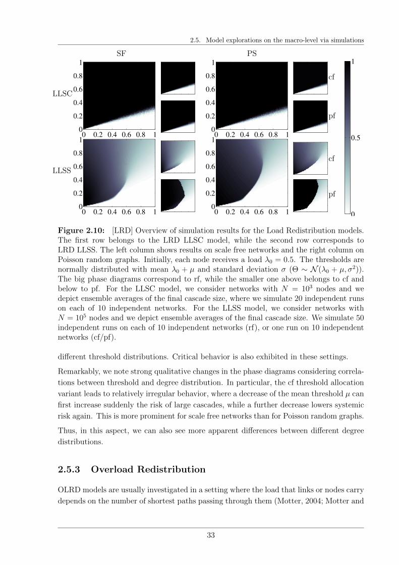
2.5. Model explorations on the macro-level via simulations
0 0.2 0.4 0.6 0.8 10
0.2
0.4
0.6
0.8
1
0 0.2 0.4 0.6 0.8 10
0.2
0.4
0.6
0.8
10 0.2 0.4 0.6 0.8 10
0.2
0.4
0.6
0.8
1
0 0.2 0.4 0.6 0.8 10
0.2
0.4
0.6
0.8
1
0
0.5
1
SF PS
LLSC
LLSS
cf
pf
cf
pf
Figure 2.10: [LRD] Overview of simulation results for the Load Redistribution models.The first row belongs to the LRD LLSC model, while the second row corresponds toLRD LLSS. The left column shows results on scale free networks and the right column onPoisson random graphs. Initially, each node receives a load λ0 = 0.5. The thresholds arenormally distributed with mean λ0 + µ and standard deviation σ (Θ ∼ N (λ0 + µ, σ2)).The big phase diagrams correspond to rf, while the smaller one above belongs to cf andbelow to pf. For the LLSC model, we consider networks with N = 103 nodes and wedepict ensemble averages of the final cascade size, where we simulate 20 independent runson each of 10 independent networks. For the LLSS model, we consider networks withN = 105 nodes and we depict ensemble averages of the final cascade size. We simulate 50independent runs on each of 10 independent networks (rf), or one run on 10 independentnetworks (cf/pf).
different threshold distributions. Critical behavior is also exhibited in these settings.
Remarkably, we note strong qualitative changes in the phase diagrams considering correla-
tions between threshold and degree distribution. In particular, the cf threshold allocation
variant leads to relatively irregular behavior, where a decrease of the mean threshold µ can
first increase suddenly the risk of large cascades, while a further decrease lowers systemic
risk again. This is more prominent for scale free networks than for Poisson random graphs.
Thus, in this aspect, we can also see more apparent differences between different degree
distributions.
2.5.3 Overload Redistribution
OLRD models are usually investigated in a setting where the load that links or nodes carry
depends on the number of shortest paths passing through them (Motter, 2004; Motter and
33
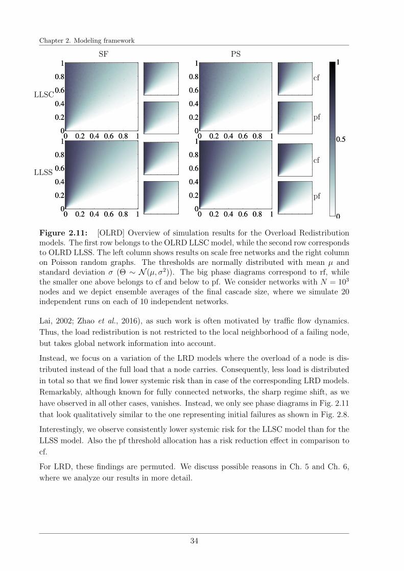
Chapter 2. Modeling framework
0 0.2 0.4 0.6 0.8 10
0.2
0.4
0.6
0.8
1
0 0.2 0.4 0.6 0.8 10
0.2
0.4
0.6
0.8
10 0.2 0.4 0.6 0.8 10
0.2
0.4
0.6
0.8
1
0 0.2 0.4 0.6 0.8 10
0.2
0.4
0.6
0.8
1
0
0.5
1
0 0.2 0.4 0.6 0.8 10
0.2
0.4
0.6
0.8
1
0 0.2 0.4 0.6 0.8 10
0.2
0.4
0.6
0.8
10 0.2 0.4 0.6 0.8 10
0.2
0.4
0.6
0.8
1
0 0.2 0.4 0.6 0.8 10
0.2
0.4
0.6
0.8
1
0
0.5
1
SF PS
LLSC
LLSS
cf
pf
cf
pf
Figure 2.11: [OLRD] Overview of simulation results for the Overload Redistributionmodels. The first row belongs to the OLRD LLSC model, while the second row correspondsto OLRD LLSS. The left column shows results on scale free networks and the right columnon Poisson random graphs. The thresholds are normally distributed with mean µ andstandard deviation σ (Θ ∼ N (µ, σ2)). The big phase diagrams correspond to rf, whilethe smaller one above belongs to cf and below to pf. We consider networks with N = 103
nodes and we depict ensemble averages of the final cascade size, where we simulate 20independent runs on each of 10 independent networks.
Lai, 2002; Zhao et al., 2016), as such work is often motivated by traffic flow dynamics.
Thus, the load redistribution is not restricted to the local neighborhood of a failing node,
but takes global network information into account.
Instead, we focus on a variation of the LRD models where the overload of a node is dis-
tributed instead of the full load that a node carries. Consequently, less load is distributed
in total so that we find lower systemic risk than in case of the corresponding LRD models.
Remarkably, although known for fully connected networks, the sharp regime shift, as we
have observed in all other cases, vanishes. Instead, we only see phase diagrams in Fig. 2.11
that look qualitatively similar to the one representing initial failures as shown in Fig. 2.8.
Interestingly, we observe consistently lower systemic risk for the LLSC model than for the
LLSS model. Also the pf threshold allocation has a risk reduction effect in comparison to
cf.
For LRD, these findings are permuted. We discuss possible reasons in Ch. 5 and Ch. 6,
where we analyze our results in more detail.
34
2.6. Analytic Framework
2.5.4 Discussion
At first glance, we find only small differences in systemic risk for the two studied degree
distributions. Qualitatively, we also observe similar shapes of phase diagrams for the
CL ED, LRD LLSC and all OLRD models in comparison to their counterpart on fully
connected networks.
A substantial change is introduced by correlations between threshold and degree distribu-
tion. Both have the potential to lead to either strong amplifications or to reduce systemic
risk substantially in comparison with the uncorrelated case rf. These are of special interest
to us, as they provide an indication of the role of hubs in the cascade amplification process.
Remarkably, the relation between the LLSC and LLSS variants seem to be reverted in the
LRD and OLRD models. Thus, a growing network connectivity as in case of the LLSC
model does not foster cascade amplifications in general.
While highly connected nodes face a higher risk to receive load in both cases and are thus
especially vulnerable with respect to LRD or OLRD cascades, they also distribute their
own load that they have accumulated to a higher number of nodes in case of their failure.
Consequently, their failure is partially mitigated.
Whether the positive and negative effects of a high interconnectivity prevail, seems to be
different in case of LRD and OLRD models.
Further aspects as the heterogeneity of diversification strategies among nodes and the time
of failure of specific nodes influence the evolution of cascades.
In the following, we deepen the understanding of the contribution of those different effects.
For the CL models, and the LLSS model in the LRD and OLRD class, we follow an analytic
approach and derive iterative procedures to calculate the network ensemble averages of
the evolving cascade size.
These share common principles that we explain next.
2.6 Analytic Framework
It is the main achievement in Part I of this thesis that we are able to derive analytic
expressions for the fraction of failed nodes in the limit of infinite network size for model
variants in each of the introduced cascade classes. All of these derivations are novel
and enable the study of network sizes beyond the limitations of Monte Carlo simulations
(which, for instance, cannot sample networks with very right-skewed degree distributions).
Especially, the observation that we can correctly describe the time evolution of the fraction
of failed nodes and not only its steady state is an interesting finding, which can serve as
starting point of further analytic investigations of cascade dynamics.
35
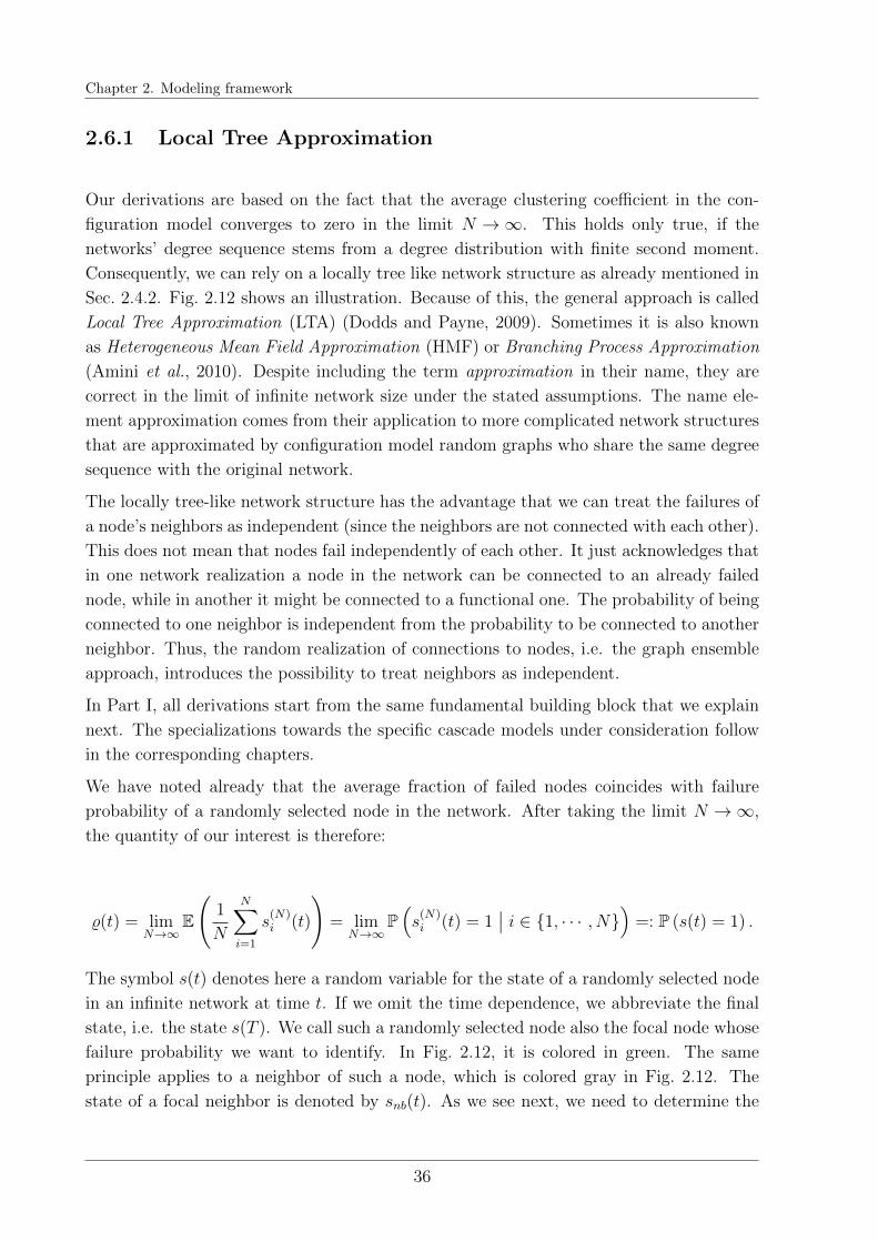
Chapter 2. Modeling framework
2.6.1 Local Tree Approximation
Our derivations are based on the fact that the average clustering coefficient in the con-
figuration model converges to zero in the limit N →∞. This holds only true, if the
networks’ degree sequence stems from a degree distribution with finite second moment.
Consequently, we can rely on a locally tree like network structure as already mentioned in
Sec. 2.4.2. Fig. 2.12 shows an illustration. Because of this, the general approach is called
Local Tree Approximation (LTA) (Dodds and Payne, 2009). Sometimes it is also known
as Heterogeneous Mean Field Approximation (HMF) or Branching Process Approximation
(Amini et al., 2010). Despite including the term approximation in their name, they are
correct in the limit of infinite network size under the stated assumptions. The name ele-
ment approximation comes from their application to more complicated network structures
that are approximated by configuration model random graphs who share the same degree
sequence with the original network.
The locally tree-like network structure has the advantage that we can treat the failures of
a node’s neighbors as independent (since the neighbors are not connected with each other).
This does not mean that nodes fail independently of each other. It just acknowledges that
in one network realization a node in the network can be connected to an already failed
node, while in another it might be connected to a functional one. The probability of being
connected to one neighbor is independent from the probability to be connected to another
neighbor. Thus, the random realization of connections to nodes, i.e. the graph ensemble
approach, introduces the possibility to treat neighbors as independent.
In Part I, all derivations start from the same fundamental building block that we explain
next. The specializations towards the specific cascade models under consideration follow
in the corresponding chapters.
We have noted already that the average fraction of failed nodes coincides with failure
probability of a randomly selected node in the network. After taking the limit N →∞,
the quantity of our interest is therefore:
%(t) = limN→∞
E
(1
N
N∑i=1
s(N)i (t)
)= lim
N→∞P(s
(N)i (t) = 1
∣∣ i ∈ 1, · · · , N) =: P (s(t) = 1) .
The symbol s(t) denotes here a random variable for the state of a randomly selected node
in an infinite network at time t. If we omit the time dependence, we abbreviate the final
state, i.e. the state s(T ). We call such a randomly selected node also the focal node whose
failure probability we want to identify. In Fig. 2.12, it is colored in green. The same
principle applies to a neighbor of such a node, which is colored gray in Fig. 2.12. The
state of a focal neighbor is denoted by snb(t). As we see next, we need to determine the
36

2.6. Analytic Framework
Figure 2.12: Illustration of the local tree approximation. The green node is the focalnode. Its conditional failure probability P(s = 1|k = 5) can be computed according toEquation (2.1), and depends on the state of its neighbors: Here, the two red ones andthe gray one have failed, while the two blue ones are still functional. The neighbors’conditional failure probabilities P(snb = 1|k) rely on the failure probabilities of their ownneighbors without regarding the green focal point.
failure probability of such a neighbor, because s(t) depends on it.
Failure probability of a node
We recall that the failure of a node is determined by two (random) variables: its threshold
Θ and its fragility Λ(t), i.e. the load that it carries at time (t). Whenever the carried load
exceeds its threshold, a node fails. Thus, we can deduce the relation:
%(t) = P (Θ ≤ Λ(t)) .
We know that Λ(t) sums up the load that a focal node has received by its failed neighbors
in the course of the cascade. Consequently, it depends on the degree K of a node. From
Bayes’ Theorem (Feller, 1968), it follows:
%(t) =c∑
k=1
p(k)P(s(t) = 1
∣∣ k) =c∑
k=1
p(k)P(Θ ≤ Λ(t)
∣∣ k) ,
37

Chapter 2. Modeling framework
where P(s(t) = 1
∣∣ k) denotes the conditional failure probability of a node given that its
degree is K = k. We also write Λ(k, t) and Θ(k) to indicate that the distributions of Λ(t)
and Θ can depend on the degree k of a node.
Conditional failure probability
The k neighbors of this focal node with degree k have distributed at time t− 1 or before
a random load Lnb(k, t− 1) independently of each other. The distribution is independent
because of the locally tree-like network structure. If a neighbor is not failed yet or does
not distribute any load, it simply distributes zero load, i.e. Lnb(k, t − 1) = 0. Thus, we
can assign to each neighbor j = 1, · · · , k a random variable Lnbj (k, t − 1) ∼ Lnb(k, t − 1).
These random variables are iid and sum up to Λ(k, t):
Λ(k, t) =k∑j=1
Lnbj (k, t− 1).
Since the random variables are independent, their sum is distributed as the convolution
of their distributions.1 As they are identically distributed, this simplifies to the k-fold
convolution: Λ(k, t) ∼ p∗kLnb(k,t−1)
.
In summary, we have deduced:
P(s(t) = 1
∣∣ k) = P (Θ(k) ≤ Λ(k, t)) = P
(Θ(k) ≤
k∑j=1
Lnbj (k, t− 1)
)
=
∫ ∞0
FΘ(k) (x) p∗kLnb(k,t−1)(x) dx.
(2.1)
Consequently, the task is left to derive an analytic expression for the load Lnb(k, t) that a
single neighbor distributes to a node with degree k.
Failure probability of a neighbor
The first step on this way is guided by the insight that the fragility of a focal neighbor
Λ(nb)(t), i.e. the load that it carries, is of similar form as the one of a node. The only
difference is that we want to calculate the distribution of Λ(nb)(t) conditional on the fact
that one of its neighbors, i.e., the focal node, has not failed yet. The failure of the focal
node can only be caused by failures of neighbors that have distributed their load before
1In case of degree-degree correlations (i.e. correlations between the degree K of a node and its neighborKnb this would still be true. Only in case of correlations between the degrees of the neighbors, more effortwould be needed to calculate the distribution of the sum of dependent variables.)
38
2.6. Analytic Framework
the failure of the node. This property of a neighbor whose failure does not regard the focal
node is called the Without Regarding Property (WOR) by Hurd and Gleeson (2013).
With this in mind, we can thus write:
P(snb(t) = 1
∣∣ k) = P(Θ(k) ≤ Λnb(k, t)
)= P
(Θ(k) ≤
k−1∑j=1
Lnbj (k, t− 1)
)
=
∫ ∞0
FΘ(k) (x) p∗(k−1)
Lnb(k,t−1)(x) dx.
(2.2)
A second important difference between a node and a neighbor needs to be mentioned. A
neighbors degree Knb does not follow the pdf p(k) as the one of a node. Instead, we have:
pnb(k) := P(Knb = k
)=p(k)k
z, (2.3)
where z :=∑
k kp(k) denotes the normalizing average degree. pnb(k) is proportional to the
degree k in the configuration model, because each of a neighbor’s k links could possibly
connect the neighbor with the focal node (see, e.g., Newman (2010)). Thus, a node with
a higher degree has a higher chance to be connected with the focal node.
Now, Bayes’ Theorem provides an expression for the failure probability π(t) := P (snb(t) = 1)
of a neighbor:
π(t) =c∑
k=1
pnb(k)P(snb(t) = 1
∣∣ k) =c∑
k=1
pnb(k)
∫ ∞0
FΘ(k) (x) p∗(k−1)
Lnb(k,t−1)(x) dx. (2.4)
With this definition, we can go even further. The following derivation is useful to under-
stand the relation between our work and the state of the art of LTAs. Let’s denote with
Lfnb(k, t− 1) the random load that a single neighbor distributes to a node with degree k
conditional on the event that the neighbor has failed before or at time t− 1. Since neigh-
bors of a node fail independently, the number Nf of failed neighbors out of k neighbors
is simply binomial distributed. We abbreviate the probability for the event that exactly
Nf = n neighbors are failed as
b(n, k, π(t− 1)) :=
(k
n
)π(t− 1)n(1− π(t− 1))k−n.
39

Chapter 2. Modeling framework
Then, an alternative to Eq. (2.2) reads as:
P(snb(t) = 1
∣∣ k) =k−1∑n=0
P (Nf = n)P
(Θ(k) ≤
k−1∑j=1
Lnbj (k, t− 1)∣∣ Nf = n
)
=k−1∑n=0
b(n, k − 1, π(t− 1))P
(Θ(k) ≤
n∑j=1
Lnbfj (k, t− 1)
)
=k−1∑n=0
b(n, k − 1, π(t− 1))
∫ ∞0
FΘ(k) (x) p∗nLfnb(k,t−1)(x) dx.
(2.5)
With these preparations, we are ready to shift our focus to a more detailed exploration of
our three model classes.
40
Chapter 3
Diversification strategies in Constant
Load models
Summary
We study the influence of risk diversification on cascading failures originatingfrom Constant Load models in weighted complex networks, where weighteddirected links represent exposures between nodes. These weights result fromdifferent diversification strategies and their adjustment allows to reduce sys-temic risk significantly by topological means. As example, we contrast a clas-sical Exposure Diversification (ED) approach with a Damage Diversification(DD) variant. The latter reduces the loss that the failure of high degree nodesgenerally inflict to their network neighbors and thus hampers the cascade am-plification. To quantify the final cascade size and obtain our results, we developa branching process approximation taking into account that inflicted losses cannot only depend on properties of the exposed, but also of the failing node. Thisanalytic extension is a natural consequence of the paradigm shift from individ-ual to system safety. To deepen our understanding of the cascade process, wecomplement this systemic perspective by a mesoscopic one: an analysis of thefailure risk of nodes dependent on their degree. Additionally, we ask for therole of these failures in the cascade amplification.
Based on R. Burkholz, A. Garas, and F. Schweitzer, “How damage diversification can reduce systemicrisk”. Physical Review E 93, 042313. RB contributed to the design of the research questions, derivedthe analytic equations, implemented the code, interpreted the results and wrote the main part of themanuscript. A description of the cascade dynamics has been added specifically for this thesis.
41
Chapter 3. Diversification strategies in Constant Load models
3.1 Introduction
We devote this chapter to a closer analysis of the two Constant Load model variants that
we introduced in Sec. 2.3.1. As we have seen already, CL models are strongly linked to
the network structure. The loss lji that a node i experiences in case of the failure of its
neighbor j can be interpreted as weight of the link (j, i). Consequently, systemic risk is to
a large extend determined by the interconnectivity properties and dependence structure
of the studied system.
Increased dependence, under normal conditions, has advantages for the efficient operation
of a system. It also leads to an increased risk diversification of its components, since the
dependence on single other components is reduced. According to classical risk management
theories (Allen and Gale, 2000) a higher connectivity thus decreases the vulnerability of
the system as a whole, even with respect to cascading failures. Several authors, e.g. (Allen
et al., 2011; Battiston et al., 2012b; Gai and Kapadia, 2010; Gleeson and Cahalane, 2007;
Roukny et al., 2013), pointed already out that a higher connectivity can also increase
systemic risk, i.e. in our context the expected cascade size.
Although these findings are partially model-dependent, they can be explained intuitively
by a basic trade-off between diversification and system connectivity that is reflected in the
risk exposures. In fact, most of these works are based on a cascade model by Watts (2002),
the ED model, which introduces this trade-off, and can be interpreted as a study of simple
diversification strategies of system components or agents that are represented as nodes in
a network. Increased diversification of system components reduces their exposure to the
failure of single other components. But at the same time, it increases the connectivity of
the overall system. Especially, if well connected components, so called hubs, fail they affect
a high number of other nodes. Even if the inflicted damage is only little, if it is enough
to trigger a few other failures, the cascade might continue and span a large fraction of the
entire system.
This implies that hubs, because of their large number of neighbors, considerably affect the
network in case of failure. Consequently, policy discussions and risk reduction strategies
center around the question of how to prevent the failure of hubs, e.g. by increasing
their robustness. Examples include relative capital buffers in finance (Arinaminpathy
et al., 2012; Roukny et al., 2013) or immunization in epidemiology (Pastor-Satorras and
Vespignani, 2002).
Here, we test in a generic modeling approach a way to complement such regulatory efforts
and strategies by the mitigation of the impact of the failures of well connected nodes
as it is realized in the DD model. In the DD model, the impact of a failing node in a
network is diversified instead of its exposures. This has the potential to reduce systemic
risk significantly, since the failure amplification caused by hubs is counterbalanced. For
42
3.1. Introduction
instance, in a financial network this approach would correspond to a policy where each
financial institution is only allowed to get into a limited amount of debt. We are aware
that our approach is abstract, and it is based on simplifying assumptions that deviate
from real world application scenarios. However, we do hope to motivate researchers in
more applied fields and practitioners to consider topological possibilities that can reduce
systemic risk.
In this chapter, we present analytic derivations for network ensemble averages as described
in Sec. 2.4. The simulation results of Sec. 2.5 serve as benchmark to provide evidence that
our approximations are correct. Additionally, we present the dynamics of the cascade
size for specific threshold values that we obtained by simulations as well as our analytic
approach.
Recall that these derivations are valid in the limit of infinite network size, where two quan-
tities on the system level are given: a) the degree distribution, which defines the number
of direct neighbors of a node, and thus limits their respective diversification strategies,
and b) the threshold distribution defining the robustness of nodes.
We build on the work of Gleeson and Cahalane (2007) who have derived the LTA for the
ED model. However, this approach does not capture processes where the impact of a
failing neighbor depends on its specific properties (e.g., its degree or robustness) as it is
required for the treatment of the DD variant. Therefore, we extend the branching process
approximation to the latter case, and generalize it for the application to weighted random
network models. The weight statistics could be deduced from data, taking also into account
different properties of neighboring nodes, or from specific model assumptions. This way,
we generalize the analytic treatment to match application scenarios better. Moreover, it
allows to deepen the understanding of the role of different risk diversification strategies. In
fact, it translates a recent paradigm shift to an analytic setting. The focus has been shifted
from individual or component-wise risk assessments to systemic risk analysis. Thus, the
question of the failure risk of single components is complemented by the question for the
consequences of their failure for the rest of the system. A systemic risk analysis is often
accompanied by the identification of so-called system-relevant nodes. But this analysis
is based on the assumption that various components can have a different impact on the
system stability. This is considered in our framework, as failing nodes can cause different
damage to their network neighbors.
As a result of the trade-off between system connectivity and risk diversification an in-
creased diversification does not need to reduce the failure risk neither of the system nor
its components. Increased diversification does not even need to decrease the failure risk
of a component despite the fact that it reduces systemic risk.
Because of this, we accompany our systemic risk measure on the macro-level, the average
cascade size, with a comparison of failure probabilities of nodes with different diversifica-
43
Chapter 3. Diversification strategies in Constant Load models
tion strategies on the meso-level. The nodes’ systemic relevance can then be identified on
the basis of their cascade amplification role.
3.2 Local Tree Approximation
As expansion of the network and threshold ensembles introduced in Sec. 2.4, we assume
that the links between nodes have weights wij as introduced in Sec. 2.4.2. These weights
define the losses lij = wij that nodes inflict on each other in case of their failure. In general,
they can be expressed as independent random variables Wij, which follow distributions
that can depend on the degrees of the start and end node of the link: Wij ∼ pW (ki,kj). In
the beginning of each cascade, the weights are drawn independently at random, after the
degrees and thresholds of the nodes have been fixed, and stay constant over the course of
the cascade.
This way, a direction of a link is introduced, since in general we can have wij 6= wji. Still,
we can assume an undirected skeleton network, i.e., we do not need to distinguish between
in-degrees and out-degrees. This differs from the usual approach for directed networks
(Amini et al., 2010, 2012; Gai and Kapadia, 2010) where the neighbors whose failures
impact a node are distinct from the ones who face a loss in case of the node’s failure. In
this case, one node is exposed to the other, but not vice versa. In our case, however, once
there is a link between two nodes, each can impact the other, but the amount of the loss
can be different. Still, this does not limit us to the study of undirected networks, since
weights wji in one direction can also be set to zero (wji = 0). Instead, it allows us to model
situations where some nodes are part of mutual dependencies as well as one way exposures.
Thus, our approach is a generalization. In Appendix A.4, we provide an example for an
exclusively directed network by defining the weights as net difference between weights in
the DD approach: w(eff)ji = max (1/kj − 1/ki, 0).
Some special choices of weights and networks with other weight statistics have been con-
sidered already.
3.2.1 The state of the art
For the ED approach, the average fraction of failed nodes at the end of a cascade can be
calculated on random networks with given degree distribution p(k) and threshold distri-
bution FΘ(θ) (Gleeson and Cahalane, 2007). This LTA were studied in many subsequent
works. It was generalized for directed and undirected weighted networks (Amini et al.,
2010; Hurd and Gleeson, 2013), it was found to be accurate even for several clustered
networks with small mean inter-vertex distance (Melnik et al., 2011), and the influence
of degree-degree correlations has been investigated (Dodds and Payne, 2009; Payne et al.,
44
3.2. Local Tree Approximation
2009). According to a general framework introduced by Lorenz et al. (2009), the ED and
DD approach belong to the constant load class, where the ED is called the inward variant,
while the DD is identified as the outward variant. Still, the risk reduction potential of the
latter has not been understood so far, since a system’s exposure to systemic risk has been
only explored on fully-connected (Lorenz et al., 2009) or regular (Battiston et al., 2012a;
Gleeson and Cahalane, 2007; Lorenz et al., 2009) networks, where both model variants
coincide.
In order to study the DD approach on more general networks, we generalized and extended
the existing approximations, which were proven to be exact for the case of ED (Amini
et al., 2010; Hurd and Gleeson, 2013). Now, we can treat more general processes where
the directed weights in a directed or undirected network can depend on properties of both
nodes, the failing as well as the loss facing one. Here, in contrast to Ref.(Amini et al.,
2010), nodes can depend on each other and properties of the failing node influence the
amount of loss faced, and in contrast to Ref.(Hurd and Gleeson, 2013) nodes can depend
on each other in a non-symmetric way. Moreover, the insight that the iterative steps in
the fixed point iteration that lead to the final cascade size correctly desribe the cascade
dynamics seems to be new.
We show in Section 3.3 that our approach leads to very good agreements with simulations
on finite Poisson and scale free random graphs. Many large systems belong to the latter
class (Barabasi, 2009; Caldarelli, 2007; Cohen and Havlin, 2010). But often, simulations
would require more computational time than our analytic approach or would even be im-
possible, because nodes with degree far in the right tail of the degree distribution are only
realized in large networks that most times cannot be sampled with adequate accuracy. In-
terestingly, very sparse networks seem to reduce systemic risk for most parameters because
of their low connectivity. An example for such a case is provided in the Appendix.
First, we derive the LTA of the cascade size for random graph ensembles with general
weight distributions as explained.
3.2.2 Analytic approach for general weighted networks
In Sec. 2.6.1, we have derived an expression for the cascade size %(t) that finally depends
on the conditional failure probability of a focal neighbor as provided by Eq. (2.2). We
recall that it is of the form
P(snb(t) = 1
∣∣ k) = P
(Θ(k) ≤
k−1∑j=1
Lnbj (k, t− 1)
).
The task is left to derive the distribution of the load Lnbj (k, t−1) that a focal neighbor has
distributed before or at time t− 1 to a focal node or neighbor with degree k. Both a focal
45
Chapter 3. Diversification strategies in Constant Load models
neighbor and a focal node are illustrated in Fig. 2.12 in gray and green respectively. We
assume throughout this chapter that the load Lnbj (k, t− 1) is a discrete random variable.
All our derivations work analogously for the densities of continuous random variables.
We would need to discretize them in numerical calculations anyway. Because of this, we
restrict ourselves to the discrete case.
The load distributed by neighbors
Because of the constant load assumption, the load that a failed neighbor distributes in case
of its failure is constant over time and is defined by the distributions of the weights Wji
that define the load that a failed neighbor distributes. We assume that these distributions
are known for given degrees of the nodes that are adjacent to a given weighted link. For
instance, if kj = d and ki = k, we know that Wji ∼ W (d, k). This load is distributed only,
if a failed neighbor has degree d. However, a neighbor can be in one of two states: it is
failed with probability π(t − 1) and distributes load or it is functional with probability
1− π(t− 1). Thus Bayes’ Theorem leads us to
P(Lnb(k, t− 1) = l
)= (1− π(t− 1))P
(Lnb(k, t− 1) = l
∣∣ snb(t− 1) = 0)
+ π(t− 1)P(Lnb(k, t− 1) = l
∣∣ snb(t− 1) = 1).
for any l ∈ R. It is certain that a neighbor does not distribute any load, if it has not failed
yet. Thus, the probability P(Lnb(t− 1) = l
∣∣ snb(t− 1) = 0)
to distribute any load l 6= 0
in case that the neighbor is not failed is zero and it is 1 otherwise. We can determine
π(t− 1) with the help of (Eq. 2.4). So, we can focus on the case in which the neighbor is
failed and distributes load.
The question that we need to answer is: What is the probability pfnb(d) that a failed
neighbor j has degree d? The probability does not exactly follow the neighbor’s degree
distribution pnb(d), since some nodes with a given degree might have a higher failure
probability than others and would be thus underrepresented, if we would randomly select
a neighbor in the network. In fact, we restrict ourselves to sample from the failed neighbors
and ask for the probability that its degree is d. Thus, failed neighbors with degree d are
represented in this sample proportionally to their failure probability P(snb(t− 1) = 1∣∣ d).
The correct distribution of the degree Kfnb of a failed neighbor at time t− 1 follows from
Bayes’ Theorem:
pfnb(d) = P(Kfnb = d
)=
P(snb(t− 1) = 1∣∣ d)p(d)d
zπ(t− 1).
Again employing Bayes’ Theorem lets us deduce the distribution of the loss that a neighbor
46

3.2. Local Tree Approximation
inflicts in case of its failure:
P(Lnb(k, t− 1) = l∣∣ snb(t− 1) = 1) =
=c∑
d=1
pfnb(d)P(Lnb(k, t− 1) = l
∣∣ snb(t− 1) = 1, Kfnb = d)
=c∑
d=1
pfnb(d)P (W (d, k) = l)
for any l ∈ R.
In summary, we define the pdf pLnb(k,t−1)(l) := P(Lnb(k, t− 1) = l
)as:
P(Lnb(k, t− 1) = 0
)= (1− π(t− 1)) +
+c∑
d=1
P(snb(t− 1) = 1∣∣ d)p(d)d
zP (W (d, k) = 0)
P(Lnb(k, t− 1) = l
)=
c∑d=1
P(snb(t− 1) = 1∣∣ d)p(d)d
zP (W (d, k) = l) .
(3.1)
for l 6= 0.
The first factor simply corresponds to the probability that a neighbor has degree d and is
failed, while the second factor describes the probability that such a node distributes the
load l.
Then, the sum of k − 1 independent copies of Lnb(t− 1) is distributed by the (k − 1)-fold
convolution of this variable. Therefore, we have deduced the missing building blocks to
define the dynamics of the fraction of failed nodes %(t) by
P(snb(t) = 1
∣∣ k) = P
(Θ(k) ≤
k−1∑j=1
Lnbj (k, t− 1)
)=∑x
FΘ(k) (x) p∗(k−1)
Lnb(k,t−1)(x), (3.2)
P(s(t) = 1
∣∣ k) = P
(Θ(k) ≤
k∑j=1
Lnbj (k, t− 1)
)=∑x
FΘ(k) (x) p∗(k)
Lnb(k,t−1)(x). (3.3)
so that we obtain:
%(t) =c∑
k=1
p(k)P(s(t) = 1
∣∣ k) .The right hand side in the definition of the conditional failure probability of a neighbor
P(snb(t) = 1
∣∣ k) in Eq. (3.2) can also be interpreted as the k-th component of a vector
valued function G : [0, 1]c → [0, 1]c that maps the conditional failure probabilities at time
t − 1 to the corresponding values at time t. This is possible, since the distribution of
47
Chapter 3. Diversification strategies in Constant Load models
Lnb(k, t− 1) is solely defined by the knowledge of the vector
PPP(snb = 1∣∣ k) :=
(P(snb = 1
∣∣ k))k∈1,··· ,c ∈ [0, 1]c.
For any q ∈ [0, 1]c, we define the k-th component Gk(qqq) of G(q) as:
Gk(qqq) :=∑x
FΘ(k) (x) p∗(k−1)L(qqq) (x),
or for continuously distributed L(qqq) and weights as:
Gk(qqq) :=
∫ ∞0
FΘ(k) (x) p∗(k−1)L(qqq) (x) dx,
where pL(q) is defined analogously to Eq. (3.1) as:
pL(qqq)(0) =1−c∑
d=1
qd p(d)d
z+
c∑d=1
qd p(d)d
zpW (d,k)(0),
pL(qqq)(l) =c∑
d=1
qd p(d)d
zpW (d,k)(l) for l 6= 0.
Although we do not state the k dependence explicitly, we note that for each k we can have
a different L(qqq).
With this definition, we can formulate Eq. (3.2) equivalently as:
PPP(snb(t) = 1∣∣ k) = GGG
(PPP(snb(t− 1) = 1
∣∣ k)). (3.4)
Consequently, the cascade process converges to a steady state for t → ∞, if the function
G : [0, 1]c → [0, 1]c attains a fixed point.
Such a fixed point PPP(snb = 1∣∣ k) exists according to the Knaster-Tarski Theorem (Tarski,
1955), since the function G is monotone with respect to a partial ordering and maps the
complete lattice [0, 1]c onto itself.1 A proof is given in Appendix A.1.
In the models considered, numerical convergence is achieved the latest after t = 50 fixed
point iterations that are equivalent to time steps in the cascade process.
After these steps, we estimate our measure of systemic risk
% = limt→∞
%(t),
the final fraction of failed nodes.
1Definition of the partial ordering: Two vectors x, y ∈ [0, 1]c
are ordered as x ≤ y, if and only ifxi≤yi holds for all their components i ∈ I.
48
3.2. Local Tree Approximation
Simplification for homogeneous failure probability of neighbors
In case the impact of a failing neighbor does not depend on its degree d, i.e. W (d, k) ∼W (k), the vector valued fixed point equation Eq. (3.4) simplifies to a scalar fixed point
equation.
To see this, we first observe that Eq. (3.1) reads for l 6= 0 in the steady state t→∞ as:
P(Lnb(k) = l
)= P (W (k) = l)
c∑d=1
P(snb = 1∣∣ d)p(d)d
z= P (W (k) = l)π
and for l = 0 we have P(Lnb(k) = 0
)= 1−π+πP (W (k) = 0). Thus, the load distribution
does not depend on all the different failure probabilities of neighbors with a given degree d
anymore. Instead, the failure probability π of a randomly selected neighbor defines already
the load distribution by a neighbor. Thus, we only need to determine π. To give better
prominence to the dependence of P(snb = 1
∣∣ k) on π, we write it in the form of Eq. (2.5).
Thus, we consider distributions of the load Lfnb(k) that a neighbor distributes to a focal
node or neighbor with degree conditional on the fact that it is failed. We simply obtain:
P(Lfnb(k) = l
)= P
(Lnb(k) = l
∣∣ snb = 1)
= P (W (k) = l) .
Thus, Lfnb(k) and W (k) are identical distributed. As consequence, Lfnb(k) does not even
depend on π anymore and its distribution stays constant for the whole cascade. According
to Eq. (2.5), we can thus factorize the conditional failure probability of a neighbor in one
part that captures the π dependence and another part that stays constant in each iteration
step.
P(snb(t) = 1
∣∣ k) =k−1∑n=0
b(n, k − 1, π)P
(Θ(k) ≤
n∑j=1
Wj(k)
).
With Eq. (2.4), we arrive at the promised scalar valued fixed point equation:
π =c∑
k=1
pnb(k)P(snb(t) = 1
∣∣ k) =c∑
k=1
pnb(k)k−1∑n=0
b(n, k − 1, π)P
(Θ(k) ≤
n∑j=1
Wj(k)
),
(3.5)
whose solution is enough to calculate the final fraction of failed nodes as
% =∑k
p(k)k∑
n=0
b(n, k, π)P
(Θ(k) ≤
n∑j=1
Wj(k)
), (3.6)
49
Chapter 3. Diversification strategies in Constant Load models
where we have used:
P(s = 1
∣∣ k) =k∑
n=0
b(n, k, π)P
(Θ(k) ≤
n∑j=1
Wj(k)
), (3.7)
For general weight distributions, this equation is not known from the literature. But
Amini et al. (2010) have derived the final cascade size distribution for weighted networks
on directed skeleton networks, while Dodds and Payne (2009); Gleeson and Cahalane
(2007) came to this equation for a special choice of weights, i.e. the ED model.
Despite its generality, this simpler approach is not able to capture the cascade dynamics
of the damage diversification model.
3.2.3 Specialization to ED and DD models
The only piece missing to calculate the final cascade size for the ED and DD models is
the specification of the weight distributions pW (d,k).
In both cases, the weights are completely deterministic. We have:
P(W (ED)(d, k) = l
)= δ1/k(l), P
(W (DD)(d, k) = l
)= δ1/d(l),
where δy(x), defined as δy(x) := 1 if x = y and δy(x) := 0 otherwise, denotes the discrete
delta distribution.
We note that W (ED)(d, k) = W (ED)(k) is independent of the degree d of a neighbor that
can potentially inflict the loss 1/k to a focal node or neighbor with degree k. Consequently,
the calculation of the average final fraction of failed nodes can be simplified as outlined in
the previous section. Specifically, because of W (ED)(d, k) = W (ED)(k) ∼ δ1/k, we have
P
(Θ(k) ≤
n∑j=1
W(ED)j (d, k)
)= P
(Θ(k) ≤
n∑j=1
1
k
)= FΘ(k)
(nk
). (3.8)
Thus, the fixed point equation Eq. (3.5) specializes to
π(ED) =c∑
k=1
pnb(k)k−1∑n=0
b(n, k − 1, π(ED))FΘ(k)
(nk
). (3.9)
This coincides with the derivations by Gleeson and Cahalane (2007), if the threshold Θ(k)
is independent of the degree k of the focal neighbor.
For the DD case, we note that the weights are independent of the degree k of the potentially
load receiving focal node or neighbor, i.e. W (d, k) = W (d). Also this aspect leads to a
50
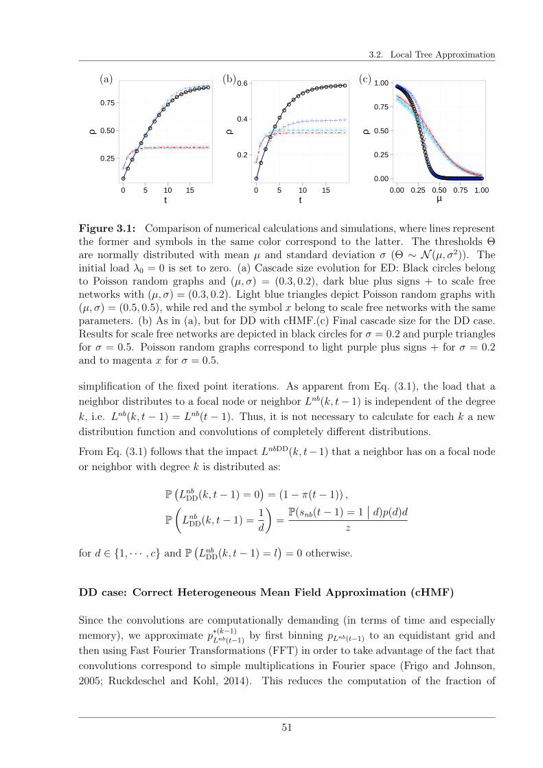
3.2. Local Tree Approximation
0.25
0.50
0.75
0 5 10 15t
ρ
0.2
0.4
0.6
0 5 10 15t
ρ
0.00
0.25
0.50
0.75
1.00
0.00 0.25 0.50 0.75 1.00µ
ρ
(a) (b) (c)
Figure 3.1: Comparison of numerical calculations and simulations, where lines representthe former and symbols in the same color correspond to the latter. The thresholds Θare normally distributed with mean µ and standard deviation σ (Θ ∼ N (µ, σ2)). Theinitial load λ0 = 0 is set to zero. (a) Cascade size evolution for ED: Black circles belongto Poisson random graphs and (µ, σ) = (0.3, 0.2), dark blue plus signs + to scale freenetworks with (µ, σ) = (0.3, 0.2). Light blue triangles depict Poisson random graphs with(µ, σ) = (0.5, 0.5), while red and the symbol x belong to scale free networks with the sameparameters. (b) As in (a), but for DD with cHMF.(c) Final cascade size for the DD case.Results for scale free networks are depicted in black circles for σ = 0.2 and purple trianglesfor σ = 0.5. Poisson random graphs correspond to light purple plus signs + for σ = 0.2and to magenta x for σ = 0.5.
simplification of the fixed point iterations. As apparent from Eq. (3.1), the load that a
neighbor distributes to a focal node or neighbor Lnb(k, t− 1) is independent of the degree
k, i.e. Lnb(k, t − 1) = Lnb(t − 1). Thus, it is not necessary to calculate for each k a new
distribution function and convolutions of completely different distributions.
From Eq. (3.1) follows that the impact LnbDD(k, t−1) that a neighbor has on a focal node
or neighbor with degree k is distributed as:
P(LnbDD(k, t− 1) = 0
)= (1− π(t− 1)) ,
P(LnbDD(k, t− 1) =
1
d
)=
P(snb(t− 1) = 1∣∣ d)p(d)d
z
for d ∈ 1, · · · , c and P(LnbDD(k, t− 1) = l
)= 0 otherwise.
DD case: Correct Heterogeneous Mean Field Approximation (cHMF)
Since the convolutions are computationally demanding (in terms of time and especially
memory), we approximate p∗(k−1)
Lnb(t−1)by first binning pLnb(t−1) to an equidistant grid and
then using Fast Fourier Transformations (FFT) in order to take advantage of the fact that
convolutions correspond to simple multiplications in Fourier space (Frigo and Johnson,
2005; Ruckdeschel and Kohl, 2014). This reduces the computation of the fraction of
51
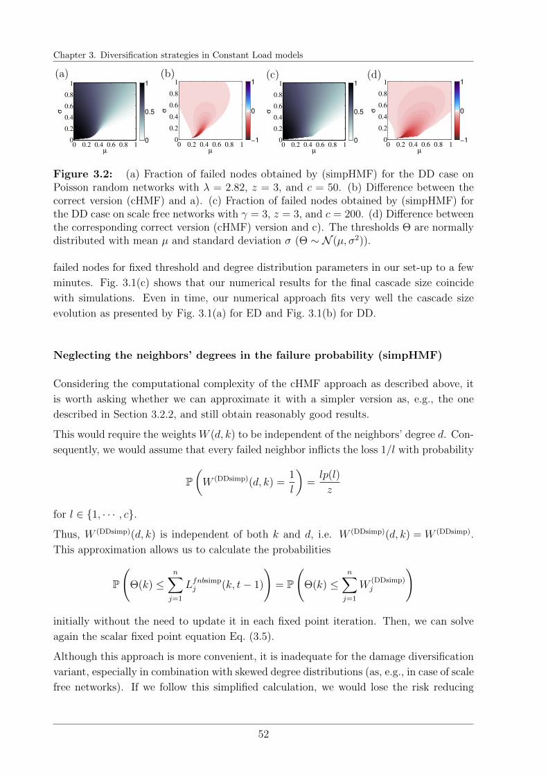
Chapter 3. Diversification strategies in Constant Load models
µ
σ
0 0.2 0.4 0.6 0.8 10
0.2
0.4
0.6
0.8
1
0
0.5
1
µ
σ
0 0.2 0.4 0.6 0.8 10
0.2
0.4
0.6
0.8
1
−1
0
1
µ
σ
0 0.2 0.4 0.6 0.8 10
0.2
0.4
0.6
0.8
1
0
0.5
1
µ
σ
0 0.2 0.4 0.6 0.8 10
0.2
0.4
0.6
0.8
1
−1
0
1
(a) (b) (c) (d)
Figure 3.2: (a) Fraction of failed nodes obtained by (simpHMF) for the DD case onPoisson random networks with λ = 2.82, z = 3, and c = 50. (b) Difference between thecorrect version (cHMF) and a). (c) Fraction of failed nodes obtained by (simpHMF) forthe DD case on scale free networks with γ = 3, z = 3, and c = 200. (d) Difference betweenthe corresponding correct version (cHMF) version and c). The thresholds Θ are normallydistributed with mean µ and standard deviation σ (Θ ∼ N (µ, σ2)).
failed nodes for fixed threshold and degree distribution parameters in our set-up to a few
minutes. Fig. 3.1(c) shows that our numerical results for the final cascade size coincide
with simulations. Even in time, our numerical approach fits very well the cascade size
evolution as presented by Fig. 3.1(a) for ED and Fig. 3.1(b) for DD.
Neglecting the neighbors’ degrees in the failure probability (simpHMF)
Considering the computational complexity of the cHMF approach as described above, it
is worth asking whether we can approximate it with a simpler version as, e.g., the one
described in Section 3.2.2, and still obtain reasonably good results.
This would require the weights W (d, k) to be independent of the neighbors’ degree d. Con-
sequently, we would assume that every failed neighbor inflicts the loss 1/l with probability
P(W (DDsimp)(d, k) =
1
l
)=lp(l)
z
for l ∈ 1, · · · , c.
Thus, W (DDsimp)(d, k) is independent of both k and d, i.e. W (DDsimp)(d, k) = W (DDsimp).
This approximation allows us to calculate the probabilities
P
(Θ(k) ≤
n∑j=1
Lfnbsimpj (k, t− 1)
)= P
(Θ(k) ≤
n∑j=1
W(DDsimp)j
)
initially without the need to update it in each fixed point iteration. Then, we can solve
again the scalar fixed point equation Eq. (3.5).
Although this approach is more convenient, it is inadequate for the damage diversification
variant, especially in combination with skewed degree distributions (as, e.g., in case of scale
free networks). If we follow this simplified calculation, we would lose the risk reducing
52

3.3. Numerical Results
effect by hubs connected to more nodes. This would lead us to draw opposite conclusions
about systemic risk. So, as shown in Fig. 3.2, it is crucial to use the correct HMF to explain
our simulation results. The simplified method simpHMF leads to an overestimation of the
final fraction of failed nodes.
3.3 Numerical Results
Hereafter, we show how the DD variant can reduce systemic risk in comparison to the
ED variant by calculating the fraction of failed nodes for both variants and several degree
distributions. Alongside, we study the influence of the presence of hubs and the degree
variance. This allows us to discuss up to which extend the overall diversification reduces
or increases systemic risk. Later on, we also compare how a higher or lower diversification
influences the failure risk of a node on the mesoscopic level.
Our findings do not only lead to different conclusions for the two model variants, but also
depend on the threshold distribution parameters under consideration.
Similar to Refs.(Watts, 2002) and (Gleeson and Cahalane, 2007) we study normally dis-
tributed thresholds Θ ∼ N (µ, σ2) with mean µ and standard deviation σ, but we explore
the role of the thresholds’ heterogeneity as well as their mean size more extensively by
providing a 2d-phase diagram as in Ref.(Lorenz et al., 2009). Although our analytic frame-
work also applies to more general cases, here we assume the thresholds to be independent
from the degree k of a node.
Recall that the initial fraction of failed nodes is determined by the nodes with negative
thresholds (Θ ≤ 0) and is thus given by FΘ(0) = Φ(−µσ
), where Φ denotes the cumulative
distribution function of the standard normal distribution.
3.3.1 Systemic perspective
In principle, all phase diagrams are of similar shape as the one for fully connected networks
of infinite size that has been calculated in Ref.(Lorenz et al., 2009) and is depicted in
Fig. 3.3 (a). It shows the effect of perfect diversification. Both variants, ED and DD,
coincide for this case as well as for regular networks where every node has the same degree
z.
We observe that increasing the standard deviation can also reduce systemic risk - even
though this increases the fraction of initial failures. Of special prominence is the sharp
regime shift from a region of small systemic risk to an almost complete system break-
down. The existence of such a regime shift has been first identified for Poisson random
graphs and the ED variant by Gleeson and Cahalane (2007). It is present for most other
53
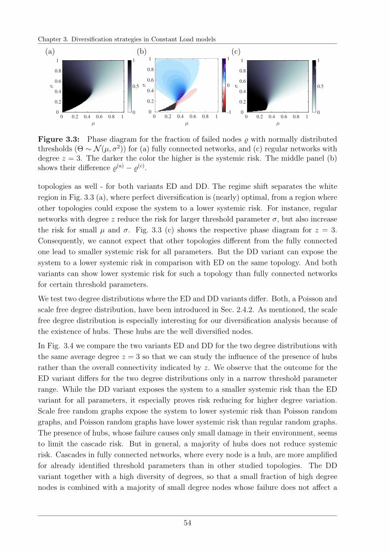
Chapter 3. Diversification strategies in Constant Load models
µ
0 0.2 0.4 0.6 0.8 1
σ
0
0.2
0.4
0.6
0.8
1
0
0.5
1
µ
0 0.2 0.4 0.6 0.8 1
σ
0
0.2
0.4
0.6
0.8
1
-1
0
1
µ
0 0.2 0.4 0.6 0.8 1
σ
0
0.2
0.4
0.6
0.8
1
0
0.5
1
(a) (b) (c)
Figure 3.3: Phase diagram for the fraction of failed nodes % with normally distributedthresholds (Θ ∼ N (µ, σ2)) for (a) fully connected networks, and (c) regular networks withdegree z = 3. The darker the color the higher is the systemic risk. The middle panel (b)shows their difference %(a) − %(c).
topologies as well - for both variants ED and DD. The regime shift separates the white
region in Fig. 3.3 (a), where perfect diversification is (nearly) optimal, from a region where
other topologies could expose the system to a lower systemic risk. For instance, regular
networks with degree z reduce the risk for larger threshold parameter σ, but also increase
the risk for small µ and σ. Fig. 3.3 (c) shows the respective phase diagram for z = 3.
Consequently, we cannot expect that other topologies different from the fully connected
one lead to smaller systemic risk for all parameters. But the DD variant can expose the
system to a lower systemic risk in comparison with ED on the same topology. And both
variants can show lower systemic risk for such a topology than fully connected networks
for certain threshold parameters.
We test two degree distributions where the ED and DD variants differ. Both, a Poisson and
scale free degree distribution, have been introduced in Sec. 2.4.2. As mentioned, the scale
free degree distribution is especially interesting for our diversification analysis because of
the existence of hubs. These hubs are the well diversified nodes.
In Fig. 3.4 we compare the two variants ED and DD for the two degree distributions with
the same average degree z = 3 so that we can study the influence of the presence of hubs
rather than the overall connectivity indicated by z. We observe that the outcome for the
ED variant differs for the two degree distributions only in a narrow threshold parameter
range. While the DD variant exposes the system to a smaller systemic risk than the ED
variant for all parameters, it especially proves risk reducing for higher degree variation.
Scale free random graphs expose the system to lower systemic risk than Poisson random
graphs, and Poisson random graphs have lower systemic risk than regular random graphs.
The presence of hubs, whose failure causes only small damage in their environment, seems
to limit the cascade risk. But in general, a majority of hubs does not reduce systemic
risk. Cascades in fully connected networks, where every node is a hub, are more amplified
for already identified threshold parameters than in other studied topologies. The DD
variant together with a high diversity of degrees, so that a small fraction of high degree
nodes is combined with a majority of small degree nodes whose failure does not affect a
54
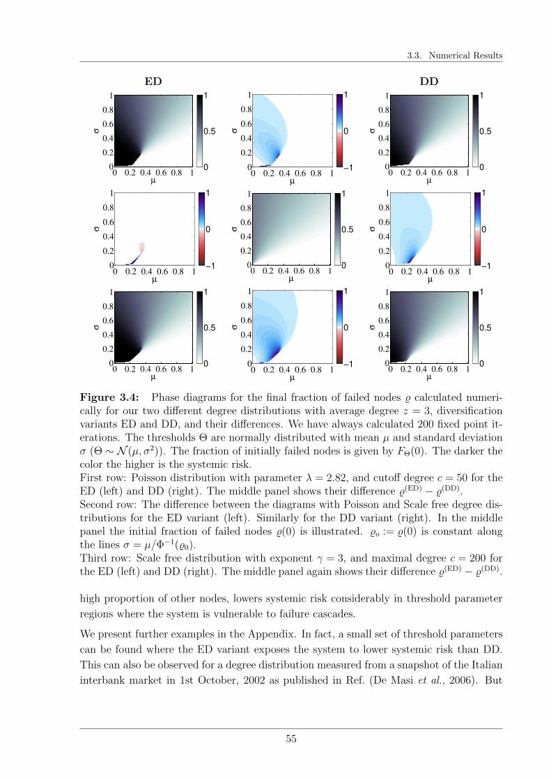
3.3. Numerical Results
ED DD
µ
σ
0 0.2 0.4 0.6 0.8 10
0.2
0.4
0.6
0.8
1
0
0.5
1
µ
σ
0 0.2 0.4 0.6 0.8 10
0.2
0.4
0.6
0.8
1
−1
0
1
µ
σ
0 0.2 0.4 0.6 0.8 10
0.2
0.4
0.6
0.8
1
0
0.5
1
µ
σ
0 0.2 0.4 0.6 0.8 10
0.2
0.4
0.6
0.8
1
−1
0
1
µ
σ
0 0.2 0.4 0.6 0.8 10
0.2
0.4
0.6
0.8
1
0
0.5
1
µ
σ
0 0.2 0.4 0.6 0.8 10
0.2
0.4
0.6
0.8
1
−1
0
1
µ
σ
0 0.2 0.4 0.6 0.8 10
0.2
0.4
0.6
0.8
1
0
0.5
1
µ
σ
0 0.2 0.4 0.6 0.8 10
0.2
0.4
0.6
0.8
1
−1
0
1
µσ
0 0.2 0.4 0.6 0.8 10
0.2
0.4
0.6
0.8
1
0
0.5
1
Figure 3.4: Phase diagrams for the final fraction of failed nodes % calculated numeri-cally for our two different degree distributions with average degree z = 3, diversificationvariants ED and DD, and their differences. We have always calculated 200 fixed point it-erations. The thresholds Θ are normally distributed with mean µ and standard deviationσ (Θ ∼ N (µ, σ2)). The fraction of initially failed nodes is given by FΘ(0). The darker thecolor the higher is the systemic risk.First row: Poisson distribution with parameter λ = 2.82, and cutoff degree c = 50 for theED (left) and DD (right). The middle panel shows their difference %(ED) − %(DD).Second row: The difference between the diagrams with Poisson and Scale free degree dis-tributions for the ED variant (left). Similarly for the DD variant (right). In the middlepanel the initial fraction of failed nodes %(0) is illustrated. %o := %(0) is constant alongthe lines σ = µ/Φ−1(%0).Third row: Scale free distribution with exponent γ = 3, and maximal degree c = 200 forthe ED (left) and DD (right). The middle panel again shows their difference %(ED) − %(DD).
high proportion of other nodes, lowers systemic risk considerably in threshold parameter
regions where the system is vulnerable to failure cascades.
We present further examples in the Appendix. In fact, a small set of threshold parameters
can be found where the ED variant exposes the system to lower systemic risk than DD.
This can also be observed for a degree distribution measured from a snapshot of the Italian
interbank market in 1st October, 2002 as published in Ref. (De Masi et al., 2006). But
55

Chapter 3. Diversification strategies in Constant Load models
0.1
0.2
0.3
0.4
0.5
0 10 20 30 40 50µ
P(
s=1
| k )
0.00
0.25
0.50
0.75
1.00
3 6 9µ
P(
s=1
| k )
0.00
0.25
0.50
0.75
1.00
3 6 9µ
P(
s=1
| k )
(a) (b) (c)
Figure 3.5: (a) Conditional failure probability for ED and normally distributed thresh-olds with parameters (µ, σ) = (0.3, 0.2) with π = 0.2 (black triangles), (µ, σ) = (0.15, 0.01)with π = 0.1 (red x), and (µ, σ) = (0.7, 0.2) with π = 0.3 (light blue +). Here,π is chosen independent of a cascade process. (b) Conditional failure probability forED and normally distributed thresholds with parameters (µ, σ) = (0.27, 0.09) (blackcircles), (µ, σ) = (0.3, 0.3) (dark blue +), (µ, σ) = (0.34, 0.19) (light blue triangles),(µ, σ) = (0.7, 0.6) (red x), and π defined by cascade equilibrium. Lines indicate a scalefree distribution, while symbols correspond to Poisson random graphs. (c) As in (b), butfor DD and red x refers to parameters (µ, σ) = (0.5, 0.5). Nodes with degree k > 10 havea similar failure probability as a node with degree k = 10.
the DD variant shows lower systemic risk than ED for most parameters also in this case.
Additionally, we provide an example where the sudden regime shift in the phase diagram
vanishes. Scale free random graphs with very low average degree z show in general only
small systemic risk (that is even smaller for DD than ED).
The presented results demonstrate that not only the overall connectivity z and robustness
(represented by the threshold parameters) determine the final cascade size. Other topo-
logical system properties as the specific distributions of degrees and link weights wij have
risk reduction potential as well.
The interplay of hubs and leaves seems to have an important effect. To understand their
different roles in the cascade amplification, we study next the failure risk of nodes condi-
tional on their degree.
3.3.2 Mesoscopic perspective
Two quantities reveal the role of the nodes with a given degree k in a cascade process: (a)
their failure probability P(s = 1∣∣ k) and (b) the cascade amplification that their failure
triggers. We measure the second quantity (b) as the increase of the fraction of failed nodes
% as response to an increase of their failure probability P(snb = 1∣∣ k) as neighbor. Thus,
56
3.3. Numerical Results
we call the partial derivative
∂%
∂P(snb = 1∣∣ k)
cascade amplification by a node with degree k.
For the ED variant the conditional failure probability (a) does not depend explicitly on
the degree distribution and thus the diversification strategies of the other nodes. It is
determined only by the failure probability of a neighbor π, which indicates the state of
the system in the cascade, and the threshold distribution. Equation (3.7) and (3.8) give:
P(s = 1∣∣ k) =
k∑n=0
b(n, k, π)FΘ
(nk
).
We would expect that large degrees, and thus, high diversification decreases the failure
risk, since the failure of a high number of neighbors is less probable than the failure of
fewer neighbors. As shown in Fig. 3.5(a), this intuition applies only to cases of small risk
where the failure probability π of a neighbor is small. Here, π is chosen independently of
a cascade evolution. For a few parameters with small threshold standard deviation σ, also
more irregular shapes of the conditional failure probability are possible (see, e.g., the red
circles in Fig. 3.5(a)). Still, in a real cascade process, the cascade keeps on-going in those
cases until most nodes are failed. Results of real ED cascade processes are depicted in
Fig. 3.5(b), where π is calculated in a fixed point iteration corresponding to the studied
threshold distribution. In this case, hubs have a higher risk to fail in a cascade than leaves
for almost all threshold parameters. Exceptions occur, e.g., (µ, σ) = (0.7, 0.6), but then
the difference in failure risk between hubs and leaves is negligible. Initially, hubs often
have a smaller failure risk than leaves. But if cascades get amplified and π increases, hubs
face a larger failure risk than leaves. High diversification becomes unfavorable. Intuitively,
nodes with a higher degree are more exposed to an ongoing cascade, as they have a higher
chance to be hit by it. But the diversification effect most often saturates for degrees
k > 10. Because of this we restrict Fig. 3.5(a) to k ≤ 10. The failure probability of a node
with degree k = 10 differs only marginally from the one of a node with higher degree.
This explains why we observe similar phase diagrams for Poisson and scale free random
graphs for the ED variant. The ED variant responds barely to changes in the tail of a
degree distribution, as nodes with large degrees have almost identical failure risk.
In contrast, for the DD variant, the outcome % depends crucially on the degree distribution.
Still, hubs have a higher failure risk than nodes with a smaller degree in general, see
Fig. 3.5(c). Each additional neighbor introduces the possibility of a loss, if it fails. Thus
57
Chapter 3. Diversification strategies in Constant Load models
the shape of the conditional failure probability
P(s = 1∣∣ k) = P
(Θ ≤
k∑j=0
(LnbDD
)j
)
always looks similar as the ones presented in Fig. 3.5(c). Consequently, too many nodes
with high degrees could increase the vulnerability of the system.
However, the presence of a few hubs also decreases the overall failure risk by decreasing
some of the possible losses. We gain this insight by studying the second indicator (b) that
describes the role of nodes in the cascade amplification. For both variants, ED and DD,
the partial derivative of % is of the form:
∂%
∂P(snb = 1∣∣ k)
= p(k)k[CED/DD − π
]. (3.10)
The constant CED/DD can be interpreted as failure probability of a neighbor where one
of its neighbors is failed and has degree k. Thus, the infinitesimal change in % is in fact
proportional to the increase of the failure probability of a neighbor.
In case of the ED variant, the constant CED does not depend on the degree k of a node
whose failure probability has increased:
CED =∑d
p(d)d
z
d−1∑n=0
b(n, d− 1, π)FΘ
(n+ 1
d
).
Consequently, the failure of hubs is especially problematic, as the cascade amplification is
proportional to the degree k of a failed node. The only way to reduce systemic risk (while
preserving the average degree z) in comparison to regular random graphs is to introduce
nodes to the system with smaller degree than z. Then, only a small fraction of hubs needs
to exist in order to preserve the average degree z. But the risk reduction is obtained by
the high number of small degree nodes.
In case of the DD variant, risk reduction is also obtained by the existence of hubs. The
constant CDD decreases with degree k:
CDD =∑d
p(d)d
zP
(Θ ≤ 1
k+
d−1∑j=0
(LnbDD
)j
).
The cascade amplification (Equation (3.10)) role of a node is decided by the trade-off
between the increasing factor p(k)k and the decreasing factor CDD − π. Especially less
diversified nodes (which have a chance to survive also large failure cascades) can benefit
from the diversification of others.
58

3.4. Discussion
3.4 Discussion
Although risk diversification is generally considered to lower the risk of an individual node,
on the system level it can even lead to the amplification of failures. With our work, we
have deepened the understanding of cascading failure processes in several ways.
At first, we generalize the method to calculate the systemic risk measure, i.e. the av-
erage cascade size, to include directed and weighted interactions. The loss that a node
experiences because of the failure of a neighbor can depend now also on properties of the
neighbor and not only on properties of the node itself. Moreover, we can correctly cal-
culate the time evolution of the cascade size, not only the final steady state. This allows
the analytic analysis of more complicated models. For instance, interventions in time as
response to an ongoing cascade could be tested and further questions answered as, e.g,
how the cascade can be blocked or further damage reduced.
The final cascade size as macro measure is complemented by a measure on the meso level,
by calculating individual failure probabilities of nodes based on their degree (diversifica-
tion).
This allows us to compare two different diversification mechanisms: ED (exposure diver-
sification) and DD (damage diversification). As we demonstrate, nodes which diversify
their exposures well (i.e. hubs), have a lower failure risk only as long as the system as
a whole is relatively robust. But above a certain threshold for the failure probability of
neighboring nodes, such hubs are at higher risk than other nodes because they are more
exposed to cascading failures. This effect tends to saturate for large degrees.
In general, most regulatory efforts follow the too big to fail strategy, and focus on the
prevention of the failures of systemic relevant nodes - the hubs. This is mainly achieved
by an increase of the thresholds, e.g. capital buffers in a financial context or immunization
in case of epidemic spreading. However, in reality this is often very costly.
With our study of another diversification strategy, the damage diversification, we suggest
to accompany regulatory efforts by mitigating the failure of hubs. By limiting the loss
that every node can impose on others, the damage potential of hubs and, thus, the over-
all systemic risk is significantly reduced. While this is systemically preferable, the DD
strategy is a two-edged sword: Hubs face an increased failure risk, but many small degree
nodes benefit from the diversification of their neighbors. This lowers the incentives for
diversification as long as no other benefit, e.g., higher gains in times of normal system
operation, comes along with a high degree.
As we show, the systemic relevance of a node is not solely defined by its degree, or con-
nectivity. The size of its impact in case of its failure, and thus its ability to cause further
failures is crucial. It is a strength of our approach that we can calculate this impact ana-
lytically and obtain a more refined and realistic identification of system relevant nodes. A
59

Chapter 3. Diversification strategies in Constant Load models
possible indicator for system relevance is the cascade amplification measure that we have
derived.
Additionally, our approach can be transfered to degree-degree correlated networks (Dodds
and Payne, 2009; Payne et al., 2009). We would expect that a high degree assortativity in
the DD could further reduce systemic risk, since the failure risk of diversified nodes could
be reduced by connections to hubs whose failures would impact their neighborhood only
little.
With our work we have given one example for systemic risk reduction by topological means.
Further possibilities can be explored with the analytical framework that we have provided.
60
Chapter 4
Correlations in Constant Load
models: Potential to reduce systemic
risk
Summary
We revisit the Constant Load Exposure and Damage Diversification modelvariants and study the impact of correlations between threshold and degreedistribution on systemic risk with the help of a Local Tree Approximation.This way, we explore an additional dimension to reduce systemic risk withoutchanging system performance or requiring additional resources. Along theway, we gain a deeper understanding of the role of well and less diversifiednodes in the evolution of a cascade. We test two extreme scenarios where thethreshold and degree distribution are perfectly correlated (pf) or perfectly anti-correlated (cf). Both variants have advantages in different parameter regionswhere a system could operate. This poses a system design question that isnot discussed or decisively answered by systemic risk researchers and policymakers. Is the goal to minimize the risk of large cascades or to avoid as manymediocre cascades as possible? And who has a higher priority in the allocationof limited resources - hubs or leaves? Or is there no preference?
This Chapter has been written specifically for this thesis. RB contributed to the design of the researchquestions, performed the analytic derivations, implemented the code and interpreted the results.
61
Chapter 4. Correlations in Constant Load models: Potential to reduce systemic risk
4.1 Introduction
According to Gigerenzer et al. (1999) and Gigerenzer (2015), good decisions in an uncertain
world often rely on simple rules that acknowledge the fact that a lot of information about
a problem at hand is not available. So called rules of thumb lead to good solutions many
times, although they require little time and knowledge.
Especially in complex systems, simplifications are crucial to guide decision and policy mak-
ers. In principle, system design decisions can have significant and surprising effects in the
presence of sudden regime shifts and phase transitions. These effects can be unexpectedly
positive, but also devastating. Because of this, care needs to be taken to regard enough
information about the ongoing processes. As we show, one rule might be very successful
in one setting, but a bad choice in another.
In this chapter, we test two simple rules of thumb for their effect on systemic risk in case
of Constant Load models (see Sec. 2.3.1). Both have been introduced already in Sec. 2.4.3
and concern the allocation of thresholds to nodes. Peripheral failures (pf) refer to a case
where nodes with higher degrees also receive higher thresholds, while in the opposite case,
central failures (cf), nodes with high degree are equipped with lower thresholds.
For instance, policy discussions about financial systemic risk tend to focus on the former,
pf. Primarily, large well connected institutions with big exposures are seen as system-
ically relevant (Arinaminpathy et al., 2012; Roukny et al., 2013) so that higher capital
requirements for these banks suggest a systemic risk reduction (Prasanna et al., 2011). In
reality, a situation similar to cf is observed by Arinaminpathy et al. (2012). Thus, large
institutions have lower relative capital buffers. Another example corresponds to epidemic
spreading, where the immunization of hubs seems to be effective (Pastor-Satorras and
Vespignani, 2002), again a pf strategy.
A pf threshold allocation is reasonable in models where primarily the failures of hubs
tend to amplify cascade processes. As we have discussed in the previous chapter, pf
should therefore reduce systemic for the CL ED model. But if the failure of hubs harms
the overall system only little, it is worth considering a cf allocation. Still, we find this
reasoning not to hold true for all parameters. A direct comparison between the most
promising combinations, ED and pf compared with DD and cf, poses a system design
question. While the former leads to negligible systemic risk for most threshold parameters,
the latter reduces the risk in regions where relatively big cascades occur. Presented with
these two options, assuming that the threshold parameters are out of control, the question
that decision makers would need to answer is: Do they prefer a relatively small risk of
large cascades that lead to an almost complete system break down or do they prefer to
reduce the size of these large cascades while accepting a higher risk of their occurrence at
the same time?
62
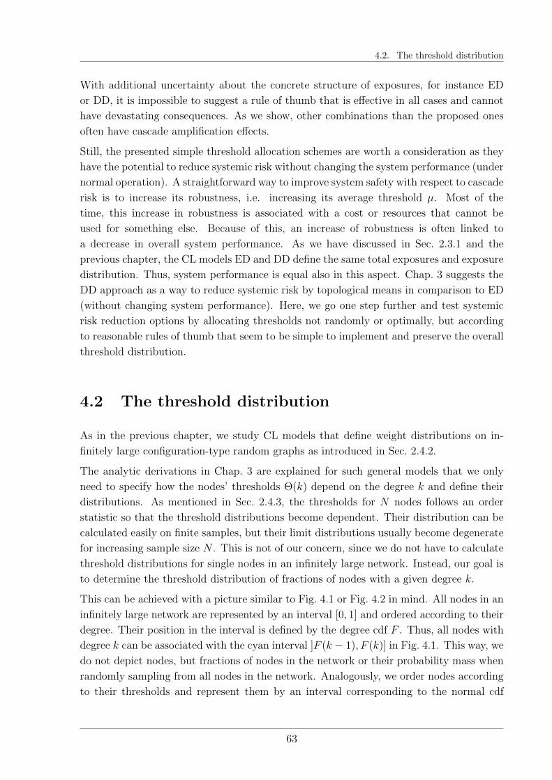
4.2. The threshold distribution
With additional uncertainty about the concrete structure of exposures, for instance ED
or DD, it is impossible to suggest a rule of thumb that is effective in all cases and cannot
have devastating consequences. As we show, other combinations than the proposed ones
often have cascade amplification effects.
Still, the presented simple threshold allocation schemes are worth a consideration as they
have the potential to reduce systemic risk without changing the system performance (under
normal operation). A straightforward way to improve system safety with respect to cascade
risk is to increase its robustness, i.e. increasing its average threshold µ. Most of the
time, this increase in robustness is associated with a cost or resources that cannot be
used for something else. Because of this, an increase of robustness is often linked to
a decrease in overall system performance. As we have discussed in Sec. 2.3.1 and the
previous chapter, the CL models ED and DD define the same total exposures and exposure
distribution. Thus, system performance is equal also in this aspect. Chap. 3 suggests the
DD approach as a way to reduce systemic risk by topological means in comparison to ED
(without changing system performance). Here, we go one step further and test systemic
risk reduction options by allocating thresholds not randomly or optimally, but according
to reasonable rules of thumb that seem to be simple to implement and preserve the overall
threshold distribution.
4.2 The threshold distribution
As in the previous chapter, we study CL models that define weight distributions on in-
finitely large configuration-type random graphs as introduced in Sec. 2.4.2.
The analytic derivations in Chap. 3 are explained for such general models that we only
need to specify how the nodes’ thresholds Θ(k) depend on the degree k and define their
distributions. As mentioned in Sec. 2.4.3, the thresholds for N nodes follows an order
statistic so that the threshold distributions become dependent. Their distribution can be
calculated easily on finite samples, but their limit distributions usually become degenerate
for increasing sample size N . This is not of our concern, since we do not have to calculate
threshold distributions for single nodes in an infinitely large network. Instead, our goal is
to determine the threshold distribution of fractions of nodes with a given degree k.
This can be achieved with a picture similar to Fig. 4.1 or Fig. 4.2 in mind. All nodes in an
infinitely large network are represented by an interval [0, 1] and ordered according to their
degree. Their position in the interval is defined by the degree cdf F . Thus, all nodes with
degree k can be associated with the cyan interval ]F (k − 1), F (k)] in Fig. 4.1. This way, we
do not depict nodes, but fractions of nodes in the network or their probability mass when
randomly sampling from all nodes in the network. Analogously, we order nodes according
to their thresholds and represent them by an interval corresponding to the normal cdf
63
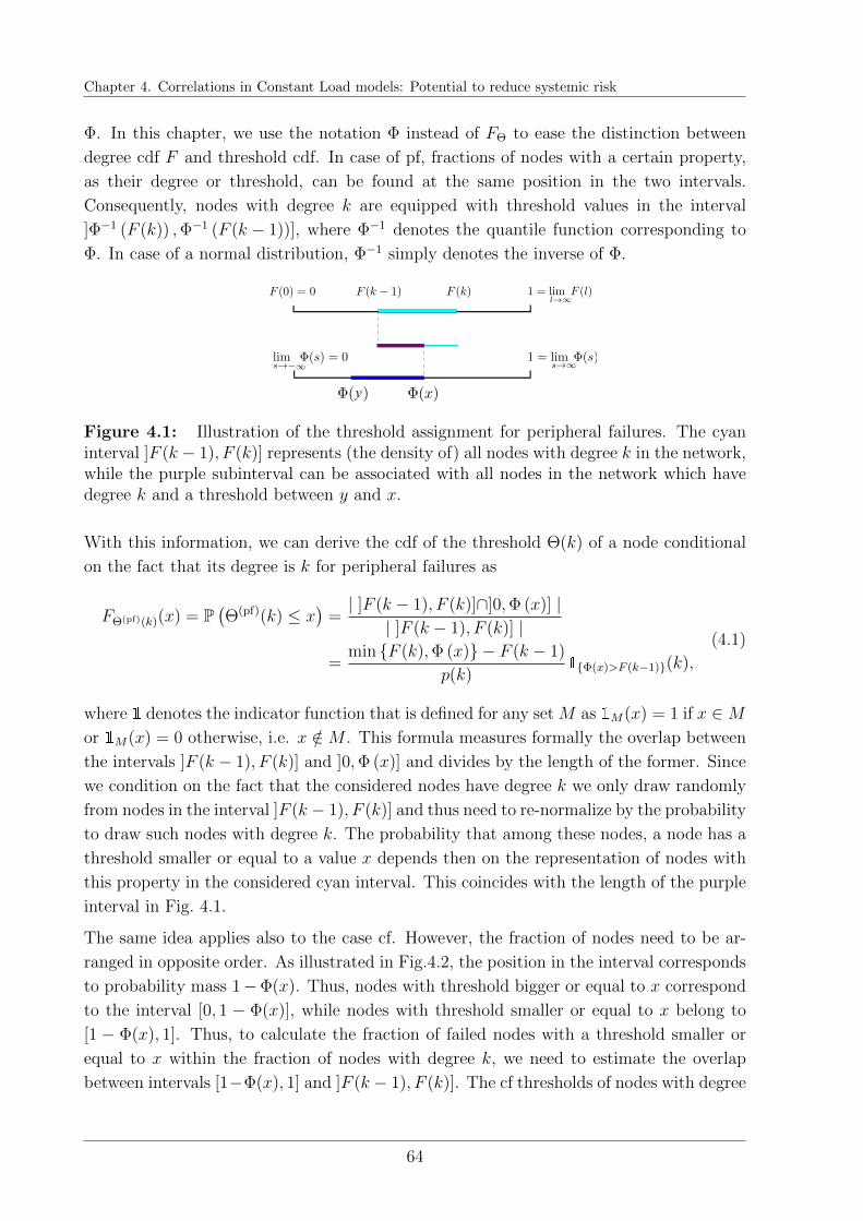
Chapter 4. Correlations in Constant Load models: Potential to reduce systemic risk
Φ. In this chapter, we use the notation Φ instead of FΘ to ease the distinction between
degree cdf F and threshold cdf. In case of pf, fractions of nodes with a certain property,
as their degree or threshold, can be found at the same position in the two intervals.
Consequently, nodes with degree k are equipped with threshold values in the interval
]Φ−1 (F (k)) ,Φ−1 (F (k − 1))], where Φ−1 denotes the quantile function corresponding to
Φ. In case of a normal distribution, Φ−1 simply denotes the inverse of Φ.
Figure 4.1: Illustration of the threshold assignment for peripheral failures. The cyaninterval ]F (k − 1), F (k)] represents (the density of) all nodes with degree k in the network,while the purple subinterval can be associated with all nodes in the network which havedegree k and a threshold between y and x.
With this information, we can derive the cdf of the threshold Θ(k) of a node conditional
on the fact that its degree is k for peripheral failures as
FΘ(pf)(k)(x) = P(Θ(pf)(k) ≤ x
)=| ]F (k − 1), F (k)]∩]0,Φ (x)] |
| ]F (k − 1), F (k)] |
=min F (k),Φ (x) − F (k − 1)
p(k)1Φ(x)>F (k−1)(k),
(4.1)
where 1 denotes the indicator function that is defined for any set M as 1M(x) = 1 if x ∈Mor 1M(x) = 0 otherwise, i.e. x /∈M . This formula measures formally the overlap between
the intervals ]F (k − 1), F (k)] and ]0,Φ (x)] and divides by the length of the former. Since
we condition on the fact that the considered nodes have degree k we only draw randomly
from nodes in the interval ]F (k − 1), F (k)] and thus need to re-normalize by the probability
to draw such nodes with degree k. The probability that among these nodes, a node has a
threshold smaller or equal to a value x depends then on the representation of nodes with
this property in the considered cyan interval. This coincides with the length of the purple
interval in Fig. 4.1.
The same idea applies also to the case cf. However, the fraction of nodes need to be ar-
ranged in opposite order. As illustrated in Fig.4.2, the position in the interval corresponds
to probability mass 1−Φ(x). Thus, nodes with threshold bigger or equal to x correspond
to the interval [0, 1 − Φ(x)], while nodes with threshold smaller or equal to x belong to
[1 − Φ(x), 1]. Thus, to calculate the fraction of failed nodes with a threshold smaller or
equal to x within the fraction of nodes with degree k, we need to estimate the overlap
between intervals [1−Φ(x), 1] and ]F (k − 1), F (k)]. The cf thresholds of nodes with degree
64

4.3. Cascade results
Figure 4.2: Illustration of the threshold assignment in case of central failures. The cyaninterval ]F (k − 1), F (k)] represents (the density of) all nodes with degree k in the network,while the purple subinterval can be associated with all nodes in the network which havedegree k and a threshold between y and x. In contrast to peripheral failures, nodes witha bigger threshold can be found on the left (and not on the right) of the unit interval.
k follow the distribution:
FΘ(cf)(k)(x) = P(Θ(cf)µ,σ (k) ≤ x
)=| ]F (k − 1), F (k)]∩]1− Φ (x) , 1] |
| ]F (k − 1), F (k)] |
=F (k)−max F (k − 1), 1− Φ (x)
p(k)1F (k)>1−Φ(x)(k).
(4.2)
With this choice of threshold distributions, we can calculate the fraction of failed nodes
by an LTA as explained in Chap. 3. Fig. 4.3 shows the perfect agreement of our numerical
calculations with simulations.
4.3 Cascade results
We give an overview about all possible combinations of ED and DD model variants with
pf and cf threshold allocation schemes in Fig. 4.4. Again, we present results for Poisson
and scale free degree distributions with the same average degree z = 3 as introduced in
Sec. 2.4.2.
We clearly find our intuition confirmed that pf in combination with ED reduces systemic
risk tremendously. This effect is even stronger for scale free networks in comparison to
Poisson random graphs. This is surprising to some extent, as the presence of a higher
fraction of hubs could mean that not all of them can be protected by high thresholds and
their failure could still amplify large cascades. But the high diversification also seems to
additionally reduce their failure risk. In Poisson random graphs, nodes with thresholds that
would survive cascades in a scale free network because of their large degree, can still fail
because enough of their smaller number of neighbors can trigger their failure. We account
the irregular shape of the phase diagrams corresponding to ED and DD noticeable. Our
65
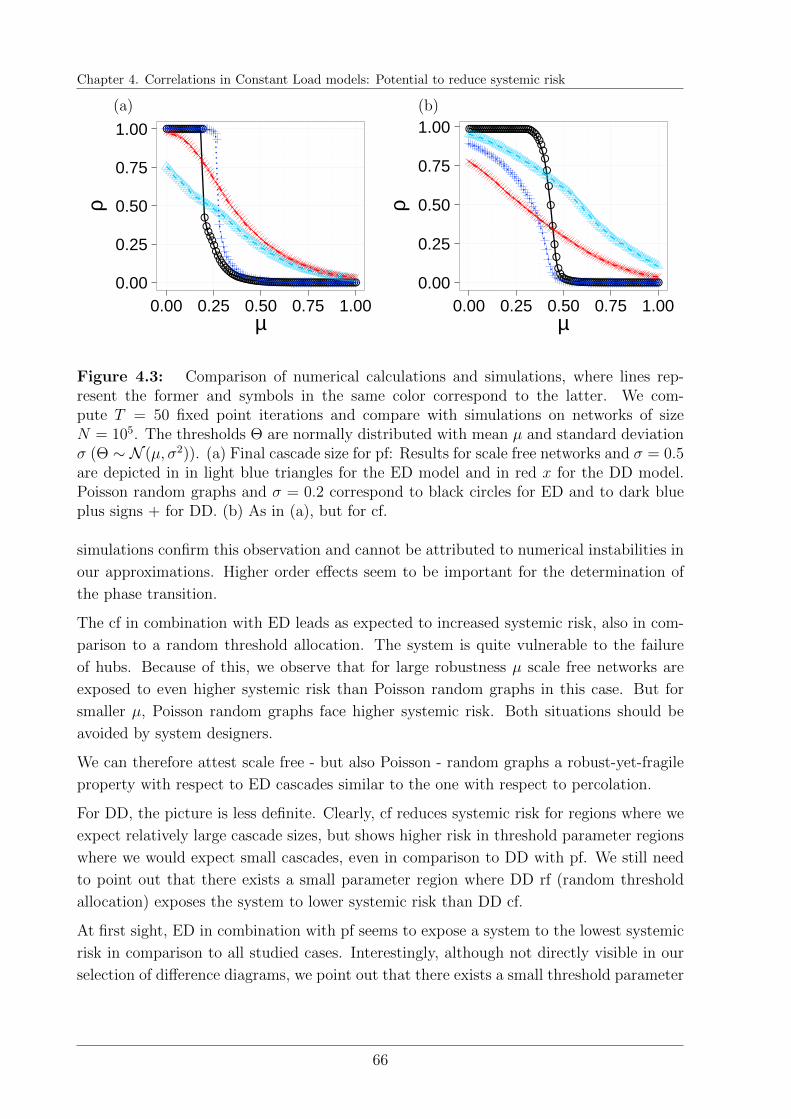
Chapter 4. Correlations in Constant Load models: Potential to reduce systemic risk
0.00
0.25
0.50
0.75
1.00
0.00 0.25 0.50 0.75 1.00µ
ρ
0.00
0.25
0.50
0.75
1.00
0.00 0.25 0.50 0.75 1.00µ
ρ
(a) (b)
Figure 4.3: Comparison of numerical calculations and simulations, where lines rep-resent the former and symbols in the same color correspond to the latter. We com-pute T = 50 fixed point iterations and compare with simulations on networks of sizeN = 105. The thresholds Θ are normally distributed with mean µ and standard deviationσ (Θ ∼ N (µ, σ2)). (a) Final cascade size for pf: Results for scale free networks and σ = 0.5are depicted in in light blue triangles for the ED model and in red x for the DD model.Poisson random graphs and σ = 0.2 correspond to black circles for ED and to dark blueplus signs + for DD. (b) As in (a), but for cf.
simulations confirm this observation and cannot be attributed to numerical instabilities in
our approximations. Higher order effects seem to be important for the determination of
the phase transition.
The cf in combination with ED leads as expected to increased systemic risk, also in com-
parison to a random threshold allocation. The system is quite vulnerable to the failure
of hubs. Because of this, we observe that for large robustness µ scale free networks are
exposed to even higher systemic risk than Poisson random graphs in this case. But for
smaller µ, Poisson random graphs face higher systemic risk. Both situations should be
avoided by system designers.
We can therefore attest scale free - but also Poisson - random graphs a robust-yet-fragile
property with respect to ED cascades similar to the one with respect to percolation.
For DD, the picture is less definite. Clearly, cf reduces systemic risk for regions where we
expect relatively large cascade sizes, but shows higher risk in threshold parameter regions
where we would expect small cascades, even in comparison to DD with pf. We still need
to point out that there exists a small parameter region where DD rf (random threshold
allocation) exposes the system to lower systemic risk than DD cf.
At first sight, ED in combination with pf seems to expose a system to the lowest systemic
risk in comparison to all studied cases. Interestingly, although not directly visible in our
selection of difference diagrams, we point out that there exists a small threshold parameter
66
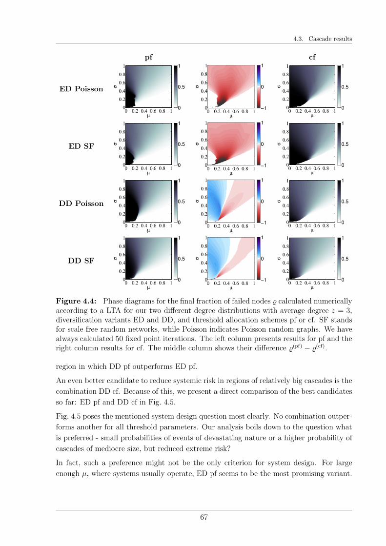
4.3. Cascade results
pf cf
ED Poisson
µσ
0 0.2 0.4 0.6 0.8 10
0.2
0.4
0.6
0.8
1
0
0.5
1
µ
σ
0 0.2 0.4 0.6 0.8 10
0.2
0.4
0.6
0.8
1
−1
0
1
µ
σ
0 0.2 0.4 0.6 0.8 10
0.2
0.4
0.6
0.8
1
0
0.5
1
ED SF
µ
σ
0 0.2 0.4 0.6 0.8 10
0.2
0.4
0.6
0.8
1
0
0.5
1
µ
σ
0 0.2 0.4 0.6 0.8 10
0.2
0.4
0.6
0.8
1
−1
0
1
µ
σ
0 0.2 0.4 0.6 0.8 10
0.2
0.4
0.6
0.8
1
0
0.5
1
DD Poisson
µ
σ
0 0.2 0.4 0.6 0.8 10
0.2
0.4
0.6
0.8
1
0
0.5
1
µ
σ
0 0.2 0.4 0.6 0.8 10
0.2
0.4
0.6
0.8
1
−1
0
1
µ
σ
0 0.2 0.4 0.6 0.8 10
0.2
0.4
0.6
0.8
1
0
0.5
1
DD SF
µ
σ
0 0.2 0.4 0.6 0.8 10
0.2
0.4
0.6
0.8
1
0
0.5
1
µ
σ
0 0.2 0.4 0.6 0.8 10
0.2
0.4
0.6
0.8
1
−1
0
1
µ
σ
0 0.2 0.4 0.6 0.8 10
0.2
0.4
0.6
0.8
1
0
0.5
1
Figure 4.4: Phase diagrams for the final fraction of failed nodes % calculated numericallyaccording to a LTA for our two different degree distributions with average degree z = 3,diversification variants ED and DD, and threshold allocation schemes pf or cf. SF standsfor scale free random networks, while Poisson indicates Poisson random graphs. We havealways calculated 50 fixed point iterations. The left column presents results for pf and theright column results for cf. The middle column shows their difference %(pf) − %(cf).
region in which DD pf outperforms ED pf.
An even better candidate to reduce systemic risk in regions of relatively big cascades is the
combination DD cf. Because of this, we present a direct comparison of the best candidates
so far: ED pf and DD cf in Fig. 4.5.
Fig. 4.5 poses the mentioned system design question most clearly. No combination outper-
forms another for all threshold parameters. Our analysis boils down to the question what
is preferred - small probabilities of events of devastating nature or a higher probability of
cascades of mediocre size, but reduced extreme risk?
In fact, such a preference might not be the only criterion for system design. For large
enough µ, where systems usually operate, ED pf seems to be the most promising variant.
67
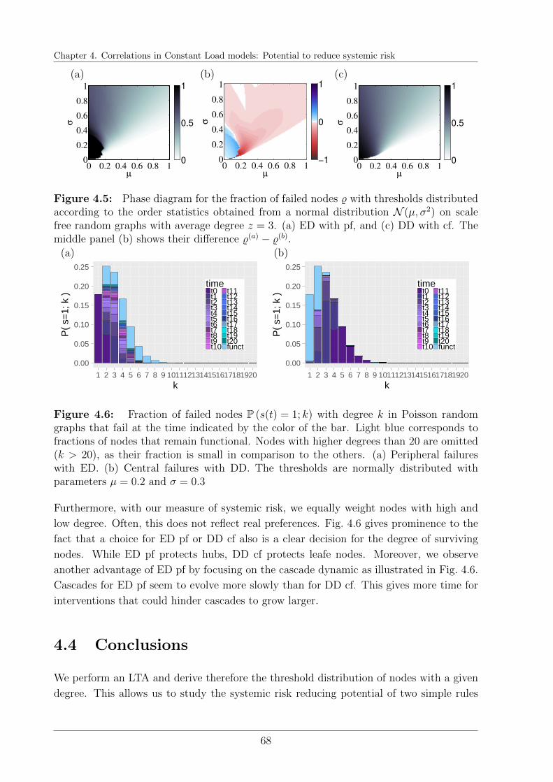
Chapter 4. Correlations in Constant Load models: Potential to reduce systemic risk
µ
σ
0 0.2 0.4 0.6 0.8 10
0.2
0.4
0.6
0.8
1
0
0.5
1
µ
σ
0 0.2 0.4 0.6 0.8 10
0.2
0.4
0.6
0.8
1
−1
0
1
µ
σ
0 0.2 0.4 0.6 0.8 10
0.2
0.4
0.6
0.8
1
0
0.5
1
(a) (b) (c)
Figure 4.5: Phase diagram for the fraction of failed nodes % with thresholds distributedaccording to the order statistics obtained from a normal distribution N (µ, σ2) on scalefree random graphs with average degree z = 3. (a) ED with pf, and (c) DD with cf. Themiddle panel (b) shows their difference %(a) − %(b).
0.00
0.05
0.10
0.15
0.20
0.25
1 2 3 4 5 6 7 8 9 1011121314151617181920k
P(
s=1;
k )
timet0t1t2t3t4t5t6t7t8t9t10
t11t12t13t14t15t16t17t18t19t20funct
0.00
0.05
0.10
0.15
0.20
0.25
1 2 3 4 5 6 7 8 9 1011121314151617181920k
P(
s=1;
k )
timet0t1t2t3t4t5t6t7t8t9t10
t11t12t13t14t15t16t17t18t19t20funct
(a) (b)
Figure 4.6: Fraction of failed nodes P (s(t) = 1; k) with degree k in Poisson randomgraphs that fail at the time indicated by the color of the bar. Light blue corresponds tofractions of nodes that remain functional. Nodes with higher degrees than 20 are omitted(k > 20), as their fraction is small in comparison to the others. (a) Peripheral failureswith ED. (b) Central failures with DD. The thresholds are normally distributed withparameters µ = 0.2 and σ = 0.3
Furthermore, with our measure of systemic risk, we equally weight nodes with high and
low degree. Often, this does not reflect real preferences. Fig. 4.6 gives prominence to the
fact that a choice for ED pf or DD cf also is a clear decision for the degree of surviving
nodes. While ED pf protects hubs, DD cf protects leafe nodes. Moreover, we observe
another advantage of ED pf by focusing on the cascade dynamic as illustrated in Fig. 4.6.
Cascades for ED pf seem to evolve more slowly than for DD cf. This gives more time for
interventions that could hinder cascades to grow larger.
4.4 Conclusions
We perform an LTA and derive therefore the threshold distribution of nodes with a given
degree. This allows us to study the systemic risk reducing potential of two simple rules
68

4.4. Conclusions
of thumb: One that allocates higher thresholds to well diversified nodes, i.e. nodes with
higher degree (pf), and one that allocates thresholds in opposite order, i.e. nodes with
higher degree receive a lower threshold (cf).
Both represent a way to reduce systemic risk without affecting system performance (un-
der normal system operation) or requiring additional resources. Neither is the dependence
structure nor the exposure distribution changed. Available thresholds are simply reallo-
cated according to the degree of nodes.
Both threshold allocation scenarios have different effects in combination with different
diversification strategies of nodes, the already discussed ED and DD CL cascade models.
Also both can lead to a cascade amplification in the wrong combination.
Lowest systemic risk can be achieved by ED pf and DD cf. While DD has proven to
outperform ED quite consistently under random threshold allocation, this picture has
changed for our correlation analysis. The region of high systemic in our phase diagrams is
smallest for ED pf. Moreover, cascades usually grow slower in time, which would give more
options for effective interventions that block large cascades. Finally, hubs have a higher
probability to withstand large cascades. Often hubs are more relevant to keep a system
functioning. DD cf clearly focuses on leaves instead of hubs in reducing their failure risk.
Even though the parameter region of mediocre cascades is larger, cascades are not of such
severe size as for ED pf. Thus, DD cf serves better policy makers or system designers with
high risk aversion.
Both combinations, ED pf and DD cf, have advantages and disadvantages that need to be
taken into account.
69

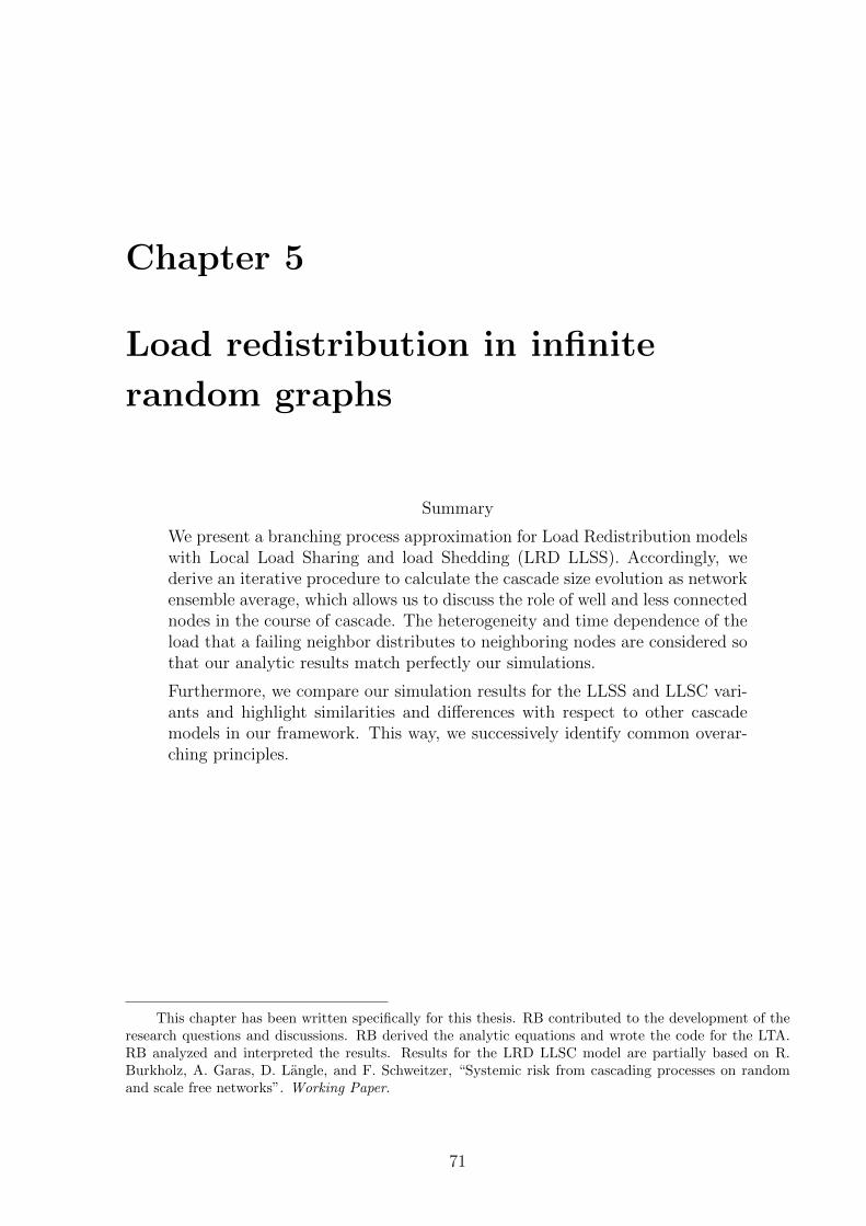
Chapter 5
Load redistribution in infinite
random graphs
Summary
We present a branching process approximation for Load Redistribution modelswith Local Load Sharing and load Shedding (LRD LLSS). Accordingly, wederive an iterative procedure to calculate the cascade size evolution as networkensemble average, which allows us to discuss the role of well and less connectednodes in the course of cascade. The heterogeneity and time dependence of theload that a failing neighbor distributes to neighboring nodes are considered sothat our analytic results match perfectly our simulations.
Furthermore, we compare our simulation results for the LLSS and LLSC vari-ants and highlight similarities and differences with respect to other cascademodels in our framework. This way, we successively identify common overar-ching principles.
This chapter has been written specifically for this thesis. RB contributed to the development of theresearch questions and discussions. RB derived the analytic equations and wrote the code for the LTA.RB analyzed and interpreted the results. Results for the LRD LLSC model are partially based on R.Burkholz, A. Garas, D. Langle, and F. Schweitzer, “Systemic risk from cascading processes on randomand scale free networks”. Working Paper.
71
Chapter 5. Load redistribution in infinite random graphs
5.1 Introduction
Fiber bundle models have become one of the most prevalent models to describe fracture
in materials (Sinha et al., 2015). Especially, the LRD LLSC model has been studied on
several topologies (Pradhan et al., 2010), in particular on random graphs that are similar
to our approach by Kim et al. (2005).
As discussed in Ch. 2, the network topology can be interpreted as dynamic in this case
and changes according to an evolving cascade. This creates a high path dependence of the
network structure on the precise steps of the cascade process and, even more problematic,
the clustering increases. This destroys the locally tree-like network structure on which an
LTA would rely on. Consequently, we cannot calculate the cascade size corresponding to
the LRD LLSC model analytically.
But, we can handle the LRD LLSS model. As we see in the following chapter, this is
already a non-trivial methodological extension of the existing (and also the so far pre-
sented) analytic description of cascade models. The additional challenge is introduced by
the variable load that a failing node distributes, because it also depends on the cascade
evolution and thus on the time of failure of the node. Thus, additional to the failure
probability of neighbors, we also need to keep track of the distribution of the load that a
neighbor distributes at a certain point in time before the failure of a node.
In future, it might be possible to tackle the LRD LLSC model by a combination of the
following work and an approach by Hackett and Gleeson (2013) to allow for non-zero
clustering in an LTA as well. But this goes beyond the scope of this thesis.
Accordingly, we mainly focus on the LRD LLSS model here. For a more in depth analysis
of the LRD LLSC model mainly by the means of simulations, we refer to Ref. (Kim
et al., 2005; Pradhan et al., 2010). Our own simulation results in Ch. 2 serve mainly
the comparison with the LRD LLSS model. We discuss briefly, why we observe increased
systemic risk for the LLSC case.
Next, we present our derivations for the analytic ensemble average of the cascade size for
the LLSS model and illustrate similarities with the CL DD model. In particular, our focus
lies on the role of hubs and leaves in the course of a cascade.
5.2 Local Tree Aproximation for the LRD model:
Local Load Sharing with load Shedding
In Sec. 2.6.1, we have provided the basis for the Local Tree Approximation of the LRD
LLSS model. To deduce the fraction of failed nodes %(t), we have to derive the distribution
of the load Lnb(k, t− 1) that a neighbor distributes at time t− 1 or before to a focal node
72
5.2. Local Tree Aproximation for the LRD model:Local Load Sharing with load Shedding
(or neighbor) with degree k.
As our following explanation is complicated enough, we restrict ourselves to the case of
the LRD LLSS model. A generalization to weighted networks is still straightforward
considering the following argumentation steps.
Recall that a focal neighbor with degree k accumulates a load
Λnb(k, t) =k−1∑j=1
Lnbj (k, t− 1)
over time. If it exceeds its threshold(Λnb(k, t) ≥ Θ(k)
)at time t the focal neighbor fails
and distributes exactly the load Λnb(k, t) to its nh functional network neighbors (including
the focal node under consideration). Thus, each functional neighbor receives the load
Λnb(k, t)/nh.
How does this relate to the load Lnbj (k, t− 1) that a neighbor spreads before or at time t?
Load distribution by a neighbor
First, we note that Λnb(k, t)/nh is independent of the degree of the load receiving focal
node or neighbor. The degree k belongs here to the failed neighbor. Consequently, we can
skip the degree dependence and write Lnbj (k, t− 1) = Lnbj (t− 1). In general, the load that
is distributed is influenced by the degree of the failing neighbor. But Lnbj (t−1) is the load
that is distributed by neighbor unconditional on the degree of this neighbor (thus without
the knowledge of its degree). The distribution of Lnbj (t− 1) incorporates the possibility of
a neighbor having different degrees.
Second, in contrast to our previous derivations for constant load models, the distributed
load is subject to the time t of a neighbor’s failure. Therefore, we need to ensure that we
respect the right order and time of failures. Only load that is distributed at time t can
trigger new failures at time t+ 1. Moreover, load is not distributed to neighbors that fail
at the same time.
To distinguish between failures before time t and at t, we introduce a new random variable,
the load ∆Lnb(t) that is distributed by a neighbor that fails exactly at time t and distributes
load at time t.
Let’s assume that we know the distribution of load Lnb(t− 1) by neighbors before time t.
We can then update Lnb(t− 1) to
pLnb(t)(l) = pLnb(t−1)(l) + p∆Lnb(t)(l), for all l ∈ R\0. (5.1)
Thus, we have reduced our problem to the derivation of the pdf corresponding to the load
73
Chapter 5. Load redistribution in infinite random graphs
∆Lnb(t) that is distributed at time t.
Load distribution at time t
Considering that we have two time steps in the history, failures at time t and t − 1, we
derive the updated load distribution at time t + 1. The distribution of ∆Lnb(t + 1) is
determined by several factors, i.e., the degree k of the failing focal neighbor, the number
no of neighbors of this focal neighbor that have failed at t− 1 before the failure could be
triggered, the number nn of newly failed neighbors at time t that distribute enough load
so that the threshold Θ(k) of the focal neighbor is exceeded and finally the number naof actual neighboring failures that do not receive load by the failing focal neighbor, since
they fail at the same time t+ 1.
Let’s assume the no old failed neighbors have distributed a load∑no
i=1 Lnbi (t−1) = lo before
or at time t, where each of the no neighbors has distributed a nonzero Lnbi (t− 1) > 0 load.
Additionally, the nn nodes distribute at time t the load∑nn
j=1 ∆Lnbj (t) = ln, where again
each of the nn neighbors has distributed a nonzero ∆Lnbj (t) > 0. We know that the
threshold Θ(k) of the focal neighbor under consideration must be bigger than lo + λ0 <
Θ(k). Otherwise, it would have had failed already. Moreover, ln + lo + λ0 ≥ Θ(k), since
the focal neighbor fails at time t. Under these assumptions, this neighbor distributes the
load
∆Lnb(t+ 1) =λ0 + lo + ln
k − no − nn − na=λ0 + lo + lnns + 1
to its remaining ns+1 functional network neighbors. ns = k−1−no−nn−na denotes here
the number of surviving neighbors that could also have failed before the focal neighbor.
With this observation, we simply need to sum up or integrate all possible probabilities
for the cases that lead to the distribution of a load l. This corresponds to a stepwise
application of Bayes’ Theorem that determines the state of the neighborhood of a focal
neighbor, i.e. the variables that influence the amount of load that is distributed.
The state of the neighborhood
We start with conditioning on the degree k of the focal neighbor and then proceed with
the different numbers of failed neighbors no, nn, na and the loads that they distribute (or
not distribute). First, we have for l > 0
P(∆Lnb(t+ 1) = l
)=
c∑k=1
p(k)k
zP(∆Lnb(t+ 1) = l
∣∣ Knb = k).
74
5.2. Local Tree Aproximation for the LRD model:Local Load Sharing with load Shedding
Next, we recall that we know already the distributions of Lnb(t−1) and ∆Lnb(t). Therefore,
we can calculate the pdf of Lnb(t) as well according to Eq. (5.1) and derive the probability
π(t+ 1) =c∑
k=1
p(k)k
zP
(Θ(k) ≤
k−1∑j=1
Lnbj (t)
)(5.2)
that a neighbor fails at time t+1 or before. Consequently, a neighbor of the focal neighbor
has failed with probability π(t) at time t or before, with probability π(t+ 1)− π(t) it fails
exactly at time t+ 1, and with probability 1− π(t+ 1) it is still functional at time t+ 1.
Because of the locally tree like network structure in the limit of infinite network size of
the configuration model, neighbors fail independently of each other. Thus, the random
variables (No, Nn, Na, Ns) that indicate the number of failed or non-failed neighbors at
specified times follow a multinomial distribution
(No, Nn, Na, Ns) ∼M (k − 1, π(t− 1), π(t)− π(t− 1), π(t+ 1)− π(t), 1− π(t+ 1)).
With Bayes’ Theorem we can further deduce:
P(∆Lnb(t+ 1) = l
)=
c∑k=1
p(k)k
z
k−1∑no=0
k−1−no∑nn=0
k−1−no−nn∑na=0
∫ ∞0
(k − 1)!
no!nn!na!ns!
× (1− π(t+ 1))ns (π(t+ 1)− π(t))na (π(t)− π(t− 1))nn πno(t− 1)
× P(∆Lnb(t+ 1) = l
∣∣ Knb = k,No = no, NN = nn, Na = na).
Instead of conditioning the load that is distributed on the failure of the corresponding
neighbors, we calculate directly the probability that a node fails and distributes a specific
nonzero load. Next, we consider thus the probabilities (π(t)− π(t− 1))nn and πno(t− 1)
already when counting all possible load distribution options that lead to a total load l that
is distributed to each of the ns + 1 remaining functional neighbors:
P(∆Lnb(t+ 1) = l
)=
=c∑
k=1
p(k)k
z
k−1∑no=0
k−1−no∑nn=0
k−1−no−nn∑na=0
∑x
(k − 1)!
no!nn!na!ns!(1− π(t+ 1))ns (π(t+ 1)− π(t))na
× P
(nn∑j=1
∆Lnbj (t) = x ; ∆Lnbj (t) > 0
)(FΘ(k) (l(ns + 1))− FΘ(k) (l(ns + 1)− x)
)× P
(no∑i=1
Lnbi (t− 1) = l(ns + 1)− λ0 − x ; Lnbi (t− 1) > 0
),
The sum runs over all discrete values x of the load distributed by failures at time t, since
for the LRD LLSS model the load distribution is discrete. We note that we have ln = x,
75
Chapter 5. Load redistribution in infinite random graphs
such that we obtain lo = l(ns + 1)− λ0 − x. Then, the load (ln + lo + λ0)/(ns + 1) = l is
newly distributed to a functional neighbor at time t+ 1. The probability
P (λ0 + lo ≤ Θ(k) ≤ λ0 + lo + ln) = FΘ(k) (l(ns + 1))− FΘ(k) (l(ns + 1)− x)
captures the case that the focal neighbor can withstand the load λnb(k, t) = lo + λ0, but
fails because of the load λnb(k, t+ 1) = ln + lo + λ0.
5.2.1 Cascade dynamics
In summary, we can describe the full cascade dynamics of the LRD LLSS model for
infinitely large configuration type random graphs (where the second moment of the degree
distribution is finite).
Initially, we start from the pdf of the load that is distributed by initially failing neighbors:
P(
∆Lnb(0) =λ0
ns + 1
)=
c∑k=ns+1
kp(k)
zFΘ(k)(λ0)b(k − 1− ns, k − 1, π(0))
for ns = 0, · · · , c− 1 and where π(0) is defined as
π(0) =c∑
k=1
p(k)k
zFΘ(k)(λ0). (5.3)
P(∆Lnb(0) = 0
)= 1− π(0) otherwise. Just formally, we define the pdf of the load that is
distributed by nodes before time t = 0 as zero:
P(Lnb(−1) = 0
)= 1.
On this basis, we can construct all following time steps iteratively.
At time t+ 1 we first determine the failure probability of a neighbor at time t+ 1 as:
π(t+ 1) =c∑
k=1
p(k)k
zP
(Θ(k) ≤
k−1∑j=1
Lnbj (t)
)
and compute next the distribution of load by a neighbor exactly at time t+ 1.
In the following no denotes the number of previously failed neighbors (before or at time
t− 1), nn the number of neighbors that have failed at time t, na the number of neighbors
that fail at time t+ 1 like the focal neighbor and ns the remaining functional neighbors of
the k − 1 possibly failing neighbors. FΘ(k) is the threshold distribution of a focal node or
76

5.3. Results
neighbor with degree k. We obtain:
P(∆Lnb(t+ 1) = l
)=
=c∑
k=1
p(k)k
z
k−1∑no=0
k−1−no∑nn=0
k−1−no−nn∑na=0
∑x
(k − 1)!
no!nn!na!ns!(1− π(t+ 1))ns (π(t+ 1)− π(t))na
× P
(nn∑j=1
∆Lnbj (t) = x ; ∆Lnbj (t) > 0
)(FΘ(k) (l(ns + 1))− FΘ(k) (l(ns + 1)− x)
)× P
(no∑i=1
Lnbi (t− 1) = l(ns + 1)− λ0 − x ; Lnbi (t− 1) > 0
),
for l > 0 and P(∆Lnb(t+ 1) = 0
)= 1− (π(t+ 1)− π(t)).
Then we update the pdf of the load Lnb(t− 1) that is distributed by a neighbor before or
at time t− 1 to Lnb(t) by
P(Lnb(t) = l
)= P
(Lnb(t− 1) = l
)+ P
(∆Lnb(t) = l
), for all l ∈ R\0
and P(Lnb(t) = 0
)= 1− π(t+ 1). Finally, with this definition, we determine the fraction
of failed nodes %(t+ 1) as:
%(t+ 1) =c∑
k=1
p(k)P
(Θ(k) ≤
k∑j=1
Lnbj (t)
)=
c∑k=1
p(k)∑x
FΘ(k)(x)p∗kLnb(t)(x). (5.4)
Despite the fact that the involved load distributions are discrete, we approximate the dis-
tributions on an equidistant grid in our numerical calculations. This allows us to compute
the convolutions of load distributions by Fast Fourier Transformation as in Chapt. 3 and
Chapt. 4. The general procedure is explained in Appendix A.2.
5.3 Results
We could repeat the same analysis as in the previous two chapters for the Constant
Load models. Conceptually, we only need to specify the threshold distribution, degree
distribution, and the initial load λ0.
In case of random failures, we assume that the thresholds follow a normal distribution
independent of the degree of a node, i.e. Θ ∼ N (µ+ λ0, σ2). We add λ0 to the mean
threshold value to ensure that nodes fail with the same initial probability as in all other
studied cases. With the same set of parameters, but otherwise as in Chapt. 4, we can
define the threshold distributions in case of correlations between threshold and degree
distribution.
77
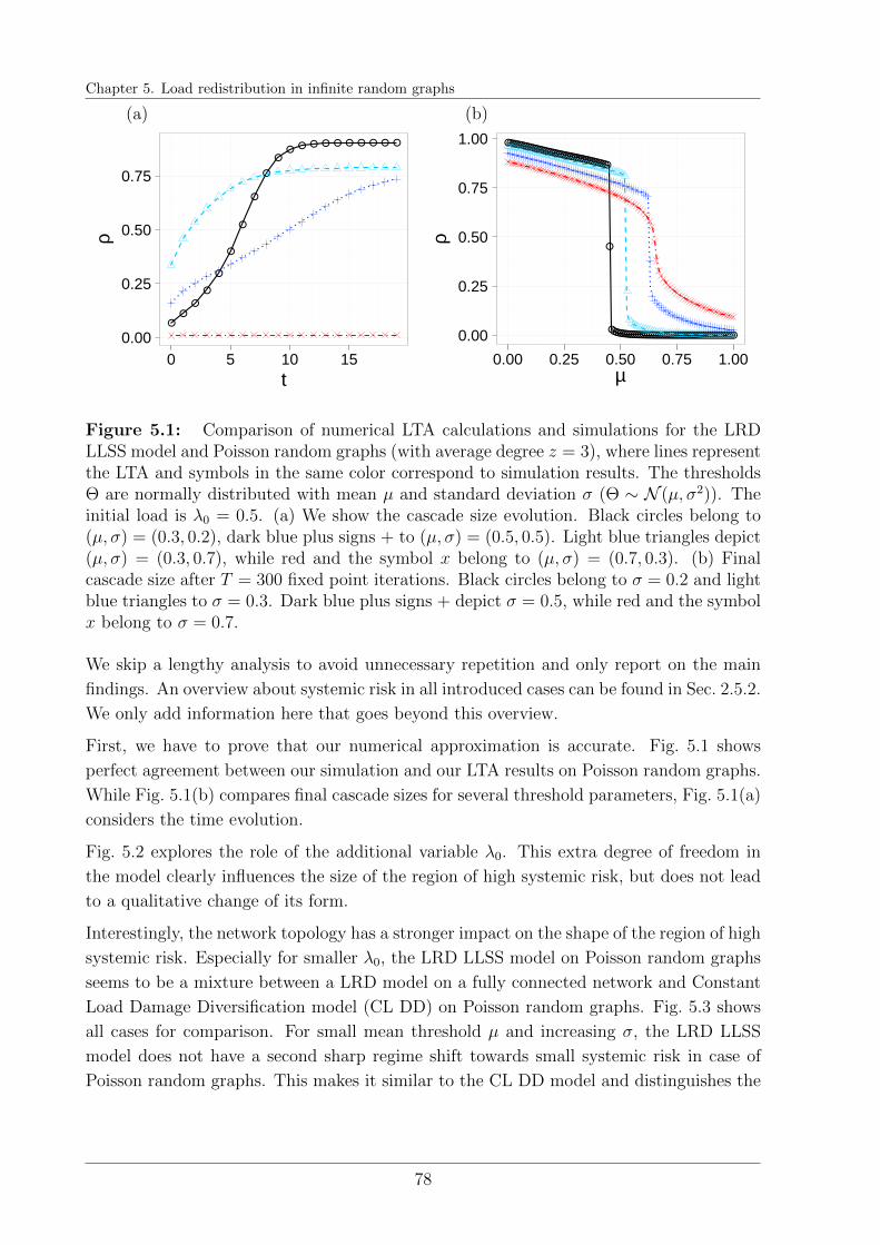
Chapter 5. Load redistribution in infinite random graphs
0.00
0.25
0.50
0.75
0 5 10 15t
ρ
0.00
0.25
0.50
0.75
1.00
0.00 0.25 0.50 0.75 1.00µ
ρ
(a) (b)
Figure 5.1: Comparison of numerical LTA calculations and simulations for the LRDLLSS model and Poisson random graphs (with average degree z = 3), where lines representthe LTA and symbols in the same color correspond to simulation results. The thresholdsΘ are normally distributed with mean µ and standard deviation σ (Θ ∼ N (µ, σ2)). Theinitial load is λ0 = 0.5. (a) We show the cascade size evolution. Black circles belong to(µ, σ) = (0.3, 0.2), dark blue plus signs + to (µ, σ) = (0.5, 0.5). Light blue triangles depict(µ, σ) = (0.3, 0.7), while red and the symbol x belong to (µ, σ) = (0.7, 0.3). (b) Finalcascade size after T = 300 fixed point iterations. Black circles belong to σ = 0.2 and lightblue triangles to σ = 0.3. Dark blue plus signs + depict σ = 0.5, while red and the symbolx belong to σ = 0.7.
We skip a lengthy analysis to avoid unnecessary repetition and only report on the main
findings. An overview about systemic risk in all introduced cases can be found in Sec. 2.5.2.
We only add information here that goes beyond this overview.
First, we have to prove that our numerical approximation is accurate. Fig. 5.1 shows
perfect agreement between our simulation and our LTA results on Poisson random graphs.
While Fig. 5.1(b) compares final cascade sizes for several threshold parameters, Fig. 5.1(a)
considers the time evolution.
Fig. 5.2 explores the role of the additional variable λ0. This extra degree of freedom in
the model clearly influences the size of the region of high systemic risk, but does not lead
to a qualitative change of its form.
Interestingly, the network topology has a stronger impact on the shape of the region of high
systemic risk. Especially for smaller λ0, the LRD LLSS model on Poisson random graphs
seems to be a mixture between a LRD model on a fully connected network and Constant
Load Damage Diversification model (CL DD) on Poisson random graphs. Fig. 5.3 shows
all cases for comparison. For small mean threshold µ and increasing σ, the LRD LLSS
model does not have a second sharp regime shift towards small systemic risk in case of
Poisson random graphs. This makes it similar to the CL DD model and distinguishes the
78
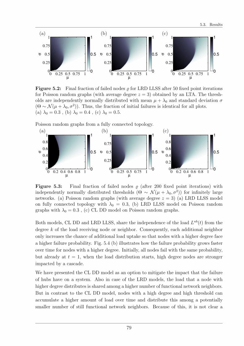
5.3. Results
µ
σ
0 0.25 0.5 0.75 10
0.25
0.5
0.75
1
0
0.5
1
µ
σ
0 0.25 0.5 0.75 10
0.25
0.5
0.75
1
0
0.5
1
µ
σ
0 0.25 0.5 0.75 10
0.25
0.5
0.75
1
0
0.5
1(a) (b) (c)
Figure 5.2: Final fraction of failed nodes % for LRD LLSS after 50 fixed point iterationsfor Poisson random graphs (with average degree z = 3) obtained by an LTA. The thresh-olds are independently normally distributed with mean µ + λ0 and standard deviation σ(Θ ∼ N (µ+ λ0, σ
2)). Thus, the fraction of initial failures is identical for all plots.(a) λ0 = 0.3 , (b) λ0 = 0.4 , (c) λ0 = 0.5.
Poisson random graphs from a fully connected topology.
µ
σ
0 0.2 0.4 0.6 0.8 10
0.2
0.4
0.6
0.8
1
0
0.5
1
µ
σ
0 0.25 0.5 0.75 10
0.25
0.5
0.75
1
0
0.5
1
µ
σ
0 0.2 0.4 0.6 0.8 10
0.2
0.4
0.6
0.8
1
0
0.5
1
(a) (b) (c)
Figure 5.3: Final fraction of failed nodes % (after 200 fixed point iterations) withindependently normally distributed thresholds (Θ ∼ N (µ + λ0, σ
2)) for infinitely largenetworks. (a) Poisson random graphs (with average degree z = 3) (a) LRD LLSS modelon fully connected topology with λ0 = 0.3, (b) LRD LLSS model on Poisson randomgraphs with λ0 = 0.3 , (c) CL DD model on Poisson random graphs.
Both models, CL DD and LRD LLSS, share the independence of the load Lnb(t) from the
degree k of the load receiving node or neighbor. Consequently, each additional neighbor
only increases the chance of additional load uptake so that nodes with a higher degree face
a higher failure probability. Fig. 5.4 (b) illustrates how the failure probability grows faster
over time for nodes with a higher degree. Initially, all nodes fail with the same probability,
but already at t = 1, when the load distribution starts, high degree nodes are stronger
impacted by a cascade.
We have presented the CL DD model as an option to mitigate the impact that the failure
of hubs have on a system. Also in case of the LRD models, the load that a node with
higher degree distributes is shared among a higher number of functional network neighbors.
But in contrast to the CL DD model, nodes with a high degree and high threshold can
accumulate a higher amount of load over time and distribute this among a potentially
smaller number of still functional network neighbors. Because of this, it is not clear a
79
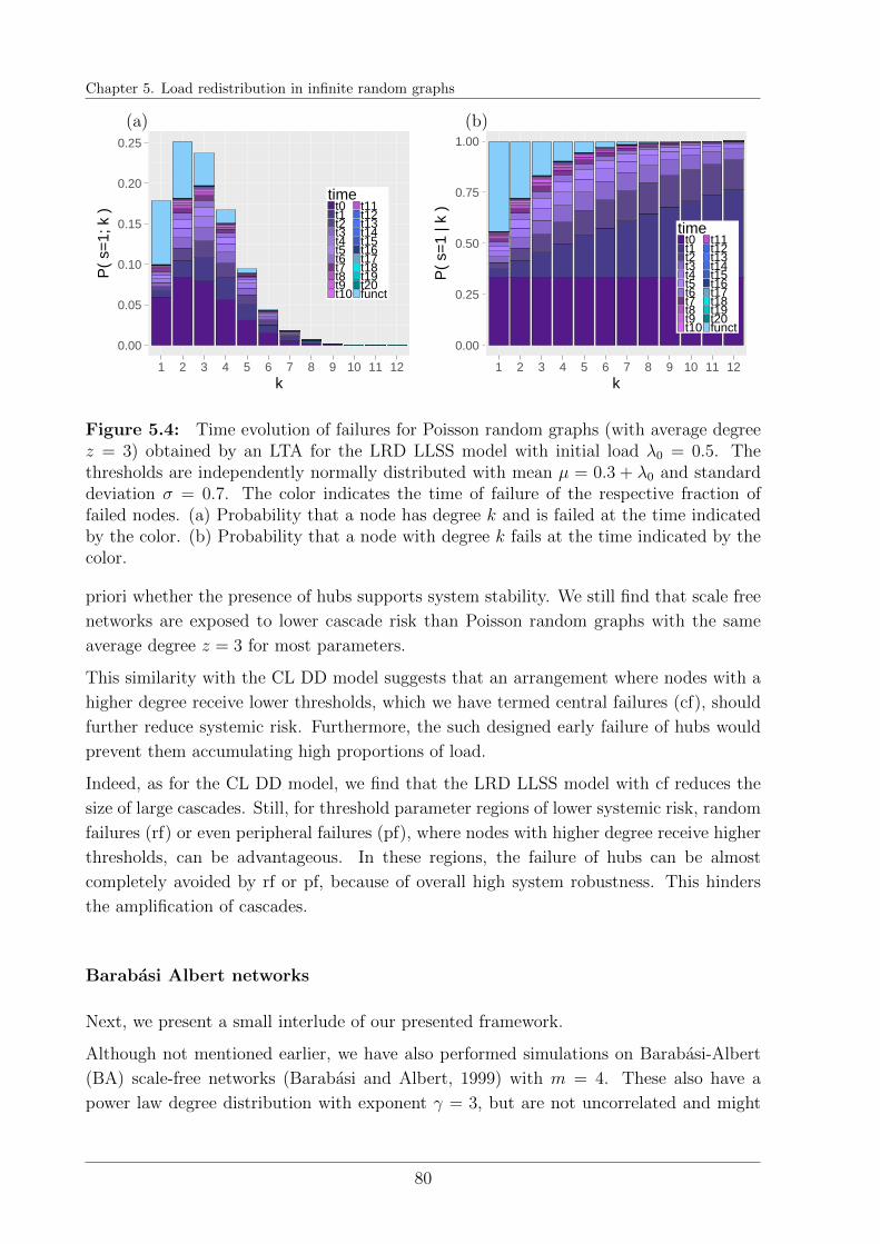
Chapter 5. Load redistribution in infinite random graphs
0.00
0.05
0.10
0.15
0.20
0.25
1 2 3 4 5 6 7 8 9 10 11 12k
P(
s=1;
k )
timet0t1t2t3t4t5t6t7t8t9t10
t11t12t13t14t15t16t17t18t19t20funct
0.00
0.25
0.50
0.75
1.00
1 2 3 4 5 6 7 8 9 10 11 12k
P(
s=1
| k )
timet0t1t2t3t4t5t6t7t8t9t10
t11t12t13t14t15t16t17t18t19t20funct
(a) (b)
Figure 5.4: Time evolution of failures for Poisson random graphs (with average degreez = 3) obtained by an LTA for the LRD LLSS model with initial load λ0 = 0.5. Thethresholds are independently normally distributed with mean µ = 0.3 + λ0 and standarddeviation σ = 0.7. The color indicates the time of failure of the respective fraction offailed nodes. (a) Probability that a node has degree k and is failed at the time indicatedby the color. (b) Probability that a node with degree k fails at the time indicated by thecolor.
priori whether the presence of hubs supports system stability. We still find that scale free
networks are exposed to lower cascade risk than Poisson random graphs with the same
average degree z = 3 for most parameters.
This similarity with the CL DD model suggests that an arrangement where nodes with a
higher degree receive lower thresholds, which we have termed central failures (cf), should
further reduce systemic risk. Furthermore, the such designed early failure of hubs would
prevent them accumulating high proportions of load.
Indeed, as for the CL DD model, we find that the LRD LLSS model with cf reduces the
size of large cascades. Still, for threshold parameter regions of lower systemic risk, random
failures (rf) or even peripheral failures (pf), where nodes with higher degree receive higher
thresholds, can be advantageous. In these regions, the failure of hubs can be almost
completely avoided by rf or pf, because of overall high system robustness. This hinders
the amplification of cascades.
Barabasi Albert networks
Next, we present a small interlude of our presented framework.
Although not mentioned earlier, we have also performed simulations on Barabasi-Albert
(BA) scale-free networks (Barabasi and Albert, 1999) with m = 4. These also have a
power law degree distribution with exponent γ = 3, but are not uncorrelated and might
80

5.4. Local Load Conservation in comparison
µ
σ
0 0.25 0.5 0.75 10
0.25
0.5
0.75
1
0
0.5
1
µ
σ
0 0.25 0.5 0.75 10
0.25
0.5
0.75
1
0
0.5
1
µ
σ
0 0.25 0.5 0.75 10
0.25
0.5
0.75
1
0
0.5
1(a) (b) (c)
Figure 5.5: Final fraction of failed nodes % for simulations of LRD LLSS cascadesas average over 100 independent realizations of BA networks consisting of N = 1000nodes. The thresholds are normally distributed with mean µ+ λ0 and standard deviationσ (Θ ∼ N (µ + λ0, σ
2)), where the initial load is λ0 = 0.4. We consider three differentthreshold allocations: (a) pf , (b) rf , (c) cf.
also have non-zero clustering, since we study networks of size N = 1000.
We present our results for the LLSS model, because they are noticeable and surprising. In
fact, this model has already been studied by Moreno et al. (2002) on BA networks. But
the thresholds have been independently distributed according to a Weibull distribution.
First and foremost, we are interested in the effect of correlations between threshold and
degree distribution.
Fig. 5.5 shows the average over 100 independent network realizations of the fraction of
failed nodes for normally distributed thresholds. Remarkably, the central failures threshold
allocation is extremely effective in the reduction of systemic risk. In no other case have we
encountered such a shape of the phase diagram and so small systemic risk for very small
mean threshold values µ.
How this can be explained needs to be investigated further, but goes beyond the framework
studied in this thesis. We hypothesize that the protection of a highly connected core
consisting of nodes with a high degree and thus also high threshold in the cf scheme
hampers cascades effectively.
5.4 Local Load Conservation in comparison
In Ch. 2, we have seen that the LRD LLSC model leads to higher cascade sizes than
the LRD LLSS model in general and have attributed this observation to the growing
interconnectivity of networks in case of LLSC, which introduces a high similarity with
cascades on fully connected networks (Kim et al., 2005).
This increasing connectivity creates nodes with large degrees, especially if hubs fail early
and all their functional neighbors become connected. Because of this, cf usually increases
systemic risk in comparison to rf or pf for LLSC in contrast to LLSS. For the initial load
81
Chapter 5. Load redistribution in infinite random graphs
size λ0 = 0.5, we cannot observe a high difference between different thresholds allocations
in Fig. 2.10. But for smaller initial loads, the explained difference becomes apparent.
A high connectivity amplifies failure cascades, if too high amounts of load are distributed.
If many nodes are already close to failure and they all are formed to a fully connected
clique, only a few of them need to be hit by the cascade, distribute their load and carry
the others down as well in the next step. Thus, the damage diversification effect by high
degree nodes is small in comparison to the increase of failure probability that a high degree
brings along.
With the OLRD model, where much smaller amounts of load are distributed, we observe
the opposite. There, the damage diversification effect by hubs seems to prevail their
increased failure probability, simply because most of the nodes of formed cliques are not
close to failure.
5.5 Conclusions
We have presented an LTA that correctly captures the time evolution of the LRD LLSS
model by analytic means. The most crucial innovation in comparison with the LTA for
CL models as presented in Ch. 3 is the iterative calculation of the load distribution by a
random neighbor that has failed before a given time t. In comparison with simulations,
our LTA approximation leads considerably faster to results than simulations and captures
accurately the cascade size on large networks, even if simulations become impossible in
this setting.
The correctness of time evolution might allow in future research to add process complexity
in time, for instance, similar as in the model for creep rupture (Danku et al., 2015; Halasz
et al., 2012; Kun et al., 2008, 2009) and still obtain an analytic description of the cascade
size.
We have noted that the load that a neighbor distributes is independent of the degree of
the receiving node in case of both studied models, the LLSS and LLSC variant. This
is a property that they share with the earlier discussed CL DD model. Consequently,
the larger the degree of the node the higher is its failure risk. Despite the high damage
diversification for the failure of hubs, an increasing connectivity of the networks (as in case
of LLSC model) tends to increase systemic risk, if enough initial load is distributed.
Still, without increasing connectivity in case of the LLSS model, the cf threshold allocation
reduces systemic risk remarkably, especially for BA random graphs. Cf leads to an early
failure of hubs and prevents thus a high accumulation of load over time until they fail.
Furthermore, it disconnects the system early on which lowers the opportunity for cascades
to propagate through the entire network.
82

5.5. Conclusions
On the contrary, the connectivity even increases in case of LLSC so that systemic risk is
usually higher for cf in comparison with rf and, in particular, pf.
We have attributed the difference between the LLSS and LLSC variants to a trade-off
between increasing failure risk for nodes with high degree and the systemic risk reducing
effect by a better damage diversification that is caused by the failure of nodes with a
higher degree.
In the next chapter, we revisit the OLRD model, where this trade-off is decided in the
opposite direction. There, LLSC leads to lower systemic risk than LLSS. Furthermore, we
extend our LTA to match OLRD type models.
83

Chapter 6
Overload redistribution in infinite
random graphs
Summary
Our main contribution in this chapter is our analytic branching process approx-imation of the cascade size evolution for the OLRD LLSS model. Furthermore,we compare cascade results of the OLRD and LRD model and explain why weobserve higher systemic risk for the LRD LLSC model compared with the LRDLLSS model, but observe the reverse effect for the OLRD counterparts. Thisobservation refers to a trade-off between increased exposure and increased dam-age diversification of well connected nodes. We hypothesize that this trade-offis of specific relevance in the early evolution of a cascade.
RB has written this chapter specifically for this thesis. RB contributed to discussions and thedevelopment of the research questions. RB derived the analytic equations and wrote the code for theLTA. RB analyzed and interpreted the results. Simulations are partially based on R. Burkholz, A. Garas,D. Langle, and F. Schweitzer, “Systemic risk from cascading processes on random and scale free networks”.Working Paper.
85

Chapter 6. Overload redistribution in infinite random graphs
6.1 Introduction
Neither the LLSC nor the LLSS model variants in our OLRD class have been studied on
configuration model type random graph ensembles up to our knowledge. Still, the aspect
of cascading overload failures is a widely observed phenomenon and it is a reasonable as-
sumption that a system has the capacity to absorb a certain amount of load. Or overloaded
components do not fail and keep still functioning, but process only a certain amount of
load while the remaining load is distributed to other nodes in the system. Often, this
redistribution of load follows more complicated procedures. For instance, it depends on
the betweenness of nodes in a network.This would require global information about the
network topology, which we cannot consider in a Local Tree Approximation (LTA).
Here, we focus on simplified model versions, where load is distributed locally and which
we can compare with their LRD counterparts. For the same reasons as in case of LRD, we
cannot describe the cascade size evolution of the LLSC model analytically. The increasing
clustering violates our assumption of a locally tree like network structure.
For the OLRD LLSS model, we derive an LTA and compare our results with our findings
for the LRD model.
6.2 Local Tree Approximation for the OLRD model:
Local Load Sharing with load Shedding
The Overload Redistribution Local Load Sharing with load Shedding model is similar to
its Load redistribution variant and so is its Local Tree Approximation. An additional
challenge is introduced by the fact that the load Lnb(t) that a neighbor distributes before
or at time t is not discrete, if the thresholds are continuously distributed. Because of
this, we deduce the cumulative distribution function of the load ∆Lnb(t) that a neighbor
distributes exactly at time t and Lnb(t) instead of its probability distribution function (or
density in this case).
Let’s assume a focal neighbor with degree k that fails at time t carries the load λnb(k, t),
which exceeds its threshold θ(k). With exactly ns + 1 functional network neighbors, the
focal neighbor distributes to each of them the load
λnb(k, t)− θ(k)
ns + 1=
∑ni=1 l
nbi (t− 1)
k − n,
if n of its network neighbors have failed before and have distributed a load lnbi (t− 1) and
the initial load λ0 is set to zero (λ0 = 0). As for the LRD model variant, this load does
not depend on properties of the receiving functional network neighbors. Consequently, the
86
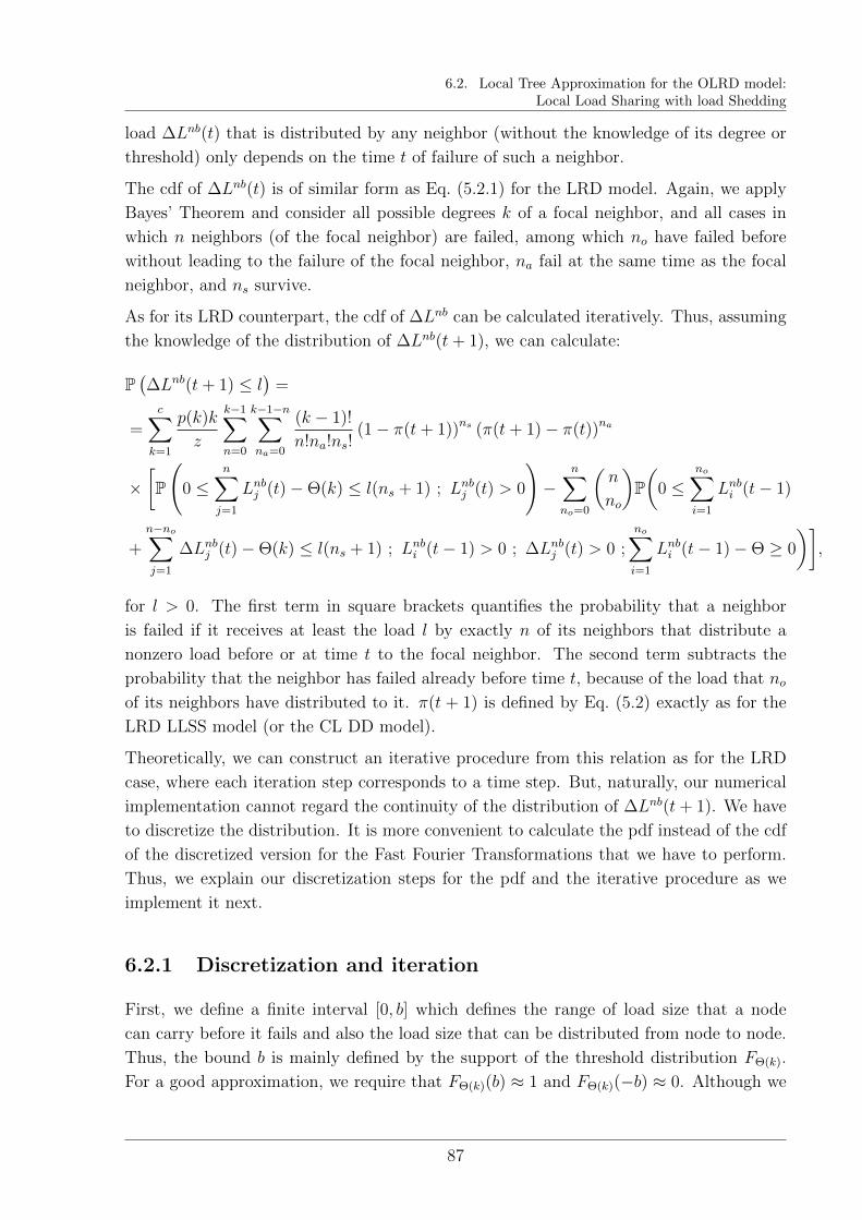
6.2. Local Tree Approximation for the OLRD model:Local Load Sharing with load Shedding
load ∆Lnb(t) that is distributed by any neighbor (without the knowledge of its degree or
threshold) only depends on the time t of failure of such a neighbor.
The cdf of ∆Lnb(t) is of similar form as Eq. (5.2.1) for the LRD model. Again, we apply
Bayes’ Theorem and consider all possible degrees k of a focal neighbor, and all cases in
which n neighbors (of the focal neighbor) are failed, among which no have failed before
without leading to the failure of the focal neighbor, na fail at the same time as the focal
neighbor, and ns survive.
As for its LRD counterpart, the cdf of ∆Lnb can be calculated iteratively. Thus, assuming
the knowledge of the distribution of ∆Lnb(t+ 1), we can calculate:
P(∆Lnb(t+ 1) ≤ l
)=
=c∑
k=1
p(k)k
z
k−1∑n=0
k−1−n∑na=0
(k − 1)!
n!na!ns!(1− π(t+ 1))ns (π(t+ 1)− π(t))na
×[P
(0 ≤
n∑j=1
Lnbj (t)−Θ(k) ≤ l(ns + 1) ; Lnbj (t) > 0
)−
n∑no=0
(n
no
)P(
0 ≤no∑i=1
Lnbi (t− 1)
+n−no∑j=1
∆Lnbj (t)−Θ(k) ≤ l(ns + 1) ; Lnbi (t− 1) > 0 ; ∆Lnbj (t) > 0 ;no∑i=1
Lnbi (t− 1)−Θ ≥ 0
)],
for l > 0. The first term in square brackets quantifies the probability that a neighbor
is failed if it receives at least the load l by exactly n of its neighbors that distribute a
nonzero load before or at time t to the focal neighbor. The second term subtracts the
probability that the neighbor has failed already before time t, because of the load that noof its neighbors have distributed to it. π(t + 1) is defined by Eq. (5.2) exactly as for the
LRD LLSS model (or the CL DD model).
Theoretically, we can construct an iterative procedure from this relation as for the LRD
case, where each iteration step corresponds to a time step. But, naturally, our numerical
implementation cannot regard the continuity of the distribution of ∆Lnb(t+ 1). We have
to discretize the distribution. It is more convenient to calculate the pdf instead of the cdf
of the discretized version for the Fast Fourier Transformations that we have to perform.
Thus, we explain our discretization steps for the pdf and the iterative procedure as we
implement it next.
6.2.1 Discretization and iteration
First, we define a finite interval [0, b] which defines the range of load size that a node
can carry before it fails and also the load size that can be distributed from node to node.
Thus, the bound b is mainly defined by the support of the threshold distribution FΘ(k).
For a good approximation, we require that FΘ(k)(b) ≈ 1 and FΘ(k)(−b) ≈ 0. Although we
87

Chapter 6. Overload redistribution in infinite random graphs
later on consider normal distributions, which have theoretically support R, numerically,
the choice b = 5 satisfies our requirements for all considered parameters.
Discretization
In the next step, we discretize this interval equidistantly in b/h bins of length h, and
represent each resulting small interval ]v, u] by its upper bound u.1 Furthermore, we add
0 to the set of representatives L := 0, h, 2h, · · · , b, which defines also the set of load that
can be distributed.
Binning
Next, we bin the threshold distribution accordingly and define the discretized thresholds
as random variables Θ(k) by
P(
Θ(k) = l)
:= FΘ(k)(l)− FΘ(k)(l − h)
for all l ∈ L\0 and P(
Θ(k) = l)
= 0 for other l ∈ ]0, b]\L.
Accordingly, we also define Θ(k) on the negative side [−b, 0] with P(
Θ(k) = −b)
=
FΘ(k)(−b). But this part of the threshold distribution only needs to be considered in
the definition of the initial load distribution, because all nodes with negative load fail
initially. Further iteration steps only depend on values of Θ(k) in L\0.
Initial load distribution
Each node i with negative threshold θi fails initially and distributes the load −θi to its
functional network neighbors. Consequently, the binned load that is distributed by a failed
neighbor ∆Lnb(0) after the initial failures is distributed by
P(
∆Lnb(0) = l)
=c∑
k=1
p(k)k
z
k−1∑n=0
b(k − 1− n, k − 1, π(0))
×(FΘ(k)(−l(k − n))− FΘ(k) ((−l − h)(k − n))
)1]−b,0] ((−l − h)(k − n))
× FΘ(k)(−b)1]−∞,−b] ((−l − h)(k − n))
for l ∈ L. This expression simply allocates the probability that a load −θi/(k − n) that
is distributed by a node with negative threshold θi and degree k to its k − n functional
1The best choice to minimize the discretization error would be the mean value (u+v)/2 of the interval.But for implementation simplicity, we take the upper bound instead and choose a sufficiently small h forgood approximation results.
88

6.3. Results
network neighbors to the right bin in the interval [0, b]. The initial failure probability of a
neighbor π(0) is defined as usual, see e.g. Eq. (5.3) with λ0 = 0.
Additionally, we formally define the pdf of the load that is distributed by nodes before
time t = 0 as zero:
P(Lnb(−1) = 0
)= 1.
Thus, we have defined the initial quantities of interest and can proceed with the iteration
steps.
Iteration step
The iteration step follows the same reasoning as the derivation of the theoretical cdf of
∆Lnb(t+ 1). We only write it down for the pdf with respect to discretized variables:
P(
∆Lnb(t+ 1) = l)
=c∑
k=1
p(k)k
z
k−1∑n=0
k−1−n∑na=0
(k − 1)!
n!na!ns!(1− π(t+ 1))ns (π(t+ 1)− π(t))na
×[P( n∑
j=1
Lnbj (t)− Θ(k) = l(ns + 1) ; Lnbj (t) > 0
)−
∑0<x<l(ns+1)
P( n−no∑
j=1
∆Lnbj (t) = x ;
∆Lnbj (t) > 0
) n∑no=0
(n
no
)P( no∑
i=1
Lnbi (t− 1)− Θ(k) = l(ns + 1)− x ; Lnbi (t− 1) > 0
)],
for l ∈ L\0 and P(∆Lnb(t+ 1) = 0
)= 1− (π(t+ 1)− π(t)). The sum over x runs over
values x ∈ L that fulfill the given constraint. The distribution of the sums of random
variables are calculated with the help of a Fast Fourier Transformation (FFT). 2
The fraction of failed nodes can then be computed as in Eq. (5.4).
6.3 Results
For on overview of the final cascade size in all different studied cases for the OLRD type
model, we refer to our simulation results depicted in Fig. 2.11 on page 34.
Here, we only give an example for a phase diagram obtained by our numerical approach in
Fig. 6.1 and skip all other cases to avoid unnecessary repetition. In principle, also different
threshold allocations could be considered analytically with the threshold distributions
derived in Ch. 4. Fig. 6.2 provides evidence that our numerical calculations correctly
2We add b on both sides of equations with the summand −Θ(k) and consider the positive variableb−Θ(k) instead of the negative −Θ(k) in the FFT.
89
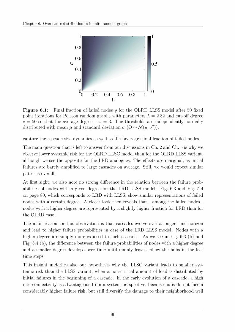
Chapter 6. Overload redistribution in infinite random graphs
µ
σ
0 0.2 0.4 0.6 0.8 10
0.2
0.4
0.6
0.8
1
0
0.5
1
Figure 6.1: Final fraction of failed nodes % for the OLRD LLSS model after 50 fixedpoint iterations for Poisson random graphs with parameters λ = 2.82 and cut-off degreec = 50 so that the average degree is z = 3. The thresholds are independently normallydistributed with mean µ and standard deviation σ (Θ ∼ N (µ, σ2)).
capture the cascade size dynamics as well as the (average) final fraction of failed nodes.
The main question that is left to answer from our discussions in Ch. 2 and Ch. 5 is why we
observe lower systemic risk for the OLRD LLSC model than for the OLRD LLSS variant,
although we see the opposite for the LRD analogues. The effects are marginal, as initial
failures are barely amplified to large cascades on average. Still, we would expect similar
patterns overall.
At first sight, we also note no strong difference in the relation between the failure prob-
abilities of nodes with a given degree for the LRD LLSS model. Fig. 6.3 and Fig. 5.4
on page 80, which corresponds to LRD with LLSS, show similar representations of failed
nodes with a certain degree. A closer look then reveals that - among the failed nodes -
nodes with a higher degree are represented by a slightly higher fraction for LRD than for
the OLRD case.
The main reason for this observation is that cascades evolve over a longer time horizon
and lead to higher failure probabilities in case of the LRD LLSS model. Nodes with a
higher degree are simply more exposed to such cascades. As we see in Fig. 6.3 (b) and
Fig. 5.4 (b), the difference between the failure probabilities of nodes with a higher degree
and a smaller degree develops over time until mainly leaves follow the hubs in the last
time steps.
This insight underlies also our hypothesis why the LLSC variant leads to smaller sys-
temic risk than the LLSS variant, when a non-critical amount of load is distributed by
initial failures in the beginning of a cascade. In the early evolution of a cascade, a high
interconnectivity is advantageous from a system perspective, because hubs do not face a
considerably higher failure risk, but still diversify the damage to their neighborhood well
90
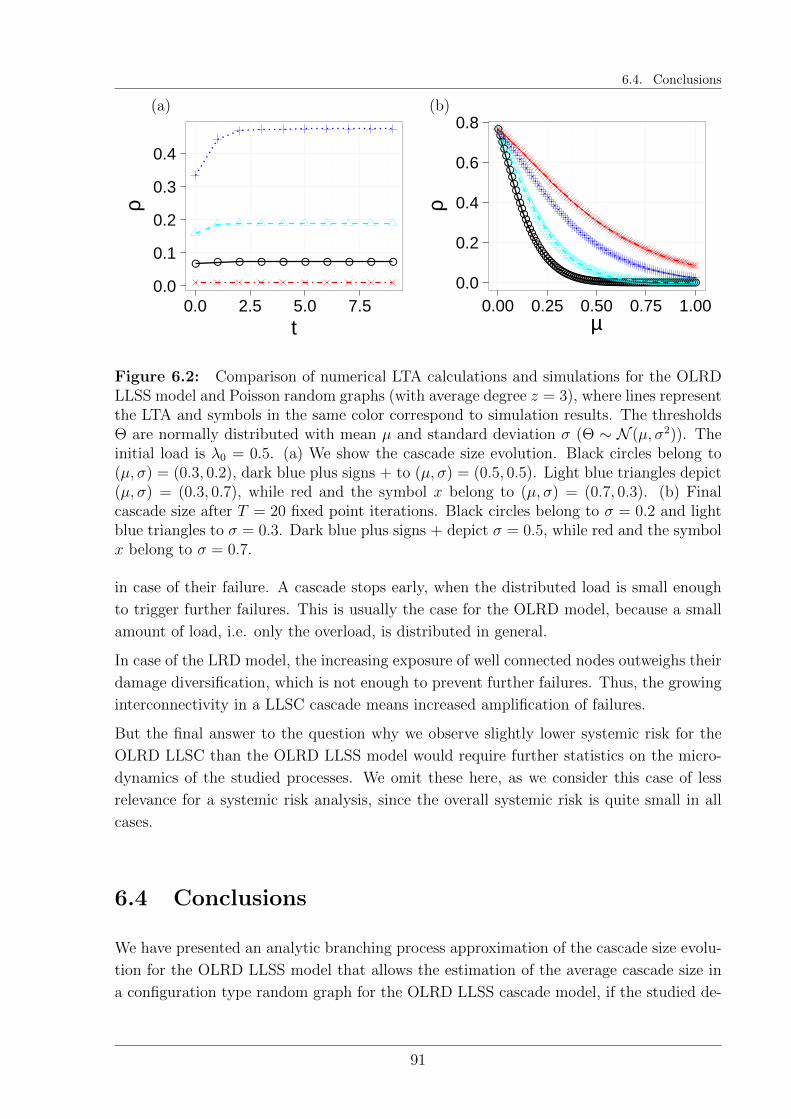
6.4. Conclusions
0.0
0.1
0.2
0.3
0.4
0.0 2.5 5.0 7.5t
ρ0.0
0.2
0.4
0.6
0.8
0.00 0.25 0.50 0.75 1.00µ
ρ
(a) (b)
Figure 6.2: Comparison of numerical LTA calculations and simulations for the OLRDLLSS model and Poisson random graphs (with average degree z = 3), where lines representthe LTA and symbols in the same color correspond to simulation results. The thresholdsΘ are normally distributed with mean µ and standard deviation σ (Θ ∼ N (µ, σ2)). Theinitial load is λ0 = 0.5. (a) We show the cascade size evolution. Black circles belong to(µ, σ) = (0.3, 0.2), dark blue plus signs + to (µ, σ) = (0.5, 0.5). Light blue triangles depict(µ, σ) = (0.3, 0.7), while red and the symbol x belong to (µ, σ) = (0.7, 0.3). (b) Finalcascade size after T = 20 fixed point iterations. Black circles belong to σ = 0.2 and lightblue triangles to σ = 0.3. Dark blue plus signs + depict σ = 0.5, while red and the symbolx belong to σ = 0.7.
in case of their failure. A cascade stops early, when the distributed load is small enough
to trigger further failures. This is usually the case for the OLRD model, because a small
amount of load, i.e. only the overload, is distributed in general.
In case of the LRD model, the increasing exposure of well connected nodes outweighs their
damage diversification, which is not enough to prevent further failures. Thus, the growing
interconnectivity in a LLSC cascade means increased amplification of failures.
But the final answer to the question why we observe slightly lower systemic risk for the
OLRD LLSC than the OLRD LLSS model would require further statistics on the micro-
dynamics of the studied processes. We omit these here, as we consider this case of less
relevance for a systemic risk analysis, since the overall systemic risk is quite small in all
cases.
6.4 Conclusions
We have presented an analytic branching process approximation of the cascade size evolu-
tion for the OLRD LLSS model that allows the estimation of the average cascade size in
a configuration type random graph for the OLRD LLSS cascade model, if the studied de-
91

Chapter 6. Overload redistribution in infinite random graphs
0.00
0.05
0.10
0.15
0.20
0.25
1 2 3 4 5 6 7 8 9 10 11 12k
P(
s=1;
k )
timet0t1t2t3t4t5t6t7t8funct
0.00
0.25
0.50
0.75
1.00
1 2 3 4 5 6 7 8 9 10 11 12k
P(
s=1
| k )
timet0t1t2t3t4t5t6t7t8funct
(a) (b)
Figure 6.3: Time evolution of failures for Poisson random graphs (with average degreez = 3) obtained by an LTA for the OLRD LLSS model. The thresholds are independentlynormally distributed with mean µ = 0.3 and standard deviation σ = 0.7. The colorindicates the time of failure of the respective fraction of failed nodes. (a) Probability thata node has degree k and is failed at the time indicated by the color. (b) Probability thata node with degree k fails at the time indicated by the color.
gree distribution has a finite second moment. This approach can be generalized to capture
also models of OLRD type where the load is not equally distributed among the functional
network neighbors, but instead in heterogeneous proportions.
Furthermore, we have discussed in more depth an explanation for the observation that the
OLRD LLSC model leads to lower systemic risk than the OLRD LLSS model, although
the opposite holds for their LRD counterparts. For the studied threshold distributions
and parameters, the OLRD model leads usually to small amounts of load distributions in
the first steps of a cascade. A stronger damage diversification of these small amounts, as
in case of the LLSC model, can then prevent further failures and stop a cascade process
early on. In the LRD LLSC model, the increased exposure of well connected nodes to
neighboring failures outweighs the damage diversification effect in case of their failure,
because the distributed load is still enough to trigger additional failures. Interestingly, the
trade-off between increased damage diversification and increased exposure to failures by
hubs is especially relevant in the early stages of a cascade.
92
“Everything should be made as simple as possible, but not simpler.”
Albert Einstein
Part II
Extensions and limitations of
modeling assumptions
93


Introduction
Introduction
In Part II, we study extensions of the cascade models in the framework of Part I. For
simplicity, we often focus on the simplest case, the CL ED model. Still, our derivations
can be transferred to the other model classes as well.
We are mainly interested in the question how robust are results are in general with respect
to changes in our modeling assumptions. We challenge this way our previous findings and
test, whether more knowledge is required about systems to make reasonable estimations
of inherent systemic risk.
We face the problem that the models under investigation are highly-nonlinear, discontin-
uous and show critical or chaotic behavior. This means, we cannot argue in a fashion that
we study a particular effect, e.g., the diversification behavior of nodes with a given degree
distribution and add model complexity, for instance we consider furthermore degree-degree
correlations, a second network layer, or systemic feedback. And then, the difference be-
tween the new results and old results without the model extension can simply be attributed
to the new effect. Instead, the results for both effects, the old and new, do not simply add
up to a new observation as for linear models. The effects interfere, amplify or dampen
each other.
Because of this, we study next three aspects that we find critical in our previous investi-
gations.
First, we ask for the consequences of simplifying network structures. As we have mentioned
in Ch. 2, a network is a model for interaction or dependency patterns between similar
components in a system. Usually, these interactions do not follow the exact same rules.
Because of this, we study in Ch. 7, what happens if we introduce a second network layer
and another type of link. This introduces a feedback mechanism between the two network
layers.
In Ch. 8, we further ask for the consequences if a similar feedback does not result from a
different network layer. Instead, the thresholds of nodes are coupled to the macro state of
the system, thus respond to global information on the cascade size evolution. This could
be also interpreted as global load distribution that shows similarities with LRD models
on fully connected networks. Thus, we investigate the variability of our cascade model
95

Chapter 6. Introduction
classes.
Ch. 9 we devote to the weakest point of our branching process approximation, which
assumes infinitely large networks. These serve as estimate of the average cascade size. But
we show by several examples that a focus on infinite networks crucially underestimates
the variability of cascade outcomes in finite systems. The size of a system clearly needs
to be considered in the design or control of its interdependencies.
96
Chapter 7
Systemic risk in multiplex networks
with asymmetric coupling and
threshold feedback
Summary
We study cascades on a two-layer multiplex network, with asymmetric feedbackthat depends on the coupling strength between the layers. In this extension,we focus on the Constant Load Exposure Diversification model on each layer.Based on an analytical branching process approximation, we calculate the sys-temic risk measured by the final fraction of failed nodes on a reference layer.The results are compared with the case of a single layer network that is anaggregated representation of the two layers. We find that systemic risk in thetwo-layer network is smaller than in the aggregated one only if the couplingstrength between the two layers is small. Above a critical coupling strength,systemic risk is increased because of the mutual amplification of cascades inthe two layers. We even observe sharp phase transitions in the cascade sizethat are less pronounced on the aggregated layer. Our insights relate to a sce-nario where firms decide whether they want to split their business into a lessrisky core business and a more risky subsidiary business. In most cases, thismay lead to a drastic increase of systemic risk, which is underestimated in anaggregated approach.
Based on R. Burkholz, M. V. Leduc, A. Garas, and F. Schweitzer, “Systemic risk in multiplex net-works with asymmetric coupling and threshold feedback”. Physica D : 323-324, 64 - 72. RB contributedto the design of the research questions. RB derived the analytic formulas, implemented parts of the fixedpoint iterations, contributed to the interpretation of the results and the writing.
97
Chapter 7. Systemic risk in multiplex networks with asymmetric coupling and threshold feedback
7.1 Introduction
In Part I of this thesis, we have considered simplifying dependency structures that were
solely defined by the degree distribution of a network. Also the type of dependency has
been the same. Here, we get an impression how limiting this assumption can be by intro-
ducing a second network layer and interactions between those layers for one of the models
that we have introduced, the Constant Load Exposure Diversification model. Although we
follow a generic modeling approach, we motivate our model choice by firms with core and
subsidiary businesses each represented in one of the two layers. Although this application
is rather academic considering our simplifying network and process assumptions, it identi-
fies a possible application area where we would expect similar effects as we can observe in
our model. Moreover, our multiplex approach underlines that a systemic risk analysis can
be substantially misleading, if the nature of different network layers is neglected (Burkholz
et al., 2016b).
In many situations, cascading failures can be influenced by the combination of different
types of interactions between the individual components of the system. For instance, this
is the case in interbank systems, where banks are exposed to each other via different types
of financial obligations (loans, derivative contracts, etc.) (e.g. Ref. (Arinaminpathy et al.,
2012) and (Montagna and Kok, 2013)). The bankruptcy of a bank can thus cascade to
other banks in non-standard ways. Another example are firms diversifying their activities
across different business units, each of which is exposed to cascade risk in its own field of
activity.
An important question we wish to investigate in this chapter is how diversification across
different types of interactions can affect the risk of cascading failures. For that purpose,
we study the case of a firm that diversifies its activities across a core-business unit and a
subsidiary-business unit. Each business unit is exposed to other firms’ business units in
the same sector of business activity (either core or subsidiary). This means that a business
unit can fail (i.e. go bankrupt) as a result of a cascade of failures (i.e. bankruptcies) in
the same sector of business activity.
The question of the structuring of a firm into sub-units has been studied from a different
angle in the financial economics literature (e.g. (Lewellen, 1971) and (Maksimovic and
Phillips, 2002)) and often focuses on the efficiency of the allocation of its resources across
different industries. Another question that has received some attention is that of whether
a firm can diversify the risk of its income streams by operating in different business areas.
For example, Levy and Sarnat (1970), Smith and Schreiner (1969) and Amihud and Lev
(1981) studied how conglomerates can diversify the risk associated with their revenue
streams from the perspective of portfolio theory.
Here, we use a complex networks approach and we view the system of firm activities as an
98
7.2. Model
interconnected multi-layered network (see (D’Agostino and Scala, 2014; Gao et al., 2012;
Garas, 2015; Kivela et al., 2014)). The distinct layers of this network contain individual
networks defined by a particular type of interaction according to a given business activity,
while the inter-connections between layers allow for cross-layer interactions. In this setting
we develop a model where failures (i.e. bankruptcies) on two different network layers
affect firms asymmetrically: The first layer represents exposures between the firms in the
core business while the second layer represents exposures between firms in the subsidiary
business. Failure (i.e. bankruptcy) of a firm’s core business unit implies failure of its
subsidiary business unit, whereas failure of a firm’s subsidiary business unit only causes
a shock to the firm’s resistance threshold in its core business unit (see Fig. 7.1 for an
illustration). We find that when the coupling strength from the core to the subsidiary
layer is varied only slightly, there is a sharp transition between a safe regime, where
there is no cascade of failures, and a catastrophic regime, where there is a full cascade
of failures. Moreover, when comparing the two-layer network to the single-layer network
formed by aggregating the two layers, we find that cascades can be larger on the two-layer
network than on the aggregated one. On the other hand, by varying the strength of the
feedback between the two layers, we identify the existence of a regime where the two-layer
network is safer than the aggregated one and another regime where the reverse holds. This
points to the critical importance of the coupling of the layers when structuring a firm into
different business units. Also, dealing with aggregated network data that ignores the fine
structure of the coupling between different layers can lead to significant underestimation
or overestimation of cascade risk.
This Chapter is structured as follows. In Sec. 7.2, we describe the two-layer cascade
model. In Sec. 7.3, we derive a branching process approximation as an approximation for
large networks and use it to analyze the aforementioned phenomena. These phenomena
are presented in Sec. 7.4 where we compare our analytical results with simulations and
analyze further the observed phase transitions. In Sec. 7.5, we conclude and interpret the
consequences of our theoretical investigations for the application to networks of firms that
might decide about merging their core and their subsidiary business.
7.2 Model
We first consider a finite model with N firms. Each firm can be represented by a node
i present on each of two different layers: layer 0 (the core-business layer) and layer 1
(the subsidiary-business layer). Each layer l ∈ 0, 1 has a topology represented by an
adjacency matrix Gl. On each layer l, node i can be in one of two states sil ∈ 0, 1, healthy
(sil = 0) or failed (sil = 1). si0 = 1 represents the bankruptcy of firm i’s core-business unit,
whereas si1 = 1 represents the bankruptcy of its subsidiary-business unit. This state is
determined by two other variables as in the previous chapters: a node’s fragility or loss on
99
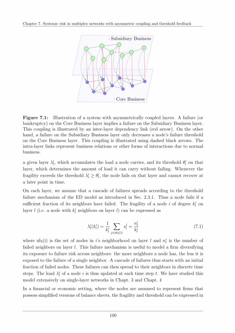
Chapter 7. Systemic risk in multiplex networks with asymmetric coupling and threshold feedback
Core Business
Subsidiary Business
Figure 7.1: Illustration of a system with asymmetrically coupled layers. A failure (orbankruptcy) on the Core Business layer implies a failure on the Subsidiary Business layer.This coupling is illustrated by an inter-layer dependency link (red arrow). On the otherhand, a failure on the Subsidiary Business layer only decreases a node’s failure thresholdon the Core Business layer. This coupling is illustrated using dashed black arrows. Theintra-layer links represent business relations or other forms of interactions due to normalbusiness.
a given layer λil, which accumulates the load a node carries, and its threshold θil on that
layer, which determines the amount of load it can carry without failing. Whenever the
fragility exceeds the threshold λil ≥ θil , the node fails on that layer and cannot recover at
a later point in time.
On each layer, we assume that a cascade of failures spreads according to the threshold
failure mechanism of the ED model as introduced in Sec. 2.3.1. Thus a node fails if a
sufficient fraction of its neighbors have failed. The fragility of a node i of degree kil on
layer l (i.e. a node with kil neighbors on layer l) can be expressed as
λil(kil) =
1
kil
∑j∈nbl(i)
sjl =nilkil
(7.1)
where nbl(i) is the set of nodes in i’s neighborhood on layer l and nil is the number of
failed neighbors on layer l. This failure mechanism is useful to model a firm diversifying
its exposure to failure risk across neighbors: the more neighbors a node has, the less it is
exposed to the failure of a single neighbor. A cascade of failures thus starts with an initial
fraction of failed nodes. These failures can then spread to their neighbors in discrete time
steps. The load λil of a node i is thus updated at each time step t. We have studied this
model extensively on single-layer networks in Chapt. 3 and Chapt. 4
In a financial or economic setting, where the nodes are assumed to represent firms that
possess simplified versions of balance sheets, the fragility and threshold can be expressed in
100
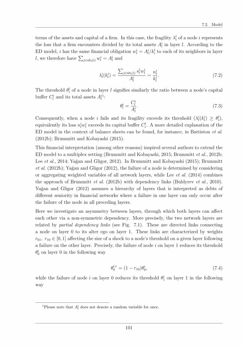
7.2. Model
terms of the assets and capital of a firm. In this case, the fragility λli of a node i represents
the loss that a firm encounters divided by its total assets Ail in layer l. According to the
ED model, i has the same financial obligation wil = Ail/kli to each of its neighbors in layer
l, we therefore have∑
j∈nbl(i)wil = Ail and
λil(kil) =
∑j∈nbl(i)
sjlwil
Ail=nilkil. (7.2)
The threshold θli of a node in layer l signifies similarly the ratio between a node’s capital
buffer Cil and its total assets Ail
1:
θil =Cil
Ail. (7.3)
Consequently, when a node i fails and its fragility exceeds its threshold (λil(kil) ≥ θli),
equivalently its loss nilwil exceeds its capital buffer C l
i . A more detailed explanation of the
ED model in the context of balance sheets can be found, for instance, in Battiston et al.
(2012b); Brummitt and Kobayashi (2015).
This financial interpretation (among other reasons) inspired several authors to extend the
ED model to a multiplex setting (Brummitt and Kobayashi, 2015; Brummitt et al., 2012b;
Lee et al., 2014; Yagan and Gligor, 2012). In Brummitt and Kobayashi (2015); Brummitt
et al. (2012b); Yagan and Gligor (2012), the failure of a node is determined by considering
or aggregating weighted variables of all network layers, while Lee et al. (2014) combines
the approach of Brummitt et al. (2012b) with dependency links (Buldyrev et al., 2010).
Yagan and Gligor (2012) assumes a hierarchy of layers that is interpreted as debts of
different seniority in financial networks where a failure in one layer can only occur after
the failure of the node in all preceding layers.
Here we investigate an asymmetry between layers, through which both layers can affect
each other via a non-symmetric dependency. More precisely, the two network layers are
related by partial dependency links (see Fig. 7.1). These are directed links connecting
a node on layer 0 to its alter ego on layer 1. These links are characterized by weights
r01, r10 ∈ [0, 1] affecting the size of a shock to a node’s threshold on a given layer following
a failure on the other layer. Precisely, the failure of node i on layer 1 reduces its threshold
θi0 on layer 0 in the following way
θi,r0 = (1− r10)θi0, (7.4)
while the failure of node i on layer 0 reduces its threshold θi1 on layer 1 in the following
way
1Please note that Ail does not denote a random variable for once.
101
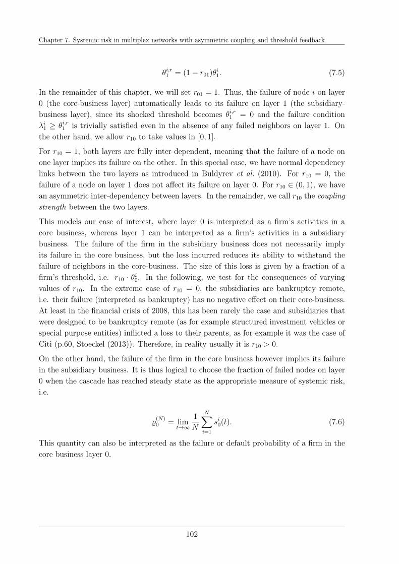
Chapter 7. Systemic risk in multiplex networks with asymmetric coupling and threshold feedback
θi,r1 = (1− r01)θi1. (7.5)
In the remainder of this chapter, we will set r01 = 1. Thus, the failure of node i on layer
0 (the core-business layer) automatically leads to its failure on layer 1 (the subsidiary-
business layer), since its shocked threshold becomes θi,r1 = 0 and the failure condition
λi1 ≥ θi,r1 is trivially satisfied even in the absence of any failed neighbors on layer 1. On
the other hand, we allow r10 to take values in [0, 1].
For r10 = 1, both layers are fully inter-dependent, meaning that the failure of a node on
one layer implies its failure on the other. In this special case, we have normal dependency
links between the two layers as introduced in Buldyrev et al. (2010). For r10 = 0, the
failure of a node on layer 1 does not affect its failure on layer 0. For r10 ∈ (0, 1), we have
an asymmetric inter-dependency between layers. In the remainder, we call r10 the coupling
strength between the two layers.
This models our case of interest, where layer 0 is interpreted as a firm’s activities in a
core business, whereas layer 1 can be interpreted as a firm’s activities in a subsidiary
business. The failure of the firm in the subsidiary business does not necessarily imply
its failure in the core business, but the loss incurred reduces its ability to withstand the
failure of neighbors in the core-business. The size of this loss is given by a fraction of a
firm’s threshold, i.e. r10 · θi0. In the following, we test for the consequences of varying
values of r10. In the extreme case of r10 = 0, the subsidiaries are bankruptcy remote,
i.e. their failure (interpreted as bankruptcy) has no negative effect on their core-business.
At least in the financial crisis of 2008, this has been rarely the case and subsidiaries that
were designed to be bankruptcy remote (as for example structured investment vehicles or
special purpose entities) inflicted a loss to their parents, as for example it was the case of
Citi (p.60, Stoeckel (2013)). Therefore, in reality usually it is r10 > 0.
On the other hand, the failure of the firm in the core business however implies its failure
in the subsidiary business. It is thus logical to choose the fraction of failed nodes on layer
0 when the cascade has reached steady state as the appropriate measure of systemic risk,
i.e.
%(N)0 = lim
t→∞
1
N
N∑i=1
si0(t). (7.6)
This quantity can also be interpreted as the failure or default probability of a firm in the
core business layer 0.
102
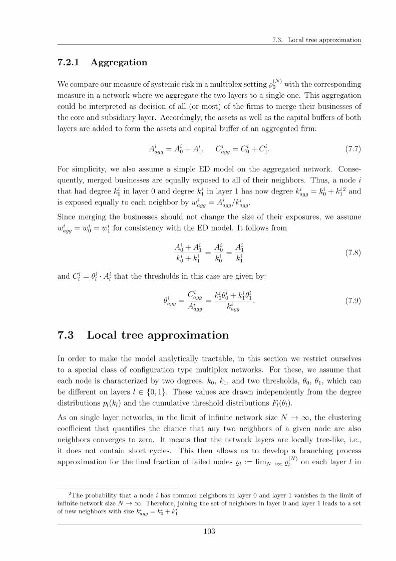
7.3. Local tree approximation
7.2.1 Aggregation
We compare our measure of systemic risk in a multiplex setting %(N)0 with the corresponding
measure in a network where we aggregate the two layers to a single one. This aggregation
could be interpreted as decision of all (or most) of the firms to merge their businesses of
the core and subsidiary layer. Accordingly, the assets as well as the capital buffers of both
layers are added to form the assets and capital buffer of an aggregated firm:
Aiagg = Ai0 + Ai1, Ciagg = Ci
0 + Ci1. (7.7)
For simplicity, we also assume a simple ED model on the aggregated network. Conse-
quently, merged businesses are equally exposed to all of their neighbors. Thus, a node i
that had degree ki0 in layer 0 and degree ki1 in layer 1 has now degree kiagg = ki0 + ki12 and
is exposed equally to each neighbor by wiagg = Aiagg/kiagg.
Since merging the businesses should not change the size of their exposures, we assume
wiagg = wi0 = wi1 for consistency with the ED model. It follows from
Ai0 + Ai1ki0 + ki1
=Ai0ki0
=Ai1ki1
(7.8)
and Cil = θil · Ail that the thresholds in this case are given by:
θiagg =Ciagg
Aiagg=ki0θ
i0 + ki1θ
i1
kiagg. (7.9)
7.3 Local tree approximation
In order to make the model analytically tractable, in this section we restrict ourselves
to a special class of configuration type multiplex networks. For these, we assume that
each node is characterized by two degrees, k0, k1, and two thresholds, θ0, θ1, which can
be different on layers l ∈ 0, 1. These values are drawn independently from the degree
distributions pl(kl) and the cumulative threshold distributions Fl(θl).
As on single layer networks, in the limit of infinite network size N → ∞, the clustering
coefficient that quantifies the chance that any two neighbors of a given node are also
neighbors converges to zero. It means that the network layers are locally tree-like, i.e.,
it does not contain short cycles. This then allows us to develop a branching process
approximation for the final fraction of failed nodes %l := limN→∞ %(N)l on each layer l in
2The probability that a node i has common neighbors in layer 0 and layer 1 vanishes in the limit ofinfinite network size N →∞. Therefore, joining the set of neighbors in layer 0 and layer 1 leads to a setof new neighbors with size kiagg = ki0 + ki1.
103
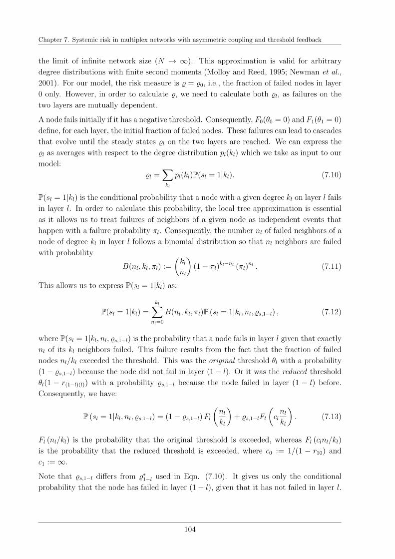
Chapter 7. Systemic risk in multiplex networks with asymmetric coupling and threshold feedback
the limit of infinite network size (N → ∞). This approximation is valid for arbitrary
degree distributions with finite second moments (Molloy and Reed, 1995; Newman et al.,
2001). For our model, the risk measure is % = %0, i.e., the fraction of failed nodes in layer
0 only. However, in order to calculate %, we need to calculate both %l, as failures on the
two layers are mutually dependent.
A node fails initially if it has a negative threshold. Consequently, F0(θ0 = 0) and F1(θ1 = 0)
define, for each layer, the initial fraction of failed nodes. These failures can lead to cascades
that evolve until the steady states %l on the two layers are reached. We can express the
%l as averages with respect to the degree distribution pl(kl) which we take as input to our
model:
%l =∑kl
pl(kl)P(sl = 1|kl). (7.10)
P(sl = 1|kl) is the conditional probability that a node with a given degree kl on layer l fails
in layer l. In order to calculate this probability, the local tree approximation is essential
as it allows us to treat failures of neighbors of a given node as independent events that
happen with a failure probability πl. Consequently, the number nl of failed neighbors of a
node of degree kl in layer l follows a binomial distribution so that nl neighbors are failed
with probability
B(nl, kl, πl) :=
(klnl
)(1− πl)kl−nl (πl)
nl . (7.11)
This allows us to express P(sl = 1|kl) as:
P(sl = 1|kl) =
kl∑nl=0
B(nl, kl, πl)P (sl = 1|kl, nl, %s,1−l) , (7.12)
where P(sl = 1|kl, nl, %s,1−l) is the probability that a node fails in layer l given that exactly
nl of its kl neighbors failed. This failure results from the fact that the fraction of failed
nodes nl/kl exceeded the threshold. This was the original threshold θl with a probability
(1− %s,1−l) because the node did not fail in layer (1− l). Or it was the reduced threshold
θl(1 − r(1−l)(l)) with a probability %s,1−l because the node failed in layer (1 − l) before.
Consequently, we have:
P (sl = 1|kl, nl, %s,1−l) = (1− %s,1−l)Fl(nlkl
)+ %s,1−lFl
(clnlkl
). (7.13)
Fl (nl/kl) is the probability that the original threshold is exceeded, whereas Fl (clnl/kl)
is the probability that the reduced threshold is exceeded, where c0 := 1/(1 − r10) and
c1 :=∞.
Note that %s,1−l differs from %∗1−l used in Eqn. (7.10). It gives us only the conditional
probability that the node has failed in layer (1− l), given that it has not failed in layer l.
104
7.3. Local tree approximation
It depends on a neighbor’s failure probability on the other layer, π∗1−l, via
%s,1−l =∑k1−l
p1−l(k1−l)
k1−l∑nl=0
B(nl, k1−l, π∗1−l) F1−l
(n1−l
k1−l
). (7.14)
Eqn. (7.14) has the same structure as the branching process approximation for the fraction
of failed nodes on single layers (Gleeson and Cahalane, 2007). It also has a structure
similar to Eqs. (7.10)-(7.12), with the only difference of a simpler response function, i.e.,
P(sl = 1|kl, nl, %s,1−l) = F1−l(n1−l/k1−l), which is the probability that the fraction of failed
neighbors exceeds the original threshold in layer (1− l).
In order to compute Eqn. (7.12), we need to know the failure probability πl of a neighbor
in layer l. To achieve this, we iteratively solve a system of coupled fixed-point equations
for the probabilities πl, defined as
πl = Ll (πl) :=1
zl
∑kl
pl(kl)kl
kl−1∑nl=0
B(nl, kl − 1, πl)P (sl = 1|kl, nl, %s,1−l) (7.15)
where zl =∑
klpl(kl)kl and P(sl = 1|kl, nl, %s,1−l) is defined by Eqn. (7.13)
We note again similarities between Eqn. (7.15) that describes the failure probability of a
neighbor and Eqs. (7.10), (7.13) that describe the failure probability of a node, but also
two main differences:
The first difference is that in Eqn. (7.15) the degree distribution of a neighbor follows
pl(kl)kl/zl instead of pl(kl) for a node (Newman, 2010), analogously to single network
layers. It is proportional to the degree kl, since every link of a neighbor increases the
probability of the neighbor to be connected to the node under consideration, i.e. a ran-
domly selected node that fails with probability %l in layer l.
The second difference is that the binomial distribution in Eqn. (7.15) depends on kl − 1
instead of kl because we have to take into account the neighbors of the neighbors of the
node under consideration in order to determine the failure probability of the node’s direct
neighbors. The set of all neighbors of a node is also called its first order neighborhood,
while the set of neighbors of the neighbors the node’s second order neighborhood. We take
the failure probability of a neighbor as input to calculate the failure probability of the
node under consideration as in Eqs. (7.10), (7.13). Therefore, πl is conditioned on the
event that the node under consideration has not failed before the neighbor. Only kl − 1
neighbors of the neighbor with degree kl can have possibly failed before, because the node
under consideration is a neighbor of this neighbor.
105
Chapter 7. Systemic risk in multiplex networks with asymmetric coupling and threshold feedback
7.3.1 Aggregation
The fraction of failed nodes on a single aggregated layer %agg can be computed with less
effort and with a similar approach as in Gleeson and Cahalane (2007), although the thresh-
olds depend on the nodes’ degrees as in Burkholz et al. (2016a).
For given degrees k0 in layer 0 and k1 in layer 1 we denote the cumulative distribution
function of θagg by F(k0,k1)agg to signify its degree dependence. Then we iteratively solve the
scalar fixed point equation
πagg =∑k0,k1
p0(k0)p1(k1) (k0 + k1)
z0 + z1
×
×k0+k1−1∑nagg=0
B(nagg, k0 + k1 − 1, πagg)F(k0,k1)agg
(nagg
k0 + k1
) (7.16)
for the failure probability of a node’s neighbor πagg. Then, its solution π∗agg serves as input
for the calculation of the average fraction of failed nodes on the aggregated network using:
%agg =∑k0,k1
p0(k0)p1(k1)
k0+k1−1∑nagg=0
B(nagg, k0 + k1 − 1, π∗agg)F(k0,k1)agg
(nagg
k0 + k1
). (7.17)
7.4 Results
7.4.1 Comparison with computer simulations
We now compare our numerical solution of the fixed point equations (7.15) for the mul-
tiplex model with computer simulations, using the illustrative case of an uncorrelated,
two-layer Erdos-Renyi network (Erdos and Renyi, 1959). For the computer simulations,
we implement the time-dependent model as described in Sec. 7.2, i.e. we simulate the
evolution of cascades until they reach the steady state. The network size is N = 10, 000
for each layer. Further, we sample over 100 network realizations for every initial condition.
The degree distributions pl(kl) on each layer are approximately Poisson distributions
pl(kl) =zkllkl!
e−zl (7.18)
with identical mean degrees z0 = z1. The thresholds are normally distributed, i.e. θ0 ∼N (µ0, σ
20) and θ1 ∼ N (µ1, σ
21) with different parameters µl, σl. In our case, we fix the
threshold distribution on layer 0 to parameters µ0 = 0.3 and σ0 = 0.1, which ensures that
the failure probability for the nodes in an uncoupled network would be very small, to be
106
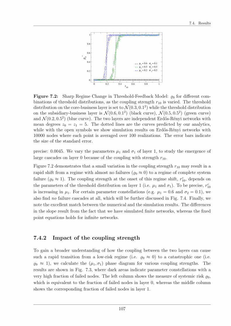
7.4. Results
0 0.2 0.4 0.6 0.8 1r10
0
0.2
0.4
0.6
0.8
1
ρ0
*
µ1 = 0.6 σ
1 = 0.1
µ1 = 0.5 σ
1 = 0.5
µ1 = 0.2 σ
1= 0.5
Figure 7.2: Sharp Regime Change in Threshold-Feedback Model: %0 for different com-binations of threshold distributions, as the coupling strength r10 is varied. The thresholddistribution on the core-business layer is set toN (0.3, 0.12) while the threshold distributionon the subsidiary-business layer is N (0.6, 0.12) (black curve), N (0.5, 0.52) (green curve)and N (0.2, 0.52) (blue curve). The two layers are independent Erdos-Renyi networks withmean degrees z0 = z1 = 5. The dotted lines are the curves predicted by our analytics,while with the open symbols we show simulation results on Erdos-Renyi networks with10000 nodes where each point is averaged over 100 realizations. The error bars indicatethe size of the standard error.
precise: 0.0045. We vary the parameters µ1 and σ1 of layer 1, to study the emergence of
large cascades on layer 0 because of the coupling with strength r10.
Figure 7.2 demonstrates that a small variation in the coupling strength r10 may result in a
rapid shift from a regime with almost no failures (%0 ≈ 0) to a regime of complete system
failure (%0 ≈ 1). The coupling strength at the onset of this regime shift, rc10, depends on
the parameters of the threshold distribution on layer 1 (i.e. µ1 and σ1). To be precise, rc10
is increasing in µ1. For certain parameter constellations (e.g. µ1 = 0.6 and σ2 = 0.1), we
also find no failure cascades at all, which will be further discussed in Fig. 7.4. Finally, we
note the excellent match between the numerical and the simulation results. The differences
in the slope result from the fact that we have simulated finite networks, whereas the fixed
point equations holds for infinite networks.
7.4.2 Impact of the coupling strength
To gain a broader understanding of how the coupling between the two layers can cause
such a rapid transition from a low-risk regime (i.e. %0 ≈ 0) to a catastrophic one (i.e.
%0 ≈ 1), we calculate the (µ1, σ1) phase diagram for various coupling strengths. The
results are shown in Fig. 7.3, where dark areas indicate parameter constellations with a
very high fraction of failed nodes. The left column shows the measure of systemic risk %0,
which is equivalent to the fraction of failed nodes in layer 0, whereas the middle column
shows the corresponding fraction of failed nodes in layer 1.
107
Chapter 7. Systemic risk in multiplex networks with asymmetric coupling and threshold feedback
As a reference case, the right column shows a single-layer network, which we constructed in
order to put the results for the two-layer network into perspective. Nodes in this combined
single-layer network have a degree kagg = k0 +k1 and a threshold θagg = (k0θ0 +k1θ1)/(k0 +
k1), as we discussed already in Sec. 7.2.1, by deriving a node’s new balance sheet that
results from merging the core business and the subsidiary.
In Sec. 7.3.1 we have explained how to compute our systemic risk measure from the given
degree distributions. Since in our example the thresholds θ0 and θ1 follow independent
normal distributions, the aggregated thresholds are normally distributed as well for given
degrees k0 and k1. Their distribution can be found by taking the convolution of the
probability density functions of θ0k0/(k0 + k1) and θ1k1/(k0 + k1). This yields θagg ∼N (µagg, σ
2agg), where µagg = (µ0k0 + µ1k1)/(k0 + k1) and σagg =
√(σ0k0)2 + (σ1k1)2/(k0 +
k1).
Our reference case is motivated by two considerations: (a) We want to estimate the error
made if a multiplex network is approximated by a single layer network, i.e. the properties
of the different layers are simply aggregated in one layer. (b) For the application scenario at
hand, namely the management decision of firms to merge their core and subsidiary business
units into one business, we want to understand the impact on the resulting risk exposure.
To calculate the phase diagram, we assume that all firms make the same decision, which
for example could be motivated by herding behavior.
Since we vary only (µ1, σ1), we plot all phase diagrams with respect to these two param-
eters. Because the combined layer network no longer contains the coupling strength r10,
the respective phase plots do not change by varying r10. They are merely repeated for the
purpose of comparison with the other columns. We hypothesize that nodes in the com-
bined layer network have a smaller failure probability compared to the two-layer network
because they share their capital buffers. Their degree is also larger, which additionally
implies that the risk is better diversified among the neighbors. On the other hand, be-
cause of the larger degrees, there is a higher connectivity in the combined layer network.
This has the potential to amplify small cascades more than in the less connected separate
layers. We will investigate, by means of numerical solutions of the fixed point equations,
which of these antagonistic effects may dominate in a given parameter region.
By comparing the first and third columns in Fig. 7.3, we can identify a different risk
profile for small and for large coupling strengths. For small values of r10 the cascades on
layer 1 cannot propagate to layer 0, therefore we do not observe any systemic risk. This is
different for the combined layer network, where large cascades can occur for a small range
of parameters.
The picture is inverted for larger values of r10. Here we find, by increasing r10, an increasing
region of high systemic risk that is driven by the mutual amplification of cascades between
the two layers. This leads to a very sharp phase transition, i.e. a clear separation of regions
108

7.4. Results
%0 %1 %∗agg
r10 = 0
µ1
0 0.2 0.4 0.6 0.8 1
σ1
0
0.2
0.4
0.6
0.8
1
0
0.5
1
µ1
0 0.2 0.4 0.6 0.8 1
σ1
0
0.2
0.4
0.6
0.8
1
0
0.5
1
µ1
0 0.2 0.4 0.6 0.8 1
σ1
0
0.2
0.4
0.6
0.8
1
0
0.5
1
r10 = 0.2
µ1
0 0.2 0.4 0.6 0.8 1
σ1
0
0.2
0.4
0.6
0.8
1
0
0.5
1
µ1
0 0.2 0.4 0.6 0.8 1
σ1
0
0.2
0.4
0.6
0.8
1
0
0.5
1
µ1
0 0.2 0.4 0.6 0.8 1
σ1
0
0.2
0.4
0.6
0.8
1
0
0.5
1
r10 = 0.4
µ1
0 0.2 0.4 0.6 0.8 1
σ1
0
0.2
0.4
0.6
0.8
1
0
0.5
1
µ1
0 0.2 0.4 0.6 0.8 1
σ1
0
0.2
0.4
0.6
0.8
1
0
0.5
1
µ1
0 0.2 0.4 0.6 0.8 1
σ1
0
0.2
0.4
0.6
0.8
1
0
0.5
1
r10 = 0.8
µ1
0 0.2 0.4 0.6 0.8 1
σ1
0
0.2
0.4
0.6
0.8
1
0
0.5
1
µ1
0 0.2 0.4 0.6 0.8 1
σ1
0
0.2
0.4
0.6
0.8
1
0
0.5
1
µ1
0 0.2 0.4 0.6 0.8 1
σ1
0
0.2
0.4
0.6
0.8
1
0
0.5
1
r10 = 1.0
µ1
0 0.2 0.4 0.6 0.8 1
σ1
0
0.2
0.4
0.6
0.8
1
0
0.5
1
µ1
0 0.2 0.4 0.6 0.8 1
σ1
0
0.2
0.4
0.6
0.8
1
0
0.5
1
µ1
0 0.2 0.4 0.6 0.8 1
σ1
0
0.2
0.4
0.6
0.8
1
0
0.5
1
Figure 7.3: Sharp Regime Change in Threshold-Feedback Model: %0 and %1 for µ0 = 0.3,σ0 = 0.1 and (µ1, σ1) ∈ [0, 1]2 as r10 is varied. The two layers are independent Erdos-Renyinetworks with mean degrees z0 = z1 = 5 and thresholds on each layer are independentlydistributed, i.e. θ0 ∼ N (0.3, 0.12) and θ1 ∼ N (µ1, σ
21), where (µ1, σ1) ∈ [0, 1]2. %∗agg is the
fraction of failures on the aggregated network, i.e. a network where kagg = k0 + k1 andθagg = (k0θ0 + k1θ1)/(k0 + k1).
with complete breakdown and regions with no breakdown. We note that this differs from
the observation for the combined layer network, where the phase transition can also be
observed. However, there are extended regions where the systemic risk is at intermediate
levels, as indicated by the gray areas.
We also wish to identify how the onset of systemic risk on layer 0 depends on the coupling
109
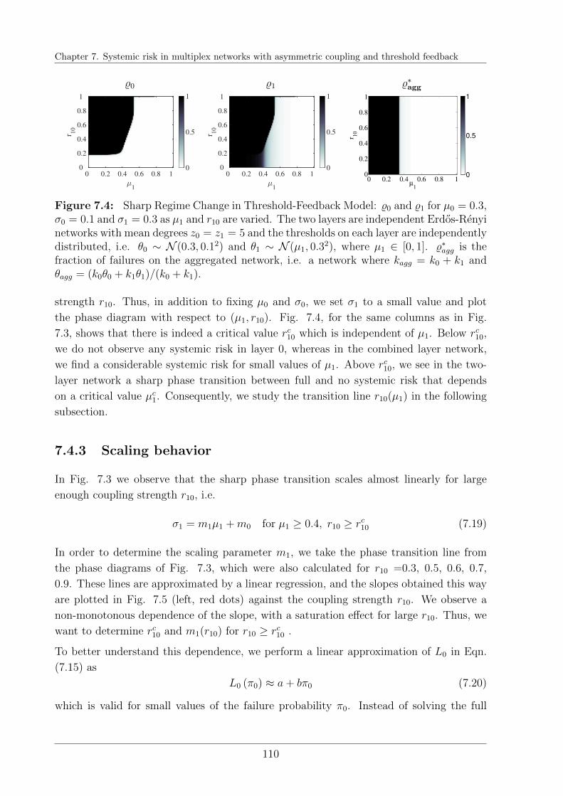
Chapter 7. Systemic risk in multiplex networks with asymmetric coupling and threshold feedback
%0 %1 %∗agg
µ1
0 0.2 0.4 0.6 0.8 1
r 10
0
0.2
0.4
0.6
0.8
1
0
0.5
1
µ1
0 0.2 0.4 0.6 0.8 1
r 10
0
0.2
0.4
0.6
0.8
1
0
0.5
1
µ1
r 10
0 0.2 0.4 0.6 0.8 10
0.2
0.4
0.6
0.8
1
0
0.5
1
Figure 7.4: Sharp Regime Change in Threshold-Feedback Model: %0 and %1 for µ0 = 0.3,σ0 = 0.1 and σ1 = 0.3 as µ1 and r10 are varied. The two layers are independent Erdos-Renyinetworks with mean degrees z0 = z1 = 5 and the thresholds on each layer are independentlydistributed, i.e. θ0 ∼ N (0.3, 0.12) and θ1 ∼ N (µ1, 0.3
2), where µ1 ∈ [0, 1]. %∗agg is thefraction of failures on the aggregated network, i.e. a network where kagg = k0 + k1 andθagg = (k0θ0 + k1θ1)/(k0 + k1).
strength r10. Thus, in addition to fixing µ0 and σ0, we set σ1 to a small value and plot
the phase diagram with respect to (µ1, r10). Fig. 7.4, for the same columns as in Fig.
7.3, shows that there is indeed a critical value rc10 which is independent of µ1. Below rc10,
we do not observe any systemic risk in layer 0, whereas in the combined layer network,
we find a considerable systemic risk for small values of µ1. Above rc10, we see in the two-
layer network a sharp phase transition between full and no systemic risk that depends
on a critical value µc1. Consequently, we study the transition line r10(µ1) in the following
subsection.
7.4.3 Scaling behavior
In Fig. 7.3 we observe that the sharp phase transition scales almost linearly for large
enough coupling strength r10, i.e.
σ1 = m1µ1 +m0 for µ1 ≥ 0.4, r10 ≥ rc10 (7.19)
In order to determine the scaling parameter m1, we take the phase transition line from
the phase diagrams of Fig. 7.3, which were also calculated for r10 =0.3, 0.5, 0.6, 0.7,
0.9. These lines are approximated by a linear regression, and the slopes obtained this way
are plotted in Fig. 7.5 (left, red dots) against the coupling strength r10. We observe a
non-monotonous dependence of the slope, with a saturation effect for large r10. Thus, we
want to determine rc10 and m1(r10) for r10 ≥ rc10 .
To better understand this dependence, we perform a linear approximation of L0 in Eqn.
(7.15) as
L0 (π0) ≈ a+ bπ0 (7.20)
which is valid for small values of the failure probability π0. Instead of solving the full
110
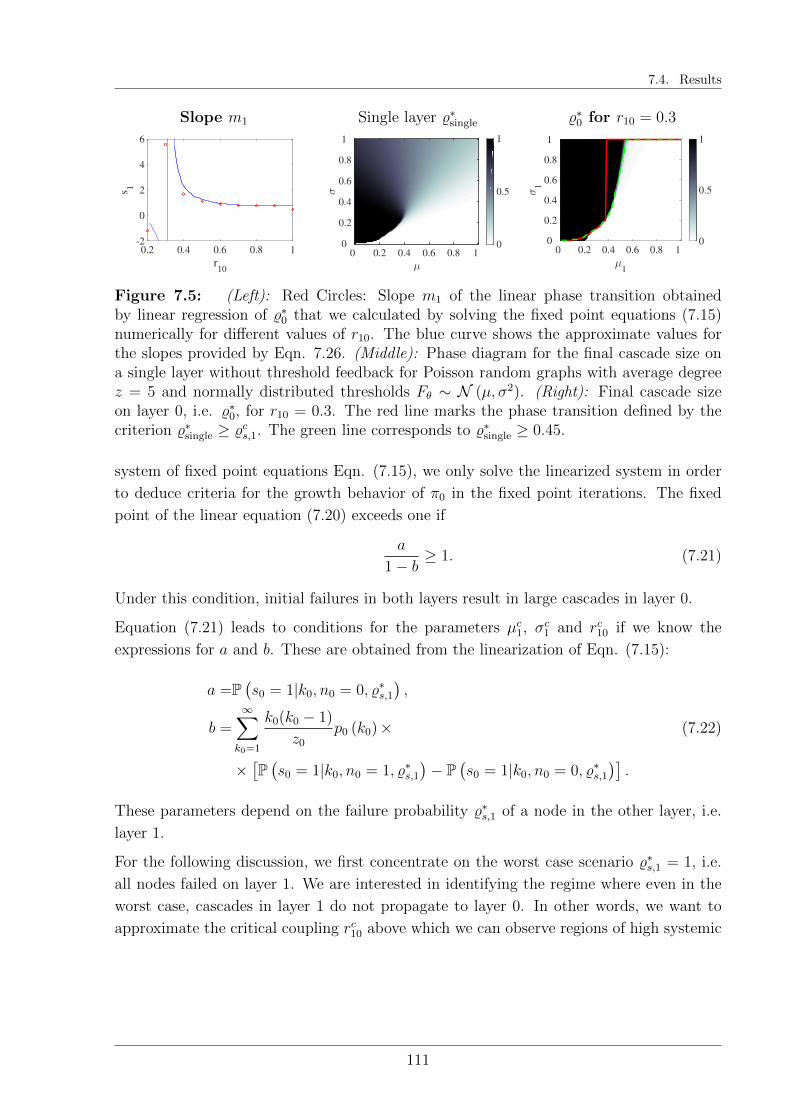
7.4. Results
Slope m1 Single layer %∗single %∗0 for r10 = 0.3
r10
0.2 0.4 0.6 0.8 1
s1
-2
0
2
4
6
µ
0 0.2 0.4 0.6 0.8 1
σ
0
0.2
0.4
0.6
0.8
1
0
0.5
1
µ1
0 0.2 0.4 0.6 0.8 1
σ1
0
0.2
0.4
0.6
0.8
1
0
0.5
1
Figure 7.5: (Left): Red Circles: Slope m1 of the linear phase transition obtainedby linear regression of %∗0 that we calculated by solving the fixed point equations (7.15)numerically for different values of r10. The blue curve shows the approximate values forthe slopes provided by Eqn. 7.26. (Middle): Phase diagram for the final cascade size ona single layer without threshold feedback for Poisson random graphs with average degreez = 5 and normally distributed thresholds Fθ ∼ N (µ, σ2). (Right): Final cascade sizeon layer 0, i.e. %∗0, for r10 = 0.3. The red line marks the phase transition defined by thecriterion %∗single ≥ %cs,1. The green line corresponds to %∗single ≥ 0.45.
system of fixed point equations Eqn. (7.15), we only solve the linearized system in order
to deduce criteria for the growth behavior of π0 in the fixed point iterations. The fixed
point of the linear equation (7.20) exceeds one if
a
1− b≥ 1. (7.21)
Under this condition, initial failures in both layers result in large cascades in layer 0.
Equation (7.21) leads to conditions for the parameters µc1, σc1 and rc10 if we know the
expressions for a and b. These are obtained from the linearization of Eqn. (7.15):
a =P(s0 = 1|k0, n0 = 0, %∗s,1
),
b =∞∑k0=1
k0(k0 − 1)
z0
p0 (k0)× (7.22)
×[P(s0 = 1|k0, n0 = 1, %∗s,1
)− P
(s0 = 1|k0, n0 = 0, %∗s,1
)].
These parameters depend on the failure probability %∗s,1 of a node in the other layer, i.e.
layer 1.
For the following discussion, we first concentrate on the worst case scenario %∗s,1 = 1, i.e.
all nodes failed on layer 1. We are interested in identifying the regime where even in the
worst case, cascades in layer 1 do not propagate to layer 0. In other words, we want to
approximate the critical coupling rc10 above which we can observe regions of high systemic
111
Chapter 7. Systemic risk in multiplex networks with asymmetric coupling and threshold feedback
risk in the left column of Fig. 7.4. With %∗s,1 = 1 the parameters a and b simplify to
a = F0(0),
b =∞∑k0=1
k0(k0 − 1)
z0
p0 (k0)
[F0
(1
k0 (1− r10)
)− F0(0)
].
(7.23)
We note that these are independent of µ1, σ1. For the set of parameters used in Fig. 7.4,
we obtain with the help of Eqn. (7.22) and Eqn. (7.21) the value of the critical coupling
rc10 = 0.204. In comparison with the numerical calculation r10 = 0.18, which takes the full
set of fixed point equations into account, this is a good approximation. That means large
cascades can propagate from layer 1 to layer 0 above a critical coupling strength rc10 ' 0.2.
This holds independently of µ1 and σ1.
Next we explain the dependence m1(r10) as shown in Fig. 7.3. By this we estimate the
slope of the phase transition line (which is of the form σ1 ∝ m1µ1). Again, we deduce
this relation from Eqs. (7.21), (7.22), but this time we cannot use %∗s,1 = 1. For %∗s,1 6= 1,
we automatically obtain a dependence on the threshold parameters µ1 and σ1 of layer 1.
Combining Eqn. (7.22) and Eqn. (7.21), we can define a critical value %cs,1 such that Eqn.
(7.21) is satisfied for %∗s,1 ≥ %cs,1:
%cs,1 :=1 + F0(0)(z0 − 1)− c0(0)
c0(r)− c0(0), (7.24)
where
c0(r) :=∞∑k0=1
k0(k0 − 1)
z0
p0 (k0)F0
(1
k0 (1− r10)
). (7.25)
This is a reformulation of Eqn. (7.21), which gives us an estimation of when to expect
large cascades in layer 0. Still, we do not know %∗s,1 without solving the full system of fixed
point equations (7.15). In the following we test two approximations for %∗s,1 which lead us
to a linear dependence between µ1 and σ1.
Case (1) The initial value %s,1(t = 0) = F1(0) = Φ (−µ1/σ1) is already enough to
determine the growth of π0 in the early stages of the fixed point iterations. Especially for
larger values of r10, a large cascade in layer 0 might be already triggered just by the initial
failures in layer 1. Therefore, we set %cs,1 ' F1(0), which results in
σ1 ∝ −µ1/Φ−1(%cs,1), (7.26)
i.e.,
m1 = −1/Φ−1(%cs,1)
(7.27)
112

7.5. Conclusions
where Φ−1 denotes the cumulative distribution function of the standard normal distri-
bution. We plot this slope using a blue line in Fig. 7.5(left), to demonstrate the good
agreement of our approximation with the numerical slopes m1 for r10 ≥ 0.4.
Case (2) For smaller coupling strengths r10 we test a second proxy for %∗s,1. A lower
bound for %∗s,1 is given by the final cascade size on a single layer %∗single, where no feedback
mechanism with another layer exists. This would coincide with %∗s,1, if layer 0 would not
exist. That means, the layer 0 cannot further amplify the failures. Cascades in single
layers have been studied in Burkholz et al. (2016a); Gleeson and Cahalane (2007). We
use their approach to plot a phase diagram for the final cascade size for Poisson random
graphs with average degree z = 5, shown in the middle panel of Fig. 7.5.
When we compare the plots of Fig. 7.3 (left) with Fig. 7.5 (middle), we observe that in
the parameter regions in Fig. 7.3 (left) where no cascades occur, also no cascades occur
in Fig. 7.5 (middle). This holds only for strong couplings r10. Consequently, in this limit,
our second approximation for %∗s,1 gives similar results as our first approximation.
However, the second case for %∗s,1, is the more general one as we can also correctly cover
the transition line for values of 0.2 ≤ µ1 ≤ 0.4. In this range, the transition line is largely
independent of the value r10. It basically coincides with the transition line for %∗single, the
fraction of failed nodes for single layer networks.
For values of µ1 larger than 0.4 and for weak coupling, e.g. for r10 = 0.3, we observe in
Fig. 7.5 (right, red line) that the transition line is no longer accurately described. The
condition %∗single ≥ %cs,1 = 0.55 gives only an upper bound for the transition line, but not
a lower one. We observe that already cascade sizes of %∗single ≥ 0.45 lead to large cascade
amplification on layer 0, due to nonlinear effects. I.e. the green dotted line in Fig. 7.5
(right) gives an almost perfect match with the numerically calculated transition line.
That means, we can even generalize our statement that the transition line for %∗single de-
termines the phase transition. This holds not only for small µ1, but also for larger µ1 and
a broad range of the coupling strength r10.
7.5 Conclusions
Our work essentially addresses the problem of whether systemic risk is increased or de-
creased if, instead of a single-layer network, a two-layer representation is used. In the
latter, the nodes of the network appear on two layers 0 and 1 with different properties.
Specifically, they have different degree distributions p0 (k0), p1 (k1) and different threshold
distributions F0 (θ0), F1 (θ1). There is an asymmetric coupling between the two layers
such that nodes that failed on layer 0 also fail on layer 1. However, nodes that did not
fail on layer 0, may still fail on layer 1 because of a cascade dynamics on layer 1. In this
113

Chapter 7. Systemic risk in multiplex networks with asymmetric coupling and threshold feedback
case, their failing threshold on layer 0 is reduced by a fraction r10, where r10 denotes the
coupling strength between the two layers.
The mutual feedback between the two layers can then result in the amplification of failure
cascades, which we study analytically. We can calculate a variable %∗l which is the final
fraction of failed nodes on each layer l ∈ 0, 1. Our measure of systemic risk is %∗ ≡ %0,
i.e. we only consider whether nodes have failed on layer 0. Obviously, if r10 is small, no
failure cascade in layer 1 can propagate to layer 0. In this case, whether or not we observe
failure cascades only depends on the conditions in layer 0. These conditions are expressed
by the parameters of the threshold distribution, µ0 and σ0, which are chosen so that no
failure cascade occurs. By varying r10, we then study the impact of failures on layer 1
on failures on layer 0. We derive an analytical approach to calculate %l, which leads to a
system of coupled fixed point equations solved numerically.
Our results are visualized through phase diagrams showing, for various parameter con-
stellations, the value of the main risk measure %∗ = %∗0. The most prominent feature is
the existence of a very sharp phase transition between a regime of no systemic risk and
a regime of full collapse. This means that small changes in the parameters µ1 and σ1,
describing the threshold distribution on layer 1, can lead to an abrupt regime shift. Our
task was then to approximate this line of transition in terms of the coupling strength r10
and the parameters of the threshold distribution. Subsequently, we use these insights to
compare the systemic risk in single-layer and two-layer networks.
The derivation of mathematical approximations for the phase transitions that are com-
pared, and confirmed, by numerical solutions of the full problem has a value on its own.
Here, we focus on the conclusions that can be made based on these calculations. First
of all, we understand that systemic risk is reduced in the two-layer network only if the
coupling strength between the two layers is rather small. Above a critical value rc10 = 0.2,
which is also estimated analytically, failures on layer 1 are amplified on layer 0 and thus
lead to an increase of the systemic risk. If we compare this with the reference case of a
single layer network, we find that the systemic risk is smaller there, for most ranges of the
parameters. Hence, above a critical coupling, it is not beneficial to split the network into
two layers, if systemic risk shall be mitigated.
Our findings are motivated by a scenario where firms have to decide whether to split
their business into a less risky core business, essential for their survival, and a subsidiary
business, which can be more risky. Such a split leads to the representation of the (same)
firm on two different levels 0 and 1, where the latter has a larger risk of failure cascades.
This decision only leads to less failure risk for the firm if the coupling between the core
business layer and the subsidiary business layer is weak enough. Close to the transition line
between the no-risk and the high-risk regime, slight changes in the firms’ failure thresholds
or in the coupling between the different businesses may potentially cause the system to
collapse completely.
114
7.5. Conclusions
There is another important conclusion to be drawn for firms that already have their
activities split between a less risky core business and a more risky subsidiary business. If
such firms estimate systemic risk based on an aggregated network representation with only
one layer instead of the two-layer representation, they may systematically underestimate
the real risk, in particular if the coupling is still strong. As we have shown, under such
conditions the systemic risk in the aggregated network is lower than in the two-layer
network. Hence, there can be drastic consequences from drawing conclusions based on an
inappropriate aggregated picture.
Closing, we would like to point out that other network properties could influence systemic
risk calculations. For example assortativity is known to affect the dynamics of a network
(D’Agostino et al., 2012; Zhou et al., 2012), and can influence the evolution of cascades
especially during crisis periods where it may vary due to network re-organization. However,
studying such influence is out of the scope of our current work, and is left for future study.
115
Chapter 8
Systemic feedback transforming
constant load cascades to effective
load redistribution
Summary
In this small interim chapter, we extend the Constant Load Exposure Diver-sification model by a simple systemic feedback mechanism. Interestingly, weobserve similar phase diagrams as for the Load Redistribution model (withoutsystemic feedback). Although these similarities can be explained analytically,the mechanisms underlying both models differ. Interventions would requireappropriately different countermeasures and therefore a good understandingof cascades on the microlevel. Comparisons of macro final cascade sizes arenot enough to identify micro-dynamics correctly.
RB wrote this chapter specifically for this thesis. RB contributed to the design of the researchquestions, derived the formulas, wrote the code and performed the analysis.
116

8.1. Introduction
8.1 Introduction
In Part I of this thesis, systemic risk originates solely from local interactions and depen-
dencies of system components. Especially in social systems, a successive downward trend
of a cascade might be observable by members of the system and prompt reactions. These
reactions can be interventions, but also a trend reinforcement, i.e. amplifications of the
cascade. As long as all system components are affected by these, we term the phenomenon
systemic feedback.
Examples for negative trend reinforcement include fire sales by distressed financial institu-
tions (Cifuentes et al., 2005) that reduce the assets’ value by all other institutions that hold
these assets. At the same time, increasing haircuts, i.e., the amount of collateral required
for a transaction, can worsen the situation (Gorton and Metrick, 2012). The common trust
in the bail-out of big institutions can have both a negative as well as a positive effect. It
might lead to excessive risk taking or prevent panics that could amplify cascades. Another
example are opinion formation cascades of binary decisions, where TV broadcasts inform
frequently about the dissemination of the opinion, for instance the percentage of voters
for a party in a poll.
In the previous chapter, the second subsidiary layer has introduced a feedback on the core
layer. From a theoretical perspective, this feedback applied to all nodes in the core layer,
as their probability increased to be connected to a failed node in the subsidiary layer.
There, we encountered already a way to deal with such a feedback analytically.
This chapter we devote to the analysis of a simple feedback mechanism that is inspired
by the previous chapter, although the feedback originates from the same layer. We show
that this extension of the CL ED model leads to similar macroscopic results as the LRD
(LLSC) model. This similarity can be explained by a comparison of the LTA calculations
and the approach on fully connected networks. Still, an observation of the macroscopic
phase diagrams would not allow us to distinguish between the two models despite the
different underlying mechanisms.
8.2 Local Tree Approximation incorporating systemic
feedback
Additional to the local interactions between network nodes in the ED model, systemic
feedback can affect the nodes’ thresholds (as in the previous chapter). The values of these
thresholds are coupled to the state of the overall system and reflect thus a degrading of
robustness in the course of a cascade.
We assume that the threshold θi(t) of each node i is proportional to the size of the func-
117
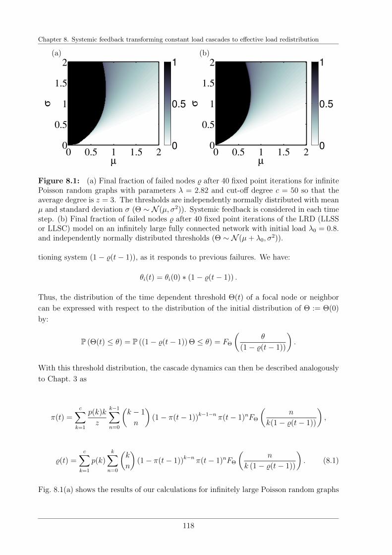
Chapter 8. Systemic feedback transforming constant load cascades to effective load redistribution
µ
σ
0 0.5 1 1.5 20
0.5
1
1.5
2
0
0.5
1
µ
σ
0 0.5 1 1.5 20
0.5
1
1.5
2
0
0.5
1
(a) (b)
Figure 8.1: (a) Final fraction of failed nodes % after 40 fixed point iterations for infinitePoisson random graphs with parameters λ = 2.82 and cut-off degree c = 50 so that theaverage degree is z = 3. The thresholds are independently normally distributed with meanµ and standard deviation σ (Θ ∼ N (µ, σ2)). Systemic feedback is considered in each timestep. (b) Final fraction of failed nodes % after 40 fixed point iterations of the LRD (LLSSor LLSC) model on an infinitely large fully connected network with initial load λ0 = 0.8.and independently normally distributed thresholds (Θ ∼ N (µ+ λ0, σ
2)).
tioning system (1− %(t− 1)), as it responds to previous failures. We have:
θi(t) = θi(0) ∗ (1− %(t− 1)) .
Thus, the distribution of the time dependent threshold Θ(t) of a focal node or neighbor
can be expressed with respect to the distribution of the initial distribution of Θ := Θ(0)
by:
P (Θ(t) ≤ θ) = P ((1− %(t− 1)) Θ ≤ θ) = FΘ
(θ
(1− %(t− 1))
).
With this threshold distribution, the cascade dynamics can then be described analogously
to Chapt. 3 as
π(t) =c∑
k=1
p(k)k
z
k−1∑n=0
(k − 1
n
)(1− π(t− 1))k−1−n π(t− 1)nFΘ
(n
k(1− %(t− 1))
),
%(t) =c∑
k=1
p(k)k∑
n=0
(k
n
)(1− π(t− 1))k−n π(t− 1)nFΘ
(n
k (1− %(t− 1))
). (8.1)
Fig. 8.1(a) shows the results of our calculations for infinitely large Poisson random graphs
118
8.3. Similarity with LRD on fully connected networks
(with average degree z = 3) as introduced in Sec. 2.4.2. Results for scale free networks
with the same average degree are almost identical. Next to it, in Fig. 8.1(b), we plot a
corresponding phase diagram for an LRD LLSC/LLSS model with initial load λ0 = 0.8
on a fully connected topology. Qualitatively, the shapes look extremely similar.
We explain this finding by an approximation of Eq. (8.1) that translates into an iterative
procedure to calculate the fraction of failed nodes for LRD models on fully connected
networks as provided by Lorenz et al. (2009).
8.3 Similarity with LRD on fully connected networks
We approximate the number of failed neighbors Nf of a node with degree k, which is
binomial distributed, in Eq. (8.1) by its average Nf ≈ kπ(t− 1) and receive
%(t) =c∑
k=1
p(k)FΘ
(kπ(t− 1)
k (1− %(t− 1))
)= FΘ
(π(t− 1)
(1− %(t− 1))
).
Assuming that the difference between the failure probability of a neighbor π(t− 1) is and
the failure probability of a node is negligible, we can substitute π(t − 1) by %(t − 1) and
arrive almost at the iterative formula
%(t) = FΘ
(λ0 +
%(t− 1)λ0
(1− %(t− 1))
),
which Lorenz et al. (2009) have derived for the (average) fraction of failed nodes in case
of LRD LLSS/LLSC cascades in an infinitely large fully connected network. If we choose
the threshold distribution for Θ according to Θ + λ0 we obtain matching results.
8.4 Discussion
We have presented an example, where the introduction of systemic feedback to a CL model
leads to a similar cascade outcome as for an LRD model without systemic feedback (on a
different network topology).
This has two implications for our perspective on the studied modeling framework.
(1) The boundaries between the different model classes are not sharp. Additional model
complexity, as for instance systemic feedback, might convert one in the other. Also several
states between a global load distribution as in case of the LRD model on fully connected
networks and a local one are possible alternatives. Similarly, several fiber bundle models
have been constructed to transfer models belong to one universality class to models in
another class (Kun et al., 2006).
119

Chapter 8. Systemic feedback transforming constant load cascades to effective load redistribution
2) Obviously, in a real world modeling approach it is not sufficient that our models match
observations of a macro state. We need further information about micro dynamics to
deduce the nature of a (cascade) process.
120
Chapter 9
Cascade size distribution for finite
networks
Summary
In the previous chapters, we have approximated the average cascade size inlarge random graphs by the cascade size in infinitely large systems. But infinite systems, large deviations from this average are very probable. We presentexplicit closed-form solutions for the full final cascade size distribution on finitefully connected and finite star-shaped networks consisting of N nodes for ageneral class of cascading processes and arbitrary threshold distributions. Withthree familiar examples from our model framework, i.e. the CL ED, the CL DDand the LRD LLSS models, we demonstrate the relevance of considering thefull probability distribution of the final cascade size, as we obtain distributionsof broad shape. Despite the high symmetry of the networks and responsefunction studied, we find surprisingly asymmetric cascade size distributions.This property persists for large networks, as the convergence of the cascade sizedistribution to a delta distribution is relatively slow. This finding questionsthe average as suitable risk measure.
Based on R. Burkholz, F. Schweitzer, and H. Herrmann, “Cascade size distribution for finite net-works”. Working Paper. RB contributed to the design of the research questions and to discussions. RBderived the formulas. RB analyzed and interpreted the results. RB wrote the first draft of the manuscript.
121
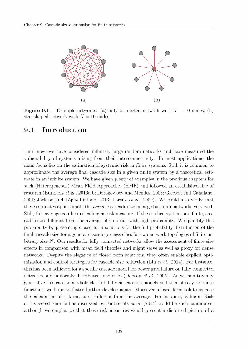
Chapter 9. Cascade size distribution for finite networks
(a) (b)
Figure 9.1: Example networks: (a) fully connected network with N = 10 nodes, (b)star-shaped network with N = 10 nodes.
9.1 Introduction
Until now, we have considered infinitely large random networks and have measured the
vulnerability of systems arising from their interconnectivity. In most applications, the
main focus lies on the estimation of systemic risk in finite systems. Still, it is common to
approximate the average final cascade size in a given finite system by a theoretical esti-
mate in an infinite system. We have given plenty of examples in the previous chapters for
such (Heterogeneous) Mean Field Approaches (HMF) and followed an established line of
research (Burkholz et al., 2016a,b; Dorogovtsev and Mendes, 2003; Gleeson and Cahalane,
2007; Jackson and Lopez-Pintado, 2013; Lorenz et al., 2009). We could also verify that
these estimates approximate the average cascade size in large but finite networks very well.
Still, this average can be misleading as risk measure. If the studied systems are finite, cas-
cade sizes different from the average often occur with high probability. We quantify this
probability by presenting closed form solutions for the full probability distribution of the
final cascade size for a general cascade process class for two network topologies of finite ar-
bitrary size N . Our results for fully connected networks allow the assessment of finite size
effects in comparison with mean field theories and might serve as well as proxy for dense
networks. Despite the elegance of closed form solutions, they often enable explicit opti-
mization and control strategies for cascade size reduction (Liu et al., 2014). For instance,
this has been achieved for a specific cascade model for power grid failure on fully connected
networks and uniformly distributed load sizes (Dobson et al., 2005). As we non-trivially
generalize this case to a whole class of different cascade models and to arbitrary response
functions, we hope to foster further developments. Moreover, closed form solutions ease
the calculation of risk measures different from the average. For instance, Value at Risk
or Expected Shortfall as discussed by Embrechts et al. (2014) could be such candidates,
although we emphasize that these risk measures would present a distorted picture of a
122
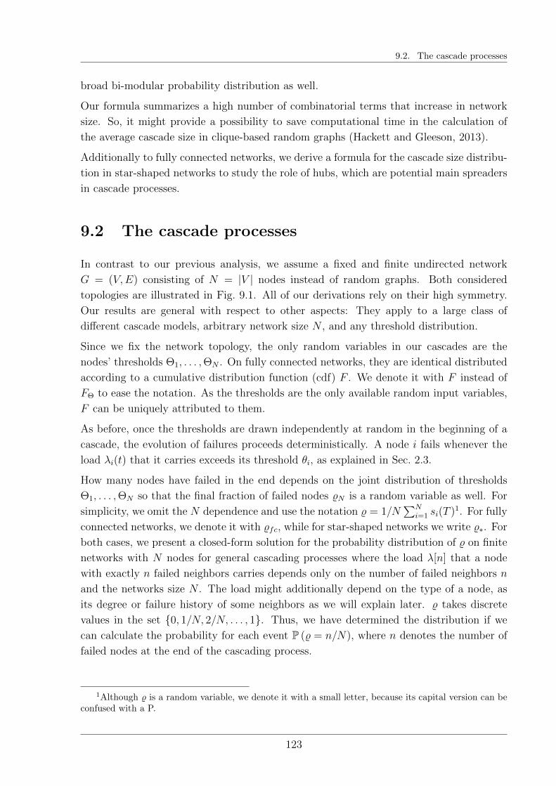
9.2. The cascade processes
broad bi-modular probability distribution as well.
Our formula summarizes a high number of combinatorial terms that increase in network
size. So, it might provide a possibility to save computational time in the calculation of
the average cascade size in clique-based random graphs (Hackett and Gleeson, 2013).
Additionally to fully connected networks, we derive a formula for the cascade size distribu-
tion in star-shaped networks to study the role of hubs, which are potential main spreaders
in cascade processes.
9.2 The cascade processes
In contrast to our previous analysis, we assume a fixed and finite undirected network
G = (V,E) consisting of N = |V | nodes instead of random graphs. Both considered
topologies are illustrated in Fig. 9.1. All of our derivations rely on their high symmetry.
Our results are general with respect to other aspects: They apply to a large class of
different cascade models, arbitrary network size N , and any threshold distribution.
Since we fix the network topology, the only random variables in our cascades are the
nodes’ thresholds Θ1, . . . ,ΘN . On fully connected networks, they are identical distributed
according to a cumulative distribution function (cdf) F . We denote it with F instead of
FΘ to ease the notation. As the thresholds are the only available random input variables,
F can be uniquely attributed to them.
As before, once the thresholds are drawn independently at random in the beginning of a
cascade, the evolution of failures proceeds deterministically. A node i fails whenever the
load λi(t) that it carries exceeds its threshold θi, as explained in Sec. 2.3.
How many nodes have failed in the end depends on the joint distribution of thresholds
Θ1, . . . ,ΘN so that the final fraction of failed nodes %N is a random variable as well. For
simplicity, we omit the N dependence and use the notation % = 1/N∑N
i=1 si(T )1. For fully
connected networks, we denote it with %fc, while for star-shaped networks we write %∗. For
both cases, we present a closed-form solution for the probability distribution of % on finite
networks with N nodes for general cascading processes where the load λ[n] that a node
with exactly n failed neighbors carries depends only on the number of failed neighbors n
and the networks size N . The load might additionally depend on the type of a node, as
its degree or failure history of some neighbors as we will explain later. % takes discrete
values in the set 0, 1/N, 2/N, . . . , 1. Thus, we have determined the distribution if we
can calculate the probability for each event P (% = n/N), where n denotes the number of
failed nodes at the end of the cascading process.
1Although % is a random variable, we denote it with a small letter, because its capital version can beconfused with a P.
123
Chapter 9. Cascade size distribution for finite networks
9.3 Cascade size distribution on fully connected net-
works
We offer two different representations of the final cascade size distribution for fully con-
nected networks: one that enumerates all possible combinations of failures that could have
led to a cascade outcome, and one which can be deduced by the inclusion-exclusion princi-
ple and whose implementation requires less computational resources. Both representations
rely on combinatorial arguments, which we explain next. First, we note that each non-
failed node in the network is exactly in the same state. They all have the same degree,
the same neighbors and carry the same load λ[n], if n other nodes have failed already.
If %fc = n/N is the final cascade outcome we know that all surviving N − n nodes must
have thresholds larger than this load λ[n]. The probability for this event is
N−n∏i=1
P (Θi > λ[n]) = (1− F (λ[n]))N−n ,
since we assume that the thresholds are independently distributed. There are(Nn
)different
combinations of n surviving nodes out of the total N nodes. The remaining n nodes fail
altogether with a probability pn that needs to be determined. In summary, we can write
the cascade distribution as:
P(%fc =
n
N
)=
(N
n
)(1− F (λ[n]))N−n pn. (9.1)
The probability pn that all n of the remaining nodes fail is equivalent to the failure of
all nodes in a network with n nodes, since non-failed nodes do not influence the amount
of load that any of the n nodes carries. The load required to cause a node to fail is
determined by the node’s threshold, while the entire configuration of all thresholds defines
the order of the nodes’ failure. But not all threshold configurations lead to n failures. For
instance, it is not enough that all n nodes have a threshold smaller than λ[k]. If each
node has a threshold Θ > λ0, no node fails initially and the cascade cannot start. In each
time step, enough failures need to occur to trigger new failures. This can be translated
into a criterion that identifies the threshold configurations that lead to exactly k failures.
Whenever a node’s threshold lies in the interval (λ[j − 1], λ[j]], it fails after j nodes have
failed before (with j = 1, . . . , N − 1). We denote the number of nodes with this property
with mj. All m0 nodes with threshold in (−∞, λ[0]] fail initially, while all mN nodes
with thresholds in (λ[N − 1],∞] never fail. This definition implies that all nodes with a
threshold corresponding to mj fail before or at the same time as the nodes corresponding
to ml, if l > j, since λ[l] > λ[j]. Each possible threshold configuration translates into a
vector mN = (m0, . . . ,mN). In the first cascade time step, all m0 nodes fail. We require
124
9.3. Cascade size distribution on fully connected networks
m0 > 0, otherwise nothing happens. In the second time step, all nodes fail whose failure
premises at least m0 failed neighbors. This includes all nodes that correspond to m1. In
order to cause the failures of at least all nodes that belong to m2 (or any j > 2), the total
number of failures before (or at the same time) m0 +m1 needs to be at least 2. Continuing
this argument, for each j = 1, . . . , n − 1 we require mj ≥ j + 1 −∑j−1
l=0 ml and in total∑n−1l=0 ml = n. We define the set of all such causal configurations for a cascade of size n/N
as
In :=
mn−1 ∈ 0, . . . , nn
∣∣ j∑l=0
ml ≥ j + 1 (∀j ∈ 0, . . . , n− 2),n−1∑l=0
ml = n
and sum the probabilities of all those configurations in order to calculate pn. Since each
node’s threshold lies in the interval (λ[j − 1], λ[j]] with probability F (λ[j])−F (λ[j − 1]),
we have
pn =∑m∈In
n!∏n−1j=0 (mj!)
F (λ[0])m0
n−1∏j=1
(F (λ[j])− F (λ[j − 1]))mj .
The enumeration of all configurations in In is computationally very expensive, and the
summation of mostly small summands numerically inaccurate. But we can derive an
iterative formula for pn with the help of the probabilistic inclusion-exclusion principle
(Szpankowski, 2001):
pn =n−1∑l=0
(−1)n+l+1
(n
l
)F (λ[l])n−l pl, (9.2)
l = 2, . . . , N with p0 = 1, p1 = F (λ[0]). A proof is given in Appendix B.
9.3.1 Model examples on fully connected networks
Constant load models
As first example, we calculate the cascade size distributions for the ED model as introduced
in Sec. 2.3.1, which has been well studied on infinite configuration type random graphs
(Burkholz et al., 2016a; Dodds and Payne, 2009; Gleeson and Cahalane, 2007; Hurd and
Gleeson, 2013). We recall that it coincides with the DD model on fully connected networks.
Each node carries the fraction of its failed neighbors as load. In a fully connected network
with N nodes, every node has N − 1 neighbors and consequently carries the load λ[n] :=
n/(N − 1), if n neighbors have failed. The average final cascade size on infinite fully
connected networks has already been calculated by Lorenz et al. (2009). However, Fig.
9.2 (a) reveals that the average is not an appropriate risk measure on finite networks,
125

Chapter 9. Cascade size distribution for finite networks
0.00
0.02
0.04
0.06
0.00 0.25 0.50 0.75 1.00ρfc
P
σ 0.40.50.60.71
0.00
0.05
0.10
0.15
0.20
0.00 0.25 0.50 0.75 1.00ρfc
P
(µ,σ) (5,5)(1,5)(0.5,0.3)(1,1)(0.5,5)
(a) (b)
Figure 9.2: Distribution of the fraction of failed nodes %fc on a fully connected networkwith normally distributed thresholds with mean µ + λ0 and standard deviation σ (i.e.Θ ∼ N (0.5 + λ0, σ
2)) for the (a) ED model with N = 50 nodes and inital load λ0 = 0,and (b) fiber bundle model with N = 30 nodes and inital load λ0 = 1.
since the distribution can be broad and even of bi-modular shape. Thus, it would be
misleading to expect a cascade size outcome that is similar to the average. Fig. 9.2 (a)
shows the cascade size distribution for N = 50 nodes and normally distributed thresholds
with mean µ = 0.5 and different standard deviations σ. The network and the threshold
distribution are highly symmetric so that the nodes are very similar. Thus, it is surprising
that the cascade size distribution is of such asymmetric and broadly distributed shape (see
parameters σ = 0.4 and σ = 0.5 in Fig. 9.2 (a)). For decreasing σ, the peak at a value close
to 0 increases, while the smaller peak close to 1 decreases until the latter one completely
vanishes. For σ ≤ 0.1, no node fails (%fc = 0) with high probability. For increasing σ,
the two peaks of the cascade size distribution move closer together, overlap and merge
to a single peak at %fc = 0.5 for σ ≥ 0.7. This leads to an axisymmetric distribution
around %fc = 0.5, as expected. The peak becomes more pronounced for increasing σ as
the standard deviation of the cascade size distribution decreases. Still, for most parameter
values it is important to take the whole cascade size distribution into account rather than
focusing on its average to assess the cascade risk correctly.
For increasing network size N , the distribution converges to a point measure, whose value
has been calculated by Lorenz et al. (2009). The speed of this convergence decides if the
presented phenomena are just an artifact of rather small networks or can be observed in
for realistic network sizes relevant for applications.
126
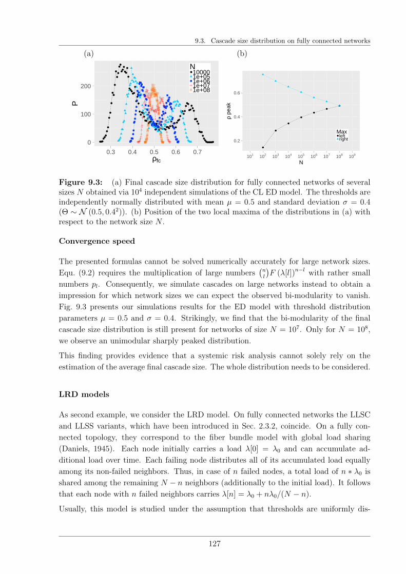
9.3. Cascade size distribution on fully connected networks
0
100
200
0.3 0.4 0.5 0.6 0.7ρfc
PN 100001e+051e+061e+071e+08
0.2
0.4
0.6
101 102 103 104 105 106 107 108 109
N
ρ pe
ak
Max leftright
(a) (b)
Figure 9.3: (a) Final cascade size distribution for fully connected networks of severalsizes N obtained via 104 independent simulations of the CL ED model. The thresholds areindependently normally distributed with mean µ = 0.5 and standard deviation σ = 0.4(Θ ∼ N (0.5, 0.42)). (b) Position of the two local maxima of the distributions in (a) withrespect to the network size N .
Convergence speed
The presented formulas cannot be solved numerically accurately for large network sizes.
Equ. (9.2) requires the multiplication of large numbers(nl
)F (λ[l])n−l with rather small
numbers pl. Consequently, we simulate cascades on large networks instead to obtain a
impression for which network sizes we can expect the observed bi-modularity to vanish.
Fig. 9.3 presents our simulations results for the ED model with threshold distribution
parameters µ = 0.5 and σ = 0.4. Strikingly, we find that the bi-modularity of the final
cascade size distribution is still present for networks of size N = 107. Only for N = 108,
we observe an unimodular sharply peaked distribution.
This finding provides evidence that a systemic risk analysis cannot solely rely on the
estimation of the average final cascade size. The whole distribution needs to be considered.
LRD models
As second example, we consider the LRD model. On fully connected networks the LLSC
and LLSS variants, which have been introduced in Sec. 2.3.2, coincide. On a fully con-
nected topology, they correspond to the fiber bundle model with global load sharing
(Daniels, 1945). Each node initially carries a load λ[0] = λ0 and can accumulate ad-
ditional load over time. Each failing node distributes all of its accumulated load equally
among its non-failed neighbors. Thus, in case of n failed nodes, a total load of n ∗ λ0 is
shared among the remaining N − n neighbors (additionally to the initial load). It follows
that each node with n failed neighbors carries λ[n] = λ0 + nλ0/(N − n).
Usually, this model is studied under the assumption that thresholds are uniformly dis-
127

Chapter 9. Cascade size distribution for finite networks
tributed and a single node fails initially. This node distributes a load L0 to the remaining
N functional network neighbor at time t = 1. (We consider a network of size N + 1 for
simplicity.) By defining the initial load as λ0 = L0/N and uniformly distributed thresh-
olds Θ ∼ Unif[0, 1], our approach at time t = 0 matches the described setting at t = 1.
Consequently, the final cascade size distribution coincide in the end. For the special (and
simplifying) case of uniformly distributed thresholds, a formula for the final cascade size
distribution has been derived by (Dobson et al., 2005).
In our framework analysis, we focus on normally distributed thresholds instead. The final
cascade size distribution for this case is shown in Fig. 9.2 (b). Again we find broad
distributions. Noticeably, a total break down of the network (%fc = 1) often occurs with
a much higher probability than slightly smaller final cascade sizes. There seems to be a
tendency towards complete failure in the system if a certain cascade size is reached and
high load is accumulated.
OLRD models
In case of OLRD models, we face the additional obstacle that the load λ[n] that a node
with n failed neighbors carries depends on the thresholds of the nodes that have failed
before. Consequently, λ[n] is a random variable Λ[n] that is defined by
Λ[n] =
∑ni=1−Θi
N − n
conditional on the fact that Θi ≤ 0. So, it depends on the whole history of the cascade
process. Unfortunately, the inclusion-exclusion does not hold in such a case and our
derivations do not apply to OLRD models.
At this point, we can formulate the cascade size distribution only as multi-dimensional
integral over all possible threshold configurations. The result is not practically computable.
9.4 Final cascade size distribution on star-shaped net-
works
Next, we shift our focus to a finite star-shaped network consisting of N nodes as illustrated
in Fig. 9.1 (b). This is the simplest possible topology where a hub and leaves are present.
In fact, we only have two categories of nodes, the single hub in the center with high degree
d = N − 1, and N − 1 leaf nodes, i.e., the nodes with degree 1. Under the constraint that
all nodes in a network are part of a single connected component, a star is the topology that
minimizes the overall connectivity (and thus the total number of links). Consequently, we
would expect relatively small systemic risk, since the low connectivity hinders cascades to
128
9.4. Final cascade size distribution on star-shaped networks
proceed further in time. We discuss later, if this intuition really applies.
A cascade ends after maximally three time steps. The central node has a prominent role,
as it is the only node in the network that can further distribute accumulated load. Initial
failures might happen at t = 0 before the central node fails (among other nodes) at t = 1,
and this failure possibly causes neighboring nodes to fail at t = 2. If the center does not
fail, initial failures cannot become further amplified and the cascade stops after t = 0. If
the center fails initially, it can cause further failures at t = 1, but then the cascade stops.
Because of the limited number of possibilities, we can take the history of the center into
account when we formulate a closed-form solution for the distribution of the final cascade
size %∗ for general cascading processes.
We allow the central node’s cdf Fc and load λc to be different from a leaf node’s cdf F and
its load λl. As before, we assume that the load λc[n] that the center carries only depends
on the number of its failed neighbors n (and the network size N). A leaf node can fail
initially with probability F (λl[0]) (with 0 neighboring failures) or, if the center has failed
before, it can carry the load λl[1, j, l], which depends on two additional variables that are
determined by the history of the center. j denotes the number of failed leaf nodes that
have distributed load to the center, before the center has failed. l indicates the number of
nodes among which the accumulated load of the center is shared (when the center fails).
We simply add the probabilities for all different cases and obtain:
P(%∗ =
n
N
)= (1− Fc (λc[n]))
(N − 1
n
)F (λl[0])n (1− F (λl[0]))N−1−n
+ Fc(λc[0])
(N − 1
n− 1
) n−1∑j=0
(n− 1
j
)F (λl[0])j
× (F (λl[1, 0, N − 1− j])− F (λl[0]))n−1−j (1− F (λl[1, 0, N − 1− j]))N−n
+
(N − 1
n− 1
) n−1∑j=1
(n− 1
j
)F (λl[0])j (Fc (λc[j])− Fc (λ[0]))
× (F (λl[1, j, N − 1− j])− F (λl[0]))n−1−j (1− F (λl[1, j, N − 1− j]))N−n .(9.3)
The first summand considers the case when the center does not fail, while the second term
adds the probability for the case when the center fails initially. Then, each of the other
n − 1 failures of leaves can either occur initially or because of a load distribution by the
center. The size of this load might depend on the number of nodes l that fail initially
together with the center, since these nodes cannot receive load after the failure of the
center. The index j in the third term finally takes the events into account when j leaves
have failed before the center.
Even though each cascade is over after maximally three time steps, the final cascade size
129
Chapter 9. Cascade size distribution for finite networks
can still be large if enough load is distributed by the center. Thus, low interconnectivity
is not necessarily an advantage. Here, load can be distributed almost globally to network
neighbors, a familiar problem in case of the failure of hubs. The small number of times
steps in the cascade evolution additionally make interventions more difficult, because these
need to be implemented fast.
Still, we expect that systemic risk is low in some of our cascade model examples that
reduce the impact of the failure of hubs.
9.4.1 Model examples on star-shaped networks
ED models
In Equ. (9.3), the loads are defined as λl[0] = λc[0] = 0, λl[1, j, l] = 1 and λc[j] = j/(N−1)
for all values of j and l in case of an ED model. We would expect a bi-modular cascade
size distribution because of the prominent role of the central node. If the center can
withstand the failure of some of its neighbors, the cascade stops early without causing
high damage with high probability. But if the center fails, the further failure of leaves
might be amplified, because they need to carry a higher load. Each event, the survival
and the failure of the center, account for one peak in the cascade size distribution.
Fig. 9.4 (a) confirms this intuition for most cases. The plot shows the final cascade size
distribution for normally distributed thresholds with parameters µ = 0.5 and different
standard deviations σ. For all σ ≤ 3, we observe a bi-modular distribution whose left
peak is higher than the right. These peaks move closer together towards 0.5 and merge
to a single peak for σ = 4. Although intuitively convincing, the bi-modular shape of
the distribution relies crucially on the size of the load distribution mechanism of the ED
model. We compare these results with the DD model where damage is diversified.
DD models
In DD models the loss, the failure of hubs inflict, is reduced. It has been introduced in
Lorenz et al. (2009) and contrasted with the ED model on configuration model random
graphs in Burkholz et al. (2016a). Each failing node distributes a total load of 1 equally
among its network neighbors. While the model coincides with the ED model on fully con-
nected networks, for star-shape networks we have λl[1, j, l] = 1/(N−1) and λc[j] = j again
for all values of j and l. Here, the center fails with high probability, but this failure does
not cause significant further damage. Because of this, we only observe unimodular cascade
size distributions in Fig. 9.4 (b). Generally, the cascade risk is reduced in comparison
with the ED model.
130

9.4. Final cascade size distribution on star-shaped networks
0.00
0.05
0.10
0.15
0.00 0.25 0.50 0.75 1.00ρ*
P
σ 0.40.50.824
0.00
0.05
0.10
0.15
0.00 0.25 0.50 0.75 1.00ρ*
P
σ 0.40.50.824
(a) (b)
Figure 9.4: Distribution of the fraction of failed nodes %∗ on a star-shaped networkwith N = 50 nodes for the (a) ED model and (b) DD model. The thresholds are normallydistributed with mean µ = 0.5 and standard deviation σ (i.e. Θ ∼ N (0.5, σ2). The initialload is λ0 = 0.
Systemic risk reduction in CL models
In both Constant Load models, systemic risk could be further reduced by providing the
center with high thresholds. Similar to our findings in Chapt. 4, it costs less resources to
increase the threshold of the center in case of ED. We would only need to ensure that the
maximal load λc = 1 cannot exceed the threshold Θc. In contrast, the maximal load that
the central node can carry is N −1 in a DD model. Instead, the (N −1) leaf nodes can be
cost effectively protected, as each only needs to withstand a maximal load of 1/(N − 1).
Thus, ED and DD models on star-shaped topologies could be sheltered effectively from
systemic risk.
Still, we note a difference between the two models that we have not paid attention to yet.
The connectivity of the system at the end of a cascade is not relevant for our notion of
systemic risk, although it might be essential for system performance. From this perspec-
tive, the DD model can be quite problematic, as the center fails with high probability and
the network becomes disconnected. If this corresponds to a short shut-down in a crisis
and connections can be easily established afterwards, the DD model weights might still
represent a good system design option.
LRD models
Our third example it the LRD LLSS model, i.e. the fiber bundle model (now with a
form of local load sharing). We need to take the two additional parameters j and l into
account, as they define the amount of load that the center accumulates before it distributes
131
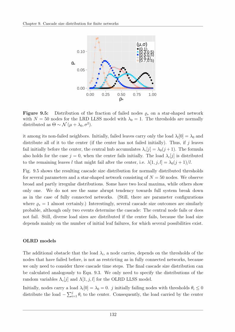
Chapter 9. Cascade size distribution for finite networks
0.00
0.05
0.10
0.00 0.25 0.50 0.75 1.00ρ*
P
(µ,σ) (0,1)(0.3,0.5)(0.5,0.5)(0.5,1)(0.7,0.5)
Figure 9.5: Distribution of the fraction of failed nodes %∗ on a star-shaped networkwith N = 50 nodes for the LRD LLSS model with λ0 = 1. The thresholds are normallydistributed as Θ ∼ N (µ+ λ0, σ
2).
it among its non-failed neighbors. Initially, failed leaves carry only the load λl[0] = λ0 and
distribute all of it to the center (if the center has not failed initially). Thus, if j leaves
fail initially before the center, the central hub accumulates λc[j] = λ0(j+ 1). The formula
also holds for the case j = 0, when the center fails initially. The load λc[j] is distributed
to the remaining leaves l that might fail after the center, i.e. λ[1, j, l] = λ0(j + 1)/l.
Fig. 9.5 shows the resulting cascade size distribution for normally distributed thresholds
for several parameters and a star-shaped network consisting of N = 50 nodes. We observe
broad and partly irregular distributions. Some have two local maxima, while others show
only one. We do not see the same abrupt tendency towards full system break down
as in the case of fully connected networks. (Still, there are parameter configurations
where %∗ = 1 almost certainly.) Interestingly, several cascade size outcomes are similarly
probable, although only two events determine the cascade: The central node fails or does
not fail. Still, diverse load sizes are distributed if the center fails, because the load size
depends mainly on the number of initial leaf failures, for which several possibilities exist.
OLRD models
The additional obstacle that the load λi, a node carries, depends on the thresholds of the
nodes that have failed before, is not as restricting as in fully connected networks, because
we only need to consider three cascade time steps. The final cascade size distribution can
be calculated analogously to Equ. 9.3. We only need to specify the distributions of the
random variables Λc[j] and Λ[1, j, l] for the OLRD LLSS model.
Initially, nodes carry a load λl[0] = λ0 = 0. j initially failing nodes with thresholds θi ≤ 0
distribute the load −∑j
i=1 θi to the center. Consequently, the load carried by the center
132
9.4. Final cascade size distribution on star-shaped networks
is distributed as
Λc[j] = −j∑i=1
Θfi
where Θfi denotes the random threshold of a node conditional on its initial failure, i.e.
Θi ≤ 0. It simplifies our calculations, if we consider instead of the pdf of Λc[j] a distribution
that is not conditional on the failure of the nodes i. This distribution is not a probability
distribution. Because of this, we denote it by dΛc[j]. It sums up the probability mass of
all threshold configurations, where j nodes have thresholds smaller than zero.
Let’s assume that each threshold distribution has a density pΘ or pc for the central node.
dΛc[j] can then be written as convolution dΛc[j] = d∗jΘ (z) where dΘ is defined by
dΘ(x) := pΘ(−x), if x ≥ 0, and dΘ(x) := 0, if x < 0.
Similarly, the load Λ[1, j, l] that leave nodes receive at time t = 2 after j nodes have failed
initially and triggered the failure of the center, is distributed as
Λ[1, j, l] =−Θf
c −∑j
i=1 Θfi
l
where Θfi follow the distribution of Θi conditional on Θi ≤ 0 and Θf
c follows the distribution
of Θc conditional on 0 ≤ Θc ≤ −∑j
i=1 Θfi . Again, we define a density dΛ[1,j,l] as
dΛ[1,j,l](z) :=
∫ ∞zl
pc(x− zl)dΛc[j](x) dx
for z ≥ 0. This is the probability that a threshold configuration of j initially failing nodes
and a central node leads leads to the distribution of the load z to the remaining l nodes
(unconditional on all mentioned failures).
With these definitions we can adapt Equ. 9.3 for the OLRD LLSS model to
P(%∗ =
n
N
)=
(N − 1
n
)(1− F (0))N−1−n
∫ ∞0
(1− Fc (x)) dΛc[n](x) dx
+
(N − 1
n− 1
) n−1∑j=0
(n− 1
j
)∫ 0
−∞(F (−y)− F (0))n−1−j (1− F (−y))N−n pc(y) dy
+
(N − 1
n− 1
) n−1∑j=1
(n− 1
j
)∫ ∞0
(F (z)− F (0))n−1−j
× (1− F (z))N−n dΛ[1,j,N−1−j](z) dz.
As the numerical calculation of the given formula is more involved (although possible), we
133
Chapter 9. Cascade size distribution for finite networks
omit the discussion of examples.
9.5 Conclusions
In summary, we have presented closed-form solutions for the cascade size probability dis-
tribution corresponding to a general class of cascade models on fully connected and star-
shaped networks with respect to an arbitrary threshold distribution. Fully connected
networks are especially of interest as a proxy for dense networks, while stars are suitable
for investigating the role of hubs.
With our derivations, we have gained further insights into the microscopic evolution in time
of a cascading process. In finite networks, neighbors of a node do not fail independently.
The failure of each node depends on the specific threshold configuration, and is thus
determined regarding all other threshold values.
We have seen in Chapt. 4 that these threshold configurations and the studied cascade model
influence the time until a cascade reaches its steady state. Moreover, the example of a star-
shaped network has led us to the insight that the presence of hubs can not only amplify,
but also accelerate or block cascades, when they represent channels connecting otherwise
disconnected network components. Such fast cascade evolutions can be problematic for
the implementation of interventions.
Our results allow further studies of final cascade size distributions with respect to various
shapes of the threshold distribution, but also to the network size N . Furthermore, explicit
formulas can enable the optimization of several parameters for the design of robust systems
and invite the treatment of model expansions like restorations as in Liu et al. (2014).
Most importantly, we have shown for the CL ED, CL DD and LRD LLSS models that a
good risk assessment in finite systems of finite size N demands the consideration of full
cascade size distributions. Bi-modular distributions can occur even in large networks, for
instance, in the order of magnitude of N = 107 nodes.
With our examples, we hope to encourage the further study of full cascade size distributions
on finite networks.
134
“The goal is to turn data into information, and information into insight.”
Carly Fiorina
Part III
Modeling systemic risk in a data
driven approach
135

Introduction: Systemic risk and international trade of staple food
Introduction: Systemic risk and
international trade of staple food
In Part I of this thesis, we have investigated generic models for cascade processes under
network uncertainty. Then, in Part II, we have critically reflected on our assumptions
and successively introduced further complexity to our models. Two sources of feedback,
one originating from another network layer, another originating from the system response
to the cascade evolution, have been discussed. Moreover, we have emphasized the high
variation of the final cascade size that finite systems can exhibit. All these three aspects,
the feedback between multiplex layers, systemic feedback by variables on the macro level,
and system finiteness are of high relevance also in Part III.
However, in Part III, we successively shift our perspective from generic models to an
Overload Redistribution cascade model that we motivate by observed data and that we
adjust to our modeling purpose. This allows us to transfer some of our insights to an
application context.
In general, the high amount of variables in our models, which need to be inferred from
data, pose a practical challenge. For each network node, a failure threshold needs to be
determined, and, for each link, a load that is transfered in case of the failure of one node
needs to be defined. Our choice is simplified by an economic motivation of these variables.
In fact, they can be defined by measurable quantities.
In Part III, we study the international trade of the four major internationally traded
staples: maize (also known as corn), rice, soy, and wheat. While we interpret the world’s
countries as nodes in an international trade network, weighted links represent aggregated
trades of a specific crop in a given year between two countries. We specify in Chapter
10 how we obtain such networks from a dataset provided by the Food and Agriculture
Organisation of the United Nations (FAO) for the public.2
These networks contain information about the dependence of countries on the international
market and about economic relationships between countries with respect to staple foods.
The trade relationships result from economic mechanisms matching supply and demand
2http://faostat3.fao.org/home/E
137
Chapter 9. Introduction: Systemic risk and international trade of staple food
in a given year. Thus, they determine the availability of food on the country level and are
therefore an important factor for efforts to ensure food security. The FAO defines food
security as a “situation that exists when all people, at all times, have physical, social, and
economic access to sufficient, safe, and nutritious food that meets their dietary needs and
food preferences for an active and healthy life” (Food Agriculture Organization, 2001).
We focus on the aspect of stability in the following chapters and study the fragility of the
trade network with respect to shocks.
There is a wide range of risk factors for agricultural production. Especially in the course of
climate change, weather conditions are expected to become more extreme and can pose a
challenge to agricultural production (Schmidhuber and Tubiello, 2007). Crops are sensitive
to extreme temperatures, droughts or floods put yields at risk (Puma et al., 2015, and
references therein), and water famine can hamper irrigation (Misra, 2014). The decline
of global pollinators additionally challenges agricultural production (Potts et al., 2010).
Also crop pests and pathogens can reduce yields (Garrett, 2013), while local political
instabilities and wars might hinder farming. The list of possible shocks on the production
side can be continued (Puma et al., 2015; Rosegrant and Cline, 2003).
Additional to that, shocks on the demand side can lead to a reorganization of the trade
network. New crop usage possibilities, as for instance, biofuel production (Mitchel, 2008;
Zilberman et al., 2012), or increases for the demand of feed for meat production might
compete with human consumption of crops and increase the total demand (Spiertz and
Ewert, 2009, and references therein). Also the increasing demand due to population growth
is of concern and might influence the export behavior of food producing countries (Suweis
et al., 2015). Although such demand increases might not occur immediately, also more
gradual changes lead to trade reorganizations.
Price adjustments are the results of such changes in production and demand and influence
the future evolution of the food system. Moreover, rapid price changes might refer to
additional speculation effects (Lagi et al., 2015, and references therein). Food prices and
their variability are an important indicator for food security, as they determine the food
consumption options of the poorest and impact the profitability of agricultural production.
Food prices provide an orientation for market participants and are thus not only a result
of economic interactions, but are also a source of systemic feedback.
We return to the special role of prices in Chap. 12, when we introduce a more refined
cascade model that incorporates price dynamics.
First and foremost, we are interested in the reorganization of the international trade
network in response to shocks on the production or demand side. While the causes of
such shocks can be manifold and require careful modeling, we make simple assumptions
about the size of the shocks and study several scenarios that have the purpose to reveal
the dependency structure between countries. Our focus lies on the response of the system
138
Introduction: Systemic risk and international trade of staple food
to shocks and cascading readjustment of trade links.
Such cascading phenomena have been termed multiplier effect (Giordani et al., 2014)
among others. Although its relevance has been acknowledged (Giordani et al., 2014; Puma
et al., 2015), to our knowledge, it has been neglected in resilience analyses of international
food trade networks (Puma et al., 2015; Suweis et al., 2015; Wu and Guclu, 2013).
In Chap. 11, we first study the effect of cascading export reductions as response of shocked
countries that propagate through a trade network according to a simple variant of an
overload redistribution cascade model. Ref. (Giordani et al., 2014) provides evidence that
national export bans and protective market behavior (including subsidies and other trade
policies) can be observed and impact food prices. How exactly these export bans influence
international trade is subject to different risk scenarios. In Ref. (Puma et al., 2015),
shocked countries discard completely their exports and reallocate oversupplies according
to a GDP ranking of possible trade partners. This is an extreme shock scenario and does
not encounter several cascade steps.
In contrast, we study distortions of the system as response to relatively small initial shocks
and still preserve basic trade relationships. Our approach has the advantage that many
of the mechanisms that have formed the trade networks under study are still reflected in
our model. Moreover, in Chap. 12, we extend our generic cascade model to incorporate
further observed trade characteristics and include systemic feedback in form of evolving
food prices.
Furthermore, we introduce a multiplex perspective, as we consider maize, rice, soy and
wheat trade. All of these networks are coupled, as they can substitute each other to
a certain degree. For instance, rising maize prices make soy more attractive as feed in
comparison to maize and vice versa. Also people with a preference for rice as staple crop
might consider to eat wheat instead, if rice prices grow exorbitantly. Because of this, crop
prices and thus also the corresponding trade dynamics are strongly coupled. Before we
acknowledge this coupling, we start with an exploration of the studied data sets and treat
them as separate in our simple OLRD cascade model.
As preparation, we first give an overview of the studied datasets and present a descriptive
data analysis in the next chapter.
139

Chapter 10
International trade of staple food: A
descriptive data analysis
Summary
We interpret the annual international trade of maize, rice, soy, and wheat asfour different temporal weighted networks and compare their basic properties.In this regard, we identify the main economic actors and discuss the evolutionof major trade relationships. This supports our understanding of the systemand forms our intuition for later improvement of our cascade models. For thispurpose, our main observations concern the overall connectivity of the net-works and the heterogeneity of the dependencies. We find that the numberof participants in trade as well as the interconnectivity of the networks growover time for all considered staples. While this can be interpreted as increasingmarket integration, the high dissimilarity of trade volumes suggests still bigdifferences in the influence and dependence of countries on the market. More-over, the stability of such major trade relationships is quite different from cropto crop. Especially for wheat and partially also for rice, big trade volumescan change rapidly over time. Surprisingly, in particular for maize, we observea structural shift from 2012 to 2013 in which established trade relationshipsdecline substantially while others gain more in volume.
RB wrote this chapter specifically for this thesis. RB designed the research questions, contributed todiscussions, wrote the code, and performed the analysis.
141
Chapter 10. International trade of staple food: A descriptive data analysis
10.1 Introduction
We explain in this chapter our network models for the international trade of maize, rice,
soy and wheat, aggregated on a yearly basis. We restrict our analyses to the years 1992-
2013, although data is already available from 1986 onwards, because the system undergoes
a dynamical transition with the dissolution of the Soviet Union. After this event, we can
observe a period of economic growth and globalization, in which not many countries change
their borders or names.
As the trade networks reveal economic food trade relationships between countries, which
are relevant for food security, their structure and evolution has been subject of several
studies. Wu and Guclu (2013) address specifically the structure of the maize trade network
and identify main importers and exporters in the years 2000-2009. Several cluster analyses
classify countries on the basis of node variables including their Maize import, export and
production quantities to identify similar trade patterns (Diaz-Bonilla et al., 2000). Also
for the years 1992-2009, Puma et al. (2015) describe the structure and evolution of the
wheat and rice trade networks. We are not aware of similar studies for soy trade. To some
extent, soy is considered as part of a high number of different types of food by MacDonald
et al. (2015) who explore the international trade flows of calories and money between
countries. Furthermore, for aggregates of different food types, Ercsey-Ravasz et al. (2012)
develop a dynamic food flux model to measure vulnerability of countries to contamination
of food which has been produced in another country. Their analysis includes reports of
the betweenness centrality of nodes in their network.
In general, the network analysis of international food trade networks could comprise similar
approaches as the ones that have been applied to the world trade web (Fagiolo et al.,
2009b), which covers additional products from different economic sectors. For instance,
the vector centrality of countries in the network could be interpreted as dollar experiment
where one dollar is tracked to different destinations via a random walk model (Serrano
et al., 2007). Or, the weighted network structures could be further described. It could be
tested whether they exhibit a core-periphery structure (Fagiolo et al., 2009a). Similarly,
studies on virtual water networks answer research questions that can be relevant for food
trade webs as well. The connection between them has been emphasized by Sartori and
Schiavo (2015) who study also topological features of aggregated food trade flows from
1986 to 2010.
Here, we only summarize the main features of the maize, rice, soy and wheat networks
separately and compare our main findings. Of special interest are the years 2010-2013 in
our descriptive data analysis, as we can observe some structural change in the importance
of specific trade links.
We restrain from testing a number of different network metrics and centrality measures,
142
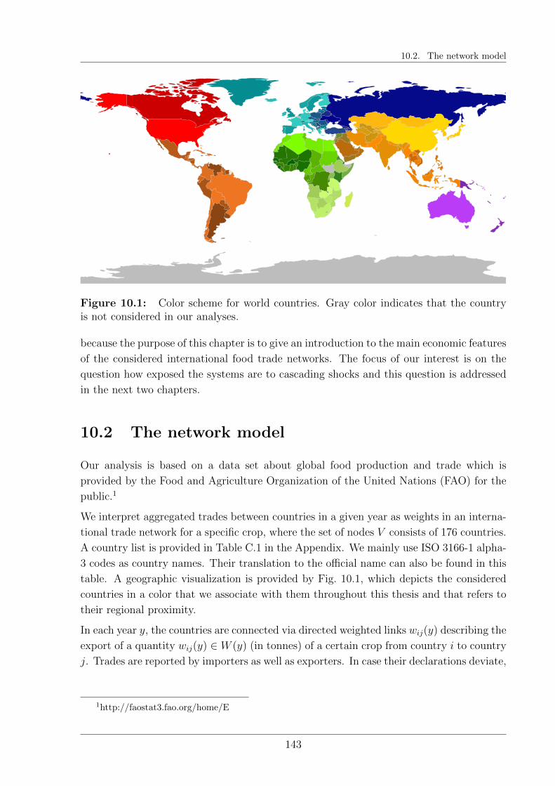
10.2. The network model
Figure 10.1: Color scheme for world countries. Gray color indicates that the countryis not considered in our analyses.
because the purpose of this chapter is to give an introduction to the main economic features
of the considered international food trade networks. The focus of our interest is on the
question how exposed the systems are to cascading shocks and this question is addressed
in the next two chapters.
10.2 The network model
Our analysis is based on a data set about global food production and trade which is
provided by the Food and Agriculture Organization of the United Nations (FAO) for the
public.1
We interpret aggregated trades between countries in a given year as weights in an interna-
tional trade network for a specific crop, where the set of nodes V consists of 176 countries.
A country list is provided in Table C.1 in the Appendix. We mainly use ISO 3166-1 alpha-
3 codes as country names. Their translation to the official name can also be found in this
table. A geographic visualization is provided by Fig. 10.1, which depicts the considered
countries in a color that we associate with them throughout this thesis and that refers to
their regional proximity.
In each year y, the countries are connected via directed weighted links wij(y) describing the
export of a quantity wij(y) ∈ W (y) (in tonnes) of a certain crop from country i to country
j. Trades are reported by importers as well as exporters. In case their declarations deviate,
1http://faostat3.fao.org/home/E
143
Chapter 10. International trade of staple food: A descriptive data analysis
we refer to the minimum of both values and thus follow a conservative estimate of the trade
interconnectivity. This way, we only consider trade between FAO reporting countries. As
our cascade models require anyway further information about production amounts and
other economic variables, e.g., their gross domestic product (GDP) or population size,
we have to restrict ourselves to a set of nodes for which this data is available. Thus, we
consider more than 85% of all international trade for maize, soy and wheat according to
the total reported FAO trades. Only for rice, we refer to ca. 65%, as a high proportion
of trade is issued between Asian countries which do not report to FAO. In future work,
the remaining variables could be partially inferred by trade reports of other countries that
trade with the missing ones. But here, we focus only on reported information.
This way, we define for each of the four staples a temporal network
G(c) =G(c)(y) = (V,W (c)(y))
2013
y=1992
that consists of 22 time slices G(c)(y), one for each year y. All of these slices consist of
the same nodes V , but vary in their weights W (c)(y). The superscript (c) indicates the
considered crop: maize (m), rice (r), soy (s), or wheat (w).
10.3 Further available information
Additional to trade volumes, we have information about financial flows along links. Con-
sequently, we can calculate the average price per quantity along a link. In this thesis, we
utilize this information only for the calculation of the average world price per quantity in
a given year. But in future, we plan to develop a model for price flows as well, since they
describe an important aspect of food security and determine who can afford food when it
becomes a scarce resource.
Alongside information about links, we consider several variables that are associated with
countries. From the trade flows, we can deduce the exports expi(y) and imports impi(y)
by each country i in a given year y.
Adding data on production quantities prodi(y), we can compute each country’s demand
as demi(y) = prodi(y) + impi(y) − expi(y). Furthermore, we have information about the
area harvested (areai(y)), the yield (yieldi(y)) and amount of produced seeds (seedi(y)).2
These can be important predictors of future production quantities or reflect expectations
of farmers.
Another important factor for future investments are prices in USD/tonne that farmers
receive at farm gate for their products prodPricei(y).3 These also depend on the usage
2http://faostat3.fao.org/download/Q/QC/E3http://faostat3.fao.org/download/P/PP/E
144
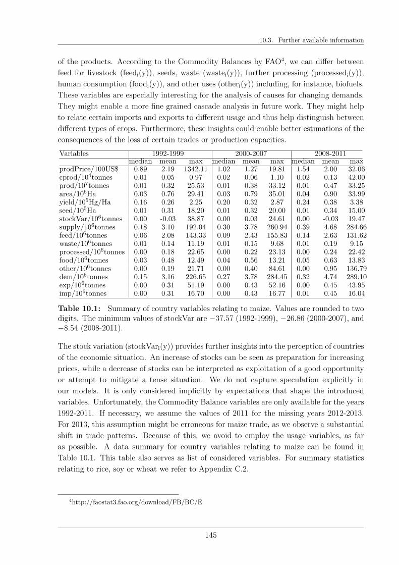
10.3. Further available information
of the products. According to the Commodity Balances by FAO4, we can differ between
feed for livestock (feedi(y)), seeds, waste (wastei(y)), further processing (processedi(y)),
human consumption (foodi(y)), and other uses (otheri(y)) including, for instance, biofuels.
These variables are especially interesting for the analysis of causes for changing demands.
They might enable a more fine grained cascade analysis in future work. They might help
to relate certain imports and exports to different usage and thus help distinguish between
different types of crops. Furthermore, these insights could enable better estimations of the
consequences of the loss of certain trades or production capacities.
Variables 1992-1999 2000-2007 2008-2011median mean max median mean max median mean max
prodPrice/100US$ 0.89 2.19 1342.11 1.02 1.27 19.81 1.54 2.00 32.06cprod/104tonnes 0.01 0.05 0.97 0.02 0.06 1.10 0.02 0.13 42.00prod/107tonnes 0.01 0.32 25.53 0.01 0.38 33.12 0.01 0.47 33.25area/106Ha 0.03 0.76 29.41 0.03 0.79 35.01 0.04 0.90 33.99yield/105Hg/Ha 0.16 0.26 2.25 0.20 0.32 2.87 0.24 0.38 3.38seed/105Ha 0.01 0.31 18.20 0.01 0.32 20.00 0.01 0.34 15.00stockVar/106tonnes 0.00 -0.03 38.87 0.00 0.03 24.61 0.00 -0.03 19.47supply/106tonnes 0.18 3.10 192.04 0.30 3.78 260.94 0.39 4.68 284.66feed/106tonnes 0.06 2.08 143.33 0.09 2.43 155.83 0.14 2.63 131.62waste/106tonnes 0.01 0.14 11.19 0.01 0.15 9.68 0.01 0.19 9.15processed/106tonnes 0.00 0.18 22.65 0.00 0.22 23.13 0.00 0.24 22.42food/106tonnes 0.03 0.48 12.49 0.04 0.56 13.21 0.05 0.63 13.83other/106tonnes 0.00 0.19 21.71 0.00 0.40 84.61 0.00 0.95 136.79dem/106tonnes 0.15 3.16 226.65 0.27 3.78 284.45 0.32 4.74 289.10exp/106tonnes 0.00 0.31 51.19 0.00 0.43 52.16 0.00 0.45 43.95imp/106tonnes 0.00 0.31 16.70 0.00 0.43 16.77 0.01 0.45 16.04
Table 10.1: Summary of country variables relating to maize. Values are rounded to twodigits. The minimum values of stockVar are −37.57 (1992-1999), −26.86 (2000-2007), and−8.54 (2008-2011).
The stock variation (stockVari(y)) provides further insights into the perception of countries
of the economic situation. An increase of stocks can be seen as preparation for increasing
prices, while a decrease of stocks can be interpreted as exploitation of a good opportunity
or attempt to mitigate a tense situation. We do not capture speculation explicitly in
our models. It is only considered implicitly by expectations that shape the introduced
variables. Unfortunately, the Commodity Balance variables are only available for the years
1992-2011. If necessary, we assume the values of 2011 for the missing years 2012-2013.
For 2013, this assumption might be erroneous for maize trade, as we observe a substantial
shift in trade patterns. Because of this, we avoid to employ the usage variables, as far
as possible. A data summary for country variables relating to maize can be found in
Table 10.1. This table also serves as list of considered variables. For summary statistics
relating to rice, soy or wheat we refer to Appendix C.2.
4http://faostat3.fao.org/download/FB/BC/E
145
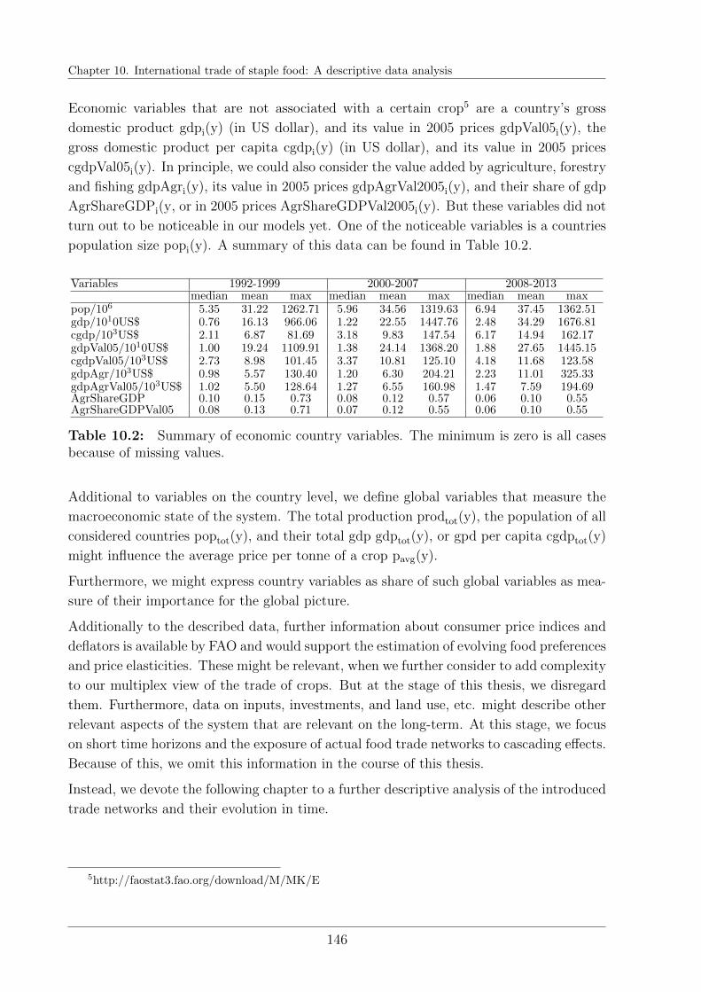
Chapter 10. International trade of staple food: A descriptive data analysis
Economic variables that are not associated with a certain crop5 are a country’s gross
domestic product gdpi(y) (in US dollar), and its value in 2005 prices gdpVal05i(y), the
gross domestic product per capita cgdpi(y) (in US dollar), and its value in 2005 prices
cgdpVal05i(y). In principle, we could also consider the value added by agriculture, forestry
and fishing gdpAgri(y), its value in 2005 prices gdpAgrVal2005i(y), and their share of gdp
AgrShareGDPi(y, or in 2005 prices AgrShareGDPVal2005i(y). But these variables did not
turn out to be noticeable in our models yet. One of the noticeable variables is a countries
population size popi(y). A summary of this data can be found in Table 10.2.
Variables 1992-1999 2000-2007 2008-2013median mean max median mean max median mean max
pop/106 5.35 31.22 1262.71 5.96 34.56 1319.63 6.94 37.45 1362.51gdp/1010US$ 0.76 16.13 966.06 1.22 22.55 1447.76 2.48 34.29 1676.81cgdp/103US$ 2.11 6.87 81.69 3.18 9.83 147.54 6.17 14.94 162.17gdpVal05/1010US$ 1.00 19.24 1109.91 1.38 24.14 1368.20 1.88 27.65 1445.15cgdpVal05/103US$ 2.73 8.98 101.45 3.37 10.81 125.10 4.18 11.68 123.58gdpAgr/103US$ 0.98 5.57 130.40 1.20 6.30 204.21 2.23 11.01 325.33gdpAgrVal05/103US$ 1.02 5.50 128.64 1.27 6.55 160.98 1.47 7.59 194.69AgrShareGDP 0.10 0.15 0.73 0.08 0.12 0.57 0.06 0.10 0.55AgrShareGDPVal05 0.08 0.13 0.71 0.07 0.12 0.55 0.06 0.10 0.55
Table 10.2: Summary of economic country variables. The minimum is zero is all casesbecause of missing values.
Additional to variables on the country level, we define global variables that measure the
macroeconomic state of the system. The total production prodtot(y), the population of all
considered countries poptot(y), and their total gdp gdptot(y), or gpd per capita cgdptot(y)
might influence the average price per tonne of a crop pavg(y).
Furthermore, we might express country variables as share of such global variables as mea-
sure of their importance for the global picture.
Additionally to the described data, further information about consumer price indices and
deflators is available by FAO and would support the estimation of evolving food preferences
and price elasticities. These might be relevant, when we further consider to add complexity
to our multiplex view of the trade of crops. But at the stage of this thesis, we disregard
them. Furthermore, data on inputs, investments, and land use, etc. might describe other
relevant aspects of the system that are relevant on the long-term. At this stage, we focus
on short time horizons and the exposure of actual food trade networks to cascading effects.
Because of this, we omit this information in the course of this thesis.
Instead, we devote the following chapter to a further descriptive analysis of the introduced
trade networks and their evolution in time.
5http://faostat3.fao.org/download/M/MK/E
146
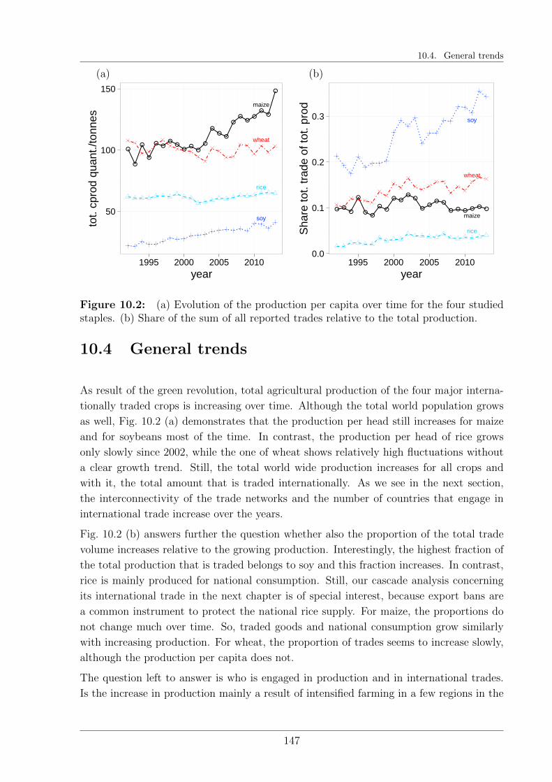
10.4. General trends
maize
rice
soy
wheat
50
100
150
1995 2000 2005 2010year
tot.
cpro
d qu
ant./
tonn
es
maize
rice
soy
wheat
0.0
0.1
0.2
0.3
1995 2000 2005 2010year
Sha
re to
t. tr
ade
of to
t. pr
od
(a) (b)
Figure 10.2: (a) Evolution of the production per capita over time for the four studiedstaples. (b) Share of the sum of all reported trades relative to the total production.
10.4 General trends
As result of the green revolution, total agricultural production of the four major interna-
tionally traded crops is increasing over time. Although the total world population grows
as well, Fig. 10.2 (a) demonstrates that the production per head still increases for maize
and for soybeans most of the time. In contrast, the production per head of rice grows
only slowly since 2002, while the one of wheat shows relatively high fluctuations without
a clear growth trend. Still, the total world wide production increases for all crops and
with it, the total amount that is traded internationally. As we see in the next section,
the interconnectivity of the trade networks and the number of countries that engage in
international trade increase over the years.
Fig. 10.2 (b) answers further the question whether also the proportion of the total trade
volume increases relative to the growing production. Interestingly, the highest fraction of
the total production that is traded belongs to soy and this fraction increases. In contrast,
rice is mainly produced for national consumption. Still, our cascade analysis concerning
its international trade in the next chapter is of special interest, because export bans are
a common instrument to protect the national rice supply. For maize, the proportions do
not change much over time. So, traded goods and national consumption grow similarly
with increasing production. For wheat, the proportion of trades seems to increase slowly,
although the production per capita does not.
The question left to answer is who is engaged in production and in international trades.
Is the increase in production mainly a result of intensified farming in a few regions in the
147
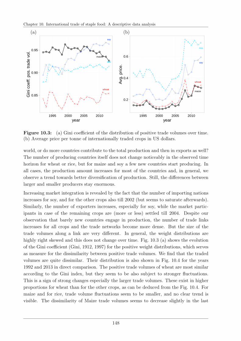
Chapter 10. International trade of staple food: A descriptive data analysis
maize
rice
soy
wheat
0.85
0.90
0.95
1995 2000 2005 2010year
Gin
i coe
ff. p
os. t
rade
vol
.
maize
rice
soy
wheat
0.2
0.4
0.6
1995 2000 2005 2010year
Avg
. pric
e.
(a) (b)
Figure 10.3: (a) Gini coefficient of the distribution of positive trade volumes over time.(b) Average price per tonne of internationally traded crops in US dollars.
world, or do more countries contribute to the total production and then in exports as well?
The number of producing countries itself does not change noticeably in the observed time
horizon for wheat or rice, but for maize and soy a few new countries start producing. In
all cases, the production amount increases for most of the countries and, in general, we
observe a trend towards better diversification of production. Still, the differences between
larger and smaller producers stay enormous.
Increasing market integration is revealed by the fact that the number of importing nations
increases for soy, and for the other crops also till 2002 (but seems to saturate afterwards).
Similarly, the number of exporters increases, especially for soy, while the market partic-
ipants in case of the remaining crops are (more or less) settled till 2004. Despite our
observation that barely new countries engage in production, the number of trade links
increases for all crops and the trade networks become more dense. But the size of the
trade volumes along a link are very different. In general, the weight distributions are
highly right skewed and this does not change over time. Fig. 10.3 (a) shows the evolution
of the Gini coefficient (Gini, 1912, 1997) for the positive weight distributions, which serves
as measure for the dissimilarity between positive trade volumes. We find that the traded
volumes are quite dissimilar. Their distribution is also shown in Fig. 10.4 for the years
1992 and 2013 in direct comparison. The positive trade volumes of wheat are most similar
according to the Gini index, but they seem to be also subject to stronger fluctuations.
This is a sign of strong changes especially the larger trade volumes. These exist in higher
proportions for wheat than for the other crops, as can be deduced from the Fig. 10.4. For
maize and for rice, trade volume fluctuations seem to be smaller, and no clear trend is
visible. The dissimilarity of Maize trade volumes seems to decrease slightly in the last
148
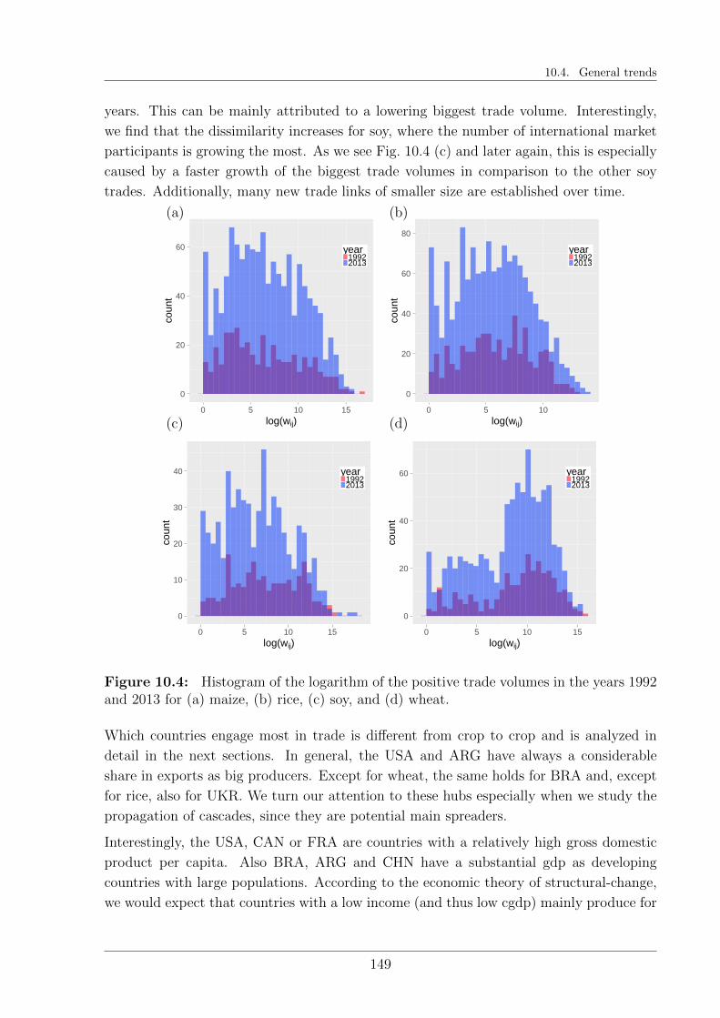
10.4. General trends
years. This can be mainly attributed to a lowering biggest trade volume. Interestingly,
we find that the dissimilarity increases for soy, where the number of international market
participants is growing the most. As we see Fig. 10.4 (c) and later again, this is especially
caused by a faster growth of the biggest trade volumes in comparison to the other soy
trades. Additionally, many new trade links of smaller size are established over time.
0
20
40
60
0 5 10 15log(wij)
coun
t
year19922013
0
20
40
60
80
0 5 10log(wij)
coun
t
year19922013
0
10
20
30
40
0 5 10 15log(wij)
coun
t
year19922013
0
20
40
60
0 5 10 15log(wij)
coun
t
year19922013
(a) (b)
(c) (d)
Figure 10.4: Histogram of the logarithm of the positive trade volumes in the years 1992and 2013 for (a) maize, (b) rice, (c) soy, and (d) wheat.
Which countries engage most in trade is different from crop to crop and is analyzed in
detail in the next sections. In general, the USA and ARG have always a considerable
share in exports as big producers. Except for wheat, the same holds for BRA and, except
for rice, also for UKR. We turn our attention to these hubs especially when we study the
propagation of cascades, since they are potential main spreaders.
Interestingly, the USA, CAN or FRA are countries with a relatively high gross domestic
product per capita. Also BRA, ARG and CHN have a substantial gdp as developing
countries with large populations. According to the economic theory of structural-change,
we would expect that countries with a low income (and thus low cgdp) mainly produce for
149
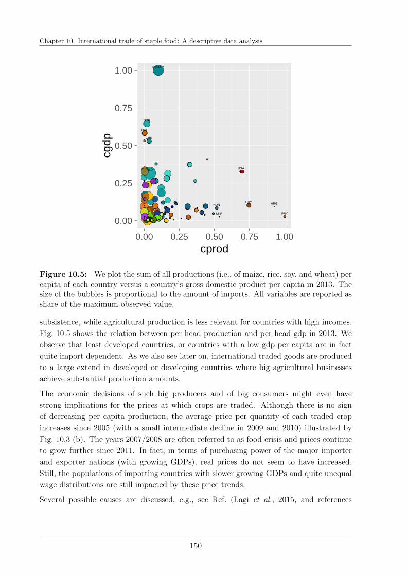
Chapter 10. International trade of staple food: A descriptive data analysis
USA
ARG
PRY
URY
NLD
NOR
CHE
BELLUX
HUN
UKRTWN
QAT
0.00
0.25
0.50
0.75
1.00
0.00 0.25 0.50 0.75 1.00cprod
cgdp
Figure 10.5: We plot the sum of all productions (i.e., of maize, rice, soy, and wheat) percapita of each country versus a country’s gross domestic product per capita in 2013. Thesize of the bubbles is proportional to the amount of imports. All variables are reported asshare of the maximum observed value.
subsistence, while agricultural production is less relevant for countries with high incomes.
Fig. 10.5 shows the relation between per head production and per head gdp in 2013. We
observe that least developed countries, or countries with a low gdp per capita are in fact
quite import dependent. As we also see later on, international traded goods are produced
to a large extend in developed or developing countries where big agricultural businesses
achieve substantial production amounts.
The economic decisions of such big producers and of big consumers might even have
strong implications for the prices at which crops are traded. Although there is no sign
of decreasing per capita production, the average price per quantity of each traded crop
increases since 2005 (with a small intermediate decline in 2009 and 2010) illustrated by
Fig. 10.3 (b). The years 2007/2008 are often referred to as food crisis and prices continue
to grow further since 2011. In fact, in terms of purchasing power of the major importer
and exporter nations (with growing GDPs), real prices do not seem to have increased.
Still, the populations of importing countries with slower growing GDPs and quite unequal
wage distributions are still impacted by these price trends.
Several possible causes are discussed, e.g., see Ref. (Lagi et al., 2015, and references
150

10.5. International trade of maize
therein). As main factors, an increased demand for bio fuels (mainly obtained from maize
or soy), price speculation, an increasing demand for meat in developing countries, whose
production requires a higher amount of feed, and bad weather are investigated. All of the
different causes affect either the production or demand side. Our cascade models serve
the purpose to study the implications of such factors on the trade network topology.
We note high correlations between the price evolution of the different crops. This is not
surprising, as the staples can substitute each other partially. As explained in the intro-
duction of Part III, when one crop becomes more expensive the preferences of consumers
might shift towards a cheaper crop. Thus, the demand for the latter increases, which leads
to a price increase of the at first cheaper crop. The coupling of the prices suggests that a
cascade model for food trade should consider a multiplex perspective, where the different
networks are coupled by prices, for instance.
Before we discuss further details of a good cascade model, we focus on directly observed
trade relationships between countries in the next sections.
10.5 International trade of maize
As the nodes in our trade networks refer to countries, they incorporate geographic in-
formation. Usually we do not illustrate networks on maps, because the high number of
trade links challenges the identification of trade partners. Nevertheless, we encode regional
information by similar colors that we associate with countries and that are depicted in
Fig. 10.1. A trade link is then associated with the color of the exporter nation. Fig. 10.6
displays four snapshots of the temporal network of maize trades in 1992, 2000, 2008, and
2013.
As mentioned earlier, we observe a clear increase in the number of economic actors and in
coupling strength of the network. In 1992, the USA dominated the international market.
Considering that it produces almost 46% of the world wide maize production, this is not
astonishing. ARG, CAN and AUS are additional bigger exporters that serve other conti-
nents, while CHN mainly serves the Asian market, and FRA and HUN export primarily
within Europe. Over the years, further countries cultivate maize so that the share of the
production by the USA declines to 35% in 2013. Accordingly, additional exporters and
importers enter the market.
Fig. 10.7 displays the production of 20 largest producers relative to total production in
2000 and 2012. Additionally, a darker color indicates how much of this production covers
their demand. The USA clearly is the top producer (and stays the biggest exporter till
2012). Also the production of CHN grows noticeably till 2012 but its demand increases
even faster so that CHN becomes a net importer. In fact, a number of main producers
have a higher demand than they can serve by their own production: Besides CHN, also
151
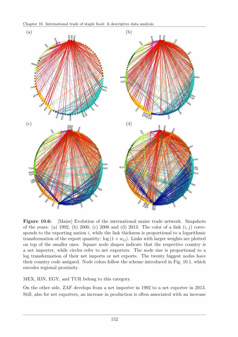
Chapter 10. International trade of staple food: A descriptive data analysis
US
AC
AN
AR
G
FRADEU
NLD
PRT
CH
E
GB
R
HU
N
PO
L
SV
NCH
NJPN
TWN
MYS
THA
MAR
ZAF
AUS
US
A
AR
G
CO
L
NIC
FRA
PRTESPGBR
HU
N
PO
LRU
SC
HN
HK
GJP
NKO
R
LKA
DZA
MAR
ZAF
AU
S
US
AC
AN
AR
G
BR
A
FRA
GRC
GBR
CYPHUN
PO
L
UK
RJPN
IND
MYS
JORLBN
DZAMAR
TUN
ZAF
US
A
AR
G
BR
A
PRY
FRA
IRLITA
NLD
GBR
BGR
HUN
RO
U
RU
SU
KR
JPN
KOR
TWNIN
D
EGY
ZAF
(a) (b)
(c) (d)
Figure 10.6: [Maize] Evolution of the international maize trade network. Snapshotsof the years: (a) 1992, (b) 2000, (c) 2008 and (d) 2013. The color of a link (i, j) corre-sponds to the exporting nation i, while the link thickness is proportional to a logarithmictransformation of the export quantity: log (1 + wij). Links with larger weights are plottedon top of the smaller ones. Square node shapes indicate that the respective country isa net importer, while circles refer to net exporters. The node size is proportional to alog transformation of their net imports or net exports. The twenty biggest nodes havetheir country code assigned. Node colors follow the scheme introduced in Fig. 10.1, whichencodes regional proximity.
MEX, IDN, EGY, and TUR belong to this category.
On the other side, ZAF develops from a net importer in 1992 to a net exporter in 2013.
Still, also for net exporters, an increase in production is often associated with an increase
152
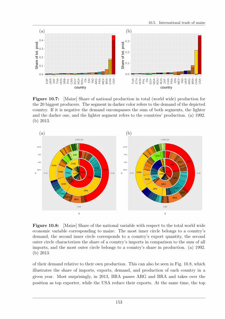
10.5. International trade of maize
0.0
0.1
0.2
0.3
0.4
ES
PU
KR
ZA
FT
HA
HU
NS
RB
PH
LC
AN
EG
YN
GA
RO
UIT
AID
NIN
DA
RG
FR
AM
EX
BR
AC
HN
US
A
country
Sha
re o
f tot
. pro
d.
0.0
0.1
0.2
0.3
TU
RE
TH
HU
NP
HL
ITA
EG
YN
GA
RO
UR
US
ZA
FC
AN
FR
AID
NM
EX
IND
UK
RA
RG
BR
AC
HN
US
A
country
Sha
re o
f tot
. pro
d.
(a) (b)
Figure 10.7: [Maize] Share of national production in total (world wide) production forthe 20 biggest producers. The segment in darker color refers to the demand of the depictedcountry. If it is negative the demand encompasses the sum of both segments, the lighterand the darker one, and the lighter segment refers to the countries’ production. (a) 1992.(b) 2013.
USA
CHN
BRAMEX
FRA
USACHN
JPN
KOR
TWN
ZAF
ESP
USA
CHN
FRA
ARGCAN
0.25
0.50
0.75
0.00/1.00
dem
exp
imp
prod
y
x
USA
CHN
BRA
ARGUKR
USACHN
JPN
KOR
MEX
ESP
EGY
BRA
USA
ARG
UKR
FRA
0.25
0.50
0.75
0.00/1.00
dem
exp
imp
prod
y
x
(a) (b)
Figure 10.8: [Maize] Share of the national variable with respect to the total world wideeconomic variable corresponding to maize. The most inner circle belongs to a country’sdemand, the second inner circle corresponds to a country’s export quantity, the secondouter circle characterizes the share of a country’s imports in comparison to the sum of allimports, and the most outer circle belongs to a country’s share in production. (a) 1992.(b) 2013.
of their demand relative to their own production. This can also be seen in Fig. 10.8, which
illustrates the share of imports, exports, demand, and production of each country in a
given year. Most surprisingly, in 2013, BRA passes ARG and BRA and takes over the
position as top exporter, while the USA reduce their exports. At the same time, the top
153
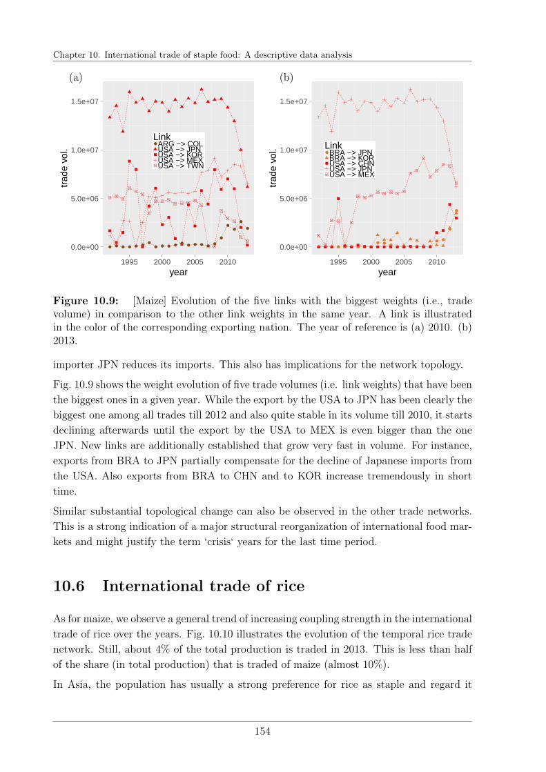
Chapter 10. International trade of staple food: A descriptive data analysis
0.0e+00
5.0e+06
1.0e+07
1.5e+07
1995 2000 2005 2010year
trad
e vo
l.
Link ARG −> COLUSA −> JPNUSA −> KORUSA −> MEXUSA −> TWN
0.0e+00
5.0e+06
1.0e+07
1.5e+07
1995 2000 2005 2010year
trad
e vo
l. Link BRA −> JPNBRA −> KORUSA −> CHNUSA −> JPNUSA −> MEX
(a) (b)
Figure 10.9: [Maize] Evolution of the five links with the biggest weights (i.e., tradevolume) in comparison to the other link weights in the same year. A link is illustratedin the color of the corresponding exporting nation. The year of reference is (a) 2010. (b)2013.
importer JPN reduces its imports. This also has implications for the network topology.
Fig. 10.9 shows the weight evolution of five trade volumes (i.e. link weights) that have been
the biggest ones in a given year. While the export by the USA to JPN has been clearly the
biggest one among all trades till 2012 and also quite stable in its volume till 2010, it starts
declining afterwards until the export by the USA to MEX is even bigger than the one
JPN. New links are additionally established that grow very fast in volume. For instance,
exports from BRA to JPN partially compensate for the decline of Japanese imports from
the USA. Also exports from BRA to CHN and to KOR increase tremendously in short
time.
Similar substantial topological change can also be observed in the other trade networks.
This is a strong indication of a major structural reorganization of international food mar-
kets and might justify the term ‘crisis‘ years for the last time period.
10.6 International trade of rice
As for maize, we observe a general trend of increasing coupling strength in the international
trade of rice over the years. Fig. 10.10 illustrates the evolution of the temporal rice trade
network. Still, about 4% of the total production is traded in 2013. This is less than half
of the share (in total production) that is traded of maize (almost 10%).
In Asia, the population has usually a strong preference for rice as staple and regard it
154

10.6. International trade of rice
US
AC
AN
PER
URY
AUT
IRLITA
NOR
ESPSWE
CH
E
PO
LR
OUCH
N
INDPAK
THA
KWT
EGY
SEN
US
AC
AN
GUY
URY
FIN
ITA
NORESPSWECHE
TU
R
RU
SC
HN
INDPA
K
THASAU
LBNISREGY
US
AC
AN
AR
G
BR
A
GUY
URY
GRC
IRLITA
NORESPSWECHE
RO
U
CH
N
INDPA
K
THA
SYR
SEN
US
AC
AN
AR
G
BR
A
GUY
URY
FIN
GRC
ITA
NORESPSWECHE
ALB
INDPA
KKHM
THA
EGY
AU
S
(a) (b)
(c) (d)
Figure 10.10: [Rice] Evolution of the international rice trade network. Snapshots of theyears: (a) 1992, (b) 2000, (c) 2008 and (d) 2013. The color of a link (i, j) corresponds to theexporting nation i, while the link thickness is proportional to a logarithmic transformationof the export quantity: log (1 + wij). Links with larger weights are plotted on top of thesmaller ones. Square node shapes indicate that the respective country is a net importer,while circles refer to net exporters. The node size is proportional to a log transformationof their net imports or net exports.
as important for their culture. Consequently, national production is sometimes subject
to export (or even import) restrictions or other protective policies. Rice is often first
produced for national consumption, while overproduction is traded.
Consequently, the biggest five producers are Asian countries. Fig. 10.11 depicts the share
of the 20 biggest producers in production and their demands. CHN leads clearly with
155
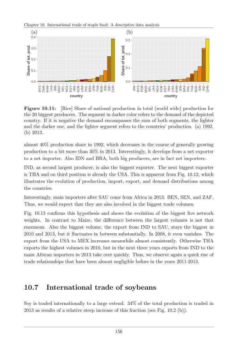
Chapter 10. International trade of staple food: A descriptive data analysis
0.0
0.1
0.2
0.3
0.4M
YS
TW
NK
HM
LKA
IRN
MD
GN
PL
NG
AE
GY
PAK
KO
RU
SA
PH
LB
RA
JPN
TH
AB
GD
IDN
IND
CH
N
country
Sha
re o
f tot
. pro
d.
0.0
0.1
0.2
0.3
IRN
MY
SP
ER
MD
GN
PL
LKA
NG
AK
OR
EG
YPA
KU
SA
KH
MJP
NB
RA
PH
LT
HA
BG
DID
NIN
DC
HN
country
Sha
re o
f tot
. pro
d.
(a) (b)
Figure 10.11: [Rice] Share of national production in total (world wide) production forthe 20 biggest producers. The segment in darker color refers to the demand of the depictedcountry. If it is negative the demand encompasses the sum of both segments, the lighterand the darker one, and the lighter segment refers to the countries’ production. (a) 1992.(b) 2013.
almost 40% production share in 1992, which decreases in the course of generally growing
production to a bit more than 30% in 2013. Interestingly, it develops from a net exporter
to a net importer. Also IDN and BRA, both big producers, are in fact net importers.
IND, as second largest producer, is also the biggest exporter. The next biggest exporter
is THA and on third position is already the USA. This is apparent from Fig. 10.12, which
illustrates the evolution of production, import, export, and demand distributions among
the countries.
Interestingly, main importers after SAU come from Africa in 2013: BEN, SEN, and ZAF.
Thus, we would expect that they are also involved in the biggest trade volumes.
Fig. 10.13 confirms this hypothesis and shows the evolution of the biggest five network
weights. In contrast to Maize, the difference between the largest volumes is not that
enormous. Also the biggest volume, the export from IND to SAU, stays the biggest in
2010 and 2013, but it fluctuates in between substantially. In 2008, it even vanishes. The
export from the USA to MEX increases meanwhile almost consistently. Otherwise THA
exports the highest volumes in 2010, but in the next three years exports from IND to the
main African importers in 2013 take over quickly. Thus, we observe again a quick rise of
trade relationships that have been almost negligible before in the years 2011-2013.
10.7 International trade of soybeans
Soy is traded internationally to a large extend. 34% of the total production is traded in
2013 as results of a relative steep increase of this fraction (see Fig. 10.2 (b)).
156
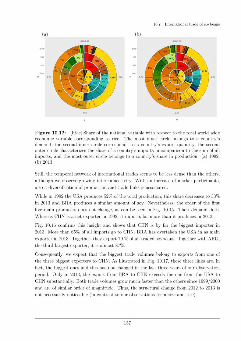
10.7. International trade of soybeans
CHN
IND
IDN
BGD
THA
CHNIND
IDN
BRA
HKG
ZAF
FRATHA
USA
ITA
URY
PAK
0.25
0.50
0.75
0.00/1.00
dem
exp
imp
prod
y
x
CHN
IND
IDN
BGD
THA
CHN
IND
SAU
BEN
SEN
ZAF BRA
IND
THAUSA
PAKITA 0.25
0.50
0.75
0.00/1.00
dem
exp
imp
prod
y
x
(a) (b)
Figure 10.12: [Rice] Share of the national variable with respect to the total world wideeconomic variable corresponding to rice. The most inner circle belongs to a country’sdemand, the second inner circle corresponds to a country’s export quantity, the secondouter circle characterizes the share of a country’s imports in comparison to the sum of allimports, and the most outer circle belongs to a country’s share in production. (a) 1992.(b) 2013.
Still, the temporal network of international trades seems to be less dense than the others,
although we observe growing interconnectivity. With an increase of market participants,
also a diversification of production and trade links is associated.
While in 1992 the USA produces 52% of the total production, this share decreases to 33%
in 2013 and BRA produces a similar amount of soy. Nevertheless, the order of the first
five main producers does not change, as can be seen in Fig. 10.15. Their demand does.
Whereas CHN is a net exporter in 1992, it imports far more than it produces in 2013.
Fig. 10.16 confirms this insight and shows that CHN is by far the biggest importer in
2013. More than 65% of all imports go to CHN. BRA has overtaken the USA in as main
exporter in 2013. Together, they export 79 % of all traded soybeans. Together with ARG,
the third largest exporter, it is almost 87%.
Consequently, we expect that the biggest trade volumes belong to exports from one of
the three biggest exporters to CHN. As illustrated in Fig. 10.17, these three links are, in
fact, the biggest ones and this has not changed in the last three years of our observation
period. Only in 2013, the export from BRA to CHN exceeds the one from the USA to
CHN substantially. Both trade volumes grow much faster than the others since 1999/2000
and are of similar order of magnitude. Thus, the structural change from 2012 to 2013 is
not necessarily noticeable (in contrast to our observations for maize and rice).
157
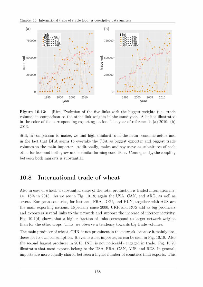
Chapter 10. International trade of staple food: A descriptive data analysis
0
250000
500000
750000
1995 2000 2005 2010year
trad
e vo
l.
Link IND −> SAUTHA −> CIVTHA −> PHLTHA −> ZAFUSA −> MEX
0
250000
500000
750000
1995 2000 2005 2010year
trad
e vo
l.
Link IND −> BENIND −> SAUIND −> SENIND −> ZAFUSA −> MEX
(a) (b)
Figure 10.13: [Rice] Evolution of the five links with the biggest weights (i.e., tradevolume) in comparison to the other link weights in the same year. A link is illustratedin the color of the corresponding exporting nation. The year of reference is (a) 2010. (b)2013.
Still, in comparison to maize, we find high similarities in the main economic actors and
in the fact that BRA seems to overtake the USA as biggest exporter and biggest trade
volumes to the main importer. Additionally, maize and soy serve as substitutes of each
other for feed and both grow under similar farming conditions. Consequently, the coupling
between both markets is substantial.
10.8 International trade of wheat
Also in case of wheat, a substantial share of the total production is traded internationally,
i.e. 16% in 2013. As we see in Fig. 10.18, again the USA, CAN, and ARG, as well as
several European countries, for instance, FRA, DEU, and HUN, together with AUS are
the main exporting nations. Especially since 2000, UKR and RUS add as big producers
and exporters several links to the network and support the increase of interconnectivity.
Fig. 10.4(d) shows that a higher fraction of links correspond to larger network weights
than for the other crops. Thus, we observe a tendency towards big trade volumes.
The main producer of wheat, CHN, is not prominent in the network, because it mainly pro-
duces for its own consumption. It even is a net importer, as can be seen in Fig. 10.19. Also
the second largest producer in 2013, IND, is not noticeably engaged in trade. Fig. 10.20
illustrates that most exports belong to the USA, FRA, CAN, AUS, and RUS. In general,
imports are more equally shared between a higher number of countries than exports. This
158

10.8. International trade of wheat
US
A
CA
NA
RG
BR
A
PRY
FRA
GRC
ITANO
R
PR
T
ES
P
CH
E
BE
LLU
X
CHN
JPN
TWN
IDN
MYS
PHL
SGP
US
AC
AN
AR
G
BR
A
CO
L
PRY
FRA
IRLITA
ESPCH
E
BE
LLUX
TUR
JPNKOR
TWN
IDN
PHL
THA
AU
S
US
AC
AN
AR
G
BR
A
PRY
PER
AUTDNK
DEU
PRTESP
GBR
TU
RUK
R
CH
NJPNKO
R
INDIDN
PHL
US
AC
AN
AR
G
BO
LB
RA
PRY
URY
ITA
PRTESP
UK
RC
HNJP
NKORTW
N
IND
IDNMYS
THA
EGY
(a) (b)
(c) (d)
Figure 10.14: [Soy] Evolution of the international soybean trade network. Snapshotsof the years: (a) 1992, (b) 2000, (c) 2008 and (d) 2013. The color of a link (i, j) corre-sponds to the exporting nation i, while the link thickness is proportional to a logarithmictransformation of the export quantity: log (1 + wij). Links with larger weights are plottedon top of the smaller ones. Square node shapes indicate that the respective country isa net importer, while circles refer to net exporters. The node size is proportional to alog transformation of their net imports or net exports. The twenty biggest nodes havetheir country code assigned. Node colors follow the scheme introduced in Fig. 10.1, whichencodes regional proximity.
tendency becomes stronger, as especially CHN and JPN reduce their share in total imports
over the years. Still, they stay among the biggest importers after to BRA, IDN, and DZA.
Interestingly, the largest trade volume in 2010 belongs to the export of wheat from ARG
159
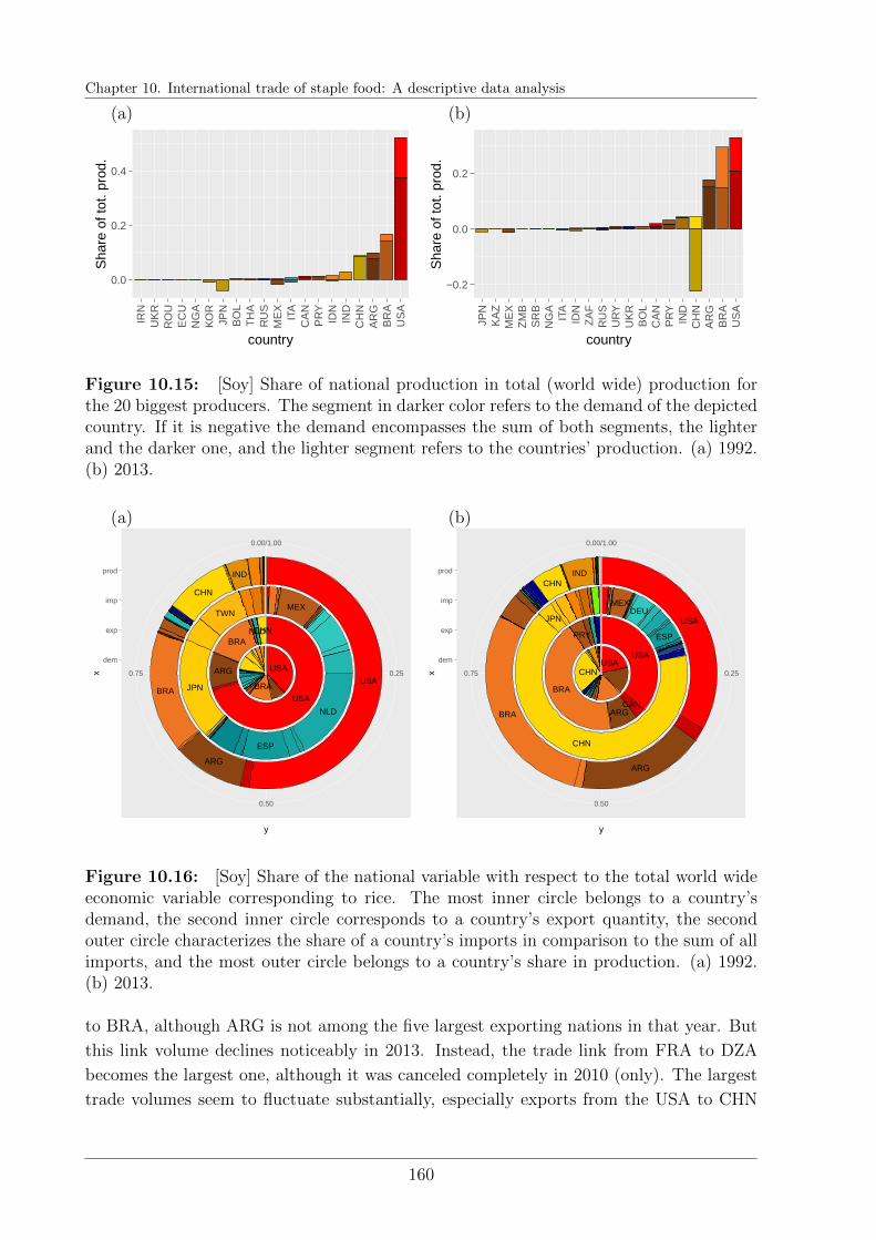
Chapter 10. International trade of staple food: A descriptive data analysis
0.0
0.2
0.4
IRN
UK
RR
OU
EC
UN
GA
KO
RJP
NB
OL
TH
AR
US
ME
XIT
AC
AN
PR
YID
NIN
DC
HN
AR
GB
RA
US
A
country
Sha
re o
f tot
. pro
d.
−0.2
0.0
0.2
JPN
KA
ZM
EX
ZM
BS
RB
NG
AIT
AID
NZ
AF
RU
SU
RY
UK
RB
OL
CA
NP
RY
IND
CH
NA
RG
BR
AU
SA
country
Sha
re o
f tot
. pro
d.
(a) (b)
Figure 10.15: [Soy] Share of national production in total (world wide) production forthe 20 biggest producers. The segment in darker color refers to the demand of the depictedcountry. If it is negative the demand encompasses the sum of both segments, the lighterand the darker one, and the lighter segment refers to the countries’ production. (a) 1992.(b) 2013.
USABRA
ARG
CHN
IND
USA
BRAJPN
NLD
TWN
ESP
MEX
USA
BRA
ARG
CHNNLD
0.25
0.50
0.75
0.00/1.00
dem
exp
imp
prod
y
x
USA
BRA
ARG
CHNIND
CHNUSA
CHN
MEX
ESP
DEUJPN
BRA
USA
ARG
PRY
CAN
0.25
0.50
0.75
0.00/1.00
dem
exp
imp
prod
y
x
(a) (b)
Figure 10.16: [Soy] Share of the national variable with respect to the total world wideeconomic variable corresponding to rice. The most inner circle belongs to a country’sdemand, the second inner circle corresponds to a country’s export quantity, the secondouter circle characterizes the share of a country’s imports in comparison to the sum of allimports, and the most outer circle belongs to a country’s share in production. (a) 1992.(b) 2013.
to BRA, although ARG is not among the five largest exporting nations in that year. But
this link volume declines noticeably in 2013. Instead, the trade link from FRA to DZA
becomes the largest one, although it was canceled completely in 2010 (only). The largest
trade volumes seem to fluctuate substantially, especially exports from the USA to CHN
160
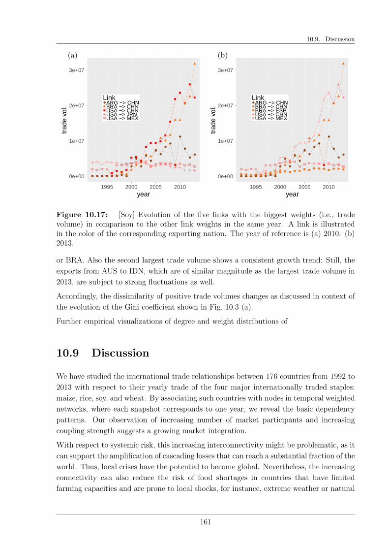
10.9. Discussion
0e+00
1e+07
2e+07
3e+07
1995 2000 2005 2010year
trad
e vo
l.
Link ARG −> CHNBRA −> CHNUSA −> CHNUSA −> JPNUSA −> MEX
0e+00
1e+07
2e+07
3e+07
1995 2000 2005 2010year
trad
e vo
l.
Link ARG −> CHNBRA −> CHNBRA −> ESPUSA −> CHNUSA −> MEX
(a) (b)
Figure 10.17: [Soy] Evolution of the five links with the biggest weights (i.e., tradevolume) in comparison to the other link weights in the same year. A link is illustratedin the color of the corresponding exporting nation. The year of reference is (a) 2010. (b)2013.
or BRA. Also the second largest trade volume shows a consistent growth trend: Still, the
exports from AUS to IDN, which are of similar magnitude as the largest trade volume in
2013, are subject to strong fluctuations as well.
Accordingly, the dissimilarity of positive trade volumes changes as discussed in context of
the evolution of the Gini coefficient shown in Fig. 10.3 (a).
Further empirical visualizations of degree and weight distributions of
10.9 Discussion
We have studied the international trade relationships between 176 countries from 1992 to
2013 with respect to their yearly trade of the four major internationally traded staples:
maize, rice, soy, and wheat. By associating such countries with nodes in temporal weighted
networks, where each snapshot corresponds to one year, we reveal the basic dependency
patterns. Our observation of increasing number of market participants and increasing
coupling strength suggests a growing market integration.
With respect to systemic risk, this increasing interconnectivity might be problematic, as it
can support the amplification of cascading losses that can reach a substantial fraction of the
world. Thus, local crises have the potential to become global. Nevertheless, the increasing
connectivity can also reduce the risk of food shortages in countries that have limited
farming capacities and are prone to local shocks, for instance, extreme weather or natural
161
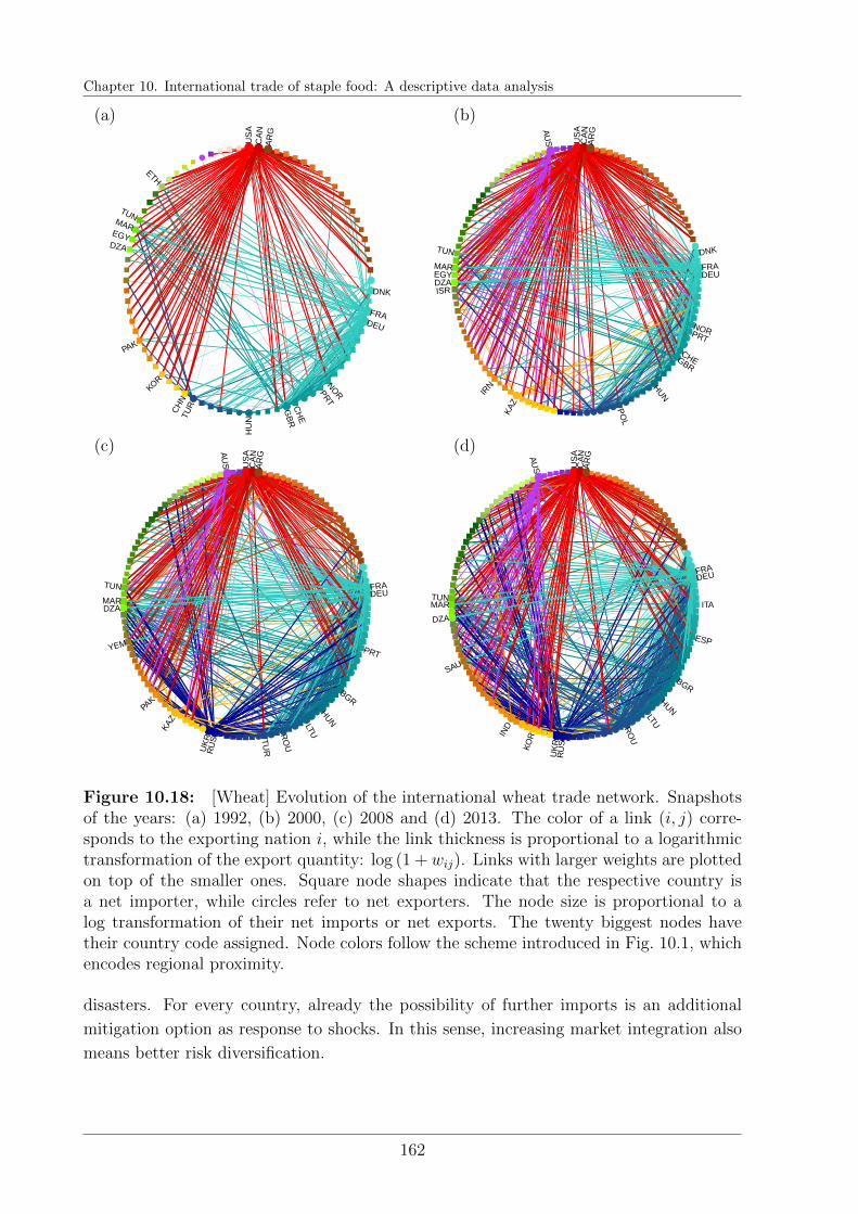
Chapter 10. International trade of staple food: A descriptive data analysis
US
AC
AN
AR
G
DNK
FRADEU
NORPRT
CH
E
GB
R
HU
NTURCH
N
KOR
PAK
DZA
EGY
MAR
TUN
ETH
US
AC
AN
AR
G
DNK
FRADEU
NORPRT
CHEGBR
HUN
PO
L
KA
Z
IRN
ISRDZAEGYMAR
TUN
AU
S
US
AC
AN
AR
G
FRADEU
PRT
BGR
HUNLTURO
U
TU
RRU
SU
KR
KAZ
PAK
YEM
DZAMAR
TUN
AU
S
US
AC
AN
AR
G
FRADEU
ITA
ESP
BGR
HUN
LTURO
U
RU
SU
KR
KO
RIND
SAU
DZA
MARTUN
AU
S
(a) (b)
(c) (d)
Figure 10.18: [Wheat] Evolution of the international wheat trade network. Snapshotsof the years: (a) 1992, (b) 2000, (c) 2008 and (d) 2013. The color of a link (i, j) corre-sponds to the exporting nation i, while the link thickness is proportional to a logarithmictransformation of the export quantity: log (1 + wij). Links with larger weights are plottedon top of the smaller ones. Square node shapes indicate that the respective country isa net importer, while circles refer to net exporters. The node size is proportional to alog transformation of their net imports or net exports. The twenty biggest nodes havetheir country code assigned. Node colors follow the scheme introduced in Fig. 10.1, whichencodes regional proximity.
disasters. For every country, already the possibility of further imports is an additional
mitigation option as response to shocks. In this sense, increasing market integration also
means better risk diversification.
162

10.9. Discussion
0.00
0.05
0.10
0.15
ES
PE
GY
CZ
EP
OL
ITA
AR
GIR
NG
BR
AU
SD
EU
PAK
KA
ZT
UR
UK
RC
AN
FR
AR
US
IND
US
AC
HN
country
Sha
re o
f tot
. pro
d.
0.00
0.05
0.10
0.15
RO
UIT
AE
SP
AR
GIR
NE
GY
PO
LG
BR
KA
ZT
UR
UK
RA
US
PAK
DE
UC
AN
FR
AR
US
US
AIN
DC
HN
country
Sha
re o
f tot
. pro
d.
(a) (b)
Figure 10.19: [Wheat] Share of national production in total (world wide) productionfor the 20 biggest producers. The segment in darker color refers to the demand of thedepicted country. If it is negative the demand encompasses the sum of both segments, thelighter and the darker one, and the lighter segment refers to the countries’ production. (a)1992. (b) 2013.
CHN
USA
IND
RUS
FRA
CHN
IND
CHN
ITA
JPN
BRAEGY
USA
CAN
FRA
ARG
GBR
0.25
0.50
0.75
0.00/1.00
dem
exp
imp
prod
y
x
CHN
IND
USA
RUS
FRA
CHN
IND
BRA
IDN
DZA
JPNCHN
USA
FRA
CAN
AUS
RUS0.25
0.50
0.75
0.00/1.00
dem
exp
imp
prod
y
x
(a) (b)
Figure 10.20: [Wheat] Share of the national variable with respect to the total worldwide economic variable corresponding to rice. The most inner circle belongs to a country’sdemand, the second inner circle corresponds to a country’s export quantity, the secondouter circle characterizes the share of a country’s imports in comparison to the sum of allimports, and the most outer circle belongs to a country’s share in production. (a) 1992.(b) 2013.
Still, there are substantial differences between countries in their abilities to engage in
trade and to benefit from it. We observe a high heterogeneity in production, imports, and
exports, among which the imports are usually best diversified between a higher number
of countries. Still, also the distributions of trade volumes are highly right skewed. This
163
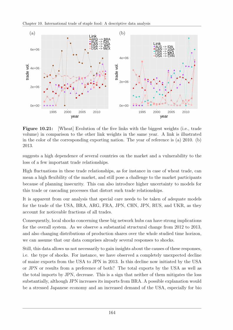
Chapter 10. International trade of staple food: A descriptive data analysis
0e+00
2e+06
4e+06
6e+06
1995 2000 2005 2010year
trad
e vo
l.
Link ARG −> BRAAUS −> IDNCAN −> USAUSA −> JPNUSA −> MEX
0e+00
2e+06
4e+06
1995 2000 2005 2010year
trad
e vo
l.
Link AUS −> IDNCAN −> USAFRA −> DZAUSA −> BRAUSA −> CHN
(a) (b)
Figure 10.21: [Wheat] Evolution of the five links with the biggest weights (i.e., tradevolume) in comparison to the other link weights in the same year. A link is illustratedin the color of the corresponding exporting nation. The year of reference is (a) 2010. (b)2013.
suggests a high dependence of several countries on the market and a vulnerability to the
loss of a few important trade relationships.
High fluctuations in these trade relationships, as for instance in case of wheat trade, can
mean a high flexibility of the market, and still pose a challenge to the market participants
because of planning insecurity. This can also introduce higher uncertainty to models for
this trade or cascading processes that distort such trade relationships.
It is apparent from our analysis that special care needs to be taken of adequate models
for the trade of the USA, BRA, ARG, FRA, JPN, CHN, JPN, RUS, and UKR, as they
account for noticeable fractions of all trades.
Consequently, local shocks concerning these big network hubs can have strong implications
for the overall system. As we observe a substantial structural change from 2012 to 2013,
and also changing distributions of production shares over the whole studied time horizon,
we can assume that our data comprises already several responses to shocks.
Still, this data allows us not necessarily to gain insights about the causes of these responses,
i.e. the type of shocks. For instance, we have observed a completely unexpected decline
of maize exports from the USA to JPN in 2013. Is this decline now initiated by the USA
or JPN or results from a preference of both? The total exports by the USA as well as
the total imports by JPN, decrease. This is a sign that neither of them mitigates the loss
substantially, although JPN increases its imports from BRA. A possible explanation would
be a stressed Japanese economy and an increased demand of the USA, especially for bio
164

10.9. Discussion
fuel production. A hint supporting this hypothesis is an increase in prices that American
farmers receive for their products - also in relation to producers in other countries. Thus,
the value of Maize seems to increase for the USA and might be less affordable by JPN.
By this example, we see that detailed analysis of several hypotheses and their coherence
with the data is required to infer causal responses to shocks. This is only possible for
a limited number of cases and cannot incorporate scenarios that do not follow the trend
observed in the data before. We discuss this problem further in Chap. 12, where we take
several steps towards a more realistic cascade model.
Considering the uncertainty about the decisions of all economic actors and possible shock
scenarios, it is reasonable to start first with a simple cascade model that can reveal already
some basic trends and economic food dependencies that go beyond the analysis of network
neighbors and incorporate more topological features of the network patterns.
Such a model needs to make strong assumptions on the causal propagation of shocks. We
motivate those assumptions by economic arguments and show how they lead to an OLRD
type cascade model in the next chapter.
165

Chapter 11
Overload redistribution: A
dependency analysis for international
trade of staple food
Summary
We introduce an OLRD type cascade model that can be interpreted as propa-gation of export bans in a weighted and directed economic network. Its impli-cations for the international trade of maize, rice, soy, and wheat are comparedwith respect to two different shock scenario types.
In our analysis, we investigate economic trade dependencies that go beyond theidentification of direct trade relationships. In contrast to our previous studies,we encounter a temporal dimension with the yearly evolution of systemic risk.For the identification of basic trends, we complement the average fraction offailed nodes by several indicators that measure additional aspects of the cascadeprocess. Most information is carried by the average fraction of trade that iswithdrawn in response to shocks. It serves especially well in the identificationof trade intermediary countries and gives thus rise to a cascade betweennesscentrality.
Our simple model is limited in its ability to estimate systemic risk, whencountries have the option to increase imports instead of solely reducing theirexports. However, it gives valuable information about the role of countries ininternational trade of staple food.
Furthermore, it is our first step towards a more refined cascade model.
RB wrote this chapter specifically for this thesis. RB designed the research questions, contributed todiscussions, derived the formulas, wrote the code and performed the analysis.
167
Chapter 11. Overload redistribution: A dependency analysis for international trade of staple food
11.1 Introduction
In the previous chapter, we have explored several topological features of four different
temporal networks, where each belongs to the yearly evolution of international trade rela-
tionships between 176 world countries with respect to one of the four major internationally
traded crops: maize, rice, soy, and wheat.
There, we have restricted ourselves to the analysis of direct trade relationships by the
comparison of link weight distributions and the identification of major exporters and
importers.
Usually, further information is not taken into account in an economic analysis of trade
dependencies. But further topological features of a network can become relevant, as the
interconnectivity and market dependency grow, because the system can become more
prone to cascades. Thus, local changes in another part of the world can impact a country,
although there is no direct trade link.
For a detailed and realistic risk scenario analysis, we would need to understand the forces
and mechanisms that lead to the formation of trades. This would require more informa-
tion than is accessible or possible to include in a small computable model. For instance,
multilateral and bilateral trade agreements in relation to tariffs, all kinds of direct and
indirect subsidies or other economic dependencies affect the attractiveness of a trade part-
ner. Moreover, the time of harvests and thus the relation of supply and demand in a year
shape the aggregated links that we consider and might lead to surprises on the aggregated
level. But also factors like cultural similarity, geographic proximity, or simply a historic
path dependence and the experience of past successful trades can influence economic deci-
sions. Those human decisions do not need to be rational or just consider less information
or more information than we have available. In summary, our subject of interest is a
complex system that we cannot model in detail.
Still, we capture many of the processes that have shaped it indirectly. The idea is that
these processes are reflected in the network topology indirectly and small distortions in
some (exogenous) variables cause a reorganization of the network that starts from the
originally observed one. This reorganization we describe by a cascade process.
For instance, a country whose production has decreased or demand has increased might
seek for a compensation of its deficit by increasing its imports or decreasing its exports.
Thus, every otherwise established trade link in a network is questioned, and might be
partially redirected to the shocked country. This redirection causes a decline of imports
for other countries and creates thus another shock that might further propagate through
the network and successively change the network topology of international trades. In
principle, the competition with other trade links might not only have local implications,
but can also impact the global market, e.g., lead to price increases, and thus introduce
168
11.1. Introduction
systemic feedback to a cascade model.
With and without systemic feedback, we implicitly assume a memory of old trade relation-
ships and high stability in the rules that lead to the formation of trade links. Furthermore,
our modeling approach is only reasonable, if the variables that are changed in a shock sce-
nario only cause negligible changes in the processes that we do not observe but that shape
the network topology.
Consequently, smaller shocks should be better represented by our model than large shocks,
as extreme scarcity of food supply probably changes substantially the behavior of all af-
fected economic agents. Especially extreme scenarios are difficult to study, as data is
hardly available for these cases. Puma et al. (2015) assume, for instance, that shocked
countries discard completely their exports and reallocate oversupplies according to a gdp
ranking of possible trade partners. Thus, the network topology, traditional trade relation-
ships, or other political considerations, are almost irrelevant in their model. Meanwhile,
Sartori and Schiavo (2015) discuss the weighted and unweighted degree and second order
distribution of the virtual water trade network and link it to food security and cascading
effects without studying actual cascades. Nevertheless, systemic risk and the result of cas-
cade processes depend crucially on details of the microscopic topology. By incorporating
such features, we thus advance our systemic risk analysis further.
In this chapter, we focus on a simple OLRD-type cascade model that describes the evolu-
tion of export restrictions of shocked countries. Export bans are not an unusual instrument
to ensure the food supply of the population, especially considering the trade of rice (Gior-
dani et al., 2014; Puma et al., 2015). Although the adjustment of imports might be an
additional option, we restrict our analysis at this point to the more extreme case, where
imports cannot be increased.
Our general approach to study the response of a network to small distortions as cascade
could have several use cases. First, it provides a way to test the implications of hypothetical
shocks on the production or demand side in several risk scenarios. Second, it can be
interpreted as part of descriptive topological data analysis to judge the trade coreness or
centrality of nodes in the trade network. Third, in principle the model could be employed
for the prediction of future trade networks on the basis of past observed trade relationships
and expected future production amounts of countries. But this would require a more
complicated and detailed cascade modeling ansatz than we can provide in this thesis.
Still, this might be a goal of future research.
Here, we restrict ourselves to a simple dependency analysis between countries that incor-
porates cascade effects and goes beyond an analysis of direct neighbors, as it incorporates
the topology of the complete observed network topology.
169
Chapter 11. Overload redistribution: A dependency analysis for international trade of staple food
11.2 A cascade model for cascading export restric-
tions
As we shift our attention to the application of international food trade, we need to extend
our interpretation of a node’s state si(t) in a cascade process and consequently reflect on
our earlier measure of systemic risk.
In Part I and II, we have assumed that si can only switch from functional (si = 0) to
failed (si = 1), but not vice versa. Next, we also allow for the (partial) recovery of node
by canceling exports. Such a recall of exports we associate with an overload redistribution
similarly to our models in Part I of this thesis.
We thus define the threshold θi of a node i as its original demand
θi := demi(0) = prodi(0) + impi(0)− expi(0)
in a non-shocked network at time t = 0 (which does not change in this chapter due to
price changes taking the price elasticity of a country’s population into consideration). As
before, the threshold stays constant the whole cascade over, which evolves according to
discrete time steps t = 0, · · · , T . This time scale is different from the yearly evolution of
the food trade networks that is measured in y. A complete cascade is assumed to develop
in each single year and defines in its end state at time T a new trade network as result of
a distortion of the originally observed one.
The load λi(t) that a node carries depends on the cascade time t and is defined by the
deficit of food in the country in comparison to its demand. This deficit can either be
caused by an initial shock to the production or demand of a country or result from an
export reduction by in-neighbors, which could not be compensated fully (yet). We define
λi(t) as amount of staple food present in a country:
λi(t) = prodi(t)− expi(t) + impi(t)− shocki. (11.1)
Here, shocki denotes the initial shock size that a country is exposed to. To emphasize that
it refers to an additional exogenous variable that is to be defined, it is as separate summand
in our definition of λi(t), although it formally decreases the already considered production
of a country or increases the demand (so technically the threshold) of a country.
If λi(t) < θi, the state of node i is defined as active (or former failed) in the next time
step: si(t+ 1) = 1. Thus, a similar relation
si(t+ 1) = H (θi − λi(t))
holds as before, where H denotes the Heaviside function. However, the failure of a node
170

11.2. A cascade model for cascading export restrictions
does not occur when its threshold is exceeded as in our previous investigations. Instead,
a node i is activated (fails) when its load λi becomes smaller than its threshold (λi < θi).1
An additional difference to our previous assumptions is that when a node distributes load
it reduces also the load λi that it carries and thus supports its recovery. When a node
is active at t + 1 (si(t + 1) = 1) it diminishes as many of its exports as necessary to
compensate for its supply deficit, if this is feasible. Thus, it tries to call back in total
li(t+ 1) = θi− λi(t+ 1). If all of its exports are not enough to recover fully from a shock,
it tries to minimize its deficit and simply calls back everything that is possible. We thus
have li(t+ 1) = min (θi − λi(t+ 1), expi(t)). The exports that are left are therefore:
expi(t + 1) = expi(t)− li(t + 1) = expi(t)−min (θi − λi(t + 1), expi(t)) .
In the next time step, the load that a node carries λi(t + 1) is updated according to
Equ. (11.1). If the compensation has been successful (i.e. λi(t + 2) = θi), the considered
node recovers fully and its state switches back to fully supplied (or functional) (si(t+ 2) =
0).
We still need to specify how the neighbors of a node are affected by the withdrawal of
exports. At this point, we assume that a country has no preference for trading partners
and wants to displease each of them as little as possible. Thus, the proportions of exports
to each country in comparison to the others are kept constant. Let wji(t) denote the
quantity of exports of a given crop (c) from country j to country i in given year y at time
t in a cascade process. Thus, we have wji(0) ∈ W (c)(y) as defined in Ch. 10. From our
assumption follows that we update in each time step the exports from an active country
by
wji(t+ 1) = wji(t)−wji(0)
expj(0)lj(t+ 1)sj(t+ 1),
where we always have∑N
j=1wji(0)
expj(0)= 1. As consequence, the imports by each country
might be reduced because of export reductions by in-neighbors in the network:
impi(t+ 1) = impi(t)−N∑j=1
wji(0)
expj(0)lj(t+ 1)sj(t+ 1).
Additional to the nodes’ state variables, the changing weights, exports, and imports carry
interesting information about the extend of the countries’ exposure to the studied cascade
processes. Because of this, we accompany our previous measure - the final cascade size,
1Remark: We could still fit the definition of θi and λi in our previous framework by setting θi = 0for all nodes and λi(t) = demi − prodi(t) − impi(t) + expi(t), i.e., the loss of food with respect to theirdemand. As this would hide the heterogeneity of demands and possible losses, we favor the definitionabove.
171
Chapter 11. Overload redistribution: A dependency analysis for international trade of staple food
which corresponds here to the fraction of countries with a supply deficit - by several other
measures that are introduced next.
11.3 Measures of systemic risk
By turning our attention to an application, we have to broaden our understanding of
systemic risk and need to be able to consider several aspects in our analysis.
The fraction %(c) of countries with a supply deficit of a specific crop c gives information
about the outreach of a cascade, but does not allow to judge the deepness of deficits
that the affected countries face. For instance, a high number could pinpoint to a good
diversification of a shock among many countries so that each of them faces only little
deficits. On the contrary, it could also be interpreted as problematic, since a considerable
number of countries is affected that cannot compensate for the loss by other means, e.g.,
substituting food types.
We need to incorporate further information about the affected countries to judge about
the deepness of a food deficit. Because of this, we complement %(c) by several additional
indicators.
The total unfulfilled demand is not indicative, because it coincides with the shock size
that we define and it does not relate it to a country’s perception of its deficit. Because
of this, we report additionally to %(c) the percentage at which a country’s demand is not
fulfilled and weight it by their amount of population. Finally, we calculate the percentage
of world population whose original demand is not met and term it δ (for deficit):
δ(c)(y) :=1
popTot(y)
N∑i=1
θ(c)i − λ
(c)i (T )
dem(c)i
popi(y).
This measure can only be a proxy for a change in actual food deficit in comparison to
an observed distribution. It does neither question the observed distribution nor does it
consider that the demand is not equally distributed between the inhabitants of a country
or that a significant percentage of the demand might not be used for human consumption
at all. In general, the change in demand of a country with relatively high demand despite
a small population is weighted less than the change in demand of a country with high pop-
ulation and relatively low demand. More advanced measures might be worth considering
in future that incorporate information about the food insecurity of countries.
Furthermore, even if a country does not face a deficit at the end of a cascade, a combined
reduction of imports and exports might still have negative consequences. For instance, the
value added by the country to a product may be lost. Or, the benefit from the time gap
between the own export and the import may be lost. This benefit could result from profits
172
11.4. Shock scenarios
of selling when the price is high and buying when the price is lower, or it could mean a
saving of stocking costs in the time when the specific staple is not needed. Moreover, the
exported crop quality could be lower than the imported one. We have made the simplifying
assumption that all trades referring to a specific crop correspond to the same type of crop
of the same quality. But it might not be possible to use all traded goods for the same
purpose. Because of this, we also measure the amount of trade distortion as result of a
cascade. We thus consider as third measure the fraction of all export changes
ε(c)(y) :=1
expTot(c)(y)
N∑i=1
(exp
(c)i (0)− exp
(c)i (T)
),
where expTot(c)(y) denotes the sum of all originally observed trades: expTot(c)(y) =∑Ni=1 exp
(c)i (0). The extend to which a node has to readjust its exports can also be inter-
preted as its coreness or betweenness with respect to trades. A high amount of adjusted
exports means that a node is involved many times or to substantial amounts in a cascade.
Thus, it might lie on many possible ‘cascade paths’ between nodes.
%(c), δ(c), and ε(c) are the most important measures that we consider. Additionally, we
report the time T (c) until a cascade reaches its steady state and the total number N(c)er of
export reduction events to judge how fast and how broad a cascade evolves. Both inform
about the feasibility of possible interventions.
11.4 Shock scenarios
The modeling of realistic shock scenarios is a challenge on its own that we cannot discuss
in depth in this thesis. Shocks can originate from natural hazards, weather anomalies,
pests, increasing wastes, etc on the production side or from increasing demands because
of additional crop usage possibilities, speculation, or simply increasing population, etc. Of
course, also the transportation of goods could face shocks, but this is not considered in
this thesis.
Here, we focus on cascade effects resulting from trade interdependencies between countries.
Consequently, we are mainly interested in the hypothetical question how a country i is
affected in case of a shock originating in another country j. For this purpose, we study N
different shock scenarios in each of which a single country j is shocked.
Shock 1. In the first scenario, each country i is shocked by the same amount sa. We
simply choose sa(c)(y) = 0.25 prodTot(c)(y)/N, i.e., 25% of the average production by a
country, because at least 5% of all shocks in our data are this severe. If the demand and
the production of a country are smaller than sa(c)(y) we assume that the shock is only of
the size of the maximum of both. This ensures that we do not assume that a country’s
173
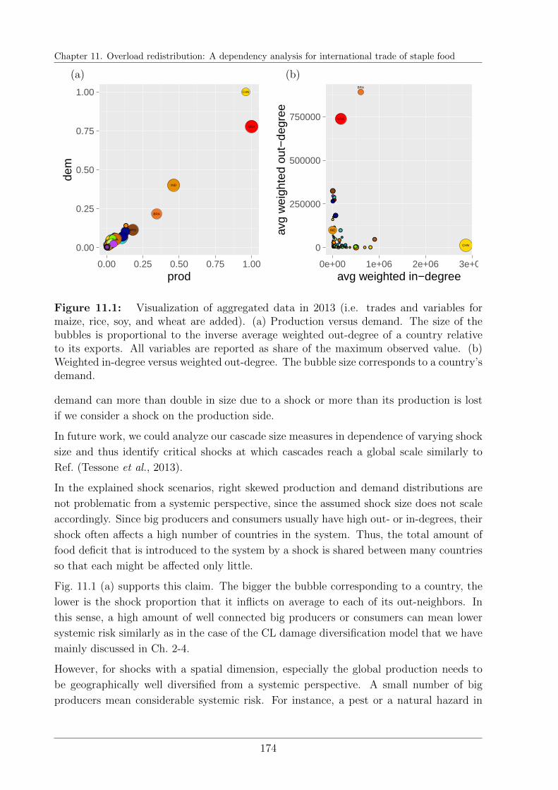
Chapter 11. Overload redistribution: A dependency analysis for international trade of staple food
USA
ARG
BRA
CHN
IND
THA
0.00
0.25
0.50
0.75
1.00
0.00 0.25 0.50 0.75 1.00prod
dem
USA
BRA
CHN
IND
0
250000
500000
750000
0e+00 1e+06 2e+06 3e+06avg weighted in−degree
avg
wei
ghte
d ou
t−de
gree
(a) (b)
Figure 11.1: Visualization of aggregated data in 2013 (i.e. trades and variables formaize, rice, soy, and wheat are added). (a) Production versus demand. The size of thebubbles is proportional to the inverse average weighted out-degree of a country relativeto its exports. All variables are reported as share of the maximum observed value. (b)Weighted in-degree versus weighted out-degree. The bubble size corresponds to a country’sdemand.
demand can more than double in size due to a shock or more than its production is lost
if we consider a shock on the production side.
In future work, we could analyze our cascade size measures in dependence of varying shock
size and thus identify critical shocks at which cascades reach a global scale similarly to
Ref. (Tessone et al., 2013).
In the explained shock scenarios, right skewed production and demand distributions are
not problematic from a systemic perspective, since the assumed shock size does not scale
accordingly. Since big producers and consumers usually have high out- or in-degrees, their
shock often affects a high number of countries in the system. Thus, the total amount of
food deficit that is introduced to the system by a shock is shared between many countries
so that each might be affected only little.
Fig. 11.1 (a) supports this claim. The bigger the bubble corresponding to a country, the
lower is the shock proportion that it inflicts on average to each of its out-neighbors. In
this sense, a high amount of well connected big producers or consumers can mean lower
systemic risk similarly as in the case of the CL damage diversification model that we have
mainly discussed in Ch. 2-4.
However, for shocks with a spatial dimension, especially the global production needs to
be geographically well diversified from a systemic perspective. A small number of big
producers mean considerable systemic risk. For instance, a pest or a natural hazard in
174
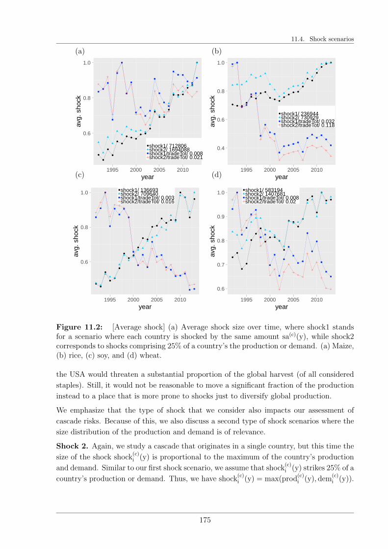
11.4. Shock scenarios
0.6
0.8
1.0
1995 2000 2005 2010year
avg.
sho
ck
shock1/ 712806shock2/ 1694088shock1/tradeTot/ 0.008shock2/tradeTot/ 0.021
0.4
0.6
0.8
1.0
1995 2000 2005 2010year
avg.
sho
ck
shock1/ 236944shock2/ 730929shock1/tradeTot/ 0.032shock2/tradeTot/ 0.118
0.6
0.8
1.0
1995 2000 2005 2010year
avg.
sho
ck
shock1/ 136693shock2/ 709640shock1/tradeTot/ 0.003shock2/tradeTot/ 0.016
0.6
0.7
0.8
0.9
1.0
1995 2000 2005 2010year
avg.
sho
ck
shock1/ 583194shock2/ 1407681shock1/tradeTot/ 0.008shock2/tradeTot/ 0.02
(a) (b)
(c) (d)
Figure 11.2: [Average shock] (a) Average shock size over time, where shock1 standsfor a scenario where each country is shocked by the same amount sa(c)(y), while shock2corresponds to shocks comprising 25% of a country’s the production or demand. (a) Maize,(b) rice, (c) soy, and (d) wheat.
the USA would threaten a substantial proportion of the global harvest (of all considered
staples). Still, it would not be reasonable to move a significant fraction of the production
instead to a place that is more prone to shocks just to diversify global production.
We emphasize that the type of shock that we consider also impacts our assessment of
cascade risks. Because of this, we also discuss a second type of shock scenarios where the
size distribution of the production and demand is of relevance.
Shock 2. Again, we study a cascade that originates in a single country, but this time the
size of the shock shock(c)i (y) is proportional to the maximum of the country’s production
and demand. Similar to our first shock scenario, we assume that shock(c)i (y) strikes 25% of a
country’s production or demand. Thus, we have shock(c)i (y) = max(prod
(c)i (y), dem
(c)i (y)).
175
Chapter 11. Overload redistribution: A dependency analysis for international trade of staple food
For both shock scenario types, we calculate the introduced systemic risk measures for each
shock on a country and report then the mean quantity of all single country shocks.
11.5 Cascade results
The interpretation of our cascade analysis results depends crucially on a reader’s per-
ception of international market dependence. Systemic risk studies usually emphasize the
drawbacks of interconnectivity and interdependence. Certainly, collateral costs of trans-
portation for the environment are a negative externality. The dependence on volatile
markets, unreliable trade partners, or unforeseen shocks in another part of the world are
examples for problems that can come along with globalization.
Nevertheless, international trade has also many advantages for the engaging countries,
as already discussed earlier. In relation to food, it enables varied diets (for people who
can afford it) and allow for specialization, which can lead to more efficient production.
Also from a risk perspective, trade offers the opportunity to mitigate harvest losses or
compensate for a scarcity of farming resources. Thus, autarky as alternative to imports
might not be an option for many countries. Still, the degree of dependence on the market
and on other countries can be partially regulated and is an important information for
policy makers or trade participants.
Because of this, we provide first steps in the identification of trade interdependencies taking
cascade effects into account, which serve as model for the response of the international
trade network to shocks.
11.5.1 Relations of interdependencies
Differences in shock scenarios
Fig. 11.3 shows our results for the international trade of maize in 2010: a network of trade
interdependencies. Each shock of a single country is represented by the links leaving the
corresponding node, which are colored according to the shocked node. The link weight is
proportional to the demand deficit at the end of the studied cascade of a node where the
link points to. The demand deficit that a shocked node faces on its own is not shown.
Shock 1. In case that each node is shocked initially by the same amount, as illustrated
by Fig. 11.3 (a), we observe a relatively good diversification of shocks starting in main
exporters. One exception is the high exposure of KOR towards CHN and ESP is hit by
cascades in many cases.
Still, in comparison with our second shock scenario where countries are shocked propor-
tional to their production or demand, shocks are well shared among international countries.
176
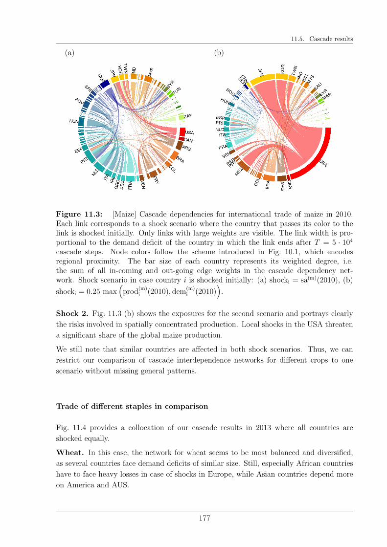
11.5. Cascade results
(a) (b)
Figure 11.3: [Maize] Cascade dependencies for international trade of maize in 2010.Each link corresponds to a shock scenario where the country that passes its color to thelink is shocked initially. Only links with large weights are visible. The link width is pro-portional to the demand deficit of the country in which the link ends after T = 5 · 104
cascade steps. Node colors follow the scheme introduced in Fig. 10.1, which encodesregional proximity. The bar size of each country represents its weighted degree, i.e.the sum of all in-coming and out-going edge weights in the cascade dependency net-work. Shock scenario in case country i is shocked initially: (a) shocki = sa(m)(2010), (b)
shocki = 0.25 max(
prod(m)i (2010), dem
(m)i (2010)
).
Shock 2. Fig. 11.3 (b) shows the exposures for the second scenario and portrays clearly
the risks involved in spatially concentrated production. Local shocks in the USA threaten
a significant share of the global maize production.
We still note that similar countries are affected in both shock scenarios. Thus, we can
restrict our comparison of cascade interdependence networks for different crops to one
scenario without missing general patterns.
Trade of different staples in comparison
Fig. 11.4 provides a collocation of our cascade results in 2013 where all countries are
shocked equally.
Wheat. In this case, the network for wheat seems to be most balanced and diversified,
as several countries face demand deficits of similar size. Still, especially African countries
have to face heavy losses in case of shocks in Europe, while Asian countries depend more
on America and AUS.
177

Chapter 11. Overload redistribution: A dependency analysis for international trade of staple food
(a) (b)
(c) (d)
Figure 11.4: Cascade dependencies in 2013. Each link corresponds to a shock scenariowhere the country that passes its color to the link is shocked initially by sa(c)(y) as definedin Sec. 11.4. The link width is proportional to the demand deficit of the country in whichthe link ends after T = 5 · 104 cascade steps. Node colors follow the scheme introduced inFig. 10.1, which encodes regional proximity. The bar size of each country represents itsweighted degree, i.e. the sum of all in-coming and out-going edge weights in the cascadedependency network. Considered staples: (a) maize, (b) rice, (c) soy, and (d) wheat.
Maize. A similar tendency can be observed for maize. Noticeably, MEX and VEN are
relatively dependent on the USA despite their own maize productions.
Rice. In case of rice trade, Asia and the USA are clearly crucial for the world supply. In
particular African countries rely on Asian exports. Also KOR and JPN as Asian countries
are highly dependent, mostly on CHN and the USA.
178
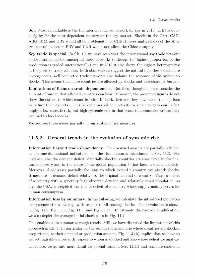
11.5. Cascade results
Soy. Most remarkable is the the interdependence network for soy in 2013. CHN is obvi-
ously by far the most dependent country on the soy market. Shocks in the USA, CAN,
ARG, BRA and URY would all be problematic for CHN. Interestingly, shocks of the other
two central exporters PRY and UKR would not affect the Chinese supply.
Soy trade is special. In Ch. 10, we have seen that the international soy trade network
is the least connected among all trade networks (although the highest proportion of the
production is traded internationally) and in 2013 it also shows the highest heterogeneity
in the positive trade volumes. Both observations suggest the natural hypothesis that more
homogeneous, well connected trade networks also balance the response of the system to
shocks. This means that more countries are affected by shocks and also share its burden.
Limitations of focus on trade dependencies. But these thoughts do not consider the
amount of burden that affected countries can bear. Moreover, the presented figures do not
show the extend to which countries absorb shocks because they have no further options
to reduce their exports. Thus, a low observed connectivity or small weights can in fact
imply a low cascade risk, but high systemic risk in that sense that countries are severely
exposed to local shocks.
We address these issues partially in our systemic risk measures.
11.5.2 General trends in the evolution of systemic risk
Information beyond trade dependency. The discussed aspects are partially reflected
in our one-dimensional indicators, i.e., the risk measures introduced in Sec. 11.3. For
instance, also the demand deficit of initially shocked countries are considered in the final
cascade size % and in the share of the global population δ that faces a demand deficit.
Moreover, δ addresses partially the issue to which extend a country can absorb shocks.
It measures a demand deficit relative to the original demand of country. Thus, a deficit
of a country with a generally high observed demand and relatively small population, as
e.g. the USA, is weighted less than a deficit of a country whose supply mainly serves for
human consumption.
Information loss by summary. In the following, we calculate the introduced indicators
for systemic risk as average with respect to all country shocks. Their evolution is shown
in Fig. 11.5, Fig. 11.7, Fig. 11.9, and Fig. 11.11. To estimate the cascade amplification,
we also depict the average initial shock sizes in Fig. 11.2.
This enables us to summarize rough trends. Still, we have discussed the limitations of this
approach in Ch. 9. In particular for the second shock scenario where countries are shocked
proportional to their demand or production amount, Fig. 11.3 (b) implies that we have to
expect high differences with respect to whom is shocked and also whose deficit we analyze.
Therefore, we go into more detail for special cases in Sec. 11.5.3 and compare shocks of
179
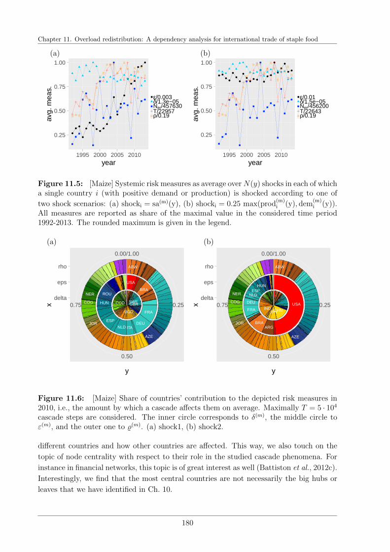
Chapter 11. Overload redistribution: A dependency analysis for international trade of staple food
0.25
0.50
0.75
1.00
1995 2000 2005 2010year
avg.
mea
s.
ε/0.003δ/1.3e−05Ner/457630T/22957ρ/0.19
0.25
0.50
0.75
1.00
1995 2000 2005 2010year
avg.
mea
s.
ε/0.01δ/1.5e−05Ner/456200T/22643ρ/0.19
(a) (b)
Figure 11.5: [Maize] Systemic risk measures as average overN(y) shocks in each of whicha single country i (with positive demand or production) is shocked according to one of
two shock scenarios: (a) shocki = sa(m)(y), (b) shocki = 0.25 max(prod(m)i (y), dem
(m)i (y)).
All measures are reported as share of the maximal value in the considered time period1992-2013. The rounded maximum is given in the legend.
BGD
SWEGBRCOD
FRA
DEUESP
NLD
USA
BRA
ITA
ROU
HUN
NER
COG
ABW
AZE
JOR
0.25
0.50
0.75
0.00/1.00
delta
eps
rho
y
x
CHNINDJPN
USA
BRAARG
FRA
DEU
ESPNLD
HUN
NER
COG
ABW
AZE
JOR
0.25
0.50
0.75
0.00/1.00
delta
eps
rho
y
x
(a) (b)
Figure 11.6: [Maize] Share of countries’ contribution to the depicted risk measures in2010, i.e., the amount by which a cascade affects them on average. Maximally T = 5 · 104
cascade steps are considered. The inner circle corresponds to δ(m), the middle circle toε(m), and the outer one to %(m). (a) shock1, (b) shock2.
different countries and how other countries are affected. This way, we also touch on the
topic of node centrality with respect to their role in the studied cascade phenomena. For
instance in financial networks, this topic is of great interest as well (Battiston et al., 2012c).
Interestingly, we find that the most central countries are not necessarily the big hubs or
leaves that we have identified in Ch. 10.
180
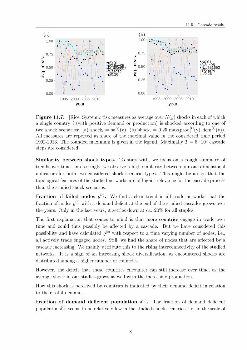
11.5. Cascade results
0.00
0.25
0.50
0.75
1.00
1995 2000 2005 2010year
avg.
mea
s.
ε/0.01δ/2.5e−05Ner/650007T/23079ρ/0.26
0.00
0.25
0.50
0.75
1.00
1995 2000 2005 2010year
avg.
mea
s.
ε/0.01δ/2e−05Ner/651653T/23079ρ/0.26
(a) (b)
Figure 11.7: [Rice] Systemic risk measures as average over N(y) shocks in each of whicha single country i (with positive demand or production) is shocked according to one of
two shock scenarios: (a) shocki = sa(r)(y), (b) shocki = 0.25 max(prod(r)i (y), dem
(r)i (y)).
All measures are reported as share of the maximal value in the considered time period1992-2013. The rounded maximum is given in the legend. Maximally T = 5 · 104 cascadesteps are considered.
Similarity between shock types. To start with, we focus on a rough summary of
trends over time. Interestingly, we observe a high similarity between our one-dimensional
indicators for both two considered shock scenario types. This might be a sign that the
topological features of the studied networks are of higher relevance for the cascade process
than the studied shock scenarios.
Fraction of failed nodes %(c). We find a clear trend in all trade networks that the
fraction of nodes %(c) with a demand deficit at the end of the studied cascades grows over
the years. Only in the last years, it settles down at ca. 20% for all staples.
The first explanation that comes to mind is that more countries engage in trade over
time and could thus possibly be affected by a cascade. But we have considered this
possibility and have calculated %(c) with respect to a time varying number of nodes, i.e.,
all actively trade engaged nodes. Still, we find the share of nodes that are affected by a
cascade increasing. We mainly attribute this to the rising interconnectivity of the studied
networks. It is a sign of an increasing shock diversification, as encountered shocks are
distributed among a higher number of countries.
However, the deficit that these countries encounter can still increase over time, as the
average shock in our studies grows as well with the increasing production.
How this shock is perceived by countries is indicated by their demand deficit in relation
to their total demand.
Fraction of demand deficient population δ(c). The fraction of demand deficient
population δ(c) seems to be relatively low in the studied shock scenarios, i.e. in the scale of
181
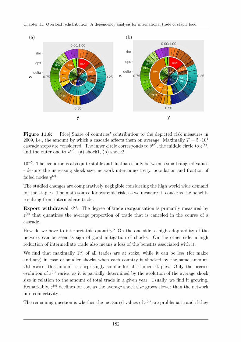
Chapter 11. Overload redistribution: A dependency analysis for international trade of staple food
MEX
RUS
USATHA
PAK BRA
IND
ITA
URYCHN
ZWE
RWABFA
GHA
YEM
0.25
0.50
0.75
0.00/1.00
delta
eps
rho
y
x
MEX
RUS
THA
USA
PAKINDCHN
BRA
ITADEU
ZWE
RWABFA
GHA
YEM
CPV
0.25
0.50
0.75
0.00/1.00
delta
eps
rho
yx
(a) (b)
Figure 11.8: [Rice] Share of countries’ contribution to the depicted risk measures in2009, i.e., the amount by which a cascade affects them on average. Maximally T = 5 · 104
cascade steps are considered. The inner circle corresponds to δ(r), the middle circle to ε(r),and the outer one to %(r). (a) shock1, (b) shock2.
10−5. The evolution is also quite stable and fluctuates only between a small range of values
- despite the increasing shock size, network interconnectivity, population and fraction of
failed nodes %(c).
The studied changes are comparatively negligible considering the high world wide demand
for the staples. The main source for systemic risk, as we measure it, concerns the benefits
resulting from intermediate trade.
Export withdrawal ε(c). The degree of trade reorganization is primarily measured by
ε(c) that quantifies the average proportion of trade that is canceled in the course of a
cascade.
How do we have to interpret this quantity? On the one side, a high adaptability of the
network can be seen as sign of good mitigation of shocks. On the other side, a high
reduction of intermediate trade also means a loss of the benefits associated with it.
We find that maximally 1% of all trades are at stake, while it can be less (for maize
and soy) in case of smaller shocks when each country is shocked by the same amount.
Otherwise, this amount is surprisingly similar for all studied staples. Only the precise
evolution of ε(c) varies, as it is partially determined by the evolution of the average shock
size in relation to the amount of total trade in a given year. Usually, we find it growing.
Remarkably, ε(c) declines for soy, as the average shock size grows slower than the network
interconnectivity.
The remaining question is whether the measured values of ε(c) are problematic and if they
182
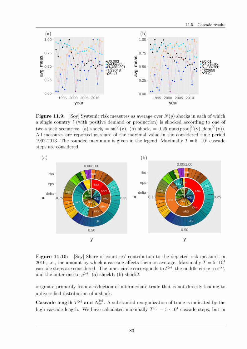
11.5. Cascade results
0.00
0.25
0.50
0.75
1.00
1995 2000 2005 2010year
avg.
mea
s.
ε/0.003δ/4.8e−05Ner/382391T/23048ρ/0.21
0.00
0.25
0.50
0.75
1.00
1995 2000 2005 2010year
avg.
mea
s.
ε/0.01δ/4.7e−05Ner/387891T/22658ρ/0.21
(a) (b)
Figure 11.9: [Soy] Systemic risk measures as average over N(y) shocks in each of whicha single country i (with positive demand or production) is shocked according to one of
two shock scenarios: (a) shocki = sa(s)(y), (b) shocki = 0.25 max(prod(s)i (y), dem
(s)i (y)).
All measures are reported as share of the maximal value in the considered time period1992-2013. The rounded maximum is given in the legend. Maximally T = 5 · 104 cascadesteps are considered.
POLPAK
NGA
NLD
USA
BRA
CAN
PRY
ARG
CHN
MUS
FIN
IDN
LTU
JOR
BRB
0.25
0.50
0.75
0.00/1.00
delta
eps
rho
y
x POLPAK
NGAUSA
BRA
ARG
NLDPRY
CAN
CHN
MUS
FIN
IDN
LTU
JOR
BRB
0.25
0.50
0.75
0.00/1.00
delta
eps
rho
y
x
(a) (b)
Figure 11.10: [Soy] Share of countries’ contribution to the depicted risk measures in2010, i.e., the amount by which a cascade affects them on average. Maximally T = 5 · 104
cascade steps are considered. The inner circle corresponds to δ(s), the middle circle to ε(s),and the outer one to %(s). (a) shock1, (b) shock2.
originate primarily from a reduction of intermediate trade that is not directly leading to
a diversified distribution of a shock.
Cascade length T (c) and N(c)er . A substantial reorganization of trade is indicated by the
high cascade length. We have calculated maximally T (c) = 5 · 104 cascade steps, but in
183

Chapter 11. Overload redistribution: A dependency analysis for international trade of staple food
several cases the cascade would continue. Only wheat trade is reorganized relatively early,
on average after ca. T (w) = 1.6 · 104 steps.
In case of all staples, the evolution of the two reported quantities is quite volatile. Espe-
cially in the first half of the observation period, we encounter big differences over orders
of magnitudes between two consecutive observations. Also T (c) and N(c)er can differ a lot
in their trend. Short cascades can still involve a high number of shock distribution events
that happen at the same time.
These can only occur, if there is a substantial fraction of intermediary countries that export
and import high amounts which can be withdrawn in the course of a cascade.
Thus, we ask next which countries are the main shock channels, along which cascades
propagate.
Cascade centrality. In the remainder, we present the figures that depict our findings
for each of the four studied staples. Alongside, we show the distribution of specific coun-
try contributions to our main systemic risk indicators %(c), δ(c), and ε(c), i.e. how these
countries are affected on average.
Our main focus is on δ(c), as this is the risk measure carrying the most interesting infor-
mation. We see that it also corresponds to the most heterogeneous distribution among
countries. A high value can further be linked to the trade centrality or cascade betweenness
of a node.
The other two distributions, relating to %(c) and δ(c), indicate a good diversification of the
cascade outcome.
Additionally, we could also depict the average systemic risk that is caused by the shock of
a country. This would identify potential cascade sources. As this question is answered to
a large extend by our economic dependency analysis, we focus on the issue how countries
are potentially affected by cascades and local shocks.
A more detailed discussion follows in the next section alongside the figures that we have
based our trend summary on. Primarily, we highlight the special characteristics concerning
each staple. The interested reader is, of course, encouraged to delve further into the results.
11.5.3 Staple characteristics
International trade of maize
Fig. 11.5 presents the evolution of the average indicators that we have introduced in
Sec. 11.3 for international trade of maize in our observation period 1992-2013. Interest-
ingly, we observe a clear growth trend in the fraction ε(m) of trade withdrawals only in
case of shock scenario 1, but not shock scenario 2. This is despite the high similarity in
184
11.5. Cascade results
the corresponding average shock evolutions as shown in Fig. 11.2 (a).
However, ε(m) is smaller in case of shock1, even though it increases. This can be expected,
as on average, the system is also shocked less. In both scenarios, the shock size is generally
increasing, although not clearly in relation to the total issued trade. For the other three
staples, the average shock decreases in relation to the total trade.
A possible indicator why we observe a relatively stable ε(m) for shock2, where countries
are shocked proportional to their production or demand, is provided in Fig. 11.6 (b). A
considerable proportion of trades is withdrawn by the USA, the main producer of Maize.
As its shock is immense in comparison to the others, this one shock scenario dominates our
average measure ε(m) to a large extend. Furthermore, each shock that reaches the USA
is distributed further to a high number of other countries which are also exporter. The
dominant role of the USA in scenario 2 is relatively stable over time. Consequently, ε(m)
does not respond strongly to structural network changes affecting our results for scenario
1.
In contrast, exports are withdrawn by the USA only to smaller extend than by several
European countries in scenario 1 as shown in Fig. 11.6 (a). This confirms our impression
of the central European role in the international trade of Maize (in addition to the USA,
BRA, and ARG).
International trade of rice
Cascades in the international trade of rice lead to the highest maximal proportion %(r) of
nodes with demand deficit as seen in Fig. 11.7. This is a sign of relatively good diversifi-
cation of shocks.
This is also apparent from Fig. 11.8, which shows that the demand deficit δ(r) is relatively
equal distributed among the countries in a similar amount shocks, as shown by their similar
contribution to %(r).
The contribution to the evolution of the export withdrawal ε(r) depends again on the
considered shock scenarios. In comparison to maize, there are more countries with a similar
contribution also in case of shock2, where countries are shocked proportional to their
production or demand. Interestingly, in scenario 2, the largest share does not correspond
to the main producers, but to one of the main exporter nations: THA. In scenario 2
instead, the biggest share does not belong to THA but to the USA.
International trade of soy
Soy is special, since we observe a decreasing trend for the share of export withdrawal ε(s)
for both shock scenarios as depicted by Fig. 11.9.
185
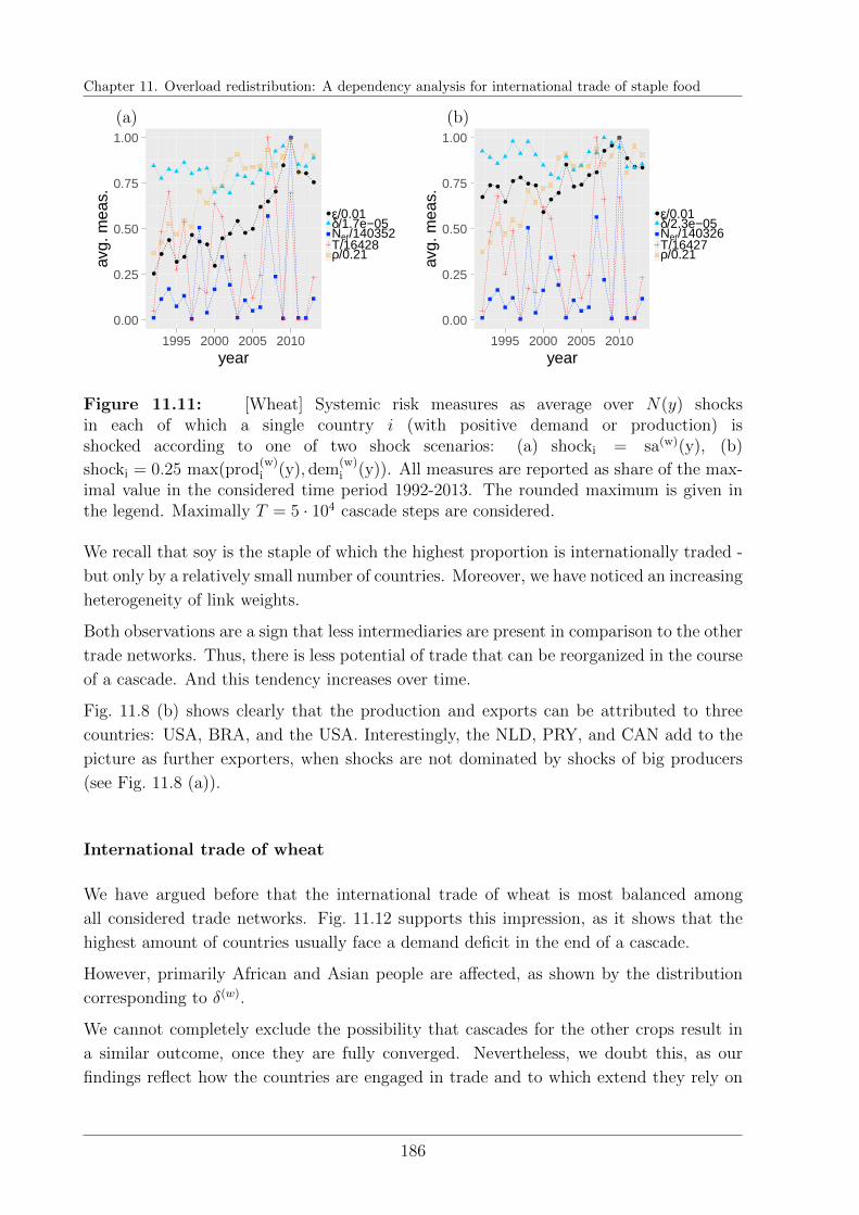
Chapter 11. Overload redistribution: A dependency analysis for international trade of staple food
0.00
0.25
0.50
0.75
1.00
1995 2000 2005 2010year
avg.
mea
s.
ε/0.01δ/1.7e−05Ner/140352T/16428ρ/0.21
0.00
0.25
0.50
0.75
1.00
1995 2000 2005 2010year
avg.
mea
s.
ε/0.01δ/2.3e−05Ner/140326T/16427ρ/0.21
(a) (b)
Figure 11.11: [Wheat] Systemic risk measures as average over N(y) shocksin each of which a single country i (with positive demand or production) isshocked according to one of two shock scenarios: (a) shocki = sa(w)(y), (b)
shocki = 0.25 max(prod(w)i (y), dem
(w)i (y)). All measures are reported as share of the max-
imal value in the considered time period 1992-2013. The rounded maximum is given inthe legend. Maximally T = 5 · 104 cascade steps are considered.
We recall that soy is the staple of which the highest proportion is internationally traded -
but only by a relatively small number of countries. Moreover, we have noticed an increasing
heterogeneity of link weights.
Both observations are a sign that less intermediaries are present in comparison to the other
trade networks. Thus, there is less potential of trade that can be reorganized in the course
of a cascade. And this tendency increases over time.
Fig. 11.8 (b) shows clearly that the production and exports can be attributed to three
countries: USA, BRA, and the USA. Interestingly, the NLD, PRY, and CAN add to the
picture as further exporters, when shocks are not dominated by shocks of big producers
(see Fig. 11.8 (a)).
International trade of wheat
We have argued before that the international trade of wheat is most balanced among
all considered trade networks. Fig. 11.12 supports this impression, as it shows that the
highest amount of countries usually face a demand deficit in the end of a cascade.
However, primarily African and Asian people are affected, as shown by the distribution
corresponding to δ(w).
We cannot completely exclude the possibility that cascades for the other crops result in
a similar outcome, once they are fully converged. Nevertheless, we doubt this, as our
findings reflect how the countries are engaged in trade and to which extend they rely on
186
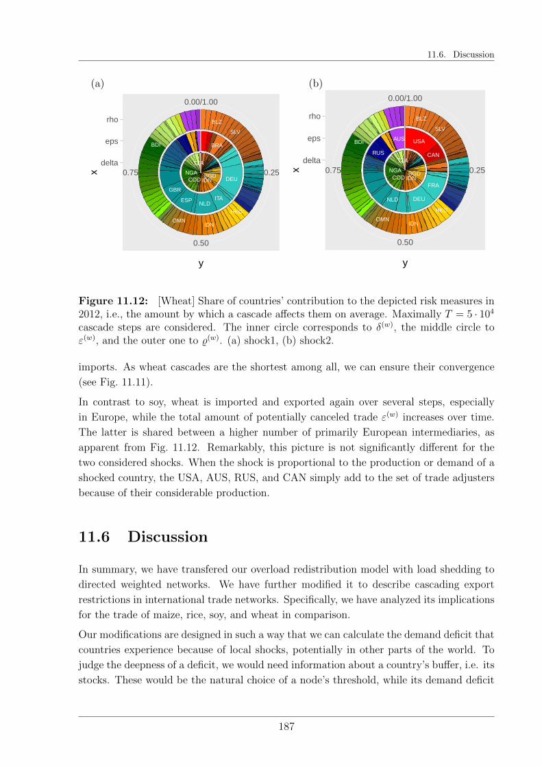
11.6. Discussion
NGA BGDIDNCOD
TZA
DEU
NLDESP ITA
GBR
BRA
HKG
IDN
BDI
OMN
BLZ
SLV
0.25
0.50
0.75
0.00/1.00
delta
eps
rho
y
x NGA BGDIDNCOD
TZA
USA
DEU
FRA
AUS
CAN
NLD
RUS
HKG
IDN
BDI
OMN
BLZ
SLV
0.25
0.50
0.75
0.00/1.00
delta
eps
rho
y
x
(a) (b)
Figure 11.12: [Wheat] Share of countries’ contribution to the depicted risk measures in2012, i.e., the amount by which a cascade affects them on average. Maximally T = 5 · 104
cascade steps are considered. The inner circle corresponds to δ(w), the middle circle toε(w), and the outer one to %(w). (a) shock1, (b) shock2.
imports. As wheat cascades are the shortest among all, we can ensure their convergence
(see Fig. 11.11).
In contrast to soy, wheat is imported and exported again over several steps, especially
in Europe, while the total amount of potentially canceled trade ε(w) increases over time.
The latter is shared between a higher number of primarily European intermediaries, as
apparent from Fig. 11.12. Remarkably, this picture is not significantly different for the
two considered shocks. When the shock is proportional to the production or demand of a
shocked country, the USA, AUS, RUS, and CAN simply add to the set of trade adjusters
because of their considerable production.
11.6 Discussion
In summary, we have transfered our overload redistribution model with load shedding to
directed weighted networks. We have further modified it to describe cascading export
restrictions in international trade networks. Specifically, we have analyzed its implications
for the trade of maize, rice, soy, and wheat in comparison.
Our modifications are designed in such a way that we can calculate the demand deficit that
countries experience because of local shocks, potentially in other parts of the world. To
judge the deepness of a deficit, we would need information about a country’s buffer, i.e. its
stocks. These would be the natural choice of a node’s threshold, while its demand deficit
187

Chapter 11. Overload redistribution: A dependency analysis for international trade of staple food
would correspond to the load that it carries. In lack of data about stocks, we assume that
they are non-existent. However, they could be easily incorporated in our model.
To capture additional aspects of the trade reorganization in response to shocks, we have
developed several indicators of systemic risk that complement the average fraction of failed
nodes, which we have focused on in the previous chapters.
We find especially the average export withdrawal a relevant measure for the degree of trade
reorganization in response to shocks. Furthermore, its definition comprises interesting
information about the cascade betweenness centrality of nodes in a network. With respect
to international trade, the most central nodes can be associated with trade intermediate
countries.
In general, we do not observe a prominent structural change in 2012/2013 in the studied
risk measures, although we have found the largest weights reorganizing in the previous
chapter. We argue that the studied shocks are not large enough to show a response. They
are much smaller than the trades along the biggest links, which are still enormous in
comparison to other trades.
However, the increasing network interconnectivity in 1992-2013 leads to an increasing
number of nodes that are finally affected by cascading export restrictions. This does not
imply that the fraction of people that face a demand deficit grows as well. In contrast,
this stays relatively stable over time. Shocks are relatively well diversified, i.e. distributed
in similar shares between a considerable number of countries, which is highest for wheat
trade.
This shock distribution process develops over a very high number of cascade time steps
and results in trade withdrawals of different size relative to the total amount of trade.
Only for soy, such trade distortions are decreasing.
This observation can be attributed to the fact that soy trade is dominated by the exports of
only three main producers and the share of intermediate trade shrinks. This is especially
problematic in case of geographically concentrated shocks that hit the main producers.
Similarly, the production of maize is not well diversified.
This limits also the possibilities to redirect imports to other producers in case of a shock.
However, this circumstance is not considered by the discussed model, as countries can
mitigate shocks only be export reduction. Imports cannot become increased or redirected,
as it would usually be the case. In this sense, we study a rather extreme shock scenario,
in which countries are not willing to export more of a scarce resource.
The advantage of our model is that the distortions preserve the observed network structure
as far as possible. In consequence, many of the hidden factors that have shaped this
structure are still considered. In this sense, we do not study such an extreme risk scenario
that the mechanisms leading to the setup of trades are completely overruled. As we are
188

11.6. Discussion
particularly interested in severe system responses to small shocks, we argue that it is a
reasonable assumption that many of the trade formation mechanisms are still in place.
Consequently, the next step towards a more realistic cascade model has to include active
decisions of shocked countries concerning their imports, as this is a realistic alternative
to export adjustments in case of small shocks. Moreover, we have to add responses on
information that is available about the system state on the macro level. The main example
for such an information is the average price of a good. Also the total production amount
might be available (or estimates thereof). A further reorganization of the network structure
might be in order in a next step. Countries value certain trades more than others and their
preferences might also be reflected in their decisions which trades they increase or decrease.
We thus have to relax our assumption that trade partners are shocked proportional to the
observed trade weight. In the next chapter, we give an outlook about possible extensions
in line with these considerations.
Although the presented scenarios are not realistic in several aspects, we still find our
model interesting because of the information that it reveals about the trade topology. As
it respects an observed network structure, it serves very well for the identification of trade
intermediary countries.
189


Chapter 12
Outlook: Towards a cascade model
tailored to the international trade of
maize
Summary
We address several unrealistic assumptions in our previous model for the tradereorganization of the international trade of staple foods as response to smallshocks. Our outline how these could be resolved includes preliminary modelinvestigations for the trade of maize.
The first step in a model improvement has to incorporate import increases aspossible strategy for countries to mitigate shocks. This requires careful mod-eling of the countries’ demands and export decisions under changed economicconditions. Furthermore, their preferences concerning their trade partners haveto be determined. Moreover their changing preferences with respect to differ-ent staples have to be considered. This would finally introduce a multiplexview.
The presented models lack predictive power yet and pose practical challenges.We discuss possible answers to these challenges and suggest solutions.
RB wrote this chapter specifically for this thesis. RB designed the research questions, contributed todiscussions, decided about the modeling, and performed the analysis.
191

Chapter 12. Outlook: Towards a cascade model tailored to the international trade of maize
12.1 Introduction
In the previous section, we have studied a simple model for cascading export restrictions
and its implications for the international trade of maize, rice, soy, and wheat. This model
comprises several assumptions that are unrealistic for our modeling purpose.
Modeling purpose. We ask how the international trade network reorganizes in response
to rather small initial shocks on the production or demand side, i.e. when countries face
bad harvests or increase their demand. This reorganization is modeled by an evolving
cascade process and thus results from local distortions of an observed trade structure for
which we create an alternative. In future, the goal is to start from networks observed in
previous years and predict trades in a given year y by cascades running on the observed
trade network in y − 1.
As reasoned in the introduction of Part III, our idea relies strongly on the assumption that
the network that we start from contains valuable information about the mechanisms that
distort it. We have to assume that these mechanisms are relatively stable. However, in an
extreme shock scenario, countries would completely reconsider their behaviour and seek
for possibilities to attain scarce resources. We could only speculate about their strategies.
Consequently, we focus on implications of small shocks on international trade of staples
that can lead already to considerable distortions of trade relationships.
Critical assumptions. The previously considered export restrictions alone signify al-
ready rather scarce resources, if they cannot be accompanied by import increases. As most
critical drawbacks of our cascade model, we regard that countries (1) are very limited in
their response strategies to a shock and (2) do not consider prices or other information
about the system state in their decisions.
(1) comprises that neither imports can be increased nor the countries’ trade preferences
in a changed economic environment are considered. We have assumed that exports are
withdrawn proportional to the observed export volumes. However, countries might value
their trade relationships differently based on their past experiences. For instance, trading
inhabitants of countries might not like to stress their long established trade relationships
with partners in countries they export to. Instead, they might be willing to completely
cancel other links that they consider as less relevant. Alternatively, they might seek for
different sources and increase their imports. Even though these might be more expensive,
if countries regard a shock as exceptional, they might still be willing to pay extra to
preserve valuable trade relationships.
(2) Prices clearly influence the decisions of economic actors. Exporters and importers
might ponder best alternative deals. Consumers adjust their demand accordingly. Food
is relatively price inelastic in comparison to other goods, because people need it in any
case. Yet, consumers have the option to substitute one staple by another. On the long
192
12.2. Import increases as shock mitigation
run, also producers can decide to farm more profitable crops. Consequently, the studied
international trade networks of maize, rice, soy, and wheat are highly coupled. We have
neglected this coupling so far, but prepared its consideration by our joined study of the
four major internationally traded staples.
Preliminary analysis. Because of time constraints, we cannot include the coupling in
our models. In the following, we further have to restrict ourselves to present preliminary
results for the trade of maize, as our improvements require careful and time-consuming
modeling decisions that are specifically adjusted to a given staple.
Also the presented results reflect that our work is in progress and only serve the outline
of the next steps that need to be considered in model improvements. All of our presented
parameter estimations show signs of over-fitting. More care of the precise model selections
needs to be taken.
We still employ the models to study a scenario that is coherent with our trade observations.
Moreover, we discuss the drawbacks of our results and further steps to address them. First,
we focus on including the possibility of import increases. This incorporates a model for
the average world price. There, we employ partially a multiplex perspective by regarding
the production amounts of all four previously considered staples. In a next step, we
ask additionally for the countries’ preferences in their trade relationships and develop a
preliminary for the volumes traded by countries in a given year.
12.2 Import increases as shock mitigation
Regarding import increases in our model poses a considerable additional challenge. While
export restrictions involve the decision of a single country, import increases require the
willingness of another country to export more or redirect its exports in parts. Furthermore,
a country needs to decide about the amount that it is willing to import rather than reducing
its imports.
Thus, we consider a much higher distortion of the considered trade networks than in our
previous model. To stay as close as possible to the observed structures, we assume in a
first approach that countries cannot redirect existing exports. However, they can adapt
their demands to a changing economic situation. For instance, it can be more profitable
for producers in a country to export rather than to serve the local market, although their
product would be bought in principle, but at a lower price. Consequently, countries can
decide to increase or decrease their exports. Or, they relinquish to compensate for a
shock. New links cannot be created, only volumes along existing trades can be increased
or decreased.
Therefore, we have to develop a model for the countries demands that can change in
193

Chapter 12. Outlook: Towards a cascade model tailored to the international trade of maize
0.10
0.15
0.20
0.25
0.30
0.35
1995 2000 2005 2010year
<p>
Figure 12.1: [Maize] Average world price of one tonne of maize. Black circles andthe confidence intervals correspond to our linear model, while red diamonds depict theobserved data.
response to production or other countries’ demand shocks. Additionally, their preferences
for export in relation to imports need to be determined. Both model approaches require
information about the average world price of maize. Thus, we start with our estimation
of the price.
12.2.1 World prices
Prices change in the course of a year. These changes can be attributed to seasonal fluctua-
tions in production and demand, but also to different corp qualities that are traded. Each
executed trade is furthermore a result of alternative comparisons or bargaining. Conse-
quently, trades are issued at different prices and in different times of a year. We only have
aggregated information about the average prices along trade volumes. On this basis, we
further aggregate this information to calculate the average price of a tonne of maize in a
given year.
This price is a construct and can only be an indicator of an economic situation. So are
countries not deciding about imports and exports but trading agents in these countries.
Still, these aggregates can summarize trends in the decisions of stakeholders and describe
the evolution of a system on the macro level.
We have therefore compared several linear (and multiplicative) models to best represent
the evolution of the average world price p(y). Our best result from ordinary least square
194
12.2. Import increases as shock mitigation
regression so far is of the form
p(y) =∑q
δqxq +N,
where xq are predictors and N denotes homoscedastic, unbiased noise. Among other
variables, we have tested for the explanatory power of several variables including the
total production of maize, rice, soy, and wheat and the productions per head, the total
population of all regarded countries, the world wide gross domestic product in total and
per head, the production by the main producers, e.g. the USA, the number of producing
countries the standard deviation of production among countries, the total amount of maize
that is used for feed and the amount that is used for other purposes than food, feed, seeds
or that are further processed or wasted. Among these variables we have selected the best
model employing joined backward and forward selection optimizing Akaikes information
criterion.1
Our results are economically reasonable and lead to remarkably good R2 and adjusted
R2 values, as presented in Table 12.1. Fig. 12.1 compares our fit with the observed data.
However, we have to acknowledge the small amount of data (22 points) that we have and
the relatively high number of parameters that we estimate.
The explanatory power of our model can be questioned. We still regard our model as
reasonable input in a risk scenario analysis.
12.2.2 Demands and exports
Demands
Populations may not only have different consumption preferences, they also adjust their
demand according to varying criteria. Obviously, producing and non-producing countries
are distinct. For the former, information about their production (e.g. production and seed
amounts, also of previous years, their yield, the are harvested, etc.) usually influence their
demand considerably. This information is irrelevant for countries that do not produce,
but their supply can be highly influenced by the production and demand of the main
producers. Importers rely to a large extend on the total global production and might base
their import decisions also on their GDP or GDP per capita in relation to other GDP,
i.e. on the information how affordable the imports are. Also, the usage type of demanded
goods can be reflected in their overall demand. Naturally, the population amount and the
share of the total population are relevant indicators, if the maize is consumed to a large
extend by humans. Of course, also prices are considered, i.e. in our models the average
1We have used the function step for the joined backward and forward selection.
195

Chapter 12. Outlook: Towards a cascade model tailored to the international trade of maize
Dependent variable:Average world price of maize
prodTotM prodTotR prodTotS popTot gdpTot cgdpTot23.482 −0.521∗∗∗ −1.510∗∗∗ −0.660 −29.318 19.276
(14.659) (0.115) (0.169) (2.349) (24.981) (16.821)
cprodTotM prodSd feedTot prodTotM popTot popTot gdpTot Constant−11.357 −1.537∗∗∗ 0.387∗∗∗ −6.247∗ 9.001 0.264(8.874) (0.245) (0.056) (3.272) (5.274) (0.186)
Observations 22R2 0.996
Adjusted R2 0.992Residual Std. Error 0.029 (df = 10)
F Statistic 239.307∗∗∗ (df = 11; 10)
Note: ∗p<0.1; ∗∗p<0.05; ∗∗∗p<0.01
Table 12.1: Regression results. Linear model for the average world price of one tonne ofmaize: Summary statistics for the ordinary least squares fit. The data variables have beenscaled to the interval [0,1]. Predictor variables are: total production of maize, rice, and soy.(The wheat production amount has no significant predictive power), total population, totalGDP, total GDP per capita, production amount of maize per head, standard deviation ofmaize productions between all considered countries, total amount of maize that is usedfor feed, two indicated interaction terms, and an intercept.
world price.
To acknowledge the differences between countries, we have fitted seven different linear
models to their demand and have chosen the best representation. However, these models
clearly over-fit, as we have often employed a high amount of parameters. Consequently, a
report of our estimation would be too space consuming and not carry adequate information.
Anyway, we have to revise the models and look for patterns that are common to a high
number of countries to estimate a joined model. At the moment we have fitted our models
separately to each countries demand to obtain good fits.
The predictions of these models are not reliable. We still test their implications, but
restrain from premature conclusions.
To some extend, it is also questionable how good our model results can become. We can
barely identify changing preferences of countries. For instance, the USA has increased
its demand significantly in 2013, reduced its exports and, at the same time, increased
its imports. When we decrease the production of the USA in this year as part of a risk
scenario, we receive as result a demand reduction that is even higher than the considered
shock.
This unrealistic result can be explained by the correctly reflected observation that the
US American demand has been much lower in times, when it had produced comparable
amounts with what we assume in our shock scenario. Still, the initially high demand in
2013 is barely reflected. To address this issue, we could consider estimations procedures
196
12.2. Import increases as shock mitigation
where we weight present observations and those close in time higher than observations
that are more distant in time.
Furthermore, we have to regard joined estimations of the demands, where we respect
economic constraints. At the moment, the sum of all demands does not add up the the
total production. This is, of course, impossible. We could overcome this problem by the
formulation of a linear or quadratic program that minimizes the estimation error, while
fulfilling linear constraints. As estimation error we could, for instance, choose the residual
sum of squares so that we employ the methodology of quadratic programming.
Export decisions
In our estimation of a country’s exports we face the same challenges as in the estimation
of their demands.
The only difference is that we can additional use a country’s demand as predictor, while we
have excluded present exports from our demand models. We thus assume that countries
first decide about how much they want to consume and adjust then their exports and
imports accordingly.
Furthermore, we estimate the exports of countries independently. But in a more realistic
model, we would have implement the constraint that a country’s exports cannot exceed
the sum of its imports and production.
12.2.3 Cascade dynamics
On the basis of a model for the world price, the countries’ demands and exports, we have
implemented the following cascade dynamics. As outlined in the introduction, we assume
minimal distortions of the observed network structure, as this is the most realistic input
that we have about trade relationships in a given year. We further assume that countries
have a preference for increasing imports rather than decreasing exports to preserve good
trade relationships.
We consider, as previously, two different shock scenarios that are explained in detail in
Sec. 11.4. Thus we start from a shock of a single country and recalculate thus its production
as well as the total world wide production. Next, we update the world price accordingly
and estimate afterwards the new demands of countries that can change according to the
new situation. Next, their export preferences are determined.
On this basis, a cascade is employed to decide iteratively about the new international
trade structure. A shocked country tries to first increase its imports by asking whether
the nations they import from have higher export preferences than they have currently
realized. Trades are then formed proportional to the trade volumes in the previous time
197

Chapter 12. Outlook: Towards a cascade model tailored to the international trade of maize
step to match the joined preferences of the exporting countries as well as importing shocked
ones. If shocks cannot be mitigated fully this way, countries try to reduce as much of their
exports as necessary, again proportional to the export volumes of the previous cascade
time step.
Export and import preferences are met until no further adjustments are possible in agree-
ment of exporter and importer.
12.2.4 Preliminary cascade results
We study the same two shock scenarios as in Ch. 11 for our model of cascading export
restrictions. Fig. 12.2 shows the corresponding dependency networks for 2010. This allows
us to compare our results with their equivalent in the cascading export restrictions model
depicted in Fig. 11.3. We calculate the demand deficit with respect to the observed values
and not the ones adapted to the changed economic situation, as we want to quantify the
change introduced by a shock.
Remarkably, we find the USA highly exposed to shocks of other countries. This is explained
by our unrealistic model of the US American demand, which is very sensitive to changes
in the total production of maize.
Interestingly, the difference between the two shock types is smaller than in our previous
study. Correspondingly, also the topological change with respect to the original distorted
network structure is similar. Fig. 12.3 (a) depicts the evolution of this topological change,
which we quantify by summing the absolute values of all trade differences in all shocks
scenarios of single countries in a given year. We present the change as fraction of the total
observed trades in a given year. As we would expect from our previous studies, a higher
distortion is still introduced by shocks that are proportional to the production or demand
of a country.
However, these results are barely meaningful, as we observe additional to demand deficits
also excesses of demands. This phenomenon is even more pronounced, when we compare
the equipment with maize of countries with their adjusted demand that they could reduce
in response to a lower world wide production. According to our model, countries facing
deficits and surplus cannot trade with each other, if they do not trade according to our
observed data. This is, of course, an unrealistic risk scenario.
The inadequacy of our findings could in principle originate from a false assumption of trade
preferences. To keep the network structure as close to our observation as possible, we have
matched trades according to a network that belongs to a different economic situation with
higher overall productions. Yet, trade relationships between countries might very well
depend on the experienced shocks.
To test this hypothesis, we complement our analysis by a model of trade preferences of
198
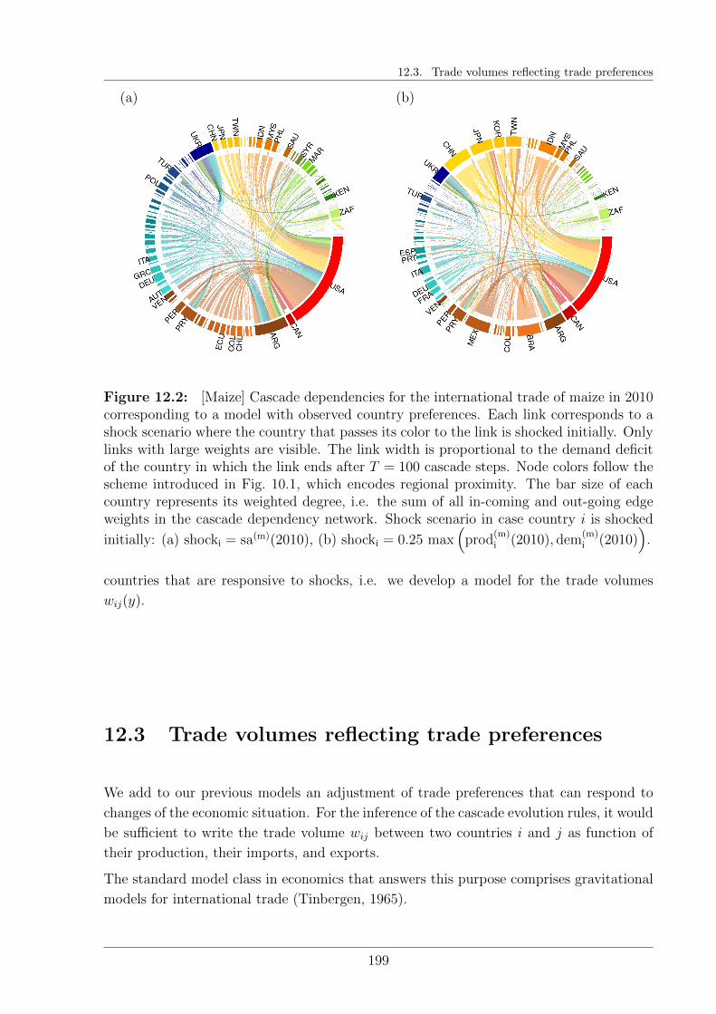
12.3. Trade volumes reflecting trade preferences
(a) (b)
Figure 12.2: [Maize] Cascade dependencies for the international trade of maize in 2010corresponding to a model with observed country preferences. Each link corresponds to ashock scenario where the country that passes its color to the link is shocked initially. Onlylinks with large weights are visible. The link width is proportional to the demand deficitof the country in which the link ends after T = 100 cascade steps. Node colors follow thescheme introduced in Fig. 10.1, which encodes regional proximity. The bar size of eachcountry represents its weighted degree, i.e. the sum of all in-coming and out-going edgeweights in the cascade dependency network. Shock scenario in case country i is shocked
initially: (a) shocki = sa(m)(2010), (b) shocki = 0.25 max(
prod(m)i (2010), dem
(m)i (2010)
).
countries that are responsive to shocks, i.e. we develop a model for the trade volumes
wij(y).
12.3 Trade volumes reflecting trade preferences
We add to our previous models an adjustment of trade preferences that can respond to
changes of the economic situation. For the inference of the cascade evolution rules, it would
be sufficient to write the trade volume wij between two countries i and j as function of
their production, their imports, and exports.
The standard model class in economics that answers this purpose comprises gravitational
models for international trade (Tinbergen, 1965).
199
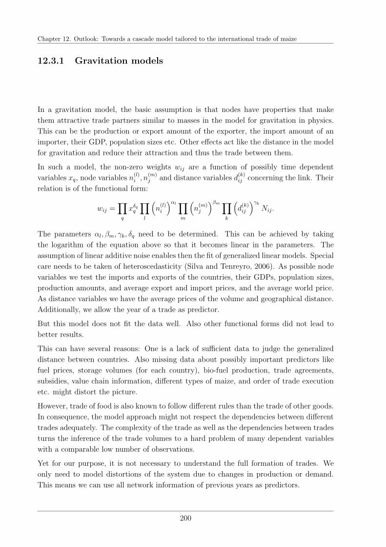
Chapter 12. Outlook: Towards a cascade model tailored to the international trade of maize
12.3.1 Gravitation models
In a gravitation model, the basic assumption is that nodes have properties that make
them attractive trade partners similar to masses in the model for gravitation in physics.
This can be the production or export amount of the exporter, the import amount of an
importer, their GDP, population sizes etc. Other effects act like the distance in the model
for gravitation and reduce their attraction and thus the trade between them.
In such a model, the non-zero weights wij are a function of possibly time dependent
variables xq, node variables n(l)i , n
(m)j and distance variables d
(k)ij concerning the link. Their
relation is of the functional form:
wij =∏q
xδqq∏l
(n
(l)i
)αl∏m
(n
(m)j
)βm∏k
(d
(k)ij
)γkNij.
The parameters αl, βm, γk, δq need to be determined. This can be achieved by taking
the logarithm of the equation above so that it becomes linear in the parameters. The
assumption of linear additive noise enables then the fit of generalized linear models. Special
care needs to be taken of heteroscedasticity (Silva and Tenreyro, 2006). As possible node
variables we test the imports and exports of the countries, their GDPs, population sizes,
production amounts, and average export and import prices, and the average world price.
As distance variables we have the average prices of the volume and geographical distance.
Additionally, we allow the year of a trade as predictor.
But this model does not fit the data well. Also other functional forms did not lead to
better results.
This can have several reasons: One is a lack of sufficient data to judge the generalized
distance between countries. Also missing data about possibly important predictors like
fuel prices, storage volumes (for each country), bio-fuel production, trade agreements,
subsidies, value chain information, different types of maize, and order of trade execution
etc. might distort the picture.
However, trade of food is also known to follow different rules than the trade of other goods.
In consequence, the model approach might not respect the dependencies between different
trades adequately. The complexity of the trade as well as the dependencies between trades
turns the inference of the trade volumes to a hard problem of many dependent variables
with a comparable low number of observations.
Yet for our purpose, it is not necessary to understand the full formation of trades. We
only need to model distortions of the system due to changes in production or demand.
This means we can use all network information of previous years as predictors.
200
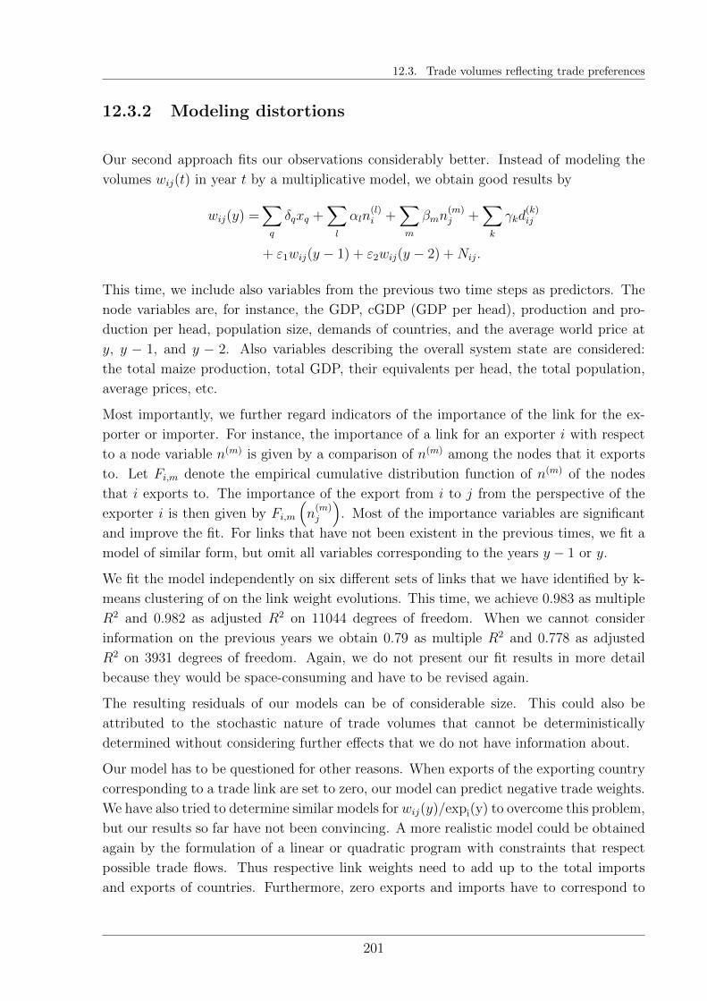
12.3. Trade volumes reflecting trade preferences
12.3.2 Modeling distortions
Our second approach fits our observations considerably better. Instead of modeling the
volumes wij(t) in year t by a multiplicative model, we obtain good results by
wij(y) =∑q
δqxq +∑l
αln(l)i +
∑m
βmn(m)j +
∑k
γkd(k)ij
+ ε1wij(y − 1) + ε2wij(y − 2) +Nij.
This time, we include also variables from the previous two time steps as predictors. The
node variables are, for instance, the GDP, cGDP (GDP per head), production and pro-
duction per head, population size, demands of countries, and the average world price at
y, y − 1, and y − 2. Also variables describing the overall system state are considered:
the total maize production, total GDP, their equivalents per head, the total population,
average prices, etc.
Most importantly, we further regard indicators of the importance of the link for the ex-
porter or importer. For instance, the importance of a link for an exporter i with respect
to a node variable n(m) is given by a comparison of n(m) among the nodes that it exports
to. Let Fi,m denote the empirical cumulative distribution function of n(m) of the nodes
that i exports to. The importance of the export from i to j from the perspective of the
exporter i is then given by Fi,m
(n
(m)j
). Most of the importance variables are significant
and improve the fit. For links that have not been existent in the previous times, we fit a
model of similar form, but omit all variables corresponding to the years y − 1 or y.
We fit the model independently on six different sets of links that we have identified by k-
means clustering of on the link weight evolutions. This time, we achieve 0.983 as multiple
R2 and 0.982 as adjusted R2 on 11044 degrees of freedom. When we cannot consider
information on the previous years we obtain 0.79 as multiple R2 and 0.778 as adjusted
R2 on 3931 degrees of freedom. Again, we do not present our fit results in more detail
because they would be space-consuming and have to be revised again.
The resulting residuals of our models can be of considerable size. This could also be
attributed to the stochastic nature of trade volumes that cannot be deterministically
determined without considering further effects that we do not have information about.
Our model has to be questioned for other reasons. When exports of the exporting country
corresponding to a trade link are set to zero, our model can predict negative trade weights.
We have also tried to determine similar models for wij(y)/expi(y) to overcome this problem,
but our results so far have not been convincing. A more realistic model could be obtained
again by the formulation of a linear or quadratic program with constraints that respect
possible trade flows. Thus respective link weights need to add up to the total imports
and exports of countries. Furthermore, zero exports and imports have to correspond to
201

Chapter 12. Outlook: Towards a cascade model tailored to the international trade of maize
non-existent trade volumes. This makes a multiplicative model a more realistic ansatz.
We still employ the model that we have introduced to obtain preliminary results. How-
ever, we assume that the trade preferences of countries are only proportional to predicted
reasonable values. To be precise, we assume
epij(t) =max (wij(y), 0)
expi(y, t), ipij(t) =
max (wij(y), 0)
impj(y, t)
as value a link (i, j) for an exporter, denoted by epij, of for an importer, denoted by ipij.
The dependence on y and t shall indicate that the variables correspond to variables that
can change according to our trade reorganization model. wij(y) corresponds to the weights
that we have obtained by our introduced model that acknowledges a changed economic
situation because of a shock. expi(y, 0) and impj(y, 0) are defined by respective sums of
these weights. In later cascade times t, expi(y, t) and impj(y, t) correspond only to sums
of weights which match partially the trade preferences of the involved trade partners.
Because of the drawbacks that we have discussed, the weights cannot become realized
completely. Neither can the exports and demands that we have estimated independently
from the weights.
We therefore interpret the inappropriate model as preferred trade outcomes of countries,
if these are realizable. A simple matching of these preferences is discussed next.
Cascade dynamics
There are several meaningful ways to define a cascade process based on given demand,
export, and weight informations. Again, we could start from an observed trade structure
and distort it according to preferences of shocked countries and possible trade counterparts.
As neither our demand and export preferences nor our trade volume preferences change
in the course of a cascade, we have decided to not mix structures and preferences. We
therefore employ a simple matching of new preferences similar to our previous model.
For each link weight, trades are established by the maximal amount that both countries
agree on according to their export and import preferences. In a next step, they revise their
valuation of each trade considering only remaining possible trade matches of the previous
time step. This ensures that the order of country consideration in one time step cannot
influence our results. Successively, we built a trade network respecting the estimated trade
preferences as far as reasonable.
Our model cannot really be interpreted as distortion of observed structures to construct
an alternative trade network. This could instead be realized by a different reading of our
model fits. Here, we assume that the demand of a country expresses its desire of a good
considering its price etc. Furthermore, we could see it as quantity that changes in the
202
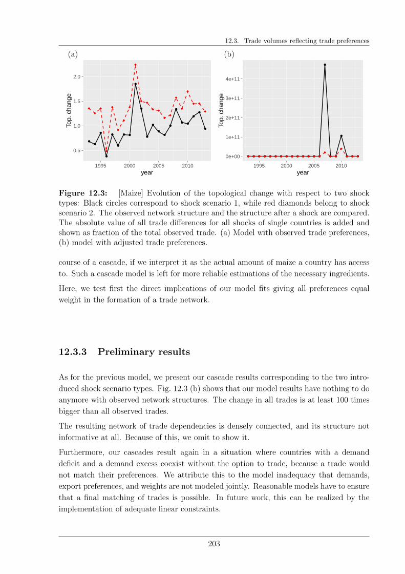
12.3. Trade volumes reflecting trade preferences
0.5
1.0
1.5
2.0
1995 2000 2005 2010year
Top.
cha
nge
0e+00
1e+11
2e+11
3e+11
4e+11
1995 2000 2005 2010year
Top.
cha
nge
(a) (b)
Figure 12.3: [Maize] Evolution of the topological change with respect to two shocktypes: Black circles correspond to shock scenario 1, while red diamonds belong to shockscenario 2. The observed network structure and the structure after a shock are compared.The absolute value of all trade differences for all shocks of single countries is added andshown as fraction of the total observed trade. (a) Model with observed trade preferences,(b) model with adjusted trade preferences.
course of a cascade, if we interpret it as the actual amount of maize a country has access
to. Such a cascade model is left for more reliable estimations of the necessary ingredients.
Here, we test first the direct implications of our model fits giving all preferences equal
weight in the formation of a trade network.
12.3.3 Preliminary results
As for the previous model, we present our cascade results corresponding to the two intro-
duced shock scenario types. Fig. 12.3 (b) shows that our model results have nothing to do
anymore with observed network structures. The change in all trades is at least 100 times
bigger than all observed trades.
The resulting network of trade dependencies is densely connected, and its structure not
informative at all. Because of this, we omit to show it.
Furthermore, our cascades result again in a situation where countries with a demand
deficit and a demand excess coexist without the option to trade, because a trade would
not match their preferences. We attribute this to the model inadequacy that demands,
export preferences, and weights are not modeled jointly. Reasonable models have to ensure
that a final matching of trades is possible. In future work, this can be realized by the
implementation of adequate linear constraints.
203
Chapter 12. Outlook: Towards a cascade model tailored to the international trade of maize
12.4 Summary and outline of possible model improve-
ments
In summary, the goal is to estimate the response of a food trade network to a shock.
This shock can originate from a production decrease or demand increase (e.g. caused by
population growth) in specific countries of the world. Its size and location is an assumption
in a stress test scenario. Thus, it is an exogenous variable in our model. The trade volumes
between each pair of countries are our final response variables.
Besides limited data quality and missing information about possible predictors, the main
statistical challenge is the high number of dependent variables given a relatively small
number of observations.
We address this challenge by modeling distortions by a simplification of the goal. Instead of
asking: “How is the trade network formed each year and what determines its evolution?”,
we ask the simpler question: “How does it respond to small changes in the production and
demand of specific countries?”. Thus, we only need to distort the original network that
is given by data. This network has been formed by complicated but realistic processes
beyond our control. But we capture them indirectly and preserve the original dependence
between the variables to a large extend.
The predictive quality of this approach is limited to relatively small shock sizes, small
distortions and small time windows. For bigger shocks, the observed processes might
change their nature and, on the long run, other variables beside production and demand
might change and influence the evolution of the trade network. Only a deeper process
understanding could solve this issue. But, with the data at hand, this is not feasible on
the level of trade volumes between countries.
These considerations form the maxim of our modeling approach: We try to introduce as
little distortion as possible to observed structures. Consequently, we model distortions as
a cascade process that introduces changes to a network by relatively small successive local
adjustments.
Our previously analyzed model of cascading export restrictions is limited in its scope,
as it does not consider the following relevant aspects: (1) Countries cannot only reduce
exports, they can also increase their imports. (2) Prices or other global variables influence
trade decisions and can even introduce systemic feedback. (3) Countries value their trade
relationships differently under changing economic conditions. (4) The trade networks of
the different considered staples are highly coupled. This calls for multiplex perspective.
Furthermore, it does not acknowledge the high uncertainty in a country’s trade decisions.
Many factors can determine different crises response, for instance, human decisions. Most
of these factors cannot be modeled deterministically.
204

12.4. Summary and outline of possible model improvements
We have presented preliminary approaches to address issues (1)-(3) for the international
trade of maize.
As we have shown, our models are still inadequate, as they do not respect natural con-
straints that trade flows have to fulfill. As these constraints are linear, this issue can
be solved by the formulation of a quadratic program that serves the joined estimation of
parameters in models for changing demands, exports and trade volumes. To employ a mul-
tiplex view, the quadratic program could be complemented to consider further variables
corresponding to other staples.
On the basis of the obtained models, a cascade process can be defined that successively
changes the exports and imports of nations. These updated variables could again serve as
input in a new estimation of affected weights.
Further possible steps in a thorough systemic risk analysis of international staple food trade
are discussed in the next chapter, when we outline possible future research directions.
In summary, the goal is to estimate the response of the network representing the inter-
national trade of maize to a shock. This shock can originate from a production decrease
or demand increase (e.g. caused by population growth) in specific countries of the world.
Its size and location is an assumption in a stress test scenario. Thus, it is an exogenous
variable in our model. The trade volumes between each pair of countries are our response
variables.
Besides limited data quality and missing information about possible predictors, the main
statistical challenge is the high number of dependent variables given a relatively small
number of observations. The data quality issue is addressed in the end by comparing dif-
ferent reasonable scenarios to get an idea how sensitive our approach is to data distortions
and our model assumptions.
The second statistical challenge is approached by a simplification of the goal. Instead of
asking: ”How is the trade network formed each year and what determines its evolution?”,
we ask the simpler question: ”How does it respond to small changes in the production and
demand of specific countries?”. Thus, we only need to distort the original network that
is given by data. This network has been formed by complicated but realistic processes
beyond our control. But we capture them indirectly and preserve the original dependence
between the variables to a large extend.
The predictive quality of this approach is certainly limited to relatively small shock sizes,
small distortions and small time windows. For bigger shocks, the observed processes might
change their nature and, on the long run, other variables beside production and demand
might change and influence the evolution of the trade network. Only a deeper process
understanding could solve this issue. But, with the data at hand, this is not feasible on
the level of trade volumes between countries. Still, our general approach allows a trade
dependence analysis that incorporates cascade effects.
205

Chapter 13
Summary and conclusions
13.1 Contributions
In this thesis, we have deepened the understanding of cascade processes following a generic
modeling approach. This way, we have investigated one of the main sources of systemic
risk and identified ample factors that constitute it.
We understand systemic risk as emergent property of a system that is comprised of many
interacting agents, which are modeled by nodes in a network. Their interaction is charac-
terized by the local load distribution of a failing node and lets us distinguish three different
cascade model classes: the Constant Load (CL), the Load Redistribution (LRD), and the
Overload Redistribution (OLRD) class.
They share some common overarching principles, which are of focus in Part I of this thesis.
Also their differences, especially in relation to the role of hubs and leaves in the course
of a cascade, are discussed in detail. Our main contribution beyond the comparison of
different models and possible ways to reduce systemic risk is of methodological nature.
We thus summarize our main contributions in this respect. Afterwards we discuss in more
detail our findings and insights that have been enabled by our methodological advance-
ments.
13.1.1 Methodological contributions
Part I. We have derived a local tree approximation (LTA), also known as branching pro-
cess approximation, for the cascade size evolution in infinitely large configuration model
type random graphs. This analytical result is in perfect correspondence with simulation
results. Furthermore, we have gained the insight that all cascade time steps are cor-
rectly computed. This is valid for all degree distributions with finite second moment and
207
Chapter 13. Summary and conclusions
arbitrary threshold distributions.
We have extended the class of constant load models that can be tackled by this approach.
In the here provided form, it comprises also models where the distributed load can depend
on properties of the failing node. Furthermore, several load redistribution and overload
redistribution models can be covered by our derivations, including the LRD and OLRD
LLSS variant. To our knowledge, this has not been possible before.
Employing a different perspective than the common generating function approach has
paved the way for these results. We describe the load that a failed neighbor distributes
by a random variable whose distribution is calculated iteratively. The heterogeneity of
loads originates in a concept that we have introduced as damage diversification. As we
found, this concept is core to the understanding of the role of hubs in a cascade, especially
for LRD and OLRD models. Furthermore, it points to an additional option to reduce
systemic risk.
Part II. We have extended our analytic local tree approximation (LTA) to a multiplex
setting, in which we introduce a new type of link, a semi-dependency link. Interestingly, we
find that the coupling between the layers can mainly be achieved by adapting the response
function.
Similarly, we also have integrated systemic feedback in our iteration procedure.
As a third contribution of Part III, we have moved our focus to the study of finite networks.
Our derivations of the full cascade size distribution in finite fully connected and star-shaped
networks rely solely on combinatorial arguments and the high symmetry of the considered
networks. From a methodological perspective, these derivations differ completely from the
earlier results. They apply to a relatively general class of cascade processes and are valid
for arbitrary threshold distributions.
Part III. Because of the unsymmetrical finite network structure that is defined by the
data on international trade of staple food, we cannot describe the cascade risk by analytic
means. Instead, we have employed Monte-Carlo simulations to study systemic risk. The
transfer and adaptation of cascade models to describe the evolution of the international
trade of staples, as presented in this thesis, is a methodological advancement in food trade
research. Furthermore, we have defined a set of new systemic risk indicators that measure
different aspects of the cascade evolution. These could be used in an assessment of the
shock resilience of international staple trade.
208
13.1. Contributions
13.1.2 Main insights
Modeling systemic risk under network uncertainty
In Part I, we have focused on average properties to measure cascade effects on undirected
random graph ensembles defined by prescribed degree and threshold distributions. Two
influences on the amplification of failures can be investigated in this setting: the hetero-
geneity in the diversification behavior of nodes and heterogeneity in their robustnesses.
From a modeling perspective, random graph ensembles reflect network uncertainty, i.e.
missing information about a given, fixed network structure or quickly changing network
topologies.
In our studies, we have extended the analysis of the three cascade model classes identified
by Lorenz et al. (2009). However, investigations presented by Lorenz et al. (2009) were
limited to fully connected, and partially regular, topologies. Because of this simplifica-
tion, the different exemplary models in each class were indistinguishable in their cascade
dynamics. In this thesis, we introduce heterogeneous degrees to the study of these model
classes. With this extension, we were able to reveal differences between the exemplary
models for all three classes.
Considering the phase diagrams with respect to the studied threshold parameters, we
observe sudden regime shifts for Constant Load (CL) and Load Redistribution (LRD)
models, and in principle low systemic risk for Overload Redistribution (OLRD) models.
This is similar to the results presented in Lorenz et al. (2009). However, the impact of the
overall connectivity, the role of hubs and leaves in the course of a cascade, and consequently
their endowment with different thresholds, vary widely among the models. Especially
correlations between threshold and degree distributions lead to strong deformations of the
observed phase diagrams.
The trade-off between cascade exposure and damage diversification. Common
to all cascade processes on undirected networks is that failures of nodes with high degrees
have the potential to cause many subsequent failures. Thus, in a systemic risk reduction
scheme, their failure probabilities usually need to be reduced or their failures mitigated.
A failure mitigation effect is present in most of our studied models, except the Constant
Load Exposure Diversification model (CL ED). Usually, the damage that a failing node
inflicts is shared between its functional network neighbors. Consequently, if the count of
neighbors is higher, each of them receives a smaller amount of load. At the same time,
hubs face a high failure risk because each additional link introduces a possible way to
receive additional load in case of a neighbor’s failure. Still, the existence of hubs can be
advantageous for a system. On the one hand they provide connectivity in times of ”normal”
system operation. On the other hand, if they fail in the course of a cascade, their failure
cuts many cascade paths and has hence the potential to decrease the total cascade size.
209
Chapter 13. Summary and conclusions
This effect is particularly prominent in Constant Load Damage Diversification (CL DD)
models, where the damage that a node failure inflicts is constant over time.
Time of failure. However, in Load Redistribution (LRD) and Overload Redistribution
(OLRD) models, nodes accumulate load over time and distribute it (at least partially)
further in case of their failure. If they distribute a high amount of load, their failure causes
many subsequent failures with a high probability. As in these models nodes accumulate
load over the course of a cascade, their early failures can be beneficial for mitigating large
cascades.
Because of the accumulation of load in these models, we have observed much higher
systemic risk for the Local Load Sharing with load Conservation (LLSC) model than for
the Local Load Sharing with load Shedding (LLSS) variant in case of Load Redistribution
(LRD). In case of the former, the network interconnectivity increases over time, since
neighbors of failing nodes become connected. Thus, also the degrees of nodes increase and
the cascade process develops similarly as on a fully connected topology. In contrast, Local
Load Sharing with Load Conservation (LLSC) incorporates less systemic risk in case of
the Overload Redistribution models. Here, only small amounts of overload are distributed,
such that a high connectivity, i.e. good damage diversification, provides protection for the
neighborhood of failing nodes with a high degree.
In general, the time of a node’s failure is determined by its threshold. Consequently,
different threshold allocation schemes can influence who fails earlier: hubs or leaves.
The interplay between system robustness and topology. Although system perfor-
mance is not explicitly modeled, we have assumed that it is implicitly reflected in the given
degree and threshold distributions. In case that the overall system performance depends
only on these two distributions and not on the microscopic structure of a network or the
combination of threshold and degree of single nodes, a reallocation of thresholds would not
change the overall system performance. However, such a reallocation can have substantial
impact on systemic risk. Here, we have studied three different reallocation schemes.
Random failures (rf) have served as our benchmark scheme, since a random allocation of
thresholds, independent of a node’s degree, is the simplest and most reasonable1 assump-
tion. Furthermore, hubs and leaves have no a-priori different failure risk. In contrast,
the central failures (cf) scheme leads to the early failure of hubs, as nodes with a higher
degree receive smaller thresholds. The reverse image we have studied by considering the
peripheral failures (pf) scheme, where hubs receive higher thresholds than leaves.
One of the two extreme scenarios, peripheral failures (pf) or central failures (cf), usually
leads to a reduction of systemic risk, while the other supports a further amplification of
failures. We find a general tendency that for model variants which expose the system to
1This choice maximizes the entropy, if no information about the correlation between threshold anddegree distribution is available.
210

13.1. Contributions
lower systemic risk than other models in the same class, central failures lead to smaller
cascades. And vice versa, peripheral failures (pf) are better suited to reduce the cascade
risk originating in models that show higher cascade risk for random failures (rf).
Our explanation for this observation is that models showing lower systemic risk in case of
random failures usually do so because of a beneficial damage diversification effect. Central
failures (cf) support this effect even further and lead to an early failure of hubs. In
contrast, peripheral failures (pf) prevent the failure of hubs. This hinders the amplification
of cascades if the failure of hubs are the most problematic events.
However, in direct comparison, the best combinations of cascade model variant and thresh-
old allocation, for instance, CL ED pf and DD cf, show no consistently better results than
the others. Usually, one combination reduces the cascade risk in regions of high systemic
risk, while the other one exposes the system to lower risk for most other parameters. This
poses a system design question, which we have discussed in detail in Chapter 4. The
answer depends on the preferences and risk aversion of the respective stakeholders.
Extensions and limitations of modeling assumptions
We have challenged the modeling assumptions used in Part I by three different extensions
of our previous model setting.
Multiplex. Modeling a complex system as network usually means a significant simpli-
fication of the structure. Different components are associated with similar nodes, while
their various interactions are subsumed in one type of link.
We have therefore extended our model complexity by an additional second network layer,
coupled to the original one. Furthermore, we have introduced another type of link, a
semi-dependency link, characterizing this coupling. Via this link, cascades can propagate
in an asymmetric way. While a failure in the main layer leads to the immediate failure of
the corresponding node in the second layer, the other way around, only the threshold in
the original layer is reduced.
This setup is motivated by an example, where firms face the decision to split their business
in a core and subsidiary business. This scenario is best represented by the constant load
exposure diversification model. Clearly, both strategies, leaving the networks as it is, as
well as the split into subsidiary businesses, lead to a certain exposure to cascades. We
quantify this exposure by an analytic LTA of the average final cascade size.
Which decision incorporates the lower systemic risk crucially depends on the coupling
strength of the two layers. For lower coupling, a split of businesses is advantageous, if
the core layer is relatively robust. Interestingly though, we observe a sudden regime shift
for increasing coupling strength. At a certain point, cascades lead to an almost complete
system break-down via a feedback mechanism between both layers. We provide an estimate
211
Chapter 13. Summary and conclusions
for this critical point.
As the phase diagrams, which we observe, differ qualitatively significantly from our results
on single layers, we conclude that the multiplex nature of a system definitely needs to be
regarded in a realistic systemic risk model.
Systemic Feedback. Previously, we have assumed that load is only distributed locally to
functional network neighbors. However, often global information about the system state
is available and nodes respond accordingly. We have studied an exemplary Constant Load
Exposure Diversification model in which the downward trend in the course of a cascade
is reinforced. Interestingly, this set-up leads to extremely similar results as a Load Re-
distribution model on a fully connected network structure. In fact, the systemic feedback
mechanism that we have investigated could equivalently be interpreted as additional global
distribution of load.
From this and other findings presented in this thesis, we see that the model class boundaries
are often not sharply defined. The above example even pinpoints to a possible interpolation
between the CL and the LRD class. We conclude that macro state observations are
obviously not sufficient to deduce dynamics on the micro level.
Finite networks. In the previous chapters, we have studied the average cascade size
in infinitely large random graph ensembles. However, real world systems are usually
finite and the cascade outcomes are variable. We have derived a closed form solution for
the probability distribution of the final cascade size for fully connected and star-shaped
networks of arbitrary finite size N . With our approach, CL as well as LRD models can
be captured. However, models of OLRD type introduce an additional challenge that we
cannot solve yet.
Remarkably, despite the high symmetry of the considered network topologies and the
threshold distributions, we find asymmetric and broad cascade size distributions for several
parameters. Even for fully connected networks consisting of N = 107 nodes, we still find
bi-modular shapes. We conclude that in this setting, the average is a bad measure of
cascade size, as it is only a poor representation of the actual systemic risk. This finding
is of special interest, as it is common practice to report only the average cascade risk in
empirical studies.
Interestingly, these results question our conclusions from the previous chapters to some
extent. Before, the CL Exposure Diversification (ED) seemed to outperform other con-
stant load models on average when nodes with a higher degree receive higher thresholds
(pf). Yet, in the presence of hubs, as in star-shaped networks, we find a tendency to-
wards bi-modular cascade size distribution for the ED model. In contrast, the Damage
Diversification (DD) variant leads more reliably to small systemic risk.
We conclude that a thorough systemic risk analysis needs to incorporate the shape of the
full cascade size distribution instead of focusing on one-dimensional summary measures,
212
13.1. Contributions
as for instance, the average.
Modeling systemic risk in a data driven approach
Ultimately, we study models, like the ones introduced in this thesis, for the purpose to
better understand real-world systems. Specifically, we study the international trade of
staple foods.
The final goal is to describe the reorganization of the international trade of staples as
response to changing productions and demands. We have approached this goal by first
steps towards cascade model improvements that regard our insights from the previous
chapters. Unfortunately, we cannot transfer our findings par for par, as we have adjusted
the model dynamics to fit our purpose. However, we have developed an intuition which
general aspects are worth a consideration.
In our study of this particular real-world system, we have first identified the hubs and leaves
and the basic properties of the topological structure. Moreover, we have investigated the
allocation of thresholds. As we have additional information about the yearly time evolution
of the networks, we have also observed trends in the network changes.
Descriptive data analysis. We have analyzed and compared the yearly evolution of
four coupled international trade networks regarding the four major internationally traded
staples: maize, rice, soy, and wheat.
All these networks show increasing interconnectivity. This can be partially explained by
a growing production and for maize, rice, and soy even a growing production per head.
However, the share of traded goods versus the total production still increases for all staples
except maize. Especially, soy is traded to a large extend: 34 % of the whole production
in 2013.
This trade is facilitated by a growing number of trade links between countries. However,
we observe that the distribution of weights, i.e. trade volumes, is right skewed. Thus, a
significant share of all trade is constituted by a relatively small number of links. The weight
heterogeneity is highest for soy and still seems to be further increasing. Interestingly, wheat
is traded much more equally, as can be observed by low link weight heterogeneity.
There are further differences in the stability of these big trade volumes over time. Re-
markably, we find a structural change in 2013 for several staples. Most interestingly, the
biggest trade volumes shifted. For instance, the maize exports from the USA to Japan
declined, which in turn is partially compensated by exports from Brazil to Japan. We
hypothesize that this decline can be mainly attributed to an increase in demand of the
USA.
However, the possible causal explanations are manifold. We test the implications of several
assumptions in the models we have developed in Chapter 11 and Chapter 12. These
213
Chapter 13. Summary and conclusions
models attribute a topological change to a distortion of the production or the demand
distributions. We also present a more advanced model, in which demands depend also on
the production distribution at least indirectly via prices.
Cascading export restrictions. As a first approach to better understand the reorga-
nization of the trade networks as response to local shocks, we have investigated a simple
model for cascading export restrictions. This model originates in the studied Overload
Redistribution models, but has been adapted in several ways to match our application
better. Given the results of this model, in a second step we have constructed a directed
weighted network in which each link corresponds to the outcome of a shock scenario. The
resulting network can be interpreted as a higher order representation of trade dependen-
cies, while only the first order is given by the original trade network. We argue that
such a cascade dependency network gives valuable insights about more realistic economic
dependencies than direct trade relationships, as it also acknowledges the capabilities of
countries to mitigate shocks. This representation furthermore addresses the issue of in-
formation loss introduced by systemic risk summary measures, as it provides an overview
about the heterogeneity of cascade outcomes.
In contrast to the analysis presented in the previous chapters, temporal information is
provided as well. Because of this, we have been able to investigate the evolution of the
final fraction of failed nodes for years 1992 to 2013. We have complemented the earlier
presented static measures by several systemic risk indicators that capture different aspects
of the evolving cascade.
We have found that the number of countries, that are affected by cascades, increased in
the considered time period. This can be mainly attributed to the growing trade inter-
connectivity. As result, at the end of the observation period shocks are shared by a high
number of countries in relatively equal proportions. Also, the fraction of the population
that would be affected by the shock scenarios we have considered is rather small. We
have interpreted this as a sign of good risk diversification. Our findings are also robust
with respect to our empirical observations of structural changes of the largest trades in
2012/2013.
Let us note that these conclusions do not take into account the vulnerability of the system
to trade deprivations. Indeed, trade distortions usually come along with a loss of the
benefits associated with canceled trades.
We have found that the reorganization of the networks due to trade restrictions is con-
siderable. Often, cascades evolve over long times and comprise a high number of export
withdrawals. Except for soy trade, the fraction of trade that is possibly canceled increases
over time. This diminishing trade has especially negative consequences for trade interme-
diaries. Our model has proven useful in the identification of such trade intermediaries.
These are characterized by by a high cascade betweenness centrality, which measures a
214
13.2. Future research
node’s vunlerability to trade losses.
Adding model complexity. Several assumptions in our cascading export restrictions
model are critical in a realistic risk scenario. The following aspects need to be revised in
next steps: 1) Import increases are not possible in the mitigation of shocks. 2) Countries
cannot respond to the measurements of the system state. Prices or the overall production
amount do not influence trade decisions. 3) Preferences of countries concerning their
trade partners are not reflected adequately. Some links might break down completely,
while others are strengthened in response to shocks. 4) Food trade networks are studied
separately. In reality, strong couplings between the networks are observed, as consumers
can substitute one staple by another in response to price increases. 5) Price elasticities
are not considered. However, people adjust their demand accordingly.
We have given an outline, how these challenges can be addressed and have discussed first
steps towards the considered model improvements.
13.2 Future research
Modeling Framework. We see ample of opportunities to continue our research in the
setting of random graph ensembles. On the basis of our methodological contribution, we
could explore how the cascade outcome depends on other threshold distributions or on
the average of the degree distribution. We could ask whether the existence of a cascade
window, as encountered by Gleeson and Cahalane (2007) for the Constant Load Exposure
Diversification model, is in fact a relatively general property of cascade processes. Further-
more, we could study the impact of the relation between the fraction of hubs and leaves on
systemic risk. Thus, we would optimize the degree distribution under some constraints,
for instance a fixed average degree.
A challenge that we might be able to solve in future is to provide an analytic description of
the average cascade size corresponding to the Local Load Sharing with load Conservation
(LLSC) models, i.e. a fiber bundle model with local load sharing. A combination of
our branching process approximation for the Local Load Sharing with load Shedding
(LLSS) variant and advancements for cascading processes in clique based random graphs
by Hackett and Gleeson (2013) seems to be a promising first step.
In the first two parts of this thesis, we have measured systemic risk by the (average)
fraction of failed nodes. This does not penalize for a loss of connectivity. Conversely, we
have regarded early disconnections to be positive, if they cut possible path ways that a
cascade process can take. However, the functionality of real world systems depends often
critically on the connectedness of its components. Consequently, we would ask in future
for the size distribution of its connected components. Similarly, we could measure system
performance explicitly in different ways and study its evolution in the course of a cascade.
215
Chapter 13. Summary and conclusions
Furthermore, we could introduce additional model complexity while preserving analytic
tractability. For instance, interventions that increase the robustness of specific nodes or
possible recoveries of failed nodes with time delay are often studied in the context of
cascade processes and considered as practically relevant.
In principle, we could also analyze cascade processes where the load distribution mecha-
nisms of our classes are mixed or study multiplexes with layers corresponding to different
load distribution mechanisms. However, we would object arbitrary extensions of the pre-
sented generic models, especially because the number of options seems to be infinite.
Instead, we would focus on extensions which have or could have an equivalent in an
application setting. We would be guided by three questions: 1) How does systemic risk
emerge? 2) How do specific topological network or process features impact the evolution
of cascades? 3) How can systemic risk be reduced?
In an economic networks setting, answers to the above questions could be based on agent
based models in which nodes maximize, for instance, individual utility functions. On this
basis they could make decisions about their allocation of resources. This research direction
would especially be interesting, as it studies the implications of a systemic perspective,
where the system safety is not necessarily aligned with the interests of individual nodes.
This would suggest to test several incentive schemes to reduce systemic risk to compensate
for the utility loss that specific nodes would encounter in this situation. In the context of
financial networks, several measures are considered that organize the system with a macro
viewpoint, for instance, taxation of systemic risk increasing trades or the introduction of
a central counter party.
Multiplex. Ample extension options exist for studies of cascade processes on multiplexes.
We only focus on possible immediate next steps based on our investigations.
First and foremost, from an analytic point of view, it would be straight forward to intro-
duce semi-dependency links between a number of network layers where nodes according
to other load distribution mechanisms. Furthermore, we could also handle heterogeneous
coupling strengths and allow that only a fraction q of all nodes could be coupled to nodes
in another layer. We would expect that we could also observe a sudden regime shift when
varying q. Additionally, a higher number of interlayer links starting from single nodes are
a possibility.
Especially interesting for the application that has motivated our model, we could allow a
mixture of business splits and business merges. Moreover, it would be more realistic to
consider that certain properties of nodes in one layer preferably attract nodes with certain
properties in another layer. As example, nodes with high degrees in one layer have a higher
chance to connect to nodes that also have a high degree in the other layer to increase risk
diversification in both layers.
Furthermore, we have not studied different threshold allocation schemes in the multiplex
216
13.2. Future research
setting yet. Also, the threshold of a node could imply a preference for establishing links
to nodes with a similar threshold, or to nodes with a higher threshold to acquire more
capital.
In summary, we could improve our model in such a way that it reflects several strategies
of firms concerning their merging and business split decisions.
Finite networks and volatility. As we have found, a thorough systemic risk analysis
in finite systems needs to consider the full final cascade size probability distribution. This
insight will influence all of our future work. Furthermore it has sparked a new research
question: What are the main reasons for high uncertainty, i.e. rather broad distributions,
in the cascade outcome? Moreover, is there a point in time at which we can narrow down
the cascade outcome with higher certainty?
As extension of our framework models we could also consider stochastic cascade dynamics
as developed by Lorenz et al. (2009) and estimate the implications of this additional
stochastic element. How does this increase the uncertainty of the cascade outcome?
We would start in each case from a network motif based analysis and look for similar
patterns. Additionally, we would be interested in the question how our findings correspond
to adjacency matrix properties of the considered network structure and, of course, on
properties of a given threshold distribution.
For this analysis, but also in practice, it might be valuable to have risk measures at
hand to summarize relevant properties of the cascade size distribution. Although such
a summary might be inadequate in all possible cases, it would be worthwhile to identify
certain classes of processes or sets of parameters, where such measures carry meaningful
information. These measures would need to reflect criteria that we relate with low systemic
risk. This would allow us to look for topological improvements that reduce systemic risk in
this sense. For instance, starting from a given network structure we could redirect certain
links in a Greedy fashion.
Resilience of international food trade networks. This research direction we find
especially promising to continue with, as it relates to one of the millennium development
goals, the guarantee of world wide food security.
There are a multitude of problems that could and need to be worked on. For instance,
only the modeling of possible shocks to the production system is a demanding task tackled
by the joined effort of many researchers. Also the identification of the stakeholders in the
world food system and their interests or strategies that could enter an agent based model
are a challenge, which is often addressed in case studies.
Our complex systems approach requires strong simplifications of these tasks on the macro
level, but has to capture at the same the most important aspects. We rely on deepening
the understanding of the mentioned issues. Our models have to be successively improved
217

Chapter 13. Summary and conclusions
to capture as many realistic aspects as possible. Moreover, we can investigate further how
international trade is constituted and find ways to control for effects like changing trade
agreements, subsidies, import taxation etc.
Another issue is, that we make strong causal assumptions about the propagation of cas-
cades and the value of trade relationships for the involved countries. These call for a
rigorous statistical validation. First, we have to focus on our model selection. In a next
step, we would formulate and implement a linear program (LP) to fit an adequate model
for the link weights. It has to respect that the link weights have to fulfill constraints so
that the import and export of countries are correctly matched. Furthermore, we need to
take care of over-fitting also in our models for country strategies, for instance by cross-
validation. Theoretically, the resulting model parameters are stochastic and introduce
variability in our cascade outcomes. This variability needs to be reported as well. More-
over, it helps us judge the quality of our model. For instance, we could try to explain
the trade network evolution with our model by comparing our model results with given
data. Thus we would measure the change in our predictors, i.e the production amount,
population, gdp of countries, etc., and use these as model input and describe the change
of the international staple trade networks by a cascade process. This would be bases on a
multiplex view that we have to employ further and incorporate substitution possibilities
of different types of crops. Additionally, we would seek to explain also the creation or
existence as well as deletion of links and not only the trade volume along existing links.
Moreover, it might be possible to infer to some degree the usage of quantities traded
along certain links with the help of the usage data in countries. This would allow us to
develop more realistic shock scenarios and risk measures. For instance, if crops for feed are
canceled, the population is not immediately at risk of starving, but the meat production
industry faces a difficult time.
On the long run, we can also consider further predictor variables that reflect what we
believe is the relevant information for economic actors: the comparison of alternatives.
However, the alternatives that we observe in yearly aggregates might not have been real
alternatives at the time a trade decision was made. Thus, we might require a higher time
resolution of constituting trades than we have access to at the moment.
Most critical for a thorough estimation of systemic risk is that we lack data about stocks on
the country level. These stocks would naturally define the real thresholds of countries and
also be a valuable source of information in the definition of suitable systemic risk measures.
Without this information we have to focus on the quantification of losses that countries
can face in several shock scenarios. Further reasonable proxies for this information can
still be incorporated in future work. Moreover, we can utilize our data on stock changes
fully to understand which shock sizes are critical for a country.
Finally, the implications of our analysis for food security have to be understood.
218

13.2. Future research
As we have shown, our work has paved the way for a thorough systemic risk analysis of
international food trade. Starting from generic cascade models, we have successively ad-
justed our models to match our application scenario better. These model improvements are
built upon an deepened understanding of generic cascade models, which apply to general
systems comprising interdependent components. Our methodological advancements have
laid the foundation for further explorations of cascade effects in interdependent systems.
219

Chapter A. Supplementary material to Chapter 3
Appendix A
Supplementary material to Chapter 3
A.1 Existence of a fixed point
We are going to prove with the help of the Knaster-Tarski Theorem that the function G in
Equation (3.4) attains a fixed point. Recall that for any q ∈ [0, 1]c the k − th component
Gk(qqq) of G(q) is defined as:
Gk(qqq) := P
(FΘ(k) ≤
k−1∑j=1
Lj(qqq)
)=∑x
FΘ(k) (x) p∗(k−1)L(qqq) (x),
or
Gk(qqq) =
∫ ∞0
FΘ(k) (x) p∗(k−1)L(qqq) (x) dx,
where pL(q) is defined analogously to Equ. (3.1) as:
pL(qqq)(0) =1−c∑
d=1
qd p(d)d
z+
c∑d=1
qd p(d)d
zpW (d,k)(0),
pL(qqq)(l) =c∑
d=1
qd p(d)d
zpW (d,k)(l) for l 6= 0.
We need to show that G is monotone with respect to a partial ordering and maps the
complete lattice [0, 1]c onto itself.
The partial ordering on [0, 1]c is defined by the following: For any two vectors x, y ∈ [0, 1]c
holds x ≤ y, if and only if xi≤yi holds for all their components i ∈ I.
First, we note that we can see immediately from the definition of Gk(qqq) that G is onto.
Since pL(qqq) is a probability distribution for all q ∈ [0, 1]c, also Gk(qqq) is a probability so
that we naturally have Gk(qqq) ∈ [0, 1] for all k.
221
Chapter A. Supplementary material to Chapter 3
It is left to show that G is monotone with respect to the introduced partial ordering.
We recall that G maps a vector v ∈ [0, 1]c, whose k-th entry vk can be interpreted as
conditional failure probability of a neighbor with degree k, to another vector G(v) that
we interpreted as well as conditional failure probabilities, but one iteration further in a
cascade.
Let’s assume that we have two vectors v,w ∈ [0, 1]c with v ≤ w. Without loss of generality
we further assume that they only differ in one component d, i.e. ∆ := wd−vd. If they differ
in more than one component, we can argue as we proceed separately for each component.
From the definition of pL(qqq) we can deduce the k-dependent relation
pL(www)(l) = pL(vvv)(l) + ∆p(d)d
zpW (d,k)(l)
for l > 0, while for l = 0 we observe with
pL(www)(0) = pL(vvv)(0)−∆p(d)d
z
(1− pW (d,k)(0)
)a decrease in probability mass (if ∆ > 0). Thus, the inflicted loss distribution by a
single neighbor is shifted for w towards higher losses. Consequently, the same holds for
its convolution p∗k−1
L(www), the distribution of the sum of losses inflicted by k − 1 independent
neighbors. Since FΘ(k) is monotonously increasing as cumulative distribution function we
can conclude from Equations this argument that Gk(v) ≤ Gk(w) for all k, as was to be
shown.
The essence of the proof is that the increase of the failure probability of a neighbor with
degreee k also increases the probability that a loss is inflicted (i.e. load is distributed) to
any of its neighbors. This higher probability of a loss can only increase the failure risk (of
each node or neighbor).
A.2 Approximation of the convolution
For the DD it is necessary but computational expensive to calculate the convolution
p∗(k−1)
Lnb(k,t−1). where
pLnb(k,t−1)
(1
d
)= pLnb(t−1)
(1
d
)= P(snb(t− 1) = 1
∣∣ d)dp(d)
z
denotes the probability of a loss 1/k caused by the failure of one single neighbor with
degree k before or at time t−1. Thus, the loss λnb(k, t−1) =∑k−1
j=1 Lnbj (t−1) that a focal
neighbor faces at time t− 1 follows the distribution p∗(k−1)
Lnb(t−1). This distribution is discrete
222
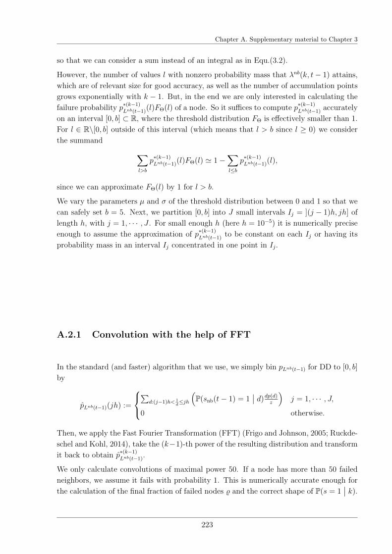
Chapter A. Supplementary material to Chapter 3
so that we can consider a sum instead of an integral as in Equ.(3.2).
However, the number of values l with nonzero probability mass that λnb(k, t− 1) attains,
which are of relevant size for good accuracy, as well as the number of accumulation points
grows exponentially with k − 1. But, in the end we are only interested in calculating the
failure probability p∗(k−1)
Lnb(t−1)(l)FΘ(l) of a node. So it suffices to compute p
∗(k−1)
Lnb(t−1)accurately
on an interval [0, b] ⊂ R, where the threshold distribution FΘ is effectively smaller than 1.
For l ∈ R\[0, b] outside of this interval (which means that l > b since l ≥ 0) we consider
the summand ∑l>b
p∗(k−1)
Lnb(t−1)(l)FΘ(l) ' 1−
∑l≤b
p∗(k−1)
Lnb(t−1)(l),
since we can approximate FΘ(l) by 1 for l > b.
We vary the parameters µ and σ of the threshold distribution between 0 and 1 so that we
can safely set b = 5. Next, we partition [0, b] into J small intervals Ij = ](j − 1)h, jh] of
length h, with j = 1, · · · , J . For small enough h (here h = 10−5) it is numerically precise
enough to assume the approximation of p∗(k−1)
Lnb(t−1)to be constant on each Ij or having its
probability mass in an interval Ij concentrated in one point in Ij.
A.2.1 Convolution with the help of FFT
In the standard (and faster) algorithm that we use, we simply bin pLnb(t−1) for DD to [0, b]
by
pLnb(t−1)(jh) :=
∑
d:(j−1)h< 1d≤jh
(P(snb(t− 1) = 1
∣∣ d)dp(d)z
)j = 1, · · · , J,
0 otherwise.
Then, we apply the Fast Fourier Transformation (FFT) (Frigo and Johnson, 2005; Ruckde-
schel and Kohl, 2014), take the (k−1)-th power of the resulting distribution and transform
it back to obtain p∗(k−1)
Lnb(t−1).
We only calculate convolutions of maximal power 50. If a node has more than 50 failed
neighbors, we assume it fails with probability 1. This is numerically accurate enough for
the calculation of the final fraction of failed nodes % and the correct shape of P(s = 1∣∣ k).
223
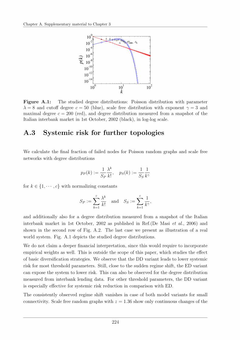
Chapter A. Supplementary material to Chapter 3
100
101
102
k
10-14
10-12
10-10
10-8
10-6
10-4
10-2
100
p(k)
Figure A.1: The studied degree distributions: Poisson distribution with parameterλ = 8 and cutoff degree c = 50 (blue), scale free distribution with exponent γ = 3 andmaximal degree c = 200 (red), and degree distribution measured from a snapshot of theItalian interbank market in 1st October, 2002 (black), in log-log scale.
A.3 Systemic risk for further topologies
We calculate the final fraction of failed nodes for Poisson random graphs and scale free
networks with degree distributions
pP (k) :=1
SP
λk
k!, pS(k) :=
1
SS
1
kγ
for k ∈ 1, · · · , c with normalizing constants
SP :=c∑
k=1
λk
k!and SS :=
c∑k=1
1
kγ,
and additionally also for a degree distribution measured from a snapshot of the Italian
interbank market in 1st October, 2002 as published in Ref.(De Masi et al., 2006) and
shown in the second row of Fig. A.2. The last case we present as illustration of a real
world system. Fig. A.1 depicts the studied degree distributions.
We do not claim a deeper financial interpretation, since this would require to incorporate
empirical weights as well. This is outside the scope of this paper, which studies the effect
of basic diversification strategies. We observe that the DD variant leads to lower systemic
risk for most threshold parameters. Still, close to the sudden regime shift, the ED variant
can expose the system to lower risk. This can also be observed for the degree distribution
measured from interbank lending data. For other threshold parameters, the DD variant
is especially effective for systemic risk reduction in comparison with ED.
The consistently observed regime shift vanishes in case of both model variants for small
connectivity. Scale free random graphs with z = 1.36 show only continuous changes of the
224
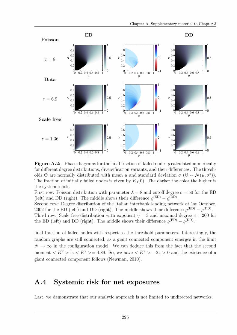
Chapter A. Supplementary material to Chapter 3
ED DDPoisson
z = 8
µ
σ
0 0.2 0.4 0.6 0.8 10
0.2
0.4
0.6
0.8
1
0
0.5
1
µ
σ
0 0.2 0.4 0.6 0.8 10
0.2
0.4
0.6
0.8
1
−1
0
1
µ
σ
0 0.2 0.4 0.6 0.8 10
0.2
0.4
0.6
0.8
1
0
0.5
1
Data
z = 6.9
µ
σ
0 0.2 0.4 0.6 0.8 10
0.2
0.4
0.6
0.8
1
0
0.5
1
µσ
0 0.2 0.4 0.6 0.8 10
0.2
0.4
0.6
0.8
1
−1
0
1
µ
σ
0 0.2 0.4 0.6 0.8 10
0.2
0.4
0.6
0.8
1
0
0.5
1
Scale free
z = 1.36
µ
σ
0 0.2 0.4 0.6 0.8 10
0.2
0.4
0.6
0.8
1
0
0.5
1
µ
σ
0 0.2 0.4 0.6 0.8 10
0.2
0.4
0.6
0.8
1
−1
0
1
µ
σ
0 0.2 0.4 0.6 0.8 10
0.2
0.4
0.6
0.8
1
0
0.5
1
Figure A.2: Phase diagrams for the final fraction of failed nodes % calculated numericallyfor different degree distributions, diversification variants, and their differences. The thresh-olds Θ are normally distributed with mean µ and standard deviation σ (Θ ∼ N (µ, σ2)).The fraction of initially failed nodes is given by FΘ(0). The darker the color the higher isthe systemic risk.First row: Poisson distribution with parameter λ = 8 and cutoff degree c = 50 for the ED(left) and DD (right). The middle shows their difference %(ED) − %(DD).Second row: Degree distribution of the Italian interbank lending network at 1st October,2002 for the ED (left) and DD (right). The middle shows their difference %(ED) − %(DD).Third row: Scale free distribution with exponent γ = 3 and maximal degree c = 200 forthe ED (left) and DD (right). The middle shows their difference %(ED) − %(DD).
final fraction of failed nodes with respect to the threshold parameters. Interestingly, the
random graphs are still connected, as a giant connected component emerges in the limit
N → ∞ in the configuration model. We can deduce this from the fact that the second
moment < K2 > is < K2 >= 4.89. So, we have < K2 > −2z > 0 and the existence of a
giant connected component follows (Newman, 2010).
A.4 Systemic risk for net exposures
Last, we demonstrate that our analytic approach is not limited to undirected networks.
225
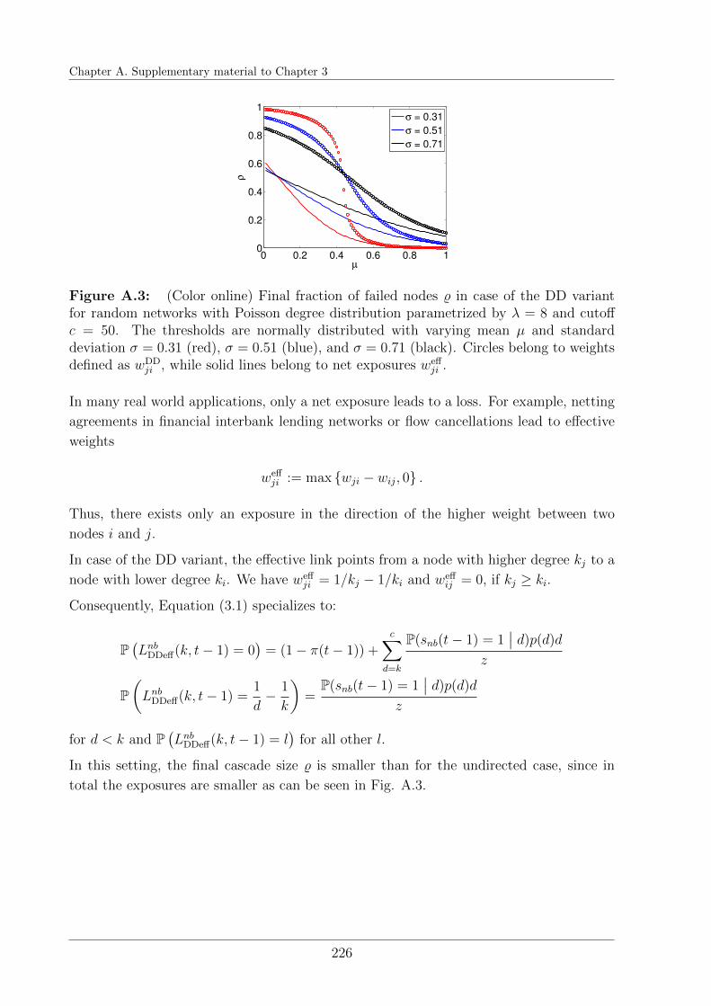
Chapter A. Supplementary material to Chapter 3
0 0.2 0.4 0.6 0.8 10
0.2
0.4
0.6
0.8
1
µ
ρ
σ = 0.31
σ = 0.51
σ = 0.71
Figure A.3: (Color online) Final fraction of failed nodes % in case of the DD variantfor random networks with Poisson degree distribution parametrized by λ = 8 and cutoffc = 50. The thresholds are normally distributed with varying mean µ and standarddeviation σ = 0.31 (red), σ = 0.51 (blue), and σ = 0.71 (black). Circles belong to weightsdefined as wDD
ji , while solid lines belong to net exposures weffji .
In many real world applications, only a net exposure leads to a loss. For example, netting
agreements in financial interbank lending networks or flow cancellations lead to effective
weights
weffji := max wji − wij, 0 .
Thus, there exists only an exposure in the direction of the higher weight between two
nodes i and j.
In case of the DD variant, the effective link points from a node with higher degree kj to a
node with lower degree ki. We have weffji = 1/kj − 1/ki and weff
ij = 0, if kj ≥ ki.
Consequently, Equation (3.1) specializes to:
P(LnbDDeff(k, t− 1) = 0
)= (1− π(t− 1)) +
c∑d=k
P(snb(t− 1) = 1∣∣ d)p(d)d
z
P(LnbDDeff(k, t− 1) =
1
d− 1
k
)=
P(snb(t− 1) = 1∣∣ d)p(d)d
z
for d < k and P(LnbDDeff(k, t− 1) = l
)for all other l.
In this setting, the final cascade size % is smaller than for the undirected case, since in
total the exposures are smaller as can be seen in Fig. A.3.
226
Chapter B. Supplementary material to Chapter 9
Appendix B
Supplementary material to Chapter 9
Proof of Equation (9.2) for fully connected networks
The probabilistic inclusion-exclusion principle Szpankowski (2001) states that for events
A1, . . . , An in an arbitrary probability space, at least one of these events occurs with
probability:
P
(n⋃j=1
Aj
)=
n∑j=1
(−1)j+1∑Ij
P
⋂l∈Ij
Al
where Ij = l1, . . . , lj is a set containing exactly j distinct indicees li ∈ 1, . . . , n. In
case that the probability qj = P(⋂
l∈Ij Al
)only depends on the number j of events that
are intersected, we have
P
(n⋃j=1
Aj
)=
n∑j=1
(−1)j(n
j
)qj,
as there exist(nj
)different subsets of 1, . . . , n with j elements.
To proof Equation (9.2) we need to define appropriate events Aj so that pn = P(⋃n
j=1Aj
)and qj = F (λ[n− j])j pn−j, where we associate index j with j = n − l. Then Equation
(9.2) follows immediately from the stated principle.
First, we recall that pn is the probability that n fully connected nodes fail in a cascade
process considering only these n nodes (so that none of the failures is additionally influ-
enced by other nodes in the network). There are several threshold configurations that lead
to this outcome. All of them are of the form that some n− j nodes have failed first, while
the remaining j nodes fail because of the n− j failures before.
227

Chapter B. Supplementary material to Chapter 9
Each Aj subsumes events where the same j specific nodes i1, . . . , ij have thresholds smaller
than λ[n−j] and the remaining n−j nodes failed in a cascade without considering i1, . . . , ij.
Indeed, the union of all Aj coincides with all cascades of size n and each Aj occurs with
probability qj.
228
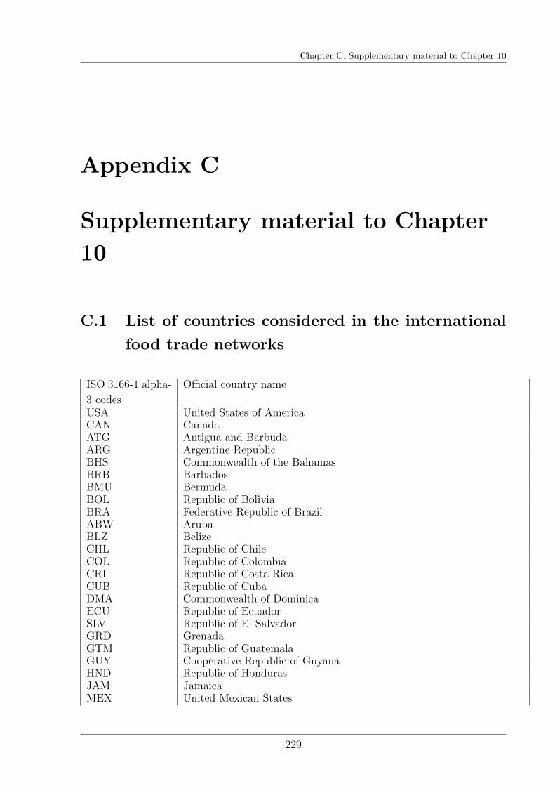
Chapter C. Supplementary material to Chapter 10
Appendix C
Supplementary material to Chapter
10
C.1 List of countries considered in the international
food trade networks
ISO 3166-1 alpha-
3 codes
Official country name
USA United States of AmericaCAN CanadaATG Antigua and BarbudaARG Argentine RepublicBHS Commonwealth of the BahamasBRB BarbadosBMU BermudaBOL Republic of BoliviaBRA Federative Republic of BrazilABW ArubaBLZ BelizeCHL Republic of ChileCOL Republic of ColombiaCRI Republic of Costa RicaCUB Republic of CubaDMA Commonwealth of DominicaECU Republic of EcuadorSLV Republic of El SalvadorGRD GrenadaGTM Republic of GuatemalaGUY Cooperative Republic of GuyanaHND Republic of HondurasJAM JamaicaMEX United Mexican States
229

Chapter C. Supplementary material to Chapter 10
MSR MontserratNIC Republic of NicaraguaPAN Republic of PanamaPRY Republic of ParaguayPER Republic of PeruKNA Federation of Saint Kitts and NevisLCA Saint LuciaVCT Saint Vincent and the GrenadinesSUR Republic of SurinameTTO Republic of Trinidad and TobagoURY Oriental Republic of UruguayVEN Bolivarian Republic of VenezuelaAUT Republic of AustriaDNK Kingdom of DenmarkFRO Fxoroyar (Faroe Is.)FIN Republic of FinlandFRA French RepublicDEU Federal Republic of GermanyGRC Hellenic RepublicISL Republic of IcelandIRL IrelandITA Italian RepublicMLT Republic of MaltaNLD Kingdom of the NetherlandsNOR Kingdom of NorwayPRT Portuguese RepublicESP Kingdom of SpainSWE Kingdom of SwedenCHE Swiss ConfederationGBR United Kingdom of Great Britain and Northern IrelandGRL GreenlandBELLUX the Kingdom of Belgium and the Grand Duchy of Luxembourg combinedREU ReunionALB Republic of AlbaniaBGR the Republic of BulgariaCYP Republic of CyprusEST Republic of EstoniaBIH Bosnia and HerzegovinaHUN Republic of HungaryHRV Republic of CroatiaLVA Republic of LatviaLTU Republic of LithuaniaMKD Republic of MacedoniaCZE Czech RepublicPOL Republic of PolandROU RomaniaSVN Republic of SloveniaSVK Slovak RepublicTUR Republic of TurkeySRB Republic of Serbia
230

Chapter C. Supplementary material to Chapter 10
MNE MontenegroARM Republic of ArmeniaAZE Republic of AzerbaijanBLR Republic of BelarusGEO GeorgiaMDA Republic of MoldovaRUS Russian FederationUKR UkraineCHN People’s Republic of ChinaHKG Hong Kong Special Administrative RegionJPN JapanKOR Republic of KoreaMAC Macau Special Administrative RegionMNG MongoliaTWN Taiwan, the Republic of ChinaKAZ Republic of KazakhstanKGZ Kyrgyz RepublicAFG Islamic State of AfghanistanBGD People’s Republic of BangladeshBTN Kingdom of BhutanLKA Democratic Socialist Republic of Sri LankaIND Republic of IndiaIRN Islamic Republic of IranMDV Republic of MaldivesNPL Kingdom of NepalPAK Islamic Republic of PakistanBRN Negara Brunei DarussalamIDN Republic of IndonesiaKHM Kingdom of CambodiaMYS MalaysiaPHL Republic of the PhilippinesSGP Republic of SingaporeTHA Kingdom of ThailandBHR State of BahrainQAT State of QatarSAU Kingdom of Saudi ArabiaOMN Sultanate of OmanARE the United Arab EmiratesYEM Republic of YemenJOR Hashemite Kingdom of JordanKWT State of KuwaitLBN Lebanese RepublicSYR Syrian Arab RepublicISR State of IsraelDZA People’s Democratic Republic of AlgeriaEGY Arab Republic of EgyptLBY Great Socialist People’s Libyan Arab JamahiriyaMAR Kingdom of MoroccoSDN Republic of the SudanTUN Republic of Tunisia
231

Chapter C. Supplementary material to Chapter 10
CMR Republic of CameroonCPV Republic of Cape VerdeCAF Central African RepublicCOG Republic of the CongoGAB Gabonese RepublicSTP Democratic Republic of Sao Tome and PrincipeCOD Democratic Republic of the CongoBEN Republic of BeninGMB Republic of the GambiaGHA Republic of GhanaGIN Republic of GuineaCIV Republic of Cote D’IvoireMLI Republic of MaliMRT Islamic Republic of MauritaniaNER Republic of NigerNGA Federal Republic of NigeriaSEN Republic of SenegalSLE Republic of Sierra LeoneTGO Togolese RepublicBFA Burkina FasoBDI Republic of BurundiKEN Republic of KenyaRWA Rwandese RepublicUGA the Republic of UgandaETH Federal Democratic Republic of EthiopiaBWA Republic of BotswanaMWI Republic of MalawiNAM Republic of NamibiaZWE Republic of ZimbabweZAF Republic of South AfricaSWZ Kingdom of SwazilandTZA United Republic of TanzaniaZMB Republic of ZambiaCOM Federal Islamic Republic of the ComorosMDG Republic of MadagascarMUS Republic of MauritiusSYC Republic of SeychellesAUS Commonwealth of AustraliaSLB Solomon IslandsCOK the Cook IslandsFJI Republic of the Fiji IslandsPYF Territory of French PolynesiaKIR Republic of KiribatiNCL Territory of New Caledonia and DependenciesVUT Republic of VanuatuNZL New ZealandPNG Independent State of Papua New GuineaTON Kingdom of TongaTUV TuvaluGUF French Guiana
232
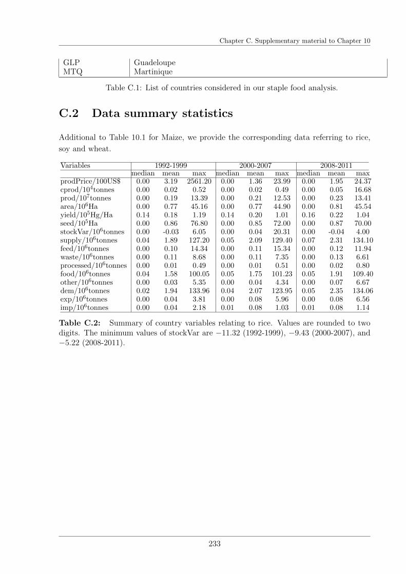
Chapter C. Supplementary material to Chapter 10
GLP GuadeloupeMTQ Martinique
Table C.1: List of countries considered in our staple food analysis.
C.2 Data summary statistics
Additional to Table 10.1 for Maize, we provide the corresponding data referring to rice,
soy and wheat.
Variables 1992-1999 2000-2007 2008-2011median mean max median mean max median mean max
prodPrice/100US$ 0.00 3.19 2561.20 0.00 1.36 23.99 0.00 1.95 24.37cprod/104tonnes 0.00 0.02 0.52 0.00 0.02 0.49 0.00 0.05 16.68prod/107tonnes 0.00 0.19 13.39 0.00 0.21 12.53 0.00 0.23 13.41area/106Ha 0.00 0.77 45.16 0.00 0.77 44.90 0.00 0.81 45.54yield/105Hg/Ha 0.14 0.18 1.19 0.14 0.20 1.01 0.16 0.22 1.04seed/105Ha 0.00 0.86 76.80 0.00 0.85 72.00 0.00 0.87 70.00stockVar/106tonnes 0.00 -0.03 6.05 0.00 0.04 20.31 0.00 -0.04 4.00supply/106tonnes 0.04 1.89 127.20 0.05 2.09 129.40 0.07 2.31 134.10feed/106tonnes 0.00 0.10 14.34 0.00 0.11 15.34 0.00 0.12 11.94waste/106tonnes 0.00 0.11 8.68 0.00 0.11 7.35 0.00 0.13 6.61processed/106tonnes 0.00 0.01 0.49 0.00 0.01 0.51 0.00 0.02 0.80food/106tonnes 0.04 1.58 100.05 0.05 1.75 101.23 0.05 1.91 109.40other/106tonnes 0.00 0.03 5.35 0.00 0.04 4.34 0.00 0.07 6.67dem/106tonnes 0.02 1.94 133.96 0.04 2.07 123.95 0.05 2.35 134.06exp/106tonnes 0.00 0.04 3.81 0.00 0.08 5.96 0.00 0.08 6.56imp/106tonnes 0.00 0.04 2.18 0.01 0.08 1.03 0.01 0.08 1.14
Table C.2: Summary of country variables relating to rice. Values are rounded to twodigits. The minimum values of stockVar are −11.32 (1992-1999), −9.43 (2000-2007), and−5.22 (2008-2011).
233
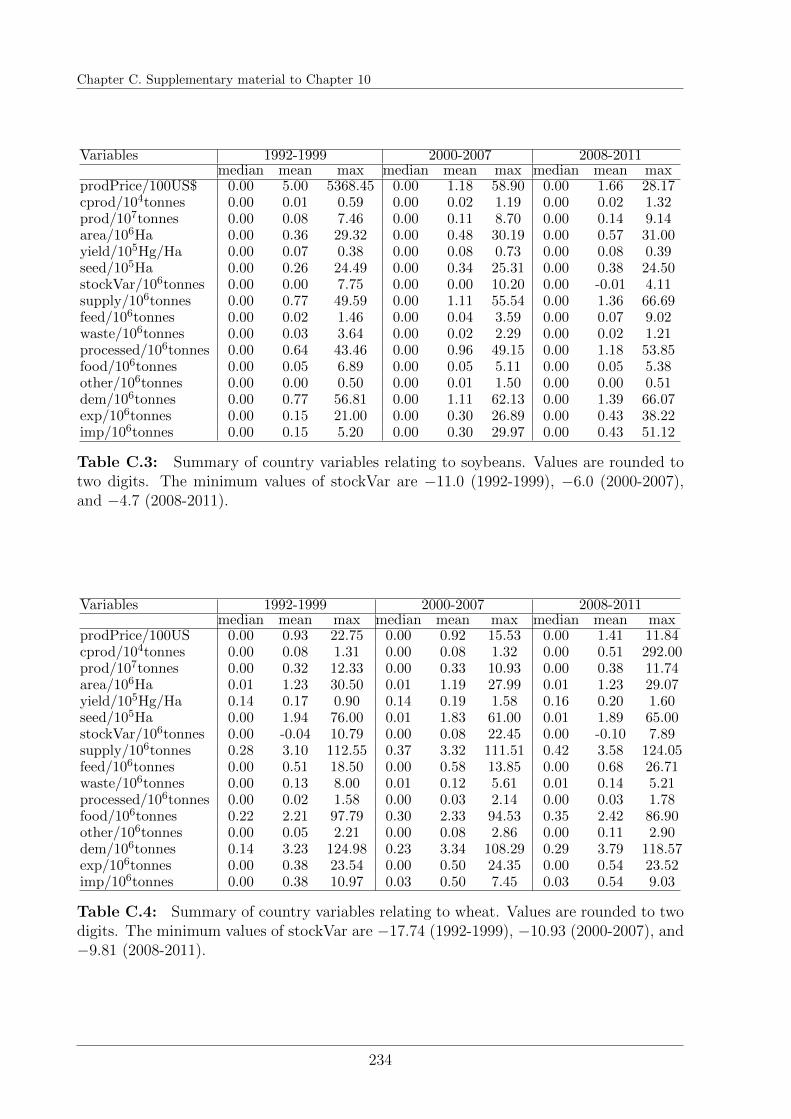
Chapter C. Supplementary material to Chapter 10
Variables 1992-1999 2000-2007 2008-2011median mean max median mean max median mean max
prodPrice/100US$ 0.00 5.00 5368.45 0.00 1.18 58.90 0.00 1.66 28.17cprod/104tonnes 0.00 0.01 0.59 0.00 0.02 1.19 0.00 0.02 1.32prod/107tonnes 0.00 0.08 7.46 0.00 0.11 8.70 0.00 0.14 9.14area/106Ha 0.00 0.36 29.32 0.00 0.48 30.19 0.00 0.57 31.00yield/105Hg/Ha 0.00 0.07 0.38 0.00 0.08 0.73 0.00 0.08 0.39seed/105Ha 0.00 0.26 24.49 0.00 0.34 25.31 0.00 0.38 24.50stockVar/106tonnes 0.00 0.00 7.75 0.00 0.00 10.20 0.00 -0.01 4.11supply/106tonnes 0.00 0.77 49.59 0.00 1.11 55.54 0.00 1.36 66.69feed/106tonnes 0.00 0.02 1.46 0.00 0.04 3.59 0.00 0.07 9.02waste/106tonnes 0.00 0.03 3.64 0.00 0.02 2.29 0.00 0.02 1.21processed/106tonnes 0.00 0.64 43.46 0.00 0.96 49.15 0.00 1.18 53.85food/106tonnes 0.00 0.05 6.89 0.00 0.05 5.11 0.00 0.05 5.38other/106tonnes 0.00 0.00 0.50 0.00 0.01 1.50 0.00 0.00 0.51dem/106tonnes 0.00 0.77 56.81 0.00 1.11 62.13 0.00 1.39 66.07exp/106tonnes 0.00 0.15 21.00 0.00 0.30 26.89 0.00 0.43 38.22imp/106tonnes 0.00 0.15 5.20 0.00 0.30 29.97 0.00 0.43 51.12
Table C.3: Summary of country variables relating to soybeans. Values are rounded totwo digits. The minimum values of stockVar are −11.0 (1992-1999), −6.0 (2000-2007),and −4.7 (2008-2011).
Variables 1992-1999 2000-2007 2008-2011median mean max median mean max median mean max
prodPrice/100US 0.00 0.93 22.75 0.00 0.92 15.53 0.00 1.41 11.84cprod/104tonnes 0.00 0.08 1.31 0.00 0.08 1.32 0.00 0.51 292.00prod/107tonnes 0.00 0.32 12.33 0.00 0.33 10.93 0.00 0.38 11.74area/106Ha 0.01 1.23 30.50 0.01 1.19 27.99 0.01 1.23 29.07yield/105Hg/Ha 0.14 0.17 0.90 0.14 0.19 1.58 0.16 0.20 1.60seed/105Ha 0.00 1.94 76.00 0.01 1.83 61.00 0.01 1.89 65.00stockVar/106tonnes 0.00 -0.04 10.79 0.00 0.08 22.45 0.00 -0.10 7.89supply/106tonnes 0.28 3.10 112.55 0.37 3.32 111.51 0.42 3.58 124.05feed/106tonnes 0.00 0.51 18.50 0.00 0.58 13.85 0.00 0.68 26.71waste/106tonnes 0.00 0.13 8.00 0.01 0.12 5.61 0.01 0.14 5.21processed/106tonnes 0.00 0.02 1.58 0.00 0.03 2.14 0.00 0.03 1.78food/106tonnes 0.22 2.21 97.79 0.30 2.33 94.53 0.35 2.42 86.90other/106tonnes 0.00 0.05 2.21 0.00 0.08 2.86 0.00 0.11 2.90dem/106tonnes 0.14 3.23 124.98 0.23 3.34 108.29 0.29 3.79 118.57exp/106tonnes 0.00 0.38 23.54 0.00 0.50 24.35 0.00 0.54 23.52imp/106tonnes 0.00 0.38 10.97 0.03 0.50 7.45 0.03 0.54 9.03
Table C.4: Summary of country variables relating to wheat. Values are rounded to twodigits. The minimum values of stockVar are −17.74 (1992-1999), −10.93 (2000-2007), and−9.81 (2008-2011).
234

List of figures
List of Figures
2.1 Example. Graphical representation of an undirected network, an undirected network inter-
preted as directed network, and a directed network. Nodes are depicted by circles, while
undirected links are drawn as lines between nodes. A directed link (i, j) is represented by
an arrow that points from the first node i to the second node j of the link. The degree k1
of node 1 is k1 = 2 in all cases and its out-degree is kout1 = 2 as well in the right plot. . . . 13
2.2 General set-up for the visualization of examples to explain several load distribution mech-
anisms. The figure is a slight modification of Fig. 1 by Lorenz et al. (2009). . . . . . . . . 15
2.3 Left Column: Example for a cascade with CL ED load distribution (left) and CL DD load
distribution (right) mechanism starting from the set-up in Fig. 2.2. The initial load is set to
λ0 = 0. The figure is a slight modification of Fig. 2 by Lorenz et al. (2009). Right Column:
Example for a cascade with OLRD LLSC load distribution (left) and OLRD LLSS load
distribution (right) mechanism starting from the set-up in Fig. 2.2. The initial load is set
to λ0 = 1. The figure is a slight modification of Fig. 4 by Lorenz et al. (2009). . . . . . . 19
2.4 Example for a cascade with LRD LLSC load distribution (left) and LRD LLSS load dis-
tribution (right) mechanism starting from the set-up in Fig. 2.2. The initial load is set to
λ0 = 1. The figure is a slight modification of Fig. 3 by Lorenz et al. (2009). . . . . . . . . 21
2.5 Visualization of the construction of a network according to the configuration model. Stubs
represent final node degrees. . . . . . . . . . . . . . . . . . . . . . . . . . . . . . . . . . . . 25
2.6 (a) The studied degree distributions: Poisson distribution with parameter λ = 2.82 and
cutoff degree c = 50 (black), scale free distribution with exponent γ = 3 and maximal degree
c = 200 and average degree z = 3 (purple) in log-log scale. (b) The corresponding degree
sequences of simulated networks with size N = 105 nodes in the same colors as in (a). . . 26
2.7 Visualization of correlation schemes between threshold and degree distribution in a network
with N = 105 nodes and Poisson degree sequence (with z = 3). The thresholds follow
the order statistics of a normal distribution with mean µ = 0.5 and σ = 0.5, i.e. Θ ∼N(0.5, 0.52
). Nodes with thresholds as indicated by the histogram have degrees defined by
the color of the bars: (a) peripheral failures (pf), (b) central failures (cf). . . . . . . . . . 29
2.8 Phase diagram for the initial fraction of failed nodes %0 = %(0) in an infinite network with
normally distributed thresholds (Θ ∼ N (µ, σ2)). %0 is constant along the lines σ = µ/Φ−1(%0). 30
235
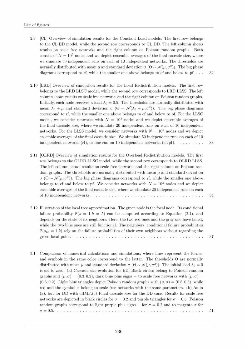
List of figures
2.9 [CL] Overview of simulation results for the Constant Load models. The first row belongs
to the CL ED model, while the second row corresponds to CL DD. The left column shows
results on scale free networks and the right column on Poisson random graphs. Both
consist of N = 105 nodes and we depict ensemble averages of the final cascade size, where
we simulate 50 independent runs on each of 10 independent networks. The thresholds are
normally distributed with mean µ and standard deviation σ (Θ ∼ N (µ, σ2)). The big phase
diagrams correspond to rf, while the smaller one above belongs to cf and below to pf. . . . 32
2.10 [LRD] Overview of simulation results for the Load Redistribution models. The first row
belongs to the LRD LLSC model, while the second row corresponds to LRD LLSS. The left
column shows results on scale free networks and the right column on Poisson random graphs.
Initially, each node receives a load λ0 = 0.5. The thresholds are normally distributed with
mean λ0 + µ and standard deviation σ (Θ ∼ N (λ0 + µ, σ2)). The big phase diagrams
correspond to rf, while the smaller one above belongs to cf and below to pf. For the LLSC
model, we consider networks with N = 103 nodes and we depict ensemble averages of
the final cascade size, where we simulate 20 independent runs on each of 10 independent
networks. For the LLSS model, we consider networks with N = 105 nodes and we depict
ensemble averages of the final cascade size. We simulate 50 independent runs on each of 10
independent networks (rf), or one run on 10 independent networks (cf/pf). . . . . . . . . 33
2.11 [OLRD] Overview of simulation results for the Overload Redistribution models. The first
row belongs to the OLRD LLSC model, while the second row corresponds to OLRD LLSS.
The left column shows results on scale free networks and the right column on Poisson ran-
dom graphs. The thresholds are normally distributed with mean µ and standard deviation
σ (Θ ∼ N (µ, σ2)). The big phase diagrams correspond to rf, while the smaller one above
belongs to cf and below to pf. We consider networks with N = 103 nodes and we depict
ensemble averages of the final cascade size, where we simulate 20 independent runs on each
of 10 independent networks. . . . . . . . . . . . . . . . . . . . . . . . . . . . . . . . . . . 34
2.12 Illustration of the local tree approximation. The green node is the focal node. Its conditional
failure probability P(s = 1|k = 5) can be computed according to Equation (2.1), and
depends on the state of its neighbors: Here, the two red ones and the gray one have failed,
while the two blue ones are still functional. The neighbors’ conditional failure probabilities
P(snb = 1|k) rely on the failure probabilities of their own neighbors without regarding the
green focal point. . . . . . . . . . . . . . . . . . . . . . . . . . . . . . . . . . . . . . . . . . 37
3.1 Comparison of numerical calculations and simulations, where lines represent the former
and symbols in the same color correspond to the latter. The thresholds Θ are normally
distributed with mean µ and standard deviation σ (Θ ∼ N (µ, σ2)). The initial load λ0 = 0
is set to zero. (a) Cascade size evolution for ED: Black circles belong to Poisson random
graphs and (µ, σ) = (0.3, 0.2), dark blue plus signs + to scale free networks with (µ, σ) =
(0.3, 0.2). Light blue triangles depict Poisson random graphs with (µ, σ) = (0.5, 0.5), while
red and the symbol x belong to scale free networks with the same parameters. (b) As in
(a), but for DD with cHMF.(c) Final cascade size for the DD case. Results for scale free
networks are depicted in black circles for σ = 0.2 and purple triangles for σ = 0.5. Poisson
random graphs correspond to light purple plus signs + for σ = 0.2 and to magenta x for
σ = 0.5. . . . . . . . . . . . . . . . . . . . . . . . . . . . . . . . . . . . . . . . . . . . . . . 51
236
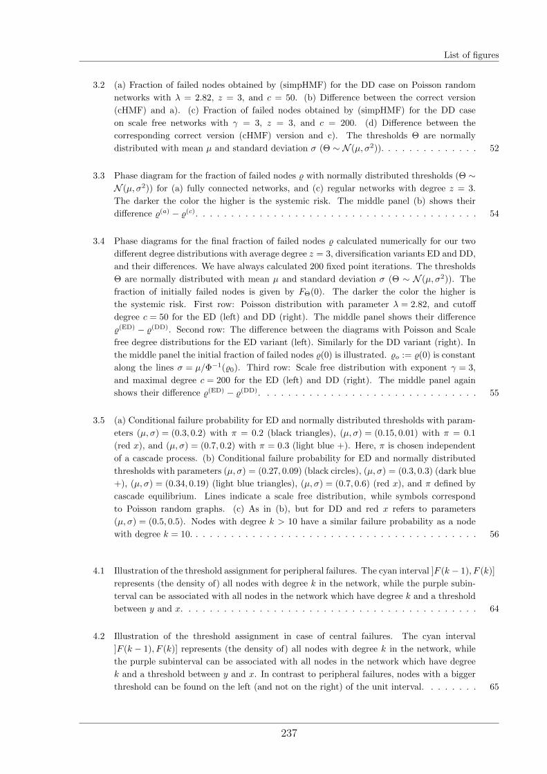
List of figures
3.2 (a) Fraction of failed nodes obtained by (simpHMF) for the DD case on Poisson random
networks with λ = 2.82, z = 3, and c = 50. (b) Difference between the correct version
(cHMF) and a). (c) Fraction of failed nodes obtained by (simpHMF) for the DD case
on scale free networks with γ = 3, z = 3, and c = 200. (d) Difference between the
corresponding correct version (cHMF) version and c). The thresholds Θ are normally
distributed with mean µ and standard deviation σ (Θ ∼ N (µ, σ2)). . . . . . . . . . . . . . 52
3.3 Phase diagram for the fraction of failed nodes % with normally distributed thresholds (Θ ∼N (µ, σ2)) for (a) fully connected networks, and (c) regular networks with degree z = 3.
The darker the color the higher is the systemic risk. The middle panel (b) shows their
difference %(a) − %(c). . . . . . . . . . . . . . . . . . . . . . . . . . . . . . . . . . . . . . . . 54
3.4 Phase diagrams for the final fraction of failed nodes % calculated numerically for our two
different degree distributions with average degree z = 3, diversification variants ED and DD,
and their differences. We have always calculated 200 fixed point iterations. The thresholds
Θ are normally distributed with mean µ and standard deviation σ (Θ ∼ N (µ, σ2)). The
fraction of initially failed nodes is given by FΘ(0). The darker the color the higher is
the systemic risk. First row: Poisson distribution with parameter λ = 2.82, and cutoff
degree c = 50 for the ED (left) and DD (right). The middle panel shows their difference
%(ED) − %(DD). Second row: The difference between the diagrams with Poisson and Scale
free degree distributions for the ED variant (left). Similarly for the DD variant (right). In
the middle panel the initial fraction of failed nodes %(0) is illustrated. %o := %(0) is constant
along the lines σ = µ/Φ−1(%0). Third row: Scale free distribution with exponent γ = 3,
and maximal degree c = 200 for the ED (left) and DD (right). The middle panel again
shows their difference %(ED) − %(DD). . . . . . . . . . . . . . . . . . . . . . . . . . . . . . . 55
3.5 (a) Conditional failure probability for ED and normally distributed thresholds with param-
eters (µ, σ) = (0.3, 0.2) with π = 0.2 (black triangles), (µ, σ) = (0.15, 0.01) with π = 0.1
(red x), and (µ, σ) = (0.7, 0.2) with π = 0.3 (light blue +). Here, π is chosen independent
of a cascade process. (b) Conditional failure probability for ED and normally distributed
thresholds with parameters (µ, σ) = (0.27, 0.09) (black circles), (µ, σ) = (0.3, 0.3) (dark blue
+), (µ, σ) = (0.34, 0.19) (light blue triangles), (µ, σ) = (0.7, 0.6) (red x), and π defined by
cascade equilibrium. Lines indicate a scale free distribution, while symbols correspond
to Poisson random graphs. (c) As in (b), but for DD and red x refers to parameters
(µ, σ) = (0.5, 0.5). Nodes with degree k > 10 have a similar failure probability as a node
with degree k = 10. . . . . . . . . . . . . . . . . . . . . . . . . . . . . . . . . . . . . . . . . 56
4.1 Illustration of the threshold assignment for peripheral failures. The cyan interval ]F (k − 1), F (k)]
represents (the density of) all nodes with degree k in the network, while the purple subin-
terval can be associated with all nodes in the network which have degree k and a threshold
between y and x. . . . . . . . . . . . . . . . . . . . . . . . . . . . . . . . . . . . . . . . . . 64
4.2 Illustration of the threshold assignment in case of central failures. The cyan interval
]F (k − 1), F (k)] represents (the density of) all nodes with degree k in the network, while
the purple subinterval can be associated with all nodes in the network which have degree
k and a threshold between y and x. In contrast to peripheral failures, nodes with a bigger
threshold can be found on the left (and not on the right) of the unit interval. . . . . . . . 65
237

List of figures
4.3 Comparison of numerical calculations and simulations, where lines represent the former
and symbols in the same color correspond to the latter. We compute T = 50 fixed point
iterations and compare with simulations on networks of size N = 105. The thresholds Θ
are normally distributed with mean µ and standard deviation σ (Θ ∼ N (µ, σ2)). (a) Final
cascade size for pf: Results for scale free networks and σ = 0.5 are depicted in in light blue
triangles for the ED model and in red x for the DD model. Poisson random graphs and
σ = 0.2 correspond to black circles for ED and to dark blue plus signs + for DD. (b) As in
(a), but for cf. . . . . . . . . . . . . . . . . . . . . . . . . . . . . . . . . . . . . . . . . . . 66
4.4 Phase diagrams for the final fraction of failed nodes % calculated numerically according to
a LTA for our two different degree distributions with average degree z = 3, diversification
variants ED and DD, and threshold allocation schemes pf or cf. SF stands for scale free
random networks, while Poisson indicates Poisson random graphs. We have always calcu-
lated 50 fixed point iterations. The left column presents results for pf and the right column
results for cf. The middle column shows their difference %(pf) − %(cf). . . . . . . . . . . . 67
4.5 Phase diagram for the fraction of failed nodes % with thresholds distributed according to the
order statistics obtained from a normal distribution N (µ, σ2) on scale free random graphs
with average degree z = 3. (a) ED with pf, and (c) DD with cf. The middle panel (b)
shows their difference %(a) − %(b). . . . . . . . . . . . . . . . . . . . . . . . . . . . . . . . . 68
4.6 Fraction of failed nodes P (s(t) = 1; k) with degree k in Poisson random graphs that fail at
the time indicated by the color of the bar. Light blue corresponds to fractions of nodes
that remain functional. Nodes with higher degrees than 20 are omitted (k > 20), as their
fraction is small in comparison to the others. (a) Peripheral failures with ED. (b) Central
failures with DD. The thresholds are normally distributed with parameters µ = 0.2 and
σ = 0.3 . . . . . . . . . . . . . . . . . . . . . . . . . . . . . . . . . . . . . . . . . . . . . . 68
5.1 Comparison of numerical LTA calculations and simulations for the LRD LLSS model and
Poisson random graphs (with average degree z = 3), where lines represent the LTA and
symbols in the same color correspond to simulation results. The thresholds Θ are normally
distributed with mean µ and standard deviation σ (Θ ∼ N (µ, σ2)). The initial load is
λ0 = 0.5. (a) We show the cascade size evolution. Black circles belong to (µ, σ) = (0.3, 0.2),
dark blue plus signs + to (µ, σ) = (0.5, 0.5). Light blue triangles depict (µ, σ) = (0.3, 0.7),
while red and the symbol x belong to (µ, σ) = (0.7, 0.3). (b) Final cascade size after T = 300
fixed point iterations. Black circles belong to σ = 0.2 and light blue triangles to σ = 0.3.
Dark blue plus signs + depict σ = 0.5, while red and the symbol x belong to σ = 0.7. . . 78
5.2 Final fraction of failed nodes % for LRD LLSS after 50 fixed point iterations for Poisson
random graphs (with average degree z = 3) obtained by an LTA. The thresholds are
independently normally distributed with mean µ + λ0 and standard deviation σ (Θ ∼N (µ+ λ0, σ
2)). Thus, the fraction of initial failures is identical for all plots. (a) λ0 = 0.3 ,
(b) λ0 = 0.4 , (c) λ0 = 0.5. . . . . . . . . . . . . . . . . . . . . . . . . . . . . . . . . . . . 79
5.3 Final fraction of failed nodes % (after 200 fixed point iterations) with independently normally
distributed thresholds (Θ ∼ N (µ+λ0, σ2)) for infinitely large networks. (a) Poisson random
graphs (with average degree z = 3) (a) LRD LLSS model on fully connected topology with
λ0 = 0.3, (b) LRD LLSS model on Poisson random graphs with λ0 = 0.3 , (c) CL DD
model on Poisson random graphs. . . . . . . . . . . . . . . . . . . . . . . . . . . . . . . . 79
238
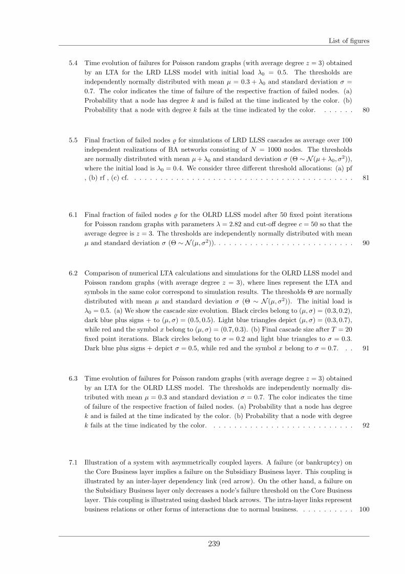
List of figures
5.4 Time evolution of failures for Poisson random graphs (with average degree z = 3) obtained
by an LTA for the LRD LLSS model with initial load λ0 = 0.5. The thresholds are
independently normally distributed with mean µ = 0.3 + λ0 and standard deviation σ =
0.7. The color indicates the time of failure of the respective fraction of failed nodes. (a)
Probability that a node has degree k and is failed at the time indicated by the color. (b)
Probability that a node with degree k fails at the time indicated by the color. . . . . . . 80
5.5 Final fraction of failed nodes % for simulations of LRD LLSS cascades as average over 100
independent realizations of BA networks consisting of N = 1000 nodes. The thresholds
are normally distributed with mean µ+ λ0 and standard deviation σ (Θ ∼ N (µ+ λ0, σ2)),
where the initial load is λ0 = 0.4. We consider three different threshold allocations: (a) pf
, (b) rf , (c) cf. . . . . . . . . . . . . . . . . . . . . . . . . . . . . . . . . . . . . . . . . . . 81
6.1 Final fraction of failed nodes % for the OLRD LLSS model after 50 fixed point iterations
for Poisson random graphs with parameters λ = 2.82 and cut-off degree c = 50 so that the
average degree is z = 3. The thresholds are independently normally distributed with mean
µ and standard deviation σ (Θ ∼ N (µ, σ2)). . . . . . . . . . . . . . . . . . . . . . . . . . . 90
6.2 Comparison of numerical LTA calculations and simulations for the OLRD LLSS model and
Poisson random graphs (with average degree z = 3), where lines represent the LTA and
symbols in the same color correspond to simulation results. The thresholds Θ are normally
distributed with mean µ and standard deviation σ (Θ ∼ N (µ, σ2)). The initial load is
λ0 = 0.5. (a) We show the cascade size evolution. Black circles belong to (µ, σ) = (0.3, 0.2),
dark blue plus signs + to (µ, σ) = (0.5, 0.5). Light blue triangles depict (µ, σ) = (0.3, 0.7),
while red and the symbol x belong to (µ, σ) = (0.7, 0.3). (b) Final cascade size after T = 20
fixed point iterations. Black circles belong to σ = 0.2 and light blue triangles to σ = 0.3.
Dark blue plus signs + depict σ = 0.5, while red and the symbol x belong to σ = 0.7. . . 91
6.3 Time evolution of failures for Poisson random graphs (with average degree z = 3) obtained
by an LTA for the OLRD LLSS model. The thresholds are independently normally dis-
tributed with mean µ = 0.3 and standard deviation σ = 0.7. The color indicates the time
of failure of the respective fraction of failed nodes. (a) Probability that a node has degree
k and is failed at the time indicated by the color. (b) Probability that a node with degree
k fails at the time indicated by the color. . . . . . . . . . . . . . . . . . . . . . . . . . . . 92
7.1 Illustration of a system with asymmetrically coupled layers. A failure (or bankruptcy) on
the Core Business layer implies a failure on the Subsidiary Business layer. This coupling is
illustrated by an inter-layer dependency link (red arrow). On the other hand, a failure on
the Subsidiary Business layer only decreases a node’s failure threshold on the Core Business
layer. This coupling is illustrated using dashed black arrows. The intra-layer links represent
business relations or other forms of interactions due to normal business. . . . . . . . . . . 100
239
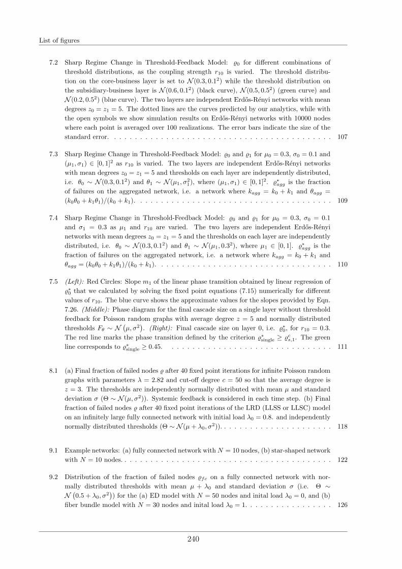
List of figures
7.2 Sharp Regime Change in Threshold-Feedback Model: %0 for different combinations of
threshold distributions, as the coupling strength r10 is varied. The threshold distribu-
tion on the core-business layer is set to N (0.3, 0.12) while the threshold distribution on
the subsidiary-business layer is N (0.6, 0.12) (black curve), N (0.5, 0.52) (green curve) and
N (0.2, 0.52) (blue curve). The two layers are independent Erdos-Renyi networks with mean
degrees z0 = z1 = 5. The dotted lines are the curves predicted by our analytics, while with
the open symbols we show simulation results on Erdos-Renyi networks with 10000 nodes
where each point is averaged over 100 realizations. The error bars indicate the size of the
standard error. . . . . . . . . . . . . . . . . . . . . . . . . . . . . . . . . . . . . . . . . . . 107
7.3 Sharp Regime Change in Threshold-Feedback Model: %0 and %1 for µ0 = 0.3, σ0 = 0.1 and
(µ1, σ1) ∈ [0, 1]2 as r10 is varied. The two layers are independent Erdos-Renyi networks
with mean degrees z0 = z1 = 5 and thresholds on each layer are independently distributed,
i.e. θ0 ∼ N (0.3, 0.12) and θ1 ∼ N (µ1, σ21), where (µ1, σ1) ∈ [0, 1]2. %∗agg is the fraction
of failures on the aggregated network, i.e. a network where kagg = k0 + k1 and θagg =
(k0θ0 + k1θ1)/(k0 + k1). . . . . . . . . . . . . . . . . . . . . . . . . . . . . . . . . . . . . . 109
7.4 Sharp Regime Change in Threshold-Feedback Model: %0 and %1 for µ0 = 0.3, σ0 = 0.1
and σ1 = 0.3 as µ1 and r10 are varied. The two layers are independent Erdos-Renyi
networks with mean degrees z0 = z1 = 5 and the thresholds on each layer are independently
distributed, i.e. θ0 ∼ N (0.3, 0.12) and θ1 ∼ N (µ1, 0.32), where µ1 ∈ [0, 1]. %∗agg is the
fraction of failures on the aggregated network, i.e. a network where kagg = k0 + k1 and
θagg = (k0θ0 + k1θ1)/(k0 + k1). . . . . . . . . . . . . . . . . . . . . . . . . . . . . . . . . . 110
7.5 (Left): Red Circles: Slope m1 of the linear phase transition obtained by linear regression of
%∗0 that we calculated by solving the fixed point equations (7.15) numerically for different
values of r10. The blue curve shows the approximate values for the slopes provided by Eqn.
7.26. (Middle): Phase diagram for the final cascade size on a single layer without threshold
feedback for Poisson random graphs with average degree z = 5 and normally distributed
thresholds Fθ ∼ N(µ, σ2
). (Right): Final cascade size on layer 0, i.e. %∗0, for r10 = 0.3.
The red line marks the phase transition defined by the criterion %∗single ≥ %cs,1. The green
line corresponds to %∗single ≥ 0.45. . . . . . . . . . . . . . . . . . . . . . . . . . . . . . . . 111
8.1 (a) Final fraction of failed nodes % after 40 fixed point iterations for infinite Poisson random
graphs with parameters λ = 2.82 and cut-off degree c = 50 so that the average degree is
z = 3. The thresholds are independently normally distributed with mean µ and standard
deviation σ (Θ ∼ N (µ, σ2)). Systemic feedback is considered in each time step. (b) Final
fraction of failed nodes % after 40 fixed point iterations of the LRD (LLSS or LLSC) model
on an infinitely large fully connected network with initial load λ0 = 0.8. and independently
normally distributed thresholds (Θ ∼ N (µ+ λ0, σ2)). . . . . . . . . . . . . . . . . . . . . . 118
9.1 Example networks: (a) fully connected network withN = 10 nodes, (b) star-shaped network
with N = 10 nodes. . . . . . . . . . . . . . . . . . . . . . . . . . . . . . . . . . . . . . . . . 122
9.2 Distribution of the fraction of failed nodes %fc on a fully connected network with nor-
mally distributed thresholds with mean µ + λ0 and standard deviation σ (i.e. Θ ∼N(0.5 + λ0, σ
2)) for the (a) ED model with N = 50 nodes and inital load λ0 = 0, and (b)
fiber bundle model with N = 30 nodes and inital load λ0 = 1. . . . . . . . . . . . . . . . . 126
240

List of figures
9.3 (a) Final cascade size distribution for fully connected networks of several sizes N obtained
via 104 independent simulations of the CL ED model. The thresholds are independently nor-
mally distributed with mean µ = 0.5 and standard deviation σ = 0.4 (Θ ∼ N(0.5, 0.42
)).
(b) Position of the two local maxima of the distributions in (a) with respect to the network
size N . . . . . . . . . . . . . . . . . . . . . . . . . . . . . . . . . . . . . . . . . . . . . . . . 127
9.4 Distribution of the fraction of failed nodes %∗ on a star-shaped network with N = 50 nodes
for the (a) ED model and (b) DD model. The thresholds are normally distributed with
mean µ = 0.5 and standard deviation σ (i.e. Θ ∼ N(0.5, σ2
). The initial load is λ0 = 0. . 131
9.5 Distribution of the fraction of failed nodes %∗ on a star-shaped network with N = 50
nodes for the LRD LLSS model with λ0 = 1. The thresholds are normally distributed as
Θ ∼ N(µ+ λ0, σ
2). . . . . . . . . . . . . . . . . . . . . . . . . . . . . . . . . . . . . . . . 132
10.1 Color scheme for world countries. Gray color indicates that the country is not considered
in our analyses. . . . . . . . . . . . . . . . . . . . . . . . . . . . . . . . . . . . . . . . . . . 143
10.2 (a) Evolution of the production per capita over time for the four studied staples. (b) Share
of the sum of all reported trades relative to the total production. . . . . . . . . . . . . . . 147
10.3 (a) Gini coefficient of the distribution of positive trade volumes over time. (b) Average
price per tonne of internationally traded crops in US dollars. . . . . . . . . . . . . . . . . 148
10.4 Histogram of the logarithm of the positive trade volumes in the years 1992 and 2013 for
(a) maize, (b) rice, (c) soy, and (d) wheat. . . . . . . . . . . . . . . . . . . . . . . . . . . . 149
10.5 We plot the sum of all productions (i.e., of maize, rice, soy, and wheat) per capita of each
country versus a country’s gross domestic product per capita in 2013. The size of the
bubbles is proportional to the amount of imports. All variables are reported as share of
the maximum observed value. . . . . . . . . . . . . . . . . . . . . . . . . . . . . . . . . . . 150
10.6 [Maize] Evolution of the international maize trade network. Snapshots of the years: (a)
1992, (b) 2000, (c) 2008 and (d) 2013. The color of a link (i, j) corresponds to the exporting
nation i, while the link thickness is proportional to a logarithmic transformation of the
export quantity: log (1 + wij). Links with larger weights are plotted on top of the smaller
ones. Square node shapes indicate that the respective country is a net importer, while
circles refer to net exporters. The node size is proportional to a log transformation of their
net imports or net exports. The twenty biggest nodes have their country code assigned.
Node colors follow the scheme introduced in Fig. 10.1, which encodes regional proximity. . 152
10.7 [Maize] Share of national production in total (world wide) production for the 20 biggest
producers. The segment in darker color refers to the demand of the depicted country. If it
is negative the demand encompasses the sum of both segments, the lighter and the darker
one, and the lighter segment refers to the countries’ production. (a) 1992. (b) 2013. . . . 153
10.8 [Maize] Share of the national variable with respect to the total world wide economic variable
corresponding to maize. The most inner circle belongs to a country’s demand, the second
inner circle corresponds to a country’s export quantity, the second outer circle characterizes
the share of a country’s imports in comparison to the sum of all imports, and the most
outer circle belongs to a country’s share in production. (a) 1992. (b) 2013. . . . . . . . . . 153
10.9 [Maize] Evolution of the five links with the biggest weights (i.e., trade volume) in compar-
ison to the other link weights in the same year. A link is illustrated in the color of the
corresponding exporting nation. The year of reference is (a) 2010. (b) 2013. . . . . . . . . 154
241

List of figures
10.10[Rice] Evolution of the international rice trade network. Snapshots of the years: (a) 1992,
(b) 2000, (c) 2008 and (d) 2013. The color of a link (i, j) corresponds to the exporting
nation i, while the link thickness is proportional to a logarithmic transformation of the
export quantity: log (1 + wij). Links with larger weights are plotted on top of the smaller
ones. Square node shapes indicate that the respective country is a net importer, while
circles refer to net exporters. The node size is proportional to a log transformation of their
net imports or net exports. . . . . . . . . . . . . . . . . . . . . . . . . . . . . . . . . . . . 155
10.11[Rice] Share of national production in total (world wide) production for the 20 biggest
producers. The segment in darker color refers to the demand of the depicted country. If it
is negative the demand encompasses the sum of both segments, the lighter and the darker
one, and the lighter segment refers to the countries’ production. (a) 1992. (b) 2013. . . . 156
10.12[Rice] Share of the national variable with respect to the total world wide economic variable
corresponding to rice. The most inner circle belongs to a country’s demand, the second
inner circle corresponds to a country’s export quantity, the second outer circle characterizes
the share of a country’s imports in comparison to the sum of all imports, and the most
outer circle belongs to a country’s share in production. (a) 1992. (b) 2013. . . . . . . . . . 157
10.13[Rice] Evolution of the five links with the biggest weights (i.e., trade volume) in compar-
ison to the other link weights in the same year. A link is illustrated in the color of the
corresponding exporting nation. The year of reference is (a) 2010. (b) 2013. . . . . . . . . 158
10.14[Soy] Evolution of the international soybean trade network. Snapshots of the years: (a)
1992, (b) 2000, (c) 2008 and (d) 2013. The color of a link (i, j) corresponds to the exporting
nation i, while the link thickness is proportional to a logarithmic transformation of the
export quantity: log (1 + wij). Links with larger weights are plotted on top of the smaller
ones. Square node shapes indicate that the respective country is a net importer, while
circles refer to net exporters. The node size is proportional to a log transformation of their
net imports or net exports. The twenty biggest nodes have their country code assigned.
Node colors follow the scheme introduced in Fig. 10.1, which encodes regional proximity. . 159
10.15[Soy] Share of national production in total (world wide) production for the 20 biggest
producers. The segment in darker color refers to the demand of the depicted country. If it
is negative the demand encompasses the sum of both segments, the lighter and the darker
one, and the lighter segment refers to the countries’ production. (a) 1992. (b) 2013. . . . 160
10.16[Soy] Share of the national variable with respect to the total world wide economic variable
corresponding to rice. The most inner circle belongs to a country’s demand, the second
inner circle corresponds to a country’s export quantity, the second outer circle characterizes
the share of a country’s imports in comparison to the sum of all imports, and the most
outer circle belongs to a country’s share in production. (a) 1992. (b) 2013. . . . . . . . . . 160
10.17[Soy] Evolution of the five links with the biggest weights (i.e., trade volume) in comparison to
the other link weights in the same year. A link is illustrated in the color of the corresponding
exporting nation. The year of reference is (a) 2010. (b) 2013. . . . . . . . . . . . . . . . . 161
242
List of figures
10.18[Wheat] Evolution of the international wheat trade network. Snapshots of the years: (a)
1992, (b) 2000, (c) 2008 and (d) 2013. The color of a link (i, j) corresponds to the exporting
nation i, while the link thickness is proportional to a logarithmic transformation of the
export quantity: log (1 + wij). Links with larger weights are plotted on top of the smaller
ones. Square node shapes indicate that the respective country is a net importer, while
circles refer to net exporters. The node size is proportional to a log transformation of their
net imports or net exports. The twenty biggest nodes have their country code assigned.
Node colors follow the scheme introduced in Fig. 10.1, which encodes regional proximity. . 162
10.19[Wheat] Share of national production in total (world wide) production for the 20 biggest
producers. The segment in darker color refers to the demand of the depicted country. If it
is negative the demand encompasses the sum of both segments, the lighter and the darker
one, and the lighter segment refers to the countries’ production. (a) 1992. (b) 2013. . . . 163
10.20[Wheat] Share of the national variable with respect to the total world wide economic variable
corresponding to rice. The most inner circle belongs to a country’s demand, the second
inner circle corresponds to a country’s export quantity, the second outer circle characterizes
the share of a country’s imports in comparison to the sum of all imports, and the most
outer circle belongs to a country’s share in production. (a) 1992. (b) 2013. . . . . . . . . . 163
10.21[Wheat] Evolution of the five links with the biggest weights (i.e., trade volume) in com-
parison to the other link weights in the same year. A link is illustrated in the color of the
corresponding exporting nation. The year of reference is (a) 2010. (b) 2013. . . . . . . . . 164
11.1 Visualization of aggregated data in 2013 (i.e. trades and variables for maize, rice, soy, and
wheat are added). (a) Production versus demand. The size of the bubbles is proportional to
the inverse average weighted out-degree of a country relative to its exports. All variables are
reported as share of the maximum observed value. (b) Weighted in-degree versus weighted
out-degree. The bubble size corresponds to a country’s demand. . . . . . . . . . . . . . . 174
11.2 [Average shock] (a) Average shock size over time, where shock1 stands for a scenario where
each country is shocked by the same amount sa(c)(y), while shock2 corresponds to shocks
comprising 25% of a country’s the production or demand. (a) Maize, (b) rice, (c) soy, and
(d) wheat. . . . . . . . . . . . . . . . . . . . . . . . . . . . . . . . . . . . . . . . . . . . . . 175
11.3 [Maize] Cascade dependencies for international trade of maize in 2010. Each link corre-
sponds to a shock scenario where the country that passes its color to the link is shocked
initially. Only links with large weights are visible. The link width is proportional to the de-
mand deficit of the country in which the link ends after T = 5·104 cascade steps. Node colors
follow the scheme introduced in Fig. 10.1, which encodes regional proximity. The bar size of
each country represents its weighted degree, i.e. the sum of all in-coming and out-going edge
weights in the cascade dependency network. Shock scenario in case country i is shocked
initially: (a) shocki = sa(m)(2010), (b) shocki = 0.25 max(
prod(m)i (2010),dem
(m)i (2010)
). 177
11.4 Cascade dependencies in 2013. Each link corresponds to a shock scenario where the country
that passes its color to the link is shocked initially by sa(c)(y) as defined in Sec. 11.4. The
link width is proportional to the demand deficit of the country in which the link ends after
T = 5 · 104 cascade steps. Node colors follow the scheme introduced in Fig. 10.1, which
encodes regional proximity. The bar size of each country represents its weighted degree, i.e.
the sum of all in-coming and out-going edge weights in the cascade dependency network.
Considered staples: (a) maize, (b) rice, (c) soy, and (d) wheat. . . . . . . . . . . . . . . . 178
243

List of figures
11.5 [Maize] Systemic risk measures as average over N(y) shocks in each of which a single country
i (with positive demand or production) is shocked according to one of two shock scenarios:
(a) shocki = sa(m)(y), (b) shocki = 0.25 max(prod(m)i (y),dem
(m)i (y)). All measures are
reported as share of the maximal value in the considered time period 1992-2013. The
rounded maximum is given in the legend. . . . . . . . . . . . . . . . . . . . . . . . . . . . 180
11.6 [Maize] Share of countries’ contribution to the depicted risk measures in 2010, i.e., the
amount by which a cascade affects them on average. Maximally T = 5 · 104 cascade steps
are considered. The inner circle corresponds to δ(m), the middle circle to ε(m), and the
outer one to %(m). (a) shock1, (b) shock2. . . . . . . . . . . . . . . . . . . . . . . . . . . . 180
11.7 [Rice] Systemic risk measures as average over N(y) shocks in each of which a single country i
(with positive demand or production) is shocked according to one of two shock scenarios: (a)
shocki = sa(r)(y), (b) shocki = 0.25 max(prod(r)i (y),dem
(r)i (y)). All measures are reported
as share of the maximal value in the considered time period 1992-2013. The rounded
maximum is given in the legend. Maximally T = 5 · 104 cascade steps are considered. . . . 181
11.8 [Rice] Share of countries’ contribution to the depicted risk measures in 2009, i.e., the amount
by which a cascade affects them on average. Maximally T = 5 · 104 cascade steps are
considered. The inner circle corresponds to δ(r), the middle circle to ε(r), and the outer
one to %(r). (a) shock1, (b) shock2. . . . . . . . . . . . . . . . . . . . . . . . . . . . . . . . 182
11.9 [Soy] Systemic risk measures as average over N(y) shocks in each of which a single country i
(with positive demand or production) is shocked according to one of two shock scenarios: (a)
shocki = sa(s)(y), (b) shocki = 0.25 max(prod(s)i (y),dem
(s)i (y)). All measures are reported
as share of the maximal value in the considered time period 1992-2013. The rounded
maximum is given in the legend. Maximally T = 5 · 104 cascade steps are considered. . . . 183
11.10[Soy] Share of countries’ contribution to the depicted risk measures in 2010, i.e., the amount
by which a cascade affects them on average. Maximally T = 5 · 104 cascade steps are
considered. The inner circle corresponds to δ(s), the middle circle to ε(s), and the outer one
to %(s). (a) shock1, (b) shock2. . . . . . . . . . . . . . . . . . . . . . . . . . . . . . . . . . 183
11.11[Wheat] Systemic risk measures as average over N(y) shocks in each of which a single
country i (with positive demand or production) is shocked according to one of two shock
scenarios: (a) shocki = sa(w)(y), (b) shocki = 0.25 max(prod(w)i (y),dem
(w)i (y)). All mea-
sures are reported as share of the maximal value in the considered time period 1992-2013.
The rounded maximum is given in the legend. Maximally T = 5 · 104 cascade steps are
considered. . . . . . . . . . . . . . . . . . . . . . . . . . . . . . . . . . . . . . . . . . . . . 186
11.12[Wheat] Share of countries’ contribution to the depicted risk measures in 2012, i.e., the
amount by which a cascade affects them on average. Maximally T = 5 · 104 cascade steps
are considered. The inner circle corresponds to δ(w), the middle circle to ε(w), and the outer
one to %(w). (a) shock1, (b) shock2. . . . . . . . . . . . . . . . . . . . . . . . . . . . . . . 187
12.1 [Maize] Average world price of one tonne of maize. Black circles and the confidence intervals
correspond to our linear model, while red diamonds depict the observed data. . . . . . . . 194
244
List of figures
12.2 [Maize] Cascade dependencies for the international trade of maize in 2010 corresponding
to a model with observed country preferences. Each link corresponds to a shock scenario
where the country that passes its color to the link is shocked initially. Only links with
large weights are visible. The link width is proportional to the demand deficit of the
country in which the link ends after T = 100 cascade steps. Node colors follow the scheme
introduced in Fig. 10.1, which encodes regional proximity. The bar size of each country
represents its weighted degree, i.e. the sum of all in-coming and out-going edge weights in
the cascade dependency network. Shock scenario in case country i is shocked initially: (a)
shocki = sa(m)(2010), (b) shocki = 0.25 max(
prod(m)i (2010),dem
(m)i (2010)
). . . . . . . . . 199
12.3 [Maize] Evolution of the topological change with respect to two shock types: Black circles
correspond to shock scenario 1, while red diamonds belong to shock scenario 2. The ob-
served network structure and the structure after a shock are compared. The absolute value
of all trade differences for all shocks of single countries is added and shown as fraction of the
total observed trade. (a) Model with observed trade preferences, (b) model with adjusted
trade preferences. . . . . . . . . . . . . . . . . . . . . . . . . . . . . . . . . . . . . . . . . . 203
A.1 The studied degree distributions: Poisson distribution with parameter λ = 8 and cutoff de-
gree c = 50 (blue), scale free distribution with exponent γ = 3 and maximal degree c = 200
(red), and degree distribution measured from a snapshot of the Italian interbank market in
1st October, 2002 (black), in log-log scale. . . . . . . . . . . . . . . . . . . . . . . . . . . . 224
A.2 Phase diagrams for the final fraction of failed nodes % calculated numerically for different
degree distributions, diversification variants, and their differences. The thresholds Θ are
normally distributed with mean µ and standard deviation σ (Θ ∼ N (µ, σ2)). The fraction
of initially failed nodes is given by FΘ(0). The darker the color the higher is the systemic
risk. First row: Poisson distribution with parameter λ = 8 and cutoff degree c = 50 for the
ED (left) and DD (right). The middle shows their difference %(ED) − %(DD). Second row:
Degree distribution of the Italian interbank lending network at 1st October, 2002 for the
ED (left) and DD (right). The middle shows their difference %(ED) − %(DD). Third row:
Scale free distribution with exponent γ = 3 and maximal degree c = 200 for the ED (left)
and DD (right). The middle shows their difference %(ED) − %(DD). . . . . . . . . . . . . . 225
A.3 (Color online) Final fraction of failed nodes % in case of the DD variant for random networks
with Poisson degree distribution parametrized by λ = 8 and cutoff c = 50. The thresholds
are normally distributed with varying mean µ and standard deviation σ = 0.31 (red),
σ = 0.51 (blue), and σ = 0.71 (black). Circles belong to weights defined as wDDji , while
solid lines belong to net exposures weffji . . . . . . . . . . . . . . . . . . . . . . . . . . . . . 226
245

List of tables
List of Tables
10.1 Summary of country variables relating to maize. Values are rounded to two digits. The
minimum values of stockVar are −37.57 (1992-1999), −26.86 (2000-2007), and −8.54 (2008-
2011). . . . . . . . . . . . . . . . . . . . . . . . . . . . . . . . . . . . . . . . . . . . . . . . 145
10.2 Summary of economic country variables. The minimum is zero is all cases because of
missing values. . . . . . . . . . . . . . . . . . . . . . . . . . . . . . . . . . . . . . . . . . . 146
12.1 Regression results. Linear model for the average world price of one tonne of maize: Sum-
mary statistics for the ordinary least squares fit. The data variables have been scaled to
the interval [0,1]. Predictor variables are: total production of maize, rice, and soy. (The
wheat production amount has no significant predictive power), total population, total GDP,
total GDP per capita, production amount of maize per head, standard deviation of maize
productions between all considered countries, total amount of maize that is used for feed,
two indicated interaction terms, and an intercept. . . . . . . . . . . . . . . . . . . . . . . . 196
C.1 List of countries considered in our staple food analysis. . . . . . . . . . . . . . . . . . . . . 233
C.2 Summary of country variables relating to rice. Values are rounded to two digits. The
minimum values of stockVar are −11.32 (1992-1999), −9.43 (2000-2007), and −5.22 (2008-
2011). . . . . . . . . . . . . . . . . . . . . . . . . . . . . . . . . . . . . . . . . . . . . . . . 233
C.3 Summary of country variables relating to soybeans. Values are rounded to two digits. The
minimum values of stockVar are −11.0 (1992-1999), −6.0 (2000-2007), and −4.7 (2008-2011).234
C.4 Summary of country variables relating to wheat. Values are rounded to two digits. The
minimum values of stockVar are −17.74 (1992-1999), −10.93 (2000-2007), and −9.81 (2008-
2011). . . . . . . . . . . . . . . . . . . . . . . . . . . . . . . . . . . . . . . . . . . . . . . . 234
247

List of tables
Glossary
Notation Description Page
ListEW Weighted edge/link set of a weighted graph/network
G = (V,EW ).
13
E Link/edge set of a graph/network G = (V,E). 13G Graph/network G = (V,E) with node/vertex set V
consisting of N nodes and link/edge set E.
12
N Number of nodes in a graph/network G = (V,E).
N := |V |.13
T Time. End of cascade process. T ≤ N − 1. 14V Node/vertex set of a graph/network G = (V,E). 13%N Fraction of failed nodes in a single network of size
N . Cascade size. Measure of systemic risk. Time
dependent. If not stated otherwise %N (T ) is meant.
15
θi Threshold of node i ∈ V . Internal robustness. 14kini In-degree of node i ∈ V . Number of links in G that
point to i.
13
kouti Out-degree of node i ∈ V . Number of links in G that
start in i.
13
ki Degree of node i ∈ V . Number of its network neigh-
bors in G.
13
li Load that a load distributes at failure. Time depen-
dent.
14
lij Load that a failing node i distributes to its neighbor
j. Time dependent.
14
si Binary state of node i ∈ V . si ∈ 0, 1. si = 1
indicates i is failed and si = 0 that i is functional.
It is time dependent. If not stated otherwise si(T ) is
meant.
14
w(DD)ji Weight of link (i, j) in case of Constant Load Damage
Diversification model. w(DD)ji = 1/kj .
17
w(ED)ji Weight of link (i, j) in case of Constant Load Exposure
Diversification model. w(ED)ji = 1/ki.
17
wij Weight of link (i, j). 13zi Net fragility of node i ∈ V . zi := λi − θi. Time
dependent.
14
i, j Indices i, j ∈ 1, · · · , N are often used for nodes in
V .
13
(i, j) Link starting in node i and pointing to node j. 13
249

List of tables
Notation Description Page
Listλi Load that node i carries, fragility, time dependent. If
no time dependence is explicitly stated, the final λi(T )
is meant.
14
λ0 Initial load that a node carries. 14
250
List of tables
Acronyms
Notation Description Page
Listcf central failures 28CL Constant Load 15
DD Damage Diversification 17
ED Exposure Diversification 17
LLSC Local Load Sharing with load Conservation 20LLSS Local Load Sharing with load Shedding 19LRD Load Redistribution 15
OLRD Overload Redistribution 15
pf peripheral failures 28
rf random failures 28
251


Bibliography
Bibliography
Akkermans, H.; Vos, B. (2003). Amplification in Service Supply Chains: An Exploratory Case Study from
the Telecom Industry. Production and Operations Management 12(2), 204–223.
Allen, F.; Carletti, E.; Marquez, R. (2011). Credit Market Competition and Capital Regulation. Review
of Financial Studies 24, 983–1018.
Allen, F.; Gale, D. (2000). Financial Contagion. Journal of Political Economy 108(1), 1–33.
Amihud, Y.; Lev, B. (1981). Risk Reduction as a Managerial Motive for Conglomerate Mergers. The Bell
Journal of Economics 12(2), 605–617.
Amini, H.; Cont, R.; Minca, A. (2010). Resilience to Contagion in Financial Networks. SSRN Electronic
Journal , 1–40.
Amini, H.; Cont, R.; Minca, A. (2012). Stress Testing the Resilience of Financial Networks. International
Journal of Theoretical and Applied Finance 15(01), 1250006.
Arinaminpathy, N.; Kapadia, S.; May, R. M. (2012). Size and complexity in model financial systems.
Proceedings of the National Academy of Sciences of the United States of America 109(45), 18338–
18343.
Aristotle (). Metaphysics. Book H. 1045a 8–10.
Barabasi, A.-L. (2009). Scale-Free Networks: A Decade and Beyond. Science 325(5939), 412–413.
Barabasi, A. L.; Albert, R. (1999). Emergence of Scaling in Random Networks. Science 286(5439),
509–512.
Battiston, S.; Delli Gatti, D.; Gallegati, M.; Greenwald, B.; Stiglitz, J. E. (2012a). Liaisons dangereuses:
Increasing connectivity, risk sharing, and systemic risk. Journal of Economic Dynamics and Control
36(8), 1121–1141.
Battiston, S.; Delli Gatti, D.; Gallegati, M.; Greenwald, B. C. N.; Stiglitz, J. E. (2012b). Credit Default
Cascades: When Does Risk Diversification Increase Stability? Journal of Financial Stability 8, 138–
149.
Battiston, S.; Puliga, M.; Kaushik, R.; Tasca, P.; Caldarelli, G. (2012c). DebtRank: too central to fail?
Financial networks, the FED and systemic risk. Scientific reports 2, 541.
Bikhchandani, S.; Hirshleifer, D.; Welch, I. (1992). A theory of fads, fashion, custom, and cultural change
as informational cascades. Journal of political Economy 100(5), 992–1026.
253
Bibliography
Boss, M.; Elsinger, H.; Summer, M.; 4, S. T. (2004). Network topology of the interbank market. Quanti-
tative Finance 4, 677–684.
Brockmann, D.; Helbing, D. (2013). The Hidden Geometry of Complex, Network-Driven Contagion
Phenomena. Science 342(6164), 1337–1342.
Brummitt, C. D.; D’Souza, R. M.; Leicht, E. a. (2012a). Suppressing cascades of load in interdependent
networks. Proceedings of the National Academy of Sciences of the United States of America 109(12),
E680—-9.
Brummitt, C. D.; Kobayashi, T. (2015). Cascades in multiplex financial networks with debts of different
seniority. Physical Review E 91(6), 62813.
Brummitt, C. D.; Lee, K.-M.; Goh, K.-I. (2012b). Multiplexity-facilitated cascades in networks. Physical
Review E 85(4), 45102.
Buldyrev, S. V.; Parshani, R.; Paul, G.; Stanley, H. E.; Havlin, S. (2010). Catastrophic cascade of failures
in interdependent networks. Nature 464(7291), 1025–1028.
Burkholz, R.; Garas, A.; Schweitzer, F. (2016a). How damage diversification can reduce systemic risk.
Physical Review E 93, 042313.
Burkholz, R.; Leduc, M. V.; Garas, A.; Schweitzer, F. (2016b). Systemic risk in multiplex networks with
asymmetric coupling and threshold feedback. Physica D: Nonlinear Phenomena 323–324, 64 – 72,
nonlinear Dynamics on Interconnected Networks.
Caldarelli, G. (2007). Scale-Free Networks: Complex Webs in Nature and Technology. Oxford University
Press, USA.
Carreras, B. A.; Lynch, V. E.; Dobson, I.; Newman, D. E. (2004). Complex dynamics of blackouts in
power transmission systems. Chaos: An Interdisciplinary Journal of Nonlinear Science 14, 643.
Catanzaro, M.; Boguna, M.; Pastor-Satorras, R. (2005). Generation of uncorrelated random scale-free
networks. Physical Review E 71(2), 27103.
Cifuentes, R.; Ferrucci, G.; Shin, H. S. (2005). Liquidity risk and contagion. Journal of the European
Economic Association 3(2-3), 556–566.
Clauset, A.; Shalizi, C. R.; Newman, M. E. J. (2009). Power-Law Distributions in Empirical Data. Society
for Industrial and Applied Mathematics Review 51(4), 661.
Cohen, R.; Havlin, S. (2010). Complex Networks: Structure, Robustness and Function. Cambridge
University Press, 248 pp.
Cont, R.; Moussa, A.; Santos, E. B. (2013). Network structure and systemic risk in banking systems. In:
Fouque; Langsam (eds.), Handbook of Systemic Risk, Cambridge University Press. pp. 327–368.
D’Agostino, G.; Scala, A. (eds.) (2014). Networks of networks: the last frontier of complexity. Springer.
D’Agostino, G.; Scala, A.; Zlatic, V.; Caldarelli, G. (2012). Robustness and assortativity for diffusion-like
processes in scale-free networks. Europhysics Letters 97(6), 68006.
254
Bibliography
Daniels, H. E. (1945). The Statistical Theory of the Strength of Bundles of Threads. I. Proceedings of
the Royal Society of London. Series A, Mathematical and Physical Sciences (1934-1990) 183(995),
405–435.
Danku, Z.; Kun, F.; Herrmann, H. J. (2015). Fractal frontiers of bursts and cracks in a fiber bundle model
of creep rupture. Physical Review E 92(6), 62402.
De Masi, G.; Iori, G.; Caldarelli, G. (2006). Fitness model for the Italian interbank money market.
Physical Review E 74(6), 66112.
Diaz-Bonilla, E.; Thomas, M.; Robinson, S.; Cattaneo, A. (2000). Food security and trade negotiations
in the World Trade Organization.
Dobson, I.; Carreras, B. a.; Lynch, V. E.; Newman, D. E. (2007). Complex systems analysis of series
of blackouts: cascading failure, critical points, and self-organization. Chaos (Woodbury, N.Y.) 17(2),
26103.
Dobson, I.; Carreras, B. A.; Newman, D. E. (2005). A loading-dependent model of probabilistic cascading
failure. Probability in the Engineering and Informational Sciences 19(01), 15–32.
Dodds, P. S.; Payne, J. L. (2009). Analysis of a threshold model of social contagion on degree-correlated
networks. Physical Review E , 1–9.
Dorogovtsev, S. N.; Mendes, J. F. F. (2003). Evolution of Networks: From Biological Nets to the Internet
and WWW (Physics). New York, NY, USA: Oxford University Press, Inc.
Drossel, B.; Schwabl, F. (1992). Self-organized critical forest-fire model. Physical Review Letters 69(11),
1629–1632.
Eisenberg, L. K.; Noe, T. H. (2001). Systemic Risk in Financial Systems. Management Science 47(2),
236–249.
Embrechts, P.; Puccetti, G.; Ruschendorf, L.; Wang, R.; Beleraj, A. (2014). An Academic Response to
Basel 3.5. Risks 2(1), 25.
Ercsey-Ravasz, M.; Toroczkai, Z.; Lakner, Z.; Baranyi, J. (2012). Complexity of the international agro-
food trade network and its impact on food safety. PLOS ONE 7(5), e37810.
Erdos, P.; Renyi, A. (1959). On Random Graphs. I. Publicationes Mathematicae Debrecen 6, 290–297.
Fagiolo, G.; Reyes, J.; Schiavo, S. (2009a). The evolution of the world trade web: a weighted-network
analysis. Journal of Evolutionary Economics 20(4), 479–514.
Fagiolo, G.; Reyes, J.; Schiavo, S. (2009b). World-trade web: Topological properties, dynamics, and
evolution. Physical Review E , 1–19.
Feller, W. (1968). An introduction to probability theory and its applications. Volume 1. Wiley series in
probability and mathematical statistics, New York, Chichester, Brisbane: John Wiley & sons.
Food Agriculture Organization (2001). The State of Food Insecurity in the World 2001.
Frigo, M.; Johnson, S. G. (2005). The Design and Implementation of FFTW3. Proceedings of the Institute
of Electrical and Electronics Engineers 93(2), 216–231.
255

Bibliography
Gai, P.; Kapadia, S. (2010). Contagion in financial networks. Proceedings of the Royal Society A: Mathe-
matical, Physical and Engineering Sciences 466(2120), 2401–2423.
Gao, J.; Buldyrev, S. V.; Stanley, H. E.; Havlin, S. (2012). Networks formed from interdependent networks.
Nature Physics 8(1), 40–48.
Garas, A. (ed.) (2015). Interconnected multi-layered networks. Springer.
Garas, A.; Argyrakis, P. (2010). Worldwide spreading of economic crisis. New Journal of Physics .
Garcia, D.; Mavrodiev, P.; Schweitzer, F. (2013). Social resilience in online communities: The autopsy of
friendster. 1st Association for Computing Machinery Conference in Online Social Networks , 1–22.
Garrett, K. (2013). Agricultural impacts: Big data insights into pest spread. Nature Climate Change 3,
955–957.
Gauch, H. G. (2003). Scientific Method in Practice. Cambridge University Press, 450 pp.
Gigerenzer, G. (2015). Risk Savvy: How to Make Good Decisions. London: Penguin Books, 322 pp.
Gigerenzer, G.; Todd, P. M.; Research Group, A. B. C. (1999). Simple heuristics that make us smart.
New York: Oxford University Press, 416 pp.
Gini, C. (1912). Italian: Variabilita e mutabilita (Variability and Mutability). C. Cuppini, Bologna, 156
pp.
Gini, C. (1997). Concentration and Dependency Ratios. Rivista di politica economica 87(8-9), 769–790.
Giordani, P. E.; Rocha, N.; Ruta, M. (2014). Food Prices and the Multiplier Effect of Trade Policy.
International Monetary Fund Working Paper No. 14/182 .
Gleeson, J. P.; Cahalane, D. (2007). Seed size strongly affects cascades on random networks. Physical
Review E 75(5), 1–4.
Goh, K.-I. K.-I.; Lee, D.-S. S.; Kahng, B.; Kim, D.-H. (2003). Sandpile on Scale-Free Networks. Physical
Review Letters 91(14), 148701.
Goldin, I.; Vogel, T. (2010). Global Governance and Systemic Risk in the 21st Century: Lessons from the
Financial Crisis. Global Policy 1, 4–15.
Gorton, G.; Metrick, A. (2012). Securitized banking and the run on repo. Journal of Financial Economics
104(3), 425–451.
Granovetter, M. S. (1978). Threshold Models of Collective Behavior. The American Journal of Sociology
83(6), 1420–1443.
Hackett, A.; Gleeson, J. P. (2013). Cascades on clique-based graphs. Physical Review B 87(6), 62801.
Halasz, Z.; Danku, Z.; Kun, F. (2012). Competition of strength and stress disorder in creep rupture.
Physical Review E 85(1), 16116.
Haldane, A. G.; May, R. M. (2011). Systemic risk in banking ecosystems. Nature 469, 351–355.
256
Bibliography
Hurd, T. R.; Gleeson, J. P. (2013). On Watts’ cascade model with random link weights. Journal of
Complex Networks 1, 1–24.
Jackson, M. O.; Lopez-Pintado, D. (2013). Diffusion and contagion in networks with heterogeneous agents
and homophily. Network Science 1(01), 49–67.
Jackson, M. O.; Rogers, B. W. (2007). Relating Network Structure to Diffusion Properties through
Stochastic Dominance. The B.E. Journal of Theoretical Economics 7(1), 1–6.
Jagla, E. (2013). Forest-Fire Analogy to Explain the b Value of the Gutenberg-Richter Law for Earth-
quakes. Physical Review Letters 111(23), 238501.
Kempe, D.; Kleinberg, J.; Tardos, E. (2003). Maximizing the Spread of Influence Through a Social Net-
work. In: Proceedings of the Ninth ACM SIGKDD International Conference on Knowledge Discovery
and Data Mining. KDD ’03, New York, NY, USA: ACM, pp. 137–146.
Kim, D.-H.; Kim, B. J.; Jeong, H. (2005). Universality Class of the Fiber Bundle Model on Complex
Networks. Physical Review Letters 94(2), 25501.
Kinney, R.; Crucitti, P.; Albert, R.; Latora, V. (2005). Modeling cascading failures in the North American
power grid. The European Physical Journal B-Condensed Matter and Complex Systems 46(1), 101–107.
Kivela, M.; Arenas, A.; Barthelemy, M.; Gleeson, J. P.; Moreno, Y.; Porter, M. A. (2014). Multilayer
networks. Journal of Complex Networks 2, 203–271.
Kun, F.; Carmona, H. A.; Andrade, J. S.; Herrmann, H. J. (2008). Universality behind Basquin’s Law of
Fatigue. Physical Review Letters 100(9), 94301.
Kun, F.; Halasz, Z.; Jr, J. S. A.; Herrmann, H. J. (2009). Crackling noise in sub-critical fracture of
heterogeneous materials. Journal of Statistical Mechanics: Theory and Experiment 2009(01), P01021.
Kun, F.; Raischel, F.; Hidalgo, R. C.; Herrmann, H. J. (2006). Extensions of Fibre Bundle Models.
In: P. Bhattacharyya; B. K. Chakrabarti (eds.), Modelling Critical and Catastrophic Phenomena in
Geoscience, Springer Berlin Heidelberg, chap. 3. pp. 57–92.
Kun, F.; Zapperi, S.; Herrmann, H. J. (2000). Damage in fiber bundle models. The European Physical
Journal B 17(2), 269–279.
Lagi, M.; Bar-Yam, Y.; Bertrand, K. Z.; Bar-Yam, Y. (2015). Accurate market price formation model
with both supply-demand and trend-following for global food prices providing policy recommendations.
Proceedings of the National Academy of Sciences , 201413108+.
Lee, K.-M.; Brummitt, C. D.; Goh, K.-I. (2014). Threshold cascades with response heterogeneity in
multiplex networks. Physical Review E 90(6), 62816.
Levy, H.; Sarnat, M. (1970). Diversification, Portfolio Analysis and the Uneasy Case for Conglomerate
Mergers. The Journal of Finance 25(4), 795–802.
Lewellen, W. (1971). A Pure Financial Rationale for the Conglomerate Merger. The Journal of Finance
26(2), 521–537.
Liu, C.; Li, D.; Zio, E.; Kang, R. (2014). A Modeling Framework for System Restoration from Cascading
Failures. PLOS ONE 9(12), e112363.
257

Bibliography
Lorenz, J.; Battiston, S.; Schweitzer, F. (2009). Systemic risk in a unifying framework for cascading
processes on networks. The European Physical Journal B 71(4), 441–460.
MacDonald, G. K.; Brauman, K. A.; Sun, S.; Carlson, K. M.; Cassidy, E. S.; Gerber, J. S.; West, P. C.
(2015). Rethinking Agricultural Trade Relationships in an Era of Globalization. BioScience 65(3),
275–289.
Maksimovic, V.; Phillips, G. (2002). Do Conglomerate Firms Allocate Resources Inefficiently Across
Industries? Theory and Evidence. The Journal of Finance 57(2), 721–767.
McNeil, A. J.; Frey, R.; Embrechts, P. (2015). Quantitative Risk Management: Concepts, Techniques and
Tools Revised edition, vol. 1. Princeton University Press, 2 edn.
Melnik, S.; Hackett, A.; Porter, M. a.; Mucha, P. J.; Gleeson, J. P. (2011). The unreasonable effectiveness
of tree-based theory for networks with clustering. Physical Review E 83(3), 36112.
Misra, A. K. (2014). Climate change and challenges of water and food security. International Journal of
Sustainable Built Environment 3(1), 153–165.
Mitchel, D. (2008). A Note on Rising Food Prices. World Bank Policy Research Working Paper Series
(4682).
Molloy, M.; Reed, B. (1995). A critical point for random graphs with a given degree sequence. Random
structures & algorithms 6(1995), 161–179.
Montagna, M.; Kok, C. (2013). Multi-layered Interbank Model for Assessing Systemic Risk. Kiel Working
Paper No. 1873 .
Moreno, Y.; Gomez, J. B.; Pacheco, A. F.; Gomez, J. B.; Pacheco, A. F. (2002). Instability of scale-free
networks under node-breaking avalanches. Europhysics Letters (EPL) 58(4), 630–636.
Motter, A. E. (2004). Cascade Control and Defense in Complex Networks. Physical Review Letters 93(9),
98701.
Motter, A. E.; Lai, Y.-C. (2002). Cascade-based attacks on complex networks. Physical Review E 66(6),
65102.
Newman, M. E. J. (2010). Networks: An Introduction. Oxford University Press.
Newman, M. E. J.; Strogatz, S. H.; Watts, D. J. (2001). Random graphs with arbitrary degree distributions
and their applications. Physcal Review E 64(2), 26118.
Pastor-Satorras, R.; Castellano, C.; Van Mieghem, P.; Vespignani, A. (2015). Epidemic processes in
complex networks. Reviews of Modern Physics 87(3), 925–979.
Pastor-Satorras, R.; Vespignani, A. (2002). Immunization of complex networks. Physical Review E 65(3),
36104.
Payne, J.; Dodds, P.; Eppstein, M. (2009). Information cascades on degree-correlated random networks.
Physical Review E 80(2), 26125.
Potts, S. G.; Biesmeijer, J. C.; Kremen, C.; Neumann, P.; Schweiger, O.; Kunin, W. E. (2010). Global
pollinator declines: trends, impacts and drivers. Trends in Ecology & Evolution , 1–9.
258

Bibliography
Pradhan, S.; Hansen, A.; Chakrabarti, B. K. (2010). Failure processes in elastic fiber bundles. Rev. Mod.
Phys. 82(1), 499–555.
Prasanna, G.; Haldane, A.; Kapadia, S. (2011). Complexity, concentration and contagion. Journal of
Monetary Economics 58(5), 453–470.
Puma, M. J.; Bose, S.; Chon, S. Y.; Cook, B. I. (2015). Assessing the evolving fragility of the global food
system. Environmental Research Letters 10(2), 24007.
Reinhart, C. M.; Rogoff, K. S. (2008). Is the 2007 US Sub-prime Financial Crisis So Different? An
International Historical Comparison. American Economic Review 98(2), 339–44.
Rosegrant, M. W.; Cline, S. A. (2003). Global Food Security: Challenges and Policies. Science 302(5652),
1917–1919.
Roukny, T.; Bersini, H.; Pirotte, H.; Caldarelli, G.; Battiston, S. (2013). Default cascades in complex
networks: topology and systemic risk. Scientific reports 3, 2759.
Ruckdeschel, P.; Kohl, M. (2014). General Purpose Convolution Algorithm in S4-Classes by means of
FFT. Journal of Statistical Software 59, 1–25.
Sartori, M.; Schiavo, S. (2015). Connected we stand: A network perspective on trade and global food
security. Food Policy 57, 114–127.
Schmidhuber, J.; Tubiello, F. N. (2007). Global food security under climate change. Proceedings of the
National Academy of Sciences 104(50), 19703–19708.
Schweitzer, F.; Behera, L. (2009). Nonlinear voter models: the transition from invasion to coexistence.
The European Physical Journal B-Condensed Matter and Complex Systems 67(3), 301–318.
Schweitzer, F.; Fagiolo, G.; Sornette, D.; Vega-Redondo, F.; Vespignani, A.; White, D. R. (2009). Eco-
nomic networks: the new challenges. Science 325, 422.
Schweitzer, F.; Mach, R. (2008). The Epidemics of Donations: Logistic Growth and Power-laws. PLOS
ONE 3(1), e1458.
Serrano, M. A.; Boguna, M.; Vespignani, A. (2007). Patterns of dominant flows in the world trade web .
Silva, J. M. C. S.; Tenreyro, S. (2006). The Log of Gravity. The Review of Economics and Statistics
88(4), 641–658.
Sinha, S.; Kjellstadli, J. T.; Hansen, A. (2015). Local load-sharing fiber bundle model in higher dimensions.
Phys. Rev. E 92(2), 20401.
Smith, K.; Schreiner, J. (1969). A Portfolio Analysis of Conglomerate Diversification. The Journal of
Finance 24(3), 413–427.
Spiertz, J. H. J.; Ewert, F. (2009). Crop production and resource use to meet the growing demand for
food, feed and fuel: opportunities and constraints. NJAS - Wageningen Journal of Life Sciences 56(4),
281–300.
Stiglitz, J. E. (2002). Globalization and Its Discontents. W.W. Norton & Company.
259

Bibliography
Stoeckel, A. (2013). The Financial Crisis of Our Time, by Robert W. Kolb, (Oxford University Press,
2011), pp. xii+ 400. Economic Record 89(287), 573–574.
Suweis, S.; Carr, J. A.; Maritan, A.; Rinaldo, A.; D’Odorico, P. (2015). Resilience and reactivity of global
food security. Proceedings of the National Academy of Sciences 112(22), 6902–6907.
Szpankowski, W. (2001). Inclusion-Exclusion Principle. In: Average Case Analysis of Algorithms on
Sequences, John Wiley & Sons, Inc. pp. 49–72.
Tarski, A. (1955). A lattice-theoretical fixpoint theorem and its applications. Pacific Journal of Mathe-
matics 5(2), 285–309.
Tessone, C. J.; Garas, A.; Guerra, B.; Schweitzer, F. (2013). How Big Is Too Big? Critical Shocks for
Systemic Failure Cascades. Journal of Statistical Physics 151(3-4), 765–783.
Tinbergen, J. (1965). Shaping the world economy. Suggestions for an international economic policy. Revue
Economique 16(5), 840–840.
Vachon, S.; Klassen, R. D. (2002). An exploratory investigation of the effects of supply chain complexity
on delivery performance. Engineering Management, Institute of Electrical and Electronics Engineers
Transactions on 49(3), 218–230.
Watts, D. J. (2002). A simple model of global cascades on random networks. Proceedings of the National
Academy of Sciences USA 99, 5766–5771.
Watts, D. J.; Dodds, P. S. (2007). Influentials, Networks, and Public Opinion Formation. Journal of
Consumer Research 34(4), 441–458.
Wu, F.; Guclu, H. (2013). Global maize trade and food security: implications from a social network
model. Risk analysis : an official publication of the Society for Risk Analysis 33(12), 2168–2178.
Yagan, O.; Gligor, V. (2012). Analysis of complex contagions in random multiplex networks. Physical
Review E 86(3), 036103.
Zhao, J.; Li, D.; Sanhedrai, H.; Cohen R., H. S. (2016). Spatio-temporal propagation of cascading overload
failures in spatially embedded networks. Nature communications 7.
Zhou, D.; Stanley, H. E.; D’Agostino, G.; Scala, A. (2012). Assortativity decreases the robustness of
interdependent networks. Physical Review E 86(6), 66103.
Zilberman, D.; Hochman, G.; Rajagopal, D.; Sexton, S.; Timilsina, G. (2012). The Impact of Biofuels on
Commodity Food Prices: Assessment of Findings. American Journal of Agricultural Economics .
260