bank systemic risk and the business cycle: an empirical investigation using canadian data
TRANSCRIPT
Cahier de recherche
2011-09
Bank systemic risk and the business cycle:
An empirical investigation using Canadian data
Christian Calmèsa,*, Raymond Théoret b
a Chaire d’information financière et organisationnelle, ESG-UQAM; Laboratory for Research in Statistics and Probability, LRSP; Université du Québec (Outaouais), 101 St. Jean Bosco, Gatineau, Québec, Canada, J8X 3X7 b Université du Québec (Montréal), 315 Ste. Catherine est, Montréal, Québec, Canada, H2X 3X2 ; Chaire d’information financière et organisationnelle, ESG-UQAM; Université du Qué-bec (Outaouais)
This version: November 25th 2011 __________________________________________________________________
© CCHHRRIISSTTIIAANN CCAALLMMÈÈSS AANNDD RRAAYYMMOONNDD TTHHÉÉOORREETT,, MMAARRKKEETT--OORRIIEENNTTEEDD BBAANNKKIINNGG AANNDD BBAANNKK SSYYSSTTEEMMIICC RRIISSKK,, 0066//1122//22001111 1100::2211::0000 AAMM..
2
Abstract
Since financial institutions are subjected to increasingly tighter requirements regarding the way they conduct their loan business, we could assume that built-in regulatory pressures induce them to adopt col-lective business strategies, with the unintended consequence of persistently weakening the banking sys-tem ability to cope with external shocks. Surprisingly, we find rather the opposite. This paper documents how banks, as a group, react to macroeconomic risk and uncertainty, and more specifically the way banks systemic behaviour evolves over the business cycle. Adopting the methodology of Beaudry et al. (2001), our results clearly indicate that the dispersion across banks traditional portfolios has actually in-creased through time. We introduce an estimation procedure based on EGARCH and refine Baum et al. (2002, 2004, 2009) and Quagliariello (2007, 2009) framework to analyze the question in the new indus-try context, i.e. shadow banking. Consistent with finance theory, we first confirm that banks tend to be-have homogeneously vis-à-vis macroeconomic uncertainty. Additionally, we find that the cross-sectional dispersions of loans to assets and non-traditional activities shrink essentially during downturns, when the resilience of the banking system is at its lowest. Our results also indicate that banks herd-like behaviour remains predominantly a cyclical phenomenon, almost unaffected by the new banking envi-ronment. Most importantly however, the cross-sectional dispersion of market-oriented activities appears to be both more volatile and sensitive to the business cycle than the dispersion of the traditional banking business lines.
JEL classification: C32; G20; G21.
Keywords: Basel III; Banking stability; Macroprudential policy; Herding; Macroeconomic uncertainty.
© CCHHRRIISSTTIIAANN CCAALLMMÈÈSS AANNDD RRAAYYMMOONNDD TTHHÉÉOORREETT,, MMAARRKKEETT--OORRIIEENNTTEEDD BBAANNKKIINNGG AANNDD BBAANNKK SSYYSSTTEEMMIICC RRIISSKK,, 0066//1122//22001111 1100::2211::0000 AAMM..
3
Risque systémique bancaire et cycle économique : un exercice empiri-que sur données canadiennes
Résumé
Puisque les institutions financières sont sujettes à des règles de plus en plus strictes à concernant la fa-çon dont elles gèrent leurs prêts, nous pourrions faire l’hypothèse que les pressions émanant de la ré-glementation financière les induisent à adopter des stratégies collectives, avec pour conséquence indési-rable d’affaiblir de manière persistante la capacité du système financier à gérer les chocs externes. De façon surprenante, nous trouvons plutôt l’opposé. Ce papier documente comment les banques, comme groupe, réagissent au risque et à l’incertitude macroéconomique, et plus spécifiquement comment le ris-que systémique évolue au cours du cycle économique. En adoptant la méthodologie de Beaudry et al. (2001), nous trouvons que la dispersion en coupe transversale des prêts bancaires a augmenté dans le temps. Nous faisons appel à une méthode d’estimation basée sur le EGARCH et nous élaborons le cadre analytique proposé par Baum et al. (2002, 2004, 2009) et Quagliariello (2007, 2009) pour analyser la question dans le contexte du « shadow banking », la nouvelle structure des banques canadiennes. En conformité avec la théorie financière, nous trouvons d’abord que les banques ont tendance à se compor-ter de façon homogène vis-à-vis de l’incertitude macroéconomique. Nous trouvons également que la dispersion en coupe transversale des prêts et des activités bancaires non-traditionnelles a tendance à sur-tout diminuer en récession, alors que la résilience du système bancaire est à son plus bas. Nos résultats montrent que le comportement mimétique des banques demeure principalement un phénomène cyclique, pratiquement indépendant du nouvel environnement bancaire. De façon plus importante, la dispersion en coupe transversale des activités bancaires non-traditionnelles semble plus volatile et plus sensible au cy-cle économique que celle des activités de prêts.
Classification JEL: C32; G20; G21.
Mots-clefs: Bâle III; Stabilité bancaire; Politique macroprudentielle; Mimétisme; Incertitude macroéco-nomique.
__________________________________________________________________________ * Corresponding author. Tel: +1 819 595 3000 1893. E-mail addresses: [email protected] (Christian Calmès), [email protected] (Raymond Théoret).

© CCHHRRIISSTTIIAANN CCAALLMMÈÈSS AANNDD RRAAYYMMOONNDD TTHHÉÉOORREETT,, MMAARRKKEETT--OORRIIEENNTTEEDD BBAANNKKIINNGG AANNDD BBAANNKK SSYYSSTTEEMMIICC RRIISSKK,, 0066//1122//22001111 1100::2211::0000 AAMM..
4
1. Introduction
The 1982 international sovereign debt crisis, the late 1980s Japanese crisis, the Fin-
land and Scandinavian banking crisis of 1987-1997, the 1997-1998 Asian crisis, and
actually most financial crises are partly attributable to bank herding (Jain and Gupta
1987, Hutchinson 2000, Hyytilen et al. 2003). Whether rational or behavioural, banks
individual optimal response to external shocks can lead to aggregate patterns (Pecchino
1990), which, in some cases, increase both systemic risk and failure rates – especially
when disaster myopia is at work (Borio et al. 2001). For example, it is now widely
admitted that the 2007 credit crisis has been severely accentuated by banking strategic
complementarities, in the face of regulatory constraints (Wagner 2007, Adrian and
Brunnermeier 2008, Farhi and Tirole 2009, Gauthier et al. 2010, Wagner 2010). In-
deed, there is often a trade-off between regulation benefits and the costs it entails, and
legal limitations can put extra pressure on banks decision space (Vives 1996, Llwellyn
2002, Hirshleifer and Teoh 2003). In this respect, within the current, market-oriented
banking environment, the new restrictions on capital and liquidity introduced in Basle
III might induce banks to get further involved in regulatory capital arbitrage (Jones
2000, Calomiris and Mason 2004, Ambrose et al. 2005, Kling 2009, Brunnermeier
2009, Cardone et al. 2010, Martin and Parigi, 2011). As they repeatedly did in the past,
in this kind of situations banks engage in similar products innovation, financial engi-
neering and organizational restructuring to dodge regulatory requirements (Kane 1981,
Barth et al. 1999, Vives 2010, Blundell-Wignall and Atkinson 2010). This regulatee
avoidance generally translates into excessive risk-taking through product substitution
and portfolios risk repackaging (e.g. Calmès and Théoret 2010, Wagner 2010). One
particularly dramatic example of this kind of feedback effect is the growth in securiti-
© CCHHRRIISSTTIIAANN CCAALLMMÈÈSS AANNDD RRAAYYMMOONNDD TTHHÉÉOORREETT,, MMAARRKKEETT--OORRIIEENNTTEEDD BBAANNKKIINNGG AANNDD BBAANNKK SSYYSSTTEEMMIICC RRIISSKK,, 0066//1122//22001111 1100::2211::0000 AAMM..
5
zation of the largest US banks holdings preceding the 2007 credit crisis (Loutskina
20111), with trading and cross-selling feeding a systemic risk bubble, up to its breaking
point.
Whilst regulators tend to focus on the tightening of capital standards and liquidity
requirements, financial institutions are shifting their business model towards market-
oriented activities – i.e. shadow banking (Shin 2009). However, most authors seem
now to agree that the business homogenization entailed by the diversification in non-
traditional operations might, in fact, reduce banking stability (e.g. Wagner 2007,
Calmès and Théoret 2010, De Jonghe 2010)2. Whether true or not, the new business
environment the financial industry is facing motivates the analysis of the kind of im-
pact market-oriented banking can have on bank risk (Haiss 20053, Loutskina 2011).
Indeed, given the “procyclicality”4 of shadow banking, this question is particularly
crucial for the monitoring of systemic risk buildups and for the conduct of macropru-
dential policy. In line with this problematic, the motivation of our research is to inves-
tigate whether the changes in the banking business have persistently affected the way
in which financial institutions collectively respond to macroeconomic shocks.
To support the “herding” theoretical concept introduced by Diamond and Dybvig
(1983), many empirical studies try to identify leader banks. However, in practice, this
approach suffers from several limitations. In particular, in most cases the leader banks
actually differ depending on the type of diversification strategy examined (Jain and
Gupta 1987). Besides, this methodology might be appropriate to depict cascade-
1 According to Loutskina (2011), 40% of total loans outstanding were securitized at the end of 2007 in the United-States (versus 2.2% in 1976). 2 For example, the probability of bank failure seems to be positively correlated to the ratio of non-traditional to traditional activities (Barrell et al. 2010). 3 Haiss (2005) provides an extensive literature review on the subject. 4 In the literature banks are generally considered as “special” vis-à-vis the real economy. Authors usually refer to procyclicality as the phe-nomenon by which banking shocks are propagated to the economy, or as banks feedback effect to macroeconomic shocks, i.e. shocks ampli-fiers. Note that in this study we sometimes simply refer to the macroeconomic concept of procyclicality, i.e. the way a banking variable comoves with output.
© CCHHRRIISSTTIIAANN CCAALLMMÈÈSS AANNDD RRAAYYMMOONNDD TTHHÉÉOORREETT,, MMAARRKKEETT--OORRIIEENNTTEEDD BBAANNKKIINNGG AANNDD BBAANNKK SSYYSSTTEEMMIICC RRIISSKK,, 0066//1122//22001111 1100::2211::0000 AAMM..
6
herding, i.e. herding stricto sensus, but not necessarily herd-like, clustering behaviour,
for which all banks react almost simultaneously to a common regime change. The fo-
cus of this paper concerns the latter situation, a case where the banking industry sys-
tematically allocates assets in the same way. Ceteris paribus, the more it is the case,
the more likely the banking system lacks resilience, and, consequently, the more finan-
cial stability is at risk. To analyze bank systemic risk defined in this narrow, synthetic
sense, as the extent to which the banking system is immune to external shocks, we
need to rely on a different research methodology. Our theoretical underpinning is
based on a signal extraction problem à la Lucas, i.e. the simple idea that, in the pres-
ence of informational problems, aggregate shocks can disturb the signal quality of
prices and distort banks resource allocations in a systematic way (Bernanke and Gert-
ler 1989, Kyotaki and Moore 1997, Beaudry et al. 2001, Vives 2010). To explore this
kind of conjecture, Baum et al. (2002, 2004, 2009) and Quagliariello (2007, 2009) de-
fine banks herd-like behaviour in terms of loans portfolios cross-sectional dispersion.
In particular, Baum et al. (2009) find that an increase in macroeconomic uncertainty,
as measured by the conditional variance of industrial production, generates a signifi-
cant decline in the cross-sectional dispersion of the loans-to-assets ratio after one year.
More importantly, the authors argue that this kind of herd-like behaviour is robust to
the way dispersion is defined, whether considering total loans, loans to households, or
commercial and industrial loans, and even when controlling for monetary regime
changes, inflation, leading indicators or, incidentally, regulatory changes5. In other
words, banks systemic behaviour would be predominantly a cyclical phenomenon.
In this paper we work along these lines, but we analyze the pattern in the context of
shadow banking. To better assess banks true systemic risk, we enlarge the investiga-
5 As a matter of fact, Baum et al. (2009) find that regulatory changes, more precisely the Basel Accords, seemed to have had a tendency to increase herding.

© CCHHRRIISSTTIIAANN CCAALLMMÈÈSS AANNDD RRAAYYMMOONNDD TTHHÉÉOORREETT,, MMAARRKKEETT--OORRIIEENNTTEEDD BBAANNKKIINNGG AANNDD BBAANNKK SSYYSSTTEEMMIICC RRIISSKK,, 0066//1122//22001111 1100::2211::0000 AAMM..
7
tion scope and include all banking business activities, not only considering loans, i.e.
banks traditional activities, but also banks off-balance-sheet (OBS) lines of business,
and more precisely the share of noninterest income (snonin) generated by OBS activi-
ties6. We know that informational problems and agency costs are generally more se-
vere during business cycle downturns, when banks are the most exposed to moral haz-
ard and adverse selection. The banking business is typically riskier during contraction
episodes, because collateral value falls. One important contribution of this paper is
then to propose a new methodology specifically designed to detect this kind of asym-
metric impact macroeconomic shocks can have on bank systemic risk. Compared to
Baum et al. (2002, 2004, 2009), our new framework, based on an EGARCH approach
(Nelson 1991), also provides a more precise account of the relative impact of macro-
economic risk (the first moment), and uncertainty (the second moment).
Consistent with previous studies, the dataset we use confirms that banks display a
herd-like behaviour during times of heightened macroeconomic uncertainty, as meas-
ured with the conditional variances of standard series such as GDP and consumer price
index. However, one advantage of the generalized framework we propose is that it
helps better identify the phase of the business cycle when the dispersion is at its low-
est. On this dimension, the dynamics of both the loans-to-assets ratio (lta) and nonin-
terest income cross-sectional dispersions suggests that banks behaviour is more ho-
mogenous in downturns. In particular, we find that the volatilities of the innovations of
the cross-sectional dispersions are lower in downturns, an asymmetric pattern unex-
plored in previous studies. Interestingly, we also find that the loans dispersion seems to
be relatively more influenced by credit variables (as proxied by macroeconomic condi-
tions), rather than supply factors such as the return on assets (ROA), so that, consistent
6 Note that snonin is only a proxy for OBS activities as some snonin related items are actually accounted on balance sheet.
© CCHHRRIISSTTIIAANN CCAALLMMÈÈSS AANNDD RRAAYYMMOONNDD TTHHÉÉOORREETT,, MMAARRKKEETT--OORRIIEENNTTEEDD BBAANNKKIINNGG AANNDD BBAANNKK SSYYSSTTEEMMIICC RRIISSKK,, 0066//1122//22001111 1100::2211::0000 AAMM..
8
with Bikker and Hu (2002)7, our results would better accord with the balance sheet
channel than with the traditional credit channel (Bernanke and Gertler 1995, Kashyap
and Stein 2000).
A surprising result of our study suggests that, the rise of shadow banking notwith-
standing, banks herd-like behaviour measured with lta cross-sectional dispersion has
actually diminished – and even so during the subprime crisis. However, we cannot be
so conclusive about non-traditional activities. Data indicate no clear increase in snonin
banks cross-sectional dispersion. In fact, our main findings support the idea that the
cyclicality of bank systemic risk is quite substantial, and that the fluctuations of non-
traditional activities are large during recessions, as obviously evidenced by the 2007-
2009 crisis, when banks collectively put a brake on their OBS activities. In other
words, the new set of results we provide suggests that, while, on the one hand, banks
seem more able to deal with aggregate shocks, on the other hand it might be at the cost
of more severe income volatility episodes, a trade-off worth monitoring more closely
in the macroprudential analyses of bank systemic risk.
This paper is organized as follows. Section 2 presents the theoretical intuition sup-
porting our hypothesis about the link between macroeconomic uncertainty and the
cross-sectional dispersion of banks risky assets (on-balance sheet and off-balance-sheet
related items) and exposes our empirical framework and the EGARCH procedure we
introduce in our experiments. Section 3 discusses data and basic stylized facts related
to the cross-sectional dispersions of lta and snonin. In section 4 we report our main re-
sults, and in section 5 we perform robustness checks and provide complementary re-
sults before concluding in section 6.
7 We try several financial variables to represent the supply and demand sides of risky assets like return on asset, short term interest rates, and term structure variables such as the spread between long-term and short-term interest rates, and also credit spreads like the difference be-tween the yields on BBB and AAA bonds and stock index returns. These variables are usually not significant, so we eliminate them from our analysis. This observation is in line with Bikker and Hu (2002) findings that financial variables such as money supply and interest rates do not seem to explain bank profitability.
© CCHHRRIISSTTIIAANN CCAALLMMÈÈSS AANNDD RRAAYYMMOONNDD TTHHÉÉOORREETT,, MMAARRKKEETT--OORRIIEENNTTEEDD BBAANNKKIINNGG AANNDD BBAANNKK SSYYSSTTEEMMIICC RRIISSKK,, 0066//1122//22001111 1100::2211::0000 AAMM..
9
2. Empirical framework
2.1 Risk, uncertainty and the banks herd-like hypothesis
Many studies document the influence of the first moments of macroeconomic ag-
gregates, i.e., macroeconomic risk, on bank systemic risk (e.g. Barth et al. 1999, Borio
et al 2001, Bikker and Hu 2002, Bikker and Metzemakers 2005, Baele et al. 2007,
Wagner 2007, Somoye and Ilo 2009, and Nijskens and Wagner 2011). However, even
though all moments of the key macroeconomic factors (e.g. GDP growth and inflation)
are susceptible to influence bank systemic behaviour, so far only few authors looked at
the role played by their higher moments – i.e., macroeconomic uncertainty. For exam-
ple, we should expect that, in absolute terms, the homogeneity of banks portfolios in-
creases with macroeconomic risk and uncertainty, as both should lead to a decrease in
the cross-sectional distribution of banks risky assets, i.e. a decrease in the aggregate
dispersion of banks portfolios. Our first goal is to show that risk and uncertainty have
precisely this kind of impact in the current market-oriented banking context. To study
the degree of banks business homogeneity when they adjust to macroeconomic shocks,
we adopt a research strategy based on the island paradigm developed in Lucas (1973).
This kind of approach has been successfully applied in many studies, including the
analyses of the cross-sectional dispersion of firms investments, the financial markets,
and the banking industry (Beaudry et al. (2001), Baum et al. 2002, 2004, Hwang and
Salmon 2004, Quagliariello 2007, Vives 2010). It has also been specifically used to
study how macroeconomic uncertainty affects banks signal about expected returns
(e.g. Baum et al. 2009 and Quagliariello 2009). In this literature, the main theoretical
predicament is that greater economic uncertainty hinders banks’ ability to foresee in-
vestment opportunities. The testable prediction which derives from this theory is that
© CCHHRRIISSTTIIAANN CCAALLMMÈÈSS AANNDD RRAAYYMMOONNDD TTHHÉÉOORREETT,, MMAARRKKEETT--OORRIIEENNTTEEDD BBAANNKKIINNGG AANNDD BBAANNKK SSYYSSTTEEMMIICC RRIISSKK,, 0066//1122//22001111 1100::2211::0000 AAMM..
10
deteriorating information quality should lead to a narrowing of the cross-sectional dis-
persion of banks portfolios, as banks allocate assets in their portfolio more homoge-
nously when macroeconomic uncertainty increases8. In this paper we aim at empiri-
cally testing this conjecture – i.e., the banks herd-like hypothesis – to show that banks
diversification in non-traditional business lines has changed the way in which the
banking system reacts to external shocks. To do so, we introduce a new empirical
framework linking banks systemic behaviour to the first and second moments of prox-
ies of risk and uncertainty, as described below.
2.2 The model
In the new banking environment, macroeconomic shocks can distort the allocation
of funds to on-balance-sheet items, but to OBS activities as well, and this constitutes a
new area of potential inefficiency worth investigating. In this paper, we follow Baum
et al. (2009), and our bank portfolio includes two kinds of assets, a risk-free asset (a
security) and a risky one. However here, risky assets comprise both loans and off-
balance sheet (OBS) investments. More precisely, to test the herd-like behaviour hy-
pothesis we consider the following reduced-form equation model:
20 1 2 3 1j ,t mv ,t c ,mv ,t j ,t tdisp disp (1)
where j ,tdisp is a variance measure of the cross-sectional dispersion of a risky asset j at
time t; mv,t is the first moment of a macroeconomic variable proxying for risk; 2c ,mv ,t
is the corresponding conditional variance of the macroeconomic variable9, i.e. the sec-
ond moment measuring macroeconomic uncertainty; and t is the innovation. For in-
stance, the first moment of a macroeconomic variable may be GDP growth and its sec-
8 The standard portfolio model used to derive this hypothesis and to establish the relationship between the cross-sectional dispersion of a risky asset and macroeconomic uncertainty is discussed in Appendix 1. 9 For the construct of the conditional variance series proxying macroeconomic uncertainty, see Appendix 2.

© CCHHRRIISSTTIIAANN CCAALLMMÈÈSS AANNDD RRAAYYMMOONNDD TTHHÉÉOORREETT,, MMAARRKKEETT--OORRIIEENNTTEEDD BBAANNKKIINNGG AANNDD BBAANNKK SSYYSSTTEEMMIICC RRIISSKK,, 0066//1122//22001111 1100::2211::0000 AAMM..
11
ond moment the conditional variance of GDP growth. The model includes the lagged
dependent variable to control for residuals autocorrelation and account for the adjust-
ment delay of the observed j ,tdisp to its target level.
Importantly, note that our model makes an explicit distinction between macroeco-
nomic risk and uncertainty, macroeconomic risk relating to the phase of the business
cycle and macroeconomic uncertainty to its volatility. The first reason explaining this
choice relates to the main argument of our paper. We strongly suspect that the first
moments of the macroeconomic variables have a great impact on non-traditional bank-
ing activities, whereas the second moments manly influence traditional business lines.
On the one hand, we can hypothesize that OBS activities are relatively more immune
to macroeconomic uncertainty than loans because they are more easily hedged. Indeed,
financial structured products, which weigh heavily in OBS activities, are designed to
manage volatility – the raison d’être of derivatives – and to improve financial markets
risk-sharing. On the other hand however, and quite importantly, given their high de-
gree of liquidity we conjecture that OBS activities are relatively more sensitive to the
business cycle, so that the cyclicality of bank systemic risk is actually quite substantial
(Lucas and Stokey 2011).
A second, more technical motivation for including both the first and second mo-
ments in equation (1) is that, from an econometric perspective, the first moment of a
variable used to define macroeconomic uncertainty must also be included for the sake
of robustness (Huizinga 1993, Quagliariello, 2007, 2009). As a matter of fact, exclud-
ing the first moment might wrongfully lead the researcher to attribute to the second
moment an impact which is actually explained by the first one.
In line with previous studies, we analyze the impact of one macroeconomic factor
at a time. For example, for the dispersion of lta in terms of GDP uncertainty, our mod-
© CCHHRRIISSTTIIAANN CCAALLMMÈÈSS AANNDD RRAAYYMMOONNDD TTHHÉÉOORREETT,, MMAARRKKEETT--OORRIIEENNTTEEDD BBAANNKKIINNGG AANNDD BBAANNKK SSYYSSTTEEMMIICC RRIISSKK,, 0066//1122//22001111 1100::2211::0000 AAMM..
12
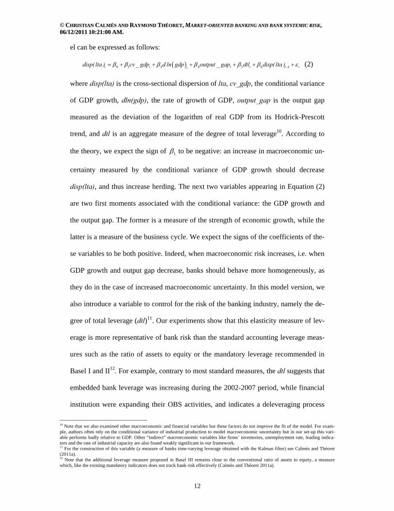
el can be expressed as follows:
0 1 3 4 5 6 1t t t t t ttdisp( lta ) cv _ gdp d ln gdp output _ gap dtl disp( lta ) (2)
where disp(lta) is the cross-sectional dispersion of lta, cv_gdp, the conditional variance
of GDP growth, dln(gdp), the rate of growth of GDP, output_gap is the output gap
measured as the deviation of the logarithm of real GDP from its Hodrick-Prescott
trend, and dtl is an aggregate measure of the degree of total leverage10. According to
the theory, we expect the sign of 1 to be negative: an increase in macroeconomic un-
certainty measured by the conditional variance of GDP growth should decrease
disp(lta), and thus increase herding. The next two variables appearing in Equation (2)
are two first moments associated with the conditional variance: the GDP growth and
the output gap. The former is a measure of the strength of economic growth, while the
latter is a measure of the business cycle. We expect the signs of the coefficients of the-
se variables to be both positive. Indeed, when macroeconomic risk increases, i.e. when
GDP growth and output gap decrease, banks should behave more homogeneously, as
they do in the case of increased macroeconomic uncertainty. In this model version, we
also introduce a variable to control for the risk of the banking industry, namely the de-
gree of total leverage (dtl)11. Our experiments show that this elasticity measure of lev-
erage is more representative of bank risk than the standard accounting leverage meas-
ures such as the ratio of assets to equity or the mandatory leverage recommended in
Basel I and II12. For example, contrary to most standard measures, the dtl suggests that
embedded bank leverage was increasing during the 2002-2007 period, while financial
institution were expanding their OBS activities, and indicates a deleveraging process
10 Note that we also examined other macroeconomic and financial variables but these factors do not improve the fit of the model. For exam-ple, authors often rely on the conditional variance of industrial production to model macroeconomic uncertainty but in our set-up this vari-able performs badly relative to GDP. Other “indirect” macroeconomic variables like firms’ inventories, unemployment rate, leading indica-tors and the rate of industrial capacity are also found weakly significant in our framework. 11 For the construction of this variable (a measure of banks time-varying leverage obtained with the Kalman filter) see Calmès and Théoret (2011a). 12 Note that the additional leverage measure proposed in Basel III remains close to the conventional ratio of assets to equity, a measure which, like the existing mandatory indicators does not track bank risk effectively (Calmès and Théoret 2011a).

© CCHHRRIISSTTIIAANN CCAALLMMÈÈSS AANNDD RRAAYYMMOONNDD TTHHÉÉOORREETT,, MMAARRKKEETT--OORRIIEENNTTEEDD BBAANNKKIINNGG AANNDD BBAANNKK SSYYSSTTEEMMIICC RRIISSKK,, 0066//1122//22001111 1100::2211::0000 AAMM..
13
after 2007, as banks were decreasing their risk to recover. Ceteris paribus, to the extent
that the herd-like hypothesis has some support, 5 , the coefficient of dtl should be
negative, banks adopting a more homogenous behaviour in times of increasing risk.
In order to estimate disp(lta) with a smoothed version of the conditional variance
of the GDP growth, we also run Equation (2) using the weighted conditional variance
measure of GDP growth (cv_gdp_w)13, whereas, in the third version of our model, the
dispersion of lta is expressed in terms of inflation uncertainty and reads as follows:
0 1 2 3 4 5 6 1t t t t t t ttdisp( lta ) cv _ inf d ln gdp output _ gap inf dtl disp( lta ) (3)
where cv_inf is the conditional variance of inflation and inf, the inflation rate, is the
first moment associated with the conditional variance of inflation. Similar to the case
of the conditional variance of GDP growth, we expect a negative sign for 1 , the coef-
ficient associated with inflation uncertainty. We also expect the coefficient associated
with the inflation rate, 4 , to be negative since inflation distorts the signal given by rel-
ative prices (Beaudry et al. 2001).
We then perform the same three estimations for the cross-sectional dispersion of
snonin, i.e. the cross-sectional dispersion of the risky assets associated with OBS ac-
tivities.
2.3. The EGARCH estimation methods
To estimate the three versions of our canonical model, we choose to rely on an
EGARCH approach using standard tests (Franses and Van Dijk 2000) because, as the
literature suggests, the standard OLS estimation method does not properly treat the in-
novation conditional heteroskedasticity. Relatedly, relying on OLS delivers mild re-
sults, especially regarding the impact of the first moments of the macroeconomic vari-
13 See Appendix 2 for more details on the conditional variance constructs.
© CCHHRRIISSTTIIAANN CCAALLMMÈÈSS AANNDD RRAAYYMMOONNDD TTHHÉÉOORREETT,, MMAARRKKEETT--OORRIIEENNTTEEDD BBAANNKKIINNGG AANNDD BBAANNKK SSYYSSTTEEMMIICC RRIISSKK,, 0066//1122//22001111 1100::2211::0000 AAMM..
14
ables14. The choice of this EGARCH methodology is also motivated by the fact that
the standard GARCH (p,q) does not rigorously account for the asymmetries encoun-
tered in many times series. For instance, bad news ( 0t i ) have generally a bigger
impact (i.e. a leverage effect) on financial returns volatility than good news ( 0t i ),
and an unexpected drop in returns (bad news) tend to increase the volatility more than
an unexpected rise in returns (good news) of a similar magnitude (Black 1976). In this
respect, we suspect that imposing a symmetry constraint on the conditional variance of
past innovations might be too restrictive, and actually inappropriate. Consequently, to
account for the likely asymmetric impact of good news and bad news on the condi-
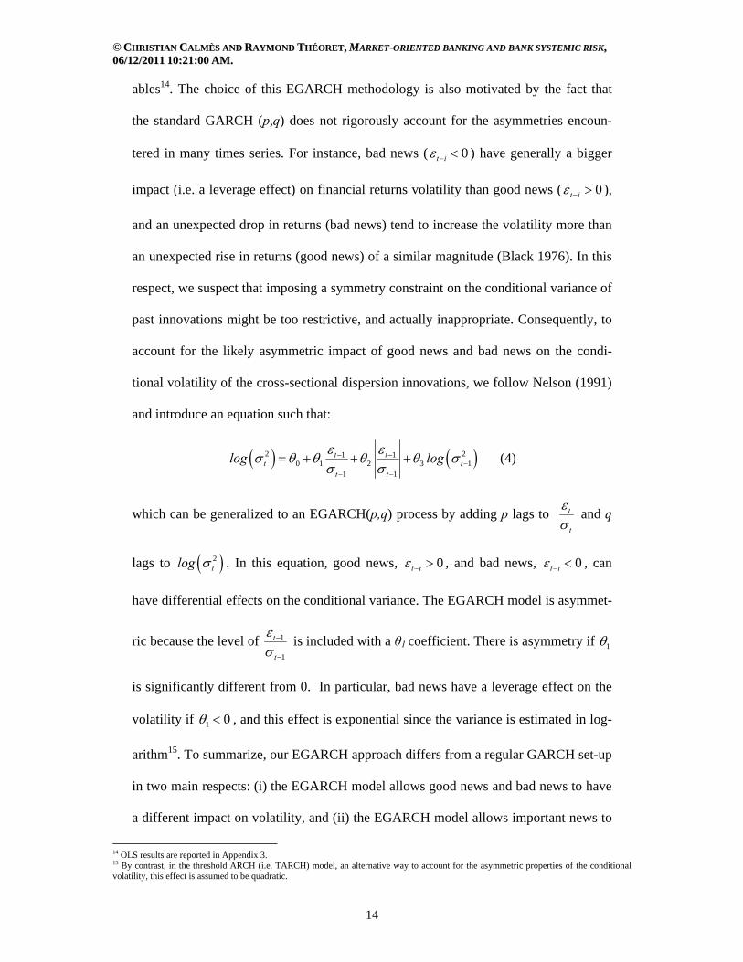
tional volatility of the cross-sectional dispersion innovations, we follow Nelson (1991)
and introduce an equation such that:
2 21 10 1 2 3 1
1 1
t tt t
t t
log log
(4)
which can be generalized to an EGARCH(p,q) process by adding p lags to t
t
and q
lags to 2tlog . In this equation, good news, 0t i , and bad news, 0t i , can
have differential effects on the conditional variance. The EGARCH model is asymmet-
ric because the level of 1
1
t
t
is included with a θ1 coefficient. There is asymmetry if 1
is significantly different from 0. In particular, bad news have a leverage effect on the
volatility if 1 0 , and this effect is exponential since the variance is estimated in log-
arithm15. To summarize, our EGARCH approach differs from a regular GARCH set-up
in two main respects: (i) the EGARCH model allows good news and bad news to have
a different impact on volatility, and (ii) the EGARCH model allows important news to
14 OLS results are reported in Appendix 3. 15 By contrast, in the threshold ARCH (i.e. TARCH) model, an alternative way to account for the asymmetric properties of the conditional volatility, this effect is assumed to be quadratic.

© CCHHRRIISSTTIIAANN CCAALLMMÈÈSS AANNDD RRAAYYMMOONNDD TTHHÉÉOORREETT,, MMAARRKKEETT--OORRIIEENNTTEEDD BBAANNKKIINNGG AANNDD BBAANNKK SSYYSSTTEEMMIICC RRIISSKK,, 0066//1122//22001111 1100::2211::0000 AAMM..
15
have a proportionally greater impact than the standard GARCH model (Engle and Ng
1993).
We estimate the model versions for lta and snonin using this EGARCH procedure,
but we also rely on EGARCH with instruments since the conditional variances of our
macroeconomic variables and the dtl series are generated variables, i.e. potentially
noisy proxies of their associated unobservable regressors (Pagan 1984, 1986). Indeed,
even if relying on OLS or simple maximum likelihood in the presence of generated
variables does not lead to inconsistency in the estimation procedure, the t tests associ-
ated with the estimated coefficients are however invalid (the F tests or Wald tests on
groups of coefficients still remaining valid, Pagan 1984, 1986). This issue is mentioned
in previous studies (e.g. Beaudry et al. 2001, Baum et al. 2002, 2004, 2009, Quaglia-
riello 2007, 2009) but, to our knowledge, it has not been fully addressed before. Ac-
cordingly, we adopt a comprehensive approach by first regressing the generated vari-
ables on instruments, including the predetermined variables, and also, as suggested by
Fuller (1987) and Lewbel (1997), the higher moments of the models explanatory vari-
ables. The second estimation method we use is thus a standard EGARCH with instru-
ments, or an IV-EGARCH, in which the generated variables cv_gdp, cv_gdp_w, cv_inf
and dtl are explicitly considered endogenous.
3. Data and some key stylized facts
In this paper we are not interested by extreme events such as liquidity crises. To
analyse crises episodes and the complete disruption of the banking system, authors
usually investigate the testable implications of the contagion theory, whereby a signal
triggers a bank run, in a cascade-herding traditional sense (Morris and Shin 2000, Lu-
cas and Stokey 2011). Since we focus instead on the regular reaction of the banking

© CCHHRRIISSTTIIAANN CCAALLMMÈÈSS AANNDD RRAAYYMMOONNDD TTHHÉÉOORREETT,, MMAARRKKEETT--OORRIIEENNTTEEDD BBAANNKKIINNGG AANNDD BBAANNKK SSYYSSTTEEMMIICC RRIISSKK,, 0066//1122//22001111 1100::2211::0000 AAMM..
16
system to the business cycle, it is desirable to rely on a dataset in which crises have a
relatively mild impact. In this respect, a Canadian sample appears to be one of the best
choices available. Indeed, as Bordo et al. (2011) argue, thanks to its domestic regula-
tion design, the Canadian banking system has been relatively immune to the subprime
crisis and to the former financial turmoils as well. Consequently, to better isolate the
impact of market-oriented banking on systemic risk, it is particularly instructive to
look at Canadian data. If we find that the changes in the banking environment have in-
deed some influence on banks usual response to macroeconomic shocks, then we
should expect that market-oriented banking has a fortiori significantly changed bank
risk in other countries, especially those which were the most hit by the recent crisis.
Accordingly, the sample we chose is derived from Canadian data and runs from
the first fiscal quarter of 1997 to the second fiscal quarter of 2010. We study the cross-
sectional dispersion of the risky assets of the six major Canadian banks on quarterly
data so that we have fifty-four observations, a reasonable number to perform standard
time series analysis. Our dataset is based on statistics provided by the Canadian Bank-
ers Association, the Office of the Superintendent of Financial Institutions, and the
Bank of Canada; and the macroeconomic time series come from CANSIM, a database
managed by Statistics Canada. Taken together, the six major domestic banks account
for about 90 percent of the banking business. All the banks we analyze are chartered
banks, i.e. commercial banks regulated by the Bank Act, running a broad range of ac-
tivities, from loan business to investment banking, fiduciary services, financial advice,
insurance and securitization.
Insert Figure 1 and Figure 2 here
Regarding the basic statistics, first note that the banks aggregate loans-to-assets ra-
tio displays a decreasing trend (Figure 1). In the first quarter of 1997 the lta ratio is
© CCHHRRIISSTTIIAANN CCAALLMMÈÈSS AANNDD RRAAYYMMOONNDD TTHHÉÉOORREETT,, MMAARRKKEETT--OORRIIEENNTTEEDD BBAANNKKIINNGG AANNDD BBAANNKK SSYYSSTTEEMMIICC RRIISSKK,, 0066//1122//22001111 1100::2211::0000 AAMM..
17
equal to 63%, but in the first quarter of 2010 it decreases to 54% after a low of 47% in
the second quarter of 2009 (at the peak of the subprime crisis). Relatedly, and opposite
to the lta pattern, snonin, our proxy for OBS activities has a tendency to increase over
the sample period (Figure 2). The ratio is equal to 43% at the beginning of the period
but in the third quarter of 2007 it rises to 55%. This new trend in banking has first been
identified by Boyd and Gertler (1994) for the U.S., and then further analyzed for many
countries, including in the now famous Rajan’s papers (2005, 2006)16. The literature
suggests that pari passu with the development of this market-oriented trend bank risk
has increased (e.g., Stiroh 2004, Stiroh and Rumble 2006, Baele et al. 2007, Wagner
2007, 2008 and 2010, Lepetit et al. 2008, Shin 2009). More precisely, authors find
that non-traditional business lines have spurred the volatility of bank income over the
last decades. Relatedly, it is also widely believed that bank risk is increasingly associ-
ated with the growth in off-balance-sheet activities, (Adrian and Shin 2009, Calmès
and Théoret 2010, Cardone et al. 2010, Nijkens and Wagner 2011).
Insert Figure 3 here
In this context, the question is then to assess the kind of impact this change in
banking has on systemic behaviour. In this respect, Figure 3 provides a first evidence,
showing the behaviour of the cross-sectional dispersions of the loans-to-assets ratio,
disp(lta), and of the share of noninterest income in operating revenues, disp(snonin),
from the first fiscal quarter of 1997 to the second fiscal quarter of 2010. The time se-
ries are obtained by computing the cross-sectional variances of the loans-to-assets ratio
(lta) and of the share of noninterest income (snonin) over the six banks for every quar-
ter. According to the evolution of the cross-sectional dispersion of lta, banks seem to
display an increase in herd-like behaviour over the period 1997-2002, but the trend
steadely reverses after 2002 (Figure 3). Surprisingly, this disp(lta) upward trend actu- 16 For Canadian evidence see also Calmès (2004).
© CCHHRRIISSTTIIAANN CCAALLMMÈÈSS AANNDD RRAAYYMMOONNDD TTHHÉÉOORREETT,, MMAARRKKEETT--OORRIIEENNTTEEDD BBAANNKKIINNGG AANNDD BBAANNKK SSYYSSTTEEMMIICC RRIISSKK,, 0066//1122//22001111 1100::2211::0000 AAMM..
18
ally persists, even during the last crisis. This constitutes preliminary evidence that the
banks traditional business has in fact become increasingly resilient, i.e. better immune
to external shocks. On other respect, a first glance at the series also reveals that the
cross-sectional dispersion of lta might be sensitive to the output gap. More precisely,
the cross-sectional dispersion of lta seems positively correlated with the output gap,
and this could suggest a priori more herd-like behaviour in bad times than in good
times. Note that this observation is not merely anecdotical since this kind of pattern is
much susceptible to increase banking procyclicality (Figure 3).
More importantly, note that, compared to what obtains with lta, the trend of the
cross-sectional dispersion of snonin is less pronounced over the whole sample period,
and strikingly drops after 2007, suggesting more herd-like behaviour in terms of non-
traditional activities. This volatility pattern is consistent with the studies arguing that
financial innovations tend to increase herding (e.g. Heiss 2005, Wagner 2008, Naka-
gawa and Uchida 2011). Relatedly, the cross-sectional dispersion of snonin appears to
be both more volatile and sensitive to the business cycle than the dispersion of lta, es-
pecially during recessions, when the banking system is the least resilient. For example,
during the last subprime crisis, a significant portion of securitized assets flowed back
on balance sheets and most of the credit commitments were also exercised. This kind
of response suggests that banks OBS activities might contract more than traditional
business lines during bad times. Finally, one curious pattern which seems to emerge
from Figure 3 is that the drops in the cross-sectional dispersion of snonin could pre-
date economic downturns17.
Insert Figure 4 and Figure 5 here
Another way of directly detecting herd-like behaviour is to examine the cyclical
17 That might be due to the fact that noninterest income is much related to stock market indices, which lead economic activity (Calmès and Théoret 2011b).

© CCHHRRIISSTTIIAANN CCAALLMMÈÈSS AANNDD RRAAYYMMOONNDD TTHHÉÉOORREETT,, MMAARRKKEETT--OORRIIEENNTTEEDD BBAANNKKIINNGG AANNDD BBAANNKK SSYYSSTTEEMMIICC RRIISSKK,, 0066//1122//22001111 1100::2211::0000 AAMM..
19
profile of the variance of the banking variables at stake. If we find that the variances
move procyclically, this could constitute an additional evidence of a cyclical conver-
gence in banking practices. Figures 4 and 5 provide the moving average variances of
the level and logarithm of banks loans and noninterest income, respectively. In these
figures we also plot as a benchmark the variances of the unscaled loans and noninterest
income variables. Captured this way, herding appears to be predominantly a cyclical
phenomenon, as there seems to be a regular decrease in the rolling variances of loans
and noninterest income, either prior or during contractions. Moreover, note that consis-
tent with the findings of Calmès and Liu (2009) and Calmès and Théoret (2010,
2011b), we can detect a regime change in loans and non-interest income volatility after
1996. Insofar as the variances of loans and noninterest income may be used as indica-
tors of banks systemic behaviour, data indicate a decrease in herding after 1997, the
volatilities of loans and noninterest income being much more pronounced after this
date. Actually, consistent with what Figure 3 suggests, since that date, economic
downturns seem to be preceded by variances surge.
4. Results
Table 1 provides the estimation results for the model versions based on the
EGARCH estimation without instruments. Columns (1) to (3) report the results of the
model estimation for the two dependent variables, the cross-sectional dispersions of lta
and snonin.
Insert Table 1 here
4.1. The lta and snonin cross-sectional dispersions
Column (1) of Table 1 displays the estimation results for Equation (2) and con-
firms that the increase in macroeconomic uncertainty lowers the cross-sectional disper-
© CCHHRRIISSTTIIAANN CCAALLMMÈÈSS AANNDD RRAAYYMMOONNDD TTHHÉÉOORREETT,, MMAARRKKEETT--OORRIIEENNTTEEDD BBAANNKKIINNGG AANNDD BBAANNKK SSYYSSTTEEMMIICC RRIISSKK,, 0066//1122//22001111 1100::2211::0000 AAMM..
20
sion of the loans-to-assets ratio, disp(lta). The estimated coefficient of cv_gdp is equal
to -0.79 and significant at the 1% level, and the coefficient of the weighted conditional
variance of GDP growth, cv_gdp_w, is even greater in absolute value, at -2.65, and
significant at the 5% level (Column (2)), a result which suggests a delay in the ad-
justement of disp(lta) to macroeconomic uncertainty.
Note that the level of economic growth also increases disp(lta), confirming that
banks systemic behaviour is more homogenous in economic downturns. Furthermore,
the estimated coefficient of dln(gdp) is equal to 0.83 and significant at the 10% level,
while the coefficient of output_gap is equal to 91.73 and significant at the 1% level.
According to these results, the first moments seem to play a greater role on herding
than reported in previous studies. Indeed, Quagliariello (2009) finds that the control
variables accounting for aggregate economic activity or inflation (i.e. first moments)
do not have a significant impact on the cross-sectional variability of the share that
banks invest in risky loans. Similarly, in Baum et al. (2002, 2004), the control vari-
ables also play a minor role in the OLS estimations. In this respect, the new results we
derive from our framework differ. One plausible reason explaining why the first mo-
ments are more significant in our case relates to the homoskedaticy hypothesis embed-
ded in previous studies. Indeed, to our knowledge, the conditional variance of the
equation innovations has never been explicitly specified before.
Equation (2) also delivers interesting results on clustering patterns when consider-
ing bank risk, as measured with our indicator of bank degree of total leverage, dtl. As
expected, column (1) of Table 1 shows that an increase in dtl decreases disp(lta), the
estimated coefficient being equal to -5.10 and significant at the 1% level. This result
supports the view that banks behaviour is more homogenous when bank risk increases,
and it is also broadly consistent with the impact of increases in macroeconomic risk
© CCHHRRIISSTTIIAANN CCAALLMMÈÈSS AANNDD RRAAYYMMOONNDD TTHHÉÉOORREETT,, MMAARRKKEETT--OORRIIEENNTTEEDD BBAANNKKIINNGG AANNDD BBAANNKK SSYYSSTTEEMMIICC RRIISSKK,, 0066//1122//22001111 1100::2211::0000 AAMM..
21
and uncertainty on disp(lta)18. With a coefficient of the lagged dependent variable at
0.59, and significant at the 1% level, column (1) also reveals that herd-like behaviour
is a persistent phenomenon (Haiss 2005, Nakagawa and Uchida 2011). One explana-
tion sometimes evoked in the literature relates to the Abilene paradox (Harvey 1974), a
kind of “mimetic isomorphism”, i.e. groupthink strategy characterized by copycat
banking practices.
Column (3) of Table 1 reports the corresponding results for Equation (3), the mod-
el including inflation as the proxy for macroeconomic uncertainty. Consistent with our
hypothesis of a negative link between the dispersion of the risky assets and uncer-
tainty, the estimated coefficient of cv_inf is negative, at -10.97 and significant at the
1% level. Inflation has also the expected negative impact on disp(lta), its estimated co-
efficient being equal to -1.27 and significant at the 5% level. These results support the
argument of Beaudry et al. (2001) and the idea that inflation generates noisy market
signals and increases clustering. In other respects, considering inflation instead of GDP
growth does not qualitatively alter the role played by economic growth. In particular,
the coefficient of dln(gdp) nearly doubles from 0.83 to 1.65 between the two specifica-
tions, and the coefficient of the output gap is also positive, at 60.40, and significant at
the 1% level.
Regarding market-oriented activities, given that they also relate to risky invest-
ments, we should anticipate that banks behave vis-à-vis snonin in the same way they
do with traditional activities. Table 1 largely qualifies this expectation. In particular,
economic uncertainty, as measured with the conditional variance of GDP (or inflation)
decreases disp(snonin). For example, the coefficient of cv_gdp is estimated at -1.09
and significant at the 1% level. More importantly, note that weighting the conditional
18 If, instead of dtl, we use a conventional measure of leverage like the ratio of assets to equity, the estimated coefficient is also nega-tive, although not significant at the usual thresholds.

© CCHHRRIISSTTIIAANN CCAALLMMÈÈSS AANNDD RRAAYYMMOONNDD TTHHÉÉOORREETT,, MMAARRKKEETT--OORRIIEENNTTEEDD BBAANNKKIINNGG AANNDD BBAANNKK SSYYSSTTEEMMIICC RRIISSKK,, 0066//1122//22001111 1100::2211::0000 AAMM..
22
variance of GDP growth does not improve the results in this case, the estimated coeffi-
cient of cv_gdp_w being equal to -2.07, but only significant at the 10% level (col-
umn(2)). Relatedly, when cv_gdp is used as the uncertainty proxy, the estimated coef-
ficient of the lagged dependent variable is equal to 0.18, a lower level than the corre-
sponding 0.59 obtained for disp(lta). This set of results suggests that disp(snonin) is
less persistent than disp(lta), a phenomenon which can be explained by the faster reac-
tion of OBS activities to economic activity and macroeconomic uncertainty. This dy-
namic property is consistent with both the relative volatility of snonin cross-sectional
dispersion, and the greater liquidity of non-traditional activities. For instance, loans
which are securitized generally display a high degree of liquidity, and their adjustment
to the desired value is thus arguably faster than for their on-balance-sheet counterparts.
Quite strikingly, note that disp(snonin) appears much more sensitive to inflation
uncertainty than lta. As a matter of fact, the coefficient of cv_inf is estimated at -49.20
and significant at the 1% level, while the corresponding coefficient for disp(lta) is
equal to -10.97 and significant at the 5% level19 (column (3)). Furthermore, and, again,
much more so than for disp(lta), economic growth significantly increases disp(snonin),
regardless of the macroeconomic factor proxying for uncertainty. For instance, with
the conditional variance of GDP growth, the estimated coefficient of the output gap is
equal to 287.26 and significant at the 1% level, whereas the corresponding coefficient
for disp(lta), at 91.73, is much lower (column(1)). In fact, for all the exogenous vari-
able considered, both those related to risk and to uncertainty, the results confirm our
stylized facts, namely the fact that the herding associated with non-traditional activities
appears more sensitive to macroeconomic shocks than it is the case for disp(lta). Re-
mark that these findings cannot obtain with the usual OLS approach, but our EGARCH
19 Note that the coefficients of the disp(lta) and disp(snonin) equations are directly comparable for a given explanatory variable since the ratios used to compute the cross-sectional dispersions are both defined on the [0,1] interval.
© CCHHRRIISSTTIIAANN CCAALLMMÈÈSS AANNDD RRAAYYMMOONNDD TTHHÉÉOORREETT,, MMAARRKKEETT--OORRIIEENNTTEEDD BBAANNKKIINNGG AANNDD BBAANNKK SSYYSSTTEEMMIICC RRIISSKK,, 0066//1122//22001111 1100::2211::0000 AAMM..
23
estimations clearly reveal that, while banks seem able to deal with the external shocks
hitting their loan business, at the same time, their non-traditional activities appear to be
both quite volatile and sensitive to the business cycle20.
Interestingly, the behaviours of disp(lta) and disp(snonin) also differ with respect
to dtl, our control variable for bank risk. Contrary to the disp(lta) results, an increase in
dtl leads to a corresponding increase in disp(snonin). The estimated coefficient of dtl is
positive and significant at the 1% level, regardless of the way we proxy for macroeco-
nomic uncertainty. For instance, it is equal to 18.86 when cv_gdp is used to measure
uncertainty, and to 23.82 with cv_inf. Relatedly, dtl and snonin positively comove and
an increase in snonin corresponds to an increase in risk as measured by dtl (Calmès
and Théoret 2011a). Furthermore, according to the data, when snonin increases,
disp(snonin) also tends to increase. This might actually explain the positive comove-
ment observed between dtl and disp(snonin). When dtl increases, banks have a ten-
dency to decrease their lta ratio, but not necessarily their OBS activities. Authors usu-
ally resort to a regulatory capital arbitrage (RCA) argument to explain this opposite re-
action to leverage (Jones 2000, Calomiris and Mason 2004, Ambrose et al. 2005, Kling
2009, Brunnermeier 2009, Cardone et al. 2010, Blundell-Wignall and Atkinson, Vives
2010). When dtl increases, i.e. bank risk rises, it may be due to an increase in snonin or
a decrease in bank liquidity ratio but, in any case, banks are induced to off-load risk
from on-balance-sheet to off-balance-sheet in order to generate new capital or addi-
tional liquidities21. Ceteris paribus, this transfer tends to decrease disp(lta) and lta, and
to increase disp(snonin) and snonin.
Insert Table 2 about here
To compare more precisely the relative power of our exogenous factors, Table 2
20 This observation nicely complements the seminal view that advances in risk management have essentially led to greater credit availability rather than reduced banking riskiness (Cebenoyan and Strahan 2004, Instefjord 2005). 21 For instance, some loans in the balance sheet may be securitized.

© CCHHRRIISSTTIIAANN CCAALLMMÈÈSS AANNDD RRAAYYMMOONNDD TTHHÉÉOORREETT,, MMAARRKKEETT--OORRIIEENNTTEEDD BBAANNKKIINNGG AANNDD BBAANNKK SSYYSSTTEEMMIICC RRIISSKK,, 0066//1122//22001111 1100::2211::0000 AAMM..
24
reports the estimated short-term and long-term elasticities of disp(lta) and
disp(snonin)22. When using cv_gdp_w as the uncertainty proxy, the elasticity of
disp(lta) is equal to -0.12 in the short-run, but more than doubles in the long-run, at
-0.29, a result in line with other studies (Baum et al. 2002, 2004, 2009). This confirms
that even if banks can adopt different strategies in the way they manage their tradi-
tional portfolio, they consistently tend to follow the same kind of adjustment to deal
with macroeconomic shocks. By comparison, the elasticity of disp(snonin) to GDP un-
certainty is lower, at -0.04 in the short-run and -0.05 in the long-run. This result sug-
gests that, as expected, banks herd-like behaviour is relatively more sensitive to uncer-
tainty when monitored with loans than with OBS activities. Indeed, as mentioned ear-
lier, the latter should be relatively more immune to uncertainty than risk since the vola-
tility of OBS activities is, by definition, easier to hedge. More importantly however,
these elasticities also confirm that market-oriented banking is particularly sensitive to
macroeconomic risk relative to traditional banking, a phenomenon which should de-
serve serious attention in the conduct of macroprudential policy.
Relatedly, our elasticity computations suggest that, consistent with Beaudry et al.
(2001) intuition, market-oriented activities are much influenced by inflation uncer-
tainty, likely because of the close negative link between inflation and stock markets
performance (Calmès and Théoret 2011b). In other words, ceteris paribus, when faced
with heightened inflation uncertainty, banks also tend to herd more in terms of non-
traditional business lines than with their loan portfolios. Note also that the long-run
elasticity of disp(lta) with respect to dtl, at -1.12, is higher than 1 in absolute value,
whereas the long-run elasticity of disp(snonin) with respect to dtl is also quite high, at
22 The elasticity of Y vis-à-vis X is computed using the following formula:
Xcoef
Y , where coef is the estimated coefficient of X, and X
and Y are respectively the average of Xt and Yt computed over the sample period. The long-term elasticity is computed by multiplying the
short-term elasticity by 1
1 , where is the coefficient of the lagged dependent variable.

© CCHHRRIISSTTIIAANN CCAALLMMÈÈSS AANNDD RRAAYYMMOONNDD TTHHÉÉOORREETT,, MMAARRKKEETT--OORRIIEENNTTEEDD BBAANNKKIINNGG AANNDD BBAANNKK SSYYSSTTEEMMIICC RRIISSKK,, 0066//1122//22001111 1100::2211::0000 AAMM..
25
0.87, but with the opposite sign. This finding clearly confirms that the positive impact
of a 1% increase of dtl on disp(snonin) is in fact mostly counterbalanced by the nega-
tive influence of this increase on disp(lta). As a consequence, we should conclude that
RCA unlikely exerts a meaningful influence on banks clustering in the long-run, or, to
be more exact, that regulatory regime changes have only weakly persistent effects on
banks systemic risk.
4.2. The volatility of the cross-sectional dispersions
The bottom of Table 1 reports the estimation results of the EGARCH processes
followed by the residuals of our dependent variables (Equation(4)). To our knowledge,
this modelization is a novelty in the literature. We experimented with several GARCH
processes and selected the EGARCH given its superior fit in terms of the usual tests.
Globally, our results indicate that omitting to specify the innovation volatility indeed
provides weaker fits23. The omission of the residuals specification in the studies based
on OLS, GARCH and GMM estimations might actually explain why authors often find
no significant role for the first moments of the explanatory variables (i.e. macroeco-
nomic risk).
Regarding the results, first note that, for disp(lta), the estimated asymmetry coeffi-
cient 1 of the EGARCH(1,1) is close to 1 and significant at the usual levels, regard-
less of the macroeconomic uncertainty factor considered (Table 1). In other words,
good news24 have a positive leverage effect on disp(lta) volatility, so the volatility of
disp(lta) is actually greater when disp(lta) increases. We observe the same phenome-
non with disp(snonin). In fact, the asymmetry coefficient is close to one for all the un-
23 The OLS estimations are discussed in Appendix 3. 24 Note that news are considered good or bad according to the sign of the innovation. We refer to good news when the innovation of disp(lta) is positive and to bad news when the innovation is negative. Indeed, our results indicate that disp(lta) increases with good news, as measured by the output gap or the GDP rate of growth.
© CCHHRRIISSTTIIAANN CCAALLMMÈÈSS AANNDD RRAAYYMMOONNDD TTHHÉÉOORREETT,, MMAARRKKEETT--OORRIIEENNTTEEDD BBAANNKKIINNGG AANNDD BBAANNKK SSYYSSTTEEMMIICC RRIISSKK,, 0066//1122//22001111 1100::2211::0000 AAMM..
26
certainty factors we consider. In this sense, our results are coherent in terms of the es-
timated volatilities of disp(lta) and disp(snonin). There is a significant asymmetry in
the volatility processes of these two variables, this asymmetry is both positive and
high, and it is robust to the various exogenous factors examined. Note that, since in
economic downturns, the volatilities of disp(lta) and disp(snonin) shrink pari passu
with the dispersions, these results lead us to conclude that the procyclicality of
disp(lta) and disp(snonin) might actually be greater than previously reported.
5. Robustness checks and complementary results
5.1. The IV-EGARCH estimation results
In our framework, we introduce as generated or endogenous variables a measure of
bank risk, dtl, and the conditional variances of the two macroeconomic variables we
use to define macroeconomic uncertainty. To tackle the econometric difficulty posed
by this kind of generated variables, we regress each of them on instruments before ap-
plying the EGARCH to the models. However doing so leaves our results essentially
unchanged. In particular, the results of the IV-EGARCH estimations show that, in the
regressions with disp(lta) as the dependent variable, the impact of cd_gdp and
cv_gdp_w decreases somewhat but remains significant at the 1% level (Table 3). How-
ever, the sensitivity of disp(lta) to cv_inf, even if it remains negative, is no longer sig-
nificant when using instruments. Without instruments, the coefficient of cv_inf is equal
to -10.97 and significant at the 5% level, while with the IV-EGARCH the coefficient is
equal to -3.55 and is no longer significant at the usual thresholds. This suggests that,
for disp(lta), the macroeconomic uncertainty measured with the growth of GDP might
be a more appropriate variable than the inflation proxy25.
25 This might also relate to the stabilization role played by the explicit inflation target adopted by the Canadian central bank.
© CCHHRRIISSTTIIAANN CCAALLMMÈÈSS AANNDD RRAAYYMMOONNDD TTHHÉÉOORREETT,, MMAARRKKEETT--OORRIIEENNTTEEDD BBAANNKKIINNGG AANNDD BBAANNKK SSYYSSTTEEMMIICC RRIISSKK,, 0066//1122//22001111 1100::2211::0000 AAMM..
27
By contrast, consistent with Beaudry et al. (2001) argument, the IV-EGARCH
confirms that disp(snonin) is quite sensitive to inflation uncertainty. Indeed, the impact
of cv_inf on disp(snonin) decreases somewhat from -49.20 to -27.44 with the IV-
EGARCH, but it remains significant at the 5% level, contrary to what obtains with
disp(lta) (Table 3).
Insert Table 3 about here
5.2. The cross-sectional covariances
Previous studies often consider that the risky assets cross-sectional dispersions
completely characterize banks comovements. Authors also assume that when disper-
sion decreases, banks herd-like behaviour necessarily accentuates. However, in some
situations this hypothesis might be misleading, and it could be necessary to look at
complementary statistics. In this respect, one additional indicator useful to monitor
bank systemic patterns is the assets cross-sectional covariance (Adrian 2007). This fi-
nancial indicator is defined as: 21 1
1 N N
i , j i ji j , j i
cov( X ) X X X XN N
, where
N is the number of banks analyzed, Xi is the risky asset to total assets ratio (lta or
snonin) of bank i, and X is the cross-sectional mean of X computed over the banks.
This statistics indicates the extent to which the (Xi, Xj) pairs comove in each time pe-
riod.
Insert Figure 6 here
Data show that, over the whole 1997-2010 period, the correlation between disp(lta)
and cov(lta) is equal to -0.55, and the correlation between disp(snonin) and
cov(snonin) is higher, at -0.91. Both statistics are significant at the 1% level. The
cross-sectional dispersions of lta and snonin thus seem a priori to be both coherent in-
© CCHHRRIISSTTIIAANN CCAALLMMÈÈSS AANNDD RRAAYYMMOONNDD TTHHÉÉOORREETT,, MMAARRKKEETT--OORRIIEENNTTEEDD BBAANNKKIINNGG AANNDD BBAANNKK SSYYSSTTEEMMIICC RRIISSKK,, 0066//1122//22001111 1100::2211::0000 AAMM..
28
dicators of the lta and snonin respective covariances (comovements). To illustrate the
relationship between the cross-sectional dispersions and covariances, Figure 6 provides
the scatter diagrams of disp(lta) and disp(snonin) with their respective cross-sectional
covariance. The negative colinearity between disp(lta) and cov(lta) appears quite high,
except for high values of disp(lta) for which the relationship deteriorates. According to
the dated dots of the scatter diagram, these extreme values are mostly associated with
the subprime crisis of 2007-2009 and its aftermath. The cross-sectional covariance of
lta increases from the third quarter of 2009 to the second quarter of 2010, while the
corresponding cross-sectional dispersion is at historical highs. This suggests that the
cross-sectional dispersion is actually an incomplete indicator of the comovement of
banks lta ratios during this kind of extreme episodes. Consistent with the correlations,
for snonin the observation dots relating the cross-sectional covariances to the cross-
sectional dispersions are more aligned with the regression line. However, there is also
a deterioration in the year 2008, and a closer look at the scatter diagram reveals that the
relationship between disp(snonin) and cov(snonin) might have shifted somewhat dur-
ing the crisis, as the comovements are accompanied by larger dispersions. Summariz-
ing, the cross-sectional dispersions of lta and snonin are generally realiable indicators,
but they may nevertheless be insufficient when the cross-sectional covariances are ig-
nored, especially so for contraction episodes.
Since herd-like behaviour is arguably more pronounced in downturns, the addi-
tional information conveyed by these cross-sectional covariances can prove to be a
useful complement to track bank systemic patterns. In particular, we can suspect that if
a cross-sectional covariance diverges from its associated cross-sectional dispersion,
this might signal a stronger banking resilience. In this respect, one way to interpret the
snonin scatter diagram, considering the strong alignment of the cross-sectional disper-

© CCHHRRIISSTTIIAANN CCAALLMMÈÈSS AANNDD RRAAYYMMOONNDD TTHHÉÉOORREETT,, MMAARRKKEETT--OORRIIEENNTTEEDD BBAANNKKIINNGG AANNDD BBAANNKK SSYYSSTTEEMMIICC RRIISSKK,, 0066//1122//22001111 1100::2211::0000 AAMM..
29
sion and covariance of the series, is that, on this dimension, the pattern again suggests
more herding vis-à-vis non-traditional activities. This final result is consistent with the
view that, in the new banking era, systemic risk might stem more from market-oriented
activities than from traditional business lines.
6. Conclusion Previous studies on bank risk have focused on traditional activities, essentially
lending. In this article we enlarge the analysis by integrating market-oriented banking
activities, which have now become a major source of bank income. The results we ob-
tain are robust to the addition of banks new business lines. In particular, when con-
fronted to increased macroeconomic uncertainty, banks adopt a more homogenous be-
haviour vis-à-vis both their traditional and market-oriented activities. Baum et al.
(2002, 2004) show that banks collective behaviour with respect to their risky assets is
robust to the composition of loans portfolios, and not a result specific to aggregate
loans26. We show that this pattern also obtains for assets whose cash-flows are nonin-
terest income. What we find is that banks herd-like behaviour is mostly observed in
contraction periods for both risky assets. In these episodes, the first and second mo-
ments associated with GDP growth play a similar role, and accentuate banks collective
appetite, away from risky assets, i.e. loans and OBS activities, and towards liquidity.
More precisely, in contractions, the output gap (i.e. first moment) decreases, the vola-
tility of GDP growth (second moment) increases, and both variables decrease the
cross-sectional dispersions of lta and snonin.
26 Baum et al. (2002, 2004) analyze aggregate loans and their components, i.e. three types of risky assets, namely real estate loans, household loans, and commercial and industrial loans. The authors find that bank clustering prevails not only for aggregate loans but also for these components. Their results are particularly prevalent for real estate loans, whose cross-sectional dispersion increases sharply over the period they analyze.
© CCHHRRIISSTTIIAANN CCAALLMMÈÈSS AANNDD RRAAYYMMOONNDD TTHHÉÉOORREETT,, MMAARRKKEETT--OORRIIEENNTTEEDD BBAANNKKIINNGG AANNDD BBAANNKK SSYYSSTTEEMMIICC RRIISSKK,, 0066//1122//22001111 1100::2211::0000 AAMM..
30
However, a comparison of lta and snonin statistics also reveals that herding might
be more prevalent for non-traditional activities, and thus that, ceteris paribus, banking
fragility could increasingly stem from market-oriented banking. In this respect, our
main results support the view that, in the new banking era, banking stability and sys-
temic risk are more related to OBS activities than to the traditional loan business lines.
In particular, in the context of shadow banking, the fact that the cross-sectional disper-
sion of snonin appears quite sensitive to economic downturns might be a new source of
concern for policy-makers. The assets involved in OBS activities, like securitized as-
sets, are more liquid than loans, and can flow back quickly on balance sheet, precipitat-
ing the decrease in these activities during contractions. We find that banks’ snonin ac-
tually tend to converge rapidly during contractions, which indeed implies major banks
portfolios reshufflings. The strong sensitivity to the business cycle phase (first mo-
ment) of the cross-sectional dispersion of snonin likely relates to first-order demand-
side effects emanating from the buyers of the short-term debts financing the securitized
assets, from the lenders of the repo market27, and from firms exercising massively their
credit commitments during contractions. For example, the buyers of the special in-
vestment vehicles (SIV) short-term debt can provoke a technical run in time of liquid-
ity shortage simply by not rolling over their investments (Vives 2010, Gennaioli et al.
2011). The sponsor banks are then simultaneously forced to recuperate the SIV’s assets
on their balance sheets, and securitization thus creates a strong correlation in the re-
turns of intermediaries in bad times. In the same vein, there can be a surge in firms’
bank credit commitments during expansions, but they have to be eventually followed
by a massive commitments exercise during contractions, a boomerang effect amplify-
ing the cyclicality of snonin cross-sectional dispersion. 27 The repo market induces banks to reshuffle their OBS activities in periods of contractions or liquidity shortages. According to Lucas and Stokey (2011), the repo market pools cash reserves, like other forms of fractional reserve banking. A pillar of market-based financing, this market shrinks heavily during contractions, and especially during liquidity crises, a phenomenon indirectly captured in our framework by the major decrease in the cross-sectional dispersion of snonin observed during financial turmoils.
© CCHHRRIISSTTIIAANN CCAALLMMÈÈSS AANNDD RRAAYYMMOONNDD TTHHÉÉOORREETT,, MMAARRKKEETT--OORRIIEENNTTEEDD BBAANNKKIINNGG AANNDD BBAANNKK SSYYSSTTEEMMIICC RRIISSKK,, 0066//1122//22001111 1100::2211::0000 AAMM..
31
These demand-side effects must be distinguished from the impact of macroeco-
nomic uncertainty (the second moment) on banks systemic behaviour. We find that the
dispersion of snonin seems relatively less sensitive to macroeconomic uncertainty than
the dispersion of lta. In this respect, while many studies indicate that the rising share of
OBS activities in banks total operations is associated with an increase in the volatility
of bank performance (Calmès and Théoret 2010, Uhde and Michalak 2010, Nijskens
and Wagner 2011, Sanya and Wolfe 2011), our results suggest that OBS activities
might also help banks hedge and better allocate their risks in the long-run (Stiroh
2004).
To the extent that the cyclical aspects of banks collective behaviour are related to
the efficiency and stability of the financial system, an important contribution of our
study is first to show that, despite the change in the banking landscape, banks herd-like
behaviour remains predominantly a cyclical phenomenon at long horizons, particularly
at play during economic contractions; and second that, nevertheless, shadow banking
might have changed the way banks manage risks. On the one hand, in the traditional
Baumol sense, market-oriented banking offers a more efficient management of liquid-
ity. With the development of shadow banking, liquidity management is more in sink
with leverage fluctuations, conventional liquidity ratios are strikingly lower, the ratio
of loans loss provisions seems also lower, while, concomitantly, banks effective lever-
age can increase. On the other hand however, this new banking landscape is also ac-
companied by increased strategic complementarities, higher risk and higher probabili-
ties of insolvency. In this respect, our study suggests that, far from having reduced
banking cyclicality, despite the greater risk-sharing embodied in non-traditional activi-
ties, the new business lines could actually increase the volatility of banks assets.

© CCHHRRIISSTTIIAANN CCAALLMMÈÈSS AANNDD RRAAYYMMOONNDD TTHHÉÉOORREETT,, MMAARRKKEETT--OORRIIEENNTTEEDD BBAANNKKIINNGG AANNDD BBAANNKK SSYYSSTTEEMMIICC RRIISSKK,, 0066//1122//22001111 1100::2211::0000 AAMM..
32
The main macroprudential policy implication we can derive from this study is that
the cyclicality of OBS activities should be closely monitored by the regulatory agen-
cies in charge of financial stability. The traditional role of banks, which consists in
providing liquidities sur demande to the economic system is obviously challenged by
the development of banks non-traditional activities, which melt conventional and in-
vestment banking. In particular, our study shows that, in this dimension, the banking
system is both volatile and exposed to the business cycle. Macroprudential policy-
makers face a delicate conundrum, as the increase in banking aggregate risk (relative
to idiosyncratic risk), one of the most singular characteristics of the new banking envi-
ronment28, is accompanied by a new concept of liquidity, not yet fully understood (Lu-
cas and Stokey 2011, Loutskina 2011). For example, when it comes to the Basle III
proposed mandatory leverage ratio, we would strongly advocate to envisage broader
definitions of leverage to fully capture the new liquidity management practices associ-
ated with market-oriented activities (Calmès and Théoret 2011a). This is left for future
work.
Appendix 1
The banks portfolio model
As usually assumed in the literature, the returns on the two categories of assets
which compose the representative bank portfolio are given by the following equations:
Si ,t fi, t , r r (5)
rai ,t f i ,ti, t , r r (6)
where Si ,tr is the return on the security for bank i at time t; fr is the return on a risk-free
28 Houston and Stiroh (2006) and Gennaioli et al. (2011) find that bank systemic risk increased with the development of shadow banking, while idiosyncratic risk decreased thanks to the greater diversification enabled by OBS activities.
© CCHHRRIISSTTIIAANN CCAALLMMÈÈSS AANNDD RRAAYYMMOONNDD TTHHÉÉOORREETT,, MMAARRKKEETT--OORRIIEENNTTEEDD BBAANNKKIINNGG AANNDD BBAANNKK SSYYSSTTEEMMIICC RRIISSKK,, 0066//1122//22001111 1100::2211::0000 AAMM..
33
asset and rai ,tr is the return on the risky asset. The expected return on the risky asset is
equal to fr , where is the expected risk premium assumed to be fixed. The idio-
syncratic risk is represented by the random variable ),0(~ 2,, tti N . At time t, when
bank i determines the optimal allocation of its portfolio between the security and the
risky asset, it is confronted to uncertainty, i ,t (Equation (6)). Assume that at time t
each bank i observes an imperfect signal i ,tS which enables the bank to formulate a
prediction on the value of i ,t : , ,i t i t tS , with ),0(~ 2,tt N and 0it tE , 29.
The assumption of orthogonality between it and t may be justified by considering t
as an aggregate shock uncorrelated to the idiosyncratic shock. At time t, each bank i
observes a different signal i ,tS comprising an heterogeneous shock i ,t and a homoge-
nous noise t whose intensity 2,t is time varying. We assume that 2
,t is driven by
macroeconomic uncertainty so that when uncertainty rises, the noise incorporated in
the signal rises with 2,t , and it becomes increasingly difficult to determine the true
value of i ,t and the optimal return on loans. The best way to predict the return on the
risky asset is then to estimate i ,t i ,tE | S , the expected value of the idiosyncratic noise
conditional on the signal. Even if i ,tE , the unconditional expectation of the idiosyn-
cratic noise, is equal to 0, this is not the case for its conditional counterpart. Consistent
with Baum et al. (2002, 2004) we thus assume that the conditional expectation of i ,t is
equal to a proportion t of the signal:
i ,t i ,t t i ,t ti, t , E | S (7)
with
29 For a canonical form of this banking theory based on signal extraction see Rajan (1994). Rajan relates the signal to the publication of banks earnings rather than macroeconomic time series, but there is obviously a close link between bank earnings and macroeconomic aggregates (Bikker and Hu 2002, Quagliariello 2008).
© CCHHRRIISSTTIIAANN CCAALLMMÈÈSS AANNDD RRAAYYMMOONNDD TTHHÉÉOORREETT,, MMAARRKKEETT--OORRIIEENNTTEEDD BBAANNKKIINNGG AANNDD BBAANNKK SSYYSSTTEEMMIICC RRIISSKK,, 0066//1122//22001111 1100::2211::0000 AAMM..
34
2
2 2,t
t,t ,t
t ,
(8)
We then compute itw , the optimal share of the risky asset in the bank portfolio.
The expected return of the portfolio conditional on the signal is equal to:
1i ,t i ,t i ,t f t i ,t i ,t fi, t , E R | S w r S w r
(9)
and the conditional variance of the portfolio is:
2 2i ,t i ,t t ,t i ,ti, t , Var R | S w
(10)
According to this straightforward model, the portfolio variance is simply an increasing
function of macroeconomic uncertainty 2,t . Banks maximize a standard utility func-
tion i ,tV which depends positively on the expected return of the portfolio, and nega-
tively on risk as measured by its variance,
1
2i ,t
i ,t i ,t i ,t i ,t i ,t i ,tw
i, t , arg max E V | S E R | S Var R | S
(11)
where is the bank degree of risk aversion. Equating the derivative of Equation (11)
with respect to wi,t to 0, we obtain the optimal value of the share of the risky asset in
the bank portfolio,
2t i ,t
i ,tt ,t
Si, t , w
(12)
Combining Equations (12) and (8) we can finally compute the variance of the cross-
sectional dispersion of the risky asset as follows:
2 2
2 4,t ,t
i ,t,t
i, t , Var w
(13)
Its derivative with respect to macroeconomic uncertainty 2,t is thus:
2
2 2 6 4
21 10i ,t ,t
,t ,t ,t
Var wi, t ,
(14)

© CCHHRRIISSTTIIAANN CCAALLMMÈÈSS AANNDD RRAAYYMMOONNDD TTHHÉÉOORREETT,, MMAARRKKEETT--OORRIIEENNTTEEDD BBAANNKKIINNGG AANNDD BBAANNKK SSYYSSTTEEMMIICC RRIISSKK,, 0066//1122//22001111 1100::2211::0000 AAMM..
35
Equation (14) is the herd-like hypothesis we examine in this study.

© CCHHRRIISSTTIIAANN CCAALLMMÈÈSS AANNDD RRAAYYMMOONNDD TTHHÉÉOORREETT,, MMAARRKKEETT--OORRIIEENNTTEEDD BBAANNKKIINNGG AANNDD BBAANNKK SSYYSSTTEEMMIICC RRIISSKK,, 0066//1122//22001111 1100::2211::0000 AAMM..
36
Appendix 2
The conditional variance constructs
In line with Baum et al. (2002, 2004, 2009) and Quagliariello (2007, 2009) we
model our conditional variances, i.e. the indicators of macroeconomic uncertainty, us-
ing GARCH (p,q) specifications (Bollerslev 1986). However, contrary to these au-
thors, we also introduce EGARCH specifications (Nelson 1991) to model macroeco-
nomic uncertainty and test the herd-like hypothesis. Assume a simple general econo-
metric model written as:
t t tY X (15)
with tY the vector of the dependent variable, tX the matrix of the explanatory vari-
ables, 2 0t t~ iid , the innovation, and 2t the conditional variance of the innova-
tion. This conditional variance follows a GARCH (1,1) process if it can be written as
follows:
2 2 21 1t t t (16)
which can be generalized to a GARCH (p,q) process by adding p lags to t and q lags
to 2t . Equations (15) and (16) are estimated simultaneously using the maximum like-
lihood estimator.
Then, to build the conditional variances of our two proxies of macroeconomic un-
certainty, respectively based on the GDP and the consumer price index, we first trans-
form these variables in growth rates so that we can work with stationary time series.
Otherwise, if the series were not transformed in quarterly percentage rate of changes,
the resulting conditional variances would be dominated by the trend of these variables.
Transforming the series this way enables us to capture the cyclical fluctuations of the
© CCHHRRIISSTTIIAANN CCAALLMMÈÈSS AANNDD RRAAYYMMOONNDD TTHHÉÉOORREETT,, MMAARRKKEETT--OORRIIEENNTTEEDD BBAANNKKIINNGG AANNDD BBAANNKK SSYYSSTTEEMMIICC RRIISSKK,, 0066//1122//22001111 1100::2211::0000 AAMM..
37
proxies.
Insert Table A2 here
The computations related to the conditional variables are provided in Table A2. To
construct the conditional variance of GDP growth, the measure of macroeconomic un-
certainty related to this variable, we first rely on an ARMA (2,2) specification to esti-
mate the GDP growth expected mean, selected on the basis of the usual Akaike and
Schwartz criteria. We then use an EGARCH (1,1) to compute the associated condi-
tional variance of GDP growth after experimenting with several GARCH processes30.
The estimations results are provided in Table A2. The estimated coefficient of asym-
metry 1 (Equation (4)) is negative, so bad news indeed seem to have a leverage effect
on the volatility of GDP growth. Since the resulting profile of the conditional volatility
of GDP growth is somewhat unstable, we also use a weighted variance of the current
and last three quarters’ conditional variances (cv_gdp_w), with arithmetic weights 0.4,
0.3, 0.2 and 0.1. Similarly, the conditional variance of inflation is computed with an
IGARCH(1,1)31 (integrated GARCH) resulting from an AR(1) estimation. The condi-
tional variance seems very persistent, the coefficient of 21t being estimated at 0.78.
30 For the tests related to the selection of a GARCH process, see Franses and van Dijk (2000). 31 In an IGARCH process the sum of the and coefficients in equation (16) is close to 1.
© CCHHRRIISSTTIIAANN CCAALLMMÈÈSS AANNDD RRAAYYMMOONNDD TTHHÉÉOORREETT,, MMAARRKKEETT--OORRIIEENNTTEEDD BBAANNKKIINNGG AANNDD BBAANNKK SSYYSSTTEEMMIICC RRIISSKK,, 0066//1122//22001111 1100::2211::0000 AAMM..
38
Appendix 3
OLS estimations of the cross-sectional dispersions of lta and snonin
Table A3 provides the OLS estimations of the cross-sectional dispersions of lta
and snonin over the period 1997-2010, the model specifications being the same as
those used for the EGARCH estimations (Table 1). As mentioned, the results are poor
compared to those obtained with our EGARCH procedure. In particular, the results as-
sociated with the OLS estimation of disp(lta) are clearly unsatisfactory. Indeed, the on-
ly variable which is significant at the 5% level across all the model specifications is the
rate of growth of GDP, which displays the same sign as in the EGARCH estimation.
The conditional variance of GDP (cv_gdp) has the expected negative sign but is not
significant, while the conditional variance of inflation (cv_inf) has the wrong sign, also
insignificant. Moreover, the output gap has a sign opposite to its EGARCH estimate,
although insignificant. The dtl variable has the same sign as in the EGARCH estima-
tion but is also not significant.
Insert Table A3 here
The results obtained with the OLS estimation of disp(snonin) are more in line with
those resulting from our EGARCH estimation. The variable cv_gdp has the expected
sign and is significant at the 10% level, while cv_inf has also the right sign and is sig-
nificant at the 5% level. Similarly, for disp(snonin), the variable dtl has the same sign
as in the EGARCH estimation in the model featuring cv_gdp as the indicator of mac-
roeconomic uncertainty, and is significant at the 10% level. Overall, the OLS estima-
tions confirm that the EGARCH results found for disp(snonin) are particularly robust
© CCHHRRIISSTTIIAANN CCAALLMMÈÈSS AANNDD RRAAYYMMOONNDD TTHHÉÉOORREETT,, MMAARRKKEETT--OORRIIEENNTTEEDD BBAANNKKIINNGG AANNDD BBAANNKK SSYYSSTTEEMMIICC RRIISSKK,, 0066//1122//22001111 1100::2211::0000 AAMM..
39
since they remain the same with a linear approach. In this case, the OLS results consti-
tute an additional evidence that banks market-oriented business lines are quite sensitive
to the business cycle. This observation suggests that herding seems indeed to be more
severe for market-oriented activities than for loans, a finding which underlines the fra-
gility to which new business lines expose the banking system.
Finally, note that the OLS estimations do not deliver significant results regarding
the impact of the marcoeconomic first moments. In this respect, the results we obtain
when modelling the innovation volatility are superior for both disp(lta) and
disp(snonin). In this respect, it appears quite important to model the conditional vola-
tility of the innovations of the cross-sectional dispersion equations as we do.
© CCHHRRIISSTTIIAANN CCAALLMMÈÈSS AANNDD RRAAYYMMOONNDD TTHHÉÉOORREETT,, MMAARRKKEETT--OORRIIEENNTTEEDD BBAANNKKIINNGG AANNDD BBAANNKK SSYYSSTTEEMMIICC RRIISSKK,, 0066//1122//22001111 1100::2211::0000 AAMM..
40
References Adrian, T., 2007. Measuring risk in the hedge fund sector. Current issues in Econom-
ics and Finance 13, 1-7. Adrian, T., Brunnermeier, M.K., 2008. CoVaR. Staff Report, Federal Reserve Bank of
New York. Adrian, T, Shin, H.S., 2009. The shadow banking system: Implications for financial
regulation. Staff Report, Federal Reserve Bank of New York. Ambrose, B.W., Lacour-Little, M, Sanders, A.B., 2005. Does regulatory capital arbi-
trage, reputation or asymetric information drive securitization? Journal of Financial Services Research 28, 113-133.
Baele, L., DeJonghe, O., Vennet, R.V., 2007. Does the stock market value bank diver-sification. Journal of Banking and Finance 31, 1999-2023.
Barrell, R., Davis, E.P., Karim D., Liadzze, I., 2010. Evaluating Off-balance sheet ex-posures in banking crisis determination models. Working paper, Brunel University.
Barth, J., R., Caprio, G., Levine, R., 1999. Financial regulation and performance: Cross-country evidence. Working paper 2037, World Bank.
Baum, C. F., Caglayan, M., Ozkan, N., 2002. The impact of macroeconomic uncer-tainty on bank lending behavior. Working Paper, University of Liverpool.
Baum, C. F., Caglayan, M., Ozkan, N., 2004. The second moment matters: the re-sponse of bank lending behavior to macroeconomic uncertainty. Working Paper, Boston College.
Baum, C. F., Caglayan, M., Ozkan, N., 2009. The second moment matters: the impact of macroeconomic uncertainty on the allocation of loanable funds. Economics Let-ters 102, 87-89.
Beaudry, P., Caglayan, M., Schiantarelli, F., 2001. Monetary instability, the predict-ability of prices, and the allocation of investment: An empirical investigation using panel data. American Economic Review 91, 648-662.
Bernanke, B, .S., Gertler, N., 1989. Agency cost, net worth, and business fluctuations. American Economic Review 79, 14-31.
Bernanke, B., S., Gertler, N., 1995. Inside the black box: the credit channel of mone-tary policy transmission. Journal of Economic Perspectives 9, 27-48.
Bikker, J.A., Hu, H. 2002. Cyclical patterns in profits, provisioning, and lending of banks and procyclicality of the new Basel capital requirements. Banca Nazionale del Lavoro Quarterly Review 55, 143-175.
Bikker, J.A., Metzemakers, P., A., J., 2005. Bank provisioning behavior and procycli-cality. Journal of International financial Markets, Institutions and Money 15, 141-157.
Black, F., 1976. Studies of stock price volatility of changes. American Statistical As-sociation Journal, 177-181.
Blundell-Wignall, A., Atkinson, P., 2010. Thinking beyond Basle III: Necessary solu-tions for capital and liquidity. Financial Markets Trends 20, 1-23.
Bollerslev, T., 1986. Generalized autoregressive conditional heteroskedasticity. Jour-nal of Econometrics 31, 307-328.
Bordo, M.D., Redish, A., Rockoff, H., 2011. Why didn’t Canada have a banking crisis in 2008 (or in 1930, or 1907, or...)? Working Paper, NBER.
Borio, C. Furfine, C., Lowe, P., 2001. Procyclicality of the financial system and finan-cial stability: issues and policy options. BIS paper 1-2001.
© CCHHRRIISSTTIIAANN CCAALLMMÈÈSS AANNDD RRAAYYMMOONNDD TTHHÉÉOORREETT,, MMAARRKKEETT--OORRIIEENNTTEEDD BBAANNKKIINNGG AANNDD BBAANNKK SSYYSSTTEEMMIICC RRIISSKK,, 0066//1122//22001111 1100::2211::0000 AAMM..
41
Boyd, J.H., Gertler, M., 1994. Are banks dead? Or are the reports greatly exaggerated? Federal Reserve Bank of Minneapolis Quarterly Review 18, 1-27.
Brunnermeier, M.K., 2009. Deciphering the liquidity and credit crunch 2007-2008. Journal of Economic Perspectives 23, 77–100.
Calmès, C., 2004. Regulatory changes and financial structure: The case of Canada. Swiss Journal of Economics and Statistics 140, 1-35.
Calmès, C., Liu, Y., 2009. Financial structure change and banking income: A Canada- U.S. comparison. Journal of International Financial Markets, Institutions and Money 19, 128-139.
Calmès, C., Théoret, R., 2010. The impact of off-balance-sheet activities on banks re-turns: An application of the ARCH-M to Canadian data. Journal of Banking and Finance 34(7), 1719-1728.
Calmès, C., Théoret, R., 2011a. Shadow banking and leverage: an application of the Kalman filter to time-varying cyclical leverage measures. Chaire d’information fi-nancière et organisationnelle ESG-UQAM Working paper 2011-01.
Calmès, C., Théoret, R., 2011b. The rise of shadow banking and the hidden benefits of diversification. Chaire d’information financière et organisationnelle ESG-UQAM Working paper 2011-02.
Calomiris, C.W., Mason, J.R., 2004. Credit card securitization and regulatory arbi-trage. Journal of Financial Services Research 26, 5-27.
Cardone Riportella, C, Samaniego Medina, R., Tujilo Ponce, A., 2010. What drives bank securitization? The Spanish experience. Journal of Banking and Finance, 34, 2639-2651.
Cebenoyan, A.S., Strahan, P.E., 2004. Risk management, capital structure and lending at banks. Journal of Banking and Finance 28, 19-43.
De Jonghe, O.G., 2010. Back to the basics in banking? A micro-analysis of banking system stability. Journal of Financial Intermediation 19, 387-417.
Diamond, D., Dybvig, P., 1983. Bank runs, deposit insurance, and liquidity. Journal of Political Economy 91, 401-419.
Engle, R.F., Ng, V.K., 1993. Measuring and testing the impact of news on volatility. Journal of Finance 48, 1749-1778.
Farhi, E., Tirole, J., 2009. Collective moral hazard, maturity mismatch and systemic bailouts. Working paper, NBER.
Franses, P.H., van Dijk, D., 2000. Non-Linear Time Series Models in Empirical Fi-nance. Cambridge University Press: Cambridge.
Fuller, W.A., 1987. Error Models, John Wiley & Sons. Gauthier, C., Lehar, A., and Souissi, M., 2010. Macroprudential Regulation and Sys-
temic Capital Requirements, Working Paper 2010-4, Bank of Canada. Gennaioli, N., Shleifer, A., Vishny, R.W., 2011. A model of shadow banking. Work-
ing paper, NBER. Haiss, P. R., 2005. Banks, herding and regulation: A review and synthesis. Working
paper, Europe Institute. Harvey, J., 1974. The Abilene paradox: the management of agreement. Organizational
Dynamics. Hirshleifer, D., Teoh, S., H., 2003. Herd behavior and cascading in capital markets: a
review and synthesis. European Financial Management 9, 25-66. Houston, J.F., and Stiroh, K.J., 2006. Three decades of financial sector risk. Staff Re-
port, Federal Reserve Bank of New York. Huizinga, J., 1993. Inflation, uncertainty, relative price uncertainty, and investment in
U.S. manufacturing. Journal of Money, Credit and Banking, 25 3, 521-549.
© CCHHRRIISSTTIIAANN CCAALLMMÈÈSS AANNDD RRAAYYMMOONNDD TTHHÉÉOORREETT,, MMAARRKKEETT--OORRIIEENNTTEEDD BBAANNKKIINNGG AANNDD BBAANNKK SSYYSSTTEEMMIICC RRIISSKK,, 0066//1122//22001111 1100::2211::0000 AAMM..
42
Hutchison, M., N., 2002. European banking distress and EMU: institutional and mac-roeconomic risk. Scandinavian Journal of Economics 104, 365-389.
Hyytinen, A., Kuosa, I., Takalo, T., 2003. Law or finance: evidence from Finland. Eu-ropean Journal of Law and Economics 16, 59-89.
Hwang, S., Salmon, M., 2004. Market stress and herding. Journal of Empirical Fi-nance 11, 585-616.
Instefjord, N., 2005. Risk and herding: Do credit derivatives increase bank risk? Jour-nal of Banking and Finance 29, 333-345.
Jain, A. K., Gupta, S., 1987. Some evidence on “herding” behavior of U.S. banks. Journal of Money Credit and Banking 19, 78-89.
Jones, D., 2000. Emerging problems with the Basel Capital Accords: Regulatory capi-tal arbitrage and related issues. Journal of Banking Finance 24, 35-58.
Kane, E., 1981. Impact of regulation on economic behavior: accelerating inflation, technological innovation, and the decreasing effectiveness of banking regulation. Journal of Finance 36, 355-367.
Kashyap, A.K., Stein, J.C., 2000. What do a million observations on banks say about the transmission of monetary policy. American Economic Review 90, 407-428.
Kling, A., 2009. Not what they had in mind: A history of policies that produced the fi-nancial crisis of 2008. Working paper, Mercatus Center, George Mason University.
Kyotaki, N., Moore, J., 1997. Credit cycles. Journal of Political Economy 105, 211-248.
Lepetit, L., Nys, E., Rous, P., Tazari, A., 2008. Bank income structure and risk : An empirical analysis of European banks. Journal of Banking and Finance 32, 1452-1467.
Lewbel A., 1997. Constructing instruments for regressions with measurement error when no additional data are available, with an application to patents and R&D. Econometrica 65, 1201-1213.
Llewellyn, D., 2002. An analysis of the causes of recent banking crises. European Journal of Finance 8, 152-175.
Loutskina, E., 2011. The role of securitization in bank liquidity and funding manage-ment. Journal of Financial Economics 100, 663-684.
Lucas, R. E. Jr., 1973. Some international evidence on output-inflation trade-offs. American Economic Review 63, 326-334.
Lucas, R.E. Jr., Stokey, N.L., 2011. Liquidity crises, understanding sources and limit-ing consequences: A theoretical framework. The Region, Federal Reserve Bank of Minneapolis, 1-11.
Martin, A., Parigi, B.M., 2011. Bank capital regulation and structured finance. Work-ing paper. Federal Reserve Bank of New York.
Morris, S., Shin, H.S., (2000). Rethinking multiple equilibria in macroeconomic mod-elling. NBER Macroeconomics Annual 15, 139-161.
Nakagawa, R., Uchida, H., 2011. Herd behaviour of Japanese banks after financial de-regulation. Economica (forthcoming).
Nelson, D.B., 1991. Conditional heteroskedasticity in asset returns: A new approach. Econometrica 59, 347-370.
Nijskens, R, Wagner, W., 2011. Credit risk transfer activities and systemic risk: How banks became less risky individually but posed greater risks to the financial system at the same time. Journal of Banking and Finance 35, 1391-1398.
Pagan, A.R., 1984. Econometric issues in the analysis of regressions with generated regressors. International Economic Review 25, 221-247.
Pagan, A.R., 1986. Two stage and related estimators and their applications. Review of

© CCHHRRIISSTTIIAANN CCAALLMMÈÈSS AANNDD RRAAYYMMOONNDD TTHHÉÉOORREETT,, MMAARRKKEETT--OORRIIEENNTTEEDD BBAANNKKIINNGG AANNDD BBAANNKK SSYYSSTTEEMMIICC RRIISSKK,, 0066//1122//22001111 1100::2211::0000 AAMM..
43
Economic Studies 53, 517-538. Pecchino, R., 1998. Risk averse bank managers: exogenous shocks, portfolio realloca-
tions and market spillovers. Journal of Banking and Finance 22, 161-174. Quagliariello, M., 2007. Macroeconomic uncertainty and banks’ lending decisions:
The case of Italy. Working paper 615, Banca d’Italia. Quagliariello, M., 2008. Does macroeconomy affect bank stability? A review of the
empirical evidence. Journal of Banking Regulation 9, 102-115. Quagliariello, M., 2009. Macroeconomic uncertainty and banks’ lending decisions:
The case of Italy. Applied Economics 41, 323-336. Rajan, R.G., 1994. Why bank credit policies fluctuate: A theory and some evidence.
Quarterly Journal of Economics 109, 399-441. Rajan, R.G., 2005. Has financial developments made the world riskier?, Working pa-
per, NBER. Rajan, R.G., 2006. Has financial developments made the world riskier? European Fi-
nancial Management, 12, 499-533. Sanya, S., Wolfe, S., 2011. Ownership structure, revenue diversification and risk in-
solvency in European banks. Working paper, IMF. Shin, H.S., 2009. Securitization and financial stability. Economic Journal 119, 309-
332. Somoye, R. O. C., Ilo, B.M., 2009. The impact of macroeconomic instability on the
banking sector lending behavior in Nigeria. Journal of Money, Investment and Banking 7, 88-100.
Stiroh, K.J., 2004. Diversification in banking: is noninterest income the answer? Jour-nal of Money, Credit and Banking 36(5), 853-882.
Stiroh, K.J., Rumble, A., 2006. The dark side of diversification: The case of US finan-cial holding companies. Journal of Banking and Finance 30, 2131- 2161.
Uhde, A., Michalak, T.C., 2010. Securitization and systematic risk in european bank-ing : Empirical evidence, Journal of Banking and Finance 34, 3061-3077.
Vives, X., 1996. Social learning and rational expectations. European Economic Re-view 40, 589-601.
Vives, X., 2010. Strategic complementarity, fragility, and regulation. Working paper. IESE Business School.
Wagner, W., 2007. The liquidity of bank assets and banking stability. Journal of Bank-ing and Fiannce 31, 121-139.
Wagner, W., 2008. The homogenization of the financial system and financial crises. Journal of Financial Intermediation 17, 330-356.
Wagner, W., 2010. Diversification at financial institutions and systemic crises. Journal of Financial Intermediation 19, 373-386.

© CCHHRRIISSTTIIAANN CCAALLMMÈÈSS AANNDD RRAAYYMMOONNDD TTHHÉÉOORREETT,, MMAARRKKEETT--OORRIIEENNTTEEDD BBAANNKKIINNGG AANNDD BBAANNKK SSYYSSTTEEMMIICC RRIISSKK,, 0066//1122//22001111 1100::2211::0000 AAMM..
44
TABLES
Table 1 EGARCH(1,1) estimations without instruments
(1) (2) (3) (1) (2) (3)
constant 38.43 41.09 28.41 5.11 4.48 -2.67
0.000 0.000 0.000 0.000 0.010 0.665
cv_gdp -0.790 -1.090
0.005 0.000
cv_gdp_w -2.65 -2.07
0.023 0.077
cv_inf -10.97 -49.20
0.020 0.000
dln(gdp) 0.83 0.86 1.65
0.079 0.059 0.000
output_gap 91.73 50.05 60.40 287.26 295.33 306.92
0.000 0.099 0.006 0.000 0.000 0.000
inf -1.27 -0.46
0.050 0.890
dtl -5.10 -5.37 -2.01 18.86 19.39 23.82
0.000 0.000 0.065 0.000 0.000 0.000
y t-1 0.59 0.60 0.43 0.18 0.18 -
0.000 0.000 0.000 0.000 0.000 -
EGARCH
θ 1 (assym.) 1.00 0.85 0.99 0.99 1.05 0.73
0.006 0.085 0.001 0.000 0.000 0.014
θ 2 -0.52 -0.55 -0.81 -2.16 -2.23 -1.76
0.180 0.188 0.072 0.000 0.000 0.000
θ 3 0.60 0.62 0.67 0.13 0.13 0.14
0.000 0.000 0.000 0.181 0.416 0.000
R-squared 0.35 0.35 0.28 0.64 0.64 0.61
Adj. R-squared 0.28 0.28 0.19 0.60 0.60 0.57
DW 2.02 2.04 1.59 1.97 1.99 1.62
disp(snonin)disp(lta)
Notes: For each dependent variable, colums (1) and (3) are the models with, respec-tively, the conditional variances of GDP and inflation as the factors of macroeconomic uncertainty. Column (2) reproduces column (1) specification except that the factor of macroeconomic uncertainty is the weighted conditional variance of GDP instead of its punctual value. The variables notation reads as follows: disp(lta): cross-sectional dis-persion of loans-to-assets ratio; disp(snonin): cross-sectional dispersion of snonin; cv_gdp: conditional variance of gdp growth; cv_gdp_w: weighted conditional variance of gdp growth; cv_inf: conditional variance of inflation; dln(gdp): gdp growth rate computed as the first difference of the logarithm of GDP; output_gap: deviation of log(gdp) from its Hodrick-Prescott trend; inf: inflation rate; dtl: degree of total lever-age. Outliers are controlled with dummies not reported in the table for the sake of clar-ity. Coefficient p-values are reported in italics.
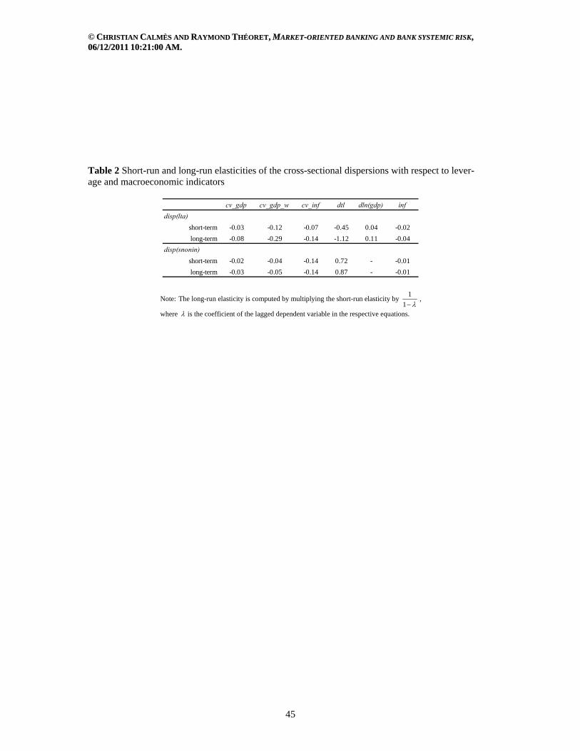
© CCHHRRIISSTTIIAANN CCAALLMMÈÈSS AANNDD RRAAYYMMOONNDD TTHHÉÉOORREETT,, MMAARRKKEETT--OORRIIEENNTTEEDD BBAANNKKIINNGG AANNDD BBAANNKK SSYYSSTTEEMMIICC RRIISSKK,, 0066//1122//22001111 1100::2211::0000 AAMM..
45
Table 2 Short-run and long-run elasticities of the cross-sectional dispersions with respect to lever-age and macroeconomic indicators
cv_gdp cv_gdp_w cv_inf dtl dln(gdp) inf
disp(lta)
short-term -0.03 -0.12 -0.07 -0.45 0.04 -0.02
long-term -0.08 -0.29 -0.14 -1.12 0.11 -0.04
disp(snonin)
short-term -0.02 -0.04 -0.14 0.72 - -0.01
long-term -0.03 -0.05 -0.14 0.87 - -0.01
Note: The long-run elasticity is computed by multiplying the short-run elasticity by 1
1 ,
where is the coefficient of the lagged dependent variable in the respective equations.
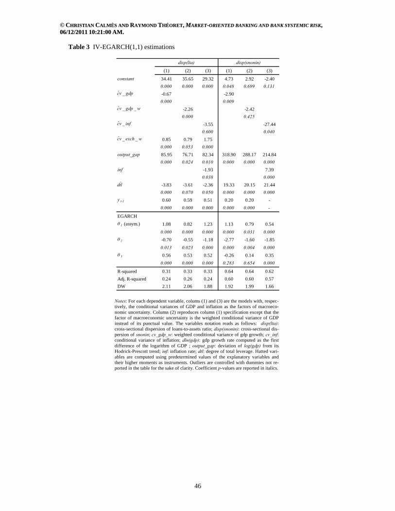
© CCHHRRIISSTTIIAANN CCAALLMMÈÈSS AANNDD RRAAYYMMOONNDD TTHHÉÉOORREETT,, MMAARRKKEETT--OORRIIEENNTTEEDD BBAANNKKIINNGG AANNDD BBAANNKK SSYYSSTTEEMMIICC RRIISSKK,, 0066//1122//22001111 1100::2211::0000 AAMM..
46
Table 3 IV-EGARCH(1,1) estimations
(1) (2) (3) (1) (2) (3)
constant 34.41 35.65 29.32 4.73 2.92 -2.40
0.000 0.000 0.000 0.048 0.699 0.131
-0.67 -2.90
0.000 0.009
-2.26 -2.42
0.000 0.425
-3.55 -27.44
0.600 0.040
dln(gdp) 0.85 0.79 1.75
0.000 0.053 0.000
output_gap 85.95 76.71 82.34 318.90 288.17 214.84
0.000 0.024 0.010 0.000 0.000 0.000
inf -1.93 7.39
0.038 0.000
-3.83 -3.61 -2.36 19.33 20.15 21.44
0.000 0.070 0.050 0.000 0.000 0.000
y t-1 0.60 0.59 0.51 0.20 0.20 -
0.000 0.000 0.000 0.000 0.000 -
EGARCH
θ 1 (assym.) 1.08 0.82 1.23 1.13 0.79 0.54
0.000 0.000 0.000 0.000 0.031 0.000
θ 2 -0.70 -0.55 -1.18 -2.77 -1.60 -1.85
0.013 0.023 0.000 0.000 0.004 0.000
θ 3 0.56 0.53 0.52 -0.26 0.14 0.35
0.000 0.000 0.000 0.283 0.654 0.000
R-squared 0.31 0.33 0.33 0.64 0.64 0.62
Adj. R-squared 0.24 0.26 0.24 0.60 0.60 0.57
DW 2.11 2.06 1.88 1.92 1.99 1.66
disp(snonin)disp(lta)
cv _ gdp
cv _ gdp _ w
ˆdtl
cv _ inf
cv _ exch _ w
Notes: For each dependent variable, colums (1) and (3) are the models with, respec-tively, the conditional variances of GDP and inflation as the factors of macroeco-nomic uncertainty. Column (2) reproduces column (1) specification except that the factor of macroeconomic uncertainty is the weighted conditional variance of GDP instead of its punctual value. The variables notation reads as follows: disp(lta): cross-sectional dispersion of loans-to-assets ratio; disp(snonin): cross-sectional dis-persion of snonin; cv_gdp_w: weighted conditional variance of gdp growth; cv_inf: conditional variance of inflation; dln(gdp): gdp growth rate computed as the first difference of the logarithm of GDP ; output_gap: deviation of log(gdp) from its Hodrick-Prescott trend; inf: inflation rate; dtl: degree of total leverage. Hatted vari-ables are computed using predetermined values of the explanatory variables and their higher moments as instruments. Outliers are controlled with dummies not re-ported in the table for the sake of clarity. Coefficient p-values are reported in italics.
© CCHHRRIISSTTIIAANN CCAALLMMÈÈSS AANNDD RRAAYYMMOONNDD TTHHÉÉOORREETT,, MMAARRKKEETT--OORRIIEENNTTEEDD BBAANNKKIINNGG AANNDD BBAANNKK SSYYSSTTEEMMIICC RRIISSKK,, 0066//1122//22001111 1100::2211::0000 AAMM..
47
Table A2 Conditional variances of GDP growth and inflation GDP growth inflation
Variable Coefficient p-value Variable Coefficient p-value
C 1.31 0.000 C 1.87 0.000
AR(1) 0.75 0.001 AR(1) 0.74 0.000
AR(2) -0.49 0.000
MA(1) -0.21 0.396 IGARCH equation
MA(2) 0.34 0.005
RESID-12
0.22 0.060
EGARCH equation GARCH-1 0.78 0.000
θ 1 (assymmetry coef.) -0.19 0.273
θ 2 0.59 0.000 R-squared 0.43
θ 3 -0.82 0.000 Adjusted R-squared 0.42
Durbin-Watson 1.76
R-squared 0.33
Adjusted R-squared 0.28
Durbin-Watson 1.57
Note: The EGARCH equation is estimated using specification (4), and the IGARCH, equation (16).

© CCHHRRIISSTTIIAANN CCAALLMMÈÈSS AANNDD RRAAYYMMOONNDD TTHHÉÉOORREETT,, MMAARRKKEETT--OORRIIEENNTTEEDD BBAANNKKIINNGG AANNDD BBAANNKK SSYYSSTTEEMMIICC RRIISSKK,, 0066//1122//22001111 1100::2211::0000 AAMM..
48
Table A3 Standard OLS estimations
(1) (2) (3) (1) (2) (3)
constant 33.59 33.86 31.76 14.80 14.00 3.57
0.000 0.000 0.000 0.274 0.288 0.746
cv_gdp 1.000 -2.971
0.378 0.056
cv_gdp_w -1.17 -3.22
0.634 0.584
cv_inf 7.84 -62.09
0.803 0.037
dln(gdp) 2.45 2.42 2.32
0.001 0.001 0.001
output_gap -3.69 -9.27 3.54 292.51 288.01 230.23
0.955 0.886 0.955 0.062 0.102 0.093
inf -1.39 -0.46
0.445 0.890
dtl -3.98 -3.78 -3.89 17.62 17.98 -1.41
0.223 0.257 0.244 0.002 0.002 0.844
y t-1 0.67 0.67 0.61 0.14 0.13 -
0.000 0.000 0.000 0.149 0.190 -
R-squared 0.40 0.39 0.38 0.66 0.65 0.66
Adj. R-squared 0.34 0.33 0.29 0.62 0.62 0.62
DW 2.22 2.24 2.20 1.95 1.97 1.79
disp(lta) disp(snonin)
Notes: For each dependent variable, Colums (1) and (3) are the models with, respec-tively, the conditional variances of GDP and inflation as the factors for macroeco-nomic uncertainty. Column (2) reproduces column (1) specification except that the factor of macroeconomic uncertainty is the weighted conditional variance of GDP in-stead of its ponctual value. The variables notation reads as follows: disp(lta): cross-sectional dispersion of loans-to-assets ratio; disp(snonin): cross-sectional dispersion of snonin; cv_gdp: conditional variance of gdp growth; cv_gdp_w: weighted conditional variance of gdp growth; cv_inf: conditional variance of inflation; dln(gdp): gdp growth rate computed as the first difference of the logarithm of GDP; output_gap: deviation of log(gdp) from its Hodrick-Prescott trend; inf: inflation rate; dtl: degree of total lever-age. Outliers are controlled with dummies not reported in the table for the sake of clar-ity. Coefficient p-values are reported in italics. The p-values are adjusted for het-eroskedacticity with the HAC matrix.

© CCHHRRIISSTTIIAANN CCAALLMMÈÈSS AANNDD RRAAYYMMOONNDD TTHHÉÉOORREETT,, MMAARRKKEETT--OORRIIEENNTTEEDD BBAANNKKIINNGG AANNDD BBAANNKK SSYYSSTTEEMMIICC RRIISSKK,, 0066//1122//22001111 1100::2211::0000 AAMM..
49
FIGURES
Figure 1 Canadian banks loans-to-assets ratio
47.5
50.0
52.5
55.0
57.5
60.0
62.5
65.0
97 98 99 00 01 02 03 04 05 06 07 08 09 10
%
Source: Canadian Bankers Association.
Figure 2 Canadian banks share of noninterest income in operating revenue
36
40
44
48
52
56
60
97 98 99 00 01 02 03 04 05 06 07 08 09 10
%
Source: Canadian Bankers Association.
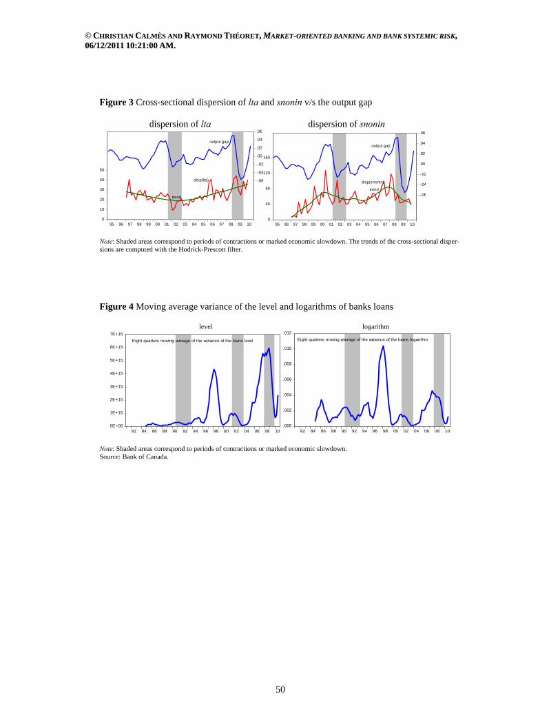
© CCHHRRIISSTTIIAANN CCAALLMMÈÈSS AANNDD RRAAYYMMOONNDD TTHHÉÉOORREETT,, MMAARRKKEETT--OORRIIEENNTTEEDD BBAANNKKIINNGG AANNDD BBAANNKK SSYYSSTTEEMMIICC RRIISSKK,, 0066//1122//22001111 1100::2211::0000 AAMM..
50
Figure 3 Cross-sectional dispersion of lta and snonin v/s the output gap dispersion of lta dispersion of snonin
0
10
20
30
40
50
-.06
-.04
-.02
.00
.02
.04
.06
95 96 97 98 99 00 01 02 03 04 05 06 07 08 09 10
output gap
disp(lta)
trend
0
40
80
120
160
-.06
-.04
-.02
.00
.02
.04
.06
95 96 97 98 99 00 01 02 03 04 05 06 07 08 09 10
output gap
disp(snonin)
trend
Note: Shaded areas correspond to periods of contractions or marked economic slowdown. The trends of the cross-sectional disper-sions are computed with the Hodrick-Prescott filter. Figure 4 Moving average variance of the level and logarithms of banks loans level logarithm
0E+00
1E+15
2E+15
3E+15
4E+15
5E+15
6E+15
7E+15
82 84 86 88 90 92 94 96 98 00 02 04 06 08 10
Eight quarters moving average of the variance of the loans level
.000
.002
.004
.006
.008
.010
.012
82 84 86 88 90 92 94 96 98 00 02 04 06 08 10
Eight quarters moving average of the variance of the loans logarithm
Note: Shaded areas correspond to periods of contractions or marked economic slowdown. Source: Bank of Canada.

© CCHHRRIISSTTIIAANN CCAALLMMÈÈSS AANNDD RRAAYYMMOONNDD TTHHÉÉOORREETT,, MMAARRKKEETT--OORRIIEENNTTEEDD BBAANNKKIINNGG AANNDD BBAANNKK SSYYSSTTEEMMIICC RRIISSKK,, 0066//1122//22001111 1100::2211::0000 AAMM..
51
Figure 5 Moving average variance of the level and logarithms of banks noninterest income level logarithm
0E+00
1E+12
2E+12
3E+12
4E+12
5E+12
82 84 86 88 90 92 94 96 98 00 02 04 06 08 10
Eight quarters moving average of the variance of the level of noninterest income
.00
.01
.02
.03
.04
.05
.06
.07
82 84 86 88 90 92 94 96 98 00 02 04 06 08 10
Eight quarters moving average of the varianceof the logarithm of noninterest income
Note: Shaded areas correspond to periods of contractions or marked economic slowdown. Source: Bank of Canada.
Figure 6 Scatter diagrams of the cross-sectional dispersions of lta and snonin with their respective cross-sectional covariance
lta snonin
-.0009
-.0008
-.0007
-.0006
-.0005
-.0004
-.0003
-.0002
-.0001
.0000
.02 .03 .04 .05 .06 .07
disp(lta)
cov(
lta)
correlation: -0.55
2010-Q1
2009-Q4
2010-Q2
2008-Q4
2009-Q1
1997-Q2
2006-Q1 2006-Q2
2008-Q3
2009-Q2
2009-Q3
2007-Q4
2008-Q22008-Q1
2007-Q3
-.007
-.006
-.005
-.004
-.003
-.002
-.001
.000
.001
.00 .04 .08 .12 .16 .20 .24
disp(snonin)
cov(
sno
nin
)
correlation: -0.91
2008-Q3
2008-Q4
2008-Q2
2008-Q1
2002-Q3