Credit Risk Spillovers, Systemic Importance and Vulnerability in Financial Networks

Inna Grinis SRC Discussion Paper No 27 January 2015

ISSN 2054-538X

Abstract How does the change in the creditworthiness of a financial institution or sovereign impact its creditors’ solvency? I address this question in the context of the recent European sovereign debt crisis. Considering the network of Eurozone member states, interlinked through investment cross-holdings, I model default as a multi-stage disease with each credit-rating corresponding to a new infection phase, then derive systemic importance and vulnerability indicators in the presence of financial contagion, triggered by the change in the creditworthiness of a network member. I further extend the model to analyse not only negative, but also positive credit risk spillovers. Keywords: financial networks, systemic risk, contagion, multi-stage disease. JEL classifications: F34, G01, G15 This paper is published as part of the Systemic Risk Centre’s Discussion Paper Series. The support of the Economic and Social Research Council (ESRC) in funding the SRC is gratefully acknowledged [grant number ES/K002309/1]. Inna Grinis, Department of Economics, London School of Economics and Political Science, Research Associate of the Systemic Risk Centre. Published by Systemic Risk Centre The London School of Economics and Political Science Houghton Street London WC2A 2AE All rights reserved. No part of this publication may be reproduced, stored in a retrieval system or transmitted in any form or by any means without the prior permission in writing of the publisher nor be issued to the public or circulated in any form other than that in which it is published. Requests for permission to reproduce any article or part of the Working Paper should be sent to the editor at the above address. © Inna Grinis submitted 2015

Credit Risk Spillovers, Systemic Importance and Vulnerability inFinancial Networks*

Inna Grinis1

Abstract

How does the change in the creditworthiness of a financial institution or sovereign im-pact its creditors′ solvency? I address this question in the context of the recent Europeansovereign debt crisis. Considering the network of Eurozone member states, interlinked throughinvestment cross-holdings, I model default as a multi-stage disease with each credit-ratingcorresponding to a new infection phase, then derive systemic importance and vulnerabilityindicators in the presence of financial contagion, triggered by the change in the creditworthi-ness of a network member. I further extend the model to analyse not only negative, but alsopositive credit risk spillovers.

JEL classification: F34, G01, G15.Keywords: financial networks, systemic risk, contagion, multi-stage disease.This version: November 2014Final version forthcoming in Complexity Economics

1 Introduction

Why does the downgrade of a European country not only raise the CDS spreads of that specificsovereign but also those of other Eurozone member states (Arezki et al. (2011))? More generally,how does the change in the creditworthiness of a financial institution or state impact its creditors′

solvency?This paper addresses such questions, investigating how a financial event that originates in one

specific country can spread beyond its borders, infecting other states like an epidemic. I modeldefault as a process - a multi-stage disease. Each credit-rating corresponds to an infection phase,during which default happens and therefore contagion is transmitted with a certain probability(Section 2). The model is general and could be applied not only to sovereigns, but to any financialinstitutions such as banks, firms, etc. interlinked by mutual financial liabilities. However, givendata availability and recent events, I illustrate its workings in the context of the European sovereigndebt crisis. The seventeen member states are the nodes in the network, and the weighted directededges between them measure cross-country investment flows (Fig.1).

My goal is to develop indicators of node importance and vulnerability by investigating howthe exogenous change in the creditworthiness of one of the financial network members impacts thecreditworthiness of all the other ones (Section 3). Firstly, I derive some analytical indices fromthe early time properties of the model, then I employ computer simulations to measure systemic

1Department of Economics and SRC, London School of Economics and Political Science, Houghton Street,London, WC2A 2AE, UK. Email: I.Grinis@lse.ac.uk.

*I am grateful to the Financial Markets Group at the LSE and the Deutsche Bank for awarding me the runner-upDeutsche Bank Prize in Financial Risk Management and Regulation for an earlier version of this paper. I would alsolike to thank two anonymous referees for their valuable comments and suggestions, and Dr. Chryssi Giannitsaroufor supervising my undergraduate thesis at the University of Cambridge, during which many of the ideas furtherdeveloped here originated, and that won the 2013 Adam Smith Best Dissertation Prize. This work was supportedby the Economic and Social Research Council [grant number 200900383].

1

importance and vulnerability. Both indicators are systemic in the sense that they not only capturethe immediate effect of the “exogenous risk that hits the system” (such as an aggregate exogenousshock or an idiosyncratic shock to one of the nodes in the network), but also the “endogenous riskgenerated by the system itself” (Zigrand (2014)). The system here is the network and the aim isto find indicators that will take into account how the structure of the links shapes and propagatesan initial exogenous shock. I also extend the model to analyse how the same feedback mechanismsthat generate endogenous risk, could set off a process of positive contagion, reversing negativemarket sentiments (Section 4).

This paper can be related to the existing vast literature on financial contagion. At the twoextremes, contagion is classified as pure - when a herd of investors drives apparently healthy andunrelated economies towards sunspot equilibria - or fundamentals-based (Masson (1999)). In realityhowever, spillovers are complex and encompass both features: they spread through real or financialchannels, while still retaining some randomness driven by market sentiments. I try to capture thisduality by on the one hand considering a financial network of cross-country investment flows, whileon the other hand making downgrades happen stochastically. Indeed, the probability that an agenttransmits the “default disease” to its network neighbours depends on both: its actual credit rating(an agent with a lower credit-rating, i.e. in a more advanced infection phase, transmits the negativecontagion at a higher rate) and the interaction intensities (a stronger mutual relation increases thetransmission probability).2

One of the first models studying financial contagion on networks is Allen & Gale (2000). Theauthors extend Diamond & Dybvig (1983) to a four banks system, showing how the completenessand distribution of interconnections determine the extent of spillovers following a bank-specificshock. With evenly allocated deposits, contagion may be completely avoided, whereas in anincomplete system, a cascade of failures might emerge. Allen & Babus (2009) give an overview ofsome recent developments in this field. Espinosa-Vega & Sole (2011) build an interbank exposuremodel, simulating credit and liquidity shocks. Their algorithm starts with the default of a country′sbanking system shifting the balance sheets of yet solvent banks and triggering new failures. Ina similar spirit, Elliott et al. (2014) construct a theoretical model in which the market valuesof organisations are interdependent through the network of cross-holdings. The default of anorganisation (bank or country) changes the values of all the other ones inducing those, whose newvalues fall below certain specified “bankruptcy thresholds”, to fail as well. The contagion processcontinues until either the algorithm converges with no new failures, or no solvent organisationremains.

One of the main criticisms of such studies has been their limited scope given the “extremelyrare” nature of “contagious failures” (Upper (2006)). Here, instead of analysing how financialcontagion results from the initial default of a bank or country, I model the default process itself,and investigate how financial contagion can be triggered by simple changes in the creditworthinessof one of the network members.

The credit-rating determination of a bank (Bissoondoyal-Bheenick & Treepongkaruna (2009))or a sovereign (Melliosa & Paget-Blanc (2006), Afonso (2003), Cheung (1996)) have been tradi-tionally studied using econometric ordered-response models with creditworthiness as the latentvariable. The problem with this approach is that it completely ignores the possibility of credit riskspillovers between financial entities. Unfortunately, once we model agents′ interactions explicitly

2For a discussion of the relative importance of trade linkages versus macroeconomic similarities in currency crises,see Eichengreen et al. (1996). Gerlach & Smets (1995), Corsetti et al. (1999), and Pesenti & Tille (2000) presenttheoretical models of contagious transmission with applications to the Asian currency crisis and the ERM turmoil.

2

through a network, and admit that their creditworthiness levels are interrelated and determinedsimultaneously, this econometric framework can no longer be used because of endogeneity.

I propose a different approach to studying creditworthiness and credit risk spillovers that takesinspiration from the epidemiology literature. Indeed, the highly interconnected and complex na-ture of the global financial system has spurred researchers to draw interesting and original par-allels between financial networks, ecosystems (May et al. (2008)), epidemiology, and even engi-neering (Haldane (2009)). Demiris et al. (2014) explore financial contagion in the context of aSusceptible-Infected-Recovered (SIR) model, emphasising its advantages over more conventionalmodelling approaches. In particular, the SIR framework allows them to model explicitly thecountry-interdependencies that are essential to the propagation of a crisis, measure crisis sever-ity by a threshold parameter instead of composite macroeconomic indicators as in Kaminsky &Reinhart (1998), and evaluate potential policy interventions.

Beside these theoretical advances, an increased interest in complexity economics and agent-based modelling have recently re-emphasized the usefulness of computer simulations in under-standing complex systems (Farmer & Foley (2009)). For instance, Caporale et al. (2008) developa multinomial model using time series data on stock returns during the East Asian crisis (1997),and thereby disentangle potentially destabilizing connections that could signal the inception of acontagion process. Gai et al. (2011) experiment with different parameter configurations, studyinghow complexity and concentration affect the resilience of a financial system. I follow this trend anduse computer simulations not only to derive indicators of systemic importance and vulnerability,but also to incorporate positive contagion, thereby making the model more complex, interesting,and realistic.

2 Credit Risk Spillovers

2.1 The determinants of creditworthiness

Consider a network with n ∈ N nodes. As an illustration, Figure 1 depicts the network of theseventeen Eurozone member states. Since the ultimate goal is to study credit risk spillovers,the links between nodes should reflect the intensity of potential contagion flows. Fig.1 looks atthe 2011 cross-border Total Portfolio Investment (TPI) flows. The data is available from theIMF (Consolidated Portfolio Investment Survey). TPI flows are reported on an annual basis andinclude long & short term equities and debt-securities. I transform the data into investmentshares since absolute values of investment flows vary with the overall size of the economy andneed to be normalised. Formally, I define the weighted, directed link from j to i (vij) as theproportion of country i’s total investment flowing into j. Intuitively, the arcs follow contagionflows so that the larger vij, the more significant the direct potential spillover from j’s downgradeonto i’s creditworthiness. In Fig.1, nodes are coloured and weighted by their average degrees12

{∑i vij +

∑j vij

}.

Investment shares vij can be summarized in an n×n adjacency matrix V (Table 1). Note thatvii = 0 (foreign investment only) and row i gives the distribution of country i’s TPI across otherEurozone member states. For instance, Austria invests 21.46% into Germany and only 0.64% intoGreece. Rows do not sum up to 100% because countries also invest in non-EZ states. In general,vij 6= vji, e.g. Italy invests 26.22% into Luxembourg, while Luxembourg only invests 4.64% intoItaly.

3

Figure 1: Eurozone network, 2011 Total Portfolio Investment (TPI) shares

Table 1: Adjacency matrix, 2011 Total Portfolio Investment (TPI) shares (percentages)

AUS BE CY EST FIN FR DE GRE IRE IT LUX MAL NTH PT SK SL SPAUS 0 1.319 0.140 0.023 1.368 8.524 21.456 0.638 3.705 7.398 8.434 0.010 7.327 0.525 0.790 0.710 3.538BE 2.265 0 0.032 0.002 0.838 18.459 6.689 0.455 5.700 4.845 19.111 0.006 14.661 0.730 0.195 0.226 5.172CY 0.496 1.838 0 0 0.411 4.291 2.372 27.833 3.708 3.448 2.419 0 2.121 0.300 0.003 0.112 0.924EST 3.113 3.352 0.311 0 7.328 14.679 7.328 0.096 6.346 7.807 11.997 0.024 8.357 0.431 0.455 0.216 1.461FIN 1.425 0.668 0.036 0.094 0 8.007 10.144 0.291 5.159 2.243 8.755 0 5.742 0.398 0.022 0.079 2.156FR 3.072 4.340 0.012 0.001 0.678 0 11.303 0.587 4.138 10.761 6.104 0.038 11.883 1.381 0.039 0.104 8.281DE 3.865 1.415 0.042 0.002 1.053 12.668 0 0.516 5.263 7.299 16.218 0.004 9.968 0.935 0.180 0.127 6.878

GRE 0.929 0.330 3.393 0 0.052 3.284 2.727 0 2.394 1.857 7.902 0 2.242 0.296 0 0 0.641IRE 0.358 0.544 0.009 0.008 0.594 5.374 7.174 0.144 0 5.724 2.248 0.011 3.820 2.633 0.017 0.009 2.031IT 1.719 0.810 0.007 0 0.328 13.094 10.381 0.430 8.634 0 26.215 0.022 6.483 0.690 0.035 0.116 4.505

LUX 1.036 1.792 0.045 0.009 0.648 9.750 12.381 0.103 2.711 4.635 0 0.019 5.164 0.264 0.019 0.023 2.299MAL 1.939 1.011 0.107 0 0.308 3.942 5.765 0.950 5.191 2.309 2.720 0 4.851 1.134 0.175 0.942 2.677NTH 2.255 1.673 0.015 0.002 1.181 11.271 15.964 0.228 3.445 3.487 5.355 0.004 0 0.807 0.037 0.024 3.920PT 1.372 1.762 0 0 0.416 9.599 5.298 1.327 20.645 9.603 6.566 0 7.113 0 0.050 0.028 11.795SK 5.286 1.173 0.527 0 2.431 9.394 4.222 1.154 8.663 7.995 2.864 0 6.088 4.343 0 2.444 15.855SL 6.269 3.923 0.040 0.015 0.805 13.337 18.605 2.721 2.348 8.654 4.082 0 7.023 0.953 1.227 0 2.259SP 1.678 2.054 0 0 0.358 13.227 8.685 0.872 6.806 15.753 9.975 0 9.567 3.933 0 0 0

Source: Coordinated Portfolio Investment Survey (CPIS), IMFcf. Table 8: Geographic Breakdown of Total Portfolio Investment Assets: Total Portfolio Investment, http://cpis.imf.org/

The adjacency matrix is obtained by dividing the original entries in the CPIS matrix by the total value of investment for each country.

4

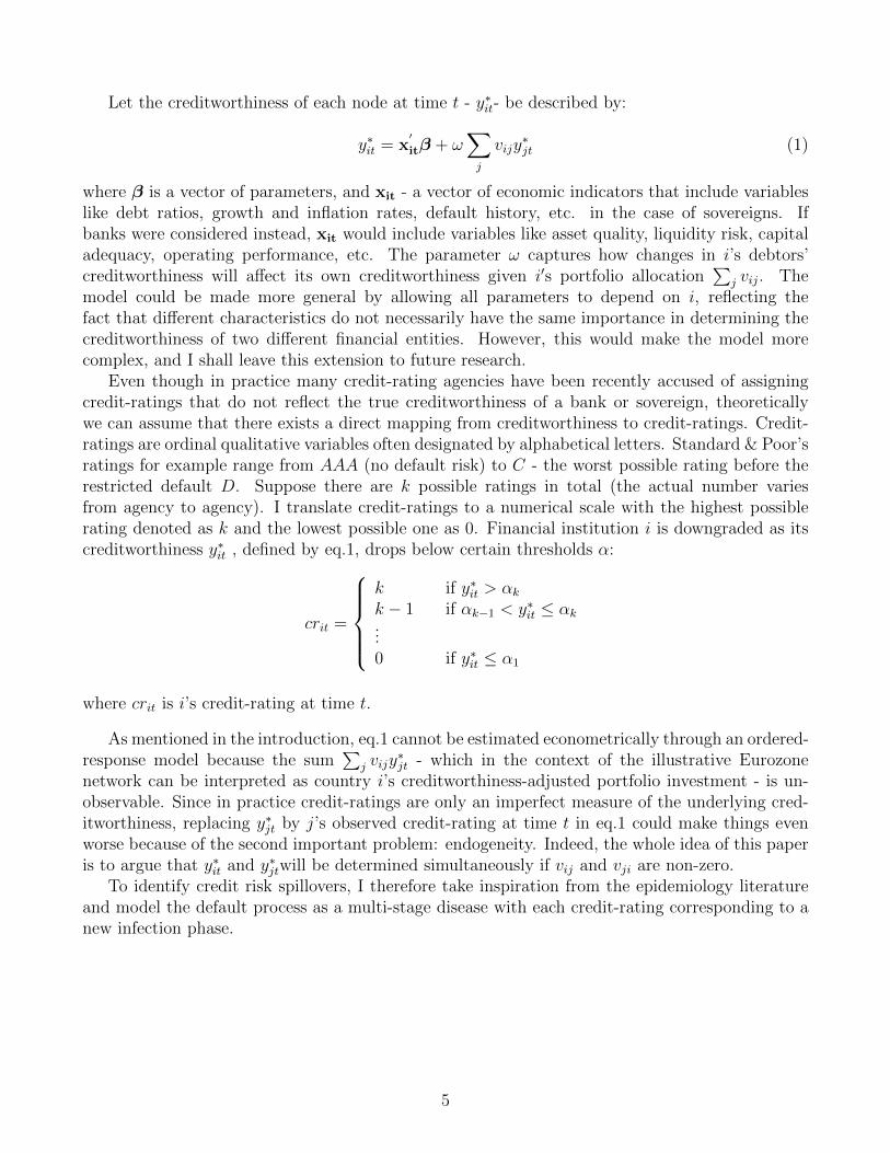
Let the creditworthiness of each node at time t - y∗it- be described by:

y∗it = x′

itβ + ω∑j

vijy∗jt (1)

where β is a vector of parameters, and xit - a vector of economic indicators that include variableslike debt ratios, growth and inflation rates, default history, etc. in the case of sovereigns. Ifbanks were considered instead, xit would include variables like asset quality, liquidity risk, capitaladequacy, operating performance, etc. The parameter ω captures how changes in i’s debtors’creditworthiness will affect its own creditworthiness given i′s portfolio allocation

∑j vij. The

model could be made more general by allowing all parameters to depend on i, reflecting thefact that different characteristics do not necessarily have the same importance in determining thecreditworthiness of two different financial entities. However, this would make the model morecomplex, and I shall leave this extension to future research.

Even though in practice many credit-rating agencies have been recently accused of assigningcredit-ratings that do not reflect the true creditworthiness of a bank or sovereign, theoreticallywe can assume that there exists a direct mapping from creditworthiness to credit-ratings. Credit-ratings are ordinal qualitative variables often designated by alphabetical letters. Standard & Poor’sratings for example range from AAA (no default risk) to C - the worst possible rating before therestricted default D. Suppose there are k possible ratings in total (the actual number variesfrom agency to agency). I translate credit-ratings to a numerical scale with the highest possiblerating denoted as k and the lowest possible one as 0. Financial institution i is downgraded as itscreditworthiness y∗it , defined by eq.1, drops below certain thresholds α:

crit =

k if y∗it > αk

k − 1 if αk−1 < y∗it ≤ αk...0 if y∗it ≤ α1

where crit is i’s credit-rating at time t.

As mentioned in the introduction, eq.1 cannot be estimated econometrically through an ordered-response model because the sum

∑j vijy

∗jt - which in the context of the illustrative Eurozone

network can be interpreted as country i’s creditworthiness-adjusted portfolio investment - is un-observable. Since in practice credit-ratings are only an imperfect measure of the underlying cred-itworthiness, replacing y∗jt by j’s observed credit-rating at time t in eq.1 could make things evenworse because of the second important problem: endogeneity. Indeed, the whole idea of this paperis to argue that y∗it and y∗jtwill be determined simultaneously if vij and vji are non-zero.

To identify credit risk spillovers, I therefore take inspiration from the epidemiology literatureand model the default process as a multi-stage disease with each credit-rating corresponding to anew infection phase.

5

2.2 The Default Process

2.2.1 From the “Susceptible - Infected” (SI) model to the “Solvent-Default”(SD)one

The SI model was initially developed to analyse human disease spreading on contact networks (Ker-mack & McKendrick (1932)). Although the process of infection is much more complex than thistwo-states model, it remains a “useful simplification” to the extent that it captures the contagiondynamics “happening at the level of networks” (Newman (2012)).

At any point in time, an individual is either susceptible or infected. Suppose that you aresusceptible - which happens with probability si. To catch the disease, one of your neighbours mustalready be infected - the probability of this event is dj. Since this infected neighbour transmitsthe disease at rate δ, the probability that you become infected at any point in time is:

ddidt

= δ∑j

vij {sidj} (2)

where the accolades on the right-hand side take into account the correlations (joint probabilities)for nodes i and j to have the specified states, e.g. {sidj} is the “average probability that i issusceptible and j is infected at the same time” (Newman (2012)). Interaction intensities vij playa crucial role in eq.2. Two individuals, interacting with exactly the same people, could havecompletely different infection probabilities if the first person’s contacts mainly include alreadycontaminated individuals, whereas the second one is more interlinked with still healthy people.

Translating the SI framework into a “Solvent-Default” (SD) one is rather trivial. We can simplythink of the interaction intensity vij as the strength of the potential contagion flow from j to i. Forinstance, in the Eurozone network illustrated in Fig.1, the vij’s will be the TPI shares. Eq.2 impliesthat two countries, Z and W, investing in exactly the same sovereigns with the only difference that∑

j vZj puts relatively higher weights on countries with larger dj than∑

j vWj, would have verydifferent default probabilities. In particular, Z’s default probability would be larger than W’s.Notice that this discrepancy would occur not because of a difference in dj, but as a consequenceof different TPI shares’ distributions.

Unfortunately, this simple SD framework is inappropriate for the investigation of credit riskspillovers, because it only models two states: Solvent and Default. In reality, a solvent financialinstitution does not suddenly declare bankruptcy; it undergoes a process of rating downgrades,which I model as a multi-stage disease.

2.2.2 Default as a multi-stage disease

Modeling default as a multi-stage disease makes the previous framework more complex, but allowsfinancial institutions to differ in how solvent they are.

It might be insightful to think about each credit-rating downgrade as marking the beginningof a new infection phase. Let θ(crit) ∈ [0; 1] be the rate at which institution i with credit-ratingcrit transmits the “default disease” to its creditors. An institution with lower creditworthiness, i.e.in a more advanced infection phase, is more likely to default itself. It should therefore be morevirulent and transmit the default contagion at a higher rate, i.e. θ(crit) must be decreasing in crit.

For simplicity, suppose there are only four possible credit-ratings (k = 4): A, B, C, and D. Letait, bit, cit and dit denote the probabilities that institution i has rating A, B, C, or D respectively

6

at time t. Clearly:ait + bit + cit + dit = 1

because an institution must be rated at any point in time.Further, let the transmission rates be: θ(A) = 0 and θ(cr) ∈ (0; 1] for any cr 6= A.Given the network of n financial institutions or states, i can be downgraded from A to B

for two reasons. Firstly, as a result of a credit risk spillover from one of its debtors. For this, imust start with rating A which happens with probability ait. Moreover, one of its debtors musthave rating crjt ∈{B, C, D} - which happens with probabilities zjt = {bjt, cjt, djt} respectively- and transmit the contagion at rate θ(crjt). Secondly, i could also be downgraded because ofan exogenous deterioration in one of its characteristics xit. The following differential equationdescribes the probability that i loses credit-rating A:

daidt

= −ω∑j

vij {aitzjt} θ(crjt) + βAdxidt

(3)

Similarly, the probability that i has rating B increases in i’s probability of being downgradedfrom A to B, but decreases in i’s probability of being downgraded from B to C:

dbidt

= ω∑j

vij {aitzjt} θ(crjt)− ω∑j

vij {bitzjt} θ(crjt) + βB dxidt

(4)

The differential equation for rating C is described in a similar way:

dcidt

= ω∑j

vij {bitzjt} θ(crjt)− ω∑j

vij {citzjt} θ(crjt) + βC dxidt

(5)

Finally, the last downgrade from C to D corresponds to the default after which the countryexits the system:

ddidt

= ω∑j

vij {citzjt} θ(crjt) + βD dxidt

(6)

where the parameter on the exogenous shock β is allowed to depend on the credit rating underconsideration.

There is one important difference between this extended SD model and the existing multi-stage disease ones from the epidemiology literature. In the latter, “the only stochastic step [...] istransmission of the disease”(Jaquet & Pechal (2009)) - i.e. once an individual becomes infected, shewill traverse all the disease stages deterministically until reaching the final phase (e.g. becomingresistant) - whereas in the multi-stage SD model, progression towards the next infection phase stilldepends on contact with already contaminated units. 34

3Note that the infection phases of the node’s debtors do not have to be “more advanced” than its own contam-ination phase in order to make him progress to the next infection stage. Consider the following example: countryX currently has rating B and has only two debtors: countries Y and Z, both with ratings A, i.e. in “less advanced”infection phases than itself. If country Y is downgraded from A to B, this will increase the probability of countryX being downgraded to C, i.e. there will still be a credit-risk spillover despite the fact that country Y was initiallyless infected than country X.

4Aside from the economic content of this paper, there is a need to properly understand the dynamics andphase diagrams of a multi-stage epidemic model in which progression to the next infection phase depends oninteraction with other contaminated people. Although such a model could not be applied in common epidemic

7

Figure 2: Given the initial vector of ratings (2012 Q4), this experiment simulates the contagion process showingthe evolutions of the ratings for each country.

2.3 Computer Simulations

The model presented in the previous section has no closed form solution. To analyse it, I havewritten a graph-based computer algorithm whose main component is a function called spillovers.This function takes as arguments an adjacency matrix V, a transmission-rates vector θ, and thevector of initial ratings rat0. Firstly, it associates to each country i a transmission rate θ(cri) thatdepends on its rating. After computing country-specific downgrade probabilities using eq.7, somecountries are stochastically downgraded:

Pr(i downgraded) = ω∑j

vijθ(crj) (7)

Here, ω ∈ R+ captures the overall spillovers’ magnitude (the “severity” of the disease) and allowsto change the speed of the simulations without altering downgrade rankings.

Spillovers’ output is a new vector of ratings: rat1. The contagion function recalls spilloversuntil all countries default - which happens at time Td - using the spillovers’ previous ratingsoutput vector as the new input at each iteration step, and producing a matrix with columns:rat0, rat1, rat2, ..., ratTd

. Technically, one country usually remains solvent. Since the simulationstops when all but one country default, this solvent country also defaults at Td.

Fig.2 illustrates the computer simulation on the Eurozone TPI network with the fourth quarter2012 S&P’s credit ratings as rat0. I only use the first seventeen S&P’s ratings, grouping together

settings such as the transmission of a viral infection, it could be very useful in understanding contagious mentalillnesses. For instance, Joiner & Katz (1999) investigate 40 studies conducted between 1976-1997 “that examinedthe relationship between two non-genetically related individuals’ levels of depression or negative mood”, and findevidence of significant contagion for all the 12 studies that analysed syndromal depression spillovers between “collegeroommates, dating couples, young spouses, elderly spouses, and relatives.” Interestingly, they also find that only13 of the 28 studies dealing with negative mood, report significant spillovers, concluding that “depressive symptomsare [. . . ] more contagious than negative mood.” This agrees with the framework used in this paper, wherebymore advanced infection phases are presented as more virulent. Hence, the model analysed in section 2 could helpunderstand the transition from a moderate state of depression or even a simple negative mood to more severephases.

8

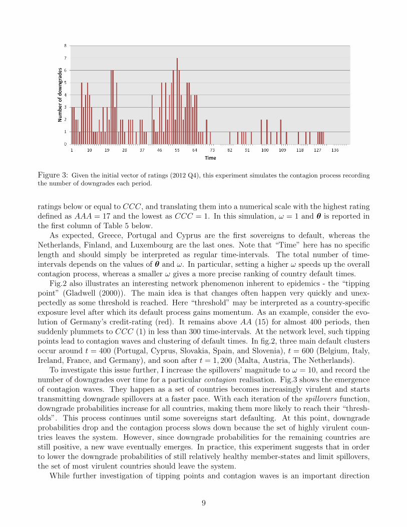
Figure 3: Given the initial vector of ratings (2012 Q4), this experiment simulates the contagion process recordingthe number of downgrades each period.

ratings below or equal to CCC, and translating them into a numerical scale with the highest ratingdefined as AAA = 17 and the lowest as CCC = 1. In this simulation, ω = 1 and θ is reported inthe first column of Table 5 below.

As expected, Greece, Portugal and Cyprus are the first sovereigns to default, whereas theNetherlands, Finland, and Luxembourg are the last ones. Note that “Time” here has no specificlength and should simply be interpreted as regular time-intervals. The total number of time-intervals depends on the values of θ and ω. In particular, setting a higher ω speeds up the overallcontagion process, whereas a smaller ω gives a more precise ranking of country default times.

Fig.2 also illustrates an interesting network phenomenon inherent to epidemics - the “tippingpoint” (Gladwell (2000)). The main idea is that changes often happen very quickly and unex-pectedly as some threshold is reached. Here “threshold” may be interpreted as a country-specificexposure level after which its default process gains momentum. As an example, consider the evo-lution of Germany’s credit-rating (red). It remains above AA (15) for almost 400 periods, thensuddenly plummets to CCC (1) in less than 300 time-intervals. At the network level, such tippingpoints lead to contagion waves and clustering of default times. In fig.2, three main default clustersoccur around t = 400 (Portugal, Cyprus, Slovakia, Spain, and Slovenia), t = 600 (Belgium, Italy,Ireland, France, and Germany), and soon after t = 1, 200 (Malta, Austria, The Netherlands).

To investigate this issue further, I increase the spillovers’ magnitude to ω = 10, and record thenumber of downgrades over time for a particular contagion realisation. Fig.3 shows the emergenceof contagion waves. They happen as a set of countries becomes increasingly virulent and startstransmitting downgrade spillovers at a faster pace. With each iteration of the spillovers function,downgrade probabilities increase for all countries, making them more likely to reach their “thresh-olds”. This process continues until some sovereigns start defaulting. At this point, downgradeprobabilities drop and the contagion process slows down because the set of highly virulent coun-tries leaves the system. However, since downgrade probabilities for the remaining countries arestill positive, a new wave eventually emerges. In practice, this experiment suggests that in orderto lower the downgrade probabilities of still relatively healthy member-states and limit spillovers,the set of most virulent countries should leave the system.

While further investigation of tipping points and contagion waves is an important direction

9

for future research, the next step and main goal of this paper is to use the model and the com-puter algorithm presented in this section to derive indicators of node/country importance andvulnerability.

3 Systemic Importance and Vulnerability

3.1 Early-time properties: some analytical results

Consider again the model from subsection 2.2.2 and suppose that all n financial institutions startwith the best possible credit-rating A, i.e. ai0 = 1 for any i. Now, let one of the institutions beexogenously downgraded. Afterwards, in order to disentangle credit risk spillovers from exogenouseconomic fundamentals’ deterioration, set dxi

dt= 0 for any i and t.

Which institutions are most likely to be downgraded from A in this early period? To answerthis question, note that since cit = 0, dit = 0, and ait + bit = 1 for any i, one only needs to focuson eq.4 which can be rewritten as:

dbidt

= ω∑j

vijbjtθ(B)

because ait → 1 and θ(A) = 0. In matrix notation:

db

dt= ωθ(B)Vb

which is a system of differential equations that has a solution of the following form:

b(t) =n∑

r=1

ur(0) exp(ωθ(B)κrt)µr

where κr’s and µr’s are respectively the eigenvalues and eigenvectors of the matrix V and ur(0)’sare some constants. Let κ1 and µ1 denote the largest eigenvalue and its associated eigenvectorrespectively:

b(t) ∼ exp(ωθ(B)κ1t)µ1 (8)

Hence, thinking of b(t) as an indicator of early-time vulnerability, eq.8 shows that it will bedirectly proportional to V′s right leading eigenvector κ1. In the network literature, this metric iscalled (right) eigenvector centrality (Newman (2012)).

A closely-related indicator can be constructed to gauge early-time importance. The trick hereconsists in taking the transpose of the adjacency matrix: W = VT so that wij = vTij = vji. Nowrow i of W gives the distribution of all network members’ investment shares into i. Let σ(t) denotethe vector of early-time importance. I want an indicator that ranks higher those countries, whosemajor creditors are themselves more important. The differential equation of the form:

dσidt

= η∑j

vjiσjt

shows that the importance of node i is indeed increasing in the importance of its creditors σjt andthe proportion that they invest into i : vji. Rewriting in matrix notation and performing the sameexercise as above one gets:

10

σ(t) ∼ exp(ηλ1t)π1

where λ1 and π1 are the leading left eigenvalue and eigenvector of the matrix V. Hence the vectorof early-time importance will be proportional to the left eigenvector centrality.

3.2 Late-time properties: systemic indicators

One of the main goals of this paper is to measure systemic importance and vulnerability. To buildindicators that take into account every possible feedback mechanism generated by the networkstructure, I need to switch from the early-time when the contagion process just sets off, to thetime when the countries have traversed their default processes almost completely.

Conceptually, the experiment remains the same: all n institutions start with the best possiblecredit-rating A, and one of the institutions is exogenously downgraded. Nevertheless, the keydifference is that instead of asking which institutions are most likely to be downgraded to rating Bfirst, I now ask how long will it take for institution i to default? How does this time compare to thetime needed for other institutions to default? What if I pick and downgrade another institutionfirst?

A bit of imagination leads to define the following two possible indicators of systemic importance:

• All-default time: T id gives the time when all of the nodes in the network default after the

initial exogenous downgrade of node i.

• First-default time: F id gives the time of the first default in the network after the initial

exogenous downgrade of node i.

Intuitively, the initial downgrade of a systemically more important country should lead to quickerFirst- and All- default times (smaller F i

d and T id).

In the same spirit, the default time of node i after the initial downgrade of node j - V ji -

identifies i’s systemic vulnerability to j. If i is more vulnerable to l than to h, we should observe:V li < V h

i . A summary indicator is i’s average systemic vulnerability :

V uli =1

n

∑j

V ji

3.3 Application to the Eurozone Sovereign debt crisis

To see how these different analytical and simulation-based indicators relate to each other, tables 2and 3 report the computed rankings and indicators for all 17 member-states using the TPI sharesas the adjacency matrix (Table 1). Countries are arranged according to All-default (Td) andVulnerability (V ul) rankings respectively.

Germany alternates with France in the role of the most systemically important Eurozone coun-try depending on the indicator used. Although Luxembourg is a small country, it is consistentlyranked second/third because other EZ members invest substantial shares into it: between 2.4%(Cyprus) and 26.2% (Italy). Remarkably, many countries (e.g. the Netherlands, Italy, Ireland,Spain) keep exactly the same positions in all importance rankings. In terms of vulnerability, thepicture is less clear-cut. Slovenia and Slovakia are ranked highest by different indicators. Greece

11

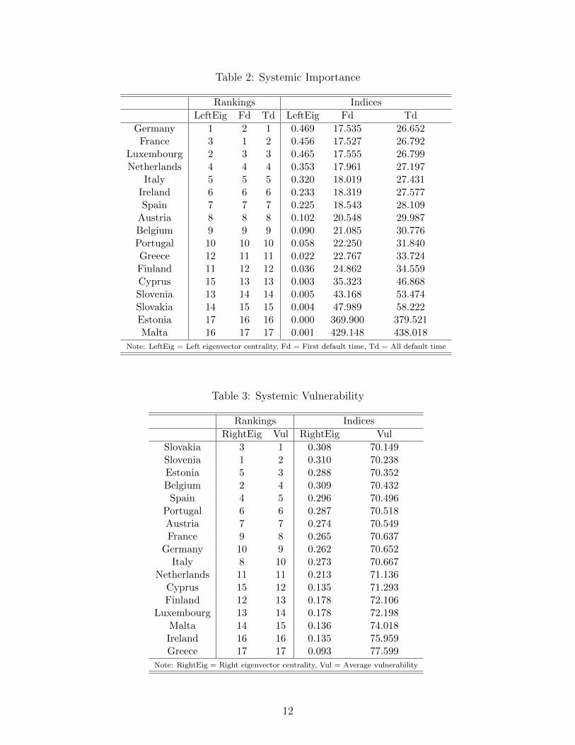
Table 2: Systemic Importance

Rankings Indices

LeftEig Fd Td LeftEig Fd Td

Germany 1 2 1 0.469 17.535 26.652France 3 1 2 0.456 17.527 26.792

Luxembourg 2 3 3 0.465 17.555 26.799Netherlands 4 4 4 0.353 17.961 27.197

Italy 5 5 5 0.320 18.019 27.431Ireland 6 6 6 0.233 18.319 27.577Spain 7 7 7 0.225 18.543 28.109

Austria 8 8 8 0.102 20.548 29.987Belgium 9 9 9 0.090 21.085 30.776Portugal 10 10 10 0.058 22.250 31.840Greece 12 11 11 0.022 22.767 33.724Finland 11 12 12 0.036 24.862 34.559Cyprus 15 13 13 0.003 35.323 46.868Slovenia 13 14 14 0.005 43.168 53.474Slovakia 14 15 15 0.004 47.989 58.222Estonia 17 16 16 0.000 369.900 379.521Malta 16 17 17 0.001 429.148 438.018

Note: LeftEig = Left eigenvector centrality, Fd = First default time, Td = All default time

Table 3: Systemic Vulnerability

Rankings Indices

RightEig Vul RightEig Vul

Slovakia 3 1 0.308 70.149Slovenia 1 2 0.310 70.238Estonia 5 3 0.288 70.352Belgium 2 4 0.309 70.432

Spain 4 5 0.296 70.496Portugal 6 6 0.287 70.518Austria 7 7 0.274 70.549France 9 8 0.265 70.637

Germany 10 9 0.262 70.652Italy 8 10 0.273 70.667

Netherlands 11 11 0.213 71.136Cyprus 15 12 0.135 71.293Finland 12 13 0.178 72.106

Luxembourg 13 14 0.178 72.198Malta 14 15 0.136 74.018Ireland 16 16 0.135 75.959Greece 17 17 0.093 77.599

Note: RightEig = Right eigenvector centrality, Vul = Average vulnerability

12

Table 4: Robustness simulations

Simulation 2 (different θ) Simulation 3 (different ω)

Fd2 Td2 Vul2 Fd3 Td3 Vul3Index R Index R Index R Index R Index R Index R

Austria 74.290 8 86.760 8 617.601 7 27.339 8 56.691 8 128.670 8Belgium 81.050 9 94.200 9 617.332 3 28.277 9 57.834 9 127.504 1Cyprus 232.962 13 253.988 13 618.879 12 62.441 13 90.615 13 132.343 11Estonia 4231.200 16 4243.600 16 617.475 5 714.407 16 744.862 16 127.866 4Finland 126.770 12 139.011 12 620.943 14 36.237 11 65.681 12 134.305 13France 39.512 2 50.385 2 617.674 8 20.961 1 50.164 1 129.066 10

Germany 39.140 1 49.989 1 617.777 9 21.018 3 50.758 2 128.825 9Greece 83.683 10 104.333 10 624.523 17 37.772 12 64.946 11 150.784 16Ireland 49.159 6 62.703 6 622.238 16 22.818 6 52.158 6 151.436 17Italy 44.847 5 57.869 5 617.872 10 22.062 5 51.954 4 128.310 7

Luxembourg 39.627 3 50.399 3 619.867 13 20.974 2 51.633 3 138.959 14Malta 4525.400 17 4537.400 17 621.473 15 879.368 17 909.022 17 139.594 15

Netherlands 43.846 4 56.643 4 618.813 11 21.790 4 52.097 5 132.440 12Portugal 93.860 11 107.579 11 617.499 6 30.652 10 59.459 10 127.976 5Slovakia 364.315 15 377.453 15 616.502 1 83.556 15 115.409 15 127.579 2Slovenia 301.904 14 315.323 14 616.656 2 74.789 14 106.016 14 127.666 3

Spain 51.559 7 64.515 7 617.398 4 23.247 7 52.769 7 127.978 6

Note: R = Ranking

is ranked lowest probably because most of its investment flows into the UK with only 26.1% re-maining in the EZ. The interpretation of all the results is necessarily limited and future researchshould test the model on a larger dataset.

To check whether these results depend on the specific values assumed for θ and ω in thecomputer simulations, table 4 contains the results from two additional simulations: with a differentθ (simulation 2), and a different ω (simulation 3). I arrange countries alphabetically and report allthree simulation-based indicators. The parametrization of all simulations is summarized in table 5.

Rankings remain almost identical. Indeed as table 6 shows, the ranking correlations of All-default times, First-default times, and Vulnerability indicators across all three simulations arealmost perfect.

Table 6 also sheds more light on the relationships between different indicators. There is signifi-cant positive correlation within the two sets of importance and vulnerability rankings, but negativecorrelation between them (bottom-left part). The positive within correlation suggests that the in-dicators capture indeed the same node characteristic (either importance or vulnerability). Thedifference in rankings reflects the presence of endogenous risk generated by the network structureitself. The negative between correlation shows that the sets of most important and most vulnerablecountries do not overlap. Such a situation may lead to moral hazard problems if the most system-ically important players do not bear the full network costs of idiosyncratic shocks affecting them,i.e. they do not internalize the negative externality generated on the most vulnerable countries,and take on more risks than would be socially desirable.

13

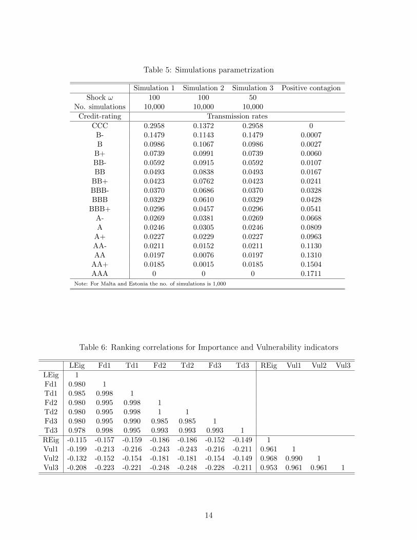
Table 5: Simulations parametrization

Simulation 1 Simulation 2 Simulation 3 Positive contagion

Shock ω 100 100 50No. simulations 10,000 10,000 10,000

Credit-rating Transmission rates

CCC 0.2958 0.1372 0.2958 0B- 0.1479 0.1143 0.1479 0.0007B 0.0986 0.1067 0.0986 0.0027

B+ 0.0739 0.0991 0.0739 0.0060BB- 0.0592 0.0915 0.0592 0.0107BB 0.0493 0.0838 0.0493 0.0167

BB+ 0.0423 0.0762 0.0423 0.0241BBB- 0.0370 0.0686 0.0370 0.0328BBB 0.0329 0.0610 0.0329 0.0428

BBB+ 0.0296 0.0457 0.0296 0.0541A- 0.0269 0.0381 0.0269 0.0668A 0.0246 0.0305 0.0246 0.0809

A+ 0.0227 0.0229 0.0227 0.0963AA- 0.0211 0.0152 0.0211 0.1130AA 0.0197 0.0076 0.0197 0.1310

AA+ 0.0185 0.0015 0.0185 0.1504AAA 0 0 0 0.1711

Note: For Malta and Estonia the no. of simulations is 1,000

Table 6: Ranking correlations for Importance and Vulnerability indicators

LEig Fd1 Td1 Fd2 Td2 Fd3 Td3 REig Vul1 Vul2 Vul3

LEig 1Fd1 0.980 1Td1 0.985 0.998 1Fd2 0.980 0.995 0.998 1Td2 0.980 0.995 0.998 1 1Fd3 0.980 0.995 0.990 0.985 0.985 1Td3 0.978 0.998 0.995 0.993 0.993 0.993 1

REig -0.115 -0.157 -0.159 -0.186 -0.186 -0.152 -0.149 1Vul1 -0.199 -0.213 -0.216 -0.243 -0.243 -0.216 -0.211 0.961 1Vul2 -0.132 -0.152 -0.154 -0.181 -0.181 -0.154 -0.149 0.968 0.990 1Vul3 -0.208 -0.223 -0.221 -0.248 -0.248 -0.228 -0.211 0.953 0.961 0.961 1

14

4 Positive Contagion

“We spoke a lot about contagion whenthings go poorly but I believe there is apositive contagion when things go well. ”

Mario Draghi, summer 2012

4.1 A world of two contagions

In the model analysed up to now, the only possible transition for countries was downwards. Forinstance, in the simple model with only four ratings from subsection 2.2.2, I had:

A→ B → C → D

In reality however, countries can also be upgraded; and as Draghi’s quotation suggests, thesign of contagion is probably determined on a daily basis by market news and sentiments. Anannouncement like the “Draghi Put” or a successful summit might lead to a round of positivecontagion, whereas a failed government bonds auction or the publication of exorbitant youthunemployment rates may induce negative contagion. In this more realistic world of two contagions- positive and negative - the transition pattern becomes:

A� B � C → D

Akin to negative credit spillovers, positive ones occur if institution/sovereign i’s initial upgradeleads to an increase in the upgrade probabilities of its creditors. This section extends the basicdefault model with only four credit ratings to allow for this possibility.

For simplicity, I ignore the exogenous factors that could lead to upgrades and downgrades andconcentrate on credit changes that happen because of credit spillovers. Let ξ(crit) ∈ [0; 1] be therate at which institution i with credit-rating crit transmits a positive spillover to its creditors. Inthis case, the positive transmission rates vector ξ shall be increasing in cr, reflecting the fact that itbecomes easier for an institution to transmit positive spillovers as its rating rises. Since a defaultedorganisation cannot transmit positive spillovers, I further simplify the vector as: ξ(D) = 0, andξ(cr) ∈ (0; 1] for any cr 6= D.

For institution i to be upgraded from B to A thanks to a positive credit spillover from one of itsdebtors j, it must itself have rating B at the outset - which happens with probability bit, one of itsdebtors must have rating crjt ∈{A, B, C} - which happens with probabilities ψjt = {ajt, bjt, cjt}respectively - and transmit the positive spillover at rate ξ(crjt).

In a world of two contagions, the differential equation that describes the probability that i hasrating A at any point in time is therefore:

daidt

= −ω∑j

vij {aitzjt} θ(crjt) + φ∑j

vij {bitψjt} ξ(crjt) (9)

where φ ∈ R+ captures the magnitude of the positive spillovers. Here I assume that both contagionspropagate through the same network - the network of investment shares with adjacency matrixV. A more complex and realistic model would allow positive and negative contagions to spreadthrough multiple and/or different networks.

15

Similarly, the probability that i has rating B increases in i’s probability of being downgradedfrom A to B, decreases in i’s probability of being downgraded from B to C, decreases in i’sprobability of being upgraded from B to A, and increases in i’s probability of being upgraded fromC to B.

dbidt

= ω∑j

vij {aitzjt} θ(crjt)−ω∑j

vij {bitzjt} θ(crjt)−φ∑j

vij {bitψjt} ξ(crjt)+φ∑j

vij {citψjt} ξ(crjt)

(10)Since once defaulted, an institution can no longer be upgraded, the probability that i has rating

C increases in i’s probability of being downgraded from B to C, decreases in i’s probability ofbeing downgraded from C to D, and decreases in i’s probability of being upgraded from C to B:

dcidt

= ω∑j

vij {bitzjt} θ(crjt)− ω∑j

vij {citzjt} θ(crjt)− φ∑j

vij {citψjt} ξ(crjt) (11)

Finally, the probability of defaulting remains as before:

ddidt

= ω∑j

vij {citzjt} θ(crjt) (12)

Note that this is a more general version of the model presented in subsection 2.2.2 where φ -the magnitude of positive spillovers - was equal to zero, i.e. the positive contagion channel wasshut down.5

4.2 Can positive contagion save the Eurozone?

“Where’s your positive contagion now,Mr. Draghi?”

J. Warner, The Telegraph (05/02/2013)

To analyse this more complex model through computer simulations I define:

Pr(i upgraded) = φ∑j

vijξ(crj) (13)

The new extended spillovers’ function in the computer algorithm, now associates to eachcountry i two transmission rates θ(cri) and ξ(cri). After computing country-specific downgradeand upgrade probabilities using equations 7 and 13, some countries are stochastically downgradedand upgraded producing a new vector of ratings.

Whether positive contagion ultimately dominates its negative counterpart will depend both onthe transmission rates vectors ξ and θ, and the respective spillover magnitudes ω and φ. While

5Following my discussion in footnote 4 about how this multi-stage epidemic model might be used in the contextof contagious mental illnesses, note that this extended version with both positive and negative contagions couldallow researchers to investigate in a more systematic way “how depressed people’s well-being is enhanced or erodedby positive and negative social interactions.”(Kashdan & Steger (2009)) Different networks, reflecting the type andintensity of the interaction between people, could be used to propagate the latter.

16

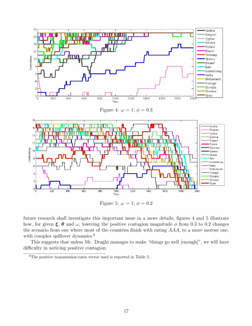
Figure 4: ω = 1; φ = 0.3

Figure 5: ω = 1; φ = 0.2

future research shall investigate this important issue in a more details, figures 4 and 5 illustratehow, for given ξ, θ and ω, lowering the positive contagion magnitude φ from 0.3 to 0.2 changesthe scenario from one where most of the countries finish with rating AAA, to a more morose one,with complex spillover dynamics.6

This suggests that unless Mr. Draghi manages to make “things go well [enough]”, we will havedifficulty in noticing positive contagion.

6The positive transmission-rates vector used is reported in Table 5.

17

5 Conclusion and Future Research

“The deadliest aspect of the Eurozonecrisis is the tripwire linking the riskinessof banks and governments.”

Acharya et al. (2010)

Most of the literature on financial contagion in networks has concentrated on analysing how aninitial default of a bank or country triggers a cascade of further failures. The Eurozone sovereigndebt crisis however has demonstrated that although defaults are likely to be prevented, credit-rating downgrades occur rather often. Since credit-ratings are one of the key drivers of investmentdecisions, a model explaining credit risk spillovers could help understand the observed reallocationof investors’ portfolios in response to changes in the creditworthiness of interlinked countries orbanks. To identify such credit risk spillovers, this paper models the process of default as a multi-stage disease with each credit-rating corresponding to a different infection phase. I use the modelto develop indicators of systemic importance and vulnerability by investigating how the initialexogenous change in the creditworthiness of one of the members of the financial network impactsthe creditworthiness of all the other ones.

The illustration of the model in the context of the Eurozone sovereign debt crisis yields in-teresting and intuitive results. For example, I find that France and Germany occupy the highestpositions in the systemic importance hierarchy. However, the interpretation of all the results isnecessarily limited by the small dataset. Future research should include more countries and testthe model on interbank data, as well as investigate more carefully such phenomena as tippingpoints and contagion waves. The above quote from Acharya et al. (2010) implies that governmentsand banks are closely interlinked. Hence further research should not only analyse the networks ofbanks and governments separately, but also investigate how an initial shock in one of the networkscould potentially engender contagion in the other one, or even change its structure.

The literature has focused almost exclusively on negative contagion. However, policymakersseem to be aware that the same endogenous feedback mechanisms that yield negative financialcontagion, could in principle be used to activate positive spillovers and shift investors’ sentiments.Unfortunately, the extension of the model to include such positive spillovers shows that even thoughpositive contagion could be an attractive solution to the Eurozone sovereign debt crisis, the mainpolicy question remains how to generate it permanently, halting its negative counterpart. Anothertask for further research is therefore to examine how the ratio of positive to negative spillovermagnitudes determines the overall sign of contagion.

References

Acharya, I.D., Schnabl, P., & Viral, V. (2010). A pyrrhic victory? Bank bailouts and sovereigncredit risk. Working paper, NYU-Stern, CEPR Discussion Paper 8679.

Afonso, A. (2003). Understanding the determinants of sovereign debt ratings: Evidence of the twoleading agencies. Journal of Economics and Finance, 27, 56–74.

Allen, F., & Babus, A. (2009). Networks in finance. The Network Challenge, edited by P. Klein-dorfer and J. Wind, Wharton School Publishing, 367–382.

18

Allen, F., & Gale, D. (2000). Financial contagion. Journal of Political Economy, 108, 1–33.

Arezki, R., Candelon, B., & Sy, A.N.R. (2011). Sovereign Rating News and Financial MarketsSpillovers: Evidence from the European Debt Crisis. IMF Working Paper.

Bissoondoyal-Bheenick, E., & Treepongkaruna, S. (2009). An analysis of the determinant of bankratings: Comparison across ratings agencies. JEL Classification: G15.

Caporale, G. M., Serguieva, A., & Wu, H. (2008). Financial contagion: evolutionary optimization ofa multinational agent-based model. Intelligent Systems in Accounting, Finance and Management.Intell. Sys. Acc. Fin. Mgmt, 16, 111–125.

Cheung, S. (1996). Provincial credit ratings in Canada: An ordered probit analysis. Bank ofCanada, Working Paper 96-6.

Corsetti, G., Pesenti, P., & Roubini. N. (1999). Paper tigers? A model of the Asian crisis. EuropeanEconomic Review, 43.

Demiris, N., Kypraios, T., & Smith, L.V. (2014) On the epidemic of financial crises. Journal ofthe Royal Statistical Society: Series A (Statistics in Society), 177, 697–723.

Diamond, D.W., & Dybvig, P.H. (1983). Bank runs, deposit insurance, and liquidity. Journal ofPolitical Economy, 91, 401–419.

Eichengreen, B., Rose, A., & Wyplosz, C. (1996). Contagious currency crises. Scandinavian Journalof Economics.

Elliott, M., Golub, B., & Jackson, M.O. (2014). Financial networks and contagion. AmericanEconomic Review, 104, 3115–3153, doi: 10.1257/aer.104.10.3115

Espinosa-Vega, M., & Sole, J. (2011). Cross-border financial surveillance: A network perspective.Journal of Financial Economic Policy, 3, 182–205.

Farmer, J.D., & Foley, D. (2009). The economy needs agent-based modelling. Nature, 460, 685–686.

Gai, P., Haldane, A., & Kapadia, S. (2011). Complexity, concentration and contagion. Journal ofMonetary Economics, 58, 453–470.

Gerlach, S. & Smets, F. (1995). Contagious speculative attacks. European Journal of PoliticalEconomy, 11, 5–63.

Gladwell, M. (2000). The Tipping Point: How Little Things Can Make a Big Difference. LittleBrown.

Haldane, A. (2009). Rethinking the financial network. Speech delivered at the Financial StudentAssociation, Amsterdam.

Jaquet, V., & Pechal, M. (2009). Epidemic spreading in a social network. ETH Zurich, ProjectReport.

19

Joiner, T.E., & Katz, J. (1999). Contagion of Depressive Symptoms and Mood: Meta-analyticReview and Explanations From Cognitive, Behavioral, and Interpersonal Viewpoints. AmericanPsychological Association, Clinical Psychology: Science and Practice, V6 N2.

Kaminsky, G.L., & Reinhart, C.M. (1998). Financial crises in Asia and Latin America: Then andnow. American Economic Review, 88, 444–448.

Kashdan, T.B., & Steger, M.F. (2009). Depression and Everyday Social Activity, Belonging, andWell-Being. Journal of Counseling Psychology, 56(2), 289–300.

Kermack, W.O., & McKendrick, A.G.(1932). A contribution to the mathematical theory of epi-demics. Proceedings of the Royal Society of London, 83, 138–155.

Masson, P.R., (1999). Multiple equilibria, contagion and the emerging market crises. IMF WorkingPaper.

May, R.M., Levin, S.A., & Sugihara, G. (2008). Complex systems: Ecology for bankers. Nature,451, 893–895.

Melliosa, C., & Paget-Blanc, E. (2006). Which factors determine sovereign credit ratings? Euro-pean Journal of Finance, 12, 361–377.

Newman, M.E.J. (2012). Networks: An Introduction. Oxford University Press.

Pesenti, P. & Tille, C. (2000). The economics of currency crises and contagion: An introduction.FRBNY Economic Policy Review.

Upper, C. (2006). Contagion due to interbank credit exposures: What do we know, why do we knowit, and what should we know? Bank for International Settlements.

Zigrand, J.-P. (2014). Systems and Systemic Risk in Finance and Economics. SRC Special Paper,1.

20