multiple linear regression

An Example for Multiple Linear Regression

- by Ravindra Gokhale

Reference: Montgomery, D., C., and Runger, G., C. Applied Statistics and Probability

for Engineers, Third Edition, John Wiley and Sons, Inc.

The table below (on next page) presents data on taste-testing 38 brands of pinot noir wine (the

data were first reported in an article by Kwan, Kowalski, and Skogenboe in an article in the

Journal of Agricultural and Food Chemistry, Vol. 27, 1979, and it also appears as one of the

default data sets in Minitab software). The response variable is y (that is, “quality”) and we wish

to find the “best” regression equation that relates quality to the other five parameters.

Different aspects of multiple linear regression discussed in class are mentioned in this exercise,

with some additional insights.

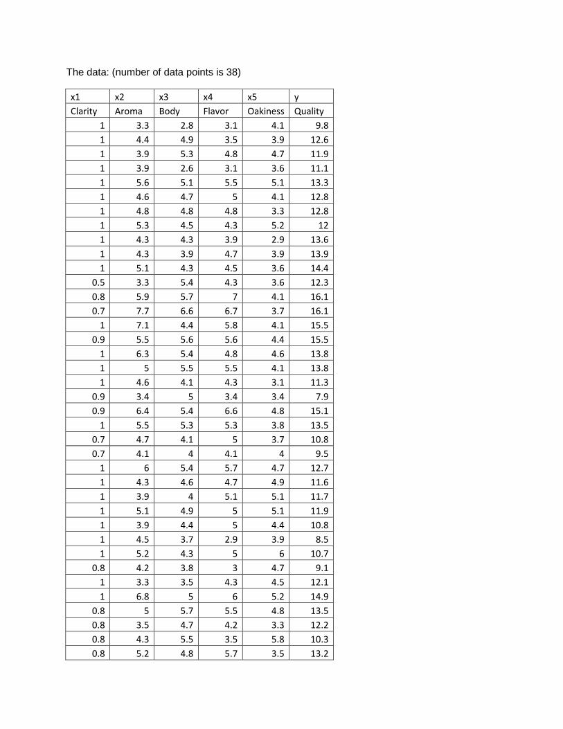
The data: (number of data points is 38)

x1 x2 x3 x4 x5 y

Clarity Aroma Body Flavor Oakiness Quality

1 3.3 2.8 3.1 4.1 9.8

1 4.4 4.9 3.5 3.9 12.6

1 3.9 5.3 4.8 4.7 11.9

1 3.9 2.6 3.1 3.6 11.1

1 5.6 5.1 5.5 5.1 13.3

1 4.6 4.7 5 4.1 12.8

1 4.8 4.8 4.8 3.3 12.8

1 5.3 4.5 4.3 5.2 12

1 4.3 4.3 3.9 2.9 13.6

1 4.3 3.9 4.7 3.9 13.9

1 5.1 4.3 4.5 3.6 14.4

0.5 3.3 5.4 4.3 3.6 12.3

0.8 5.9 5.7 7 4.1 16.1

0.7 7.7 6.6 6.7 3.7 16.1

1 7.1 4.4 5.8 4.1 15.5

0.9 5.5 5.6 5.6 4.4 15.5

1 6.3 5.4 4.8 4.6 13.8

1 5 5.5 5.5 4.1 13.8

1 4.6 4.1 4.3 3.1 11.3

0.9 3.4 5 3.4 3.4 7.9

0.9 6.4 5.4 6.6 4.8 15.1

1 5.5 5.3 5.3 3.8 13.5

0.7 4.7 4.1 5 3.7 10.8

0.7 4.1 4 4.1 4 9.5

1 6 5.4 5.7 4.7 12.7

1 4.3 4.6 4.7 4.9 11.6

1 3.9 4 5.1 5.1 11.7

1 5.1 4.9 5 5.1 11.9

1 3.9 4.4 5 4.4 10.8

1 4.5 3.7 2.9 3.9 8.5

1 5.2 4.3 5 6 10.7

0.8 4.2 3.8 3 4.7 9.1

1 3.3 3.5 4.3 4.5 12.1

1 6.8 5 6 5.2 14.9

0.8 5 5.7 5.5 4.8 13.5

0.8 3.5 4.7 4.2 3.3 12.2

0.8 4.3 5.5 3.5 5.8 10.3

0.8 5.2 4.8 5.7 3.5 13.2

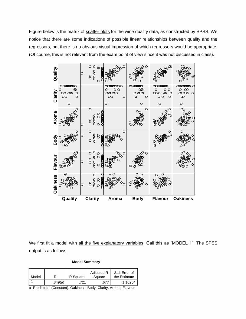
Figure below is the matrix of scatter plots for the wine quality data, as constructed by SPSS. We

notice that there are some indications of possible linear relationships between quality and the

regressors, but there is no obvious visual impression of which regressors would be appropriate.

(Of course, this is not relevant from the exam point of view since it was not discussed in class).

OakinessFlavourBodyAromaClarityQuality

Oak

ine

ss

Fla

vo

ur

Bo

dy

Aro

ma

Cla

rity

Qu

ality

We first fit a model with all the five explanatory variables. Call this as “MODEL 1”. The SPSS

output is as follows:

Model Summary

Model R R Square Adjusted R

Square Std. Error of the Estimate

1 .849(a) .721 .677 1.16254

a Predictors: (Constant), Oakiness, Body, Clarity, Aroma, Flavour

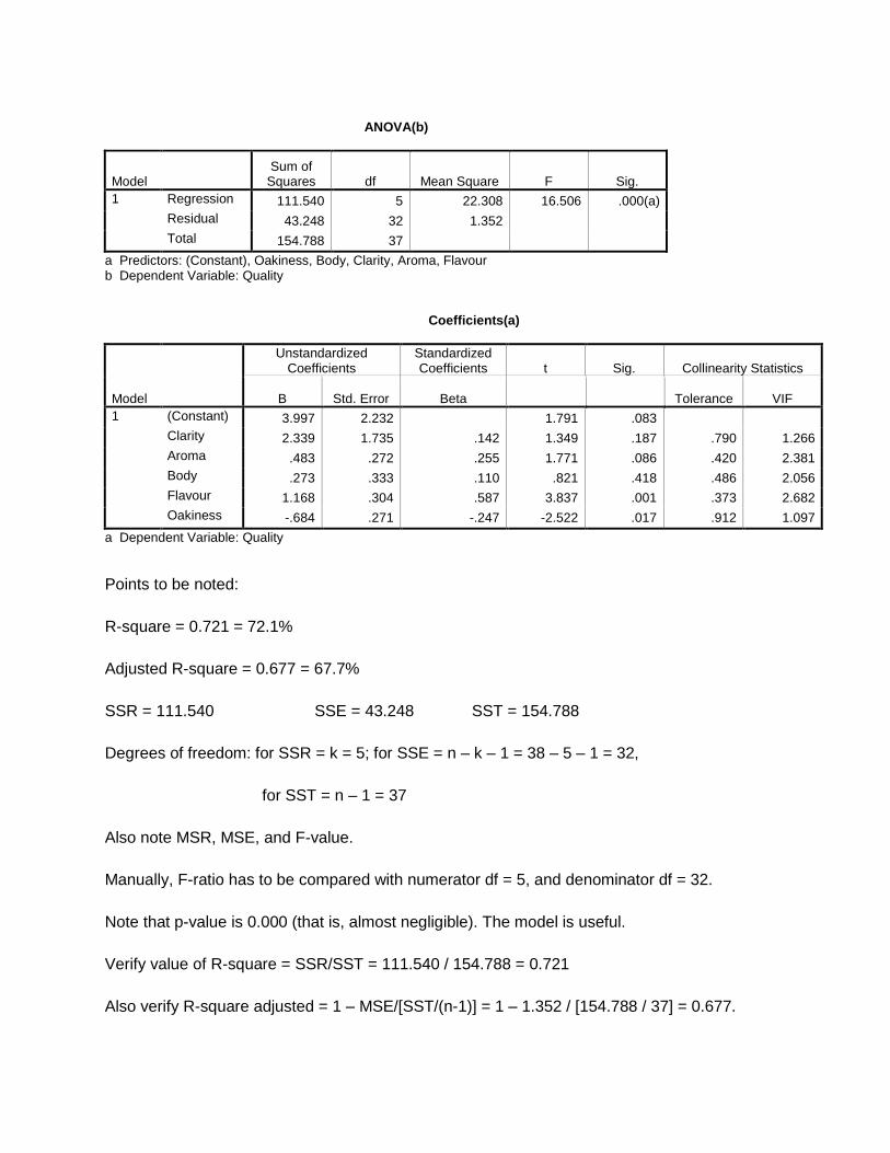
ANOVA(b)

Model Sum of

Squares df Mean Square F Sig.

1 Regression 111.540 5 22.308 16.506 .000(a)

Residual 43.248 32 1.352

Total 154.788 37

a Predictors: (Constant), Oakiness, Body, Clarity, Aroma, Flavour b Dependent Variable: Quality Coefficients(a)

Model

Unstandardized Coefficients

Standardized Coefficients t Sig. Collinearity Statistics

B Std. Error Beta Tolerance VIF

1 (Constant) 3.997 2.232 1.791 .083

Clarity 2.339 1.735 .142 1.349 .187 .790 1.266

Aroma .483 .272 .255 1.771 .086 .420 2.381

Body .273 .333 .110 .821 .418 .486 2.056

Flavour 1.168 .304 .587 3.837 .001 .373 2.682

Oakiness -.684 .271 -.247 -2.522 .017 .912 1.097

a Dependent Variable: Quality

Points to be noted:

R-square = 0.721 = 72.1%

Adjusted R-square = 0.677 = 67.7%

SSR = 111.540 SSE = 43.248 SST = 154.788

Degrees of freedom: for SSR = k = 5; for SSE = n – k – 1 = 38 – 5 – 1 = 32,

for SST = n – 1 = 37

Also note MSR, MSE, and F-value.

Manually, F-ratio has to be compared with numerator df = 5, and denominator df = 32.

Note that p-value is 0.000 (that is, almost negligible). The model is useful.

Verify value of R-square = SSR/SST = 111.540 / 154.788 = 0.721

Also verify R-square adjusted = 1 – MSE/[SST/(n-1)] = 1 – 1.352 / [154.788 / 37] = 0.677.

Although the model is useful and the R-square (and R-square adjusted) is good, the third table

indicates that not all coefficients are significant. For example, “clarity”, “aroma”, and “body” are

not showing significant (p-value > 0.05). Can they be eliminated from the model to form a

simpler model, without compromising much on the R-square?

Also note that the problem of multicollinearity is absent. [An indicator of this is that all VIF values

– as given in the third table are far low than 10]. This is good.

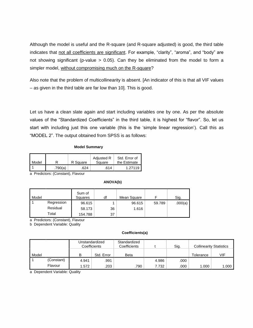
Let us have a clean slate again and start including variables one by one. As per the absolute

values of the “Standardized Coefficients” in the third table, it is highest for “flavor”. So, let us

start with including just this one variable (this is the ‘simple linear regression’). Call this as

“MODEL 2”. The output obtained from SPSS is as follows:

Model Summary



1 .790(a) .624 .614 1.27119

a Predictors: (Constant), Flavour ANOVA(b)

Model Sum of


1 Regression 96.615 1 96.615 59.789 .000(a)

Residual 58.173 36 1.616

Total 154.788 37

a Predictors: (Constant), Flavour b Dependent Variable: Quality Coefficients(a)

Model




1 (Constant) 4.941 .991 4.986 .000

Flavour 1.572 .203 .790 7.732 .000 1.000 1.000


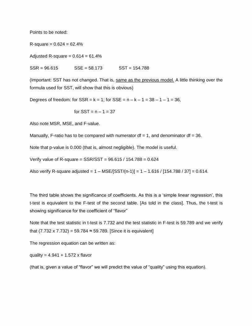
Points to be noted:

R-square = 0.624 = 62.4%

Adjusted R-square = 0.614 = 61.4%

SSR = 96.615 SSE = 58.173 SST = 154.788

(Important: SST has not changed. That is, same as the previous model. A little thinking over the

formula used for SST, will show that this is obvious)

Degrees of freedom: for SSR = k = 1; for SSE = n – k – 1 = 38 – 1 – 1 = 36,

for SST = n – 1 = 37

Also note MSR, MSE, and F-value.

Manually, F-ratio has to be compared with numerator df = 1, and denominator df = 36.

Note that p-value is 0.000 (that is, almost negligible). The model is useful.

Verify value of R-square = SSR/SST = 96.615 / 154.788 = 0.624

Also verify R-square adjusted = 1 – MSE/[SST/(n-1)] = 1 – 1.616 / [154.788 / 37] = 0.614.

The third table shows the significance of coefficients. As this is a ‘simple linear regression’, this

t-test is equivalent to the F-test of the second table. [As told in the class]. Thus, the t-test is

showing significance for the coefficient of “flavor”

Note that the test statistic in t-test is 7.732 and the test statistic in F-test is 59.789 and we verify

that (7.732 x 7.732) = 59.784 ≈ 59.789. [Since it is equivalent]

The regression equation can be written as:

quality = 4.941 + 1.572 x flavor

(that is, given a value of “flavor” we will predict the value of “quality” using this equation).

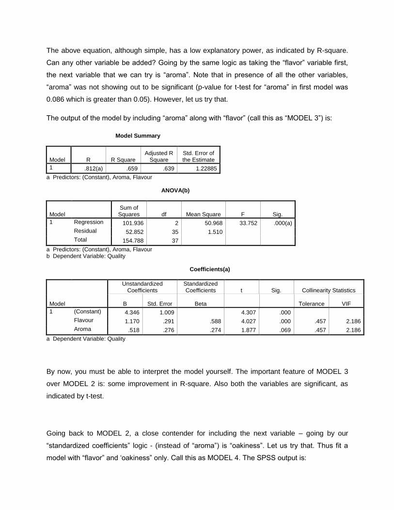
The above equation, although simple, has a low explanatory power, as indicated by R-square.

Can any other variable be added? Going by the same logic as taking the “flavor” variable first,

the next variable that we can try is “aroma”. Note that in presence of all the other variables,

“aroma” was not showing out to be significant (p-value for t-test for “aroma” in first model was

0.086 which is greater than 0.05). However, let us try that.

The output of the model by including “aroma” along with “flavor” (call this as “MODEL 3”) is:

Model Summary



1 .812(a) .659 .639 1.22885

a Predictors: (Constant), Aroma, Flavour ANOVA(b)

Model Sum of


1 Regression 101.936 2 50.968 33.752 .000(a)

Residual 52.852 35 1.510

Total 154.788 37

a Predictors: (Constant), Aroma, Flavour b Dependent Variable: Quality Coefficients(a)

Model




1 (Constant) 4.346 1.009 4.307 .000

Flavour 1.170 .291 .588 4.027 .000 .457 2.186

Aroma .518 .276 .274 1.877 .069 .457 2.186


By now, you must be able to interpret the model yourself. The important feature of MODEL 3

over MODEL 2 is: some improvement in R-square. Also both the variables are significant, as

indicated by t-test.

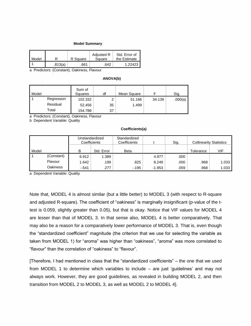
Going back to MODEL 2, a close contender for including the next variable – going by our

“standardized coefficients” logic - (instead of “aroma”) is “oakiness”. Let us try that. Thus fit a

model with “flavor” and ‘oakiness” only. Call this as MODEL 4. The SPSS output is:

Model Summary



1 .813(a) .661 .642 1.22423

a Predictors: (Constant), Oakiness, Flavour ANOVA(b)

Model Sum of


1 Regression 102.332 2 51.166 34.139 .000(a)

Residual 52.456 35 1.499

Total 154.788 37

a Predictors: (Constant), Oakiness, Flavour b Dependent Variable: Quality Coefficients(a)

Model




1 (Constant) 6.912 1.389 4.977 .000

Flavour 1.642 .199 .825 8.249 .000 .968 1.033

Oakiness -.541 .277 -.195 -1.953 .059 .968 1.033


Note that, MODEL 4 is almost similar (but a little better) to MODEL 3 (with respect to R-square

and adjusted R-square). The coefficient of “oakiness” is marginally insignificant (p-value of the t-

test is 0.059, slightly greater than 0.05), but that is okay. Notice that VIF values for MODEL 4

are lesser than that of MODEL 3. In that sense also, MODEL 4 is better comparatively. That

may also be a reason for a comparatively lower performance of MODEL 3. That is, even though

the “standardized coefficient” magnitude (the criterion that we use for selecting the variable as

taken from MODEL 1) for “aroma” was higher than “oakiness”, “aroma” was more correlated to

“flavour” than the correlation of “oakiness” to “flavour”.

[Therefore, I had mentioned in class that the “standardized coefficients” – the one that we used

from MODEL 1 to determine which variables to include – are just ‘guidelines’ and may not

always work. However, they are good guidelines, as revealed in building MODEL 2, and then

transition from MODEL 2 to MODEL 3, as well as MODEL 2 to MODEL 4].

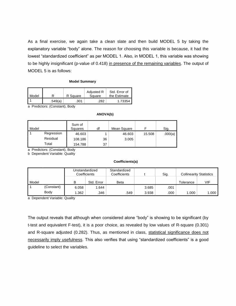
As a final exercise, we again take a clean slate and then build MODEL 5 by taking the

explanatory variable “body” alone. The reason for choosing this variable is because, it had the

lowest “standardized coefficient” as per MODEL 1. Also, in MODEL 1, this variable was showing

to be highly insignificant (p-value of 0.418) in presence of the remaining variables. The output of

MODEL 5 is as follows:

Model Summary



1 .549(a) .301 .282 1.73354

a Predictors: (Constant), Body ANOVA(b)

Model Sum of


1 Regression 46.603 1 46.603 15.508 .000(a)

Residual 108.186 36 3.005

Total 154.788 37

a Predictors: (Constant), Body b Dependent Variable: Quality Coefficients(a)

Model




1 (Constant) 6.058 1.644 3.685 .001

Body 1.362 .346 .549 3.938 .000 1.000 1.000


The output reveals that although when considered alone “body” is showing to be significant (by

t-test and equivalent F-test), it is a poor choice, as revealed by low values of R-square (0.301)

and R-square adjusted (0.282). Thus, as mentioned in class, statistical significance does not

necessarily imply usefulness. This also verifies that using “standardized coefficients” is a good

guideline to select the variables.

However, in real life, while building models using good software, the software will select the best

variables for you. As mentioned in class, choose a model that is simple (that is, as low number

of variables as possible), but does not compromise much on R-square (and R-square adjusted).

Thus one can try many different combinations and finally choose the one that gives the “best

tradeoff” between simplicity and R-square. Moreover, the practical aspects like which variables

are easy from data collection point of view, cost of data collection, etc. will also play an

important role, in real life.

multiple linear regression

Documents