ch06. multiple regression analysis: further issues - hku

Ch06. Multiple Regression Analysis: Further Issues

Ping Yu

HKU Business SchoolThe University of Hong Kong

Ping Yu (HKU) MLR: Further Issues 1 / 39

Effects of Data Scaling on OLS Statistics




Section 2.4a: SLR

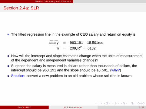
The fitted regression line in the example of CEO salary and return on equity is

\salary = 963.191+18.501roe,

n = 209,R2 = .0132

How will the intercept and slope estimates change when the units of measurementof the dependent and independent variables changes?

Suppose the salary is measured in dollars rather than thousands of dollars, theintercept should be 963,191 and the slope should be 18,501. (why?)

Solution: convert a new problem to an old problem whose solution is known.



A Brute-Force Solution

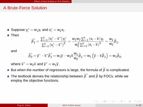
Suppose y�i = w1yi and x�i = w2xi .

Then bβ �1 = ∑ni=1

�x�i �x�

�y�i

∑ni=1

�x�i �x�

�2 =w1w2 ∑n

i=1 (xi �x)yi

w22 ∑n

i=1 (xi �x)2=

w1

w2

bβ 1,

and bβ �0 = y��x�bβ �1 = w1y �w2xw1

w2

bβ 1 = w1

�y �xbβ 1

�= w1

bβ 0,

where x� = w2x and y� = w1y .

But when the number of regressors is large, the formula of bβ is complicated.

The textbook derives the relationship between bβ � and bβ by FOCs, while weemploy the objective functions.



Relationship Between Objective Functions

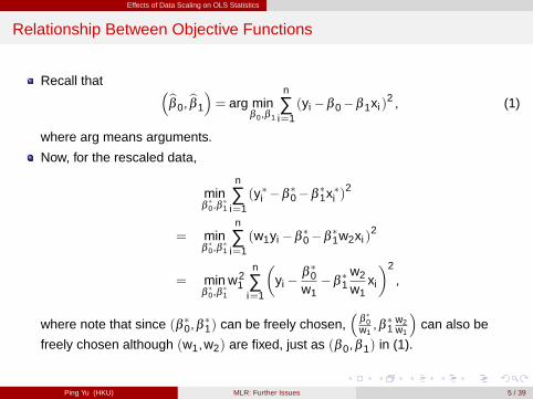
Recall that �bβ 0,bβ 1

�= arg min

β 0,β 1

n

∑i=1(yi �β 0�β 1xi )

2 , (1)

where arg means arguments.

Now, for the rescaled data,

minβ�0,β

�1

n

∑i=1(y�i �β

�0�β

�1x�i )

2

= minβ�0,β

�1

n

∑i=1(w1yi �β

�0�β

�1w2xi )

2

= minβ�0,β

�1

w21

n

∑i=1

�yi �

β�0

w1�β

�1

w2

w1xi

�2

,

where note that since (β �0,β�1) can be freely chosen,

�β�0

w1,β �1

w2w1

�can also be

freely chosen although (w1,w2) are fixed, just as (β 0,β 1) in (1).



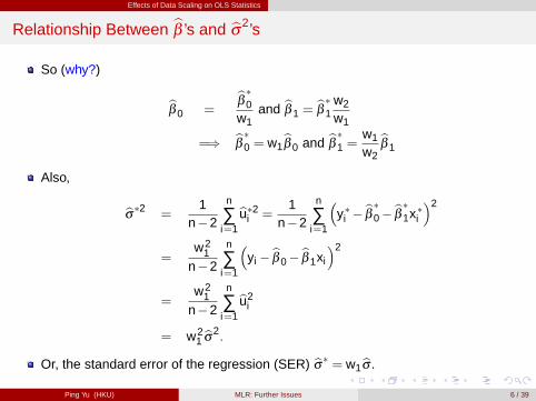
Relationship Between bβ ’s and bσ2’s

So (why?)

bβ 0 =bβ �0w1

and bβ 1 =bβ �1 w2

w1

=) bβ �0 = w1bβ 0 and bβ �1 = w1

w2

bβ 1

Also,

bσ�2 =1

n�2

n

∑i=1

bu�2i =1

n�2

n

∑i=1

�y�i � bβ �0� bβ �1x�i

�2

=w2

1n�2

n

∑i=1

�yi � bβ 0� bβ 1xi

�2

=w2

1n�2

n

∑i=1

bu2i

= w21 bσ2.

Or, the standard error of the regression (SER) bσ� = w1bσ .



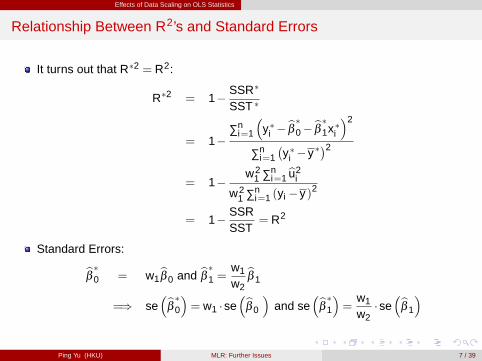
Relationship Between R2’s and Standard Errors

It turns out that R�2 = R2:

R�2 = 1� SSR�

SST �

= 1�∑n

i=1

�y�i � bβ �0� bβ �1x�i

�2

∑ni=1

�y�i �y�

�2

= 1�w2

1 ∑ni=1 bu2

i

w21 ∑n

i=1 (yi �y)2

= 1� SSRSST

= R2

Standard Errors:

bβ �0 = w1bβ 0 and bβ �1 = w1

w2

bβ 1

=) se�bβ �0�= w1 �se

�bβ 0

�and se

�bβ �1�= w1

w2�se

�bβ 1

�



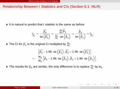
Relationship Between t Statistics and CIs (Section 6.1: MLR)

It is natural to predict that t statistic is the same as before:

tbβ �1 =bβ �1

se�bβ �1� =

w1w2bβ 1

w1w2�se

�bβ 1

� = bβ 1

se�bβ 1

� = tbβ 1.

The CI for β 1 is the original CI multiplied by w1w2

:hbβ �1�1.96 �se�bβ �1� , bβ �1+1.96 �se

�bβ �1�i=

w1

w2

hbβ 1�1.96 �se�bβ 1

�, bβ 1+1.96 �se

�bβ 1

�i.

The results for β 0 are similar; the only difference is to replace w1w2

by w1.



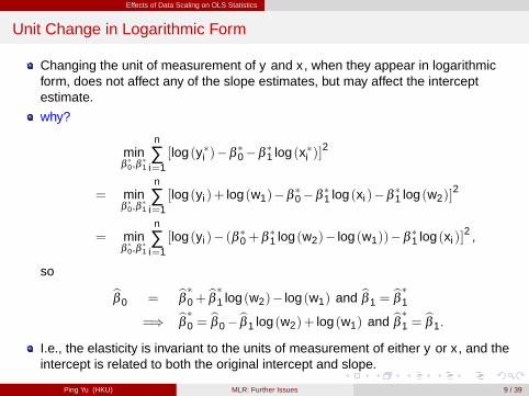
Unit Change in Logarithmic Form

Changing the unit of measurement of y and x , when they appear in logarithmicform, does not affect any of the slope estimates, but may affect the interceptestimate.

why?

minβ�0,β

�1

n

∑i=1[log (y�i )�β

�0�β

�1 log (x�i )]

2

= minβ�0,β

�1

n

∑i=1[log (yi )+ log (w1)�β

�0�β

�1 log (xi )�β

�1 log (w2)]

2

= minβ�0,β

�1

n

∑i=1[log (yi )� (β �0+β

�1 log (w2)� log (w1))�β

�1 log (xi )]

2,

so bβ 0 = bβ �0+ bβ �1 log (w2)� log (w1) and bβ 1 =bβ �1

=) bβ �0 = bβ 0� bβ 1 log (w2)+ log (w1) and bβ �1 = bβ 1.

I.e., the elasticity is invariant to the units of measurement of either y or x , and theintercept is related to both the original intercept and slope.



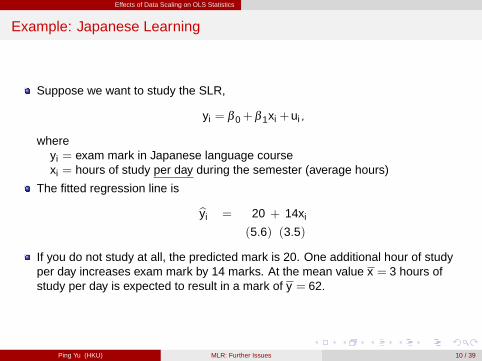
Example: Japanese Learning

Suppose we want to study the SLR,

yi = β 0+β 1xi +ui ,

whereyi = exam mark in Japanese language coursexi = hours of study per day during the semester (average hours)

The fitted regression line is

byi = 20 + 14xi

(5.6) (3.5)

If you do not study at all, the predicted mark is 20. One additional hour of studyper day increases exam mark by 14 marks. At the mean value x = 3 hours ofstudy per day is expected to result in a mark of y = 62.



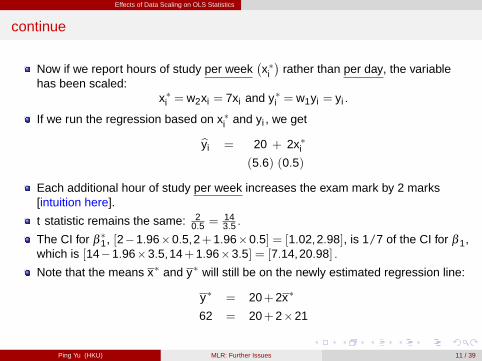
continue

Now if we report hours of study per week�x�i�

rather than per day, the variablehas been scaled:

x�i = w2xi = 7xi and y�i = w1yi = yi .

If we run the regression based on x�i and yi , we get

byi = 20 + 2x�i(5.6) (0.5)

Each additional hour of study per week increases the exam mark by 2 marks[intuition here].

t statistic remains the same: 20.5 =

143.5 .

The CI for β�1, [2�1.96�0.5,2+1.96�0.5] = [1.02,2.98], is 1/7 of the CI for β 1,

which is [14�1.96�3.5,14+1.96�3.5] = [7.14,20.98] .

Note that the means x� and y� will still be on the newly estimated regression line:

y� = 20+2x�

62 = 20+2�21


More on Functional Form




a: More on Using Logarithmic Functional Forms

Logarithmic transformations have the convenient percentage/elasticityinterpretation.

Slope coefficients of logged variables are invariant to rescalings.

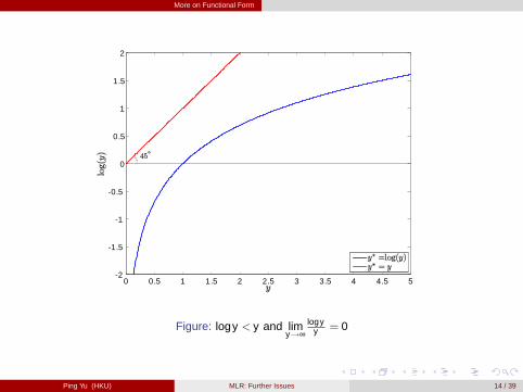
Taking logs often eliminates/mitigates problems with outliers. (why? figure here)

Taking logs often helps to secure normality (e.g., log(wage) vs. wage) andhomoskedasticity (see Chapter 8 for an example).

Variables measured in units such as years (e.g., education, experience, tenure,age, etc) should not be logged.

Variables measured in percentage points (e.g., unemployment rate, participationrate of a pension plan, etc.) should also not be logged.

Logs must not be used if variables take on zero or negative values (e.g., hours ofwork during a month).

It is hard to reverse the log-operation when constructing predictions. (we willdiscuss more on this point later in this chapter)



0 0.5 1 1.5 2 2.5 3 3.5 4 4.5 52

1.5

1

0.5

0

0.5

1

1.5

2

Figure: logy < y and limy!∞

logyy = 0



b: Models with Quadratics

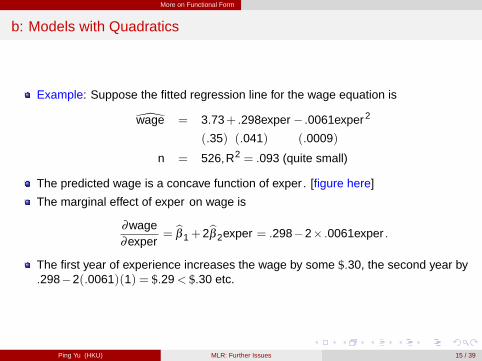
Example: Suppose the fitted regression line for the wage equation is

\wage = 3.73+ .298exper � .0061exper2

(.35) (.041) (.0009)

n = 526,R2 = .093 (quite small)

The predicted wage is a concave function of exper . [figure here]

The marginal effect of exper on wage is

∂wage∂exper

= bβ 1+2bβ 2exper = .298�2� .0061exper .

The first year of experience increases the wage by some $.30, the second year by.298�2(.0061)(1) = $.29< $.30 etc.



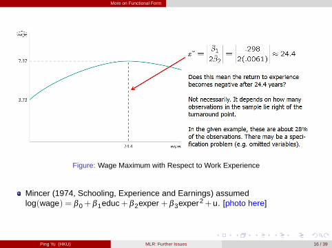
Figure: Wage Maximum with Respect to Work Experience

Mincer (1974, Schooling, Experience and Earnings) assumedlog(wage) = β 0+β 1educ+β 2exper +β 3exper2+u. [photo here]



History of the Wage Equation

Jacob Mincer (1922-2006), Columbia,father of modern labor economics



Example: Effects of Pollution on Housing Prices

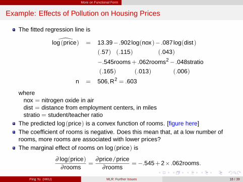
The fitted regression line is

\log (price) = 13.39� .902log(nox)� .087log(dist)

(.57) (.115) (.043)

�.545rooms+ .062rooms2� .048stratio

(.165) (.013) (.006)

n = 506,R2 = .603

wherenox = nitrogen oxide in airdist = distance from employment centers, in milesstratio = student/teacher ratio

The predicted log (price) is a convex function of rooms. [figure here]The coefficient of rooms is negative. Does this mean that, at a low number ofrooms, more rooms are associated with lower prices?The marginal effect of rooms on log (price) is

∂ log(price)∂ rooms

=∂price/price

∂ rooms= �.545+2� .062rooms.



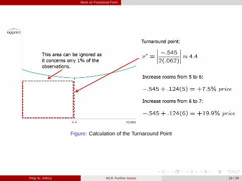
Figure: Calculation of the Turnaround Point



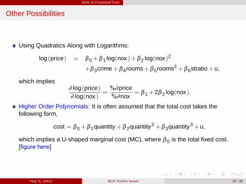
Other Possibilities

Using Quadratics Along with Logarithms:

log (price) = β 0+β 1 log(nox)+β 2 log(nox)2

+β 3crime+β 4rooms+β 5rooms2+β 6stratio+u,

which implies∂ log (price)∂ log(nox)

=%∂price%∂nox

= β 1+2β 2 log(nox).

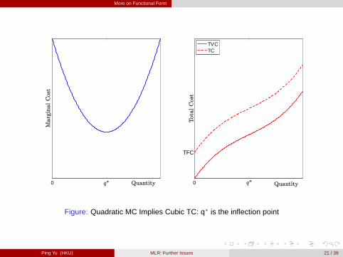
Higher Order Polynomials: It is often assumed that the total cost takes thefollowing form,

cost = β 0+β 1quantity +β 2quantity2+β 3quantity3+u,

which implies a U-shaped marginal cost (MC), where β 0 is the total fixed cost.[figure here]



0 0

TFC

TVCTC

Figure: Quadratic MC Implies Cubic TC: q� is the inflection point



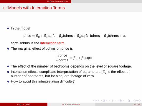
c: Models with Interaction Terms

In the model

price = β 0+β 1sqrft+β 2bdrms+β 3sqrft �bdrms+β 4bthrms+u,

sqrft �bdrms is the interaction term.

The marginal effect of bdrms on price is

∂price∂bdrms

= β 2+β 3sqrft .

The effect of the number of bedrooms depends on the level of square footage.

Interaction effects complicate interpretation of parameters: β 2 is the effect ofnumber of bedrooms, but for a square footage of zero.

How to avoid this interpretation difficulty?



Reparametrization of Interaction Effects

The modely = β 0+β 1x1+β 2x2+β 3x1x2+u

can be reparametrized as

y = α0+ δ 1x1+ δ 2x2+β 3 (x1�µ1) (x2�µ2)+u,

where µ1 = E [x1] and µ2 = E [x2] are population means of x1 and x2, and can bereplaced by their sample means.

What is the relationship between�bα0,

bδ 1,bδ 2

�and

�bβ 0,bβ 1,

bβ 2

�? (Exercise)

Now,∂y∂x2

= δ 2+β 3 (x1�µ1) ,

i.e., δ 2 is the effect of x2 if all other variables take on their mean values.

Advantages of reparametrization:- It is easy to interpret all parameters.- Standard errors for partial effects at the mean values are available.- If necessary, interaction may be centered at other interesting values.


More on Goodness-of-Fit and Selection of Regressors




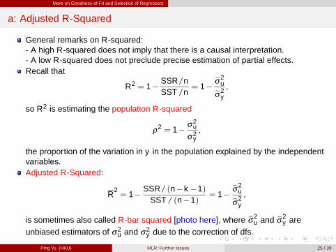
a: Adjusted R-Squared

General remarks on R-squared:- A high R-squared does not imply that there is a causal interpretation.- A low R-squared does not preclude precise estimation of partial effects.Recall that

R2 = 1� SSR/nSST /n

= 1�eσ2

ueσ2y

,

so R2 is estimating the population R-squared

ρ2 = 1� σ2

u

σ2y,

the proportion of the variation in y in the population explained by the independentvariables.Adjusted R-Squared:

R2= 1� SSR/ (n�k �1)

SST / (n�1)= 1�

bσ2ubσ2y

,

is sometimes also called R-bar squared [photo here], where bσ2u and bσ2

y areunbiased estimators of σ2

u and σ2y due to the correction of dfs.



History of R2

Henri Theil (1924-2000)1, Chicago and Florida

1He is a Dutch econometrician. Two other Dutch econometricians, Jan Tinbergen (1903-1994) and TjallingKoopmans (1910-1985) won the Nobel Prize in economics in 1969 and 1975, respectively.



continue

R2

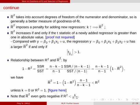
takes into account degrees of freedom of the numerator and denominator, so isgenerally a better measure of goodness-of-fit.

R2

imposes a penalty for adding new regressors: k " =) R2 #

R2

increases if and only if the t statistic of a newly added regressor is greater thanone in absolute value. [proof not required]- Compared with y = β 0+β 1x1+u, the regression y = β 0+β 1x1+β 2x2+u has

a larger R2

if and only if ��tbβ 2

��> 1.

Relationship between R2 and R2: by

1�R2 =SSRSST

=n�k �1

n�1SSR/ (n�k �1)

SST / (n�1)=

n�k �1n�1

�1�R

2�,

we have

R2= 1�

�1�R2

� n�1n�k �1

< R2

unless k = 0 or R2 = 1. [figure here]

Note that R2

even gets negative if R2 < kn�1 .



0 1

0

1

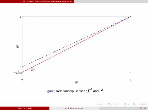
Figure: Relationship Between R2

and R2



b: Using Adjusted R-squared to Choose between Nonnested Models

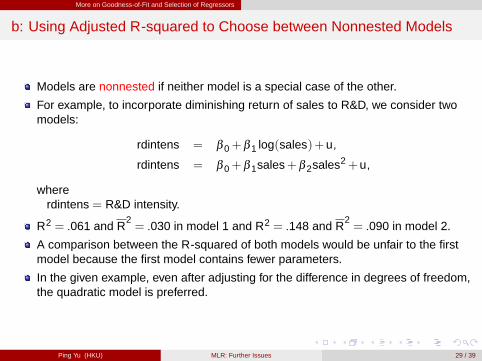
Models are nonnested if neither model is a special case of the other.

For example, to incorporate diminishing return of sales to R&D, we consider twomodels:

rdintens = β 0+β 1 log(sales)+u,

rdintens = β 0+β 1sales+β 2sales2+u,

whererdintens = R&D intensity.

R2 = .061 and R2= .030 in model 1 and R2 = .148 and R

2= .090 in model 2.

A comparison between the R-squared of both models would be unfair to the firstmodel because the first model contains fewer parameters.

In the given example, even after adjusting for the difference in degrees of freedom,the quadratic model is preferred.



Comparing Models with Different Dependent Variables

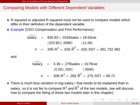
R-squared or adjusted R-squared must not be used to compare models whichdiffer in their definition of the dependent variable.

Example (CEO Compensation and Firm Performance):

\salary = 830.63+ .0163sales+19.63roe

(223.90)(.0089) (11.08)

n = 209,R2 = .029,R2= .020,SST = 391,732,982

and

\lsalary = 4.36+ .275lsales+ .0179roe

(0.29)(.033) (.0040)

n = 209,R2 = .282,R2= .275,SST = 66.72

There is much less variation in log(salary) that needs to be explained than in

salary , so it is not fair to compare R2 and R2

of the two models. (we will discusshow to compare the fitting of these two models later in this chapter)



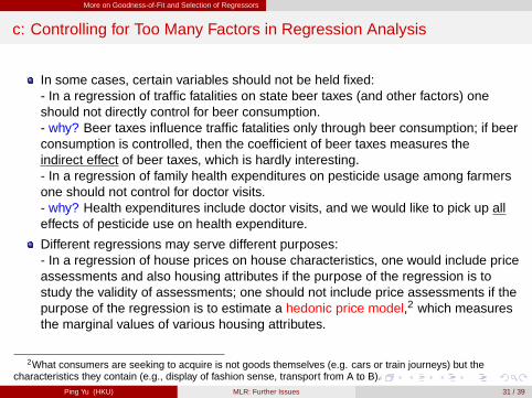
c: Controlling for Too Many Factors in Regression Analysis

In some cases, certain variables should not be held fixed:- In a regression of traffic fatalities on state beer taxes (and other factors) oneshould not directly control for beer consumption.- why? Beer taxes influence traffic fatalities only through beer consumption; if beerconsumption is controlled, then the coefficient of beer taxes measures theindirect effect of beer taxes, which is hardly interesting.- In a regression of family health expenditures on pesticide usage among farmersone should not control for doctor visits.- why? Health expenditures include doctor visits, and we would like to pick up alleffects of pesticide use on health expenditure.

Different regressions may serve different purposes:- In a regression of house prices on house characteristics, one would include priceassessments and also housing attributes if the purpose of the regression is tostudy the validity of assessments; one should not include price assessments if thepurpose of the regression is to estimate a hedonic price model,2 which measuresthe marginal values of various housing attributes.

2What consumers are seeking to acquire is not goods themselves (e.g. cars or train journeys) but thecharacteristics they contain (e.g., display of fashion sense, transport from A to B).



History of Hedonic Price Model

Hedonic Utility: Lancaster, Kelvin J., 1966, A New Approach to Consumer Theory,Journal of Political Economy, 74, 132-157.

Hedonic Pricing: Rosen, S., 1974, Hedonic Prices and Implicit Markets: ProductDifferentiation in Pure Competition, Journal of Political Economy, 82, 34-55.

Kelvin J. Lancaster (1924-1999), Columbia Sherwin Rosen (1938-2001)3, Chicago

3His student Robert H. Thaler (1945-) at the University of Chicago won the Nobel Prize in economics in 2017.Ping Yu (HKU) MLR: Further Issues 32 / 39


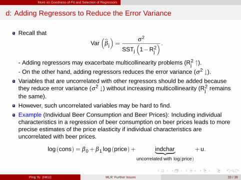
d: Adding Regressors to Reduce the Error Variance

Recall that

Var�bβ j

�=

σ2

SSTj

�1�R2

j

� .- Adding regressors may exacerbate multicollinearity problems (R2

j ").- On the other hand, adding regressors reduces the error variance (σ2 #).Variables that are uncorrelated with other regressors should be added becausethey reduce error variance (σ2 #) without increasing multicollinearity (R2

j remainsthe same).

However, such uncorrelated variables may be hard to find.

Example (Individual Beer Consumption and Beer Prices): Including individualcharacteristics in a regression of beer consumption on beer prices leads to moreprecise estimates of the price elasticity if individual characteristics areuncorrelated with beer prices.

log (cons) = β 0+β 1 log (price)+ indchar| {z }uncorrelated with log(price)

+u.


Prediction and Residual Analysis

(**) Prediction and Residual Analysis



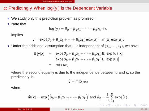
c: Predicting y When log (y) is the Dependent Variable

We study only this prediction problem as promised.

Note thatlog (y) = β 0+β 1x1+ � � �+β k xk +u

impliesy = exp (β 0+β 1x1+ � � �+β k xk )exp (u) =m(x)exp (u) .

Under the additional assumption that u is independent of (x1, � � � ,xk ), we have

E [y jx] = exp (β 0+β 1x1+ � � �+β k xk )E [exp (u) jx]= exp (β 0+β 1x1+ � � �+β k xk )E [exp (u)]

� m(x)α0,

where the second equality is due to the independence between u and x, so thepredicted y is by = bm(x)bα0

where

bm(x) = exp�bβ 0+

bβ 1x1+ � � �+ bβ k xk

�and bα0 =

1n

n

∑i=1

exp (bui ) .



E [exp (u)] � 1

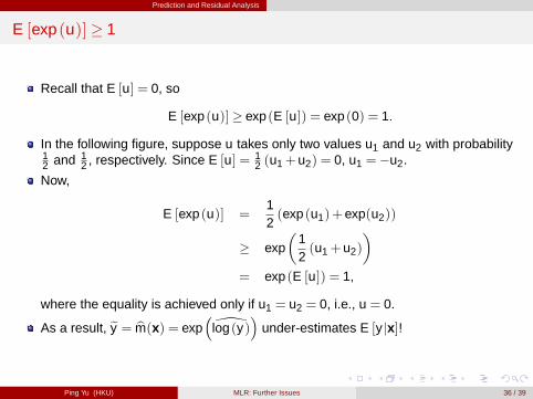
Recall that E [u] = 0, so

E [exp (u)] � exp (E [u]) = exp (0) = 1.

In the following figure, suppose u takes only two values u1 and u2 with probability12 and 1

2 , respectively. Since E [u] = 12 (u1+u2) = 0, u1 = �u2.

Now,

E [exp (u)] =12(exp (u1)+exp(u2))

� exp�

12(u1+u2)

�= exp (E [u]) = 1,

where the equality is achieved only if u1 = u2 = 0, i.e., u = 0.

As a result, ey = bm(x) = exp�\log (y)

�under-estimates E [y jx]!



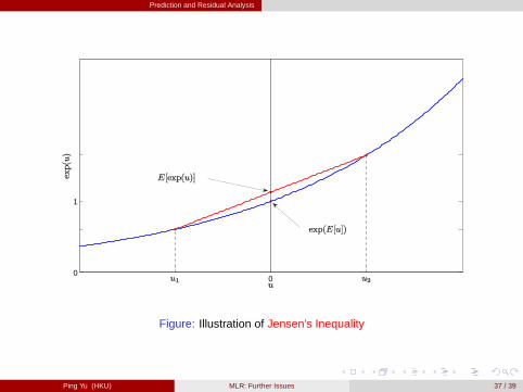
00

1

Figure: Illustration of Jensen’s Inequality



Comparing R-Squared of a Logged and an Unlogged Specification

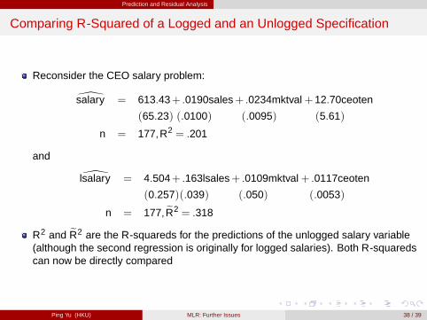
Reconsider the CEO salary problem:

\salary = 613.43+ .0190sales+ .0234mktval+12.70ceoten

(65.23) (.0100) (.0095) (5.61)

n = 177,R2 = .201

and

\lsalary = 4.504+ .163lsales+ .0109mktval+ .0117ceoten

(0.257)(.039) (.050) (.0053)

n = 177, eR2 = .318

R2 and eR2 are the R-squareds for the predictions of the unlogged salary variable(although the second regression is originally for logged salaries). Both R-squaredscan now be directly compared



About eR2

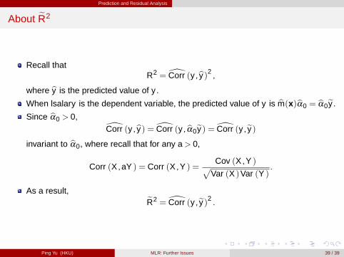
Recall thatR2 =[Corr (y ,by)2 ,

where by is the predicted value of y .

When lsalary is the dependent variable, the predicted value of y is bm(x)bα0 = bα0ey .

Since bα0 > 0,[Corr (y ,by) =[Corr (y , bα0ey) =[Corr (y ,ey)

invariant to bα0, where recall that for any a> 0,

Corr (X ,aY ) = Corr (X ,Y ) =Cov (X ,Y )p

Var (X )Var (Y ).

As a result, eR2 =[Corr (y ,ey)2 .


ch06. multiple regression analysis: further issues - hku

Documents