Transportation Research Part B 149 (2021) 100–117

Contents lists available at ScienceDirect

Transportation Research Part B

journal homepage: www.elsevier.com/locate/trb

A Continuum model for pedestrian flow with explicit

consideration of crowd force and panic effects

Haoyang Liang

a , Jie Du

b , c , S.C. Wong

a , d , ∗

a Department of Civil Engineering, The University of Hong Kong, Hong Kong, China b Yau Mathematical Sciences Center, Tsinghua University, Beijing 10 0 084, China c Yanqi Lake Beijing Institute of Mathematical Sciences and Applications, Beijing 101408, China d Guangdong - Hong Kong - Macau Joint Laboratory for Smart Cities

a r t i c l e i n f o

Article history:

Received 24 December 2020

Revised 16 April 2021

Accepted 4 May 2021

Keywords:

Pedestrian flow

Higher-order traffic model

Crowd force

Numerical solution

a b s t r a c t

This paper proposes a second-order pedestrian model that comprises two types of equa-

tions: continuity equation and a set of transport equations. To complete the model, we

develop Eikonal equations to explicitly consider the effects of the collective decisions of

individuals and crowd pressure on pedestrian dynamics. Then, the crowd movement is

simulated using a set of partial differential equations under appropriate initial and bound-

ary conditions. Based on the stability requirements derived by performing a standard linear

stability analysis, suitable parameters are selected to test the model in a numerical exam-

ple. The proposed second-order system is then solved using the characteristic-wise third-

order weighted essentially non-oscillatory (WENO3) scheme, and the Eikonal equations are

solved using the fast sweeping method. The numerical results indicate the effectiveness of

the model because the derived local flow-density relationship produces a second peak in

the high-density region, which is consistent with previous empirical studies. Besides, the

applicability of the model to an unstable condition is verified through the simulation of

complex phenomena such as stop-and-go waves. Furthermore, the estimate of crowd pres-

sure in the simulation results can be used as a risk-level indicator for crowd management

and control.

© 2021 The Author(s). Published by Elsevier Ltd.

This is an open access article under the CC BY-NC-ND license

( http://creativecommons.org/licenses/by-nc-nd/4.0/ )

1. Introduction

Crowd disasters cause hundreds of deaths worldwide annually. The high numbers of fatalities due to such disasters

and the concomitant negative social effects have attracted significant research attention. Crowd force plays a significant

role in crowd dynamics. In an experimental study, the maximum measured force generated by an individual ranged from

162 N for a fit young female adult to 600 N for a super-fit young male adult ( Dickie and Wanless, 1993 ). However, in

real crowd disasters, force chains can be formed in dense crowds owing to inadvertent physical interactions between peo-

ple, and these chains can induce large variations in crowd pressure, making it almost impossible to control the crowd

( Helbing and Mukerji, 2012 ). According to an estimate obtained in a forensic study, the magnitude of such forces can reach

∗ Corresponding author.

E-mail addresses: lianghy@hku.hk (H. Liang), jdu@tsinghua.edu.cn (J. Du), hhecwsc@hku.hk (S.C. Wong).

https://doi.org/10.1016/j.trb.2021.05.006

0191-2615/© 2021 The Author(s). Published by Elsevier Ltd. This is an open access article under the CC BY-NC-ND license

( http://creativecommons.org/licenses/by-nc-nd/4.0/ )

H. Liang, J. Du and S.C. Wong Transportation Research Part B 149 (2021) 100–117

60 0 0 N ( Hopkins et al., 1993 ), which is considerably greater than the comfortable force level for human beings ( Smith and

Lim, 1995 ). Moreover, according to medical bone fracture analysis, such forces are sufficient to break the ribs of a human,

which may cause suffocation and death ( Keating, 1982 , Fruin, 1993 ). Although the significance of crowd force has been re-

vealed in these empirical studies, most studies of crowd-control methods only considered the number of pedestrians in a

certain area or pedestrian density because of the difficulty to directly measure the mechanical forces generated by moving

crowds ( Zhan et al., 2008 , Bauer et al., 2007 ). The information provided by density distribution is inadequate to describe

the complex states of moving crowds, especially under high-density conditions, when crowd force increases rapidly with in-

creasing density. In addition, as suggested by Moussaïd et al., (2011) , physical interactions have a dominant effect on crowd

movement under high crowd densities.

An increasing number of model-based studies are using new variables to quantitively study crowd force. Social force

models and discrete element models have been developed with reference to traditional agent-based models to determine

the exact value of contact force ( Helbing et al., 20 0 0 , Langston et al., 2006 ). These models quantify the physical and psy-

chological interactions between pedestrians from a microscopic perspective. The physical contact forces determined in such

studies can describe a number of characteristics of real contact forces. For example, according to the results of an evacua-

tion simulation, crowd forces propagate and accumulate within a crowd, reaching an extremely high level at the exit from

a given area ( Lu, 2007 , Lin et al., 2017 ). These results are consistent with the findings of an analysis of the Love Parade dis-

aster ( Helbing and Mukerji, 2012 ). The simulation results of a heuristics-based contact force model also reveal that at high

densities, physical interactions, rather than individual intentions, play the dominant role ( Moussaïd et al., 2011 ). Another

model-based method involves defining crowd force in a GK (Gas-Kinetic) way. Helbing et al., (2007) defined crowd pressure

as the product of local density and local velocity variance, and although this variable is different from mechanical crowd

pressure, they suggested that a monotonously increasing functional relationship exists between the two variables. By using

video analysis, this GK variable can be measured and monitored to forecast crowd disasters and implement appropriate

crowd-control measures ( Helbing and Johansson, 2009 ). In a more complex case, Karamouzas et al., (2014) introduced the

idea of interaction energy through a novel statistical-mechanical approach and naturally defined crowd force as the spa-

tial gradient of energy. Such kinetic-theory-based definitions can quantitatively reflect actual crowd pressure. However, few

studies have evaluated crowd force from a macroscopic perspective owing to the difficulty of parameter calibration.

Whereas microscopic models for pedestrians are based on individual interactions, macroscopic models focus on the col-

lective and average behavior, neglect the detailed interactions between individual pedestrians, and enable analytical anal-

yses (e.g., linear stability analysis) of key parameters in the model, which helps to provide a better understanding of the

characteristics and evolution of pedestrian flow dynamics. Moreover, they save considerable computation time in the case

of crowd simulation under high-density conditions ( Cao et al., 2015 ). Therefore, macroscopic models can quickly iden-

tify a high-density or high-risk area, and can more efficiently describe the high-density crowd dynamics at the aggre-

gate level. The existing macroscopic models can be divided into two classes: first- and higher-order traffic models. The

2D Lighthill–Whitham–Richards (LWR) model, a first-order method, is well-known for its simplicity and effectiveness in

simulating pedestrian movement under low-density conditions ( Hughes, 2002 , Huang et al., 2009 ). However, the simple

speed-density relationship assumed from the fundamental diagram of the LWR model is unrealistic, and the model fails to

describe some qualities of crowd movements, such as non-equilibrium phase transitions ( Johansson et al., 2008 ). Therefore,

higher-order traffic models have been applied to crowd dynamics, including the commonly used 2D Payne–Whitham (PW)

model ( Payne, 1971 , Jiang et al., 2010 ) and Aw–Rascle (AR) model ( Aw and Rascle, 20 0 0 , Zhao et al., 2019 ). Although the

ability of the PW model to simulate vehicular flow has been criticized because of its isotropic property, it can be applied

to simulate crowd movements, which are closer to isotropic properties. Recent research has demonstrated that the 2D PW

model can reproduce complex crowd dynamics, such as the stop-and-go waves ( Twarogowska et al., 2014 , Jiang et al., 2016 ).

However, it still fails to describe the property of crowd pressure. Besides, the force chains cannot be identified in the de-

scription of anticipation pressure terms, which makes the crowd pressure results obtained from these models less reliable.

Moreover, no existing macroscopic model can derive a second peak of the flow-density relationship in high-density regions,

which is a phenomenon that has been observed in crowd movements by Helbing et al., (2007) .

Herein, we propose a second-order model to describe pedestrian movement by using a continuum modeling technique

in which we explicitly consider the effects of pushing force and high density. The pressure term in the 2D PW model is

divided into two components, namely traffic pressure and pushing pressure, which accounts for the propagation property

of pushing pressure. Subsequently, the problem of crowd movement simulation is formulated as a set of partial differential

equations (PDEs) with appropriate initial and boundary conditions. Many numerical algorithms can be applied to solve the

model. In this study, we apply the characteristic-wise WENO3 (Third-Order Weighted Essentially Non-Oscillatory) scheme

( Ren and Zhang, 2003 ) in conjunction with the third-order TVD (Total Variation Diminishing) Runge–Kutta method to solve

the proposed second-order model. This algorithm can ensure the stability of the higher-order traffic model. Moreover, the

Eikonal-type equations in the system can be effectively solved by using the third-order fast sweeping method. The numerical

solutions are applied to the designed evacuation cases, in which we compare the simulation results obtained in the normal

evacuation case with those obtained in the panic evacuation case. The properties and effects of the pushing force due to

the panic sentiment are subsequently revealed. By demonstrating the relationship between experimentally obtained the

average local flow and average local density, we also show that the model reproduces the second peak of the flow–density

relationship in high-density regions, as observed in some empirical studies ( Helbing et al., 2007 , Johansson et al., 2008 ).

101

H. Liang, J. Du and S.C. Wong Transportation Research Part B 149 (2021) 100–117

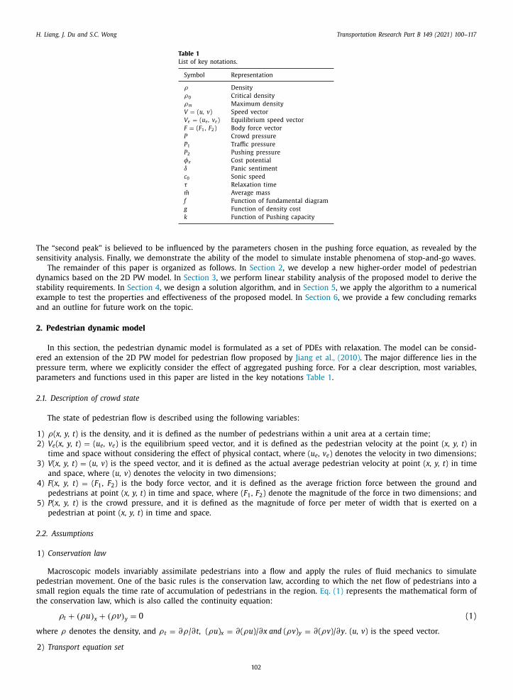
Table 1

List of key notations.

Symbol Representation

ρ Density

ρ0 Critical density

ρm Maximum density

V = ( u, v ) Speed vector

V e = ( u e , v e ) Equilibrium speed vector

F = ( F 1 , F 2 ) Body force vector

P Crowd pressure

P 1 Traffic pressure

P 2 Pushing pressure

φe Cost potential

δ Panic sentiment

c 0 Sonic speed

τ Relaxation time

m Average mass

f Function of fundamental diagram

g Function of density cost

k Function of Pushing capacity

The “second peak” is believed to be influenced by the parameters chosen in the pushing force equation, as revealed by the

sensitivity analysis. Finally, we demonstrate the ability of the model to simulate instable phenomena of stop-and-go waves.

The remainder of this paper is organized as follows. In Section 2 , we develop a new higher-order model of pedestrian

dynamics based on the 2D PW model. In Section 3 , we perform linear stability analysis of the proposed model to derive the

stability requirements. In Section 4 , we design a solution algorithm, and in Section 5 , we apply the algorithm to a numerical

example to test the properties and effectiveness of the proposed model. In Section 6 , we provide a few concluding remarks

and an outline for future work on the topic.

2. Pedestrian dynamic model

In this section, the pedestrian dynamic model is formulated as a set of PDEs with relaxation. The model can be consid-

ered an extension of the 2D PW model for pedestrian flow proposed by Jiang et al., (2010) . The major difference lies in the

pressure term, where we explicitly consider the effect of aggregated pushing force. For a clear description, most variables,

parameters and functions used in this paper are listed in the key notations Table 1 .

2.1. Description of crowd state

The state of pedestrian flow is described using the following variables:

1) ρ( x, y, t ) is the density, and it is defined as the number of pedestrians within a unit area at a certain time;

2) V e ( x, y, t ) = ( u e , v e ) is the equilibrium speed vector, and it is defined as the pedestrian velocity at the point ( x, y, t ) in

time and space without considering the effect of physical contact, where ( u e , v e ) denotes the velocity in two dimensions;

3) V ( x, y, t ) = ( u, v ) is the speed vector, and it is defined as the actual average pedestrian velocity at point ( x, y, t ) in time

and space, where ( u, v ) denotes the velocity in two dimensions;

4) F ( x, y, t ) = ( F 1 , F 2 ) is the body force vector, and it is defined as the average friction force between the ground and

pedestrians at point ( x, y, t ) in time and space, where ( F 1 , F 2 ) denote the magnitude of the force in two dimensions; and

5) P ( x, y, t ) is the crowd pressure, and it is defined as the magnitude of force per meter of width that is exerted on a

pedestrian at point ( x, y, t ) in time and space.

2.2. Assumptions

1) Conservation law

Macroscopic models invariably assimilate pedestrians into a flow and apply the rules of fluid mechanics to simulate

pedestrian movement. One of the basic rules is the conservation law, according to which the net flow of pedestrians into a

small region equals the time rate of accumulation of pedestrians in the region. Eq. (1) represents the mathematical form of

the conservation law, which is also called the continuity equation:

ρt + ( ρu ) x + ( ρv ) y = 0 (1)

where ρ denotes the density, and ρt = ∂ ρ/ ∂ t , ( ρu ) x = ∂ ( ρu )/ ∂ x and ( ρv ) y = ∂ ( ρv )/ ∂ y . ( u, v ) is the speed vector.

2) Transport equation set

102

H. Liang, J. Du and S.C. Wong Transportation Research Part B 149 (2021) 100–117

Another rule of fluid mechanics used in the model is Newton’s law of momentum conservation, which states that the rate

of change of momentum of a material volume is equal to the total force acting on the volume. This law can be expressed

mathematically as follows ( Eq. (2) ):

( ρu ) t +

(ρuu − σxx

m

)x +

(ρu v − τyx

m

)y

=

F 1 m

(2a)

( ρv ) t +

(ρu v − τxy

m

)x +

(ρvv − σyy

m

)y

=

F 2 m

(2b)

where m is the average mass of a pedestrian, which is considered a constant parameter in the model. [ σxx τxy

τyx σyy ] denotes

the stress tensor of the pedestrian flow, as specified in the rules of fluid mechanics. ( F 1 , F 2 ) denotes the body force vector.

The above continuity and transport equation set provide useful relationships between pedestrian dynamics with accu-

rate physical significance, but they are not sufficient to derive mathematical solutions. Therefore, we make the following

assumptions to formulate the complete model.

Assumption 1. The friction force between pedestrians is neglected in the model. As claimed by Hughes (2002) , the shear

force terms depend strongly on their parameterization and they are likely to be small in practice, as they did not dampen

the waves observed by Bradley (1993) . Under such circumstances, this term has been neglected in many continuum models

( Hughes, 2002 , Jiang et al., 2010 , Twarogowska et al., 2014 ). Especially for uni-directional models, where the interaction

between pedestrians is much less than multi-directional cases. Therefore, the proposed model neglects the friction force.

Then, the stress tensor can be simply given by Eq. (3) . [σxx τxy

τyx σyy

]=

[−P 0

0 −P

](3)

where P denotes the crowd pressure.

Assumption 2. The magnitude of equilibrium state speed is determined solely by the density of the surrounding pedestrian

flow ( Eq. (4) ). This feature is based on several observations ( Helbing et al., 2007 , Wong et al., 2010 ) and is widely used in

existing macroscopic models. √

u

2 e + v 2 e = f ( ρ) (4)

where ( u e ,v e ) denotes the equilibrium speed vector, and f ( ρ) indicates the relationship between equilibrium speed and

density.

Assumption 3. The speed direction in the equilibrium state is determined from a psychological perspective. Pedestrians

expect to be able to minimize their estimated travel times but temper this behavior to avoid extremely high densities. This

tempering is assumed to be “separable,” such that pedestrians minimize the summation of their travel time and a function

of the density. Thus, we can derive Eqs. (5) and (6) .

‖

∇ φe ‖

= g ( ρ) + 1 / √

u

2 e + v 2 e (5)

where φe denotes the cost potential ‖ ∇ φe ‖ =

√

( ∂ φe

∂x )

2 + ( ∂ φe

∂y )

2 . g ( ρ) denotes the cost due to high density, and

1 / √

u 2 e + v 2 e is the local travel time.

( u e , v e ) // − ∇ φe (6)

where ∇ φe = ( ∂ φe

∂x ,

∂ φe

∂y ) , ’’//" means parallel to.

Pedestrian behavior can be strongly influenced by geometric conditions: for example, Zhang et al., (2013) observed dur-

ing a real mass event that pedestrians preferred to walk along the boundary of an area. Nonetheless, the above simple

assumption regarding the route-choice strategy is still highly applicable and efficient in simulations of the common walking

preference of pedestrians ( Hughes, 2002 ). Additionally, the given Eikonal-type equation allows one to efficiently obtain a

solution in numerical cases.

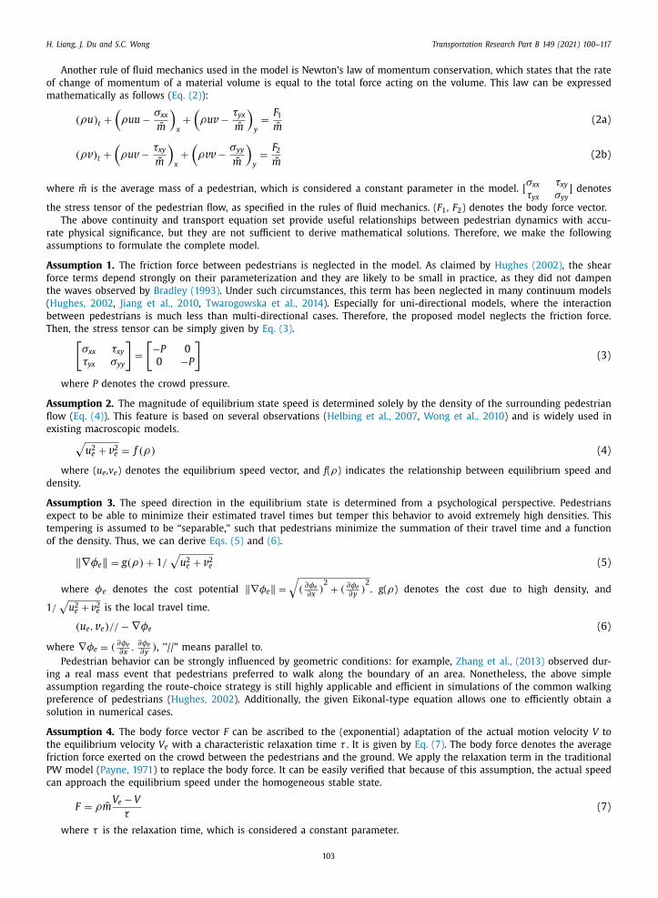
Assumption 4. The body force vector F can be ascribed to the (exponential) adaptation of the actual motion velocity V to

the equilibrium velocity V e with a characteristic relaxation time τ . It is given by Eq. (7) . The body force denotes the average

friction force exerted on the crowd between the pedestrians and the ground. We apply the relaxation term in the traditional

PW model ( Payne, 1971 ) to replace the body force. It can be easily verified that because of this assumption, the actual speed

can approach the equilibrium speed under the homogeneous stable state.

F = ρm

V e − V

τ(7)

where τ is the relaxation time, which is considered a constant parameter.

103

H. Liang, J. Du and S.C. Wong Transportation Research Part B 149 (2021) 100–117

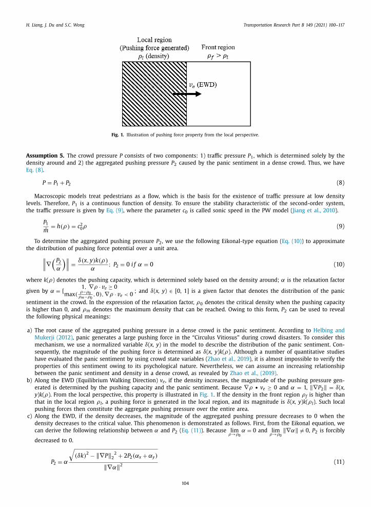
Fig. 1. Illustration of pushing force property from the local perspective.

Assumption 5. The crowd pressure P consists of two components: 1) traffic pressure P 1 , which is determined solely by the

density around and 2) the aggregated pushing pressure P 2 caused by the panic sentiment in a dense crowd. Thus, we have

Eq. (8) .

P = P 1 + P 2 (8)

Macroscopic models treat pedestrians as a flow, which is the basis for the existence of traffic pressure at low density

levels. Therefore, P 1 is a continuous function of density. To ensure the stability characteristic of the second-order system,

the traffic pressure is given by Eq. (9) , where the parameter c 0 is called sonic speed in the PW model ( Jiang et al., 2010 ).

P 1 m

= h ( ρ) = c 2 0 ρ (9)

To determine the aggregated pushing pressure P 2 , we use the following Eikonal-type equation ( Eq. (10) ) to approximate

the distribution of pushing force potential over a unit area. ∥∥∥∇

(P 2 α

)∥∥∥ =

δ( x, y ) k ( ρ)

α; P 2 = 0 i f α = 0 (10)

where k ( ρ) denotes the pushing capacity, which is determined solely based on the density around; α is the relaxation factor

given by α = { 1 , ∇ρ · v e ≥ 0

max ( ρ−ρ0 ρm −ρ0

, 0 ) , ∇ρ · v e < 0 ; and δ( x, y ) ∈ [0, 1] is a given factor that denotes the distribution of the panic

sentiment in the crowd. In the expression of the relaxation factor, ρ0 denotes the critical density when the pushing capacity

is higher than 0, and ρm

denotes the maximum density that can be reached. Owing to this form, P 2 can be used to reveal

the following physical meanings:

a) The root cause of the aggregated pushing pressure in a dense crowd is the panic sentiment. According to Helbing and

Mukerji (2012) , panic generates a large pushing force in the “Circulus Vitiosus” during crowd disasters. To consider this

mechanism, we use a normalized variable δ( x, y ) in the model to describe the distribution of the panic sentiment. Con-

sequently, the magnitude of the pushing force is determined as δ( x, y ) k ( ρ). Although a number of quantitative studies

have evaluated the panic sentiment by using crowd state variables ( Zhao et al., 2019 ), it is almost impossible to verify the

properties of this sentiment owing to its psychological nature. Nevertheless, we can assume an increasing relationship

between the panic sentiment and density in a dense crowd, as revealed by Zhao et al., (2019) .

b) Along the EWD (Equilibrium Walking Direction) v e , if the density increases, the magnitude of the pushing pressure gen-

erated is determined by the pushing capacity and the panic sentiment. Because ∇ρ • v e ≥ 0 and α = 1, ‖∇P 2 ‖ = δ( x,

y ) k ( ρ). From the local perspective, this property is illustrated in Fig. 1 . If the density in the front region ρ f is higher than

that in the local region ρ l , a pushing force is generated in the local region, and its magnitude is δ( x, y ) k ( ρ l ). Such local

pushing forces then constitute the aggregate pushing pressure over the entire area.

c) Along the EWD, if the density decreases, the magnitude of the aggregated pushing pressure decreases to 0 when the

density decreases to the critical value. This phenomenon is demonstrated as follows. First, from the Eikonal equation, we

can derive the following relationship between α and P 2 ( Eq. (11) ). Because lim

ρ→ ρ0

α = 0 and lim

ρ→ ρ0

‖ ∇α‖ � = 0 , P 2 is forcibly

decreased to 0.

P 2 = α

√

( δk ) 2 − ‖ ∇P ‖ 2

2 + 2 P 2 ( αx + αy )

2 (11)

‖ ∇α‖

104

H. Liang, J. Du and S.C. Wong Transportation Research Part B 149 (2021) 100–117

V

2.3. Mathematical model

To summarize, the proposed model considers two factors that significantly influence pedestrian movement. The first

is individual attention, which dominates pedestrians’ movement characteristics under low-density conditions. The second is

crowd pressure, which dominates crowd dynamics under high-density conditions. Crowd pressure provides extra momentum

to the initial speed, which is defined by the equilibrium speed. The final PDE system includes the following equations:

1) Continuity equation:

ρt + ( ρu ) x + ( ρv ) y = 0 (12)

2) Transport equation set: {( ρu ) t +

(ρu

2 + h ( ρ) )

x + ( ρu v ) y = ρ u e −u

τ − 1 m

∂ P 2 ∂x

( ρv ) t + ( ρu v ) x +

(ρv 2 + h ( ρ)

)y

= ρ v e −v τ − 1

m

∂ P 2 ∂y

(13)

3) Fundamental diagram: √

u

2 e + v 2 e = f ( ρ) (14)

4) Route-choice strategy along the equilibrium speed direction: {‖

∇ φe ‖

= g ( ρ) + 1 / f ( ρ) ( u e , v e ) // − ∇ φe

(15)

5) Pushing pressure equation: ∥∥∥∇

(P 2 α

)∥∥∥ =

δ( x, y ) k ( ρ)

α; P 2 = 0 i f α = 0 (16)

3. Linear stability analysis

In this section, we perform a linear stability analysis to derive the requirements for traffic stability.

First, we eliminate the continuity equation terms ( Eq. (12) ) in the transport equation set ( Eq. (13) ) and write the conser-

vation PDEs in the following form ( Eq. (17) ): {ρt + ∇ · ( ρV ) = 0

V t + ( V · ∇ ) V + h

′ ( ρ) ∇ρρ =

−→

V ep −V

τ

(17)

where −→

V ep = V e − τ � p

ρm

, which is defined as the equilibrium speed vector considering the effect of the aggregate pushing force. −→

ep is determined by using the density because both the equilibrium speed vector and the aggregate pushing force depend

on the density distribution.

To analyze the linear stability properties of the model, we assume that ( ρ , V ) = ( ρ0 , V 0 ) are the steady-state solutions

of the conservation equation. In the steady state, −→

V ep = V 0 .

Then, the variations are defined as ⎧ ⎨

⎩

δρ = ρ( x, y, t ) − ρ0

δV = V ( x, y, t ) − V 0

δ(−→

V ep

)=

−→

V ep ( ρ) − V 0

(18)

By substituting the permutations into the conservation PDEs and ignoring the nonlinear terms, we obtain the following

linear equations ( Eq. (19) ). {

δρt + ρ0 ∇ · δV + V 0 · ∇δρ = 0

δV t + ( V 0 · ∇ ) δV +

h ′ ( ρ0 ) ∇ ( δρ) ρ0

=

δ(−→

V ep

)−δV

τ

(19)

By assuming that the perturbations in pedestrian flow density and speed are exponential, we can express the variations

as in Eq. (20) . {ρ = ρ0 + ˜ ρe ik ·x + ωt

V = V 0 +

˜ V e ik ·x + ωt (20)

Thus, we have the derivatives in Eq. (21) .

∇δρ = ik ρe ik ·x + ωt , ∂δρ = ω ρe ik ·x + ωt (21a)

δt

105

H. Liang, J. Du and S.C. Wong Transportation Research Part B 149 (2021) 100–117

∇δV = i V k τ e ik ·x + ωt , ∂δV

δt = ω

V e ik ·x + ωt (21b)

By substituting the exponential equations into the conservation PDEs, we get Eq. (22) . {

( ω + ik · V 0 ) ρ + ρ0 ik · ˜ V = 0

ω

V + ( i V 0 · k ) V +

h ′ ( ρ0 ) i ρk ρ0

=

˜ ρτ

δ(−→

V ep

)δρ

− ˜ V τ

(22)

that is,

( ω + i ( k 1 u 0 + k 2 v 0 ) ) ρ + i ρ0 k 1 u + i ρ0 k 2 v = 0 (22a)

(h

′ ( ρ0 ) i k 1 ρ0

− 1

τ

δ( u ep )

δρ

)˜ ρ +

(ω +

1

τ+ i ( k 1 u 0 + k 2 v 0 )

)˜ u = 0 (22b)

(h

′ ( ρ0 ) i k 2 ρ0

− 1

τ

δ( v ep )

δρ

)˜ ρ +

(ω +

1

τ+ i ( k 1 u 0 + k 2 v 0 )

)˜ v = 0 (22c)

which can be written as the following linear equation ( Eq. (23) ).

A

[

˜ ρ˜ u

˜ v

]

= 0 (23)

where A is

A =

⎡

⎣

ω + i ( k 1 u 0 + k 2 v 0 ) i ρ0 k 1 i ρ0 k 2 h ′ ( ρ0 ) i k 1

ρ0 − 1

τδ( u ep )

δρω +

1 τ + i ( k 1 u 0 + k 2 v 0 ) 0

h ′ ( ρ0 ) i k 2 ρ0

− 1 τ

δ( v ep ) δρ

0 ω +

1 τ + i ( k 1 u 0 + k 2 v 0 )

⎤

⎦

The linear system of equations has valid (nonzero) solutions if and only if det (A ) = 0 , that is,

ω

2 +

(1

τ+ 2 i ( k 1 u 0 + k 2 v 0 )

)ω + h ′ ( ρ0 )

(k 2 1 + k 2 2

)− ( k 1 u 0 + k 2 v 0 )

2 + i

(( k 1 u 0 + k 2 v 0 )

τ+

ρ0

τ

(k 1

δ( u ep )

δρ+ k 2

δ( v ep )

δρ

))= 0

(24)

Consider a general quadratic plural equation ( Eq. (25) )

ω

2 + ( φ1 + i ϕ 1 ) ω + ( φ2 + i ϕ 2 ) = 0 . (25)

The solutions of the conservation PDEs are linearly stable if and only if the real parts of the two ω are nonpositive, which

leads to the following expression:

φ2 1 φ2 − ϕ

2 2 + φ1 ϕ 1 ϕ 2 ≥ 0 (26)

where

φ1 =

1

τ

ϕ 1 = 2 ( k 1 u 0 + k 2 v 0 )

φ2 = h

′ ( ρ0 ) (k 2 1 + k 2 2

)− ( k 1 u 0 + k 2 v 0 )

2

ϕ 2 =

(( k 1 u 0 + k 2 v 0 )

τ+

ρ0

τ

(k 1

δ( u ep )

δρ+ k 2

δ( v ep )

δρ

))By substituting the above parameters into the general requirements, we get the following requirements ( Eq. (27) ).

h

′ ( ρ0 ) (k 2 1 + k 2 2

)−

(ρ0

(k 1

δ( u ep )

δρ+ k 2

δ( v ep )

δρ

))2

≥ 0 (27)

As ( k 1 δ( u ep )

δρ+ k 2

δ( v ep )

δρ) 2 ≤ ( k 2

1 + k 2

2 )( (

δ( u ep )

δρ)

2 + ( δ( v ep )

δρ)

2 ) , the following equation ( Eq. (28) ) provides the sufficient condi-

tion for the stability requirement. ∥∥∥∥∥∥ρ0

δ(−→

V ep

)δρ

∥∥∥∥∥∥ ≤√

h

′ ( ρ0 ) (28)

106

H. Liang, J. Du and S.C. Wong Transportation Research Part B 149 (2021) 100–117

By substituting √

h ′ ( ρ0 ) = c 0 into the stability condition ( Eq. (28) ), we can prove that the higher value of sonic speed is

preferred for maintaining traffic stability. Moreover, this model can generate instability scenarios to describe complex traffic

phenomena, such as travel waves, by selecting a lower sonic speed, as revealed by ( Jiang et al., 2010 ).

4. Solution algorithm

In this section, the mathematical model is formulated as an initial-value problem with a set of PDEs having appropri-

ate boundary conditions. We apply the characteristic-wise WENO3 scheme coupled with the third-order TVD Runge–Kutta

method to solve the conservation equations. The Eikonal-type equations in the system are solved using the third-order fast

sweeping method, which is bases on the third-order WENO scheme.

4.1. Conservation form

To apply numerical methods to the continuity equation and transport equation set, the corresponding PDEs are written

in the following conservation form ( Eq. (29) ).

Q t = S − ∇ · ( F , G ) (29)

where

Q =

[

q 1 q 2 q 3

]

=

[

ρρu

ρv

]

, S =

⎡

⎣

0

f ( q 1 ) q 1 νx −q 2 τ − ∂ P 2

∂x f ( q 1 ) q 1 νy −q 3

τ − ∂ P 2 ∂y

⎤

⎦

F =

⎡

⎣

q 2 q 2 2

q 1 + h ( q 1 )

q 2 q 3 q 1

⎤

⎦ =

[

ρu

ρu

2 + P 1 ρu v

]

, G =

⎡

⎣

q 3 q 2 q 3

q 1 q 2 3

q 1 + h ( q 1 )

⎤

⎦ =

[

ρv ρu v

ρv 2 + P 1

]

and ( νx , νy ) indicates the equilibrium speed direction: ( νx , νy ) = ( u e , v e ) / √

u 2 e + v 2 e .

4.2. Equilibrium speed integrated with pressure potential

By using Eqs. (15) and (16) , we can compute the instantaneous value of S numerically by considering the influences of

the equilibrium travel cost and aggregated pushing force.

The first step is to determine the expected moving direction from the following Eikonal equation ( Eq. (30) ). We adopt

the third-order fast sweeping method of Zhang et al., (2006) to approximate the cost potential.

‖

∇ φe ‖

= g ( ρ) + 1 / f ( ρ) (30)

The second step is to determine the “pressure” distribution, that is, P 2 α , from another Eikonal equation ( Eq. (31) ). In

this step, we also adopt the fast sweeping method to approximate the pressure potential. The boundary condition is set asP 2 α ( x, y ) = 0 at the origin points ( x, y ) ∈ �o . ∥∥∥∇

(P 2 α

)∥∥∥ =

δ( x, y ) k ( ρ)

α; P 2 = 0 i f α = 0 (31)

Then, the gradients ( Eq. (32) ) used in the conservation equation are determined using the central difference method. For

the domains near the boundary, we use forward or backward difference approximation.

( νx , νy ) =

−∇ φe

‖

∇ φe ‖

(32a)

(∂ P 2 ∂x

, ∂ P 2 ∂y

)= ∇ P 2 (32b)

4.3. Characteristic-wise WENO3 scheme

To numerically solve the conservation equation ( Eq. (33) ), we apply the characteristic-wise WENO3 scheme with flux

splitting to discrete the space. Moreover, the third-order TVD Runge–Kutta method is used for time integration.

Q t = S ( Q , t ) − ∇ · ( F ( Q ) , G ( Q ) ) (33)

107

H. Liang, J. Du and S.C. Wong Transportation Research Part B 149 (2021) 100–117

4.3.1. Characteristic-Wise WENO3 scheme

First, we use the conservative difference formula ( Eq. (34) ) to approximate the spatial derivatives.

1

x

(ˆ F i + 1 2 , j − ˆ F i − 1

2 , j

)+

1

y

(ˆ G i, j+ 1 2

− ˆ G i, j− 1 2

)∼ ∇ · ( F ( Q ) , G ( Q ) ) (34)

where x and y are the mesh sizes in x and y dimension, which are assumed to be the same as x = y = h in this

study. ˆ F i + 1

2 , j

and

ˆ G

i, j+ 1 2

are the numerical flux vectors at the half-point positions in the x and y directions respectively.

Then the Characteristic-wise WENO3 scheme with flux splitting is applied to compute the numerical flux vectors. Here,

we demonstrate the formation of a numerical flux vector along the x direction, i.e., F i + 1

2 , j

. The derivation of the numerical

flux vector along the y direction is similar.

For preparation, we must determine the eigenvalues of the Jacobi matrix J F ( Q ), which are u ± c 0 , u . Therefore, the Jacobi

matrix J F ( Q ) can be written as in Eq. (35) .

J F ( Q ) = R ( Q ) �( Q ) L ( Q ) =

[

1 0 1

u − c 0 0 u + c 0 v 1 v

] [

u − c 0 u

u + c 0

]

⎡

⎣

u + c 0 2 c 0

− 1 2 c 0

0

−v 0 1

− u −c 0 2 c 0

1 2 c 0

0

⎤

⎦ (35)

To perform WENO3 reconstruction in a characteristic-wise way, we first need to compute an average state Q

i + 1 2

, j =

( ρ, ρu , ρv ) at the cell interface located at ( x i + 1

2 , y j ) .The values can be obtained from the simple mean method ( Eq. (36) ).

Q i + 1 2 , j =

Q i, j + Q i +1 , j

2

(36)

Then, the left and right eigenvector matrices in Eq. (35) is rewritten as in Eq. (37) .

L i + 1 2 , j = L

(Q i + 1 2 , j

), R i + 1 2 , j = R

(Q i + 1 2 , j

)(37)

Next, the vectors Q s,j and F s,j ( s = i − 1, i, i + 1, i + 2) on the physical space, which are located in the WENO3 stencils

for reconstruction, are projected onto the characteristic space using Eq. (38) .

K s, j = L i + 1 2 , j F s, j , s = i − 1 , i, i + 1 , i + 2 (38a)

I s, j = L i + 1 2 , j Q s, j , s = i − 1 , i, i + 1 , i + 2 (38b)

The projected flux vectors along the positive and negative wind directions are computed by the Local Lax–Friedrichs

splitting, which is given in Eq. (39) .

K

±s, j

=

1

2

(K s, j ± αi + 1 2 , j I s, j

), s = i − 1 , i, i + 1 , i + 2 (39a)

where αi + 1

2 , j

is determined from eigenvalues in Eq. (35) :

αi + 1 2 , j =

⎡

⎢ ⎢ ⎣

max i −1 ≤s ≤i +2

∣∣u s, j − c 0 ∣∣

max i −1 ≤s ≤i +2

∣∣u s, j

∣∣max

i −1 ≤s ≤i +2

∣∣u s, j + c 0 ∣∣⎤

⎥ ⎥ ⎦

(39b)

The normal WENO3 reconstruction for scalar case is then performed component-by-component for the characteristic

variables, to obtain the corresponding numerical flux in characteristic space. Along the positive wind direction, the numer-

ical flux ˆ K

+ i + 1

2 , j

is obtained using a one-point upwind-biased stencil, and is a nonlinear combination of two second-order

numerical fluxes ( Eq. (40) ).

ˆ K

( 1 )

i + 1 2 , j = −1

2

K

+ i −1 , j

+

3

2

K

+ i, j

, ˆ K

( 2 )

i + 1 2 , j =

1

2

K

+ i, j

+

1

2

K

+ i +1 , j

(40)

The nonlinear weights ω

l k ( k = 1 , 2 ) for the l -th component ( l = 1, 2, 3) are computed using the characteristic variables

projected to each stencil ( Eq. (41) ).

ω

l k =

ω

l m

ω

l 1

+ ω

l 2

, ω

l m

=

γm (ε + β l

m

)2 , m = 1 , 2 , l = 1 , 2 , 3 (41)

where ε is a small number to avoid division by zero. It is set to 10 −6 in this study.

The linear weights γ m

( m = 1, 2) are given by Eq. (42) .

γ1 =

1

, γ2 =

2

(42)

3 3

108

H. Liang, J. Du and S.C. Wong Transportation Research Part B 149 (2021) 100–117

The smoothness indicators β l m

( m = 1 , 2 , l = 1 , 2 , 3 ) , which measur e the smoothness of the appr oximation in the m -th

sub stencil, are given by Eq. (43) . [

β1 1

β2 1

β3 1

]

= β1 =

(K

+ i, j

− K

+ i −1 , j

)2 ,

[

β1 2

β2 2

β3 2

]

= β2 =

(K

+ i +1 , j

− K

+ i, j

)2 (43)

where ( K ) 2 is to calculate the square values of the vector K component by component.

The numerical flux ˆ K

+ i + 1

2 , j

in the characteristic space is given by Eq. (44) .

ˆ K

+ i + 1 2 , j

=

[

ω

1 1

ω

2 1

ω

3 1

]

ˆ K

( 1 )

i + 1 2 , j +

[

ω

1 2

ω

2 2

ω

3 2

]

ˆ K

( 2 )

i + 1 2 , j (44)

The numerical flux along the down wind direction

ˆ K

−i + 1

2 , j

is obtained by following a mirror-symmetric procedure with

respect to x i + 1

2 . The two numerical fluxes are subsequently added up to obtain the final numerical flux ˆ K

i + 1 2

, j .

Finally, the numerical flux of ˆ F i + 1

2 , j

is obtained by projecting ˆ K

i + 1 2

, j back to the physical space ( Eq. (45) ).

ˆ F i + 1 2 , j = R i + 1 2 , j K i + 1 2 , j (45)

The above-mentioned WENO3 reconstruction in the characteristic space is conducted to all stencils to obtain the numer-

ical flux. The derivation of the numerical flux vector along the y direction is similar.

4.3.2. Boundary conditions

1) Inside and outside obstacles, where the values of flux vectors are required for WENO3 reconstruction, we apply the

reflective boundary condition. The extrapolated values are mirror-symmetric to the values near the physical boundary.

After reconstruction, the mass flux is set to 0, as in Eq. (46) .

( ρu ) i + 1 2 , j = 0 , if ( x, y ) i + 1 2 , j ∈ �H (46a)

( ρv ) i, j+ 1 2 = 0 , if ( x, y ) i, j+ 1 2

∈ �H (46b)

2) The flux vector is set to be the same both inside and outside the origin ( Eq. (47) ).

F i, j =

[

ρin f ( ρin )

ρin f ( ρin ) 2 + h ( ρin ) 0

]

, if ( x, y ) i, j ∈ �O (47)

After reconstruction, the numerical flux at the origin is again fixed to the above value.

3) Outside the destinations, the extrapolation values are determined using the nearest values to prevent congestion.

4.3.3. Third-Order TVD Runge–Kutta time discretization

The third-order TVD Runge–Kutta method ( Shu and Osher, 1988 ) can maintain the stability of spatial discretization. If

the right-hand side of the differential conservation equation ( Eq. (29) ) is denoted as

L ( Q , t ) = S ( Q , t ) − 1

x

(ˆ F i + 1 2 , j − ˆ F i − 1

2 , j

)− 1

y

(ˆ G i, j+ 1 2

− ˆ G i, j− 1 2

),

the Runge–Kutta method is given by Eq. (48) .

Q

( 1 ) = Q

n + t L ( Q

n , t n ) (48a)

Q

( 2 ) =

3

4

Q

n +

1

4

(Q

( 1 ) + t L (Q

( 1 ) , t n + t ))

(48b)

Q

n +1 =

1

3

Q

n +

2

3

(Q

( 2 ) + t L

(Q

( 2 ) , t n +

1

2

t

))(48c)

where L ( Q , t ) = Q t = S ( Q , t ) − ∇ · ( F ( Q ), G ( Q )).

109

H. Liang, J. Du and S.C. Wong Transportation Research Part B 149 (2021) 100–117

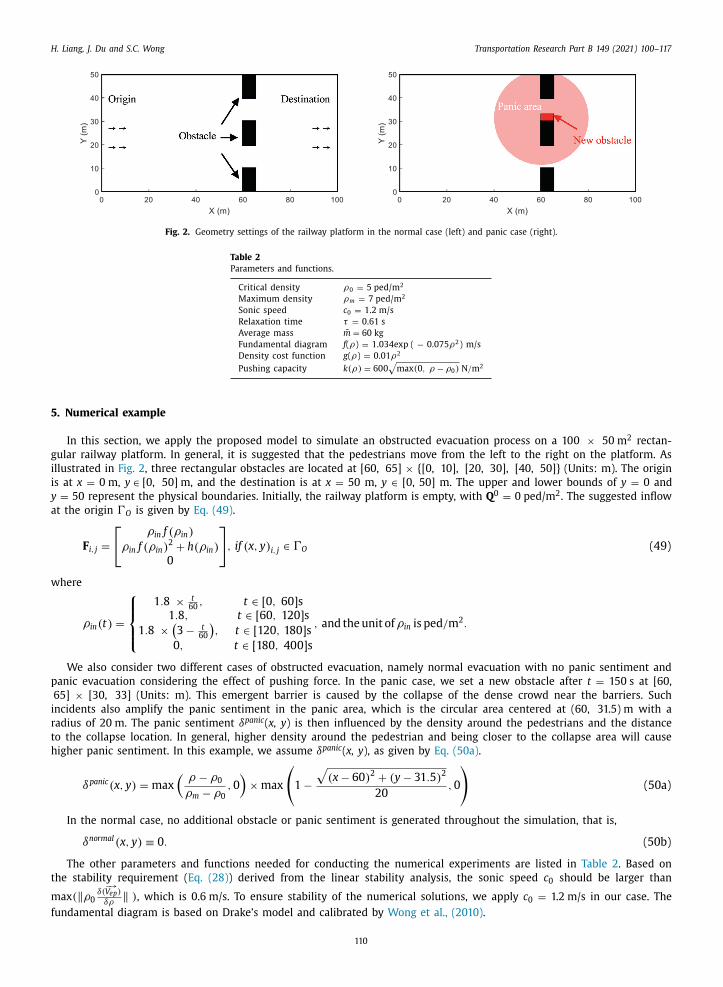
Fig. 2. Geometry settings of the railway platform in the normal case (left) and panic case (right).

Table 2

Parameters and functions.

Critical density ρ0 = 5 ped/m

2

Maximum density ρm = 7 ped/m

2

Sonic speed c 0 = 1.2 m/s

Relaxation time τ = 0.61 s

Average mass m = 60 kg

Fundamental diagram f ( ρ) = 1.034exp ( − 0.075 ρ2 ) m/s

Density cost function g ( ρ) = 0.01 ρ2

Pushing capacity k (ρ) = 600 √

max ( 0 , ρ − ρ0 ) N / m

2

5. Numerical example

In this section, we apply the proposed model to simulate an obstructed evacuation process on a 100 × 50 m

2 rectan-

gular railway platform. In general, it is suggested that the pedestrians move from the left to the right on the platform. As

illustrated in Fig. 2 , three rectangular obstacles are located at [60, 65] × {[0, 10], [20, 30], [40, 50]} (Units: m). The origin

is at x = 0 m, y ∈ [0, 50] m, and the destination is at x = 50 m, y ∈ [0, 50] m. The upper and lower bounds of y = 0 and

y = 50 represent the physical boundaries. Initially, the railway platform is empty, with Q

0 = 0 ped/m

2 . The suggested inflow

at the origin �O is given by Eq. (49) .

F i, j =

[

ρin f ( ρin )

ρin f ( ρin ) 2 + h ( ρin ) 0

]

, if ( x, y ) i, j ∈ �O (49)

where

ρin ( t ) =

⎧ ⎪ ⎨

⎪ ⎩

1 . 8 × t 60

, t ∈ [ 0 , 60 ] s 1 . 8 , t ∈ [ 60 , 120 ] s

1 . 8 ×(3 − t

60

), t ∈ [ 120 , 180 ] s

0 , t ∈ [ 180 , 400 ] s

, and the unit of ρin is ped / m

2 .

We also consider two different cases of obstructed evacuation, namely normal evacuation with no panic sentiment and

panic evacuation considering the effect of pushing force. In the panic case, we set a new obstacle after t = 150 s at [60,

65] × [30, 33] (Units: m). This emergent barrier is caused by the collapse of the dense crowd near the barriers. Such

incidents also amplify the panic sentiment in the panic area, which is the circular area centered at (60, 31.5) m with a

radius of 20 m. The panic sentiment δpanic ( x, y ) is then influenced by the density around the pedestrians and the distance

to the collapse location. In general, higher density around the pedestrian and being closer to the collapse area will cause

higher panic sentiment. In this example, we assume δpanic ( x, y ), as given by Eq. (50a) .

δpanic ( x, y ) = max

(ρ − ρ0

ρm

− ρ0

, 0

)× max

(

1 −√

( x − 60 ) 2 + ( y − 31 . 5 )

2

20

, 0

)

(50a)

In the normal case, no additional obstacle or panic sentiment is generated throughout the simulation, that is,

δnormal ( x, y ) ≡ 0 . (50b)

The other parameters and functions needed for conducting the numerical experiments are listed in Table 2 . Based on

the stability requirement ( Eq. (28) ) derived from the linear stability analysis, the sonic speed c 0 should be larger than

max ( ‖ ρ0 δ(

−→

V ep )

δρ‖ ) , which is 0.6 m/s. To ensure stability of the numerical solutions, we apply c 0 = 1.2 m/s in our case. The

fundamental diagram is based on Drake’s model and calibrated by Wong et al., (2010) .

110

H. Liang, J. Du and S.C. Wong Transportation Research Part B 149 (2021) 100–117

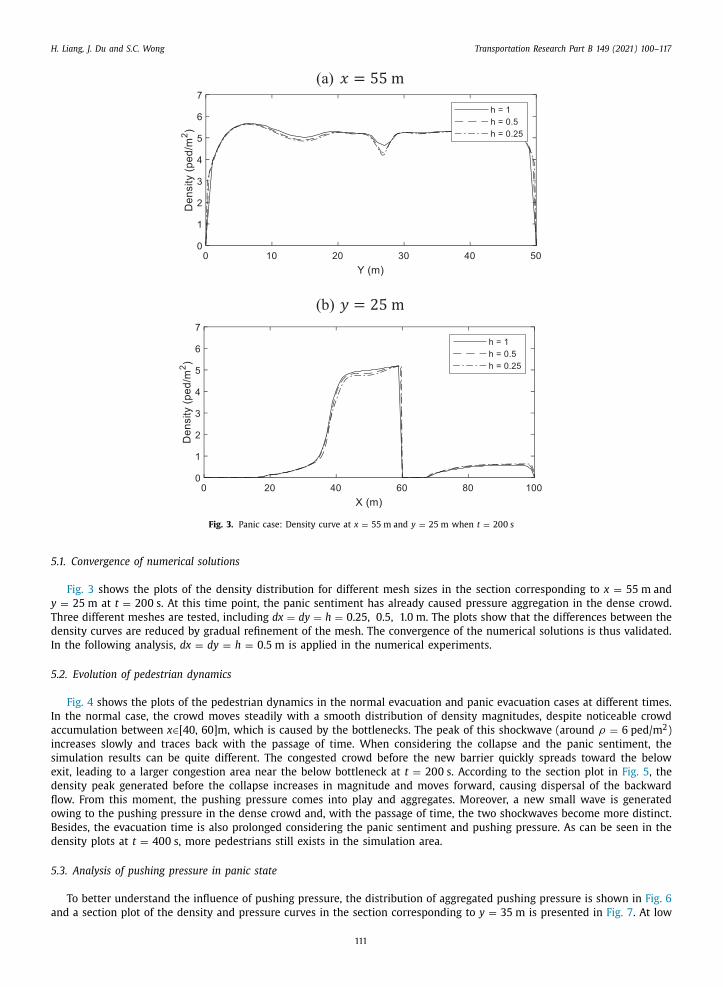
Fig. 3. Panic case: Density curve at x = 55 m and y = 25 m when t = 200 s

5.1. Convergence of numerical solutions

Fig. 3 shows the plots of the density distribution for different mesh sizes in the section corresponding to x = 55 m and

y = 25 m at t = 200 s. At this time point, the panic sentiment has already caused pressure aggregation in the dense crowd.

Three different meshes are tested, including dx = dy = h = 0.25, 0.5, 1.0 m. The plots show that the differences between the

density curves are reduced by gradual refinement of the mesh. The convergence of the numerical solutions is thus validated.

In the following analysis, dx = dy = h = 0.5 m is applied in the numerical experiments.

5.2. Evolution of pedestrian dynamics

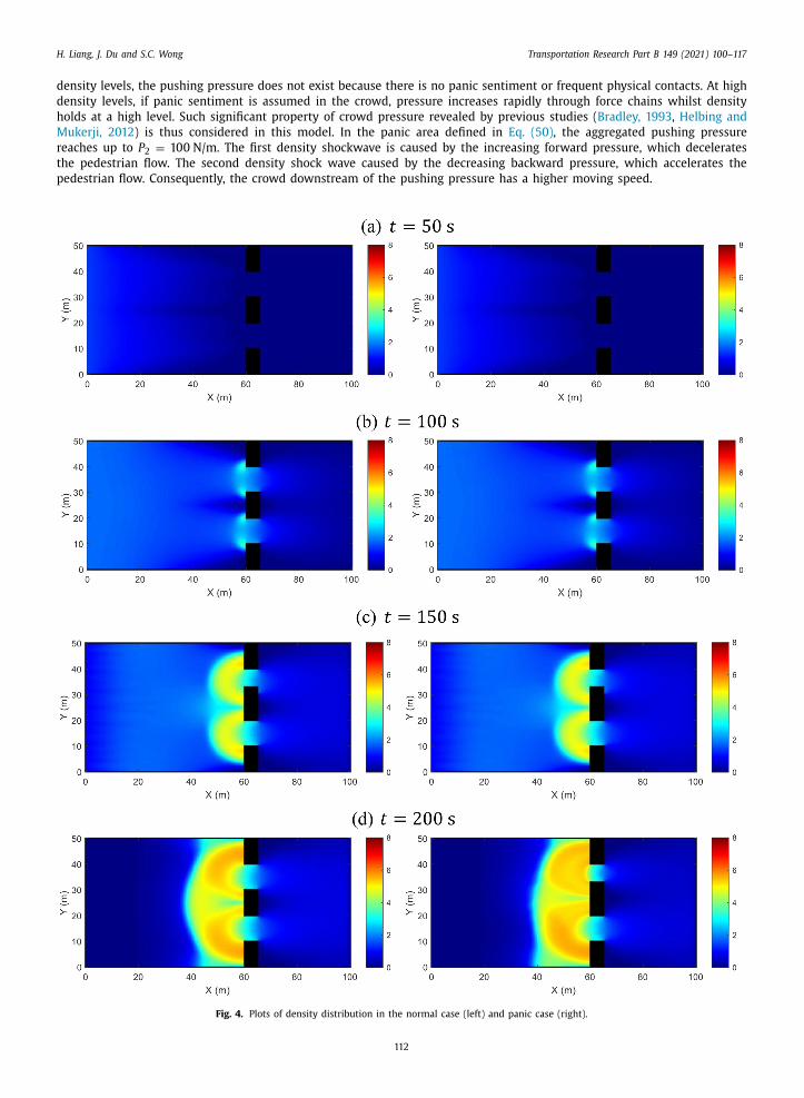
Fig. 4 shows the plots of the pedestrian dynamics in the normal evacuation and panic evacuation cases at different times.

In the normal case, the crowd moves steadily with a smooth distribution of density magnitudes, despite noticeable crowd

accumulation between x ∈ [40, 60]m, which is caused by the bottlenecks. The peak of this shockwave (around ρ = 6 ped/m

2 )

increases slowly and traces back with the passage of time. When considering the collapse and the panic sentiment, the

simulation results can be quite different. The congested crowd before the new barrier quickly spreads toward the below

exit, leading to a larger congestion area near the below bottleneck at t = 200 s. According to the section plot in Fig. 5 , the

density peak generated before the collapse increases in magnitude and moves forward, causing dispersal of the backward

flow. From this moment, the pushing pressure comes into play and aggregates. Moreover, a new small wave is generated

owing to the pushing pressure in the dense crowd and, with the passage of time, the two shockwaves become more distinct.

Besides, the evacuation time is also prolonged considering the panic sentiment and pushing pressure. As can be seen in the

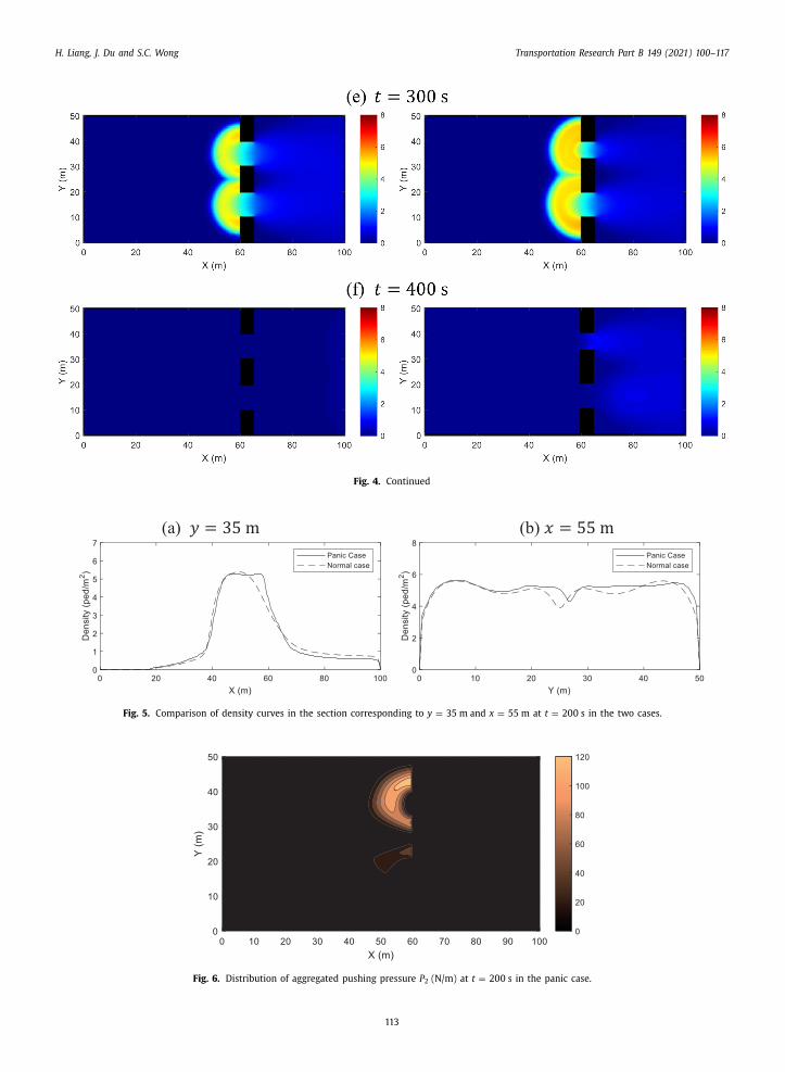
density plots at t = 400 s, more pedestrians still exists in the simulation area.

5.3. Analysis of pushing pressure in panic state

To better understand the influence of pushing pressure, the distribution of aggregated pushing pressure is shown in Fig. 6

and a section plot of the density and pressure curves in the section corresponding to y = 35 m is presented in Fig. 7 . At low

111

H. Liang, J. Du and S.C. Wong Transportation Research Part B 149 (2021) 100–117

density levels, the pushing pressure does not exist because there is no panic sentiment or frequent physical contacts. At high

density levels, if panic sentiment is assumed in the crowd, pressure increases rapidly through force chains whilst density

holds at a high level. Such significant property of crowd pressure revealed by previous studies ( Bradley, 1993 , Helbing and

Mukerji, 2012 ) is thus considered in this model. In the panic area defined in Eq. (50) , the aggregated pushing pressure

reaches up to P 2 = 100 N/m. The first density shockwave is caused by the increasing forward pressure, which decelerates

the pedestrian flow. The second density shock wave caused by the decreasing backward pressure, which accelerates the

pedestrian flow. Consequently, the crowd downstream of the pushing pressure has a higher moving speed.

Fig. 4. Plots of density distribution in the normal case (left) and panic case (right).

112

H. Liang, J. Du and S.C. Wong Transportation Research Part B 149 (2021) 100–117

Fig. 4. Continued

Fig. 5. Comparison of density curves in the section corresponding to y = 35 m and x = 55 m at t = 200 s in the two cases.

Fig. 6. Distribution of aggregated pushing pressure P 2 (N/m) at t = 200 s in the panic case.

113

H. Liang, J. Du and S.C. Wong Transportation Research Part B 149 (2021) 100–117

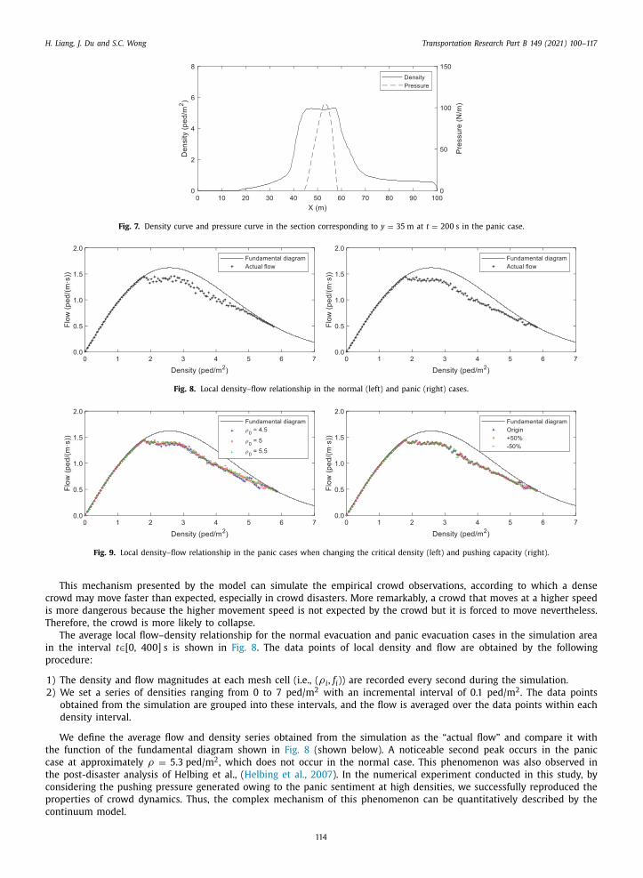
Fig. 7. Density curve and pressure curve in the section corresponding to y = 35 m at t = 200 s in the panic case.

Fig. 8. Local density–flow relationship in the normal (left) and panic (right) cases.

Fig. 9. Local density–flow relationship in the panic cases when changing the critical density (left) and pushing capacity (right).

This mechanism presented by the model can simulate the empirical crowd observations, according to which a dense

crowd may move faster than expected, especially in crowd disasters. More remarkably, a crowd that moves at a higher speed

is more dangerous because the higher movement speed is not expected by the crowd but it is forced to move nevertheless.

Therefore, the crowd is more likely to collapse.

The average local flow–density relationship for the normal evacuation and panic evacuation cases in the simulation area

in the interval t ∈ [0, 400] s is shown in Fig. 8 . The data points of local density and flow are obtained by the following

procedure:

1) The density and flow magnitudes at each mesh cell (i.e., ( ρ i , f i )) are recorded every second during the simulation.

2) We set a series of densities ranging from 0 to 7 ped/m

2 with an incremental interval of 0.1 ped/m

2 . The data points

obtained from the simulation are grouped into these intervals, and the flow is averaged over the data points within each

density interval.

We define the average flow and density series obtained from the simulation as the “actual flow” and compare it with

the function of the fundamental diagram shown in Fig. 8 (shown below). A noticeable second peak occurs in the panic

case at approximately ρ = 5.3 ped/m

2 , which does not occur in the normal case. This phenomenon was also observed in

the post-disaster analysis of Helbing et al., ( Helbing et al., 2007 ). In the numerical experiment conducted in this study, by

considering the pushing pressure generated owing to the panic sentiment at high densities, we successfully reproduced the

properties of crowd dynamics. Thus, the complex mechanism of this phenomenon can be quantitatively described by the

continuum model.

114

H. Liang, J. Du and S.C. Wong Transportation Research Part B 149 (2021) 100–117

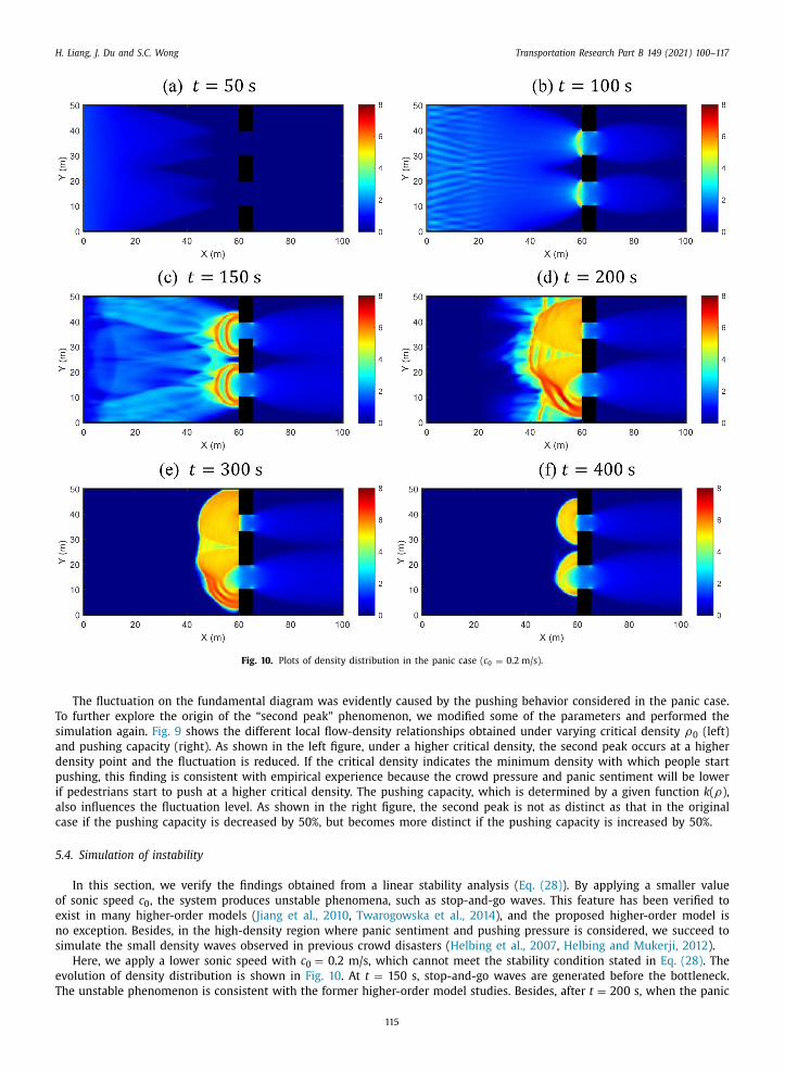
Fig. 10. Plots of density distribution in the panic case ( c 0 = 0.2 m/s).

The fluctuation on the fundamental diagram was evidently caused by the pushing behavior considered in the panic case.

To further explore the origin of the “second peak” phenomenon, we modified some of the parameters and performed the

simulation again. Fig. 9 shows the different local flow-density relationships obtained under varying critical density ρ0 (left)

and pushing capacity (right). As shown in the left figure, under a higher critical density, the second peak occurs at a higher

density point and the fluctuation is reduced. If the critical density indicates the minimum density with which people start

pushing, this finding is consistent with empirical experience because the crowd pressure and panic sentiment will be lower

if pedestrians start to push at a higher critical density. The pushing capacity, which is determined by a given function k ( ρ),

also influences the fluctuation level. As shown in the right figure, the second peak is not as distinct as that in the original

case if the pushing capacity is decreased by 50%, but becomes more distinct if the pushing capacity is increased by 50%.

5.4. Simulation of instability

In this section, we verify the findings obtained from a linear stability analysis ( Eq. (28) ). By applying a smaller value

of sonic speed c 0 , the system produces unstable phenomena, such as stop-and-go waves. This feature has been verified to

exist in many higher-order models ( Jiang et al., 2010 , Twarogowska et al., 2014 ), and the proposed higher-order model is

no exception. Besides, in the high-density region where panic sentiment and pushing pressure is considered, we succeed to

simulate the small density waves observed in previous crowd disasters ( Helbing et al., 2007 , Helbing and Mukerji, 2012 ).

Here, we apply a lower sonic speed with c 0 = 0.2 m/s, which cannot meet the stability condition stated in Eq. (28) . The

evolution of density distribution is shown in Fig. 10 . At t = 150 s, stop-and-go waves are generated before the bottleneck.

The unstable phenomenon is consistent with the former higher-order model studies. Besides, after t = 200 s, when the panic

115

H. Liang, J. Du and S.C. Wong Transportation Research Part B 149 (2021) 100–117

sentiment and pushing pressure are considered in the simulation, congested regions appear, as shown in Fig. 10 d . Small

waves continuously propagate in this high-density region, which indicates that the model is able to simulate turbulent-like

phenomena under certain conditions. These complex phenomena cannot be produced under stable conditions, as shown in

Fig. 4 , which indicates that the traffic instability must be simulated at a lower sonic speed.

6. Conclusion

In this paper, we proposed a new pedestrian dynamic model based on the 2D PW model. By relating the anticipation

term to crowd pressure, the new model was able to reveal the effects of the aggregated pushing force and the panic senti-

ment. Then, we performed linear stability analysis of the new dynamic model to determine its stability requirements. The

2D PDEs with relaxation were verified to remain stable under the given conditions. Based on the stability requirement, suit-

able parameters were set for the numerical experiments. Thus, the simulation of crowd movement was formulated as an

initial-value problem with a set of PDEs having appropriate boundary conditions.

To investigate the numerical properties of the proposed model, we develop a characteristic-wise WENO3 scheme to solve

the second-order system. Moreover, we solve the Eikonal-type equations using the third-order fast sweeping method, and

apply the third-order TVD Runge–Kutta time discretization method to perform time integration. The numerical results can be

obtained in any simulation case. In the numerical example, we consider both normal evacuation and panic evacuation cases.

A comparison of the numerical results obtained in different cases reveals the macroscopic characteristics of the proposed

model. A significant property of crowd pressure is revealed by the simulation results: at high density, if panic sentiment

is assumed in the crowd, the pressure increases rapidly through force chains while the density is maintained at a high

level. Thus, the crowd pressure estimated in the simulation can be used as a risk-level indicator for crowd management

and control. Besides, the local flow-density relationship derived using the proposed model produces the second peak in the

high-density regions, which is consistent with previous empirical studies. Furthermore, complex phenomena of stop-and-go

waves is reproduced by applying suitable parameters obtained from linear stability analysis.

Further studies of this pedestrian dynamics model will focus on the calibration of the parameters through field exper-

iments, exploration of internal friction and application to multi-direction pedestrian flow. The key problem in our current

model, which has not been solved by previous studies, is to calibrate the pushing pressure and compression pressure. Sev-

eral experiment-based studies have introduced wearable pressure sensors. Wang and Weng (2018) applied a high-tech tactile

vest to measure the collision force along a queue, and Song et al., (2019) established the relationship between the maxi-

mum crowding force and density based on the tactile data recorded in a metro carriage. Inspired by these studies, we will

conduct a field experiment on a small group of participants to calibrate the key parameters used in the model, includ-

ing the compression pressure and pushing pressure. We will adopt wearable sensor products and stationary force sensors

to establish the relationships between the pressure magnitudes and density, which are assumed in the current paper. The

wearable sensor products will be used to measure the compression pressure while the stationary force sensors will measure

the pushing capacity of a single group of people. Thus, the relationships assumed in the current paper will be calibrated. As

it would be unethical to simulate panic during an experiment, the validation of pressure magnitudes is difficult. Therefore,

our future work will focus on developing crowd models of multidirectional cases, simulating real crowd disasters (e.g. the

Love Parade disaster) and identifying the potentially dangerous areas and periods. By comparing the simulation results with

the real disasters, we will validate our model to the greatest extent possible and determine its practical value.

CRediT author statement

Liang Haoyang: Conceptualization, Modeling, Simulation, Writing- Original draft preparation.

Du Jie : Methodology, Analytical review.

Wong S. C. : Supervision, Conceptualization, Writing - Review & Editing.

Acknowledgments

The work described in this paper was supported by grants from the Research Grants Council of the Hong Kong Special

Administrative Region, China (Project Nos. 17201318, 17204919), and Guangdong - Hong Kong - Macau Joint Laboratory

Program of the 2020 Guangdong New Innovative Strategic Research Fund, Guangdong Science and Technology Department

(Project No.: 2020B1212030 0 09). The first author was supported by a Postgraduate Scholarship from the University of Hong

Kong, the second author by National Natural Science Foundation of China (Grant No. 11801302) and Tsinghua University

Initiative Scientific Research Program, and the third author by the Francis S Y Bong Professorship in Engineering from the

University of Hong Kong.

References

Aw, A .A .T.M. , Rascle, M , 20 0 0. Resurrection of “second order” models of traffic flow. SIAM Journal on Applied Mathematics 60, 916–938 .

Bauer, D. , Seer, S. , Brändle, N. , 2007. Macroscopic pedestrian flow simulation for designing crowd control measures in public transport after special events.In: Proceedings of the 2007 Summer Computer Simulation Conference, pp. 1035–1042 .

116

H. Liang, J. Du and S.C. Wong Transportation Research Part B 149 (2021) 100–117

Bradley, G.E. , 1993. A proposed mathematical model for computer prediction of crowd movements and their associated risks. . Engineering for Crowd Safety303–311 .

Cao, K. , Chen, Y. , Stuart, D. , Yue, D. , 2015. Cyber-physical modeling and control of crowd of pedestrians: a review and new framework. IEEE/CAA Journal ofAutomatica Sinica 2, 334–344 .

Dickie, J.F. , Wanless, G.K. , 1993. Spectator terrace barriers. Structural Engineer 71, 216 . Fruin, J. , 1993. The causes and prevention of crowd disasters. Engineering for Crowd Safety 1, 99–108 .

Helbing, D. , Farkas, I.J. , Vicsek, T. , 20 0 0. Simulating dynamical features of escape panic. Nature 407, 4 87–4 90 .

Helbing, D. , Johansson, A. , 2009. Pedestrian, Crowd and Evacuation Dynamics. Springer . Helbing, D. , Johansson, A. , Al-Abideen, H.Z. , 2007. Dynamics of crowd disasters: An empirical study. Physical Review E 75, 046109 .

Helbing, D. , Mukerji, P. , 2012. Crowd disasters as systemic failures: analysis of the Love Parade disaster. EPJ Data Science 1 (7), 1–40 . Hopkins, I.H.G. , Pountney, S.J. , Hayes, P. , Sheppard, M.A , 1993. Crowd pressure monitoring. Engineering for Crowd Safety 389–398 .

Huang, L. , Wong, S.C. , Zhang, M. , Shu, C. , Lam, W. , 2009. Revisiting Hughes’ dynamic continuum model for pedestrian flow and the development of anefficient solution algorithm. Transportation Research Part B 43, 127–141 .

Hughes, R.L. , 2002. A continuum theory for the flow of pedestrians. Transportation Research Part B 36, 507–535 . Jiang, Y.Q. , Zhang, P. , Wong, S.C. , Liu, R.X. , 2010. A higher-order macroscopic model for pedestrian flows. Physica A: Statistical Mechanics and its Applications

389, 4623–4635 .

Jiang, Y.Q. , Zhang, W. , Zhou, S.G. , 2016. Comparison study of the reactive and predictive dynamic models for pedestrian flow. Physica A: Statistical Mechanicsand its Applications 441, 51–61 .

Johansson, A. , Helbing, D. , Al-Abideen, H.Z. , Al-Bosta, S. , 2008. From crowd dynamics to crowd safety: a video-based analysis. Advances in Complex Systems11, 497–527 .

Karamouzas, I. , Skinner, B. , Guy, S.J. , 2014. Universal power law governing pedestrian interactions. Physical Review Letters 113, 238701 . Keating, J.P. , 1982. The myth of panic. Fire Journal 76, 57–61 .

Langston, P.A. , Masling, R. , Asmar, B.N. , 2006. Crowd dynamics discrete element multi-circle model. Safety Science 44, 395–417 .

Lin, P. , Ma, J. , Si, Y. , Wu, F. , Wang, G. , Wang, J. , 2017. A numerical study of contact force in competitive evacuation. Chinese Physics B 26, 104501 . Lu, C. , 2007. Analysis of compressed force in crowds. Journal of Transportation Systems Engineering and Information Technology 7, 98–102 .

Moussaïd, M. , Helbing, D. , Theraulaz, G. , 2011. How simple rules determine pedestrian behavior and crowd disasters. Proceedings of the National Academyof Sciences 108, 6 884–6 888 .

Payne, H.J. , 1971. Models of freeway traffic and control. Mathematical Models of Public Systems 1, 51–61 . Ren, Y. , Zhang, H. , 2003. A characteristic-wise hybrid compact-WENO scheme for solving hyperbolic conservation laws. Journal of Computational Physics

192, 365–386 .

Shu, C.W. , Osher, S. , 1988. Efficient implementation of essentially non-oscillatory shock capturing schemes. Journal of Computational Physics 77, 439–471 . Smith, R.A. , Lim, L.B. , 1995. Experiments to investigate the level of ‘comfortable’ loads for people against crush barriers. Safety Science 18, 329–335 .

Song, J. , Chen, F. , Zhu, Y. , Zhang, N. , Liu, W. , Du, K. , 2019. Experiment Calibrated Simulation Modeling of Crowding Forces in High Density Crowd. IEEEAccess 7, 100162–100173 .

Twarogowska, M. , Goatin, P. , Duvigneau, R. , 2014. Macroscopic modeling and simulations of room evacuation. Applied Mathematical Modelling 38,5781–5795 .

Wang, C. , Weng, W. , 2018. Study on the collision dynamics and the transmission pattern between pedestrians along the queue. Journal of Statistical Me-

chanics: Theory and Experiment 1–27 2018 . Wong, S.C. , Leung, W.L. , Chan, S.H. , Lam, W.H.K. , Yung, N.H.C. , Liu, C.Y. , Zhang, P , 2010. Bidirectional pedestrian stream model with oblique intersecting

angle. Journal of transportation Engineering 136, 234–242 . Zhan, B. , Monekosso, D.N. , Remagnino, P. , Velastin, S.A. , Xu, L.Q. , 2008. Crowd analysis: a survey. Machine Vision and Applications 19, 345–357 .

Zhang, X. , Weng, W. , Yuan, H. , Chen, J. , 2013. Empirical study of a unidirectional dense crowd during a real mass event. Physica A: Statistical Mechanicsand its Applications 392, 2781–2791 .

Zhang, Y.T. , Zhao, H.K. , Qian, J.L. , 2006. High order fast sweeping methods for static Hamilton–Jacobi equations. Journal of Scientific Computing 29, 25–56 .

Zhao, R. , Hu, Q. , Liu, Q. , Li, C. , Dong, D. , Ma, Y. , 2019. Panic propagation dynamics of high-density crowd based on information entropy and Aw-Rasclemodel. IEEE Transactions on Intelligent Transportation Systems 1–10 .

117