testing humidity sensors
TRANSCRIPT

Q&A: Engineering “Moonshot” Projects Vehicle Monitoring System Design | Testing Humidity Sensors | DIY Particulate Matter Monitor Project
| Network-Ready Music Controller Phase Change Material-Based Cooling | Understanding the Physics of Shielding | Pulsed Motor Drive
| Programmable Logic Controller Export File The Future of Intelligent Robots
MEASUREMENT & SENSORS MAY 2015 ISSUE 298CIRCUIT CELLAR | ISSUE 298 | M
AY 2015circuitcellar.com
circuitcellar.com
Innovative Sensor-Based Technologies
Multiple new options available for our IP67 ultrasonic sensors

PC OSCILLOSCOPES
Low cost
MSO
Eight channels
2 GS memory
Flexible resolution
20 GHzsampling
www.picotech.com/pco5401-800-591-2796
• 10 MHz to 200 MHz bandwidth• 100 MS to 1 GS/s sampling• 8 bit resolution (12 bit enhanced)• 8 to 48 kS buffer memory• USB powered• Prices from $131
• 2 or 4 analog channels + 16 digital• 50 to 200 MHz bandwidth• 8 bit resolution (12 bit enhanced)• 64 to 512 MS buffer memory• USB or AC adaptor powered• Prices from $824
• 20 MHz bandwidth• 80 MS/s sampling• 12 bit resolution (16 bit enhanced) • 256 MS buffer memory • USB powered• Just $2302
• 8, 12, 14, 15 & 16 bits all in one device• 60 to 200 MHz bandwidth • 250 MS/s to 1 GS/s sampling• 8 to 512 MS buffer memory • USB or AC adaptor powered• Prices from $1153
• 250 MHz to 1 GHz bandwidth• 5 GS/s sampling • 8 bit resolution (12 bit enhanced)• 256 MS to 2 GS buffer memory • AC adaptor powered• Prices from $3292
• DC to 20 GHz bandwidth• 17.5 ps rise time• 16 bit, 60 dB dynamic range• AC adaptor powered• Sig. gen, CDR, diff. TDR/TDT• Prices from $14,995
Full software included as standard with serial bus decoding and analysis (CAN, LIN, RS232, I2C, I2S, SPI, FlexRay), segmented memory, mask testing, spectrum analysis, and software development kit (SDK) all as standard, with free software updates. Five years warranty real time oscilloscopes, 2 years warranty sampling oscilloscopes.
20 GHzg
tion
CIRCUIT CELLAR • MAY 2015 #2982
Issue 298 May 2015 | ISSN 1528-0608
CIRCUIT CELLAR® (ISSN 1528-0608) is published monthly by:
Circuit Cellar, Inc.111 Founders Plaza, Suite 904
East Hartford, CT 06108
Periodical rates paid at East Hartford, CT, and additional offices. One-year (12 issues) subscription rate US and possessions
$50, Canada $65, Foreign/ ROW $75. All subscription orders payable in US funds only via Visa, MasterCard, international
postal money order, or check drawn on US bank.
SUBSCRIPTIONS
Circuit Cellar, P.O. Box 462256, Escondido, CA 92046
E-mail: [email protected]
Phone: 800.269.6301
Internet: circuitcellar.com
Address Changes/Problems: [email protected]
Postmaster: Send address changes to Circuit Cellar, P.O. Box 462256, Escondido, CA 92046
ADVERTISING
Strategic Media Marketing, Inc.2 Main Street, Gloucester, MA 01930 USA
Phone: 978.281.7708
Fax: 978.281.7706
E-mail: [email protected] rates and terms available on request.
New Products:New Products, Circuit Cellar, 111 Founders Plaza, Suite 904
East Hartford, CT 06108, E-mail: [email protected]
HEAD OFFICE
Circuit Cellar, Inc. 111 Founders Plaza, Suite 904East Hartford, CT 06108
Phone: 860.289.0800
COVER PHOTOGRAPHY
Chris Rakoczy, www.rakoczyphoto.com
COPYRIGHT NOTICE
Entire contents copyright © 2015 by Circuit Cellar, Inc. All rights reserved. Circuit Cellar is a registered trademark of Circuit Cellar, Inc. Reproduction of this publication in whole or in part without written consent from Circuit Cellar, Inc. is
prohibited.
DISCLAIMER
Circuit Cellar® makes no warranties and assumes no responsibility or liability of any kind for errors in these programs or schematics or for the consequences of any
such errors. Furthermore, because of possible variation in the quality and condition of materials and workmanship of reader-assembled projects, Circuit Cellar® disclaims any responsibility for the safe and proper function of reader-
assembled projects based upon or from plans, descriptions, or information published by Circuit Cellar®.
The information provided by Circuit Cellar® is for educational purposes. Circuit Cellar® makes no claims or warrants that readers have a right to build things based upon these ideas under patent or other relevant intellectual property law in
their jurisdiction, or that readers have a right to construct or operate any of the devices described herein under the relevant
patent or other intellectual property law of the reader’s jurisdiction. The reader assumes any risk of infringement
liability for constructing or operating such devices.
© Circuit Cellar 2015 Printed in the United States
THE TEAM
EDITOR-IN-CHIEFC. J. Abate
ART DIRECTORKC Prescott
ADVERTISING COORDINATORKim Hopkins
PRESIDENTHugo Van haecke
COLUMNISTS
Jeff Bachiochi (From the Bench), Ayse K. Coskun
(Green Computing), Bob Japenga (Embedded in Thin Slices), Robert Lacoste (The Darker Side), Ed Nisley (Above the Ground Plance), George Novacek (The Consummate Engineer), and Colin O’Flynn (Programmable Logic in Practice)
FOUNDERSteve Ciarcia
PROJECT EDITORSChris Coulston, Ken Davidson, and David Tweed
OFFICE ASSISTANTDebbie Lavoie
TOPICS IN MEASUREMENT & SENSOR TECHThis issue comprises several articles about innovative microcontroller-based
measurement and sensor systems. Whether your goal is to develop the next blockbuster IoT product or simply build a handy home control module, this issue is will provide you with the tips, tricks, and inspiration to get started.
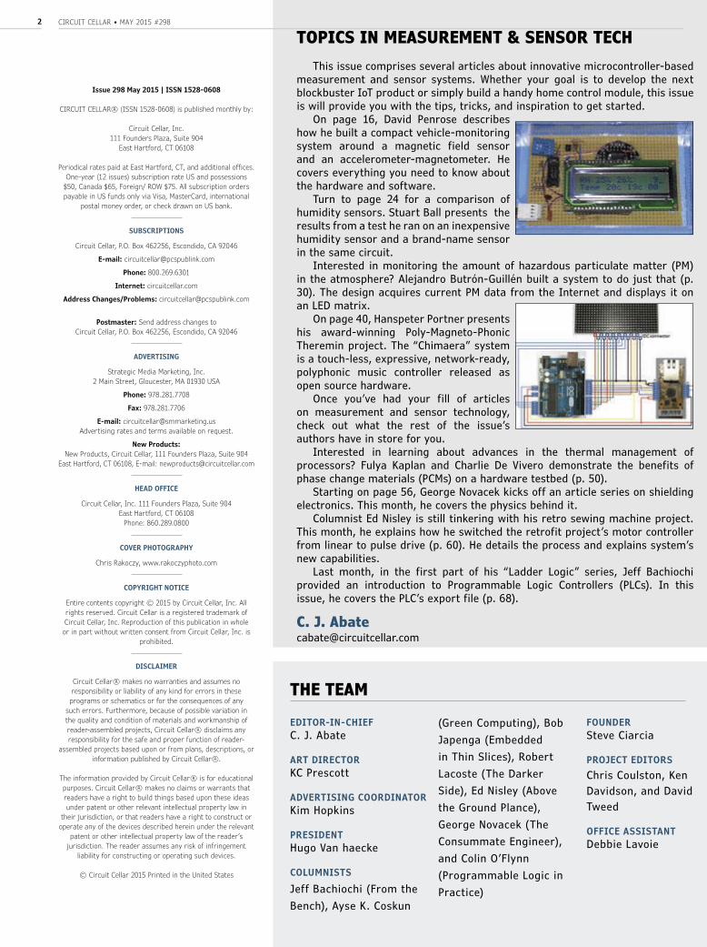
On page 16, David Penrose describes how he built a compact vehicle-monitoring system around a magnetic field sensor and an accelerometer-magnetometer. He covers everything you need to know about the hardware and software.
Turn to page 24 for a comparison of humidity sensors. Stuart Ball presents the results from a test he ran on an inexpensive humidity sensor and a brand-name sensor in the same circuit.
Interested in monitoring the amount of hazardous particulate matter (PM) in the atmosphere? Alejandro Butrón-Guillén built a system to do just that (p. 30). The design acquires current PM data from the Internet and displays it on an LED matrix.
On page 40, Hanspeter Portner presents his award-winning Poly-Magneto-Phonic Theremin project. The “Chimaera” system is a touch-less, expressive, network-ready, polyphonic music controller released as open source hardware.
Once you’ve had your fill of articles on measurement and sensor technology, check out what the rest of the issue’s authors have in store for you.
Interested in learning about advances in the thermal management of processors? Fulya Kaplan and Charlie De Vivero demonstrate the benefits of phase change materials (PCMs) on a hardware testbed (p. 50).
Starting on page 56, George Novacek kicks off an article series on shielding electronics. This month, he covers the physics behind it.
Columnist Ed Nisley is still tinkering with his retro sewing machine project. This month, he explains how he switched the retrofit project’s motor controller from linear to pulse drive (p. 60). He details the process and explains system’s new capabilities.
Last month, in the first part of his “Ladder Logic” series, Jeff Bachiochi provided an introduction to Programmable Logic Controllers (PLCs). In this issue, he covers the PLC’s export file (p. 68).
C. J. [email protected]

circuitcellar.com 3
OUR NETWORK
SUPPORTING COMPANIES
NOT A SUPPORTING COMPANY YET?
Contact Peter Wostrel ([email protected], Phone 978.281.7708, Fax 978.281.7706) to reserve your own space for the next edition of our members’ magazine.
Accutrace 7
All Electronics Corp. 79
AP Circuits 71
Custom Computer Services 79
EMAC, Inc. 63
ESC 2015 - Boston 43
ESC 2015 - Silicon Valley 65
Front Panel 71
HuMANDATA, Ltd. 63
IAR Systems 19
Imagineering, Inc. C4
Ironwood Electronics 79
Jeffery Kerr, LLC 79
Lemos International 21
MaxBotix, Inc. C2, 79
Measurement Computing Corp. 55
microEngineering Labs, Inc. 79
Mouser Electronics 23
MyRO Electronic Control Devices, Inc. 79
NetBurner, Inc. 11, 29
Newhaven Display International 39
Pico Technology, Ltd. 1
Saelig Co., Inc. 21
Sensors Expo & Conference 49
Technologic Systems 35, 59
Vintage Computer Festival 79
FOUNDERSteve Ciarcia
PROJECT EDITORSChris Coulston, Ken Davidson, and David Tweed
OFFICE ASSISTANTDebbie Lavoie

CIRCUIT CELLAR • MAY 2015 #2984
CONTENTS MAY 2015 • ISSUE 298
MEASUREMENT & SENSORS
CC COMMUNITY06 : QUESTIONS & ANSWERSEngineering "Moonshot" ProjectsAn Interview with Andrew Meyer The LeafLabs co-founder talks about innovative designs and the future of electrical engineering
INDUSTRY & ENTERPRISE12 : PRODUCT NEWS
15 : CLIENT PROFILELS Research (Cedarburg, WI)
FEATURES16 : A Different SenseVehicle Monitoring with a Magnetic Field Sensor SystemBy David PenroseA vehicle sensor system built around a magnetic field sensor and an accelerometer-magnetometer 24 : Comparing Humidity SensorsBy Stuart BallTesting the efficacy of an inexpensive humidity sensor against a brand-name sensor in the same circuit
30 : Atmospheric Particulate Matter MonitorBy J. Alejandro Butrón-Guillén DIY atmosphere monitor that retrieves particulate matter data from the ‘Net and displays it on an LED
BUILD VEHICLE SENSOR SYSTEM
SBC WITH COPPER BOX HOLDING PHASE CHANGE MATERIALBEHIND THE SCENES AT LEAFLABS
circuitcellar.com 5
CONTENTS
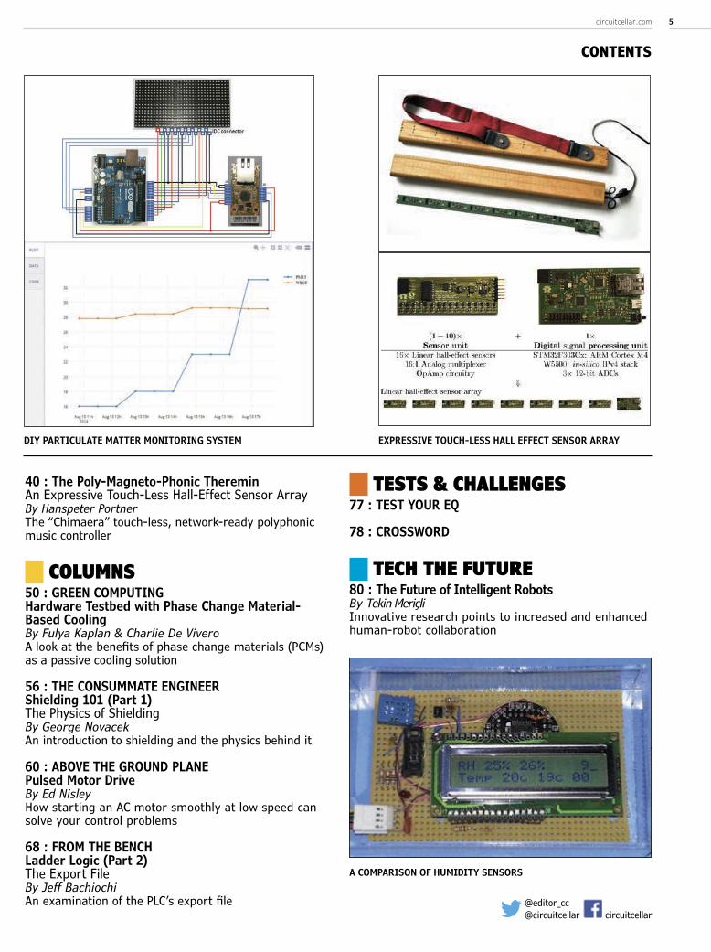
40 : The Poly-Magneto-Phonic ThereminAn Expressive Touch-Less Hall-Effect Sensor ArrayBy Hanspeter PortnerThe “Chimaera” touch-less, network-ready polyphonic music controller
COLUMNS50 : GREEN COMPUTINGHardware Testbed with Phase Change Material-Based CoolingBy Fulya Kaplan & Charlie De ViveroA look at the benefits of phase change materials (PCMs) as a passive cooling solution
56 : THE CONSUMMATE ENGINEERShielding 101 (Part 1)The Physics of ShieldingBy George NovacekAn introduction to shielding and the physics behind it
60 : ABOVE THE GROUND PLANEPulsed Motor DriveBy Ed NisleyHow starting an AC motor smoothly at low speed can solve your control problems 68 : FROM THE BENCHLadder Logic (Part 2)The Export FileBy Jeff BachiochiAn examination of the PLC’s export file
TESTS & CHALLENGES77 : TEST YOUR EQ
78 : CROSSWORD
TECH THE FUTURE80 : The Future of Intelligent RobotsBy Tekin MeriçliInnovative research points to increased and enhanced human-robot collaboration
EXPRESSIVE TOUCH-LESS HALL EFFECT SENSOR ARRAY
@editor_cc@circuitcellar circuitcellar
DIY PARTICULATE MATTER MONITORING SYSTEM
A COMPARISON OF HUMIDITY SENSORS
CIRCUIT CELLAR • MAY 2015 #2986CO
MM
UNIT
Y
QUESTIONS & ANSWERS
CIRCUIT CELLAR: How did you become interested in electronics? Did you start at a young age?
ANDREW: Yes, actually, but I am not sure I really got anywhere fooling around as a kid. I had a deep love of remote control cars and airplanes in middle school. I was totally obsessed with figuring out how to build my own control radio. This was right before the rise of Google, and I scoured the net for info on circuits. In the end, I achieved a reasonable grasp on really simple RC type circuits but completely failed in figuring out the radio. Later in high school I took some courses at the local community college and built an AM radio and got into the math for the first time - j and omega and all that.
CIRCUIT CELLAR: What led you MIT and your course of study there? For instance, why didn’t you pursue chemistry or physics?
ANDREW: MIT was an early obsession. Rod Brook’s lab was working on COG—this humanoid robot—that just blew me away. I started sending the graduate students emails. A couple wrote back and I fell in love with the idea of joining them one day. Why not physics? Easy. At MIT I quickly realized I was not in the same league, in terms of mathematical ability, as the kids that were going to excel in physics. Besides, my first love was AI and robotics.
CIRCUIT CELLAR: Tell us about your involvement in MIT’s Robot Locomotion Group. What were some of th projects you worked on?
ANDREW: One of MIT’s best features is undergraduate research. I had the privilege of working under Russ Tedrake in his lab. He was
an amazing mentor—as were his students—and everyone treated me like a graduate student even though I wasn’t. I often regret I did not put more hours in his lab, but I got one hell of an education just hanging around. I was paired up with Rick Cory, a PhD student focused on control systems for aircraft that could perform various acrobatics. This is a hard problem because once you go into a stall, the dynamics get crazy and you lose a ton of control authority. Flight is a particularly fun problem because aerodynamics provide plenty of dynamical regimes that are chaotic. We used reinforcement learning to develop controllers that could handle some of this chaos. The work culminated in an autonomous glider that could “perch”—basically, a highly controlled vertical stall. On a different robot, a flapping winged ornithopter, we had this PC104 computer running MATLAB as the controller. It probably weighed about 2 lbs, which forced us to build a huge wingspan—almost 6 . We dreamed about adding some machine vision to the platform as well. Having just built a vision-based robot for MIT’s MASLAB competition using an FPGA paired with an Arduino—the PC104 solution started to look pretty stupid to me. That was what really got me interested embedded work. FPGAs and microcontrollers gave you an insane amount of computing power at comparatively minuscule power and weight footprints. And so died the PC104 standard.
CIRCUIT CELLAR: Tell us about your internship at Analog Devices. Can you tell us about what you worked on?
ANDREW: I got the job at Analog after some folks there saw our MASLAB robot I mentioned earlier. I worked in the MEMS group that
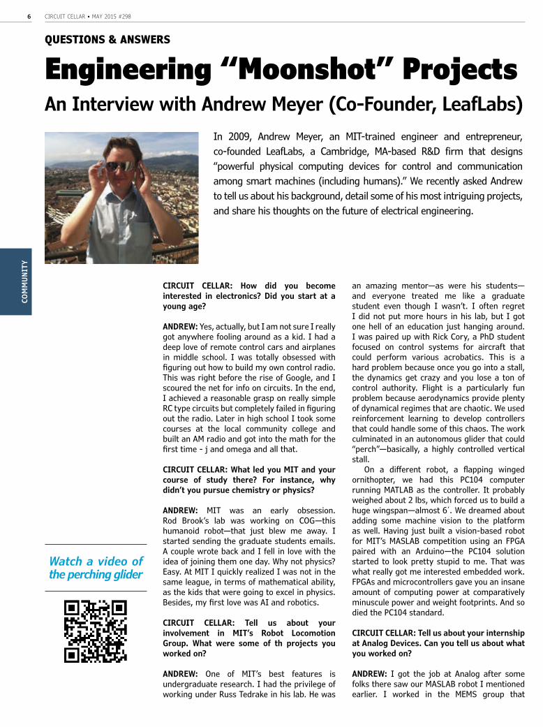
Engineering “Moonshot” Projects An Interview with Andrew Meyer (Co-Founder, LeafLabs)
In 2009, Andrew Meyer, an MIT-trained engineer and entrepreneur, co-founded LeafLabs, a Cambridge, MA-based R&D firm that designs “powerful physical computing devices for control and communication among smart machines (including humans).” We recently asked Andrew to tell us about his background, detail some of his most intriguing projects, and share his thoughts on the future of electrical engineering.
Watch a video of the perching glider

THERE ARE NO GAMES INVOLVED IN OUR PRICING
Take the Accutrace Challenge and see WHY OUR PRICING CANNOT BE BEATEN
www.PCB4u.com [email protected]
CIRCUIT CELLAR • MAY 2015 #2988CO
MM
UNIT
Y
QUESTIONS & ANSWERS
was responsible for the XL345. This was the accelerometer used in the Nintendo Wii, so we all felt a bit like rockstars. iPhone had just come out, and so everyone was dreaming about using these types of devices in smartphones. Analog was where I really cut my teeth on the Cortex M3, which we used in our test hardware for the part.
CIRCUIT CELLAR: What was the most important thing you learned during your internship at Analog Devices?
ANDREW: Certainly the most surprising thing I learned was that in the land of digital logic and RTL, verification engineers outnumber design engineers by about 6 to 1. When going to fab costs at six or seven figures, you need to be sure that things are going to work. Despite the enormous amount of simulation, you still never get it on the first try though. I won’t mention how many tries it took on that part.
CIRCUIT CELLAR: What is Leaflabs? How did it start? Who comprises your team today?
ANDREW: LeafLabs is an R&D firm specializing in embedded and distributed systems. Projects start as solving specific problems for a client, but the idea is to turn those relationships into product opportunities. To me, that’s what separates R&D from consulting. I started LeafLabs with a handful of friends in 2009. It was an all MIT cast of engineers, and it took four or five years before I understood how much we were holding ourselves back by not embracing some marketing and sales talent. The original concept was to try and design ICs that were optimized for running certain machine learning algorithms at low power. The idea was that smartphones might want to do speech to text some day without sending the audio off to the cloud. This was way too ambitious for a
group of 22 year olds with no money. Our second overly ambitious idea was to try and solve the “FPGA problem.” I’m still really passionate about this, but it too was too much for four kids in a basement to take a big bite off. The problem is that FPGAs vendors like Xilinx and Altera have loads of expertise in silicon, but great software is just not in their DNA. Imagine if x86 never published their instruction set. What if Intel insisted on owning not just the processors, but the languages, compilers, libraries, IDEs, debuggers, operating systems, and the rest of it? Would we ever have gotten to Linux? What about Python? FPGAs have enormous potential to surpass even the GPU as a completely standard technology in computer systems. There should some gate fabric in my phone. The development tools just suck, suck, suck. If any FPGA executives are reading this: Please open up your bitstream formats, the FSF and the rest of the community will get the ball rolling on an open toolchain that will far exceed what you guys are doing internally. You will change the world.
CIRCUIT CELLAR: How did the Maple microcontroller board come about?
ANDREW: Arduino was really starting to come up at the time. I had just left Analog, where we had been using the 32-bit Cortex M3. We started asking “Chips like the STM32 are clearly the way of the future, why on earth is Arduino using a chip from the ‘90s?” Perry, another LeafLabs founder, was really passionate about this. ARM is taking over the world, the community deserves a product that is as easy to use as Arduino, but built on top of modern technology.
CIRCUIT CELLAR: Can you give a general overview of your involvement with Project Ara?
ANDREW: We got into Ara at the beginning as subcontractors to the company that was leading
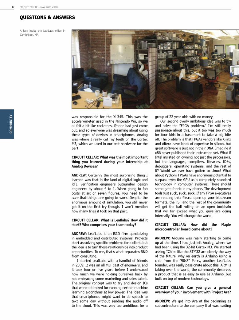
A look inside the LeafLabs office in Cambridge, MA

circuitcellar.com 9COM
MUNITY
QUESTIONS & ANSWERS
a lot of the engineering, NK Labs. Since then our role has expanded quite a bit, but we are still focused on software and firmware development. Everyone understood that Ara was going to require a lot of firmware and FPGA work, and so we were a natural choice to get involved. One of the first Ara prototypes actually used the Maple software library, libmaple, and had eight FPGAs in it! For your readers that are interested in Ara, please to check out projectara.com and https://github.com/projectara/greybus/.
LeafLabs is focused on firmware development. What’s really exciting to me about the project is the technology under the hood. Basically, what we have done is built a network on a PCB. The first big problem with embedded linux devices is that they are completely centered around the SoC. Change the SoC and you are in for ton of software development, for instance, to bring your display driver back to life. Similarly, changes to the design, such as incorporating a faster Wi-Fi chip, might force you to change the SoC. This severe coupling between everything keeps designers from iterating. You have this attitude of “OK, no one touch this design for the next 5 years, we finally got it working.” If we have learned anything from SaaS and App companies it’s that quickly iterating and continuous deployment are key to great products. If your platform inhibits iteration, you have a big problem. The other problem with embedded systems is that there are so many protocols! SDIO, USB,
DSI, I2C, SPI, CSI, blah blah blah. Do we really need so many!? Think how much mileage we get out of TCP/IP. The protocol explosion just adds impedance to the entire design process, and forces engineers to be worrying about bits toggling on traces rather than customer facing features. The technology being developed for Ara, called Greybus, solves both these problems. The centerpiece of our phone is a switch, and the display, Wi-Fi, audio, baseband, etc all
hang off the switch as network devices. Even the processor is just another module hanging off this network. All modules speak the same “good enough” protocol called UniPro (Unified Protocol). The possibilities here are absolutely tantalizing. To learn more about Greybus, see here: https://github.com/projectara/greybus/.
CIRCUIT CELLAR: Can you define “minimalist data acquisition” for our readers? What is it and why does it interest you?
ANDREW: More and more fields, but particularly in neuroscience, are having to deal with outrageously huge real-time data sets. There are 100 billion neurons in the human brain. If we want to listen to just 1,000 of them, we are already talking about ~1 Gbps. Ed Boyden, a professor at MIT, asked us if we could build some hardware to help handle the torrent. Could we scale to 1 Tbps? Could we build something that researchers on a budget
“If any FPGA executives are reading this: Please open up your bitstream formats, the FSF and the rest of the community will get the ball rolling on an open toolchain that will far exceed what you guys are doing internally. You will change the world.”
CIRCUIT CELLAR • MAY 2015 #29810CO
MM
UNIT
Y
QUESTIONS & ANSWERS
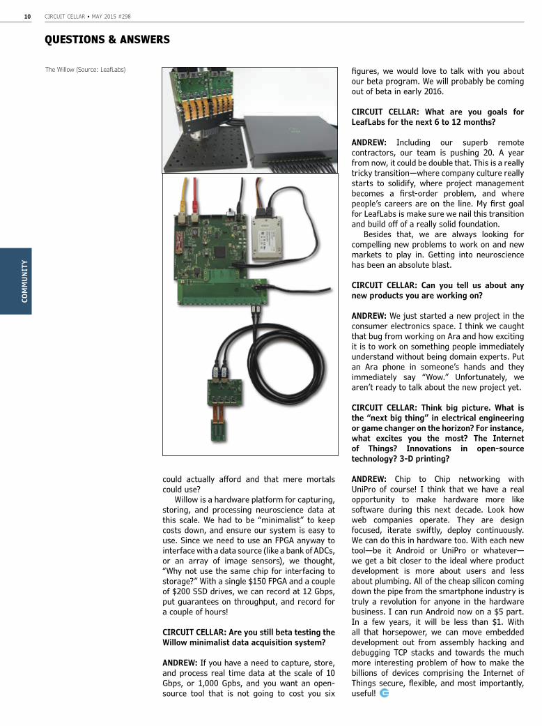
could actually afford and that mere mortals could use? Willow is a hardware platform for capturing, storing, and processing neuroscience data at this scale. We had to be “minimalist” to keep costs down, and ensure our system is easy to use. Since we need to use an FPGA anyway to interface with a data source (like a bank of ADCs, or an array of image sensors), we thought, “Why not use the same chip for interfacing to storage?” With a single $150 FPGA and a couple of $200 SSD drives, we can record at 12 Gbps, put guarantees on throughput, and record for a couple of hours!
CIRCUIT CELLAR: Are you still beta testing the Willow minimalist data acquisition system?
ANDREW: If you have a need to capture, store, and process real time data at the scale of 10 Gbps, or 1,000 Gpbs, and you want an open-source tool that is not going to cost you six
figures, we would love to talk with you about our beta program. We will probably be coming out of beta in early 2016.
CIRCUIT CELLAR: What are you goals for LeafLabs for the next 6 to 12 months?
ANDREW: Including our superb remote contractors, our team is pushing 20. A year from now, it could be double that. This is a really tricky transition—where company culture really starts to solidify, where project management becomes a first-order problem, and where people’s careers are on the line. My first goal for LeafLabs is make sure we nail this transition and build off of a really solid foundation. Besides that, we are always looking for compelling new problems to work on and new markets to play in. Getting into neuroscience has been an absolute blast.
CIRCUIT CELLAR: Can you tell us about any new products you are working on?
ANDREW: We just started a new project in the consumer electronics space. I think we caught that bug from working on Ara and how exciting it is to work on something people immediately understand without being domain experts. Put an Ara phone in someone’s hands and they immediately say “Wow.” Unfortunately, we aren’t ready to talk about the new project yet.
CIRCUIT CELLAR: Think big picture. What is the “next big thing” in electrical engineering or game changer on the horizon? For instance, what excites you the most? The Internet of Things? Innovations in open-source technology? 3-D printing?
ANDREW: Chip to Chip networking with UniPro of course! I think that we have a real opportunity to make hardware more like software during this next decade. Look how web companies operate. They are design focused, iterate swiftly, deploy continuously. We can do this in hardware too. With each new tool—be it Android or UniPro or whatever—we get a bit closer to the ideal where product development is more about users and less about plumbing. All of the cheap silicon coming down the pipe from the smartphone industry is truly a revolution for anyone in the hardware business. I can run Android now on a $5 part. In a few years, it will be less than $1. With all that horsepower, we can move embedded development out from assembly hacking and debugging TCP stacks and towards the much more interesting problem of how to make the billions of devices comprising the Internet of Things secure, flexible, and most importantly, useful!
The Willow (Source: LeafLabs)

Each month, you’re challenged to find an error in a schematic or in code that’s presented on the challenge
webpage. Locate the error for a chance to win prizes and recognition in Circuit Cellar magazine!
Prizes such as a NetBurner MOD54415 LC Development kit or a Circuit Cellar subscription will be announced each month.
MONTHLY
ENGINEERING CHALLENGE
Sponsored by NetBurner
Participate: circuitcellar.com/engineering-challenge-netburnerLaunch: 1st of each month
Deadline: 20th of each month
No purchase necessary to enter or win. Void where prohibited by law. Registration required. Prizes subject to change based on availability. Review these terms before submitting each Entry. More info: circuitcellar.com/engineering-challenge-netburner-terms
CIRCUIT CELLAR • MAY 2015 #29812
INDU
STRY
& E
NTER
PRIS
E
PRODUCT NEWS
OptiMOS PRODUCT FAMILY EXCEEDS 95% EFFICIENCYInfineon Technologies recently launched the OptiMOS 5 25-
and 30-V product family, the next generation of Power MOSFETs in standard discrete packages, a new class of power stages named Power Block, and in an integrated power stage, DrMOS 5×5. Together with Infineon’s driver and digital controller products the company delivers full system solutions for applications such as server, client, datacom or telecom.
The newly introduced OptiMOS family offers benchmark solutions with efficiency improvements of around 1% across the whole load range compared to its previous generation, exceeding 95% peak efficiency in a typical server voltage regulator design. This improved performance is based for example on the reduction of switching losses (Q switch) by 50% compared to the previous OptiMOS technology. Thus, implementing the new OptiMOS 25 V would lead to energy savings of 26.3 kWh per year for a single 130-W server CPU working 365 days.
The launch of the OptiMOS product family is accompanied by the introduction of a new packaging technology offering a further
reduction in PCB area consumption. It is used in the Power Block product family and in the integrated powerstage DrMOS 5×5 and offers a source down low-side MOSFET for improved thermal performance, with a reduction by 50% of the thermal resistance in comparison to standard package solution, such as SuperSO8.
Infineon’s Power Block is a leadless SMD package comprising the low-side and high-side MOSFET of a synchronous DC/DC converter into a 5.0 × 6.0 mm two-package outline. With Power Block, customers can shrink their designs up to 85 percent by replacing two separate discrete packages, such as SuperSO8 or SO-8. Both, the small package outline and the interconnection of the two MOSFETs within the package minimize the loop inductance for best system performance.
OptiMOS 5 25V is also used in an integrated power stage, combining DrMOS 5×5, driver and two MOSFETs, for a total area consumption on the PCB equal to 25 mm². The integrated driver plus MOSFETs solution results in a shorter design time and is easy to design-in. Additionally, the dovetailed power stage includes a high accurate temperature sense of +/-5°C (compared to +/-10°C of an external one) which enables higher system reliability and performance.
Samples of the new OptiMOS 25- and 30-V devices in SuperSO8, S3O8 and Power Block packages, with on-state resistances from 0.9 mΩ to 3.3 mΩ are available. Additional products with monolithic integrated Schottky-like diode and products in 30 V will be available from Q2 2015 onwards. DrMOS 5×5 will be released in Q2 2015. Samples are available.
Infineon Technologies | www.infineon.com
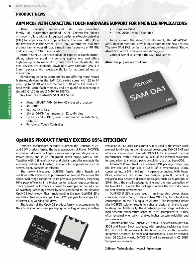
ARM MCUs WITH CAPACITIVE TOUCH HARDWARE SUPPORT FOR HMI & LIN APPLICATIONSAtmel recently announced its next-generation
family of automotive-qualified ARM Cortext-M0+-based microcontrollers with an integrated peripheral touch controller (PTC) for capacitive touch applications. The new SAM DA1 is the first series in this Atmel |SMART MCU automotive-qualified product family, operating at a maximum frequency of 48 MHz and reaching a 2.14 Coremark/MHz.
Atmel’s SAM DA1 series is ideal for capacitive touch button, slider, wheel or proximity sensing applications and offers high analog performance for greater front-end flexibility. The new devices are available down to a very compact QFN 5 × 5 mm package with wettable flanks for automated optical inspection.
Eliminating external components and offering more robust features, devices in the SAM DA1 series come with 32 to 64 pins, up to 64 KB of flash memory, 8 KB of SRAM, and 2-KB read-while-write flash memory and are qualified according to the AEC Q-100 Grade 2 (–40° to 105°C).
Key Features of Atmel’s SAM DA1 Series:
• Atmel |SMART ARM Cortex-M0+-based processor• 45 DMIPS• VCC 2.7 to 3.63 V• 16- to 64-KB flash memory; 32 to 64 pins• Up to six SERCOM (Serial Communication Interface),
USB, I2S• Peripheral Touch Controller
• Complex PWM• AEC Q100 Grade 2 Qualified
To accelerate the design development, the ATSAMDA1-XPRO development kit is available to support the new devices. The new SAM DA1 series is also supported by Atmel Studio, Atmel Software Framework and debuggers.
Contact Atmel to sample the SAM DA1 series.
Atmel Corp. | www.atmel.com
circuitcellar.com 13INDUSTRY &
ENTERPRISE
PRODUCT NEWS
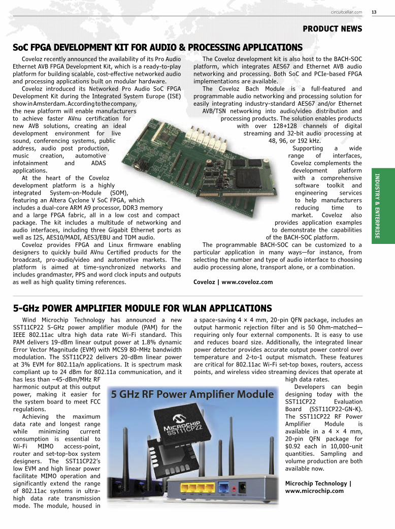
5-GHz POWER AMPLIFIER MODULE FOR WLAN APPLICATIONSWind Microchip Technology has announced a new
SST11CP22 5-GHz power amplifier module (PAM) for the IEEE 802.11ac ultra high data rate Wi-Fi standard. This PAM delivers 19-dBm linear output power at 1.8% dynamic Error Vector Magnitude (EVM) with MCS9 80-MHz bandwidth modulation. The SST11CP22 delivers 20-dBm linear power at 3% EVM for 802.11a/n applications. It is spectrum mask compliant up to 24 dBm for 802.11a communication, and it has less than –45-dBm/MHz RF harmonic output at this output power, making it easier for the system board to meet FCC regulations.
Achieving the maximum data rate and longest range while minimizing current consumption is essential to Wi-Fi MIMO access-point, router and set-top-box system designers. The SST11CP22’s low EVM and high linear power facilitate MIMO operation and significantly extend the range of 802.11ac systems in ultra-high data rate transmission mode. The module, housed in
a space-saving 4 × 4 mm, 20-pin QFN package, includes an output harmonic rejection filter and is 50 Ohm-matched—requiring only four external components. It is easy to use and reduces board size. Additionally, the integrated linear power detector provides accurate output power control over temperature and 2-to-1 output mismatch. These features are critical for 802.11ac Wi-Fi set-top boxes, routers, access points, and wireless video streaming devices that operate at
high data rates.Developers can begin
designing today with the SST11CP22 Evaluation Board (SST11CP22-GN-K). The SST11CP22 RF Power Amplifier Module is available in a 4 × 4 mm, 20-pin QFN package for $0.92 each in 10,000-unit quantities. Sampling and volume production are both available now.
Microchip Technology | www.microchip.com
SoC FPGA DEVELOPMENT KIT FOR AUDIO & PROCESSING APPLICATIONSCoveloz recently announced the availability of its Pro Audio
Ethernet AVB FPGA Development Kit, which is a ready-to-play platform for building scalable, cost-effective networked audio and processing applications built on modular hardware.
Coveloz introduced its Networked Pro Audio SoC FPGA Development Kit during the Integrated System Europe (ISE) show in Amsterdam. According to the company, the new platform will enable manufacturers to achieve faster AVnu certification for new AVB solutions, creating an ideal development environment for live sound, conferencing systems, public address, audio post production, music creation, automotive infotainment and ADAS applications.
At the heart of the Coveloz development platform is a highly integrated System-on-Module (SOM), featuring an Altera Cyclone V SoC FPGA, which includes a dual-core ARM A9 processor, DDR3 memory and a large FPGA fabric, all in a low cost and compact package. The kit includes a multitude of networking and audio interfaces, including three Gigabit Ethernet ports as well as I2S, AES10/MADI, AES3/EBU and TDM audio.
Coveloz provides FPGA and Linux firmware enabling designers to quickly build AVnu Certified products for the broadcast, pro-audio/video and automotive markets. The platform is aimed at time-synchronized networks and includes grandmaster, PPS and word clock inputs and outputs as well as high quality timing references.
The Coveloz development kit is also host to the BACH-SOC platform, which integrates AES67 and Ethernet AVB audio networking and processing. Both SoC and PCIe-based FPGA implementations are available.
The Coveloz Bach Module is a full-featured and programmable audio networking and processing solution for easily integrating industry-standard AES67 and/or Ethernet
AVB/TSN networking into audio/video distribution and processing products. The solution enables products
with over 128+128 channels of digital streaming and 32-bit audio processing at
48, 96, or 192 kHz.Supporting a wide
range of interfaces, Coveloz complements the development platform with a comprehensive software toolkit and engineering services to help manufacturers reducing time to
market. Coveloz also provides application examples
to demonstrate the capabilities of the BACH-SOC platform.
The programmable BACH-SOC can be customized to a particular application in many ways—for instance, from selecting the number and type of audio interface to choosing audio processing alone, transport alone, or a combination.
Coveloz | www.coveloz.com

CIRCUIT CELLAR • MAY 2015 #29814
INDU
STRY
& E
NTER
PRIS
E
PRODUCT NEWS
ONLINE CLASSROOM FOR ANALOG DESIGNTexas Instruments recently launched TI Precision Labs, which is
a comprehensive online classroom for analog engineers to take on-demand courses. The free, modular curriculum includes more than 30 training experiences and lab videos covering analog amplifier design considerations with online coursework.
TI Precision Labs incorporates a variety of tools to bring the online training experience to life. A $199 TI Precision Labs Op Amp Evaluation Module (TI-PLABS-AMP-EVM) enables engineers to complete each demonstrated learning activity along with the trainer. The curriculum also provides access to free design tools, such as TI Designs reference designs and TI’s TINA-TI SPICE model simulator.
Engineers can evaluate circuits and small-signal AC performance created during the trainings with National Instruments’s VirtualBench all-in-one instrument and TI’s Bode Analyzer Software for VirtualBench, as well as standard engineering bench equipment.
Key features and benefits of TI Precision Labs:
• Experiential learning applies theory to real-world, hands-on examples with lab demonstration videos.
• Customized learning environment • Accelerated learning for recent graduates focused on real-
world designing• Robust learning materials include a downloadable
presentation workbook and lab manual, as well as TI’s Analog Engineer’s Pocket Reference
• TI Precision Labs support forum is available on the TI E2E Community
The TI Precision Labs training curriculum is free to anyone with a myTI account. In addition to free training, other benefits of myTI registration include the ability to purchase TI integrated circuits (ICs), evaluation modules, development kits and software; request product samples; get technical assistance through the TI E2E Community; create, simulate and optimize systems in the WEBENCH Design Center; and more.
TI Precision Labs curriculum is housed in the new TI Training Center, which connects engineers with the technical training they need to find solutions to their design challenges anytime, anywhere.
Texas Instruments | www.ti.com
5-V QI LOW-POWER WIRELESS CHARGING TRANSMITTER REFERENCE DESIGNNXP Semiconductors has announced the availability of a
new reference design for 5-V low-power Qi wireless charging transmitters, compliant with the Wireless Power Consortium (WPC) 1.1 Qi specification. The design is based on NXPs single-chip 5-V wireless power transmitter IC—the NXQ1TXA5 that was launched in 2014. It is the latest addition to NXP’s portfolio of Greenchip power solutions.
Building on NXP’s success as the market leader in Greenchip power ICs, the NXQ1TXA5 reference design has an unrivaled standby power consumption of less than 10 mW. It is the only solution on the market today that meets five-star mobile phone charger standby power ratings by consuming less than 30 mW in standby mode, which includes the standby power of the wall-charger. NXP recommends combining its NXQ1TXA5 ultra low standby power wireless power transmitter solution with another Greenchip device, its high efficiency TEA1720 SMPS IC with a standby power of less than 20 mW.
The NXQ1TXA5 device combines:
• NXPs patented high efficiency Class D amplifier technology for outstanding EMI performance.
• NXP’s ultra low power CoolFluxTM DSP technology for superior communication with smartphones placed on the charger.
• Dedicated low power mixed signal circuitry to check for smartphone presence three times per second, enabling fast startup of charging, while keeping the standby power very low if there is no smartphone on the charger.
Due to the NXQ1TXA5’s low-power consumption, the reference design also has a high efficiency for low transmitted powers, making it suitable for applications ranging from smartphone charging to deliver 5 W to the smartphone battery when used with a Qi compliant wireless charging receiver, to chargers for wearables that need less than 2-W charging power.
The NXQ1TXA5 reference design needs only 15 to 20 low-cost passive components and uses a standard two-layer PCB, with the components mounted on a single side. Depending on customer requirements, the complete application can be designed on a board space as small as 3 × 3 or 4 × 4 cm.
The new NXQ1TXA5 wireless charging transmitter reference design will be available in Q2.
NXP Semiconductors | www.nxp.com

circuitcellar.com 15
CLIENT PROFILEINDUSTRY &
ENTERPRISE
FEATURED PRODUCTSSince 1980, companies spanning a wide range of industries
have trusted LSR to help develop solutions that exceed their customers’ expectations. LSR provides an unmatched suite of both embedded wireless products and integrated services that improve speed to market and return on your development investment.
LSR’s SaBLE-x Bluetooth Smart module, based on TI’s new SimpleLink CC2640 MCU, offers industry-leading RF and power performance along with LSR’s renowned support and developer tools.
LSR’s TiWi-C-W is a stand-alone WLAN (IEEE 802.11 b/g/n) module that simplifies and accelerates the work
of adding Wi-Fi connectivity to your products. The TiWi-C-W module is also a cloud agent for LSR’s end-to-end IoT platform, TiWiConnect.
cc-webshop.com
Circuit Cellar 2014Digital Archive
With this digital subscription, you have access to all 12 issues of Circuit Cellar 2014 from any computer or tablet at anytime. Readers can explore project ideas, bookmark pages, and make annotations throughout each issue.
Circuit Cellar 2014 CDCD includes 12 issues of Circuit Cellar in PDF format along with related article code.
Order yours today
LS ResearchLocation: Cedarburg, WI, USAWeb: www.lsr.comContact: Dave Burleton ([email protected])
WHY SHOULD CC READERS BE INTERESTED? LSR’s all-new SaBLE-x Bluetooth Smart module, based on
TI’s new SimpleLink CC2640 MCU, offers industry-leading RF and power performance along with LSR’s renowned developer support and broad country certifications. The SaBLE-x can be utilized in either stand-alone mode or with an external host, and the SaBLE Tool Suite provides developers with intuitive tools that accelerates development time in integrating BLE into your products.
SPECIAL OFFER FROM LSRWin a FREE Development Kit for the SaBLE-x Bluetooth Smart
module! Register to win and ONE Circuit Cellar reader will receive LSR’s SaBLE-x Development Kit ($199 value). Go to: http://info.lsr.com/sable-x-exclusive-offer
Circuit Cellar prides itself on presenting readers with information about innovative companies, organizations, products, and services relating to embedded technologies. This space is where Circuit Cellar enables clients to present readers useful information, special deals, and more.
CIRCUIT CELLAR • MAY 2015 #29816FE
ATUR
ES
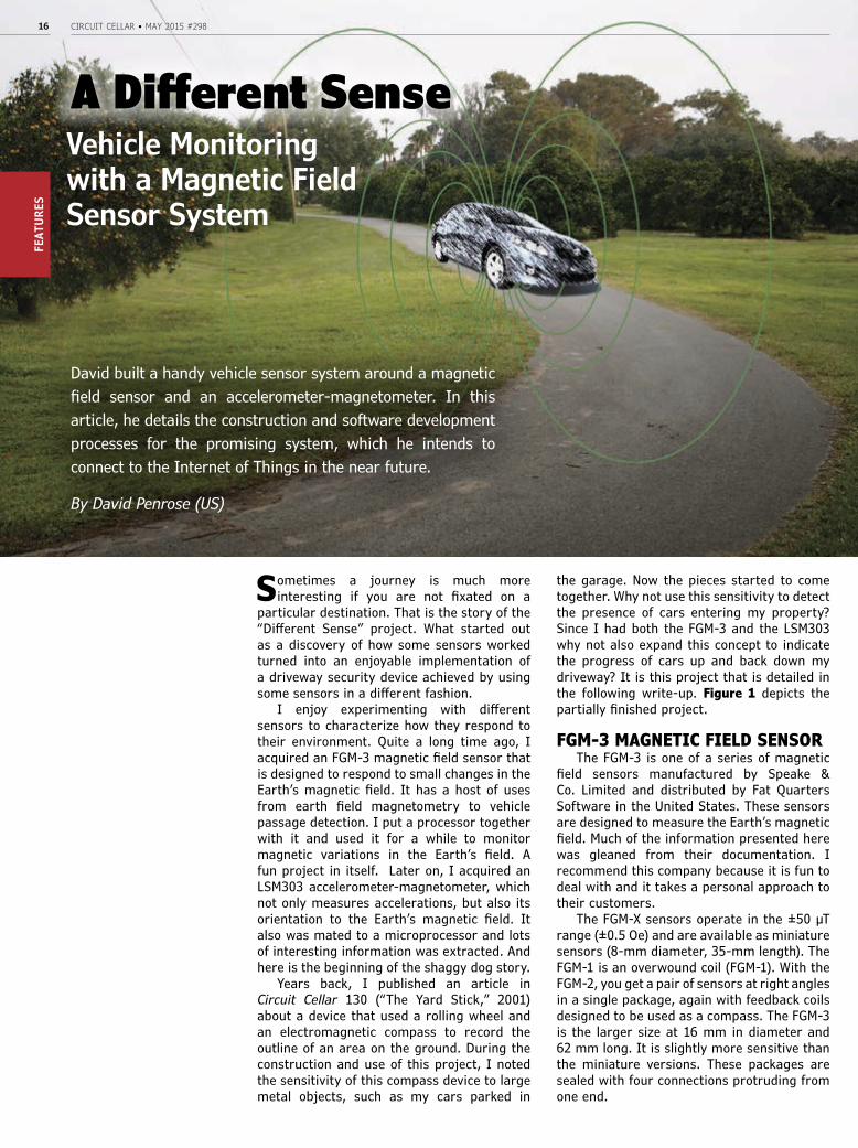
Sometimes a journey is much more interesting if you are not fixated on a
particular destination. That is the story of the “Different Sense” project. What started out as a discovery of how some sensors worked turned into an enjoyable implementation of a driveway security device achieved by using some sensors in a different fashion.
I enjoy experimenting with different sensors to characterize how they respond to their environment. Quite a long time ago, I acquired an FGM-3 magnetic field sensor that is designed to respond to small changes in the Earth’s magnetic field. It has a host of uses from earth field magnetometry to vehicle passage detection. I put a processor together with it and used it for a while to monitor magnetic variations in the Earth’s field. A fun project in itself. Later on, I acquired an LSM303 accelerometer-magnetometer, which not only measures accelerations, but also its orientation to the Earth’s magnetic field. It also was mated to a microprocessor and lots of interesting information was extracted. And here is the beginning of the shaggy dog story.
Years back, I published an article in Circuit Cellar 130 (“The Yard Stick,” 2001) about a device that used a rolling wheel and an electromagnetic compass to record the outline of an area on the ground. During the construction and use of this project, I noted the sensitivity of this compass device to large metal objects, such as my cars parked in
the garage. Now the pieces started to come together. Why not use this sensitivity to detect the presence of cars entering my property? Since I had both the FGM-3 and the LSM303 why not also expand this concept to indicate the progress of cars up and back down my driveway? It is this project that is detailed in the following write-up. Figure 1 depicts the partially finished project.
FGM-3 MAGNETIC FIELD SENSORThe FGM-3 is one of a series of magnetic
field sensors manufactured by Speake & Co. Limited and distributed by Fat Quarters Software in the United States. These sensors are designed to measure the Earth’s magnetic field. Much of the information presented here was gleaned from their documentation. I recommend this company because it is fun to deal with and it takes a personal approach to their customers.
The FGM-X sensors operate in the ±50 µT range (±0.5 Oe) and are available as miniature sensors (8-mm diameter, 35-mm length). The FGM-1 is an overwound coil (FGM-1). With the FGM-2, you get a pair of sensors at right angles in a single package, again with feedback coils designed to be used as a compass. The FGM-3 is the larger size at 16 mm in diameter and 62 mm long. It is slightly more sensitive than the miniature versions. These packages are sealed with four connections protruding from one end.
A Different Sense
David built a handy vehicle sensor system around a magnetic field sensor and an accelerometer-magnetometer. In this article, he details the construction and software development processes for the promising system, which he intends to connect to the Internet of Things in the near future.
By David Penrose (US)
Vehicle Monitoring with a Magnetic Field Sensor System
circuitcellar.com 17FEATURES
The FGM-3 also comes in an FGM-3h version, which has approximately 2.5× the sensitivity of the FGM-3. Its dynamic range is ±0.15 Oe, or one-third the field strength of the Earth’s magnetic field. The overwound coil may be used to create a bias and hence null out the ambient field. This allows very small variations in the magnetic field to be sensed even with the “background noise” of the Earth’s field. The datasheet recommends orienting the sensors in an east-west direction to stay within the linear range of the sensor. I was tempted to try this sensor, only the extra work to null the Earth’s field was a bit more than I wanted to undertake.
All of these sensors operate at a nominal voltage of 5 V and produce a pulsed output with a range of about 5 to 23 µs. This pulse-width period is measured over an input range of about –0.8 to 0.8 Oe with lower (or negative) Oersted producing the smaller periods (and higher frequencies). The nonlinearity is about 5% in the –0.5 to 0.5 Oe range and the readings are very sensitive to both voltage and temperature.
A number of interesting articles have been published (http://www.fatquarterssoftware.com/links.html) that detail the use of these devices to measure the variations in the Earth’s magnetic field due to space weather and other anomalies. My original experimentation was aimed at recreating some of these results and were fairly successful. It was at this point that the story progresses to the semiconductor relatives of these devices.
SEMICONDUCTOR MAGNETOMETER
The FGM-X sensors are not inexpensive ($50 to $60), and it will be interesting to see how they compete against semiconductor sensors such as the LM303 and more recent versions of this device. I acquired a few samples of these sensors to experiment with their capability of producing tilt-compensated compass readings. The sensors provide a combination reading of the Earth magnetic field together with the acceleration due to gravity. If you have experimented with earlier electronic compasses such as the field-gate type, you will recognize the significant error introduced in the magnetic reading if the device is not perfectly horizontal. Some of the earlier electronic compasses (and most high end magnetic compasses) used gimbals to keep the sensing coils (or magnetic needle) horizontal and hence reduce the effect of pitch and roll. The new semiconductor sensors provide readouts of both the magnetic and gravitational fields from one package where these axes are locked together. The higher-end devices even include processing to use these
measurements to produce a compensated direction indicator. The less expensive devices such as the LM303 just generate the raw outputs and leave the processing to an external microprocessor.
What the semiconductor devices gain in cost and micro-packaging, they give up in sensitivity. The LM303 produces a 16-bit output on its I2C interface and has a total range of ±2 Gs minimum (selectable from ±2, ±4, ±8, and ±12), which yields a 0.08 mGs/LSB. The translation from gauss to tesla is as follows: 1 Gs = 0.0001 T. The ±50 µT full range from the FGM-3 looks a bit better than the LM303. Nevertheless, my intent was not to measure small variations in the Earth’s magnetic field over time, but to just tilt compensate the compass reading so this sensitivity was fine. This process of combining the accelerometer and magnetometer readings
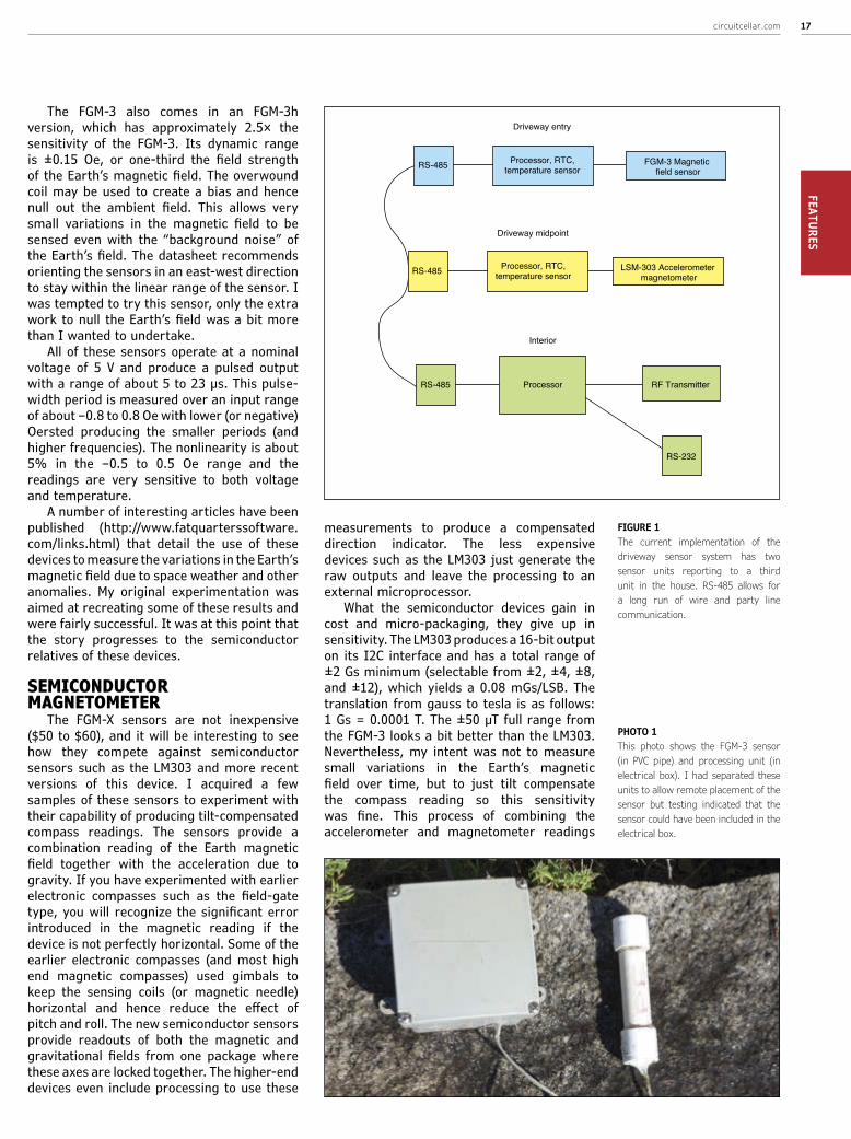
PHOTO 1 This photo shows the FGM-3 sensor (in PVC pipe) and processing unit (in electrical box). I had separated these units to allow remote placement of the sensor but testing indicated that the sensor could have been included in the electrical box.
FIGURE 1 The current implementation of the driveway sensor system has two sensor units reporting to a third unit in the house. RS-485 allows for a long run of wire and party line communication.
Driveway entry
RS-485 Processor, RTC,temperature sensor
FGM-3 Magnetic field sensor
Driveway midpoint
RS-485 Processor, RTC,temperature sensor
LSM-303 Accelerometer magnetometer
Interior
RS-485
RS-232
Processor RF Transmitter
CIRCUIT CELLAR • MAY 2015 #29818FE
ATUR
ES
is straightforward but not trivial. It involves geometric relationships and there is a bit of trigonometry involved with floating-point numbers required for the highest accuracy and flexibility. My challenge with this device became producing a compensated compass reading from a low-end, 8-bit microprocessor running at modest speed. This was an interesting pursuit and was successful. I’ll probably return to this work later but now my journey had drifted off course again and I began thinking of using the semiconductor device as an inexpensive detector of vehicles. This new application avoided all the software involved in computing the true heading but
instead just used the raw magnetic data from the device.
HARDWARE IMPLEMENTATIONThe earlier work with FGM-3 used a
microprocessor, a real-time clock, and a temperature sensor to measure the reported field strength and correlate it to time and temperature. These values were reported over an RS-485 interface to give me the option to place the device well outside my house and still generate an error-free message at a fairly high rate. This basic architecture was also suitable, if not overkill, for my new destination of sensing vehicles and reporting on their passage. Photo 1 shows the completed package for the FGM-3 sensor. I constructed a second hardware set for the LM303 and was in business.
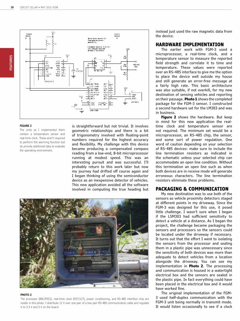
Figure 2 shows the hardware. But keep in mind for this new application the real-time clock and temperature sensor are not required. The minimum set would be a microprocessor, an RS-485 chip, the sensor, and some sort of power regulation. One word of caution depending on your selection of RS-485 devices: make sure to include the line termination resistors as indicated in the schematic unless your selected chip can accommodate an open line condition. Without this termination an open line such as when both devices are in receive mode will generate erroneous characters. The line termination resistors eliminate these problems.
PACKAGING & COMMUNICATIONMy new destination was to use both of the
sensors as vehicle proximity detectors staged at different points in my driveway. Since the FGM-3 was designed for this use, it posed little challenge. I wasn’t sure when I began if the LSM303 had sufficient sensitivity to detect a vehicle at a distance. As I began the project, the challenge became packaging the sensors and processors so the sensors could be located under the driveway if necessary. It turns out that the effort I went to isolating the sensors from the processor and sealing them in a plastic pipe was unnecessary since the sensitivity of both devices was more than adequate to detect vehicles from a location alongside the driveway. You can see my implementation in Photo 2. The processing and communication is housed in a watertight electrical box and the sensors are sealed in the plastic pipe. In fact everything could have been placed in the electrical box and it would have worked fine.
The original implementation of the FGM-3 used half-duplex communication with the FGM-3 unit being normally in transmit mode. It would listen occasionally to see if a clock
PHOTO 2The processor (89LCP922), real-time clock (PCF2127), power conditioning, and RS-485 interface chip are visible in this photo. I distribute 12 V over one pair of a two pair RS-485 communication cable and regulate it to 3.3 V and 5 V on the board.
FIGURE 2 The units as I implemented them contain a temperature sensor and real-time clock. These aren’t required to perform the alarming function but do provide additional data to evaluate the operating environment.

CIRCUIT CELLAR • MAY 2015 #29820FE
ATUR
ES
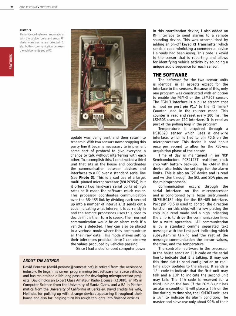
update was being sent and then return to transmit. With two sensors now occupying this party line it became necessary to implement some sort of protocol to give everyone a chance to talk without interfering with each other. To accomplish this, I constructed a third unit that sits in the house and coordinates the communication between devices and interfaces to a PC over a standard serial line (see Photo 3). This is a sad use of a large, multi-pinned microprocessor (89LPC954), but it offered two hardware serial ports at high rates so it made the software much easier. This processor coordinates communication over the RS-485 link by dividing each second up into a number of intervals. It sends out a code indicating what interval it is currently in and the remote processors uses this code to decide if it is their turn to speak. Their normal communication would be an alarm code if a vehicle is detected. They can also be placed in a verbose mode where they communicate all their raw data. This mode makes setting their tolerances practical since I can observe the values produced by vehicles passing.
Since I had a lot of unused computer power
in this coordination device, I also added an RF interface to send alarms to a remote sounding device. This was accomplished by adding an on-off keyed RF transmitter which sends a code mimicking a commercial device I already had been using. This code is keyed to the sensor that is reporting and allows for identifying vehicle activity by sounding a unique audio sequence for each sensor.
THE SOFTWAREThe software for the two sensor units
is identical in all aspects except for the interface to the sensors. Because of this, only one program was constructed with an option to enable the FGM-3 or the LSM303 sensor. The FGM-3 interface is a pulse stream that is input on port pin P1.7 to the T1 Timer/Counter used in the counter mode. This counter is read and reset every 100 ms. The LSM303 uses an I2C interface. It is read as part of the polling loop in the program.
Temperature is acquired through a DS18B20 sensor which uses a one-wire interface, which is tied to pin P0.6 on the microprocessor. This device is read about once per second to allow for the 750-ms acquisition phase of the sensor.
Time of day is maintained in an NXP Semiconductors PCF2127T real-time clock chip with battery back-up. The RAM in this device also holds the settings for the alarm limits. This is also an I2C device and is read and written through the SCL and SDA pins on the microprocessor.
Communication occurs through the serial interface on the microprocessor and is conditioned by a Texas Instruments SN75LBC184 chip for the RS-485 interface. Port pin P0.5 is used to control the direction function on this chip, with a low placing the chip in a read mode and a high indicating the chip is to drive the communication lines for a write operation. All communication is by a standard comma separated text message with the first part indicating which subsystem is talking and the rest of the message communication the sensor values, the time, and the temperature.
The controller software in the processor in the house sends an 11h code on the serial line to indicate that it is talking. It may use this time slot to send configuration or real-time clock updates to the slaves. It sends a 12h code to indicate that the first unit may talk and a 13h to indicate the second unit may talk. The 14h code is reserved for a third unit on the bus. If the FGM-3 unit has an alarm condition it will place a 15h on the line during its time slot, the LSM303 unit uses a 16h to indicate its alarm condition. The master and slave use only about 90% of their
PHOTO 3This unit coordinates communications with the outdoor units and sends RF alerts when alarms are detected. It also buffers communication between the outdoor units and a PC.
ABOUT THE AUTHORDavid Penrose ([email protected]) is retired from the aerospace industry. He began his career programming test software for space vehicles and has maintained a life-long passion for developing microprocessor proj-ects. David holds an Expert Class Amateur Radio License (K1DHP), an MS in Computer Science from the University of Santa Clara, and a BA in Mathe-matics from the University of California at Berkeley. David credits his wife, Melinda, for putting up with strange devices appearing throughout their house and also for helping turn his rough thoughts into finished articles.
circuitcellar.com 21FEATURES
time slot and if they are not listening when their allocation arrives will wait for the next cycle prior to communicating to ensure their message will fit in one time slot.
THE RESULTSThe FGM-3 sensor is so sensitive that it
can easily detect the passage of vehicles 20´ from the sensor. Large trucks passing by in the street can trigger this sensor. I can set the sensitivity of the unit to ignore these events and alarm only on close by vehicles. The LSM303 unit is at the half-way point in the driveway and easily generates reliable alarms when a vehicle is within about 10 . When I first placed the units, I enabled the verbose mode and used this to set the alarming conditions. The first observation was that the units behaved differently over time. The FGM-3 readings would slowly vary throughout the day so the conditions for its alarms had to use a moving average as a starting point and then alarm when significant excursions were noticed. The LSM303, on the other hand, was stable throughout the day but was noisier. I used a simple averaging to eliminate this noise and get a reliable floor. Moving the sensors changes the nominal values but the excursion testing for the alarms still work reliably.
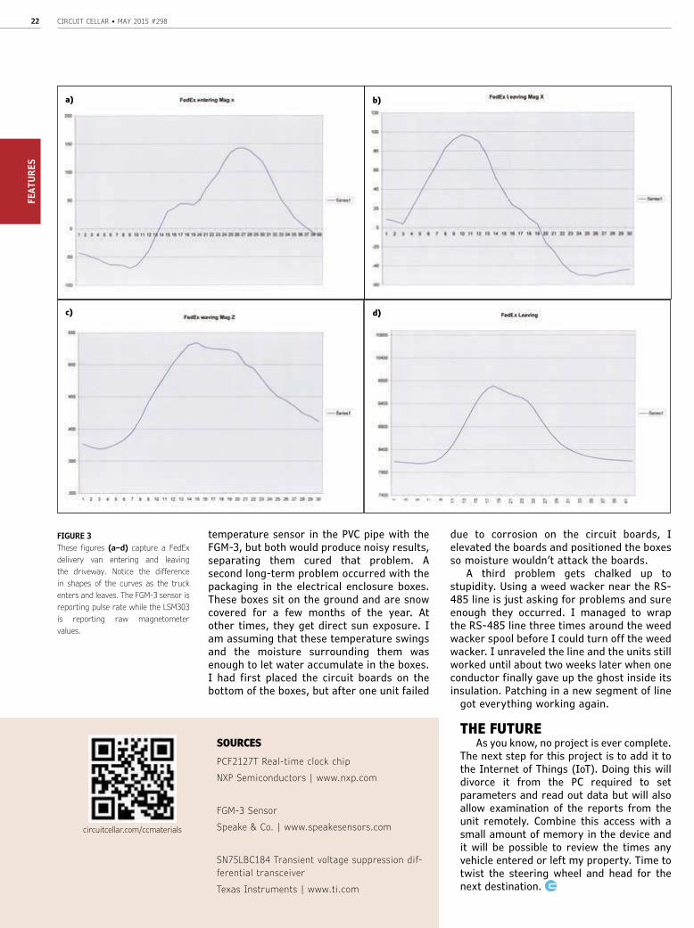
Using the verbose mode, I recorded a number of samples generated by both sensors when a FedEx truck made a delivery. This data is plotted and presented in Figures 3a–d. Figure 3a capture the response of the x-axis magnetometer (LM303) for the truck entering the driveway, while Figure 3b shows it leaving. Figure 3c shows the z-axis for the truck leaving the driveway. The data from the FGM-3 sensor is shown in figure 3d for the truck leaving. Notice the difference in the response curves for the LM303 sensor as the truck enters and leaves the driveway. I haven’t tried to use this difference yet to generate an entering or leaving alarm but that is in the future. The alarm logic for the LSM303 checks all three axes for perturbations, but it requires only one to exceed its tolerances to issue an alarm. This feature allows the sensor to be placed at any orientation and still function.
Both sensors have been in use for about two years and much has been learned on packaging for the real world, but they both continue to produce very valid data on vehicle traffic entering and leaving my property. One of the first lessons learned was the FGM-3 and the temperature sensor did not like to be near each other. I had originally located the
CIRCUIT CELLAR • MAY 2015 #29822FE
ATUR
ES
temperature sensor in the PVC pipe with the FGM-3, but both would produce noisy results, separating them cured that problem. A second long-term problem occurred with the packaging in the electrical enclosure boxes. These boxes sit on the ground and are snow covered for a few months of the year. At other times, they get direct sun exposure. I am assuming that these temperature swings and the moisture surrounding them was enough to let water accumulate in the boxes. I had first placed the circuit boards on the bottom of the boxes, but after one unit failed
due to corrosion on the circuit boards, I elevated the boards and positioned the boxes so moisture wouldn’t attack the boards.
A third problem gets chalked up to stupidity. Using a weed wacker near the RS-485 line is just asking for problems and sure enough they occurred. I managed to wrap the RS-485 line three times around the weed wacker spool before I could turn off the weed wacker. I unraveled the line and the units still worked until about two weeks later when one conductor finally gave up the ghost inside its insulation. Patching in a new segment of line
got everything working again.
THE FUTUREAs you know, no project is ever complete.
The next step for this project is to add it to the Internet of Things (IoT). Doing this will divorce it from the PC required to set parameters and read out data but will also allow examination of the reports from the unit remotely. Combine this access with a small amount of memory in the device and it will be possible to review the times any vehicle entered or left my property. Time to twist the steering wheel and head for the next destination.
circuitcellar.com/ccmaterials
SOURCESPCF2127T Real-time clock chip
NXP Semiconductors | www.nxp.com
FGM-3 Sensor
Speake & Co. | www.speakesensors.com
SN75LBC184 Transient voltage suppression dif-ferential transceiver
Texas Instruments | www.ti.com
FIGURE 3These figures (a–d) capture a FedEx delivery van entering and leaving the driveway. Notice the difference in shapes of the curves as the truck enters and leaves. The FGM-3 sensor is reporting pulse rate while the LSM303 is reporting raw magnetometer values.
a) b)
c) d)

Design with the ahead of their time.
You can’t invent the future with products from the past.
Authorized global distributor of the NEWEST electronic components.
Mouser and Mouser Electronics are registered trademarks of Mouser Electronics, Inc. Other products,
logos, and company names mentioned herein, may be trademarks of their respective owners.
C
M
Y
CM
MY
CY
CMY
K
Mouser_FutureProducts_Ci rcui tCel lar_5-1.pdf 1 3/18/15 1:02 PM
CIRCUIT CELLAR • MAY 2015 #29824FE
ATUR
ES
Some time ago, I ran across an inexpensive humidity sensor, the DHT11, for under
$2 each. I thought it would be interesting to experiment with it. After I got it working, I thought it might be interesting to compare it against a name-brand humidity sensor, so I added a Honeywell Humidicon sensor to the same circuit and compared the results.
Why would you want to build your own humidity measurement circuit? You can buy humidity gauges at a discount store, right? I did it because I thought it was an interesting experiment. But, as a practical matter, you might want to log the humidity variations in your house through a 24-hour day. A person with health issues related to very dry air might want to know how the humidity varied overnight while they were sleeping. You might want to log the humidity in a greenhouse, humidity-controlled storage area, or in a basement where the humidity is uncontrolled but maybe woodwind musical instruments can be damaged if it gets too low.
WHAT IS RELATIVE HUMIDITY?The first thing to understand about a
humidity sensor is what it’s actually measuring. Electronic humidity sensors typically measure relative humidity (RH), which is the ratio of water vapor in the air to the amount of water vapor in the air that would start condensing as liquid. The relative humidity is dependent on temperature; at higher temperatures,
more water can exist as vapor per cubic foot than at lower temperatures. For those of us who wear glasses, this is why our glasses fog up when we come inside after shoveling the snow; the warm inside air turns cold when it hits the cold glasses. The water vapor in the warmer air can’t stay in vapor form at the lower temperature, so the moisture condenses on the cold surface. Since relative humidity is temperature-dependent, electronic humidity sensors typically provide temperature information as well. The sensor needs to know the temperature to measure humidity, so a temperature sensor has to be included.
Humidity also varies with pressure, but most of the time when we measure humidity, we aren’t concerned with that variable. Wikipedia has a detailed article describing relative humidity.
HUMIDITY SENSORS AT WORKSensing relative humidity electronically
has been a challenge in the past. I remember years ago finding a humidity sensor in a box of surplus equipment. It was a box with a stack of high-quality PC boards with gold-plated traces in an interlocking pattern. The entire thing was about 3 inches square by maybe five inches long. That didn’t include any of the electronics to actually take measurements from it. These sensors work by measuring the change in the dielectric of the base PCB as it
Comparing Humidity SensorsStuart recently tested the efficacy of an inexpensive humidity sensor against a brand-name sensor in the same circuit. In this article, after explaining how humidity sensors work, he presents the results from his experiment.
By Stuart Ball (US)
circuitcellar.com 25FEATURES
absorbs moisture from the air. The dielectric change causes a capacitance change between the electrodes.
The DHT11 and the Honeywell Humidicon sensor are CMOS humidity sensors. These sensors work on the same principle as the old PCB sensor I encountered, but the dielectric and the electrode elements are part of the measurement IC. This allows the device to avoid many of the aging issues of older sensors, and the sensor calibration can be incorporated into the sensing circuitry.
The DHT11 sensor is about 0.5” × 0.6”, and has an accuracy of ±5% over the range of 20% to 80% RH. It uses a 40-bit serial interface to transmit the temperature and humidity information. The actual sensor element is smaller than the plastic enclosure.
The Honeywell Humidicon sensor was a Honeywell HIH6120-021-001. It is smaller than the DHT11, about 0.15” × 0.2”. This sensor has an accuracy of ±4% and a measurement range of 10% to 90% RH. The Humidicon is in a four-pin SIP package, with pins on 0.05” centers, and has an I2C interface. The same sensor is also available in a SOIC package, which can have either the I2C or SPI interface. You can’t get the SIP version with the SPI interface; there aren’t enough pins.
Both sensors provide temperature in degrees Celsius and relative humidity, and both can operate with supply voltages up to 5 V. Since the DHT11 has pins on 0.1” spacing, it is easier to connect when using a prototype board.
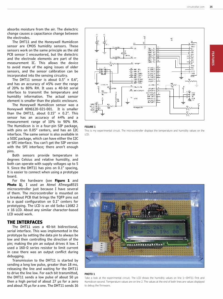
For the hardware (see Figure 1 and Photo 1), I used an Atmel ATmega8515 microcontroller just because I have several of them. The microcontroller is mounted on a breakout PCB that brings the TQFP pins out to a quad configuration on 0.1” centers for prototyping. The LCD is an old Seiko L1682 2 × 16 LCD. About any similar character-based LCD would work.
THE INTERFACESThe DHT11 uses a 40-bit bidirectional,
serial interface. This was implemented in the prototype by setting the data pin to always be low and then controlling the direction of the pin; making the pin an output drives it low. I used a 160-Ω series resistor to limit current in case there was an output conflict during debugging.
Transmission to the DHT11 is started by sending a long low pulse, greater than 18 ms, releasing the line and waiting for the DHT11 to drive the line low. For each bit transmitted, the DHT11 sends a low pulse of about 50 µs then a high period of about 27 µs for a zero and about 70 µs for a one. The DHT11 sends 16
PHOTO 1Take a look at the experimental circuit. The LCD shows the humidity values on line 1—DHT11 first and Humidicon second. Temperature values are on line 2. The values at the end of both lines are values displayed to debug the firmware.
FIGURE 1This is my experimental circuit. The microcontroller displays the temperature and humidity values on the LCD.

CIRCUIT CELLAR • MAY 2015 #29826FE
ATUR
ES
bits each for the temperature and humidity, but only the most significant byte of each value is used. A checksum byte is sent at the end of the transmission so the transmission can be verified. The DHT11 humidity and temperature values are transmitted in percent RH and degrees Celsius; no conversion of the values is required.
The bit timing is performed in firmware on the prototype and the low pulse time is used as a reference for the one/zero threshold. This method eliminates the need for the a fixed one/zero threshold that has to change with the microcontroller clock, but it depends on the loop timing for measuring the high and low bit times to be about the same. It also forces the software to be dedicated to receiving the DHT11 data while that is occurring.
If you wanted to use interrupts in the system, then you would want to measure the bit timing with a free-running counter or read the background timer interrupt or do something similar. You would need something that provides a fixed timing reference.
The Humidicon I2C interface is also implemented in software. To read humidity and temperature, the host sends the Humidicon an I2C write command, waits about 40 ms, then sends a read command and reads the data. If an I2C NACK is sent after the humidity is read, then the
temperature is not read. Or, an ACK can be sent and the humidity value will be followed by the temperature. I captured both in the prototype because I wanted to compare the temperature on the two sensors as a sanity check on the data.
The Humidicon sends 14-bit temperature and humidity values, but I only used the upper 8 bits of each. The Humidicon requires a conversion from the value read to humidity percentage and temperature in degrees Celsius. This is explained in Honeywell’s 2012 technical note, “I2C Communication with the Honeywell HumidIcon Digital Humidity/Temperature Sensors.” The technical note is available on the Honeywell website.
Both interfaces were implemented in software by driving and sampling the microcontroller pins. The DHT11, of course, had to be implemented this way because it is a nonstandard interface.
The Humidicon can measure temperature from –25° to 85°C. The compensated range (the range for which the humidity is calibrated to temperature) is 5° to 50°C. The DHT11 temperature range is 0 to 50°C. Since my goal was to compare the two humidity sensors (not temperature), the firmware doesn’t handle negative temperature values from the Humidicon. It wouldn’t be hard to add this by sign-extending the 14-bit value and treating it as a signed integer.
COMPARISONI compared the two sensors by moving
the prototype to various parts of the house, allowing the readings to settle, and then looking at the result. I also measured them on different days when the furnace was running more or running less. I did all this during cooler weather in Colorado, where it tends to be fairly dry. To get the higher humidity readings, I put the circuit in a clear plastic box with a wet paper towel and then let everything stabilize. I then let the water slowly evaporate and recorded readings as the humidity fell.
The temperature readings of both sensors were consistently within 2°C of each other. I might have seen more numerical variation if they were measuring degrees Fahrenheit since the Fahrenheit scale has more resolution per degree (180° between freezing and boiling versus 100 for degrees Celsius). But in degrees Celsius, they tracked closely. This is an important consideration since relative humidity is dependent on temperature, so the RH reading is a function of the accuracy of both the humidity sensor and the temperature sensor.
When comparing humidity readings, the first thing I noticed is that the Humidicon
0
10
20
30
40
50
60
70
RH
Honeywell Humidicon vs DHT11
Humidicon
DHT11
FIGURE 2Here you see the DHT11 humidity readings compared to the Humidicon part. The DHT11s level off around 25%. Above that point, they tracked reasonably well, with some divergences.
circuitcellar.com 27FEATURES
sensor responds faster than the DHT11, especially when the humidity is rising. It is slower when humidity is falling, but still faster than the DHT11. Both sensors have specified response times around 6 s. The Humidicon datasheet lists the response time. The DHT11 lists response time to 1/e (63%) of final value. This obviously implies an exponential curve. But when the humidity suddenly increases (such as when putting it in the container to measure higher humidity levels), the Humidicon ramped toward the final value and stabilized faster than the DHT11. Of course, in most humidity measurement applications, humidity doesn’t change very fast so this isn’t an issue. But it’s something to keep in mind, as the following example illustrates.
If you are just measuring humidity, the speed of the sensor is probably irrelevant. But if you are controlling humidity, it may be more of an issue. As with any feedback control system, the ability of the sensor to measure changes in whatever you are controlling affects the control system design.
Imagine a relatively small enclosure such as a cabinet to keep woodwind instruments or collectible books at a specific humidity level. If the humidity control is performed with an on-off control, such as a water valve feeding an evaporative system, a slow sensor may cause a lot of overshoot in the humidity level. To compensate for this, you would need a faster sensor, finer control of the water feed (something more than an on/off valve) or a more sophisticated control algorithm. And the control algorithm will probably need to work with the cabinet mostly empty or mostly full. You don’t want to rewrite the firmware every time you buy a new instrument or a new book.
The point is that the speed of the sensor can either be very important or it can be ignored, depending on how you are using it. But the speed of the sensors is potentially a factor in the design of a control system.
The smaller range of the DHT11 (20%–80% RH) compared to the Humidicon (10%–90% RH) showed up in the lower range of humidity values. The DHT11 is specified to operate from 20% to 80% RH, but I found that it really leveled off below about 25%. The lowest reading I saw on the DHT11 was 23%, but it wasn’t at the lowest humidity I measured. Below 25% or so, the DHT11 values didn’t seem to correlate well with anything.
Of course, the obvious question is, how do I know it’s the DHT11 that’s wrong? I checked it by making some outside measurements with the prototype and comparing to the current humidity from a couple of weather sites on the Internet. Humidity varies from place to place within a local region, just like
temperature does, but the Humidicon was closer to the “official” humidity. In one case, the weather-station humidity was 16%, the Humidicon read 13%, which is well within the measurement accuracy of the sensor and the expected variation from the “official” number. This is outside the DHT11 measurement range, but it did indicate that the Humidicon is reasonably accurate compared to an external standard.
I did notice that the DHT11 seems to vary more. It appears to be less stable than the Humidicon. There were a number of humidity readings on the Humidicon that resulted in different readings for the DHT11. However, in all cases, the readings were within the tolerance of the sensors.
Figure 2 shows the comparison of RH readings of the two sensors across the range I measured. The chart has some rise at the end because I didn’t record every 1% humidity value above 50%. As you can see, at the low end, the DHT11 levels off around 25%. The unit I had didn’t quite reach the specified 20% range. Overall, they tracked reasonably well. Where they diverged it would be hard to tell which is more accurate without a calibrated reference.
ARDUINOLibraries for both sensors are available
for the Arduino. I obviously didn’t use the Arduino for prototyping. I actually used a prototype board that I originally built for something else and added the sensors to it. But in a quick Internet search, it appears that the DHT11 has more Arduino support than the Humidicon. This may be due to the lower cost and to the availability of the DHT11 online. I could not find the Humidicon sensor except through distributors. (I purchased mine from Digi-Key.)
FIRMWAREThis is not intended to be a construction
project. The circuit was built to compare the two sensors, so I’ll keep the description here brief.
The firmware was written in C using AVR Studio and WinAVR. You can see in Photo 1 that there are some numbers displayed at the end of each line on the LCD. These are debug values used to debug the firmware. There is a string of commented-out lines in
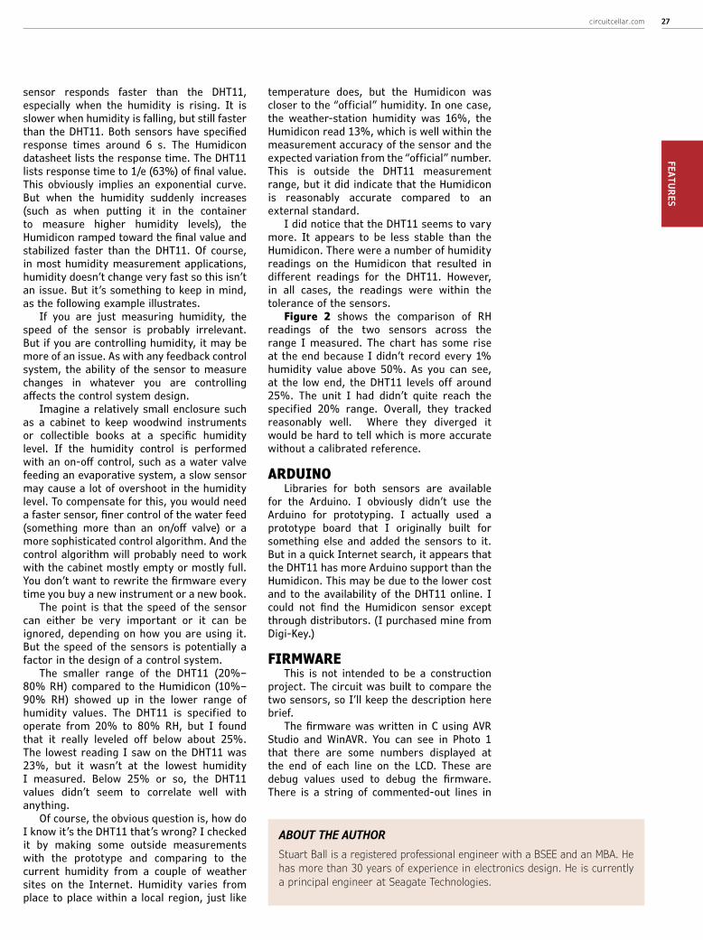
ABOUT THE AUTHORStuart Ball is a registered professional engineer with a BSEE and an MBA. He has more than 30 years of experience in electronics design. He is currently a principal engineer at Seagate Technologies.
CIRCUIT CELLAR • MAY 2015 #29828FE
ATUR
ES
the code that selects one or more values for display. Of course, in a real application, you would probably be using just one sensor, not two, and you would remove both the debug values and the temperature/humidity output for whichever sensor you aren’t using.
Samples are taken every 4 s. The Humidicon is sampled at 2 s, the DHT11 at 4 s, and then the 4-s cycle repeats. Timing is accomplished by allowing the ATmega’s T0 timer to free-run and polling for timer rollover to generate a timebase. No interrupts are used.
ADDING LOGGINGThe purpose of this experiment was to
compare the two sensors, not to create a humidity data-logging system. The prototype doesn’t log the values it records, but adding logging would not be difficult. The ATmega8515 has 512 bytes of EEPROM, which could be used to store up to 512 humidity values. This would allow one sample per minute for an 8-h period, or one every 5 minutes for 42 h. Other microcontrollers have more EEPROM storage, which would allow more samples to be stored. An external SPI or I2C EEPROM memory could be connected to the microcontroller to get even more storage.
The simplest way to log the data is probably to use the serial port on the ATmega8515 (or other microcontroller) to send the temperature data to a laptop. But, if you are logging humidity in a remote location or a sealed enclosure, that might be impractical and you might need to capture it locally. Of course, with a different microcontroller, you may be able to use embedded USB, or you could add a USB module to the ATmega8515.
The easiest way to start logging is to connect a pushbutton switch between one of the unused inputs and ground, and press it to start, and again to stop. The switch can be debounced in the firmware, of course, and it can be pulled high with an external resistor or
the internal resistor on the ATmega I/O pin. Use the serial port on the microcontroller to download the logged data to a PC.
RESULTSThere is a sensor similar to the DHT11
called the DHT21, which has a wider range of measurement. It is specified at 0–100% RH. Honeywell makes a Humidicon HIH 9000 series that has 1.7% accuracy instead of 4%. I did not test either of them, but either of those would be expected to perform better than the units I tested if wider range or better accuracy is needed.
The DHT11 is an inexpensive humidity/temperature sensor suitable for many applications. At the low end of its range, the unit I had did not perform as well as the Honeywell sensor and did not seem to even reach the limit of its specification. However, this could be a problem with the sensor; other individual samples may perform better. Although this was not a laboratory-grade experiment with sophisticated humidity chambers, the simple experiments I did do indicate the differences between the two sensors.
The Humidicon was significantly more expensive than the DHT11, at about $13. I admit that I wanted it to work significantly better than the DHT11, but the performance was comparable within the specified ranges. If I wanted repeatable accuracy for an application that might have to work at low humidity values, I would use the Humidicon. If you don’t expect to read low humidity values, then either would probably work.
Clearly if you need outdoor operation, you would want to use the Humidicon sensor. The DHT11 can only measure down to 0°C, which makes it unsuitable for use outdoors, unless you live near the equator. The Humidicon is not compensated below 5°C, but it will measure temperatures below freezing. I did test the Humidicon below freezing and the humidity reading was within tolerance to the value from an Internet website. So, even though the humidity value is not calibrated below 0°C, it is capable of making readings at lower temperatures.
Either sensor can measure humidity and temperature. But this comparison is instructive in demonstrating the limits of different sensors and how they can impact your design. Making designs interact with the real world involves trade-offs between cost, accuracy, measurement range, and sensor speed, and all of those have to be considered against the intended purpose of the design. Although the example used in this article was not intended to be a sellable product, it does illustrate the trade-offs involved.
circuitcellar.com/ccmaterials
RESOURCEHoneywell, “I2C Communi-cation with the Honeywell HumidIcon Digital Humid-ity/Temperature Sensors,”
009061-2-EN, 2012, http://sensing.honeywell.com/i2c-comms-humidicon-tn-009061-2-en-fi-nal-07jun12.pdf.
SOURCES ATmega8515 microcontroller
Atmel Corp. | www.atmel.com
Humidicon
Honeywell | www.honeywell.com


CIRCUIT CELLAR • MAY 2015 #29830FE
ATUR
ES
I built an Arduino-based monitor to retrieve particulate matter (PM) and wet bulb globe
temperature (WBGT) values from the Internet and display them in an RGB LED matrix. The
values are updated hourly and shown with specific colors that indicate different safety conditions. I use a cloud service for plotting and remotely monitoring the unit.
Atmospheric Particulate Matter Monitor
The Particulate Matter Monitor retrieves particulate matter (PM) information from the Internet and displays it on an LED matrix. When the PM concentration in the air rises above accepted levels, the system presents the values in red. Otherwise, the data is presented in green.
By J. Alejandro Butrón-Guillén (Japan)
PHOTO 1This is PM2.5 data for different places in Fukuoka prefecture, Japan. This information is provided by the Fukuoka Institute of Health and Environmental Sciences. The information for the Wakamatsu ward region is located at the top line, marked with a red rectangle.

circuitcellar.com 31FEATURES
PM & WBGTPM comprises tiny pieces of material
(micrometers) that are suspended in the atmosphere. These particulates are generated from industrial activities and natural phenomena (e.g., volcanoes). Since they can adversely affect human health, they are subject to regulations by industrialized countries as well as the World Health Organization.
In this article, I consider the PM value of 2.5 µm, which is abbreviated as PM2.5. Governments in different countries are measuring the PM2.5 levels and placing this data on the Internet for official and public
use. Photo 1 shows a Japanese webpage with relevant PM2.5 information. The Japanese Ministry of the Environment has established that PM2.5 values up to 35 µg per cubic meter are acceptable. But when values increase to 36 µg per cubic meter or more, the population (especially small children and the elderly) is at risk. This is reflected in the color of the numbers for the different measures.
As a consequence of the Global Warming, now we need to be concerned about the WBGT and take precautionary measures. Here in Japan, the WBGT is of particular interest during the summer months as children participate in sporting event. Photo 2 shows
PHOTO 2The Japanese Ministry of the Environment’s webpage shows the WBGT data over a map of Japan. The color scale at the bottom indicates the following: up to 21 (blue) indicates fairly safe conditions; 25 (green) alters you to be cautious; 28 (yellow) is a warning; 31 (orange) is a severe warning; and more than 31 (red) indicates danger. The units are in degrees Celsius.
PHOTO 3The webpage of the Japanese Ministry of the Environment showing hourly WBGT values for Munakata City (the closest place to Ebitsu). These values are displayed on the PM2.5 and WBGT monitor, which is located at the Ebitsu Primary School.
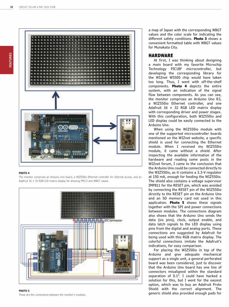
CIRCUIT CELLAR • MAY 2015 #29832FE
ATUR
ES
a map of Japan with the corresponding WBGT values and the color scale for indicating the different safety conditions. Photo 3 shows a convenient formatted table with WBGT values for Munakata City.
HARDWAREAt first, I was thinking about designing
a main board with my favorite Microchip Technology PIC18F microcontroller, but developing the corresponding library for the WIZnet W5500 chip would have taken too long. Thus, I went with off-the-shelf components. Photo 4 depicts the entire system, with an indication of the signal flow between components. As you can see, the monitor comprises an Arduino Uno R3, a WIZ550io Ethernet controller, and one Adafruit 16 × 32 RGB LED matrix display with corresponding driver and power stages. With this configuration, both WIZ550io and LED display could be easily connected to the Arduino Uno.
When using the WIZ550io module with one of the supported microcontroller boards mentioned on the WIZnet website, a specific shield is used for connecting the Ethernet module. When I received my WIZ550io module, it came without a shield. After inspecting the available information of the hardware and reading some posts in the WIZnet forum, I came to the conclusion that the Arduino Uno could be connected directly to the WIZ550io, as it contains a 3.3-V regulator at 150 mA, enough for feeding the WIZ550io. The shield also contains a voltage supervisor IMP811 for the RESET pin, which was avoided by connecting the RESET pin of the WIZ550io directly to the RESET pin on the Arduino Uno and an SD memory card not used in this application. Photo 5 shows these signals together with the SPI and power connections between modules. The connections diagram also shows that the Arduino Uno sends the data (six pins), clock, output enable, and data latch signals to the LED display using pins from the digital and analog ports. These connections are suggested by Adafruit for being used with this RGB matrix display. The colorful connections imitate the Adafruit’s indications, for easy comparison.
For placing the WIZ550io in top of the Arduino and give adequate mechanical support as a single unit, a general perforated board was been considered, just to discover that the Arduino Uno board has one line of connectors misaligned within the standard separation of 0.1″. I could have hacked a solution for this, but I went for the easiest option, which was to buy an Adafruit Proto Shield with the correct alignment. The generic shield also provided enough pads for
PHOTO 4The monitor comprises an Arduino Uno board, a WIZ550io Ethernet controller for Internet access, and an Adafruit 16 × 32 RGB LED matrix display for showing PM2.5 and WBGT values.
PHOTO 5These are the connections between the monitor’s modules.
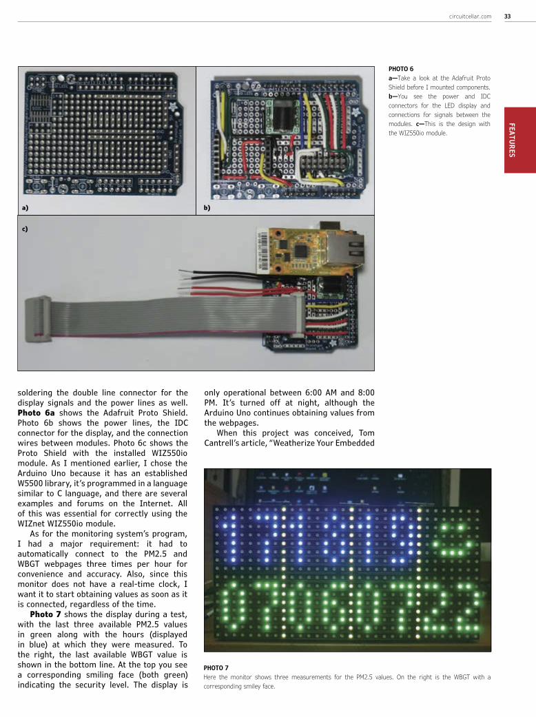
circuitcellar.com 33FEATURES
soldering the double line connector for the display signals and the power lines as well. Photo 6a shows the Adafruit Proto Shield. Photo 6b shows the power lines, the IDC connector for the display, and the connection wires between modules. Photo 6c shows the Proto Shield with the installed WIZ550io module. As I mentioned earlier, I chose the Arduino Uno because it has an established W5500 library, it’s programmed in a language similar to C language, and there are several examples and forums on the Internet. All of this was essential for correctly using the WIZnet WIZ550io module.
As for the monitoring system’s program, I had a major requirement: it had to automatically connect to the PM2.5 and WBGT webpages three times per hour for convenience and accuracy. Also, since this monitor does not have a real-time clock, I want it to start obtaining values as soon as it is connected, regardless of the time.
Photo 7 shows the display during a test, with the last three available PM2.5 values in green along with the hours (displayed in blue) at which they were measured. To the right, the last available WBGT value is shown in the bottom line. At the top you see a corresponding smiling face (both green) indicating the security level. The display is
only operational between 6:00 AM and 8:00 PM. It’s turned off at night, although the Arduino Uno continues obtaining values from the webpages.
When this project was conceived, Tom Cantrell’s article, “Weatherize Your Embedded
PHOTO 7Here the monitor shows three measurements for the PM2.5 values. On the right is the WBGT with a corresponding smiley face.
PHOTO 6a—Take a look at the Adafruit Proto Shield before I mounted components. b—You see the power and IDC connectors for the LED display and connections for signals between the modules. c—This is the design with the WIZ550io module.
a) b)
c)
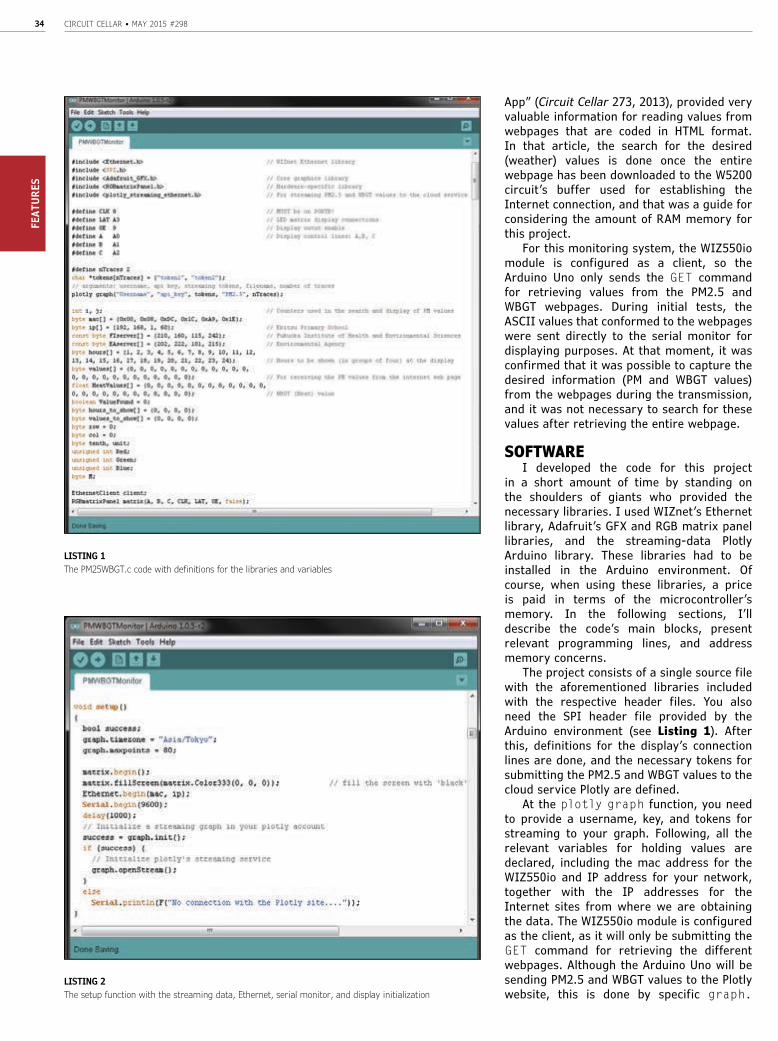
CIRCUIT CELLAR • MAY 2015 #29834FE
ATUR
ES
App” (Circuit Cellar 273, 2013), provided very valuable information for reading values from webpages that are coded in HTML format. In that article, the search for the desired (weather) values is done once the entire webpage has been downloaded to the W5200 circuit’s buffer used for establishing the Internet connection, and that was a guide for considering the amount of RAM memory for this project.
For this monitoring system, the WIZ550io module is configured as a client, so the Arduino Uno only sends the GET command for retrieving values from the PM2.5 and WBGT webpages. During initial tests, the ASCII values that conformed to the webpages were sent directly to the serial monitor for displaying purposes. At that moment, it was confirmed that it was possible to capture the desired information (PM and WBGT values) from the webpages during the transmission, and it was not necessary to search for these values after retrieving the entire webpage.
SOFTWAREI developed the code for this project
in a short amount of time by standing on the shoulders of giants who provided the necessary libraries. I used WIZnet’s Ethernet library, Adafruit’s GFX and RGB matrix panel libraries, and the streaming-data Plotly Arduino library. These libraries had to be installed in the Arduino environment. Of course, when using these libraries, a price is paid in terms of the microcontroller’s memory. In the following sections, I’ll describe the code’s main blocks, present relevant programming lines, and address memory concerns.
The project consists of a single source file with the aforementioned libraries included with the respective header files. You also need the SPI header file provided by the Arduino environment (see Listing 1). After this, definitions for the display’s connection lines are done, and the necessary tokens for submitting the PM2.5 and WBGT values to the cloud service Plotly are defined.
At the plotly graph function, you need to provide a username, key, and tokens for streaming to your graph. Following, all the relevant variables for holding values are declared, including the mac address for the WIZ550io and IP address for your network, together with the IP addresses for the Internet sites from where we are obtaining the data. The WIZ550io module is configured as the client, as it will only be submitting the GET command for retrieving the different webpages. Although the Arduino Uno will be sending PM2.5 and WBGT values to the Plotly website, this is done by specific graph.
LISTING 1The PM25WBGT.c code with definitions for the libraries and variables
LISTING 2The setup function with the streaming data, Ethernet, serial monitor, and display initialization

OPEN
RUGGED
LONG LIFE
ORIGIN
ALUnique embedded solutions add value for our customers
Support every step of the way with open source vision
Embedded systems that are built to endure
We’ve never discontinued a product in 30 years
DESIGN YOUR SOLUTION TODAYCALL 480-837-5200
TS-4900 Computer Module1 GHz i.MX6 with WiFi & Bluetooth
Available w/ TS-TPC-8390Touch Panel Computer
TS-7970: SBC Versionof the TS-4900NEW!
Pricing Starts At
$122Qty 1
Qty 100
$89
1 GHz Single or Quad Core Cortex A9 ARM CPU
-40 ºC to 85 ºC Industrial Temperature Range
4 KLut FPGA, 1x Gigabit Ethernet, 1x PCI Express Bus
Wireless 802.11 b/g/n and Bluetooth 4.0
1x mSD slot, 1x SATA II, 1x USB Host, 1x USB OTG
Up to 2 GB DDR3 RAM and 4 GB eMMC Flash
70x DIO, 4x I2C, 1x I2S, 2x SPI, 2x CAN
Runs Android, QNX, Linux 3.10, Yocto, QT, OpenGL
1x LVDS & 1x RGB Display Port
Coming Soon: Windows Support
Pricing starts at$203
Qty 1Qty 100
$159
TS-7680 Industrial ComputerAC Power, Relays, WiFi and Bluetooth
Guaranteed available until 2025
Easy development w/ Debian and Linux 2.6Boots quickly to your Embedded Application
Low power with 10mW sleep stateBenefits:
-40 to +85C, 100% soldered-on components
454MHz ARM CPU
Up to 256MB RAM
1x USB Host
4x 30 VDC DIO
1x microSD Socket
2GB NAND/eMMC Flash
2x 3A Relays, 2x CAN
6x ADC, 4x DAC
2x 10/100 Ethernet 2x RS-232, 2x RS-485
Features:
Also Available:TS-7670: Like the TS-7680 w/ GPS and Cellular Modem
low cost plasticenclosure available
COMING
SOON!
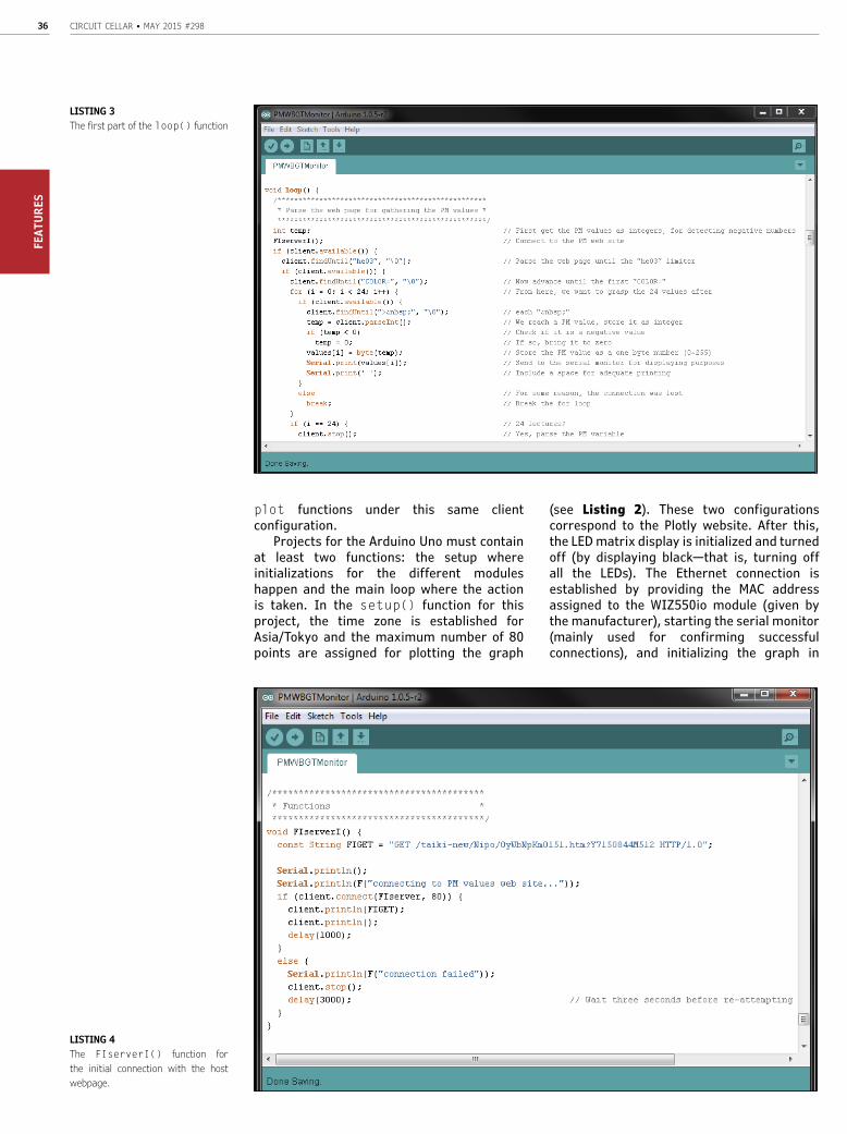
CIRCUIT CELLAR • MAY 2015 #29836FE
ATUR
ES
plot functions under this same client configuration.
Projects for the Arduino Uno must contain at least two functions: the setup where initializations for the different modules happen and the main loop where the action is taken. In the setup() function for this project, the time zone is established for Asia/Tokyo and the maximum number of 80 points are assigned for plotting the graph
(see Listing 2). These two configurations correspond to the Plotly website. After this, the LED matrix display is initialized and turned off (by displaying black—that is, turning off all the LEDs). The Ethernet connection is established by providing the MAC address assigned to the WIZ550io module (given by the manufacturer), starting the serial monitor (mainly used for confirming successful connections), and initializing the graph in
LISTING 3The first part of the loop() function
LISTING 4The FIserverI() function for the initial connection with the host webpage.
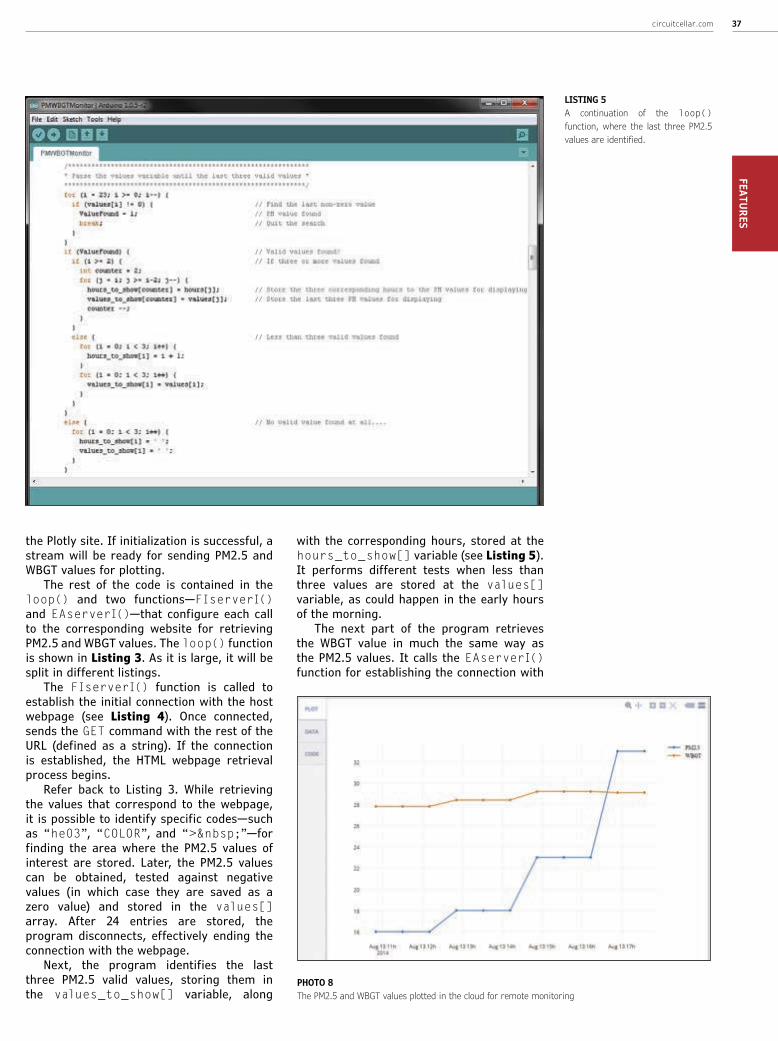
circuitcellar.com 37FEATURES
the Plotly site. If initialization is successful, a stream will be ready for sending PM2.5 and WBGT values for plotting.
The rest of the code is contained in the loop() and two functions—FIserverI() and EAserverI()—that configure each call to the corresponding website for retrieving PM2.5 and WBGT values. The loop() function is shown in Listing 3. As it is large, it will be split in different listings.
The FIserverI() function is called to establish the initial connection with the host webpage (see Listing 4). Once connected, sends the GET command with the rest of the URL (defined as a string). If the connection is established, the HTML webpage retrieval process begins.
Refer back to Listing 3. While retrieving the values that correspond to the webpage, it is possible to identify specific codes—such as “he03”, “COLOR”, and “> ”—for finding the area where the PM2.5 values of interest are stored. Later, the PM2.5 values can be obtained, tested against negative values (in which case they are saved as a zero value) and stored in the values[] array. After 24 entries are stored, the program disconnects, effectively ending the connection with the webpage.
Next, the program identifies the last three PM2.5 valid values, storing them in the values_to_show[] variable, along
with the corresponding hours, stored at the hours_to_show[] variable (see Listing 5). It performs different tests when less than three values are stored at the values[] variable, as could happen in the early hours of the morning.
The next part of the program retrieves the WBGT value in much the same way as the PM2.5 values. It calls the EAserverI() function for establishing the connection with
LISTING 5A continuation of the loop() function, where the last three PM2.5 values are identified.
PHOTO 8The PM2.5 and WBGT values plotted in the cloud for remote monitoring

CIRCUIT CELLAR • MAY 2015 #29838FE
ATUR
ES
PHOTO 9This is the PM2.5 and WBGT monitor operating at the Ebitsu Primary School in Fukuoka, Japan.
the webpage. According to different markers, it identifies the available WBGT values and these are stored at the HeatValues[] variable. After that, the connection is stopped, and only the last WBGT value is selected.
Once the last three PM2.5 and one WBGT values have been obtained, the PM2.5 values are shown with corresponding colors (green or red, according to the critical value) and hours (in blue) on the matrix display. Yellow lines are shown for separating columns and helping in the visualization of the numbers. In a similar fashion, the WBGT value is shown at the display, with corresponding color and face representation according to the safety values. By verifying the hours during which the values were obtained, the monitor operates only between 06:00 and 20:00.
Finally, for sending the PM2.5 and WBGT values to the cloud service for plotting, two calls are made to the graph.plot() function, with corresponding values and tokens that were defined previously. Photo 8 shows a graph from the Plotly site. You can also see the updated graph at https://plot.ly/~Alex_BG/1. Depending on the month of the year, the WBGT value will or won’t be shown because as the Environment Ministry only posts the data from May to October.
As I already mentioned, by using the different libraries, RAM becomes scarce. To compile the program, the strings used at the serial communication were enclosed with the F() macro for keeping them at program memory. But what really saved the day was the reduction of the 64-byte serial receive buffer to 16 bytes. The definition for this buffer is located in the HardwareSerial.cpp file in the Arduino install directory.
FIELD TESTI placed the PM2.5 and WBGT monitor
modules in a preassembled wood case that matched the size of the display. I added hinges to the top cover so I have easy access to the Arduino Uno. I also inserted holes for the power and Ethernet cables.
I tested the PM2.5 and WBGT monitor at the Ebitsu Primary School in Fukuoka, Japan. I placed it in the administrative office so anyone could see it.
Initially, I had the monitor showing only the PM2.5 values. But at the request of the school nurse, I added the WBGT value. Photo 9 shows the PM2.5 and WBGT monitor in operation.
After few days of testing, I received positive feedback. It was easier for users to glance at the monitor than having to constantly check the PM2.5 and WBGT values on the Internet.
circuitcellar.com/ccmaterials
RESOURCEST. Cantrell, “Weatherize Your Embedded App”, Circuit Cel-lar, April 2013.
Fukuoka Institute of Health and Environmental Scienc-es, PM2.5 Values, www.fihes.pref.fukuoka.jp/taiki-new/Nipo/OyWbNpKm0151.ht-m?Y7850841GR12.
Japanese Ministry of the Environment, WBGT Values, www.wbgt.env.go.jp/day_list.php?re-gion=10&prefecture=82&point=82046. World Health Organization, “Ambient (Outdoor) Air Quality and Health,” Factsheet 313, 2014, www.who.int/mediacentre/factsheets/fs313/en/. SOURCESMedium 16 × 32 RGB LED matrix panel
Adafruit Industries | www.adafruit.com
Arduino Uno R3
Arduino | www.arduino.cc
WIZ550io Ethernet controller
WIZnet | www.wiznet.co.kr
ABOUT THE AUTHORJ. Alejandro Butrón-Guillén ([email protected]) is an electronics engineer interested in embedded systems, robotics and dig-ital signal processing.

For more information visit: circuitcellar.newhavendisplay.com Contact us at: 847-844-8795
NEWHAVEN DISPLAY INTERNATIONAL
•Vivid•Organic•Affordable
• Only 5 mm thin
• 2x16, 2x20, and 4x20 character sizes
• Yellow, Blue, Red or Green colors
• Response time: 10 microseconds
• SPI, I2C & Parallel interfaces
• Operating temp: (-40°C ~ +85°C)
• Storage temp: (-40°C ~ +90°C)
• US2066 Built-in controller
• Contrast ratio: 10,000:1
• Viewing angle: >160°
OLEDs• Low power 2.4 ~ 3.6VDD
• Double height characters
• 3 built-in font tables
• Built-in required logic
• Built-in screen saver
Slim
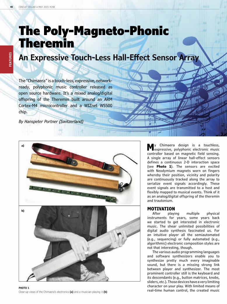
CIRCUIT CELLAR • MAY 2015 #29840FE
ATUR
ES
My Chimaera design is a touchless, expressive, polyphonic electronic music
controller based on magnetic field sensing. A single array of linear hall-effect sensors defines a continuous 2-D interaction space (see Photo 1). The sensors are excited with Neodymium magnets worn on fingers whereby their position, vicinity and polarity are continuously tracked along the array to serialize event signals accordingly. These event signals are transmitted to a host and flexibly mapped to musical events. Think of it as an analog/digital offspring of the theremin and trautonium.
MOTIVATIONAfter playing multiple physical
instruments for years, some years back we started to get interested in electronic music. The shear unlimited possibilities of digital audio synthesis fascinated us. For an intuitive player all the semiautomated (e.g., sequencing) or fully automated (e.g., algorithmic) electronic composition styles are not that interesting, though.
The various audio programming languages and software synthesizers enable you to synthesize pretty much every imaginable sound, but there is a missing strong link between player and synthesizer. The most prominent controller still is the keyboard and its descendants (e.g., button matrices, knobs, sliders, etc.). Those devices have a very limiting character on your play. With limited means of real-time human control, the created music
The Poly-Magneto-Phonic ThereminAn Expressive Touch-Less Hall-Effect Sensor Array
The “Chimaera” is a touch-less, expressive, network-ready, polyphonic music controller released as open source hardware. It’s a mixed analog/digital offspring of the Theremin built around an ARM Cortex-M4 microcontroller and a WIZnet W5500 chip.
By Hanspeter Portner (Switzerland)
PHOTO 1Close-up views of the Chimaera’s electronics (a) and a musician playing it (b)
a)
b)
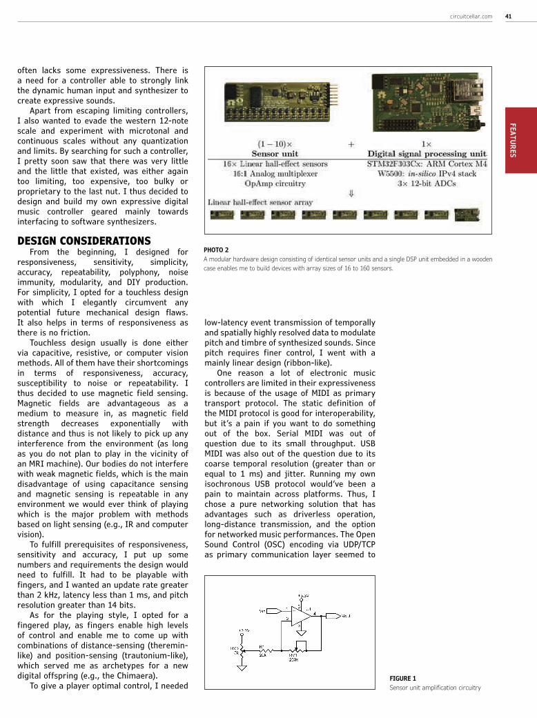
circuitcellar.com 41FEATURES
often lacks some expressiveness. There is a need for a controller able to strongly link the dynamic human input and synthesizer to create expressive sounds.
Apart from escaping limiting controllers, I also wanted to evade the western 12-note scale and experiment with microtonal and continuous scales without any quantization and limits. By searching for such a controller, I pretty soon saw that there was very little and the little that existed, was either again too limiting, too expensive, too bulky or proprietary to the last nut. I thus decided to design and build my own expressive digital music controller geared mainly towards interfacing to software synthesizers.
DESIGN CONSIDERATIONSFrom the beginning, I designed for
responsiveness, sensitivity, simplicity, accuracy, repeatability, polyphony, noise immunity, modularity, and DIY production. For simplicity, I opted for a touchless design with which I elegantly circumvent any potential future mechanical design flaws. It also helps in terms of responsiveness as there is no friction.
Touchless design usually is done either via capacitive, resistive, or computer vision methods. All of them have their shortcomings in terms of responsiveness, accuracy, susceptibility to noise or repeatability. I thus decided to use magnetic field sensing. Magnetic fields are advantageous as a medium to measure in, as magnetic field strength decreases exponentially with distance and thus is not likely to pick up any interference from the environment (as long as you do not plan to play in the vicinity of an MRI machine). Our bodies do not interfere with weak magnetic fields, which is the main disadvantage of using capacitance sensing and magnetic sensing is repeatable in any environment we would ever think of playing which is the major problem with methods based on light sensing (e.g., IR and computer vision).
To fulfill prerequisites of responsiveness, sensitivity and accuracy, I put up some numbers and requirements the design would need to fulfill. It had to be playable with fingers, and I wanted an update rate greater than 2 kHz, latency less than 1 ms, and pitch resolution greater than 14 bits.
As for the playing style, I opted for a fingered play, as fingers enable high levels of control and enable me to come up with combinations of distance-sensing (theremin-like) and position-sensing (trautonium-like), which served me as archetypes for a new digital offspring (e.g., the Chimaera).
To give a player optimal control, I needed
low-latency event transmission of temporally and spatially highly resolved data to modulate pitch and timbre of synthesized sounds. Since pitch requires finer control, I went with a mainly linear design (ribbon-like).
One reason a lot of electronic music controllers are limited in their expressiveness is because of the usage of MIDI as primary transport protocol. The static definition of the MIDI protocol is good for interoperability, but it’s a pain if you want to do something out of the box. Serial MIDI was out of question due to its small throughput. USB MIDI was also out of the question due to its coarse temporal resolution (greater than or equal to 1 ms) and jitter. Running my own isochronous USB protocol would’ve been a pain to maintain across platforms. Thus, I chose a pure networking solution that has advantages such as driverless operation, long-distance transmission, and the option for networked music performances. The Open Sound Control (OSC) encoding via UDP/TCP as primary communication layer seemed to
PHOTO 2A modular hardware design consisting of identical sensor units and a single DSP unit embedded in a wooden case enables me to build devices with array sizes of 16 to 160 sensors.
FIGURE 1 Sensor unit amplification circuitry

CIRCUIT CELLAR • MAY 2015 #29842FE
ATUR
ES
be the right choice for these highly resolved events.
HARDWAREThe Chimaera’s hardware consists of a
sensor and digital signal processing (DSP) unit, some cabling, and an enclosure (see Photo 2). Multiple sensor units are daisy-chained to form the sensor array and connected to a single DSP unit. A modular design with multiple identical PCBs is advantageous for DIY production as it is cheaper to order multiple identical small PCBs than one large one. It also helps to distribute heat along the sensor array with a per unit voltage regulator as the sensors draw around 10 mA each.
The sensor unit is a mostly analog PCB. It embeds 16 linear Hall effect sensors in a straight line 5-mm apart. The analog sensor outputs are connected to a 16:1 analog
multiplexer (74HC4067), which is switched via four digital lines by the DSP unit. The analog signal runs through a simple shifting amplification circuitry after the multiplexer (see Figure 1). An initial version was based on 5-V through-hole sensors (the A1301 from Allegro Microsystems). It was really tedious work to solder and it demanded a two-voltage design—that is, 5 V for the sensor units and 3.3 V for the DSP unit. I then changed the design to single-sided surface mount parts to simplify (and potentially automate) construction. In a second step of redesign, I switched to a newly released and less costly 3.3-V sensor (A1304). To create an equally responding continuous sensor array all units need comparable tuning at their trim potentiometers RV1 and RV3 (see Figure 1). RV3 acts as a voltage divider to set reference voltage VREF from VEE(GND) to VCC (3.3 V). Most linear Hall effect sensors respond
Sensor dump
Areas of interest
Sensor value normalization
Blob detection
Vicinity estimation
Polynomial blob interpolation
Blob tracking over space and time
Event data generation(position Xi, vicinity Yi, polarity Pi, group Gi)
Sensor calibratiion
Magnet calibration
FIGURE 2The firmware generates ON, OFF, and SET events per blob out of a raw sensor dump. The vicinity-magnetic field relationship of permanent magnets and differences in sensor sensitivity are taken into account with a two-step calibration.
1.0
0.8
0.6
0.4
0.2
0
xn (Rel. position)
0.21 0.22 0.23 0.24
1.0
0.8
0.6
0.4
0.2
0
Bn (Rel. magnetic field)
0.0 0.40.2 0.6 0.8 1.0
yn(Rel. vicinity)
yn(Rel. vicinity)
FIGURE 3a—Example distance magnetic field relationship (points) and its least-squares fit (line). b—Cubic interpolation of position xn and vicinity yn over four normalized adjacent sensor values with Catmull-Rom splines.
a) b)

Experience extraordinary training
for embedded systems professionals
at ESC Conference Series 2015!
The Embedded Systems Conference (ESC) is the industry’s largest, most comprehensive technical conference for embedded systems
professionals in the U.S. ESC is excited to announce an expanded 2015 USA Conference Series, taking place in Boston (May 6-7), Silicon
Valley (July 20-22), and Minneapolis (November 4-5).
ESC’s first stop in 2015 is Boston, MA, known for its good mix of hi-tech, biotech/life sciences, medical device, and military defense companies. It’s also home to the #1
engineering university in the world - MIT.
Come join us at the Boston Convention Center and check out some of
our sponsors for the event:
Rohde & Schwarz | Green Hills Software, Inc | AdaCore| Altium, Inc.
AMP Display | Azul Systems, Inc. | Convergence Promotions | IAR Systems AB
Ironwood Electronics | MathWorks | Rigol Technologies | SmartBear Software
Symmetry Electronics | Technologic Systems | Teledyne LeCroy
Toradex | Total Phase | Vision Components GmbH | WolfSSL | Lauterbach, Inc.
Phoenix Contract Software | Security Innovation | Code
e-con Systems India Pvt. Ltd | Express Logic | XJTAG
Register today at www.embeddedconf.com/boston and get 15% off a Conference Pass when using a promo code CircuitCellar15Bos, offer expires May 1, 2015.
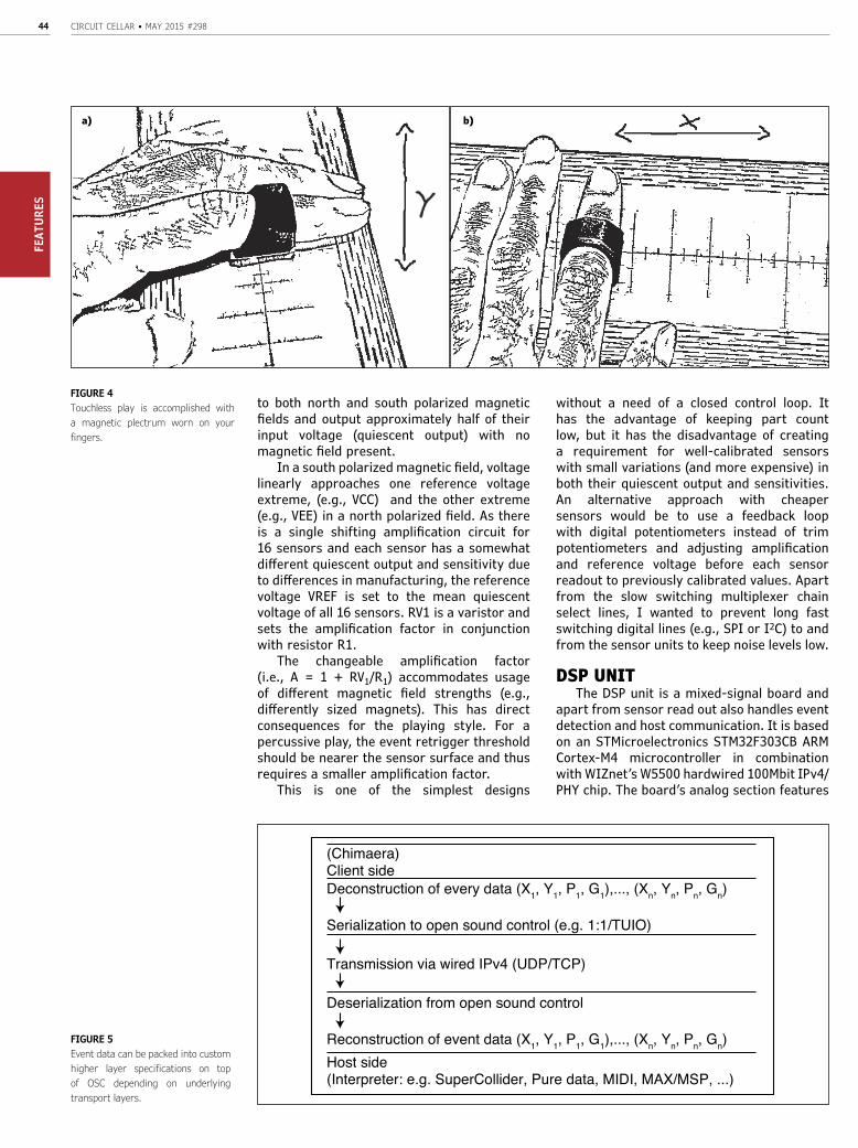
CIRCUIT CELLAR • MAY 2015 #29844FE
ATUR
ES
to both north and south polarized magnetic fields and output approximately half of their input voltage (quiescent output) with no magnetic field present.
In a south polarized magnetic field, voltage linearly approaches one reference voltage extreme, (e.g., VCC) and the other extreme (e.g., VEE) in a north polarized field. As there is a single shifting amplification circuit for 16 sensors and each sensor has a somewhat different quiescent output and sensitivity due to differences in manufacturing, the reference voltage VREF is set to the mean quiescent voltage of all 16 sensors. RV1 is a varistor and sets the amplification factor in conjunction with resistor R1.
The changeable amplification factor (i.e., A = 1 + RV1/R1) accommodates usage of different magnetic field strengths (e.g., differently sized magnets). This has direct consequences for the playing style. For a percussive play, the event retrigger threshold should be nearer the sensor surface and thus requires a smaller amplification factor.
This is one of the simplest designs
without a need of a closed control loop. It has the advantage of keeping part count low, but it has the disadvantage of creating a requirement for well-calibrated sensors with small variations (and more expensive) in both their quiescent output and sensitivities. An alternative approach with cheaper sensors would be to use a feedback loop with digital potentiometers instead of trim potentiometers and adjusting amplification and reference voltage before each sensor readout to previously calibrated values. Apart from the slow switching multiplexer chain select lines, I wanted to prevent long fast switching digital lines (e.g., SPI or I2C) to and from the sensor units to keep noise levels low.
DSP UNITThe DSP unit is a mixed-signal board and
apart from sensor read out also handles event detection and host communication. It is based on an STMicroelectronics STM32F303CB ARM Cortex-M4 microcontroller in combination with WIZnet’s W5500 hardwired 100Mbit IPv4/PHY chip. The board’s analog section features
FIGURE 4Touchless play is accomplished with a magnetic plectrum worn on your fingers.
(Chimaera)Client sideDeconstruction of every data (X1, Y1, P1, G1),..., (Xn, Yn, Pn, Gn)
Serialization to open sound control (e.g. 1:1/TUIO)
Transmission via wired IPv4 (UDP/TCP)
Deserialization from open sound control
Reconstruction of event data (X1, Y1, P1, G1),..., (Xn, Yn, Pn, Gn) Host side(Interpreter: e.g. SuperCollider, Pure data, MIDI, MAX/MSP, ...)
FIGURE 5 Event data can be packed into custom higher layer specifications on top of OSC depending on underlying transport layers.
a) b)

From home control systems to
animatronic toys to unmanned
rovers, it’s an exciting time to
be a roboticist. Advanced Control Robotics
simplifies the theory and best practices of
advanced robot technologies, making
it ideal reading for beginners and experts
alike. You’ll gain superior knowledge of
embedded design theory by way of
handy code samples, essential schematics,
and valuable design tips.
With this book, you’ll learn about:
Get it today at ccwebshop.com.
When it comes to robotics,the future is now!
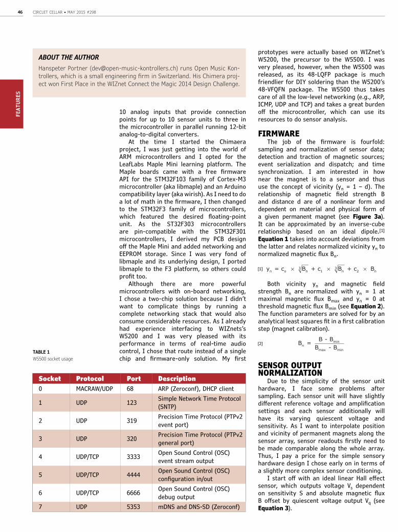
CIRCUIT CELLAR • MAY 2015 #29846FE
ATUR
ES
10 analog inputs that provide connection points for up to 10 sensor units to three in the microcontroller in parallel running 12-bit analog-to-digital converters.
At the time I started the Chimaera project, I was just getting into the world of ARM microcontrollers and I opted for the LeafLabs Maple Mini learning platform. The Maple boards came with a free firmware API for the STM32F103 family of Cortex-M3 microcontroller (aka libmaple) and an Arduino compatibility layer (aka wirish). As I need to do a lot of math in the firmware, I then changed to the STM32F3 family of microcontrollers, which featured the desired floating-point unit. As the ST32F303 microcontrollers are pin-compatible with the STM32F301 microcontrollers, I derived my PCB design off the Maple Mini and added networking and EEPROM storage. Since I was very fond of libmaple and its underlying design, I ported libmaple to the F3 platform, so others could profit too.
Although there are more powerful microcontrollers with on-board networking, I chose a two-chip solution because I didn’t want to complicate things by running a complete networking stack that would also consume considerable resources. As I already had experience interfacing to WIZnets’s W5200 and I was very pleased with its performance in terms of real-time audio control, I chose that route instead of a single chip and firmware-only solution. My first
prototypes were actually based on WIZnet’s W5200, the precursor to the W5500. I was very pleased, however, when the W5500 was released, as its 48-LQFP package is much friendlier for DIY soldering than the W5200’s 48-VFQFN package. The W5500 thus takes care of all the low-level networking (e.g., ARP, ICMP, UDP and TCP) and takes a great burden off the microcontroller, which can use its resources to do sensor analysis.
FIRMWAREThe job of the firmware is fourfold:
sampling and normalization of sensor data; detection and traction of magnetic sources; event serialization and dispatch; and time synchronization. I am interested in how near the magnet is to a sensor and thus use the concept of vicinity (yn = 1 – d). The relationship of magnetic field strength B and distance d are of a nonlinear form and dependent on material and physical form of a given permanent magnet (see Figure 3a). It can be approximated by an inverse-cube relationship based on an ideal dipole.[1]
Equation 1 takes into account deviations from the latter and relates normalized vicinity yn to normalized magnetic flux Bn.
y = c + c + c Bn o 1 2 n× × ×B Bn n3 3
Both vicinity yn and magnetic field strength Bn are normalized with yn = 1 at maximal magnetic flux Bmax and yn = 0 at threshold magnetic flux Bmin (see Equation 2). The function parameters are solved for by an analytical least squares fit in a first calibration step (magnet calibration).
B = - B - Bn
min
min
BBmax
SENSOR OUTPUT NORMALIZATION
Due to the simplicity of the sensor unit hardware, I face some problems after sampling. Each sensor unit will have slightly different reference voltage and amplification settings and each sensor additionally will have its varying quiescent voltage and sensitivity. As I want to interpolate position and vicinity of permanent magnets along the sensor array, sensor readouts firstly need to be made comparable along the whole array. Thus, I pay a price for the simple sensory hardware design I chose early on in terms of a slightly more complex sensor conditioning.
I start off with an ideal linear Hall effect sensor, which outputs voltage Vs dependent on sensitivity S and absolute magnetic flux B offset by quiescent voltage output Vq (see Equation 3).
TABLE 1 W5500 socket usage
Socket Protocol Port Description0 MACRAW/UDP 68 ARP (Zeroconf), DHCP client
1 UDP 123 Simple Network Time Protocol (SNTP)
2 UDP 319 Precision Time Protocol (PTPv2 event port)
3 UDP 320 Precision Time Protocol (PTPv2 general port)
4 UDP/TCP 3333 Open Sound Control (OSC) event stream output
5 UDP/TCP 4444 Open Sound Control (OSC) configuration in/out
6 UDP/TCP 6666 Open Sound Control (OSC) debug output
7 UDP 5353 mDNS and DNS-SD (Zeroconf)
ABOUT THE AUTHORHanspeter Portner ([email protected]) runs Open Music Kon-trollers, which is a small engineering firm in Switzerland. His Chimera proj-ect won First Place in the WIZnet Connect the Magic 2014 Design Challenge.
[1]
[2]
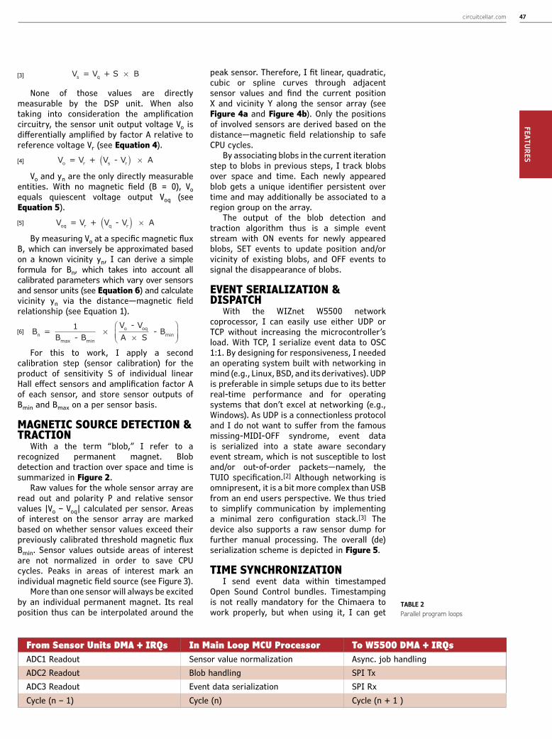
circuitcellar.com 47FEATURES
Vs = V + S Bq ×
None of those values are directly measurable by the DSP unit. When also taking into consideration the amplification circuitry, the sensor unit output voltage Vo is differentially amplified by factor A relative to reference voltage Vr (see Equation 4).
Vo r s r = V + V - V A( ) ×
Vo and yn are the only directly measurable entities. With no magnetic field (B = 0), Vo equals quiescent voltage output Voq (see Equation 5).
Voq r q r = V + V - V A( ) ×
By measuring Vo at a specific magnetic flux B, which can inversely be approximated based on a known vicinity yn, I can derive a simple formula for Bn, which takes into account all calibrated parameters which vary over sensors and sensor units (see Equation 6) and calculate vicinity yn via the distance—magnetic field relationship (see Equation 1).
B = - B
- V S
- Bnmin
oqmin
1B
VA
o
max
××
⎛⎝⎜
⎞⎠⎟
For this to work, I apply a second calibration step (sensor calibration) for the product of sensitivity S of individual linear Hall effect sensors and amplification factor A of each sensor, and store sensor outputs of Bmin and Bmax on a per sensor basis.
MAGNETIC SOURCE DETECTION & TRACTION
With a the term “blob,” I refer to a recognized permanent magnet. Blob detection and traction over space and time is summarized in Figure 2.
Raw values for the whole sensor array are read out and polarity P and relative sensor values |Vo – Voq| calculated per sensor. Areas of interest on the sensor array are marked based on whether sensor values exceed their previously calibrated threshold magnetic flux Bmin. Sensor values outside areas of interest are not normalized in order to save CPU cycles. Peaks in areas of interest mark an individual magnetic field source (see Figure 3).
More than one sensor will always be excited by an individual permanent magnet. Its real position thus can be interpolated around the
peak sensor. Therefore, I fit linear, quadratic, cubic or spline curves through adjacent sensor values and find the current position X and vicinity Y along the sensor array (see Figure 4a and Figure 4b). Only the positions of involved sensors are derived based on the distance—magnetic field relationship to safe CPU cycles.
By associating blobs in the current iteration step to blobs in previous steps, I track blobs over space and time. Each newly appeared blob gets a unique identifier persistent over time and may additionally be associated to a region group on the array.
The output of the blob detection and traction algorithm thus is a simple event stream with ON events for newly appeared blobs, SET events to update position and/or vicinity of existing blobs, and OFF events to signal the disappearance of blobs.
EVENT SERIALIZATION & DISPATCH
With the WIZnet W5500 network coprocessor, I can easily use either UDP or TCP without increasing the microcontroller’s load. With TCP, I serialize event data to OSC 1:1. By designing for responsiveness, I needed an operating system built with networking in mind (e.g., Linux, BSD, and its derivatives). UDP is preferable in simple setups due to its better real-time performance and for operating systems that don’t excel at networking (e.g., Windows). As UDP is a connectionless protocol and I do not want to suffer from the famous missing-MIDI-OFF syndrome, event data is serialized into a state aware secondary event stream, which is not susceptible to lost and/or out-of-order packets—namely, the TUIO specification.[2] Although networking is omnipresent, it is a bit more complex than USB from an end users perspective. We thus tried to simplify communication by implementing a minimal zero configuration stack.[3] The device also supports a raw sensor dump for further manual processing. The overall (de)serialization scheme is depicted in Figure 5.
TIME SYNCHRONIZATIONI send event data within timestamped
Open Sound Control bundles. Timestamping is not really mandatory for the Chimaera to work properly, but when using it, I can get
TABLE 2Parallel program loops
From Sensor Units DMA + IRQs In Main Loop MCU Processor To W5500 DMA + IRQsADC1 Readout Sensor value normalization Async. job handlingADC2 Readout Blob handling SPI TxADC3 Readout Event data serialization SPI RxCycle (n – 1) Cycle (n) Cycle (n + 1 )
[3]
[4]
[5]
[6]

CIRCUIT CELLAR • MAY 2015 #29848FE
ATUR
ES
rid of network jitter altogether and also derive accurate velocity and acceleration signals apart from only positional ones. The firmware thus comes with an interrupt based implementation of the precision time protocol (PTPv2), whereby I have only found host implementations of the latter for UNICES.[4] For the hosts that cannot run a PTPv2 server, there is a fall back to the simplified network time protocol (SNTPv4) or a run mode without any timestamping altogether.[5]
IMPLEMENTATION DETAILSI use all eight available sockets on the
W5500 (see Table 1). On socket 0, I run a minimal DHCP client implementation and manage ARP probes and announcements
needed for both the Zeroconf and DHCP specifications. On socket 1, I run a SNTPv4 client for low resolution time synchronization. On sockets 2 and 3, I run a PTPv2 client for high-resolution time synchronization. Sockets 4 and 5 are the main OSC communication channels to and from the device. Socket 6 is a debug port and socket 7 finally completes my minimal Zeroconf stack with implementations of mDNS and DNS-SD.
The driver for the W5500 SPI is implemented asynchronously with a minimal need of microcontroller processing with all communication between the microcontroller and W5500 being handled through DMA controllers. On the microcontroller side, an arbitrary array of read access and/or write access jobs can be defined in the main loop and handed over to the driver. The latter handles each individual job in sequence by configuring the DMA and SPI controllers accordingly. After a job has been processed, a DMA interrupt is issued and the next job is prepared until all jobs have been processed.
Like that, while the driver is sending and/or receiving data to/from the W5500 chip, the microcontroller can already process the previously sampled data and/or prepare the next data to send. I thus reach 22 Mbps of raw UDP/TCP data throughput with the microcontroller and its SPI1 peripheral running at 72 MHz and 36 MHz, respectively.
Apart from the W5500 driver running in parallel to the main program loop, sensor readout is running in parallel via DMA controllers. If I thus would follow a single sensor value through time from its point of sampling to network dispatch of the derived event data, it would thus go through three program loop cycles each corresponding to one of the three parallel program loops (see Table 2).
TOUCHLESS CONTROLWith its touchless control (no friction),
high update rates (2 to 4 kHz), its quasi-continuous spatial resolution, and its low-latency response (less than 1 ms), the Chimaera can react instantaneously to most subtle inputs and allows for a highly dynamic and expressive play. Its open source design additionally gives the user all possibilities to further tune hardware and firmware to his or her needs. The Chimaera is a responsive network device thanks to a hard-wired network coprocessor and configured with and communicated by Open Sound Control. This makes it driver-less and straightforward to integrate into any contemporary setup. By freely combining the polyphonic event signals, you can generate augmented, multidimensional musical mappings for the creation of expressive sounds.
circuitcellar.com/ccmaterials
REFERENCES[1] E. Ramsden, Hall-Effect Sensors: Theory and Applica-tion, Newnes, 2011.
[2] M. Kaltenbrunner, T. Bovermann, R. Bencina, and E. Costanza, “TUIO — A Pro-tocol for Table Based Tangible User Interfaces,” in Pro-ceedings of the Workshop on Gesture in Human-Computer Interaction and Simulation, Vannes, 2005.
[3] D. H. Steinberg and S. Cheshire, Zero Configuration Networking: The Definitive Guide, O’Reilly, 2010.
[4] IEEE Std 1588-2008, IEEE Standard for a Precision Clock Synchronization Protocol for Networked Measurement and Control Systems, 2008.
[5] D. L. Mills, “Simple Net-work Time Protocol (SNTP) Version 4 for IPv4, IPv6 and OSI,” Internet Society, 2006, http://tools.ietf.org/html/rfc4330.
RESOURCESE. Catmull and R. Rom, “A Class of Local In-terpolating Splines,” Computer Aided Geometric Design, 1974.
L. Haken, E. Tellman, and P. Wolfe, “An Indis-crete Music Keyboard,” Computer Music Journal, 1998.
J. Paradiso, “Electronic Music: New Ways to Play,” IEEE Spectrum, 1997.
H. Portner, “Chimaera - The Poly-Magneto-Pho-nic Theremin—An Expressive Touch-Less Hall-Effect Sensor Array,” in B. Caramiaux, K. Tahiroglu, R. Fiebrink, and A. Tanaka (eds), Proceedings of the International Conference on New Interfaces for Musical Expression, London, UK, 2014.
O. Sala, “Experimentelle Und Theoretische Grundlagen Des Trautoniums,” Frequenz, 1949.
L. Theremin, “Method Of and Apparatus for the Generation of Sounds,” Patent US1661058 A, 1928.
M. Wright, “Open Sound Control: An Enabling Technology for Musical Networking,” Organised Sound, Vol. 10, Issue 3, 12005.
SOURCESMaple Mini PCBLeaflabs | www.leaflabs.com
STM32F303CB MicrocontrollerSTMicroelectronics | www.st.com
W5500 ChipWIZnet | www.wiznet.co.kr

3Days 18
60+
5,000+100+26+
Hours of Education
9Tracks
Technical Sessions
Speakers
Hours of Networking
Attendees
Sensing Technologies Driving Tomorrow’s Solutions
www.sensorsexpo.com Interested in becoming an exhibitor or sponsoring this year’s event? email us at [email protected]
Discount is off currently published rates. Cannot be combined with other offers or applied to previous registrations.
June 9-11, 2015Long Beach Convention Center • California
Register Today atwith code CC50
for special discount and take advantage of the lowest rate for 2015!
www.sensorsexpo.com
Embedded Systems
Energy Harvesting for Wireless Applications
IoT: Internet of Things
MEMS
Measurement & Detection
Optical Sensing & Detection
Sensors @ Work
Wearables
Wireless
Tracks & Topics Include:
New
New
New
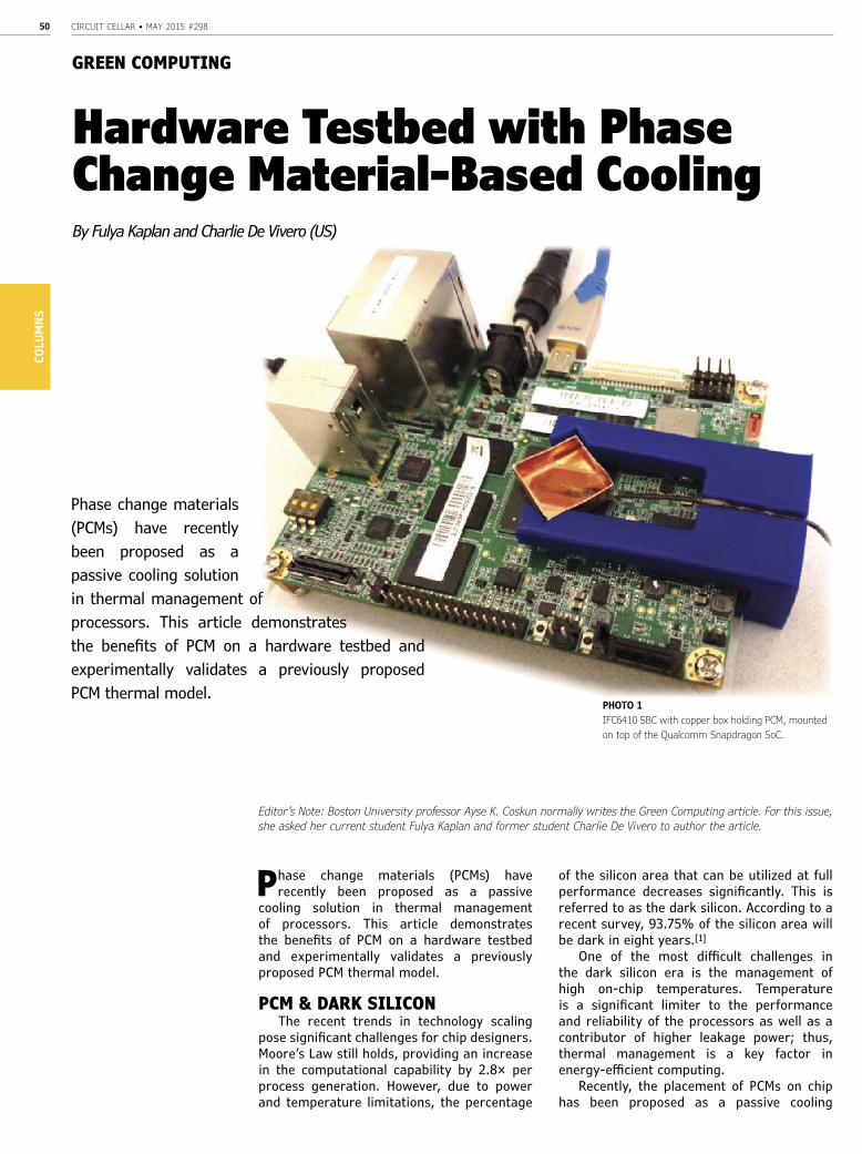
CIRCUIT CELLAR • MAY 2015 #29850CO
LUM
NS
GREEN COMPUTING
Phase change materials (PCMs) have recently been proposed as a passive
cooling solution in thermal management of processors. This article demonstrates the benefits of PCM on a hardware testbed and experimentally validates a previously proposed PCM thermal model.
PCM & DARK SILICON The recent trends in technology scaling
pose significant challenges for chip designers. Moore’s Law still holds, providing an increase in the computational capability by 2.8× per process generation. However, due to power and temperature limitations, the percentage
of the silicon area that can be utilized at full performance decreases significantly. This is referred to as the dark silicon. According to a recent survey, 93.75% of the silicon area will be dark in eight years.[1]
One of the most difficult challenges in the dark silicon era is the management of high on-chip temperatures. Temperature is a significant limiter to the performance and reliability of the processors as well as a contributor of higher leakage power; thus, thermal management is a key factor in energy-efficient computing.
Recently, the placement of PCMs on chip has been proposed as a passive cooling
Hardware Testbed with Phase Change Material-Based Cooling
Phase change materials (PCMs) have recently been proposed as a passive cooling solution in thermal management of processors. This article demonstrates the benefits of PCM on a hardware testbed and experimentally validates a previously proposed PCM thermal model.
By Fulya Kaplan and Charlie De Vivero (US)
PHOTO 1IFC6410 SBC with copper box holding PCM, mounted on top of the Qualcomm Snapdragon SoC.
Editor’s Note: Boston University professor Ayse K. Coskun normally writes the Green Computing article. For this issue, she asked her current student Fulya Kaplan and former student Charlie De Vivero to author the article.
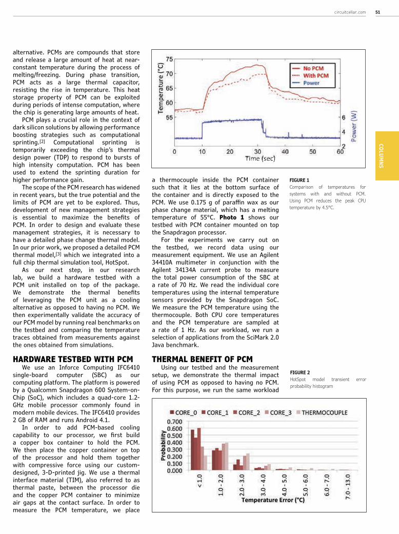
circuitcellar.com 51COLUM
NS
alternative. PCMs are compounds that store and release a large amount of heat at near-constant temperature during the process of melting/freezing. During phase transition, PCM acts as a large thermal capacitor, resisting the rise in temperature. This heat storage property of PCM can be exploited during periods of intense computation, where the chip is generating large amounts of heat.
PCM plays a crucial role in the context of dark silicon solutions by allowing performance boosting strategies such as computational sprinting.[2] Computational sprinting is temporarily exceeding the chip’s thermal design power (TDP) to respond to bursts of high intensity computation. PCM has been used to extend the sprinting duration for higher performance gain.
The scope of the PCM research has widened in recent years, but the true potential and the limits of PCM are yet to be explored. Thus, development of new management strategies is essential to maximize the benefits of PCM. In order to design and evaluate these management strategies, it is necessary to have a detailed phase change thermal model. In our prior work, we proposed a detailed PCM thermal model,[3] which we integrated into a full chip thermal simulation tool, HotSpot.
As our next step, in our research lab, we build a hardware testbed with a PCM unit installed on top of the package. We demonstrate the thermal benefits of leveraging the PCM unit as a cooling alternative as opposed to having no PCM. We then experimentally validate the accuracy of our PCM model by running real benchmarks on the testbed and comparing the temperature traces obtained from measurements against the ones obtained from simulations.
HARDWARE TESTBED WITH PCMWe use an Inforce Computing IFC6410
single-board computer (SBC) as our computing platform. The platform is powered by a Qualcomm Snapdragon 600 System-on-Chip (SoC), which includes a quad-core 1.2-GHz mobile processor commonly found in modern mobile devices. The IFC6410 provides 2 GB of RAM and runs Android 4.1.
In order to add PCM-based cooling capability to our processor, we first build a copper box container to hold the PCM. We then place the copper container on top of the processor and hold them together with compressive force using our custom-designed, 3-D-printed jig. We use a thermal interface material (TIM), also referred to as thermal paste, between the processor die and the copper PCM container to minimize air gaps at the contact surface. In order to measure the PCM temperature, we place
a thermocouple inside the PCM container such that it lies at the bottom surface of the container and is directly exposed to the PCM. We use 0.175 g of paraffin wax as our phase change material, which has a melting temperature of 55°C. Photo 1 shows our testbed with PCM container mounted on top the Snapdragon processor.
For the experiments we carry out on the testbed, we record data using our measurement equipment. We use an Agilent 34410A multimeter in conjunction with the Agilent 34134A current probe to measure the total power consumption of the SBC at a rate of 70 Hz. We read the individual core temperatures using the internal temperature sensors provided by the Snapdragon SoC. We measure the PCM temperature using the thermocouple. Both CPU core temperatures and the PCM temperature are sampled at a rate of 1 Hz. As our workload, we run a selection of applications from the SciMark 2.0 Java benchmark.
THERMAL BENEFIT OF PCMUsing our testbed and the measurement
setup, we demonstrate the thermal impact of using PCM as opposed to having no PCM. For this purpose, we run the same workload
FIGURE 1Comparison of temperatures for systems with and without PCM. Using PCM reduces the peak CPU temperature by 4.5°C.
FIGURE 2HotSpot model transient error probability histogram
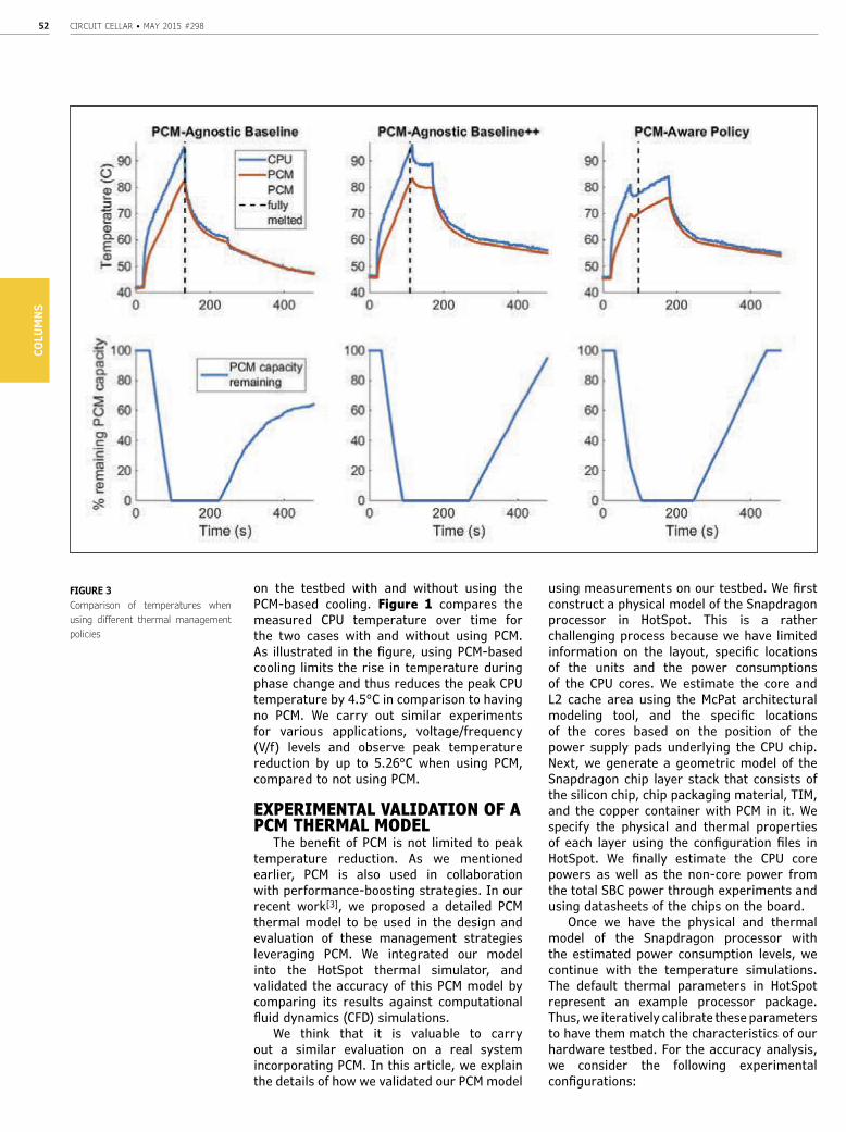
CIRCUIT CELLAR • MAY 2015 #29852CO
LUM
NS
on the testbed with and without using the PCM-based cooling. Figure 1 compares the measured CPU temperature over time for the two cases with and without using PCM. As illustrated in the figure, using PCM-based cooling limits the rise in temperature during phase change and thus reduces the peak CPU temperature by 4.5°C in comparison to having no PCM. We carry out similar experiments for various applications, voltage/frequency (V/f) levels and observe peak temperature reduction by up to 5.26°C when using PCM, compared to not using PCM.
EXPERIMENTAL VALIDATION OF A PCM THERMAL MODEL
The benefit of PCM is not limited to peak temperature reduction. As we mentioned earlier, PCM is also used in collaboration with performance-boosting strategies. In our recent work[3], we proposed a detailed PCM thermal model to be used in the design and evaluation of these management strategies leveraging PCM. We integrated our model into the HotSpot thermal simulator, and validated the accuracy of this PCM model by comparing its results against computational fluid dynamics (CFD) simulations.
We think that it is valuable to carry out a similar evaluation on a real system incorporating PCM. In this article, we explain the details of how we validated our PCM model
using measurements on our testbed. We first construct a physical model of the Snapdragon processor in HotSpot. This is a rather challenging process because we have limited information on the layout, specific locations of the units and the power consumptions of the CPU cores. We estimate the core and L2 cache area using the McPat architectural modeling tool, and the specific locations of the cores based on the position of the power supply pads underlying the CPU chip. Next, we generate a geometric model of the Snapdragon chip layer stack that consists of the silicon chip, chip packaging material, TIM, and the copper container with PCM in it. We specify the physical and thermal properties of each layer using the configuration files in HotSpot. We finally estimate the CPU core powers as well as the non-core power from the total SBC power through experiments and using datasheets of the chips on the board.
Once we have the physical and thermal model of the Snapdragon processor with the estimated power consumption levels, we continue with the temperature simulations. The default thermal parameters in HotSpot represent an example processor package. Thus, we iteratively calibrate these parameters to have them match the characteristics of our hardware testbed. For the accuracy analysis, we consider the following experimental configurations:
FIGURE 3Comparison of temperatures when using different thermal management policies

such as this book,
designing a microprocessor can be easy. Okay, maybe not easy, but certainly less complicated. Monte Dalrymple has taken his years of experience designing embedded architecture and microprocessors and compiled his knowledge into one comprehensive guide to processor design in the real world.
cc-webshop.com
Microprocessor Design Using Verilog HDL will provide you with information about:
• Verilog HDL Review
• Verilog Coding Style
• Design Work
• Microarchitecture
• Writing in Verilog
• Debugging, Verification, and Testing
• Post Simulation and more!
Verilog HDLWith the right tools
Monte demonstrates how Verilog hardware description language (HDL) enables you to depict, simulate, and synthesize an electronic design so you can reduce your workload and increase productivity.
CIRCUIT CELLAR • MAY 2015 #29854CO
LUM
NS
• We have four different CPU frequency settings: 594, 810, 1026, and 1242 MHz
• We activate different number of CPU cores: one, two, three, and four cores
• We run three applications: successive over-relaxation (sor), sparse matrix multiplication (smult), and lower-upper factorization (lu).
For each combination of the configurations listed above, we run the experiments and collect measurement and simulation data from the testbed and HotSpot, respectively. In Figure 2, we report the transient temperature error probability of the HotSpot PCM model on a histogram plot. The x-axis represents
the temperature error intervals in degrees Celsius and y-axis shows the probability of having a temperature error within the corresponding interval. The plot shows that the transient temperature error between the measured and simulated temperature is less than 3°C with 0.914 probability. On the other hand, probability of having an error that is higher than 6°C is as low as 0.008.
PCM-AWARE THERMAL MANAGEMENT
To design thermal management policies that efficiently utilize the latent heat capacity of PCM, it is important to know the remaining PCM capacity at runtime. For this purpose, we implement a soft PCM capacity sensor that monitors how much of the PCM remains un-melted. The PCM capacity sensor is implemented in the software running on the testbed, and consists of a counter that accumulates the amount of latent heat energy stored in the PCM over time, during phase change. At the beginning of the phase transition from solid to liquid, the amount of latent heat energy stored in the PCM is zero. When fully melted, the PCM will have stored a quantity of energy equal to the PCM’s latent heat of fusion. By leveraging the temperature information from the on-chip temperature sensors, the PCM temperature sensor, and the ambient air temperature, the PCM capacity sensor estimates the amount of heat entering the PCM (dissipated from the CPU), and the amount of heat exiting the PCM via convection to the ambient air.
We test PCM-aware thermal management schemes, which decide CPU clock frequency settings based on the remaining PCM capacity, and compare them to thermal management schemes which rely solely on the CPU temperature to make decisions on whether to turn off CPU cores or lower the CPU clock frequency to mitigate high CPU temperatures. We implement the following thermal management policies for comparison:
• PCM-Agnostic baseline: As our baseline policy, we implement the computational sprinting policy from prior work.[2] In this policy, during sprinting mode, all four cores are active and set to maximum CPU clock frequency (1,242 MHz) until any one core reaches a critical temperature of 95°C. At this point, the system switches to a sustained mode where all workload is migrated to a single CPU core, and the rest of the cores are turned off to allow the CPU temperature to drop.
• PCM-Aware: A policy proposed in prior work,[4] where the system switches to a lower-intensity sprinting mode when the remaining
ABOUT THE AUTHORFulya Kaplan ([email protected]) is currently a PhD candidate in the Electrical and Computer Engineering Department at Boston University. She received her BS degree in Electrical and Electronics Engineering from the Middle East Technical University, Turkey, in 2011. Her research interests are temperature and energy management in multicore processors and data centers. She is a student member of the IEEE. Charlie De Vivero ([email protected]) is a software engineer at Raytheon Com-pany. His expertise lies in the design and development of embedded systems solutions, and has experience with a variety of technologies ranging from small spacecraft systems, to large-scale ballistic missile defense systems. He received a BS degree in Aerospace Engineering from the Massachusetts Institute of Technology in 2011 and an MS degree in Computer Engineering from Boston University in 2015.
circuitcellar.com/ccmaterials
REFERENCES[1] M. B. Taylor, “A Land-scape of the New Dark Silicon Design,” IEEE MICRO, Vol. 33, September–October 2013.
[2] A. Raghavan, Y. Luo, A. Chandawalla, M. Papaefthymi-ou, K. P. Pipe, T. F. Wenisch, M. M. K. Martin, “Computa-tional Sprinting,” Interna-tional Symposium on High
Performance Computer Architecture (HPCA), 2012, pp. 1-12.
[3] F. Kaplan, C. De Vivero, S. Howes, M. Aro-ra, H. Homayoun, W. Burleson, D. Tullsen, and A. K. Coskun, “Modeling and Analysis of Phase Change Materials for Efficient Thermal Man-agement,” International Conference on Com-puter Design (ICCD), 2014.
[4] A. Raghavan, L. Emurian, L. Shao, M. Pa-paefthymiou, K. P. Pipe, T. F. Wenisch, and M. M. K. Martin, “Computational Sprinting on a Hardware/Software Testbed,” International Conference on Architectural Support for Pro-gramming Languages and Operating Systems (ASPLOS), 2013.
SOURCEIFC6410 SBCInforce Computing | www.inforcecomputing.com
circuitcellar.com 55COLUM
NS
PCM capacity falls below 25%. During the lower-intensity sprinting mode, all four cores remain active, but the frequency is lowered to 1,026 MHz.
• PCM-Agnostic baseline++: We implement a variation of the PCM-agnostic baseline policy, but instead of turning off cores, the system switches to a lower-intensity sprinting mode when any one core reaches a critical temperature of 95°C.
To demonstrate the performance of these policies, we run the sor application, which is a computationally-intensive benchmark, repeatedly a fixed number of times. We define the performance gain of the PCM-aware and PCM-agnostic baseline++ policies as the percent reduction in application execution time compared to when using the PCM-agnostic baseline policy.
As you can see in Figure 3, the PCM-aware policy offers a 30% faster execution time than the PCM-agnostic baseline policy by adjusting the sprint intensity based on remaining PCM capacity, thus extending the sprinting duration. The PCM-agnostic baseline++ policy offers the fastest execution time (34% faster), since most of the time is spent sprinting. However, using the PCM-agnostic baseline++ policy results in higher average CPU and PCM temperatures. For most of the application running time, the PCM remains in a fully melted state. The PCM-aware policy sacrifices a 4% performance gain compared to the PCM-agnostic baseline++, but allows the CPU to operate at a 12°C lower peak temperature and 4.45°C lower average temperature. By keeping the CPU and PCM temperatures lower, the PCM-aware policy allows the PCM to start freezing back earlier, compared to when using the PCM-agnostic baseline++ policy.
RESULTSWe have designed and built a hardware
testbed with a PCM container installed on top of the package. We experimentally validate our previously proposed phase change thermal model using measurements from the testbed. Our transient simulations show that the error between the measured and simulated temperatures is less than 3°C with a 0.914 probability. We also implement a soft PCM capacity sensor to monitor the amount of un-melted PCM at runtime. We use the PCM capacity sensor as part of a PCM-aware thermal management policy and demonstrate the benefits of using such a policy. Experimental evaluation shows that the PCM-aware policy provides up to a 30% better performance compared to the PCM-agnostic baseline policy.
©2015 Measurement Computing Corporation, 10 Commerce Way, Norton, MA 02766 • [email protected]
1.800.234.4232Contact us
mccdaq.com
M E A S U R E M E N T C O M P U T I N G
Easy to Use • Easy to Integrate • Easy to Support
Great 16-BitDAQ Solutions
NEW
Ethernet, MultifunctionE-1608Only $499• 8 SE/4 DIFF analog inputs• 250 kS/s sample rate• 2 analog outputs• 8 digital I/O, 1 counter
Low-Cost, MultifunctionUSB-231Only $249• 8 SE/4 DIFF analog inputs• 50 kS/s sample rate• 2 analog outputs• 8 digital I/O, 1 counter
Simultaneous SamplingUSB-1602HSOnly $1,999• 2 SE analog inputs• 2 MS/s sample rate• 3 quadrature detectors• 4 counters
Simultaneous SamplingUSB-1608FS-PlusOnly $399• 8 simultaneous analog inputs• 400 kS/s overall sample rate• 100 kS/s max for any channel• 8 digital I/O, 1 counter
High-Channel CountUSB-2533Only $1,149• 64 SE/32 DIFF analog inputs• 1 MS/s sample rate• 2 timer outputs• 24 digital I/O, 4 counters
High-Speed, MultifunctionUSB-1608GX-2AOOnly $799• 16 SE/8 DIFF analog inputs• 500 kS/s sample rate• 2 analog outputs• 8 digital I/O, 2 counters
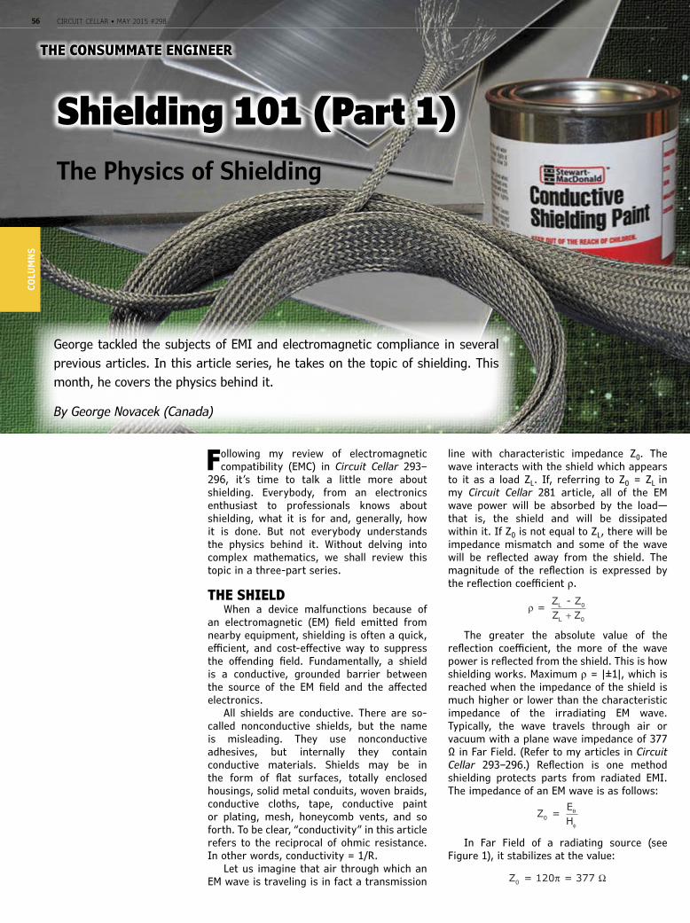
CIRCUIT CELLAR • MAY 2015 #29856CO
LUM
NS
THE CONSUMMATE ENGINEER
Following my review of electromagnetic compatibility (EMC) in Circuit Cellar 293–
296, it’s time to talk a little more about shielding. Everybody, from an electronics enthusiast to professionals knows about shielding, what it is for and, generally, how it is done. But not everybody understands the physics behind it. Without delving into complex mathematics, we shall review this topic in a three-part series.
THE SHIELDWhen a device malfunctions because of
an electromagnetic (EM) field emitted from nearby equipment, shielding is often a quick, efficient, and cost-effective way to suppress the offending field. Fundamentally, a shield is a conductive, grounded barrier between the source of the EM field and the affected electronics.
All shields are conductive. There are so-called nonconductive shields, but the name is misleading. They use nonconductive adhesives, but internally they contain conductive materials. Shields may be in the form of flat surfaces, totally enclosed housings, solid metal conduits, woven braids, conductive cloths, tape, conductive paint or plating, mesh, honeycomb vents, and so forth. To be clear, “conductivity” in this article refers to the reciprocal of ohmic resistance. In other words, conductivity = 1/R.
Let us imagine that air through which an EM wave is traveling is in fact a transmission
line with characteristic impedance Z0. The wave interacts with the shield which appears to it as a load ZL. If, referring to Z0 = ZL in my Circuit Cellar 281 article, all of the EM wave power will be absorbed by the load— that is, the shield and will be dissipated within it. If Z0 is not equal to ZL, there will be impedance mismatch and some of the wave will be reflected away from the shield. The magnitude of the reflection is expressed by the reflection coefficient ρ.
ρ = Z - ZL 0
Z ZL + 0
The greater the absolute value of the reflection coefficient, the more of the wave power is reflected from the shield. This is how shielding works. Maximum ρ = |±1|, which is reached when the impedance of the shield is much higher or lower than the characteristic impedance of the irradiating EM wave. Typically, the wave travels through air or vacuum with a plane wave impedance of 377 Ω in Far Field. (Refer to my articles in Circuit Cellar 293–296.) Reflection is one method shielding protects parts from radiated EMI. The impedance of an EM wave is as follows:
Z = 0EH
θ
φ
In Far Field of a radiating source (see Figure 1), it stabilizes at the value:
Z = 120 = 377 0 π Ω
Shielding 101 (Part 1)
George tackled the subjects of EMI and electromagnetic compliance in several previous articles. In this article series, he takes on the topic of shielding. This month, he covers the physics behind it.
By George Novacek (Canada)
The Physics of Shielding
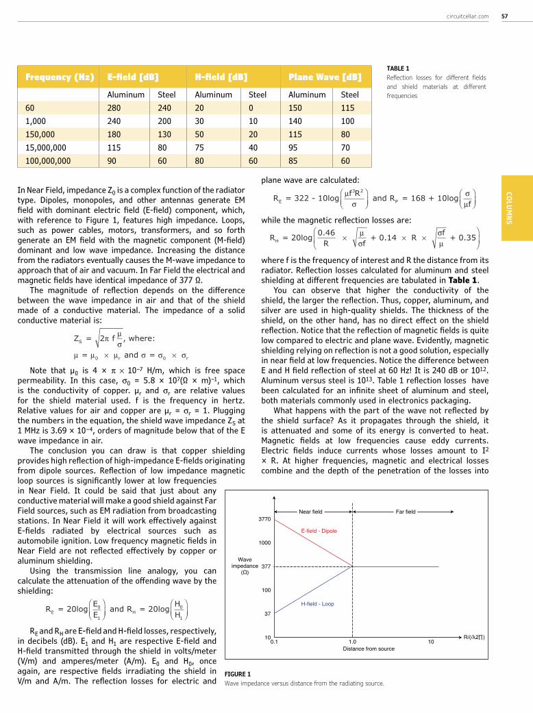
circuitcellar.com 57COLUM
NS
In Near Field, impedance Z0 is a complex function of the radiator type. Dipoles, monopoles, and other antennas generate EM field with dominant electric field (E-field) component, which, with reference to Figure 1, features high impedance. Loops, such as power cables, motors, transformers, and so forth generate an EM field with the magnetic component (M-field) dominant and low wave impedance. Increasing the distance from the radiators eventually causes the M-wave impedance to approach that of air and vacuum. In Far Field the electrical and magnetic fields have identical impedance of 377 Ω.
The magnitude of reflection depends on the difference between the wave impedance in air and that of the shield made of a conductive material. The impedance of a solid conductive material is:
Z = f , where:
= and = 0 r 0 r
S 2π µσ
µ µ µ σ σ σ× ×
Note that µ0 is 4 × π × 10–7 H/m, which is free space permeability. In this case, σ0 = 5.8 × 10⁷(Ω × m)–1, which is the conductivity of copper. µr and σr are relative values for the shield material used. f is the frequency in hertz. Relative values for air and copper are µr = σr = 1. Plugging the numbers in the equation, the shield wave impedance ZS at 1 MHz is 3.69 × 10⁻⁴, orders of magnitude below that of the E wave impedance in air.
The conclusion you can draw is that copper shielding provides high reflection of high-impedance E-fields originating from dipole sources. Reflection of low impedance magnetic loop sources is significantly lower at low frequencies in Near Field. It could be said that just about any conductive material will make a good shield against Far Field sources, such as EM radiation from broadcasting stations. In Near Field it will work effectively against E-fields radiated by electrical sources such as automobile ignition. Low frequency magnetic fields in Near Field are not reflected effectively by copper or aluminum shielding.
Using the transmission line analogy, you can calculate the attenuation of the offending wave by the shielding:
R EE
HHE H = 20log and R = 20log0
1
0
1
⎛⎝⎜
⎞⎠⎟
⎛⎝⎜
⎞⎠⎟
RE and RH are E-field and H-field losses, respectively, in decibels (dB). E1 and H1 are respective E-field and H-field transmitted through the shield in volts/meter (V/m) and amperes/meter (A/m). E0 and H0, once again, are respective fields irradiating the shield in V/m and A/m. The reflection losses for electric and
plane wave are calculated:
R f R RfE P = 322 - 10log and = 168 + 10logµ
σσµ
3 2⎛⎝⎜
⎞⎠⎟
⎛⎝⎜
⎞⎠⎟
while the magnetic reflection losses are:
RR f
fH = 20log + 0.14 R + 0.350 46. × × ×
⎛
⎝⎜⎞
⎠⎟µσ
σµ
where f is the frequency of interest and R the distance from its radiator. Reflection losses calculated for aluminum and steel shielding at different frequencies are tabulated in Table 1.
You can observe that higher the conductivity of the shield, the larger the reflection. Thus, copper, aluminum, and silver are used in high-quality shields. The thickness of the shield, on the other hand, has no direct effect on the shield reflection. Notice that the reflection of magnetic fields is quite low compared to electric and plane wave. Evidently, magnetic shielding relying on reflection is not a good solution, especially in near field at low frequencies. Notice the difference between E and H field reflection of steel at 60 Hz! It is 240 dB or 1012. Aluminum versus steel is 1013. Table 1 reflection losses have been calculated for an infinite sheet of aluminum and steel, both materials commonly used in electronics packaging.
What happens with the part of the wave not reflected by the shield surface? As it propagates through the shield, it is attenuated and some of its energy is converted to heat. Magnetic fields at low frequencies cause eddy currents. Electric fields induce currents whose losses amount to I2 × R. At higher frequencies, magnetic and electrical losses combine and the depth of the penetration of the losses into
FIGURE 1Wave impedance versus distance from the radiating source.
3770
1000
377
100
37
10Distance from source
Waveimpedance
(Ω)
R/(/λ2∏)
Near field Far field
E-field - Dipole
H-field - Loop
0.1 1.0 10
TABLE 1Reflection losses for different fields and shield materials at different frequencies
Frequency (Hz) E-field [dB] H-field [dB] Plane Wave [dB]
Aluminum Steel Aluminum Steel Aluminum Steel60 280 240 20 0 150 1151,000 240 200 30 10 140 100150,000 180 130 50 20 115 8015,000,000 115 80 75 40 95 70100,000,000 90 60 80 60 85 60
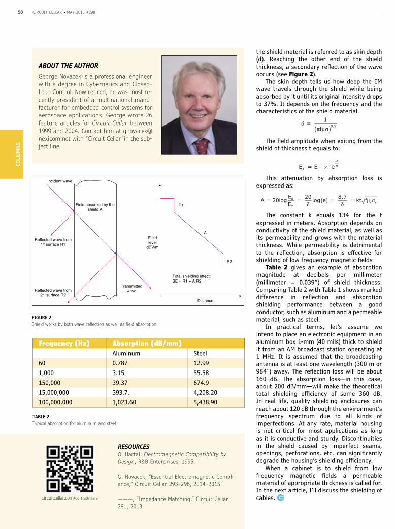
CIRCUIT CELLAR • MAY 2015 #29858CO
LUM
NS
the shield material is referred to as skin depth (d). Reaching the other end of the shield thickness, a secondary reflection of the wave occurs (see Figure 2).
The skin depth tells us how deep the EM wave travels through the shield while being absorbed by it until its original intensity drops to 37%. It depends on the frequency and the characteristics of the shield material.
δπ µσ
= 10 5f( ) .
The field amplitude when exiting from the shield of thickness t equals to:
E = E eT 0 ×−tσ
This attenuation by absorption loss is expressed as:
A = 20log EE
= = = kt0
Tr re f20 8 7
δ δµ σlog .( )
The constant k equals 134 for the t expressed in meters. Absorption depends on conductivity of the shield material, as well as its permeability and grows with the material thickness. While permeability is detrimental to the reflection, absorption is effective for shielding of low frequency magnetic fields
Table 2 gives an example of absorption magnitude at decibels per millimeter (millimeter = 0.039″) of shield thickness. Comparing Table 2 with Table 1 shows marked difference in reflection and absorption shielding performance between a good conductor, such as aluminum and a permeable material, such as steel.
In practical terms, let’s assume we intend to place an electronic equipment in an aluminum box 1-mm (40 mils) thick to shield it from an AM broadcast station operating at 1 MHz. It is assumed that the broadcasting antenna is at least one wavelength (300 m or 984´) away. The reflection loss will be about 160 dB. The absorption loss—in this case, about 200 dB/mm—will make the theoretical total shielding efficiency of some 360 dB. In real life, quality shielding enclosures can reach about 120 dB through the environment’s frequency spectrum due to all kinds of imperfections. At any rate, material housing is not critical for most applications as long as it is conductive and sturdy. Discontinuities in the shield caused by imperfect seams, openings, perforations, etc. can significantly degrade the housing’s shielding efficiency.
When a cabinet is to shield from low frequency magnetic fields a permeable material of appropriate thickness is called for. In the next article, I’ll discuss the shielding of cables. circuitcellar.com/ccmaterials
RESOURCESO. Hartal, Electromagnetic Compatibility by Design, R&B Enterprises, 1995.
G. Novacek, “Essential Electromagnetic Compli-ance,” Circuit Cellar 293–296, 2014–2015.
———, “Impedance Matching,” Circuit Cellar 281, 2013.
ABOUT THE AUTHORGeorge Novacek is a professional engineer with a degree in Cybernetics and Closed-Loop Control. Now retired, he was most re-cently president of a multinational manu-facturer for embedded control systems for aerospace applications. George wrote 26 feature articles for Circuit Cellar between 1999 and 2004. Contact him at [email protected] with “Circuit Cellar”in the sub-ject line.
FIGURE 2Shield works by both wave reflection as well as field absorption
Incident wave
Reflected wave from2nd surface R2
Reflected wave from1st surface R1
Field absorbed by theshield A
Transmittedwave
Distance
Total shielding effect:SE = R1 + A R2
Fieldlevel
dBV/m
R1
R2
A
Frequency (Hz) Absorption (dB/mm)Aluminum Steel
60 0.787 12.991,000 3.15 55.58150,000 39.37 674.915,000,000 393.7. 4,208.20100,000,000 1,023.60 5,438.90
TABLE 2Typical absorption for aluminum and steel

OPEN
RUGGED
LONG LIFE
ORIGIN
ALUnique embedded solutions add value for our customers
Support every step of the way with open source vision
Embedded systems that are built to endure
We’ve never discontinued a product in 30 years
DESIGN YOUR SOLUTION TODAYCALL 480-837-5200
TS-TPC-8390 Panel PCTouchscreen with Linux & Android
Series start at
$422Qty 1
Qty 100
$389
Up to 1 GHz Freescale i.MX6 ARM Quad CPU
Headphone Connector and Speakers
2x Ethernet, 2x USB Host Ports
2x microSD Card Sockets for Redundant Storage
DIO, RS-232, RS-485, TTL UARTs, I2C, 12S, CAN, ModBus
Up to 2 GB DDR3 RAM, 4 GB eMMC Flash
Optional WiFi, Bluetooth, GPS, Cellular, XBEE Modules
Resistive and Capacitive Touchscreens
Features can include:
TS-4600: 450 MHz low cost w/ 2 EthernetsTS-4710: Up to 1 GHz PXA168 w/ videoTS-4720: Like TS-4710 + 2 GB eMMC Flash & 2 EthernetsTS-4200: Atmel ARM9 w/ super low powerTS-4800: 800 MHz FreeScale iMX515 w/ video
Computer-on-ModulesState of the Art Embedded Design
TS-7400-V2 Single Board ComputerLow Cost and Low Power
Pricing Starts At
$117Qty 1
Qty 100
$84
-40 ºC to 85 ºC industrial temperature range
Easy development w/ Debian and Linux Preinstalled
High data reliability with 2 GB SLC eMMC flash
Several control I/O interfaces
Easily enable low power applications using software
Benefits:
Fastboot launches your application quickly
454 MHz ARM CPU
128 to 256 MB RAM
1x USB Host
2x RS-232, 2x TTL Ports
1x microSD Socket
2 GB eMMC Flash
39x DIO, 1x CAN
4x ADC Ports
1x 10/100 Ethernet 0.5 W Low Power Mode
Features:
Available with TS-ENC740 enclosure
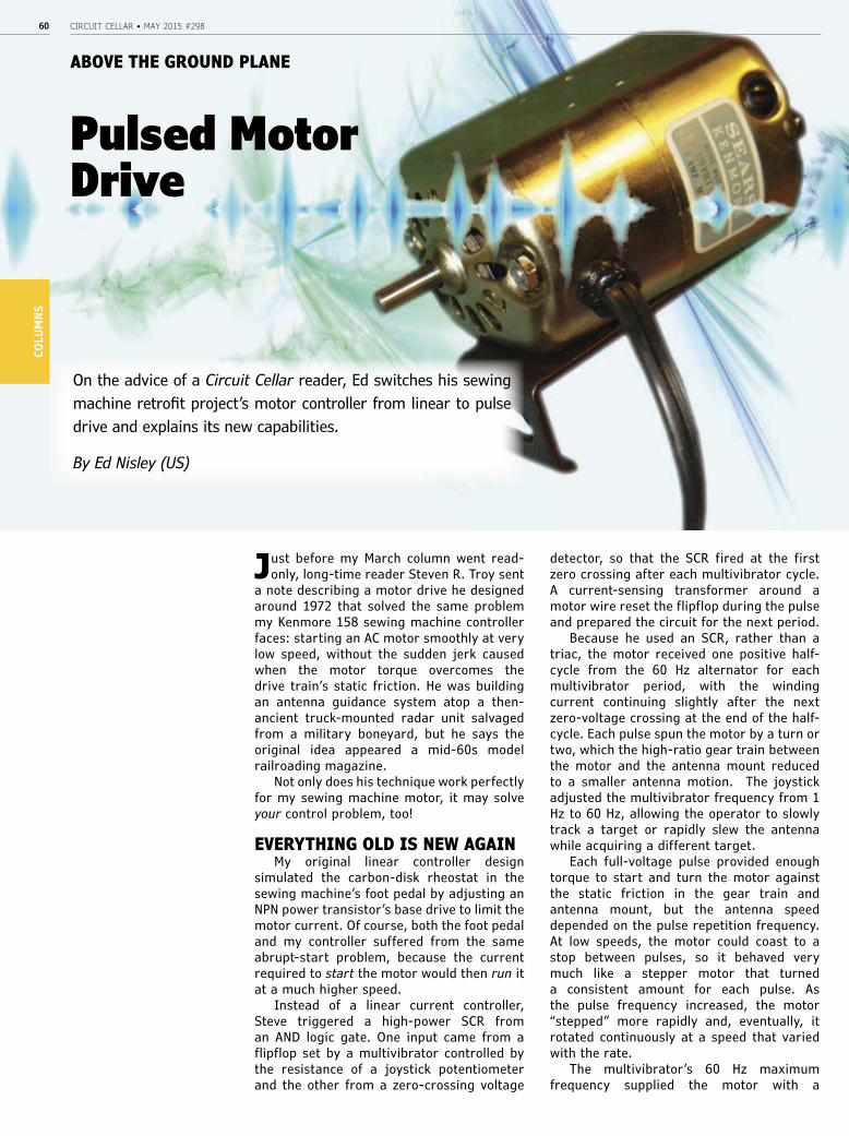
CIRCUIT CELLAR • MAY 2015 #29860CO
LUM
NS
Just before my March column went read-only, long-time reader Steven R. Troy sent
a note describing a motor drive he designed around 1972 that solved the same problem my Kenmore 158 sewing machine controller faces: starting an AC motor smoothly at very low speed, without the sudden jerk caused when the motor torque overcomes the drive train’s static friction. He was building an antenna guidance system atop a then-ancient truck-mounted radar unit salvaged from a military boneyard, but he says the original idea appeared a mid-60s model railroading magazine.
Not only does his technique work perfectly for my sewing machine motor, it may solve your control problem, too!
EVERYTHING OLD IS NEW AGAINMy original linear controller design
simulated the carbon-disk rheostat in the sewing machine’s foot pedal by adjusting an NPN power transistor’s base drive to limit the motor current. Of course, both the foot pedal and my controller suffered from the same abrupt-start problem, because the current required to start the motor would then run it at a much higher speed.
Instead of a linear current controller, Steve triggered a high-power SCR from an AND logic gate. One input came from a flipflop set by a multivibrator controlled by the resistance of a joystick potentiometer and the other from a zero-crossing voltage
detector, so that the SCR fired at the first zero crossing after each multivibrator cycle. A current-sensing transformer around a motor wire reset the flipflop during the pulse and prepared the circuit for the next period.
Because he used an SCR, rather than a triac, the motor received one positive half-cycle from the 60 Hz alternator for each multivibrator period, with the winding current continuing slightly after the next zero-voltage crossing at the end of the half-cycle. Each pulse spun the motor by a turn or two, which the high-ratio gear train between the motor and the antenna mount reduced to a smaller antenna motion. The joystick adjusted the multivibrator frequency from 1 Hz to 60 Hz, allowing the operator to slowly track a target or rapidly slew the antenna while acquiring a different target.
Each full-voltage pulse provided enough torque to start and turn the motor against the static friction in the gear train and antenna mount, but the antenna speed depended on the pulse repetition frequency. At low speeds, the motor could coast to a stop between pulses, so it behaved very much like a stepper motor that turned a consistent amount for each pulse. As the pulse frequency increased, the motor “stepped” more rapidly and, eventually, it rotated continuously at a speed that varied with the rate.
The multivibrator’s 60 Hz maximum frequency supplied the motor with a
ABOVE THE GROUND PLANE
Pulsed Motor Drive
On the advice of a Circuit Cellar reader, Ed switches his sewing machine retrofit project’s motor controller from linear to pulse drive and explains its new capabilities.
By Ed Nisley (US)
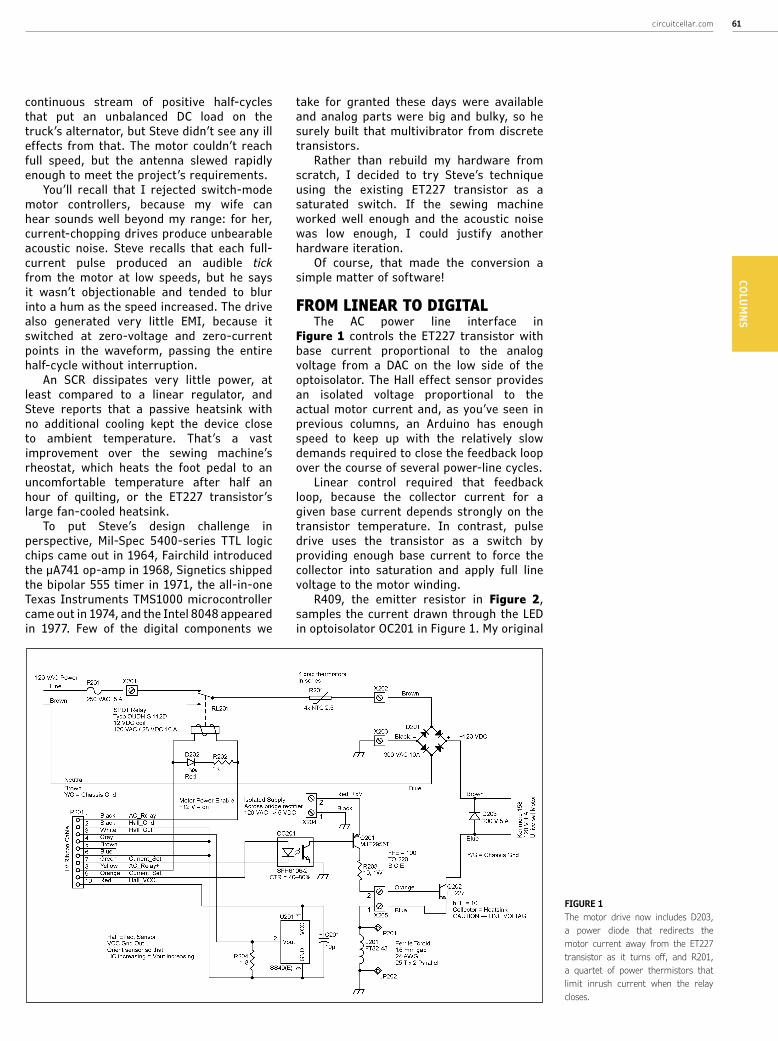
circuitcellar.com 61COLUM
NS
continuous stream of positive half-cycles that put an unbalanced DC load on the truck’s alternator, but Steve didn’t see any ill effects from that. The motor couldn’t reach full speed, but the antenna slewed rapidly enough to meet the project’s requirements.
You’ll recall that I rejected switch-mode motor controllers, because my wife can hear sounds well beyond my range: for her, current-chopping drives produce unbearable acoustic noise. Steve recalls that each full-current pulse produced an audible tick from the motor at low speeds, but he says it wasn’t objectionable and tended to blur into a hum as the speed increased. The drive also generated very little EMI, because it switched at zero-voltage and zero-current points in the waveform, passing the entire half-cycle without interruption.
An SCR dissipates very little power, at least compared to a linear regulator, and Steve reports that a passive heatsink with no additional cooling kept the device close to ambient temperature. That’s a vast improvement over the sewing machine’s rheostat, which heats the foot pedal to an uncomfortable temperature after half an hour of quilting, or the ET227 transistor’s large fan-cooled heatsink.
To put Steve’s design challenge in perspective, Mil-Spec 5400-series TTL logic chips came out in 1964, Fairchild introduced the µA741 op-amp in 1968, Signetics shipped the bipolar 555 timer in 1971, the all-in-one Texas Instruments TMS1000 microcontroller came out in 1974, and the Intel 8048 appeared in 1977. Few of the digital components we
take for granted these days were available and analog parts were big and bulky, so he surely built that multivibrator from discrete transistors.
Rather than rebuild my hardware from scratch, I decided to try Steve’s technique using the existing ET227 transistor as a saturated switch. If the sewing machine worked well enough and the acoustic noise was low enough, I could justify another hardware iteration.
Of course, that made the conversion a simple matter of software!
FROM LINEAR TO DIGITALThe AC power line interface in
Figure 1 controls the ET227 transistor with base current proportional to the analog voltage from a DAC on the low side of the optoisolator. The Hall effect sensor provides an isolated voltage proportional to the actual motor current and, as you’ve seen in previous columns, an Arduino has enough speed to keep up with the relatively slow demands required to close the feedback loop over the course of several power-line cycles.
Linear control required that feedback loop, because the collector current for a given base current depends strongly on the transistor temperature. In contrast, pulse drive uses the transistor as a switch by providing enough base current to force the collector into saturation and apply full line voltage to the motor winding.
R409, the emitter resistor in Figure 2, samples the current drawn through the LED in optoisolator OC201 in Figure 1. My original
FIGURE 1 The motor drive now includes D203, a power diode that redirects the motor current away from the ET227 transistor as it turns off, and R201, a quartet of power thermistors that limit inrush current when the relay closes.
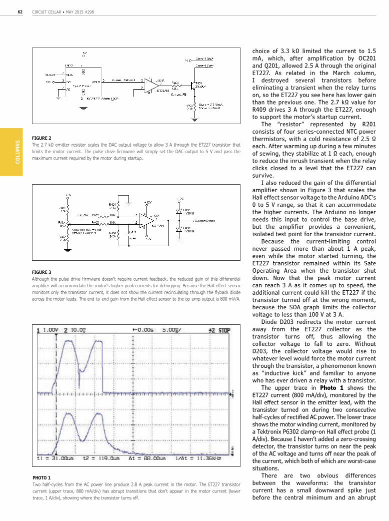
CIRCUIT CELLAR • MAY 2015 #29862CO
LUM
NS
choice of 3.3 kΩ limited the current to 1.5 mA, which, after amplification by OC201 and Q201, allowed 2.5 A through the original ET227. As related in the March column, I destroyed several transistors before eliminating a transient when the relay turns on, so the ET227 you see here has lower gain than the previous one. The 2.7 kΩ value for R409 drives 3 A through the ET227, enough to support the motor’s startup current.
The “resistor” represented by R201 consists of four series-connected NTC power thermistors, with a cold resistance of 2.5 Ω each. After warming up during a few minutes of sewing, they stabilize at 1 Ω each, enough to reduce the inrush transient when the relay clicks closed to a level that the ET227 can survive.
I also reduced the gain of the differential amplifier shown in Figure 3 that scales the Hall effect sensor voltage to the Arduino ADC’s 0 to 5 V range, so that it can accommodate the higher currents. The Arduino no longer needs this input to control the base drive, but the amplifier provides a convenient, isolated test point for the transistor current.
Because the current-limiting control never passed more than about 1 A peak, even while the motor started turning, the ET227 transistor remained within its Safe Operating Area when the transistor shut down. Now that the peak motor current can reach 3 A as it comes up to speed, the additional current could kill the ET227 if the transistor turned off at the wrong moment, because the SOA graph limits the collector voltage to less than 100 V at 3 A.
Diode D203 redirects the motor current away from the ET227 collector as the transistor turns off, thus allowing the collector voltage to fall to zero. Without D203, the collector voltage would rise to whatever level would force the motor current through the transistor, a phenomenon known as “inductive kick” and familiar to anyone who has ever driven a relay with a transistor.
The upper trace in Photo 1 shows the ET227 current (800 mA/div), monitored by the Hall effect sensor in the emitter lead, with the transistor turned on during two consecutive half-cycles of rectified AC power. The lower trace shows the motor winding current, monitored by a Tektronix P6302 clamp-on Hall effect probe (1 A/div). Because I haven’t added a zero-crossing detector, the transistor turns on near the peak of the AC voltage and turns off near the peak of the current, which both of which are worst-case situations.
There are two obvious differences between the waveforms: the transistor current has a small downward spike just before the central minimum and an abrupt
PHOTO 1Two half-cycles from the AC power line produce 2.8 A peak current in the motor. The ET227 transistor current (upper trace, 800 mA/div) has abrupt transitions that don’t appear in the motor current (lower trace, 1 A/div), showing where the transistor turns off.
FIGURE 2 The 2.7 kΩ emitter resistor scales the DAC output voltage to allow 3 A through the ET227 transistor that limits the motor current. The pulse drive firmware will simply set the DAC output to 5 V and pass the maximum current required by the motor during startup.
FIGURE 3Although the pulse drive firmware doesn’t require current feedback, the reduced gain of this differential amplifier will accommodate the motor’s higher peak currents for debugging. Because the Hall effect sensor monitors only the transistor current, it does not show the current recirculating through the flyback diode across the motor leads. The end-to-end gain from the Hall effect sensor to the op-amp output is 800 mV/A.
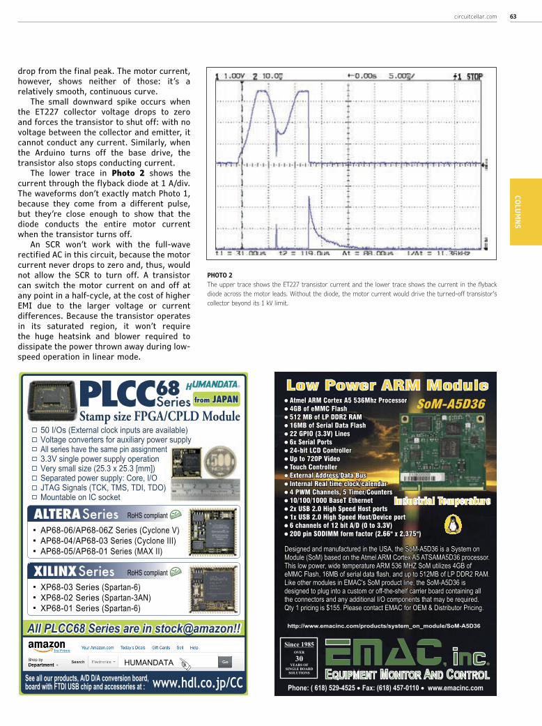
circuitcellar.com 63COLUM
NS
drop from the final peak. The motor current, however, shows neither of those: it’s a relatively smooth, continuous curve.
The small downward spike occurs when the ET227 collector voltage drops to zero and forces the transistor to shut off: with no voltage between the collector and emitter, it cannot conduct any current. Similarly, when the Arduino turns off the base drive, the transistor also stops conducting current.
The lower trace in Photo 2 shows the current through the flyback diode at 1 A/div. The waveforms don’t exactly match Photo 1, because they come from a different pulse, but they’re close enough to show that the diode conducts the entire motor current when the transistor turns off.
An SCR won’t work with the full-wave rectified AC in this circuit, because the motor current never drops to zero and, thus, would not allow the SCR to turn off. A transistor can switch the motor current on and off at any point in a half-cycle, at the cost of higher EMI due to the larger voltage or current differences. Because the transistor operates in its saturated region, it won’t require the huge heatsink and blower required to dissipate the power thrown away during low-speed operation in linear mode.
PHOTO 2The upper trace shows the ET227 transistor current and the lower trace shows the current in the flyback diode across the motor leads. Without the diode, the motor current would drive the turned-off transistor’s collector beyond its 1 kV limit.
HUMANDATA
All PLCC68 Series are in stock@amazon!!All PLCC68 Series are in stock@amazon!!
Stamp size FPGA/CPLD Module
See all our products, A/D D/A conversion board, board with FTDI USB chip and accessories at : www.hdl.co.jp/CC
50 I/Os (External clock inputs are available)Voltage converters for auxiliary power supplyAll series have the same pin assignment3.3V single power supply operationVery small size (25.3 x 25.3 [mm])Separated power supply: Core, I/OJTAG Signals (TCK, TMS, TDI, TDO)Mountable on IC socket
XILINX Series RoHS compliant
XP68-03 Series (Spartan-6)XP68-02 Series (Spartan-3AN)XP68-01 Series (Spartan-6)
ALTERA Series RoHS compliant
AP68-06/AP68-06Z Series (Cyclone V)AP68-04/AP68-03 Series (Cyclone III)AP68-05/AP68-01 Series (MAX II)
from JAPAN from JAPAN SeriesPLCC68
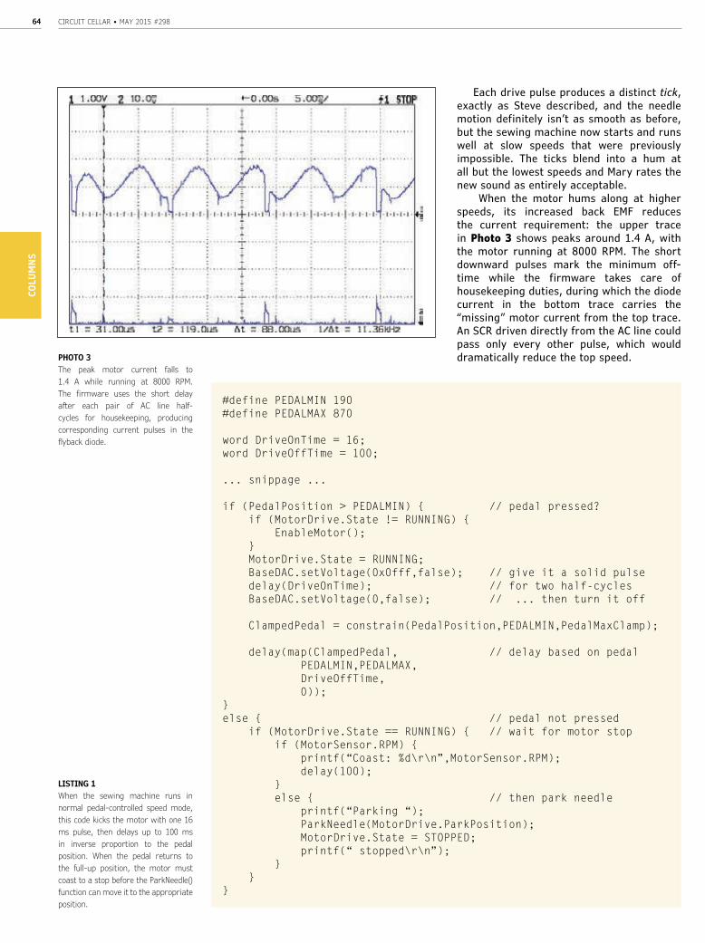
CIRCUIT CELLAR • MAY 2015 #29864CO
LUM
NS
Each drive pulse produces a distinct tick, exactly as Steve described, and the needle motion definitely isn’t as smooth as before, but the sewing machine now starts and runs well at slow speeds that were previously impossible. The ticks blend into a hum at all but the lowest speeds and Mary rates the new sound as entirely acceptable.
When the motor hums along at higher speeds, its increased back EMF reduces the current requirement: the upper trace in Photo 3 shows peaks around 1.4 A, with the motor running at 8000 RPM. The short downward pulses mark the minimum off-time while the firmware takes care of housekeeping duties, during which the diode current in the bottom trace carries the “missing” motor current from the top trace. An SCR driven directly from the AC line could pass only every other pulse, which would dramatically reduce the top speed.
LISTING 1When the sewing machine runs in normal pedal-controlled speed mode, this code kicks the motor with one 16 ms pulse, then delays up to 100 ms in inverse proportion to the pedal position. When the pedal returns to the full-up position, the motor must coast to a stop before the ParkNeedle() function can move it to the appropriate position.
#define PEDALMIN 190#define PEDALMAX 870
word DriveOnTime = 16;word DriveOffTime = 100;
... snippage ...
if (PedalPosition > PEDALMIN) // pedal pressed? if (MotorDrive.State != RUNNING) EnableMotor(); MotorDrive.State = RUNNING; BaseDAC.setVoltage(0x0fff,false); // give it a solid pulse delay(DriveOnTime); // for two half-cycles BaseDAC.setVoltage(0,false); // ... then turn it off
ClampedPedal = constrain(PedalPosition,PEDALMIN,PedalMaxClamp);
delay(map(ClampedPedal, // delay based on pedal PEDALMIN,PEDALMAX, DriveOffTime, 0));else // pedal not pressed if (MotorDrive.State == RUNNING) // wait for motor stop if (MotorSensor.RPM) printf(“Coast: %d\r\n”,MotorSensor.RPM); delay(100); else // then park needle printf(“Parking “); ParkNeedle(MotorDrive.ParkPosition); MotorDrive.State = STOPPED; printf(“ stopped\r\n”);
PHOTO 3 The peak motor current falls to 1.4 A while running at 8000 RPM. The firmware uses the short delay after each pair of AC line half-cycles for housekeeping, producing corresponding current pulses in the flyback diode.

Experience extraordinary training
for embedded systems professionals
at ESC Conference Series 2015!
The Embedded Systems Conference (ESC) is the industry’s largest, most comprehensive technical conference for embedded systems
professionals in the U.S. ESC is excited to announce an expanded 2015 USA Conference Series, taking place in Boston (May 6-7), Silicon
Valley (July 20-22), and Minneapolis (November 4-5).
The ESC series continues in Silicon Valley, a leading hub for high-tech innovation and development; its home to many of the world’s largest high tech corporations, as well as thousands of high-tech startup companies. Silicon Valley boasts more
engineers per square foot than anywhere else on earth.
Come join us at the Santa Clara Marriot and check out some of our
sponsors for the event:
Rohde & Schwarz | All Quallity & Service, Inc. (AQS) | AdaCore | Altium, Inc.
AMP Display | Azul Systems, Inc. | Chefree Technology Corp | Code | Data Image
Corporation | EBS Net Inc. | EMA Design Automation | STMicroelectronics | Teledyne
LeCroy | Toradex Inc. | WolfSSL | Embedded Works | Green Hills Software, Inc. | IEEE
Ironwood Electronics | Lauterbach | Micro Computer Control Corp. | Pico Technology
Rigol Technologies | Gemalto | Silex Technology America | Symmetry Electronics
The QT Company | Trusted Computing Group
Register today at www.embeddedconf.com/silicon_valley with promo code CircuitCellar15SV and get 15% off an All Access Pass. The offer ends July 15, 2015.
CIRCUIT CELLAR • MAY 2015 #29866CO
LUM
NS
The original rheostat foot pedal produced 10 kRPM from the motor by connecting it directly to the AC line, without any resistive losses in the carbon disks. In my controller, the fuse, NTC power thermistors, and bridge rectifier collectively drop several volts at full current, even before considering the effect of coasting through those unpowered moments. Mary reports that she uses full speed only when winding thread onto bobbins, so we must run some tests to determine whether the reduced top speed will suffice.
Obviously, sewing machine controller design involves many trade-offs!
PULSE TIMING CONTROLBecause the motor now behaves much
like a stepper, with its speed roughly proportional to the pulse rate, there’s no need for feedback regulating the motor current to achieve a desired shaft speed. By making the step frequency vary with the pedal position, the “feedback loop” can close through the operator’s eyes, just as with the original pedal rheostat.
The code in Listing 1 executes on each pass through the Arduino program’s main loop() function. When the pedal is pressed, the code switches the transistor on for 16 ms, producing the results shown in Photos 1 and 2, then turns it off for a duration that’s inversely proportional to the pedal position: pressing harder reduces the delay between pulses.
The maximum 100 ms delay with the
pedal barely pressed turns the motor at 600 RPM, far less than I could achieve with linear current control. One rotation of the main shaft makes one complete stitch, which requires eight pulses and runs at one stitch per second. With the pedal fully depressed, the minimum delay isn’t quite zero, because it includes the millisecond shown in Photo 3 that’s required to traverse the rest of the main loop code. However, that 13:1 ratio represents a much larger range than the rheostat could produce, with good control at both ends of the range.
As you saw in my November column, the Hall effect sensor in the rebuilt foot control produces a smooth S-shaped curve with no abrupt transitions. Scaling those values directly into the off-time delay gives the pedal a pleasant feel and good responsiveness, easily setting and maintaining any desired stitching speed. In particular, the gradual transition from completely stopped to top speed makes low-speed stitching very controllable, which was one of the key goals of this whole project.
Completely releasing the pedal triggers the second part of the code, allowing the motor to coast to a stop. Unlike a DC motor, a universal motor has no braking function, so there’s no control authority while the speed decreases: friction entirely controls the deceleration. Even from top speed, however, the motor stops within half a second.
After the motor stops, the code parks the needle as determined by the ParkPosition variable. The shaft position sensor shown in my March column monitors the counterweight spanning half the circumference of the machine’s main shaft, so the code in Listing 2 rotates the motor until it detects an edge transition corresponding to the desired top- or bottom-dead-center position. The loop pulses the motor until it detects the proper main shaft position, so it automatically compensates for the varying load produced by heavy fabric: this is true closed-loop positioning.
The 8-ms pulse produced by ParkOnTime causes a much smaller motor rotation than the 16 ms used for normal speeds in Listing 1, so, even though the 60 ms off-time delay set by ParkOffTime makes the parking speed slightly higher than the slowest running speed, the shorter pulses mean the shaft stops much more quickly. As a result, the needle stops within a few millimeters of the desired position and, now that I have a better understanding of the dynamics, I can reposition the shaft sensor to reduce that overshoot.
The code in Listing 3 implements
ABOUT THE AUTHOREd Nisley is an EE and author in Poughkeepsie, NY. Contact him at [email protected] with “Circuit Cellar” in the subject line to avoid spam filters.
circuitcellar.com/ccmaterials
RESOURCESE. Nisley, “Brute-force Motor Control,” Circuit Cellar 294, 2015.
———, “Startup Transients,” Circuit Cellar 296, 2015.
———, “Universal Motor Control vs. Transistor SOA,” Circuit Cellar 292, 2014.

circuitcellar.com 67COLUM
NS
“single stitch” mode: the machine makes one complete stitch at the relatively slow parking speed for each pedal press, then waits for the pedal to release before continuing. The needle stops at the current park position, so the stitches can proceed either down-up-down or up-down-up.
Homework: implement a “pedal tracking” mode that follows the pedal position at the parking speed.
CONTACT RELEASESteve’s pulse-drive technique let me
improve Mary’s favorite sewing machine to do exactly what she wants. This may be the perfect project: Quality Shop Time and a happy spouse!
I must add a control panel to set the operating modes, then compress the hardware into a smaller package, so there will be more Quality Shop Time ahead.
word ParkOnTime = 8;
word ParkOffTime = 60;
... snippage ...
byte FindEdge(void)
byte OldPos,NewPos;
boolean FlipMode = false;
EnableMotor();
OldPos = ShaftSensor.Position;
while (ShaftSensor.Position == OldPos) // Position is volatile!
BaseDAC.setVoltage(0x0fff,false); // give it a solid pulse
delay(ParkOnTime);
BaseDAC.setVoltage(0,false); // ... then turn it off
delay(ParkOffTime); // maintain parking speed
NewPos = ShaftSensor.Position;
DisableMotor();
return(NewPos ? NS_DOWN : NS_UP);
LISTING 2This function turns the motor slowly by issuing half-cycle pulses at 12% duty cycle until the shaft sensor changes state, then returns the corresponding needle position. The low speed ensures that the needle stop just after the transition, very close to its top- or bottom-dead-center position.
printf(“Pedal Single\r\n”);
if if (PedalPosition > (PEDALMAX / 4))
(MotorDrive.ParkPosition != FindEdge())
FindEdge();
do
PedalPosition = ReadAI(PIN_PEDAL);
while (PedalPosition > PEDALMIN);
break;
LISTING 3Triggering a “single shot” stitch by pressing the pedal requires nothing more than finding two successive position transitions that cause the main shaft to make one rotation. The while() loop stalls until the pedal is completely released.
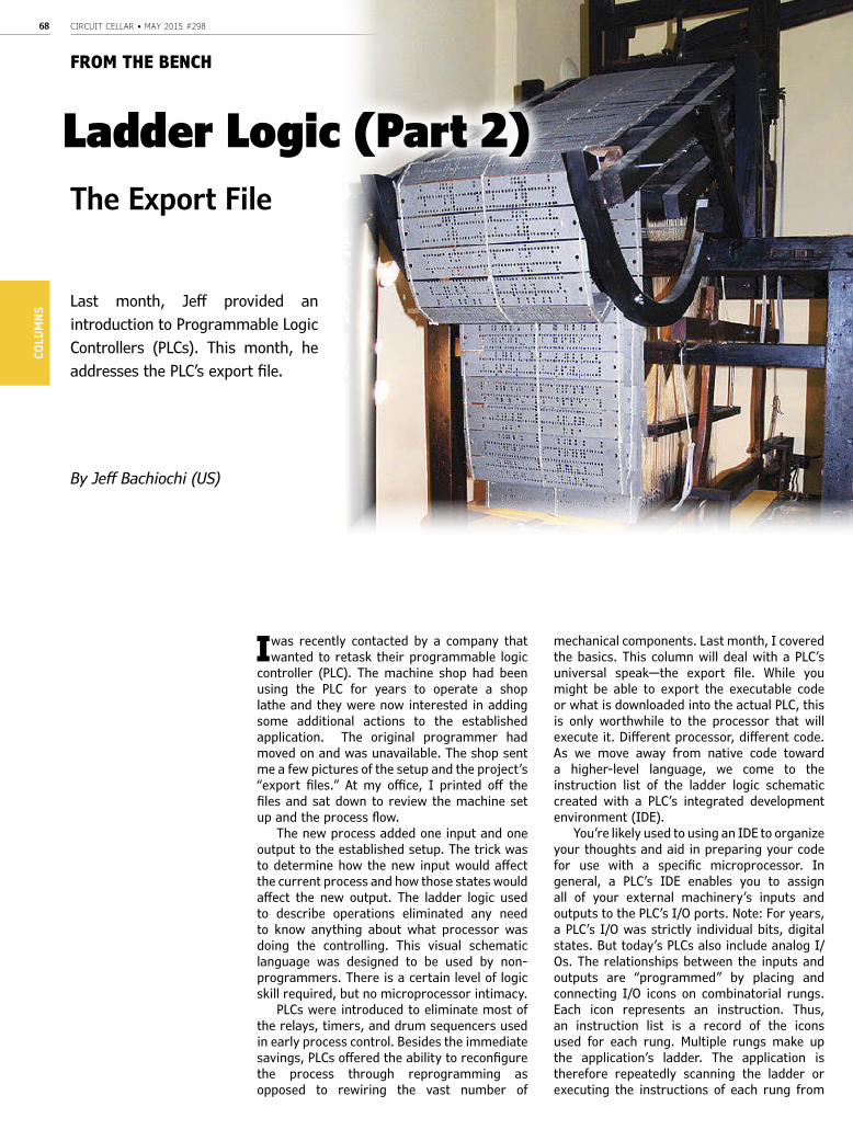
CIRCUIT CELLAR • MAY 2015 #29868CO
LUM
NS
I was recently contacted by a company that wanted to retask their programmable logic
controller (PLC). The machine shop had been using the PLC for years to operate a shop lathe and they were now interested in adding some additional actions to the established application. The original programmer had moved on and was unavailable. The shop sent me a few pictures of the setup and the project’s “export files.” At my office, I printed off the files and sat down to review the machine set up and the process flow.
The new process added one input and one output to the established setup. The trick was to determine how the new input would affect the current process and how those states would affect the new output. The ladder logic used to describe operations eliminated any need to know anything about what processor was doing the controlling. This visual schematic language was designed to be used by non-programmers. There is a certain level of logic skill required, but no microprocessor intimacy.
PLCs were introduced to eliminate most of the relays, timers, and drum sequencers used in early process control. Besides the immediate savings, PLCs offered the ability to reconfigure the process through reprogramming as opposed to rewiring the vast number of
mechanical components. Last month, I covered the basics. This column will deal with a PLC’s universal speak—the export file. While you might be able to export the executable code or what is downloaded into the actual PLC, this is only worthwhile to the processor that will execute it. Different processor, different code. As we move away from native code toward a higher-level language, we come to the instruction list of the ladder logic schematic created with a PLC’s integrated development environment (IDE).
You’re likely used to using an IDE to organize your thoughts and aid in preparing your code for use with a specific microprocessor. In general, a PLC’s IDE enables you to assign all of your external machinery’s inputs and outputs to the PLC’s I/O ports. Note: For years, a PLC’s I/O was strictly individual bits, digital states. But today’s PLCs also include analog I/Os. The relationships between the inputs and outputs are “programmed” by placing and connecting I/O icons on combinatorial rungs. Each icon represents an instruction. Thus, an instruction list is a record of the icons used for each rung. Multiple rungs make up the application’s ladder. The application is therefore repeatedly scanning the ladder or executing the instructions of each rung from
Ladder Logic (Part 2)
By Jeff Bachiochi (US)
Last month, Jeff provided an introduction to Programmable Logic Controllers (PLCs). This month, he addresses the PLC’s export file.
FROM THE BENCH
The Export File
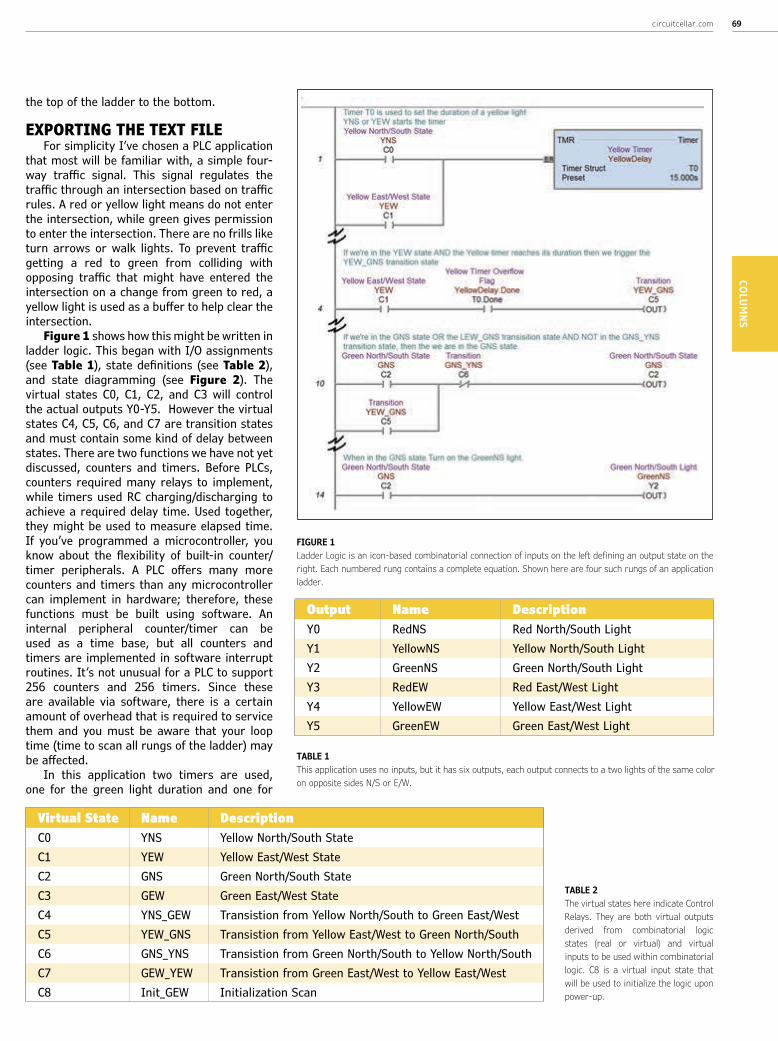
circuitcellar.com 69COLUM
NS
the top of the ladder to the bottom.
EXPORTING THE TEXT FILE For simplicity I’ve chosen a PLC application
that most will be familiar with, a simple four-way traffic signal. This signal regulates the traffic through an intersection based on traffic rules. A red or yellow light means do not enter the intersection, while green gives permission to enter the intersection. There are no frills like turn arrows or walk lights. To prevent traffic getting a red to green from colliding with opposing traffic that might have entered the intersection on a change from green to red, a yellow light is used as a buffer to help clear the intersection.
Figure 1 shows how this might be written in ladder logic. This began with I/O assignments (see Table 1), state definitions (see Table 2), and state diagramming (see Figure 2). The virtual states C0, C1, C2, and C3 will control the actual outputs Y0-Y5. However the virtual states C4, C5, C6, and C7 are transition states and must contain some kind of delay between states. There are two functions we have not yet discussed, counters and timers. Before PLCs, counters required many relays to implement, while timers used RC charging/discharging to achieve a required delay time. Used together, they might be used to measure elapsed time. If you’ve programmed a microcontroller, you know about the flexibility of built-in counter/timer peripherals. A PLC offers many more counters and timers than any microcontroller can implement in hardware; therefore, these functions must be built using software. An internal peripheral counter/timer can be used as a time base, but all counters and timers are implemented in software interrupt routines. It’s not unusual for a PLC to support 256 counters and 256 timers. Since these are available via software, there is a certain amount of overhead that is required to service them and you must be aware that your loop time (time to scan all rungs of the ladder) may be affected.
In this application two timers are used, one for the green light duration and one for
TABLE 1 This application uses no inputs, but it has six outputs, each output connects to a two lights of the same color on opposite sides N/S or E/W.
FIGURE 1Ladder Logic is an icon-based combinatorial connection of inputs on the left defining an output state on the right. Each numbered rung contains a complete equation. Shown here are four such rungs of an application ladder.
Output Name DescriptionY0 RedNS Red North/South LightY1 YellowNS Yellow North/South LightY2 GreenNS Green North/South LightY3 RedEW Red East/West LightY4 YellowEW Yellow East/West LightY5 GreenEW Green East/West Light
Virtual State Name DescriptionC0 YNS Yellow North/South StateC1 YEW Yellow East/West StateC2 GNS Green North/South StateC3 GEW Green East/West StateC4 YNS_GEW Transistion from Yellow North/South to Green East/WestC5 YEW_GNS Transistion from Yellow East/West to Green North/South C6 GNS_YNS Transistion from Green North/South to Yellow North/SouthC7 GEW_YEW Transistion from Green East/West to Yellow East/WestC8 Init_GEW Initialization Scan
TABLE 2The virtual states here indicate Control Relays. They are both virtual outputs derived from combinatorial logic states (real or virtual) and virtual inputs to be used within combinatorial logic. C8 is a virtual input state that will be used to initialize the logic upon power-up.
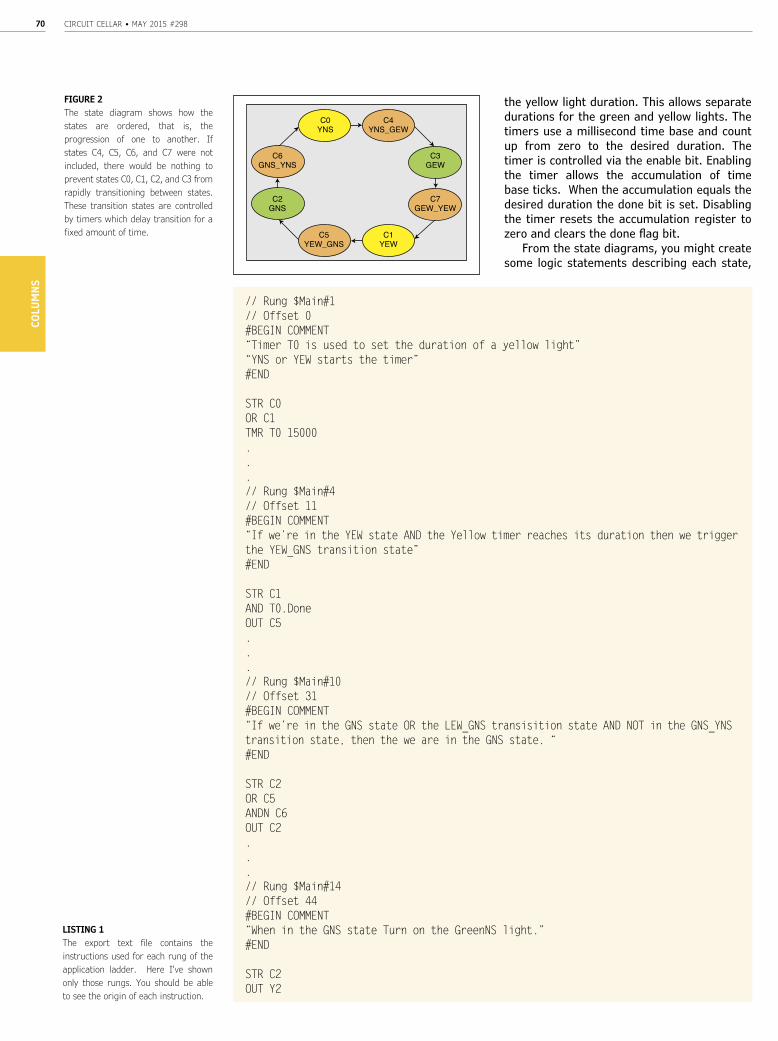
CIRCUIT CELLAR • MAY 2015 #29870CO
LUM
NS
the yellow light duration. This allows separate durations for the green and yellow lights. The timers use a millisecond time base and count up from zero to the desired duration. The timer is controlled via the enable bit. Enabling the timer allows the accumulation of time base ticks. When the accumulation equals the desired duration the done bit is set. Disabling the timer resets the accumulation register to zero and clears the done flag bit.
From the state diagrams, you might create some logic statements describing each state,
FIGURE 2The state diagram shows how the states are ordered, that is, the progression of one to another. If states C4, C5, C6, and C7 were not included, there would be nothing to prevent states C0, C1, C2, and C3 from rapidly transitioning between states. These transition states are controlled by timers which delay transition for a fixed amount of time.
C4YNS_GEW
C0YNS
C6GNS_YNS
C2GNS
C1YEW
C5YEW_GNS
C7GEW_YEW
C3GEW
LISTING 1The export text file contains the instructions used for each rung of the application ladder. Here I’ve shown only those rungs. You should be able to see the origin of each instruction.
// Rung $Main#1
// Offset 0
#BEGIN COMMENT
“Timer T0 is used to set the duration of a yellow light”
“YNS or YEW starts the timer”
#END
STR C0
OR C1
TMR T0 15000
.
.
.
// Rung $Main#4
// Offset 11
#BEGIN COMMENT
“If we’re in the YEW state AND the Yellow timer reaches its duration then we trigger
the YEW_GNS transition state”
#END
STR C1
AND T0.Done
OUT C5
.
.
.
// Rung $Main#10
// Offset 31
#BEGIN COMMENT
“If we’re in the GNS state OR the LEW_GNS transisition state AND NOT in the GNS_YNS
transition state, then the we are in the GNS state. “
#END
STR C2
OR C5
ANDN C6
OUT C2
.
.
.
// Rung $Main#14
// Offset 44
#BEGIN COMMENT
“When in the GNS state Turn on the GreenNS light.”
#END
STR C2
OUT Y2

circuitcellar.com 71COLUM
NS
but I‘ll skip this and go right to entering ladder logic which creates this visual image of these statements. If you refer back to Figure 1, you can see a rung from each section of the ladder following through a single transition process between the yellow light for the east/west traffic lanes and the green light for the north/south lanes. Let’s assume that the yellow east/west light is on, or True (C1=1). In the first rung, a true from either C0 or C1 will enable timer T0 and it will start counting. Execution continues with rungs 2, 3, and 4. In rung 4, C5 is False (C5=0), since even though C2 is True, T0 is not done yet T0.Done= False (both must be True). Rungs 5–10 execute, in rung 10 all are False so C2 must be False (C2=0). Rungs 11–14 execute and, again, if rung 14 C2 is off, output Y2 is off (Y2=0). Once all rungs have been evaluated, then outputs are written, inputs are read, and the ladder scan begins again with similar results until timer T0 reaches its 15-s duration. This time, when we hit rung 4, C1 and T0.Done are both True, so C5 is now True (C5=1). At rung 10, the C5 transition state is now True and the NOT state of C6 is True (NOT C6=0), so C2 is now True (C2=1). Note: In a similar rung to 10 (not shown), C1 was now found to be false, since even though it was True (at the start of the rung), C5 was now
FIGURE 3Here is the complete “Do More” PLC Instruction Set.
FrontPanelExpress.com
Cost effective prototypes and production runs with no setup charges
Powder-coated and anodized finishes in various colors
Select from aluminum, acrylic or provide your own material
Standard lead time in 5 days or express manufacturing in 3 or 1 days
You design it to your specifications using
our FREE CAD software, Front Panel Designer
We machine it and ship to you a
professionally finished product,no minimum quantity required
The Easiest Way to Design CustomFront Panels & Enclosures
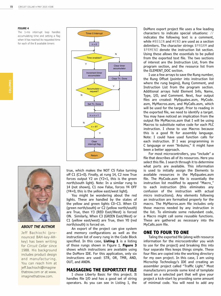
CIRCUIT CELLAR • MAY 2015 #29872CO
LUM
NS
true, which makes the NOT C5 False turning off C1 (C1=0). Finally, at rung 14, C2 now True forces output Y2 on (Y2=1, this is the green north/south light). Note: In a similar rung to 14 (not shown), C1 now False, forces Y4 OFF (Y4=0, this is the yellow east/west light).
You might be wondering about the red lights. These are handled by the states of the yellow and green lights C0–C3. When C0 (green north/south) or C2 (yellow north/south) are True, then Y3 (RED East/West) is forced ON. Similarly, When C3 (GREEN East/West) or C1 (yellow east/west) are True, then Y0 (red north/south) is forced on.
An export of the project can give system and memory configurations as well as the instruction list of every rung in the Code Block specified. In this case, Listing 1 is a listing of those rungs shown in Figure 1. Figure 3 shows which instructions are available using the DoMore IDE. For this application, only six instructions are used: STR, OR, TMR, AND, OUT, and ANDN.
MASSAGING THE EXPORT.TXT FILEI chose Liberty Basic for this project. It
handles file I/O and has a good set of string operators. As you can see in Listing 1, the
DoMore export project file uses a few leading characters to indicate special situations: // indicates the following text is a comment, while #BEGIN and #END are used as a section delimiters. The character strings $PRGRM and $PRMEND denote the instruction list section. Using these allows the essentials to be pulled from the exported text file. The two sections of interest are the Instruction List, from the program section, and the resource list from the ELEMENT_DOC section.
I use a few arrays to save the Rung number, the Rung Offset (pointer into instruction list where the rung begins), Rung Comment, and Instruction List from the program section. Additional arrays hold Element Info, Name, Type, I/O, and Comment. Next, four output files are created: MyEquates.asm, MyCode.asm, MyMacros.asm, and MyCalls.asm, which will be used for the target. Prior to reading in the exported file, we need to identify a target. You may have noticed an implication from the output file MyMacros.asm that I will be using Macros to substitute native code for each PLC instruction. I chose to use Macros because this is a good fit for assembly language. Note: I could have used function calls for each instruction. If I was programming in C language or even “Arduino,” it might have been a better approach.
For most microcontrollers, you “include” a file that describes all of its resources. Here you select this file. I search through it to determine what ports are available. This information is used to initially assign the Elements to available resources in the MyEquates.asm file. The MyCode.asm file is essentially the instruction list modified to append “Macro_” to each instruction (this eliminates any confusion of the instruction with actual micro instructions). Any elements following an instruction are formatted properly for the macro. The MyMacros.asm file includes only those macros needed by any instruction in the list. To eliminate some redundant code, a Macro might call some reusable functions. These are gathered as necessary into the MyCalls.asm file.
ONE TO FOUR TO ONETaling the exported file (along with resource
information for the microcontroller you wish to use for the project) and breaking this into four separate files keeps things simple. These four files are copied into the working directory for my own project. In this case, I am using Microchip Technology’s IDE and creating an assembler project called “Traffic Light.” Most manufacturers provide some kind of template based on a selected part that will give your project a kick-start by providing some amount of minimal code. You will need to add any
FIGURE 4The 1-ms interrupt loop handles accumulating time and setting a flag when it has reached its requested time for each of the 8 available timers
Timer 0 Interrupt
Time enabled?
Clear timeraccumulator
Increment timeraccumulator
Clear Tn. Done
Accumulator <request?
Set Tn. Done
n = n + 1
n = 8?
Clearinterrupt flag
Y
Y
N
N
n = 0
Y
N
Return
ABOUT THE AUTHORJe f f Bachioch i (pro-nounced BAH-key-AH-key) has been writing for Circuit Cellar since 1988. His background includes product design and manufac tur ing . You can reach him at jeff.bachiochi@imagine thatnow.com or at www.imaginethatnow.com.

If you’ve ever wanted to design and program with the ADuC841 microcontroller, or other microcontrollers in the 8051 family, this is the book
for you. With introductory and advanced labs, you’ll soon master the many ways to use a microcontroller. Perfect for academics!
Now Just $35.00
If you’ve ever wanted to design and program with the ADuC841
ADuC841 Microcontroller Design Manual:From Microcontroller Theory to Design Projects
www.cc-webshop.com Buy it today!

CIRCUIT CELLAR • MAY 2015 #29874CO
LUM
NS
constants you might need in your application, like identifying some flag bits or timer reload values. In addition, I defined some default values for all of the port registers such that they default to all digital inputs. I defined a number of variables, especially the PLC working registers. This area is defined for 128 inputs (Xn), 128 outputs (Yn), 128 Control Relays (Cn), eight timer enable bits (Tn), eight timer done flag bits (Tn.Done), eight counter enable bits, eight counter done flag bits (CNTn), 128 system flag bits (CNTn.Done), and eight Master Lines. Each timer and counter also has a 32-bit accumulator and 32-bit request register. The MyEquates.asm file uses labels found here to determine its reference. For instance, the Element “Y0” is assigned to the first output bit.
When an application begins, there are some things that must be initialized. In particular each port must be defined as input or output and in some instances an analog or digital input. Earlier I discussed creating some default values for all ports. If the MyEquates.asm is included after the constants have been defined, then it can redefine any ports it needs to change. In this case, no physical inputs are used—only 6 physical outputs. MyEquate.asm redefines TRISA (PORTA direction register) as B’11000000’, the first 6 bits as outputs. Any peripherals required must be set up here as well. Timers are required in this application. MyMacro.asm has already been some support code for the TMR (macro). This code handles enabling/disabling any timer (Tn) and checking the timer done flags (Tn.Done). However, we need to provide the background function for eight timers based on the counter timer peripheral available. This is handled by a timer interrupt routine in this framework. Timer0 is set up to interrupt every 1 ms. Refer to Figure 4 for a flow chart of the code loop used for the eight software timers.
As I discussed earlier, a PLC scan is based on three phases: read physical inputs, scans each rung of the ladder to determine end-of-rung states, and write physical outputs. This loop is endless and becomes the Main loop. I just mentioned initializing the microcontroller, but I must also initialize the application state. With all states OFF, all rungs will equate to an OFF state and “nothing” will keep happening forever. To kick-start the application, you need to initialize a state as ON. This is where the Main.FirstScan flag comes into play. This is a system flag that can be used to cause something to happen once during the first scan of the ladder. It is set to ON (“1”) until the ladder has been scanned once and then it is cleared (“0”). To handle this and other system tasks, a fourth
circuitcellar.com/ccmaterials
RESOURCEPLCopen, “IEC 61131-3: A Standard Programming Re-source,” www.plcopen.org/pages/tc1_standards/down-loads/intro_iec.pdf.
SOURCESDo-more Designer Windows-based program-ming softwareAutomation Direct | www.automationdirect.com MPLAB IDE and PIC18F18K50 Microcontroller Microchip Technology | www.microchip.com
Liberty BasicShoptalk Systems | www.libertybasic.com
LISTING 2To emulate a PLC in a microcontroller, four functions are required in the Main CodeLoop. System actions are those that might be required outside of the normal ladder loop, like a one time event requested by a user. The ladder loop consists of reading the physical inputs into system variables, evaluating each ladder rung, and setting physical output states based on system variables.
Main_CodeLoop
call SystemActions
;
call ReadInputs
;
#INCLUDE <MyCode.asm>
;
call WriteOutputs
;
goto Main_CodeLoop
PHOTO 1 This plastic model randomly blinked a red, yellow, and green 7.5-W Christmas tree lights until I ripped out the guts and replaced them with individual white LEDs for each colored lens. The exported ladder logic instruction list was converted into PIC code using macro language substitution. The PIC operates as a PLC controlling the traffic light pattern.
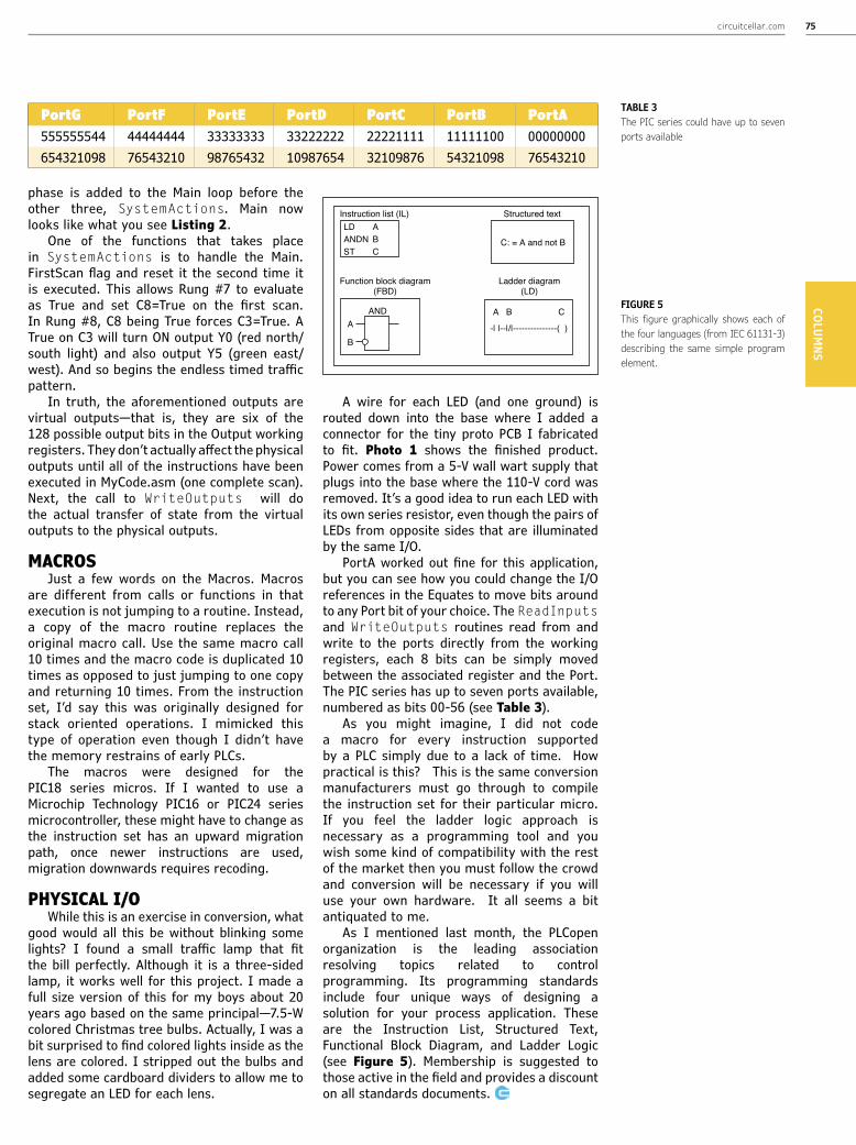
circuitcellar.com 75COLUM
NS
phase is added to the Main loop before the other three, SystemActions. Main now looks like what you see Listing 2.
One of the functions that takes place in SystemActions is to handle the Main.FirstScan flag and reset it the second time it is executed. This allows Rung #7 to evaluate as True and set C8=True on the first scan. In Rung #8, C8 being True forces C3=True. A True on C3 will turn ON output Y0 (red north/south light) and also output Y5 (green east/west). And so begins the endless timed traffic pattern.
In truth, the aforementioned outputs are virtual outputs—that is, they are six of the 128 possible output bits in the Output working registers. They don’t actually affect the physical outputs until all of the instructions have been executed in MyCode.asm (one complete scan). Next, the call to WriteOutputs will do the actual transfer of state from the virtual outputs to the physical outputs.
MACROSJust a few words on the Macros. Macros
are different from calls or functions in that execution is not jumping to a routine. Instead, a copy of the macro routine replaces the original macro call. Use the same macro call 10 times and the macro code is duplicated 10 times as opposed to just jumping to one copy and returning 10 times. From the instruction set, I’d say this was originally designed for stack oriented operations. I mimicked this type of operation even though I didn’t have the memory restrains of early PLCs.
The macros were designed for the PIC18 series micros. If I wanted to use a Microchip Technology PIC16 or PIC24 series microcontroller, these might have to change as the instruction set has an upward migration path, once newer instructions are used, migration downwards requires recoding.
PHYSICAL I/OWhile this is an exercise in conversion, what
good would all this be without blinking some lights? I found a small traffic lamp that fit the bill perfectly. Although it is a three-sided lamp, it works well for this project. I made a full size version of this for my boys about 20 years ago based on the same principal—7.5-W colored Christmas tree bulbs. Actually, I was a bit surprised to find colored lights inside as the lens are colored. I stripped out the bulbs and added some cardboard dividers to allow me to segregate an LED for each lens.
A wire for each LED (and one ground) is routed down into the base where I added a connector for the tiny proto PCB I fabricated to fit. Photo 1 shows the finished product. Power comes from a 5-V wall wart supply that plugs into the base where the 110-V cord was removed. It’s a good idea to run each LED with its own series resistor, even though the pairs of LEDs from opposite sides that are illuminated by the same I/O.
PortA worked out fine for this application, but you can see how you could change the I/O references in the Equates to move bits around to any Port bit of your choice. The ReadInputs and WriteOutputs routines read from and write to the ports directly from the working registers, each 8 bits can be simply moved between the associated register and the Port. The PIC series has up to seven ports available, numbered as bits 00-56 (see Table 3).
As you might imagine, I did not code a macro for every instruction supported by a PLC simply due to a lack of time. How practical is this? This is the same conversion manufacturers must go through to compile the instruction set for their particular micro. If you feel the ladder logic approach is necessary as a programming tool and you wish some kind of compatibility with the rest of the market then you must follow the crowd and conversion will be necessary if you will use your own hardware. It all seems a bit antiquated to me.
As I mentioned last month, the PLCopen organization is the leading association resolving topics related to control programming. Its programming standards include four unique ways of designing a solution for your process application. These are the Instruction List, Structured Text, Functional Block Diagram, and Ladder Logic (see Figure 5). Membership is suggested to those active in the field and provides a discount on all standards documents.
FIGURE 5 This figure graphically shows each of the four languages (from IEC 61131-3) describing the same simple program element.
Instruction list (IL)
Function block diagram(FBD)
Ladder diagram(LD)
A B C
Structured text
C: = A and not B
A
B
LD AANDN BST C
AND
-| |--|/|---------------( )
PortG PortF PortE PortD PortC PortB PortA555555544 44444444 33333333 33222222 22221111 11111100 00000000654321098 76543210 98765432 10987654 32109876 54321098 76543210
TABLE 3 The PIC series could have up to seven ports available

CIRCUIT CELLAR • MAY 2015 #29876
CC SHOP
1
4
3
Further information and ordering: www.cc-webshop.comCONTACT US: Circuit Cellar, Inc. | Phone: 860.289.0800 | E-mail: [email protected]
2
2 ADVANCED CONTROL ROBOTICSWhen it comes to robotics, the future is now! This book simplifies the
theory and best practices of advanced robot technologies by providing insight to communication technologies, control robotics, embedded technology, programming, and more. Complete with code samples, schematics, and design tips. Great reading for beginners and experts alike.
Author: Hanno SanderItem#BK-ELNL-978-0-963013-33-0
4 CC VAULTCC Vault is a pocket-sized USB that comes fully loaded with every
issue of Circuit Cellar magazine! This comprehensive archive provides an unparalleled amount of embedded hardware and software design tips, schematics, and source code. CC Vault contains all the trade secrets you need to become a better, more educated electronics engineer!
Item #: CCVAULT
3 CC 2014 CD2014 was an exciting year for electronics engineers! The continued
success of open-source solutions, Internet of Things (IoT) revolutions, and green-energy consciousness has changed the face of embedded design indefinitely. In Circuit Cellar’s 2014 archive CD, you can find all of these hot topics and gain insight into how experts, as well as your peers, are putting the newest technologies to the test. You’ll have access to all articles, schematics, and source code published from January to December 2014.
Item #: CD-018-CC2014
Previous Years Also Available
1 CC 2014 DIGITAL ARCHIVE SUBSCRIPTIONJust when you thought it couldn’t get any easier than a thumb
drive...you can now access a full year of Circuit Cellar from any device connected to the Internet! (2014: 12 issues)
You get all the benefits of a printed copy—bookmark pages, make annotations, and write in the margins—combined with the digital advantages of easy storage, zoom, links, and search features.
Item #: CC-DA-2014

circuitcellar.com 77TESTS &
CHALLENGES
TEST YOUR EQ Contributed by David Tweed
What’s your EQ? The answers are posted at www.circuitcellar.com/category/ test-your-eq/. You can contact the quizmasters [email protected].
PROBLEM 1—What do we call a network of gates that has no feedback of any kind? What is its key characteristic?
PROBLEM 2—What do we call a network of gates that has negative feedback? Give an example.
PROBLEM 3—What do we call a network of gates that has positive feedback? Give an example of the simplest possible such network (there are several).
PROBLEM 4—Why are NAND gates and NOR gates considered to be “universal” gates? Why is this important?
You’ll receive electrical engineering tips, interesting electronics projects, embedded systems industry news, and exclusive product deals via e-mail to your inbox on a regular basis. If you’re looking for essential electrical engineering-related information, we’ve got you covered: micrcontroller-based projects, embedded development, programmable logic, wireless communications, robotics, analog techniques, embedded programming, and more!
Subscribe now to stay up-to-date with our latest content, news, and offers!
Sign up for the
FREE Circuit Cellar Newsletter!
circuitcellar.com

CIRCUIT CELLAR • MAY 2015 #29878TE
STS
& C
HALL
ENGE
S
ACROSS1. 10-18 of a second3. A barrier of conductive or magnetic matter4. Relating to touch6. Signal processing for sensor arrays8. A sequence, instructions10. A small potentiometer used for making preset
adjustments in a circuit12. Light intensity14. Degauss17. Xe18. Sharing the same axis19. 0.1 bel
CROSSWORD The answers will be available at circuitcellar.com/category/crossword/
MAY 2015
1 2
3
4 5 6 7
8 9
10 11
12 13
14 15
16 17
18
19
EclipseCrossword.com
DOWN2. 0.3937 inches5. Flexible sharp wire that connects to a semiconductor
crystal’s surface [two words]7. 0.0000000000000018. Less than 15 Hz9. An abrupt burst of signal energy11. Mechanically driven generator of AC electricity13. DIY, homemade15. Current flow over time16. 200 bits per second = 200 what?

circuitcellar.com 79the directory ofPRODUCTS & SERVICES
For current rates, deadlines, and more information contact Peter Wostrel at 978.281.7708 or [email protected].
IDEA BOX
microEngineering Labs, Inc.www.melabs.com 888-316-1753
PIC is a registered trademark of Microchip Technology Inc. in the USA and other countries.
Programmers for Microchip PIC® Microcontrollers
PC-Tethered USB Model (shown):
Stand-Alone Field Programmer:
Program in-circuit or use adapters for unmounted chips.
Zero-Insertion-Force Adapters available for DIP, SOIC, SSOP, TQFP, and more.
Starting at $79.95
$20 for 5PCBs 2 layer,4x4inch, FR4(RoHS),0.063”,1oz,
2LPI,Green,1SK,Lead free HASL
Standard PCB: Promotion code:
CC14061
PCB & PCBA Small to Mass QTY
INSTANT QUOTE AT:
www.myropcb.comOR CALL:
1-888-PCB-MYRO
262-522-6500 x 35
PIC® MCU is a registered trademark of Microchip Technology Inc.
www.ccsinfo.com/CC515Download Free Evaluation:
EZ APP LYNX
Bluetooth® word mark and logos are registered trademarks owned by Bluetooth SIG, Inc.
Library to Interface a PIC® to Smartphones & Tablets with Bluetooth®
NEW GUI & Style Components:
Status/Gas Gauges, Buttons,
Sliders, Text Sizes, Colors,
Margins & more...
No APP Programming!
Free generic App works with library included with IDE C Compilers
Create a wireless sensor or
controller on a PIC® for Android™!
Android is a trademark of Google Inc.
CIRCUIT CELLAR • MAY 2015 #29880TE
CH T
HE F
UTUR
E
Robots have been around for over half a century now, making constant progress in
terms of their sophistication and intelligence levels, as well as their conceptual and literal closeness to humans. As they become smarter and more aware, it becomes easier to get closer to them both socially and physically. That leads to a world where robots do things not only for us but also with us.
Not-so-intelligent robots made their first debut in factory environments in the late ‘50s. Their main role was to merely handle the tasks that humans were either not very good at or that were dangerous for them. Traditio-nally, these robots have had very limited sen-sing; they have essentially been blind despite being extremely strong, fast, and repeatable. Considering what consequences were likely to follow if humans were to freely wander about within the close vicinity of these strong, fast, and blind robots, it seemed to be a good idea to isolate them from the environment by pla-cing them in safety cages.
Advances in the fields of sensing and com-pliant control made it possible to get a bit closer to these robots, again both socially and physically. Researchers have started propo-sing frameworks that would enable human-robot collaborative manipulation and task execution in various scenarios. Bi-manual collaborative manufacturing robots like YuMi by ABB and service robots like HERB by the Personal Robotics Lab of Carnegie Mellon University[1] have started emerging. Various modalities of learning from/programming by demonstration, such as kinesthetic teaching and imitation, make it very natural to interact with these robots and teach them the skills and tasks we want them perform the way we teach a child. For instance, the Baxter robot by Rethink Robotics heavily utilizes these capabilities and technologies to potentially bring a teachable robot to every small com-pany with basic manufacturing needs.
As robots gets smarter, more aware, and safer, it becomes easier to socially accept and trust them as well. This reduces the physical distance between humans and robots even further, leading to assistive robotic technolo-gies, which literally “live” side by side with humans 24/7. One such project is the Assis-tive Dexterous Arm (ADA)[2] that we have been carrying out at the Robotics Institute and the Human-Computer Interaction Institute of Carnegie Mellon University. ADA is a wheel-chair mountable, semi-autonomous manipu-lator arm that utilizes the sliding autonomy
concept in assisting people with disabilities in performing their activities of daily living. Our current focus is on assistive feeding, where the robot is expected to help the users eat their meals in a very natural and socially ac-ceptable manner. This requires the ability to predict the user’s behaviors and intentions as well as spatial and social awareness to avoid awkward situations in social eating settings. Also, safety becomes our utmost concern as the robot has to be very close to the user’s face and mouth during task execution.
In addition to assistive manipulators, there have also been giant leaps in the research and development of smart and lightweight exoskeletons that make it possible for para-plegics to walk by themselves. These exoske-letons make use of the same set of techno-logies, such as compliant control, situational awareness through precise sensing, and even learning from demonstration to capture the walking patterns of a healthy individual.
These technologies combined with the recent developments in neuroscience have made it possible to get even closer to humans than an assistive manipulator or an exoskele-ton, and literally unite with them through in-telligent prosthetics. An intelligent prosthetic limb uses learning algorithms to map the re-ceived neural signals to the user’s intentions as the user’s brain is constantly adapting to the artificial limb. It also needs to be highly compliant to be able to handle the vast vari-ance and uncertainty in the real world, not to mention safety.
Extrapolating from the aforementioned de-velopments and many others, we can easily say that robots are going to be woven into our lives. Laser technology used to be unre-achable and cutting-edge from an average person’s perspective a couple decades ago. However, as Rodney Brooks says in his book titled Robot: The Future of Flesh and Machi-nes, (Penguin Books, 2003), now we do not know exactly how many laser devices we have in our houses, and more importantly we don’t even care! That will be the case for the robots. In the not so distant future, we will be en-joying the ride in our autonomous vehicle as a bunch of nanobots in our blood stream are delivering drugs and fixing problems, and we will feel good knowing that our older relatives are getting some great care from their assis-tive companion robots.
The Future of Intelligent Robots
[1] http://www.cmu.edu/herb-robot/[2] https://youtu.be/glpCAdKEWAA
By Tekin Meriçli
Tekin Meriçli, PhD, is a well-rounded roboticist with in-depth expertise in machine intelligence and learning, perception, and manipulation. He is currently a Postdoctoral Fellow at the Human-Computer Interaction Institute at Carnegie Mellon University, where he leads the efforts on building intuitive and expressive interfaces to interact with semi-autonomous robotic systems that are intended to assist elderly and disabled. Previously, he was a Postdoctoral Fellow at the National Robotics Engineering Center (NREC) and the Personal Robotics Lab of the Robotics Institute at Carnegie Mellon University. He received his PhD in Computer Science from Bogazici University, Turkey.

CC Vault
Unlock the power of embedded design.
Order yours today! cc-webshop.com*CC Vault is a 16-GB USB drive.
A vault of need-to-know information in the fields of embeddedhardware, embedded software, and computer applications
This pocket-sized vault comes fully loaded with every issue of Circuit Cellar magazine and serves as an unparalleled resource for embedded hardware and software design tips, schematics, and source code.
From green energy design to ‘Net-enabled devices, maximizing power to minimizing footprint, CC Vault* contains all the trade secrets you need to become a better, more educated electronics engineer.

We bring the full range of Electronic Contract
Manufacturing services to your fingertip!
This is the only place where you would put all
your eggs in one basket to get fastest time to
market. From concept design to prototype to
full turnkey production on all your
electronic products.
ENCLOSURES
KEYPADSASSEMBLY
FABRICATION
www.PCBnet.com
847-806-0003 [email protected]
Certified Woman-Owned Small Business
Imagineering
WinnerFamily Entrepreneurship
Award 2014