exploration and exploitation with insufficient resources

JMLR: Workshop and Conference Proceedings vol 26 (2012) 37–61 On-line Trading of Exploration and Exploitation 2

Exploration and Exploitation with Insufficient Resources

Chris Lovell [email protected]

Gareth Jones [email protected]

Klaus-Peter Zauner [email protected]

Steve R. Gunn [email protected]

School of Electronics and Computer Science,

University of Southampton, UK

Editor: Dorota G lowacka, Louis Dorard and John Shawe-Taylor

Abstract

In physical experimentation, the resources available to discover new knowledge are typicallyextremely small in comparison to the size and dimensionality of the parameter spaces thatcan be searched. Additionally, due to the nature of physical experimentation, experimentalerrors will occur, particularly in biochemical experimentation where the reactants mayundetectably denature, or reactant contamination could occur or equipment failure. Theseerrors mean that not all experimental measurements and observations will be accurateor representative of the system being investigated. As the validity of observations is notguaranteed, resources must be split between exploration to discover new knowledge andexploitation to test the validity of the new knowledge. Currently we are investigatingthe automation of discovery in physical experimentation, with the aim of producing afully autonomous closed-loop robotic machine capable of autonomous experimentation.This machine will build and evaluate hypotheses, determine experiments to perform andthen perform them on an automated lab-on-chip experimentation platform for biochemicalresponse characterisation. In the present work we examine how the trade-off betweenexploration and exploitation can occur in a situation where the number of experiments thatcan be performed is extremely small and where the observations returned are sometimeserroneous or unrepresentative of the behaviour being examined. To manage this trade-offwe consider the use of a Bayesian notion of surprise, which is used to perform explorationexperiments whilst observations are unsurprising from the predictions that can be madeand exploits when observations are surprising as they do not match the predicted response.

Keywords: Limited resources, exploration–exploitation, Bayesian surprise

1. Introduction

In physical experimentation, the resources typically available are generally small in com-parison to the size and scale of the parameter space. For example there may perhaps beonly a handful of experiments available per parameter dimension. In general the amount ofresources can be considered as being ‘not enough’ to provide a highly confident predictionof the behaviour being observed. Therefore the goal is to get a good reliable prediction ofthe observable behaviours, with as few experiments as possible. To aid the experimenter,statistical machine learning techniques can be employed to perform pattern analysis on thedata available and choose the experiments to perform, with the goal of maximising theinformation gained whilst minimising the resources spent. These techniques are similar

c© 2012 C. Lovell, G. Jones, K.-P. Zauner & S.R. Gunn.

Lovell Jones Zauner Gunn

Hypothesis Manager

Experiment Manager

Observations

Artificial Experimenter Experimentation Platform

parameters

Figure 1: Overview of an artificial experimenter combined with an automated experimen-tation platform to allow for autonomous experimentation. The artificial experi-menter uses the information available to build hypotheses and determine experi-ments to perform. It provides experiment parameters to perform and is providedthe observational results for those experiments. Also shown is a fully automatedlab-on-chip based experimentation platform under development. The syringeson the right of the device hold the liquid reactants available. The flow of re-actants is controlled by on-chip valves driven by computer controlled solenoids.The platform contains a UV photometer that allows for measurements of opticalabsorbance to be taken for reactants flowing within the microfluidic chip. Themeasurements are the observations returned.

to computational scientific discovery (Langley et al., 1987) and active learning (MacKay,1992; Cohn et al., 1994; Settles, 2009). We label the combination of techniques that areimplemented to perform this pattern recognition and adaptive experiment selection withina laboratory problem, as an artificial experimenter (Lovell et al., 2010). When combinedwith automated hardware capable of performing the experiments requested, an autonomousexperimentation machine can be created as illustrated in Figure 1.

Additionally to the limited resources problem, physical experimentation has the problemthat experimental errors or unexpected undetectable physical changes in the reactants canoccur, which can yield observations not representative of the behaviour being investigated.These erroneous observations can be thought of as being outliers, except that there willbe insufficient data available to identify them as such with any degree of confidence. Oneapproach to handling this uncertainty in the observation validity, is to consider multiplehypotheses in parallel that have different views about the data (Lovell et al., 2010). Theinformation within these hypotheses can be exploited to select experiments where theymost disagree, in order to obtain experiments that can dismiss invalid hypotheses. Howeverexperiments must also be performed that can search for features of the behaviour that havenot yet been characterised. The artificial experimenter has to make a continual trade-off

38


between performing experiments to discover features of the behaviour not yet identified, withspending resources to ensure that the current models of the behaviour being investigatedare accurate. With too little exploration, features of the behaviour such as local maximaand minima will be missed, resulting in poor scope of the hypotheses. Whilst with too littleexploitation, inaccuracies and errors will occur in the hypotheses caused by the erroneousobservations, resulting in hypotheses with poor accuracy.

We argue that in a situation where the resources are extremely limited and the obser-vations may not always be representative of the true underlying behaviour, an experimentselection strategy will want to disprove invalid hypotheses when there is disagreement aboutthe behaviour or validity of an observation and search for new discoveries when they agree.In other words, exploit the information held within the hypotheses to select experimentsthat maximise the discrimination between the hypotheses when there are good hypothe-ses supported by the experimental evidence that disagree. Whilst exploring the parameterspace when there is no disagreement between good hypotheses. To manage this trade-off weuse a Bayesian formulation of surprise, first used to identify surprising occurrences in videosequences (Itti and Baldi, 2009). In this work, the surprise is used such that exploitationoccurs when the previous experiment was surprising and exploration occurs when the previ-ous experiment was not surprising. The use of surprise to manage this trade-off is analogousto techniques performed by successful human scientists, who will perform focussed experi-ments to learn why an experiment yielded a surprising or unexpected observation (Kulkarniand Simon, 1990).

Here we discuss how the trade-off between exploration and exploitation has been consid-ered within an artificial experimenter that can perform automatic response characterisationwith a small, noisy and potentially erroneous set of observations. In particular enzymaticresponses has been considered as the domain to evaluate the techniques, however the designof the artificial experimenter is domain independent. As current active learning techniquesdo not fully capture the problems and uncertainties faced in physical experimentation, wetake the approach of addressing the problem and filling the gaps through attempting to cap-ture how successful scientists operate and make decisions, which make the techniques formanaging the trade-off presented here driven more from practise than theory. In Section 2we briefly re-pose the problem within a multi-armed bandit framework. In Section 3 webriefly discuss how hypotheses are represented within the system. In Section 4 we discussdifferent methods that have been used for managing the exploration–exploitation trade-offwithin our artificial experimenter. These techniques are evaluated through a 1-dimensionalsimulated trial and laboratory trial in Section 5, along with a 2-dimensional simulated trialin Section 6. In Section 7 we discuss how previous systems have addressed the exploration–exploitation trade-off.

2. Description of the Problem within a Multi-Armed Bandit Framework

For ease of understanding the present problem within the exploration-exploitation com-munity, we abstract the problem to one within a multi-armed bandit framework. In themulti-armed bandit problem there are a number of levers, which correspond to differentpossible experiments, which when pulled return some reward. The reward obtained inexperimentation is not directly a monetary reward, but rather an information reward. As-

39


suming we have multiple hypotheses in consideration and that we take the philosophy ofscience view that information is obtained by disproving hypotheses (Chamberlin, 1890), anexample of a rewarding experiment would be one that will provide information to discrimi-nate between a number of good hypotheses. A prediction of the minimum expected rewardcan be made by examining the current hypotheses under consideration and determining thedifference in predictions for them across the possible experiment parameters. However theactual reward may be much higher than predicted in regions where few experiments havebeen performed and where the predictions of the hypotheses are not representative of thetrue behaviour being investigated. Selecting where the hypotheses are maximally differentwill therefore be equivalent to exploitation. The goal therefore for experimentation is thesame as a multi-armed bandit problem, to maximise the reward, or information obtained,over a number of trials or experiments. However not all experiments will produce a reward,take for example the case where all hypotheses agree with the observation obtained and nonew information is learnt. Additionally the number of experiments that can be afforded willbe many times smaller than the total number of unique experiment parameters or levers.Furthermore the reward available on a particular experiment will generally reduce over time,as the hypotheses under consideration become more accurate in predicting the outcome ofan experiment. Although there will be cases where the reward available on a particularexperiment may increase over the previous experiment, for example where an erroneousobservation occurs that seemingly provides information to disprove a large number of goodhypotheses. In cases where a large information gain has occurred, repeat experiments maybe useful to determine the validity of an observation, however multiple repeats will leadto a reward tending towards zero. Therefore it is clear that the reward actually obtainedby pulling a lever or performing an experiment, would not be modelled by a single staticnormal distribution within a multi-armed bandit abstraction, but by a distribution wherethe mean alters over time and there are perhaps two variances, one small variance thatprovides experimental noise on all experiments, with a second larger variance that pro-vides erroneous observations to some experiments. Due to the differing rewards availableover time, the regret function will be similar to that used by Auer (2002), to compare themaximum reward available at time t with the actual reward obtained:

ρ =T∑t=1

(maxx∈X{It(x)} − it

)(1)

where maxx∈X {It(x)} is the maximum reward possible at time t, X is the set of possibleexperiments, and it is the actual reward at time t. Although due to the resource limitationan upper confidence bound approach will not be suitable as it will be unable to initialisethe predicted means.

3. Predicting the Behaviour Under Investigation

The present problem of response characterisation can be clearly addressed through usinga regression technique. Here spline based regression techniques form the foundation of thehypothesis representation, although alternate techniques could be substituted. Specifically,the techniques used are the smoothing spline in the 1-dimensional problem and thin platesplines in higher dimensions (Wahba, 1990). However, a single hypothesis or distribution

40


will perform poorly in situations where there are limited observations, with the validity ofthose observations not guaranteed (Lovell et al., 2010). The poor performance is due to thesingle hypothesis having to decide on the validity of observations. With little experimentaldata available, the technique may not be able to correctly identify an outlying observationthat is erroneous, causing it to overfit to the error. Alternatively the opposite could oc-cur, where a parameter selection technique like cross-validation may incorrectly identify anapparent outlying observation and ignore it, even though the observation is representativeof the behaviour being investigated and it is the hypothesis that it incorrect. Instead weconsider the use of multiple hypotheses, similar to query-by-committee (Seung et al., 1992).The multiple hypotheses are used to provide different views about the data that can beconsidered in parallel, with decisions made about which was the correct decision when moredata becomes available. Additionally the multiple hypotheses can be used later in experi-ment selection, to provide a method for exploitation through selecting where the hypotheseswith the most supporting experimental evidence disagree the most.

To deal with the uncertainty caused by only having a limited number of noisy and po-tentially erroneous observations, a hypothesis manager is used to consider many hypothesesin parallel (Lovell et al., 2010). Each hypothesis can maintain a different view of the be-haviour being investigated, along with different views about the validity of observations.In our design, hypotheses go through a process of refinement in cases where observationsdo not agree with hypotheses, to develop hypotheses that should be more representativeof the true underlying behaviour. An observation and hypothesis are identified as beingin disagreement when the observation falls outside of the 95% error bar interval for theprediction of the hypothesis. When refining a hypothesis under these circumstances, thesystem must take into consideration the problem that it will not know whether the dis-agreement between observation and hypothesis is because the hypothesis is incorrect, or ifthe observation is erroneous. The refinement process handles this consideration by creatingtwo new refinements of the original hypothesis that the observation disagreed with. In onerefinement the disagreeing observation will be declared to be erroneous and the observa-tion will receive a weight of 0, with all other parameters remaining the same. In the otherrefinement, the observation will be declared to be valid and the observation will be givena high weight, with all other parameters remaining the same. The zero weight will causethe regression to ignore the observation, whilst a high weight will draw the output of theregression curve closer to the observation. The original and two refined hypotheses are allkept in consideration by the hypothesis manager within a working set of hypotheses.

After each experiment is performed, the hypothesis manager creates a new set of hy-potheses with random initial parameters to give different starting views of the behaviourbeing investigated. These hypotheses are added to the working set of hypotheses that werekept in consideration in previous rounds of experimentation. All hypotheses are then com-pared to all observations to identify any disagreements, where refinements are made to thehypotheses in cases where there are disagreements. Finally all hypotheses are evaluatedagainst all of the previous observations to determine their confidence and quality. By main-taining a working set, or committee of different hypotheses, decisions about the shape ofthe response or validity of observations can be postponed until sufficient data is availableto reject incorrect assumptions. For computational performance, a number of the worstperforming hypotheses can be removed.

41


4. Experiment Selection

The experiment manager determines the experiments to perform using the informationavailable within the hypotheses along with information about where in the parameter spaceprevious experiments have been performed. In choosing experiments, the experiment man-ager needs to ensure that the parameter space is explored to allow for the discovery of newfeatures of the behaviour being investigated, whilst also making sure that data is obtainedthat can differentiate between the different hypotheses under consideration to identify themost likely candidate. We do not consider the case where the experiment manager is awareof how many more experiments are available, instead it must assume that the next exper-iment may be the last experiment so perform the experiment that it decides most usefulnext. This assumption is made as in experimentation it may not always be clear how manyresources will be allocated to a particular problem and may dependent on the observationsmade. For example experimentation that is obtaining little new information may be termi-nated earlier than one that is obtaining a large amount of information. Deciding on stoppingcriteria is also outside of the current investigation into the exploration-exploitation trade-offwithin experiment selection. Before we consider the trade-off between exploration and ex-ploitation, we briefly define what we mean by a purely exploration and purely exploitationexperiment.

Experiments that explore the parameter space should be placed in regions where thereare currently no observations available. Often random strategies are used to perform ex-ploration, however with limited resources this may lead to wasted resources in situationswhere experiments are performed near previously performed experiments that the hypothe-ses predict well for. The strategy for exploration is therefore to perform experiments whoseparameters are maximally distant from any previously performed experiment:

maxE(x) = minp∈X‖x− p‖ (2)

where X is the set of previously performed experiments.Experiments that exploit the information held within the hypotheses are used to evaluate

the hypotheses. This exploitation should occur through differentiating between as manyhypotheses as possible per experiment. To differentiate between hypotheses, the experimentshould be chosen where there is the most disagreement between the predictions of thehypotheses. At first glance it may appear that taking the variance of hypothesis predictionswould provide the suitable measure of disagreement. However variance can be made tobe artificially large in the presence of a single outlying hypothesis prediction, which cancause experiments to be chosen that only differentiate between the outlying hypothesis andall other hypotheses under consideration (Lovell et al., 2010). Alternatively maximisingthe expected information gain can be used (MacKay, 1992), although for large numbers ofhypotheses the calculation can become inefficient. Instead we use a maximum disagreementmeasure that places experiments where there are differences between high quality hypothesesthat currently agree on the previous observations obtained, defined in (Lovell et al., 2010):

D(x) =

|H|∑i=1

|H|∑j=1

(1− Phi

(hj(x)|x

))Q(hi, hj) (3)

42


where H is the set of working hypotheses under consideration, Phiis the probability that

hypothesis hi agrees with the prediction of hypothesis hj for experiment parameter x,defined as:

Phi

(hj(x)|x

)= exp

−(hi(x)− hj(x)

)22σ2i

(4)

where h(x) is the prediction of a hypothesis for x, σi is the error bar at x for hypothesis hi.The term Q(hi, hj) is the measure of quality and agreement between hypotheses, definedas:

Q(hi, hj) = C(hi)C(hj)A(hi, hj) (5)

where C(hi) is the confidence of hypothesis hi based on the previous N observations, definedas:

C(h) =1

N

N∑n=1

exp

−(h(xn)− yn

)22τ2

(6)

with τ kept constant at 1.96. The function A(hi, hj) is the agreement between the hypothe-ses for the previous observations obtained, defined as:

A(hi, hj) =1

N

N∑n=1

exp

−(hi(xn)− hj(xn)

)22σ2i

(7)

with σi again being the error bar value of hypothesis hi for experiment parameter x. Thevalue of D(x) will be high where there are confident hypotheses, which agree on the currentavailable data, but disagree on the outcome of the proposed experiment. By performing anexperiment where D(x) is maximal, evidence should be obtained to identify faults withincurrently well performing hypotheses that have been identified by other hypotheses. Thismaximum disagreement measure appears to make similar evaluations about disagreementbetween hypotheses as maximising the information gain, but provides a more efficient cal-culation.

Next we consider the trade-off between experiments that explore the parameter spaceand experiments that exploit the information within the hypotheses. In the present problemthere is no a-priori experimental evidence available for hypotheses to be built from. There-fore an initial dataset must be obtained. The initial observations are obtained through per-forming a set of exploratory experiments, which are equidistant across the parameter space.In all trials described here, there are 5 initial exploratory experiments performed, chosento allow for more resources to be spent on active experiment selection. In the followingwe consider two techniques for active experiment selection that manage the exploration–exploitation trade-off in different ways. The surprise technique evaluates how surprisingthe last experiment obtained was, using the surprise to determine whether the next exper-iment should be a purely exploration or exploitation experiment. Whilst the discrepancypeaks technique attempts to select experiments that have a combined ability to exploreand exploit. In both strategies, the artificial experimenter requires a number of exploratoryexperiments that can be used to generate an initial set of hypotheses. In the 1-dimensional

43


case presented here the technique performs 5 initial experiments that are equally spacedacross the parameter space.

4.1. Selecting Experiments by the Surprise of the Last Experiment

Several previous artificial experimenter techniques discuss the notion of surprise in scien-tific discovery, and have employed different formulations of surprise to base their experimentselection strategy (Kulkarni and Simon, 1990; Pfaffmann and Zauner, 2001). These tech-niques are explored further in the related work in Section 7. Surprising observations areimportant, as they signify that an outcome occurred that was not expected. It could be thatthe observation was surprising because it was erroneous, which would require investigationto identify the error and remove it from consideration in the hypotheses. Alternatively anobservation could be surprising because the current hypotheses are invalid for the behaviourbeing investigated. In this instance, further investigation should be made in the region ofthe parameter space where the surprising observation was found, to allow for more represen-tative hypotheses to be made. Regardless of the cause of a surprising observation, furtherexperiments should be performed when a surprising observation is obtained, to investigatewhy the observation was surprising.

A Bayesian formulation for surprise exists within the background literature, which usesa Kullback-Leibler divergence to identify surprising differences between prior and posteriorhypotheses to identify surprising occurrences in video sequences (Itti and Baldi, 2009):

So =

∫HP (h|D) log

P (h|D)

P (h)dH (8)

where P (h|D) is the posterior probability for the hypothesis and P (h) is the prior prob-ability. However, for use in an artificial experimenter, this surprise function requires anadjustment. In the current form, the equation identifies surprising improvements to theposterior model and scales the result by the posterior confidence. In an experimental set-ting, as hypotheses can only be disproved (Chamberlin, 1890), we are more interested inthose observations that provide evidence that reduce the confidence in previously good hy-potheses. In other words, we are interested in observations that disagree with the hypothesesthat are currently viewed as being the most accurate representations of the underlying be-haviour under investigation. To make this adjustment, we swap the prior and posteriorterms in the function (Lovell et al., 2011). Although it may appear counter intuitive to pre-fer experiments that weaken the confidence of hypotheses, by identifying the inaccuraciesof a hypothesis, the hypothesis will subsequently be refined into a new hypothesis that ismore representative of the true underlying behaviour being investigated.

We use this metric to calculate the surprise of the most recently obtained observation.To calculate surprise, we take the confidence of the hypotheses before an experiment isperformed to provide the prior probability. The posterior probability is taken as the con-fidence of the same set of hypotheses directly after the experiment has been performed,where the set of observations to evaluate with will now include the observation obtained inthat experiment. This allows the surprise of the most recent experiment across the set of

44


working hypotheses under consideration to be calculated as:

S =

|H|∑i

C(hi) logC(hi)

C ′(hi)(9)

From this measure of surprise, the decision about whether to explore or exploit next canbe made by exploiting when the last observation is surprising, and exploring when the lastobservation was not surprising, as defined as:

x =

{D(x) if S > 0

E(x) otherwise(10)

where E(x) is a method for choosing an exploration experiment, for example the maximumdistance in the experiment parameter space from any previously performed experiment. Thevalue of S can be negative as the two distributions being used within the KL-divergenceare not guaranteed to be equal.

The reasons for this trade-off are that when an observation is obtained that is notsurprising, so agrees with the current hypotheses, we can infer that the confident hypothe-ses under consideration agree and a good representation of the behaviour for the featuresdiscovered has been made. If a good representation exists for the data available, then fea-tures of the behaviour not yet discovered should now be sought after through exploration.Whilst when an observation is surprising, the hypothesis manager will ensure that there arehypotheses that will have opposing views of the surprising observation, meaning that anexploitation experiment can be performed to identify the hypotheses that make the correctassumption about the surprising observation. It may be that several exploitation experi-ments are performed in a row that investigate one particular feature repeatedly, to allowfor refinements of the hypotheses to be made. Once the most confident hypotheses providea representation that describes that feature well, the observations will become unsurprisingagain and exploration will occur. Another way to consider this surprise technique is thatexploitation will occur whilst the information gain is increasing to continue to obtain theinformation available, where information gain is measured through monitoring the changein prior and posterior confidences across the KL-divergence. When the information gainstops increasing, the technique will explore to try and obtain new sources of information.

The process of experiment selection occurs as follows. On the final experiment of the ini-tial experiments and all subsequent experiments, the surprise of the observation obtainedis calculated. After the surprise of the observation has been calculated, the hypothesismanager updates and refines the hypotheses using the process described previously. If Sis positive, meaning the observation was surprising, then then next experiment will be anexploitation experiment chosen as the maximum of D(x). If S is not positive, then theobservation was not surprising and the next experiment will be an exploration experiment,chosen as the experiment that is maximally away from all other previously performed ex-periments in the experiment parameter space.

4.2. Selecting Experiments at Peaks of the Discrepancy Equation

As an alternative active strategy for the exploration–exploitation trade-off, we consider astrategy of combined exploration and exploitation based on the discrepancy between hy-

45


0 500

8

(a)

0 500

8

(b)

0 500

8

(c)

Figure 2: Underlying behaviours used to evaluate the artificial experimenter within a 1-dimensional experiment parameter space.

potheses. The exploitation function D(x) in Equation 3, will give a maximal value wherethe hypotheses most disagree. Performing these experiments when there are good hypothe-ses in consideration, will identify the hypothesis that most suitably describes the underlyingbehaviour by disproving the alternate hypotheses. However these exploitation experimentswill likely focus on particular areas of the parameter space and may place experiments closeto each other in the parameter space. This will mean that little exploration will occur andfeatures of the behaviour may be missed, or only a small number of the differences betweenhypotheses are examined.

Instead if we consider D(x) across the parameter space, we may expect to see local max-ima, or peaks, in the function. Each of these peaks should provide an area of the parameterspace where the hypotheses disagree, potentially for different features of the behaviour. Ifexperiments are placed at these peaks, there are three potential benefits. First, there willbe a guaranteed information gain through identifying a difference between the hypotheses.Second, different differences between hypotheses will be examined. Finally, experimentswill be placed across the parameter space allowing for some additional exploration.

The process of this technique is as follows. After building the initial set of hypotheses,a set of experiments are then chosen that are at the peaks of the discrepancy equationD(x). These experiments are performed sequentially, with the hypotheses updated aftereach experiment is performed. When all experiments in the set have been performed,the discrepancy equation is recalculated and the next set of experiments are selected andperformed.

5. Evaluation in 1-dimensional Parameter Space

To perform a simulated evaluation of the experiment selection techniques, we consider thatcharacterisation experimentation can be described as a function:

y = f(x) + ε+ φ (11)

where y is the observation, x is the parameter for the experiment to perform on somesystem described by f , ε is observational noise present in all experiments and φ is shocknoise present only in experiments that yield erroneous observations.

In previous work we demonstrated that selecting experiments at the peaks of the dis-crepancy equation (referred from here as discrepancy peaks) was consistently one of the best

46


strategies to perform in a 1-dimensional problem (Lovell et al., 2010). However in the morecomplex nonmonotonic behaviours, random selection of observations performed similarly tothe discrepancy peaks technique. Using the same methodology described in that work, weevaluated the artificial experimenter on a set of simulated behaviours in a 1-dimensionalproblem (further details of this trial in 1-dimension can be found in Lovell et al. (2011)).To do this, 15 experiments were performed per trial, where the first 5 experiments wereequally spaced across the experiment parameter space and the remaining 10 were activelyselected using the technique being examined. Five initial experiments are chosen to allowa reasonably diverse set of initial hypotheses to be created. Of those 15 experiments, allobservations were adjusted with Gaussian noise ε = N(0, 0.52) and 3 experiments producederroneous observations by applying additional noise from φ = N(3, 1). The mean squarederror between the most confident hypothesis and the true underlying behaviour for the setof possible experiment parameters were then calculated after each experiment, across 100trials of each strategy using:

E = k

∫X

(b(x)− f(x)

)2dx,

=1

|X |

|X |∑n=1

(b(xn)− f(xn)

)2 (12)

where b(x) is the prediction of the most confident hypothesis for the experiment parameterx, which are drawn from the set of possible experiment parameters X = {x1, x2, . . . , xn}.Importantly the set of hypotheses that b is chosen from is not complete and will change overtime such that the set may not contain a good representation of the underlying function ona particular evaluation, making the problem not one of simply selecting experiments wherethe hypotheses maximally disagree, which would be appropriate if a good hypothesis wasguaranteed within the set of possible hypotheses.

The behaviours used, shown in Fig. 2, tested the ability of the artificial experimenter tobuild models of behaviours representative of possible biological responses. The results, asshown in Fig. 3, demonstrate that the surprise technique was able to outperform the othertechniques across the behaviours tested. Additionally, by performing a two-tailed t-test with95% confidence tabulated in Table 1, the surprise technique is shown to provide statisticallysignificant improvements over random selection in all cases and over the discrepancy peakstechnique in most.

5.1. Laboratory Evaluation of Surprise Experiment Selection

Further to the simulated trial, a laboratory characterisation of the coenzyme NADH wasperformed. The coenzyme NADH was chosen for the trial as it is often used to monitorenzyme catalytic activity and the response can in-part be compared to the theoretical Beer-Lambert law in the linear region of the response (Nelson and Cox, 2008). The results forthis evaluation comparing the surprise and discrepancy peaks experiment selection tech-niques are shown in Fig. 4. In each trial 5 initial exploratory experiments were performedfollowed by a further 10 actively selected experiments. A tabulation of whether the activeexperiments selected were exploration or exploitation experiments for the surprise techniqueare given in Table 2.

47


0

0.2

0.4

0.6

0.8

1

1.2

1.4

1.6

1.8

0 2 4 6 8 10 12 14 16

E

Number Active Experiments

SurpriseRandomPeaks

(a)

0

0.5

1

1.5

2

2.5

0 2 4 6 8 10 12 14 16

E


(b)

0

0.5

1

1.5

2

2.5

3

3.5

0 2 4 6 8 10 12 14 16

E


(c)

Figure 3: Mean error from 100 trials over number of active experiments performed, for thethree behaviours and three experiment selection techniques being evaluated inthe 1-dimensional parameter space evaluation. The error over time is shown forthe active experiments that occur after the 5 initial experiments. In (a) the resultfor the behaviour shown in Fig. 2(a) is shown, (b) corresponds to Fig. 2(b) and(c) corresponds to Fig. 2(c). In each case the surprise technique outperforms thealternative techniques.

Behaviour Technique Active experiments with significant difference

ARandom all

Discrepancy Peaks 3, 5–14

BRandom 10, 11, 13–15

Discrepancy Peaks 6, 8–15

CRandom 11–15

Discrepancy Peaks none

Table 1: Identification of statistically significant results in the 1-dimensional evaluation. Ineach a comparison is made between the surprise technique and the one stated.In all cases the surprise technique provides a significant improvement over thealternate technique. The behaviours correspond to the ones shown in Fig. 2.

48


5.1.1. Surprise

After performing the initial exploratory experiments the artificial experimenter requestedan experiment to be performed with concentration 0.42 mM, to examine the change inbehaviour from a linear response in the lower concentrations. The observation obtainedfor that experiment agreed with the other experiment at 0.38 mM, causing the most con-fident hypotheses in that region to have a similar response. Next the experiment selectiontechnique chose experiments to evaluate the region between 0.75 mM and 1.13 mM. In thisregion it found noisy observations, causing several exploitation experiments to be performedto investigate the different hypotheses within in this region. After 6 actively chosen exper-iments, the most confident hypothesis produced a good representation of response curve,with the initial linear component of the response prediction between 0 mM and 0.4 mM be-ing similar to the theoretical prediction. After 8 actively chosen experiments, the responsecurve of the most confident hypothesis was essentially the same as it was after 6 activelychosen experiments, suggesting that too many exploitation experiments were performed atthis stage of experimentation.

On the penultimate experiment the artificial experimenter performed an explorationexperiment, as the extensive examination of the region between 0.75 mM and 1.13 mMended with hypotheses that represented that region well, which caused the final experimentperformed in that region to not be surprising. This exploration experiment at 0.18 mMproduced an observation much higher than the hypotheses predicted, which caused the ob-servation to be surprising. This surprising observation caused the final experiment to be anexploitation experiment to examine why the observation differed from the predictions of thehypotheses. The final experiment obtained an observation that agreed with the previousobservation, causing the most confident hypotheses to believe that the behaviour passesthrough those observations and away from the Beer-Lambert law’s theoretical prediction.This difference between the prediction and theoretical value should not be classed as aproblem caused by the surprise technique, but rather due to the experimental observationsobtained. It is likely that these two final observations were not representative of the true un-derlying behaviour, but because they both agreed with each other, the hypothesis managerbelieved the observations to be true.

5.1.2. Discrepancy Peaks

The discrepancy peaks technique initially chose experiments to examine near the stationarypoints of the curve, where the shape of the behaviour changes. In the region 1 mM and 1.3mM, the observations obtained were fairly noisy, which resulted in continual exploitation ofthe the differences in hypotheses in this region. Throughout experimentation the techniquealso placed a large number of observations near a concentration of 0 mM. The repeatedplacement of experiments in this region is a weakness, as the observations were of similarabsorbance measurements, with no new information being gained from the repeated trials.However, by the final active experiment, the technique had produced a good fit of the data,with a prediction of the linear region that was near identical to the Beer-Lambert theoreticalprediction.

49


Active Surprise Discrepancy Peaks

2

0

0.5

1

1.5

2

2.5

3

3.5

4

4.5

0 0.2 0.4 0.6 0.8 1 1.2 1.4 1.6

Ab

sorb

ance

at

34

0 n

m

Concentration NADH (mM)

0

0.5

1

1.5

2

2.5

3

3.5

4

4.5

0 0.2 0.4 0.6 0.8 1 1.2 1.4 1.6

Ab

sorb

ance

at

340

nm


4

0

0.5

1

1.5

2

2.5

3

3.5

4

4.5

0 0.2 0.4 0.6 0.8 1 1.2 1.4 1.6

Ab

sorb

ance

at

34

0 n

m


0

0.5

1

1.5

2

2.5

3

3.5

4

4.5

0 0.2 0.4 0.6 0.8 1 1.2 1.4 1.6

Ab

sorb

ance

at

34

0 n

m


6

0

0.5

1

1.5

2

2.5

3

3.5

4

4.5

0 0.2 0.4 0.6 0.8 1 1.2 1.4 1.6

Ab

sorb

ance

at

34

0 n

m


0

0.5

1

1.5

2

2.5

3

3.5

4

4.5

0 0.2 0.4 0.6 0.8 1 1.2 1.4 1.6

Ab

sorb

ance

at

34

0 n

m


8

0

0.5

1

1.5

2

2.5

3

3.5

4

4.5

0 0.2 0.4 0.6 0.8 1 1.2 1.4 1.6

Ab

sorb

ance

at

34

0 n

m


0

0.5

1

1.5

2

2.5

3

3.5

4

4.5

0 0.2 0.4 0.6 0.8 1 1.2 1.4 1.6

Ab

sorb

ance

at

34

0 n

m


10

0

0.5

1

1.5

2

2.5

3

3.5

4

4.5

0 0.2 0.4 0.6 0.8 1 1.2 1.4 1.6

Ab

sorb

ance

at

34

0 n

m


Hypothesis

Beer-Lambert prediction

0

0.5

1

1.5

2

2.5

3

3.5

4

4.5

0 0.2 0.4 0.6 0.8 1 1.2 1.4 1.6

Ab

sorb

ance

at

34

0 n

m


Hypothesis

Beer-Lambert prediction

Figure 4: Most confident hypothesis over 10 actively chosen experiments for the discrepancypeaks and surprise explore-exploit switching experiment selection technique in alaboratory trial. Figures show intervals of 2 actively chosen experiments.

50


Active Experiment No. Explore or Exploit

1 Exploit2 Explore3 Exploit4 Exploit5 Exploit6 Exploit7 Exploit8 Exploit9 Explore10 Exploit

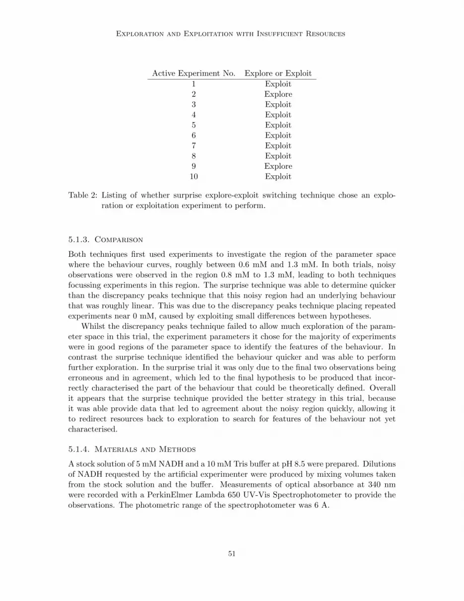
Table 2: Listing of whether surprise explore-exploit switching technique chose an explo-ration or exploitation experiment to perform.

5.1.3. Comparison

Both techniques first used experiments to investigate the region of the parameter spacewhere the behaviour curves, roughly between 0.6 mM and 1.3 mM. In both trials, noisyobservations were observed in the region 0.8 mM to 1.3 mM, leading to both techniquesfocussing experiments in this region. The surprise technique was able to determine quickerthan the discrepancy peaks technique that this noisy region had an underlying behaviourthat was roughly linear. This was due to the discrepancy peaks technique placing repeatedexperiments near 0 mM, caused by exploiting small differences between hypotheses.

Whilst the discrepancy peaks technique failed to allow much exploration of the param-eter space in this trial, the experiment parameters it chose for the majority of experimentswere in good regions of the parameter space to identify the features of the behaviour. Incontrast the surprise technique identified the behaviour quicker and was able to performfurther exploration. In the surprise trial it was only due to the final two observations beingerroneous and in agreement, which led to the final hypothesis to be produced that incor-rectly characterised the part of the behaviour that could be theoretically defined. Overallit appears that the surprise technique provided the better strategy in this trial, becauseit was able provide data that led to agreement about the noisy region quickly, allowing itto redirect resources back to exploration to search for features of the behaviour not yetcharacterised.

5.1.4. Materials and Methods

A stock solution of 5 mM NADH and a 10 mM Tris buffer at pH 8.5 were prepared. Dilutionsof NADH requested by the artificial experimenter were produced by mixing volumes takenfrom the stock solution and the buffer. Measurements of optical absorbance at 340 nmwere recorded with a PerkinElmer Lambda 650 UV-Vis Spectrophotometer to provide theobservations. The photometric range of the spectrophotometer was 6 A.

51


6. Evaluation in 2-dimensional Parameter Space

We now evaluate the experiment selection techniques within a 2-dimensional parameterspace. In each case the multiple hypotheses based hypothesis manager was used, combinedwith either the random, discrepancy peaks or surprise based technique for experiment se-lection. The protocol for the hypothesis manager remained the same as the 1-dimensionalversion, except that for performance 40 new hypotheses were created in each iteration(down from 200 in the 1-dimensional version), with the best 100 hypotheses kept into thenext round of experimentation (where the top 20% of the hypotheses were kept on eachiteration in the 1-dimensional version). Hypotheses were represented using a thin platespline (Wahba, 1990):

h = minn∑i,j

(y − f(x1, x2))2

+ λ

∫ ∞−∞

∫ ∞−∞

(f ′′(x1, x1)

2 + 2f ′′(x1, x2)2 + f ′′(x2, x2)

2)dx1dx2 (13)

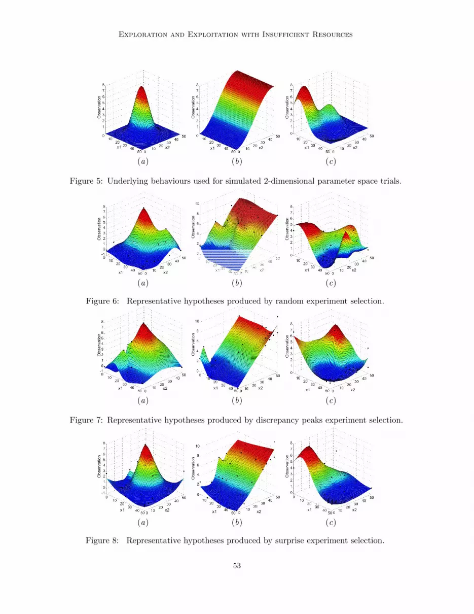
with a choice of smoothing parameters (λ ∈ {0.1, 0.2, 0.3, 0.4, 0.5}). All independent pa-rameters were coded between 0 and 1, from behaviours with uncoded x1 and x2 parametersboth ranging between 0 and 50. The underlying behaviours used are presented in Fig. 5,where (a) provides a single feature, (b) a behaviour where only the x2 factor provides arole in determining the response, and (c) a behaviour with two peaks and a trough. Ineach case the behaviours were between 0 and 8 on the dependent variable, so that the noiseparameters ε and φ could remain the same for both the 1 and 2-dimensional evaluations.

The three experiment selection strategies were tested over 100 trials per behaviour. Ineach behaviour, 5 initial experiments were performed, which were equally spaced around theparameter space ([0,0], [1,0], [0,1], [1,1] and [0.5,0.5] in coded values). After the exploratoryexperiments, a further 25 actively chosen experiments were performed per trial, where3 of the experiments produced erroneous observations. Gaussian noise was added to allobservations with ε = N(0, 0.52), whilst the noise applied to erroneous observations wasφ = N(3, 1). The techniques were again evaluated by comparing the mean over 100 trialsof the error between the most confident hypothesis and the true underlying behaviour.

6.1. Results

In the 2-dimensional problem, the results show there is less difference between the surpriseand random experiment selection techniques than in the 1-dimensional case, whilst the dis-crepancy peaks technique again generally performs the worst, as shown in Fig. 9. However,overall it appears that the surprise technique is still a more robust technique than the othersconsidered, with the technique providing significant improvements over a random strategyin two of the three underlying behaviours. In Fig. 6, 7 and 8, a comparison of most confi-dent hypotheses for each technique and behaviour after 25 active experiments are shown.In each case the error between the hypothesis shown and the true underlying behaviour isrepresentative of the mean error given in Fig. 9.

For the single feature behaviour, A, the random technique outperforms the surprisetechnique between the 7th and 23rd active experiments, as shown in Fig. 9(a). During

52


(a) (b) (c)

Figure 5: Underlying behaviours used for simulated 2-dimensional parameter space trials.

(a) (b) (c)

Figure 6: Representative hypotheses produced by random experiment selection.

(a) (b) (c)

Figure 7: Representative hypotheses produced by discrepancy peaks experiment selection.

(a) (b) (c)

Figure 8: Representative hypotheses produced by surprise experiment selection.

53


0

2

4

6

8

10

12

14

0 5 10 15 20 25

E


Surprise

Random

Peaks

(a)

0

0.2

0.4

0.6

0.8

1

1.2

1.4

1.6

0 5 10 15 20 25

E


(b)

0

0.5

1

1.5

2

2.5

3

0 5 10 15 20 25

E


(c)

Figure 9: Mean error from 100 trials over number of active experiments performed, for thethree behaviours and three experiment selection techniques being evaluated inthe 2-dimensional parameter space evaluation. The error over time is shown forthe active experiments that occur after the 5 initial experiments. In (a) the resultfor the behaviour shown in Fig. 5(a) is shown, (b) corresponds to Fig. 5(b) and(c) corresponds to Fig. 5(c).

these experiments, the surprise technique spends more time investigating smaller differ-ences between the hypotheses, causing a greater amount of exploitation early on than isperhaps necessary. Whilst the random technique is able to explore the parameter spacemore early on, allowing it to form a better general understanding of the behaviour quickerthan the surprise technique. However, the random technique can perform poorly if it sam-ples a region of the parameter space only once and obtains an erroneous observation, whichcan cause it to include an additional feature in the prediction that is not present in theunderlying behaviour, as shown in Fig. 6(a). The discrepancy peaks technique performspoorly throughout, by over exploiting the information obtained rather than exploring. Thiscauses discrepancy peaks technique to continually investigate small differences between thehypotheses, caused by the Gaussian noise applied to each observation.

For the single factor behaviour, B, the initial 5 data points, if error free, are capable ofproviding all of the techniques with data suitable for producing a good representation of thebehaviour. Therefore this behaviour tests the ability of the experiment selection techniquesto deal with erroneous observations in a 2-dimensional parameter space. The random tech-nique fails to improve the performance of the most confident hypothesis throughout the25 actively chosen experiments. In part this is caused by the technique not investigating

54


erroneous observations, so any improvements to understanding the behaviour are lost by er-roneous observations that misguide hypothesis formation. The surprise technique performswell early on, as it is able to investigate erroneous observations. However the mean errorincreases again between 7 and 15 experiments because the technique over investigates someobservations, causing the hypotheses to overfit some of the noise. The discrepancy peakstechnique also suffers the problem of over sampling a region, causing lots of hypotheses withdifferences of opinion in a small area, which leads to hypotheses overfitting in those areasthe ε noise applied to the observations. However, over time the discrepancy peaks techniquelowers the error to slightly below the surprise error in the latter stages of experimentation.By 25 experiments the performance of the surprise and discrepancy peaks techniques arenearly equal.

For the behaviour with multiple features, C, the resources available were too few to get agood representation of the behaviour. The surprise and random techniques reduce the errorat a similar rate for the first 18 active experiments. However after 18 active experimentsthe error for the random technique levels out, whilst it continues to reduce for the surprisetechnique. In the random technique the experiments are spread out across the parameterspace, allowing for the different features to be identified quickly, albeit at a low resolution.However, as the experiments are not directed, increasing the understanding of any partic-ular behaviour is by chance and potentially erroneous observations are ignored. These twofactors prevent the error from reducing further later on in experimentation. The surprisetechnique through performing exploitation experiments, performs more experiments nearthe features it discovers, causing better representations of the behaviour to be formed. Ad-ditionally, the technique is able to investigate and identify erroneous observations, whilstalso performing experiments to further search the parameter space. The discrepancy peakstechnique performs worse than the other two techniques, because it over exploits and be-comes focussed in particular regions of the parameter space where the first unexpectedbehaviours were obtained. Unlike the other two behaviours where all techniques provideda somewhat representative prediction of the underlying behaviour, the surprise based tech-nique is the only technique to provide a good representation of underlying behaviour C,shown in Fig. 5(c), 6(c), 7(c) and 8(c).

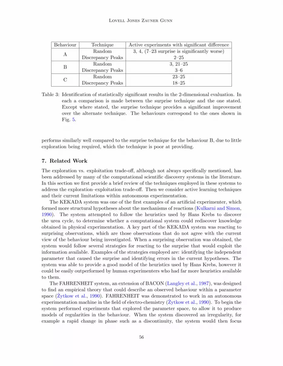
Like the 1-dimensional case, the results for the 2-dimensional parameter space have beenanalysed using a two-tailed t-test with α = 0.05 to determine if the results are significantat the 95% confidence interval, shown in Table 3. The surprise technique provided sig-nificant improvements over a random selection strategy for behaviours B and C, althoughonly in the latter stages of experimentation. These improvements are in part due to thesurprise technique being able to better identify erroneous observations than the randomtechnique. Additionally the surprise technique is able to investigate the new features itdiscovers further, which allows it to provide a better representation of the more complexbehaviour C. The random strategy performs significantly better than the surprise techniquefor the majority of the experimentation performed using behaviour A. This is due to therandom technique being able to explore the parameter space more, where the surprise tech-nique spends some additional time investigating small differences between the hypothesesthat only provide small benefits for developing a representation of the behaviour. Thediscrepancy peaks technique performs significantly worse than the surprise technique forbehaviours A and C by the end of the experimentation performed. However, the technique

55


Behaviour Technique Active experiments with significant difference

ARandom 3, 4, (7–23 surprise is significantly worse)

Discrepancy Peaks 2–25

BRandom 3, 21–25


CRandom 23–25


Table 3: Identification of statistically significant results in the 2-dimensional evaluation. Ineach a comparison is made between the surprise technique and the one stated.Except where stated, the surprise technique provides a significant improvementover the alternate technique. The behaviours correspond to the ones shown inFig. 5.

performs similarly well compared to the surprise technique for the behaviour B, due to littleexploration being required, which the technique is poor at providing.

7. Related Work

The exploration vs. exploitation trade-off, although not always specifically mentioned, hasbeen addressed by many of the computational scientific discovery systems in the literature.In this section we first provide a brief review of the techniques employed in these systems toaddress the exploration–exploitation trade-off. Then we consider active learning techniquesand their current limitations within autonomous experimentation.

The KEKADA system was one of the first examples of an artificial experimenter, whichformed more structural hypotheses about the mechanisms of reactions (Kulkarni and Simon,1990). The system attempted to follow the heuristics used by Hans Krebs to discoverthe urea cycle, to determine whether a computational system could rediscover knowledgeobtained in physical experimentation. A key part of the KEKADA system was reacting tosurprising observations, which are those observations that do not agree with the currentview of the behaviour being investigated. When a surprising observation was obtained, thesystem would follow several strategies for reacting to the surprise that would exploit theinformation available. Examples of the strategies employed are: identifying the independentparameter that caused the surprise and identifying errors in the current hypotheses. Thesystem was able to provide a good model of the heuristics used by Hans Krebs, however itcould be easily outperformed by human experimenters who had far more heuristics availableto them.

The FAHRENHEIT system, an extension of BACON (Langley et al., 1987), was designedto find an empirical theory that could describe an observed behaviour within a parameterspace (Zytkow et al., 1990). FAHRENHEIT was demonstrated to work in an autonomousexperimentation machine in the field of electro-chemistry (Zytkow et al., 1990). To begin thesystem performed experiments that explored the parameter space, to allow it to producemodels of regularities in the behaviour. When the system discovered an irregularity, forexample a rapid change in phase such as a discontinuity, the system would then focus

56


experiments on investigating the extent of the irregularity, producing separate models forthe regions of regularity adjacent to the irregularity. However this system would require alarge number of experiments to be performed to provide the data required.

A system developed to automate a chemistry workstation, employed a grid search withdecreasing grid size as part of its strategy to manage the exploration–exploitation trade-off (Dixon et al., 2002). The goal of the system was to discover the parameters that producedthe highest yield within the experiment parameter space. Initially experiments were placedspread out across the parameter space to provide exploration by a grid with large gridsquares. The size of the grid squares decreased over subsequent experiments, to provide amore detailed analysis of the behaviour. Additionally a simplex based experiment selectiontechnique was employed in later stages of experimentation, where experiments would focustowards areas of the parameter space where previously high yields were obtained (Du andLindsey, 2002). Like many evolutionary algorithms, the technique had the potential forbecoming stuck within a local maxima.

Scouting was an evolutionary algorithm that evolved parameters based on an adap-tive measure of surprise, which was able to manage the trade-off between exploration andexploitation (Pfaffmann and Zauner, 2001). Like KEKADA, surprising observations werethose that differed from the hypothesis under consideration. When no observations weresurprising, experiments would be placed randomly within the parameter space. When asurprising observation was obtained, the evolutionary algorithm would then place experi-ments near the surprising observation. Importantly, as more experiments were placed nearthe initially surprising observation, so the model would better represent the behaviour andthe observation would become less surprising. This adaptivity of surprise, meant that oncesufficient information had been obtained to investigate why the observation was surprising,the algorithm would again place experiments in other areas of the parameter space, au-tomatically addressing the exploration-exploitation trade-off. The scouting approach wasdemonstrated within an autonomous experimentation machine to characterise enzymaticresponse behaviours (Matsumaru et al., 2002). A problem with this technique was that ifan observation was erroneous, then it could remain surprising as subsequent observationswould not agree with it, meaning that the system could remain performing exploitationexperiments in that region.

The robot scientist (King et al., 2004) does not algorithmically consider the trade-offbetween exploration and exploitation. Instead the system is provided with a large body ofinformation within a relatively small domain, which is then used to formulate hypothesesthat can be tested to determine their validity. Essentially the initial information providedby the user is the only exploration that occurs. The active learning technique the systemuses to select experiments to examine the hypotheses is purely exploitative, by choosingexperiments that will reduce the likely cost to determine the most representative hypothesis.

Another technique that investigates automatically characterising enzymatic responsecharacterisation, performs a largely exploration focussed experiment selection (Bonowskiet al., 2010). Initially the technique is explorative through placing experiments using aspace fitting algorithm to ensure a good distribution of experiments across the experimentparameter space. Later experiments combine exploitation and exploration through placingexperiments where the uncertainty in the hypothesis is greatest, but also explorative throughrequiring experiments to fulfil a minimum distance requirement between experiments in

57


the parameter space. The minimum distance required decreases over time, to allow finerexamination of the parameter space. However the technique does not consider erroneousobservations.

7.1. Active Learning

Active learning seeks to address the same issues as those in autonomous experimentation.That is to minimise the number of labels to obtain, or experiments to perform, whilst max-imising the information obtained. In comparison to present autonomous experimentationtechniques, active learning is more theoretically grounded and mathematically sound thanthe often ad-hoc techniques found in autonomous experimentation. However at presentthe theoretical assumptions made in active learning mean the problems addressed are notalways representative of physical experimentation, which limits their potential applications.In particular the assumption that experiments occur without noise, is an assumption thatis made too frequently (Cohn et al., 1994; Freund et al., 1997), or that a hypothesis isalready in consideration that provides a suitable representation of the behaviour being in-vestigated (MacKay, 1992; Settles, 2009).

The work by MacKay (1992) places experiments where the predicted information gain ishighest, either in a single hypothesis or to discriminate between multiple models. In order todo this, the assumption is made that at any particular point in the experimentation, a modelexists that is representative of the underlying behaviour being investigated. This makesexperiment selection purely exploitation based and is honing in on the most appropriatemodel or hypothesis. In physical experimentation this will often not be the case. Whilst themethod for discriminating between hypotheses proposed by MacKay is useful in autonomousexperimentation, and is similar to the discrepancy function we use in Eqn. 3, the techniqueas a whole cannot be used as is within physical experimentation, due to the assumptionabout a complete model space.

Query-by-committee provides a way of managing the uncertainty in predictions throughallowing an ensemble of hypotheses to be considered in parallel, similar to how the multiplehypotheses are used within the approach considered here (Seung et al., 1992). The tech-nique takes an ensemble of hypotheses and performs experiments in the locations wherethere is the maximal disagreement between hypotheses. The disagreement is consideredmaximal where there are equal votes for the two options within a binary classification prob-lem. However the query-by-committee is stated to have limitations that restrict the use ofthe algorithm within practical applications, with the primary limitation being the assump-tion that experiments are noise free (Freund et al., 1997). The idea of considering multiplehypotheses is important in managing the uncertainty presented within autonomous exper-imentation problems, therefore query-by-committee is a highly appropriate technique toapply within such active learning tasks. Although alterations are required to the techniquein terms of hypothesis management and discrepancy calculation, like those presented here,before this technique can be more widely used within autonomous experimentation.

Active learning has considered the possibility of erroneous observations, described inthe literature as noisy oracles (Settles, 2009). However research into this particular area iscurrently extremely limited and do not address the issue found in experimentation whereerroneous observations occur sporadically, with no particular distribution or consistency.

58


8. Conclusion

In physical experimentation, the costs per experiment prevent large numbers of observationsfrom being obtained. With the validity of observations not guaranteed, experiments must beperformed that test the validity of the hypotheses produced and also search the parameterspace under investigation for features of the behaviour not yet discovered. This trade-offbetween feature discovery and hypothesis evaluation is an exploration–exploitation trade-off,where differences between competing hypotheses is used in the exploitation. The resourcesavailable prevent a large number of repeated experiments in an area to get a highly accurateprediction. Likewise the resources limit the exploration that can be performed to find allthe different features of the behaviour. Techniques are therefore required that will search forfeatures of the behaviour under investigation, whilst ensuring a reasonable level of confidencethat the hypothesised feature observed is genuine.

To manage this trade-off we consider a technique that is similar to how successful hu-man experimenters address the problem in physical experimentation, by using the surpriseof the last observation obtained to determine whether the next experiment will explore orexploit. A Bayesian formulation of surprise has been used, where an exploration experimentis performed when the last experiment was not surprising and an exploitation experimentis performed when the last experiment was surprising. This use of surprise ensures thatexperiments are performed to evaluate hypotheses when an observation is discovered thatthe hypotheses did not expect, to determine why the hypotheses did not expect that obser-vation, either due to the observation being erroneous or the hypotheses inaccurate. Whilstwhen observations are obtained that are similar to the predictions of the most confidenthypotheses under consideration, then exploration is performed to look for features of thebehaviour not yet captured by the hypotheses.

Expanding to higher dimensions, the surprise technique was in some cases able to pro-vide a significant improvement over the alternate techniques considered. However the degreeof benefit was less than in the 1-dimensional case. A limitation of the surprise technique inthe higher dimension problems, was that it performs little exploration early on. As the thinplate splines tended to overfit observation noise more than the smoothing splines did with1-dimensional data, there was greater discrepancy between the hypotheses, which causedthe surprise technique to exploit more often, especially in early experiments where most ob-servations would be surprising to the hypotheses. This led to some of the early experimentsbeing focussed within a particular area. However, unlike the discrepancy peaks techniquethat could also focus the placement of experiments within a small area, the surprise tech-nique adapted over time and explored the parameter space, leading to it providing moreaccurate hypotheses than the other techniques later on in experimentation. The surprisetechnique could benefit from additional initial exploration, however care would have to betaken to ensure that this exploration does not bias particular regions of the parameter space.

Acknowledgments

The reported work was supported in part by a Microsoft Research Faculty Fellowship toKPZ. This work was supported in part by the IST Programme of the European Community,under the PASCAL2 Network of Excellence, IST-2007-216886. This publication only reflectsthe authors’ views.

59


References

P. Auer. Using confidence bounds for exploitation-exploration trade-offs. Journal of Ma-chine Learning Research, 3:397–422, 2002.

F. Bonowski, A. Kitanovic, P. Ruoff, J. Holzwarth, I. Kitanovic, V. N. Bui, E. Lederer,and S. Wolfl. Computer controlled automated assay for comprehensive studies of enzymekinetic parameters. PLos ONE, 5(5):1–10, 2010.

T. C. Chamberlin. The method of multiple working hypotheses. Science (old series), 15:92–96, 1890. Reprinted in: Science, v. 148, p. 754–759, May 1965.

D. Cohn, L. Atlas, and R. Ladner. Improving generalization with active learning. MachineLearning, 15:201–221, 1994.

J. M. Dixon, H. Du, D. G. Cork, and J. S. Lindsey. An experimental planner for performingsuccessive focused grid searches with an automated chemistry workstation. Chemometricsand Intelligent Laboratory Systems, 62:115–128, 2002.

H. Du and J. S. Lindsey. An approach for parallel and adaptive screening of discretecompounds followed by reaction optimization using an automated chemistry workstation.Chemometrics and Intelligent Laboratory Systems, 62:159–170, 2002.

Y. Freund, H. S. Seung, E. Shamir, and N. Tishby. Selective sampling using the query bycommittee algorithm. Machine Learning, 28:133–168, 1997.

L. Itti and P. Baldi. Bayesian surprise attracts human attention. Vision Research, 49:1295–1306, 2009.

R. D. King, K. E. Whelan, F. M. Jones, P. G. K. Reiser, C. H. Bryant, S. H. Muggleton,Douglas B. Kell, and Stephen G. Oliver. Functional genomic hypothesis generation andexperimentation by a robot scientist. Nature, 427:247–252, 2004.

D. Kulkarni and H. A. Simon. Experimentation in machine discovery. In J. Shrager andP. Langley, editors, Computational Models of Scientific Discovery and Theory Formation,pages 255–273. Morgan Kaufmann Publishers, San Mateo, CA, 1990.

P. Langley, H. A. Simon, G. L. Bradshaw, and J. M. Zytkow. Scientific Discovery: compu-tational explorations of the creative processes. MIT Press, 1987.

C. J. Lovell, G. Jones, S. R. Gunn, and K.-P. Zauner. An artificial experimenter for enzy-matic response characterisation. In 13th International Conference on Discovery Science,pages 42–56, Canberra, Australia, 2010.

C. J. Lovell, G. Jones, S. R. Gunn, and K.-P. Zauner. Autonomous experimentation:Active learning for enzyme response characterisation. JMLR: Workshop and ConferenceProceedings, 16:141–154, 2011.

D. J. C. MacKay. Information–based objective functions for active data selection. NeuralComputation, 4:589–603, 1992.

60


N. Matsumaru, S. Colombano, and K.-P. Zauner. Scouting enzyme behavior. In D. B.Fogel, M. A. El-Sharkawi, X. Yao, G. Greenwood, H. Iba, P. Marrow, and M. Shackleton,editors, 2002 World Congress on Computational Intelligence, May 12-17, pages CEC19–24, Honolulu, Hawaii, 2002. IEEE, Piscataway, NJ.

D. L. Nelson and M. M. Cox. Lehninger Principles of Biochemistry. W. H. Freeman andCompany, New York, USA, 5th edition, 2008.

J. O. Pfaffmann and K.-P. Zauner. Scouting context-sensitive components. InD. Keymeulen, A. Stoica, J. Lohn, and R. S. Zebulum, editors, The Third NASA/DoDWorkshop on Evolvable Hardware—EH-2001, pages 14–20, Long Beach, July 2001. IEEEComputer Society, Los Alamitos.

B. Settles. Active learning literature survey. Technical report, University of Wisconsin-Madison, 2009.

H. S. Seung, M. Opper, and H. Sompolinsky. Query by committee. In Proceedings of theACM Workshop on Computational Learning Theory, pages 287–294, 1992.

G. Wahba. Spline Models for Observational Data, volume 59 of CBMS-NSF Regional Con-ference series in applied mathematics. Society for Industrial and Applied Mathematics,Philadelphia, PA, 1990.

J. M. Zytkow, J. Zhu, and A. Hussam. Automated discovery in a chemistry laboratory.In Proceedings of the 8th National Conference on Artificial Intelligence, pages 889–894,Boston, MA, 1990. AAAI Press / MIT Press.

61

exploration and exploitation with insufficient resources

Documents