International Journal of Solids and Structures 40 (2003) 4281–4297

www.elsevier.com/locate/ijsolstr

Contrasting probabilistic and anti-optimization approachesin an applied mechanics problem

I. Elishakoff a, M. Zingales b,*

a Department of Mechanical Engineering, Florida Atlantic University, 777 Glades Road, Boca Raton, FL 33431-0991, USAb Department of Structural and Geotechnical Engineering, Ingegneria Strutturale e Geotecnica, Universit�aa di Palermo,

Viale delle Scienze, I-90128 Palermo, Italy

Received 26 March 2003; received in revised form 26 March 2003

Abstract

Probabilistic and non-probabilistic, anti-optimization analyses of uncertainty are contrasted in this study. Specifi-

cally, the comparison of these two competing approaches is conducted for an uniform column, with initial geometric

imperfection, subjected to an impact axial load. The reliability of the column is derived for the cases when the initial

imperfections posses either (a) uniform probability density, (b) truncated exponential density or (c) generic truncated

probability density. The problem is also analyzed in the context of an interval analysis. It is shown that in, the most

important near-unity reliability range these two approaches tend to each other. Since the interval analysis constitutes a

much simpler procedure than the probabilistic approach, it is argued that the former is advantageous over the latter in

some circumstances.

� 2003 Elsevier Science Ltd. All rights reserved.

Keywords: Probabilistic; Reliability

1. Introduction

According to Einstein, ‘‘so far as the laws of mathematics refer to reality they are not certain. And so far

as they are certain they does not refer to reality’’. How much more this statement appears to apply to

engineering, where numerous uncertain factors are encountered, almost in every problem. The pertinent

question arises on how to model this uncertainty. It is nowadays widely accepted that there are three

competing methods of describing uncertainty, namely, probabilistic method, fuzzy sets based approach,

and the method which is referred to as anti-optimization (Elishakoff and Ben-Haim, 1990) or as guaranteed

approach by Kurzhanski (1977) and by Chernousko (1994). Each of these approaches has generatednumerous research papers and monographs. Yet the systematic comparisons between these three approaches

are still missing. Naturally, there may be a strong argument put forward against such a comparison, in the

* Corresponding author. Tel.: +39-0916568458; fax: +39-0916568407.

E-mail address: zingales@diseg.unipa.it (M. Zingales).

0020-7683/03/$ - see front matter � 2003 Elsevier Science Ltd. All rights reserved.

doi:10.1016/S0020-7683(03)00196-3

4282 I. Elishakoff, M. Zingales / International Journal of Solids and Structures 40 (2003) 4281–4297

first place. Indeed, these three approaches provide judgements of different kind: probabilistic approach

furnishes the reliability of the structure, namely the probability that the structure�s stress, strains or dis-

placements will not take values over some safe threshold. Fuzzy-sets-based approach yields via the concept

of a membership function, the safety margin. Anti-optimization (or guaranteed approach) provides withleast favorable, maximum displacements which can be contrasted with the threshold values. If the maxi-

mum response does not cross the threshold, we can guarantee that the failure will not occur. This corres-

ponds to the statement that if the least favorable, or an anti-optimized, response will be below the failure

boundary, the successful performance will be secured.

This particular thought, namely that three approaches provide with different types of answers, precluded

the very attempt to compare them for a long time. First numerical comparison have been performed in-

dependently by Elishakoff et al. (1994) and Kim et al. (1993) in different but complementary contexts: the

former study dealt with non-linear static buckling, whereas the latter investigation dealt with linear dynamicresponse. In the paper by Elishakoff et al. (1994) for certain regions of variations of the parameters, the

design values of the buckling loads, obtained via applications of two alternative approaches were found to be

extremely close to each other. In the paper by Kim et al. (1993) the design value corresponding to the mean

plus three times standard deviation, was adopted. Recently, Elishakoff and Li (1999) studied a benchmark

static problem, leading to direct contrast of the probabilistic and non-probabilistic analyses of the uncer-

tainty. This study is devoted to systematic comparison of these two approaches in the dynamic environment.

We will consider impact buckling of uniform columns possessing uncertain initial imperfections.

2. Problem formulation

The differential equation for the uniform column (Fig. 1) under axial impact load

P ðtÞ ¼ P hti0 ð1Þ

reads

EIo4wox4

þ P ðtÞ o2wox2

þ mAo2wot2

¼ �P ðtÞ o2w0

ox2ð2Þ

with E ¼ modulus of elasticity, I ¼ moment of inertia, m ¼ mass density, A ¼ cross-sectional area,

P ðtÞ ¼ axial load, w0ðxÞ ¼ initial imperfection, constituting a small deviation of the initial shape of the

unstressed column, wðxÞ ¼ additional transverse deflection of the column�s axis, so that

wTðx; tÞ ¼ w0ðxÞ þ wðx; tÞ; ð3Þ

represents a total displacement. In Eq. (1) hti0 is a singularity function, namely, a unit step function

hti0 ¼ 0; t < 0;1; tP 0:

�ð4Þ

Fig. 1. Description of the structural model.

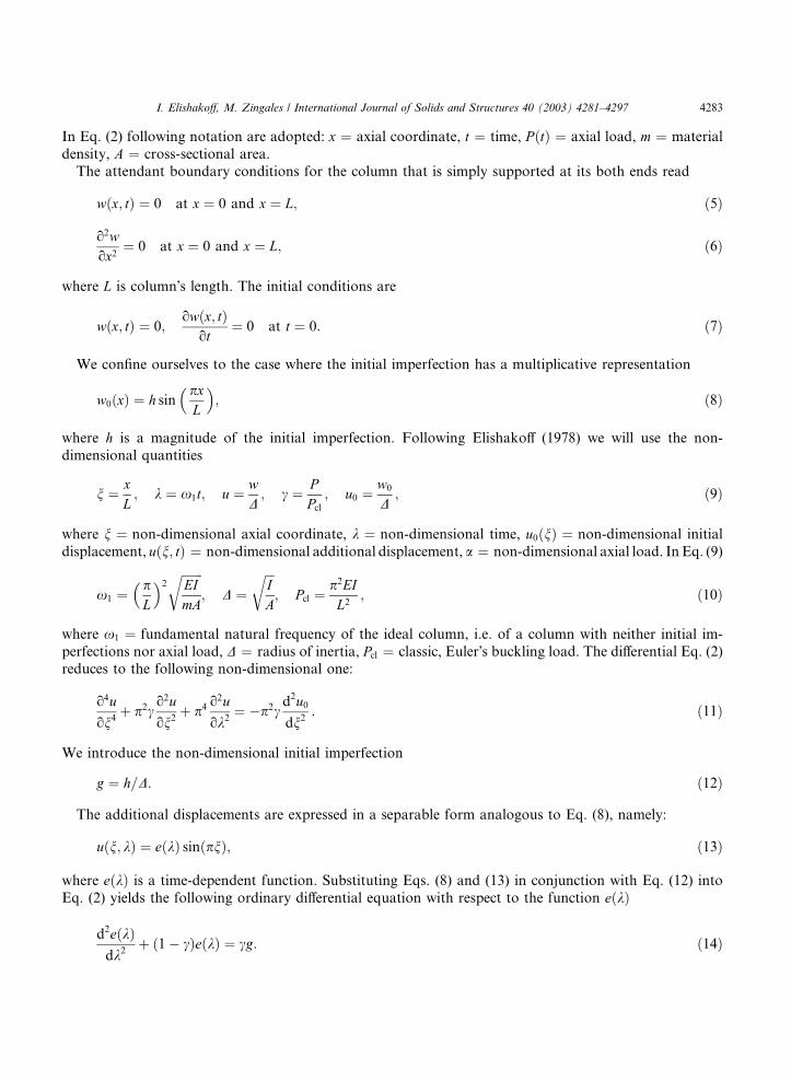
I. Elishakoff, M. Zingales / International Journal of Solids and Structures 40 (2003) 4281–4297 4283

In Eq. (2) following notation are adopted: x ¼ axial coordinate, t ¼ time, P ðtÞ ¼ axial load, m ¼ material

density, A ¼ cross-sectional area.

The attendant boundary conditions for the column that is simply supported at its both ends read

wðx; tÞ ¼ 0 at x ¼ 0 and x ¼ L; ð5Þ

o2wox2

¼ 0 at x ¼ 0 and x ¼ L; ð6Þ

where L is column�s length. The initial conditions are

wðx; tÞ ¼ 0;owðx; tÞ

ot¼ 0 at t ¼ 0: ð7Þ

We confine ourselves to the case where the initial imperfection has a multiplicative representation

w0ðxÞ ¼ h sinpxL

� �; ð8Þ

where h is a magnitude of the initial imperfection. Following Elishakoff (1978) we will use the non-

dimensional quantities

n ¼ xL; k ¼ x1t; u ¼ w

D; c ¼ P

Pcl; u0 ¼

w0

D; ð9Þ

where n ¼ non-dimensional axial coordinate, k ¼ non-dimensional time, u0ðnÞ ¼ non-dimensional initial

displacement, uðn; tÞ ¼ non-dimensional additional displacement, a ¼ non-dimensional axial load. In Eq. (9)

x1 ¼pL

� �2 ffiffiffiffiffiffiffiEImA

r; D ¼

ffiffiffiIA

r; Pcl ¼

p2EIL2

; ð10Þ

where x1 ¼ fundamental natural frequency of the ideal column, i.e. of a column with neither initial im-

perfections nor axial load, D ¼ radius of inertia, Pcl ¼ classic, Euler�s buckling load. The differential Eq. (2)reduces to the following non-dimensional one:

o4u

on4þ p2c

o2u

on2þ p4 o

2u

ok2¼ �p2c

d2u0dn2

: ð11Þ

We introduce the non-dimensional initial imperfection

g ¼ h=D: ð12Þ

The additional displacements are expressed in a separable form analogous to Eq. (8), namely:

uðn; kÞ ¼ eðkÞ sinðpnÞ; ð13Þ

where eðkÞ is a time-dependent function. Substituting Eqs. (8) and (13) in conjunction with Eq. (12) into

Eq. (2) yields the following ordinary differential equation with respect to the function eðkÞ

d2eðkÞdk2

þ ð1� cÞeðkÞ ¼ cg: ð14Þ

4284 I. Elishakoff, M. Zingales / International Journal of Solids and Structures 40 (2003) 4281–4297

The solution, satisfying the initial conditions (Eq. (7)), is

eðkÞ ¼

cg1� c

ðcoshðrkÞ � 1Þ; c > 1;

1

2gk2; c ¼ 1;

cg1� c

ð1� cosðrkÞÞ; c < 1:

8>>>>><>>>>>:ð15Þ

The non-dimensional total displacement zðn; kÞ equals

zðn; kÞ ¼ wTðx; tÞ=D ¼ vðkÞ sinðpnÞ ð16Þ

with vðkÞ being a function of a non-dimensional time k alone

vðkÞ ¼ cg1� c

coshðrkÞ

� 1

c

�; c > 1; ð17aÞ

vðkÞ ¼ gðk2 þ 2Þ=2; c ¼ 1; ð17bÞ

vðkÞ ¼ cg1� c

1

c

� cosðrkÞ

�; c < 1: ð17cÞ

Next sections will deal with various uncertainty analyses.

3. Probabilistic analysis

We treat the uncertain initial imperfection magnitude as a random variable with specified probability

distribution function:

FGðgÞ ¼ ProbðG6 gÞ: ð18Þ

We are interested in finding the survival reliability of the structure, which is defined in general form as the

probability that the structure will perform its specified mission. Herewith we adopt Hoff�s (1965) criterion:

‘‘A structure is in a stable state if admissible finite disturbances of initial state of static or dynamic equi-

librium are followed by displacements whose magnitude remains within allowable bounds during the

required lifetime of the structure.’’

Within this definition, we introduce the admissible state as follows:

�d 6 zðn; kÞ6 c; ð19Þ

where c is the non-dimensional upper bound, and d is the non-dimensional lower bound of the safety

region. On the other hand, the inequalities

maxn

zðn; kÞ > c or maxn

zðn; kÞ < �d; ð20Þ

mean unsafe regions, or, as defined by Hoff, as regions of impact buckling. Hereinafter we denote random

variables with capital letters, whereas the possible values they take on are designated with lower case

notation. Reliability is defined as a probability that the event described in Eq. (19) takes place

RðkÞ ¼ Prob

� d 6max

nZðn; kÞ6 c

�: ð21Þ

I. Elishakoff, M. Zingales / International Journal of Solids and Structures 40 (2003) 4281–4297 4285

k being a pre-chosen non-dimensional time. Since

maxn

Zðn; kÞ ¼ Zð1=2; kÞ ¼ V ðkÞ; ð22Þ

the reliability becomes

RðkÞ ¼ Prob�� d 6 V ðkÞ6 c

: ð23Þ

Note that V ðkÞ is a random function of k, and is represented as a product:

V ðkÞ ¼ GaðkÞ; ð24Þ

where G is a random variable and aðkÞ is a deterministic function,

aðkÞ ¼ c1� c

cosðrkÞ

� 1

c

�; c < 1; ð25aÞ

aðkÞ ¼ 1

2ðk2 þ 2Þ; c ¼ 1; ð25bÞ

aðkÞ ¼ c1� c

coshðrkÞ

� 1

c

�; c > 1: ð25cÞ

Reliability, as per in Eq. (23), becomes:

RðkÞ ¼ Prob V ðkÞ�

6 c � Prob V ðkÞ

�6 � d

¼ Prob G

6

c

aðkÞ

!� Prob G

6 � d

aðkÞ

!; ð26Þ

since aðkÞ is a positive-valued function. In terms of probability distribution function FGðgÞ, Eq. (26) is

rewritten as:

RðkÞ ¼ FGc

aðkÞ

!� FG

� d

aðkÞ

!: ð27Þ

Eq. (27) depends, in general, of the specific form of the probability distribution function FGðgÞ. The

influences of the specified probability distribution function over the design of the geometric characteristic

of the column will be the objective of the next sections.

4. Uniformly distributed random initial imperfections

Let us first consider the case when the initial imperfection amplitude G (Fig. 1) possesses an uniformprobability density function over the interval ½a1; a2 and vanishes elsewhere. The probability distribution

function FGðgÞ reads

FGðgÞ ¼1

a2 � a1

hg�

� a1i1 � hg � a2i1�; ð28Þ

where hg � ai1 is a singularity function

hg � ai1 ¼ 0; g < a;g � a; gP a:

�ð29Þ

4286 I. Elishakoff, M. Zingales / International Journal of Solids and Structures 40 (2003) 4281–4297

The reliability of the column becomes

RðkÞ ¼ 1

a2 � a1

c

aðkÞ

*0@ � a1

+1

� c

aðkÞ

*� a2

+11A� 1

a2 � a1

*0@ � d

aðkÞ� a1

+1

�*

� d

aðkÞ� a2

+11A:

ð30Þ

Hereinafter, for the sake of simplicity we take a1 P 0; a2 P 0. Since the arguments in third and fourth termsin Eq. (30) are negative, they vanish. We are left with the following expression

RðkÞ ¼ 1

a2 � a1

c

aðkÞ

*0@ � a1

+1

� c

aðkÞ

*� a2

+11A: ð31Þ

We are interested in designing the system, namely, choosing the radius q of a circular cross-section suchthat the reliability RðkÞ will be no less than some codified reliability rc:

RðkÞP rc: ð32Þ

Consider first a sub-case when the applied axial load exceeds the classical buckling load, so that

a ¼ PPcl

¼ PL2

p2EI¼ M

q4> 1; M ¼ 4PL2

p3E; ð33Þ

where M is a load-dependent parameter. In virtue of Eq. (25), the reliability reads

RðkÞ ¼ 1

a2 � a1

cð1� q4=MÞcoshðrkÞ � q4=M

*0@ � a1

+11A� 1

a2 � a1

cð1� q4=MÞcoshðrkÞ � q4=M

*0@ � a2

+11A: ð34Þ

Let us closely investigate this expression: if for the pre-selected, non-dimensional time instant k, the ar-

gument of the singularity functions in Eq. (34) satisfies the inequality

cð1� q4=MÞcoshðrkÞ � q4=M

< a1; ð35Þ

then the reliability vanishes identically. On the other hand, if

cð1� q4=MÞcoshðrkÞ � q4=M

> a2; ð36Þ

then the reliability equals unity. In the intermediate range, i.e. for

a1 6cð1� q4=MÞ

coshðrkÞ � q4=M6 a2; ð37Þ

the reliability varies between zero to unity. Generally, in engineering practice, the codified reliability rc isnot taken to be unity. Rather, it is a pre-chosen quantity in an extremely close vicinity of unity. For rctending to unity from below, the inequality in Eq. (37) is valid. Hence the argument in the second term in

Eq. (34) is negative. Therefore, it vanishes, and we are left with:

RðkÞ ¼ 1

a2 � a1

cð1� q4=MÞcoshðrkÞ � q4=M

*� a1

+1

: ð38Þ

I. Elishakoff, M. Zingales / International Journal of Solids and Structures 40 (2003) 4281–4297 4287

In order the reliability to tend to unity from below, it is necessary and sufficient that:

limq!qd

cð1� q4=MÞcoshðrkÞ � q4=M

¼ a2; ð39Þ

where qd is the design value of the cross-section�s radius. For it we obtain the following equation:

cð1� q4d=MÞ

cosh kffiffiffiffiffiffiffiffiffiffiffiffiffiffiffiffiffiffiffiffiM=q4

d � 1p� �

� q4d=M

¼ a2: ð40Þ

It should be noted that the non-dimensional time parameter k is proportional to the radius, through

Eq. (10), expressed as

k ¼ 1

2

pL

� �2 ffiffiffiffiEm

r( )�ttqd: ð41Þ

Eq. (40) is a transcendental equation in terms of qd, once the time instant �tt at which reliability rc is desired,the failure boundary c, and other parameters are fixed. Design process requires to obtain the cross-sectional

radius qd as a function of these quantities qd ¼ qdð�tt; c;E;m; LÞ either analytically or numerically. It is

advantageous, however, to view Eq. (40) as a function of the failure boundary c as depending upon the

radius qd and the remaining parameters

cðqd;�tt;E;m; LÞ ¼a2 cosh k

ffiffiffiffiffiffiffiffiffiffiffiffiffiffiffiffiffiffiffiffiM=q4

d � 1p� �

� q4d=M

n o1� q4

d=M: ð42Þ

This relationship enables the design of the column graphically. One gets a curve c vs qd with otherparameters fixed. Once such curve is drawn, the determination of the required cross-sectional radius qd

becomes a straightforward task: one specifies the failure boundary c and reaches the correspondent radius

in the graph.

Two other sub-cases, associatedwith P ¼ Pcl or P > Pcl, respectively, are dealt with in a perfect analogy. ForP ¼ Pcl the design value of the cross-section�s radius is immediately expressed as the equation qd ¼

ffiffiffiffiffiM4

p. Then

cðqd;�tt;E;m; LÞ ¼a2

2

pL

� �4 Em�tt2

ffiffiffiffiffiM

p�þ 2

�; ð43Þ

whereas for P < Pcl this equation takes the following form:

cðqd;�tt;E;m; LÞ ¼a2 cos k

ffiffiffiffiffiffiffiffiffiffiffiffiffiffiffiffiffiffiffiffi1�M=q4

d

p� �� q4

d=Mn o

1� q4d=M

: ð44Þ

The results of sample calculations are presented in Figs. 2–4 portraying reliability RðkÞ vs non-dimen-

sional time k for P < Pcl, P ¼ Pcl, P > Pcl, respectively. In the following we will assume the following me-

chanical and geometrical parameters of the column L ¼ 10:0 m, E ¼ 2:1� 106 kg/cm2, m ¼ 2:1� 10�3/9.81

kg s2/cm4. The axial load P is set at P ¼ 3000 kg. As it is seen from Fig. 2, RðkÞ does not assume values of

zero or unity. At time instant zero, the reliability equals 0.8. This value is deducible directly; indeed,

probability density of the initial imperfections for g 2 ½0:1; 0:6 is

fGðgÞ ¼ ð0:6� 0:1Þ�1 ¼ 2: ð45Þ

Hence, the area under the probability density curve between the values c ¼ 0:5 and the uppermost value

that G may take, namely, 0.6, equals 2ð0:6� 0:5Þ ¼ 0:2, which constitutes the probability of failure Pf at the

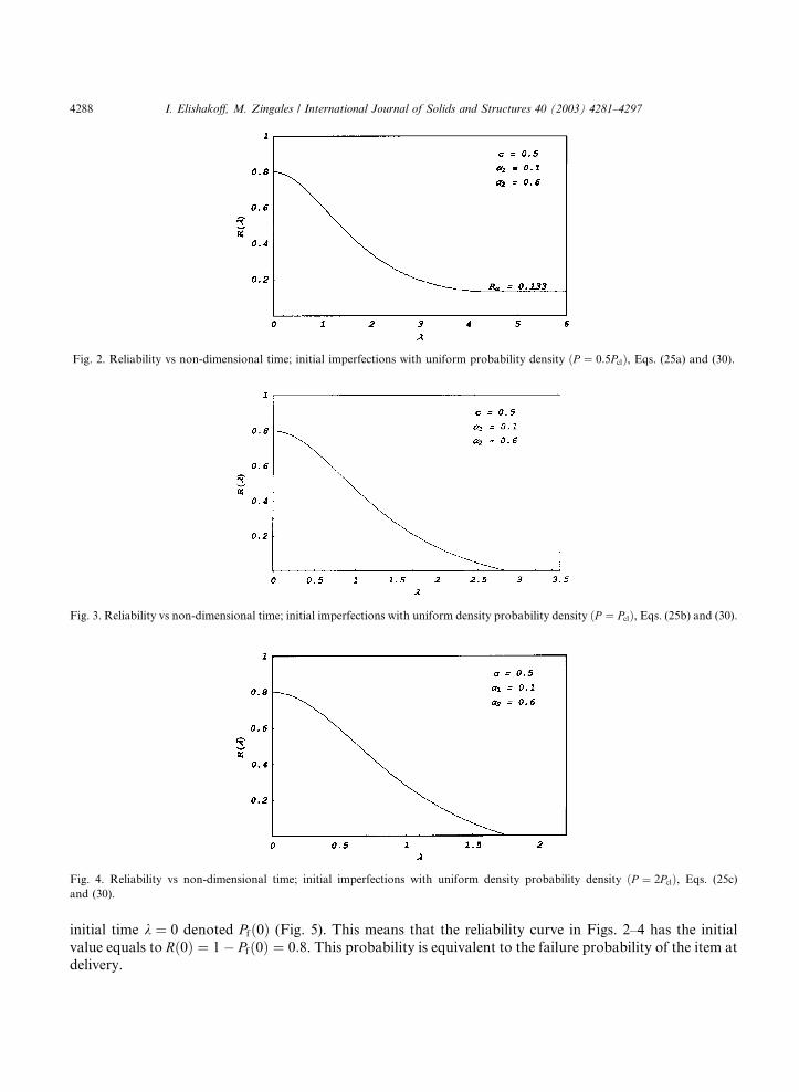
Fig. 3. Reliability vs non-dimensional time; initial imperfections with uniform density probability density ðP ¼ PclÞ, Eqs. (25b) and (30).

Fig. 4. Reliability vs non-dimensional time; initial imperfections with uniform density probability density ðP ¼ 2PclÞ, Eqs. (25c)and (30).

Fig. 2. Reliability vs non-dimensional time; initial imperfections with uniform probability density ðP ¼ 0:5PclÞ, Eqs. (25a) and (30).

4288 I. Elishakoff, M. Zingales / International Journal of Solids and Structures 40 (2003) 4281–4297

initial time k ¼ 0 denoted Pfð0Þ (Fig. 5). This means that the reliability curve in Figs. 2–4 has the initial

value equals to Rð0Þ ¼ 1� Pfð0Þ ¼ 0:8. This probability is equivalent to the failure probability of the item at

delivery.

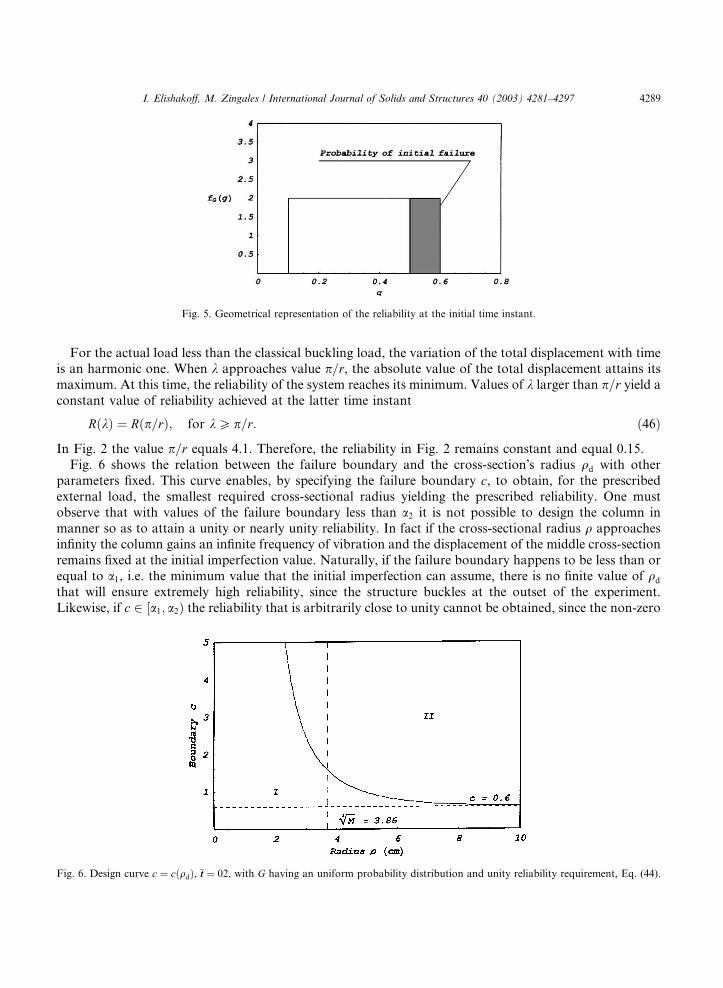
Fig. 5. Geometrical representation of the reliability at the initial time instant.

I. Elishakoff, M. Zingales / International Journal of Solids and Structures 40 (2003) 4281–4297 4289

For the actual load less than the classical buckling load, the variation of the total displacement with timeis an harmonic one. When k approaches value p=r, the absolute value of the total displacement attains its

maximum. At this time, the reliability of the system reaches its minimum. Values of k larger than p=r yield a

constant value of reliability achieved at the latter time instant

Fig. 6.

RðkÞ ¼ Rðp=rÞ; for kP p=r: ð46Þ

In Fig. 2 the value p=r equals 4.1. Therefore, the reliability in Fig. 2 remains constant and equal 0.15.

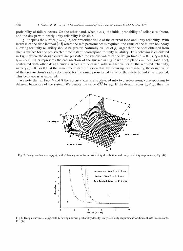
Fig. 6 shows the relation between the failure boundary and the cross-section�s radius qd with other

parameters fixed. This curve enables, by specifying the failure boundary c, to obtain, for the prescribed

external load, the smallest required cross-sectional radius yielding the prescribed reliability. One must

observe that with values of the failure boundary less than a2 it is not possible to design the column in

manner so as to attain a unity or nearly unity reliability. In fact if the cross-sectional radius q approachesinfinity the column gains an infinite frequency of vibration and the displacement of the middle cross-section

remains fixed at the initial imperfection value. Naturally, if the failure boundary happens to be less than or

equal to a1, i.e. the minimum value that the initial imperfection can assume, there is no finite value of qd

that will ensure extremely high reliability, since the structure buckles at the outset of the experiment.

Likewise, if c 2 ½a1; a2Þ the reliability that is arbitrarily close to unity cannot be obtained, since the non-zero

Design curve c ¼ cðqdÞ, �tt ¼ 02, with G having an uniform probability distribution and unity reliability requirement, Eq. (44).

4290 I. Elishakoff, M. Zingales / International Journal of Solids and Structures 40 (2003) 4281–4297

probability of failure occurs. On the other hand, when cP a2 the initial probability of collapse is absent,

and the design with nearly unity reliability is feasible.

Fig. 7 depicts the surface q ¼ qðc; tÞ for prescribed value of the external load and unity reliability. With

increase of the time interval ½0;�tt where the safe performance is required, the value of the failure boundaryallowing for unity reliability should be greater. Naturally, values of qd larger than the ones obtained from

such a surface for the pre-selected time instant t correspond to unity reliability. This behavior is elucidated

in Fig. 8 where the design curves are presented for various values of the design times t1 ¼ 0:3 s, t2 ¼ 0:8 s,

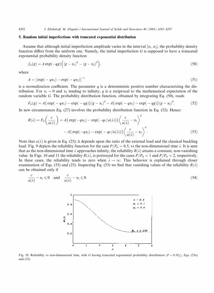
t3 ¼ 2:5 s. Fig. 9 represents the cross-section of the surface in Fig. 7 with the plane �tt ¼ 0:5 s (solid line),

contrasted with other design curves, which are obtained with smaller values of the required reliability,

namely rc ¼ 0:9 or 0.8, at the same time instant. It is seen that, by requiring less reliability, the design value

of the cross-section�s radius decreases, for the same, pre-selected value of the safety bound c, as expected.This behavior is as expected.

We note that in Figs. 6 and 8 the abscissa axes are subdivided into two sub-regions, corresponding to

different behaviors of the system. We denote the valueffiffiffiffiffiM4

pby qdc. If the design radius qd 6 qdc then the

Fig. 7. Design surface c ¼ cðqd; tÞ, with G having an uniform probability distribution and unity reliability requirement, Eq. (44).

Fig. 8. Design curves c ¼ cðqdÞ, with G having uniform probability density, unity reliability requirement for different safe time instants,

Eq. (44).

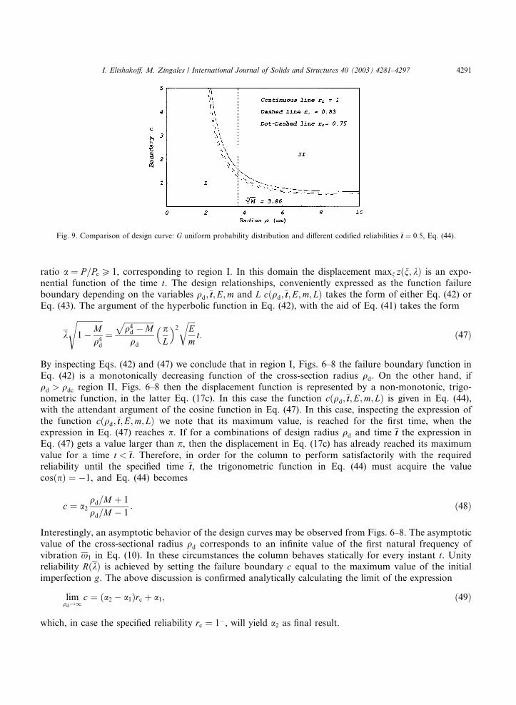
Fig. 9. Comparison of design curve: G uniform probability distribution and different codified reliabilities �tt ¼ 0:5, Eq. (44).

I. Elishakoff, M. Zingales / International Journal of Solids and Structures 40 (2003) 4281–4297 4291

ratio a ¼ P=Pc P 1, corresponding to region I. In this domain the displacement maxn zðn; kÞ is an expo-nential function of the time t. The design relationships, conveniently expressed as the function failure

boundary depending on the variables qd;�tt;E;m and L cðqd;�tt;E;m; LÞ takes the form of either Eq. (42) or

Eq. (43). The argument of the hyperbolic function in Eq. (42), with the aid of Eq. (41) takes the form

k

ffiffiffiffiffiffiffiffiffiffiffiffiffi1�M

q4d

s¼

ffiffiffiffiffiffiffiffiffiffiffiffiffiffiffiq4d �M

pqd

pL

� �2 ffiffiffiffiEm

rt: ð47Þ

By inspecting Eqs. (42) and (47) we conclude that in region I, Figs. 6–8 the failure boundary function in

Eq. (42) is a monotonically decreasing function of the cross-section radius qd. On the other hand, if

qd > qdc region II, Figs. 6–8 then the displacement function is represented by a non-monotonic, trigo-nometric function, in the latter Eq. (17c). In this case the function cðqd;�tt;E;m; LÞ is given in Eq. (44),

with the attendant argument of the cosine function in Eq. (47). In this case, inspecting the expression of

the function cðqd;�tt;E;m; LÞ we note that its maximum value, is reached for the first time, when the

expression in Eq. (47) reaches p. If for a combinations of design radius qd and time �tt the expression in

Eq. (47) gets a value larger than p, then the displacement in Eq. (17c) has already reached its maximum

value for a time t < �tt. Therefore, in order for the column to perform satisfactorily with the required

reliability until the specified time �tt, the trigonometric function in Eq. (44) must acquire the value

cosðpÞ ¼ �1, and Eq. (44) becomes

c ¼ a2

qd=M þ 1

qd=M � 1: ð48Þ

Interestingly, an asymptotic behavior of the design curves may be observed from Figs. 6–8. The asymptotic

value of the cross-sectional radius qd corresponds to an infinite value of the first natural frequency of

vibration x1 in Eq. (10). In these circumstances the column behaves statically for every instant t. Unityreliability RðkÞ is achieved by setting the failure boundary c equal to the maximum value of the initial

imperfection g. The above discussion is confirmed analytically calculating the limit of the expression

limqd!1

c ¼ ða2 � a1Þrc þ a1; ð49Þ

which, in case the specified reliability rc ¼ 1�, will yield a2 as final result.

4292 I. Elishakoff, M. Zingales / International Journal of Solids and Structures 40 (2003) 4281–4297

5. Random initial imperfections with truncated exponential distribution

Assume that although initial imperfection amplitude varies in the interval ½a1; a2, the probability density

function differs from the uniform one. Namely, the initial imperfection G is supposed to have a truncatedexponential probability density function

Fig. 1

and (5

fGðgÞ ¼ A expð�qgÞ hg�

� a1i0 � hg � a2i0�; ð50Þ

where

A ¼ expð½ � qa1Þ � expð � qa2Þ�1 ð51Þ

is a normalization coefficient. The parameter q is a deterministic positive number characterizing the dis-

tribution. For a1 ¼ 0 and a2 tending to infinity, q is a reciprocal to the mathematical expectation of the

random variable G. The probability distribution function, obtained by integrating Eq. (50), reads

FGðgÞ ¼ A expðf � qa1Þ � expð � qgÞghg � a1i0 � A expðf � qa2Þ � expð � qgÞghg � a2i0: ð52Þ

In new circumstances Eq. (27) involves the probability distribution function in Eq. (52). Hence:

RðkÞ ¼ FGc

aðkÞ

�¼ A expðf �qa1Þ � expð�qc=aðkÞÞg c

aðkÞ

�� a1

�0

� A expðf �qa2Þ � expð � qc=aðkÞÞg caðkÞ

�� a2

�0

: ð53Þ

Note that aðkÞ is given in Eq. (25); it depends upon the ratio of the external load and the classical buckling

load. Fig. 9 depicts the reliability function for the case P=Pcl ¼ 0:5, vs the non-dimensional time k. It is seenthat as the non-dimensional time k approaches infinity, the reliability RðkÞ attains a constant, non-vanishingvalue. In Figs. 10 and 11 the reliability RðkÞ, is portrayed for the cases P=Pcl ¼ 1 and P=Pcl ¼ 2, respectively.

In these cases, the reliability tends to zero when k ! 1. This behavior is explained through closer

examination of Eqs. (53) and (25). Inspecting Eq. (53) we find that vanishing values of the reliability RðkÞcan be obtained only if

caðkÞ � a1 6 0 and

caðkÞ � a2 6 0: ð54Þ

0. Reliability vs non-dimensional time, with G having truncated exponential probability distribution ðP ¼ 0:5PclÞ, Eqs. (25a)2).

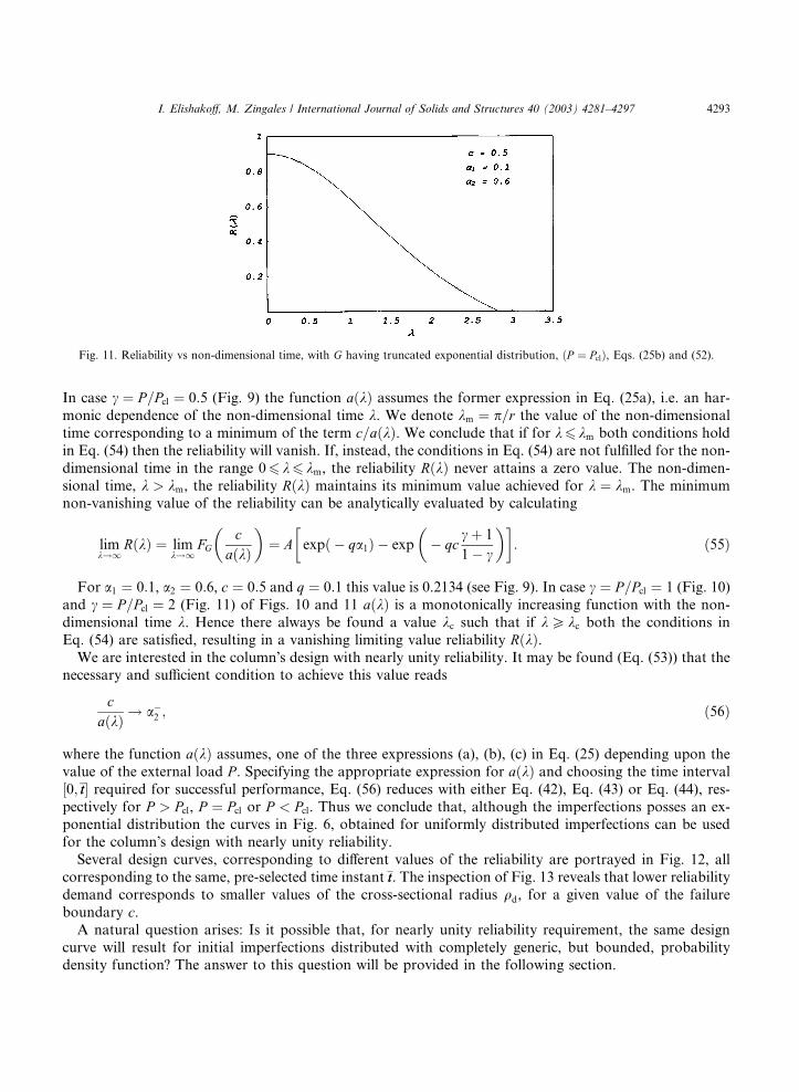
Fig. 11. Reliability vs non-dimensional time, with G having truncated exponential distribution, ðP ¼ PclÞ, Eqs. (25b) and (52).

I. Elishakoff, M. Zingales / International Journal of Solids and Structures 40 (2003) 4281–4297 4293

In case c ¼ P=Pcl ¼ 0:5 (Fig. 9) the function aðkÞ assumes the former expression in Eq. (25a), i.e. an har-

monic dependence of the non-dimensional time k. We denote km ¼ p=r the value of the non-dimensional

time corresponding to a minimum of the term c=aðkÞ. We conclude that if for k6 km both conditions hold

in Eq. (54) then the reliability will vanish. If, instead, the conditions in Eq. (54) are not fulfilled for the non-

dimensional time in the range 06 k6 km, the reliability RðkÞ never attains a zero value. The non-dimen-

sional time, k > km, the reliability RðkÞ maintains its minimum value achieved for k ¼ km. The minimumnon-vanishing value of the reliability can be analytically evaluated by calculating

limk!1

RðkÞ ¼ limk!1

FGc

aðkÞ

�¼ A expð

�� qa1Þ � exp

� qc

c þ 1

1� c

� : ð55Þ

For a1 ¼ 0:1, a2 ¼ 0:6, c ¼ 0:5 and q ¼ 0:1 this value is 0.2134 (see Fig. 9). In case c ¼ P=Pcl ¼ 1 (Fig. 10)

and c ¼ P=Pcl ¼ 2 (Fig. 11) of Figs. 10 and 11 aðkÞ is a monotonically increasing function with the non-

dimensional time k. Hence there always be found a value kc such that if k P kc both the conditions in

Eq. (54) are satisfied, resulting in a vanishing limiting value reliability RðkÞ.We are interested in the column�s design with nearly unity reliability. It may be found (Eq. (53)) that the

necessary and sufficient condition to achieve this value reads

caðkÞ ! a�

2 ; ð56Þ

where the function aðkÞ assumes, one of the three expressions (a), (b), (c) in Eq. (25) depending upon the

value of the external load P . Specifying the appropriate expression for aðkÞ and choosing the time interval

½0;�tt required for successful performance, Eq. (56) reduces with either Eq. (42), Eq. (43) or Eq. (44), res-

pectively for P > Pcl, P ¼ Pcl or P < Pcl. Thus we conclude that, although the imperfections posses an ex-ponential distribution the curves in Fig. 6, obtained for uniformly distributed imperfections can be used

for the column�s design with nearly unity reliability.

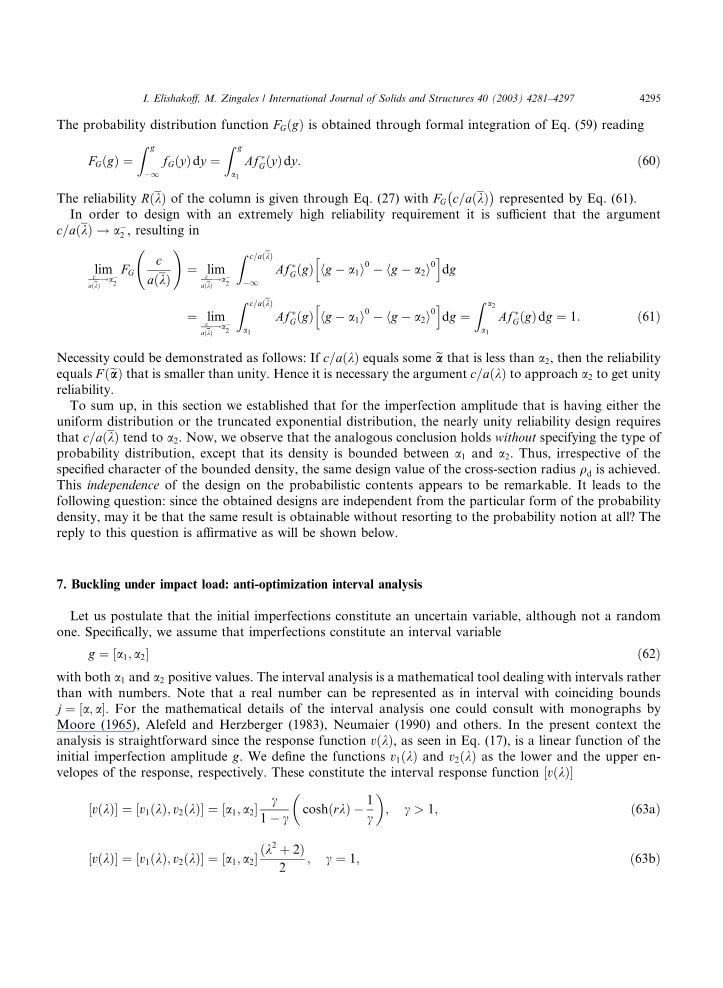
Several design curves, corresponding to different values of the reliability are portrayed in Fig. 12, all

corresponding to the same, pre-selected time instant�tt. The inspection of Fig. 13 reveals that lower reliability

demand corresponds to smaller values of the cross-sectional radius qd, for a given value of the failure

boundary c.A natural question arises: Is it possible that, for nearly unity reliability requirement, the same design

curve will result for initial imperfections distributed with completely generic, but bounded, probabilitydensity function? The answer to this question will be provided in the following section.

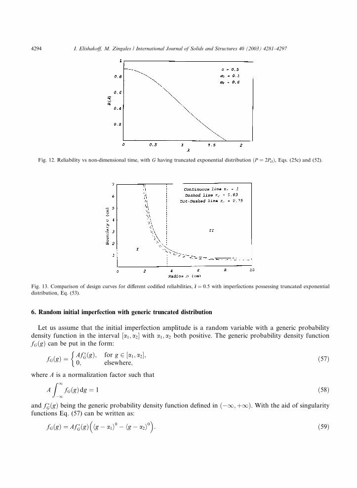
Fig. 13. Comparison of design curves for different codified reliabilities, �tt ¼ 0:5 with imperfections possessing truncated exponential

distribution, Eq. (53).

Fig. 12. Reliability vs non-dimensional time, with G having truncated exponential distribution ðP ¼ 2PclÞ, Eqs. (25c) and (52).

4294 I. Elishakoff, M. Zingales / International Journal of Solids and Structures 40 (2003) 4281–4297

6. Random initial imperfection with generic truncated distribution

Let us assume that the initial imperfection amplitude is a random variable with a generic probability

density function in the interval ½a1; a2 with a1; a2 both positive. The generic probability density function

fGðgÞ can be put in the form:

fGðgÞ ¼Af �

GðgÞ; for g 2 ½a1; a2;0; elsewhere;

�ð57Þ

where A is a normalization factor such that

AZ 1

�1fGðgÞdg ¼ 1 ð58Þ

and f �GðgÞ being the generic probability density function defined in ð�1;þ1Þ. With the aid of singularity

functions Eq. (57) can be written as:

fGðgÞ ¼ Af �GðgÞ hg

�� a1i0 � hg � a2i0

�: ð59Þ

I. Elishakoff, M. Zingales / International Journal of Solids and Structures 40 (2003) 4281–4297 4295

The probability distribution function FGðgÞ is obtained through formal integration of Eq. (59) reading

FGðgÞ ¼Z g

�1fGðyÞdy ¼

Z g

a1

Af �GðyÞdy: ð60Þ

�

The reliability RðkÞ of the column is given through Eq. (27) with FG c=aðkÞ represented by Eq. (61).

In order to design with an extremely high reliability requirement it is sufficient that the argument

c=aðkÞ ! a�2 , resulting in

limc

aðkÞ!a�

2

FGc

aðkÞ

!¼ lim

caðkÞ

!a�2

Z c=aðkÞ

�1Af �

GðgÞ hgh

� a1i0 � hg � a2i0idg

¼ limc

aðkÞ!a�

2

Z c=aðkÞ

a1

Af �GðgÞ hg

h� a1i0 � hg � a2i0

idg ¼

Z a2

a1

Af �GðgÞdg ¼ 1: ð61Þ

Necessity could be demonstrated as follows: If c=aðkÞ equals some eaa that is less than a2, then the reliability

equals F ðeaaÞ that is smaller than unity. Hence it is necessary the argument c=aðkÞ to approach a2 to get unity

reliability.

To sum up, in this section we established that for the imperfection amplitude that is having either the

uniform distribution or the truncated exponential distribution, the nearly unity reliability design requires

that c=aðkÞ tend to a2. Now, we observe that the analogous conclusion holds without specifying the type of

probability distribution, except that its density is bounded between a1 and a2. Thus, irrespective of thespecified character of the bounded density, the same design value of the cross-section radius qd is achieved.

This independence of the design on the probabilistic contents appears to be remarkable. It leads to the

following question: since the obtained designs are independent from the particular form of the probability

density, may it be that the same result is obtainable without resorting to the probability notion at all? The

reply to this question is affirmative as will be shown below.

7. Buckling under impact load: anti-optimization interval analysis

Let us postulate that the initial imperfections constitute an uncertain variable, although not a random

one. Specifically, we assume that imperfections constitute an interval variable

g ¼ ½a1; a2 ð62Þ

with both a1 and a2 positive values. The interval analysis is a mathematical tool dealing with intervals rather

than with numbers. Note that a real number can be represented as in interval with coinciding boundsj ¼ ½a; a. For the mathematical details of the interval analysis one could consult with monographs by

Moore (1965), Alefeld and Herzberger (1983), Neumaier (1990) and others. In the present context the

analysis is straightforward since the response function vðkÞ, as seen in Eq. (17), is a linear function of the

initial imperfection amplitude g. We define the functions v1ðkÞ and v2ðkÞ as the lower and the upper en-

velopes of the response, respectively. These constitute the interval response function ½vðkÞ

½vðkÞ ¼ ½v1ðkÞ; v2ðkÞ ¼ ½a1; a2c

1� ccoshðrkÞ

� 1

c

�; c > 1; ð63aÞ

½vðkÞ ¼ ½v1ðkÞ; v2ðkÞ ¼ ½a1; a2ðk2 þ 2Þ

2; c ¼ 1; ð63bÞ

4296 I. Elishakoff, M. Zingales / International Journal of Solids and Structures 40 (2003) 4281–4297

½vðkÞ ¼ ½v1ðkÞ; v2ðkÞ ¼ ½a1; a2c

c � 1cosðrkÞ

� 1

c

�; c < 1: ð63cÞ

Inspection of Eq. (63) reveals that the interval displacement function of non-dimensional time k is

represented as a product of an interval variable ½a1; a2 by a deterministic function aðkÞ defined in Eq. (25).

In order to design the column, i.e. to guarantee its successful performance until the pre-selected time�tt, or itsnon-dimensional counterpart k, it is necessary and sufficient to bound the largest possible displacement to

satisfy the inequality

v2ðkÞ6 c; ð64Þ

where c is the failure boundary. Bearing in mind Eq. (63) in conjunction with Eq. (25) we get

c6 aðkÞa2: ð65Þ

We note that the design condition in Eq. (65) coincides formally with Eq. (54) when the required reliability

approaches unity from below. This proves the equivalence between the results furnished by interval analysisand probabilistic one when rc attains values extremely close to unity.

8. Conclusions

A one-dimensional impact-buckling problem was studied in this paper in order to contrast the proba-

bilistic and non-probabilistic analyses of uncertainty. Simplicity of the example allows us not to loose sightof the ‘‘forest amongst the trees’’ of analytical and numerical derivations. In particular, this example

illustrates that the probabilistic analysis and the non-probabilistic, interval analyses are compatible with

each other. In probabilistic analysis one postulates the knowledge of the probability density function.

Often, such an information is unavailable. To model this situation we constructed two alternative models of

probability density, tough utilizing a random variable with either uniform or non-uniform truncated

density. Both yielded the same value for the design variable. This result lead to the general conclusion, that

irrespective of the density involved, except of it extending between the lower possible value a1 and the upper

possible one a2, the same designs will follow. This could be interpreted as ‘‘good news’’ for the probabilists.Researchers in the field of stochasticity could argue that the unavailability of the probability density, except

that the information on its boundedness may be immaterial. Thus any assumption on the probability

density will be equally efficient. If, however, the experimental data is available, then the appropriate density

should be utilized. We maintain that a design point at the bound of the distribution provides a ‘‘near unity’’

probability. This seems blatantly transparent. Yet this fact appears not to be emphasized by the proba-

bilistic analysts. Even though the of the probability density function is not needed in the interval analysis,

one must face the issue on how to properly define bounds. Except in special cases where there exist well

defined bounds, the selection of the bounds will likely rely on a decision, perhaps based on data analysis orphysical arguments.

Remarkably, the same designs furnished by the probabilistic analysis were also obtained through the use

of the interval analysis. This suggests the following idea: since the initial imperfection is an uncertain value,

and often no data is available to justify the particular choice of the density, why do not to employ the

simplest possible approach? Interval mathematics is indeed such a method. Although in this particular case

interval analysis may appear simple, it provides with the same result as derived by more sophisticated and

algebraically lengthier probabilistic analysis. It is concluded, therefore, due to engineering pragmatism, that

in some circumstances the non-probabilistic analysis of uncertainty may be preferable to probabilistic one,since it leads to the same results, as the probabilistic analysis, in a much simpler manner.

I. Elishakoff, M. Zingales / International Journal of Solids and Structures 40 (2003) 4281–4297 4297

Acknowledgements

This study has been supported by the N.A.S.A. Langley Research Center (I.E.) and the Italian Ministry

of Science and Technological Research (M.Z.). This financial support is gratefully appreciated.

References

Alefeld, G., Herzberger, J., 1983. Introduction to Interval Computations. Academic Press, New York.

Chernousko, F.E.L., 1994. State Estimation of Dynamic Systems. CRC Press, Boca Raton.

Elishakoff, I., 1978. Axial impact buckling of columns with random initial imperfections. Journal of Applied Mechanics 45, 361–365.

Elishakoff, I., Ben-Haim, Y., 1990. Dynamics of thin cylindrical shell under impact with limited deterministic informations on its initial

imperfections. Structural Safety 8, 103–112.

Elishakoff, I., Li, Q., 1999. How to combine probabilistic and anti-optimization methods? Whys and hows in uncertainty modeling

(probability, fuzziness and anti-optimization). In: Elishakoff, I. (Ed.), CISM Courses and Lectures. Springer-Verlag, Wien, New

York, pp. 319–339.

Elishakoff, I., Cai, G.Q., Starnes Jr., J.H., 1994. Nonlinear buckling of columns with initial imperfection via stochastic and non-

stochastic, convex models. International Journal of Non-Linear Mechanics 29, 71–82.

Hoff, N.J., 1965. In: Herrmann, G. (Ed.), Dynamic Stability of Structures. Pergamon Press, New York, pp. 7–44.

Kim, Yu.V., Ovseyevich, A.I., Reshetnyak, Yu.N., 1993. Comparison of stochastic and guaranteed approaches to the estimation of the

state of dynamic systems. Journal of Computer and System Sciences International 31 (6), 56–64.

Kurzhanski, A.B., 1977. Control and Observation Under Conditions of Uncertainty. Nauka, Moscow (in Russian).

Moore, R., 1965. Methods and Applications of Interval Analysis. SIAM, Philadelphia.

Neumaier, A., 1990. Interval Methods for System of Equations. Cambridge University Press, New York.