1.5 probabilistic reasoning
TRANSCRIPT
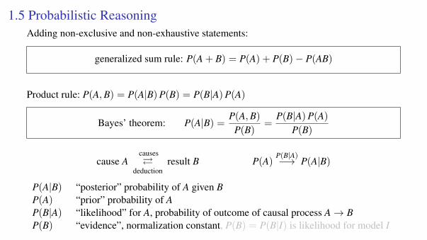
1.5 Probabilistic ReasoningAdding non-exclusive and non-exhaustive statements:
generalized sum rule: P(A + B) = P(A) + P(B)− P(AB)
Product rule: P(A,B) = P(A|B) P(B) = P(B|A) P(A)
Bayes’ theorem: P(A|B) =P(A,B)
P(B)=
P(B|A) P(A)
P(B)
cause Acauses
deductionresult B P(A)
P(B|A)−→ P(A|B)
P(A|B) “posterior” probability of A given BP(A) “prior” probability of AP(B|A) “likelihood” for A, probability of outcome of causal process A→ BP(B) “evidence”, normalization constant, P(B) = P(B|I) is likelihood for model I
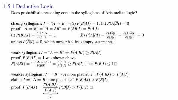
1.5.1 Deductive LogicDoes probabilistic reasoning contain the syllogisms of Aristotelian logic?
strong syllogism: I = “A⇒ B”⇒(i) P(B|AI) = 1, (ii) P(A|BI) = 0proof: “A⇒ B” = “A = AB”⇒ P(AB|I) = P(A|I)(i) P(B|AI) = P(AB|I)
P(A|I) = 1, (ii) P(A|BI) = P(AB|I)P(B|I) = P(ABB|I)
P(B|I) = 0
unless P(B|I) = 0, which turns r.h.s. into empty statement
weak syllogism: I = “A⇒ B”⇒ P(A|BI) ≥ P(A|I)proof: P(B|AI) = 1 was shown aboveP(A|BI) = P(B|AI) P(A|I)
P(B|I) = P(A|I)P(B|I) ≥ P(A|I) since P(B|I) ≤ 1
weaker syllogism: J = “B⇒ A more plausible”, P(A|BJ) > P(A|J)claim: J ⇒ “A⇒ B more plausible”, P(B|AJ) > P(B|J)
proof: P(B|AJ) =P(A|BJ)
P(A|J)︸ ︷︷ ︸>1
P(B|J) > P(B|J)
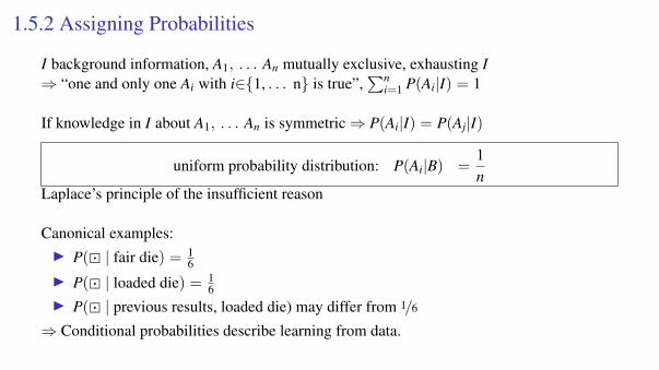
1.5.2 Assigning Probabilities
I background information, A1, . . . An mutually exclusive, exhausting I⇒ “one and only one Ai with i∈1, . . . n is true”,
∑ni=1 P(Ai|I) = 1
If knowledge in I about A1, . . . An is symmetric⇒ P(Ai|I) = P(Aj|I)
uniform probability distribution: P(Ai|B) =1n
Laplace’s principle of the insufficient reason
Canonical examples:I P( | fair die) = 1
6
I P( | loaded die) = 16
I P( | previous results, loaded die) may differ from 1/6
⇒ Conditional probabilities describe learning from data.
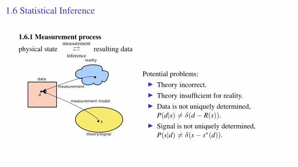
1.6 Statistical Inference
1.6.1 Measurement process
physical statemeasurement
inferenceresulting data
reality
data
theory/signal
s
d
measurement
measurement model
Potential problems:I Theory incorrect.I Theory insufficient for reality.I Data is not uniquely determined,
P(d|s) 6= δ(d − R(s)).I Signal is not uniquely determined,
P(s|d) 6= δ(s− s∗(d)).
1.6.2 Bayesian InferenceI= background information: on signal s, on measurement yielding data dI assumed impicitly in the following, P(s) := P(s|I) etc.
Bayes’ theorem: P(s|d) =P(d, s)
P(d)=
P(d|s)P(d)
P(s)
Sloppy notation: P(s) = P(svar = sval|I), svar unknown variable, sval concrete value
Observations:I Joint probability P(d, s) decomposed in likelihood and priorI Prior P(s) summarizes knowledge on s prior to measurment
I Likelihood P(d|s) describes measurement process, updates prior, P(s)P(d|s)−→ P(s|d)
I Evidence P(d) =∑
s P(d, s) normalizes posterior∑s
P(s|d) =∑
s
P(d, s)P(d)
=
∑s P(d, s)∑
s′ P(d, s′)= 1
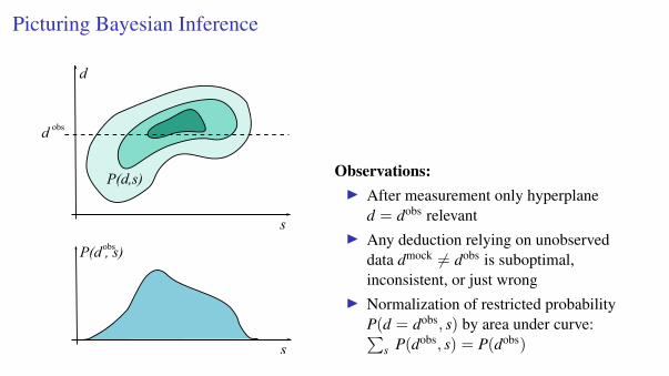
Picturing Bayesian Inference
s
d
s
P(d , s)
d obs
obs
P(d,s) Observations:I After measurement only hyperplane
d = dobs relevantI Any deduction relying on unobserved
data dmock 6= dobs is suboptimal,inconsistent, or just wrong
I Normalization of restricted probabilityP(d = dobs, s) by area under curve:∑
s P(dobs, s) = P(dobs)
1.7 Coin tossing
1.7.1 Recognizing the unfair coinI1 = “Outcome of coin tosses stored in data d = (d1, d2, . . .),di ∈ head, tail := 1, 0 of ith toss, d(n) = (d1, . . . dn) = data up to toss n”
Question 1: What is our knowledge on d(1) = (d1) given I1?Due to symmetry in knowledge: P(d1 = 0|I1) = P(d1 = 1|I1) = 1/2
Question 2: What is our knowledge about dn+1 given d(n), I1?
P(dn+1|d(n), I1) =P(d(n+1)|I1)
P(d(n)|I1)with d(n+1) = (dn+1, d(n+1))
I1 symmetric w.r.t. 2n possible sequences d(n) ∈ 0, 1n of length n⇒ P(d(n)|I1) = 2−n
P(dn+1|d(n), I1) =2−n−1
2−n =12
Statistical Independence
Given I1, the data d(n) contains no useful information on dn+1. What did we miss?It seems I1 ⇒ “All tosses are statistically independent of each other.”
A and B statistically independent under C⇔ P(A|BC) = P(A|C)⇒ P(AB|C) = P(A|BC) P(B|C) = P(A|C) P(B|C)
Additional information I2 = “Tosses done with same coin, which might be loaded,meaning heads occur with frequency f ”∃f ∈ [0, 1] : ∀i ∈ N : P(di = 1|f , I1, I2) = f , I = I1I2
P(di|f , I) =
f di = 11− f di = 0
= f di (1− f )1−di
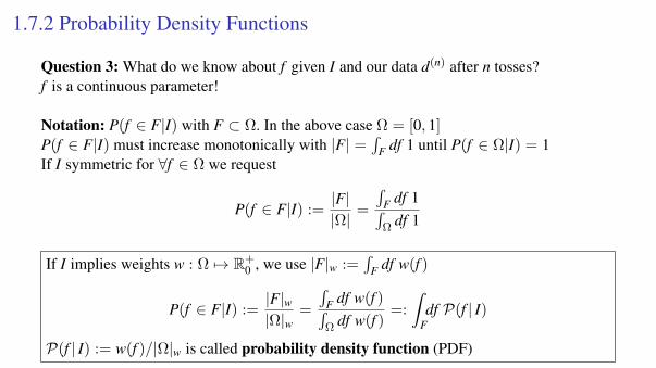
1.7.2 Probability Density Functions
Question 3: What do we know about f given I and our data d(n) after n tosses?f is a continuous parameter!
Notation: P(f ∈ F|I) with F ⊂ Ω. In the above case Ω = [0, 1]P(f ∈ F|I) must increase monotonically with |F| =
´F df 1 until P(f ∈ Ω|I) = 1
If I symmetric for ∀f ∈ Ω we request
P(f ∈ F|I) :=|F||Ω|
=
´F df 1´Ω df 1
If I implies weights w : Ω 7→ R+0 , we use |F|w :=
´F df w(f )
P(f ∈ F|I) :=|F|w|Ω|w
=
´F df w(f )´Ω df w(f )
=:
ˆFdf P(f | I)
P(f | I) := w(f )/|Ω|w is called probability density function (PDF)
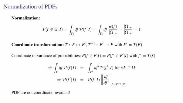
Normalization of PDFs
Normalization:
P(f ∈ Ω| I) =
ˆΩ
df P(f | I) =
ˆΩ
dfw(f )
|Ω|w=|Ω|w|Ω|w
= 1
Coordinate transformation: T : F 7→ F′, T−1 : F′ 7→ F with F′ = T(F)
Coordinate in-variance of probabilities: P(f ∈ F|I) = P(f ′ ∈ F′|I) with f ′ = T(f )
⇒ˆ
Fdf P(f | I) =
ˆF′
df ′ P(f ′| I) for ∀F ⊂ Ω
⇒ P(f ′| I) = P(f | I)∥∥∥∥ df
df ′
∥∥∥∥f =T−1(f ′)
PDF are not coordinate invariant!
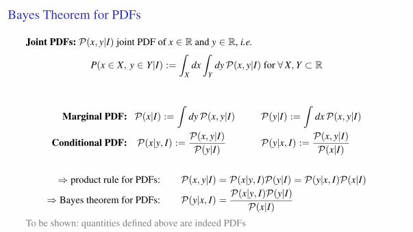
Bayes Theorem for PDFs
Joint PDFs: P(x, y|I) joint PDF of x ∈ R and y ∈ R, i.e.
P(x ∈ X, y ∈ Y|I) :=
ˆX
dxˆ
YdyP(x, y|I) for ∀X,Y ⊂ R
Marginal PDF: P(x|I) :=
ˆdyP(x, y|I) P(y|I) :=
ˆdxP(x, y|I)
Conditional PDF: P(x|y, I) :=P(x, y|I)P(y|I)
P(y|x, I) :=P(x, y|I)P(x|I)
⇒ product rule for PDFs: P(x, y|I) = P(x|y, I)P(y|I) = P(y|x, I)P(x|I)
⇒ Bayes theorem for PDFs: P(y|x, I) =P(x|y, I)P(y|I)P(x|I)
To be shown: quantities defined above are indeed PDFs
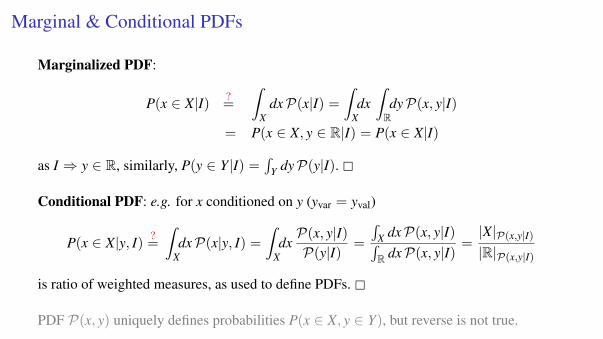
Marginal & Conditional PDFs
Marginalized PDF:
P(x ∈ X|I) ?=
ˆX
dxP(x|I) =
ˆXdxˆRdyP(x, y|I)
= P(x ∈ X, y ∈ R|I) = P(x ∈ X|I)
as I ⇒ y ∈ R, similarly, P(y ∈ Y|I) =´
Y dyP(y|I).
Conditional PDF: e.g. for x conditioned on y (yvar = yval)
P(x ∈ X|y, I) ?=
ˆXdxP(x|y, I) =
ˆXdxP(x, y|I)P(y|I)
=
´X dxP(x, y|I)´R dxP(x, y|I)
=|X|P(x,y|I)
|R|P(x,y|I)
is ratio of weighted measures, as used to define PDFs.
PDF P(x, y) uniquely defines probabilities P(x ∈ X, y ∈ Y), but reverse is not true.
1.7.3 Infering the coin load
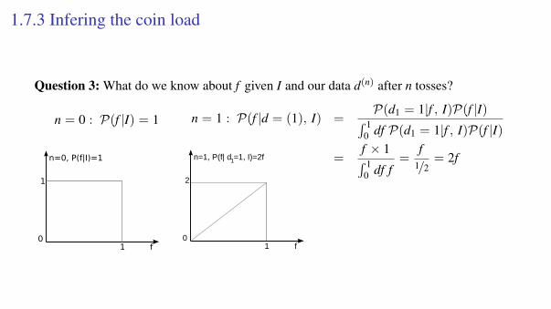
Question 3: What do we know about f given I and our data d(n) after n tosses?
n = 0 : P(f |I) = 1
n=0, P(f|I)=1
1
10
f
n = 1 : P(f |d = (1), I) =P(d1 = 1|f , I)P(f |I)´ 1
0 df P(d1 = 1|f , I)P(f |I)
=f × 1´ 10 df f
=f
1/2= 2fn=1, P(f| d =1, I)=2f
2
10
f
1
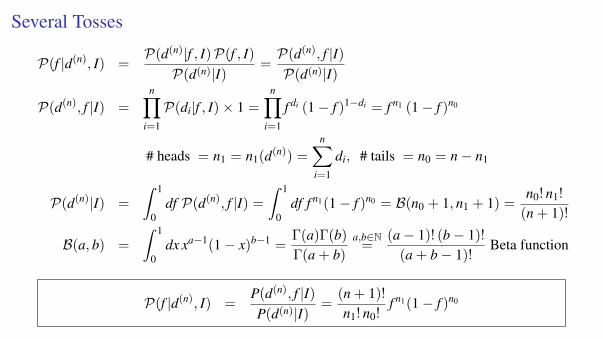
Several Tosses
P(f |d(n), I) =P(d(n)|f , I)P(f , I)P(d(n)|I)
=P(d(n), f |I)P(d(n)|I)
P(d(n), f |I) =
n∏i=1
P(di|f , I)× 1 =
n∏i=1
f di (1− f )1−di = f n1 (1− f )n0
# heads = n1 = n1(d(n)) =
n∑i=1
di, # tails = n0 = n− n1
P(d(n)|I) =
ˆ 1
0df P(d(n), f |I) =
ˆ 1
0df f n1(1− f )n0 = B(n0 + 1, n1 + 1) =
n0! n1!
(n + 1)!
B(a, b) =
ˆ 1
0dx xa−1(1− x)b−1 =
Γ(a)Γ(b)
Γ(a + b)
a,b∈N=
(a− 1)! (b− 1)!
(a + b− 1)!Beta function
P(f |d(n), I) =P(d(n), f |I)P(d(n)|I)
=(n + 1)!
n1! n0!f n1(1− f )n0
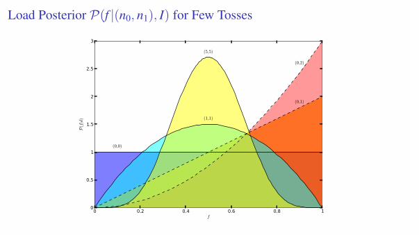
Load Posterior P(f |(n0, n1), I) for Few Tosses
0 0.2 0.4 0.6 0.8 1f
0
0.5
1
1.5
2
2.5
3
P(f|d)
(0,0)
(0,1)
(0,2)
(1,1)
(5,5)
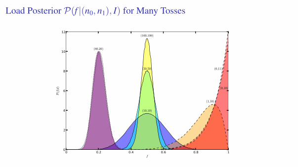
Load Posterior P(f |(n0, n1), I) for Many Tosses
0 0.2 0.4 0.6 0.8 1f
0
2
4
6
8
10
12
P(f|d)
(10,10)
(50,50)
(100,100)
(80,20)
(0,11)
(1,10)
(0,10)
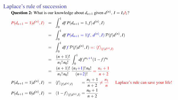
Laplace’s rule of successionQuestion 2: What is our knowledge about dn+1 given d(n), I = I1I2?
P(dn+1 = 1|d(n), I) =
ˆ 1
0df P(dn+1 = 1, f | d(n), I)
=
ˆ 1
0df P(dn+1 = 1|f , d(n), I)P(f |d(n), I)
=
ˆ 1
0df f P(f |d(n), I) =: 〈f 〉(f |d(n),I)
=(n + 1)!
n1! n0!
ˆ 1
0df f n1+1(1− f )n0
=(n + 1)!
n1! n0!
(n1+1)! n0!
(n+2)!=
n1 + 1n + 2
P(dn+1 = 1|d(n), I) = 〈f 〉(f |d(n),I) =n1 + 1n + 2
6= n1
nLaplace’s rule can save your life!
P(dn+1 = 0|d(n), I) = 〈1− f 〉(f |d(n),I) =n0 + 1n + 2
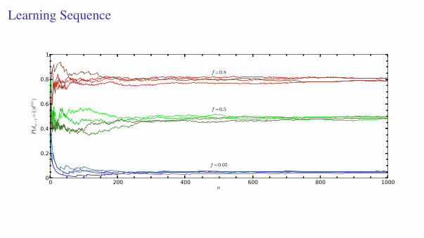
Learning Sequence
0 200 400 600 800 1000n
0
0.2
0.4
0.6
0.8
1
P(dn
+1=
1|d
(n))
f=0.8
f=0.5
f=0.05
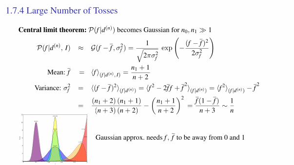
1.7.4 Large Number of Tosses
Central limit theorem: P(f |d(n)) becomes Gaussian for n0, n1 1
P(f |d(n), I) ≈ G(f − f , σ2f ) =
1√2πσ2
f
exp
(−(f − f )2
2σ2f
)
Mean: f = 〈f 〉(f |d(n), I) =n1 + 1n + 2
Variance: σ2f = 〈(f − f )2〉(f |d(n)) = 〈f 2 − 2f f + f 2〉(f |d(n)) = 〈f 2〉(f |d(n)) − f 2
=(n1 + 2) (n1 + 1)
(n + 3) (n + 2)−(
n1 + 1n + 2
)2
=f (1− f )
n + 3∼ 1
n
0 0.2 0.4 0.6 0.8 1f
0
2
4
6
8
10
12
P(f|d)
(10,10)
(50,50)
(100,100)
(80,20)
(0,11)
(1,10)
(0,10) Gaussian approx. needs f , f to be away from 0 and 1
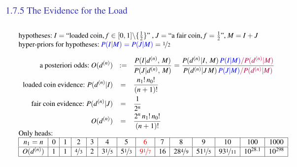
1.7.5 The Evidence for the Load
hypotheses: I = “loaded coin, f ∈ [0, 1]\ 12” , J = “a fair coin, f = 1
2 ”, M = I + Jhyper-priors for hypotheses: P(I|M) = P(J|M) = 1/2
a posteriori odds: O(d(n)) :=P(I|d(n), M)
P(J|d(n), M)=
P(d(n)|I, M) P(I|M)/P(d(n)|M)
P(d(n)|J M) P(J|M)/P(d(n)|M)
loaded coin evidence: P(d(n)|I) =n1! n0!
(n + 1)!
fair coin evidence: P(d(n)|J) =12n
O(d(n)) =2n n1! n0!
(n + 1)!Only heads:
n1 = n 0 1 2 3 4 5 6 7 8 9 10 100 1000O(d(n)) 1 1 4/3 2 31/5 51/3 91/7 16 284/9 511/5 931/11 1028.1 10298
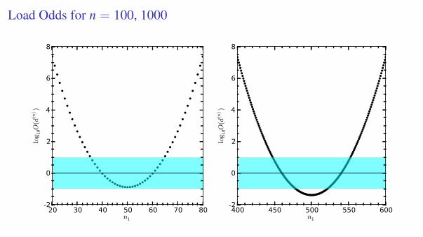
Load Odds for n = 100, 1000
20 30 40 50 60 70 80n1
-2
0
2
4
6
8
log 1
0O(d
(n))
400 450 500 550 600n1
-2
0
2
4
6
8
log 1
0O(d
(n))
1.7.6 Lessons Learned1. Probabilities described knowledge states2. Frequencies are probabilities if known, P(d = 1|f , I) = f3. Joint probability contain all relevant information4. Posterior summarizes knowledge of signal given data and model knowledge5. Evidence: Signal-marginalized joint probability, “likelihood” for model6. Background information matters: P(dn+1|d(n), I1) 6= P(dn+1|d(n), I1I2), if I2 * I1
7. Intelligence needs models: coins having a constant head frequency f8. Probability Density Functions (PDFs) serve to construct probabilies9. Learning & forgetting: Posterior changes with new data, usually sharpens thereby
10. Sufficient statistics are compressed data, giving the same information as original dataon the quantity of interest, e.g. P(f |d(n), I) = P(f |(n0, n1), I)
11. Nested models contain each other; fair coin model is included in unfair coin model12. Occam’s razor: Among competing hypotheses, the one with the fewest assumptions
should be selected.13. Uncertainty of an inferred quantity may depend on data realization
1.8 Adaptive Information Retrieval
1.8.1 Inference from adaptive data retrievalData d(n) = (d1, . . . dn) to infer signal s taken sequentially.Action ai chosen to measure di via di ← P(di|ai, s) can depend on previous data d(i−1) viadata retrieval strategy function A : d(i−1) → ai.I A predetermined strategy is independent of the prior data: A(d(i−1)) ≡ ai
irrespective of d(i−1)
I An adaptive strategy depends on the data: ∃i, d(i−1), d′(i−1) : A(d(i−1)) 6= A(d′(i−1))
New datum di depends conditionally on previous data d(i−1) through strategy A,
P(di|ai, s) = P(di|A(d(i−1)), s) = P(di|d(i−1), A, s)
Likelihood of the full data set d = d(n):
P(d|A, s) = P(dn|d(n−1), A, s) · · · P(d(1)|A, s) =
n∏i=1
P(di|d(i−1), A, s)
Different strategy B→ different actions b→ different data d′
Unknown strategy
Strategy A→ actions a, data d; strategy B→ actions b, data d′
predetermined strategy B(d(i)) ≡ ai → actions a, data d
likelihood: P(d|A, s) =
n∏i=1
P(di|A(d(i−1)), s) =
n∏i=1
P(di|ai, s)
=
n∏i=1
P(di|B(d(i−1)), s) = P(d|B, s)
posterior: P(s|d, A) =P(d|A, s)P(s|A)
P(d|A)=
P(d|A, s)P(s)P(d|A)
=P(d|A, s)P(s)∑s P(d|A, s)P(s)
=P(d|B, s)P(s)∑s P(d|B, s)P(s)
= P(s|d, B)
Used assumption: P(s|A) = P(s)
Historical Inference
Why data was taken does not matter for Bayesian inference, only how and what it was.P(s|d,A) = P(s|d,B), if strategies A, B provide identical actions for observed data,A(d(i)) = B(d(i)) = ai, and if signal is independent of strategy, P(s|A) = P(s).
Corollary: A history, a recorded sequence of interdependent observations (= actions andresulting data), is open to a Bayesian analysis without knowledge of the used strategy, butnearly useless for frequentists analysis as alternative realities are not available.
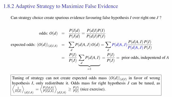
1.8.2 Adaptive Strategy to Maximize False Evidence
Can strategy choice create spurious evidence favouring false hypothesis I over right one J ?
odds: O(d) =P(I|d)
P(J|d)=
P(d|I)P(I)P(d|J)P(J)
expected odds: 〈O(d)〉(d|J,A) =∑
d
P(d|A, J) O(d) =∑
d
P(d|A, J)P(d|A, I) P(I)P(d|A, J) P(J)
=P(I)P(J)
∑d
P(d|A, I)︸ ︷︷ ︸=1
=P(I)P(J)
= prior odds, indepentend of A
Tuning of strategy can not create expected odds mass 〈O(d)〉(d|J) in favor of wronghypothesis I, only redistribute it. Odds mass for right hypothesis J can be tuned, as⟨
1O(d)
⟩(d|J,A)
=⟨
P(J|d,A)P(I|d,A)
⟩(d|J,A)
≥ P(J)P(I) (nice exercise).
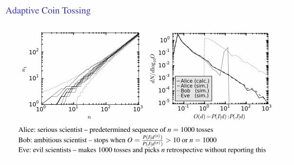
Adaptive Coin Tossing
100 101 102 103
n
100
101
102
n1
10-1 100 101 102 103
O(d) =P(I|d) :P(J|d)
10-5
10-4
10-3
10-2
10-1
100
dN/d
log
10O
Alice (calc.)Alice (sim.)Bob (sim.)Eve (sim.)
Alice: serious scientist – predetermined sequence of n = 1000 tossesBob: ambitious scientist – stops when O = P(I|d(n))
P(J|d(n))> 10 or n = 1000
Eve: evil scientists – makes 1000 tosses and picks n retrospective without reporting this

End