bimodal representation of the tropical intraseasonal oscillation
TRANSCRIPT
Bimodal representation of the tropical intraseasonal oscillation
Kazuyoshi Kikuchi • Bin Wang • Yoshiyuki Kajikawa
Received: 6 January 2011 / Accepted: 26 July 2011 / Published online: 14 August 2011
� Springer-Verlag 2011
Abstract The tropical intraseasonal oscillation (ISO)
shows distinct variability centers and propagation patterns
between boreal winter and summer. To accurately repre-
sent the state of the ISO at any particular time of a year, a
bimodal ISO index was developed. It consists of Madden-
Julian Oscillation (MJO) mode with predominant east-
ward propagation along the equator and Boreal Summer
ISO (BSISO) mode with prominent northward propaga-
tion and large variability in off-equatorial monsoon trough
regions. The spatial–temporal patterns of the MJO and
BSISO modes are identified with the extended empirical
orthogonal function analysis of 31 years (1979–2009)
OLR data for the December–February and June–August
period, respectively. The dominant mode of the ISO at
any given time can be judged by the proportions of the
OLR anomalies projected onto the two modes. The
bimodal ISO index provides objective and quantitative
measures on the annual and interannual variations of the
predominant ISO modes. It is shown that from December
to April the MJO mode dominates while from June to
October the BSISO mode dominates. May and November
are transitional months when the predominant mode
changes from one to the other. It is also shown that the
fractional variance reconstructed based on the bimodal
index is significantly higher than the counterpart recon-
structed based on the Wheeler and Hendon’s index. The
bimodal ISO index provides a reliable real time moni-
toring skill, too. The method and results provide critical
information in assessing models’ performance to repro-
duce the ISO and developing further research on pre-
dictability of the ISO and are also useful for a variety of
scientific and practical purposes.
Keywords Tropical intraseasonal oscillation � MJO �Index
1 Introduction
Tropical intraseasonal oscillation (ISO) or referred to as the
Madden-Julian oscillation (MJO) in honor of the discov-
erers (Madden and Julian 1971), characterized by the period
of 30–90 (60) days, plays a fundamental role in regulating
weather and affecting climate both in the tropics and extra
tropics. A remarkable feature, which makes the ISO so
influential in part, is its potential interactions with a variety
of spatial and temporal scales such as diurnal cycle (Chen
and Houze 1997; Ichikawa and Yasunari 2008), tropical
cyclones (Maloney and Hartmann 2000a, b; Molinari and
Vollaro 2000), El Nino (Kessler et al. 1995; Takayabu et al.
1999), annular modes (Miller et al. 2003), and monsoon
systems of Asia (Yasunari 1979; Kajikawa and Yasunari
2005), Australia (Hendon and Liebmann 1990; McBride
School of Ocean and Earth Science and Technology Contribution
Number 8213 and International Pacific Research Center Contribution
Number 798.
K. Kikuchi (&)
International Pacific Research Center, School of Ocean and
Earth Science and Technology, University of Hawaii, 1680 East
West Road, POST Bldg. 401, Manoa Honolulu, HI 96822, USA
e-mail: [email protected]
B. Wang
Department of Meteorology and International Pacific Research
Center, School of Ocean and Earth Science and Technology,
University of Hawaii, Manoa Honolulu, HI 96822, USA
Y. Kajikawa
Hydrospheric Atmospheric Research Center, Nagoya University,
Nagoya, Japan
123
Clim Dyn (2012) 38:1989–2000
DOI 10.1007/s00382-011-1159-1
et al. 1995), and North America (Higgins and Shi 2001;
Lorenz and Hartmann 2006; Moon et al. 2010).
The fundamental feature of the ISO may be best illus-
trated in a longitude-height cross sections along the equator
as in the schematic summary in their pioneering work by
Madden and Julian (1972): A planetary scale convective
anomaly consisting of mesoscale convective systems cou-
pled with large-scale circulation disturbance with the
gravest baroclinic structure moves eastward at about
5 ms-1 in the eastern hemisphere. In the western hemi-
sphere, on the other hand, upper-level circulation distur-
bance rarely coupled with convection moves eastward at a
speed of about 15–20 ms-1. The circulation disturbance is
associated with equatorial Kelvin and Rossby waves (Rui
and Wang 1990; Hendon and Salby 1994). More thorough
reviews can be found in some literatures (e.g., Madden and
Julian 1994; Lau and Waliser 2005; Zhang 2005).
Such a simple description of the ISO which moves
exclusively eastward, although is often used to describe the
major feature of the ISO, may not necessarily be appro-
priate to best document the crucial aspect of the ISO
throughout the year. There is observational evidence that
the properties of the ISO such as activity centers and
propagation patterns are strongly regulated by the annual
cycle (Madden 1986; Salby and Hendon 1994; Webster
et al. 1998; Zhang and Dong 2004). An example is given in
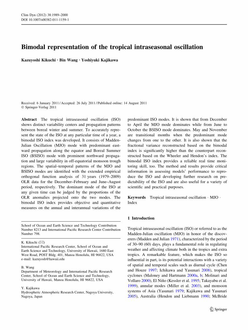
Fig. 1, which shows annual variation of the ISO propaga-
tion with emphasis on the eastern hemisphere where con-
vective systems associated with the ISO rather appear
clearly. There are two distinct propagation tendencies:
during boreal winter the organized convection associated
with the ISO shows predominantly eastward propagation
along the equator with little poleward propagation, whereas
during boreal summer it shows prominent northward
propagation over the northern Indian Ocean (and western
North Pacific, not shown) (Yasunari 1979; Knutson and
Weickmann 1987; Wang and Rui 1990) with weakened
eastward propagation. The difference in propagation
characteristic can account for the difference in the ISO
activity centers (Kemball-Cook and Wang 2001; Zhang
2005). In addition, accompanied large-scale circulation
shows rather symmetric about the equator during boreal
winter, whereas it shows asymmetric during boreal sum-
mer. Thus, the simplest model with only zonal propagation
component considered appears to be more relevant to
document the ISO behavior during boreal winter, and a
more complex model with meridional propagation com-
ponent as well as zonal propagation component considered
is more relevant to document the ISO behavior during
boreal summer.
Consideration of such annual variation of the ISO is of
critical importance for especially studies on interactions of
the ISO with a widespread variety of spatial and temporal
scales. A meticulous treatment of the ISO is the basis for
analyses of those studies, because different structures of the
ISO are expected to have different roles in weather and
climate variations. In fact, for instance, Kikuchi and Wang
(2010) showed that the winter type ISO and the summer
type ISO have different manners in which tropical cyclo-
genesis are affected over the northern Indian Ocean.
The purpose of this study is to develop an ISO index
which reflects such annual variation of the ISO. The index,
referred to as the bimodal ISO index, relies on two distinct
ISO modes, which capture the aforementioned two distinct
propagation features for the two solstice seasons. With this
method, the state of the ISO at any particular time can be
faithfully diagnosed in terms of the two ISO modes. As a
result, any ISO event can be classified into either ISO
mode, which is critical information for studies of interac-
tions of the ISO with weather and climate variations on a
wide range of timescales.
A brief review of methods used to extract ISO signals is
presented in Sect. 2. Section 3 describes the dataset and
intraseasonal time-filter used. The bimodal ISO index is
introduced in Sect. 4, which also includes some sensitivity
tests and a comparison with the Wheeler and Hendon
(2004) index. In Sect. 5, how the ISO can be represented
with the bimodal ISO index is examined. An application of
the index to real time monitoring is discussed in Sect. 6.
Section 7 summarizes this study.
TRMM 3B42 2001
mmmm
(a)
(b)
Fig. 1 Daily precipitation (tropical rainfall measuring mission prod-
uct 3B42) associated with the ISO for the year 2001. a Latitude-time
plot over the eastern Indian Ocean averaged between 80 and 100�E
and (b) longitude-time plot along the equator between 7.5�S and
7.5�N. Each red closed circles indicates major convection associated
with significant ISO events, determined by our analysis to be
introduced in Sect. 4 (see also Fig. 4), sitting around the central
Indian Ocean (90�E, 0�). Solid and dashed lines show reference phase
speed corresponding to (a) northward propagation at approximately
1–2 ms-1 and (b) eastward propagation at approximately 6 ms-1.
The solid lines are intended to represent rather apparent convection
exists
1990 K. Kikuchi et al.: Bimodal representation
123
2 A review of methods used to extract ISO signals
Before introducing the bimodal ISO index, it is worth
reviewing methods that have been used to extract ISO
signals, although majority of these methods were not
intended to construct an ISO index. A variety of methods
have been used with various degrees of complexity. Per-
haps the simplest method is to focus on an intraseasonal
fluctuation of a single variable at a particular location, and
document the ISO behavior based on that variability (e.g.,
Julian and Madden 1981; Hendon and Salby 1994), while
the most meticulous and comprehensive method is a
tracking method (Wang and Rui 1990; Jones et al. 2004) as
it is carefully designed to depict various types of convec-
tive behaviors associated with the ISO.
Between those extremes, Eigen techniques have been
widely used (Table 1). Eigen techniques provide a conve-
nient method for the description of the spatial and temporal
variability associated with the ISO in terms of empirically
derived functions (spatial patterns in general). Since the
ISO is characterized by organized convection coupled with
large-scale circulation with the gravest baroclinic structure,
such variables as convection, the upper- and lower-tropo-
spheric circulation are relevant to isolating variations
associated with the ISO. In fact, composite life cycles of
the ISO based on different variables (and also different
methods) produce consistent structures in the ISO behavior
for any particular season (references are in Table 1).
Of particular importance is the study by Wheeler and
Hendon (2004) (refer to as WH04 hereafter), pioneering
work introducing all-season ISO index for real time mon-
itoring and it has become the most popular ISO index. The
uniqueness of their method is to use the combined variables
(OLR and zonal winds at 850 and 200 hPa) meridionally
averaged between 15�S and 15�N in order primarily to
remove higher-frequency variability by focusing on the
coherent structure of convection and large-scale circula-
tions associated with the ISO throughout the year without
use of ordinary time filters. More detailed procedure for
real time monitoring is discussed in Sect. 6.
Another emphasis to be put is on the extended EOF
(EEOF) analysis (Weare and Nasstrom 1982). The EEOF
analysis has a unique feature that it focuses on a sequential
spatial-temporal evolution by extension of the EOF ana-
lysis to a segment of consecutive times, and thereby it may
be more appropriate to document a phenomenon that
propagates. In other words, it can be thought to have the
nature of a tracking method. With appropriate series of
successive time points included, a pair of the first two
EEOFs can represent a half cycle of the ISO (Lau and Chan
1985, 1986), whereas, with longer series of time points
included the first EEOF alone can represent a whole cycle
(Kayano and Kousky 1999) or more cycles (Waliser et al.
2003a, 2004) of the ISO.
3 Data and intraseasonal time filter
Given the data availability, our analysis is based on a 31 year
dataset from 1979 to 2009 except for real-time monitoring to
be discussed in Sect. 6. As mentioned in Sect. 2, referring to
one or some of such variables as convection, the upper- and
lower-tropospheric circulation is reasonable to isolate vari-
ations associated with the ISO. Among them the OLR data, a
good proxy for organized convection in the tropics, have
been widely used. Since the planetary scale convective
anomaly is among the major characteristics of the ISO and of
primary interest, we also used daily OLR data with 2.5�horizontal resolution (Liebmann and Smith 1996) to identify
typical ISO modes and significant ISO events. Daily mean
horizontal winds at 850 hPa of the Modern Era Retrospec-
tive-analysis for Research and Applications (MERRA)
product (inst6_3d_ana_Np) developed by the Global Mod-
eling and Assimilation Office (GMAO) at the NASA God-
dard Space Flight Center (Bosilovich et al. 2006) were used
to document large-scale circulations associated with the ISO
convection. The dataset is among the state-of-the-art
reanalysis, which was produced in an attempt to reduce
biases stemming from observing system changes occurred
over the past three decades, notably introduction of new
satellites. The data with 2.5� horizontal resolution, which
was created by reducing the original resolution of
2/3� 9 0.5� in longitude-latitude, was used for our analysis.
To extract variations on intraseasonal timescale, Lanc-
zos band-pass filter (Duchon 1979) with cut-off periods 25
Table 1 Summary of Eigen techniques used to extract ISO signals in
previous studies
Method OLR u850 u200 Xupper wupper
EOF LC88 MH98 KW87 S99
WH04* WH04* WH04* vSX90
EEOF LC85, 86 KK99
W03, 04
CsEOF AS05
SVD ZH97* ZH97*
H96* H96*
AS05 Annamalai and Sperber (2005), H96 Hsu (1996), KK99 Kayano
and Kousky (1999), KW87 Knutson and Weickmann (1987), LC85Lau and Chan (1985), LC86 Lau and Chan (1986), LC88 Lau and
Chan (1988), MH98 Maloney and Hartmann (1998), S99 Slingo et al.
(1999), vSX90 von Storch and Xu (1990), W03 Waliser et al. (2003a,
b), W04 Waliser et al. (2004), WH04 Wheeler and Hendon (2004),
ZH97 Zhang and Hendon (1997), EEOF extended EOF, CsEOFcyclostationary EOF, SVD singular value decomposition
The asterisks means multivariables are used in the corresponding
eigen technique
K. Kikuchi et al.: Bimodal representation 1991
123
and 90 days and 139 weights is applied to the daily OLR
data and the MERRA reanalysis. This filter is referred to as
the intraseasonal time-filter hereafter. Seventy points from
either ends of the record were discarded because the full
convolution cannot be performed. Because the ISO during
boreal summer tends to show shorter period of near
30 days (Wang et al. 2006), the bandwidth of the band-pass
filter was set somewhat wider than usual (25–90 day
instead of 30–90 day). The results to be shown later are
little affected no matter which bandwidth is selected.
4 Introduction to the bimodal ISO index
The main goal of this study is to develop an ISO index that
faithfully represents the state of the ISO over the course of
a year by taking the annual variations of the ISO behavior
into account. The horizontal distribution of the ISO vari-
ance suggests that northward propagation predominates
over the eastward propagation during boreal summer (see
Fig. 9 in Zhang 2005). As such, in addition to the eastward
propagation, capturing the northward propagation is a
desirable attribute of an ideal ISO index in some seasons.
With the ability to document a detailed spatial-temporal
evolution, the EEOF analysis is probably most suitable for
capturing such detailed propagation features. Given the
observational evidence that the ISO shows contrasting
behaviors between the two solstice seasons, we construct
an index based on two typical ISO modes predominant for
each solstice season in order that the state of the ISO are
measured in terms of the properties not only during boreal
winter but also during boreal winter.
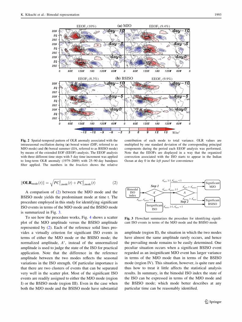
4.1 The bimodal ISO index: the MJO mode
and the BSISO mode
Two distinct typical ISO modes, predominant during boreal
winter (referred to as the MJO mode in honor of the dis-
coverers) and during boreal summer (referred to as the
BSISO mode), are defined. To better describe the state of
the ISO, we took an analogous setting for the EEOF
analysis as Lau and Chan (1985, 1986); The EEOF analysis
with -10 and -5 day lags was applied to the intraseasonal
time-filtered OLR data in the entire tropics between 30�S
and 30�N. The time lag was chosen in this way because of
consideration of its application to real time monitoring. To
derive the MJO (BSISO) mode the data period from
December to February (June–August) was selected.
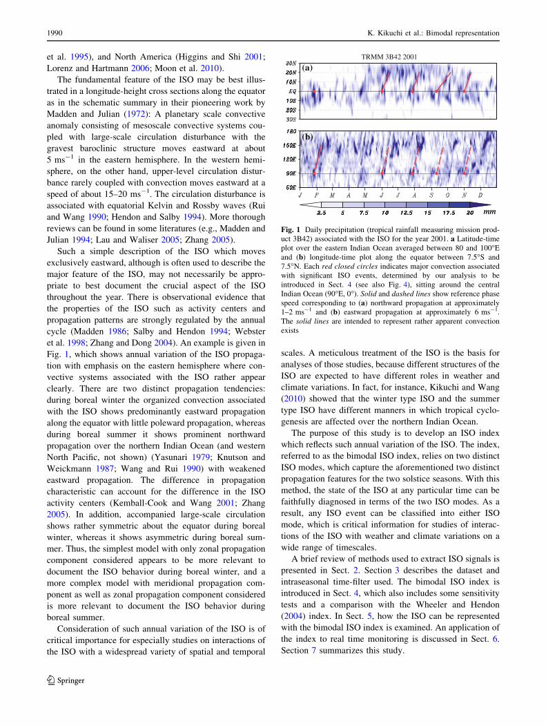
As expected from the previous studies, a pair of the first
two EEOFs represents a half cycle of the ISO for both
modes (Fig. 2). The MJO mode shows a predominant
eastward propagation along the equator that is in accor-
dance with the classical view of the MJO (Madden and
Julian 1972). The BSISO mode shows a prominent north-
ward propagation over the northern Indian Ocean with
weaker eastward propagation along the equator, which
eventually makes an elongated convective band tilting
from northwest to southeast covering a wide range from the
Arabian Sea to the western Pacific. Another prominent
northwestward propagation is seen over the western North
Pacific. These rather complicated features of the BSISO
mode are in good agreement with a recent composite study
using TRMM satellite precipitation data (Wang et al.
2006). Evidently, the lifecycle of the MJO mode and the
BSISO mode have distinctive characteristics.
The bimodal ISO index is based on these two ISO
modes. The EEOF coefficients (principal components, PCs
hereafter) of the MJO mode and the BSISO mode at any
given time can be obtained by projecting the intraseasonal
time-filtered OLR fields onto each mode. The strength and
the phase of the MJO mode and the BSISO mode can be
described by a combination of the first two PCs for each
mode. This is the fundamental step for constructing the
bimodal ISO index.
How to utilize the bimodal ISO index, however, might
depend on analysis. In the following, we provide an
example, which would be one of the most straightforward
ways. For most practical applications, one may want to
identify significant ISO events (Step 1). For that purpose, it
is usual to use the normalized amplitude (A�mode ¼ffiffiffiffiffiffiffiffiffiffiffiffiffiffiffiffiffiffiffiffiffiffiffiffiffiffiffiffiffiffiffiffiffiffiffiffiffiffiffi
PC�21;mode þ PC�22;mode
q
), where PC� is the normalized PC
by one standard deviation during the period the EEOF
analysis was performed and the subscript ‘mode’ represents
either the MJO mode or BSISO mode. A criterion that
A�mode� 1 is regarded as a significant event is perhaps
the most popular (e.g., Wheeler and Hendon 2004). As a
result, significant ISO events can be identified in terms of
the following ISO modes: (1) the MJO mode, (2) the
BSISO mode, and (3) both the MJO mode and the BSISO
mode.
Although, the information listed in step 1 is useful for
certain analyses, in many cases it is more practical to
further determine the predominant mode, i.e. which mode
dominates the ISO event (Step 2). This can be accom-
plished by assuming that the predominant ISO mode at a
given time accounts for a larger amount of the total vari-
ance. The reconstructed OLR anomalies by each mode at
time t are given by
OLRmodeðtÞ ¼ EEOF1;mode � PC1;modeðtÞ þ EEOF2;mode
� PC2;modeðtÞ ð1Þ
where OLRðtÞ includes spatial patterns at -10 and -5 days
as well as 0 day. With the aid of the orthogonality of the
EEOF, the norm (variance) of the reconstructed pattern of
each mode is given by
1992 K. Kikuchi et al.: Bimodal representation
123
OLRmodeðtÞk k ¼ffiffiffiffiffiffiffiffiffiffiffiffiffiffiffiffiffiffiffiffiffiffiffiffiffiffiffiffiffiffiffiffiffiffiffiffiffiffiffiffiffiffiffiffiffiffiffiffiffiffi
PC21;modeðtÞ þ PC2
2;modeðtÞq
ð2Þ
A comparison of (2) between the MJO mode and the
BSISO mode yields the predominant mode at time t. The
procedure employed in this study for identifying significant
ISO events in terms of the MJO mode and the BSISO mode
is summarized in Fig. 3.
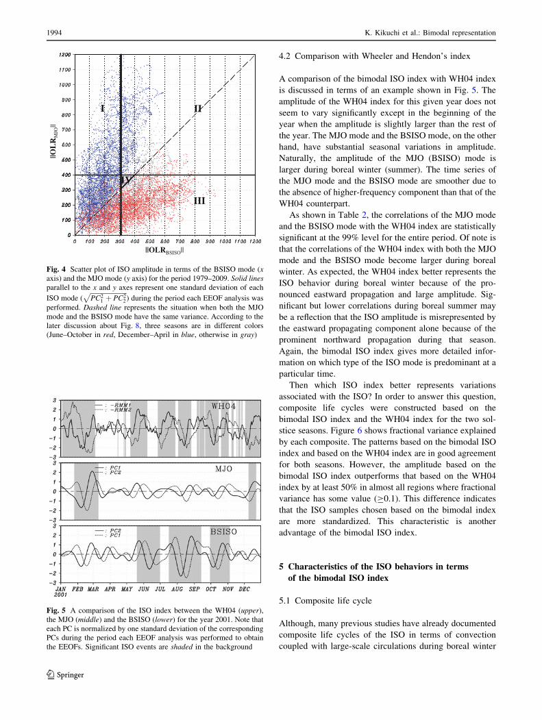
To see how the procedure works, Fig. 4 shows a scatter
plot of the MJO amplitude versus the BSISO amplitude
represented by (2). Each of the reference solid lines pro-
vides a virtually criterion for significant ISO events in
terms of either the MJO mode or the BSISO mode; the
normalized amplitude, A�, instead of the unnormalized
amplitude is used to judge the state of the ISO for practical
application. Note that the difference in the reference
amplitude between the two modes reflects the seasonal
variations in the ISO strength. Of particular importance is
that there are two clusters of events that can be separated
very well in the scatter plot. Most of the significant ISO
events are readily assigned to either the MJO mode (region
I) or the BSISO mode (region III). Even in the case when
both the MJO mode and the BSISO mode have substantial
amplitude (region II), the situation in which the two modes
have almost the same amplitude rarely occurs, and hence
the prevailing mode remains to be easily determined. One
peculiar situation occurs when a significant BSISO event
regarded as an insignificant MJO event has larger variance
in terms of the MJO mode than in terms of the BSISO
mode (region IV). This situation, however, is quite rare and
thus how to treat it little affects the statistical analysis
results. In summary, in the bimodal ISO index the state of
the ISO can be expressed in terms of the MJO mode and
the BSISO mode; which mode better describes at any
particular time can be reasonably identified.
(a) MJOEEOF1 FOEE)%01( 2 (9.4%)
BSISO(b)EEOF2 (8.3%) EEOF1 (9.9%)
W/m2
Fig. 2 Spatial-temporal pattern of OLR anomaly associated with the
intraseasonal oscillation during (a) boreal winter (DJF, referred to as
MJO mode) and (b) boreal summer (JJA, referred to as BSISO mode)
by means of the extended EOF (EEOF) analysis. The EEOF analysis
with three different time steps with 5 day time increment was applied
to long-term OLR anomaly (1979–2009) with 25–90 day bandpass
filter applied. The numbers in the brackets shows the relative
contribution of each mode to total variance. OLR values are
multiplied by one standard deviation of the corresponding principal
components during the period each EEOF analysis was performed.
Note that the EEOFs are displayed in a way that the organized
convection associated with the ISO starts to appear in the Indian
Ocean at day 0 in the left panel for convenience
1,1 ** <≥ AASignificant
BSISOMJO
**Step 1Bimodal
MJO1, ** ≥BSISOMJO AA
BSISOMJO AA >
*ISOindex
**
A A
Significant MJOBSISO AA >1, ** <BSISOMJO AAStep 2
BSISO1,1 ** <≥ MJOBSISO AAInsignificant
ISO
Fig. 3 Flowchart summarizes the procedure for identifying signifi-
cant ISO events in terms of the MJO mode and the BSISO mode
K. Kikuchi et al.: Bimodal representation 1993
123
4.2 Comparison with Wheeler and Hendon’s index
A comparison of the bimodal ISO index with WH04 index
is discussed in terms of an example shown in Fig. 5. The
amplitude of the WH04 index for this given year does not
seem to vary significantly except in the beginning of the
year when the amplitude is slightly larger than the rest of
the year. The MJO mode and the BSISO mode, on the other
hand, have substantial seasonal variations in amplitude.
Naturally, the amplitude of the MJO (BSISO) mode is
larger during boreal winter (summer). The time series of
the MJO mode and the BSISO mode are smoother due to
the absence of higher-frequency component than that of the
WH04 counterpart.
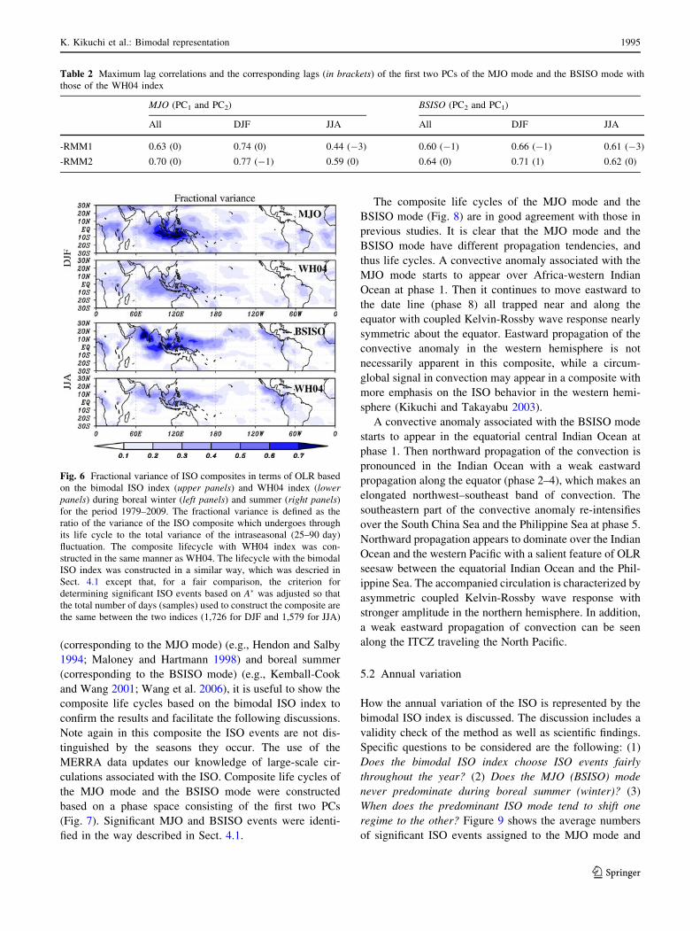
As shown in Table 2, the correlations of the MJO mode
and the BSISO mode with the WH04 index are statistically
significant at the 99% level for the entire period. Of note is
that the correlations of the WH04 index with both the MJO
mode and the BSISO mode become larger during boreal
winter. As expected, the WH04 index better represents the
ISO behavior during boreal winter because of the pro-
nounced eastward propagation and large amplitude. Sig-
nificant but lower correlations during boreal summer may
be a reflection that the ISO amplitude is misrepresented by
the eastward propagating component alone because of the
prominent northward propagation during that season.
Again, the bimodal ISO index gives more detailed infor-
mation on which type of the ISO mode is predominant at a
particular time.
Then which ISO index better represents variations
associated with the ISO? In order to answer this question,
composite life cycles were constructed based on the
bimodal ISO index and the WH04 index for the two sol-
stice seasons. Figure 6 shows fractional variance explained
by each composite. The patterns based on the bimodal ISO
index and based on the WH04 index are in good agreement
for both seasons. However, the amplitude based on the
bimodal ISO index outperforms that based on the WH04
index by at least 50% in almost all regions where fractional
variance has some value (C0.1). This difference indicates
that the ISO samples chosen based on the bimodal index
are more standardized. This characteristic is another
advantage of the bimodal ISO index.
5 Characteristics of the ISO behaviors in terms
of the bimodal ISO index
5.1 Composite life cycle
Although, many previous studies have already documented
composite life cycles of the ISO in terms of convection
coupled with large-scale circulations during boreal winter
I III II
MJO
||L
R||O
IVIV
III
||OLRBSISO||
Fig. 4 Scatter plot of ISO amplitude in terms of the BSISO mode (xaxis) and the MJO mode (y axis) for the period 1979–2009. Solid linesparallel to the x and y axes represent one standard deviation of each
ISO mode (ffiffiffiffiffiffiffiffiffiffiffiffiffiffiffiffiffiffiffiffiffiffiffi
PC21 þ PC2
2
p
) during the period each EEOF analysis was
performed. Dashed line represents the situation when both the MJO
mode and the BSISO mode have the same variance. According to the
later discussion about Fig. 8, three seasons are in different colors
(June–October in red, December–April in blue, otherwise in gray)
Fig. 5 A comparison of the ISO index between the WH04 (upper),
the MJO (middle) and the BSISO (lower) for the year 2001. Note that
each PC is normalized by one standard deviation of the corresponding
PCs during the period each EEOF analysis was performed to obtain
the EEOFs. Significant ISO events are shaded in the background
1994 K. Kikuchi et al.: Bimodal representation
123
(corresponding to the MJO mode) (e.g., Hendon and Salby
1994; Maloney and Hartmann 1998) and boreal summer
(corresponding to the BSISO mode) (e.g., Kemball-Cook
and Wang 2001; Wang et al. 2006), it is useful to show the
composite life cycles based on the bimodal ISO index to
confirm the results and facilitate the following discussions.
Note again in this composite the ISO events are not dis-
tinguished by the seasons they occur. The use of the
MERRA data updates our knowledge of large-scale cir-
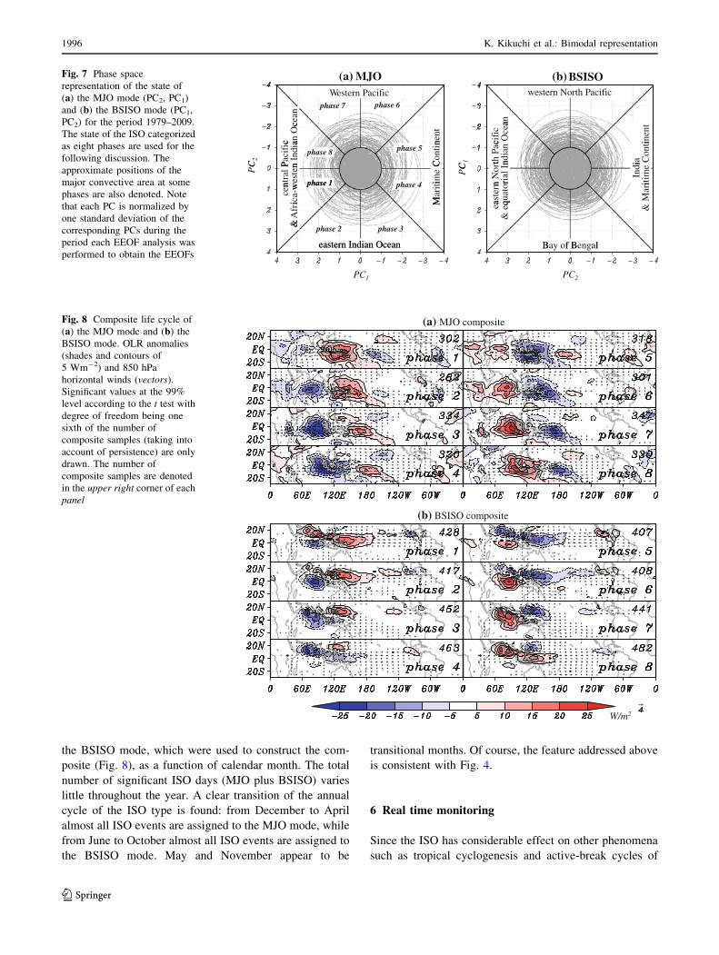
culations associated with the ISO. Composite life cycles of
the MJO mode and the BSISO mode were constructed
based on a phase space consisting of the first two PCs
(Fig. 7). Significant MJO and BSISO events were identi-
fied in the way described in Sect. 4.1.
The composite life cycles of the MJO mode and the
BSISO mode (Fig. 8) are in good agreement with those in
previous studies. It is clear that the MJO mode and the
BSISO mode have different propagation tendencies, and
thus life cycles. A convective anomaly associated with the
MJO mode starts to appear over Africa-western Indian
Ocean at phase 1. Then it continues to move eastward to
the date line (phase 8) all trapped near and along the
equator with coupled Kelvin-Rossby wave response nearly
symmetric about the equator. Eastward propagation of the
convective anomaly in the western hemisphere is not
necessarily apparent in this composite, while a circum-
global signal in convection may appear in a composite with
more emphasis on the ISO behavior in the western hemi-
sphere (Kikuchi and Takayabu 2003).
A convective anomaly associated with the BSISO mode
starts to appear in the equatorial central Indian Ocean at
phase 1. Then northward propagation of the convection is
pronounced in the Indian Ocean with a weak eastward
propagation along the equator (phase 2–4), which makes an
elongated northwest–southeast band of convection. The
southeastern part of the convective anomaly re-intensifies
over the South China Sea and the Philippine Sea at phase 5.
Northward propagation appears to dominate over the Indian
Ocean and the western Pacific with a salient feature of OLR
seesaw between the equatorial Indian Ocean and the Phil-
ippine Sea. The accompanied circulation is characterized by
asymmetric coupled Kelvin-Rossby wave response with
stronger amplitude in the northern hemisphere. In addition,
a weak eastward propagation of convection can be seen
along the ITCZ traveling the North Pacific.
5.2 Annual variation
How the annual variation of the ISO is represented by the
bimodal ISO index is discussed. The discussion includes a
validity check of the method as well as scientific findings.
Specific questions to be considered are the following: (1)
Does the bimodal ISO index choose ISO events fairly
throughout the year? (2) Does the MJO (BSISO) mode
never predominate during boreal summer (winter)? (3)
When does the predominant ISO mode tend to shift one
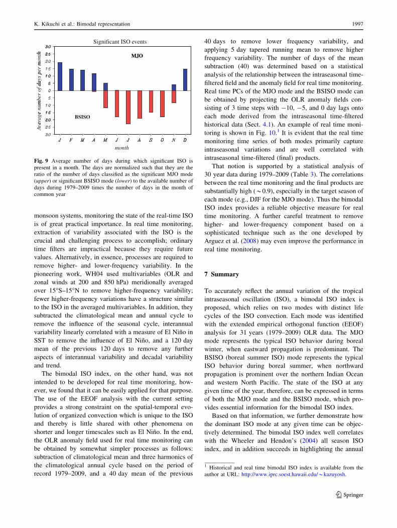
regime to the other? Figure 9 shows the average numbers
of significant ISO events assigned to the MJO mode and
Table 2 Maximum lag correlations and the corresponding lags (in brackets) of the first two PCs of the MJO mode and the BSISO mode with
those of the WH04 index
MJO (PC1 and PC2) BSISO (PC2 and PC1)
All DJF JJA All DJF JJA
-RMM1 0.63 (0) 0.74 (0) 0.44 (-3) 0.60 (-1) 0.66 (-1) 0.61 (-3)
-RMM2 0.70 (0) 0.77 (-1) 0.59 (0) 0.64 (0) 0.71 (1) 0.62 (0)
Fig. 6 Fractional variance of ISO composites in terms of OLR based
on the bimodal ISO index (upper panels) and WH04 index (lowerpanels) during boreal winter (left panels) and summer (right panels)
for the period 1979–2009. The fractional variance is defined as the
ratio of the variance of the ISO composite which undergoes through
its life cycle to the total variance of the intraseasonal (25–90 day)
fluctuation. The composite lifecycle with WH04 index was con-
structed in the same manner as WH04. The lifecycle with the bimodal
ISO index was constructed in a similar way, which was descried in
Sect. 4.1 except that, for a fair comparison, the criterion for
determining significant ISO events based on A� was adjusted so that
the total number of days (samples) used to construct the composite are
the same between the two indices (1,726 for DJF and 1,579 for JJA)
K. Kikuchi et al.: Bimodal representation 1995
123
the BSISO mode, which were used to construct the com-
posite (Fig. 8), as a function of calendar month. The total
number of significant ISO days (MJO plus BSISO) varies
little throughout the year. A clear transition of the annual
cycle of the ISO type is found: from December to April
almost all ISO events are assigned to the MJO mode, while
from June to October almost all ISO events are assigned to
the BSISO mode. May and November appear to be
transitional months. Of course, the feature addressed above
is consistent with Fig. 4.
6 Real time monitoring
Since the ISO has considerable effect on other phenomena
such as tropical cyclogenesis and active-break cycles of
(a) MJO BSISOWestern Pacific western North Pacific
phase 6phase 7
cean
a n
c an O
c
nent
cifi
cO
cea
inen
t
C2
phase 8
P aci
fic
n In
dia
Con
tin
th P
acnd
ian
ia Con
tiphase 5
C1
PC
phase 1ntra
l Pw
este
n
ime
C
n N
ort
rial
In
Ind i
itim
e
PC
phase 1
cen
ica-
w
Mar
itiphase 4
aste
r nqu
ator
Mar
i
& A
fri M e a
& e
q
&
phase 2 phase 3
eastern Indian Ocean
&
B f B leastern Indian Ocean Bay of Bengal
PC1 PC2
(b)Fig. 7 Phase space
representation of the state of
(a) the MJO mode (PC2, PC1)
and (b) the BSISO mode (PC1,
PC2) for the period 1979–2009.
The state of the ISO categorized
as eight phases are used for the
following discussion. The
approximate positions of the
major convective area at some
phases are also denoted. Note
that each PC is normalized by
one standard deviation of the
corresponding PCs during the
period each EEOF analysis was
performed to obtain the EEOFs
(a) MJO composite
(b) BSISO composite
W/m2
Fig. 8 Composite life cycle of
(a) the MJO mode and (b) the
BSISO mode. OLR anomalies
(shades and contours of
5 Wm-2) and 850 hPa
horizontal winds (vectors).
Significant values at the 99%
level according to the t test with
degree of freedom being one
sixth of the number of
composite samples (taking into
account of persistence) are only
drawn. The number of
composite samples are denoted
in the upper right corner of each
panel
1996 K. Kikuchi et al.: Bimodal representation
123
monsoon systems, monitoring the state of the real-time ISO
is of great practical importance. In real time monitoring,
extraction of variability associated with the ISO is the
crucial and challenging process to accomplish; ordinary
time filters are impractical because they require future
values. Alternatively, in essence, processes are required to
remove higher- and lower-frequency variability. In the
pioneering work, WH04 used multivariables (OLR and
zonal winds at 200 and 850 hPa) meridionally averaged
over 15�S–15�N to remove higher-frequency variability;
fewer higher-frequency variations have a structure similar
to the ISO in the averaged multivariables. In addition, they
subtracted the climatological mean and annual cycle to
remove the influence of the seasonal cycle, interannual
variability linearly correlated with a measure of El Nino in
SST to remove the influence of El Nino, and a 120 day
mean of the previous 120 days to remove any further
aspects of interannual variability and decadal variability
and trend.
The bimodal ISO index, on the other hand, was not
intended to be developed for real time monitoring, how-
ever, we found that it can be easily applied for that purpose.
The use of the EEOF analysis with the current setting
provides a strong constraint on the spatial-temporal evo-
lution of organized convection which is unique to the ISO
and thereby is little shared with other phenomena on
shorter and longer timescales such as El Nino. In the end,
the OLR anomaly field used for real time monitoring can
be obtained by somewhat simpler processes as follows:
subtraction of climatological mean and three harmonics of
the climatological annual cycle based on the period of
record 1979–2009, and a 40 day mean of the previous
40 days to remove lower frequency variability, and
applying 5 day tapered running mean to remove higher
frequency variability. The number of days of the mean
subtraction (40) was determined based on a statistical
analysis of the relationship between the intraseasonal time-
filtered field and the anomaly field for real time monitoring.
Real time PCs of the MJO mode and the BSISO mode can
be obtained by projecting the OLR anomaly fields con-
sisting of 3 time steps with -10, -5, and 0 day lags onto
each mode derived from the intraseasonal time-filtered
historical data (Sect. 4.1). An example of real time moni-
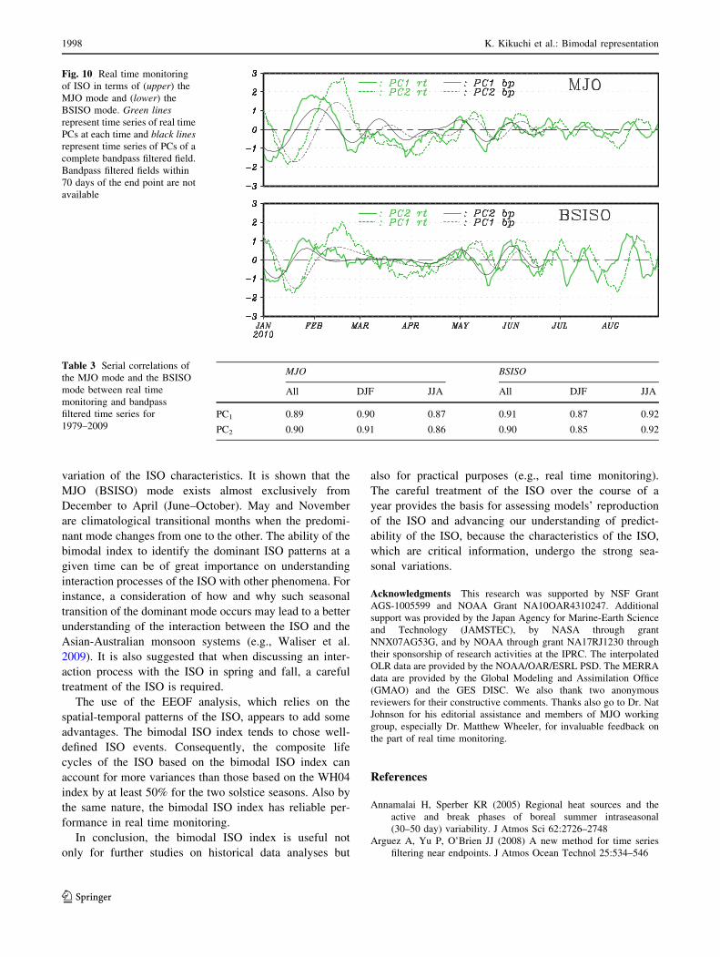
toring is shown in Fig. 10.1 It is evident that the real time
monitoring time series of both modes primarily capture
intraseasonal variations and are well correlated with
intraseasonal time-filtered (final) products.
That notion is supported by a statistical analysis of
30 year data during 1979–2009 (Table 3). The correlations
between the real time monitoring and the final products are
substantially high (*0.9), especially in the target season of
each mode (e.g., DJF for the MJO mode). Thus the bimodal
ISO index provides a reliable objective measure for real
time monitoring. A further careful treatment to remove
higher- and lower-frequency component based on a
sophisticated technique such as the one developed by
Arguez et al. (2008) may even improve the performance in
real time monitoring.
7 Summary
To accurately reflect the annual variation of the tropical
intraseasonal oscillation (ISO), a bimodal ISO index is
proposed, which relies on two modes with distinct life
cycles of the ISO convection. Each mode was identified
with the extended empirical orthogonal function (EEOF)
analysis for 31 years (1979–2009) OLR data. The MJO
mode represents the typical ISO behavior during boreal
winter, when eastward propagation is predominant. The
BSISO (boreal summer ISO) mode represents the typical
ISO behavior during boreal summer, when northward
propagation is prominent over the northern Indian Ocean
and western North Pacific. The state of the ISO at any
given time of the year, therefore, can be expressed in terms
of both the MJO mode and the BSISO mode, which pro-
vides essential information for the bimodal ISO index.
Based on that information, we further demonstrate how
the dominant ISO mode at any given time can be objec-
tively determined. The bimodal ISO index well correlates
with the Wheeler and Hendon’s (2004) all season ISO
index, and in addition succeeds in highlighting the annual
Significant ISO eventsh
MJO
mon
th MJO
per
mda
ys p
of d
am
ber
e nu
mer
age
BSISO
Ave
month
Fig. 9 Average number of days during which significant ISO is
present in a month. The days are normalized such that they are the
ratio of the number of days classified as the significant MJO mode
(upper) or significant BSISO mode (lower) to the available number of
days during 1979–2009 times the number of days in the month of
common year
1 Historical and real time bimodal ISO index is available from the
author at URL: http://www.iprc.soest.hawaii.edu/*kazuyosh.
K. Kikuchi et al.: Bimodal representation 1997
123
variation of the ISO characteristics. It is shown that the
MJO (BSISO) mode exists almost exclusively from
December to April (June–October). May and November
are climatological transitional months when the predomi-
nant mode changes from one to the other. The ability of the
bimodal index to identify the dominant ISO patterns at a
given time can be of great importance on understanding
interaction processes of the ISO with other phenomena. For
instance, a consideration of how and why such seasonal
transition of the dominant mode occurs may lead to a better
understanding of the interaction between the ISO and the
Asian-Australian monsoon systems (e.g., Waliser et al.
2009). It is also suggested that when discussing an inter-
action process with the ISO in spring and fall, a careful
treatment of the ISO is required.
The use of the EEOF analysis, which relies on the
spatial-temporal patterns of the ISO, appears to add some
advantages. The bimodal ISO index tends to chose well-
defined ISO events. Consequently, the composite life
cycles of the ISO based on the bimodal ISO index can
account for more variances than those based on the WH04
index by at least 50% for the two solstice seasons. Also by
the same nature, the bimodal ISO index has reliable per-
formance in real time monitoring.
In conclusion, the bimodal ISO index is useful not
only for further studies on historical data analyses but
also for practical purposes (e.g., real time monitoring).
The careful treatment of the ISO over the course of a
year provides the basis for assessing models’ reproduction
of the ISO and advancing our understanding of predict-
ability of the ISO, because the characteristics of the ISO,
which are critical information, undergo the strong sea-
sonal variations.
Acknowledgments This research was supported by NSF Grant
AGS-1005599 and NOAA Grant NA10OAR4310247. Additional
support was provided by the Japan Agency for Marine-Earth Science
and Technology (JAMSTEC), by NASA through grant
NNX07AG53G, and by NOAA through grant NA17RJ1230 through
their sponsorship of research activities at the IPRC. The interpolated
OLR data are provided by the NOAA/OAR/ESRL PSD. The MERRA
data are provided by the Global Modeling and Assimilation Office
(GMAO) and the GES DISC. We also thank two anonymous
reviewers for their constructive comments. Thanks also go to Dr. Nat
Johnson for his editorial assistance and members of MJO working
group, especially Dr. Matthew Wheeler, for invaluable feedback on
the part of real time monitoring.
References
Annamalai H, Sperber KR (2005) Regional heat sources and the
active and break phases of boreal summer intraseasonal
(30–50 day) variability. J Atmos Sci 62:2726–2748
Arguez A, Yu P, O’Brien JJ (2008) A new method for time series
filtering near endpoints. J Atmos Ocean Technol 25:534–546
Fig. 10 Real time monitoring
of ISO in terms of (upper) the
MJO mode and (lower) the
BSISO mode. Green linesrepresent time series of real time
PCs at each time and black linesrepresent time series of PCs of a
complete bandpass filtered field.
Bandpass filtered fields within
70 days of the end point are not
available
Table 3 Serial correlations of
the MJO mode and the BSISO
mode between real time
monitoring and bandpass
filtered time series for
1979–2009
MJO BSISO
All DJF JJA All DJF JJA
PC1 0.89 0.90 0.87 0.91 0.87 0.92
PC2 0.90 0.91 0.86 0.90 0.85 0.92
1998 K. Kikuchi et al.: Bimodal representation
123
Bosilovich MG, Schubert SD, Rienecker M, Todling R, Suarez M,
Bacmeister J, Gelaro R, Kim G-K, Stajner I, Chen J (2006)
NASA’s modern era retrospective-analysis for research and
applications. US CLIVAR Var 4:5–8
Chen SS, Houze RA Jr (1997) Diurnal variation and life-cycle of deep
convective systems over the tropical pacific warm pool. Quart J
Roy Met Soc 123:357–388
Duchon CE (1979) Lanczos filtering in one and two dimensions.
J Appl Meteorol 18:1016–1022
Hendon HH, Liebmann B (1990) A composite study of onset of the
Australian summer monsoon. J Atmos Sci 47:2227–2240
Hendon HH, Salby ML (1994) The life cycle of the Madden-Julian
oscillation. J Atmos Sci 51:2225–2237
Higgins RW, Shi W (2001) Intercomparison of the principal modes of
interannual and intraseasonal variability of the North American
monsoon system. J Clim 14:403–417
Hsu HH (1996) Global view of the intraseasonal oscillation during
northern winter. J Clim 9:2386–2406
Ichikawa H, Yasunari T (2008) Intraseasonal variability in diurnal
rainfall over New Guinea and the surrounding oceans during
austral summer. J Clim 21:2852–2868
Jones C, Carvalho LMV, Higgins RW, Waliser DE, Schemm JKE
(2004) Climatology of tropical intraseasonal convective anom-
alies: 1979–2002. J Clim 17:523–539
Julian PR, Madden R (1981) Comments on a paper by T. Yasunari, a
quasi-stationary appearance of 30–40-day period in the cloud-
iness fluctuations during the summer monsoon over India.
J Meteor Soc Jpn 59:435–437
Kajikawa Y, Yasunari T (2005) Interannual variability of the 10–25-
and 30–60-day variation over the South China Sea during boreal
summer. Geophys Res Lett 32:L04710. doi: 10.1029/2004
GL021836
Kayano MT, Kousky VE (1999) Intraseasonal (30–60 day) variability
in the global tropics: principal modes and their evolution. Tellus
51:373–386
Kemball-Cook S, Wang B (2001) Equatorial waves and air-sea
interaction in the boreal summer intraseasonal oscillation. J Clim
14:2923–2942
Kessler WS, McPhaden MJ, Weickmann KM (1995) Forcing of
intraseasonal Kelvin waves in the equatorial Pacific. J Geophys
Res 100:10613–10631
Kikuchi K, Takayabu YN (2003) Equatorial circumnavigation of
moisture signal associated with the Madden-Julian oscillation
(MJO) during boreal winter. J Meteor Soc Jpn 81:851–869
Kikuchi K, Wang B (2010) Formation of tropical cyclones in the
northern Indian Ocean associated with two types of tropical
intraseasonal oscillation modes. J Meteor Soc Jpn 88:475–496
Knutson TR, Weickmann KM (1987) 30–60 day atmospheric oscil-
lations: composite life-cycles of convection and circulation
anomalies. Mon Wea Rev 115:1407–1436
Lau KM, Chan PH (1985) Aspects of the 40–50 day oscillation during
the northern winter as inferred from outgoing long wave
radiation. Mon Wea Rev 113:1889–1909
Lau KM, Chan PH (1986) Aspects of the 40–50 day oscillation during
the northern summer as inferred from outgoing long wave
radiation. Mon Wea Rev 114:1354–1367
Lau KM, Chan PH (1988) Intraseasonal and interannual variations of
tropical convection: a possible link between the 40–50 day
oscillation and ENSO? J Atmos Sci 45:506–521
Lau KMW, Waliser DE (eds) (2005) Intraseasonal variability in the
atmosphere-ocean climate system. Springer, Berlin, p 436
Liebmann B, Smith CA (1996) Description of a complete (interpo-
lated) outgoing longwave radiation dataset. Bull Am Meteor Soc
77:1275–1277
Lorenz DJ, Hartmann DL (2006) The effect of the MJO on the North
American monsoon. J Clim 19:333–343
Madden RA (1986) Seasonal-variations of the 40–50 day oscillation
in the tropics. J Atmos Sci 43:3138–3158
Madden RA, Julian PR (1971) Detection of a 40–50 day oscillation in
the zonal wind in the tropical Pacific. J Atmos Sci 28:702–708
Madden RA, Julian PR (1972) Description of global-scale circulation
cells in tropics with a 40–50 day period. J Atmos Sci
29:1109–1123
Madden RA, Julian PR (1994) Observations of the 40–50-day tropical
oscillation: a review. Mon Wea Rev 122:814–837
Maloney ED, Hartmann DL (1998) Frictional moisture convergence
in a composite life cycle of the Madden-Julian oscillation. J Clim
11:2387–2403
Maloney ED, Hartmann DL (2000a) Modulation of eastern north
Pacific hurricanes by the Madden-Julian oscillation. J Clim
13:1451–1460
Maloney ED, Hartmann DL (2000b) Modulation of hurricane activity
in the Gulf of Mexico by the Madden-Julian oscillation. Science
287:2002–2004
McBride JL, Davidson NE, Puri K, Tyrell GC (1995) The flow during
TOGA COARE as diagnosed by the BMRC tropical analysis and
prediction system. Mon Wea Rev 123:717–736
Miller AJ, Zhou S, Yang SK (2003) Relationship of the Arctic and
Antarctic oscillations to the outgoing longwave radiation. J Clim
16:1583–1592
Molinari J, Vollaro D (2000) Planetary- and synoptic-scale influences
on eastern Pacific tropical cyclogenesis. Mon Wea Rev
128:3296–3307
Moon J-Y, Wang B, Ha K-J (2010) ENSO regulation of MJO
teleconnection. Clim Dyn, (in press)
Rui H, Wang B (1990) Development characteristics and dynamic
structure of tropical intraseasonal convection anomalies. J Atmos
Sci 47:357–379
Salby ML, Hendon HH (1994) Intraseasonal behavior of clouds,
temperature, and motion in the tropics. J Atmos Sci 51:2207–2224
Slingo JM, Rowell DP, Sperber KR, Nortley E (1999) On the
predictability of the interannual behaviour of the Madden-Julian
oscillation and its relationship with El Nino. Quart J Roy Met
Soc 125:583–609
Takayabu YN, Iguchi T, Kachi M, Shibata A, Kanzawa H (1999)
Abrupt termination of the 1997–1998 El Nino in response to a
Madden-Julian oscillation. Nature 402:279–282
von Storch H, Xu J (1990) Principal oscillation pattern analysis of the
30–60-day oscillation in the tropical troposphere. Clim Dyn
4:175–190
Waliser DE, Murtugudde R, Lucas LE (2003a) Indo-Pacific Ocean
response to atmospheric intraseasonal variability: 1. Austral
summer and the Madden-Julian oscillation. J Geophys Res
108(C5):3160. doi: 10.1029/2002JC001620
Waliser DE, Lau KM, Stern W, Jones C (2003b) Potential predict-
ability of the Madden-Julian oscillation. Bull Am Meteor Soc
84:33–50
Waliser DE, Murtugudde R, Lucas LE (2004) Indo-Pacific Ocean
response to atmospheric intraseasonal variability: 2. Boreal
summer and the intraseasonal oscillation. J Geophys Res
109:C03030. doi: 10.1029/2003JC002002
Waliser D, Sperber K, Hendon H, Kim D, Wheeler M, Weickmann K,
Zhang C, Donner L, Gottschalck J, Higgins W, Kang IS, Legler
D, Moncrieff M, Vitart F, Wang B, Wang W, Woolnough S,
Maloney E, Schubert S, Stern W (2009) MJO simulation
diagnostics. J Clim 22:3006–3030
Wang B, Rui H (1990) Synoptic climatology of transient tropical
intraseasonal convection anomalies: 1975–1985. Meteor Atmos
Phys 44:43–61
Wang B, Webster P, Kikuchi K, Yasunari T, Qi YJ (2006) Boreal
summer quasi-monthly oscillation in the global tropics. Clim
Dyn 27:661–675
K. Kikuchi et al.: Bimodal representation 1999
123

Weare BC, Nasstrom JS (1982) Examples of extended empirical
orthogonal function analyses. Mon Wea Rev 110:481–485
Webster PJ, Magana VO, Palmer TN, Shukla J, Tomas RA, Yanai M,
Yasunari T (1998) Monsoons: processes, predictability, and the
prospects for prediction. J Geophys Res 103:14451–14510
Wheeler MC, Hendon HH (2004) An all-season real-time multivariate
MJO index: development of an index for monitoring and
prediction. Mon Wea Rev 132:1917–1932
Yasunari T (1979) Cloudiness fluctuations associated with the
northern hemisphere summer monsoon. J Meteor Soc Jpn
57:227–242
Zhang CD (2005) Madden-Julian oscillation. Rev Geophys
43:RG2003. doi:10.1029/2004RG000158
Zhang CD, Dong M (2004) Seasonality in the Madden-Julian
oscillation. J Clim 17:3169–3180
Zhang CD, Hendon HH (1997) Propagating and standing components
of the intraseasonal oscillation in tropical convection. J Atmos
Sci 54:741–752
2000 K. Kikuchi et al.: Bimodal representation
123