relationship between exploitation, oscillation, msy and extinction
TRANSCRIPT

Seediscussions,stats,andauthorprofilesforthispublicationat:https://www.researchgate.net/publication/264127848
Relationshipbetweenexploitation,oscillation,MSYandextinction
ARTICLEinMATHEMATICALBIOSCIENCES·JULY2014
ImpactFactor:1.3·DOI:10.1016/j.mbs.2014.07.005·Source:PubMed
READS
74
3AUTHORS,INCLUDING:
GhoshBapan
IndianInstituteofEngineeringScienceand…
15PUBLICATIONS76CITATIONS
SEEPROFILE
Allin-textreferencesunderlinedinbluearelinkedtopublicationsonResearchGate,
lettingyouaccessandreadthemimmediately.
Availablefrom:GhoshBapan
Retrievedon:09February2016
Mathematical Biosciences 256 (2014) 1–9
Contents lists available at ScienceDirect
Mathematical Biosciences
journal homepage: www.elsevier .com/locate /mbs
Relationship between exploitation, oscillation, MSY and extinction
http://dx.doi.org/10.1016/j.mbs.2014.07.0050025-5564/� 2014 Elsevier Inc. All rights reserved.
⇑ Corresponding author. Current Address: Inria, Centre de Recherche Inria SophiaAntipolis, Mediterranee, BIOCORE Team, 06902 Sophia Antipolis, France. Tel.: +9133 26684561; fax: +91 33 26682916.
E-mail addresses: [email protected] (B. Ghosh), [email protected](T.K. Kar), [email protected] (T. Legovic).
Bapan Ghosh a,⇑, T.K. Kar a, T. Legovic b
a Department of Mathematics, Indian Institute of Engineering Science and Technology, Shibpur (Formerly Bengal Engineering and Science University, Shibpur), Howrah 711103,West Bengal, Indiab R. Boskovic Institute, POB 180, HR-10 002 Zagreb, Croatia
a r t i c l e i n f o a b s t r a c t
Article history:Received 11 December 2013Received in revised form 8 July 2014Accepted 10 July 2014Available online 19 July 2014
Keywords:Allee effectMaximum sustainable yieldMean stockStable stockOscillationExtinction
We give answers to two important problems arising in current fisheries: (i) how maximum sustainableyield (MSY) policy is influenced by the initial population level, and (ii) how harvesting, oscillation andMSY are related to each other in prey–predator systems. To examine the impact of initial populationon exploitation, we analyze a single species model with strong Allee effect. It is found that even whenthe MSY exists, the dynamic solution may not converge to the equilibrium stock if the initial populationlevel is higher but near the critical threshold level. In a prey–predator system with Allee effect in the preyspecies, the initial population does not have such important impact neither on MSY nor on maximum sus-tainable total yield (MSTY). However, harvesting the top predator may cause extinction of all species ifodd number of trophic levels exist in the ecosystem. With regard to the second problem, we studytwo prey–predator models and establish that increasing harvesting effort either on prey, predator or bothprey and predator destroys previously existing oscillation. Moreover, equilibrium stock both at MSY andMSTY level is stable. We also discuss the validity of found results to other prey–predator systems.
� 2014 Elsevier Inc. All rights reserved.
1. Introduction
Human impact on natural ecosystems, especially by commer-cial fisheries, is diverse and accelerating. Open access fishery,over-exploitation and destructive fishing practices such astrawling are the main reasons for stock depletion. As a result, thenumber of marine species in danger of extinction is increasing.The proposed concept to remedy the situation is the maximumsustainable yield (MSY) policy, which is the maximum proportionthat can be removed from stock over time without causing popula-tion decline below the optimum level. The MSY concept wasformulated by Russell [28], Hjort et al. [13] and Graham [12]. Adecade following World War II was a golden period of the conceptdevelopment (see [7,25,29]; Ricker, [26]). Recently, The Interna-tional Council for the Exploration of the Sea (ICES) reports that81% of the stocks assessed are overfished and that for some stocksfishing mortality is as much as five times higher than that neededto achieve MSY. Similarly, 75 % of fish stocks in european watersare overfished [5].
In this context, the encouragement by the World Summit onSustainable Development (Johannesburg, 2002) to apply MSY pol-icy in ecosystems is really important. Contrary to the above advice,Walters et al. [33] have shown that the widespread application ofMSY policy would, in general, cause severe deterioration in ecosys-tem structure, in particular the loss of top predator species. Matsu-da and Abrams [20] also examine the MSY policy in various foodweb models and report that harvesting of a relatively few speciesat equilibrium causes the extinction of a significant fraction of spe-cies from the food web. Legovic [16] shows that ten out of sixteengroups of demersal fish in the Adriatic Sea have been harvestedbeyond MSY level. Legovic et al. [19] established that harvestingof both prey and predator towards prey MSY level causesextinction of the predator species. In the case of two or more inde-pendent populations each having logistic growth rate with approx-imately equal carrying capacities, Legovic and Gecek [17] concludethat MSTY (maximum sustainable total yield from both species)exists under independent efforts with the coexistence of species,but for equal harvesting effort, the species with lower biotic poten-tial may go to extinction. Smith et al. [30] also conclude that fish-ing at conventional MSY level can have large impacts on otherparts of the ecosystem, particularly, when they constitute a highproportion of the biomass in the ecosystem or are highly connectedin the food web. Recently, Legovic and Gecek [18] concluded thatspecies with lower biotic potential and carrying capacity may be

2 B. Ghosh et al. / Mathematical Biosciences 256 (2014) 1–9
driven to extinction to reach MSTY level under equal harvestingeffort, especially, if these species weakly cooperate with the restof a mutualistic community. They also employed selective harvest-ing efforts on competing species [8] to reach MSTY level andobserve that it does not affect the system stability character,though some populations may be too small to persist in nature.Kar and Ghosh [15] note that prey harvesting at MSY level in aprey–predator system with crowding effect among predator spe-cies may not cause any extinction. In the same work, they alsoassert that in a ratio-dependent prey–predator system, harvestingthe prey species at MSY level does not cause extinction of the pred-ator species. In a generalist prey–predator system, Ghosh and Kar[10] have shown that predator species can persist when prey isharvested at the MSY level. Ghosh and Kar [9] propose that preyharvesting at MSY level always becomes a sustainable fishing pol-icy in a prey–predator system, where prey-dependent carryingcapacity for predator is incorporated. Very recently, Ghosh andKar [11] pointed out that application of nonlinear harvesting func-tion may prevent the extinction of the predator species. Dennis [2]mentioned that a critical density is a lower unstable equilibrium ina single species model with Allee effect. Under constant effortstrategy, both the lower unstable state and the upper stable statemarge together and disappear for some critical effort. Hence, theyield curve has an abrupt discontinuity and population goes toextinction when the effort crosses the critical threshold. In thisregard, he suggested that resource would be close to exterminationwhen harvesting reaches the maximum level. Stephens and Suth-erland [31] have shown that harvesting may cause extinction ina single species model with strong Allee effect. Kar and Matsuda[14] accurately determined the MSY at equilibrium for a single spe-cies model with Allee effect. Considering the present state of fishresources, the effect of initial population level on MSY policyremains unknown. Moreover, most of the above theoretical resultsare based on prey–predator systems with bilinear interaction.Therefore, effect of MSY on corresponding stocks in oscillatory preypredator systems [27,23,24,6] is also unknown.
The paper is organized as follows. In Section 2, we revisit theMSY policy based on single species logistic model. Section 3 exam-ines the existence of MSY in a single species model incorporatingthe Allee effect and compares the results with that of single specieslogistic model. Section 4 is devoted to understanding the influenceof initial population level to achieve MSY and MSTY. In Section 5,we examine whether harvesting of either prey, predator or bothspecies creates or destroys oscillations in prey–predator systems.In addition, we establish that stock at MSY and MSTY level is sta-ble. Finally, in Section 6, the main results are discussed in viewof their applicability to other classes of models.
2. Revisiting traditional MSY
Widely studied single species mathematical model with logisticgrowth function and proportional harvesting [29,3] is given by:
dxdt¼ rx 1� x
K
� �� qex; ð2:1Þ
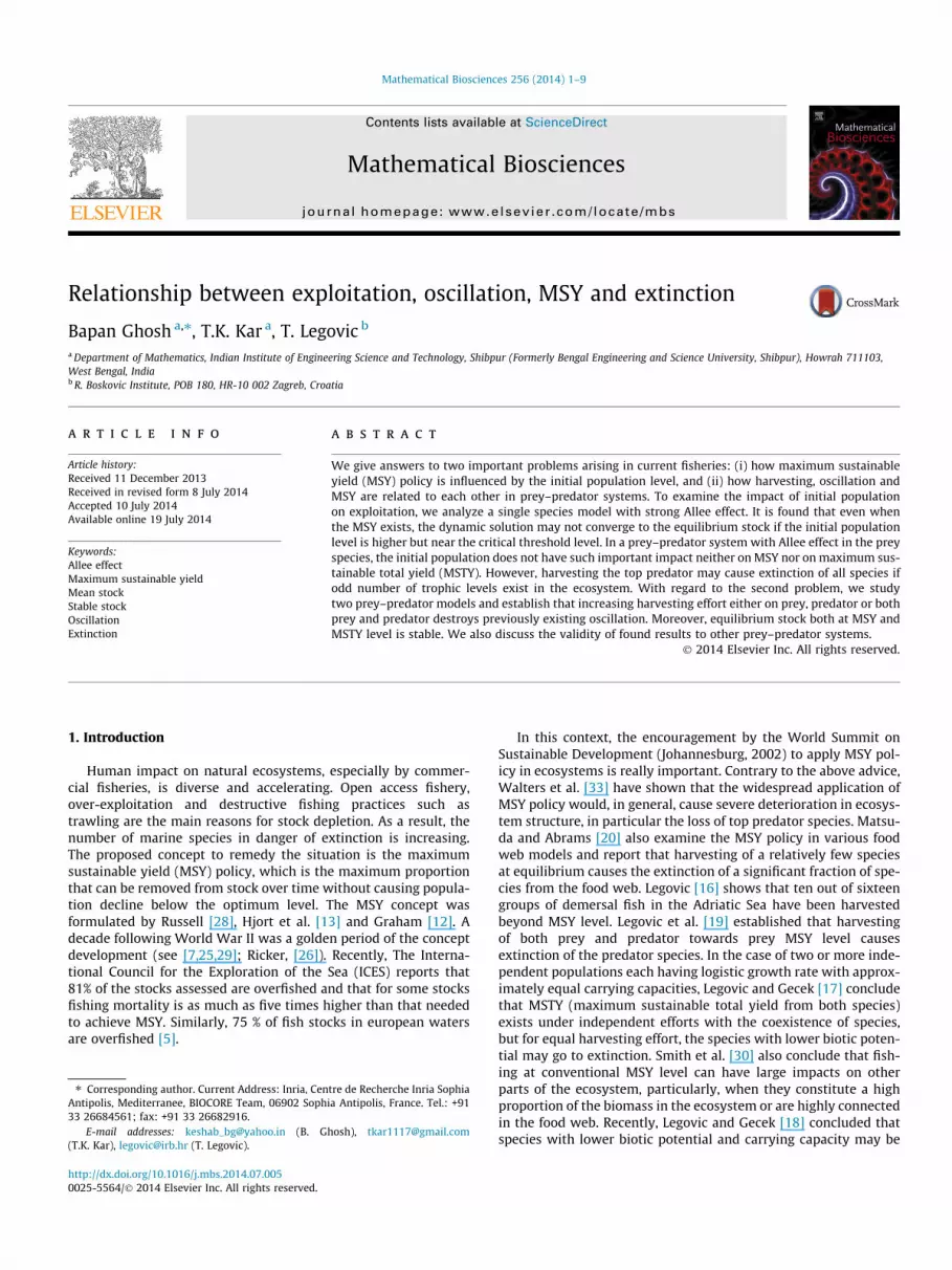
where x is the biomass of the concerned species at any time t > 0,while r and K are, respectively, the intrinsic growth rate and envi-ronmental carrying capacity of the species. The harvesting functionis taken as H ¼ qex, where q is the catchability coefficient and e isthe fishing effort. The single species model (2.1) has only one posi-tive equilibrium K in the absence of harvesting. The rate of growth(dx=dt) is positive if the initial population level is 0 < xðt ¼ 0Þ < K(see Fig. 1)a and negative if it is greater than K. Ultimately, thedynamic solution of the model converges to K for any xðt ¼ 0Þ > 0.
The positive equilibrium of the exploited system (2.1)x ¼ Kðr � qeÞ=r, exists if e < r=q.
The yield from the fishery at equilibrium becomesY ¼ ex ¼ Keðr � qeÞ=r.
Our aim is to achieve the maximum sustainable yield from thesystem (2.1). Since the yield function is quadratic in effort, it has asingle maximum at the equilibrium. MSY is obtained when theeffort is eMSY ¼ r=2q with equilibrium stock level xMSY ¼ K=2.Fig. 1b shows the variation in the biomass and the correspondingyield at the equilibrium.
Though MSY is taken at equilibrium for management purposes,the dynamic solution tends to xMSY from an initial population leveland will remain there for the long-term. In the present model, thedynamic solution converges globally to the equilibrium populationwhen harvesting reaches the MSY level. Hence MSY can beachieved in the single species model with logistic law of growth.In the following section, we show that this result may not holdfor the single species model in the presence of a strong Allee effect.
Remark 1. When the effort exceeds r=2q, the equilibrium stockbecomes less than K=2 and the species becomes over-harvested.But over-harvested species does not necessarily mean speciesextinction. If instead of proportional harvesting qex, a constantyield strategy is applied to the model (2.1), the zero equilibriumdisappears and a new unstable equilibrium exists. The value of thestable equilibrium is the same as that in constant effort strategyand the yield stays the same. The stable and unstable equilibriacoincide with each other at MSY = rK=4 and all dynamic solutionsreach MSY stock if initial population level exceeds K=2. But if thestock is overfished, i.e., 0 < x < K=2, then constant yield rK=4 willdrive the stock to extinction. No positive equilibrium can be foundif fishermen try to achieve higher yield than rK=4. In this case, themodel experiences a saddle node bifurcation for constant yieldstrategy.
3. MSY in the presence of an Allee effect
Let us consider a single species model (originally proposed byVolterra [32]) in the presence of an Allee effect (critical depensa-tion) and harvesting. The model is given by:
dxdt¼ rx 1� x
K
� � xL� 1
� �� qex; ð3:1Þ
where L (L < K) is the population level below which the populationwill tend to extinction.
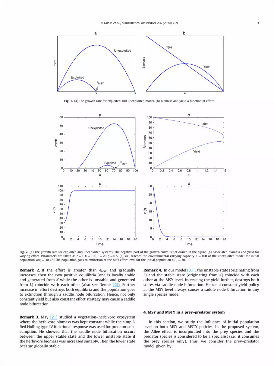
Fig. 2a shows the growth rate of the exploited and unexploitedsystems in the presence of a strong Allee effect. It is clear that theequilibrium population K of the unexploited system will be stableif the initial population level xð0Þ is greater than L ¼ 20. In the caseof harvesting, the initial population level xð0Þ must exceed 50 toobtain MSY. If the initial population level xð0Þ lies in the rangeð20;50Þ, then extinction of the population is evident at the MSYlevel. Hence an attempt to reach MSY may cause extinction ofthe population (see Fig. 2 c and d) even though the positive equi-librium exists at the effort required to achieve MSY. This phenom-enon will not occur in the logistic growth model. Since the successto achieve MSY also critically depends on the initial population,MSY may or may not exist in a single species model incorporatingthe strong Allee effect. In the present discussion, the minimum via-ble population should be greater than 50 for the existence of MSY.It is also clear that MSY occurs when the stock is at xMSY ¼ 70, andthe effort is eMSY ¼ 1:485. From Fig. 2a we observe that MSY occurswhen growth rate is the maximum and this maximum occurs forxMSY > K=2. In Fig. 2b the equilibrium stock and the correspondingyield are given as a function of effort
x
dx/d
t
xMSY
K
Exploited
Unexploited
a
e
Bio
mas
s
x(e)
Yield
b
Fig. 1. (a) The growth rate for exploited and unexploited model. (b) Biomass and yield a function of effort.
0 10 20 30 40 50 60 70 80 90 1000
10
20
30
40
50
60
x
dx/d
t
xMSYExploited
Unexploited
a
0 0.2 0.4 0.6 0.8 1 1.2 1.4 1.60
10
20
30
40
50
60
70
80
90
100
e
Bio
mas
s
x(e)
Yield
0 2 4 6 8 10 12 14 16 18 200
10
20
30
40
50
60
70
80
90
100
110
Time
x (t
)
c
0 2 4 6 8 10 12 14 16 18 200
5
10
15
20
25
30
Time
x (t
)
d
b
Fig. 2. (a) The growth rate for exploited and unexploited systems. The negative part of the growth curve is not drawn in the figure. (b) Associated biomass and yield forvarying effort. Parameters are taken as r ¼ 1;K ¼ 100; L ¼ 20; q ¼ 0:5. (c) xðtÞ reaches the environmental carrying capacity K ¼ 100 of the unexploited model for initialpopulation xð0Þ ¼ 30. (d) The population goes to extinction at the MSY effort level for the initial population xð0Þ ¼ 30.
B. Ghosh et al. / Mathematical Biosciences 256 (2014) 1–9 3
Remark 2. If the effort is greater than eMSY and graduallyincreases, then the two positive equilibria (one is locally stableand generated from K while the other is unstable and generatedfrom L) coincide with each other (also see Dennis [2]). Furtherincrease in effort destroys both equilibria and the population goesto extinction through a saddle node bifurcation. Hence, not onlyconstant yield but also constant effort strategy may cause a saddlenode bifurcation.
Remark 3. May [21] studied a vegetation–herbivore ecosystemwhere the herbivore biomass was kept constant while the simpli-fied Holling type IV functional response was used for predator con-sumption. He showed that the saddle node bifurcation occursbetween the upper stable state and the lower unstable state ifthe herbivore biomass was increased suitably. Then the lower statebecame globally stable.
Remark 4. In our model (3.1), the unstable state (originating fromL) and the stable state (originating from K) coincide with eachother at the MSY level. Increasing the yield further, destroys bothstates via saddle node bifurcation. Hence, a constant yield policyat the MSY level always causes a saddle node bifurcation in anysingle species model.
4. MSY and MSTY in a prey–predator system
In this section, we study the influence of initial populationlevel on both MSY and MSTY policies. In the proposed system,the Allee effect is incorporated into the prey species and thepredator species is considered to be a specialist (i.e., it consumesthe prey species only). Thus, we consider the prey–predatormodel given by:
0 0.2 0.4 0.6 0.8 1 1.2 1.4 1.6 1.80
5
10
15
20
25
30
35
40
45
50
e
Bio
mas
s
Predator
Yield
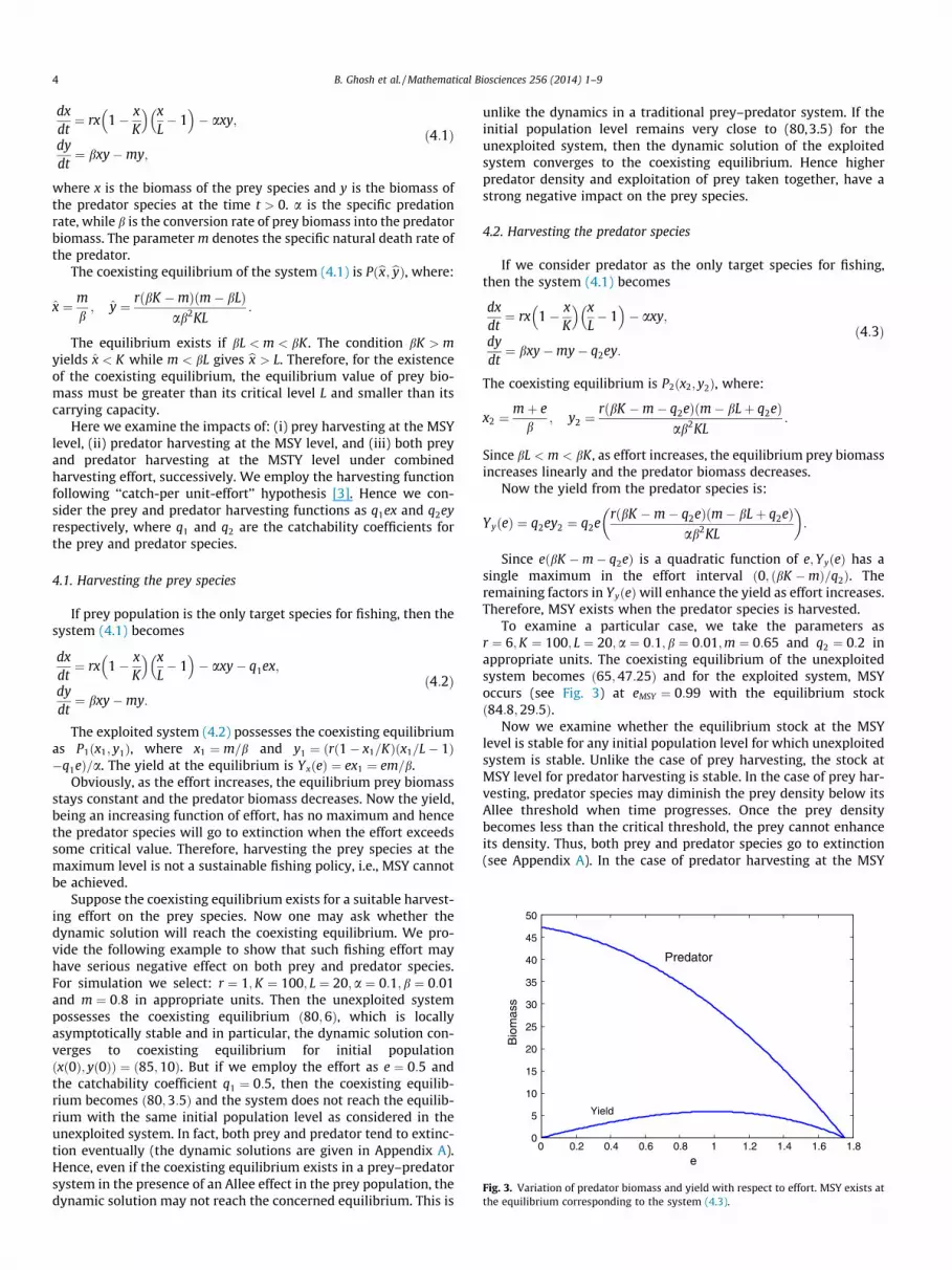
Fig. 3. Variation of predator biomass and yield with respect to effort. MSY exists atthe equilibrium corresponding to the system (4.3).
4 B. Ghosh et al. / Mathematical Biosciences 256 (2014) 1–9
dxdt¼ rx 1� x
K
� � xL� 1
� �� axy;
dydt¼ bxy�my;
ð4:1Þ
where x is the biomass of the prey species and y is the biomass ofthe predator species at the time t > 0. a is the specific predationrate, while b is the conversion rate of prey biomass into the predatorbiomass. The parameter m denotes the specific natural death rate ofthe predator.
The coexisting equilibrium of the system (4.1) is Pðbx; byÞ, where:
x ¼ mb; y ¼ rðbK �mÞðm� bLÞ
ab2KL:
The equilibrium exists if bL < m < bK. The condition bK > myields x < K while m < bL gives bx > L. Therefore, for the existenceof the coexisting equilibrium, the equilibrium value of prey bio-mass must be greater than its critical level L and smaller than itscarrying capacity.
Here we examine the impacts of: (i) prey harvesting at the MSYlevel, (ii) predator harvesting at the MSY level, and (iii) both preyand predator harvesting at the MSTY level under combinedharvesting effort, successively. We employ the harvesting functionfollowing ‘‘catch-per unit-effort’’ hypothesis [3]. Hence we con-sider the prey and predator harvesting functions as q1ex and q2eyrespectively, where q1 and q2 are the catchability coefficients forthe prey and predator species.
4.1. Harvesting the prey species
If prey population is the only target species for fishing, then thesystem (4.1) becomes
dxdt¼ rx 1� x
K
� � xL� 1
� �� axy� q1ex;
dydt¼ bxy�my:
ð4:2Þ
The exploited system (4.2) possesses the coexisting equilibriumas P1ðx1; y1Þ, where x1 ¼ m=b and y1 ¼ ðrð1� x1=KÞðx1=L� 1Þ�q1eÞ=a. The yield at the equilibrium is YxðeÞ ¼ ex1 ¼ em=b.
Obviously, as the effort increases, the equilibrium prey biomassstays constant and the predator biomass decreases. Now the yield,being an increasing function of effort, has no maximum and hencethe predator species will go to extinction when the effort exceedssome critical value. Therefore, harvesting the prey species at themaximum level is not a sustainable fishing policy, i.e., MSY cannotbe achieved.
Suppose the coexisting equilibrium exists for a suitable harvest-ing effort on the prey species. Now one may ask whether thedynamic solution will reach the coexisting equilibrium. We pro-vide the following example to show that such fishing effort mayhave serious negative effect on both prey and predator species.For simulation we select: r ¼ 1;K ¼ 100; L ¼ 20;a ¼ 0:1; b ¼ 0:01and m ¼ 0:8 in appropriate units. Then the unexploited systempossesses the coexisting equilibrium ð80;6Þ, which is locallyasymptotically stable and in particular, the dynamic solution con-verges to coexisting equilibrium for initial populationðxð0Þ; yð0ÞÞ ¼ ð85;10Þ. But if we employ the effort as e ¼ 0:5 andthe catchability coefficient q1 ¼ 0:5, then the coexisting equilib-rium becomes ð80;3:5Þ and the system does not reach the equilib-rium with the same initial population level as considered in theunexploited system. In fact, both prey and predator tend to extinc-tion eventually (the dynamic solutions are given in Appendix A).Hence, even if the coexisting equilibrium exists in a prey–predatorsystem in the presence of an Allee effect in the prey population, thedynamic solution may not reach the concerned equilibrium. This is
unlike the dynamics in a traditional prey–predator system. If theinitial population level remains very close to (80,3.5) for theunexploited system, then the dynamic solution of the exploitedsystem converges to the coexisting equilibrium. Hence higherpredator density and exploitation of prey taken together, have astrong negative impact on the prey species.
4.2. Harvesting the predator species
If we consider predator as the only target species for fishing,then the system (4.1) becomes
dxdt¼ rx 1� x
K
� � xL� 1
� �� axy;
dydt¼ bxy�my� q2ey:
ð4:3Þ
The coexisting equilibrium is P2ðx2; y2Þ, where:
x2 ¼mþ e
b; y2 ¼
rðbK �m� q2eÞðm� bLþ q2eÞab2KL
:
Since bL < m < bK, as effort increases, the equilibrium prey biomassincreases linearly and the predator biomass decreases.
Now the yield from the predator species is:
YyðeÞ ¼ q2ey2 ¼ q2erðbK �m� q2eÞðm� bLþ q2eÞ
ab2KL
� �:
Since eðbK �m� q2eÞ is a quadratic function of e;YyðeÞ has asingle maximum in the effort interval ð0; ðbK �mÞ=q2Þ. Theremaining factors in YyðeÞwill enhance the yield as effort increases.Therefore, MSY exists when the predator species is harvested.
To examine a particular case, we take the parameters asr ¼ 6;K ¼ 100; L ¼ 20;a ¼ 0:1; b ¼ 0:01;m ¼ 0:65 and q2 ¼ 0:2 inappropriate units. The coexisting equilibrium of the unexploitedsystem becomes ð65;47:25Þ and for the exploited system, MSYoccurs (see Fig. 3) at eMSY ¼ 0:99 with the equilibrium stockð84:8;29:5Þ.
Now we examine whether the equilibrium stock at the MSYlevel is stable for any initial population level for which unexploitedsystem is stable. Unlike the case of prey harvesting, the stock atMSY level for predator harvesting is stable. In the case of prey har-vesting, predator species may diminish the prey density below itsAllee threshold when time progresses. Once the prey densitybecomes less than the critical threshold, the prey cannot enhanceits density. Thus, both prey and predator species go to extinction(see Appendix A). In the case of predator harvesting at the MSY
35
40
45
50
Predator
B. Ghosh et al. / Mathematical Biosciences 256 (2014) 1–9 5
level, the growth rate of the predator species decreases and as aconsequence the prey density cannot decline below its Alleethreshold. Hence, a dynamic solution converges to the MSY stockwhen predator is exploited. From this view point also, predatorharvesting is a safe fishing policy.
0 0.2 0.4 0.6 0.8 1 1.2 1.4 1.6 1.80
5
10
15
20
25
30
e
Bio
mas
s
Yield
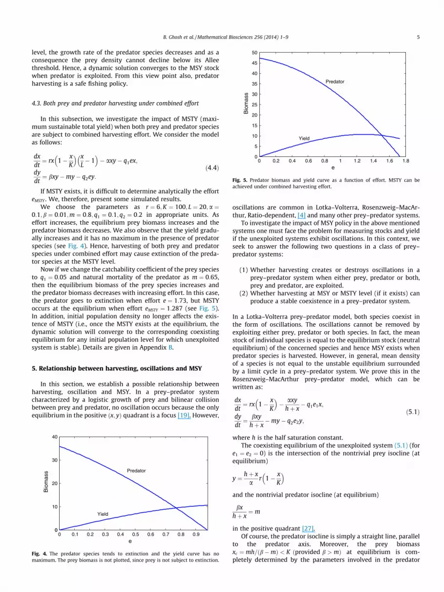
Fig. 5. Predator biomass and yield curve as a function of effort. MSTY can beachieved under combined harvesting effort.
4.3. Both prey and predator harvesting under combined effort
In this subsection, we investigate the impact of MSTY (maxi-mum sustainable total yield) when both prey and predator speciesare subject to combined harvesting effort. We consider the modelas follows:
dxdt¼ rx 1� x
K
� � xL� 1
� �� axy� q1ex;
dydt¼ bxy�my� q2ey:
ð4:4Þ
If MSTY exists, it is difficult to determine analytically the efforteMSTY . We, therefore, present some simulated results.
We choose the parameters as r ¼ 6;K ¼ 100; L ¼ 20;a ¼0:1; b ¼ 0:01;m ¼ 0:8; q1 ¼ 0:1; q2 ¼ 0:2 in appropriate units. Aseffort increases, the equilibrium prey biomass increases and thepredator biomass decreases. We also observe that the yield gradu-ally increases and it has no maximum in the presence of predatorspecies (see Fig. 4). Hence, harvesting of both prey and predatorspecies under combined effort may cause extinction of the preda-tor species at the MSTY level.
Now if we change the catchability coefficient of the prey speciesto q1 ¼ 0:05 and natural mortality of the predator as m ¼ 0:65,then the equilibrium biomass of the prey species increases andthe predator biomass decreases with increasing effort. In this case,the predator goes to extinction when effort e ¼ 1:73, but MSTYoccurs at the equilibrium when effort eMSTY ¼ 1:287 (see Fig. 5).In addition, initial population density no longer affects the exis-tence of MSTY (i.e., once the MSTY exists at the equilibrium, thedynamic solution will converge to the corresponding coexistingequilibrium for any initial population level for which unexploitedsystem is stable). Details are given in Appendix B.
5. Relationship between harvesting, oscillations and MSY
In this section, we establish a possible relationship betweenharvesting, oscillation and MSY. In a prey–predator systemcharacterized by a logistic growth of prey and bilinear collisionbetween prey and predator, no oscillation occurs because the onlyequilibrium in the positive ðx; yÞ quadrant is a focus [19]. However,
0 0.1 0.2 0.3 0.4 0.5 0.6 0.7 0.8 0.900
10
20
30
40
e
Bio
mas
s Predator
Yield
Fig. 4. The predator species tends to extinction and the yield curve has nomaximum. The prey biomass is not plotted, since prey is not subject to extinction.
oscillations are common in Lotka–Volterra, Rosenzweig–MacAr-thur, Ratio-dependent, [4] and many other prey–predator systems.
To investigate the impact of MSY policy in the above mentionedsystems one must face the problem for measuring stocks and yieldif the unexploited systems exhibit oscillations. In this context, weseek to answer the following two questions in a class of prey–predator systems:
(1) Whether harvesting creates or destroys oscillations in aprey–predator system when either prey, predator or both,prey and predator, are exploited.
(2) Whether harvesting at MSY or MSTY level (if it exists) canproduce a stable coexistence in a prey–predator system.
In a Lotka–Volterra prey–predator model, both species coexist inthe form of oscillations. The oscillations cannot be removed byexploiting either prey, predator or both species. In fact, the meanstock of individual species is equal to the equilibrium stock (neutralequilibrium) of the concerned species and hence MSY exists whenpredator species is harvested. However, in general, mean densityof a species is not equal to the unstable equilibrium surroundedby a limit cycle in a prey–predator system. We prove this in theRosenzweig–MacArthur prey–predator model, which can bewritten as:
dxdt¼ rx 1� x
K
� �� axy
hþ x� q1e1x;
dydt¼ bxy
hþ x�my� q2e2y;
ð5:1Þ
where h is the half saturation constant.The coexisting equilibrium of the unexploited system (5.1) (for
e1 ¼ e2 ¼ 0) is the intersection of the nontrivial prey isocline (atequilibrium)
y ¼ hþ xa
r 1� xK
� �and the nontrivial predator isocline (at equilibrium)
bxhþ x
¼ m
in the positive quadrant [27].Of course, the predator isocline is simply a straight line, parallel
to the predator axis. Moreover, the prey biomassxc ¼ mh=ðb�mÞ < K ðprovided b > mÞ at equilibrium is com-pletely determined by the parameters involved in the predator

6 B. Ghosh et al. / Mathematical Biosciences 256 (2014) 1–9
growth. On the other hand, prey isocline is a quadratic function of xand possesses a maximum when
x ¼ xM ¼12
K � hð Þ:
If the prey-biomass xc at the coexisting equilibrium is higher thanxM , then both species posses globally stable coexistence, otherwisethe system exhibits a globally stable limit cycle [1]. Without anyloss of generality and in the absence of harvesting, we suppose thatboth species coexist in the form of oscillations (i.e., xc < xM) (seeFig. 6). We now discuss following three cases:
(i) whether prey harvesting (e1 > 0; e2 ¼ 0) destroys oscillationin a Rosenzweig MacArthur model. Under prey exploitation,the prey biomass (xc) remains constant and the predator iso-cline possesses a maximum when
Fig. 6.isoclineunexplodestroy
x ¼ xe1M ¼
12
Kð1� q1e1
rÞ � h
� �:
As effort e1 increases, xe1M moves towards the left on the prey axis x
whereas xc remains at the same place. Increasing effort makesxe1
M < xc < xM (see Fig. 6). This reveals that harvesting the prey spe-cies destroys oscillations and can produce a stable coexistence.Since the prey biomass is independent of effort, the yield increaseslinearly with effort. Hence the predator species goes to extinction inorder to achieve MSY from the prey species.
(ii) In the case of predator harvesting (e1 ¼ 0; e2 > 0), as effort e2
increases, xM remains fixed, but xe2c ¼ hðmþ q2e2Þ=ðb�m�
q2e2Þ moves to the right on the prey axis x. Hence, oscilla-tions can be removed with the increasing harvesting efforton the predator species. A sufficiently large effort can yieldxM < xe2
c to produce a stable coexistence in the Rosen-zweig–MacArthur model.As a sufficiently large effort on predator species produces astable coexistence, one may ask whether the effort at theMSY is sufficiently large. Alternatively, we examine whetherstocks at the MSY level of predator harvesting are found in astable equilibrium. The coexisting equilibrium for predatorharvesting is
ðxe2 ;ye2Þ¼ hðmþq2e2Þ
b�m�q2e2;
hrb Kðb�mÞ�hm�ðKþhÞq2e2ð ÞKaðb�m�q2e2Þ
� �:
ð5:2Þ
00
Prey biomass
Pre
dato
r bi
omas
s
xM
xcxMe
1
Prey isocline for unexploited systemPrey isocline for exploited system
Relative position of xc with respect to the peak (maximum) of the preys in the exploited and unexploited Rosenzweig–MacArthur model. Theited system exhibits oscillation for xc < xM . But prey exploitation canoscillations when xe1
M < xc .
Obviously this equilibrium is unstable for smaller effort e2.The yield at the equilibrium is
Table 1Meanoscillati
EfforMeaMeaMeaUnstUnst
Yðe2Þ ¼ q2e2ye2
¼ q2e2hrb Kðb�mÞ � hm� ðK þ hÞq2e2ð Þ
Kaðb�m� q2e2Þð5:3Þ
and it would be the maximum when
e2 ¼ðb�mÞ Kðb�mÞ � hmð Þq2 Kðb�mÞ � hmþ 2hbð Þ
with the prey biomass
xMSY ¼12
K þ hmb�m
� �:
Since xM < xMSY , the predator stock at MSY experiences a stablecoexistence.The above MSY may not be unique MSY as we have calculated theyield by taking the unstable equilibrium ðxe2 ; ye2
Þ. Therefore, welook whether there exists another MSY for increasing effort bydetermining the mean stock. For simulation purpose, we selectr ¼ 1;K ¼ 50;a ¼ 0:3;b ¼ 0:3; h ¼ 5;m ¼ 0:1. Then, the prey bio-mass xc ¼ 2:5, the predator biomass yc ¼ 23:75 and xM ¼ 22:5. Asxc is very small compared to xM , the equilibrium is unstable and itis surrounded by a globally stable limit cycle. Supposeq2 ¼ 0:1455 (to normalize effort), then the system becomes stablewhen e2 ¼ 1. At the MSY level, the stable equilibrium becomesð26:25;49:48Þ with the yield of 7.51. The following Table 1 repre-sents the mean density of both prey and predator species forincreasing effort in the interval ð0;1Þ.From Table 1, it is clear that the unstable equilibrium is not equal tothe mean stock. In addition, both the unstable equilibrium stockand the mean predator stock increase with increasing effort. Thisimplies that by harvesting the predator species, the mean yieldhas no maximum and hence the expressions (5.2) and (5.3) giveunique and stable MSY.
(iii) When we consider the case of equal effort (i.e., e1 ¼ e2 ¼ e)on both species, as effort increases we find that it shiftsthe peak of the prey isocline to the left and the predator iso-cline to the right along the prey axis. Hence, by increasingthe effort on both species ultimately eliminates oscillationfrom the system and a stable coexistence can be found.
With a suitable choice of q1 and q2, one can reach MSTY. DoesMSTY (if it exists) make the equilibrium stable? Yes it does. Sincethe yield from the prey biomass does not posses a maximum,predator must be over-exploited to achieve the MSTY. In addition,when the predator is harvested, the coexisting equilibrium isstable at the MSY, hence it remains stable even when the predatoris over-exploited. Moreover, we know that harvesting the preyspecies cannot create oscillations in a previously existing stablesystem. Therefore, we conclude that the equilibrium at the MSTYlevel is stable.
To investigate the answer of our questions further, we considerthe prey–predator system given by:
density of both species when Rosenzweig–MacArthur model exhibitson.
t 0.4 0.6 0.8 0.9 0.95 0.98 0.999n (x) 24.20 28.58 32.64 34.03 33.60 26.75 22.54n (y) 18.19 19.00 20.76 23.12 26.56 40.45 50.26n yield 1.06 1.66 2.42 3.03 3.67 5.77 7.30able x 5.58 8.31 12.94 16.72 19.28 21.13 22.45able y 31.33 36.99 44.43 48.83 50.00 50.22 50.42

B. Ghosh et al. / Mathematical Biosciences 256 (2014) 1–9 7
dxdt¼ rx 1� x
K
� � xL� 1
� �� axy
hþ x� q1e1x;
dydt¼ bxy
hþ x�my� q2e2y:
ð5:4Þ
In the model, oscillations may occur in the absence of harvest-ing [34]. We now show that the above results also hold for the sys-tem (5.4). The highest peak of the prey isocline (at the equilibrium)of the unexploited system (5.4) is
x ¼ xM ¼ðK þ L� hÞ þ
ffiffiffiffiffiffiffiffiffiffiffiffiffiffiffiffiffiffiffiffiffiffiffiffiffiffiffiffiffiffiffiffiffiffiffiffiffiffiffiffiffiffiffiffiffiffiffiffiffiffiffiffiffiffiffiffiffiffiffiffiffiffiffiffiffiffiffiffiðK þ L� hÞ2 þ 3ððK þ LÞh� KLÞ
q3
:
Prey biomass xc would be same in the system (5.4) as predatorgrowth rates are the same in both models. Likewise, in the Rosen-zweig–MacArthur model, both prey and predator of the system(5.1) coexist in the form of oscillations1 if x] < xc < xM (for moredetails see [34]).
Now we examine whether oscillations and MSY exist in thesystem (5.4) for different harvesting schemes.
(i) Suppose an unexploited system possesses a stable limitcycle for x] < xc < xM . If only prey is harvested (e2 ¼ 0), thenxc remains fixed, but the peak of the prey isocline would be
1 Heroscillatireader c
x¼ xe1M
¼ðKþL�hÞþ
ffiffiffiffiffiffiffiffiffiffiffiffiffiffiffiffiffiffiffiffiffiffiffiffiffiffiffiffiffiffiffiffiffiffiffiffiffiffiffiffiffiffiffiffiffiffiffiffiffiffiffiffiffiffiffiffiffiffiffiffiffiffiffiffiffiffiffiffiffiffiffiffiffiffiffiffiffiffiffiffiffiffiffiffiffiffiffiffiffiðKþL�hÞ2þ3ððKþLÞh�KL�q1e1KL=r2Þ
q3
:
Obviously xe1M < xM for any effort on prey species. This revels that
increasing harvesting effort can make xe1M < xM < xc , which results
in a stable coexistence of both species. Hence, prey harvesting inthe system (5.4) has the same effect we have observed in the Rosen-zweig–MacArthur model. As the prey biomass remains constantwhen prey is harvested, no MSY exists.
(ii) From the result in the Rosenzweig–MacArthur model it is astraight forward to prove that the predator harvestingdestroys oscillations and a suitable effort can produce stablecoexistence in the system (5.4). It is difficult to show analyt-ically that stocks at the MSY level for predator harvesting arestable. We give an example to discuss this issue using theparameters as: r ¼ 1;K ¼ 1; L ¼ 0:4;a ¼ 1:693; b ¼ 1:693;h ¼ 0:5;m ¼ 1 (parameters are taken from [34]). For thisparameter set, the system possesses a stable limit cycle sur-rounding the unstable equilibrium ð0:7215;0:1615Þ togetherwith xM ¼ 0:73589. If we choose q2 ¼ 0:0798 (to normalizethe effort at MSY), the limit cycle disappeared for a verysmall effort e2 ¼ 0:1 and we have the stable stockð0:88;0:117Þ at MSY for e2 ¼ 1.
(iii) Likewise the Rosenzweig–MacArthur model, one can easilyfind that harvesting of both species can remove oscillationsand if MSTY exists it becomes a stable equilibrium.
In discussion and conclusion section we mention whether ourresults are expected to be valid in other prey–predator systems.
Remark 5. We have not analyzed any oscillation scenarios forspecies exploitation in the model (4.1). The oscillation may occureven in the presence of bilinear collision of prey and predator. Inthe Rosenzweig–MacArthur model and in the unexploited system(5.4), oscillations occur when the equilibrium prey biomass xc
remains in ð0; xMÞ and ðx]; xMÞ, respectively. Hence, smaller
e x] is a critical value of x, and it is found at the lower range of x for whichons occurs. We do not explicitly calculate the value of x] , but the interestedan find it in [34].
harvesting effort does not remove oscillations from the systems(5.1) and (5.4). On the other hand, [14] have pointed out thatoscillations occur in system (4.1) only when the prey biomass xc isðK þ LÞ=2 at the equilibrium. Therefore, any smaller harvestingeffort on either species can remove the oscillation from the system(4.1).
6. Discussion and conclusion
In this study, the convergence of the dynamic solutions to equi-librium stock is examined in both single species and prey–predatorexploited models. Any dynamic solution converges globally to theexploited stock in single species logistic growth model. This resultindicates that any dynamic solution always converges globally tothe coexisting stock in a traditional prey–predator system [19].Moreover, if the coexisting equilibrium exists in the Rosenzweig–MacArthur model, then dynamic solutions converge globally eitherto the coexisting equilibrium or to a stable limit cycle (thishappens when coexisting equilibrium is unstable). Hence, the exis-tence of the interior equilibrium under proportional harvesting(CPUE harvest strategy) guarantees the persistence of both speciesin the long run.
In the case of a single species model incorporating strong Alleeeffect, MSY exists at the equilibrium, but the dynamic solution maynot reach the MSY stock in the long run. This represents a signifi-cant difference in harvesting results between a traditionalprey–predator system and the system (4.1). In a traditional, theRosenzweig–MacArthur and many other classes of models [19,Eqs. (19) and (20)], the equilibrium prey biomass (determined bythe parameters involved in predator growth function only) remainsconstant and predator biomass decreases for increasing harvestingrate on prey species. In this case, dynamic solutions always con-verge to the coexisting equilibrium. Of course, variation of theequilibrium biomass of both prey and predator for the system(4.2) is similar to the traditional prey–predator system for increas-ing effort, but the prey growth rate may decrease significantly dueto consumption by the higher trophic level. As a consequence, thepredator species may produce a negative effect on the prey growthrate. The dynamic solution of the prey species may reach a valuebelow its critical threshold level (L) and both species tend toextinction. On the other hand, harvesting the predator species atthe MSY level reduces its growth rate and no additional negativeeffect occurs on the prey growth rate. Hence, predator harvestingdoes not cause extinction. Likewise, if MSTY exists at the equilib-rium then dynamic solutions reach the corresponding stock. Onemay ask whether the predator harvesting to MSY is a safe harvest-ing policy from extinction viewpoint as suggested by [22,19,9]. InAppendix C, we have shown that harvesting the top predator atthe MSY level may cause extinction of all the trophic levels.
It is well known that fluctuating environment and ecologicalbehavior of species may create oscillations, hence it is importantto analyze whether harvesting may cause oscillations in fishery.In this context, we have studied impact of exploitation on theRosenzweig–MacArthur model in which species coexist and oscil-late. It is established that increasing harvesting rate either on prey,predator or both species destroys oscillations in the system. There-fore, if an unexploited system is in a stable state, then harvestingnever creates oscillations in the Rosenzweig–MacArthur modeland in such a situation one may easier estimate the yield and thestock at MSY or MSTY level. On the other hand, if the system exhib-its oscillations, then one needs to calculate the mean stock for bothprey and predator species. In the Rosenzweig–MacArthur model,by increasing the harvesting rate on predator species enhancesits mean stock and hence MSY does not exist when the system isin oscillation. This indicates that MSY for predator harvesting can

0 50 100−10
0
10
20
30
40
50
60
70
80
90
Time
Pre
y
0 50 100−2
0
2
4
6
8
10
12
Time
Pre
dato
r
Fig. A2. Both prey and predator species go to extinction in the exploited system(4.2) for the initial population level ð85;10Þ.
60
8 B. Ghosh et al. / Mathematical Biosciences 256 (2014) 1–9
be achieved only if the system is in a stable equilibrium. We alsoprove that the stock at MSTY is also in a stable equilibrium. Wehave shown that all the above principles are valid in the system(5.4) and one can verify that these principles can also be appliedto [4] prey–predator model.
Therefore, one may think that harvesting never causes oscilla-tions in a prey–predator system. Actually, prey harvesting maycause oscillations in a ratio-dependent system, as it has beenshown by [35]. In the same example, we have shown that nooscillations occur when MSY is reached (see Appendix D). Thoughin another example it is observed that oscillations exist when theprey species is harvested to MSY. In addition, it is also observedthat oscillation can be destroyed if predator is exploited in aratio-dependent system (see the Appendix D). In conclusion, wemay state that oscillatory phenomenon under exploitation mostlydepends upon the predator functional response (based on Hollingtype or ratio-dependent).
In a prey–predator system, we now conclude that prey harvest-ing is detrimental as it may cause either (i) extinction of predator,(ii) extinction of both prey and predator or (ii) oscillations. On theother hand, predator harvesting is free from these detrimentaleffects.
10
20
30
40
50P
reda
tor
R1
R2
R3
AcknowledgementsB. G. is financed by the Council of Scientific and IndustrialResearch (CSIR), India (File No. 08/003(0077)/2011-EMR-I, dated25th April, 2013); T.K. Kar is supported by the University GrantsCommission (UGC), India (F. No. 40-239/2011(SR), dated 29th June,2011) and T.L. is financed by the Croatian Ministry for Science,Education and Sports. The authors are grateful to the anonymousreferees for providing a number of important insights andsuggestions.
20 30 40 50 60 70 80 90 1000
Prey
Fig. B1. Stability region of the exploited system (4.1) and the unexploited system(4.4) corresponding to the coexisting equilibrium.
Appendix A
Fig. A1 shows that the coexisting equilibrium ð80;6Þ of theunexploited system (4.1) is asymptotically stable for the initialpopulation level ð85;10Þ, while Fig. A2 shows that the coexistingequilibrium of the exploited system (4.2) is stable at the originfor the same initial population level ð85;10Þ.
0 50 10060
65
70
75
80
85
Time
Pre
y
0 50 1005.5
6
6.5
7
7.5
8
8.5
9
9.5
10
10.5
Time
Pre
dato
r
Fig. A1. Time response of the prey and the predator species of the unexploitedsystem (4.1) for the initial population level ð85;10Þ.
Appendix B
Fig. B1 shows that the region R1 is an attractor for the coexistingequilibrium � of the unexploited system (4.1). R1
SR2 is an attrac-
tor for the coexisting equilibrium I of the exploited system (4.4).As R1 is contained in R1
SR2, the dynamic solutions will reach
MSTY stock for any initial population level in R1.
Appendix C
We consider a food chain with three trophic levels: prey–pred-ator-top predator. The model is given by:
dxdt¼ rx 1� x
K
� � xL� 1
� �� axy
dydt¼ bxy� cyz�my
dxdt¼ lyz� nz� q3e3z;
where z is the top predator, c and l are, respectively, the predationand conversion coefficients for the consumption process by the toppredator on the first predator y. n is the specific natural mortalityrate of z. e3 is the effort on the predator with the catchabilitycoefficient q3.
B. Ghosh et al. / Mathematical Biosciences 256 (2014) 1–9 9
If we select r ¼ 2;K ¼ 100; L ¼ 20;a ¼ 0:2; b ¼ 0:025;m ¼ 0:6c ¼ 0:3;l ¼ 0:03 and n ¼ 0:2, then the coexisting equilibriumbecomes ð76:3;6:7;4:4Þ. The dynamic solution converges to theequilibrium for the initial condition ðxð0Þ; yð0Þ; zð0ÞÞ ¼ ð35;6;4Þ.In this case we take smaller initial prey population compared tothe equilibrium stock. When the top predator is exploited to theMSY, all the species tend to extinction. Actually, harvesting thetop predator decreases its growth rate, which results in an increasein the growth rate of the first predator when time progresses.Increasing the growth rate of the first predator ultimately causesa negative effect on the growth rate of the prey species. Ultimatelythe prey species decreases below its critical threshold L and all thespecies tend to extinction. In general, harvesting the top trophiclevel in a system with 2N (where N P 1 is an integer) predatortrophic levels may have a negative effect on the persistence of alltrophic levels. However, for a food chain with odd number ofpredator trophic levels ð2N � 1Þ this may not be the case.
Appendix D
A ratio-dependent prey–predator model in the presence ofharvesting is given by:
dxdt¼ rx 1� x
k
� �� cxy
myþ x� hx;
dydt¼ sxy
myþ x� dy� ey:
The meanings of the ecological parameters in the above modelare available in [35]. Here h and e are the harvesting efforts on theprey and the predator species, respectively. Xiao and Cao [35] haveshown that the unexploited system is stable at the coexisting equi-librium if r ¼ 1; k ¼ 1; c ¼ 1:3; s ¼ 0:8 and d ¼ 0:4, and that it startsto oscillate if only the prey species is exploited with efforth ¼ 0:225. In this particular parameter setting, we observe thatMSY is a stable state for the effort h ¼ hMSY ¼ 0:175. However, ifwe select r ¼ 0:8 and k ¼ 0:8, oscillations would occur if one har-vests the prey population to MSY. Therefore, an attempt to reachMSY by harvesting the prey species in a ratio-dependent systemmay not produce a stable coexistence. The unexploited systemwould become oscillatory for r ¼ 0:768 and k ¼ 0:768 (whichyields exactly the same Fig. 4 in [35]), but in this case predator har-vesting to the MSY level produces a stable coexistence.
References
[1] G.J. Butler, P. Waltman, Bifurcation from a limit cycle in a two predator-oneprey ecosystem modeled on a chemostat, J. Math. Biol. 12 (1981) 295–310.
[2] B. Dennis, Allee effects: population growth, critical density, and the chance ofextinction, Nat. Resour. Model. 3 (4) (1989) 481–538.
[3] C.W. Clark, Mathematical Bioeconomics: The Optimal Management ofRenewable Resources, second ed., Wiley, New York, 1990.
[4] D.L. DeAngelis, R.A. Goldstein, R.V. O’Neill, A model for trophic interaction,Ecology 56 (1975) 881–892.
[5] EU, CFP Reform – Maximum Sustainable Yield, 2013 <http://ec.pa.eu/fisheries/reform/docs/msy_en.pdf>.
[6] J.D. Flores, E.G. Olivares, Dynamics of a predator–prey model with Allee effecton prey and ratio-dependent functional response, Ecol. Complex (2014) http://dx.doi.org/10.1016/j.ecocom.2014.02.005.
[7] F.E.J. Fry, Statistics of a lake trout fishery, Biometrics 5 (1947) 27–67.[8] S. Gecek, T. Legovic, Impact of maximum sustainable yield on competitive
community, J. Theoret. Biol. 307 (2012) 96–103.[9] B. Ghosh, T.K. Kar, Possible ecosystem impacts of applying maximum
sustainable yield policy in food chain models, J. Theoret. Biol. 329 (2013) 6–14.[10] B. Ghosh, T.K. Kar, Maximum sustainable yield and species extinction in a
preypredator system: some new results, J. Biol. Phys. (2013), http://dx.doi.org/10.1007/s10867-013-9303-2.
[11] B. Ghosh, T.K. Kar, Sustainable use of ecosystem services: jointly determinedecological thresholds and economic trade-offs, Ecol. Model. 272 (2014) 4958.
[12] M. Graham, Modern theory of exploiting a fishery, an application to North seatrawling, J. Con. Int. 1’Expl. Mer 10 (1935) 264–274.
[13] J. Hjort, G. Jahn, P. Ottestad, The optimum catch, Hvalradets Skrifter 7 (1933)92–127.
[14] T.K. Kar, H. Matsuda, Sustainable management of a fishery with a strong Alleeeffect, Trends Appl. Sci. Res. 2 (4) (2007) 271–283.
[15] T.K. Kar, B. Ghosh, Impacts of maximum sustainable yield policy to prey–predator systems, Ecol. Model. 250 (2013) 134–142.
[16] T. Legovic, Impact of demersal fishery and evidence of the Volterra principle tothe extreme in the Adriatic Sea, Ecol. Model. 212 (2008) 68–73.
[17] T. Legovic, S. Gecek, Impact of maximum sustainable yield on independentpopulations, Ecol. Model. 221 (2010) 2108–2111.
[18] T. Legovic, S. Gecek, Impact of maximum sustainable yield on mutualisticcommunities, Ecol. Model. 230 (2012) 63–72.
[19] T. Legovic, J. Klanjscek, S. Gecek, Maximum sustainable yield and speciesextinction in ecosystems, Ecol. Model. 221 (2010) 1569–1574.
[20] H. Matsuda, P.A. Abrams, Maximal yields from multispecies fisheries systems:rules for systems with multiple trophic levels, Ecol. Appl. 16 (2006) 225–237.
[21] R.M. May, Thresholds and breakpoints in ecosystems with a multiplicity ofstable states, Nature 269 (1977) 471–477.
[22] R.M. May, J.R. Beddington, C.W. Clark, S.J. Holt, R.M. Laws, Management ofmultispecies fisheries, Science 205 (1979) 267–277.
[23] E.G. Olivares, J.M. Lorca, A.R. Palma, J.D. Flores, Dynamical complexities in theLeslie–Gower prey–predator model as consequences of the Allee effect onprey, Appl. Math. Model. 35 (2011) 366–381.
[24] A.J. Palma, E.G. Olivares, Optimal harvesting in a prey–predator model withAllee effect and sigmoidal functional response, Appl. Math. Model. 36 (2011)1864–1874.
[25] W.E. Ricker, Methods of Estimating Vital Statistics of Fish Populations, IndianaUniv. Publ. Sci. Ser., 1948.
[26] W.E. Ricker, 1968. Handbook of Computations for Biological Statistics of FishPopulations, Bull. 119, Fish. Res. Board Can, Ottawa.
[27] M.L. Rosenzweig, R.H. MacArthur, Graphical Representation and stabilityconditions of predator–prey interactions, Am. Natural. 97 (1963) 209–223.
[28] E.S. Russell, Some theoretical considerations of ’overfishing’ problem, J. Con.Int. 1’Expl. Mer 6 (1931) 1–20.
[29] M.B. Schaefer, Some aspects of the dynamics of populations important to themanagement of commercial marine fisheries, Bullet. Inter-Am. Trop. TunaComm. 1 (1954) 25–56.
[30] A.D.M. Smith, C.J. Brown, C.M. Bulman, E.A. Fulton, P. Johnson, I.C. Kaplan, H.L.Montes, S. Mackinson, M. Marzloff, L.J. Shannon, Y.J. Shin, J. Tam, Impacts offishing low-trophic level species on marine ecosystems, Science 333 (2011)1147–1150.
[31] P.A. Stephens, W.J. Sutherland, Consequences of the Allee effect for behavior,ecology and conservation, TREE 14 (10) (1999) 401–405.
[32] V. Volterra, Population growth, equilibria, and extinction under specifiedbreeding conditions: a development and extension of logistic curve, Hun. Biol.3 (1938) 1–11.
[33] C.J. Walters, V. Christensen, S.J. Martell, J.F. Kitchell, Possible ecosystemimpacts of applying MSY policies from single-species assessment, ICES J.Marine Sci. 62 (2005) 558–568.
[34] J. Wang, J. Shi, J. Wei, Predator–prey system with strong Allee effect in prey, J.Math. Biol. 62 (2011) 291–331.
[35] M. Xiao, J. Cao, Hopf bifurcation and non-hyperbolic equilibrium in a ratio-dependent predator–prey model with linear harvesting rate, Math. Comp.Model. 50 (2009) 360–379.