the forcing of the pacific decadal oscillation*

The Forcing of the Pacific Decadal Oscillation*

NIKLAS SCHNEIDER

International Pacific Research Center, and Department of Oceanography, University of Hawaii at Manoa, Honolulu, Hawaii

BRUCE D. CORNUELLE

Scripps Institution of Oceanography, University of California, San Diego, La Jolla, California

(Manuscript received 3 August 2004, in final form 19 April 2005)

ABSTRACT

The Pacific decadal oscillation (PDO), defined as the leading empirical orthogonal function of NorthPacific sea surface temperature anomalies, is a widely used index for decadal variability. It is shown that thePDO can be recovered from a reconstruction of North Pacific sea surface temperature anomalies based ona first-order autoregressive model and forcing by variability of the Aleutian low, El Niño–Southern Oscil-lation (ENSO), and oceanic zonal advection anomalies in the Kuroshio–Oyashio Extension. The latterresults from oceanic Rossby waves that are forced by North Pacific Ekman pumping. The SST responsepatterns to these processes are not orthogonal, and they determine the spatial characteristics of the PDO.The importance of the different forcing processes is frequency dependent. At interannual time scales,forcing from ENSO and the Aleutian low determines the response in equal parts. At decadal time scales,zonal advection in the Kuroshio–Oyashio Extension, ENSO, and anomalies of the Aleutian low eachaccount for similar amounts of the PDO variance. These results support the hypothesis that the PDO is nota dynamical mode, but arises from the superposition of sea surface temperature fluctuations with differentdynamical origins.

1. Introduction

The Pacific decadal oscillation (PDO) index (Mantuaet al. 1997) is widely used to characterize North Pacificdecadal variability and anomalies of Northern Hemi-sphere climate and the North Pacific ecosystem. Yet,the processes underlying the temporal and spatial char-acteristics of the PDO have not been clarified. Here, wepresent a statistical analysis of North Pacific sea surfacetemperature (SST), sea level pressure (SLP), andwind stress to identify the drivers of the PDO and theirrelative contributions to its temporal and spatialpatterns.

The PDO is defined1 as the leading empirical or-thogonal function (EOF) of monthly anomalies (devia-tions from the climatological annual cycle) of sea sur-face temperature in the Pacific poleward of 20°N(Davis 1976; Mantua et al. 1997). Its temporal evolution(Fig. 1) is marked by variability on interannual anddecadal time scales, with several pronounced shifts—the 1976/77 transition being the most famous and ex-tensively studied (Trenberth 1990; Graham 1994; Tren-berth and Hurrell 1994; Miller et al. 1994). The spatialpattern of the PDO (Fig. 2) resembles a horseshoe, withtemperature anomalies in the central North Pacific sur-rounded by anomalies of opposite sign in the Alaskagyre, off California, and toward the Tropics.

* International Pacific Research Center Contribution Number335 and School of Ocean and Earth Science and Technology Con-tribution Number 6594.

Corresponding author address: N. Schneider, IPRC, Universityof Hawaii at Manoa, 1680 East West Road, Honolulu, HI 96822.E-mail: [email protected]

1 In the original definition of the PDO, the global monthlymean SST anomaly is removed prior to the calculation of theEOF. The leading EOF of this field and of the raw monthly SSTanomalies is barely different, and we consider the raw SSTanomalies. This is dictated by our desire to develop a regressionmodel for the North Pacific SST anomalies, without attempting asimilar model for the global mean of the SST.

1 NOVEMBER 2005 S C H N E I D E R A N D C O R N U E L L E 4355

© 2005 American Meteorological Society

JCLI3527

The PDO and its associated sea level pressure patternhave attracted considerable attention because their timeevolutions are correlated with anomalies of the Pacificecosystem (Mantua et al. 1997); North American precipi-tation, streamflow, and surface temperature anomalies(Mantua and Hare 2002; Dettinger et al. 1998; Cayanet al. 1998); surface temperature anomalies in north-eastern Asia (Minobe 2000); fluctuations of the Asianmonsoon (Krishnan and Sugi 2003); and a modulationof El Niño–Southern Oscillation (ENSO) teleconnec-tions (Gershunov and Barnett 1998). This covariationcan result from the PDO forcing the atmosphere orfrom a common forcing of the PDO and covarying cli-mate anomalies. Model experiments suggest the latterexplanation for the decadal modulation of ENSO tele-connections (Pierce 2002). However, this question hasnot been clarified from observations, and requires theidentification of the forcing mechanism of the PDO.

The PDO pattern is qualitatively consistent with theatmospheric forcing associated with fluctuations of po-sition and strength of the Aleutian low. In the centralNorth Pacific, a deepened Aleutian low decreases SSTby advection of cool and dry air from the north, byincreases of westerly winds and ocean-to-atmosphereturbulent heat fluxes, and by strengthened equatorwardadvection of temperature by Ekman currents. In theeastern regions, a deepened Aleutian low enhancespoleward winds and leads to warm anomalies of surfacetemperature.

However, this qualitative picture hides the complexprocesses governing changes of the Aleutian low andNorth Pacific SST anomalies. The North Pacific atmo-sphere affects the surface heat budget via anomalies ofsurface fluxes and Ekman advection (Alexander 1992),and the excitation and propagation of Rossby wavesthat affect the upper ocean in the Kuroshio–OyashioExtension (KOE) region (Miller et al. 1998; Deser et al.1999; Xie et al. 2000; Miller and Schneider 2000; Seageret al. 2001; Schneider et al. 2002; Qiu 2003). The

FIG. 1. Time series of monthly values of (from the top) thePDO, Niño-3.4, NPI, PDEL, and PAVG. All time series are nor-malized to unit standard deviation. The thick line overlaid on thetop curve shows the PDO based on Jul–Jun annual averages ofSSTA. The correlation of annual averages of the monthly valuesof the PDO, and of the PDO estimated from annual averages ofSSTA, is 0.99, and the latter is used in this study. The dotted linesoverlaid on the lower two curves denote PDEL and PAVG obtainedfrom North Pacific wind stress curl that had the regression withlow-pass time series of Niño-3.4 and NPI removed.

FIG. 2. (top) PDO pattern from observations, (middle) derivedas the leading EOF of the reconstructed SSTA, and (bottom)derived from the reconstruction obtained with a spatially constantvalue of �. The magnitude depicts the SSTA (K) for a unit de-viation of the principal component; the contour level is 0.2, withnegative contours dotted.

4356 J O U R N A L O F C L I M A T E VOLUME 18

anomalies of the atmosphere reflect its intrinsic vari-ability (Davis 1976; Pierce et al. 2001; Barnett et al.1999b; An and Wang 2005), interannual variability as-sociated with ENSO (Newman et al. 2003) that is tele-connected to the North Pacific (Alexander et al. 2002,2004), and remote forcing from the western Pacific andeastern Indian Ocean (Deser et al. 2004) and possiblyelsewhere. Tropical ENSO variability also influencesNorth Pacific SST anomalies via poleward-propagatingcoastal Kelvin waves along the Pacific coast of theAmericas (Chelton and Davis 1982; Clarke and Lebe-dev 1999).

Here, we quantify the forcing mechanism of NorthPacific SST and the PDO, and investigate the hypoth-esis that the PDO time evolution and spatial patternresult from a superposition of these different forcingmechanisms. To this end, we reconstruct North PacificSST anomalies (SSTA) using a first-order autoregres-sive (AR-1) model, forced indices that track ENSO, sealevel pressure variations of the Aleutian low, and oce-anic changes in the Kuroshio–Oyashio Extension. Theleading EOF of this reconstruction is nearly identical tothe observed PDO, and allows for an investigation of itsproperties.

In the following, we introduce the data and forcingindices, and present the method, skill, and interpreta-tion of the SSTA reconstruction. This reconstruction isthen used to determine and discuss the PDO: its kine-matics; evolution, including the relative importance oftropical versus North Pacific forcing spectrum; andpredictability.

2. Data

Throughout this study, we use monthly anomaliesfrom the average seasonal cycle of SST, sea level pres-sure, and wind stress from the National Centers forEnvironmental Prediction–National Center for Atmo-spheric Research (NCEP–NCAR) reanalysis of the pe-riod from 1950 to 2003 (Kalnay et al. 1996). The PDOused here is based on the leading EOF of July–Juneannual averages of SSTA, rather than on monthlyanomalies (Mantua et al. 1997). The July–June annualaverage focuses on the winter season when both tele-connected forcing from the Tropics and intrinsic atmo-spheric variability are most pronounced (Newman et al.2003). Annual averages of the leading principal com-ponent based on monthly anomalies are nearly identi-cal with the PDO used here, with correlation coeffi-cients of 0.994 (Fig. 1, top). To extend the study back intime, we also employ the 1900–97 time series of theobserved PDO time index, the North Pacific index ofsea level pressure in the Aleutian low (NPIT; Trenberthand Hurrell 1994), the cold tongue index (CTI) of equa-

torial Pacific sea surface temperature anomalies (allof which are available online at http://tao.atmos.washington.edu/data_sets), and the optimal tropical in-dex (OTI; Deser et al. 2004; information available on-line at http://www.cgd.ucar.edu/�cdeser/Data/).

3. Forcing indices

North Pacific SST anomalies are associated withENSO, with atmospheric variations that are intrinsic tothe North Pacific, and, in the Kuroshio–Oyashio region,with oceanic Rossby waves that are excited by NorthPacific Ekman pumping. The time evolution of each ofthese processes will be represented by an index timeseries, to be identified in this section by a combinationof physical reasoning and statistical optimization.

a. ENSO and North Pacific index

The North Pacific SST is composed of at least twotemporally independent anomaly patterns: one associ-ated with ENSO, and one resulting from variations ofatmospheric pressure intrinsic to the North Pacific(Davis 1976; Alexander 1992; Nakamura et al. 1997;Zhang et al. 1997; Nakamura and Yamagata 1999; To-mita et al. 2001; Barlow et al. 2001; Nakamura andKazmin 2003; An and Wang 2005). The impact ofENSO, represented by the Niño-3.4 temperatureanomaly in the eastern equatorial Pacific (5°S–5°N,170°–120°W) has been documented by assuming thatannual-averaged values of the PDO amplitude are gov-erned by an AR-1 process, forced by the Niño-3.4 timeseries (Newman et al. 2003). Correlations of North Pa-cific anomalies of sea level pressure and SST and withchanges in the warm pool region and South Pacific con-vergence zone, indicate that processes in these areasalso affect the North Pacific (Deser et al. 2004;Garreaud and Battisti 1999). In addition, intrinsic vari-ability in the extratropical atmospheric circulation, par-ticularly changes in the position and strength of theAleutian low (Trenberth and Hurrell 1994) and associ-ated storm-track activity, forces North Pacific SSTanomalies (e.g., Pierce et al. 2001; Pierce 2001).

To identify forcing indices of the PDO, we search forregions where sea level pressure anomalies have skill inreconstructing the observed time series of the PDO am-plitude. We extend the approach of Newman et al.(2003) and assume that the July–June averages of thePDO amplitude D are governed by an AR-1 process,forced by the concurrent July–June averages of anoma-lies of sea level pressure (FSLP),

D�t� � ��D�t � 1� � ��FSLP�t�, �1�


where t is time in years. The damping coefficients ��and regression coefficients � are determined by a leastsquares fit (see appendix A) of Eq. (1) to the observedvalues D and FSLP, one location at a time. Using this fit,the entire history of the observed PDO amplitude D isreconstructed from the observed initial condition andSLP anomaly time series.

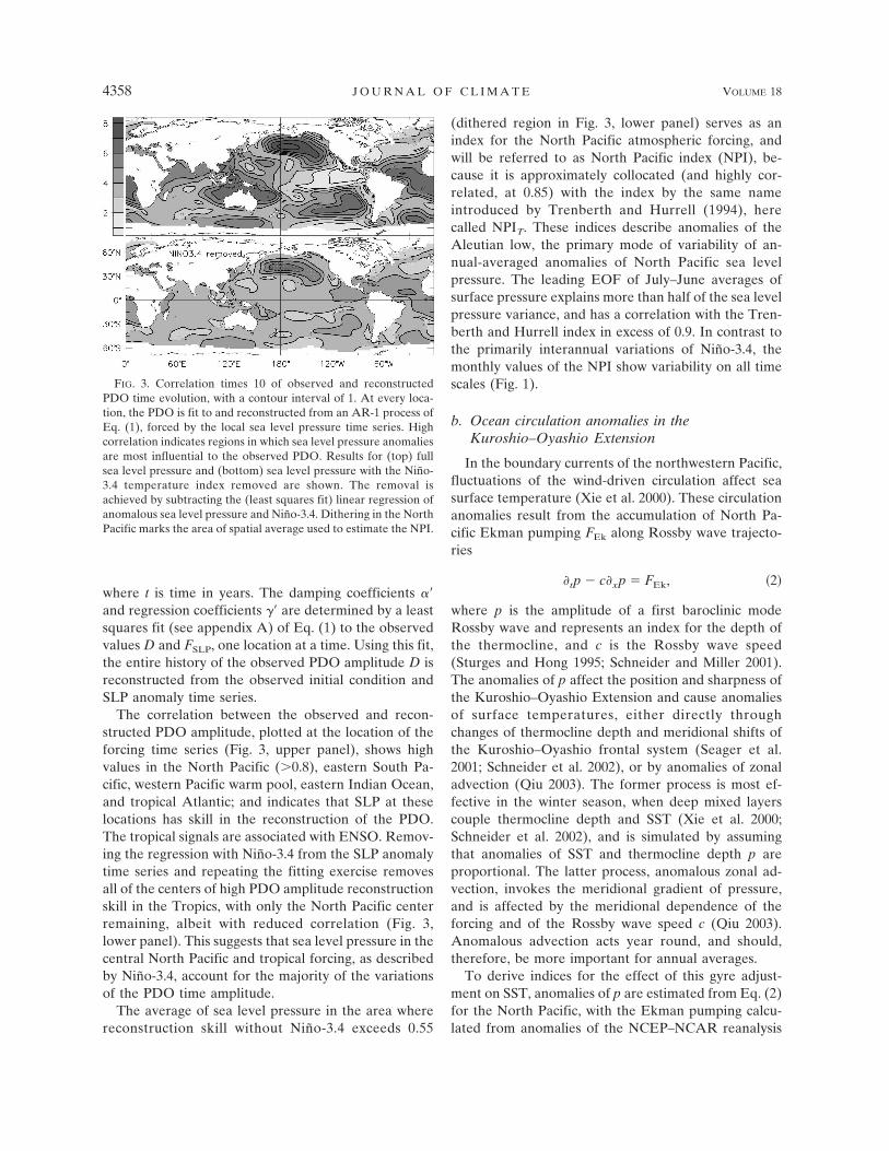
The correlation between the observed and recon-structed PDO amplitude, plotted at the location of theforcing time series (Fig. 3, upper panel), shows highvalues in the North Pacific (0.8), eastern South Pa-cific, western Pacific warm pool, eastern Indian Ocean,and tropical Atlantic; and indicates that SLP at theselocations has skill in the reconstruction of the PDO.The tropical signals are associated with ENSO. Remov-ing the regression with Niño-3.4 from the SLP anomalytime series and repeating the fitting exercise removesall of the centers of high PDO amplitude reconstructionskill in the Tropics, with only the North Pacific centerremaining, albeit with reduced correlation (Fig. 3,lower panel). This suggests that sea level pressure in thecentral North Pacific and tropical forcing, as describedby Niño-3.4, account for the majority of the variationsof the PDO time amplitude.

The average of sea level pressure in the area wherereconstruction skill without Niño-3.4 exceeds 0.55

(dithered region in Fig. 3, lower panel) serves as anindex for the North Pacific atmospheric forcing, andwill be referred to as North Pacific index (NPI), be-cause it is approximately collocated (and highly cor-related, at 0.85) with the index by the same nameintroduced by Trenberth and Hurrell (1994), herecalled NPIT. These indices describe anomalies of theAleutian low, the primary mode of variability of an-nual-averaged anomalies of North Pacific sea levelpressure. The leading EOF of July–June averages ofsurface pressure explains more than half of the sea levelpressure variance, and has a correlation with the Tren-berth and Hurrell index in excess of 0.9. In contrast tothe primarily interannual variations of Niño-3.4, themonthly values of the NPI show variability on all timescales (Fig. 1).

b. Ocean circulation anomalies in theKuroshio–Oyashio Extension

In the boundary currents of the northwestern Pacific,fluctuations of the wind-driven circulation affect seasurface temperature (Xie et al. 2000). These circulationanomalies result from the accumulation of North Pa-cific Ekman pumping FEk along Rossby wave trajecto-ries

�tp � c�xp � FEk, �2�

where p is the amplitude of a first baroclinic modeRossby wave and represents an index for the depth ofthe thermocline, and c is the Rossby wave speed(Sturges and Hong 1995; Schneider and Miller 2001).The anomalies of p affect the position and sharpness ofthe Kuroshio–Oyashio Extension and cause anomaliesof surface temperatures, either directly throughchanges of thermocline depth and meridional shifts ofthe Kuroshio–Oyashio frontal system (Seager et al.2001; Schneider et al. 2002), or by anomalies of zonaladvection (Qiu 2003). The former process is most ef-fective in the winter season, when deep mixed layerscouple thermocline depth and SST (Xie et al. 2000;Schneider et al. 2002), and is simulated by assumingthat anomalies of SST and thermocline depth p areproportional. The latter process, anomalous zonal ad-vection, invokes the meridional gradient of pressure,and is affected by the meridional dependence of theforcing and of the Rossby wave speed c (Qiu 2003).Anomalous advection acts year round, and should,therefore, be more important for annual averages.

To derive indices for the effect of this gyre adjust-ment on SST, anomalies of p are estimated from Eq. (2)for the North Pacific, with the Ekman pumping calcu-lated from anomalies of the NCEP–NCAR reanalysis

FIG. 3. Correlation times 10 of observed and reconstructedPDO time evolution, with a contour interval of 1. At every loca-tion, the PDO is fit to and reconstructed from an AR-1 process ofEq. (1), forced by the local sea level pressure time series. Highcorrelation indicates regions in which sea level pressure anomaliesare most influential to the observed PDO. Results for (top) fullsea level pressure and (bottom) sea level pressure with the Niño-3.4 temperature index removed are shown. The removal isachieved by subtracting the (least squares fit) linear regression ofanomalous sea level pressure and Niño-3.4. Dithering in the NorthPacific marks the area of spatial average used to estimate the NPI.


wind stress (Schneider and Miller 2001). The Rossbywave speeds are based on satellite observations of sealevel (Qiu 2003). The estimates p are averaged in theKuroshio–Oyashio Extension between 140° and 170°E,and a thermocline depth index PAVG is then obtainedby the average between 35° and 40°N; the zonal advec-tion index PDEL is evaluated by differencing the zonal-averaged p between 38° and 40°N. The latitudes corre-spond to the location of the Kuroshio–Oyashio Exten-sion region and were refined by trial and error, aselection procedure that is considered in the estimationof the significance (see below).

The Kuroshio–Oyashio Extension thermocline depthindex PAVG and zonal advection index PDEL are domi-nated by variance at decadal frequencies (Fig. 1), asexpected from the integration of atmospheric forcingalong Rossby wave trajectories (Frankignoul et al.1997), and can only account for a significant fractionof SSTA at long time scales. The KOE indices arelargely independent of wind stress curl anomalies thatare associated with Niño-3.4 and NPI. Removal of theregression of the wind stress curl with these indicesbefore the solution of Eq. (2) has very little impact onPDEL and merely removes a trend from PAVG (dottedlines in Fig. 1).

4. Reconstruction of SST

The PDO is defined as the leading mode of SSTA, sowe begin by reconstructing SSTA, and will later returnto examine how well the leading EOF of the recon-structed SSTA compares to the actual PDO.

a. Approach

The budget for surface temperature anomalies T isassumed to be governed by an AR-1 model (Hassel-mann 1976)

�tT�x, y, t� � ��x, y�T�x, y, t� � �i�x, y�Fi�t�, �3�

where t is time; � is the damping rate; and the differ-ent forcing terms, denoted by index i, have the timeevolution Fi with a spatial footprint i; and a repeatedindex i implies the Einstein summation convention.The first term on the right-hand side represents thedamping of SST anomalies by the air–sea heat fluxes,with a decay rate � determined by the feedback of theair–sea heat flux and by the mixed-layer depth. Whilethese processes and thus � have a seasonal cycle, wefocus on the time scales that are longer than a year, sothat � is taken as a constant representative value for theentire year. Considering heat content from the surfaceto winter mixed-layer depths would remove the

complications that are associated with the seasonalcycle of the mixed layer and the reemergence of tem-perature anomalies (Deser et al. 2003). However, thePDO is defined with respect to SST, and we need todetermine the relationship between seasonal variationsresulting from reemergence and the representative an-nual value � of the feedback. In appendix B, an exten-sion of the Hasselmann (1976) model to include re-emergence is used to show that the � derived fromannual averages of SST lies between summer and win-ter damping rates, but close to winter values.

Equation (3) is discretized to describe the year-to-year evolution of July–June averages of temperatureanomalies. With � constant in time, Eq. (3) is integratedover 1 yr, and then averaged from July to the subse-quent June. This yields for the annual-averaged valueof temperature anomalies at every location x, y

T�x, y, t� � �i�x, y��t��

t

dt�Fi�t��e��x,y��t�t��

� e��x,y��T�x, y, t � ��, �4�

�: �i�x, y� Fi�x, y, t� � ��x, y�T�x, y, t � ��,

�5�

where � is the 1-yr time step of the discretization, andthe overline represents July–June 12-month averages.The annual-averaged value of SSTA results from itsvalue of the previous year, discounted at a rate of �,and the annual averages of the forcing fields, whichhave been filtered by a one-sided exponential with de-cay � resulting from the damping of temperatureanomalies. For ease of reference, Fi is defined in Eq. (5)as the annual average of the filtered forcing time serieswith filter coefficients varying in x, y, and � �exp(��) is the discretized autoregressive parameter.

The discretized temperature in Eq. (4) preserves thelead–lag relationships of Eq. (3) between the forcingand temperature, unlike the ad hoc approach of Eq. (1),which relates the value of the PDO to contemporane-ous forcing fields. A slight complication arises from thespatial dependence of � that renders the filtered forcingfunction Fi as a function of time and space, and pro-duces nonseparable forcing for the evolution of annu-ally averaged temperature anomalies. However, we willfind that � has only a weak spatial dependence so thatthe spatial variance of forcing functions Fi are small andnot important.

The reconstruction of North Pacific SST anomaliesreduces to an exercise of fitting the observed evo-lution of T(x, y, t) to the right-hand side of Eq. (4) byadjusting the damping �(x, y) and spatial footprints of


the forcing i(x, y) at every location. Equation (4) isnonlinear in � as a result of the filtering of the forcingtime series, and the coefficients are determined itera-tively. Starting from a first guess of �, the time integralsof Fi and June–July averages are formed to yield Fi. Wethen determine � and i from Eq. (5) by multilinearregression using a least squares approach (see appendixA), and repeat the procedure with the new estimate of� obtained from �. Typically, this procedure convergesin less than 10 iterations.

The skill of the fit is determined by comparison of theobserved and fitted temperatures, and is obtained intwo related ways: as a 1-yr “forecast” of year n from theobserved previous year’s SSTA and the forcing timeseries2 (the procedure followed by Newman et al. 2003when comparing the observed and fitted time evolutionof the PDO), or from a 50-yr “hindcast,” initializing Eq.(5) with the observed 1950/51 July average and deter-mining the evolution until 2002/03 using only the forc-ing time series. The two approaches yield essentiallythe same results, albeit with the hindcast—the moredemanding test—exhibiting overall lower skill valuesthan that of the forecast, and we will present the hind-cast skills only.

The significance of the reconstruction and of eachregression pattern is estimated by comparison to theperformance of the null hypothesis: that a selection ofrandom red-noise series can do as well as the physicallymeaningful series chosen here. Figure 4 shows the 95%highest correlation level from 1000 reconstructions ofthe annual-averaged values of the PDO from the red-noise time series that have the same 1-yr lag autocor-relation as the annual averages of the index series Fi. Toaccount for artificial skill, we repeat with the noise timeseries the “prospecting” used in choosing the NPI,PAVG, and PDEL by assuming that the NPI was selectedout of North Pacific sea level pressure from 20 inde-pendent regions or modes, and that the PDEL and PAVG

were selected each from a total of five possible latitudebands. These estimates of the degrees of freedom aredeliberately high, so as to yield a conservative estimateof significance.

Specifically, each reconstruction of the PDO fromthe noise time series is obtained just as in the analysis ofthe observations. The observed PDO is fit to an AR-1process that is forced by one “NINO3.4” noise realiza-tion. The residual is then reconstructed using 20 inde-pendent “NPI” noise time series, and the realizationwith the best fit is chosen. We then choose the best of

five noise realizations each for PDEL and PAVG thatcapture the SSTA variations of a representative timeseries in the western North Pacific. For this set of “best”noise forcings, we obtain the PDO reconstruction skill,and then determine at every point in the North Pacificthe combined skill of the noise series in the reconstruc-tion of observed SSTA and the individual skill of eachof the forcing indices.

For the PDO reconstruction, this yields 95% (90%)significance levels of the hindcast correlation of 0.68(0.66). The 95% significance levels of the SSTA recon-struction skill (Fig. 4) reach values of 0.6–0.65 in thecentral and eastern North Pacific, and mimic the horse-

2 Note that this is not strictly a prediction because the values ofthe forcing time series are assumed to be known up to time n.

FIG. 4. (top) The significance levels (95%) of the correlation of50-yr hindcast of observed SSTA and best-fit AR-1 model forcedby red-noise time series. (bottom four panels) The 95% signifi-cance levels for the contributions of Niño-3.4, NPI, PDEL, andPAVG, respectively. The significance levels are based on 1000 re-constructions of SSTA, and include the effect of artificial skillfrom the selection used in deriving some of the forcing indices.Contour interval is 0.1.


shoe pattern of the PDO. The 95% significance levelsof the individual forcing indices vary by about 0.4 forNiño-3.4, and between 0.45 and 0.55 for NPI, PDEL, andPAVG.

b. Skill

The reconstruction of SSTA based on the forcingindices of ENSO, NPI, PDEL, and PAVG is very success-ful in the North Pacific. Correlations of the hindcastand observations of SSTA (Fig. 5) are larger than 0.75in the areas of large loading of the PDO in the centraland eastern North Pacific (Fig. 2, top) and mimicclosely the variance of SSTA that is explained by thePDO itself. The skill in these regions is significant because it exceeds the 95% significance levels that are

derived above (Fig. 4). The reconstruction passes thesignificance test except south of 25°N, and along thezero line of the PDO pattern.

Central to our purpose here is the comparison of theleading EOF of observed SSTA and its reconstructionfrom the hindcast. The spatial patterns of original andreconstructed fields are nearly identical (Fig. 2), with apattern correlation in excess of 0.9 (Table 1). Smalldifferences occur in the amplitudes of the spatial pat-tern in the central North Pacific, where the ridge of highloading extends further east in the reconstruction. Theprincipal component also shows a good fit (Fig. 6), withall transitions captured. The correlation of observedand reconstructed PDO is 0.93, which is highly signifi-cant (Table 1). The only differences occur in slightlyreduced amplitudes in the late 1950s and 1990. Thissuggests that the processes underlying the PDO arecaptured, and the reconstruction can be used to explorethe properties of the PDO.

The hindcast skill of the individual components (Fig.5) shows that Niño-3.4, NPI, and PDEL account for sig-nificant fractions of North Pacific SSTA variability. Theskill of Niño-3.4 is largest in the eastern portion of thebasin and along the coast of North America, while NPIaccounts for the largest variations along 40°N and in thecentral and the western portion of the Pacific. Thezonal advection index has skill in the Kuroshio–Oyashio Extension, as expected. The contribution ofPAVG, while revealing a physically plausible pattern (aswill be discussed below), nowhere exceeds the skill thatis expected from an arbitrary red-noise process, andPAVG will therefore not be considered in the recon-struction of the PDO.

c. Damping time scale

The lag-1 autocorrelation of annual averages ofSSTA � is largely a constant in space with typical values

TABLE 1. Correlation coefficients of observed PDO (top) pat-terns and (bottom) principal component with leading EOF of theSSTA reconstruction using spatially varying � (column 1) or con-stant �0 (column 2). Column 3 shows the results obtained fromsetting the off-diagonal elements of the covariance matrix of theforcing indices to zero, and column 4 shows results from consid-ering only the forcing by Niño-3.4* and NPI*.

�(x) �0

�0, notemporal

covariance

�0,Niño-3.4*,NPI* only

Pattern 0.98 0.98 0.98 0.98Principal component 0.93 0.93 0.93 0.89

FIG. 5. (top) Correlation times 10 of 50-yr AR-1 model SSTAhindcast and observed Jul–Jun averages of SSTA. (bottom fourpanels) Correlation of observed and hindcast SSTA using onlyforcing by Niño-3.4, NPI, PDEL, and PAVG, respectively. Contourinterval is 2.


of 0.2–0.3, and corresponds to a damping time scale ��1

of 7.5–10 months (Fig. 7). Off the coasts of Japan andChina the damping times are larger, but in these areasskill is small, and not significant (Figs. 4, 5). The damp-ing time reflects the feedback � to surface temperature

of the air–sea heat flux, normalized by an effectivemixed-layer depth H, and the density 0 and heat ca-pacity cp of seawater. With � � 15 W m�2 K�1 (Deseret al. 2003), 0 � 1000 kg m�3 and cp � 4 · 103 J kg�1

K�1, the effective annually averaged mixed-layer depthis H � �( 0cp�)�1, and varies between 74 and 98 m. Thisis shallower than the deep wintertime mixed-layerdepths that are required to explain the autocorrelationof the upper-ocean heat content (Deser et al. 2003), butis consistent with our focus on annually averaged seasurface temperature anomalies and typical mixed-layerdepths of the North Pacific (see appendix B).

d. Forcing time series

Given the damping time scales, the filtered forcingtime series Fi can be obtained and are shown in Fig. 6,normalized to unit standard deviation. The filteredNiño-3.4 series shows the major El Niño and La Niñaevents, slightly delayed, as expected, from the integra-tion. The 1976/77 change is marked by several years ofdepressed Niño-3.4, followed after the shift by a recov-ery to near-normal forcing. The NPI time series dis-plays more year-to-year variability and also shows atrend to more negative values, punctuated by dramaticvariations of either sign. The transition to higher valuesafter 1986 corresponds to an intensified Pacific stormtrack that is reported by Nakamura et al. (2002, theirFig. 5).

The spatial dependence of each Fi is shown in Fig. 6by its spatial average (thin black line) and its standarddeviation (vertical bars). As expected from the smallvariability of �, the scatter of Fi is small, so small, infact, that the standard deviation is only perceptible forNPI, which has the largest variance at high frequenciesand is therefore most sensitive. The pressure (KOE)indices are hardly changed from their unfiltered Fi, be-cause their variance is dominated by interannual anddecadal time scales, and are not affected by the filteringoperation. Thus, our calculations and the forcing foot-prints i are insensitive to the exact values of � in thefiltering of the monthly forcing indices Fi to the annualaverages Fi, and much the same results are obtained byfiltering the forcing functions with a constant value of��1 of 3/4 yr.

e. Orthogonalization matrix

The forcing time series Fi are not independent, andwe have to account for their shared variance. While theindependent components of each Fi are sufficient todetermine their unique regression patterns their corre-lated components imply that any particular forcing has

FIG. 7. Estimate of damping time ��1 of Eq. (3) in months.Contour interval is 10 months.

FIG. 6. (top) Time series of Jul–Jun annual averages of PDO(black line). Overlaid in gray is the PDO based on SSTA recon-struction. (bottom four) The Fi(t) for Niño-3.4, NPI, PDEL, andPAVG, respectively, are shown. Thin solid lines denote the spatialaverages of the filtered index time series, and tiny vertical barstheir spatial standard deviation. Dashed lines show the rotatedtime series Fi(t)*, and the thick gray lines denote their projectiononto the observed pattern of the PDO [see Eq. (7)]. All timeseries have been normalized to unit standard deviation.


an indirect impact on SSTA through the other timeseries. To quantify these relationships, we determinethe rotation matrix Bij that relates Fi to an orthogonalbase F*j ,

�iFi�t� � �iBijF*j �t�, �6�

with rotated regression pattern *j � iBij. The matrixBij is obtained from a Gram–Schmidt orthogonalizationthat leaves the Niño-3.4 time series unchanged, re-moves from NPI the regression with Niño-3.4, removesfrom PDEL the multilinear regression with Niño-3.4 andNPI, and so on. This order reflects the hypothesis thatanomalies of the Aleutian low pressure, the NPI, resultin part from teleconnections from the Tropics (i.e.,Niño-3.4) and that anomalies in the Kuroshio–OyashioExtension are in part a response to forcing of ENSOand the NPI.

The rotation matrix Bij (Table 2) is estimated withboth Fi and F*j normalized to unit variance, so that thesquare of any element Bij represents the variance of Fi

captured by the F*j . Only the following two nontrivalrelationships emerge: Niño-3.4 is negatively correlatedwith NPI and accounts for 30% of its variance, andPDEL is weakly related to PAVG and accounts for 6% ofits variance; all of the remaining elements are small.Thus, the rotated F*j , shown in Fig. 6 as dashed lines,only differ from Fi for NPI and PAVG.

Note that the Gram–Schmidt orthogonalizationcould start with NPI and attribute the covariance ofNPI and Niño-3.4 to changes of the NPI. Physically,this suggests that the extratropics modulate ENSO viateleconnections to the Tropics (Barnett et al. 1999a;Pierce et al. 2000) or provide stochastic forcing forENSO (Vimont et al. 2001, 2003). However, it seemsunlikely that ENSO variability is completely deter-

mined by the NPI, and so we do not treat this option indetail, although it is statistically appealing.

f. Forcing footprints

The forcing terms i(x, y) Fi(x, y, t) in Eq. (5) repre-sent the annually averaged SSTA that is the result ofthe forcing i after 1 yr. Results are shown for Fi(x, y, t)normalized to unit standard deviation at every location,so that the maps of the regression coefficients i(x, y)show the pattern of SSTA caused by a typical ampli-tude of the filtered forcing time series Fi. Overall, thepatterns are consistent with underlying physical pro-cesses and the results from prior studies.

The NPI regression pattern dominates the regression(Fig. 8, bottom), with large amplitudes over the westernNorth Pacific and the Kuroshio–Oyashio frontal re-gions, surrounded by anomalies of the opposite sign inthe eastern Pacific and in the Gulf of Alaska. A highsea level pressure perturbation of the Aleutian low isassociated with increased temperatures in the centralNorth Pacific along 40°N, and cooler temperatures inthe eastern Pacific, the Gulf of Alaska, and the subpo-lar region (Davis 1976). These changes are associatedwith anomalies of the Pacific storm track (Nakamura etal. 2002; An and Wang 2005), and are consistent with adecrease of westerlies that reduces turbulent heat lossesand causes poleward Ekman advection in the centralNorth Pacific. Cooling tendencies in the east are con-sistent with advection of cold and dry air from the highlatitudes (Tanimoto et al. 2003).

TABLE 2. Rotation matrix Bij that converts the orthogonal forc-ing time series F*j , denoted by top row to the forcing time seriesFi, denoted by the leftmost column. The original and rotated timeseries are all normalized to unit standard deviations, so that thevariance explained by F*j is given by the square of the values ofthe table. The values are the spatial mean of the rotation matrixat every location; however, the spatial variations are very small,and the standard deviation of the nonzero elements are of theorder of 0.001 or smaller.

Niño-3.4* NPI* P*DEL P*AVG

Niño-3.4 1 0 0 0NPI �0.55 0.83 0 0PDEL 0.10 0.07 0.99 0PAVG �0.07 �0.03 0.24 0.97

FIG. 8. Forcing footprints i(x, y) of (top) Niño-3.4 and (bot-tom) NPI. The maps represent the response of SST (K) after theforcing of unit magnitude has been applied for 1 yr. Contourinterval is 0.1, and negative contours are dotted.


The pattern associated with Niño-3.4 (Fig. 8, top) hasthe most loading in the eastern Pacific and along thecoast of North America, with opposite-signed anoma-lies farther offshore. This pattern captures coastal waveprocesses and atmospheric teleconnections that are in-dependent of the NPI, and, as we will show below,together with the correlated contribution of the NPI,forms the well-known SST response pattern to tropicalvariations.

The zonal advection index in the northwestern Pa-cific (PDEL) is associated with temperature anomaliesin the Kuroshio–Oyashio Extension (Fig. 9, top), andoverlaps with the regions of influence of the Niño-3.4and NPI. A positive index, corresponding to an increaseof eastward flow, leads to warming centered west of thedate line, spreading along 40°N. The warming is shiftedto the east-northeast of the region of the ocean pressureindex (indicated by dotted lines in Fig. 9), consistentwith downstream advection by the mean flow, whichhas a east-northeasterly direction in the Kuroshio–Oyashio Extension (Qiu 2003).

The thermocline depth index (PAVG) in the Kuro-shio–Oyashio Extension shows little effect on annual-averaged SSTA (Fig. 9, bottom). Yet, the dipole pat-tern of warm anomalies at 42°N and cool anomalies at35°N in response to a positive anomaly of PAVG is con-sistent with a northward shift of the Kuroshio–OyashioExtension axis. The weak signal is consistent with the

annual cycle of mixed-layer depth, which links ther-mocline depth and surface temperature only during thewintertime, when mixed layers are deep (Schneider andMiller 2001). For annual averages, this process accountsfor only a small fraction of the variance.

g. Rotated forcing footprints

According to Eq. (6), the rotated forcing footprint *of Niño-3.4* augments the unrotated ENSO footprintwith the unrotated pattern of NPI, PDEL, and PAVG,with weights Bij given by the first column of Table 2.The resulting Niño-3.4* pattern (Fig. 10, top) extendsthe unrotated Niño-3.4 pattern (Fig. 8, top) to the west,primarily by the addition of the unrotated NPI patterns(Fig. 8, bottom). It is the canonical response of theNorth Pacific SST to ENSO and corresponds to thecomposite ENSO response of the North Pacific to theensemble-averaged response obtained from models,and to the pattern removed from North Pacific SSTAby regression with an index for the cold tongue SSTA(Zhang et al. 1997).

The rotated * of Niño-3.4* captures the annuallyaveraged footprint resulting from the atmosphericbridge (Alexander et al. 2002, 2004) between ENSO(Niño-3.4) and the Aleutian low (NPI) and the atmo-sphere of the eastern North Pacific, and resulting fromthe oceanic connection by coastal wave propagation offof North America equatorward of 40°N (Chelton andDavis 1982; Clarke and Lebedev 1999; Lluch-Cota et al.

FIG. 9. Regression pattern with Kuroshio–Oyashio Extensioncirculation indices of (top) zonal advection and (bottom) ther-mocline depth. Units are in kelvins and correspond to the re-sponse of SST after the forcing of unit magnitude has been ap-plied for 1 yr. Contour interval is 0.1, negative contours are dot-ted, and the zero contour is omitted. Thin dashed lines indicatethe areas used in the calculation of the indices.

FIG. 10. Rotated footprints for i(x, y)* of (top) Niño-3.4* and(bottom) NPI*. The maps represent the response of SST (K) afterthe forcing of unit magnitude has been applied for 1 yr. Contourinterval is 0.1, and negative contours are dotted.


2001). Overall, El Niño is associated with low tempera-tures in the central North Pacific in boreal fall and win-ter, and along the Kuroshio–Oyashio Extension in bo-real summer (Alexander et al. 2004), and with warmanomalies in the eastern Pacific and in the Gulf ofAlaska. Alexander et al. (2002) attribute the anomaliesof SST to changes of the surface heat flux, entrainment,and Ekman advection, together of the order of 20 Wm�2 in the cooling region east of the date line. Similarnumbers are obtained from ship observations (Tan-imoto et al. 2003). To compare this heat flux with themagnitude of the regression pattern of 0.2–0.3 K, weinterpret the F time series of Niño-3.4 (Fig. 1) as a heatflux time series, with anomalies during ENSO of 20 Wm�2 that are typical during ENSO events and equiva-lent to the two standard deviations. Applying this heatflux to a layer of 80-m depth, and estimating the cor-responding F time series via the definition implied byEq. (5), yields a standard deviation of annual-averagedvalues of SSTA of 0.4 K, which are roughly consistentwith Fig. 10 (top).

The rotated NPI* pattern is almost identical to itsunrotated counterpart, because the contributions fromPDEL and PAVG are small (second column of Table 2).The * associated with NPI* indicates that anomalies at40°N (Fig. 10, bottom) are consistent with decadal win-tertime temperature anomalies independent of ENSO,resulting from shifts of the North Pacific subarcticfronts (Nakamura et al. 1997; Nakamura and Yamagata1999; Nakamura and Kazmin 2003).

The rotated pattern of PDEL (not shown) is enhancedslightly between 40° and 45°N west of the date linebecause of the contribution from PAVG (Table 2, thirdcolumn). Applying instead the variance that is sharedbetween the two KOE indices to PAVG enhances itsnorthern loading. However, this increase is not suffi-cient to raise the variance that is associated with PAVG

beyond the significance level.

5. PDO properties

a. Kinematics

Using the autoregressive model for SSTA and theregression patterns, we now investigate the evolutionequation for the PDO. The equation governing thetime evolution of the PDO is derived by projecting Eq.(5) on the leading empirical orthogonal function of an-nual-averaged values of temperature anomalies

a0�t� � ��0�k�ak�t � 1� � ��i�0Fi�, �7�

where ak is the principal component and �k the or-thonormal spatial loading pattern of mode k, with thePDO being k � 0, and � � denoting the spatial projec-tion. In general, the spatial dependence of � couples theevolution of the PDO and the other principal compo-nents. The forcing of the PDO amplitude, the last termon the right-hand side of Eq. (7), can be written foreach i as the product of the regression coefficient �i�0�and the weighted spatial average of the forcing timeseries �i�0�

�1 �i�0Fi�. Because the spatial depen-dence of Fi is weak, the weighting has little effect, andthe forcing time series for the PDO are indistinguish-able from the spatial means of Fi(x, y, t) (cf. black andgray lines in Fig. 6).

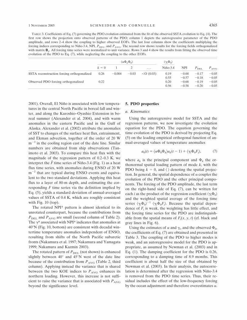
Using the estimates of � and i, and the observed �0,the coefficients of Eq. (7) are obtained and presented inTable 3. The coupling of the PDO to higher modes isweak, and an autoregressive model for the PDO is ap-propriate, as assumed by Newman et al. (2003) and inEq. (1). The damping coefficient for the PDO is 0.26,corresponding to a damping time of 8.9 months. Thiscoefficient is about half the size of that obtained byNewman et al. (2003). In their analysis, the autocorre-lation is determined after the regression with Niño-3.4is removed from the PDO time series. Thus, their re-sidual includes the effect of the low-frequency forcingby the ocean adjustment and therefore overestimates �.

TABLE 3. Coefficients of Eq. (7) governing the PDO evolution estimated from the fit of the observed SSTA evolution to Eq. (4). Thefirst row shows the projection onto observed patterns of the PDO; column 1 depicts the autoregressive parameter of the PDOamplitude, and rows 2–4 show the coupling to higher observed EOFs. The last four columns show the coefficients multiplying theforcing indices corresponding to Niño-3.4, NPI, PDEL, and PAVG. The second row shows results for the forcing fields orthogonalizedwith matrix Bij. All forcing time series were normalized to unit variance. Rows 3 and 4 show the results from fitting the observed timeevolution of the PDO to Eq. (7), while neglecting the coupling to the other EOFs.

��k�0� �i�0�

k � 0 1 2 . . . Niño-3.4 NPI PDEL PAVG

SSTA reconstruction forcing orthogonalized 0.26 �0.004 �0.03 �O (0.03) 0.19 �0.68 �0.17 �0.050.55 �0.57 �0.18 �0.05

Observed PDO forcing orthogonalized 0.22 0.20 �0.68 �0.19 �0.050.56 �0.58 �0.20 �0.05


The weights of the forcing fields that are projectedonto the PDO are determined with Fi normalized tounit standard deviation, and are shown as gray lines inFig. 6. The forcing functions are indistinguishable fromthe individual Fi and their spatial means, showing theweak variations imparted by the spatial dependence of�. While the forcing by NPI clearly dominates, a sig-nificant fraction of the NPI response results from tele-connections with Niño-3.4. The orthogonalization toNiño-3.4* and NPI* yields about equal weights forthese forcings, with opposite signs. Thus, ENSO pri-marily affects the PDO via changes of the Aleutian low(and NPI), and leads to the known relationships be-tween ENSO and the PDO—warm conditions in theeastern equatorial Pacific are associated with a coolcentral North Pacific and a warm eastern North Pacific.Positive values of the NPI* indicate a reduced Aleutianlow, with warmer temperatures in the central NorthPacific (and, thus, negative anomalies of the PDO). Thezonal advection index PDEL in the Kuroshio–OyashioExtension has about one-third of the weight comparedto the NPI*, and indicates that increased advectionleads to warm conditions and negative values of thePDO.

As a consistency test, we fit the observed evolution ofthe PDO amplitude to Eq. (7), while neglecting thecoupling to higher EOFs of SSTA. This yields a slightlyreduced damping coefficient, and very similar coeffi-cients of the forcings (Table 3, bottom two rows).

In the following, we will restrict the discussion to therotated forcing fields and regression pattern, notingthat a significant fraction of the ENSO forcing affectsNorth Pacific SSTA and the PDO via the NPI.

b. PDO evolution

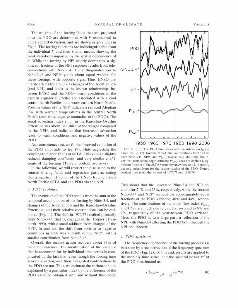
The evolution of the PDO results from the sum of thetemporal accumulation of the forcing by Niño-3.4, andchanges of the Aleutian low and the Kuroshio–OyashioExtension, and their relative contributions can be esti-mated (Fig. 11). The shift in 1976/77 resulted primarilyfrom Niño-3.4*, that is, changes in the Tropics (Tren-berth 1990), with a small addition from changes of theNPI*. In contrast, the shift from positive to negativeconditions in 1998 was a result of the NPI*, with asmaller contribution from Niño-3.4*.

Overall, the reconstruction recovers about 83% ofthe PDO variance. The identification of the variancethat is accounted for by individual time series is com-plicated by the fact that, even though the forcing timeseries are orthogonal, their integrated contributions tothe PDO are not. Thus, we estimate the variance that isexplained by a particular index by the difference of thePDO variance obtained with and without this index.

This shows that the unrotated Niño-3.4 and NPI ac-count for 21% and 73%, respectively, while the rotatedNiño-3.4* and NPI* account for approximately equalfractions of the PDO variance, 40% and 44%, respec-tively. The contributions of the zonal flow index PDEL

and P*DEL are much smaller, and correspond to 6% and7%, respectively of the year-to-year PDO variance.Thus, the PDO is, to a large part, a reflection of theNPI, with Niño-3.4 affecting the PDO both through theNPI and directly.

c. PDO spectrum

The frequency dependence of the forcing processes isbest seen by a reconstruction of the frequency spectrumof the PDO (Fig. 12). To this end, results are applied tothe monthly time series, and the spectral power P2 ofthe PDO is estimated as

PPDO2 �

1

�2 � �02 ��iPi�

2, �8�

FIG. 11. (top) The PDO time series and reconstruction (gray)based on Eq. (7). (middle three) The contributions to the PDOfrom Niño-3.4*, NPI*, and P*DEL, respectively. (bottom) The in-dex for thermocline depth estimate P*AVG does not explain a sig-nificant fraction of the SSTA variability anywhere and is thereforedeemed insignificant for the reconstruction of the PDO. Dottedvertical lines mark the winters of 1976/77 and 1998/99.


where � is the frequency, �0 � ��1 loge(��0�0�), andP2

i are the power spectra of the forcing indices. Thespectrum of the reconstruction has a very good agree-ment with the observed spectrum (Fig. 12), with a slightoverestimation at interannual frequencies, which canalso be gleaned from the comparison of the recon-structed and observed PDO time series (Fig. 11). Atannual and shorter time scales, the reconstructed spec-trum slightly, but systematically, underestimates the ob-served spectrum. This is consistent with reemergence,observed in the PDO time series (Newman et al. 2003),and its impact on the spectrum (appendix B).

The contribution (�2 � �20)�12

i P2i of each of the forc-

ing components i shows that the NPI* contributiondominates the response at annual and higher frequen-cies, because the spectrum of the NPI* itself is primarilywhite, with only a slight reddening tendency expected

from thermodynamic air–sea coupling (Barsugli andBattisti 1998; Blade 1997), and a broad, gentle peak atinterannual time scales, likely the result of teleconnec-tions to the Tropics. The spectrum of Niño-3.4* hasmost power at interannual frequencies, with a stronglow-frequency component. Its contribution to the PDOincreases rapidly, approximately as ��4, toward inter-annual frequencies, and then decreases slightly towarddecadal time scales. The spectrum of the zonal advec-tion index P*DEL is red with all of its power at lower-than-interannual frequencies, and P*DEL adds to thepower of the PDO only at decadal time scales. There,however, its contribution to the PDO is on par with theNPI* and Niño-3.4*. Thus, the frequency spectrum ofthe PDO (Fig. 12) reflects the effects of the NPI* atperiods of a year and higher. At interannual frequen-cies, Niño-3.4* and NPI* explain the variability, whileat lower frequencies NPI*, Niño-3.4*, and P*DEL are ofequal importance.

d. Relation of PDO and regression patterns

Because the evolution of SSTA over the North Pa-cific is determined by three different forcing indices andpatterns, so is the PDO. The regression patterns havelarge overlap, and are not orthogonal, and an empiricalorthogonal function expansion cannot separate theseinto distinct modes. In fact, we hypothesize that thePDO and the relative roles of its individual forcings aredetermined primarily by the spatial covariance of theforcing footprints, even if the time evolution of the forc-ing indices are independent.

To test this hypothesis, we note that the solution toEq. (4) is separable if � is a constant. This approxima-tion is consistent with the lack of coupling of the PDOwith higher modes. A reconstruction of SSTA for �replaced at all locations with �0 � ��0�0� results inalmost identical estimates of the PDO (Fig. 2), with apattern correlation of 0.98 and a temporal correlationof 0.93 with the observed PDO (Table 1).

The solution for the annual-averaged temperatureanomaly at every location and time step t � n� is ob-tained by integration of Eq. (5),

T�x, y, t � n�� *i �x, y��j�1

n

�0n�jF*i �t � j��

�: �*i �x, y�f*i �t � n��, �9�

and is the sum of separable products of the forcingfootprints i and the time integrals fi of the AR-1 solu-tion to each forcing index. The initial values fi are ob-tained from a multilinear fit of SSTA to the i patternsat the initial time n � 0.

FIG. 12. Power spectrum as a function of frequency in cycles peryear of the observed and reconstructed PDO, and its contribu-tions (�2 � �2

0)�12i P2

i resulting from NPI*, Niño34*, and P*DEL

(as indicated). The solid black line denotes the spectrum of theobserved PDO, the light gray line with black center that of thereconstruction. Spectra have been smoothed by three successiveapplications of a five-point running mean. Fluctuations of thespectra for frequencies above 0.6 cpy are not significant.


The covariance matrix R of temperature anomalies,whose leading eigenvector is the PDO, is then

R � T T� � �*f*�f*�*�, �10�

where T, �*, and f* are written in matrix notation, withprime denoting the transpose. The matrix R is con-structed from the covariance of the regression fields �*,weighted by the covariance (correlation) of f. The latteris dominated by the diagonal elements. To test whetherthe spatial pattern of the PDO is determined by thecovariance of � even if the forcing indices are indepen-dent, a test covariance matrix R is made using Eq. (10)by setting off-diagonal elements of f�f to zero. Again,the PDO pattern from this test matrix is almost identi-cal to the observed pattern, with spatial and temporalcorrelations with observations of 0.98 and 0.93, respec-tively (Table 1), suggesting that the pattern of the PDOand the weights of the separate forcings result from thenonorthogonality of the forcing footprints. In fact, thepattern of the PDO can be recovered by consideringonly Niño-3.4* and NPI* in the estimation of R (Table1, rightmost column) with a reduction of the skill of theprincipal component reconstruction commensuratewith the lack of the contribution of PDEL.

e. Robustness of PDO reconstruction

Deser et al. (2004) report that the relationship be-tween winter values of Trenberth and Hurrell’s (1994)NPIT and Niño-3.4, or the CTI (defined as SSTA in6°S–6°N, 180°–90°W, with the global mean SSTA sub-tracted) was weaker in the first half of the twentiethcentury than in the second half. However, the OTI—the leading EOF of a number of indices for westernPacific and eastern Indian Ocean SSTA, anomalies ofcloudiness and rainfall close to the South Pacific con-vergence zone, anomalies of stratus clouds in the east-ern tropical Pacific, and sea level pressure in the tropi-cal Pacific and Indian Oceans—shows consistent varia-tions with the NPI throughout the twentieth century.

For the PDO, the question arises if its reconstructionis sensitive to the choice of the tropical index, and if therelationship between PDO and its forcing is robust inthe earlier part of the twentieth century. To this end,1900–97 time series of the observed PDO, NPIT, andCTI or OTI are fitted to Eq. (4). Indices for the KOEcannot be extended into the earlier half of the centurybecause the wind stress estimates are not available, andforcing of Eq. (2) by a reconstruction of the Pacificwind stress from regressions with Niño-3.4 and NPIfails to recover the KOE indices (see section 3b).

The relationship of the PDO to the tropical indices

alone is sensitive to the choice of the latter. Fitting theobserved evolution of the PDO to the CTI only (New-man et al. 2003) leads a hindcast correlation of 0.52,while the fit of PDO to OTI captures more of the vari-ance with a hindcast correlation of 0.65. However,when Eq. (4) is forced by NPIT and either CTI or OTI,the hindcast skills for the time period 1900–97 are 0.74and 0.68, respectively. Thus, the variance of the NPIT

that can be attributed to tropical forcing is sensitive tothe tropical index, but the tropical indices do not addany information to the reconstruction of the PDO oncethe NPIT (or NPI) is provided. The evolution of thePDO is largely determined by the NPI (Davis 1976),while the changes of the NPI are attributed, in part, toteleconnections from the Tropics (Deser et al. 2004).However, please note that this does not imply thatchanges of the Aleutian low physically account for allchanges of the PDO. Rather, prescription of the NPIcaptures part of the tropical to extratropical telecon-nections through the correlation of NPI and tropicalindices.

The skill of the fit is degraded in the earlier part ofthe twentieth century, compared to the latter, with cor-relations for the period before (after) 1950 being 0.67(0.85) for CTI and 0.61 (0.88) for OTI. Some degrada-tion is expected because all indices are constrained bythe fewer observations in the earlier period.

f. PDO predictability

Using the framework that is presented above, a fore-cast of the PDO requires predictions of NPI, ENSO,and the gyre processes in the Kuroshio–Oyashio Exten-sion. ENSO forecasts have skill at lead times of 1 andpossibly up to 2 yr (Barnston et al. 1999; Chen et al.2004). The ENSO forecasts fix part of the NPI; thecomponent of NPI* resulting from the intrinsic atmo-spheric variability of the Aleutian low is expected tohave very limited predictability, likely less than a year.The predictability of remote forcing from other areas,such as perturbations in the western Pacific or easternIndian Ocean (Deser et al. 2004), remains to be deter-mined. In the Kuroshio–Oyashio Extension, predictiveskill with a lead time of 1–2 yr has been documented forwintertime SSTA by virtue of the Rossby wave propa-gation (Schneider and Miller 2001). The predictabilityof PDEL itself should be better, however, it only ac-counts for a small fraction of the year-to-year variabil-ity of the PDO. Thus, it appears that a forecast of an-nually averaged values of the PDO is possible at a leadtime of up to a few years. This analysis does not indicatemuch hope for a skillful forecast of the PDO at multi-year to decadal time scales.


6. Conclusions

Causes of decadal variability of SSTA in the NorthPacific, and its leading empirical orthogonal function,have long been the subject of intense debate. Here, weshow that the winter-centered, annually averaged val-ues of SSTA and the PDO can be reconstructed withhigh fidelity from an autoregressive model forced byindices that track sea level pressure of the Aleutian low,ENSO, and ocean circulation anomalies in the Kuro-shio–Oyashio Extension region. This implies that NorthPacific SSTA and the PDO are a response to changes ofthe North Pacific atmosphere resulting from its intrinsicvariability, remote forcing by ENSO and other pro-cesses, and ocean wave processes associated withENSO and the adjustment of the North Pacific Oceanby Rossby waves. The relative importance of theseforcing processes for the PDO is frequency dependent:at periods shorter than 1 yr, intrinsic North Pacific vari-ability dominates; at interannual frequencies, changesof the Aleutian low and of ENSO are essential; and atdecadal periods, the ocean circulation anomalies in theKuroshio–Oyashio Extension gain in importance to parwith the other processes.

Under this hypothesis, the PDO is not governed by asingle physical process that defines a climate mode,akin to ENSO, but results from at least three differentprocesses. Of course, correlation is not casuality, andstatistical relations like this one can only be disproved,not proved, but we have presented physical argumentsfor the hypothesized influences and have shown thatrandomly chosen red-noise processes do not approachthe skill of the three indices used here. This hypothesisalso exemplifies the well-known limitation of empiricalorthogonal functions that represent the variance opti-mally, but are not designed to separate multiple forcingfields with nonorthogonal spatial characteristics, as inthe case of the PDO.

These results suggest a model for the origin of thePDO and quantify that both tropical and North Pacificprocesses are at play. The famous 1976/77 shift of thePDO is of tropical origin, as suggested in many previousstudies (e.g., Nitta and Yamada 1989; Trenberth andHurrell 1994; Graham 1994). The symmetry of theSSTA pattern between the northern and southern ex-tratropics is a reflection of the common tropical forcing(Evans et al. 2001).

This study further clarifies the causes of the “impact”of the PDO on climate of the adjacent continental areasand teleconnection patterns from the Tropics. As foundfrom modeling experiments by Pierce (2002), the PDOdoes not excite the climate modulation, but the PDOand these climate anomalies share the same forcing

from the Tropics and from intrinsic variability of theAleutian low. The impact of oceanic anomalies in theKuroshio–Oyashio Extension complicates this pictureat decadal time scales. The atmospheric response tothese anomalies is likely small at best, and we do notexpect a large trace of these in the climate over NorthAmerica (Kushnir et al. 2002; Yulaeva et al. 2001). Fur-thermore, the relative roles of forcing are likely to besite dependent, and our results suggest, therefore, thatthe stratification of climate anomalies or teleconnectionpatterns be based on the underlying indices of ENSOand the NPI, rather than ENSO and the PDO.

A similar conclusion applies to attempts to recon-struct Northern Hemisphere climate from paleodata,such as tree rings (Biondi et al. 2001; Gedalof et al.2002). The atmospheric conditions controlling treegrowth and tree ring properties are a function of thetropical Pacific and NPI, rather than of the PDO. Thus,conditions in the tropical Pacific and the NPI can bereconstructed from an array of tree rings. A reconstruc-tion of the PDO alone will likely miss the impact ofocean circulation anomalies in the Kuroshio–OyashioExtensions, and has to be viewed with caution for dec-adal time scales that correspond to the adjustment timeof the extratropical ocean circulation.

Acknowledgments. The authors thank Drs. Arthur J.Miller, Jim Potemra, Bo Qiu, and Shang-Ping Xie forhelpful discussions, and Drs. Clara Deser, NathanMantua, Hisashi Nakamura, and one anonymous re-viewer for comments on an earlier draft. This researchwas supported by the National Science FoundationGrant OCE00-82543, by the Office of Science (BER),U.S. Department of Energy Grants DE-FG03-01ER63255 and DE-FG02-04ER63862, and by the Na-tional Oceanic and Atmospheric Administration GrantNA17RJ1231. The views expressed herein are those ofthe authors and do not necessarily reflect the views ofNSF, DOE, or NOAA, or any of their subagencies.

APPENDIX A

Least Squares Solution

To find the coefficients of Eqs. (1) and (5) at a point,we rewrite the problem in terms of the unknown pa-rameters z � (�, 1, 2, . . .) and the matrix A withcolumns that are the time series of each index, the tem-perature or PDO amplitude average of year t � �, andthe forcing time series. The vector d is the time series ofobserved temperature or PDO amplitude at year t, andthe residual is r,

d � A · z � r. �A1�


The coefficients z are determined by minimizing thecost function J,

J � �d � A · z�2 � �z�2. �A2�

The norms ||· · ·||2 are chosen as the inverse covariancematrices

J � rT · R�1 · r � �z�T · P�1 · �z�, �A3�

where R is the covariance of the uncertainty in theresiduals r, and P is the covariance of the model pa-rameters z.

Here J is minimized at the point z:

min�J� � �z � z�T · P�1 · �z � z� � constant �A4�

(Liebelt 1967). The inverse of the curvature at the mini-mum is P, and it determines the uncertainty of the so-lution—how much could the solution vary while stilldoing a good job on the objective function.

The solution and uncertainty for the overdeterminedsystem of the application here is obtained by inversionin model space

z � �AT · R�1 · A � P�1��1 · AT · R�1 · d, �A5�

with uncertainty covariance

P � �AT · R�1 · A � P�1��1. �A6�

In this study, we employ a large signal-to-noise ratio,that is, P�1 � 0 and R � I, so that the cost functioninvolves the misfit (residual) variance only. This impliesthat the parameter variance far exceeds that of the re-siduals, and that the elements of z, or the columns of A,

have equal weight. Our solutions are insensitive to anylarge, but finite, choice of signal-to-noise ratio.

APPENDIX B

The Impact of Reemergence

The focus on annual averages filters seasonal pro-cesses. The evolution of SST is particularly affectedby the seasonal cycle of the mixed-layer depth. Tem-perature anomalies formed in deep winter and springmixed layers persist under the seasonal thermoclineduring summer being insulated from the influence ofthe air–sea fluxes. During the erosion of the seasonalthermocline in the subsequent cold season, the deepanomalies are entrained into the mixed layers, and re-emerge at the surface. This reemergence is found in theextratropical SSTA (e.g., Deser et al. 2003) and thePDO time series (Newman et al. 2003), and representsan important departure from the AR-1 hypothesis forSST anomalies. Surface temperature anomalies notonly depend on the anomalies of the prior month, butalso on the anomalies of the previous cold season. Thisinfluences the power of SSTA at biannual to shorter-than-annual time scales (Dommenget and Latif 2002).

To investigate the impact of reemergence on ouranalysis of winter-centered annual averages of SST, weexplore a simple extension of the Hasselmann (1976)model that includes reemergence. Consider a mixedlayer with depth H1 in winter and H2 in summermonths, with a summer seasonal thermocline in thelayer between H1 and H2 (H1 H2). The rate of changeof the surface temperature T is governed by

�tT �Q � �T

0cpH�

H2 � H1

�t

T � Tst

H2�tfall � t � tfall � �t�, �B1�

with H � H1 from fall to spring, and H � H2 fromspring to fall equinox. The air–sea heat flux consists ofa forcing term Q, and feedback component of strength�, normalized by the density of water 0 and its heatcapacity cp. The last term on the right-hand side de-scribes the erosion of the seasonal thermocline and isnonzero only during the entrainment season, whichcommences at the fall equinox tfall and deepens themixed layer to winter values during the period �t. Thisswitch is indicated by the function � that is one only ifits argument is true. The temperature of the seasonalthermocline Tst equals the surface values from the endof the fall entrainment period to spring equinox whenthe seasonal thermocline is nonexistent and absorbed inthe deep winter mixed layer. At the spring equinox at

tspring the mixed layer abruptly shallows to its summerdepth, and the seasonal thermocline becomes insulatedfrom the surface fluxes. Thus, Tst remains at its springvalue throughout the summer until the seasonal ther-mocline is reentrained into the mixed layer in the fall.

This model was implemented with parameters thatare typical for the North Pacific: � � 15 W m2 K�1, 0 �1000 kg m�3, cp � 4000 J kg�1 K�1, H1 � 100 m, tfall �0 months, tspring � 6 months, and Q being Gaussianwhite-noise Q with a standard deviation of 20 W m�2.As the simplest case, we focus on a short entrainmentseason, and choose �t to be zero. In the fall, the mixedlayer instantly deepens to its winter depth. This ideal-ized case recovers the qualitative influence of reemer-gence. More gradual spring shallowing and fall entrain-


ment seasons would simply smooth the autocorrelationfunction shown below. The model was run for 1024 yrfor the same realization of the random Q forcing for areference case, H2 � H1, identical to the Hasselmann(1976) model, and for summertime mixed-layer depthsof H2 � 40 m and of H2 � 20 m.

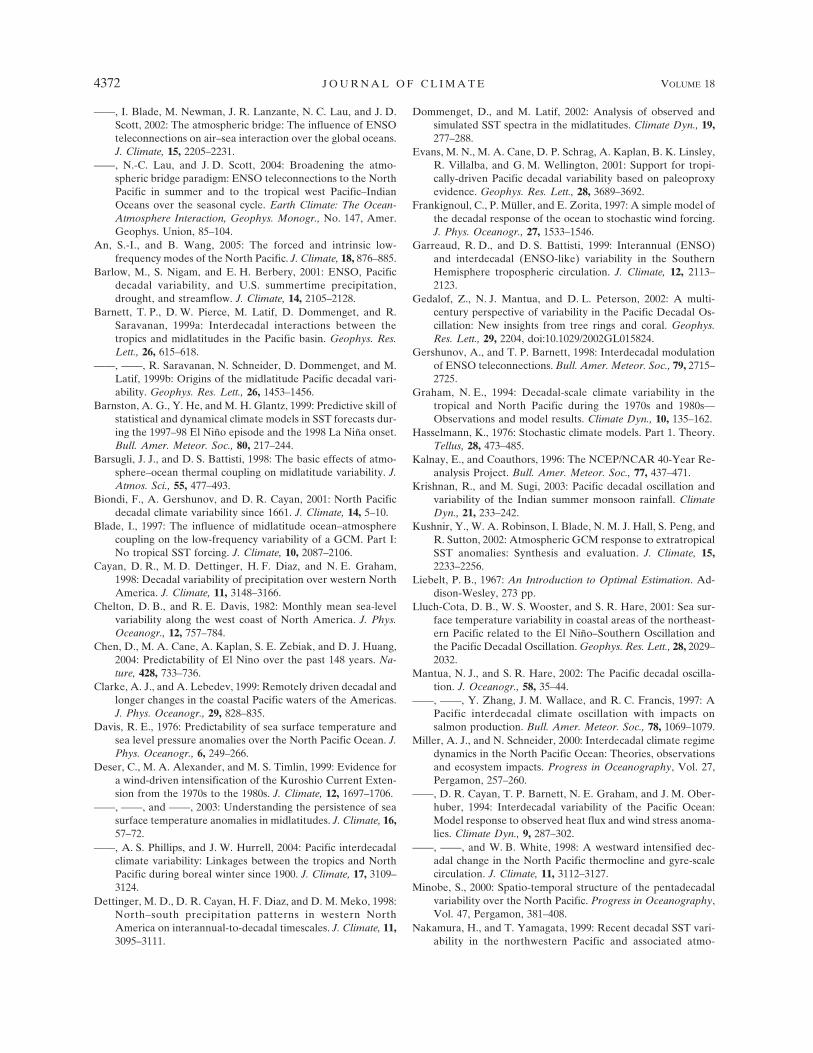
The autocorrelation function of simulated T hasthe characteristic structure of reemergence. While forthe reference case the autocorrelation is independent ofthe calendar month, shallow summer mixed layers re-sult in an autocorrelation for winter months that havesecondary peaks in subsequent winters (Fig. B1). Thesesecondary peaks are exacerbated for shallower summermixed layers because the heat anomaly in the seasonalthermocline is larger relative to the heat anomalystored in the summer mixed layer.

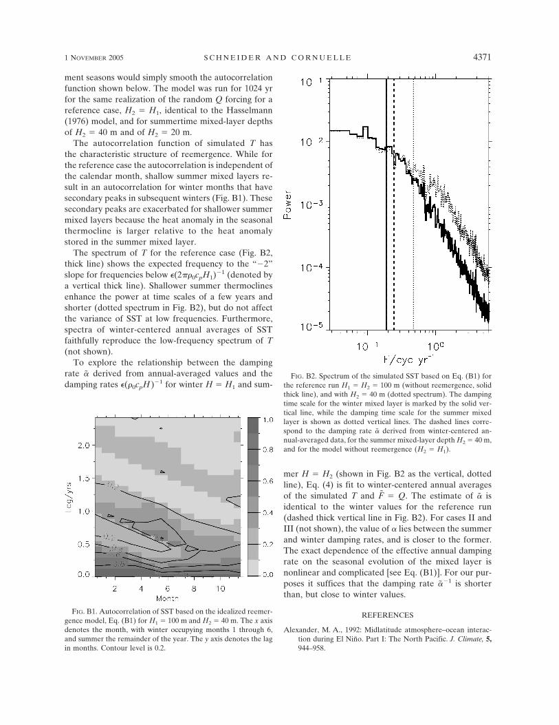
The spectrum of T for the reference case (Fig. B2,thick line) shows the expected frequency to the “�2”slope for frequencies below �(2� 0cpH1)�1 (denoted bya vertical thick line). Shallower summer thermoclinesenhance the power at time scales of a few years andshorter (dotted spectrum in Fig. B2), but do not affectthe variance of SST at low frequencies. Furthermore,spectra of winter-centered annual averages of SSTfaithfully reproduce the low-frequency spectrum of T(not shown).

To explore the relationship between the dampingrate � derived from annual-averaged values and thedamping rates �( 0cpH)�1 for winter H � H1 and sum-

mer H � H2 (shown in Fig. B2 as the vertical, dottedline), Eq. (4) is fit to winter-centered annual averagesof the simulated T and F � Q. The estimate of � isidentical to the winter values for the reference run(dashed thick vertical line in Fig. B2). For cases II andIII (not shown), the value of � lies between the summerand winter damping rates, and is closer to the former.The exact dependence of the effective annual dampingrate on the seasonal evolution of the mixed layer isnonlinear and complicated [see Eq. (B1)]. For our pur-poses it suffices that the damping rate ��1 is shorterthan, but close to winter values.

REFERENCES

Alexander, M. A., 1992: Midlatitude atmosphere–ocean interac-tion during El Niño. Part I: The North Pacific. J. Climate, 5,944–958.

FIG. B1. Autocorrelation of SST based on the idealized reemer-gence model, Eq. (B1) for H1 � 100 m and H2 � 40 m. The x axisdenotes the month, with winter occupying months 1 through 6,and summer the remainder of the year. The y axis denotes the lagin months. Contour level is 0.2.

FIG. B2. Spectrum of the simulated SST based on Eq. (B1) forthe reference run H1 � H2 � 100 m (without reemergence, solidthick line), and with H2 � 40 m (dotted spectrum). The dampingtime scale for the winter mixed layer is marked by the solid ver-tical line, while the damping time scale for the summer mixedlayer is shown as dotted vertical lines. The dashed lines corre-spond to the damping rate � derived from winter-centered an-nual-averaged data, for the summer mixed-layer depth H2 � 40 m,and for the model without reemergence (H2 � H1).


——, I. Blade, M. Newman, J. R. Lanzante, N. C. Lau, and J. D.Scott, 2002: The atmospheric bridge: The influence of ENSOteleconnections on air–sea interaction over the global oceans.J. Climate, 15, 2205–2231.

——, N.-C. Lau, and J. D. Scott, 2004: Broadening the atmo-spheric bridge paradigm: ENSO teleconnections to the NorthPacific in summer and to the tropical west Pacific–IndianOceans over the seasonal cycle. Earth Climate: The Ocean-Atmosphere Interaction, Geophys. Monogr., No. 147, Amer.Geophys. Union, 85–104.

An, S.-I., and B. Wang, 2005: The forced and intrinsic low-frequency modes of the North Pacific. J. Climate, 18, 876–885.

Barlow, M., S. Nigam, and E. H. Berbery, 2001: ENSO, Pacificdecadal variability, and U.S. summertime precipitation,drought, and streamflow. J. Climate, 14, 2105–2128.

Barnett, T. P., D. W. Pierce, M. Latif, D. Dommenget, and R.Saravanan, 1999a: Interdecadal interactions between thetropics and midlatitudes in the Pacific basin. Geophys. Res.Lett., 26, 615–618.

——, ——, R. Saravanan, N. Schneider, D. Dommenget, and M.Latif, 1999b: Origins of the midlatitude Pacific decadal vari-ability. Geophys. Res. Lett., 26, 1453–1456.

Barnston, A. G., Y. He, and M. H. Glantz, 1999: Predictive skill ofstatistical and dynamical climate models in SST forecasts dur-ing the 1997–98 El Niño episode and the 1998 La Niña onset.Bull. Amer. Meteor. Soc., 80, 217–244.

Barsugli, J. J., and D. S. Battisti, 1998: The basic effects of atmo-sphere–ocean thermal coupling on midlatitude variability. J.Atmos. Sci., 55, 477–493.

Biondi, F., A. Gershunov, and D. R. Cayan, 2001: North Pacificdecadal climate variability since 1661. J. Climate, 14, 5–10.

Blade, I., 1997: The influence of midlatitude ocean–atmospherecoupling on the low-frequency variability of a GCM. Part I:No tropical SST forcing. J. Climate, 10, 2087–2106.

Cayan, D. R., M. D. Dettinger, H. F. Diaz, and N. E. Graham,1998: Decadal variability of precipitation over western NorthAmerica. J. Climate, 11, 3148–3166.

Chelton, D. B., and R. E. Davis, 1982: Monthly mean sea-levelvariability along the west coast of North America. J. Phys.Oceanogr., 12, 757–784.

Chen, D., M. A. Cane, A. Kaplan, S. E. Zebiak, and D. J. Huang,2004: Predictability of El Nino over the past 148 years. Na-ture, 428, 733–736.

Clarke, A. J., and A. Lebedev, 1999: Remotely driven decadal andlonger changes in the coastal Pacific waters of the Americas.J. Phys. Oceanogr., 29, 828–835.

Davis, R. E., 1976: Predictability of sea surface temperature andsea level pressure anomalies over the North Pacific Ocean. J.Phys. Oceanogr., 6, 249–266.

Deser, C., M. A. Alexander, and M. S. Timlin, 1999: Evidence fora wind-driven intensification of the Kuroshio Current Exten-sion from the 1970s to the 1980s. J. Climate, 12, 1697–1706.

——, ——, and ——, 2003: Understanding the persistence of seasurface temperature anomalies in midlatitudes. J. Climate, 16,57–72.

——, A. S. Phillips, and J. W. Hurrell, 2004: Pacific interdecadalclimate variability: Linkages between the tropics and NorthPacific during boreal winter since 1900. J. Climate, 17, 3109–3124.

Dettinger, M. D., D. R. Cayan, H. F. Diaz, and D. M. Meko, 1998:North–south precipitation patterns in western NorthAmerica on interannual-to-decadal timescales. J. Climate, 11,3095–3111.

Dommenget, D., and M. Latif, 2002: Analysis of observed andsimulated SST spectra in the midlatitudes. Climate Dyn., 19,277–288.

Evans, M. N., M. A. Cane, D. P. Schrag, A. Kaplan, B. K. Linsley,R. Villalba, and G. M. Wellington, 2001: Support for tropi-cally-driven Pacific decadal variability based on paleoproxyevidence. Geophys. Res. Lett., 28, 3689–3692.

Frankignoul, C., P. Müller, and E. Zorita, 1997: A simple model ofthe decadal response of the ocean to stochastic wind forcing.J. Phys. Oceanogr., 27, 1533–1546.

Garreaud, R. D., and D. S. Battisti, 1999: Interannual (ENSO)and interdecadal (ENSO-like) variability in the SouthernHemisphere tropospheric circulation. J. Climate, 12, 2113–2123.

Gedalof, Z., N. J. Mantua, and D. L. Peterson, 2002: A multi-century perspective of variability in the Pacific Decadal Os-cillation: New insights from tree rings and coral. Geophys.Res. Lett., 29, 2204, doi:10.1029/2002GL015824.

Gershunov, A., and T. P. Barnett, 1998: Interdecadal modulationof ENSO teleconnections. Bull. Amer. Meteor. Soc., 79, 2715–2725.

Graham, N. E., 1994: Decadal-scale climate variability in thetropical and North Pacific during the 1970s and 1980s—Observations and model results. Climate Dyn., 10, 135–162.

Hasselmann, K., 1976: Stochastic climate models. Part 1. Theory.Tellus, 28, 473–485.

Kalnay, E., and Coauthors, 1996: The NCEP/NCAR 40-Year Re-analysis Project. Bull. Amer. Meteor. Soc., 77, 437–471.

Krishnan, R., and M. Sugi, 2003: Pacific decadal oscillation andvariability of the Indian summer monsoon rainfall. ClimateDyn., 21, 233–242.

Kushnir, Y., W. A. Robinson, I. Blade, N. M. J. Hall, S. Peng, andR. Sutton, 2002: Atmospheric GCM response to extratropicalSST anomalies: Synthesis and evaluation. J. Climate, 15,2233–2256.

Liebelt, P. B., 1967: An Introduction to Optimal Estimation. Ad-dison-Wesley, 273 pp.

Lluch-Cota, D. B., W. S. Wooster, and S. R. Hare, 2001: Sea sur-face temperature variability in coastal areas of the northeast-ern Pacific related to the El Niño–Southern Oscillation andthe Pacific Decadal Oscillation. Geophys. Res. Lett., 28, 2029–2032.

Mantua, N. J., and S. R. Hare, 2002: The Pacific decadal oscilla-tion. J. Oceanogr., 58, 35–44.

——, ——, Y. Zhang, J. M. Wallace, and R. C. Francis, 1997: APacific interdecadal climate oscillation with impacts onsalmon production. Bull. Amer. Meteor. Soc., 78, 1069–1079.

Miller, A. J., and N. Schneider, 2000: Interdecadal climate regimedynamics in the North Pacific Ocean: Theories, observationsand ecosystem impacts. Progress in Oceanography, Vol. 27,Pergamon, 257–260.

——, D. R. Cayan, T. P. Barnett, N. E. Graham, and J. M. Ober-huber, 1994: Interdecadal variability of the Pacific Ocean:Model response to observed heat flux and wind stress anoma-lies. Climate Dyn., 9, 287–302.

——, ——, and W. B. White, 1998: A westward intensified dec-adal change in the North Pacific thermocline and gyre-scalecirculation. J. Climate, 11, 3112–3127.

Minobe, S., 2000: Spatio-temporal structure of the pentadecadalvariability over the North Pacific. Progress in Oceanography,Vol. 47, Pergamon, 381–408.

Nakamura, H., and T. Yamagata, 1999: Recent decadal SST vari-ability in the northwestern Pacific and associated atmo-


spheric anomalies. Beyond El Niño: Decadal and Interdec-adal Climate Variability, Springer Verlag, 49–72.

——, and A. S. Kazmin, 2003: Decadal changes in the North Pa-cific oceanic frontal zones as revealed in ship and satelliteobservations. J. Geophys. Res., 108, 3078, doi:10.1029/1999JC000085.

——, G. Lin, and T. Yamagata, 1997: Decadal climate variabilityin the North Pacific during recent decades. Bull. Amer. Me-teor. Soc., 78, 2215–2225.

——, T. Izumi, and T. Sampe, 2002: Interannual and decadalmodulation recently observed in the North Pacific stormtrack activity and east Asian winter monsoon. J. Climate, 15,1855–1874.

Newman, M., G. P. Compo, and M. A. Alexander, 2003: ENSO-forced variability of the Pacific decadal oscillation. J. Climate,16, 3853–3857.

Nitta, T., and S. Yamada, 1989: Recent warming of tropical seasurface temperature and its relationship to the NorthernHemisphere circulation. J. Meteor. Soc. Japan, 67, 375–383.

Pierce, D. W., 2001: Distinguishing coupled ocean–atmosphere in-teractions from background noise in the North Pacific. Prog-ress in Oceanography, Vol. 49, Pergamon, 331–352.

——, 2002: The role of sea surface temperatures in interactionsbetween ENSO and the North Pacific Oscillation. J. Climate,15, 1295–1308.

——, T. Barnett, and M. Latif, 2000: Connections between thePacific Ocean tropics and midlatitudes on decadal timescales. J. Climate, 13, 1173–1194.

——, T. P. Barnett, N. Schneider, R. Saravanan, D. Dommenget,and M. Latif, 2001: The role of ocean dynamics in producingdecadal climate variability in the North Pacific. Climate Dyn.,18, 51–70.

Qiu, B., 2003: Kuroshio Extension variability and forcing of thePacific decadal oscillations: Responses and potential feed-back. J. Phys. Oceanogr., 33, 2465–2482.

Schneider, N., and A. J. Miller, 2001: Predicting western NorthPacific ocean climate. J. Climate, 14, 3997–4002.

——, ——, and D. W. Pierce, 2002: Anatomy of North Pacificdecadal variability. J. Climate, 15, 586–605.

Seager, R., Y. Kushnir, N. Naik, M. A. Cane, and J. A. Miller,2001: Wind-driven shifts in the latitude of the Kuroshio–Oyashio Extension and generation of SST anomalies on dec-adal timescales. J. Climate, 14, 4249–4265.

Sturges, W., and B. G. Hong, 1995: Wind forcing of the Atlanticthermocline along 32°N at low frequencies. J. Phys. Ocean-ogr., 25, 1706–1715.

Tanimoto, Y., H. Nakamura, T. Kagimoto, and S. Yamane, 2003:An active role of extratropical sea surface temperatureanomalies in determining anomalous turbulent heat flux. J.Geophys. Res., 108, 3304, doi:10.1029/2002JC001750.

Tomita, T., B. Wang, T. Yasunari, and H. Nakamura, 2001: Globalpatterns of decadal-scale variability observed in sea surfacetemperature and lower-tropospheric circulation fields. J.Geophys. Res., 106, 26 805–26 815.

Trenberth, K. E., 1990: Recent observed interdecadal climatechanges in the Northern Hemisphere. Bull. Amer. Meteor.Soc., 71, 988–993.

——, and J. W. Hurrell, 1994: Decadal atmosphere–ocean varia-tions in the Pacific. Climate Dyn., 9, 303–319.

Vimont, D. J., D. S. Battisti, and A. C. Hirst, 2001: Footprinting:A seasonal connection between the tropics and mid-latitudes.Geophys. Res. Lett., 28, 3923–3926.

——, ——, and ——, 2003: Seasonal footprinting in the Pacific:Implications for ENSO. J. Climate, 16, 2668–2675.

Xie, S. P., T. Kunitani, A. Kubokawa, M. Nonaka, and S. Hosoda,2000: Interdecadal thermocline variability in the North Pa-cific for 1958–1997: A GCM simulation. J. Phys. Oceanogr.,30, 2798–2813.

Yulaeva, E., N. Schneider, D. W. Pierce, and T. Barnett, 2001:Modeling of North Pacific climate variability forced by oce-anic heat fluxes anomalies. J. Climate, 14, 4027–4046.

Zhang, Y., J. M. Wallace, and D. S. Battisti, 1997: ENSO-like in-terdecadal variability: 1900–93. J. Climate, 10, 1004–1020.


the forcing of the pacific decadal oscillation*

Documents