Degenerate parametric oscillation in quantum membrane optomechanics

Monica Benito,1, 2, ∗ Carlos Sanchez Munoz,3, 2, ∗ and Carlos Navarrete-Benlloch2

1Instituto de Ciencia de Materiales, CSIC, Cantoblanco, 28049 Madrid, Spain2Max-Planck Institut fur Quantenoptik, Hans-Kopfermann-Str. 1, D-85748 Garching, Germany

3Fısica Teorica de la Materia Condensada, Universidad Autonoma de Madrid, 28049 Madrid, Spain

The promise of innovative applications has triggered the development of many modern technolo-gies capable of exploiting quantum effects. But in addition to future applications, such quantumtechnologies have already provided us with the possibility of accessing quantum-mechanical scenariosthat seemed unreachable just a few decades ago. With this spirit, in this work we show that modernoptomechanical setups are mature enough to implement one of the most elusive models in the fieldof open system dynamics: degenerate parametric oscillation. The possibility of implementing it innonlinear optical resonators was the main motivation for introducing such model in the eighties,which rapidly became a paradigm for the study of dissipative phase transitions whose correspond-ing spontaneously broken symmetry is discrete. However, it was found that the intrinsic multimodenature of optical cavities makes it impossible to experimentally study the model all the way throughits phase transition. In contrast, here we show that this long-awaited model can be implemented inthe motion of a mechanical object dispersively coupled to the light contained in a cavity, when thelatter is properly driven with multi-chromatic laser light. We focus on membranes as the mechanicalelement, showing that the main signatures of the degenerate parametric oscillation model can bestudied in state-of-the-art setups, thus opening the possibility of studying spontaneous symmetrybreaking and enhanced metrology in one of the cleanest dissipative phase transitions.

PACS numbers: 42.50.-p,42.65.Yj,42.50.Wk,03.65.Yz

Introduction. The last decades have seen the birthof a plethora of new technologies working in the quantumregime, starting with the laser [1–8], and including non-linear optics [9–13], trapped ions [14–18] and atoms [19–27], cavity quantum electrodynamics [28–31], or, morerecently, superconducting circuits [32–36] and optome-chanical resonators [37–39]. Apart from their potentialfor quantum computation [40–42] and simulation [43–50],quantum metrology [51, 52], and quantum communica-tion [53–55], all these technologies have allowed us toreach physical scenarios that were nothing but a dream(or a ‘gedanken’ experiment) for the founding fathers ofquantum mechanics.

In this work we keep deepening into the possibilityof using new technologies to access phenomena that,even though predicted and theoretically analyzed sincedecades ago, have eluded observation so far, or only untilvery recently [56]. In particular, we show how modern op-tomechanical setups based on oscillating membranes [57–67] allow for the implementation of degenerate paramet-ric oscillation (DPO), a fundamental model in the fieldof dissipative phase transitions [68–72]. Together withthe laser, DPO has possibly the best-studied quantum-optical dissipative model, since it holds the paradigm ofa phase transition whose associated spontaneously bro-ken symmetry is discrete [71, 72] (in contrast to that ofthe laser, which is continuous [73, 74]). Even though themain motivation for studying such a model came fromnonlinear optics during the eighties [12], in particularfrom the possibility of implementing it in optical para-metric oscillators, see Fig. 1, the intrinsic multi-mode na-ture of optical cavities prevents its implementation above

the phase transition, as we explain in the next section.In other words, despite the great deal of work investedon this model and its optical implementation, degener-ate optical parametric oscillators (DOPOs) do not existin reality.

The situation is rather different in the microwave realmof electronic circuits, where one can build single-modecavities in the form of simple LC circuits. Indeed, it is inthis context where DPO has been traditionally studied inmore detail all the way through its phase transition [75–77]. However, an electronic circuit at room temperaturehas a very strong thermal microwave background which,together with other sources of technical noise, completelymasks quantum noise and hence any possibility of analyz-ing quantum mechanical effects. This scenario was radi-cally changed with the advent of superconducting circuits[32–36], which are cooled down to mK temperatures, ef-fectively removing the thermal background and makingit possible to access the quantum regime. It is in this sce-nario where, just a few months ago, quantum mechanicaleffects appearing as one crosses the phase transition ofthe DPO model have been finally observed [56].

Apart from being a clean system where studying fun-damental questions related to spontaneous symmetrybreaking and ergodicity of open quantum systems [78–81], DPO might serve as a perfect test bed for enhancedmetrology via dissipative phase transitions [82–85]. Mo-tivated then by the interest that this model generateson different communities ranging from the purely theo-retical to the most applied ones, in this work we showthat DPO can be implemented in the motion of a mem-brane dispersively coupled to the field of an optical cavity

arX

iv:1

506.

0815

7v1

[qu

ant-

ph]

26

Jun

2015

2

(2)non#resonant)pump)at) down#converted)

field)at)

2!0

/2!0

down#converted)photons)

pump)photons)

g2/4

(a)

p

x

0

10

10

20

20

10.8 1.2 1.4 1.6 1.8 20.60 33 3 30

(b)

2↵

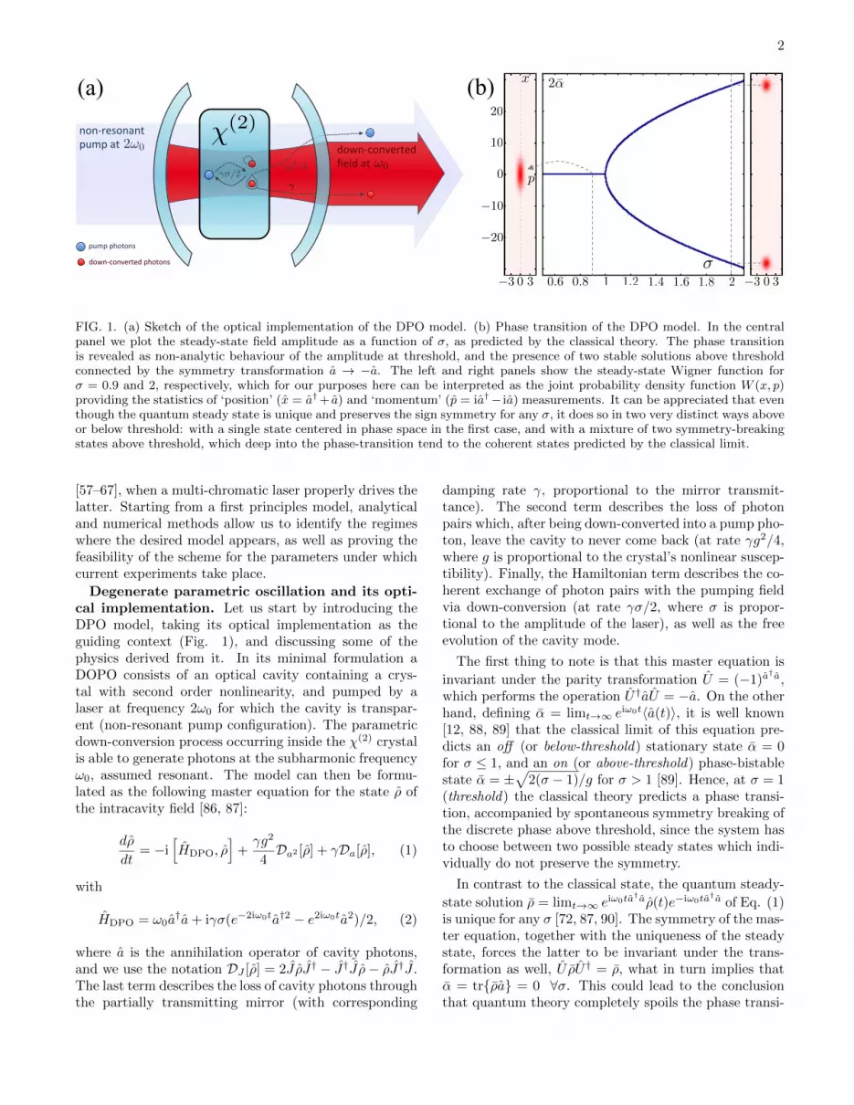
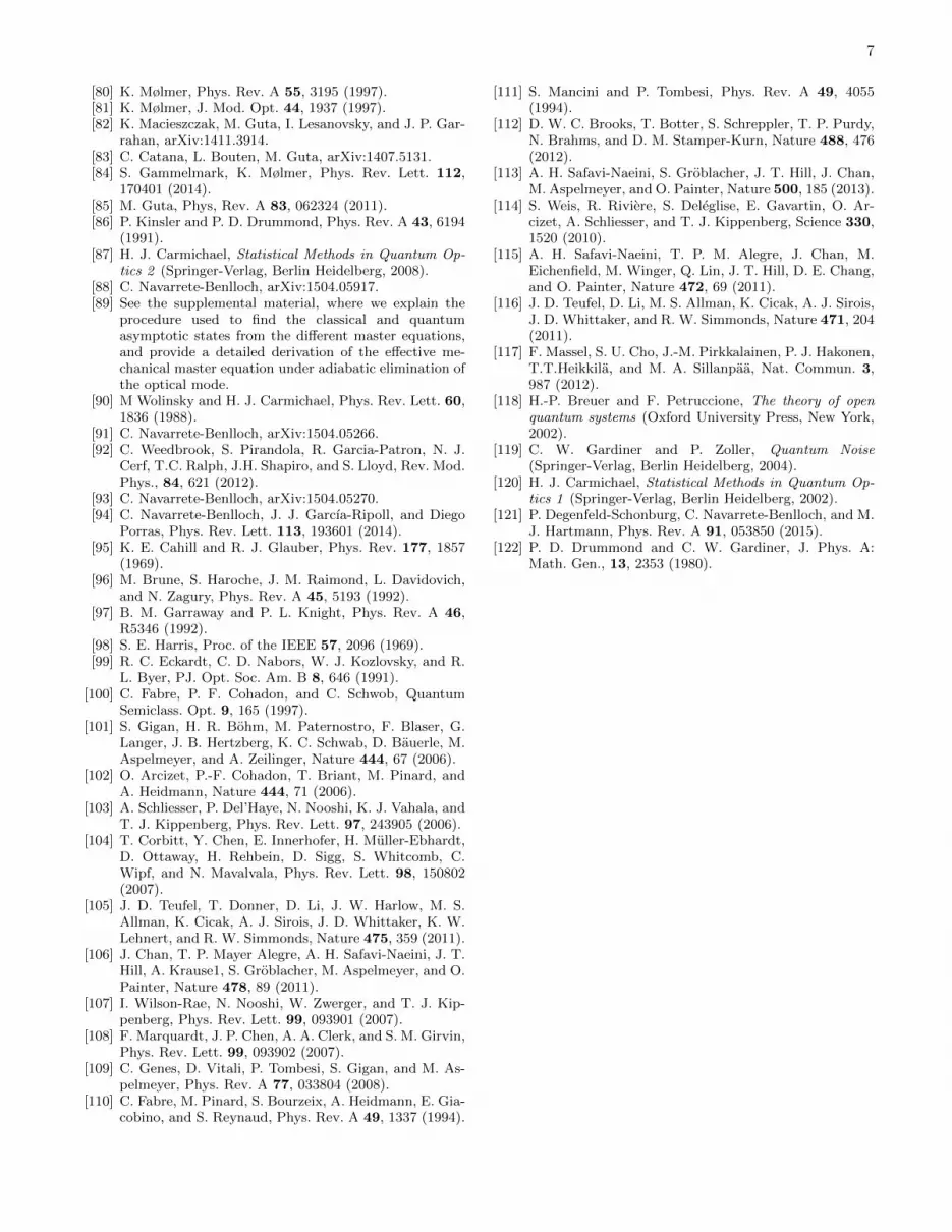
FIG. 1. (a) Sketch of the optical implementation of the DPO model. (b) Phase transition of the DPO model. In the centralpanel we plot the steady-state field amplitude as a function of σ, as predicted by the classical theory. The phase transitionis revealed as non-analytic behaviour of the amplitude at threshold, and the presence of two stable solutions above thresholdconnected by the symmetry transformation a → −a. The left and right panels show the steady-state Wigner function forσ = 0.9 and 2, respectively, which for our purposes here can be interpreted as the joint probability density function W (x, p)providing the statistics of ‘position’ (x = a†+ a) and ‘momentum’ (p = ia†− ia) measurements. It can be appreciated that eventhough the quantum steady state is unique and preserves the sign symmetry for any σ, it does so in two very distinct ways aboveor below threshold: with a single state centered in phase space in the first case, and with a mixture of two symmetry-breakingstates above threshold, which deep into the phase-transition tend to the coherent states predicted by the classical limit.

[57–67], when a multi-chromatic laser properly drives thelatter. Starting from a first principles model, analyticaland numerical methods allow us to identify the regimeswhere the desired model appears, as well as proving thefeasibility of the scheme for the parameters under whichcurrent experiments take place.

Degenerate parametric oscillation and its opti-cal implementation. Let us start by introducing theDPO model, taking its optical implementation as theguiding context (Fig. 1), and discussing some of thephysics derived from it. In its minimal formulation aDOPO consists of an optical cavity containing a crys-tal with second order nonlinearity, and pumped by alaser at frequency 2ω0 for which the cavity is transpar-ent (non-resonant pump configuration). The parametricdown-conversion process occurring inside the χ(2) crystalis able to generate photons at the subharmonic frequencyω0, assumed resonant. The model can then be formu-lated as the following master equation for the state ρ ofthe intracavity field [86, 87]:

dρ

dt= −i

[HDPO, ρ

]+γg2

4Da2 [ρ] + γDa[ρ], (1)

with

HDPO = ω0a†a+ iγσ(e−2iω0ta†2 − e2iω0ta2)/2, (2)

where a is the annihilation operator of cavity photons,and we use the notation DJ [ρ] = 2J ρJ† − J†J ρ− ρJ†J .The last term describes the loss of cavity photons throughthe partially transmitting mirror (with corresponding

damping rate γ, proportional to the mirror transmit-tance). The second term describes the loss of photonpairs which, after being down-converted into a pump pho-ton, leave the cavity to never come back (at rate γg2/4,where g is proportional to the crystal’s nonlinear suscep-tibility). Finally, the Hamiltonian term describes the co-herent exchange of photon pairs with the pumping fieldvia down-conversion (at rate γσ/2, where σ is propor-tional to the amplitude of the laser), as well as the freeevolution of the cavity mode.

The first thing to note is that this master equation is

invariant under the parity transformation U = (−1)a†a,

which performs the operation U†aU = −a. On the otherhand, defining α = limt→∞ eiω0t〈a(t)〉, it is well known[12, 88, 89] that the classical limit of this equation pre-dicts an off (or below-threshold) stationary state α = 0for σ ≤ 1, and an on (or above-threshold) phase-bistablestate α = ±

√2(σ − 1)/g for σ > 1 [89]. Hence, at σ = 1

(threshold) the classical theory predicts a phase transi-tion, accompanied by spontaneous symmetry breaking ofthe discrete phase above threshold, since the system hasto choose between two possible steady states which indi-vidually do not preserve the symmetry.

In contrast to the classical state, the quantum steady-

state solution ρ = limt→∞ eiω0ta†aρ(t)e−iω0ta

†a of Eq. (1)is unique for any σ [72, 87, 90]. The symmetry of the mas-ter equation, together with the uniqueness of the steadystate, forces the latter to be invariant under the trans-formation as well, U ρU† = ρ, what in turn implies thatα = trρa = 0 ∀σ. This could lead to the conclusionthat quantum theory completely spoils the phase transi-

3

quadra&c(mode(

linear(mode(

membrane(

!Q

!L

1 1.2 1.40.80.60.40.2

n

(a) (b)

0

2

4

6

0.6 0.7 0.8 0.90

2

4

!Q q

n 108

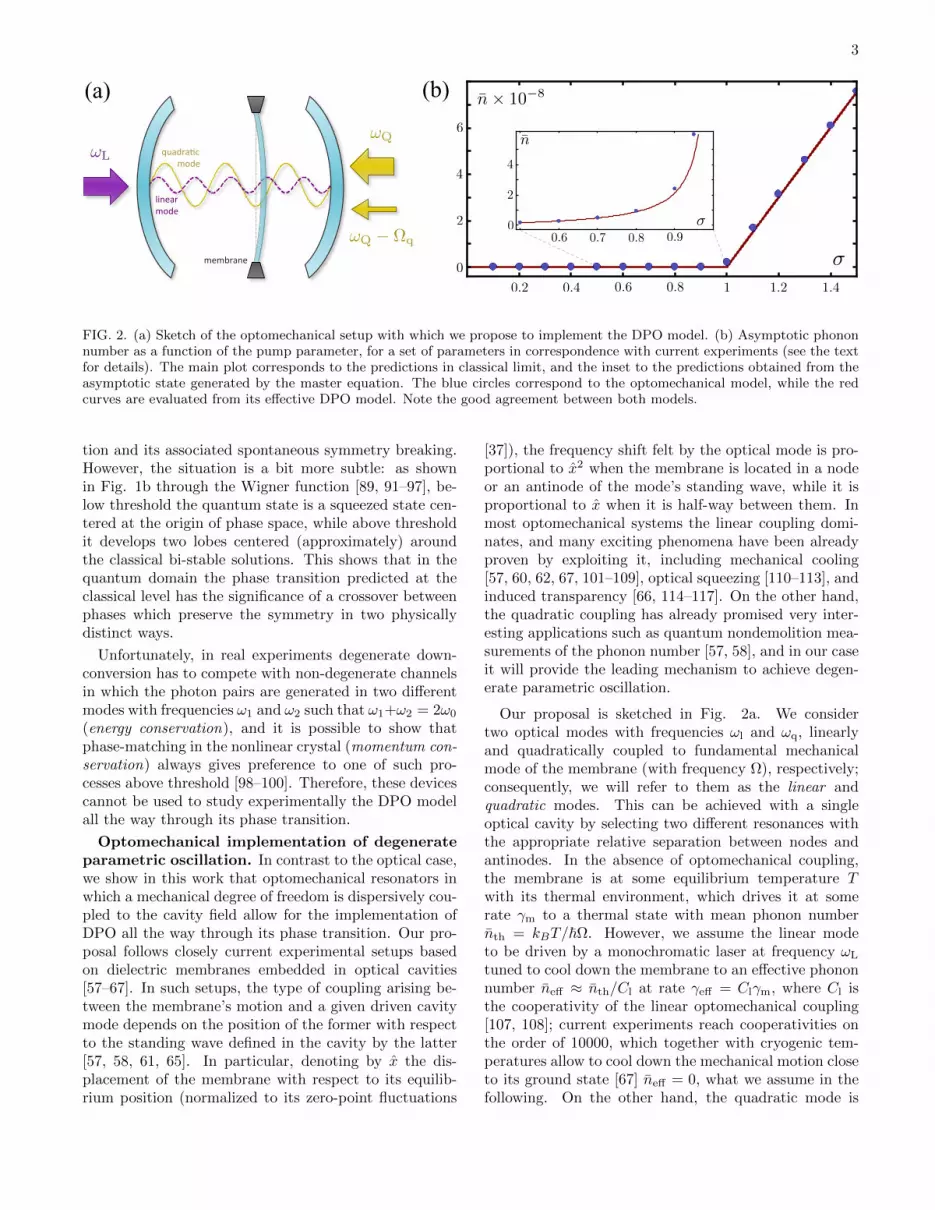
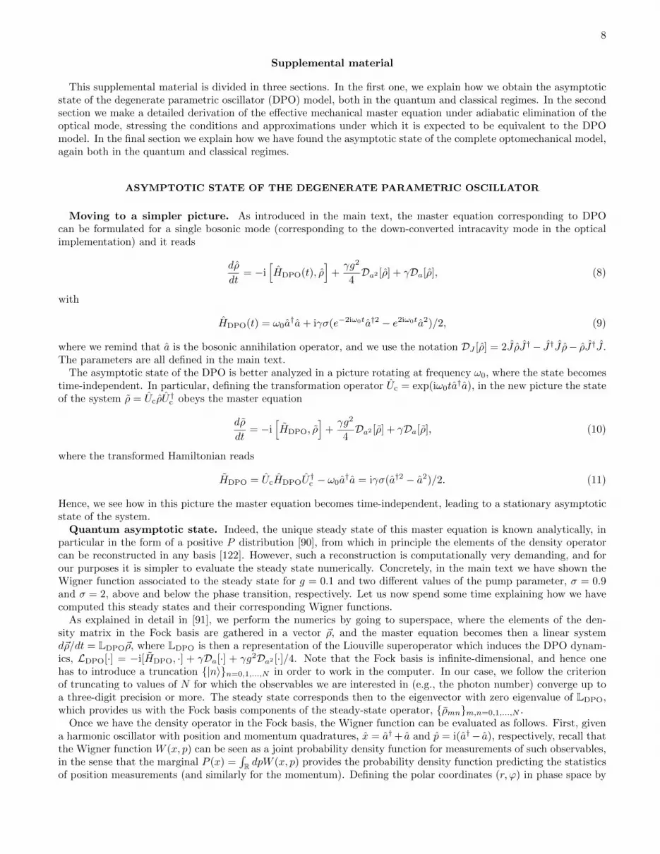
FIG. 2. (a) Sketch of the optomechanical setup with which we propose to implement the DPO model. (b) Asymptotic phononnumber as a function of the pump parameter, for a set of parameters in correspondence with current experiments (see the textfor details). The main plot corresponds to the predictions in classical limit, and the inset to the predictions obtained from theasymptotic state generated by the master equation. The blue circles correspond to the optomechanical model, while the redcurves are evaluated from its effective DPO model. Note the good agreement between both models.

tion and its associated spontaneous symmetry breaking.However, the situation is a bit more subtle: as shownin Fig. 1b through the Wigner function [89, 91–97], be-low threshold the quantum state is a squeezed state cen-tered at the origin of phase space, while above thresholdit develops two lobes centered (approximately) aroundthe classical bi-stable solutions. This shows that in thequantum domain the phase transition predicted at theclassical level has the significance of a crossover betweenphases which preserve the symmetry in two physicallydistinct ways.

Unfortunately, in real experiments degenerate down-conversion has to compete with non-degenerate channelsin which the photon pairs are generated in two differentmodes with frequencies ω1 and ω2 such that ω1+ω2 = 2ω0

(energy conservation), and it is possible to show thatphase-matching in the nonlinear crystal (momentum con-servation) always gives preference to one of such pro-cesses above threshold [98–100]. Therefore, these devicescannot be used to study experimentally the DPO modelall the way through its phase transition.

Optomechanical implementation of degenerateparametric oscillation. In contrast to the optical case,we show in this work that optomechanical resonators inwhich a mechanical degree of freedom is dispersively cou-pled to the cavity field allow for the implementation ofDPO all the way through its phase transition. Our pro-posal follows closely current experimental setups basedon dielectric membranes embedded in optical cavities[57–67]. In such setups, the type of coupling arising be-tween the membrane’s motion and a given driven cavitymode depends on the position of the former with respectto the standing wave defined in the cavity by the latter[57, 58, 61, 65]. In particular, denoting by x the dis-placement of the membrane with respect to its equilib-rium position (normalized to its zero-point fluctuations

[37]), the frequency shift felt by the optical mode is pro-portional to x2 when the membrane is located in a nodeor an antinode of the mode’s standing wave, while it isproportional to x when it is half-way between them. Inmost optomechanical systems the linear coupling domi-nates, and many exciting phenomena have been alreadyproven by exploiting it, including mechanical cooling[57, 60, 62, 67, 101–109], optical squeezing [110–113], andinduced transparency [66, 114–117]. On the other hand,the quadratic coupling has already promised very inter-esting applications such as quantum nondemolition mea-surements of the phonon number [57, 58], and in our caseit will provide the leading mechanism to achieve degen-erate parametric oscillation.

Our proposal is sketched in Fig. 2a. We considertwo optical modes with frequencies ωl and ωq, linearlyand quadratically coupled to fundamental mechanicalmode of the membrane (with frequency Ω), respectively;consequently, we will refer to them as the linear andquadratic modes. This can be achieved with a singleoptical cavity by selecting two different resonances withthe appropriate relative separation between nodes andantinodes. In the absence of optomechanical coupling,the membrane is at some equilibrium temperature Twith its thermal environment, which drives it at somerate γm to a thermal state with mean phonon numbernth = kBT/~Ω. However, we assume the linear modeto be driven by a monochromatic laser at frequency ωL

tuned to cool down the membrane to an effective phononnumber neff ≈ nth/Cl at rate γeff = Clγm, where Cl isthe cooperativity of the linear optomechanical coupling[107, 108]; current experiments reach cooperativities onthe order of 10000, which together with cryogenic tem-peratures allow to cool down the mechanical motion closeto its ground state [67] neff = 0, what we assume in thefollowing. On the other hand, the quadratic mode is

4

driven with a laser containing a tone at frequency ωQ,plus a sideband at frequency ωQ − Ωq. We will use thefirst tone to create the two-phonon losses needed in theDPO model (1), while the combined action of the twotones will provide the coherent exchange of phonon pairs.

We model the system by a master equation governingthe evolution of its state ρ, which in a frame rotating atthe laser frequency ωQ takes the form

dρ

dt= −i[Hm+Hq(t)+Hqm, ρ]+γqDaq [ρ]+γeffDb[ρ], (3)

with Hamiltonian terms

Hm = Ωb†b, (4a)

Hq = ∆qa†qaq + i[Eq(t)a†q − E∗q (t)aq], (4b)

Hqm = −gqx2a†qaq, (4c)

where the bichromatic driving amplitude of the quadraticmode can be written as Eq(t) = E0 + E1e−iΩqt+iφ, with φsome relative phase between the two tones. ∆q = ωQ−ωq

is the laser detuning. b is the mechanical annihilation op-erator, from which the mechanical displacement is writ-ten as x = b + b†. aq is the quadratic mode’s an-nihilation operator, with corresponding cavity dampingrate γq (proportional to the mirror transmissivity). Thedriving amplitudes E0,1 can be written in terms of thepower P0,1 of the laser at the corresponding frequency as

E0,1 ≈√

2γqP0,1/~ωq [88].We can understand the conditions under which this

bichromatically-driven optomechanical model is mappedto the DPO model by adiabatically eliminating thequadratic mode. We provide the details of the deriva-tion in [89], and here we just want to point out somephysically relevant steps. We follow the usual projector-superoperator technique [118–121] in which the quadraticmode is assumed to be in some reference state and followsome reference dynamics. For our current purposes, it isenough to assume that it does not feel any mechanicalbackaction, so that its dynamics is described by the mas-ter equation above with gq = 0. This means that: (i) wecan take a coherent state with amplitude

αq(t) = eiarctan(∆q/γq)[√n0 − i

√n1e−iΩQt] (5)

as its reference state, where we have made a concretechoice of the second tone’s phase φ that simplifies theexpression [89], and defined nj = E2

j /[γ2q + (∆q + jΩq)2],

which are interpreted as the number of photons intro-duced by the corresponding laser in the cavity; and (ii)all the correlation functions of its quantum fluctuationsδaq = aq − αq will decay in time at rate γq.

Keeping in mind the traditional picture of sidebandcooling [107–109], it is intuitive to understand how theDPO model arises from Hqm upon adiabatic eliminationof the optical mode. First, it will turn out to be conve-nient to work in the weak sideband regime n1 n0 [89].

The coherent part of the optical field generates then aneffective mechanical Hamiltonian

Heff = Ωb†b− gq|αq(t)|2x2 (6)

≈ Ωeff b†b+ igq

√n0n1(eiΩqtb2 −H.c.),

where Ωeff = Ω − 2gqn0, and any other term can beneglected as long as we work within the rotating-waveapproximation Ωeff gqn0 [89]. Provided that thesecond tone is chosen as Ωq = 2Ωeff , this effective

Hamiltonian provides precisely HDPO as introduced in(2). On the other hand, the elimination of the opti-cal fluctuations generates both dissipative and Hamil-tonian mechanical terms. Within the weak sidebandand rotating-wave approximations, all the Hamiltonianterms can be neglected, while only the dissipators Db2 ,Db†2 , and Db†b, survive, corresponding, respectively, totwo-phonon cooling, heating, and dephasing. In theweak sideband regime, the rate of each process is staticand solely controlled by the fundamental tone. Hence,setting its detuning to the red two-phonon resonance,∆q = −2Ωeff , while working in the resolved sidebandregime, 4Ω2

eff γ2q , the heating and dephasing terms are

highly suppressed [89] just as in standard cooling [107–109], leaving us with a two-photon cooling dissipator atrate γmCq, where we have introduced the cooperativ-ity Cq = g2

qn0/γqγm. It is important to note that theMarkov approximation (central to this method), requiresa decay of the optical correlators much faster than the ef-fective mechanical dynamics induced by the optical fields[89], that is, γq maxγeff , γmCq, gq

√n0n1.

This shows that the dynamics of the mechanical modeshould follow an effective DPO master equation of theform (1), with ω0 = Ωeff , γ = γeff , g2 = 4Cq/Cl, and

σ = g√n1γq/γeff . Remarkably, we obtain a set of pa-

rameters that can be optically tuned by means of thetwo laser powers P0 and P1 and that, as we will showbelow, allow to explore physical regimes not available inall-optical implementations. In the following we discusswhether the parameters which can be reached in currentexperimental setups, together with the bounds that theabove-mentioned conditions impose on these, are com-patible with having a reasonable range for these effectiveDPO parameters.

Implementability in current setups. We take theexperiments of [67] as a reference, in which Ω = 4.4MHz,γm = 0.8Hz, ωq = 1770THz, γq = 1.3MHz, Cl = 10000,and gq = 10−5Hz (this last parameter taken from [65]).In order to stay safely within the rotating-wave approxi-mation we must impose a bound on the intracavity pho-ton number given by n0 Ω/2gq ≈ 1011, what alsocertifies that we are within the resolved sideband regime,Ωeff/γq ≈ 3.5. Taking n0 = 3.3×109 (corresponding to apower of P0 ≈ 20mW, fairly reasonable in such setups),we then obtain a quadratic cooperativity Cq ≈ 3.3×10−7,leading to an effective two-phonon loss g ≈ 10−5, on the

5

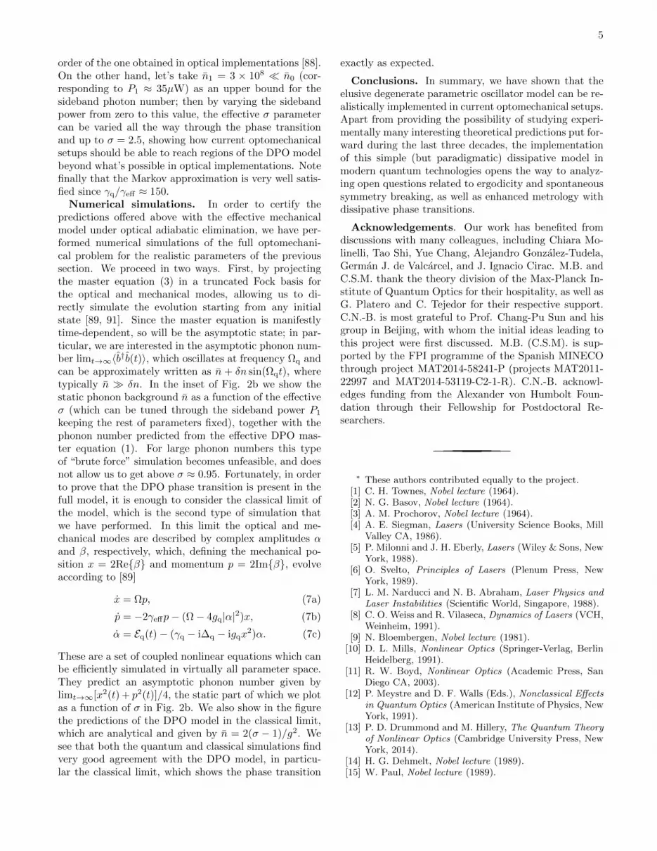
order of the one obtained in optical implementations [88].On the other hand, let’s take n1 = 3 × 108 n0 (cor-responding to P1 ≈ 35µW) as an upper bound for thesideband photon number; then by varying the sidebandpower from zero to this value, the effective σ parametercan be varied all the way through the phase transitionand up to σ = 2.5, showing how current optomechanicalsetups should be able to reach regions of the DPO modelbeyond what’s possible in optical implementations. Notefinally that the Markov approximation is very well satis-fied since γq/γeff ≈ 150.

Numerical simulations. In order to certify thepredictions offered above with the effective mechanicalmodel under optical adiabatic elimination, we have per-formed numerical simulations of the full optomechani-cal problem for the realistic parameters of the previoussection. We proceed in two ways. First, by projectingthe master equation (3) in a truncated Fock basis forthe optical and mechanical modes, allowing us to di-rectly simulate the evolution starting from any initialstate [89, 91]. Since the master equation is manifestlytime-dependent, so will be the asymptotic state; in par-ticular, we are interested in the asymptotic phonon num-ber limt→∞〈b†b(t)〉, which oscillates at frequency Ωq andcan be approximately written as n + δn sin(Ωqt), wheretypically n δn. In the inset of Fig. 2b we show thestatic phonon background n as a function of the effectiveσ (which can be tuned through the sideband power P1

keeping the rest of parameters fixed), together with thephonon number predicted from the effective DPO mas-ter equation (1). For large phonon numbers this typeof “brute force” simulation becomes unfeasible, and doesnot allow us to get above σ ≈ 0.95. Fortunately, in orderto prove that the DPO phase transition is present in thefull model, it is enough to consider the classical limit ofthe model, which is the second type of simulation thatwe have performed. In this limit the optical and me-chanical modes are described by complex amplitudes αand β, respectively, which, defining the mechanical po-sition x = 2Reβ and momentum p = 2Imβ, evolveaccording to [89]

x = Ωp, (7a)

p = −2γeffp− (Ω− 4gq|α|2)x, (7b)

α = Eq(t)− (γq − i∆q − igqx2)α. (7c)

These are a set of coupled nonlinear equations which canbe efficiently simulated in virtually all parameter space.They predict an asymptotic phonon number given bylimt→∞[x2(t) + p2(t)]/4, the static part of which we plotas a function of σ in Fig. 2b. We also show in the figurethe predictions of the DPO model in the classical limit,which are analytical and given by n = 2(σ − 1)/g2. Wesee that both the quantum and classical simulations findvery good agreement with the DPO model, in particu-lar the classical limit, which shows the phase transition

exactly as expected.

Conclusions. In summary, we have shown that theelusive degenerate parametric oscillator model can be re-alistically implemented in current optomechanical setups.Apart from providing the possibility of studying experi-mentally many interesting theoretical predictions put for-ward during the last three decades, the implementationof this simple (but paradigmatic) dissipative model inmodern quantum technologies opens the way to analyz-ing open questions related to ergodicity and spontaneoussymmetry breaking, as well as enhanced metrology withdissipative phase transitions.

Acknowledgements. Our work has benefited fromdiscussions with many colleagues, including Chiara Mo-linelli, Tao Shi, Yue Chang, Alejandro Gonzalez-Tudela,German J. de Valcarcel, and J. Ignacio Cirac. M.B. andC.S.M. thank the theory division of the Max-Planck In-stitute of Quantum Optics for their hospitality, as well asG. Platero and C. Tejedor for their respective support.C.N.-B. is most grateful to Prof. Chang-Pu Sun and hisgroup in Beijing, with whom the initial ideas leading tothis project were first discussed. M.B. (C.S.M). is sup-ported by the FPI programme of the Spanish MINECOthrough project MAT2014-58241-P (projects MAT2011-22997 and MAT2014-53119-C2-1-R). C.N.-B. acknowl-edges funding from the Alexander von Humbolt Foun-dation through their Fellowship for Postdoctoral Re-searchers.

∗ These authors contributed equally to the project.[1] C. H. Townes, Nobel lecture (1964).[2] N. G. Basov, Nobel lecture (1964).[3] A. M. Prochorov, Nobel lecture (1964).[4] A. E. Siegman, Lasers (University Science Books, Mill

Valley CA, 1986).[5] P. Milonni and J. H. Eberly, Lasers (Wiley & Sons, New

York, 1988).[6] O. Svelto, Principles of Lasers (Plenum Press, New

York, 1989).[7] L. M. Narducci and N. B. Abraham, Laser Physics and

Laser Instabilities (Scientific World, Singapore, 1988).[8] C. O. Weiss and R. Vilaseca, Dynamics of Lasers (VCH,

Weinheim, 1991).[9] N. Bloembergen, Nobel lecture (1981).

[10] D. L. Mills, Nonlinear Optics (Springer-Verlag, BerlinHeidelberg, 1991).

[11] R. W. Boyd, Nonlinear Optics (Academic Press, SanDiego CA, 2003).

[12] P. Meystre and D. F. Walls (Eds.), Nonclassical Effectsin Quantum Optics (American Institute of Physics, NewYork, 1991).

[13] P. D. Drummond and M. Hillery, The Quantum Theoryof Nonlinear Optics (Cambridge University Press, NewYork, 2014).

[14] H. G. Dehmelt, Nobel lecture (1989).[15] W. Paul, Nobel lecture (1989).

6

[16] D. J. Wineland, Nobel lecture (2012).[17] D. Leibfried, R. Blatt, C. Monroe, and D. Wineland,

Rev. Mod. Phys. 75, 281 (2003)[18] Ch. Schneider, D. Porras, and T. Schaetz, Rep. Prog.

Phys. 75, 024401 (2012).[19] S. Chu, Nobel lecture (1997).[20] C. N. Cohen-Tannoudji, Nobel lecture (1997).[21] W. D. Phillips, Nobel lecture (1997).[22] W. Ketterle, Nobel lecture (2001).[23] E. A. Cornell and C. E. Wieman, Nobel lecture (2001).[24] H. J. Metcalf and P. van der Straten, Laser Cooling and

Trapping (Springer-Verlag, New York, 1999).[25] A. Ashkin, Optical Trapping and Manipulation of Neu-

tral Particles Using Lasers (World Scientific, Singapore,2006).

[26] D. Jaksch and P. Zoller, Annals of Physics 315, 52(2005).

[27] I. Bloch, J. Dalibard, and W. Zwerger, Rev. Mod. Phys.80, 885 (2008).

[28] S. Haroche, Nobel lecture (2012).[29] J. M. Raimond, M. Brune, and S. Haroche, Rev. Mod.

Phys. 73, 565 (2001).[30] R. Miller, T. E. Northup, K. M. Birnbaum, A. Boca, A.

D. Boozer and H. J. Kimble, J. Phys. B: At. Mol. Opt.Phys. 38, S551 (2005).

[31] H. Walther, B. T. H. Varcoe, B.-G. Englert, and Th.Becker, Rep. Prog. Phys. 69, 1325 (2006).

[32] M. H. Devoret and R. J. Schoelkopf, Science 339, 1169(2012).

[33] R. J. Schoelkopf and S. M. Girvin, Nature 451, 664(2008).

[34] J. Clarke, F. K. Wilhelm, Nature 453, 1031 (2008).[35] J. Q. You and F. Nori, Phys. Today 58, 42 (2005).[36] M. H. Devoret and J. M. Martinis, Quant. Inf. Proc. 3,

381 (2004).[37] M. Aspelmeyer, T. J. Kippenberg, and F. Marquardt,

Rev. Mod. Phys. 86, 1391 (2014).[38] F. Marquardt and S. M. Girvin, Physics 2, 40 (2009).[39] T. J. Kippenberg and K. J. Vahala, Opt. Exp. 15, 17172

(2007).[40] M. A. Nielsen and I. L. Chuang, Quantum Computa-

tion and Quantum Information (Cambridge UniversityPress, New York, 2000).

[41] D. Bacon and W. van Dam, Communications of theACM 53, 84 (2010).

[42] J. Smith and M. Mosca, Algorithms for Quantum Com-puters in Handbook of Natural Computing (Springer,Berlin Heidelberg, 2012).

[43] R. P. Feynman, Engineering and Science 23, 22 (1960).[44] R. P. Feynman, Int. J. Theor. Phys. 21, 467 (1982).[45] S. Lloyd, Science 273, 1073 (1996).[46] J. I. Cirac and P. Zoller, Nature Physics 8, 264 (2012).[47] I. Bloch, J. Dalibard, and S. Nascimbene, Nature

Physics 8, 267 (2012).[48] R. Blatt and C. F. Roos, Nature Physics 8, 277 (2012).[49] A. Aspuru-Guzik and P. Walther, Nature Physics 8, 285

(2012).[50] A. A. Houck, H. E. Tureci, and J. Koch, Nature Physics

8, 292 (2012).[51] V. Giovannetti, S. Lloyd, and L. Maccone, Science 306,

1330 (2004).[52] V. Giovannetti, S. Lloyd, and L. Maccone, Nature Pho-

tonics 5, 222 (2011).[53] N. Gisin, G. Ribordy, W. Tittel, and H. Zbinden, Rev.

Mod. Phys. 74, 145 (2002).[54] N. Gisin and R. Thew, Nature Photonics 1, 165 (2007).[55] N.J. Cerf, G. Leuchs, and E.S. Polzik (Eds.), Quantum

Information with Continuous Variables of Atoms andLight, (Imperial College Press, London, 2007).

[56] Z. Leghtas, S. Touzard, I. M. Pop, A. Kou, B. Vlastakis,A. Petrenko, K. M. Sliwa, A. Narla, S. Shankar, M. J.Hatridge, M. Reagor, L. Frunzio, R. J. Schoelkopf, M.Mirrahimi, M. H. Devoret, Science 347, 853 (2015).

[57] J. D. Thompson, B. M. Zwickl, A. M. Jayich, F. Mar-quardt, S. M. Girvin, and J. G. E. Harris, Nature 452,72 (2008).

[58] A. M. Jayich, J. C. Sankey, B. M. Zwickl, C. Yang, J.D. Thompson, S. M. Girvin, A. A. Clerk, F. Marquardt,and J. G. E. Harris, New J. Phys. 10, 095008 (2008).

[59] B. M. Zwickl, W. E. Shanks, A. M. Jayich, C. Yang,A. C. Bleszynski Jayich, J. D. Thompson, and J. G. E.Harris, App. Phys. Lett. 92, 103125 (2008).

[60] D. J. Wilson, C. A. Regal, S. B. Papp, and H. J. Kimble,Phys. Rev. Lett. 103, 207204 (2009).

[61] J. C. Sankey, C. Yang, B. M. Zwickl, A. M. Jayich, andJ. G. E. Harris, Nat. Phys. 6, 707 (2010).

[62] M. Karuza, C. Molinelli, M. Galassi, C. Biancofiore, R.Natali, P. Tombesi, G. Di Giuseppe, and D. Vitali, NewJ. Phys. 14, 095015 (2012).

[63] T. P. Purdy, R. W. Peterson, P.-L. Yu, and C. A. Regal,New J. of Phys. 14, 115021 (2012).

[64] H. Kaufer, A. Sawadsky, T. Westphal, D. Friedrich1 andR. Schnabel, New J. Phys. 14, 095018 (2012).

[65] M. Karuza, M. Galassi, C. Biancofiore, C. Molinelli, R.Natali, P. Tombesi, G. Di Giuseppe, and D. Vitali, J.Opt. 15, 025704 (2013).

[66] M. Karuza, C. Biancofiore, M. Bawaj, C. Molinelli, M.Galassi, R. Natali, P. Tombesi, G. Di Giuseppe, and D.Vitali, Phys. Rev. A 88, 013804 (2013).

[67] D. Lee, M. Underwood, D. Mason, A. B. Shkarin, K.Borkje, S. M. Girvin, J. G. E. Harris, arXiv:1406.7254.

[68] H. Haken, Synergetics (Springer-Verlag, Berlin Heidel-berg, 1977).

[69] G. Nicolis and I. Prigogine, Self Organization inNonequilibrium Systems (Wiley, New York, 1977).

[70] R. Bonifacio and L. A. Lugiato, Atomic Cooperationin Quantum Optics in Pattern Formation by Dynam-ics Systems and Pattern Recognition (Springer-Verlag,Berlin Heidelberg, 1979).

[71] P. D. Drummond, K. J. McNeil, and D. F. Walls, J.Mod. Opt., 27, 321 (1980).

[72] P. D. Drummond, K. J. McNeil, and D. F. Walls, J.Mod. Opt., 28, 211 (1980).

[73] R. Graham and H. Haken, Z. Phys. 237, 31 (1970).[74] V. Degiorgio and M. O. Scully, Phys. Rev A 2, 1170

(1970).[75] T. Kawakubo, S. Kabashima, and M. Ogishima, J.

Phys. Soc. Japan 34, 1149 (1973).[76] T. Kawakubo, S. Kabashima, and Y. Tsuchiya, Prog.

Theor. Phys. Supplement 64, 150 (1978).[77] S. Kabashima and T. Kawakubo, Phys. Lett. A 70, 375

(1979).[78] R. Graham, Chaos in Dissipative Quantum Systems in

Chaotic Behavior in Quantum Systems (Plenum Press,New Your and London, 1985).

[79] J. D. Cresser, Ergodicity of Quantum Trajectory De-tection Records in Directions in Quantum Optics(Springer-Verlag, Berlin Heidelberg, 2001).

7

[80] K. Mølmer, Phys. Rev. A 55, 3195 (1997).[81] K. Mølmer, J. Mod. Opt. 44, 1937 (1997).[82] K. Macieszczak, M. Guta, I. Lesanovsky, and J. P. Gar-

rahan, arXiv:1411.3914.[83] C. Catana, L. Bouten, M. Guta, arXiv:1407.5131.[84] S. Gammelmark, K. Mølmer, Phys. Rev. Lett. 112,

170401 (2014).[85] M. Guta, Phys, Rev. A 83, 062324 (2011).[86] P. Kinsler and P. D. Drummond, Phys. Rev. A 43, 6194

(1991).[87] H. J. Carmichael, Statistical Methods in Quantum Op-

tics 2 (Springer-Verlag, Berlin Heidelberg, 2008).[88] C. Navarrete-Benlloch, arXiv:1504.05917.[89] See the supplemental material, where we explain the

procedure used to find the classical and quantumasymptotic states from the different master equations,and provide a detailed derivation of the effective me-chanical master equation under adiabatic elimination ofthe optical mode.

[90] M Wolinsky and H. J. Carmichael, Phys. Rev. Lett. 60,1836 (1988).

[91] C. Navarrete-Benlloch, arXiv:1504.05266.[92] C. Weedbrook, S. Pirandola, R. Garcia-Patron, N. J.

Cerf, T.C. Ralph, J.H. Shapiro, and S. Lloyd, Rev. Mod.Phys., 84, 621 (2012).

[93] C. Navarrete-Benlloch, arXiv:1504.05270.[94] C. Navarrete-Benlloch, J. J. Garcıa-Ripoll, and Diego

Porras, Phys. Rev. Lett. 113, 193601 (2014).[95] K. E. Cahill and R. J. Glauber, Phys. Rev. 177, 1857

(1969).[96] M. Brune, S. Haroche, J. M. Raimond, L. Davidovich,

and N. Zagury, Phys. Rev. A 45, 5193 (1992).[97] B. M. Garraway and P. L. Knight, Phys. Rev. A 46,

R5346 (1992).[98] S. E. Harris, Proc. of the IEEE 57, 2096 (1969).[99] R. C. Eckardt, C. D. Nabors, W. J. Kozlovsky, and R.

L. Byer, PJ. Opt. Soc. Am. B 8, 646 (1991).[100] C. Fabre, P. F. Cohadon, and C. Schwob, Quantum

Semiclass. Opt. 9, 165 (1997).[101] S. Gigan, H. R. Bohm, M. Paternostro, F. Blaser, G.

Langer, J. B. Hertzberg, K. C. Schwab, D. Bauerle, M.Aspelmeyer, and A. Zeilinger, Nature 444, 67 (2006).

[102] O. Arcizet, P.-F. Cohadon, T. Briant, M. Pinard, andA. Heidmann, Nature 444, 71 (2006).

[103] A. Schliesser, P. Del’Haye, N. Nooshi, K. J. Vahala, andT. J. Kippenberg, Phys. Rev. Lett. 97, 243905 (2006).

[104] T. Corbitt, Y. Chen, E. Innerhofer, H. Muller-Ebhardt,D. Ottaway, H. Rehbein, D. Sigg, S. Whitcomb, C.Wipf, and N. Mavalvala, Phys. Rev. Lett. 98, 150802(2007).

[105] J. D. Teufel, T. Donner, D. Li, J. W. Harlow, M. S.Allman, K. Cicak, A. J. Sirois, J. D. Whittaker, K. W.Lehnert, and R. W. Simmonds, Nature 475, 359 (2011).

[106] J. Chan, T. P. Mayer Alegre, A. H. Safavi-Naeini, J. T.Hill, A. Krause1, S. Groblacher, M. Aspelmeyer, and O.Painter, Nature 478, 89 (2011).

[107] I. Wilson-Rae, N. Nooshi, W. Zwerger, and T. J. Kip-penberg, Phys. Rev. Lett. 99, 093901 (2007).

[108] F. Marquardt, J. P. Chen, A. A. Clerk, and S. M. Girvin,Phys. Rev. Lett. 99, 093902 (2007).

[109] C. Genes, D. Vitali, P. Tombesi, S. Gigan, and M. As-pelmeyer, Phys. Rev. A 77, 033804 (2008).

[110] C. Fabre, M. Pinard, S. Bourzeix, A. Heidmann, E. Gia-cobino, and S. Reynaud, Phys. Rev. A 49, 1337 (1994).

[111] S. Mancini and P. Tombesi, Phys. Rev. A 49, 4055(1994).

[112] D. W. C. Brooks, T. Botter, S. Schreppler, T. P. Purdy,N. Brahms, and D. M. Stamper-Kurn, Nature 488, 476(2012).

[113] A. H. Safavi-Naeini, S. Groblacher, J. T. Hill, J. Chan,M. Aspelmeyer, and O. Painter, Nature 500, 185 (2013).

[114] S. Weis, R. Riviere, S. Deleglise, E. Gavartin, O. Ar-cizet, A. Schliesser, and T. J. Kippenberg, Science 330,1520 (2010).

[115] A. H. Safavi-Naeini, T. P. M. Alegre, J. Chan, M.Eichenfield, M. Winger, Q. Lin, J. T. Hill, D. E. Chang,and O. Painter, Nature 472, 69 (2011).

[116] J. D. Teufel, D. Li, M. S. Allman, K. Cicak, A. J. Sirois,J. D. Whittaker, and R. W. Simmonds, Nature 471, 204(2011).

[117] F. Massel, S. U. Cho, J.-M. Pirkkalainen, P. J. Hakonen,T.T.Heikkila, and M. A. Sillanpaa, Nat. Commun. 3,987 (2012).

[118] H.-P. Breuer and F. Petruccione, The theory of openquantum systems (Oxford University Press, New York,2002).

[119] C. W. Gardiner and P. Zoller, Quantum Noise(Springer-Verlag, Berlin Heidelberg, 2004).

[120] H. J. Carmichael, Statistical Methods in Quantum Op-tics 1 (Springer-Verlag, Berlin Heidelberg, 2002).

[121] P. Degenfeld-Schonburg, C. Navarrete-Benlloch, and M.J. Hartmann, Phys. Rev. A 91, 053850 (2015).

[122] P. D. Drummond and C. W. Gardiner, J. Phys. A:Math. Gen., 13, 2353 (1980).

8

Supplemental material

This supplemental material is divided in three sections. In the first one, we explain how we obtain the asymptoticstate of the degenerate parametric oscillator (DPO) model, both in the quantum and classical regimes. In the secondsection we make a detailed derivation of the effective mechanical master equation under adiabatic elimination of theoptical mode, stressing the conditions and approximations under which it is expected to be equivalent to the DPOmodel. In the final section we explain how we have found the asymptotic state of the complete optomechanical model,again both in the quantum and classical regimes.

ASYMPTOTIC STATE OF THE DEGENERATE PARAMETRIC OSCILLATOR

Moving to a simpler picture. As introduced in the main text, the master equation corresponding to DPOcan be formulated for a single bosonic mode (corresponding to the down-converted intracavity mode in the opticalimplementation) and it reads

dρ

dt= −i

[HDPO(t), ρ

]+γg2

4Da2 [ρ] + γDa[ρ], (8)

with

HDPO(t) = ω0a†a+ iγσ(e−2iω0ta†2 − e2iω0ta2)/2, (9)

where we remind that a is the bosonic annihilation operator, and we use the notation DJ [ρ] = 2J ρJ†− J†J ρ− ρJ†J .The parameters are all defined in the main text.

The asymptotic state of the DPO is better analyzed in a picture rotating at frequency ω0, where the state becomestime-independent. In particular, defining the transformation operator Uc = exp(iω0ta

†a), in the new picture the stateof the system ρ = UcρU

†c obeys the master equation

dρ

dt= −i

[HDPO, ρ

]+γg2

4Da2 [ρ] + γDa[ρ], (10)

where the transformed Hamiltonian reads

HDPO = UcHDPOU†c − ω0a

†a = iγσ(a†2 − a2)/2. (11)

Hence, we see how in this picture the master equation becomes time-independent, leading to a stationary asymptoticstate of the system.

Quantum asymptotic state. Indeed, the unique steady state of this master equation is known analytically, inparticular in the form of a positive P distribution [90], from which in principle the elements of the density operatorcan be reconstructed in any basis [122]. However, such a reconstruction is computationally very demanding, and forour purposes it is simpler to evaluate the steady state numerically. Concretely, in the main text we have shown theWigner function associated to the steady state for g = 0.1 and two different values of the pump parameter, σ = 0.9and σ = 2, above and below the phase transition, respectively. Let us now spend some time explaining how we havecomputed this steady states and their corresponding Wigner functions.

As explained in detail in [91], we perform the numerics by going to superspace, where the elements of the den-sity matrix in the Fock basis are gathered in a vector ~ρ, and the master equation becomes then a linear systemd~ρ/dt = LDPO~ρ, where LDPO is then a representation of the Liouville superoperator which induces the DPO dynam-ics, LDPO[·] = −i[HDPO, ·] + γDa[·] + γg2Da2 [·]/4. Note that the Fock basis is infinite-dimensional, and hence onehas to introduce a truncation |n〉n=0,1,...,N in order to work in the computer. In our case, we follow the criterionof truncating to values of N for which the observables we are interested in (e.g., the photon number) converge up toa three-digit precision or more. The steady state corresponds then to the eigenvector with zero eigenvalue of LDPO,which provides us with the Fock basis components of the steady-state operator, ρmnm,n=0,1,...,N .

Once we have the density operator in the Fock basis, the Wigner function can be evaluated as follows. First, givena harmonic oscillator with position and momentum quadratures, x = a†+ a and p = i(a†− a), respectively, recall thatthe Wigner function W (x, p) can be seen as a joint probability density function for measurements of such observables,in the sense that the marginal P (x) =

∫R dpW (x, p) provides the probability density function predicting the statistics

of position measurements (and similarly for the momentum). Defining the polar coordinates (r, ϕ) in phase space by

9

(x, p) = r(cosϕ, sinϕ), the Wigner function of the steady state ρ can be found from its components in the Fock basisas [94–97]

W (r, ϕ) =

N∑mn=0

ρmnWmn(r, ϕ), (12)

where we have defined the Wigner function of the operator |m〉〈n|, given by

Wmn(r, ϕ) =(−1)n

π

√n!

m!eiϕ(m−n)rm−nLm−nn (r2)e−r

2/2, (13)

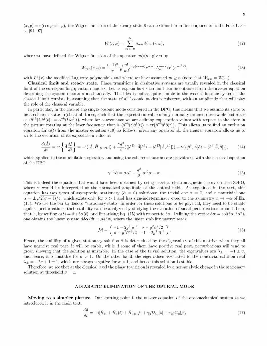
with Lpn(x) the modified Laguerre polynomials and where we have assumed m ≥ n (note that Wnm = W ∗mn).Classical limit and steady state. Phase transitions in dissipative systems are usually revealed in the classical

limit of the corresponding quantum models. Let us explain how such limit can be obtained from the master equationdescribing the system quantum mechanically. The idea is indeed quite simple in the case of bosonic systems: theclassical limit consists in assuming that the state of all bosonic modes is coherent, with an amplitude that will playthe role of the classical variable.

In particular, in the case of the single-bosonic mode considered in the DPO, this means that we assume its state tobe a coherent state |α(t)〉 at all times, such that the expectation value of any normally ordered observable factorizesas 〈a†k(t)al(t)〉 = α∗k(t)αl(t), where for convenience we are defining expectation values with respect to the state inthe picture rotating at the laser frequency, that is 〈a†k(t)al(t)〉 = tra†kalρ(t). This allows us to find an evolutionequation for α(t) from the master equation (10) as follows: given any operator A, the master equation allows us towrite the evolution of its expectation value as

d〈A〉dt

= tr

Adρ

dt

= −i〈[A, HDOPO]〉+

γg2

4(〈[a†2, A]a2〉+ 〈a†2[A, a2]〉) + γ(〈[a†, A]a〉+ 〈a†[A, a]〉), (14)

which applied to the annihilation operator, and using the coherent-state ansatz provides us with the classical equationof the DPO

γ−1α = σα∗ − g2

2|α|2α− α. (15)

This is indeed the equation that would have been obtained by using classical electromagnetic theory on the DOPO,where α would be interpreted as the normalized amplitude of the optical field. As explained in the text, thisequation has two types of asymptotic, stationary (α = 0) solutions: the trivial one α = 0, and a nontrivial oneα = ±

√2(σ − 1)/g, which exists only for σ > 1 and has sign-indeterminacy owed to the symmetry α → −α of Eq.

(15). We use the bar to denote “stationary state” In order for these solutions to be physical, they need to be stableagainst perturbations; their stability can be analyzed by studying the evolution of small perturbations around them,that is, by writing α(t) = α+δα(t), and linearizing Eq. (15) with respect to δα. Defining the vector δα = col(δα, δα∗),one obtains the linear system dδα/dt =Mδα, where the linear stability matrix reads

M =

(−1− 2g2|α|2 σ − g2α2/2σ − g2α∗2/2 −1− 2g2|α|2

). (16)

Hence, the stability of a given stationary solution α is determined by the eigenvalues of this matrix: when they allhave negative real part, it will be stable, while if some of them have positive real part, perturbations will tend togrow, showing that the solution is unstable. In the case of the trivial solution, the eigenvalues are λ± = −1 ± σ,and hence, it is unstable for σ > 1. On the other hand, the eigenvalues associated to the nontrivial solution readλ± = −2σ + 1± 1, which are always negative for σ > 1, and hence this solution is stable.

Therefore, we see that at the classical level the phase transition is revealed by a non-analytic change in the stationarysolution at threshold σ = 1.

ADIABATIC ELIMINATION OF THE OPTICAL MODE

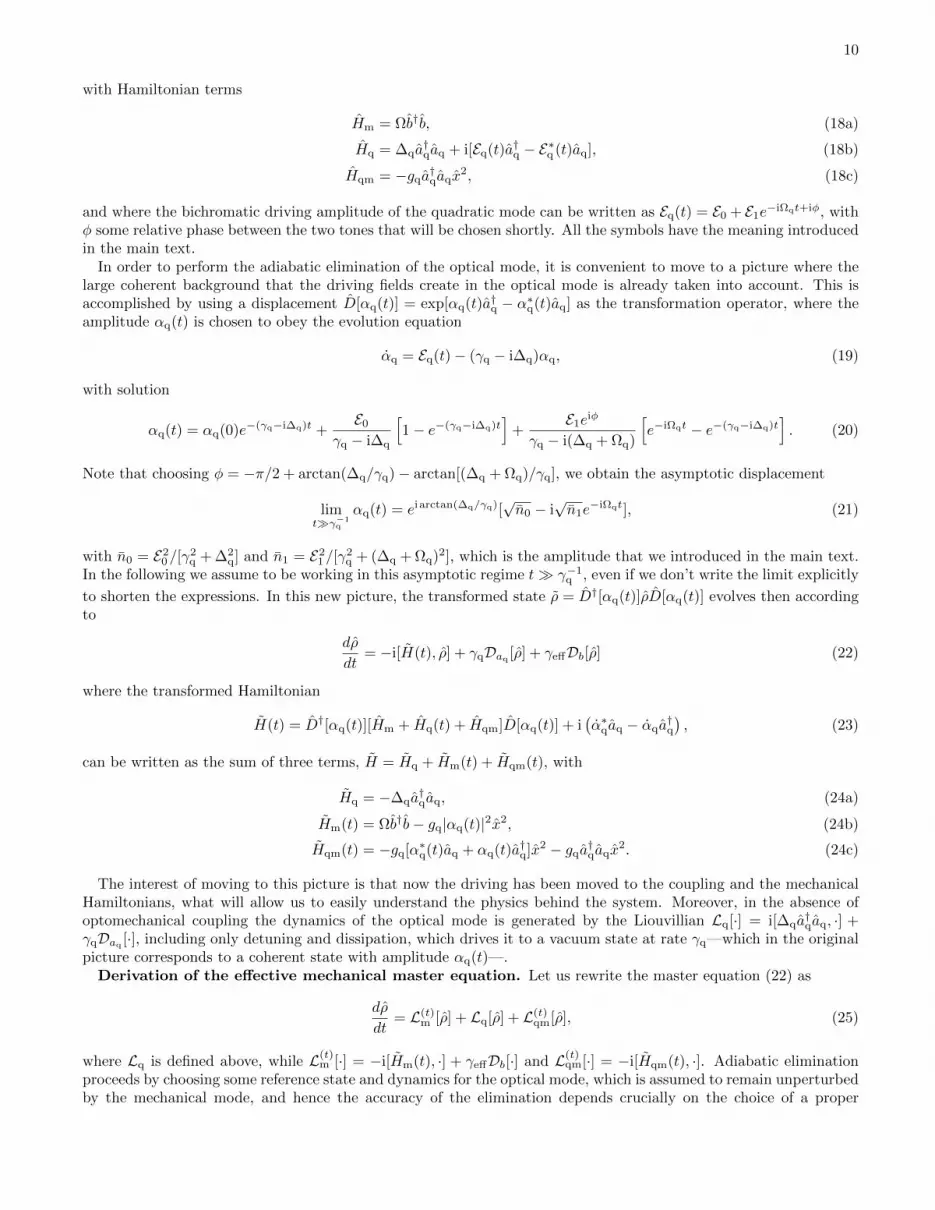
Moving to a simpler picture. Our starting point is the master equation of the optomechanical system as weintroduced it in the main text:

dρ

dt= −i[Hm + Hq(t) + Hqm, ρ] + γqDaq [ρ] + γeffDb[ρ], (17)

10

with Hamiltonian terms

Hm = Ωb†b, (18a)

Hq = ∆qa†qaq + i[Eq(t)a†q − E∗q (t)aq], (18b)

Hqm = −gqa†qaqx

2, (18c)

and where the bichromatic driving amplitude of the quadratic mode can be written as Eq(t) = E0 + E1e−iΩqt+iφ, withφ some relative phase between the two tones that will be chosen shortly. All the symbols have the meaning introducedin the main text.

In order to perform the adiabatic elimination of the optical mode, it is convenient to move to a picture where thelarge coherent background that the driving fields create in the optical mode is already taken into account. This isaccomplished by using a displacement D[αq(t)] = exp[αq(t)a†q − α∗q(t)aq] as the transformation operator, where theamplitude αq(t) is chosen to obey the evolution equation

αq = Eq(t)− (γq − i∆q)αq, (19)

with solution

αq(t) = αq(0)e−(γq−i∆q)t +E0

γq − i∆q

[1− e−(γq−i∆q)t

]+

E1eiφ

γq − i(∆q + Ωq)

[e−iΩqt − e−(γq−i∆q)t

]. (20)

Note that choosing φ = −π/2 + arctan(∆q/γq)− arctan[(∆q + Ωq)/γq], we obtain the asymptotic displacement

limtγ−1

q

αq(t) = eiarctan(∆q/γq)[√n0 − i

√n1e−iΩqt], (21)

with n0 = E20/[γ

2q + ∆2

q] and n1 = E21/[γ

2q + (∆q + Ωq)2], which is the amplitude that we introduced in the main text.

In the following we assume to be working in this asymptotic regime t γ−1q , even if we don’t write the limit explicitly

to shorten the expressions. In this new picture, the transformed state ρ = D†[αq(t)]ρD[αq(t)] evolves then accordingto

dρ

dt= −i[H(t), ρ] + γqDaq [ρ] + γeffDb[ρ] (22)

where the transformed Hamiltonian

H(t) = D†[αq(t)][Hm + Hq(t) + Hqm]D[αq(t)] + i(α∗qaq − αqa

†q

), (23)

can be written as the sum of three terms, H = Hq + Hm(t) + Hqm(t), with

Hq = −∆qa†qaq, (24a)

Hm(t) = Ωb†b− gq|αq(t)|2x2, (24b)

Hqm(t) = −gq[α∗q(t)aq + αq(t)a†q]x2 − gqa†qaqx

2. (24c)

The interest of moving to this picture is that now the driving has been moved to the coupling and the mechanicalHamiltonians, what will allow us to easily understand the physics behind the system. Moreover, in the absence ofoptomechanical coupling the dynamics of the optical mode is generated by the Liouvillian Lq[·] = i[∆qa

†qaq, ·] +

γqDaq [·], including only detuning and dissipation, which drives it to a vacuum state at rate γq—which in the originalpicture corresponds to a coherent state with amplitude αq(t)—.

Derivation of the effective mechanical master equation. Let us rewrite the master equation (22) as

dρ

dt= L(t)

m [ρ] + Lq[ρ] + L(t)qm[ρ], (25)

where Lq is defined above, while L(t)m [·] = −i[Hm(t), ·] + γeffDb[·] and L(t)

qm[·] = −i[Hqm(t), ·]. Adiabatic eliminationproceeds by choosing some reference state and dynamics for the optical mode, which is assumed to remain unperturbedby the mechanical mode, and hence the accuracy of the elimination depends crucially on the choice of a proper

11

reference. For our purposes, it is enough to take the dynamics generated by Lq as the optical reference, and hence itssteady state ρq = |0〉q〈0| (vacuum) as the reference state. Let us then define the projector superoperator

P[·] = ρq ⊗ trq·, (26)

and its complement Q = 1 − P. These superoperators satisfy the useful relations PL(t)m [·] = L(t)

m P[·] (obvious since

L(t)m acts on the mechanics only) and PLq[·] = 0 = LqP[·] (where the second equality is again obvious, while the first

one comes from Lq being traceless by conservation of probability).The next step consists on projecting the master equation onto the corresponding subspaces defined by these super-

operators. Defining the projected components of the density operator u(t) = P[ρ(t)] and w(t) = Q[ρ(t)], and usingthe properties of the projectors, it is straightforward to get the coupled linear system

du

dt=(L(t)

m + PL(t)qm

)[u] + PL(t)

qm[w], (27a)

dw

dt=(L(t)

m + Lq + PL(t)qm

)[w] +QL(t)

qm[u]. (27b)

The second equation can be formally integrated, leading to

w(t) =

∫ t

0

dt′Te∫ tt′ dt

′′(L(t′′)

m +Lq+PL(t′′)qm

)QL(t′)

qm [u(t′)], (28)

where T is the time-ordering superoperator, and we have not written the term which depends on the initial value w(0)since in this concrete dissipative scenario any information related to it has to be completely washed out asymptotically.Next, we introduce this formal solution in the first equation, and perform a Born approximation in which we neglectterms beyond quadratic order in the interaction Lqm, what allows us to write

du

dt= L(t)

m [u] + PL(t)qm[u] +

∫ t

0

dτPL(t)qmU (t−τ,t)

m eLqτQL(t−τ)qm [u(t− τ)], (29)

where in addition we have made the variable change t′ = t− τ in the integral, used the fact that Lm and Lq commute,and defined the mechanical time evolution superoperator

U (t−τ,t)m = T

e∫ tt−τ dt

′L(t′)m

. (30)

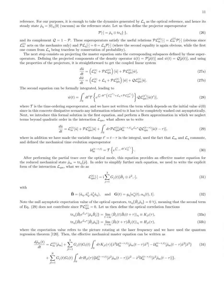
After performing the partial trace over the optical mode, this equation provides an effective master equation forthe reduced mechanical state ρm = trqρ. In order to simplify further such equation, we need to write the explicitform of the interaction Lqm, what we do as

L(t)qm[·] = i

3∑j=1

Gj(t)[Bj ⊗ x2, ·], (31)

with

B = (aq, a†q, a†qaq), and G(t) = gq[α∗q(t), αq(t), 1]. (32)

Note the null asymptotic expectation value of the optical operators, trqBj ρq = 0 ∀j, meaning that the second term

of Eq. (29) does not contribute since PL(t)qm = 0. Let us then define the optical correlation functions

trqBleLqτ [ρqBj ] = limt→∞〈Bj(t)Bl(t+ τ)〉q ≡ Kjl(τ), (33a)

trqBleLqτ [Bj ρq] = limt→∞〈Bl(t+ τ)Bj(t)〉q ≡ Hjl(τ), (33b)

where the expectation value refers to the picture rotating at the laser frequency and we have used the quantumregression theorem [120]. Then, the effective mechanical master equation can be written as

dρm(t)

dt= L(t)

m [ρm] +

3∑jl=1

Gj(t)Gl(t)

∫ t

0

dτKjl(τ)x2U (t−τ,t)m [ρm(t− τ)x2]− U (t−τ,t)

m [ρm(t− τ)x2]x2 (34)

+

N∑jl=1

Gj(t)Gl(t)

∫ t

0

dτHjl(τ)U (t−τ,t)m [x2ρm(t− τ)]x2 − x2U (t−τ,t)

m [x2ρm(t− τ)].

12

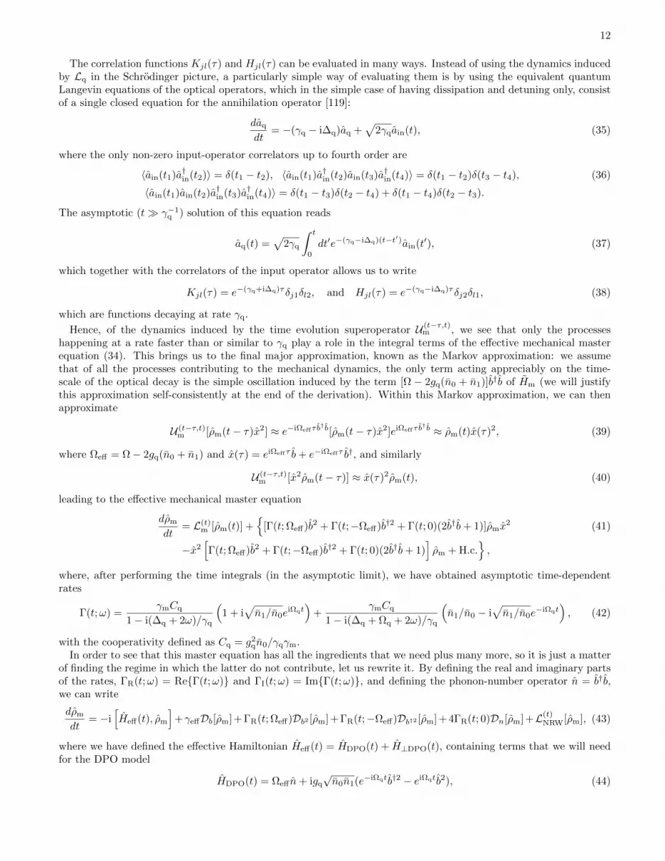
The correlation functions Kjl(τ) and Hjl(τ) can be evaluated in many ways. Instead of using the dynamics inducedby Lq in the Schrodinger picture, a particularly simple way of evaluating them is by using the equivalent quantumLangevin equations of the optical operators, which in the simple case of having dissipation and detuning only, consistof a single closed equation for the annihilation operator [119]:

daq

dt= −(γq − i∆q)aq +

√2γqain(t), (35)

where the only non-zero input-operator correlators up to fourth order are

〈ain(t1)a†in(t2)〉 = δ(t1 − t2), 〈ain(t1)a†in(t2)ain(t3)a†in(t4)〉 = δ(t1 − t2)δ(t3 − t4), (36)

〈ain(t1)ain(t2)a†in(t3)a†in(t4)〉 = δ(t1 − t3)δ(t2 − t4) + δ(t1 − t4)δ(t2 − t3).

The asymptotic (t γ−1q ) solution of this equation reads

aq(t) =√

2γq

∫ t

0

dt′e−(γq−i∆q)(t−t′)ain(t′), (37)

which together with the correlators of the input operator allows us to write

Kjl(τ) = e−(γq+i∆q)τδj1δl2, and Hjl(τ) = e−(γq−i∆q)τδj2δl1, (38)

which are functions decaying at rate γq.

Hence, of the dynamics induced by the time evolution superoperator U (t−τ,t)m , we see that only the processes

happening at a rate faster than or similar to γq play a role in the integral terms of the effective mechanical masterequation (34). This brings us to the final major approximation, known as the Markov approximation: we assumethat of all the processes contributing to the mechanical dynamics, the only term acting appreciably on the time-scale of the optical decay is the simple oscillation induced by the term [Ω − 2gq(n0 + n1)]b†b of Hm (we will justifythis approximation self-consistently at the end of the derivation). Within this Markov approximation, we can thenapproximate

U (t−τ,t)m [ρm(t− τ)x2] ≈ e−iΩeffτb

†b[ρm(t− τ)x2]eiΩeffτb†b ≈ ρm(t)x(τ)2, (39)

where Ωeff = Ω− 2gq(n0 + n1) and x(τ) = eiΩeffτ b+ e−iΩeffτ b†, and similarly

U (t−τ,t)m [x2ρm(t− τ)] ≈ x(τ)2ρm(t), (40)

leading to the effective mechanical master equation

dρm

dt= L(t)

m [ρm(t)] +

[Γ(t; Ωeff)b2 + Γ(t;−Ωeff)b†2 + Γ(t; 0)(2b†b+ 1)]ρmx2 (41)

−x2[Γ(t; Ωeff)b2 + Γ(t;−Ωeff)b†2 + Γ(t; 0)(2b†b+ 1)

]ρm + H.c.

,

where, after performing the time integrals (in the asymptotic limit), we have obtained asymptotic time-dependentrates

Γ(t;ω) =γmCq

1− i(∆q + 2ω)/γq

(1 + i

√n1/n0e

iΩqt)

+γmCq

1− i(∆q + Ωq + 2ω)/γq

(n1/n0 − i

√n1/n0e

−iΩqt), (42)

with the cooperativity defined as Cq = g2qn0/γqγm.

In order to see that this master equation has all the ingredients that we need plus many more, so it is just a matterof finding the regime in which the latter do not contribute, let us rewrite it. By defining the real and imaginary partsof the rates, ΓR(t;ω) = ReΓ(t;ω) and ΓI(t;ω) = ImΓ(t;ω), and defining the phonon-number operator n = b†b,we can write

dρm

dt= −i

[Heff(t), ρm

]+γeffDb[ρm] + ΓR(t; Ωeff)Db2 [ρm] + ΓR(t;−Ωeff)Db†2 [ρm] + 4ΓR(t; 0)Dn[ρm] +L(t)

NRW[ρm], (43)

where we have defined the effective Hamiltonian Heff(t) = HDPO(t) + H⊥DPO(t), containing terms that we will needfor the DPO model

HDPO(t) = Ωeff n+ igq

√n0n1(e−iΩqtb†2 − eiΩqtb2), (44)

13

plus some that we don’t want to contribute

H⊥DPO(t) = [4gq

√n0n1 sin(Ωqt)− ΓI(t; Ωeff) + 3ΓI(t;−Ωeff) + 4ΓI(t; 0)]n (45)

+ [ΓI(t; Ωeff) + ΓI(t;−Ωeff) + 4ΓI(t; 0)]n2 − [gq(n0 + n1 + i√n0n1e

iΩqt)b†2 + H.c.],

and we have collected into LNRW the terms which in the absence of the sideband are expected not to contribute withinthe rotating wave approximation, which read

L(t)NRW[ρm] = [Γ(t; Ωeff) + Γ∗(t;−Ωeff)]b2ρmb

2 − Γ(t; Ωeff)b4ρm − Γ∗(t;−Ωeff)ρmb4 (46)

+ [Γ(t; Ωeff) + Γ∗(t; 0)]b2ρm(2n+ 1)− Γ(t; Ωeff)(2n+ 1)b2ρm − Γ∗(t; 0)ρm(2n+ 1)b2

+ [Γ(t; 0) + Γ∗(t;−Ωeff)](2n+ 1)ρmb2 − Γ(t; 0)b2(2n+ 1)ρm − Γ∗(t;−Ωeff)ρmb

2(2n+ 1) + H.c..

Degenerate parametric oscillation regime. Let’s now discuss the conditions under which the effective me-chanical master equation above will correspond to the master equation of the DPO, Eq. (8).

Looking at the term HDPO(t) of the effective Hamiltonian, we see that the sideband Ωq should be chosen to matchtwice the effective mechanical frequency, that is, 2Ωeff .

On the other hand, we would like the effective two-phonon cooling Db2 to dominate over any other irreversibleprocess, in particular over the two-phonon heating Db†2 and dephasing Dn, and to do so with a time-independentrate. Looking at (42), the latter can be naturally accomplished by driving the fundamental tone much stronger thanthe sideband, that is, n0 n1. The static part of the rates (42) then suggests that cooling will be enhanced bychoosing a detuning of the fundamental driving tone matching the red two-phonon sideband, ∆q = −2Ωeff ; indeed,this choice provides the following real, static part of the rates

Γcooling = γmCq, Γheating =γmCq

1 + 16Ω2eff/γ

2q

, and Γdephasing =γmCq

1 + 4Ω2eff/γ

2q

, (47)

showing in addition that we need to work in the resolved sideband regime 4Ω2eff γ2

q in order for heating anddephasing to be suppressed; in particular, we will define the parameter r = (1 + 4Ω2

eff/γ2q)−1 1, which allows us to

approximate the rates by

Γ(t; Ωeff) = γmCq

(1 + i

√rn1/n0 + i

√n1/n0e

2iΩeff t +√r(n1/n0)e−2iΩeff t

), (48a)

Γ(t;−Ωeff) = −i√rγmCq

(1 + i

√n1/n0e

2iΩeff t − 2i√n1/n0e

−2iΩeff t)/2, (48b)

Γ(t; 0) = γmCq

(n1/n0 − i

√r +

√r(n1/n0)e2iΩeff t − i

√n1/n0e

−2iΩeff t), (48c)

expressions that together with working in the weak sideband regime, n1/n0 1, suggest that the only relevant rateis the real static part of Γ(t; Ωeff) which provides the two-phonon cooling rate as desired.

The next constrain on the parameters comes from the fact that there are many counter-rotating terms that we

want not to contribute within the rotating-wave approximation. Among these, inspection of L(t)NRW and H⊥DPO shows

that the largest of such rates are γmCq and gq(n0 + n1) ≈ gqn0, but note that gqn0/γmCq = γq/gq which is typicallymuch larger than 1 (optomechanical systems work far from the single-photon strong coupling regime, specially whenreferring to the quadratic coupling), and hence gqn0 is the largest of these two rates. Thus, the rotating wave-approximation requires gqn0 Ωeff . Provided that this approximation holds, we can neglect all the counter-rotating

terms in H⊥DPO and L(t)NRW, approximating them by

H⊥DPO ≈ −√rγmCq(11 + 9n)n/2, (49)

and

L(t)NRW[ρm] =

√n1/n0γmCqe

2iΩeff t[ib2ρm(2n+ 1)− i(2n+ 1)b2ρm +√rρm(2n+ 1)b2 (50)

−√rb2(2n+ 1)ρm +√rρmb

2(2n+ 1)] + H.c..

This expression clearly shows that L(t)NRW is negligible when compared with the two-phonon cooling term γmCqDb2 .

On the other hand, H⊥DPO provides a negligible effective mechanical frequency shift, but also a Kerr term which isexpected to be negligible only as long as 〈n〉 Ωeff/4.5

√rγmCq, which puts a bound on the number of phonons.

14

Nevertheless, for the parameters corresponding to a realistic implementation used in the main text, we find this boundto be ∼ 1013, while the classical limit of the DPO tells us that the phonon number expected at σ = 2.5 is on the orderof 1010, three orders of magnitude below the limit in which the Kerr term can start playing a role.

Provided that all these considerations are taken into account, we then expect the effective mechanical masterequation to be very well approximated by

dρm

dt≈ −i

[Heff(t), ρm

]+ γeffDb[ρm] + γmCqDb2 [ρm], (51)

with effective Hamiltonian

Heff(t) ≈ Ωeff n+ igq

√n0n1(e−2iΩeff tb†2 − e2iΩeff tb2), (52)

which is exactly the DPO model, Eq. (8).Note that there is a final constrain on the parameters coming from the Markov approximation that we performed

in the adiabatic elimination: since we assumed that within the decay of the optical correlators at rate γq the onlyrelevant mechanical process is the simple oscillation at frequency Ωeff , we need the rates γeff , γmCq, and gq

√n0n1,

to be smaller than γq. For the parameters considered in the main text, γeff is the largest rate of the three (for an n1

corresponding to σ = 2.5 in the DPO model or smaller), and it satisfies γeff/γq ≈ 6 × 10−3, so we are safely withinthe Markov regime.

ASYMPTOTIC STATE OF THE FULL MODEL

Let us in this final section of the supplemental material explain how we have found the asymptotic state of theoptomechanical model numerically. As with the stationary state of the DPO model, we have performed simulationsof the full master equation (17), as well as simulations in the classical limit.

In the first case, our starting point has been the optomechanical master equation in the displaced picture, Eq.(22). For numerical purposes, it is important to work in this displaced picture because the state of the optical modeshould stay close to vacuum, while in the original picture it is a highly populated coherent state which does notallow for a reasonable truncation of the optical Fock space. As before, we set the truncation of the mechanical andoptical Fock bases in such a way that the mean phonon number finds convergence up to the third significant digit,what typically does not require more than one or two photons in this displaced picture. The simulation proceedsagain as explained in detail in [91], that is, by moving to superspace where the master equation (22) is turned intoa linear system d~ρ(t)/dt = L(t)~ρ(t). Note that now the linear problem is manifestly time-dependent, and therefore,there will be no steady state. In particular, L(t) is 2π/Ωq-periodic, and this periodicity is reflected into a time-dependent asymptotic state ρ(t) = limt→∞ ρ(t), which we find by solving the linear system numerically startingfrom different initial conditions ~ρ(0), that is, different initial states ρ(0). In all the simulations we have checkedthat the asymptotic state is independent of the chosen initial state (e.g., vacuum or the steady state of the DPOfor the mechanics). As explained in the text, the observable we have focused on is the asymptotic phonon number

limt→∞〈b†b(t)〉 = trb†bρ(t), whose time evolution can be approximated by a function of the type n + δn sin(Ωqt),with δn n.

The superspace simulation of the master equation becomes quite heavy as the mechanical state gets populated,what has prevented us from performing simulations for values of the sideband power where the system is expected tobe above the DPO phase transition. Hence, in order to prove that the optomechanical model leads to the expectedphase transition, we have performed simulations of the optomechanical system in the classical limit. Similarly to whatwe did for the DPO model in the first section, this limit is found by assuming that both the optical and mechanicalmodes are in a coherent state at all times. Let us show the procedure explicitly for this case too. Our starting point isthe original optomechanical master equation (17), but replacing the mechanical dissipator Db[·] by [x, p, ·]/2i, where

p = i(b†− b) is the mechanical momentum quadrature. For high-Q mechanical oscillators which admit a weak-couplingdescription of their interaction with the environment, this dissipator leads to the same physics as the previous one[119], but provides better-looking classical equations. With this change, the evolution of the expectation value of anysystem operator A reads

d〈A〉dt

= tr

Adρ

dt

= −i〈[A, Hm + Hq(t) + Hqm]〉+ γq(〈[a†q, A]aq〉+ 〈a†q[A, aq]〉) +

γeff

2i〈[A, x], p〉, (53)

where just as with the DPO model, we are defining the expectation value with respect to the state in the picturerotating at the laser frequency, that is, 〈·〉 = tr· ρ, with ρ the state in the rotating frame. Applied to aq, x, and

15

p, and denoting by α(t) and β(t) the amplitudes of the optical and mechanical coherent states, we find the classicalevolution equations

x = Ωp, (54a)

p = −2γeffp− (Ω− 4gq|α|2)x, (54b)

α = Eq(t)− (γq − i∆q − igqx2)α, (54c)

with the classical mechanical position and momentum defined as x = 2Reβ and p = 2Imβ, respectively. Thisnonlinear system can be efficiently simulated numerically for (practically) any parameter set, and the phonon number

that it predicts can be evaluated as limt→∞〈b†b(t)〉 = limt→∞[x2(t) + p2(t)]/4, which again can be approximated byn+ δn sin(Ωqt), with (typically) δn n.